ibf - updates - 2007 (q1 & q2 v1.0)
DESCRIPTION
The following 55+ pages represent a summary of relevant information from the first and second quarter of 2007.TRANSCRIPT

Copyright © 2007 by Institute of Business and Finance. All rights reserved. v1.0
INSTITUTE OF BUSINESS & FINANCE
QUARTERLY
UPDATES
2007 Q1 & Q2


Quarterly Updates
Table of Contents
MUTUAL FUNDS
DISTURBING RETURN FIGURES 1.1
YEAR-END WINDOW DRESSING 1.1
PICKING THE NEXT TOP PERFORMERS 1.2
A RANDOM WALK 1.2
LARGEST FUND COMPANIES 1.4
CORRELATIONS TO THE S&P 500 REVISITED 1.5
STYLE BOXES 1.6
FOCUSED FUNDS AND RISK 1.7
LIFECYCLE FUNDS 1.8
TARGET-DATE FUNDS EXPAND 1.8
MORE AGGRESSIVE LIFE CYCLE FUNDS 1.9
LONG-SHORT FUNDS 1.10
DIVERSIFICATION BENEFITS 1.10
FREQUENCY OF PORTFOLIO REBALANCING 1.12
VALUE LINE HYPE 1.12
ODDS OF BEATING AN INDEX 1.13
MIXED PERFORMANCE RANKINGS 1.15
ACTIVE VS. PASSIVE MANAGEMENT 1.16
SIDE-BY-SIDE MANAGEMENT 1.17
MANAGER-INVESTED MUTUAL FUNDS 1.19
B SHARES REVIEWED BY SEC 1.25
SHAREHOLDER PROXY VOTING 1.26
SECURITIES LENDING PRACTICES 1.27
FUND DIRECTOR PAY 1.28
DIRECTORS AND 12B-1 FEES 1.28
STOCKS AND MUTUAL FUNDS 1.29

ETFS
ETF UPDATE 2.1
THE LARGEST ETFS 2.4
ETFS WITH LOW EXPENSE RATIOS 2.5
ETF PRICE DISPARITIES 2.6
SECTOR VOLATILITY 2.7
BUYING AND SELLING ETFS 2.8
UITS AND CLOSED-END FUNDS
UIT AND NEW FUND CRITICISM 3.1
CLOSED-END FUND ASSET INCREASE 3.1
CLOSED-END COVERED CALL FUNDS 3.2
REITS
REIT UPDATE 4.1
INTERNATIONAL REITS 4.2
STOCKS
DOW MILESTONES 5.1
DOW DROPS 5.2
S&P 500 AND DJIA RETURNS 5.3
SMALL CAP STOCKS 5.4
QUALIFYING DIVIDENDS 5.4
BUFFET WARNING 5.4
DIVIDEND-PAYING BONUS 5.5
VALUE PLAY 5.5
VALUE VS. GROWTH STOCKS
ROLLING PERIODS: GROWTH VS. VALUE 6.1
REVISITING GROWTH AND VALUE 6.2
SMALL CAP VALUE 6.7
GROWTH VS. VALUE 6.8
2006 INDEX RETURNS 6.9
BONDS
CUSHION AGAINST STOCK DECLINES 7.1
STOCKS VS. BONDS 7.1
2006 HIGH-YIELD BOND FACTS 7.2
BOND MARKETS, INDEXES, AND FUNDS 7.3
GLOBAL INVESTING
WORLD’S FINANCIAL ASSETS 8.1
EMERGING MARKET DEBT 8.2
2006 GLOBAL INDEX RETURNS 8.2
REDUCED GLOBAL CORRELATION 8.3
EAFE COMPOSITION 8.4
GLOBAL SMALL CAP BENEFITS 8.6
DOMESTIC GLOBAL DIVERSIFICATION 8.7
COVERED CALL WRITING
SPDRS AND COVERED CALL WRITING 9.1
EQUITY-INDEXED ANNUITIES
EQUITY-INDEXED ANNUITIES (EIAS) 10.1
FINANCIAL PLANNING
OPTIMAL REBALANCING 11.1
PREDICTED MARKET MELTDOWN 11.4
DISTRIBUTION OF RETURNS 11.5
INVESTING IN A HOUSE 11.6
AMERICA THE BANKRUPT? 11.7
CPI SPENDING CATEGORIES 11.7
GOLD VS. HERSHEY BARS 11.9
HEDGE FUND DISASTERS 11.10
HEDGE FUND WARNING 11.11
CALCULATING A LUMP SUM 11.11
ENDING UP WITH $1,000,000 11.12
GOALS AND RISK TOLERANCE TEST 11.12
RETIREMENT PLANNING
RECONSIDERING THE ROTH 401(K) 12.1
HEALTH SAVINGS PLANS 12.2
529 PLANS 12.3
RETIREMENT PLAN INCREASES FOR 2007 12.3
RETIREMENT REALITY 12.7
BENEFITS OF PATIENCE 12.8
COSTS OF 401(K) PLANS 12.9
RETIREMENT STATISTICS 12.10
MAXIMUM SOCIAL SECURITY BENEFIT 12.10
PEOPLE WORKING LONGER 12.11
INFLATION MEASUREMENTS 12.11
LONG-TERM CARE PARTNERSHIP 12.15
DISCLOSURE PROTECTION FOR ORGAN DONORS 12.17
FULLY FUNDED PENSION PLANS 12.18
NEW MEDICAID RULES 12.18
TAXES
2007 TAX BREAKS 13.1
TAX DOCUMENTS 13.2
FREE TAX PREPARATION AND FILING 13.3
TAX FACTS 13.3
APPEAL TO CHILDREN 13.5
FEDERAL RESERVE COMIC BOOKS 13.6
YOUNG INVESTORS 13.6

QUARTERLY
UPDATES
MUTUAL FUNDS


MUTUAL FUNDS 1.1
QUARTERLY UPDATES
IBF | GRADUATE SERIES
1.DISTURBING RETURN FIGURES
According to DALBAR, the average equity mutual fund investor
experienced annualized returns of just 3.9% over the 20-year period
ending December 31st, 2005. During this same period, inflation
averaged 3% a year, while a buy-and-hold investment in the S&P
500 returned 11.9% a year.
YEAR-END WINDOW DRESSING
For roughly the last week or two of the year, many mutual and hedge
fund managers sell off poorly performing securities and replace them
with the quarter’s best performers. Over the past 16 years, the S&P
500’s top-performing stocks of the first 11 weeks or so of the fourth
quarter have outperformed the overall index by an average of 2.6%
in the final week; this strategy has worked every year.
The Thomson Financial study suggests the efficiency comes from
buying all of the top 50 performers and then selling them just before
the first trading day of the next year. Another strategy worth
considering is to buy stocks that are among the market’s worst 10%
performers. Over the past 16 years, these stocks have beaten the
S&P 500 by 1.8% in the first week of the new year (vs. 0.7% for the
top-performing stocks).
1.2 MUTUAL FUNDS
QUARTERLY UPDATES
IBF | GRADUATE SERIES
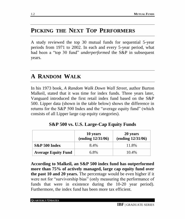
PICKING THE NEXT TOP PERFORMERS
A study reviewed the top 30 mutual funds for sequential 5-year
periods from 1971 to 2002. In each and every 5-year period, what
had been a “top 30 fund” underperformed the S&P in subsequent
years.
A RANDOM WALK
In his 1973 book, A Random Walk Down Wall Street, author Burton
Malkeil, stated that it was time for index funds. Three years later,
Vanguard introduced the first retail index fund based on the S&P
500. Lipper data (shown in the table below) shows the difference in
returns for the S&P 500 Index and the “average equity fund” (which
consists of all Lipper large cap equity categories).
S&P 500 vs. U.S. Large-Cap Equity Funds
10 years
(ending 12/31/06)
20 years
(ending 12/31/06)
S&P 500 Index 8.4% 11.8%
Average Equity Fund 6.8% 10.4%
According to Malkeil, an S&P 500 index fund has outperformed
more than 75% of actively managed, large cap equity fund over
the past 10 and 20 years. The percentage would be even higher if it
were not for “survivorship bias” (only measuring the performance of
funds that were in existence during the 10-20 year period).
Furthermore, the index fund has been more tax efficient.

MUTUAL FUNDS 1.3
QUARTERLY UPDATES
IBF | GRADUATE SERIES
In 1970 there were 355 equity funds, only 117 were still in
existence at the end of 2006. Of the surviving 117 funds, 57
underperformed the S&P 500, 38 had equivalent returns, and 22
outperformed the index. Looking at the funds that either closely
matched or outperformed the S&P 500, 27 outperformed the index
by 0-1%, 16 by 1%, two by 2%, one by 3%, and one by 4%.
Malkeil acknowledges that the Fundamental Index has done well
during the early 2000s, but that such performance has been due to
the fundamental index’s bias toward value and small cap. The author
further points out that there have certainly been times when “the
market makes mistakes—it goes crazy sometimes.” As an example,
at the height of the market bubble in 2000, Cisco represented 4% of
the S&P 500, yet it represented just 0.02% of the economy. In 1999,
Amazon had a market value over $30 billion, even though it had yet
to ever make a profit. In fact, its losses for 1999 were over $600
million. At its height, technology stocks represented a third of
the S&P 500 (according to TheStreet.com, telecom and technology
combined represented 45% of the S&P 500 as of March 2000).
According to Malkeil, “My argument for indexing was based on my
belief that our equity markets are remarkably efficient. When
information arises about the stock market or individual stocks, that
information gets reflected without delay—switching from stock to
stock in an attempt to provide superior performance—is unlikely to
be effective, especially when you add in trading costs and taxes.”

1.4 MUTUAL FUNDS
QUARTERLY UPDATES
IBF | GRADUATE SERIES
LARGEST FUND COMPANIES
According to Lipper, the 30 largest mutual fund families manage
more than 75% of the industry’s assets; the top 10 companies
control 47% and the biggest 60 oversee nearly 91% of all mutual
fund assets. The table below shows the top 10 fund companies, as of
the end of the third quarter 2006 (note: “b” = billion and “t” =
trillion).
Largest Mutual Fund Companies [as of 9-30-2006]
Company
Open-
End
Closed-
End
Variable
Annuities
Total
%
Fidelity $1 t $0 $60 b $1.1 t 11%
Vanguard $1 t $0 $10 b $1.0 t 10%
American Funds $925 b $0 $85 b $1.0 t 10%
Franklin / Templeton $280 b $4.3 b $30 b $315 b 3%
BlackRock / Merrill $250 b $31 b $9 b $290 b 3%
Bank of America / Fleet $230 b $0.9 b $5.9 b $240 b 2%
Morgan Stanley $195 b $16 b $17 b $225 b 2%
Allianz / PIMCO $200 b $12 b $14 b $225 b 2%
JP Morgan / Chase $220 b $0.7 b $0.6 b $225 b 2%
Legg Mason / Citibank $200 b $8.7 b $9 b $220 b 2%
Industry Total $8.9 t $240 b $1.1 t $10.3 t 100%

MUTUAL FUNDS 1.5
QUARTERLY UPDATES
IBF | GRADUATE SERIES
CORRELATIONS TO THE S&P 500 REVISITED
A review of the past handful of years shows that the correlation
coefficient of a number of categories with the S&P 500 has
increased. As an example, from February 2000 to February 2006,
nine of the 10 different sectors in the S&P 500 (e.g., financials,
consumer cyclicals, energy, etc.) showed a correlation of at least
75% with the overall market. By contrast, in 2000, only two
sectors moved in such close step with the S&P 500. The table below
shows five-year correlations to the S&P for four different categories.
5-Year Correlations to the S&P 500
[Feb. 2000 and Feb. 2006]
Index 2000 correlation 2006 correlation
Hedge funds 35% 96%
MSCI EAFE 32% 96%
Russell 2000 62% 94%
Goldman Commodity -14% 33%
1.6 MUTUAL FUNDS
QUARTERLY UPDATES
IBF | GRADUATE SERIES
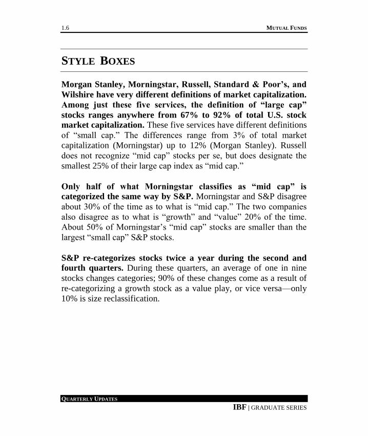
STYLE BOXES
Morgan Stanley, Morningstar, Russell, Standard & Poor’s, and
Wilshire have very different definitions of market capitalization.
Among just these five services, the definition of “large cap”
stocks ranges anywhere from 67% to 92% of total U.S. stock
market capitalization. These five services have different definitions
of “small cap.” The differences range from 3% of total market
capitalization (Morningstar) up to 12% (Morgan Stanley). Russell
does not recognize “mid cap” stocks per se, but does designate the
smallest 25% of their large cap index as “mid cap.”
Only half of what Morningstar classifies as “mid cap” is
categorized the same way by S&P. Morningstar and S&P disagree
about 30% of the time as to what is “mid cap.” The two companies
also disagree as to what is “growth” and “value” 20% of the time.
About 50% of Morningstar’s “mid cap” stocks are smaller than the
largest “small cap” S&P stocks.
S&P re-categorizes stocks twice a year during the second and
fourth quarters. During these quarters, an average of one in nine
stocks changes categories; 90% of these changes come as a result of
re-categorizing a growth stock as a value play, or vice versa—only
10% is size reclassification.
MUTUAL FUNDS 1.7
QUARTERLY UPDATES
IBF | GRADUATE SERIES
Critics of the nine equity style boxes point out that diversifying
across 13 widely-recognized asset classes, such as stocks, bonds,
money market, international, etc, is seven times more effective
than diversifying across the nine different stock categories. The
critics believe that potentially 74% of portfolio volatility can be
eliminated in this way (vs. only 11% amongst the different domestic
stock categories). In short, those who question stock style boxes
believe that U.S. stocks, regardless of size or being classified as
growth, value, or blend, are a single asset class, not six or nine.
FOCUSED FUNDS AND RISK
Focused funds that have low turnover tend to also have low
volatility. For example, mutual funds that were in the quartile with
the fewest stocks and in their category’s lowest-turnover quartile had
a lower standard deviation than the category average in over 75% of
rolling one-, three-, five-, and 10-year periods combined.
For the 2000, 2001, and 2002 calendar years, as a group,
concentrated funds performed better than their non-concentrated
peers. In 2001, funds in the most-concentrated quartile had
performance in the top 39% of their category’s average; the least
concentrated quartile averaged a 54% ranking.

1.8 MUTUAL FUNDS
QUARTERLY UPDATES
IBF | GRADUATE SERIES
LIFECYCLE FUNDS
Lifecycle fund assets increased by over 60% in 2006. Some financial
advisors are concerned that the equity exposure many of these funds
for those about to retire is too high (e.g., “2010 funds” have stock
exposures as high as 63% in the case of Charles Schwab and T.
Rowe Price). A University of Maryland finance professor
recommends using three lifecycle funds. For example, someone
retiring in 2015 could buy a 2015 fund to cover the first 10 years of
retirement, a 2025 fund to pay for the years from ages 75 to 85, and
a 2035 fund for the final years.
TARGET-DATE FUNDS EXPAND
As of early May 2007, there were 34 mutual fund companies that
offered one or more target-date funds. This $150 billion asset
category has increased in popularity partially because of the federal
pension bill, wherein target-date funds are frequently the default
option for 401(k) plan participants.
Besides growing in popularity, target-date funds have also expanded
the number of investment categories they invest in; emerging market
stocks, REITs, TIPS, private equity, commodities, leveraged loans,
and/or long-short funds are now being used by more and more of
these funds.

MUTUAL FUNDS 1.9
QUARTERLY UPDATES
IBF | GRADUATE SERIES
MORE AGGRESSIVE LIFE CYCLE FUNDS
A number of life cycle funds have increased their stock allocation
from 80% to 90% for younger investors. One life cycle fund for
those just retiring has 55% in common stocks and 10% in REITs; the
fund shifts to 25% in stocks, 10% in REITs, and 65% in fixed
income for those age 80. The fund company’s research found that a
1% higher annual return beginning at age 25 could fund “more than
10 additional years of retirement spending.”
When determining the appropriate asset mix for your older clients,
think of their Social Security payments as a fixed-rate annuity; this
means that most retirees will end up with a larger percentage
allocated to fixed income than they think. One way to calculate this
percentage is to add up all projected Social Security payments,
discounted by a present value percentage.
Other mutual fund life cycle studies reach four additional
conclusions: (1) investors tend to pick portfolios that are more
aggressive than their ages warrant; (2) when a couple retires, it
should be expected that at least one of them will reach their 90s; (3)
the biggest risk to retirees is outliving their assets; and (4) life cycle
funds are likely to grow at an even more robust rate after the passage
of the Pension Protection Act of 2006 (which encourages companies
to automatically enroll workers into qualified retirement plans—a
life cycle fund could be the default selection if the employee does
not pick another option).

1.10 MUTUAL FUNDS
QUARTERLY UPDATES
IBF | GRADUATE SERIES
LONG-SHORT FUNDS
Long-short funds ($14 billion in assets as of July 2006) are
sometimes confused with market neutral funds. Market neutral funds
balance their short and long positions, giving them a net market
exposure of zero; long-short funds either have a consistent long bias
or adjust their long-short mix tactically over time.
Long-short funds give smaller investors access to certain hedge
fund strategies and although they are less expensive than hedge
funds, costs can still be high. Some long-short funds have an
expense ratio as high as 4% (vs. 1.5% for the average domestic stock
fund). Over the past three years (ending 12/31/2006), long-short
funds averaged 7.5% annually.
DIVERSIFICATION BENEFITS
Many advisors have seen an “element chart” of investment
returns, asset category performance rankings over each of the
past several years. What few advisors have seen is such a chart
that includes not only growth and value plays, but REITs, mid
cap issues, and, most importantly, the ranking of a “diversified
portfolio” (defined as an equal weighting in each of the nine
asset classes ranked below).

MUTUAL FUNDS 1.11
QUARTERLY UPDATES
IBF | GRADUATE SERIES
Yearly Asset Category Rankings [1992-2006]
1992 1993 1994 1995 1996 1997 1998 1999 2000 2001 2002 2003 2004 2005 2006
SV
29%
FS 33%
FS 8%
LG 38%
RE 36%
LG 37%
LG 42%
SG 42%
RE 26%
RE 15%
IB 10%
SG 49%
RE 30%
FS 14%
RE 34%
HY
16%
SV
24%
LG
3%
LV
37%
LG
24%
MC
32%
FS
20%
LG
28%
SV
23%
SV
14%
RE
5%
SV
46%
SV
22%
MC
13%
FS
27%
RE 12%
LV 19%
RE 1%
SG 31%
LV 22%
SV 32%
MC 19%
FS 27%
MC 18%
IB 8%
HY -1%
FS 39%
FS 21%
RE 8%
SV 23%
MC
12%
RE
19% DP
0%
MC
31%
SV
21%
LV
30%
LV
14%
MC
15%
IG
12%
HY
5%
SV
-11%
RE
38%
MC
16% DP
7%
LV
21%
LV 11%
HY 17%
LV -1%
SV 26%
MC 19%
DP
21%
DP
9%
DP
13%
LC 6%
MC -1%
DP
-12%
MC 36%
DP
16%
LV 6%
DP
17%
DP
10%
DP
17%
HY
-1% DP
26%
DP
17%
RE
19%
IB
9%
LV
13% DP
2%
DP
-1%
MC
-15% DP
33%
LV
16%
SV
5%
SG
13%
SG 8%
MC 14%
SV -2%
HY 19%
HY 11%
SG 13%
HY 2%
HY 2%
HY -6%
SG -9%
FS -16%
LV 32%
SG 14%
SG 4%
HY 12%
IG
7%
SG
13%
SG
-2%
IG
18%
SG
11%
HY
13%
SG
1%
IG
-1%
FS
-14%
LV
-12%
LV
-21%
HY
29%
HY
11%
LG
3%
LG
11%
LG
5%
IG
10%
IG
-3%
RE
18%
FS
6%
IG
10%
SV
-6%
SV
-1%
LG
-22%
LG
-13%
LG
-24%
LG
-26%
LG
6%
HY
3%
MC
10%
FS
-12%
LG
-2%
MC
-4%
FS
12%
IG
4%
FS
2%
RE
-19%
RE
-6%
SG
-22%
FS
-21%
SG
-30%
IG
4%
IG
4%
IG
2%
IG
4%
SV = Russell 2000 Value Index MC = S&P MidCap 400 Index IG = Lehman Aggregate Bond Index
SG = Russell 2000 Growth Index FS = EAFE Index RE = FTSE NAREIT REIT Index
LG = S&P 500 / Barra Growth Index HY = Lehman High-Yield Index DP = equal parts of other 9 indexes
LV = S&P 500 / Barra Value Index
Observations
Large growth ranked at the top or bottom—never in the middle.
REITs ranked number one more than any other category.
Quality bonds ranked last more than any other category.
The diversified portfolio always landed in the middle.

1.12 MUTUAL FUNDS
QUARTERLY UPDATES
IBF | GRADUATE SERIES
FREQUENCY OF PORTFOLIO REBALANCING
According to the Financial Planning Association (FPA), the
optimal interval for rebalancing is 15-17 months, on average.
Research shows that if a portfolio is rebalanced more than about
once every 16 months, winners are sold off too quickly. An October
2006 study by the Pension Research Council at Wharton showed that
only 10% of 401(k) participants studied rebalanced their accounts on
either an active or a passive basis (e.g., using a lifecycle or target
retirement fund). The study, which looked at over one million 401(k)
participants, showed that passive rebalancing increased returns by
84 basis points annually, versus just 26 basis points for those
who rebalanced on their own.
VALUE LINE HYPE
The Value Line Web site states, “A stock portfolio with #1 Ranked
stocks for Timeliness from The Value Line Investment Survey,
beginning in 1965 and updated at the beginning of each year, would
have shown a gain of 19,715% through December 31st, 2004. This
gain would have beaten the S&P 500 by more than 15 to 1 for the
same time span.

MUTUAL FUNDS 1.13
QUARTERLY UPDATES
IBF | GRADUATE SERIES
ODDS OF BEATING AN INDEX
For the five-year period ending December 31st, 2006, only 15% of
large value managers beat their respective index; 90% of large
growth managers beat their index. One group of managers is not any
smarter or intuitive than the other. The disparity shows that most
funds are less “style-pure” than “style specific” (e.g., large value
funds hold stocks other than those classified as “large value,”
whereas a large value index would have virtually all, if not all, of its
holdings in “large value”). For example, the typical large cap
growth fund has the following composition.
Composition of the Average U.S. Large Cap Growth Fund
49% large growth 10% mid-cap growth < 1% small blend
27% large blend 4% mid-cap blend < 1% small growth
6% large value < 1% small value
If new benchmarks are calculated using the actual weightings, 35%
of large cap growth managers outperformed their “index” over the
past five years ending December 31st, 2006; 38% in the case of large
cap value managers. For the three-year period ending 12/31/2006,
24% of small growth funds beat their weighted benchmark versus
39% of large growth funds. Such results may cast some doubt on
whether or not the common assumption that small caps are a better
arena for active management.

1.14 MUTUAL FUNDS
QUARTERLY UPDATES
IBF | GRADUATE SERIES
Looking at just annual returns, the pattern remains consistent within
a fairly narrow range. In 1998, 44% of mutual funds in the nine style
box categories (e.g., large cap growth, large cap value, large cap
blend, mid-cap growth, etc.). In 1999, when technology stocks
soared, 50% of the funds beat their custom benchmark; the same
results occurred for 2000 and 2001 and actually increased to 57% in
2002 (probably due to the large cash holdings that year when the
market dropped). When the market rebounded in 2003, only 35% of
actively managed funds outperformed their custom benchmark. In
2004, the number rose to 42%, 47% in 2005, and then fell to 35% for
the 2006 calendar year.
Over 90% of domestic stock funds have geometric mean market
capitalizations below that of the S&P 500; thus, these funds could
outperform the S&P 500 when small and mid cap stocks are in favor,
and underperform when large blue chips do well.
Not only has independent research come up with a dramatically
lower return figure than Value Line’s claim, recent data would
appear to support the independent research. The flagship Value Line
mutual fund (VLIFX) uses the same criteria that guide The Value
Line Investment Survey (according to the fund’s prospectus). Yet,
the fund has only outperformed the S&P 500 twice over the past 10
years. The fund’s 10-year record as of May 30th, 2006 was 6%
annually, versus 9% for the S&P 500. Over the past 15 years, the
fund averaged 9.1% versus 10.9% for the S&P 500.

MUTUAL FUNDS 1.15
QUARTERLY UPDATES
IBF | GRADUATE SERIES
MIXED PERFORMANCE RANKINGS
A 2007 study by DeiMeo Schneider shows that roughly 90% of
mutual fund managers whose performance ranking in the top quartile
for 10 years ending December 31st, 2006 also had performance that
was below its category’s median for at least three or more of those
10 years. It turns out that just over 50% of pension managers
whose 10-year record was in the top quartile experienced below
median results for at least five consecutive years during the same
10 years.
The results become even more extreme within certain categories.
Over two-thirds of the top quartile foreign equity fund managers and
just under 75% of the top quartile medium-term bond fund managers
underperformed their category’s median returns for three years or
more during the 10-year period. There was at least a five-year
continuous stretch of underperformance for 72% of mid-cap blend,
71% of REIT, and 70% for emerging market equity managers whose
performance ranked in the top quartile for the same 10 years ending
December 31st, 2006.
Overall, the study showed that, on average, 22% of top-quartile
managers were in the bottom half of their peer groups during any
given three-year period. Based on these findings, it appears that at
any given time, close to a quarter of the top-performing pension
fund managers and mutual fund managers will experience a
three-year stretch of underperformance at any given quarterly
review.

1.16 MUTUAL FUNDS
QUARTERLY UPDATES
IBF | GRADUATE SERIES
ACTIVE VS. PASSIVE MANAGEMENT
Advocates of passive management (index funds) rarely talk about
accurate benchmark comparisons. For example, the average large
cap value fund has only about 40% of its assets in large cap value
stocks; the balance is in a variety of other stocks such as small and
mid cap growth as well as value.
Over the past five years ending March 31st, 2007, only 15% of the
large cap value stock funds outperformed their benchmark. Using
“custom” benchmarks (meaning an index that is comprised of
equities that a particular asset category’s management actually
invests in), 35-47% of the managers outperform their “actual” index.
The editor of a Vanguard newsletter uses active management for his
core portfolio. The editor suggests using actively-managed funds for
those you have “the greatest confidence in; use passive index funds
in those categories you cannot find a super-compelling active
management.”

MUTUAL FUNDS 1.17
QUARTERLY UPDATES
IBF | GRADUATE SERIES
SIDE-BY-SIDE MANAGEMENT
A number of mutual fund managers are serving two masters: the
fund(s) they oversee and one or more hedge funds. Mutual funds
sharing managers with hedge funds include Ameriprise, Nationwide,
Pioneer, and Vanguard. There are 125 individual portfolio
managers simultaneously running mutual funds and hedge
funds. Total mutual fund assets potentially affected by this possible
conflict of interest is $450 billion.
In 2003, the U.S. House of Representatives approved a measure,
later shelved, that would have barred someone from running a hedge
fund and mutual fund at the same time. Early in 2007, an SEC
official testifying in front of Congress said such a practice “presents
significant conflicts of interest that could lead the adviser to favor
the hedge fund over other clients.” Indeed, there are a number of
ways such favoritism could occur:
1. sell shares of a security in a hedge fund before a similar sale
in the mutual fund;
2. instead of assigning a trade to a specific fund at the time of
execution, a manager could “cherry pick” trades (e.g., trade in
the morning and assign it to the hedge fund or mutual fund
later in the day depending on its performance);
3. managers who have access to a limited number of hot IPOs
might favor the hedge fund over the mutual fund (since the
hedge fund has higher management fees plus a typical 20%
performance incentive fee); and
4. shorting stocks in a hedge fund while holding a long position
in a mutual fund could cause the stock’s price to drop.

1.18 MUTUAL FUNDS
QUARTERLY UPDATES
IBF | GRADUATE SERIES
The SEC does not dictate how managers should address these
potential conflicts of interest. Academic studies are divided on
whether or not mutual fund investors are well served or hurt by
multiple-role (side-by-side) management.
A study by William & Mary’s Mason School of Business and the
Wharton School looked at more than 450 mutual funds run by
companies who also managed hedge funds between 1994 and 2004.
The study found that in such instances, the mutual fund investors
underperformed their peer group by 1.2% a year. A Loyola
University Chicago, University of California, and University of
Illinois study reviewed 200 mutual funds run by side-by-side
managers (who also ran hedge funds) with a similar investment style
and found that the mutual funds outperformed their peers by 1.5%
annually from 1990 through 2005.
Starting in 2006, the SEC began to require funds to disclose
other types of accounts run by the manager and total assets
affected. Such information is found in the fund’s statement of
additional information (SAI). To find out what types of funds are
managed by a fund company, advisors and investors can search
www.adviser info.sec.gov.

MUTUAL FUNDS 1.19
QUARTERLY UPDATES
IBF | GRADUATE SERIES
MANAGER-INVESTED MUTUAL FUNDS
Mutual fund managers who own shares of the funds they oversee
outperform, on average, funds that are not partially owned by
management. A 2006 study done by three business schools looked at
the total returns of 1,300 stock and bond funds. The study looked at
managers who owned shares (43% of the 1,300 funds) versus funds
with no management ownership (57%).
Manager-owned funds had a mean return of 8.7% vs. 6.2% for
funds with no management ownership; the highest percentage of
management ownership was with U.S. stock funds and lowest
with foreign bond funds.
As of the beginning of 2007, of the 500 mutual funds most highly
recommended by Morningstar, more than 150 managers had each
invested more than $1 million in their funds. The most extreme
example of management ownership was Bill D’Alonzo who
oversees Brandywine (BRWIX) and Brandywine Blue (BLUEX); he
had 100% of his liquid net worth invested in these two funds. Other
examples include: Selected American (SLASX) and Selected Special
(SLSSX), two funds whose employees and those affiliated with the
fund collectively owned over $2 billion worth of shares; Longleaf
employees and directors owned over $500 million of their funds;
Chuck Royce had $50 million of his own money invested in Royce
Total Return (RYTRX) and Royce Premier (RYPRX).
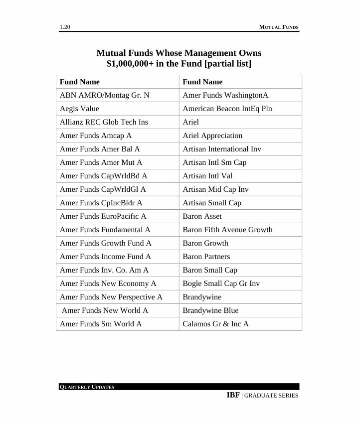
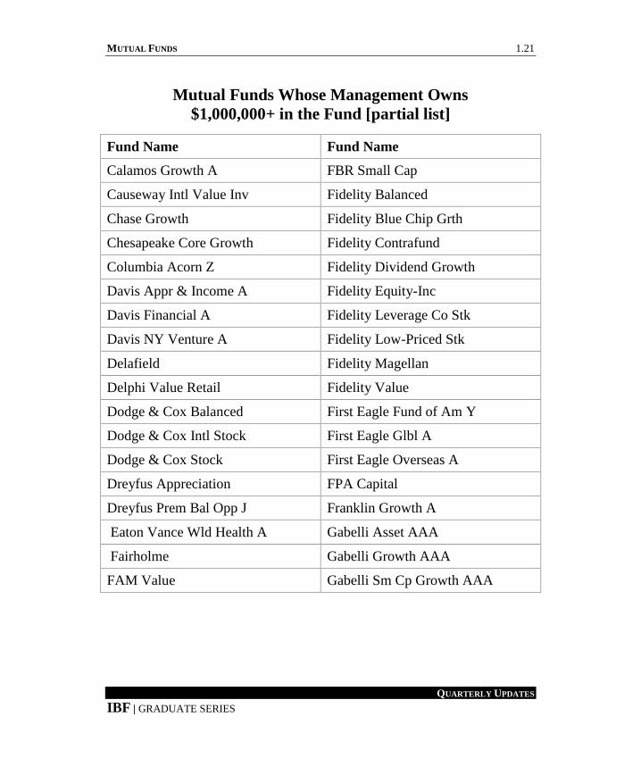
The extensive table below shows over 170 mutual funds whose
management owns over $1 million in their fund.
1.20 MUTUAL FUNDS
QUARTERLY UPDATES
IBF | GRADUATE SERIES
Mutual Funds Whose Management Owns
$1,000,000+ in the Fund [partial list]
Fund Name Fund Name
ABN AMRO/Montag Gr. N Amer Funds WashingtonA
Aegis Value American Beacon IntEq Pln
Allianz REC Glob Tech Ins Ariel
Amer Funds Amcap A Ariel Appreciation
Amer Funds Amer Bal A Artisan International Inv
Amer Funds Amer Mut A Artisan Intl Sm Cap
Amer Funds CapWrldBd A Artisan Intl Val
Amer Funds CapWrldGl A Artisan Mid Cap Inv
Amer Funds CpIncBldr A Artisan Small Cap
Amer Funds EuroPacific A Baron Asset
Amer Funds Fundamental A Baron Fifth Avenue Growth
Amer Funds Growth Fund A Baron Growth
Amer Funds Income Fund A Baron Partners
Amer Funds Inv. Co. Am A Baron Small Cap
Amer Funds New Economy A Bogle Small Cap Gr Inv
Amer Funds New Perspective A Brandywine
Amer Funds New World A Brandywine Blue
Amer Funds Sm World A Calamos Gr & Inc A
MUTUAL FUNDS 1.21
QUARTERLY UPDATES
IBF | GRADUATE SERIES
Mutual Funds Whose Management Owns
$1,000,000+ in the Fund [partial list]
Fund Name Fund Name
Calamos Growth A FBR Small Cap
Causeway Intl Value Inv Fidelity Balanced
Chase Growth Fidelity Blue Chip Grth
Chesapeake Core Growth Fidelity Contrafund
Columbia Acorn Z Fidelity Dividend Growth
Davis Appr & Income A Fidelity Equity-Inc
Davis Financial A Fidelity Leverage Co Stk
Davis NY Venture A Fidelity Low-Priced Stk
Delafield Fidelity Magellan
Delphi Value Retail Fidelity Value
Dodge & Cox Balanced First Eagle Fund of Am Y
Dodge & Cox Intl Stock First Eagle Glbl A
Dodge & Cox Stock First Eagle Overseas A
Dreyfus Appreciation FPA Capital
Dreyfus Prem Bal Opp J Franklin Growth A
Eaton Vance Wld Health A Gabelli Asset AAA
Fairholme Gabelli Growth AAA
FAM Value Gabelli Sm Cp Growth AAA

1.22 MUTUAL FUNDS
QUARTERLY UPDATES
IBF | GRADUATE SERIES
Mutual Funds Whose Management Owns
$1,000,000+ in the Fund [partial list]
Fund Name Fund Name
Gateway Fund Legg Mason Opp Prim
Harbor Capital App Instl Legg Mason Value Prim
Harbor Intl Instl LKCM Small Cap Equity Ins
Homestead Value Longleaf Partners
Hussman Strategic Growth Longleaf Partners Intl
ICAP Equity Longleaf Partners Sm-Cap
ICAP International Loomis Sayles Bond Ret
ICAP Select Equity Lord Abbett Affiliated A
Janus Marsico Focus
Janus Contrarian Fund Marsico Growth
Janus Enterprise Masters’ Select Equity
Janus Mid Cap Val Inv Matrix Advisors Value
Janus Orion Meridian Growth
Janus Overseas Meridian Value
Janus Sm Cap Val Instl Merrill Global Alloc A
Janus Twenty Muhlenkamp
Jensen J Mutual Shares A
Kalmar Gr Val Sm Cp Nicholas

MUTUAL FUNDS 1.23
QUARTERLY UPDATES
IBF | GRADUATE SERIES
Mutual Funds Whose Management Owns
$1,000,000+ in the Fund [partial list]
Fund Name Fund Name
Nicholas II I Royce Value Service
Northeast Investors RS Emerging Growth
Oak Value RS MidCap Opport
Oakmark Equity & Inc I Schneider Value
Oakmark Global I Selected American S
Oakmark I Sequoia
Oakmark International I Skyline Spec Equities
Oakmark Intl Small Cap I Sound Shore
Oakmark Select I T. Rowe Price Eq Inc
Osterweis Fund T. Rowe Price Gr Stk
Pioneer A T. Rowe Price Mid Gr
Pioneer High Yield A T. Rowe Price New Horiz
PRIMECAP Odyssey Agg Gr T. Rowe Price Sm Val
PRIMECAP Odyssey Growth Third Avenue Intl Value
Royce Opportunity Inv Third Avenue RealEst Val
Royce Premier Inv Third Avenue Sm-Cap Val
Royce Special Equity Inv Third Avenue Value
Royce Total Return Inv Thompson Plumb Growth

1.24 MUTUAL FUNDS
QUARTERLY UPDATES
IBF | GRADUATE SERIES
Mutual Funds Whose Management Owns
$1,000,000+ in the Fund [partial list]
Fund Name Fund Name
Thornburg Intl Value A Vanguard PRIMECAP Core
Thornburg Value A Vanguard Selected Value
Torray Vanguard Wellesley Inc
Turner Small Cap Growth Vanguard Wellington
Tweedy, Browne American Vanguard Windsor II
Tweedy, Browne Glob Val Wasatch Micro Cap
Van Kampen Comstock A Wasatch Small Cap Growth
Van Kampen Eq and Inc A Wasatch Ultra Growth
Van Kampen Growth & IncA Weitz Hickory
Vanguard Cap Opp Weitz Partners Value
Vanguard Capital Value Weitz Value
Vanguard Explorer Wesport R
Vanguard Health Care WF Adv Common Stk Z
Vanguard PRIMECAP WF Adv Opportunity Inv

MUTUAL FUNDS 1.25
QUARTERLY UPDATES
IBF | GRADUATE SERIES
B SHARES REVIEWED BY SEC
During 2006, the NASD imposed more than $40 million of fines on
brokerage firms for improperly selling B and C mutual fund shares.
During the early part of 2007, the SEC acknowledged that one of its
key arguments no longer exists; the agency had assumed A shares
were always better than B shares. The NASD commission now
believes that cost alone is not the only decision in making
investment recommendations.
Most of the lawsuits against brokerage firms were based on one of
three things: (1) failure to tell clients that A shares can be cheaper
than B shares, (2) fraud, and/or (3) suitability. In a 2007 case
dropped by the SEC, the agency acknowledged that even at the
$250,000 breakpoint, B shares may not be more expensive for the
client than A shares.
Because of regulatory concern, brokerage firms have generally
limited B share sales to $50,000 or less. Shares of B shares had
fallen to 3% of the market in 2006, down from 10% in 2001. One
broker, now retired, spent $400,000 in legal fees and lost $1.6
million in deferred compensation in 2001 when his broker-dealer
fired him over the sale of B shares. In late 2005, a NYSE arbitration
panel ordered the firm to pay all deferred compensation plus legal
fees.

1.26 MUTUAL FUNDS
QUARTERLY UPDATES
IBF | GRADUATE SERIES
SHAREHOLDER PROXY VOTING
During 2006, there were 1,400 filings by mutual funds asking
shareholders to vote on fund changes. The number of filings
represents about 20% of all mutual funds. During the first quarter of
2007, roughly 340 were seeking shareholder votes, according to
governance tracker the Corporate Library. The top issues voting
upon by shareholders have been issues dealing with directors and/or
trustees, investment restrictions and policies, and sub-advisor
agreements.
Fund companies want shareholders to vote as soon as possible for
such changes. If the necessary number of votes is not obtained, more
shareholder solicitation is required and this costs the fund, and
specifically its shareholders, more money. Among the most popular,
and worrisome proposals, are changes to investment limits,
loosening limits on borrowing and lending, requesting greater
flexibility in real estate and commodity investments, and taking
bigger positions in stocks or foreign holdings.
Despite investors’ concerns about proxy voting, shareholders rarely
show up at an announced meeting. For example, only 50 Dodge &
Cox investors showed up a few years ago to a meeting; only one
shareholder attended the $4.3 billion Alger Funds’ January meeting.

MUTUAL FUNDS 1.27
QUARTERLY UPDATES
IBF | GRADUATE SERIES
SECURITIES LENDING PRACTICES
Mutual funds and ETFs lend some of the securities in their portfolios
in exchange for interest payments and collateral, which provides
additional returns for fund investors (well under 1/10th of 1%).
Although this practice is not new, the explosive growth of hedge
funds engaged in short selling has greatly increased the demand for
borrowed securities.
When a hedge fund, or any investor, enters a short sale (betting a
stock will fall), they are selling a stock they have borrowed in hopes
of buying it a lower price later, replacing the borrowed shares and
pocketing the difference. Lending occurs through an agent that finds
brokerage firms needing to borrow the securities. The agent takes a
split of the money earned from the lending—from 10-30% of the
interest charge. What remains is then added to the portfolio’s cash
reserves.
The SEC issues guidelines that funds and ETFs must follow when
setting up securities-lending agreements. The requirements are more
stringent if the fund does its lending through an agent affiliated with
the fund management company.

1.28 MUTUAL FUNDS
QUARTERLY UPDATES
IBF | GRADUATE SERIES
FUND DIRECTOR PAY
As measured by asset size, the largest fund companies had a median
annual compensation of $172,000 for a director in 2006. For 2005,
the median annual compensation for the large fund companies was
$147,000 per director. The average cost to shareholders was 15.4¢
per $10,000 in assets. The figure was 16.1¢ in 2005.
A survey of over 330 fund families found that over 80% of fund
directors are independent; 60% of the time in the case of the fund’s
chairperson, up from 50% in 2005.
DIRECTORS AND 12B-1 FEES
An association of independent mutual fund directors has prepared
guidelines to help fund directors assess fees. The May 2007 report
follows an earlier announcement in 2007 that the SEC was
reviewing the rule that allows such fees.

MUTUAL FUNDS 1.29
QUARTERLY UPDATES
IBF | GRADUATE SERIES
STOCKS AND MUTUAL FUNDS
Today’s S&P 500 was created in 1913 by Alfred Cowles in order to
“portray the average experience of U.S. stock market investors.” In
2005, about 41% of the revenue for the S&P 500 companies came
from operations outside the U.S. GE expects that 49% of its global
revenue for 2007 will come from countries other than the U.S. At
the end of 2006, the top 10 stocks in the S&P 500 represented
20% of the index’s total value and performance.
The number of households with more than $5,000 in stock fell from
40% to 35% from 2001 to 2004. In 2001, the top 10% of all U.S.
households owned 75% of all taxable stock; the wealthiest 1%
owned 29%. For each $1 increase in stock wealth boosts
consumption by 4.5¢, while each $1 increase in housing wealth
increases consumption by 7¢. Mutual funds represent approximately
25% of the financial assets owned by homeowners.


QUARTERLY
UPDATES
ETFS


ETFS 2.1
QUARTERLY UPDATES
IBF | GRADUATE SERIES
2.ETF UPDATE
The first table below shows exchange-traded fund (ETF) asset
growth over each of the past several years.
ETFs: Number and Assets (in billions) [5/15/07]
Year # Assets Year # Assets
2002 109 $10.2 2005 206 $30.2
2003 116 $15.1 2006 335 $41.8
2004 152 $22.7 2007 (2nd
qtr.) 500 $50.0
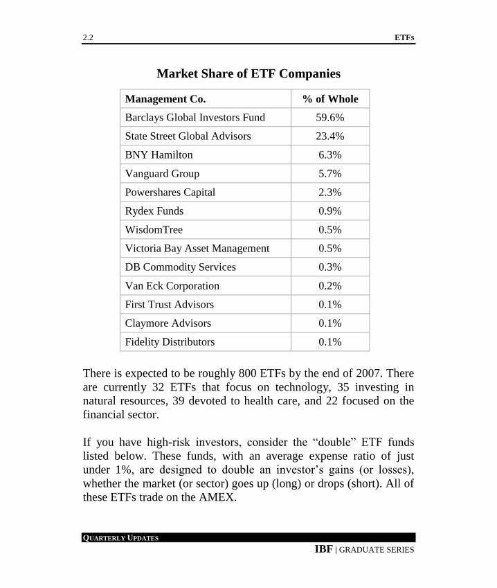
The next table shows the largest ETF management companies. The
percentage figures indicate the percentage of the entire ETF
marketplace managed by each company; Barclays oversees just
under 60% of the entire ETF industry assets.
2.2 ETFS
QUARTERLY UPDATES
IBF | GRADUATE SERIES
Market Share of ETF Companies
Management Co. % of Whole
Barclays Global Investors Fund 59.6%
State Street Global Advisors 23.4%
BNY Hamilton 6.3%
Vanguard Group 5.7%
Powershares Capital 2.3%
Rydex Funds 0.9%
WisdomTree 0.5%
Victoria Bay Asset Management 0.5%
DB Commodity Services 0.3%
Van Eck Corporation 0.2%
First Trust Advisors 0.1%
Claymore Advisors 0.1%
Fidelity Distributors 0.1%
There is expected to be roughly 800 ETFs by the end of 2007. There
are currently 32 ETFs that focus on technology, 35 investing in
natural resources, 39 devoted to health care, and 22 focused on the
financial sector.
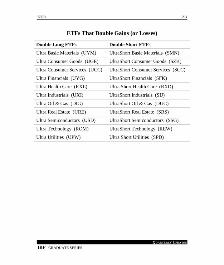
If you have high-risk investors, consider the “double” ETF funds
listed below. These funds, with an average expense ratio of just
under 1%, are designed to double an investor’s gains (or losses),
whether the market (or sector) goes up (long) or drops (short). All of
these ETFs trade on the AMEX.
ETFS 2.3
QUARTERLY UPDATES
IBF | GRADUATE SERIES
ETFs That Double Gains (or Losses)
Double Long ETFs Double Short ETFs
Ultra Basic Materials (UYM) UltraShort Basic Materials (SMN)
Ultra Consumer Goods (UGE) UltraShort Consumer Goods (SZK)
Ultra Consumer Services (UCC) UltraShort Consumer Services (SCC)
Ultra Financials (UYG) UltraShort Financials (SFK)
Ultra Health Care (RXL) Ultra Short Health Care (RXD)
Ultra Industrials (UXI) UltraShort Industrials (SIJ)
Ultra Oil & Gas (DIG) UltraShort Oil & Gas (DUG)
Ultra Real Estate (URE) UltraShort Real Estate (SRS)
Ultra Semiconductors (USD) UltraShort Semiconductors (SSG)
Ultra Technology (ROM) UltraShort Technology (REW)
Ultra Utilities (UPW) Ultra Short Utilities (SPD)
2.4 ETFS
QUARTERLY UPDATES
IBF | GRADUATE SERIES
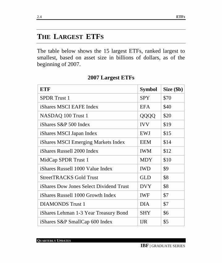
THE LARGEST ETFS
The table below shows the 15 largest ETFs, ranked largest to
smallest, based on asset size in billions of dollars, as of the
beginning of 2007.
2007 Largest ETFs
ETF Symbol Size ($b)
SPDR Trust 1 SPY $70
iShares MSCI EAFE Index EFA $40
NASDAQ 100 Trust 1 QQQQ $20
iShares S&P 500 Index IVV $19
iShares MSCI Japan Index EWJ $15
iShares MSCI Emerging Markets Index EEM $14
iShares Russell 2000 Index IWM $12
MidCap SPDR Trust 1 MDY $10
iShares Russell 1000 Value Index IWD $9
StreetTRACKS Gold Trust GLD $8
iShares Dow Jones Select Dividend Trust DVY $8
iShares Russell 1000 Growth Index IWF $7
DIAMONDS Trust 1 DIA $7
iShares Lehman 1-3 Year Treasury Bond SHY $6
iShares S&P SmallCap 600 Index IJR $5

ETFS 2.5
QUARTERLY UPDATES
IBF | GRADUATE SERIES
ETFS WITH LOW EXPENSE RATIOS
The table below shows the 15 lowest expense ratio ETFs, as of
the beginning of 2007.
2007 Lowest Expense Ratio ETFs
ETF Symbol Expense
Vanguard Large Cap VV 0.09
iShares S&P 500 Index IVV 0.09
SPDR Trust 1 SPY 0.10
iShares Lehman 7-10 Year Treasury Bond IEF 0.15
iShares iBoxx $ Invest. Grade Corp. Bond LQD 0.15
iShares Lehman 1-3 Year Treasury Bond TIP 0.15
iShares Lehman 20+ Year Treasury Bond TLT 0.15
iShares Russell 1000 Index IWB 0.15
DIAMONDS Trust 1 DIA 0.17
iShares S&P 500 Growth Index IVW 0.18
iShares S&P 500 Value Index IVE 0.18
NASDAQ 100 Trust 1 QQQQ 0.20
iShares Lehman Aggregate Bond AGG 0.20
iShares Lehman TIPS Bond TIP 0.20
iShares NYSE 100 Index NY 0.20

2.6 ETFS
QUARTERLY UPDATES
IBF | GRADUATE SERIES
ETF PRICE DISPARITIES
Often times, some of the most actively traded issues on the NYSE
and other U.S. markets are ETFs. Barclays estimates that on any
given day, 80% of the trading of its ETFs are traded by large
investors such as hedge funds. As of May 2007, there were about
500 ETFs in the U.S., valued at $500 billion (vs. 8,100 traditional
mutual funds valued at $10.5 trillion). Although ETFs are expected
to closely track an underlying index, this is not always the case
during extreme days in the market.
For example, on February 27th
, 2007, an ETF managed by Barclays
that tracks the Chinese stock market closed down 9.9% in the U.S.,
even though the underlying index had fallen 2.1% during Chinese
trading hours. The index fell an additional 3.1% the next day in
China (but the Barclay’s iShares rose 4.3%). However, had U.S.
investors sold the Barclays ETF just before the close of trading on
February 27th
, their loss would have been 9.9%, not the actual loss of
the index, 2.1%. On the positive side, purchasers of the Barclays
ETF would have bought at a 7.8% discount (9.9% - 2.1%), resulting
in a substantial gain for owning the ETF shares for less than a day.
Another example is the precious metals ETF offered by Powershares
Capital Management. On Februrary 27th
, the ETF ended the day
3.3% below the actual value of the fund’s holdings. The iShares
emerging markets ETF lost 8.1%, even though the index was down
just 3.1%. As a result, a seller of $10,000 of the Barclay’s iShares
would have received $500 less than if the fund had actually tracked
the index.

ETFS 2.7
QUARTERLY UPDATES
IBF | GRADUATE SERIES
There are disparities even for ETFs that track just U.S. stocks. The
Russell 2000 Index (small company stocks) fell 3.75% on February
27th
, 2007, versus 4.70% for the actual index. In this case, a large
part of the disparity (almost 1%) was because like other ETFs, this
Russell ETF trades for 15 minutes longer than regular stocks. For all
of February 27th
, 89 of the 421 ETFs tracked by Morningstar fell
short of their portfolio value by more than 1% (+/-1/2% is considered
normal). Of those 89 ETFs, 60 fell short by more than 2%.
There are three lessons to be learned from these index and ETF
disparities. First, when there is a panic, the pricing of a number of
ETFs can be quite different than the underlying index (somewhat
similar to the premium-discount difference with most closed-end
funds). Second, advisors should think twice about selling any
investment, and in particular an ETF or CEF, during periods of high
short-term volatility. Third, it is extremely likely that any disparity,
no matter how narrow or wide, is likely to be corrected within one or
two days, thereby making moot any attempt to sensationalize such
price differences.
SECTOR VOLATILITY
The most volatile sector ETFs are, from highest to lowest risk, are:
1. Technology 6. Materials
2. Financial (includes REITs) 7. Energy
3. Healthcare 8. Consumer Staples
4. Consumer Discretionary 9. Utilities
5. Industrial

2.8 ETFS
QUARTERLY UPDATES
IBF | GRADUATE SERIES
BUYING AND SELLING ETFS
The majority of all stock and ETF trades are:
1. Market order—You get the best price currently available;
most orders are market orders.
2. Limit order—You place a buy order, indicating that you are
willing to pay $X per share or less. If you place a sell limit
order, you are indicating that you want $Y per share or more.
If someone is not willing to sell you shares for $X or less, the
order is not filled; similarly, if someone is not willing to buy
your shares for $Y or more, you will end up not selling the
shares.
3. Stop-loss (or stop) order—The order goes into effect as soon
as the price per share of the stock (or ETF) hits a certain
price. Once this price is reached, the stop-loss order becomes
a market order. This type of order is frequently used to limit
price declines if the security’s price falls.
4. Short sale—You believe the price per share of a stock or
ETF is going to fall. Shares of a stock or ETF are borrowed
by your brokerage firm on your behalf (note: you will be
paying an ongoing interest charge for the borrowing). If the
price of the security falls after the short sale, you have a gain;
if the price of the security rises, you have a loss. At some
point in the future, the investor will decide to buy the stock or
ETF and thereby repay the original borrowed shares.

QUARTERLY
UPDATES
UITS AND
CLOSED-END FUNDS


UITS AND CLOSED-END FUNDS 3.1
QUARTERLY UPDATES
IBF | GRADUATE SERIES
3.UIT AND NEW FUND CRITICISM
Some newly launched mutual funds as well as UITs rely on
historical data to increase sales and help market their portfolios.
Critics argue that these new offerings simply keep shifting the
composition of the funds’ proposed holdings until they find one that
happens to have worked over the necessary range of dates.
CLOSED-END FUND ASSET INCREASE
For the first quarter of 2007, more than $13 billion was raised
through closed-end fund IPOs, more than was raised for all of 2006.
At the end of 2006, the closed-end fund (CEF) industry managed
$420 billion in assets. As of the end of the first quarter of 2007, the
median discount for all CEFs was 2.3%; about 35% of all CEFs
trade at a premium over their NAV.
CEF IPOs
Year # of IPOs $ (billions)
2006 21 $11
2005 47 $21
2004 50 23
2003 48 28
2002 77 16

3.2 UITS AND CLOSED-END FUNDS
QUARTERLY UPDATES
IBF | GRADUATE SERIES
A number of sources believe that CEF IPOs are not good for
investors since the majority of them end up trading at a discount
to NAV. These same critics believe that the IPO market for CEFs
largely rely on unsophisticated income-oriented investors. In January
2007, the IPO for Alpine Total Dynamic Dividend Fund raised over
$4 billion.
CLOSED-END COVERED CALL FUNDS
Closed-end covered-call funds have the objective of generating high
income by selling call options on stocks in their portfolios. These
types of funds first appeared in 2004 and accounted for 85% of IPO
money going into closed-end funds. Even though these are equity
funds, a number of analysts consider them to be a “fixed-income
application.”
The goal of a closed-end covered-call fund manager is to achieve the
highest premium income possible while forfeiting the least amount
of equity upside. Critics feel that these funds cap returns in bull
markets (since good-performing stocks will be called away), and in a
crash or severe correction do not generate enough option-writing
income to offset the decline. In some respects, these funds perform
best, at least comparatively speaking, when the market is flat or
rising slightly.
The Chicago Board Options Exchange (CBOE) currently licenses
four buy-write indexes. The table below lists the six largest closed-
end covered-call funds. As of the third quarter of 2006, all six of
these funds were selling at a discount that ranged from 3% to 9%.

UITS AND CLOSED-END FUNDS 3.3
QUARTERLY UPDATES
IBF | GRADUATE SERIES
The Largest Closed-End Covered-Call Funds
NFJ Dividend, Interest &
Premium Strategy
Nuveen Equity Premium
Opportunity
Eaton Vance Tax-Managed
Global Buy-Write
Eaton Vance Tax-Managed Buy-
Write Opportunity
ING Global Equity Dividend &
Premium Opportunity
Black Rock Enhanced Dividend
Achievers

QUARTERLY
UPDATES
REITS


REITS 4.1
QUARTERLY UPDATES
IBF | GRADUATE SERIES
4.REIT UPDATE
After stagnating in 1999, real estate funds went on to average just
under 22% per year for the next seven years (ending 12/31/2006).
This sector category can also provide diversification, when the S&P
500 dropped 9% in 2000, real estate funds gained 27%. The table
below shows return figures for REIT sectors, as of March 1st, 2007.
REIT Sector Returns [ending 3-1-2007]
REIT category 1-year 3-year 5-year 10-year
Apartments 24.1% 29.6% 21.7% 15.9%
Regional Malls 30.8% 28.4% 33.9% 21.4%
Shopping Centers 34.7% 26.7% 29.1% 18.5%
Office Buildings 41.7% 27.3% 22.3% 15.4%
Industrial 24.8% 25.8% 26.0% 17.2%
Health Care 41.1% 18.3% 23.1% 14.9%
Self Storage 29.7% 30.8% 25.6% 18.0%
Lodging / Resorts 24.5% 24.4% 17.1% 5.3%
Manufactured Homes 8.7% 3.4% 8.2% 9.1%
Mortgage REIT Index 7.2% -4.6% 15.1% 6.6%

4.2 REITS
QUARTERLY UPDATES
IBF | GRADUATE SERIES
INTERNATIONAL REITS
From 2003 to 2007, Asia REITs returned an average of 35.4% per
year; 43.5% annually in the case of European REITs (67% in 2006).
In the U.S. there are about 180 REITs registered with the SEC. Japan now has more than 40. Over 20 countries have passed or
considered laws allowing the formation of REITs. The U.K. and
Germany adopted REIT laws in early 2007.

QUARTERLY
UPDATES
STOCKS


STOCKS 5.1
QUARTERLY UPDATES
IBF | GRADUATE SERIES
5.DOW MILESTONES
The Dow Jones Industrial Average (DJIA) began with just 12 stocks
in 1896 when the average had a starting value of 40.94. Since 1928,
there have been 30 stocks in the Dow. The table below shows Dow
milestones.
It took 127 days for the DJIA to move from 12,000 to 13,000. In
1999, it took 24 days to move from 10,1000 to 11,000. But it took
7.5 years to move from 11000 to 12,000. The Great Depression
caused the DJIA to lose 90% of its value. The high it reached on
September 3rd
, 1929, was not surpassed until 1954.
The Dow Hitting 1,000 Point Increments
Dow Date Dow Date
12000 Oct. 19, 2006 5000 Nov 21, 1995
11000 May 3, 1999 4000 Feb 23, 1995
10000 March 29, 1999 3000 Apr. 17, 1991
9000 April 6, 1998 2000 Jan. 8, 1987
8000 July 16, 1997 1000 Nov. 14, 1972
7000 Feb. 13, 1997 start May 26, 1896
6000 Oct 14, 1996

5.2 STOCKS
QUARTERLY UPDATES
IBF | GRADUATE SERIES
DOW DROPS
The table below shows the biggest percentage drops in the Dow
Jones Industrial Average (DJIA) from the beginning of 2003 to
March 17th, 2007. Since 1980, the return on the DJIA has averaged
13.9% per year, versus 13.1% for the S&P 500. There are 10 sectors
in the S&P 500:
DJIA Biggest 1-Day Drops [1-1-2003 through 3-17-2007]
Date % Change Date % Change
3-24-03 3.6% 5-19-03 2.1%
2-27-07 3.3% 1-30-03 2.0%
1-24-03 2.9% 3-13-07 2.0%
3-10-03 2.2%
S&P 500 Sectors
consumer discretionary industrials
consumer staples materials
energy technology
financials telecom
health care utlities
If the technology sector were excluded from the S&P 500, the S&P
500 would be 16% above its 2000 peak. Looking at the entire S&P
500 (including technology stocks), more than 2/3 of the stocks are
above their peak prices reached in 2000.

STOCKS 5.3
QUARTERLY UPDATES
IBF | GRADUATE SERIES
S&P 500 AND DJIA RETURNS
As of May 3rd
, 2007, the S&P 500 was within 2% of its record close
of 1527.5 in March 2000. On the same day, the Dow Jones Industrial
Average (DJIA) hit another all-time record for 2007, closing at
13,241.4. The NASDAQ, which closed at 2,565.5, is still roughly
50% below its 2000 all-time high of over 5,000.
50TH
ANNIVERSARY OF THE S&P 500
From its March 1st, 1957 inception through the end of 2006, the
average annual return of the S&P 500 has been 10.83%. The S&P
500 comprises 83% of the value of all U.S. stocks. Almost 1,000
new companies have been added and deleted from the index since its
inception.
The materials and energy sectors made up half the value of the
original index, compared to 12% in 2007. By a wide margin, the best
performing stock has been Altria (formally Phillip Morris); from
March 1957 through the end of 2006, investors averaged 19.9%
annually. A $10,000 investment grew to $8.4 million (vs. $168,000
if the $10,000 had been invested in the entire index). Of the original
111 surviving companies, 20 outperformed the index by an average
of almost 5% per year.

5.4 STOCKS
QUARTERLY UPDATES
IBF | GRADUATE SERIES
SMALL CAP STOCKS
U.S. small company stocks with market capitalizations of less than
$3.5 billion have averaged 16.5% a year versus 12.2% for the S&P
500 over the past 30 years (ending 6/30/2006). As of the beginning
of 2007, small cap companies represented 78% of all listed
stocks in the U.S. (84% in Japan, 79% in Hong Kong, 74% in the
U.K. and 65% in France).
QUALIFYING DIVIDENDS
Legislation passed in 2004 cut the tax rate on “qualifying” dividends
to a maximum of 15%. For investors, “qualified” means that the
stock (paying the dividend) has to be owned by both the investor and
the mutual fund or ETF for at least 61 of the 121 days surrounding
the ex-dividend date. Income paid out by REITs and some overseas
companies do not qualify for this lower rate.
BUFFET WARNING
During the May 2007 Berkshire Hathaway annual meeting, Warren
Buffet repeated his warning about derivatives and leverage. Buffet
believes that derivatives are the “financial weapons of mass
destruction.” He expects that derivatives and the use of leverage by
traders, investors, and corporations will eventually end in huge
losses. According to Buffet, “The introduction of derivatives has
totally made any regulation of margin requirements a joke.”

STOCKS 5.5
QUARTERLY UPDATES
IBF | GRADUATE SERIES
DIVIDEND-PAYING BONUS
According to a Morgan Stanley report, from 1970 through 2005,
stocks that paid dividends averaged annual returns of 10.2%,
almost six percentage points ahead of non-payers. According to
S&P, 383 companies in the S&P 500 paid dividends in 2006,
compared with 351 in 2001. A decade ago, 427 out of 500 paid
dividends. The average payout ratio is just below 32%. Morgan
Stanley estimates that 40% of the S&P 500’s annual total returns
were from dividends for the period 1926 through 2004. Standard &
Poor’s reports that approximately one out of every nine stocks (59
total) in the S&P 500 has increased its annual dividend for at least 25
consecutive years as of the end of 2006.
VALUE PLAY
Suppose you wanted to buy a quart of milk. Last week you
bought a quart for $1.20. This week it is selling for $13.00 a
quart. How likely is it that you would buy a $13 quart of milk?
Yet, when it comes to buying stock, no one asks what the
“quart” (stock) used to sell for.
From the beginning of 2000 to the end of 2006, the average large
cap value fund had a cumulative return of just under 60%, versus
just 18% for the typical large cap growth fund. The Russell 1000
Value Index was up 22% in 2006, but only 6% of active large cap
value managers beat the index. Even though financial stocks
currently comprise 36% of the Russell 1000 Value Index, few active
money managers will devote that much to financials or any other
single sector.


QUARTERLY
UPDATES
VALUE VS.
GROWTH STOCKS


VALUE VS. GROWTH STOCKS 6.1
QUARTERLY UPDATES
IBF | GRADUATE SERIES
6.ROLLING PERIODS: GROWTH VS. VALUE
The table below shows the number of positive rolling three-year
periods, for different growth and value categories over the past 30
years, ending December 31st, 2006. Over a 30-year period, there are
28, three-year rolling periods.
Positive 3-Year Rolling Periods,
Growth vs. Value Stocks [1977-2006]
Category + Returns % +
Large Growth 25 / 28 yrs. 89%
Large Value 26 / 28 yrs. 93%
Mid Growth 27 / 28 yrs. 96%
Mid Value 28 / 28 yrs. 100%
Small Growth 27 / 28 yrs. 96%
Small Value 28 / 28 yrs. 83%
ALL GROWTH 25 / 28 yrs. 89%
ALL VALUE 26 / 28 yrs. 93%
The table below shows the number of positive rolling five-year
periods, for different growth and value categories over the past 30
years, ending December 31st, 2006. Over a 30-year period, there are
26, five-year rolling periods.

6.2 VALUE VS. GROWTH STOCKS
QUARTERLY UPDATES
IBF | GRADUATE SERIES
Positive 5-Year Rolling Periods,
Growth vs. Value Stocks [1977-2006]
Category + Returns % +
Large Growth 22 / 26 yrs. 85%
Large Value 25 / 26 yrs. 96%
Mid Growth 24 / 26 yrs. 92%
Mid Value 26 / 26 yrs. 100%
Small Growth 24 / 26 yrs. 92%
Small Value 26 / 26 yrs. 100%
ALL GROWTH 22 / 26 yrs. 85%
ALL VALUE 25 / 26 yrs. 96%
In summary, looking at both tables in this section, almost all of the
negative annual returns took place during the 2000-2002 stock
market meltdown. In the case of three- and five-year rolling periods,
all negative periods were the result of the same meltdown.
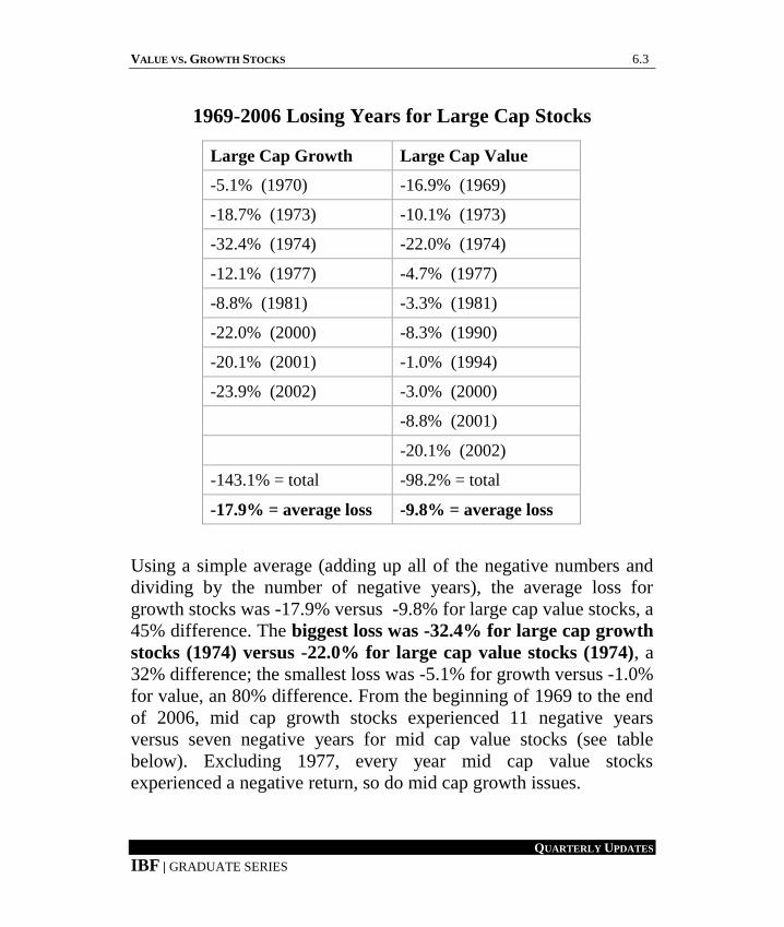
REVISITING GROWTH AND VALUE
From the beginning of 1969 to the end of 2006, large cap growth
stocks experienced eight negative years versus 10 negative years for
large cap value stocks (see table below). Excluding 1970, every
year large cap growth stocks experienced a negative return, so
did large cap value issues.
VALUE VS. GROWTH STOCKS 6.3
QUARTERLY UPDATES
IBF | GRADUATE SERIES
1969-2006 Losing Years for Large Cap Stocks
Large Cap Growth Large Cap Value
-5.1% (1970) -16.9% (1969)
-18.7% (1973) -10.1% (1973)
-32.4% (1974) -22.0% (1974)
-12.1% (1977) -4.7% (1977)
-8.8% (1981) -3.3% (1981)
-22.0% (2000) -8.3% (1990)
-20.1% (2001) -1.0% (1994)
-23.9% (2002) -3.0% (2000)
-8.8% (2001)
-20.1% (2002)
-143.1% = total -98.2% = total
-17.9% = average loss -9.8% = average loss
Using a simple average (adding up all of the negative numbers and
dividing by the number of negative years), the average loss for
growth stocks was -17.9% versus -9.8% for large cap value stocks, a
45% difference. The biggest loss was -32.4% for large cap growth
stocks (1974) versus -22.0% for large cap value stocks (1974), a
32% difference; the smallest loss was -5.1% for growth versus -1.0%
for value, an 80% difference. From the beginning of 1969 to the end
of 2006, mid cap growth stocks experienced 11 negative years
versus seven negative years for mid cap value stocks (see table
below). Excluding 1977, every year mid cap value stocks
experienced a negative return, so do mid cap growth issues.

6.4 VALUE VS. GROWTH STOCKS
QUARTERLY UPDATES
IBF | GRADUATE SERIES
1969-2006 Losing Years for Mid Cap Stocks
Mid Cap Growth Mid Cap Value
-13.6% (1969) -18.6% (1969)
-6.4% (1970) -15.7% (1973)
-32.5% (1973) -20.9% (1974)
-33.1% (1974) -1.0% (1987)
-3.1% (1981) -15.6% (1990)
-6.1% (1984) -1.7% (1994)
-5.1% (1990) -12.8% (2002)
-2.3% (1994)
-18.5% (2000)
-7.2% (2001)
-21.5% (2002)
-149.2% = total -86.3% = total
-13.6% = average loss -12.3% = average loss
Using a simple average (adding up all of the negative numbers and
dividing by the number of negative years), the average loss for
growth stocks was -13.6% versus -12.3% for value stocks, a 10%
difference. The biggest loss was -33.1% for mid cap growth stocks
(1974) versus -20.9% for mid cap value stocks (1974), a 63%
difference; the smallest loss was -2.3% for growth versus -1.7% for
value, a 26% difference.

VALUE VS. GROWTH STOCKS 6.5
QUARTERLY UPDATES
IBF | GRADUATE SERIES
From the beginning of 1969 to the end of 2006, small cap growth
stocks experienced 11 negative years versus eight negative years
for small cap value stocks (see table below). Excluding 1998, every
year small cap value stocks experienced a negative return, so do
small cap growth issues.
1969-2006 Losing Years for Small Cap Stocks
Small Cap Growth Small Cap Value
-19.6% (1969) -19.1% (1969)
-13.7% (1970) -24.4% (1973)
-40.6% (1973) -20.4% (1974)
-28.9% (1974) -4.7% (1987)
-4.9% (1981) -18.7% (1990)
-7.4% (1984) -0.1% (1994)
-7.9% (1987) -4.1% (1998)
-16.3% (1990) -13.3% (2002)
-1.9% (1994)
-22.6% (2000)
-27.8% (2002)
-191.6% = total -104.8% = total
-17.4% = average loss -13.1% = average loss

6.6 VALUE VS. GROWTH STOCKS
QUARTERLY UPDATES
IBF | GRADUATE SERIES
Using a simple average (adding up all of the negative numbers and
dividing by the number of negative years), the average loss for
growth stocks was -17.4% versus -13.1% for value stocks, a 25%
difference. The biggest loss was -40.6% for small cap growth
stocks (1973) versus -24.4% for small cap value stocks (1973), a
40% difference; the smallest loss was -1.9% for growth versus -
0.1% for value, a 95% difference.
Conclusions Whether the comparison is between large, mid, or small cap
issues, value has suffered less than growth from 1969 through
2006; the average loss has been smaller. The largest losses were
always in growth and the smallest losses were always in value
stocks. In the case of mid and small cap stocks, the frequency of
losses has been greater for growth.
Adding up the cumulative returns of growth versus value from
1969 to the end of 2006, value has dramatically outperformed
growth (as shown in the table below); large value outperformed
large growth by almost 2-1, over 3-1 in the case of mid cap value
versus mid cap growth, and over 7-1 in the case of small cap
value versus small cap growth. As a side note, the standard
deviation for large, mid, and small cap value stocks has been
lower than their growth counterparts in the 1970s, 1980s, 1990s,
2000s, and from 1997 through 2006.

VALUE VS. GROWTH STOCKS 6.7
QUARTERLY UPDATES
IBF | GRADUATE SERIES
Growth of $10,000 from 1969 to the end of 2006
LC
Growth
LC
Value
MC
Growth
MC
Value
SC
Growth
SC
Value
$276,070 $539,470 $342,940 $1,429,090 $276,970 $2,338,810
From the beginning of 1928 through the end of 2006, $10,000
invested in small cap value stocks grew to $549,670,000 versus
$13,710,000 for small cap growth stocks (a margin of 39 to 1).
The same dollar invested in large cap value stocks grew to
$76,620,000 versus $9,740,000 for large cap growth stocks (a
margin of 6.7 to 1). Surprisingly, from 1928 through 2006, the
standard deviation for small cap value stocks was only slightly lower
than it was for small cap value stocks; the large cap growth stocks
has less risk (standard deviation of 20) than large cap value stocks
(standard deviation of 27) during the same period
SMALL CAP VALUE
Dartmouth finance professor Kenneth French and University of
Chicago economics professor Eugene Fama, who founded
Dimensional Fund Advisors (DFA) in 1981, developed the “Three
Factor Model” that questioned the validity of William Sharpe’s
capital asset pricing model (CAPM). DFA believes that tilting a
portfolio towards value and small cap stocks leads to better
performance over time. According to their historical studies, value
has outperformed growth by 5.1% annually since 1927.

6.8 VALUE VS. GROWTH STOCKS
QUARTERLY UPDATES
IBF | GRADUATE SERIES
GROWTH VS. VALUE
The table below shows the number of positive annual returns for
different growth and value categories over the past 30 years, ending
December 31st, 2006.
Positive Annual Returns
Growth vs. Value Stocks [1977-2006]
Category + Returns % +
Large Growth 25 / 30 yrs. 83%
Large Value 23 / 30 yrs. 77%
Mid Growth 23 / 30 yrs. 77%
Mid Value 26 / 30 yrs. 87%
Small Growth 22 / 30 yrs. 73%
Small Value 25 / 30 yrs. 83%
ALL GROWTH 24 / 30 yrs. 80%
ALL VALUE 25 / 30 yrs. 83%

VALUE VS. GROWTH STOCKS 6.9
QUARTERLY UPDATES
IBF | GRADUATE SERIES
2006 INDEX RETURNS
The tables below show returns for nine major indexes and the 10
Dow Jones industry groups for the 2006 calendar year.
2006 Index Returns
Index Return Index Return
DJIA 16.3% AMEX 16.9%
DJ World (excl. U.S.) 23.0% S&P 500 13.6%
DJ Wilshire 5000 13.9% Value Line 11.0%
NYSE Composite 17.9% NASDAQ 9.5%
Russell 2000 17.0%
2006 Dow Jones Industry Group Returns
Industry Group Return Industry Group Return
Basic Materials 16.1% Industrials 12.7%
Consumer Goods 12.5% Oil & Gas 20.3%
Consumer Services 13.5% Technology 9.5%
Financials 16.5% Telecommunications 32.2%
Health Care 5.7% Technology 9.5%


QUARTERLY
UPDATES
BONDS


BONDS 7.1
QUARTERLY UPDATES
IBF | GRADUATE SERIES
7.CUSHION AGAINST STOCK DECLINES
The table below shows the benefit of owning tax-free bonds during
stock market declines. From1986-2006, there have been four
instances when the S&P 500 has declined by 15% or more.
S&P 500 Decline
(high to low)
S&P 500
(with dividends)
Lehman Brothers
Municipal Bond Index
8-25-87 to 12-4-87 - 32.8% - 0.8%
7-16-90 to 10-11-90 - 19.2% - 1.4%
7-17-98 to 8-31-98 - 19.1% 1.8%
3-24-00 to 10-9-02 - 47.4% 25.1%
STOCKS VS. BONDS
Even though the 2000-2002 bear market represents the worst
cumulative drop in the S&P 500 over the past 50 years (-49%),
stocks still did better than bonds for the 10-year period ending
December 31st, 2006 (124% for the S&P 500 vs. 83% for the
Lehman Brothers Aggregate bond index).

7.2 BONDS
QUARTERLY UPDATES
IBF | GRADUATE SERIES
2006 HIGH-YIELD BOND FACTS
In 1980, slightly less than a third of U.S. industrial corporations
tracked by Standard & Poor’s were rated junk. By the late 1980s,
more than half were; the number increased to 71% by early 2007.
The S&P 500 includes 70 companies whose bonds are rated below
investment grade.
During the past 20 years, 4.5% of junk bonds have gone into default;
in 1991 and 2002, defaults were more than 10% of outstanding high-
yield bonds. The default rate was just 1.3% for 2006 (only 0.8%
according to Fitch). The table below shows that the number of
companies with high-risk credit ratings (BB or lower) has jumped
since 1980 (note: the table does not include utilities or financial
institutions).
Corporate Bond Ratings in 2006 vs. 1980
S&P Rating 1980 2006
AAA/AA 17% 2%
A 33% 9%
BBB 18% 18%
BB 22% 25%
B 7% 42%
CCC/D 3% 4%

BONDS 7.3
QUARTERLY UPDATES
IBF | GRADUATE SERIES
According to the Financial Times, 1.6% of global junk bond debt
defaulted in 2006; this is the lowest default rate experienced by
global junk bonds since 1981. The historical default rate for junk
bonds is 4.9% annually.
BOND MARKETS, INDEXES, AND FUNDS
The U.S. bond market more than doubled from $10.7 trillion in 1996
to $22.7 trillion by the middle of 2006. The Lehman Brothers
Aggregate Bond Index is comprised of more than 7,000 different
bonds, many of which are illiquid that fund managers cannot buy,
even if they wanted to. However, by copying some of the index’s
broad characteristics, such as sector exposure, interest rate
sensitivity and maturity, bond fund managers can end up with
portfolios that are very similar to the Lehman index.
Indices and averages are cost-free in the sense that their structure
and performance do not include any initial or ongoing costs such as
commissions, management fees, or bid-ask spreads. Since a mutual
fund incurs all of these costs, it can only beat an index by being
different. In the case of bond funds, increased credit risk, yield-curve
positioning, or emphasizing sectors or issues different from the
index are the only ways to outperform.

7.4 BONDS
QUARTERLY UPDATES
IBF | GRADUATE SERIES
R-squared reflects the percentage change of a fund’s fluctuation
that can be explained by the change in its benchmark index. A
fund that highly corresponds to its respective index has an R-squared
in the high 80s or 90s. For the 10-year period ending September
2006, only two of 15 funds with 10-year R-squareds of 98 or higher
outperformed the Lehman Brothers Aggregate Bond Index. Fund
expenses prevented the other 13 possible candidates from
outperforming the index. However, over the past three and five
years, the following funds have been able to outperform the Lehman
index even after taking into account trading costs and expenses:
Metro West Total Return, Dodge & Cox Income, Western Asset
Credit Bond Institutional, Fidelity Mortgage Security, TCW Total
Return Bond I, Harbor Bond Institutional, Fidelity Total Bond,
Managers Fremont Bond, PIMCO Total Return D, T. Rowe Price
New Income, USAA Income, and Fidelity Investment Grade Bond.
All of these funds had an R-squared of 94 or higher, with the
exception of Dodge & Cox Income (R-squared of 91) and Metro
West Total Return (R-squared of 69).
Obviously, funds that try to match a bond index’s performance are
going to fail if their expense ratios are too high. The advisor who is
seeking index-type returns will have to either choose low expense
funds or portfolio’s that have securities different than their
respective index—specifically, high-yield issues.

BONDS 7.5
QUARTERLY UPDATES
IBF | GRADUATE SERIES
Defaults on U.S. junk bonds for the 2006 calendar year were 1.3%,
well below the historical average of 4.5%, as computed by Standard
& Poor’s. Another respected rating service, Fitch, shows the 2006
default rate at just 0.8%, down from 3.1% in 2005 and well below
the long-term average of 5.0%. Over the past 10 years, the yield
spread between high-yield corporate debt and U.S. Treasuries has
been as low as 2.6% (early 2007) and higher than 10.0% (fall of
2002). Thus, in the current environment, your clients may be able to
outperform an index bond fund by focusing on low-cost funds that
have the flexibility to increase their exposure to high-yield.
Before discounting the importance of bonds, consider the following:
From January 1st, 2000 to December 31
st, 2002, a $100,000
investment in the S&P 500 fell to $62,406 while a $100,000
investment in the Lehman Brothers Aggregate Bond Index grew to
$133,466.


QUARTERLY
UPDATES
GLOBAL INVESTING


GLOBAL INVESTING 8.1
QUARTERLY UPDATES
IBF | GRADUATE SERIES
8.WORLD’S FINANCIAL ASSETS
As of the beginning of 2006, the value of the world’s financial
assets was over $140 trillion. This figure is three times as large as
the total output of goods and services produced around the globe.
Flows of investment across borders hit $6 trillion in 2005.
Of all the savings that people are willing to invest outside their
country, the U.S. gets 85%. Worldwide, about one in five stocks
is owned by someone who lives outside the country where the
stock was issued. The table below shows financial assets for
countries and regions at the beginning of 2005, in trillions of U.S.
dollars.
World Assets as of 1-1-2006 [in trillions of U.S. dollars]
Area $ (t) Area $ (t)
U.S. $48 Australia, New Zealand, & Canada $5
Euro Area $27 Other Western Europe $4
Japan $17 Latin America $3
Emerging Asia $10 Hong Kong & Singapore $2
U.K. $7 Eastern Europe $2

8.2 GLOBAL INVESTING
QUARTERLY UPDATES
IBF | GRADUATE SERIES
EMERGING MARKET DEBT
In 1997, emerging market government debt was $786 billion; by the
end of 2006, the figure was $3.15 trillion. Corporations in those
countries had $416 billion of home-currency debt in 1997, versus
$1.4 trillion by the end of 2006.
2006 GLOBAL INDEX RETURNS
The tables below show returns for Dow Jones global indexes in 2006
in U.S. dollars and in local currency.
2006 Dow Jones Global Index Returns
Country U.S. $ Local Country U.S. $ Local
Venezuela 63% 111% Mexico 39% 42%
Indonesia 62% 48% Singapore 39% 28%
Philippines 49% 38% Austria 38% 24%
Spain 47% 31% Hong Kong 38% 39%
Sweden 43% 23% Germany 35% 21%
Norway 43% 32% Greece 35% 21%
Ireland 42% 27% Denmark 34% 20%
Portugal 42% 27% France 34% 20%
Brazil 42% 30% Malaysia 33% 24%

GLOBAL INVESTING 8.3
QUARTERLY UPDATES
IBF | GRADUATE SERIES
2006 Dow Jones Global Index Returns
Country U.S. $ Local Country U.S. $ Local
Belgium 32% 18% South Africa 18% 31%
Italy 31% 17% Canada 16% 16%
Chile 30% 36% South Korea 15% 6%
Netherlands 30% 16% U.S. 14% 14%
Finland 28% 15% New Zealand 13% 9%
Australia 28% 19% Thailand 6% -6%
U.K. 28% 12% Japan 2% 3%
Switzerland 27% 18% World 19%
Taiwan 21% 20%
Greater China has two major exchanges, the Shanghai and the
Shenzhen. For 2006, China’s Shanghai A Shares increased 131% in
local currency (96% in the case of Shenzhen A shares).
REDUCED GLOBAL CORRELATION
For the two-year period ending February 2007, correlation between
U.S. and other developed markets was 0.63, according to ING Asset
Management. From 2003 to 2005, the correlation was an incredibly
high 0.93 (S&P 500 vs. EAFE). Bear Sterns believes that these very
high correlations were due to the bursting of the tech bubble.

8.4 GLOBAL INVESTING
QUARTERLY UPDATES
IBF | GRADUATE SERIES
EAFE COMPOSITION
Five countries, France, Germany, Japan, Switzerland, and the
U.K., comprise 70% of the EAFE index; Japan alone represents
22% of the index. Over the past 10 years (ending 12/31/2006),
Japanese stocks have averaged 2.3% in U.S. dollar terms.
The S&P 500 and EAFE index have either both risen or fallen in
the same calendar year for each of the last 14 consecutive years
(1993-2006); however, during the same period, the spread between
the two indexes averaged 13% per year.
As of the beginning of March 2007, the EAFE Index was divided as
follows: Japan (23%), the U.K. (23%), France (10%), Germany
(7.5%), Switzerland (7%), and Asia ex-Japan (8.5%). The market
capitalization of the typical stock in the EAFE is $33 billion; 57%
of the index is comprised of “giant” stocks, 33% large stocks, 11%
medium, and 0.1% small stocks.
The market capitalization of the roughly 1,400 stocks in the
EAFE is $10.2 trillion. The largest stock in the index is British
Petroleum, which has a market capitalization of over $220 billion.
The only Japanese stock in the top 10 is Toyota, ranked number
three (1.5% of the index). Of the top seven companies, five are from
the U.K. Over half the stocks in the portfolio are classified as either
financials, consumer discretionary, or industrial issues. The table
below shows the composition of the MSCI EAFE Index as of the
beginning of 2006.

GLOBAL INVESTING 8.5
QUARTERLY UPDATES
IBF | GRADUATE SERIES
EAFE Index
Country Securities Weight Country Securities Weight
Japan 369 23% Finland 21 1%
U.K. 155 23% Belgium 20 1%
France 62 10% Singapore 41 1%
Germany 50 7% Denmark 19 1%
Switzerland 38 7% Ireland 17 1%
Australia 83 5% Norway 18 < 0.8%
Italy 39 4% Greece 21 < 0.7%
Spain 33 4% Austria 13 < 0.5%
Netherlands 26 3% Portugal 11 < 0.4%
Sweden 47 2% New Zealand 13 < 0.2%
Hong Kong 41 2% EAFE Total 1,137 100%

8.6 GLOBAL INVESTING
QUARTERLY UPDATES
IBF | GRADUATE SERIES
GLOBAL SMALL CAP BENEFITS
Over the past five years ending December 31st, 2006, small and
mid-cap foreign stocks of developed countries averaged 25%
annually. Returns on small cap foreign stocks have a lower
correlation than either emerging market or large cap foreign
stocks have to the S&P 500. This positive trait is likely due to the
fact that small cap stocks are influenced more by domestic or
regional factors than by global influences such as oil prices or U.S.
interest rate changes.
A study by ING shows that foreign small cap stocks were less
volatile than emerging market stocks for the past 12 years. Volatility
for foreign small cap stocks was roughly the same as it was for large
cap foreign stocks and U.S. stocks.
Even though the average market capitalization for a foreign
small stock is almost twice that of a U.S. small stock, greater
opportunity exists since there is less analyst coverage of
international small stocks.

GLOBAL INVESTING 8.7
QUARTERLY UPDATES
IBF | GRADUATE SERIES
DOMESTIC GLOBAL DIVERSIFICATION
Since roughly 40% of the profits from S&P 500 companies come
from overseas operations, a fairly strong argument can be made that
a broadly diversified U.S. portfolio has “global” diversification.
Such overseas sales reflect the economies of a number of foreign
countries as well as the value of their currencies. The table below
shows the percentage of sales and operations of a select group of
corporations outside of their home country.
Multinational Companies
Corporation
(domicile)
Outside
Sales
Corporation
(domicile)
Outside
Sales
Roche Group (Switzerland) 92% Nokia (Finland) 71%
Philips (Netherlands) 86% ExxonMobil (US) 66%
BP (UK) 82% Unilever (UK) 64%
Nestle (Switzerland) 74% Proctor & Gamble (US) 58%
Honda (Japan) 72% Toyota (Japan) 47%


QUARTERLY
UPDATES
COVERED CALL
WRITING


COVERED CALL WRITING 9.1
QUARTERLY UPDATES
IBF | GRADUATE SERIES
9.SPDRS AND COVERED CALL WRITING
The table below shows the monthly returns for the S&P 500 over
each of the past 20 years. The table shows the number of times the
market had a negative return for each of the 12 months over the last
20 years (1987-2006). It also shows the number of months the
market was positive: up less than 1%, 1-2%, 2-3%, 4-5%, 5-6%, 6-
7%, and over 7%.
Monthly Returns for the S&P 500 [1987-2006]
J F M A M J J A S O N D return
6 7 7 7 5 7 10 8 11 7 6 2 negative
1 3 2 1 3 3 1 3 1 1 1 3 < 1%
2 4 1 6 3 2 1 2 2 4 1 7 1-2%
2 1 6 2 2 2 0 3 1 4 2 2 2-3%
3 1 1 1 2 0 3 2 0 1 2 1 3-4%
3 2 1 0 2 5 3 1 2 0 3 0 4-5%
0 0 1 2 1 1 0 0 2 1 1 3 5-6%
1 0 0 0 1 0 0 1 1 1 2 0 6-7%
2 2 1 1 1 0 2 0 0 1 2 2 > 7%

9.2 COVERED CALL WRITING
QUARTERLY UPDATES
IBF | GRADUATE SERIES
From 1987 to the end of 2006, the S&P 500 had a total of four
negative years (1990, 2000, 2001, and 2002). For three of those
four years, January as also negative months. Over the past 20 years,
December had fewer negative months than any other month of the
year (2 vs. 5 for May). September had more negative months than
any other (11 vs. 10 for July).
A second reason for looking at monthly returns has to do with a
defensive strategy of buying the market (the S&P 500 in this case)
and then writing calls against the portfolio (what is referred to as
“covered call writing”). This is a defensive strategy because the
investor, who owns the S&P 500, is receiving option money every
time he or she writes calls.
This strategy can be done on a monthly basis. It provides income
immediately to the investor (the person writing the covered calls).
The investor is giving up some of the upside potential in return for
current income.
Covered call writing could be compared to Las Vegas. The covered
call writer is the “house” (casino); gains are limited to the option
money received (plus any spread—see below). The option buyer is
the gambler; there is no limit to the possible gains (e.g., a one dollar
slot machine bet could result in a jackpot of thousands of dollars),
but losses are more than likely. The analogy is appropriate because
roughly 70% of all options are never exercised (which favors the
option writer and not the option buyer).

COVERED CALL WRITING 9.3
QUARTERLY UPDATES
IBF | GRADUATE SERIES
Months When The S&P 500 Returned Less than 2%
[When Covered Call Writing May Be A Good Idea]
Month - <1% 1-2% Total January 6 1 2 9
February 7 3 4 14
March 7 2 1 10
April 7 1 6 14
May 5 3 3 11
June 7 3 2 12
July 10 1 1 12
August 8 3 2 13
September 11 1 2 14
October 7 1 4 12
November 6 1 1 8
December 2 3 7 12
The table shows that February, April, and September were the best
months during the past 20 years to write S&P 500 covered calls.
These were the “best” months because returns were modest (or
negative); covered call writers do not mind having their portfolio
(the S&P 500 in this example) “called away” when it is not doing
particularly well.
At the other extreme are those months where the market is up 4-7%
or more. During such positive months, the covered call writer misses
out on the difference between the option money collected plus the
spread (e.g., buy the S&P 500 at 150 and give someone the right to
call it away at 151 during the next month—the “spread” is one point)
versus the 4, 5, 6, 7% or more gain that would have been
experienced had the portfolio not been called away.

9.4 COVERED CALL WRITING
QUARTERLY UPDATES
IBF | GRADUATE SERIES
For example, if a covered call writer receives one point for writing
the calls, the writer is making about two points (the option money
plus the spread). If the portfolio is called away and ends up
advancing five points for the month, the covered call writer loses out
on three points (5-2 = 3).
Advisors considering a monthly covered call program using an S&P
500 exchange-traded fund (SPY) should be familiar with the months
where such a strategy has made sense (all negative months, all
months where the return was less than 1%, and all months where the
S&P 500 return was 1-2%). Counting up all three of these periods
(months of negative returns, positive returns of less than 1%, and
returns of between 1-2%), the results are as follows:
Based on the past 20 years, it appears that November and December
have been the months when selling calls was a bad idea (since there
was a fair chance that returns for one of those two months was +4%
or more). Moreover, December has only been a negative month
twice over the past 20 years.
The stock market, as measured by the S&P 500 has experienced
negative returns on a monthly basis well under 50% of the time; the
range has been from two months out of 20 (December) up to 11
months out of 20 (September). At the other extreme are those
months where the market is up 4-7% or more. During such positive
months, the covered call writer misses out on the difference between
the option money collected plus the spread (e.g., buy the S&P 500 at
150 and give someone the right to call it away at 151—the “spread”
is one point) versus the 4, 5, 6, 7%+ gain that would have been
experienced had the portfolio not been called away.

COVERED CALL WRITING 9.5
QUARTERLY UPDATES
IBF | GRADUATE SERIES
For example, if a covered call writer receives one point for writing
the calls, the writer is making about two points (the option money
plus the spread). If the portfolio is called away and ends up
advancing five points for the month, the covered call writer loses out
on three points (5 - 2 = 3).
Conclusions There may be no meaningful conclusions that can be from the
historical monthly analysis of the S&P 500 over the past 20 years. In
the past, stock market returns have been negative 83 out of 240
months (20 years), or 36% of the time. If you include the 23 months
that the market experienced returns of less than 1%, the total number
of months it would have made sense to write covered calls increases
from 83 to 106 out of 240 months, or 44% of the time.
Based on historical data only, the best candidates for S&P 500
covered call writing are clients who:
1. believe the market will experience flat returns
2. feel market returns will be minor to modest (1-6% annually)
3. need market exposure but still expect stocks to decline
4. are willing to forego some upside potential for income
Looking at the forest (annual returns) instead of the trees (monthly
returns), a strong case can be made for covered call writing. After
all, the strategy works two out of three of the times—during a flat or
negative market. It also works (at least some of the time) during the
third possible outcome—when the market is going up (since minor
positive returns may not equal the covered call money received).
9.6 COVERED CALL WRITING
QUARTERLY UPDATES
IBF | GRADUATE SERIES
Think of the strategy this way: (1) If the market stays flat, your
client receives roughly 9-12% a year in covered call writing (plus a
2% dividend since the stocks are never called away in a perfectly flat
market); (2) In a down market, the client’s losses are reduced by
whatever option money was collected for those months when the
market was at the same level of purchase or higher (i.e., originally
buy at 150 and only sell options for 150 or higher); and (3) in a very
strong up market, the client still receives 9-12% in option money
plus the “spread” of 1/2-3/4% each time the S&P is called away
(which translates into a total return of 15-20% a year if the stocks
were called away every months—extremely unlikely).
When covered call writing is explained in this manner, it makes
much more sense intuitively than a review of the monthly figures.
And, as mentioned before, you may have clients who are willing to
give up X in returns in order to reduce risk by something less than X.

QUARTERLY
UPDATES
EQUITY-INDEXED
ANNUITIES


EQUITY-INDEXED ANNUITIES 10.1
QUARTERLY UPDATES
IBF | GRADUATE SERIES
10.EQUITY-INDEXED ANNUITIES (EIAS)
The sales of EIA contracts in recent years have been explosive.
Advocates of equity-indexed annuities feel that this investment
vehicle offers the upside potential of the stock market and none
of its downside risk—in fact the contract owner (investor) is
guaranteed at least a 2.7% annualized return if the contract
is held to maturity (typically 5-12 years). Critics of EIAs
point out that the actual returns are not nearly as high as most
investors would anticipate, contracts are often not correctly
represented, and that there would be far fewer sales if the
commission paid to the agent was lower.
There are four examples that follow. Each example is based
on a popular EIA contract offered during the first half of 2007.
As you will see, returns are perhaps lower than expected, but
returns can still be respectable. Thus, perhaps the truth lies
somewhere in-between.
EIA Calculations Using Point-to-Point The S&P 500 is the most commonly used index by EIA
contracts. When considering an EIA, it is helpful to see what
the annual returns of the S&P 500 have been excluding
dividends (since no EIA contract includes any type of
crediting for dividends). The table below shows the annual
returns of the S&P 500 for each of the past 20 years, excluding
dividends.

10.2 EQUITY-INDEXED ANNUITIES
QUARTERLY UPDATES
IBF | GRADUATE SERIES
S&P 500 Annual Returns Without Dividends [1987-2006]
Year S&P Year S&P Year S&P Year S&P
1987 2.0% 1992 4.5% 1997 31.0% 2002 -23.4%
1988 12.4% 1993 7.1% 1998 26.7% 2003 26.4%
1989 27.3% 1994 -1.5% 1999 19.5% 2004 9.0%
1990 -6.6% 1995 34.1% 2000 -10.1% 2005 3.0%
1991 26.3% 1996 20.3% 2001 -13.0% 2006 13.6%
Point-to-Point Annual Reset Example #1 One popular EIA contract has the following features: (1) seven-year
contract (100% withdrawal at the end of seven years without
penalty); (2) 100% participation in the S&P 500, (3) annual reset, (4)
no spread (no fees), and (5) a 6.5% cap rate (however great the gains
are for a year, the contract owner will not be credited more than
6.5%).
Looking at the past seven years, the popular contract mentioned in
the paragraph above would have the following annual returns: 0%
(2000), 0% (2001), 0% (2002), 6.5% (2003), 6.5% (2004), 3%
(2005), and 6.5% (2006). Returns for 2000-2002 are zero because
during negative years the investor is credited zero; returns for 2003
are not 26.4% because the contract has a 6.5% annual cap. Similarly,
for 2004 and 2006, despite the returns of the S&P 500, there is still a
cap of 6.5% for each of those two years. For the 2005 calendar year,
the return matches that of the S&P 500 since the contract has a 100%
participation clause and includes no spread (no fees).

EQUITY-INDEXED ANNUITIES 10.3
QUARTERLY UPDATES
IBF | GRADUATE SERIES
Continuing with this same example (or contract), the investor’s
return calculation would be: 0 X 0 X 0 X 6.5% X 6.5% X 3% X
6.5% = 1.244 (or a cumulative gain of 24.4% over seven years). A
cumulative gain of 24.4% over seven years translates into an
annualized return of 3.15%. Over these same seven years, the S&P
500 had an annualized return of 1.1% (a figure that includes
dividends plus all of the negative years in the early 2000s) while
U.S. T-bills had an annualized return of 3.00%.
Point-to-Point Annual Reset Example #2 Let us go through another example and see if we can come up with
better returns (using the same seven-year EIA contract). For
example, seven of the best continuous years historically have been
the seven years ending 12/31/1999. Using those numbers (see table
above), here are the returns the contract would have experienced:
6.5% (1993), 0% (1994), 6.5% (1995), 6.5% (1996), 6.5% (1997),
6.5% (1998), and 6.5% (1999). Remember, despite the market’s
actual returns during some of these years (e.g., +31% in 1997,
without dividends), the contract owner can earn no more than 6.5%
in any given year.
Continuing with this same example (1993-1999), the investor’s
return calculation would be: 6.5% X 0 X 6.5% X 6.5% X 6.5% X
6.5% X 6.5% = 1.459 (or a cumulative gain of 45.9% over seven
years). A cumulative gain of 45.9% over seven years translates into
an annualized return of 6.0%. For this type of contract, this is
probably as good as it is going to get (maximum returns for every
year but one).

10.4 EQUITY-INDEXED ANNUITIES
QUARTERLY UPDATES
IBF | GRADUATE SERIES
Point-to-Point Annual Reset Example #3 Another popular EIA contract has the following features: (1) eight-
year contract (100% withdrawal at the end of eight years without
penalty); (2) 50% participation in the S&P 500, (3) annual reset, (4)
no spread (no fees), and (5) no cap rate.
Looking at the past eight years, the contract mentioned in the
paragraph above would have the following annual returns: 9.75%
(1999), 0% (2000), 0% (2001), 0% (2002), 13.2% (2003), 4.5%
(2004), 1.5% (2005), and 6.8% (2006). Remember that during the
negative years (2000-2002) returns are zero and that for any positive
year the investor receives exactly half the gain (50% participation
rate).
Continuing with this same example (or contract), the investor’s
return calculation would be: 9.75% X 0 X 0 X 0 X 13.2% X 4.5% X
1.5% X 6.8% = 1.407 (or a cumulative gain of 40.7% over eight
years). A cumulative gain of 40.7% over seven years translates into
an annualized return of 5%.
Point-to-Point Annual Reset Example #4 Let us go through another example and see if we can come up with
better returns (using the same eight-year EIA contract). For example,
eight of the best continuous years historically have been the eight
years ending 12/31/1998. Using those numbers (see table above),
here are the returns the contract would have experienced: 13.15%
(1991), 2.25% (1992), 3.55 (1993), 0% (1994), 17.05% (1995),
10.15% (1996), 15.5% (1997), and 13.35% (1998). Remember,
despite the market’s actual returns during some of these years (e.g.,
+26.7% in 1998, without dividends), the contract owner is only
credited with half the actual gain.
EQUITY-INDEXED ANNUITIES 10.5
QUARTERLY UPDATES
IBF | GRADUATE SERIES
Continuing with this same example (1991-1998), the investor’s
return calculation would be: 13.15% X 2.25% X 3.55% X 0% X
17.05% X 10.15% X 15.5% X 13.35% = 2.022 (or a cumulative gain
of 102.2% over eight years). A cumulative gain of 102.2% over
eight years translates into an annualized return of 9.2%. This turns
out to be a very attractive return since the investor had no downside
risk and was guaranteed to earn 3% on 90% of the initial investment
(or 2.7% annual compounding on the entire investment) if stock
market returns had been poor. However, keep in mind that this
example covers eight of the very best continuous years for the S&P
500. Over the past eight years (1999-2006), the S&P had an
annualized return of 6.0%, while T-bills averaged 3.2% a year.
Conclusion There are literally dozens of different ways to compute (credit) gains
in an EIA contract. The examples you have seen are some of the
better choices from an investor’s perspective. As a broad generality,
the best way to summarize a well-structured equity-indexed annuity
is that the investor should be expected to earn just a little more than
CD rates on an annualized basis—assuming things turn out pretty
good. The worst case is probably an annualized return of under 3%;
the best case, although very unlikely, is annualized returns in the 7-
9% range.


QUARTERLY
UPDATES
FINANCIAL PLANNING


FINANCIAL PLANNING 11.1
QUARTERLY UPDATES
IBF | GRADUATE SERIES
11.OPTIMAL REBALANCING
In order to maintain an investor’s risk level and return expectations,
the equity and fixed-income portions of a portfolio need to be
periodically rebalanced. The frequency of such rebalancing is what
practitioners are uncertain. Research by Leibowitz and Hammond in
2004 indicates that professionals tend to rebalance more frequently
than individual investors.
An extensive study by David Smith and William Desormeau looked
at 19 model portfolios between 1926 and 2006, with rebalancing
frequencies ranging from 1-60 months, as well as thresholds ranging
from 0.5% to 10%. The researchers then revisited the question of
rebalancing frequency over the same period by including two
different Federal Reserve policies, a tight money versus expanding
monetary policy. The results show that investors and advisors
need to rebalance less frequently than previously thought and
that the Fed’s monetary policy should be taken into account in
the rebalancing decision.
The Study Using 2003 Ibbotson data, the study’s authors constructed 19
portfolios, ranging from 5-95% in the S&P 500 and the balance in
U.S. long-term government bonds, at 5% intervals (all dividends and
interest payments were reinvested). For each of the 19 portfolios
(e.g., 5% bonds + 95% stocks, 10% bonds + 90% stocks, etc.) over
the 78-year period, 1-60 month rebalancing policies were reviewed.

11.2 FINANCIAL PLANNING
QUARTERLY UPDATES
IBF | GRADUATE SERIES
The second part of the researchers analysis looked at the same 19
portfolios but the rebalancing was solely based on one of the two
asset class weightings changing by 5% or more. The thresholds
reviewed ranged from 0.5% through 10.0%, at 0.5% intervals.
The third, and final, analysis looked at the effects of Federal
Reserve monetary policy on optimal rebalancing. Smith and
Desormeau identified 32 instances from 1926 to 2003 when the Fed
switched the direction of change in the discount rate. It was then
assumed that the portfolio could be rebalancing at the end of the
month when the change of direction occurred.
The returns for all three of the rebalancing methods were based on
risk-adjusted returns (return divided by standard deviation)—similar
to the Sharpe ratio. The authors of the study refer to this
measurement as “scaled returns;” in short, the best performers
“maximized scaled returns.”
Results Regardless of the stock/bond weighting, maximum risk-adjusted
returns were achieved when the portfolio was rebalanced once
every 44 months; the lowest returns took place when there was
monthly rebalancing. From 1926 to 2003, the five best rebalancing
intervals were found when rebalancing took place in the 39-44
month range; the lowest returns were when the portfolios were
rebalanced once every 1-6 months.

FINANCIAL PLANNING 11.3
QUARTERLY UPDATES
IBF | GRADUATE SERIES
Whether the stock weighting is 5%, 95%, or somewhere in-
between, rebalancing once every 44 fours produced the best
returns on a risk-adjusted basis. The second best risk-adjusted
returns were obtained when the portfolios were rebalanced once
every 45 months (42 months in the case of portfolios with a stock
weighting of 20% or less); the third best results occurred when
rebalancing took place every 42-43 months. At the other extreme,
the smallest risk-adjusted returns occurred with one month
rebalancing; the second smallest risk-adjusted returns resulted from
rebalancing every two months.
Using threshold instead of time as a criteria for rebalancing also
greatly favored patient investors. When the stock or bond weighting
deviated by 8.5% to 10.0% of its weighting before rebalancing
occurred (the very upper range in the study), maximum risk-adjusted
returns were usually produced (note: only 0.5% if the stock
weighting was 95%, but 10% if the stock weighting was 90%). The
second best threshold was most often in the 9.5% to 10.0% range.
The lowest risk-adjusted returns were experienced when rebalancing
was very sensitive—a 0.5% weighting change; the second lowest
results most occurred when the threshold percentage was in the 1.0%
to 1.5% range. The “threshold” results are consistent with what
took place when rebalancing occurred based on set time intervals
(see above)—infrequently (once every 42-45 months).
When the Federal Reserve was trying to cool down the economy by
raising interest rates (a restrictive monetary policy), all 19
portfolios benefited the most when threshold rebalancing was high;
the lowest threshold level (0.5% change) almost always generated
the lowest risk-adjusted returns.

11.4 FINANCIAL PLANNING
QUARTERLY UPDATES
IBF | GRADUATE SERIES
During periods when the Fed was trying to stimulate the economy by
lowering rates (an expansionary policy), the better risk-adjusted
returns occurred for 15 of the 19 portfolios for the less frequently
rebalanced portfolios. However, for stock-heavy portfolios (85%+),
the evidence does not strongly favor low or high thresholds.
The studies do show what is not effective when rates are dropping:
rebalancing every 10 months or less in the case of lower stock
weightings and every 20 months or less in the case of higher stock
weighted portfolios. Similarly, when the Fed is raising rates,
rebalancing every 10-20 months also produces suboptimal risk-
adjusted returns.
Results and conclusions from the Smith and Desormeau study
(1926-2003) are similar to those of the study by Patrick Dennis and
Steven Perfect, Karl Snow, and Kenneth Wiles (Financial Analysts
Journal, May/June 1995) as well as the research done by Jeffrey
Horvitz (Journal of Wealth Management, Fall 2002).
PREDICTED MARKET MELTDOWN
A number of sources have reported that baby boomers will cause a
sharp decline in the stock and bond markets as they sell off assets
when they retire. After reviewing a number of academic studies and
using its own numbers, the Government Accountability Office
(GAO) believes that such fears are unfounded for the following
reasons:

FINANCIAL PLANNING 11.5
QUARTERLY UPDATES
IBF | GRADUATE SERIES
1. Most baby boomers have few or no securities to sell; the
top 5% hold over 50% of the baby boomer wealth and the top
25% hold over 85%. Thus, few assets will have to be sold by
the top 25% in order to generate income during retirement.
2. Retirees spend down assets slowly; baby boomers with a
higher life expectancy will spin off such assets even more
slowly.
3. Studies show that more and more people are working long
past the traditional retirement age of 65.
THE 1% DIFFERENCE
Over a 20-year period, $100,000 grows to $732,800, assuming a
10% return. If the 10% return is reduced to 9%, the same $100,000
grows to $600,900, a difference of almost $132,000. According to
the Financial Planning Association, the average long-term gain for
a diversified equity mutual fund portfolio is about 10%; 8% for
a portfolio that has a stock/bond mix of 60%/40%.
DISTRIBUTION OF RETURNS
Annualized returns usually mask the actual ups and downs
experienced by investors on a year-by-year basis. For example, over
the past 20 years (1987-2006), large stocks (S&P 500) had an
annualized return of 11.8%, while small stocks had an
annualized return of 13.2%.
11.6 FINANCIAL PLANNING
QUARTERLY UPDATES
IBF | GRADUATE SERIES
During this same 20-year period, large stocks only experienced
annual returns between 8-16% three times (10.0% in 1993,
10.9% in 2004, and 15.8% in 2006). Over the same period, small
stocks experienced annual returns between 6-19% four times (10.2% in 1989, 17.6% in 1996, 18.4% in 2004, and 16.2% in 2006).
What is surprising is the distribution of returns for 20-year U.S.
Government bonds. From 1987-2006, these bonds had an annualized
return of 8.6%. Yet, during these 20 years, annual returns between
6.6-10.6% occurred just four times (9.7% in 1988, 8.0% in 1992,
8.5% in 2004, and 7.8% in 2005).
INVESTING IN A HOUSE
There are two key points to keep in mind when analyzing the
benefits of home ownership. First, national price appreciation of
residential real estate has historically not been as high as most
people perceive. Over the past 30 years (ending 12/31/2006), U.S.
house prices increased 6.2% annually vs. 4.3% for inflation,
according to Freddie Mac.
Second, home ownership is expensive. It is comparable to owning a
mutual fund or variable annuity that charges 3% annually
(homeowner’s insurance, property taxes, and maintenance costs) and
also has a back-end sales charge of 6-7% (the real estate selling
commission plus closing costs of about 1%). Annual expenses are
higher than 3% if home improvements or monthly mortgage costs
are included.

FINANCIAL PLANNING 11.7
QUARTERLY UPDATES
IBF | GRADUATE SERIES
AMERICA THE BANKRUPT?
While the U.S. national debt has climbed from $800 billion in 1981
to $5 trillion in 2006, the nation’s assets have climbed from $11
trillion to $76 trillion. If all private assets and liabilities are added
up, net national wealth has increased by $40 trillion over this same
period. In the past four years (ending 12/31/2006) alone, U.S. assets
have increased by $13 trillion—much of which will be inherited by
future generations.
Paying benefits to 75 million baby boomers in 2030 will be much
easier if we have a $25 trillion GDP and net worth of $100 trillion.
Social Security actuaries calculate that the addition of one million
immigrants reduces the long-term unfunded liability of Social
Security by at least $5 trillion.
CPI SPENDING CATEGORIES
The table below shows the weighting of the different spending
categories that comprise the CPI, as of July 2006 (source: Bureau of
Labor Statistics).

11.8 FINANCIAL PLANNING
QUARTERLY UPDATES
IBF | GRADUATE SERIES
How Inflation is Calculated
Category Weighting
Housing (all costs of home ownership or
renting—including utilities, appliances, and
furniture
42.4%
Transportation (cost of vehicles, gas, and
public transportation)
17.4%
(gas = 4.1%)
Food and beverages 15.1%
Apparel 3.8%
Medical care (doctor and hospital fees, health
insurance, and prescription drugs)
6.2%
Education and communication (ranges from
day care to college tuition; communication
includes phone and computer-related expenses)
6.1%
Recreation (sports, video and audio equipment,
club fees, pet-related costs, books, and
subscriptions)
5.6%
Other goods and services (includes things such
as legal services, haircuts, cosmetics, and funeral
costs)
3.5%

FINANCIAL PLANNING 11.9
QUARTERLY UPDATES
IBF | GRADUATE SERIES
GOLD VS. HERSHEY BARS
The table below shows the price of gold between 1920 and 2006, the
average price of a basic Hershey chocolate bar (WWW.FOOD
TIMELINE.ORG), and how many bars of chocolate could be bought
with an ounce of gold. As an example, in 1980, an ounce of gold
bought 2,460 Hershey bars; 20 years later, it bought just 558 bars (a
very poor hedge against “chocolate” inflation). Based on 2006 prices
($680 an ounce), one could purchase 906 Hershey bars (at 75 cents
each) with an ounce of gold).
Year Hershey Bar Ozs. Of Gold Bars Per Oz.
1920 $0.03 $21 700
1965 $0.05 $35 700
1980 $0.25 $615 2,460
2000 $0.50 $279 558
2006 $0.75 $679 906
Based on 1920 or 1965 chocolate prices, gold has been a pretty good
hedge against inflation; based on the price of gold per ounce since
1980, gold has been a terrible hedge against inflation.

11.10 FINANCIAL PLANNING
QUARTERLY UPDATES
IBF | GRADUATE SERIES
HEDGE FUND DISASTERS
On September 14th
, 2006, the hedge fund Amaranth said its assets
under management dropped 50% in one month due to losses from a
32-year-old natural gas trader. Several days later, the loss was
reported to be $6 billion (a 65% loss) instead of $5 billion.
Before the huge decline, a number of investors expressed concern to
the fund’s principal and founder, Nick Maounis, about its trading
practices. Mr. Maounis assured the investors that the fund was
making “appropriately cautious and diversified bets.” Two weeks
before the losses were reported, Maounis told The Wall Street
Journal that the trader’s reputation for taking big and reckless bets
was “greatly exaggerated.”
Additionally, after suffering a $1 billion loss in May, the hedge fund
assured investors that it was reducing its risk exposure by cutting
back on its use of borrowed money and other leverage. When talking
to money management companies in August 2006, the hedge fund
said it might spend “1% of its capital to energy for the right to buy or
sell natural gas. If the bet didn’t pan out, only a tiny fraction of the
fund’s assets would be at risk.”
Of the 400 hedge funds launched in 2005, FrontPoint Partners (a
hedge fund with $6 billion under management) estimates that
roughly 20% will not survive a year. According to FrontPoint, “Most
hedge fund organizations today are, quite literally, three guys with a
Bloomberg terminal in a garage.” The average life span of a
medium-sized hedge fund is 3.5 years.

FINANCIAL PLANNING 11.11
QUARTERLY UPDATES
IBF | GRADUATE SERIES
According to a report by Dresdner Kleinwort, hedge funds need to
generate returns of 18-19% in order to deliver a 10% return to
investors, once fees, incentives, and trading costs are factored in.
Hedge funds can improve returns through leverage. It is estimated
that the $1.3 trillion invested (as of early 2007) in hedge funds
borrows from $1.2 to $5.5 trillion at any given time.
HEDGE FUND WARNING
Despite a 2006 increase in assets of 26%, the Federal Reserve Bank
of New York issued a March 2007 statement, warning that the “$1.4
trillion hedge fund industry could be caught in a web of crisis”
because trading strategies concentrate ”way too much risk in way
too few markets.”
As of April 2007, the 100 largest hedge funds controlled about 70%
of the money in the business, up from less than 50% at the end of
2003. Hedge funds with $1 billion or more in assets controlled about
85% of all hedge fund money.
CALCULATING A LUMP SUM
A popular question with clients is, “How much money (lump sum)
will I need before I can retire?” The answer is simple: About 20
times their annual expenses, assuming no erosion of principal. For
example, if one of your clients needs $30,000 a year to live on, he or
she will need a nest egg of $600,000 plus Social Security retirement
benefits.

11.12 FINANCIAL PLANNING
QUARTERLY UPDATES
IBF | GRADUATE SERIES
ENDING UP WITH $1,000,000
The table below shows the deposits required to reach $1 million,
assuming an annual return of 8%.
Deposits Needed to Reach $1,000,000 [8% return]
Years 40 30 20 15 10 5 1
Monthly
deposit
$298 $681 $1,686 $2,842 $5,623 $13,153 $77,161
Annual
deposit
$3,574 $8,172 $20,234 $34,101 $63,916 $157,830 $925,926
Total
deposit
$142,969 $245,206 $404,671 $511,521 $639,162 $789,150 $925,926
GOALS AND RISK TOLERANCE TEST
The 7-question test below can be taken by your clients in order to
help evaluate their situation. The test is divided into three parts:
time horizon, long-term goals and expectations, and short-term
attitudes toward risk.

FINANCIAL PLANNING 11.13
QUARTERLY UPDATES
IBF | GRADUATE SERIES
Time Horizon [1] My current age is:
Less than 45 years 5
45-55 years 4
56-65 years 3
66-75 years 2
Over 75 years 1 Score _____
[2] I expect to start drawing income from this investment:
Not for at least 20 years 5
In 10-20 years 4
In 5-10 years 3
Not now, but within 5 years 2
Immediately 1 Score _____
Long-Term Goals and Expectations [3] For this investment, my goal is:
To grow aggressively 5
To grow with caution 3
To avoid losing money 1 Score _____

11.14 FINANCIAL PLANNING
QUARTERLY UPDATES
IBF | GRADUATE SERIES
[4] Assuming a normal stock market, what would you expect
from this investment over time?
To generally keep pace with the stock market 5
To trail the market, but still make a decent profit 3
A high degree of stability, with modest profits 1 Score _____
[5] Suppose stocks perform unusually poorly over the next 10
years; what would you expect from this investment?
I will be OK if I lose money 5
To make a small gain 3
To be little affected by the stock market 1 Score _____
Short-Term Risk Attitudes [6] Which statement below describes your attitude about the
next three years’ performance of this investment?
I will be OK if I lose money 5
I want to at least break even 3
I need at least a small profit 1 Score _____

FINANCIAL PLANNING 11.15
QUARTERLY UPDATES
IBF | GRADUATE SERIES
[7] Which statement below describes your attitude about the
next three months’ performance of this investment?
No concern; One quarter means nothing 5
If I suffered a loss of > 10%, I’d get concerned 3
I can tolerate only small short-term losses 1 Score _____
If the client has at least one 1-point answer and at least one 5-point
answer, consider stopping and evaluating the investor’s responses;
they may be unrealistic.
Score Total Time Horizon (Questions 1 and 2)
Points Dynamic Asset Allocation Portfolio
2 Preservation
3-4 Conservative
5-7 Balanced
8-9 Capital Growth
10 Aggressive
Long-Term Goals and Expectations (Questions 3, 4, and 5)
Points Dynamic Asset Allocation Portfolio
3 Preservation
5 Conservative
7-9 Balanced
11-13 Capital Growth
15 Aggressive

11.16 FINANCIAL PLANNING
QUARTERLY UPDATES
IBF | GRADUATE SERIES
Short-Term Risk Attitudes (Questions 6 and 7)
Points Dynamic Asset Allocation Portfolio
2 Preservation
4 Conservative
6 Balanced
8 Capital Growth
10 Aggressive
Total (Questions 1 through 7)
Total Points Dynamic Asset Allocation Portfolio
7-10 Preservation
11-17 Conservative
18-24 Balanced
25-31 Capital Growth
32-35 Aggressive

QUARTERLY
UPDATES
RETIREMENT
PLANNING


RETIREMENT PLANNING 12.1
QUARTERLY UPDATES
IBF | GRADUATE SERIES
12.RECONSIDERING THE ROTH 401(K)
Unlike a Roth IRA, the Roth 401(k) has no participant income
limits but does require that certain sums be distributed at age 70
1/2. However, Roth 401(k) plan participants can avoid this
requirement by rolling their account into a Roth IRA.
A traditional 401(k) may be a better choice than a Roth 401(k).
Workers will have to come up with $20,666 before taxes to fully
fund the $15,500 limit for a Roth 401(k) in 2007—more than
$20,666 if the worker’s tax bracket is higher than 25%. Tax savings
from a deductible contribution to a qualified plan could be used for
other investments. The table below covers Roth 401(k) basics.
Benefits of Using a Roth 401(k)
Type of Worker Consideration
Young Decades of tax-free compounding. Paying taxes on
contributions at current rates is better than paying
taxes later on profits and contributions.
Older with high assets Retirement account asset withdrawal could later
put you in a higher bracket.
Large balances in
sheltered accounts Tax-free access to part of portfolio during retirement.
Strong donative intent Pass assets to heirs tax-free.
Saving for a child’s
college education Tax-free access if the account is at least 5 years old and
participant is 59 1/2 when the child enrolls; retirement
accounts are usually not part of federal financial aid
calculations.

12.2 RETIREMENT PLANNING
QUARTERLY UPDATES
IBF | GRADUATE SERIES
HEALTH SAVINGS PLANS
Health savings accounts (HSAs) provide high-deductible (at least
$1,100 for an individual and $2,200 for a family) health insurance
plans using pretax dollars. Besides receiving a deduction for
contributions, these accounts grow tax-free, as long as the money is
used for qualified medical expenses. Once the account owner turns
65, the HSA can be used for any purpose without penalty, but
withdrawals are taxable. HSAs are of particular benefit for people
who have not yet qualified for Medicare. Plan assets can also be
used to pay long-term care expenses.
For 2007, individuals can contribute up to $2,850; families are
allowed to invest up to $5,650 into an HSA; those who are at least
55 years old can contribute an additional $800 (the dollar amounts
are adjusted upward each year). Additionally, a one-time trustee-to-
trustee transfer from an IRA into a new or existing HSA is allowed;
the amount that can be moved is limited to the person’s maximum
HSA allowed for the year.
There is no requirement that HSA assets must be used by a certain
date; money can grow and compound either tax-free or tax-deferred
(depending upon how assets are eventually used) while Medicare or
other insurer pays the bills. Once someone has enrolled in Medicare,
a new HSA cannot be set up and no further contributions are allowed
to an existing HSA. Those who work past 65, remain enrolled in a
high-deductible health plan, and do not apply for Medicare, can still
contribute to an HSA.

RETIREMENT PLANNING 12.3
QUARTERLY UPDATES
IBF | GRADUATE SERIES
529 PLANS
In the late 1990s, Congress established 529 plans (named after the
IRC that created them). Contributions are made with after-tax
dollars, but distributions of growth and/or principal are not, provided
account assets are used to pay for higher education. The plans are
overseen by the states.
A number of states allow a state tax deduction or credit for
contributions. Some states also offer “prepaid” 529 plans that lock in
current tuition rates. Investor interest in 529 plans has also increased
due to the lowering of fees from several mutual fund companies.
Investors can set up 529 plan accounts directly with the states or
through a third-party source such as a mutual fund.
RETIREMENT PLAN INCREASES FOR 2007
Proprietors with an owner-only 401(k) can contribute up to $45,000
for their 2007 contribution, up $1,000 from 2006. Employees under
age 50 in a 401(k) can contribute up to $15,500 for 2007; for
those age 50 and older, the maximum for 2007 is $20,500 ($15,500
+ a catch-up contribution of up to $5,000).
For Roth IRA contributors, the amount of money you can make
and still fully contribute to a Roth IRA is $156,000 for a married
couple filing jointly in 2007 ($99,000 for singles). The traditional
IRA contribution remains at $4,000 ($5,000 if age 50 or older). As a
side note, the Social Security wage base rises to $97,500 in 2007.

12.4 RETIREMENT PLANNING
QUARTERLY UPDATES
IBF | GRADUATE SERIES
MYTHS AND REALITY ABOUT RETIREMENT
Surveys show that roughly 65-75% of baby boomers expect to work
for pay after retiring. However, a study published by McKinsey &
Co. found that 40% of retirees had to stop working earlier than
planned, usually because of either layoffs or poor health. The
Employee Benefit Research Institute found that just 27% of
surveyed retirees had ever worked for pay while retired; a similar
study by the Pew Research Center found that just 12% of current
retirees are collecting a salary.
Almost two-thirds of affluent baby boomers (investable assets of
at least $500,000) intend to finance their retirement by selling
their home. The median value of a primary residence in the U.S.
among those age 55 to 64 was $200,000 in 2004 (vs. $139,000 in
2001). The problem is that it may be that when the time comes,
people will not actually want to pack up and move to something
smaller or to a less expensive area.
Another belief is that one will be able to live on 70-80% of pre-
retirement income. This is very likely if that individual or couple
were saving 20-30% of their working income for retirement. Yet,
according to the Employee Benefit Research Institute, 55% of
surveyed retirees were living on 95% or more of their pre-retirement
income.
Some believe that their tax bracket will be lower in retirement. This
may or may not be the case, depending upon where the retirement
income is coming from. Income from qualified accounts, bank CDs,
traditional IRAs, and annuities are taxed as ordinary income.
Additionally, up to 85% of one’s Social Security benefits could be
subject to ordinary income taxes.
RETIREMENT PLANNING 12.5
QUARTERLY UPDATES
IBF | GRADUATE SERIES
About 45% of people in their 60s were still carrying a mortgage
in 2000, up from 34% in 1980 for the same age group; 20% in 2000
were carrying a second mortgage, up from 7% in 1980. It is
estimated that a couple retiring today could easily incur annual
health care costs of $7,000; this figure includes $2,800 for Medicare
Part B premiums, $800 for Medicare Part D, $2,800 for a
supplemental Medicare policy, and about $1,000 for out-of-pocket
prescriptions and doctors visits. If long-term care insurance
premiums are included, the total annual cost could easily be $10,000.
A number of people believe that they are going to get an inheritance.
It is true that as much as $41 trillion could be passed down during
the next 50 years, but two- thirds of whatever the amount ends up
being will be concentrated among the wealthiest 7% of estates.
Factor in taxes, settlement costs, and charity, the figure drops down
to $7.5 trillion. The actual figure could be substantially lower than
this once lifetime annuities, health costs, and long-term are expenses
are included; remember, people are living longer. An AARP study
found that just 15% of boomer households expect to receive an
inheritance; among those that have received an inheritance by 2004,
the median value was less than $50,000.
Over 60% of those surveyed by the Employee Benefit Research
Institute expect to receive a pension. Yet, only 40% of working
couples are covered by such plans. The numbers become even less
likely when one factors the freezing or cutting of benefits that has
already taken place at such huge companies such as GM, IBM, and
Verizon.
12.6 RETIREMENT PLANNING
QUARTERLY UPDATES
IBF | GRADUATE SERIES
Among all of the myths or expectations, the one that is probably
realistic is that most people will not need long-term care. A
Georgetown University study projects that 65% of all people age 65
will need some type of long-term care in the future. The good news
is that family members will provide much of this assistance (since
most or all of it will take place in the retiree’s home).
Just 35% of those 65 will eventually spend time in a nursing
home; only 5% will stay in such a place for more than five years. For those who will end up paying for such care, about 45% of the
expenses will be paid out of pocket; government programs and
private insurance will pick up the balance. The average person will
need to set aside $21,000 at age 65 to pay those future bills; 6%
of the patients will need to invest $100,000 at age 65 to pay for
future care.
Based on historical returns, a portfolio with about 60% in domestic
large cap stocks (the S&P 500) and 40% in intermediate-term bonds
should be able to sustain a 4.15% annual withdrawal rate indefinitely
(based on looking at all 30-year periods since 1926). Using a 6.00%
annual withdrawal real rate (meaning inflation is factored in), close
to half of all 60/40 portfolios failed to last the entire 30 years.
One way to increase the withdrawal rate from 4.15% to 4.40%
would be to add small cap stocks. If the investor were willing to
accept a 94% probability that the portfolio would last 30 years, the
withdrawal rate could be increased to 5% without having to add
small cap stocks. Rebalancing annually would be another way to
increase the annual withdrawal rate to just over 5%.

RETIREMENT PLANNING 12.7
QUARTERLY UPDATES
IBF | GRADUATE SERIES
RETIREMENT REALITY
The table below shows what are believed to be the most popular and
major sources of retirement income. As you can see, your job as an
advisor is to help clients understand the difference between
perception and reality.
Retirement Income: Perception vs. Reality
Perception Reality
At 65 years of age,
remaining life expectancy
is modest.
50% chance one spouse will live to age 92;
25% chance one will live to age 97.
Pensions are funded
and guaranteed.
Fewer than 1-in-5 Americans have one;
some will default or are underfunded.
Social Security will not
change.
In 2007, there were 3.3 workers for each
beneficiary vs. 16 workers in 1950; in 2017,
Social Security is projected to pay out more
than it takes in.
401(k) and other plans will
rescue many.
Only 42% of workers participate; median
401(k) balance in 2004 was $58,600 for
those in the 55-64 age range.
76% of pre-retirees say they
plan to work full- or part-
time during retirement.
32% of retirees actually work; 44% of
workers are forced to stop working earlier
than they had planned.
Trillions of dollars will be
inherited by the next
generation.
Median inheritance received by Baby
Boomers to date: $49,000.

12.8 RETIREMENT PLANNING
QUARTERLY UPDATES
IBF | GRADUATE SERIES
BENEFITS OF PATIENCE
Behavioral finance researchers from Harvard and MIT conducted a
study that shows investors often overreact to short-term performance
even with their long-term investments. The study shows that the
more frequently investors viewed the performance of their
investments (monthly vs. annually) the more likely they were to see
negative performance. Seeing negative return figures increased the
likelihood of investors decreasing their weighting in stocks.
Specifically, investors who reviewed monthly portfolio
performance figures found that returns were negative almost
40% of the time and ended up with a final stock allocation of
41%. Investors who reviewed performance just once a year saw
negative returns less than 15% of the time and had a final stock
allocation of 70%. Both test groups started out with a 50/50 split
between stocks and bonds. Each time a group saw performance
figures (monthly for one group, annually for the other group), each
individual in the group was allowed to make “one final decision” for
his or her long-term allocation.
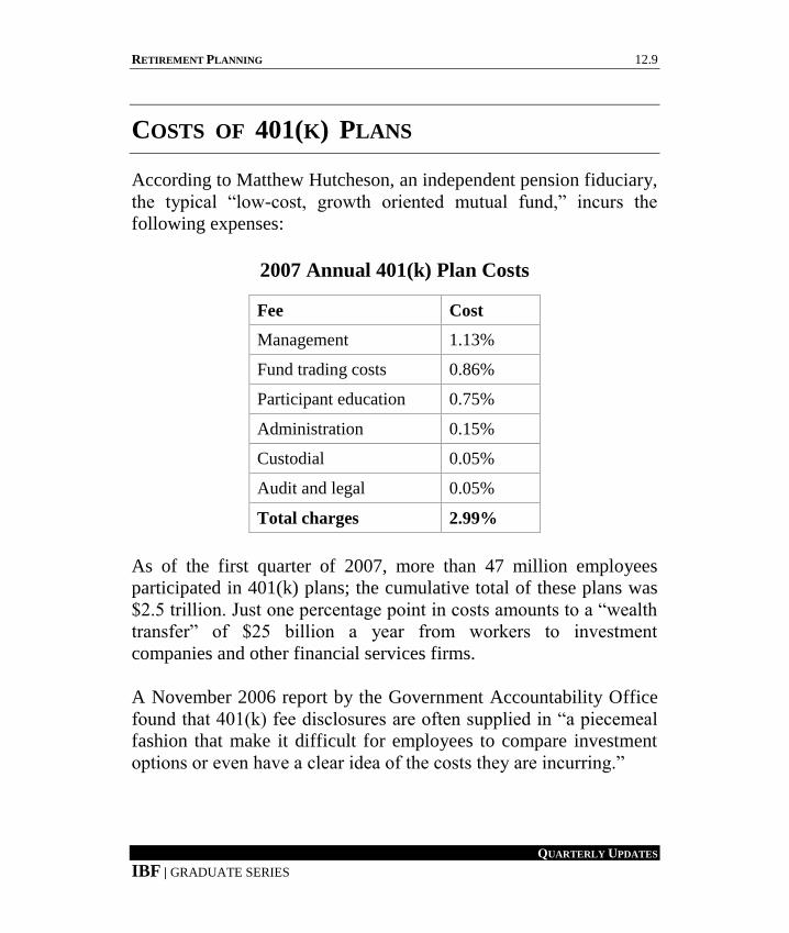
RETIREMENT PLANNING 12.9
QUARTERLY UPDATES
IBF | GRADUATE SERIES
COSTS OF 401(K) PLANS
According to Matthew Hutcheson, an independent pension fiduciary,
the typical “low-cost, growth oriented mutual fund,” incurs the
following expenses:
2007 Annual 401(k) Plan Costs
Fee Cost
Management 1.13%
Fund trading costs 0.86%
Participant education 0.75%
Administration 0.15%
Custodial 0.05%
Audit and legal 0.05%
Total charges 2.99%
As of the first quarter of 2007, more than 47 million employees
participated in 401(k) plans; the cumulative total of these plans was
$2.5 trillion. Just one percentage point in costs amounts to a “wealth
transfer” of $25 billion a year from workers to investment
companies and other financial services firms.
A November 2006 report by the Government Accountability Office
found that 401(k) fee disclosures are often supplied in “a piecemeal
fashion that make it difficult for employees to compare investment
options or even have a clear idea of the costs they are incurring.”

12.10 RETIREMENT PLANNING
QUARTERLY UPDATES
IBF | GRADUATE SERIES
RETIREMENT STATISTICS
According to a 2005 study by the Urban Institute in Washington,
people age 75 and older typically spend 10% less per person than
those age 65 to 74. It appears that this drop in spending may not be
“voluntary.”
The U.S. Census Bureau reports that seniors have an average
household net worth of $100,000, versus $120,000 for those age
70 to 74 and $114,000 for those 65 to 69 (note: all of these figures
include home equity). If you strip out home equity, households
headed by someone age 75 and older have a typical net worth of
just $19,000. As a side note, annual inflation for seniors over the
past 20 years has been 3.2% versus 3.0% for the general public.
MAXIMUM SOCIAL SECURITY BENEFIT
According to the Social Security Administration, an individual
retiring in 2007 who is eligible for the maximum Social Security
retirement benefit will receive $2,116 per month, or $25,392 for the
first year. According to Kiplinger, 58% of Americans believe they
will need to accumulate at least $2 million in savings in order to
enjoy a comfortable retirement.

RETIREMENT PLANNING 12.11
QUARTERLY UPDATES
IBF | GRADUATE SERIES
PEOPLE WORKING LONGER
In 2006, over 26% of California residents between the ages of 65
and 69 were still working (vs. 20% in 1995). Roughly 40% of this
age group that is still working is doing so because they feel that they
have not saved enough money for retirement.
The median balance in a 401(k) plan or IRA for the head of
household between the ages of 55 and 64 in California is about
$60,000; this translates into an inflation-indexed annuity of just $250
per month. If people were to retire at age 67 instead of 65, the
percentage of retirees “at risk” (not having enough money to
maintain their lifestyles during retirement) drops from 43% to 32%.
If workers could save just 3% more of their earnings each year, the
“at risk” numbers would drop another 11%.
INFLATION MEASUREMENTS
The U.S. consumer price index (CPI) has increased by an annualized
rate of just under 3% over the last 25 years (1982-2006). Yet, a
major risk during retirement is the retiree’s age-specific personal
inflation rate (see second table).
The first table below shows the long-term impact of inflation at
various rates, ranging from 0-4% annually. For example, if inflation
were to continue to average 3% a year, $1,000 would have the
purchasing power of $744 in 10 years.

12.12 RETIREMENT PLANNING
QUARTERLY UPDATES
IBF | GRADUATE SERIES
Purchasing Power of $1,000 at Different Rates of Inflation
Year 0% 1% 2% 3% 4%
1 $1,000 $990 $980 $971 $962
5 $1,000 $951 $906 $863 $822
10 $1,000 $905 $820 $744 $676
15 $1,000 $861 $743 $642 $555
20 $1,000 $820 $673 $554 $456
25 $1,000 $780 $610 $478 $375
30 $1,000 $742 $552 $412 $308
35 $1,000 $706 $500 $355 $253
The next table is something most advisors have never seen, the CPI-
E (the inflation rate that is unique to Americans age 62 and
older), which is compiled by the U.S. Department of Labor through
its Bureau of Labor Statistics (BLS).
Like the traditional CPI-W (“W” is for “wage earners”), each month
the CPI-E measures price changes for hundreds of categories and
items. Category weighting is based on average spending habits for
the group.
The CPI-W reflects the spending habits of just under a third of
the U.S. population. For example, working Americans spend four
times as much on food and beverages as on apparel (0.16 vs. 0.04);
they also spend eight times more on housing than they do on
recreation (0.41 vs. 0.05).

RETIREMENT PLANNING 12.13
QUARTERLY UPDATES
IBF | GRADUATE SERIES
The table below shows the components that comprise the CPI-W
index and CPI-E index plus their various component weightings; the
“% of whole” column for each index, excluding “All items,” adds up
to 1.00. The higher the component weighting, the more a price
change for the category will affect the overall inflation rate. For
example, notice how “Education & Communication” for the elderly
represents just 50% of what it does for workers.
CPI-W (workers) and CPI-E (elderly) Inflation Rates
Component
% of
whole
10-yr.
Inflation
% of
whole
10-yr
Inflation
All items 1.00 26.5% 1.00 29.7%
Apparel 0.04 -8.3% 0.03 -8.9%
Education & Communication 0.06 18.2% 0.03 4.5%
Food & Beverages 0.16 25.9% 0.13 25.4%
Housing 0.41 32.8% 0.48 34.0%
Medical Care 0.05 47.8% 0.11 47.8%
Recreation 0.05 9.8% 0.05 18.3%
Transportation 0.20 20.4% 0.15 21.9%
Other Goods & Services 0.04 56% 0.04 45.5%
From 1982 to the end of 2006, the inflation rate for U.S. workers
averaged just under 3% a year, versus 3.3% for the elderly. In fact,
for each and every year over the past quarter of a century, CPI-E
increases have been greater than CPI-W increases.

12.14 RETIREMENT PLANNING
QUARTERLY UPDATES
IBF | GRADUATE SERIES
The discussion as to how to personalize a client’s CPI rate becomes
more interesting when gender and geography are factored in. For
example, over the past 10 year, the rate of inflation has averaged
2.3% in Atlanta but 3.5% in San Diego. A report by Merrill Lynch
shows that the recent inflation rate for women has been about 3.6%
but just 0.2% for males—because their spending habits are different.
Client Customization A way to differentiate yourself from your peers is to sit down with
your older clients and comprise a CPI for each, based on how that
person (or couple) actually spends money. For example, suppose
you have a client that spends all of her money on just two things,
housing and medical care (for this simple example, pretend the client
does not travel or eat, etc.). In such a case, her cumulative rate of
inflation over the past 10 years would have been 41% [(34% + 48%)
/ 2] and her annualized rate would have been 3.5%.
Perhaps a more meaningful adjustment would be for you to match
(or hedge) your clients’ expenditures with their equity holdings. For
example, if a client spent 20% of their income on drugs and other
medications, roughly 20% of their equity exposure could be in the
pharmaceutical and healthcare sectors.
RETIREMENT PLANNING 12.15
QUARTERLY UPDATES
IBF | GRADUATE SERIES
LONG-TERM CARE PARTNERSHIP
The idea behind Partnership for Long-Term Care, an insurance
program used in five states (California, Connecticut, Idaho, Indiana,
and New York) is that if you buy a long-term care policy that is
approved by the state, you can apply for Medicaid to help cover any
additional costs. Moreover, you can keep assets equal in value to the
insurance benefits received. This means assets do not have to be
“spent down” before a patient qualifies for Medicaid.
For example, if you have a client that buys a policy whose
cumulative benefit is $100,000 (e.g., $100 a day for 1,000 days), he
or she can keep $100,000 in personal assets and still qualify for
Medicaid. For the vast majority of your clients, three years of long-
term care insurance coverage should be more than enough.
According to a 2005 actuarial survey of 1.6 million active policies,
only eight in 100 claimants with a three-year benefit period
exhausted their coverage.
For 2006, the average daily cost for a shared nursing home room
nationwide was $183 ($66,795 a year) according to MetLife Inc.
research. However, the average in New York City was $333 per day
(or $121,545 a year). The national average hourly rate for a home
health care aide is $19; the highest regional figure was $29 an hour
in Rochester Minnesota.

12.16 RETIREMENT PLANNING
QUARTERLY UPDATES
IBF | GRADUATE SERIES
When considering long-term care coverage, focus on the following:
1. Opt for an inflation protection rider (annual benefit
compounds at 5%).
2. Lifetime benefits can cost up to 40% more than three years
of benefits.
3. Find out average costs for care where the client lives.
4. Determine the financial strength of the carrier
(www.ambest.com).
5. If the client is in good health, use companies that have
extensive tests.
6. If the client is in poor health, one rejection is not universal.
At least 25 more states are expected to pass the Partnership for
Long-Term Care during the next few years. The following web sites
can help you figure out the cost of long-term care insurance where
your clients live:
1. www.longtermcare.gov: Under “Paying for Long-Term
Care,” go to “Cost of Care.”
2. www.metlife.com/maturemarketinstitute: Click on “Studies,”
then go to “2006 MetLife Market Survey of Nursing Home
and Home Care Costs.”
3. www.longtermcare.genworth.com: go to “What is the Cost of
Long-Term Care?”
4. www.notaburden.com (MassMutual’s web site for financial
professionals): Under the “For Producers” link, look under
the “Cost by State Calculator.”
RETIREMENT PLANNING 12.17
QUARTERLY UPDATES
IBF | GRADUATE SERIES
DISCLOSURE FOR ORGAN DONORS
Before the end of the third quarter of 2007, prospective organ donors
will gain greater information. Specifically, transplant centers will be
required to detail the risks of donor surgery plus they must provide
independent patient advocates. The quality of transplants will be
compared against Medicare and Medicaid standards. All transplant
centers must be recertified every three years. Those that fare worse
than would be statistically expected risk losing their Medicare
funding.
There are 300 transplant centers in the U.S.; the number of living
donors in 2006 doubled to nearly 7,000. The vast majority are liver
donors. Under the new regulations, prospective living donors are
given statistics on how recipients and donors fare nationally and at
their hospital.
Potential donors must also be told about medical and psychological
risks, the surgical procedure and post-operative treatment as well as
alternate treatments. Additionally, the donor must be informed that
his or her health insurance may not cover future health problems
related to the donation and that the donor may have difficulty
obtaining health, disability, or life insurance in the future.

12.18 RETIREMENT PLANNING
QUARTERLY UPDATES
IBF | GRADUATE SERIES
FULLY FUNDED PENSION PLANS
For the first time since 2000, the assets of defined benefit pension
plans offered by Fortune 100 companies exceeded plan liabilities (as
of the middle of 2007), according to the consulting firm Towers
Perrin.
NEW MEDICAID RULES
New Medicaid rules eliminate the “resource first” option. All
states are now required to use the “income first” method, which
takes into account the patient spouse’s income as well as the
income of the patient. Some elder advocates believe these new
rules will increase the likelihood of divorce being used.
The new rules also extend the “look-back period” for gifts from
three to five years in most instances. The penalty period is now
computed differently. The clock starts on the penalty period from
the date the patient is eligible to receive Medicaid, instead of
from the date of the gift transfer.
For example, if Ted (the patient) made a $20,000 gift four years ago,
then went to a nursing home, spent down his life savings over two
years, and then applied for Medicaid, he would still be subject to an
additional four-month waiting period ($20,000 divided by the
monthly cost of a nursing home, $5,000 in this example). If the gift
were large enough, the alternative would be to wait for an additional
year, so that a total of five years had lapsed since the time of the gift
and the commencement of nursing home care.

RETIREMENT PLANNING 12.19
QUARTERLY UPDATES
IBF | GRADUATE SERIES
Under the new rules, an annuity is not counted an asset if the state is
named as a “remainder beneficiary” (so the state can later be
reimbursed). Annuities still remain an attractive strategy. The
annuity contract could remain in deferral mode until the Medicaid
application was submitted. At such time, the contract could then be
irrevocably annuitized. The tricky part is that actuarial life
expectancy tables are not those of the Internal Revenue Code or
Social Security.
Additionally, loans and mortgages must have a repayment schedule
that is actuarially sound; payments must be in equal amounts during
the term of the loan. There can be no deferral of payments and no
balloon payments. Upon death (of the Medicaid recipient), the loan
balance cannot be cancelled.
In the past, Medicaid planning relied on the fact that a home, no
matter how valuable, was considered an exempt asset. Under the
new rules, states must consider an applicant’s home equity in
excess of $500,000. States are permitted to raise that threshold to
$750,000. The result is that reverse mortgages may become more
popular if a large portion of the applicant’s net worth is in his or her
personal residence.


QUARTERLY
UPDATES
TAXES


TAXES 13.1
QUARTERLY UPDATES
IBF | GRADUATE SERIES
13.2007 TAX BREAKS
For 2007, the maximum 401(k) contribution increases to $15,500
($20,500 if the participant is age 50+). The maximum traditional and
Roth IRA annual contributions stay at $4,000 ($5,000 if age 50+). A
child or any other non-spouse who inherits a qualified retirement
account can now transfer it directly into an IRA. Such a transfer
allows the heir to stretch out distributions over numerous years.
Taxpayer’s age 70 1/2 or older can transfer as much as $100,000
directly from an IRA to a qualified charity. This transfer, also
allowed for 2006, is set to expire at the end of 2007.
The maximum federal estate tax rate is 45% for estates of people
who die in 2007. The basic federal estate tax exclusion remains at $2
million in 2007 and 2008; the exclusion is scheduled to rise to $3.5
million 2009, become unlimited in 2010, and then drop back down
to $1 million for estates created in 2011.
Taxpayers who use their car for business have a choice of deducting
their actual costs or using the IRS’s standard mileage rate; the 2007
rate is 48.5¢ (20¢ per mile for medical and moving purposes).

13.2 TAXES
QUARTERLY UPDATES
IBF | GRADUATE SERIES
TAX DOCUMENTS
The type of account(s) and activity determines the tax forms sent.
Mutual Fund Tax Information and Expected Mailing Date
Document Sent To Information Contained
Fund year-end
statement
[early January]
All fund accounts that
remain open after
September 30th
All account activity:
Cost basis of all shares purchased, reinvested,
year-end values, & RMD notice to IRA owners
who will be 70 1/2 that year
Form 1099-DIV
[late January]
Most non-retirement &
non-educational accounts
Ordinary & qualified dividends, capital gains
distributions, federal taxes withheld, &
foreign taxes paid
Form 1099-B
[late January]
Most non-retirement &
non-educational accounts
Date of each sale, number of shares sold,
share price, dollar amount of each transaction,
plus average cost basis & gain or loss
information for most accounts
Form 1099-INT
[late January]
Most non-retirement &
non-educational accounts
invested in muni bonds
Federally tax-exempt income dividends from
muni bond funds & any private- activity bond
interest used to compute AMT
Form 1099-R
[late January]
IRAs & other retirement
accounts
Distributions from Roth, traditional, SEP,
& simple IRAs, plus distributions from
most retirement plans
Form 1099-Q
[late January]
Educational & Coverdell
accounts
Distributions from educational accounts
Form 5498
[late May]
IRAs All contributions, transfers, & rollovers to
traditional & Roth IRAs plus SEP IRAs;
year-end market values of IRA accounts
Form 5498-ESA
[late April]
Coverdell accounts Coverdell contributions & transfers
(sent to beneficiary, not contributor)

TAXES 13.3
QUARTERLY UPDATES
IBF | GRADUATE SERIES
FREE TAX PREPARATION AND FILING
In 2006, the U.S. Government Accountability Office estimated that
38% of taxpayers with securities transactions during the 2001 tax
year misreported their capital gains or losses. TurboTax has a tool
called BasicPro that taps into a database to help advisors and
clients determine cost basis. Another service, AccuBasis, offered
by Depository Trust & Clearing and NetWorth Services, also
provides similar information.
If you have clients with an AGI of $52,000 or less, they can go to
irs.gov and click “2007 Free File.” From there your client will be
linked to companies that will let them use their software and
then file the return, all for free. Some companies, including Intuit,
the makers of TurboTax, offer basic versions of their software on
their own sites to anyone at any income level.
TAX FACTS
The 16th
Amendment created the federal income tax in 1913. In its
first year, it taxed incomes of more than $3,000 at 1% and incomes
of more than $20,000 ($400,000 in today’s dollars) at rates from 2-
7%. Form 1040, the main tax-filing application, got its name because
it was the 1,040th
form issued by the Bureau of Internal Revenue, the
predecessor to the IRS.

13.4 TAXES
QUARTERLY UPDATES
IBF | GRADUATE SERIES
The first electronic transmission of a tax return to the IRS occurred
in 1986; for the 2006 calendar year, more than 73 million people
filed electronic returns. The IRS estimates the overall compliance
rate at 84%. In 2001, taxpayers paid, on average, a “surtax” of more
than $2,000 each to subsidize noncompliance by others. In 2000,
each $100 collected by the IRS cost 39¢ to collect.
In the beginning (1914), the original 1040 form was so small the
New York Times printed it on their front page. There were just four
instructions; now there are 4,000. By 1918, the government needed
money to fight World War I and the top rate was increased to 70%.
In 1914, total income tax collections were $10 billion, in today’s
dollars. The original IRS enforcement office had 4,000 employees.
Today, roughly $1 trillion is collected each year and the IRS has
100,000 tax agents. The New York Times wrote an editorial in 1909,
warning against the possibility of an income tax, “When men get in
the habit of helping themselves to the property of others, they cannot
be easily cured of it.”
During the early years of the income tax, only about 1/2% of
Americans (360,000) had to fill out a tax form. Today, 135 million
do so; nearly every U.S. worker. As a side note, when the AMT was
passed in 1969, it was originally designed to force just 155 wealthy
individuals to pay taxes. For 2006, six million were subject to the
AMT. If Congress does not intervene, 26 million will be subject to
this tax in 2007.

TAXES 13.5
QUARTERLY UPDATES
IBF | GRADUATE SERIES
For 2007, there are over 66,000 pages of tax laws to contend with,
along with 526 separate forms. It is estimated that 1.2 million people
are employed as tax accountants, lawyers, and tax preparers.
American workers and businesses devote 6.4 billion hours a year, or
roughly 45 hours per return. For example, there are now 16 different
tax breaks for college education. Two-thirds of the adult population
cannot figure out basic IRS regulations or tax laws concerning the
sale of a home. According to the IRS, the number of federal estate
tax returns (Form 706) for the 2007 calendar year is expected to be
30,400 (versus 90,000 in 1997).
APPEAL TO CHILDREN
A number of mutual fund families now have programs and
specialized products designed to appeal to investors age 20 and
younger. American Century Investments offers “My [Whatever]
Plan,” an online financial coach that goes over a savings strategy
based on a specific goal, such as a wedding, buying a home, or
retirement. Investors must commit $500 upfront and $100 a month
thereafter.
Charles Schwab has a four-step IRA program that requires a $2,000
minimum investment; the materials show that by cutting out just two
nights per month of partying, the young adult can end up with quite
a bit of money. The Monetta Young Investor fund has a web site
with a financial literacy area and a stock-picking game where
children can win prizes; account holders earn 5% of their annual
account balance in tuition credits.

13.6 TAXES
QUARTERLY UPDATES
IBF | GRADUATE SERIES
FEDERAL RESERVE COMIC BOOKS
For the past half century, the New York Federal Reserve has been
publishing comic books whose target audience is high school
students (over 850,000 copies distributed in 2006). The Fed comic
book most in demand is “Once Upon a Dime.” The storyline is about
how money came to be on a mythical tropical island called Mazuma.
Advisors who have clients who are looking to educate their children
and grandchildren can visit the newyorkfed.org web site and click on
“publications catalog” to order the comics at no charge.
YOUNG INVESTORS
The University of Minnesota has found that children as young as age
five can develop spending and saving habits. The Investment
Company Institute (ICI), the trade and lobbying group of mutual
funds, lists child-friendly web sites (www.ici.org/funds/inv/
resourcesyoung.html.).