1

Investment Analysis 1

BEAM011

Lecture 5

Valuation Models

Dr Jon Tucker

Xfi Centre for Finance and Investment

University of Exeter

Lecture Objectives

1. To introduce four basic valuation models:

� Dividend Discount Model

� Price Multiples Model

� Free Cash Flow Model

� Residual Income Model

2. A reminder on the cost of capital

2

The Dividend Discount ModelProbably one of the most simple and widely used models of equity valuation is

the Dividend Discount Model (DDM). In this model, the firm is valued in relation

to the cash flows which it generates generally, though focuses on distributed

earnings of the firm, that is, dividends. After all, until the investor sells his or her

equity investment in a firm, their cash returns are solely in the form of dividends.

One important question here is, “what about retained earnings – does the

dividend discount model ignore these?” The answer is clearly “no”. Indeed,

earnings reinvested in the firm rather than being paid out will provide the basis

for enhanced future dividends. As the growth path of dividends is fairly smooth

for most firms, the DDM valuation is easier to produce and is considered a good

measure of long-run intrinsic value.

Dividend discount models are of greatest use when:

• The company concerned actually pays a dividend

• There is a clear company policy linking dividends to underlying earnings

The Basis of the DDMThe basis of the DDM, then, is that the price to be paid for an equity in the market should reflect the future stream of dividend payments accruing to the equity investor. Lets start with the simplest case of an investor who is considering buying a share and holding it for one year before selling it again. What price should they pay for that share?

)r1(

PD

)r1(

P

)r1(

DV 1111

0 +

+=

++

+=

Here:

V0 = value of the share today (at t=0)

P1 = expected price that share could be sold for at time t+1

D1 = expected dividend for that share during the year

r = required rate or return on the share

Equity value

(Price today) = Price next year +

Dividend during

year

3

A DDM ExampleLets look at an example of this simplest of DDMs. Company DEF is

expected to pay a dividend of £1.00 next year and is expected to sell for

£15.00 at the end of that period. The required rate of return for equity

holders of DEF is 8 per cent. What value should be placed on the share

today?

)r1(

PD

)r1(

P

)r1(

DV 1111

0 +

+=

++

+=

81.14£)08.1(

00.1500.1

)r1(

PDV 11

0 =+

=+

+=

The fact that the price is expected to decrease reflects the fact that it is

not expected to pay at least the expected rate of return on an equity of

that class and cover the time value of money.

The Gordon Growth ModelHowever, very few shareholders buy a share with the intention of selling it in one year’s time. Many investors and funds have the intention of buying a share to hold for a much longer time period, often as a key component of a retirement investment. How we deal with this fact is that we assume that we can make forecasts of dividends over some finite time horizon and then we estimate a terminal value thereafter.

A model known as the Gordon Growth Model helps us with the problem of longer-term shareholdings. If we can observe the current dividend payment to shareholders, estimate the expected growth rate of those dividends into the future, and observe the required rate of return on that type of equity, then we can calculate the firm’s equity value:

gr

D

gr

)g1(DV 10

0 −=

−

+=

Note that an interesting shortcoming of this model is that the cost of equity

capital, r, must always be greater than g, the growth rate of dividends.

Otherwise, if r=g, the value of the equity is infinite or if r<g, the value of the

equity is negative. Clearly, neither of these valuation outcomes is very

useful!

4

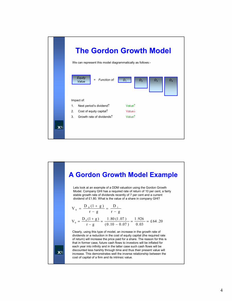
The Gordon Growth Model

Equity

Value= Function of: D1 D2 D3 D4

Impact of:

1. Next period’s dividend↑ Value↑

2. Cost of equity capital↑ Value↓

3. Growth rate of dividends↑ Value↑

We can represent this model diagrammatically as follows:-

A Gordon Growth Model Example

Lets look at an example of a DDM valuation using the Gordon Growth

Model. Company GHI has a required rate of return of 10 per cent, a fairly

stable growth rate of dividends recently of 7 per cent and a current

dividend of £1.80. What is the value of a share in company GHI?

gr

D

gr

)g1(DV 10

0 −=

−

+=

20.64£03.0

926.1

)07.010.0(

)07.1(80.1

gr

)g1(DV 0

0 ==−

=−

+=

Clearly, using this type of model, an increase in the growth rate of

dividends or a reduction in the cost of equity capital (the required rate

of return) will increase the price paid for a share. The reason for this is

that in former case, future cash flows to investors will be inflated for

each year into infinity and in the latter case such cash flows will be

discounted less harshly through time and thus their present value will

increase. This demonstrates well the inverse relationship between the

cost of capital of a firm and its intrinsic value.

5

Another extension to the DDM is needed to help us with real world valuation

problems. How do we deal with a firm which is not expected to have a stable or

constant growth rate into the indefinite future? Growth often falls into three

stages for a company:

1. Growth – Often during a growth phase, companies pay low dividends or even

miss them.

2. Transition – Once the growth phase has slowed and a firm’s markets are

maturing, free cash flows then become positive and the firm increases its

dividends.

3. Maturity – Here, once the firm’s markets have matured and returns on equity

approximate their costs, the path of dividends stabilises to a sustainable

pattern. The Gordon Growth Model can be very useful for valuing firms in this

phase.

The Multiple Growth Rate Model

Dividends

Per share

Growth stage

Growth

Transition

Maturity

A Multiple Growth Rate Example

Arriving at an equity value for firms which will experience multiple growth rates

into the future is perhaps a more difficult task, though the principles are simple.

Lets look at an example firm. We expect the dividends of firm JKL to grow at 8

per cent for the next two years, 14 per cent for the following 4 years, and to

settle at 10 per cent thereafter. The required rate of return for the company is

11 per cent. The company’s current dividend is £0.75 per year. What is the

value of an equity share in the company JKL?

Three periods of growth for JKL:

Dividend

Growth Rate

Year

1 2 3 4 5 6 7 8 …

5%

10%

15%

6

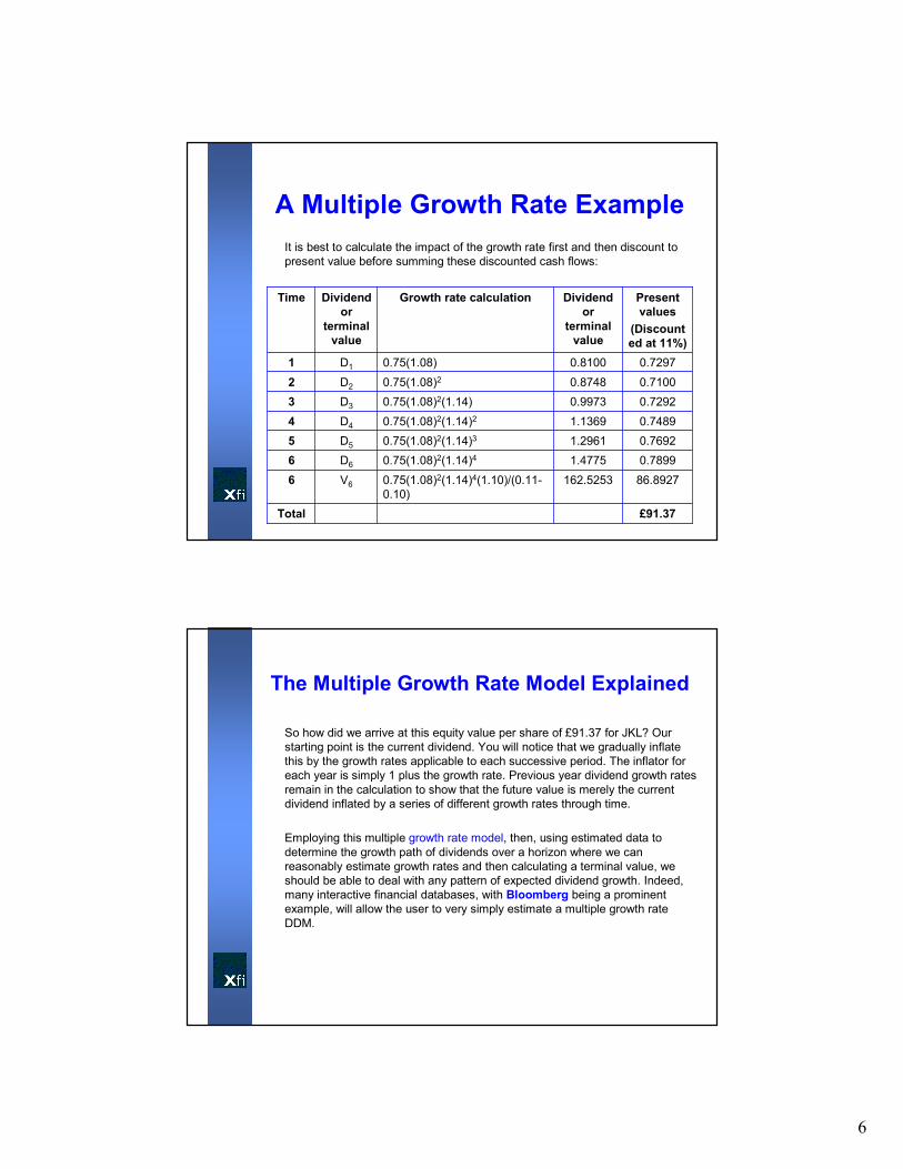
A Multiple Growth Rate Example

It is best to calculate the impact of the growth rate first and then discount to

present value before summing these discounted cash flows:

£91.37Total

86.8927162.52530.75(1.08)2(1.14)4(1.10)/(0.11-

0.10)

V66

0.78991.47750.75(1.08)2(1.14)4D66

0.76921.29610.75(1.08)2(1.14)3D55

0.74891.13690.75(1.08)2(1.14)2D44

0.72920.99730.75(1.08)2(1.14)D33

0.71000.87480.75(1.08)2D22

0.72970.81000.75(1.08)D11

Present

values

(Discount

ed at 11%)

Dividend

or

terminal

value

Growth rate calculationDividend

or

terminal

value

Time

So how did we arrive at this equity value per share of £91.37 for JKL? Our

starting point is the current dividend. You will notice that we gradually inflate

this by the growth rates applicable to each successive period. The inflator for

each year is simply 1 plus the growth rate. Previous year dividend growth rates

remain in the calculation to show that the future value is merely the current

dividend inflated by a series of different growth rates through time.

Employing this multiple growth rate model, then, using estimated data to

determine the growth path of dividends over a horizon where we can

reasonably estimate growth rates and then calculating a terminal value, we

should be able to deal with any pattern of expected dividend growth. Indeed,

many interactive financial databases, with Bloomberg being a prominent

example, will allow the user to very simply estimate a multiple growth rate

DDM.

The Multiple Growth Rate Model Explained

7

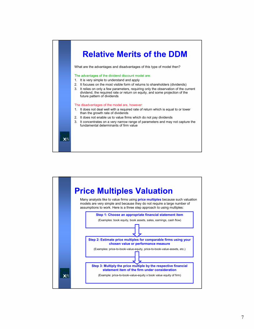
What are the advantages and disadvantages of this type of model then?

The advantages of the dividend discount model are:

1. It is very simple to understand and apply

2. It focuses on the most visible form of returns to shareholders (dividends)

3. It relies on only a few parameters, requiring only the observation of the current dividend, the required rate or return on equity, and some projection of the future pattern of dividends

The disadvantages of the model are, however:

1. It does not deal well with a required rate of return which is equal to or lower than the growth rate of dividends

2. It does not enable us to value firms which do not pay dividends

3. It concentrates on a very narrow range of parameters and may not capture the fundamental determinants of firm value

Relative Merits of the DDM

Step 1: Choose an appropriate financial statement item

(Examples: book equity, book assets, sales, earnings, cash flow)

Step 2: Estimate price multiples for comparable firms using your

chosen value or performance measure

(Examples: price-to-book-value-equity, price-to-book-value-assets, etc.)

Step 3: Multiply the price multiple by the respective financial

statement item of the firm under consideration

(Example: price-to-book-value-equity x book value equity of firm)

Many analysts like to value firms using price multiples because such valuation

models are very simple and because they do not require a large number of

assumptions to work. Here is a three step approach to using multiples:

Price Multiples Valuation

8

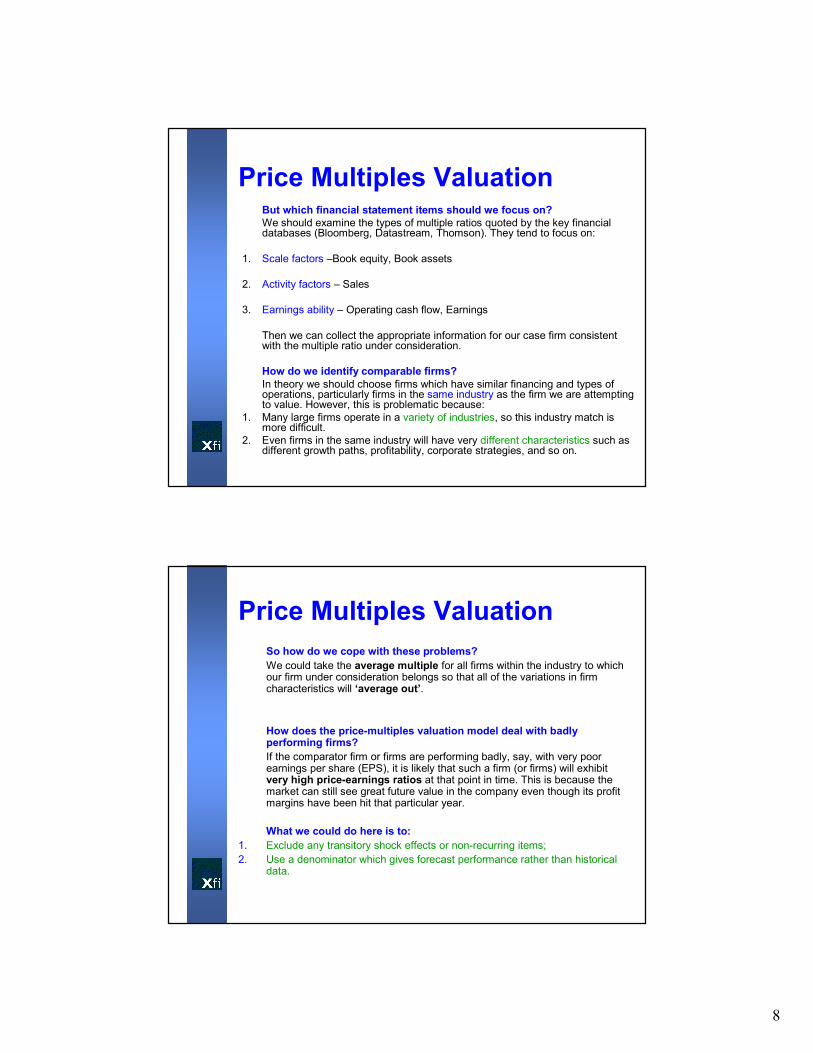
But which financial statement items should we focus on?

We should examine the types of multiple ratios quoted by the key financial databases (Bloomberg, Datastream, Thomson). They tend to focus on:

1. Scale factors –Book equity, Book assets

2. Activity factors – Sales

3. Earnings ability – Operating cash flow, Earnings

Then we can collect the appropriate information for our case firm consistent with the multiple ratio under consideration.

How do we identify comparable firms?

In theory we should choose firms which have similar financing and types of operations, particularly firms in the same industry as the firm we are attempting to value. However, this is problematic because:

1. Many large firms operate in a variety of industries, so this industry match is more difficult.

2. Even firms in the same industry will have very different characteristics such as different growth paths, profitability, corporate strategies, and so on.

Price Multiples Valuation

So how do we cope with these problems?

We could take the average multiple for all firms within the industry to which our firm under consideration belongs so that all of the variations in firm characteristics will ‘average out’.

How does the price-multiples valuation model deal with badly performing firms?

If the comparator firm or firms are performing badly, say, with very poor earnings per share (EPS), it is likely that such a firm (or firms) will exhibit very high price-earnings ratios at that point in time. This is because the market can still see great future value in the company even though its profit margins have been hit that particular year.

What we could do here is to:

1. Exclude any transitory shock effects or non-recurring items;

2. Use a denominator which gives forecast performance rather than historical data.

Price Multiples Valuation

9

The price-earnings multiple model which we examined earlier can be refinedto take into account changes in:

1. Market expectations (through price-earnings PE growth)

2. Earnings growth (measured by earnings per share EPS growth)

In so doing, we can project share prices to particular points in the future.

Forecast price = Current price x PE growth x Earnings growth

For example, an Analyst forecasts growth of 28% in earnings per share over the next year for a company with a current share price of £15.00. He looks back on the company’s history and finds that over the last 5 years the company’s sector P/E averaged 16 but rose steadily to 18 at present, approximately the same as the company. He expects the sector P/E to continue rising and forecasts a future (next year) P/E for the company of 20

Together with his earnings growth forecast this implies a forecast price of:

Forecast price = Current price x PE growth x Earnings growth

15 x (20/18) x 1.28 = £21.33

Price Multiples Valuation

Price Multiples ModelsComparable Companies Approach

As we have already discussed, the basis for multiples valuation is that we

judge what to pay for an equity share by looking to see what investor cash will

buy for similar firms in terms of:

• Scale (P/B)

• Activity (P/S)

• Earnings ability (P/E, P/CF)

Cornell’s Comparable Companies Approach uses a number of different

multiples simultaneously to value a company.

The basis for the technique is that similar companies should sell for similar

prices. We should therefore calculate multiples for a group of similar

companies. Lets illustrate with an example.

10

Price Multiples Models

18221715Market / Net income

= P/E ratio

1.61.51.32.0Market / Book

1.00.71.31.0Market / Sales

MeanCompany CCompany

B

Company

A

Ratio

We wish to value company MNO in relation to its main industry

competitors using the Comparable Companies Approach. How do we

go about this?

1. Find comparable companies – in this case companies A, B and C

2. Calculate a number of multiples ratios – in this case market to sales,

book and earnings

3. Calculate the mean of these ratios – across companies A, B and C

4. Apply these mean multiples to absolute data for company MNO –

multiply each mean ratio by the respective financial statement figure for

MNO

Price Multiples ModelsNext, we can apply these mean ratios to the respective figures drawn from

the financial statements for company MNO:

£1,120,000Mean

1,080,0001860,000Net income

1,280,0001.6800,000Book value equity

1,000,0001.01,000,000Sales

Suggested value of

equity

£

Mean market ratioActual Financial

Statement Data

For Company MNO

£

Financial Statement

Item

Thus, we are able to generate a suggested or indicated value for the

company MNO of £1,120,000. This technique draws upon what we have

already learned about price multiples and is very simple. More importantly, it

can also be used to value a firm which is not quoted on a stock exchange

and thus is particularly useful in arriving at a reasonable price for a company

which is considering listing for the first time.

11

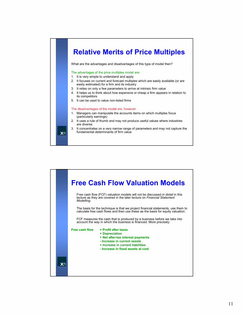
What are the advantages and disadvantages of this type of model then?

The advantages of the price multiples model are:

1. It is very simple to understand and apply

2. It focuses on current and forecast multiples which are easily available (or are easily estimated) for a firm and its industry

3. It relies on only a few parameters to arrive at intrinsic firm value

4. It helps us to think about how expensive or cheap a firm appears in relation to its competitors

5. It can be used to value non-listed firms

The disadvantages of the model are, however:

1. Managers can manipulate the accounts items on which multiples focus (particularly earnings)

2. It uses a rule of thumb and may not produce useful values where industries are diverse

3. It concentrates on a very narrow range of parameters and may not capture the fundamental determinants of firm value

Relative Merits of Price Multiples

Free Cash Flow Valuation Models

Free cash flow (FCF) valuation models will not be discussed in detail in this lecture as they are covered in the later lecture on Financial Statement Modelling.

The basis for the technique is that we project financial statements, use them to calculate free cash flows and then use these as the basis for equity valuation.

FCF measures the cash that is produced by a business before we take into account the way in which the business is financed. More precisely:

Free cash flow = Profit after taxes

+ Depreciation

+ Net after-tax interest payments

- Increase in current assets

+ Increase in current liabilities

- Increase in fixed assets at cost

12

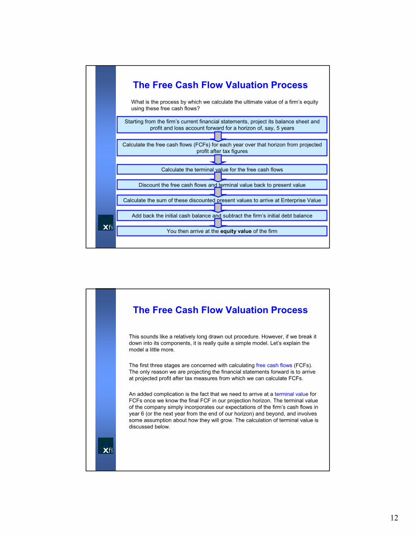
What is the process by which we calculate the ultimate value of a firm’s equity

using these free cash flows?

The Free Cash Flow Valuation Process

Starting from the firm’s current financial statements, project its balance sheet and

profit and loss account forward for a horizon of, say, 5 years

Calculate the free cash flows (FCFs) for each year over that horizon from projected

profit after tax figures

Calculate the terminal value for the free cash flows

Discount the free cash flows and terminal value back to present value

Calculate the sum of these discounted present values to arrive at Enterprise Value

Add back the initial cash balance and subtract the firm’s initial debt balance

You then arrive at the equity value of the firm

This sounds like a relatively long drawn out procedure. However, if we break it

down into its components, it is really quite a simple model. Let’s explain the

model a little more.

The first three stages are concerned with calculating free cash flows (FCFs).

The only reason we are projecting the financial statements forward is to arrive

at projected profit after tax measures from which we can calculate FCFs.

An added complication is the fact that we need to arrive at a terminal value for

FCFs once we know the final FCF in our projection horizon. The terminal value

of the company simply incorporates our expectations of the firm’s cash flows in

year 6 (or the next year from the end of our horizon) and beyond, and involves

some assumption about how they will grow. The calculation of terminal value is

discussed below.

The Free Cash Flow Valuation Process

13

The Calculation of Terminal and Enterprise Values

Terminal value is usually calculated in a very simple way:

growthWACC

)growth1(FCF5

−+×

In this expression:

FCF5 = Final year of projection horizon cash flow (e.g. year 5)

Growth = Expected growth rate of FCFs – we could simplify by assuming that

this is the growth rate of sales (for example) from year 6 into the

future

WACC = The firm’s weighted average cost of capital (the cost of its debt and

equity weighted by their proportion in the firm’s capital structure)

Once we have calculated the FCFs and terminal value we can then discount them back to their present value using the weighted average cost of capital (or WACC for short) and sum them to arrive at Enterprise Value. Enterprise Value (EV) is simply the sum of a firm’s capital structure components (the market value of debt plus equity).

Since EV is the sum of debt and equity, we must subtract the opening value of debt and add back the opening value of cash (and near-cash assets which are effectively ‘negative debt’) to arrive at the intrinsic value of equity.

A FCF Valuation ExampleSelected balance sheet and profit and loss items are given below for firm XYZ. The firm’s weighted average cost of capital is 14 per cent. Its initial cash and marketable securities (near-cash) balance is £80,000 and its initial debt balance is £400,000. The expected sales growth rate for year six and beyond is 12 per cent. All of the figures given below are in £ thousands. What is the value of the firm’s equity?

Selected financial statement items over the project horizon (years t+1 to t+5):

252117148

After-tax interest on cash and mkt.

securities

2222222222After-tax interest on debt

369319276238205Increase in fixed assets at cost

13121198Increase in current liabilities

2624211917Increase in current assets

227193163137115Depreciation

430386347311275Profit after tax

14

The FCF CalculationSo how do we get from these financial statement items to the FCF

valuation?

Our first task is to calculate the FCFs for XYZ for years t+1 to t+5 into the

future (over the forecast horizon):

272249229208190Free cash flow

(25)(21)(17)(14)(8)

Subtract after-tax interest on cash and mkt.

securities

2222222222Add back after-tax interest on debt

(369)(319)(276)(238)(205)

Subtract increase in fixed assets at

cost

13121198

Add back increase in current

liabilities

(26)(24)(21)(19)(17)Subtract increase in current assets

227193163137115Add back depreciation

430386347311275Profit after tax

Free cash flow calculation

Profit after tax

We start with profit after tax (PAT) as it is a measure which can most easily be

converted into a measure of free cash flow (FCF). Remember that we want a

measure of the cash available to shareholders regardless of the way in which

the firm is financed. Also, we understand that profit is not a very useful

measure of the cash ultimately available to shareholders as profit does not

equal cash due to accrual accounting (e.g. profit also accounts for

depreciation, investment in fixed and current assets, etc.)

Add back depreciation

We add back depreciation as it is an expense which does not involve a

movement of cash i.e. we do not physically spend cash when we run down the

value of fixed assets.

Subtract increase in current assets

We subtract any investment in current assets as this effectively reduces the

amount of cash available to shareholders as cash is ‘bound up’ in stock,

debtors, and so on.

Add back increase in current liabilities

We add back any increase in current liabilities as this is increasing the amount

of cash available to shareholders. Remember that current liabilities represent

suppliers and others who have allowed the firm credit terms which effectively

means that the amount of such liabilities is simply a form of ‘free cash’ or loan

available to the firm.

The FCF Calculation

15

Subtract increase in fixed assets at cost

As with our investment in current assets, we have to subtract from profit after

tax any investment in fixed assets as this represents cash ‘bound up’ in

productive capacity which is not then available to shareholders, unless they

liquidated the firm.

Add back after-tax interest on debt

We add back after-tax interest on debt (loans to the firm or bonds) as we want a

finance-free measure of cash available to shareholders. We could then

compare, in theory, the FCFs produced by similar firms, regardless of their

financial structure.

Subtract after-tax interest on cash and mkt. securities

If we have any interest-bearing bank deposits or any other short-term

investments which generate returns then we should also add them back to

profits as these increase the cash available to investors and are strictly

speaking a form of ‘negative debt’.

The FCF Calculation

Calculating the Terminal ValueOur next task is to calculate the terminal value for XYZ for year 6 into the

indefinite future:

growthWACC

)growth1(FCF5

−+×

Here, we simply substitute in figures that we now know. The last horizon year

FCF (FCF5) is £272,000, the growth rate we know to be 12 per cent, and the

WACC is 14 per cent. Thus the terminal value is:-

12.014.0

)12.01(000,272

−+×

Thus the terminal value of FCFs is computed to be £15,232,000. However,

we need to discount this and the horizon FCFs back to present value to

arrive at EV.

16

Calculating Enterprise ValueTo arrive at the present value, we simply have to discount all of the FCFs and the terminal value by the WACC:

55432 )14.1(

232,15

)14.1(

272

)14.1(

249

)14.1(

229

)14.1(

208

14.1

190EV +++++=

Thus the enterprise value for XYZ is calculated as:

166.67 + 160.05 + 154.57 + 147.43 + 141.27 + 7,911.02 =

£8,681,970

So the EV of XYZ is £8,681,970. We then need to add back cash and

marketable securities and subtract debt balances. Thus:

Enterprise value £8,681,010

Add initial cash 80,000

Subtract initial debt (400,000)

Equity value of XYZ £8,361,010

What are the advantages and disadvantages of this type of model then?

The advantages of the FCF model are:

1. It takes account of a very wide range of relevant accounting data

2. It can be used to calculate the intrinsic (market) value of either equity or debt

3. It encourages the analyst to examine the evolution of the financial statements

through the forecast horizon and to consider whether the projected growth

path of the firm is realistic

The disadvantages of the model are, however:

1. It is based on accounting data which can be subject to creative accounting

2. It requires a large investment of time to set up the underlying financial

statement model

3. It is very assumption sensitive, particularly with regard to future growth rates

Relative Merits of the FCF Valuation Model

17

Residual Income ModelsThe following relationship can be used to value a firm’s equity:

Residual income models were developed to correct a shortcoming of financial

statements – the fact that net income net income (profit) includes a charge for

the cost of a firm’s debt but not for the cost of its equity. The result of this is that

it is left to shareholders to decide whether:

Value

of equity

Book value

of equity

Present value of

expected future

abnormal earnings

= +

The firm’s

earningsare greater than The equity cost of

capital

If earnings are greater, then the firm is creating value, if they are less then the firm

may even be destroying value for shareholders.

Residual Income Models therefore deduct the cost of debt and equity from

earnings to arrive at a measure of income which takes into account the

opportunity costs of a firm’s shareholders.

The model is probably best explained with the aid of a simple example.

ABC Corporation, a small engineering company, has 50 per cent debt and 50

per cent equity in its capital structure. It has total assets of £5,000,000. Its cost

of debt capital is 8 per cent and its cost of equity capital is 14 per cent. The

earnings (earnings before interest and tax or EBIT) of the company are

£500,000 and it is subject to a tax rate of 30 per cent.

First of all, is ABC profitable from an accounting viewpoint?

A Residual Income Model Example

18

From an accounting viewpoint, lets calculate ABC’s net income:

£

EBIT 500,000

Less: Interest Expense (200,000)

-------------

Pre-tax Income 300,000

Less: Corporation Tax Expense (90,000)

-------------

Net Income £210,000

So, clearly ABC is profitable from an accounting viewpoint. However, are its

shareholders happy with this level of earnings? To answer this question, we

need to deduct a charge for the opportunity cost of shareholders’ funds (or,

put another way, an equity charge).

Calculating Net Income

This equity charge is simply the cost of equity capital in money terms:

Calculating Residual Income

Equity charge Equity funding

within capital

structure

Cost of equity

capital %= X

For ABC, the equity charge is therefore:

£2,500,000 X 14 per cent = £350,000

If we then deduct this from our Net Income figure of £210,000, we get a figure

for residual income:

£210,000 - £350,000 = (£140,000)

Thus our residual income figure is negative which implies that ABC, whilst

producing healthy accounting earnings, failed to cover the cost of equity capital

(failed to cover the opportunity costs of shareholders). ABC, in this sense is

destroying value as shareholders could get a far better return investing their

money elsewhere.

19

The Residual Income Model Concept

So far, all we have demonstrated is that residual income models are useful as

residual income is a concept which shareholders, fund managers and

companies themselves should be very much aware of.

Next, we should develop a general expression to be applied to a company to

actually calculate its equity value using this concept of residual income.

Value

of equity

Book value

of equity

Present value of

expected future

residual income

(or abnormal

earnings)

= +

The current book value of equity on the right hand side of the expression is a

straightforward figure to find from the financial statements. The present value of

expected future residual income can be expressed in one of two ways, as

follows.

Whether we wish to value a share in relation to residual income as calculated

above or in relation to earnings per share, we can employ the following

expression:

The Residual Income Model Expression

∑∑∞

=

−∞

= +

−+=

++=

1tt

1tt

1t0t

t00

)r1(

rBEB

)r1(

RIBV

0V = Value of share today (t=0)

0B = Book value of equity today

tB = Expected book value per-share at time t

r = Equity cost of capital

tE = Expected Earnings Per Share for period t

= Expected residual income per-share (Equals ) 1tt rBE −−tRI

20

This expression requires some explanation. If we can get data on earnings per

share (EPS) for a company, we can then deduct an equity charge per-share for

the period. This equity charge is defined as the required rate of return on equity

multiplied by the per-share opening book value of equity at the beginning of the

period in question.

A useful aspect of this second version of the residual income model is that we

can easily compare EPS at a particular time to the per-share equity charge to

determine whether residual income is positive or negative. The rule is:

If EPS > per-share cost of equity ⇒ Residual income per share is positive

If EPS < per-share cost of equity ⇒ Residual income per share is negative

Obviously, companies for which residual income is positive should sell for a

higher price than companies for which residual income is negative.

Residual Income and EPS

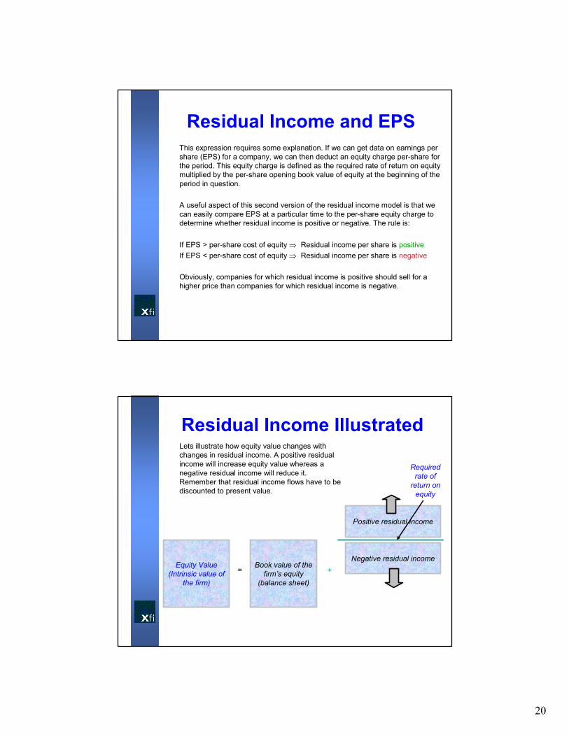
Lets illustrate how equity value changes with

changes in residual income. A positive residual

income will increase equity value whereas a

negative residual income will reduce it.

Remember that residual income flows have to be

discounted to present value.

Residual Income Illustrated

Equity Value

(Intrinsic value of

the firm)

Book value of the

firm’s equity

(balance sheet)

Positive residual income

Negative residual income

=

Required

rate of

return on

equity

+

21

Lets use the new expression which employs EPS to help us calculate equity

value for an example company.

The EPS of company PQR is expected to be £5.00, £6.00 and £8.00 for the

next three years. Investment analysts predict that the company is expected to

pay dividends of £2.50, £3.00 and £23.50 for those three years, the last

dividend being much larger as the company is expected to cease operations

after that year. In this respect the final dividend could be termed a liquidating

dividend. The current book value of PQR is £10.00 per share. Its required rate

of return on equity (its cost of equity capital) is 12 per cent. What is the value of

the company?

Our first task here is to calculate PQR’s residual income for each of the next

three years.

A Residual Income Model Example

A Residual Income Model Example

PQR’s residual income for the next three years is as follows:-

6.144.503.80Residual income

1.861.501.20Minus equity

charge

8.006.005.00Net income

015.5012.50Closing book

value

-15.503.002.50Plus retained

earnings

15.5012.5010.00Beginning book

value per share

Year 3Year 2Year 1Item

22

Beginning book value per share

Initially, this is merely the figure taken from the balance sheet. In subsequent years, the figure is the previous year opening book value plus the retained earnings for the previous year (i.e. the opening book value is the closing figure for the previous year).

Retained earnings

Retained earnings here are simply EPS in a given year less the fraction of those earnings actually paid out to shareholders as dividends.

Closing book value

The closing book value of equity is merely the opening book value plus retained earnings for the current year.

Net income

The net income figure is merely the EPS figure for that year. This represents total earnings, whether distributed or not.

Equity charge

The equity charge for a given year is the cost of equity capital multiplied by the opening book value of equity for that year. This figure will be forecast by analysts and is often the outcome of a consensus.

A Residual Income Model Example

Bringing the Components of the RIM Together

Now that we have the stream of residual incomes to equity holders, we can calculate the intrinsic value of a share using the residual income model expression:-

320)12.1(

14.6

)12.1(

50.4

)12.1(

80.300.10V +++=

= 10.00 + 3.3929 + 3.5874 + 4.3703

= £21.35

Thus, for a company such as PQR, offering the income stream given, we

should pay £21.35 per share. Notice here how the value of the company is

given in part by its book value and in part by its stream of residual income

into the future.

23

We can simplify our understanding of residual income model valuation by using the following expression in real world valuations:-

V0 = B0 + ((ROE – r) / (r – g)).B0

Where

V0 = Value of a share in the firm

B0 = Opening book value of firm’s equity

ROE = Return on equity

r = Cost of equity

g = Growth rate of earnings

The importance of this is that it uses an easy to estimate financial ratio, return on equity, and thus all we then need to know is the firm’s opening book value of equity, its equity cost of capital and the growth rate of earnings (zero if all of earnings are paid out as dividends).

net income – preferred dividends

Return on common equity = -------------------------------------------

average common equity

An ROE Expression for Residual Valuation

What are the advantages and disadvantages of this type of model then?

The advantages of the residual income model are:

1. It uses readily available accounting data

2. It can be used to value a company even when that company does not pay dividends

3. It focuses on economic profitability rather than accounting profitability

The disadvantages of the model are, however:

1. It is based on accounting data which can be subject to creative accounting

2. The model requires ‘clean surplus accounting’ to hold, which means that it requires all gains and losses to be shown in the profit and loss account (income statement). In many countries such as the UK, there are gains and losses to the firm which do not pass through the income statement and go straight to the capital account on the balance sheet. Good examples are exchange rate losses and property revaluation gains.

However, the residual income model remains an important addition to the toolbox for valuing the equity of companies.

The Relative Merits of Residual Income Models

24

A Reminder on the Cost of Capital

Capital Asset Pricing Model to calculate the cost of equity capital:

E (Ri) = RF + βi [E(RM) – RF]

Where:

E (Ri) = expected return on asset i given its beta

RF = risk-free rate of return

E(RM) = expected return on the market portfolio

βI = asset’s sensitivity to returns on the market portfolio

To calculate the cost of debt:

Calculate the cost of debt by dividing:

Interest expense (value) / Total debt of the company

To calculate the weighted average cost of capital (WACC):

Calculate the cost of components, compute the proportions of each and substitute into the

following expression:

ECD rED

E)T1(r

ED

DWACC

++−

+=