11

I. PHOTON COUNTING IN VISION

Imagine sitting quietly in a dark room, staring straightahead. A light flashes. Do you see it? Surely if the flashis bright enough the answer is yes, but how dim can theflash be before we fail? Do we fail abruptly, so that thereis a well defined threshold—lights brighter than thresholdare always seen, lights dimmer than threshold are neverseen—or is the transition from seeing to not seeing some-how more gradual? These questions are classical exam-ples of “psychophysics,” studies on the relationship be-tween perception and the physical variables in the worldaround us, and have a history reaching back at least intothe nineteenth century.

In 1911, the physicist Lorentz was sitting in a lecturethat included an estimate of the “minimum visible,” theenergy of the dimmest flash of light that could be consis-tently and reliably perceived by human observers. Butby 1911 we knew that light was composed of photons,and if the light is of well defined frequency or wavelengththen the energy E of the flash is equivalent to an eas-ily calculable number of photons n, n = E/!!. Doingthis calculation, Lorentz found that just visible flashesof light correspond to roughly 100 photons incident onour eyeball. Turning to his physiologist colleague Zwaa-dermaker, Lorentz asked if much of the light incident onthe cornea might get lost (scattered or absorbed) on itsway through the gooey interior of the eyeball, or if theexperiments could be o! by as much as a factor of ten.In other words, is it possible that the real limit to humanvision is the counting of single photons?

Lorentz’ suggestion really is quite astonishing. If cor-rect, it would mean that the boundaries of our perceptionare set by basic laws of physics, and that we reach thelimits of what is possible. Further, if the visual systemreally is sensitive to individual light quanta, then some ofthe irreducible randomness of quantum events should beevident in our perceptions of the world around us, whichis a startling thought.

In this Chapter, we will see that humans (and otheranimals) really can detect the arrival of individual pho-tons at the retina. Tracing through the many steps fromphoton arrival to perception we will see a sampling ofthe physics problems posed by biological systems, rang-ing from the dynamics of single molecules through am-plification and adaptation in biochemical reaction net-works, coding and computation in neural networks, allthe way to learning and cognition. For photon countingsome of these problems are solved, but even in this wellstudied case many problems are open and ripe for newtheoretical and experimental work. The problem of pho-ton counting also introduces us to methods and conceptsof much broader applicability. We begin by exploringthe phenomenology, aiming at the formulation of the keyphysics problems. By the end of the Chapter I hope tohave formulated an approach to the exploration of bio-

logical systems more generally, and identified some of thelarger questions that will occupy us in Chapters to come.

A. Posing the problem

One of the fundamental features of quantum mechan-ics is randomness. If we watch a single molecule and askif absorbs a photon, this is a random process, with someprobability per unit time related to the light intensity.The emission of photons is also random, so that a typicallight source does not deliver a fixed number of photons.Thus, when we look at a flash of light, the number ofphotons that will be absorbed by the sensitive cells inour retina is a random number, not because biology isnoisy but because of the physics governing the interac-tion of light and matter. One way of testing whetherwe can count single photons, then, is to see if we candetect the signatures of this quantum randomness in ourperceptions. This line of reasoning came to fruition in ex-periments by Hecht, Shlaer and Pirenne (in New York)and by van der Velden (in the Netherlands) in the early1940s. [Need to check what was done by Barnes & Cz-erny, between Lorentz and 1940s]What we think of classically as the intensity of a beam

of light is proportional to the mean number of photonsper second that arrive at some region where they can becounted.7 For most conventional light sources, however,the stream of photons is not regular, but completely ran-dom. Thus, in any very small window of time dt, there isa probability rdt that a photon will be counted, where r isthe mean counting rate or light intensity, and the eventsin di!erent time windows are independent of one another.These are the defining characteristics of a “Poisson pro-cess,” which is the maximally random sequence of pointevents in time—if we think of the times at which photonsare counted as being like the positions of particles, thenthe sequence of photon counts is like an ideal gas, withno correlations or “interactions” among the particles atdi!erent positions.As explained in detail in Appendix A.1, if events occur

as a Poisson process with rate r, then if we count theevents over some time T , the mean number of counts willbe M = rT , but the probability that we actually obtaina count of n will be given by the Poisson distribution,

P (n|M) = e!M Mn

n!. (1)

In our case, the mean number of photons that will becounted at the retina is proportional to the classical in-tensity of the light flash, M = "I, where the constant

7 More precisely, we can measure the mean number of photons persecond per unit area.

12

!"!#

!"!!

!""

!"!

!"#

"

"$!

"$#

"$%

"$&

"$'

"$(

"$)

"$*

"$+

!

1001010.10.01

light intensity (mean number of photons at the cornea)

! = 0.05

K = 3

! = 0.5

K = 3

! = 0.5

K = 1

! = 0.5

K = 10

pro

bab

ility

of se

eing

FIG. 1 Probability of seeing calculated from Eq. (2), wherethe intnesity I is measured as the mean number of photonsincident on the cornea, so that ! is dimensionless. Curves areshown for di!erent values of the threshold photon count Kand the scaling factor !. Note the distinct shapes for di!erentK, but when we change ! at fixed K we just translate thecurve along the the log intensity axis, as shown by the reddashed arrow.

" includes all the messy details of what happens to thelight on its way through the eyeball.8 Thus, when wedeliver the “same” flash of light again and again, the ac-tual physical stimulus to the retina will fluctuate, and itis plausible that our perceptions will fluctuate as well.

Let’s be a bit more precise about all of this. In thesimplest view, you would be willing to say “yes, I sawthe flash” once you had countedK photons. Equation (1)tell us the probability of counting exactly n photons giventhe mean, and the mean is connected to the intensity ofthe flash by M = "I. Thus we predict that there is aprobability of seeing a flash of intensity I,

Psee(I) ="!

n=K

P (n|M = "I) = e!!I"!

n=K

("I)n

n!. (2)

So, if we sit in a dark room and watch as dim lights areflashed, we expect that our perceptions will fluctuate—sometimes we see the flash and sometimes we don’t—butthere will be an orderly dependence of the probability ofseeing on the intensity, given by Eq (2). Importantly, if

8 The units for light intensity are especially problematic. Todaywe know that we should measure the number of photons arriv-ing per second, per unit area, but many of the units were setbefore this was understood. Also, if we have a broad spectrumof wavelengths, we might want to weight the contributions fromdi!erent wavelengths not just by their contribution to the totalenergy but by their contribution to the overall appearance ofbrightness. Thus, some of the complications have honest origins.

we plot Psee vs. log I, as in Fig. 1, then the shape of thecurve depends crucially on the threshold photon countK, but changing the unknown constant " just translatesthe curve along the x–axis. So we have a chance to mea-sure the thresholdK by looking at the shape of the curve;more fundamentally we might say we are testing the hy-pothesis that the probabilistic nature of our perceptionsis determined by the physics of photon counting.

Problem 1: Photon statistics, part one. There are tworeasons why the arrival of photons might be described by a Pois-son process. The first is a very general “law of small numbers”argument. Imagine a general point process in which events occurat times {ti}, with some correlations among the events. Assumethat these correlations die away with some correlation time, so thatevents i and j are independent if |ti!tj| " !c. Explain qualitativelywhy, if we select events out of the original sequence at random, thenif we select a su"ciently small fraction of these events the result-ing sparse sequence will be approximately Poisson. What is thecondition for the Poisson approximation to be a good one? Whatdoes this have to do with why, for example, the light which reachesus from an incandescent light bulb comes in a Poisson stream ofphotons?

Problem 2: How many sources of randomness? As notedabove, the defining feature of a Poisson process is the independenceof events at di!erent times, and typical light sources generate astream of photons whose arrival times approximate a Poisson pro-cess. But when we count these photons, we don’t catch every one.Show that if the photon arrivals are a Poisson process with rater, and we count a fraction f these, selected at random, then thetimes at which events are counted will also be a Poisson process,with rate fr. Why doesn’t the random selection of events to becounted result in some “extra” variance beyond expectations forthe Poisson process?

Hecht, Shlaer and Pirenne did exactly the experimentwe are analyzing. Subjects (the three co–authors) sat in adark room, and reported whether they did or did not seea dim flash of light. For each setting of the intensity, therewere many trials, and responses were variable, but thesubjects were forced to say yes or no, with no “maybe.”Thus, it was possible to measure at each intensity theprobability that the subject would say yes, and this isplotted in Fig 2.The first nontrivial result of these experiments is that

human perception of dim light flashes really is probabilis-tic. No matter how hard we try, there is a range of lightintensities in which our perceptions fluctuate from flashto flash of the same intensity, seeing one and missing an-other. Quantitatively, the plot of probability of seeingvs log(intensity) is fit very well by the predictions fromthe Poisson statistics of photon arrivals. In particular,Hecht, Shlaer and Pirenne found a beautiful fit in therange from K = 5 to K = 7; subjects of di!erent agehad very di!erent values for " (as must be true if lighttransmission through the eye gets worse with age) but

13

100 1010

0.1

0.2

0.3

0.4

0.5

0.6

0.7

0.8

0.9

1

(inferred) mean number of photons at the retina

prob

abilit

y of

see

ing

HechtShlaerPirenneK=6

FIG. 2 Probability of seeing calculated from Eq. (2), with thethreshold photon count K = 6, compared with experimentalresults from Hecht, Shlaer and Pirenne. For each observer wecan find the value of ! that provides the best fit, and thenplot all the data on a common scale as shown here. Error barsare computed on the assumption that each trial is indepen-dent, which probably generates errors bars that are slightlytoo small.

similar values of K. In Fig 2 I’ve shown all three ob-servers’ data fit to K = 6, along with error bars (absentin the original paper); although one could do better byallowing each person to have a di!erent value of K, it’snot clear that this would be supported by the statistics.The di!erent values of ", however, are quite important.Details aside, the frequency of seeing experiment

brings forward a beautiful idea: the probabilistic na-ture of our perceptions just reflects the physics of ran-dom photon arrivals. An absolutely crucial point is thatHecht, Shlaer and Pirenne chose stimulus conditions suchthat the 5 to 7 photons needed for seeing are distributedacross a broad area on the retina, an area that containshundreds of photoreceptor cells [perhaps this needs tobe clearer?] Thus the probability of one receptor (rod)cell getting more than one photon is very small. Theexperiments on human behavior therefore indicate thatindividual photoreceptor cells generate reliable responsesto single photons. In fact, vision begins (as we discuss inmore detail soon) with the absorption of light by the vi-sual pigment rhodopsin, and so sensitivity to single pho-tons means that each cell is capable of responding to asingle molecular event. This is a wonderful example of us-ing macroscopic experiments to draw conclusions aboutsingle cells and their microscopic mechanisms.

Problem 3: Simulating a Poisson process. Much of whatwe want to know about Poisson processes can be determined ana-lytically (see Appendix A.1). Thus if we do simulations we know

what answer we should get (!). This provides us with an opportu-nity to exercise our skills, even if we don’t get any new answers. Inparticular, doing a simulation is never enough; you have to analyzethe results, just as you analyze the results of an experiment. Nowis as good a time as any to get started. If you are comfortable do-ing everything in a programming language like C or Fortran, that’sgreat. On the other hand, high–level languages such as MAT-LAB or Mathematica have certain advantages. Here you shoulduse MATLAB to simulate a Poisson process, and then analyze theresults to be sure that you actually did what you expected to do.[Before finalizing, check on the use of free version of MATLAB,Octave.]

(a) MATLAB has a command rand that generates random num-bers with a uniform distribution from 0 to 1. Consider a timewindow of length T , and divide this window into many small binsof size dt. In each bin you can use rand to generate a numberwhich you can compare with a threshold—if the random numberis above threshold you put an event in the bin, and you can adjustthe threshold to set the average number of events in the window.You might choose T = 103 sec and arrange that the average rateof the events is r # 10 per second; note that you should be ableto relate the threshold to the mean rate r analytically. Notice thatthis implements (in the limit dt $ 0) the definition of the Poissonprocess as independent point events.

(b) The next step is to check that the events you have madereally do obey Poisson statistics. Start by counting events in win-dows of some size ! . What is the mean count? The variance? Doyou have enough data to fill in the whole probability distributionP! (n) for counting n of events in the window? How do all of thesethings change as you change !? What if you go back and makeevents with a di!erent average rate? Do your numerical resultsagree with the theoretical expressions? In answering this ques-tion, you could try to generate su"ciently large data sets that theagreement between theory and experiment is almost perfect, butyou could also make smaller data sets and ask if the agreement isgood within some estimated error bars; this will force you to thinkabout how to put error bars on a probability distribution. [Do weneed to have some more about error bars somewhere in the text?]You should also make a histogram (hist should help) of the timesbetween successive events; this should be an exponential function,and you should work to get this into a form where it is a properlynormalized probability density. Relate the mean rate of the eventsto the shape of this distribution, and check this in your data.

(c) Instead of deciding within each bin about the presence or ab-sence of an event, use the command rand to choose N random timesin the big window T . Examine as before the statistics of countsin windows of size ! % T . Do you still have an approximatelyPoisson process? Why? Do you see connections to the statisticalmechanics of ideal gases and the equivalence of ensembles?

Problem 4: Photon statistics, part two. The other reasonwhy we might find photon arrivals to be a Poisson process comesfrom a very specific quantum mechanical argument about coherentstates. This argument may be familiar from your quantum me-chanics courses, but this is a good time to review. If you are notfamiliar with the description of the harmonic oscillator in termsof raising and lowering or creation and annihilation operators, trythe next problem, which derives many of the same conclusions bymaking explicit use of wave functions.

(a.) We recall that modes of the electromagnetic field (in a freespace, in a cavity, or in a laser) are described by harmonic oscilla-tors. The Hamiltonian of a harmonic oscillator with frequency "can be written as

H = !"(a†a+ 1/2), (3)

where a† and a are the creation and annihilation operators thatconnect states with di!erent numbers of quanta,

a†|n& ='n+ 1|n+ 1&, (4)

a|n& ='n|n! 1&. (5)

There is a special family of states called coherent states, defined as

14

eigenstates of the annihilation operator,

a|#& = #|#&. (6)

If we write the coherent state as a superposition of states withdi!erent numbers of quanta,

|#& =!!

n=0

$n|n&, (7)

then you can use the defining Eq (6) to give a recursion relationfor the $n. Solve this, and show that the probability of countingn quanta in this state is given by the Poisson distribution, that is

P"(n) ("""")n|#&

""""2

= |$n|2 = e"M Mn

n!, (8)

where the mean number of quanta is M = |#|2.(b.) The specialness of the coherent states relates to their dy-

namics and to their representation in position space. For the dy-namics, recall that any quantum mechanical state |%& evolves intime according to

i!d|%&dt

= H|%&. (9)

Show that if the system starts in a coherent state |#(0)& at timet = 0, it remains in a coherent state for all time. Find #(t).

(c.) If we go back to the mechanical realization of the harmonicoscillator as a mass m hanging from a spring, the Hamiltonian is

H =1

2mp2 +

m"2

2q2, (10)

where p and q are the momentum and position of the mass. Remindyourself of the relationship between the creation and annihilationoperators and the position and momentum operators (q, p).. Inposition space, the ground state is a Gaussian wave function,

)q|0& =1

(2&'2)1/4exp

#!

q2

4'2

$, (11)

where the variance of the zero point motion '2 = !/(4m"). Theground state is also a “minimum uncertainty wave packet,” socalled because the variance of position and the variance of mo-mentum have a product that is the minimum value allowed by theuncertainty principle; show that this is true. Consider the state|$(q0)& obtained by displacing the ground state to a position q0,

|$(q0)& = eiq0p|0&. (12)

Show that this is a minimum uncertainty wave packet, and also acoherent state. Find the relationship between the coherent stateparameter # and the displacement q0.

(d.) Put all of these steps together to show that the coherentstate is a minimum uncertainty wave packet with expected valuesof the position and momentum that follow the classical equationsof motion.

Problem 5: Photon statistics, part two, with wave func-tions. Work out a problem that gives the essence of the above usingwave functions, without referring to a and a†.

There is a very important point in the background ofthis discussion. By placing results from all three ob-servers on the same plot, and fitting with the same valueof K, we are claiming that there is something repro-ducible, from individual to individual, about our per-ceptions. On the other hand, the fact that each observerhas a di!erent value for " means that there are individ-ual di!erences, even in this simplest of tasks. Happily,what seems to be reproducible is something that feels

like a fundamental property of the system, the numberof photons we need to count in order to be sure that wesaw something. But suppose that we just plot the prob-ability of seeing vs the (raw) intensity of the light flash.If we average across individuals with di!erent "s, we willobtain a result which does not correspond to the theory,and this failure might even lead us to believe that thevisual system does not count single photons. This showsus that (a) finding what is reproducible can be di"cult,and (b) averaging across an ensemble of individuals canbe qualitativelymisleading. Here we see these conclusionsin the context of human behavior, but it seems likely thatsimilar issues arise in the behavior of single cells. The dif-ference is that techniques for monitoring the behavior ofsingle cells (e.g., bacteria), as opposed to averages overpopulations of cells, have emerged much more recently.As an example, it still is almost impossible to monitor,in real time, the metabolism of single cells, whereas si-multaneous measurements on many metabolic reactions,averaged over populations of cells, have become common.We still have much to learn from these older experiments!

Problem 6: Averaging over observers. Go back to theoriginal paper by Hecht, Shlaer and Pirenne9 and use their data toplot, vs. the intensity of the light flash, the probability of seeingaveraged over all three observers. Does this look anything like whatyou find for individual observers? Can you simulate this e!ect, sayin a larger population of subjects, by assuming that the factor # isdrawn from a distribution? Explore this a bit, and see how badlymisled you could be. This is not too complicated, I hope, butdeliberately open ended.

Before moving on, a few more remarks about the his-tory. [I have some concern that this is a bit colloquial,and maybe more like notes to add to the references thansubstance for the text. Feedback is welcome here.] It’sworth noting that van der Velden’s seminal paper waspublished in Dutch, a reminder of a time when anglo-phone cultural hegemony was not yet complete. Also(maybe more relevant for us), it was published in aphysics journal. The physics community in the Nether-lands during this period had a very active interest inproblems of noise, and van der Velden’s work was in thistradition. In contrast, Hecht was a distinguished con-tributor to understanding vision but had worked withina “photochemical” view which he would soon abandon asinconsistent with the detectability of single photons andhence single molecules of activated rhodopsin. Parallel

9 As will be true throughout the text, references are found at theend of the section.

15

FIG. 3 (a) A single rod photoreceptor cell from a toad, in asuction pipette. Viewing is with infrared light, and the brightbar is a stimulus of 500 nm light. (b) Equivalent electricalcircuit for recording the current across the cell membrane [re-ally needs to be redrawn, with labels!]. (c) Mean currentin response to light flashes of varying intensity. Smallest re-sponse is to flashes that deliver a mean ! 4 photons, succes-sive flashes are brighter by factors of 4. (d) Current responsesto repeated dim light flashes at times indicated by the tickmarks. Note the apparently distinct classes of responses tozero, one or two photons. From Rieke & Baylor (1998).

to this work, Rose and de Vries (independently) empha-sized that noise due to the random arrival of photons atthe retina also would limit the reliability of perceptionat intensities well above the point where things becomebarely visible. In particular, de Vries saw these issues aspart of the larger problem of understanding the physicallimits to biological function, and I think his perspectiveon the interaction of physics and biology was far aheadof its time.

It took many years before anyone could measure di-rectly the responses of photoreceptors to single photons.It was done first in the (invertebrate) horseshoe crab [besure to add refs to Fuortes & Yeandle; maybe show a fig-ure?], and eventually by Baylor and coworkers in toadsand then in monkeys. The complication in the lower ver-tebrate systems is that the cells are coupled together, sothat the retina can do something like adjusting the sizeof pixels as a function of light intensity. This means thatthe nice big current generated by one cell is spread as asmall voltage in many cells, so the usual method of mea-suring the voltage across the membrane of one cell won’twork; you have to suck the cell into a pipette and collectthe current, as seen in Fig 3.

Problem 7: Gigaseals. As we will see, the currents thatare relevant in biological systems are on the order of picoAmps.

Although the response of rods to single photons is slow, many pro-cesses in the nervous system occur on the millisecond times scale.Show that if we want to resolve picoAmps in milliseconds, then theleakage resistance (e.g. between rod cell membrane and the pipettein Fig 3) must be # 109 ohm, to prevent the signal being lost inJohnson noise.

In complete darkness, there is a ‘standing current’ ofroughly 20 pA flowing through the membrane of the rodcell’s outer segment. You should keep in mind that cur-rents in biological systems are carried not by electrons orholes, as in solids, but by ions moving through water; wewill learn more about this below [be sure we do!]. In therod cell, the standing current is carried largely by sodiumions, although there are contributions from other ions aswell. This is a hint that the channels in the membranethat allow the ions to pass are not especially selective forone ion over the other. The current which flows acrossthe membrane of course has to go somewhere, and in factthe circuit is completed within the rod cell itself, so thatwhat flows across the outer segment of the cell is com-pensated by flow across the inner segment [improve thefigures to show this clearly]. When the rod cell is ex-posed to light, the standing current is reduced, and withsu"ciently bright flashes it is turned o! all together.As in any circuit, current flow generates changes in

the voltage across the cell membrane. Near the bottomof the cell [should point to better schematic, one figurewith everything we need for this paragraph] there arespecial channels that allow calcium ions to flow into thecell in response to these voltage changes, and calciumin turn triggers the fusion of vesicles with the cell mem-brane. These vesicles are filled with a small molecule, aneurotransmitter, which can then di!use across a smallcleft and bind to receptors on the surface of neighbor-ing cells; these receptors then respond (in the simplestcase) by opening channels in the membrane of this sec-ond cell, allowing currents to flow. In this way, currentsand voltages in one cell are converted, via a chemical in-termediate, into currents and voltages in the next cell,and so on through the nervous system. The place wheretwo cells connect in this way is called a synapse, and inthe retina the rod cells form synapses onto a class of cellscalled bipolar cells. More about this later, but for nowyou should keep in mind that the electrical signal we arelooking at in the rod cell is the first in a sequence of elec-trical signals that ultimately are transmitted along thecells in the optic nerve, connecting the eye to the brainand hence providing the input for visual perception.Very dim flashes of light seem to produce a quantized

reduction in the standing current, and the magnitudeof these current pulses is roughly 1 pA, as seen in Fig3. When we look closely at the standing current, wesee that it is fluctuating, so that there is a continuousbackground noise of ! 0.1 pA, so the quantal events are

16

!! !"#$ " "#$ ! !#$ % %#$ & &#$ '

"

"#%

"#'

"#(

"#)

!

!#%

*+,,-./012344/5-16-1-7/68

197:;

74,<6<=>=-?10/5*=-?19!@7:;

! " # $!%

!

%

"

&'())*+,-./01

! " # $!%

!

%

"

&

,23*-)*-45678-.71

7399,8*:-'())*+,-./0

FIG. 4 A closer look at the currents in toad rods. At left,five instances in which the rod is exposed to a dim flash att = 0. It looks as if two of these flashes delivered two photons(peak current ! 2 pA), one delivered one photon (peak cur-rent ! 1 pA), and two delivered zero. The top panel shows theraw current traces, and the bottom panel shows what happenswhen we smooth with a 100ms window to remove some of thehigh frequency noise. At right, the distribution of smoothedcurrents at the moment tpeak when the average current peaks;the data (circles) are accumulated from 350 flashes in one cell,and the error bars indicate standard errors of the mean dueto this finite sample size. Solid green line is the fit to Eq(19), composed of contributions from n = 0, n = 1, · · · pho-ton events, shown red. Dashed blue lines divide the range ofobserved currents into the most likely assignments to di!erentphoton counts. These data are from unpublished experimentsby FM Rieke at the University of Washington; many thanksto Fred for providing the data in raw form.

easily detected. It takes a bit of work to convince your-self that these events really are the responses to singlephotons. Perhaps the most direct experiment is to mea-sure the cross–section for generating the quantal events,and compare this with the absorption cross–section of therod, showing that a little more than 2/3 of the photonswhich are absorbed produce current pulses. In responseto steady dim light, we can observe a continuous streamof pulses, the rate of the pulses is proportional to thelight intensity, and the intervals between pulses are dis-tributed exponentially, as expected if they represent theresponses to single photons (cf Section A.1).

Problem 8: Are they really single photon responses?Work out a problem to ask what aspects of experiments in Fig4 are the smoking gun. In particular, if one pulse were from thecoincidence of two photons, how would the distribution of peakheights shift with changing flash intensity?

When you look at the currents flowing across the rodcell membrane, the statement that single photon events

are detectable above background noise seems pretty ob-vious, but it would be good to be careful about what wemean here. In Fig 4 we take a closer look at the currentsflowing in response to dim flashes of light. These datawere recorded with a very high bandwidth, so you can seea lot of high frequency noise. Nonetheless, in these fiveflashes, it’s pretty clear that twice the cell counted zerophotons, once it counted one photon (for a peak current! 1 pA) and twice it counted two photons; this becomeseven clearer if we smooth the data to get rid of some ofthe noise. Still, these are anecdotes, and one would liketo be more quantitative.Even in the absence of light there are fluctuations in

the current, and for simplicity let’s imagine that thisbackground noise is Gaussian with some variance #2

0 . Thesimplest way to decide whether we saw something is tolook at the rod current at one moment in time, say att = tpeak ! 2 s after the flash, where on average the cur-rent is at its peak. Then given that no photons werecounted, this current i should be drawn out of the prob-ability distribution

P (i|n = 0) =1"2$#2

0

exp

#" i2

2#20

$. (13)

If one photon is counted, then there should be a meancurrent #i$ = i1, but there is still some noise. Plausiblythe noise has two pieces—first, the background noise stillis present, with its variance #2

0 , and in addition the am-plitude of the single photon response itself can fluctuate;we assume that these fluctuations are also Gaussian andindependent of the background, so they just add #2

1 tothe variance. Thus we expect that, in response to onephoton, the current will be drawn from the distribution

P (i|n = 1) =1"

2$(#20 + #2

1)exp

#" (i" i1)2

2(#20 + #2

1)

$. (14)

If each single photon event is independent of the others,then we can generalize this to get the distribution of cur-rents expected in response of n = 2 photons, [need toexplain additions of variances for multiphoton responses]

P (i|n = 2) =1"

2$(#20 + 2#2

1)exp

#" (i" 2i1)2

2(#20 + 2#2

1)

$,

(15)and more generally n photons,

P (i|n) = 1"2$(#2

0 + n#21)

exp

#" (i" ni1)2

2(#20 + n#2

1)

$. (16)

Finally, since we know that the photon count n shouldbe drawn out of the Poisson distribution, we can write

17

the expected distribution of currents as

P (i) ="!

n=0

P (i|n)P (n) (17)

="!

n=0

P (i|n)e!n nn

n!(18)

="!

n=0

nn

n!

e!n

"2$(#2

0 + n#21)

exp

#" (i" ni1)2

2(#20 + n#2

1)

$.(19)

In Fig 4, we see that this really gives a very good descrip-tion of the distribution that we observe when we samplethe currents in response to a large number of flashes.

Problem 9: Exploring the sampling problem. The datathat we see in Fig 4 are not a perfect fit to our model. On the otherhand, there are only 350 samples that we are using to estimatethe shape of the underlying probability distribution. This is anexample of a problem that you will meet many times in comparingtheory and experiment; perhaps you have some experience fromphysics lab courses which is relevant here. We will return to theseissues of sampling and fitting nearer the end of the course, whenwe have some more powerful mathematical tools, but for now letme encourage you to play a bit. Use the model that leads to Eq(19) to generate samples of the peak current, and then use thesesamples to estimate the probability distribution. For simplicity,assume that i1 = 1, '0 = 0.1, '1 = 0.2, and n = 1. Notice thatsince the current is continuous, you have to make bins along thecurrent axis; smaller bins reveal more structure, but also generatenoisier results because the number of counts in each bin is smaller.As you experiment with di!erent size bins and di!erent numbersof samples, try to develop some feeling for whether the agreementbetween theory and experiment in Fig 4 really is convincing.

Seeing this distribution, and especially seeing analyti-cally how it is constructed, it is tempting to draw linesalong the current axis in the ‘troughs’ of the distribution,and say that (for example) when we observe a current ofless then 0.5 pA, this reflects zero photons. Is this theright way for us—or for the toad’s brain—to interpretthese data? To be precise, suppose that we want to set athreshold for deciding between n = 0 and n = 1 photon.Where should we put this threshold to be sure that weget the right answer as often as possible?Suppose we set our threshold at some current i = %.

If there really were zero photons absorbed, then if bychance i > % we will incorrectly say that there was onephoton. This error has a probability

P (say n = 1|n = 0) =

% "

"di P (i|n = 0). (20)

On the other hand, if there really was one photon, butby chance the current was less than the threshold, thenwe’ll say 0 when we should have said 1, and this has aprobability

P (say n = 0|n = 1) =

% "

!"di P (i|n = 1). (21)

There could be errors in which we confuse two photonsfor zero photons, but looking at Fig 4 it seems that thesehigher order errors are negligible. So then the total prob-ability of making a mistake in the n = 0 vs. n = 1decision is

Perror(%) = P (say n = 1|n = 0)P (n = 0) + P (say n = 0|n = 1)P (n = 1) (22)

= P (n = 0)

% "

"di P (i|n = 0) + P (n = 1)

% "

!"di P (i|n = 1). (23)

We can minimize the probability of error in the usual way by taking the derivative and setting the result to zero atthe optimal setting of the threshold, % = %#:

dPerror(%)

d%= P (n = 0)

d

d%

% "

"di P (i|n = 0) + P (n = 1)

d

d%

% "

!"di P (i|n = 1) (24)

= P (n = 0)("1)P (i = %|n = 0) + P (n = 1)P (i = %|n = 1); (25)

dPerror(%)

d%

&&&&&"="!

= 0 % P (i = %#|n = 0)P (n = 0) = P (i = %#|n = 1)P (n = 1). (26)

This result has a simple interpretation. Given that wehave observed some current i, we can calculate the prob-ability that n photons were detected using Bayes’ rule for

conditional probabilities:

P (n|i) = P (i|n)P (n)

P (i). (27)

18

The combination P (i|n = 0)P (n = 0) thus is propor-tional to the probability that the observed current i wasgenerated by counting n = 0 photons, and similarly thecombination P (i|n = 1)P (n = 1) is proportional to theprobability that the observed current was generated bycounting n = 1 photons. The optimal setting of thethreshold, from Eq (26), is when these two probabilitiesare equal. Another way to say this is that for each observ-able current i we should compute the probability P (n|i),and then our “best guess” about the photon count n isthe one which maximizes this probability. This guess isbest in the sense that it minimizes the total probabilityof errors. This is how we draw the boundaries shownby dashed lines in Fig 4 [Check details! Also introducenames for these things—maximum likelihood, maximuma posterioi probability, ... . This is also a place to antici-pate the role of prior expectations in setting thresholds!]

Problem 10: More careful discrimination. You observesome variable x (e.g., the current flowing across the rod cellmembrane) that is chosen either from the probability distributionP (x|+) or from the distribution P (x|!). Your task is to look ata particular x and decide whether it came from the + or the !distribution. Rather than just setting a threshold, as in the dis-cussion above, suppose that when you see x you assign it to the +distribution with a probability p(x). You might think this is a goodidea since, if you’re not completely sure of the right answer, youcan hedge your bets by a little bit of random guessing. Express the

!! !" !# !$ !% & % $ # " !&

&'&!

&'%

&'%!

&'$

&'$!

&'#

&'#!

&'"

&'"!

&'!

current (for example)

probabilitydensity

distribution given A

distribution given B

area = probability of mislabeling A as B

FIG. 5 Schematic of discrimination in the presence of noise.We have two possible signals, A and B, and we measure some-thing, for example the current flowing across a cell membrane.Given either A or B, the current fluctuates. As explained inthe text, the overall probability of confusing A with B is min-imized if we draw a threshold at the point where the proba-bility distributions cross, and identify all currents larger thanthis threshold as being B, all currents smaller than thresholdas being A. Because the distributions overlap, it is not pos-sible to avoid errors, and the area of the red shaded regioncounts the probability that we will misidentify A as B.

probability of a correct answer in terms of p(x); this is a functionalPcorrect[p(x)]. Now solve the optimization problem for the functionp(x), maximizing Pcorrect. Show that the solution is deterministic[p(x) = 1 or p(x) = 0], so that if the goal is to be correct as oftenas possible you shouldn’t hesitate to make a crisp assignment evenat values of x where you aren’t sure (!). Hint: Usually, you wouldtry to maximize the Pcorrect by solving the variational equation(Pcorrect/(p(x) = 0. You should find that, in this case, this ap-proach doesn’t work. What does this mean? Remember that p(x)is a probability, and hence can’t take on arbitrary values.

Once we have found the decision rules that minimizethe probability of error, we can ask about the error prob-ability itself. As schematized in Fig 5, we can calculatethis by integrating the relevant probability distributionson the ‘wrong sides’ of the threshold. For Fig 4, thiserror probability is less than three percent. Thus, un-der these conditions, we can look at the current flowingacross the rod cell membrane and decide whether we sawn = 0, 1, 2 · · · photons with a precision such that we arewrong only on a few flashes out of one hundred. In fact,we might even be able to do better if instead of looking atthe current at one moment in time we look at the wholetrajectory of current vs. time, but to do this analysis weneed a few more mathematical tools. Even without sucha more sophisticated analysis, it’s clear that these cellsreally are acting as near perfect photon counters, at leastover some range of conditions.

Problem 11: Asymptotic error probabilities. Should adda problem deriving the asymptotic probabilities of errors at highsignal–to–noise ratios, including e!ects of prior probability.

A slight problem in our simple identification of theprobability of seeing with the probability of counting Kphotons is that van der Velden found a threshold photoncount of K = 2, which is completely inconsistent withthe K = 5" 7 found by Hecht, Shlaer and Pirenne. Bar-low explained this discrepancy by noting that even whencounting single photons we may have to discriminate (asin photomultipliers) against a background of dark noise.Hecht, Shlaer and Pirenne inserted blanks in their ex-

periments to be sure that you almost never say “I sawit” when nothing is there, which means you have to seta high threshold to discriminate against any backgroundnoise. On the other hand, van der Velden was willingto allow for some false positive responses, so his subjectscould a!ord to set a lower threshold. Qualitatively, asshown in Fig 6, this makes sense, but to be a quantita-tive explanation the noise has to be at the right level.

19

!! !" !# !$ !% & % $ # " !&

&'&!

&'%

&'%!

&'$

&'$!

&'#

&'#!

&'"

&'"!

&'!

probabilitydensity

noise alone

noise+

signal

almost no missed signals

almost no false alarms

fewest total errors

observable

FIG. 6 Trading of errors in the presence of noise. We observesome quantity that fluctuates even in the absence of a sig-nal. When we add the signal these fluctuations continue, butthe overall distribution of the observable is shifted. If set athreshold, declaring the signal is present whenever the thresh-old is exceeded, then we can trade between the two kinds oferrors. At low thresholds, we never miss a signal, but therewill be many false alarms. At high thresholds, there are fewfalse alarms, but we miss most of the signals too. At some in-termediate setting of the threshold, the total number of errorswill be minimized.

One of the key ideas in the analysis of signals and noiseis “referring noise to the input,” and we will meet thisconcept many times in what follows [more specific point-ers]. Imagine that we have a system to measure some-thing (here, the intensity of light, but it could be any-thing), and it has a very small amount of noise somewherealong the path from input to output. In many systemswe will also find, along the path from input to output,an amplifier that makes all of the signals larger. But theamplifier doesn’t “know” which of its inputs are signaland which are noise, so everything is amplified. Thus, asmall noise near the input can become a large noise nearthe output, but the size of this noise at the output doesnot, by itself, tell us how hard it will be to detect signalsat the input. What we can do is to imagine that thewhole system is noiseless, and that any noise we see atthe output really was injected at the input, and thus fol-lowed exactly the same path as the signals we are tryingto detect. Then we can ask how big this e!ective inputnoise needs to be in order to account for the output noise.

If the qualitative picture of Fig 6 is correct, then theminimum number of photons that we need in order tosay “I saw it” should be reduced if we allow the observerthe option of saying “I’m pretty sure I saw it,” in e!ecttaking control over the trade between misses and falsealarms. Barlow showed that this worked, quantitatively.

In the case of counting photons, we can think of thee!ective input noise as being nothing more than extra

“dark” photons, also drawn from a Poisson distribution.Thus if in the relevant window of time for detecting thelight flash there are an average of 10 dark photons, forexample, then because the variance of the Poisson distri-bution is equal to the mean, there will be fluctuations onthe scale of

&10 counts. To be very sure that we have

seen something, we need an extra K real photons, withK '

&10. Barlow’s argument was that we could un-

derstand the need for K ! 6 in the Hecht, Shaler andPirenne experiments if indeed there were a noise sourcein the visual system that was equivalent to counting anextra ten photons over the window in time and area ofthe retina that was being stimulated. What could thisnoise be?In the frequency of seeing experiments, as noted above,

the flash of light illuminated roughly 500 receptor cellson the retina, and subsequent experiments showed thatone could find essentially the same threshold numberof photons when the flash covered many thousands ofcells. Furthermore, experiments with di!erent durationsfor the flash show that human observers are integrat-ing over ! 0.1 s in order to make their decisions aboutwhether they saw something. Thus, the “dark noise”in the system seems to equivalent, roughly, to 0.1 photonper receptor cell per second, or less. To place this numberin perspective, it is important to note that vision beginswhen the pigment molecule rhodopsin absorbs light andchanges its structure to trigger some sequence of eventsin the receptor cell. We will learn much more about thedynamics of rhodopsin and the cascade of events respon-sible for converting this molecular event into electricalsignals that can be transmitted to the brain, but for nowwe should note that if rhodopsin can change its struc-ture by absorbing a photon, there must also be some(small) probability that this same structural change or“isomerization” will happen as the result of a thermalfluctuation. If this does happen, then it will trigger aresponse that is identical to that triggered by a real pho-ton. Further, such rare, thermally activated events reallyare Poisson processes (see Section II.A), so that ther-mal activation of rhodopsin would contribute exactly a“dark light” of the sort we have been trying to estimateas a background noise in the visual system. But thereare roughly one billion rhodopsin molecules per receptorcell, so that a dark noise of ! 0.1 per second per cellcorresponds to a rate of once per ! 1000 years for thespontaneous isomerization of rhodopsin.One of the key points here is that Barlow’s explanation

works only if people actually can adjust the “threshold”K in response to di!erent situations. The realizationthat this is possible was part of the more general recog-nition that detecting a sensory signal does not involvea true threshold between (for example) seeing and notseeing. Instead, all sensory tasks involve a discrimina-tion between signal and noise, and hence there are dif-ferent strategies which provide di!erent ways of trading

20

o! among the di!erent kinds of errors. Notice that thispicture matches what we know from the physics lab.

Problem 12: Simple analysis of dark noise. Suppose thatwe observe events drawn out of a Poisson distribution, and we cancount these events perfectly. Assume that the mean number ofevents has two contributions, n = ndark + nflash, where nflash = 0if there is no light flash and nflash = N if there is a flash. As an ob-server, you have the right to set a criterion, so that you declare theflash to be present only if you count n * K events. As you changeK, you change the errors that you make—when K is small you of-ten say you saw something when nothing was there, but of hardlyever miss a real flash, while at large K the situation is reversed.The conventional way of describing this is to plot the fraction of“hits” (probability that you correctly identify a real flash) againstthe probability of a false alarm (i.e., the probability that you saya flash is present when it isn’t), with the criterion changing alongthe curve. Plot this “receiver operating characteristic” for the casendark = 10 and N = 10. Hold ndark fixed and change N to see howthe curvse changes. Explain which slice through this set of curveswas measured by Hecht et al, and the relationship of this analysisto what we saw in Fig 2.

There are classic experiments to show that people willadjust their thresholds automatically when we changethe a priori probabilities of the signal being present, asexpected for optimal performance. This can be donewithout any explicit instructions—you don’t have to tellsomeone that you are changing the probabilities—and itworks in all sensory modalities, not just vision. At leastimplicitly, then, people learn something about probabil-ities and adjust their criteria appropriately. Thresholdadjustments also can be driven by changing the rewardsfor correct answers or the penalties for wrong answers.In this view, it is likely that Hecht et al. drove theirobservers to high thresholds by having a large e!ectivepenalty for false positive detections. Although it’s nota huge literature, people have since manipulated thesepenalties and rewards in frequency of seeing experiments,with the expected results. Perhaps more dramatically,modern quantum optics techniques have been used tomanipulate the statistics of photon arrivals at the retina,so that the tradeo!s among the di!erent kinds of errorsare changed ... again with the expected results.10

Not only did Baylor and coworkers detect the singlephoton responses from toad photoreceptor cells, they alsofound that single receptor cells in the dark show spon-taneous photon–like events roughly at the right rate tobe the source of dark noise identified by Barlow. If you

10 It is perhaps too much to go through all of these results here,beautiful as they are. To explore, see the references at the endof the section.

-13 -12 -11 -10 -9

1

0.5

0

log (isomerizations per Rh per s)10

probability

of striking

light intensity

FIG. 7 [fill in the caption] From Aho et al (1988).

look closely you can find one of these spontaneous eventsin the earlier illustration of the rod cell responses to dimflashes, Fig 3. Just to be clear, Barlow identified a max-imum dark noise level; anything higher and the observedreliable detection is impossible. The fact that the realrod cells have essentially this level of dark noise meansthat the visual system is operating near the limits of re-liability set by thermal noise in the input. It would benice to give a more direct test of this idea.In the lab we often lower the noise level of photode-

tectors by cooling them. This should work in vision too,since one can verify that the rate of spontaneous photon–like events in the rod cell current is strongly tempera-ture dependent, increasing by a factor of roughly fourfor every ten degree increase in temperature. Changingtemperature isn’t so easy in humans, but it does workwith cold blooded animals like frogs and toads. To setthe stage, it is worth noting that one species of toad inparticular (Bufo bufo) manages to catch its prey underconditions so dark that human observers cannot see thetoad, much less the prey [add the reference!]. So, Aho etal. convinced toads to strike with their tongues at smallworm–like objects illuminated by very dim lights, andmeasured how the threshold for reliable striking variedwith temperature, as shown in Fig 7. Because one canactually make measurements on the retina itself, it ispossible to calibrate light intensities as the rate at whichrhodopsin molecules are absorbing photons and isomer-izing, and the toad’s responses are almost deterministiconce this rate is r ! 10!11 s!1 in experiments at 15 $C,and responses are detectable at intensities a factor ofthree to five below this. For comparison, the rate of ther-mal isomerizations at this temperature is ! 5(10!12 s!1.If the dark noise consists of rhodopsin molecules spon-

taneously isomerizing at a rate rd, then the mean numberof dark events will be nd = rdTNrNc, where T ! 1 s is the

21

1.0 10.00.1

1.0

10.0

threshold light intensity

thermal isomerization rate

humans

frog, 20 C o

frog, 10 C o

frog, 16 C o

toad, 15 C o

isomerizationsper Rh per s

x10-11

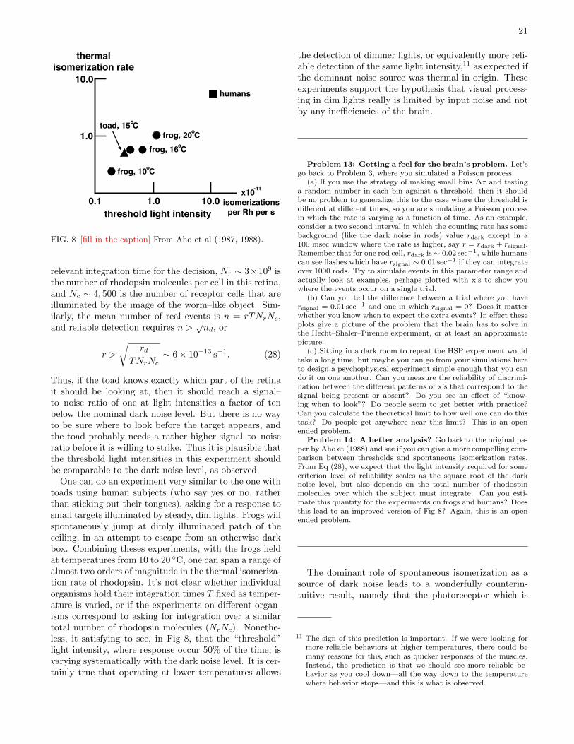
FIG. 8 [fill in the caption] From Aho et al (1987, 1988).

relevant integration time for the decision, Nr ! 3(109 isthe number of rhodopsin molecules per cell in this retina,and Nc ! 4, 500 is the number of receptor cells that areilluminated by the image of the worm–like object. Sim-ilarly, the mean number of real events is n = rTNrNc,and reliable detection requires n >

&nd, or

r >

'rd

TNrNc! 6( 10!13 s!1. (28)

Thus, if the toad knows exactly which part of the retinait should be looking at, then it should reach a signal–to–noise ratio of one at light intensities a factor of tenbelow the nominal dark noise level. But there is no wayto be sure where to look before the target appears, andthe toad probably needs a rather higher signal–to–noiseratio before it is willing to strike. Thus it is plausible thatthe threshold light intensities in this experiment shouldbe comparable to the dark noise level, as observed.

One can do an experiment very similar to the one withtoads using human subjects (who say yes or no, ratherthan sticking out their tongues), asking for a response tosmall targets illuminated by steady, dim lights. Frogs willspontaneously jump at dimly illuminated patch of theceiling, in an attempt to escape from an otherwise darkbox. Combining theses experiments, with the frogs heldat temperatures from 10 to 20 $C, one can span a range ofalmost two orders of magnitude in the thermal isomeriza-tion rate of rhodopsin. It’s not clear whether individualorganisms hold their integration times T fixed as temper-ature is varied, or if the experiments on di!erent organ-isms correspond to asking for integration over a similartotal number of rhodopsin molecules (NrNc). Nonethe-less, it satisfying to see, in Fig 8, that the “threshold”light intensity, where response occur 50% of the time, isvarying systematically with the dark noise level. It is cer-tainly true that operating at lower temperatures allows

the detection of dimmer lights, or equivalently more reli-able detection of the same light intensity,11 as expected ifthe dominant noise source was thermal in origin. Theseexperiments support the hypothesis that visual process-ing in dim lights really is limited by input noise and notby any ine"ciencies of the brain.

Problem 13: Getting a feel for the brain’s problem. Let’sgo back to Problem 3, where you simulated a Poisson process.

(a) If you use the strategy of making small bins #! and testinga random number in each bin against a threshold, then it shouldbe no problem to generalize this to the case where the threshold isdi!erent at di!erent times, so you are simulating a Poisson processin which the rate is varying as a function of time. As an example,consider a two second interval in which the counting rate has somebackground (like the dark noise in rods) value rdark except in a100 msec window where the rate is higher, say r = rdark + rsignal.Remember that for one rod cell, rdark is# 0.02 sec"1, while humanscan see flashes which have rsignal # 0.01 sec"1 if they can integrateover 1000 rods. Try to simulate events in this parameter range andactually look at examples, perhaps plotted with x’s to show youwhere the events occur on a single trial.

(b) Can you tell the di!erence between a trial where you haversignal = 0.01 sec"1 and one in which rsignal = 0? Does it matterwhether you know when to expect the extra events? In e!ect theseplots give a picture of the problem that the brain has to solve inthe Hecht–Shaler–Pirenne experiment, or at least an approximatepicture.

(c) Sitting in a dark room to repeat the HSP experiment wouldtake a long time, but maybe you can go from your simulations hereto design a psychophysical experiment simple enough that you cando it on one another. Can you measure the reliability of discrimi-nation between the di!erent patterns of x’s that correspond to thesignal being present or absent? Do you see an e!ect of “know-ing when to look”? Do people seem to get better with practice?Can you calculate the theoretical limit to how well one can do thistask? Do people get anywhere near this limit? This is an openended problem.

Problem 14: A better analysis? Go back to the original pa-per by Aho et (1988) and see if you can give a more compelling com-parison between thresholds and spontaneous isomerization rates.From Eq (28), we expect that the light intensity required for somecriterion level of reliability scales as the square root of the darknoise level, but also depends on the total number of rhodospinmolecules over which the subject must integrate. Can you esti-mate this quantity for the experiments on frogs and humans? Doesthis lead to an improved version of Fig 8? Again, this is an openended problem.

The dominant role of spontaneous isomerization as asource of dark noise leads to a wonderfully counterin-tuitive result, namely that the photoreceptor which is

11 The sign of this prediction is important. If we were looking formore reliable behaviors at higher temperatures, there could bemany reasons for this, such as quicker responses of the muscles.Instead, the prediction is that we should see more reliable be-havior as you cool down—all the way down to the temperaturewhere behavior stops—and this is what is observed.

22

designed to maximize the signal–to–noise ratio for de-tection of dim lights will allow a significant number ofphotons to pass by undetected. Consider a rod photore-ceptor cell of length &, with concentration C of rhodopsin;let the absorption cross section of rhodopsin be #. [DoI need to explain the definition of cross sections, and/orthe derivation of Beer’s law?] As a photon passes alongthe length of rod, the probability that it will be absorbed(and, presumably, counted) is p = 1 " exp("C#&), sug-gesting that we should make C or & larger in order tocapture more of the photons. But, as we increase C or&, we are increasing the number of rhodopsin molecules,Nrh = CA&, with A the area of the cell, so we we alsoincrease the rate of dark noise events, which occurs at arate rdark per molecule.

If we integrate over a time ' , we will see a mean num-ber of dark events (spontaneous isomerizations) ndark =rdark'Nrh. The actual number will fluctuate, with a stan-dard deviation (n =

&ndark. On the other hand, if

nflash photons are incident on the cell, the mean numbercounted will be ncount = nflashp. Putting these factorstogether we can define a signal–to–noise ratio

SNR ) ncount

(n= nflash

[1" exp("C#&)]&CA&rdark'

. (29)

The absorption cross section # and the spontaneous iso-merization rate rdark are properties of the rhodopsinmolecule, but as the rod cell assembles itself, it can adjustboth its length & and the concentration C of rhodopsin;in fact these enter together, as the product C&. WhenC& is larger, photons are captured more e"ciently andthis leads to an increase in the numerator, but there alsoare more rhodopsin molecules and hence more dark noise,which leads to an increase in the denominator. Viewedas a function of C&, the signal–to–noise ratio has a max-imum at which these competing e!ects balance; workingout the numbers one finds that the maximum is reachedwhen C& ! 1.26/#, and we note that all the other param-eters have dropped out. In particular, this means thatthe probability of an incident photon not being absorbedis 1 " p = exp("C#&) ! e!1.26 ! 0.28. Thus, to maxi-mize the signal–to–noise ratio for detecting dim flashes oflight, nearly 30% of photons should pass through the rodwithout being absorbed (!). Say something about howthis compares with experiment!

Problem 15: Escape from the tradeo!. Derive for yourselfthe numerical factor (C))opt # 1.26/'. Can you see any way todesign an eye which gets around this tradeo! between more e"cientcounting and extra dark noise? Hint: Think about what you seelooking into a cat’s eyes at night.

0 0.5 1 1.5 2 2.5 30

0.5

1

1.5

2

2.5

3

mean rating of flashes at fixed intensity

0 1 2 30

1

2

variance of

ratings

0 1 2 3 4 5 6 7

0

0.05

0.1

0.15

0.2

0.25

0.3

0.35

!!" " !" #" $" %" &" '" (" )""

"*&

!

!*&

#

#*&

$

0 30 600

1

2

mean

rating0 1 2 3 4 5 6

intensity

0

0.1

0.2

rating

probability

FIG. 9 Results of experiments in which observers are askedto rate the intensity of dim flashes, including blanks, on ascale from 0 to 6. Main figure shows that the variance of theratings at fixed intensity is equal to the mean, as expected ifthe ratings are Poisson distributed. Insets show that the fulldistribution is approximately Poisson (upper) and that themean rating is linearly related to the flash intensity, measuredhere as the mean number of photons delivered to the cornea.From Sakitt (1972).

If this is all correct, it should be possible to coax humansubjects into giving responses that reflect the countingof individual photons, rather than just the summationof multiple counts up to some threshold of confidence orreliability. Suppose we ask observers not to say yes or no,but rather to rate the apparent intensity of the flash, sayon a scale from 0 to 7. Remarkably, as shown in Fig 9,in response to very dim flashes interspersed with blanks,at least some observers will generate rating that, giventhe intensity, are approximately Poisson distributed: thevariance of the ratings is essentially equal to the mean,and even the full distribution of ratings over hundredsof trials is close to Poisson. Further, the mean rating islinearly related to the light intensity, with an o!set thatagrees with other measurements of the dark noise level.Thus, the observers behaves exactly as if she can give arating that is equal to the number of photons counted.This astonishing result would be almost too good to betrue were it not that some observers deviate from thisideal behavior—they starting counting at two or three,but otherwise follow all the same rules.While the phenomena of photon counting are very

beautiful, one might worry that this represents just avery small corner of vision. Does the visual system con-tinue to count photons reliably even when it’s not com-pletely dark outside? To answer this let’s look at visionin a rather di!erent animal, as in Fig 10. When you lookdown on the head of a fly, you see—almost to the exclu-sion of anything else—the large compound eyes. Eachlittle hexagon that you see on the fly’s head is a sepa-

23

FIG. 10 The fly’s eye(s). At left a photograph taken by HLeertouwer at the Rijksuniversiteit Groningen, showing (evenin this poor reproduction) the hexagonal lattice of lenses inthe compound eye. This is the blowfly Calliphora vicina. Atright, a schematic of what a fly might see, due to Gary Larson.The schematic is incorrect because each lens actually looks ina di!erent direction, so that whole eye (like ours) only hasone image of the visual world. In our eye the “pixelation”of the image is enforced by the much less regular lattice ofreceptors on the retina; in the fly pixelation occurs alreadywith the lenses.

rate lens, and in large flies there are ! 5, 000 lenses ineach eye, with approximately 1 receptor cell behind eachlens, and roughly 100 brain cells per lens devoted to theprocessing of visual information. The lens focuses lighton the receptor, which is small enough to act as an op-tical waveguide. Each receptor sees only a small portionof the world, just as in our eyes; one di!erence betweenflies and us is that di!raction is much more significantfor organisms with compound eyes—because the lensesare so small, flies have an angular resolution of about 1$,while we do about 100( better. [Add figure to emphasizesimilarity of two eye types.]

The last paragraph was a little sloppy (“approximatelyone receptor cell”?), so let’s try to be more precise. Forflies there actually are eight receptors behind each lens.Two provide sensitivity to polarization and some colorvision, which we will ignore here. The other six receptorslook out through the same lens in di!erent directions, butas one moves to neighboring lenses one finds that there isone cell under each of six neighboring lenses which looksin the same direction. Thus these six cells are equivalentto one cell with six times larger photon capture crosssection, and the signals from these cells are collected andsummed in the first processing stage (the lamina); onecan even see the expected six fold improvement in signalto noise ratio, in experiments we’ll describe shortly.12

Because di!raction is such a serious limitation, onemight expect that there would be fairly strong selection

12 Talk about the developmental biology issues raised by these ob-servations, and the role of the photoreceptors as a model systemin developmental decision making. For example, Lubensky et al(2011). Not sure where to put this, though.

for eyes that make the most of the opportunities withinthese constraints. Indeed, there is a beautiful literatureon optimization principles for the design of the compoundeye; the topic even makes an appearance in Feynman’sundergraduate physics lectures. Roughly speaking (Fig11), we can think of the fly’s head as being a sphere ofradius R, and imagine that the lens are pixels of lineardimension d on the surface. Then the geometry deter-mines an angular resolution (in radians) of ()geo ! d/R;resolution gets better if d gets smaller. On the otherhand, di!raction through an aperture of size d creates ablur of angular width ()di! ! */d, where * ! 500 nmis the wavelength of the light we are trying to image;this limit of course improves as the aperture size d getslarger. Although one could try to give a more detailedtheory, it seems clear that the optimum is reached whenthe two di!erent limits are about equal, corresponding toan optimal pixel size

d# !&*R. (30)

This is the calculation in the Feynman lectures, andFeynman notes that it gives the right answer within 10%in the case of a honey bee.A decade before Feynman’s lectures, Barlow had de-

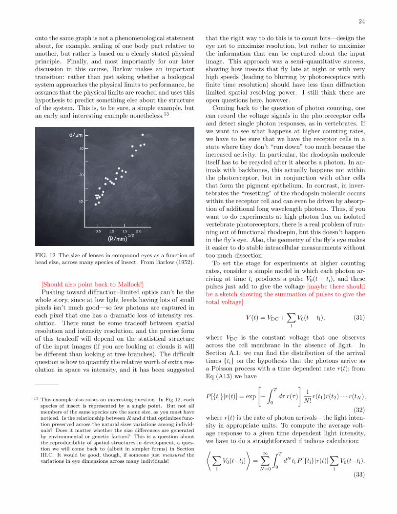
rived the same formula and went into the drawers of thenatural history museum in Cambridge to find a varietyof insects with varying head sizes, and he verified thatthe pixel size really does scale with the square root ofthe head radius, as shown in Fig 12. I think this workshould be more widely appreciated, and it has several fea-tures we might like to emulate. First, it explicitly bringsmeasurements on many species together in a quantita-tive way. Second, the fact that multiple species can put

FIG. 11 At left, a schematic of the compound eye, with lensesof width d on the surface of a spherical eye with radius R. Atright, the angular resolution of the eye as a function of thelens size, showing the geometric ("#geo ! d/R) and di!raction("#di! ! $/d) contributions in dashed lines; the full resolutionin solid lines.

24

onto the same graph is not a phenomenological statementabout, for example, scaling of one body part relative toanother, but rather is based on a clearly stated physicalprinciple. Finally, and most importantly for our laterdiscussion in this course, Barlow makes an importanttransition: rather than just asking whether a biologicalsystem approaches the physical limits to performance, heassumes that the physical limits are reached and uses thishypothesis to predict something else about the structureof the system. This is, to be sure, a simple example, butan early and interesting example nonetheless.13

0.5 1.0 1.5 2.0

(R/mm)1/2

10

20

30

d/µm

FIG. 12 The size of lenses in compound eyes as a function ofhead size, across many species of insect. From Barlow (1952).

[Should also point back to Mallock!]Pushing toward di!raction–limited optics can’t be the

whole story, since at low light levels having lots of smallpixels isn’t much good—so few photons are captured ineach pixel that one has a dramatic loss of intensity res-olution. There must be some tradeo! between spatialresolution and intensity resolution, and the precise formof this tradeo! will depend on the statistical structureof the input images (if you are looking at clouds it willbe di!erent than looking at tree branches). The di"cultquestion is how to quantify the relative worth of extra res-olution in space vs intensity, and it has been suggested

13 This example also raises an interesting question. In Fig 12, eachspecies of insect is represented by a single point. But not allmembers of the same species are the same size, as you must havenoticed. Is the relationship between R and d that optimizes func-tion preserved across the natural sizes variations among individ-uals? Does it matter whether the size di!erences are generatedby environmental or genetic factors? This is a question aboutthe reproducibility of spatial structures in development, a ques-tion we will come back to (albeit in simpler forms) in SectionIII.C. It would be good, though, if someone just measured thevariations in eye dimensions across many individuals!

that the right way to do this is to count bits—design theeye not to maximize resolution, but rather to maximizethe information that can be captured about the inputimage. This approach was a semi–quantitative success,showing how insects that fly late at night or with veryhigh speeds (leading to blurring by photoreceptors withfinite time resolution) should have less than di!ractionlimited spatial resolving power. I still think there areopen questions here, however.Coming back to the question of photon counting, one

can record the voltage signals in the photoreceptor cellsand detect single photon responses, as in vertebrates. Ifwe want to see what happens at higher counting rates,we have to be sure that we have the receptor cells in astate where they don’t “run down” too much because theincreased activity. In particular, the rhodopsin moleculeitself has to be recycled after it absorbs a photon. In an-imals with backbones, this actually happens not withinthe photoreceptor, but in conjunction with other cellsthat form the pigment epithelium. In contrast, in inver-tebrates the “resetting” of the rhodopsin molecule occurswithin the receptor cell and can even be driven by absorp-tion of additional long wavelength photons. Thus, if youwant to do experiments at high photon flux on isolatedvertebrate photoreceptors, there is a real problem of run-ning out of functional rhodospin, but this doesn’t happenin the fly’s eye. Also, the geometry of the fly’s eye makesit easier to do stable intracellular measurements withouttoo much dissection.To set the stage for experiments at higher counting

rates, consider a simple model in which each photon ar-riving at time ti produces a pulse V0(t " ti), and thesepulses just add to give the voltage [maybe there shouldbe a sketch showing the summation of pulses to give thetotal voltage]

V (t) = VDC +!

i

V0(t" ti), (31)

where VDC is the constant voltage that one observesacross the cell membrane in the absence of light. InSection A.1, we can find the distribution of the arrivaltimes {ti} on the hypothesis that the photons arrive asa Poisson process with a time dependent rate r(t); fromEq (A13) we have

P [{ti}|r(t)] = exp

("% T

0d' r(')

)1

N !r(t1)r(t2) · · · r(tN ),

(32)where r(t) is the rate of photon arrivals—the light inten-sity in appropriate units. To compute the average volt-age response to a given time dependent light intensity,we have to do a straightforward if tedious calculation:

*!

i

V0(t"ti)

+=

"!

N=0

% T

0dN ti P [{ti}|r(t)]

!

i

V0(t"ti).

(33)

25

This looks a terrible mess. Actually, it’s not so bad, andone can proceed systematically to do all of the integrals.Once you have had some practice, this isn’t too di"cult,but the first time through it is a bit painful, so I’ll pushthe details o! into Section A.1, along with all the otherdetails about Poisson processes. When the dust settles[leading up to Eq (A64)], the voltage responds linearlyto the light intensity,

#V (t)$ = VDC +

% "

!"dt%V0(t" t%)r(t%). (34)

In particular, if we have some background photon count-ing rate r that undergoes fractional modulations C(t), sothat

r(t) = r[1 + C(t)], (35)

then there is a linear response of the voltage to the con-trast C,

##V (t)$ = r

% "

!"dt%V0(t" t%)C(t%). (36)

Recall that such integral relationships (convolutions)simplify when we use the Fourier transform. For a func-tion of time f(t) we will define the Fourier transform withthe conventions

f(!) =

% "

!"dt e+i#tf(t), (37)

f(t) =

% "

!"

d!

2$e!i#tf(!). (38)

Then, for two functions of time f(t) and g(t), we have

% "

!"dt e+i#t

#% "

!"dt% f(t" t%)g(t%)

$= f(!)g(!). (39)

Problem 16: Convolutions. Verify the “convolution theo-rem” in Eq (39). If you need some reminders, see, for example,Lighthill (1958).

Armed with Eq (39), we can write the response of thephotoreceptor in the frequency domain,

##V (!)$ = rV0(!)C(!), (40)

so that there is a transfer function, analogous toimpedance relating current and voltage in an electricalcircuit,

T (!) ) ##V (!)$C(!)

= rV0(!). (41)

Recall that this transfer function is a complex number atevery frequency, so it has an amplitude and a phase,

T (!) = |T (!)|ei$T (#). (42)

The units of T are simply voltage per contrast. The in-terpretation is that if we generate a time varying contrastC(t) = C cos(!t), then the voltage will also vary at fre-quency !,

##V (t)$ = |T (!)|C cos[!t" )T (!)]. (43)

[Should we have one extra problem to verify this lastequation? Or is it obvious?]If every photon generates a voltage pulse V0(t), but the

photons arrive at random, then the voltage must fluctu-ate. To characterize these fluctuations, we’ll use some ofthe general apparatus of correlation functions and powerspectra. A review of these ideas is given in AppendixA.2.We want to analyze the fluctuations of the voltage

around its mean, which we will call (V (t). By definition,the mean of this fluctuation is zero, #(V (t)$ = 0. There isa nonzero variance, #[(V (t)]2$, but to give a full descrip-tion we need to describe the covariance between fluctua-tions at di!erent times, #(V (t)(V (t%)$. Importantly, weare interested in systems that have no internal clock, sothis covariance or correlation can’t depend separately ont and t%, only on the di!erence. More formally, if we shiftour clock by a time ' , this can’t matter, so we must have

#(V (t)(V (t%)$ = #(V (t+ ')(V (t% + ')$; (44)

this is possible only if

#(V (t)(V (t%)$ = CV (t" t%), (45)

where CV (t) is the “correlation function of V .” Thus,invariance under time translations restricts the form ofthe covariance. Another way of expressing time transla-tion invariance in the description of random functions isto say that any particular wiggle in plotting the functionis equally likely to occur at any time. This property alsois called “stationarity,” and we say that fluctuations thathave this property are stationary fluctuations.

In Fourier space, the consequence of invariance undertime translations can be stated more simply—if we com-pute the covariance between two frequency components,we find

#(V (!1)(V (!2)$ = 2$((!1 + !2)SV (!1), (46)

where SV (!) is called the power spectrum (or power spec-tral density) of the voltage V . Remembering that (V (!)is a complex number, it might be more natural to writethis as

#(V (!1)(V#(!2)$ = 2$((!1 " !2)SV (!1). (47)

26

Time translation invariance thus implies that fluctua-tions at di!erent frequencies are independent.14 Thismakes sense, since if (for example) fluctuations at 2Hzand 3Hz were correlated, we could form beats betweenthese components and generate a clock that ticks everysecond. Finally, the Wiener–Khinchine theorem statesthat the power spectrum and the correlation function area Fourier transform pair,

SV (!) =

%d' e+i#%CV ('), (48)

CV (') =

%d!

2$e!i#%SV (!). (49)

Notice that

#[#V (t)]2$ ) CV (0) =

%d!

2$SV (!). (50)

Thus we can think of each frequency component as hav-ing a variance ! SV (!), and by summing these compo-nents we obtain the total variance.

Problem 17: More on stationarity. Consider some fluctu-ating variable x(t) that depends on time, with )x(t)& = 0. Showthat, because of time translation invariance, higher order correla-tions among Fourier components are constrained:

)x("1)x#("2)x

#("3)& + 2&(("1 ! "2 ! "3) (51)

)x("1)x("2)x#("3)x

#("4)& + 2&(("1 + "2 ! "3 ! "4). (52)

If you think of x# (or x) as being analogous to the operators forcreation (or annihilation) of particles, explain how these relationsare related to conservation of energy for scattering in quantumsystems.

Problem 18: Brownian motion in a harmonic potential.[The harmonic oscillator gets used more than once, of course; checkfor redundancy among problems in di!erent sections!] Consider aparticle of mass m hanging from a spring of sti!ness *, surroundedthrough a fluid. The e!ect of the fluid is, on average, to generate adrag force, and in addition there is a ‘Langevin force’ that describesthe random collisions of the fluid molecules with the particle, re-sulting in Brownian motion. The equation of motion is

md2x(t)

dt2+ +

dx(t)

dt+ *x(t) = ,(t), (53)

where + is the drag coe"cient and ,(t) is the Langevin force. Astandard result of statistical mechanics is that the correlation func-tion of the Langevin force is

),(t),(t$)& = 2+kBT ((t! t$), (54)

where T is the absolute temperature and kB = 1.36 , 10"23 J/Kis Boltzmann’s constant.

(a.) Show that the power spectrum of the Langevin force isS#(") = 2+kBT , independent of frequency. Fluctuations with sucha constant spectrum are called ‘white noise.’

14 Caution: this is true only at second order; it is possible for dif-ferent frequencies to be correlated when we evaluate products ofthree or more terms. See the next problem for an example.

(b.) Fourier transform Eq (53) and solve, showing how x(") isrelated to ,("). Use this result to find an expression for the powerspectrum of fluctuations in x, Sx(").

(c.) Integrate the power spectrm Sx(") to find the total variancein x. Verify that your result agrees with the equipartition theorem,

%1

2*x2

&=

1

2kBT. (55)

Hint: The integral over " can be done by closing a contour in thecomplex plane.

(d.) Show that the power spectrum of the velocity, Sv("), isrelated to the power spectrum of position through

Sv(") = "2Sx("). (56)

Using this result, verify the other prediction of the equipartitiontheorem for this system,

%1

2mv2

&=

1

2kBT. (57)

Now we have a language for describing the signals andnoise in the receptor cell voltage, by going to the fre-quency domain. What does this have to do with countingphotons? The key point is that we can do a calculationsimilar to the derivation of Eq (40) for ##V (t)$ to showthat, at C = 0, the voltage will undergo fluctuations—responding to the random arrival of photons—with powerspectrum

NV (!) = r|V0(!)|2. (58)

We call this NV because it is noise. The noise has aspectrum shaped by the pulses V0, and the magnitude isdetermined by the photon counting rate; again see Ap-pendix A.1 for details.Notice that both the transfer function and noise spec-

trum depend on the details of V0(t). In particular, be-cause this pulse has finite width in time, the transferfunction gets smaller at higher frequencies. Thus if youwatch a flickering light, the strength of the signal trans-mitted by your photoreceptor cells will decrease with in-creasing frequency.The crucial point is that, for an ideal photon counter,

although higher frequency signals are attenuated thesignal–to–noise ratio actually doesn’t depend on fre-quency. Thus if we form the ratio

|T (!)|2

NV (!)=

|rV0(!)|2

r|V0(!)|2= r, (59)

we just recover the photon counting rate, independentof details. Since this is proportional to the signal–to–noise ratio for detecting contrast modulations C(!), weexpect that real photodetectors will give less that thisideal value. [Should be able to make a crisper statementhere—is it a theorem? Prove it, or give the proof as aproblem?]

27

Problem 19: Frequency vs counting rate. [Need to givemore guidance through this problem! Step by step ...] If we arecounting photons at an average rate r, you might think that it iseasier to detect variations in light intensity at a frequency " % rthan at higher frequencies, " " r; after all, in the high frequencycase, the light changes from bright to dim and back even before (onaverage) a single photon has been counted. But Eq (59) states thatthe signal–to–noise ratio for detecting contrast in an ideal photoncounter is independent of frequency, counter to this intuition. Canyou produce a simple simulation to verify the predictions of Eq(59)? As a hint, you should think about observing the photonarrivals over a time T such that rT " 1. Also, if you are lookingfor light intensity variations of the form r(t) = r[1 + C cos("t)],you should process the photon arrival times {ti} to form a signals =

'i cos("ti).

So now we have a way of testing the photoreceptors:Measure the transfer function T (!) and the noise spec-trumNV (!), form the ratio |T (!)|2/NV (!), and comparethis with the actual photon counting rate r. This wasdone for the fly photoreceptors, with the results shown inFig 13. It’s interesting to look back at the original papersand understand how they calibrated the measurement ofr (I’ll leave this as an exercise for you!). [This account ofthe experiments is too glib. I will go back to expand andclarify. Rob has also o!ered new versions of the figures.]

What we see in Fig 13 is that, over some range offrequencies, the performance of the fly photoreceptors isclose to the level expected for an ideal photon counter.It’s interesting to see how this evolves as we change themean light intensity, as shown in Fig 14. The perfor-mance of the receptors tracks the physical optimum up

FIG. 13 Signal and noise in fly photoreceptors, with experi-ments at four di!erent mean light intensities, from de Ruytervan Steveninck & Laughlin (1996b). (a) Transfer function|T (%)|2 from contrast to voltage. (b) Power spectrum ofvoltage noise, NV (%). (c) The ratio |T (%)|2/NV (%), whichwould equal the photon counting rate if the system were ideal;dashed lines show the actual counting rates.

FIG. 14 Performance of fly photoreceptors vs light intensity.[Should redraw this, and label with consistent notation.] Hav-ing measured the quantity $e! = |T (%)|2/NV (%), as in Fig13, we plot the maximum value (typically at relatively lowfrequencies) vs the actual photon counting rate r. We seethat, over an enormous dynamic range, the signal–to–noiseratio tracks the value expected for an ideal photon counter.

to counting rates of r ! 105 photons/s. Since the inte-gration time of the receptors is ! 10ms, this means thatthe cell can count, almost perfectly, up to about 1000.An important point about these results is that they

wouldn’t work if the simple model were literally true. Atlow photon counting rates r, the pulse V0 has an am-plitude of several milliVolts, as you can work out frompanel (a) in Fig 13. If we count ! 103 events, this shouldproduce a signal of several Volts, which is absolutely im-possible in a real cell! What happens is that the systemhas an automatic gain control which reduces the size ofthe pulse V0 as the light intensity is increased. Remark-ably, this gain control or adaptation occurs while pre-serving (indeed, enabling) nearly ideal photon counting.Thus as the lights go up, the response to each photonbecome smaller (and, if you look closely, faster), but noless reliable.

Problem 20: Looking at the data. Explain how the datain Fig 13 provide evidence for the adaption of the pulse V0 withchanges in the mean light intensity.

[This seems a little brief! Maybe there should be asummary of what has happened, what we conclude ...also explain where the loose ends remain vs where thingsare solid.] These observations on the ability of the visualsystem to count single photons—down to the limit set bythermal noise in rhodopsin and up to counting rates of! 105 s!1—raise questions at several di!erent levels:

28

1. At the level of single molecules, we will see thatthe performance of the visual system depends cruciallyon the dynamics of rhodopsin itself. In particular, thestructural response of the molecule to photon absorptionis astonishingly fast, while the dark noise level means thatthe rate of spontaneous structural changes is extremelyslow.2. At the level of single cells, there are challenges in un-

derstanding how a network of biochemical reactions con-verts the structural changes of single rhodopsin moleculesinto macroscopic electrical currents across the rod cellmembrane.3. At the level of the retina as a whole, we would like

to understand how these signals are integrated withoutbeing lost into the inevitable background of noise. Alsoat the level of the retina, we need to understand howsingle photon signals are encoded into the stereotypedpulses that are the universal language of the brain.4. At the level of the whole organism, there are issues

about how the brain learns to make the discriminationsthat are required for optimal performance.In the next sections we’ll look at these questions, in

order.

It is a pleasure to read classic papers, and surely Hecht et al (1942)and van der Velden (1944) are classics, as is the discussion of darknoise by Barlow (1956). The pre–history of the subject, includ-ing the story about Lorentz, is covered by Bouman (1961). Thegeneral idea that our perceptual “thresholds” are really thresholdsfor discrimination against background noise with some criterionlevel of reliability made its way into quantitative psychophysicalexperiments in the 1950s and 60s, and this is now (happily) a stan-dard part of experimental psychology; the canonical treatment isby Green and Swets (1966). The origins of these ideas are an inter-esting mix of physics and psychology, developed largely for radarin during World War II, and a summary of this early work is inthe MIT Radar Lab series (Lawson & Uhlenbeck 1950). Anothernice mix of physics and psychology is the revisiting of the originalphoton counting experiments using light sources with non–Poissonstatistics (Teich et al 1982). The idea that random arrival of pho-tons could limit our visual perception beyond the “just visible” wasexplored, early on, by de Vries (1943) and Rose (1948). Some ofthe early work by de Vries and coworkers on the physics of thesense organs (not just vision) is described in a lovely review (deVries 1956). As a sociological note, de Vries was an experimentalphysicist with very broad interests, from biophysics to radiocarbondating; for a short biography see de Waard (1960).

Barlow 1956: Retinal noise and absolute threshold. HB Barlow,J Opt Soc Am 46, 634–639 (1956).

Bouman 1961: History and present status of quantum theory invision. MA Bouman, in Sensory Communication, W Rosen-blith, ed, pp 377–401 (MIT Press, Cambridge, 1961).

Green & Swets 1966: Signal Detection Theory and Psy-chophysics. DM Green, & JA Swets (Wiley, New York,1966).

Hecht et al 1942: Energy, quanta and vision. S Hecht, S Shlaer& MH Pirenne, J Gen Physiol 25, 819–840 (1942).

Lawson & Uhlenbeck 1950: Threshold Signals. MIT Radia-tion Laboratory Series vol 24 JL Lawson & GE Uhlenbeck(McGraw–Hill, New York, 1950).

Rose 1948: The sensitivity performance of the human eye on anabsolute scale. A Rose, J Opt Soc Am 38, 196–208 (1948).

Teich et al 1982: Multiplication noise in the human visual sys-tem at threshold. III: The role of non–Poisson quantumfluctuations. MC Teich, PR Prucnal, G Vannucci, ME Bre-ton& WJ McGill, Biol Cybern 44, 157–165 (1982).

van der Velden 1944: Over het aantal lichtquanta dat nodig isvoor een lichtprikkel bij het menselijk oog. HA van derVelden, Physica 11, 179–189 (1944).

de Vries 1943: The quantum character of light and its bearingupon threshold of vision, the di!erential sensitivity and vi-sual acuity of the eye. Hl de Vries, Physica 10, 553–564(1943).

de Vries 1956: Physical aspects of the sense organs. Hl de Vries,Prog Biophys Biophys Chem 6, 207–264 (1956).

de Waard 1960: Hessel de Vries, physicist and biophysicist. Hde Waard, Science 131, 1720–1721 (1960).

Single photon responses in receptor cells of the horseshoe crab werereported by Fuortes and Yeandle (1964). The series of papers fromBaylor and co–workers on single photon responses in vertebrate rodcells, first from toads and then from monkeys, again are classics,well worth reading today, not least as examples of how to do quanti-tative experiments on biological systems. Aho, Donner, Reuter andco–workers have made a major e!ort to connect measurements onrod cells and ganglion cells with the behavior of the whole organism,using the toad as an example; among their results are the tempera-ture dependence of dark noise (Fig 8), and the latency/anticipationresults in Section I.D. The remarkable experiments showing thatpeople really can count every photon are by Sakitt (1972). We willlearn more about currents and voltages in cells very soon, but forbackground I have always liked Aidley’s text, now in multiple edi-tions; as is often the case, the earlier editions can be clearer andmore compact.

Aidley 1998: The Physiology of Excitable Cells, 4th Edition DJAidley (Cambridge University Press, Cambridge, 1998).

Aho et al 1987: Retinal noise, the performance of retinal gan-glion cells, and visual sensitivity in the dark00adapted frog.A–C Aho, K Donner, C Hyden, T Reuter & OY Orlov, JOpt Soc Am A 4, 2321–2329 (1987).

Aho et al 1988: Low retinal noise in animals with low body tem-perature allows high visual sensitivity. A–C Aho, K Don-ner, C Hyden, LO Larsen & T Reuter, Nature 334, 348–350(1988).

Aho et al 1993: Visual performance of the toad (Bufo bufo) atlow light levels: retinal ganglion cell responses and prey–catching accuracy. A–C Aho, K Donner, S Helenius, LOLarsen & T Reuter, J Comp Physiol A 172, 671–682 (1993).

Baylor et al 1979a: The membrane current of single rod outersegments. DA Baylor, TD Lamb & K–W Yau, J Physiol(Lond) 288, 589–611 (1979).

Baylor et al 1979b: Rod responses to single photons. DA Bay-lor, TD Lamb & K–W Yau, J Physiol (Lond) 288, 613–634(1979).

Baylor et al 1980: Two components of electrical darm noise intoad retinal rod outer segments. DA Baylor, G Matthews &K–W Yau, J Physiol (Lond) 309, 591–621 (1980).

Baylor et al 1984: The photocurrent, noise and spectral sensi-tivity of rods of the monkey Macaca fascicularis. DA Bay-lor, BJ Nunn & JF Schnapf, J Physiol (Lond) 357, 575–607(1984).

Fuortes & Yeandle 1964: Probability of occurrence of discretepotential waves in the eye of Limulus. MGF Fuortes & SYeandle, J Gen Physiol 47, 443–463 (1964).

Sakitt 1972: Counting every quantum. B Sakitt, J Physiol 223,131–150 (1972).

29

For the discussion of compound eyes, useful background is con-tained in Stavenga and Hardie (1989), and in the beautiful com-pilation of insect brain anatomy by Strausfeld (1976), althoughthis is hard to find; as an alternative there is an online atlas,http://flybrain.neurobio.arizona.edu/Flybrain/html/. Thereis also the more recent Land & Nilsson (2002). Evidently Larson(2003) is an imperfect guide to these matters. Everyone should havea copy of the Feynman lectures (Feynman et al 1963), and checkthe chapters on vision. The early work by Barlow (1952) deservesmore appreciation, as noted in the main text, and the realizationthat di!raction must be important for insect eyes goes back toMallock (1894). For a gentle introduction to the wider set of ideasabout scaling relations between di!erent body parts, see McMa-hon & Bonner (1983). The experiments on signal–to–noise ratio infly photoreceptors are by de Ruyter van Steveninck and Laughlin(1996a, 1996b). For a review of relevant ideas in Fourier analysisand related matters, see Appendix A.2 and Lighthill (1958). Youshould come back to the ideas of Snyder et al (Snyder 1977, Snyderet al 1977) near the end of the book, after we have covered someof the basics of information theory.

Barlow 1952: The size of ommatidia in apposition eyes. HB Bar-low, J Exp Biol 29, 667–674 (1952).

Feynman et al 1963: The Feynman Lectures on Physics. RPFeynman, RB Leighton & M Sands (Addison–Wesley, Read-ing, 1963).

Larson 2003: The Complete Far Side. G Larson (Andrews Mc-Neel Publishing, Kansas City, 2003).

Land & Nilsson 2002: Animal Eyes MF Land & D–E Nilsson(Oxford University Press, Oxford, 2002).

Lighthill 1958: Introduction to Fourier Analysis and GeneralizedFunctions. MJ Lighthill (Cambridge University Press, Cam-bridge, 1958)

Mallock 1894: Insect sight and the defining power of compositeeyes. A Mallock, Proc R Soc Lond 55, 85–90 (1894).

McMahon & Bonner 1983: On Size and Life. TA McMahon& JT Bonner (WH Freeman, New York, 1983).

de Ruyter van Steveninck & Laughlin 1996a: The rate ofinformation transfer at graded–potential synapses. RR deRuyter van Steveninck & SB Laughlin, Nature 379, 642–645 (1996).

de Ruyter van Steveninck & Laughlin 1996b: Light adap-tation and reliability in blowfly photoreceptors. R de Ruytervan Steveninck & SB Laughlin, Int. J. Neural Syst. 7, 437–444 (1996)

Snyder 1977: Acuity of compound eyes: Physical limitations anddesign. AW Snyder, J Comp Physiol 116, 161–182 (1977).

Snyder et al 1977: Information capacity of compound eyes. AWSnyder, DS Stavenga & SB Laughlin, J Comp Physiol 116,183–207 (1977).

Stavenga & Hardie 1989: Facets of Vision. DG Stavenga &RC Hardie, eds (Springer–Verlag, Berlin, 1989).

Strausfeld 1976: Atlas of an Insect Brain. N Strausfeld(Springer–Verlag, Berlin, 1976).

Finally, a few reviews that place the results on photon countinginto a broader context.

Barlow 1981: Critical limiting factors in the design of the eyeand visual cortex. HB Barlow, Proc R Soc Lond Ser B 212,1–34 (1981).

Bialek 1987: Physical limits to sensation and perception. WBialek, Ann Rev Biophys Biophys Chem 16, 455–478 (1987).

Rieke & Baylor 1998: Single photon detection by rod cells ofthe retina. F Rieke & DA Baylor, Rev Mod Phys 70, 1027–1036 (1998).

11

12

retinal(11-cis)

opsin protein

C

C

CH

H=

CCC

H

=

FIG. 15 Schematic structure of rhodopsin, showing the or-ganic pigment retinal nestled in a pocket formed by the sur-rounding opsin protein. This conformation of the retinal iscalled 11–cis, since there is a rotation around the bond be-tween carbons numbered 11 and 12 (starting at the lower rightin the ring). Insets illustrate the conventions in such chemicalstructures, with carbons at nodes of the skeleton, and hydro-gens not shown, but su"cient to make sure that each carbonforms four bonds.

B. Single molecule dynamics

To a remarkable extent, our ability to see in the darkis limited by the properties of rhodopsin itself, essen-tially because everything else works so well. Rhodopsinconsists of a medium sized organic pigment, retinal, en-veloped by a large protein, opsin (cf Fig 15). The pri-mary photo–induced reaction is isomerization of the reti-nal, which ultimately couples to structural changes in theprotein. The e!ort to understand the dynamics of theseprocesses goes back to Wald’s isolation of retinal (a vi-tamin A derivative) in the 1930s, his discovery of theisomerization, and the identification of numerous statesthrough which the molecule cycles. The field was givena big boost by the discovery that there are bacterialrhodopsins, some of which serve a sensory function whileothers are energy transducing molecules, using the en-ergy of the absorbed photon to pump protons across thecell membrane; the resulting di!erence in electrochem-ical potential for protons is a universal intermediate incellular energy conversion, not just in bacteria but in usas well. [Maybe a pointer to channel rhodopsins wouldbe good here too.]By now we know much more than Wald did about the

structure of the rhodopsin molecule [need to point to abetter figure, more details].While there are many remarkable features of the

rhodopsin molecule, we would like to understand thoseparticular features that contribute to the reliability ofphoton counting. First among these is the very low spon-taneous isomerization rate, roughly once per thousandyears. As we have seen, these photon–like events provide

30

11

12

11-cis

11

12

all-trans

cis-trans

isomerization

FIG. 16 Isomerization of retinal, the primary event at thestart of vision. The &–bonds among the carbons favor pla-nar structures, but there are still alternative conformations.The 11–cis conformation is the ground state of rhodopsin,and after photon absorption the molecule converts to the all–trans configuration. These di!erent structures have di!erentabsorption spectra, as well as other, more subtle di!erences.Thus we can monitor the progress of the transition 11–cis "all–trans essentially by watching the molecule change color,albeit only slightly. [Show the spectra!]

the dominant noise source that limits our ability to see inthe dark, so there is a clear advantage to having the low-est possible rate. When we look at the molecules them-selves, purified from the retina, we can “see” the isomer-ization reaction because the initial 11–cis state and thefinal all–trans states (see Fig 16) have di!erent absorp-tion spectra [add this to the figure]. For rhodopsin itself,the spontaneous isomerization rate is too slow to observein a bulk experiment. If we isolate the pigment retinal,however, we find that it has a spontaneous isomerizationrate of ! 1/yr, so that a bottle of 11–cis retinal is quitestable, but the decay to all–trans is observable.

How can we understand that rhodopsin has a spon-taneous isomerization rate 1000( less than that of reti-nal? The spontaneous isomerization is thermally acti-vated, and has a large “activation energy” as estimatedfrom the temperature dependence of the dark noise.15

It seems reasonable that placing the retinal moleculeinto the pocket formed by the protein opsin would raisethe activation energy, essentially because parts of theprotein need to be pushed out of the way in orderfor the retinal to rotate and isomerize. Although thissounds plausible, it’s probably wrong. If we write the

15 I am assuming here that the ideas of activation energy and Arrhe-nius behavior of chemical reaction rates are familiar. For moreon this, see Section II.A.

dark isomerization rate as r = Ae!Eact/kBT , retinal andrhodopsin have the same value of the activation energyEact = 21.9 ± 1.6 kcal/mole [this is from measurementson rods; give the number in useful units! maybe foot-note about di"culties of units] within experimental er-ror, but di!erent values of the prefactor A. If we look atphotoreceptor cells that are used for daytime vision—thecones, which also provide us with sensitivity to colors, asdiscussed below [check where this gets done!]—the darknoise level is higher (presumably single photon countingis unnecessary in bright light), but again this is a di!er-ence in the prefactor, not in the activation energy. Aswe will see when we discuss the theory of reaction ratesin Section II.A, understanding prefactors is much harderthan understanding activation energies, and I think wedon’t really have a compelling theoretical picture that ex-plains the di!erence between retinal and rhodopsin.[FredRieke gave me some pointers I have to chase down beforedeciding on that last sentence!]The isolated retinal pigment isomerization at a rate

that is faster than rhodopsin. On the other hand, ifwe excite the isolated retinal with a very short pulse oflight, and follow the resulting changes in absorption spec-trum, these photo–induced dynamics are not especiallyfast, with isomerization occurring at a rate ! 109 s!1.Although this is fast compared to the reactions that wecan see directly, it is actually so slow that it is com-parable to the rate at which the molecule will re–emitthe photon. We recall from quantum mechanics that thespontaneous emission rates from electronic excited statesare constrained by sum rules if they are dipole–allowed.This means that emission lifetimes for visible photons areorder 1 nanosecond for almost all of the simple cases. Ina big molecule, there can be some re–arrangement of themolecular structure before the photon is emitted (see thediscussion below), and this results in the emitted or fluo-rescent photon being of longer wavelength. Nonetheless,the natural time scale is nanoseconds, and the isomeriza-tion of retinal is not fast enough to prevent fluorescenceand truly capture the energy of the photon with highprobability.

Problem 21: Why nanoseconds? Explain why spontaneousemission of visible photons typically occurs with a rate # 109 s"1.[Need to explain where to start!]

Now fluorescence is a disaster for visual pigment—notonly don’t you get to count the photon where it was ab-sorbed, it might get counted somewhere else, blurring theimage. In fact rhodopsin does not fluoresce: The quan-tum yield or branching ratio for fluorescence is ! 10!5.

31

FIG. 17 [This needs to be redrawn; maybe two figures tomake di!erent points? Convert all the units once and for all?]Femtosecond dynamics of rhodopsin, from Wang et al (1994).At left, schematic potential energy surfaces in the electronicground and excited states. At right, panel (A) shows tran-sient absorption spectra following a 35 fs pulse of 500 nm light.Panel (B) shows the magnitude of the Fourier transform ofthe time dependent absorption at each of several wavelengths,illustrating the oscillations expected if the vibrational dynam-ics is coherent. You might like to convert the kcal/mol andcm"1 into more conventional physical units!

If we imagine the molecule sitting in the excited state,transitioning to the ground state via fluorescence at arate ! 109 s!1, then to have a branching ratio of 10!5 thecompeting process must have a rate of ! 1014 s!1. Thus,the rhodopsin molecule must leave the excited state bysome process on a time scale of ! 10 femtoseconds, whichis extraordinarily fast. Indeed, for many years, everytime people built faster pulsed lasers, they went back torhodopsin to look at the initial events, culminating in thedirect demonstration of femtosecond isomerization, mak-ing this one of the fastest molecular events ever observed.

The 11–cis and all trans configurations of retinal havedi!erent absorption spectra, and this is why we can ob-serve the events following photon absorption as an evo-lution of the spectrum. The basic design of such ex-periments is to excite the molecules with a brief pulseof light, elevating them into the excited state, and thenprobe with another brief pulse after some delay. In thesimplest version, one repeats the experiment many timeswith di!erent choices of the delay and the energy or wave-length of the probe pulse. An example of the results fromsuch an experiment are shown in Fig 17. The first thingto notice is that the absorption at a wavelength of 550 nm,characteristic of the all–trans structure, rises very quicklyafter the pulse which excites the system, certainly withintens of femtoseconds. In fact this experiment reveals allsorts of interesting structure, to which we will return be-low.

The combination of faster photon induced isomeriza-tion and slower thermal isomerization means that the

protein opsin acts as an electronic state selective cata-lyst: ground state reactions are inhibited, excited statereactions accelerated, each by orders of magnitude. It isfair to say that if these state dependent changes in re-action rate did not occur—that is, if the properties ofrhodopsin were those of retinal—then we simply wouldnot be able to see in the dark of night.

Problem 22: What would vision be like if ... ? Imagine thatthe spontaneous isomerization rate and quantum yield for photo–isomerization in rhodopsin were equal to those in retinal. Estimate,quantitatively, what this would mean for our ability to see at night.[we should try to connect with real intensities at dusk etc.]

In order to make sense out of all of this, and get startedin understanding how rhodopsin achieves its function, weneed to understand something about electronic transi-tions in large molecules, as opposed to the case of atomsthat we all learned about in our quantum mechanicsclasses. The absorption of a photon by an atom involvesa transition between two electronic states, and this is alsotrue for a large molecule. But for the atom the absorp-tion line is very narrow, while for big molecules it is verybroad. For rhodopsin, there is a nice of way of measur-ing the absorption spectrum over a very large dynamicrange, and this is to use the rod cell as a sensor. In-stead of asking how much light is absorbed, we can tryassuming16 that all absorbed photons have a constantprobability of generating a pulse of current at the rod’soutput, and so we can adjust the light intensity at eachwavelength to produce the same current. If the absorp-tion is stronger, we need less light, and conversely morelight if the absorption is weaker. The results of such anexperiment are shown in Fig 18. It is beautiful that inthis way one can follow the long wavelength tail of thespectrum down to cross–sections that are ! 10!5 of thepeak. More qualitatively, we see that the width of thespectrum, say at half maximum, is roughly 20% of thepeak photon energy, which is enormous in contrast withatomic absorption lines.As an aside, the fact that one can follow the sensitivity

of the photoreceptor cell deep into the long wavelengthtail opens the possibility of asking a very di!erent ques-tion about the function of these cells (and all cells). Werecall that every cell in our bodies has the same genetic

16 This assumption can also be checked. It’s true, but I think therehave not been very careful measurements in the long wavelengthtail, where something interesting might happen.

32

material, and hence the instructions for making all pos-sible proteins. In particular, all photoreceptor cells havethe ability to make all visual pigments. But the di!erentclasses of receptors—rods and the three kinds of cones—make di!erent pigments, corresponding to di!erent pro-teins surrounding more or less the same retinal molecule,and the resulting di!erences in absorption spectra pro-vide the basis for color vision. If a single cone couldn’treliably turn on the expression of one rhodopsin gene,and turn o! all of the others, then the retina wouldn’tbe able to generate a mix of spectral sensitivities, and wewouldn’t see colors. But how “o!” is “o!”?

In a macaque monkey (not so di!erent from us in thesematters), “red” cones have their peak sensitivity at awavelength ! 570 nm, but at this wavelength the “blue”cones have sensitivities that are ! 105( reduced rela-tive to their own peak. Since the peak absorption cross–sections are comparable, this tells us that the relativeconcentration of red pigments in the blue cones must beless than 10!5. That is, the cell makes at least 105 timesas much of the correct protein as it does of the incorrectproteins, which I always thought was pretty impressive.17

Returning to the absorption spectrum itself, we realizethat a full treatment would describe molecules by doing

Relative

sensitivity

0.1

0.01

0.001

0.0001

1

400 500 600 700

wavelength (nm)

FIG. 18 Sensitivity of the rod photoreceptor as a function ofwavelength. This is measured, as explained in the text, byadjusting the intensity of light to give a criterion output, sothat very low sensitivity corresponds to shining a bright light,rather than measuring a small output. Redrawn from Bayloret al (1979a).

17 Many thanks to Denis Baylor for reminding me of this argument.Since there are # 109 rhodopsins in one cell, errors of even onepart in 105 would mean that there are thousands of “wrong”molecules floating around. I wonder if this is true, or if the trueerrors are even smaller. [Apparently there is evidence that somecones are less precise about what defines “o!;” should check this!]

FIG. 19 Schematic of the electronic states in a large molecule,highlighting their coupling to motion of the nuclei. The sketchshow two states, with photon absorption (in blue) drivingtransitions between them. If we think in semi–classical terms,as explained in the text, then these transitions are ‘too fast’for the atoms to move, and hence are vertical on such plots(the Franck–Condon approximation). Because the atomic co-ordinates fluctuate, as indicated by the Boltzmann distribu-tion, the energy of the photon required to drive the transitionalso fluctuates, and this broadens the absorption spectrum.

the quantum mechanics of a combined system of elec-trons and nuclei. But the nuclei are very much heavierthan the electrons, and hence move more slowly. Morerigorously, the large ratio of masses means that we canthink of solving the quantum mechanics of the electronswith the nuclei in fixed position, and then for each suchatomic configuration the energy of the electrons con-tributes to the potential energy; as the nuclei move inthis potential (whether classically or quantum mechan-ically) the electrons follow adiabatically.18 This is theBorn–Oppenheimer approximation, which is at the heartof all attempts to understand molecular dynamics.19

Figure 19 shows the energy of two di!erent electronicstates, plotted schematically against (one of the) atomiccoordinates. In the ground state, we know that there issome arrangement of the atoms that minimizes the en-

18 Because the electrons (mostly) follow the nuclei, I will use “nu-clei” and “atoms” interchangeably in what follows.

19 I assume that most readers know something about the Born–Oppenheimer approximation, since it is a pretty classical subject.It is also one of the first adiabatic approximations in quantummechanics. It took many years to realize that some very in-teresting things can happen in the adiabatic limit, notably theappearance of non–trivial phase factors in the adiabatic evolu-tion of wave functions. Some of these ‘complications’ (to use aword from one of original papers) were actually discovered in thecontext of the Born–Oppenheimer approximation itself, but nowwe know that this circle of ideas is much bigger, extending outto quantum optics and quite exotic field theories.

33

ergy, and that in the neighborhood of this minimum thepotential surface must look roughly like that of a systemof Hookean springs. Once we lift the electrons into thefirst excited state, there is again some configuration ofthe atoms that minimizes the energy (unless absorbingone photon is enough to break the molecule apart!), butunless there is some symmetry this equilibrium configu-ration will be di!erent than in the ground state, and thesti!ness of the spring holding the molecule in this equi-librium configuration also will be di!erent. Hence in Fig19, the energy surfaces for the ground and excited statesare shown displaced and with di!erent curvatures.

It is important to realize that sketches such as that inFig 19 are approximations in many senses. Most impor-tantly, this sketch involves only one coordinate. You maybe familiar with a similar idea in the context of chemicalreactions, where out of all the atoms that move duringthe reaction we focus on one “reaction coordinate” thatforms a path from the reactants to products; for moreabout this see Section II.A. One view is that this isjust a convenience—we can’t draw in many dimensions,so we just draw one, and interpret the figure cautiously.Another view is that the dynamics are e!ectively one di-mensional, either because there is a separation of timescales, or because we can change coordinates to isolate,for example, a single coordinate that couples to the di!er-ence in energy between the ground and excited electronicstates. The cost of this reduction in dimensionality mightbe a more complex dynamics along this one dimension,for example with a “viscosity” that is strongly frequencydependent, which again means that we need to be cau-tious in interpreting the picture that we draw. In whatfollows I’ll start by being relatively informal, and try tobecome more precise as we go along.

In the limit that the atoms are infinitely heavy, theydon’t move appreciably during the time required for anelectronic transition. On the other hand, the positionsof the atoms still have to come out of the Boltzmanndistribution, since the molecule is in equilibrium withits environment at temperature T . In this limit, we canthink of transitions between electronic states as occurringwithout atomic motion, corresponding to vertical lineson the schematic in Fig 19. If the photon happens to ar-rive when the atomic configuration is a bit to the left ofthe equilibrium point, then as drawn the photon energyneeds to be larger in order to drive the transition; if theconfiguration is a bit to the right, then the photon en-

ergy is smaller. In this way, the Boltzmann distributionof atomic positions is translated into a broadening of theabsorption line. In particular, the transition can occurwith a photon that has very little energy if we happento catch a molecule in the rightward tail of the Boltz-mann distribution: the electronic transition can be madeup partly from the energy of the photon and partly fromenergy that is “borrowed” from the thermal bath. As aresult, the absorption spectrum should have a tail at longwavelengths, and this tail will be strongly temperaturedependent, and this is observed in rhodopsin and otherlarge molecules. Since our perception of color depends onthe relative absorption of light by rhodopsins with di!er-ent spectra, this means that there must be wavelengthssuch that the apparent color of the light will depend ontemperature [need a pointer and refs for this .. maybetell the story of de Vries and the hot tub?]Concretely, if we imagine that the potential surfaces

are perfect Hookean springs, but with displaced equilib-rium positions, then we can relate the width of the spec-trum directly to the magnitude of this displacement. Inthe ground state we have the potential

Vg(q) =1

2+q2, (60)

and in the excited state we have

Ve(q) = ,+1

2+(q "#)2, (61)

where , is the minimum energy di!erence between thetwo electronic states and # is the shift in the equilib-rium position, as indicated in Fig 20. With q fixed, thecondition for absorbing a photon is that the energy !$match the di!erence in electronic energies,

!$ = Ve(q)" Vg(q) = ,+1

2+#2 " +#q. (62)

The probability distribution of q when molecules are inthe ground state is given by

P (q) =1

Zexp

#"Vg(q)

kBT

$=

1"2$kBT/+

exp

#" +q2

2kBT

$,

(63)so we expect the cross–section for absorbing a photon offrequency $ to have the form

#($) *%

dq P (q)(

#!$"

,,+

1

2+#2 " +#q

-$(64)

*%

dq exp

#" +q2

2kBT

$(

#!$"

,,+

1

2+#2 " +#q

-$(65)

* exp

#" (!$" !$peak)2

4*kBT

$, (66)

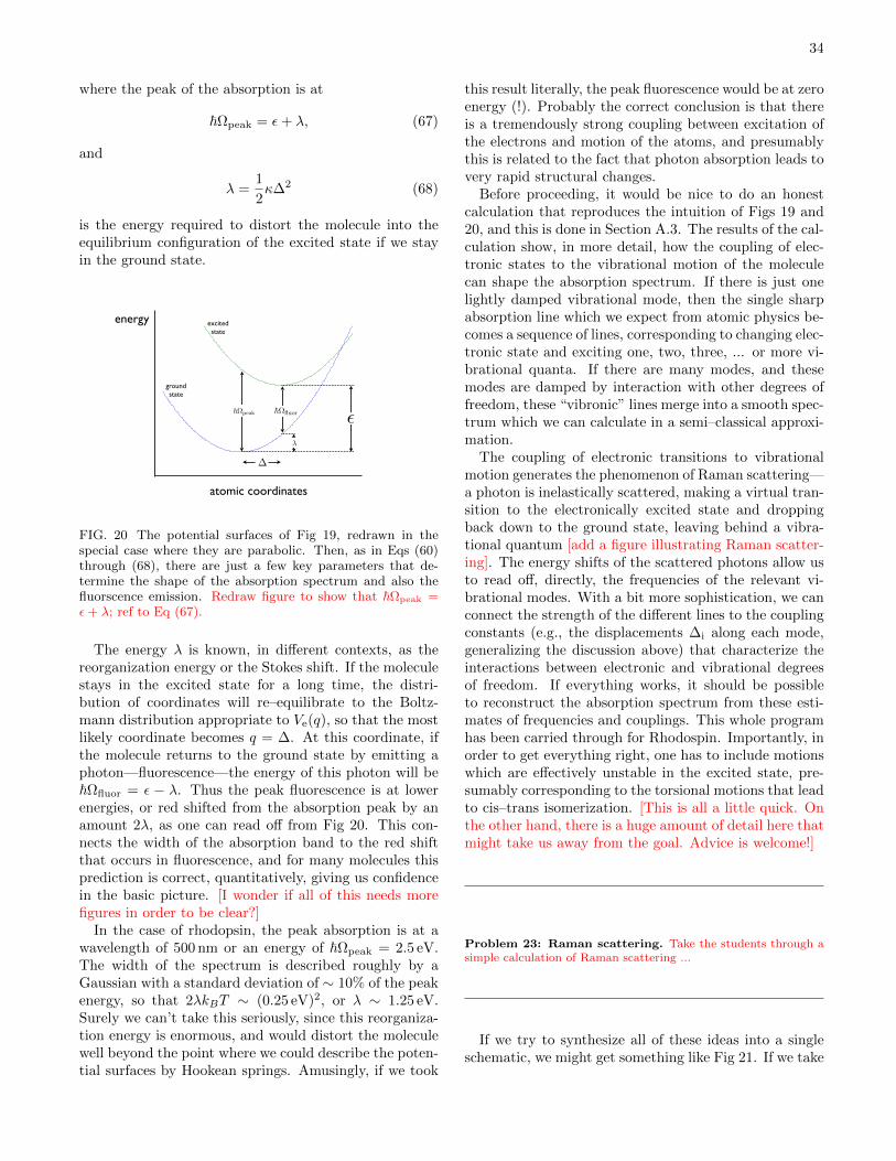
34

where the peak of the absorption is at

!$peak = ,+ *, (67)

and

* =1

2+#2 (68)

is the energy required to distort the molecule into theequilibrium configuration of the excited state if we stayin the ground state.

!! !"#$ !" !%#$ % %#$ " "#$ ! !#$ &!!

%

!

'

(

)

"%energy

atomic coordinates

1.2. SINGLE MOLECULE DYNAMICS 35

a broadening of the absorption line.Concretely, if we imagine that the potential surfaces are perfect Hookean

springs, but with displaced equilibrium positions, then we can relate thewidth of the spectrum directly to the magnitude of this displacement. Inthe ground state we have the potential

V!(q) =1

2!q2, (1.50)

and in the excited state we have

V"(q) = "+1

2!(q !!)2, (1.51)

where " is the minimum energy di"erence between the two electronic statesand ! is the shift in the equilibrium position. With q fixed, the condition forabsorbing a photon is that the energy !# match the di"erence in electronicenergies,

!# = V"(q)! V!(q) = "+1

2!!2 ! !!q. (1.52)

The probability distribution of q when molecules are in the ground state isgiven by

P (q) " exp

!!V!(q)

kBT

"= exp

!! !q2

2kBT

", (1.53)

so we expect the absorption cross–section to have the form

#(#) ##

dq P (q)$

!!#!

$"+

1

2!!2 ! !!q

%"(1.54)

"#

dq exp

!! !q2

2kBT

"$

!!#!

$"+

1

2!!2 ! !!q

%"(1.55)

" exp

!!(!#! !#peak)2

4%kBT

", (1.56)

where the peak of the absorption is at

!#peak = "+ %, (1.57)

and

% =1

2!!2 (1.58)

is the energy required to distort the molecule into the equilibrium configu-ration of the excited state if we stay in the ground state.

1.2. SINGLE MOLECULE DYNAMICS 35

a broadening of the absorption line.Concretely, if we imagine that the potential surfaces are perfect Hookean

springs, but with displaced equilibrium positions, then we can relate thewidth of the spectrum directly to the magnitude of this displacement. Inthe ground state we have the potential

V!(q) =1

2!q2, (1.50)

and in the excited state we have

V"(q) = "+1

2!(q !!)2, (1.51)

where " is the minimum energy di"erence between the two electronic statesand ! is the shift in the equilibrium position. With q fixed, the condition forabsorbing a photon is that the energy !# match the di"erence in electronicenergies,

!# = V"(q)! V!(q) = "+1

2!!2 ! !!q. (1.52)

The probability distribution of q when molecules are in the ground state isgiven by

P (q) " exp

!!V!(q)

kBT

"= exp

!! !q2

2kBT

", (1.53)

so we expect the absorption cross–section to have the form

#(#) ##

dq P (q)$

!!#!

$"+

1

2!!2 ! !!q

%"(1.54)

"#

dq exp

!! !q2

2kBT

"$

!!#!

$"+

1

2!!2 ! !!q

%"(1.55)

" exp

!!(!#! !#peak)2

4%kBT

", (1.56)

where the peak of the absorption is at

!#peak = "+ %, (1.57)

and

% =1

2!!2 (1.58)

is the energy required to distort the molecule into the equilibrium configu-ration of the excited state if we stay in the ground state.

1.2. SINGLE MOLECULE DYNAMICS 35

a broadening of the absorption line.Concretely, if we imagine that the potential surfaces are perfect Hookean

springs, but with displaced equilibrium positions, then we can relate thewidth of the spectrum directly to the magnitude of this displacement. Inthe ground state we have the potential

V!(q) =1

2!q2, (1.50)

and in the excited state we have

V"(q) = "+1

2!(q !!)2, (1.51)

where " is the minimum energy di"erence between the two electronic statesand ! is the shift in the equilibrium position. With q fixed, the condition forabsorbing a photon is that the energy !# match the di"erence in electronicenergies,

!# = V"(q)! V!(q) = "+1

2!!2 ! !!q. (1.52)

The probability distribution of q when molecules are in the ground state isgiven by

P (q) " exp

!!V!(q)

kBT

"= exp

!! !q2

2kBT

", (1.53)

so we expect the absorption cross–section to have the form

#(#) ##

dq P (q)$

!!#!

$"+

1

2!!2 ! !!q

%"(1.54)

"#

dq exp

!! !q2

2kBT

"$

!!#!

$"+

1

2!!2 ! !!q

%"(1.55)

" exp

!!(!#! !#peak)2

4%kBT

", (1.56)

where the peak of the absorption is at

!#peak = "+ %, (1.57)

and

% =1

2!!2 (1.58)

is the energy required to distort the molecule into the equilibrium configu-ration of the excited state if we stay in the ground state.

groundstate

excitedstate

36 CHAPTER 1. PHOTON COUNTING IN VISION

The energy ! is known, in di!erent contexts, as the reorganization energyor the Stokes shift. If the molecule stays in the excited for a long time, weexpect that the distribution of coordinates will re–equilibrate to the Boltz-mann distribution appropriate to V!(q), so that the most likely coordinatebecomes q = ". At this coordinate, if the molecule returns to the groundstate by emitting a photon—fluorescence—the energy of this photon will be!#fluor = "!! Thus the peak fluorescence is red shifted from the absorptionpeak by 2!. This connects the width of the absorption band to the redshift that occurs in fluorescence, and for many molecules this prediction iscorrect, quantitatively, giving us confidence in the basic picture.

finish thisIt would be nice to do an honest calculation that reproduces the intuition

of Fig 1.12. We have a system with two electronic states, which we canrepresent as a spin one–half; let spin down be the ground state and spin upbe the excited state. The Born–Oppenheimer approximation tells us thatprobably will mention

B–O above; be sure toconnect

we can think of the atoms in a molecule as moving in a potential determinedby the electronic state, which we denote by V!(q) and V"(q) in the excitedand ground states, respectively; q stands for all the atomic coordinates.Since we are observing photon absorption, there must be a matrix elementthat connects the two electronic states and couples to the electromagneticfield; we’ll assume that, absent symmetries, this coupling is dominated by anelectric dipole term. In principle the dipole matrix element #d could dependupon the atomic coordinates, but we’ll neglect this e!ect.4 Putting the piecetogether, we have the Hamiltonian for the molecule

H = K+1

2(1 + $z)V!(q) +

1

2(1! $z)V"(q) + #d· #E($+ + $#), (1.59)

where K is the kinetic energy of the atoms. To this we should of course addthe usual Hamiltonian for the electromagnetic field.

We are interested in computing the rate at which photons of energy !#are absorbed, and of course we will do this as a perturbation expansion inthe term " #d. The result of such a calculation can be presented as the‘Golden rule’ for transition rates, but this formulation hides the underlyingdynamics. So, at the risk of being pedantic, I’ll go through the steps thatusually lead to the Golden rule and take a detour that leads us to a formulain which the dynamics of atomic motions are more explicit.5

4In practice, this is a small e!ect. You should think about why this is true.5I am assuming something about the background of my students—that the Golden rule

is well known, but that the general tools which relate cross–sections and transition ratesto correlation functions are less well digested.

1.2. SINGLE MOLECULE DYNAMICS 35

a broadening of the absorption line.Concretely, if we imagine that the potential surfaces are perfect Hookean

springs, but with displaced equilibrium positions, then we can relate thewidth of the spectrum directly to the magnitude of this displacement. Inthe ground state we have the potential

V!(q) =1

2!q2, (1.50)

and in the excited state we have

V"(q) = "+1

2!(q !!)2, (1.51)

where " is the minimum energy di"erence between the two electronic statesand ! is the shift in the equilibrium position. With q fixed, the condition forabsorbing a photon is that the energy !# match the di"erence in electronicenergies,

!# = V"(q)! V!(q) = "+1

2!!2 ! !!q. (1.52)

The probability distribution of q when molecules are in the ground state isgiven by

P (q) " exp

!!V!(q)

kBT

"= exp

!! !q2

2kBT

", (1.53)

so we expect the absorption cross–section to have the form

#(#) ##

dq P (q)$

!!#!

$"+

1

2!!2 ! !!q

%"(1.54)

"#

dq exp

!! !q2

2kBT

"$

!!#!

$"+

1

2!!2 ! !!q

%"(1.55)

" exp

!!(!#! !#peak)2

4%kBT

", (1.56)

where the peak of the absorption is at

!#peak = "+ %, (1.57)

and

% =1

2!!2 (1.58)

is the energy required to distort the molecule into the equilibrium configu-ration of the excited state if we stay in the ground state.

FIG. 20 The potential surfaces of Fig 19, redrawn in thespecial case where they are parabolic. Then, as in Eqs (60)through (68), there are just a few key parameters that de-termine the shape of the absorption spectrum and also thefluorscence emission. Redraw figure to show that !#peak ='+ $; ref to Eq (67).

The energy * is known, in di!erent contexts, as thereorganization energy or the Stokes shift. If the moleculestays in the excited state for a long time, the distri-bution of coordinates will re–equilibrate to the Boltz-mann distribution appropriate to Ve(q), so that the mostlikely coordinate becomes q = #. At this coordinate, ifthe molecule returns to the ground state by emitting aphoton—fluorescence—the energy of this photon will be!$fluor = , " *. Thus the peak fluorescence is at lowerenergies, or red shifted from the absorption peak by anamount 2*, as one can read o! from Fig 20. This con-nects the width of the absorption band to the red shiftthat occurs in fluorescence, and for many molecules thisprediction is correct, quantitatively, giving us confidencein the basic picture. [I wonder if all of this needs morefigures in order to be clear?]

In the case of rhodopsin, the peak absorption is at awavelength of 500 nm or an energy of !$peak = 2.5 eV.The width of the spectrum is described roughly by aGaussian with a standard deviation of ! 10% of the peakenergy, so that 2*kBT ! (0.25 eV)2, or * ! 1.25 eV.Surely we can’t take this seriously, since this reorganiza-tion energy is enormous, and would distort the moleculewell beyond the point where we could describe the poten-tial surfaces by Hookean springs. Amusingly, if we took

this result literally, the peak fluorescence would be at zeroenergy (!). Probably the correct conclusion is that thereis a tremendously strong coupling between excitation ofthe electrons and motion of the atoms, and presumablythis is related to the fact that photon absorption leads tovery rapid structural changes.Before proceeding, it would be nice to do an honest

calculation that reproduces the intuition of Figs 19 and20, and this is done in Section A.3. The results of the cal-culation show, in more detail, how the coupling of elec-tronic states to the vibrational motion of the moleculecan shape the absorption spectrum. If there is just onelightly damped vibrational mode, then the single sharpabsorption line which we expect from atomic physics be-comes a sequence of lines, corresponding to changing elec-tronic state and exciting one, two, three, ... or more vi-brational quanta. If there are many modes, and thesemodes are damped by interaction with other degrees offreedom, these “vibronic” lines merge into a smooth spec-trum which we can calculate in a semi–classical approxi-mation.The coupling of electronic transitions to vibrational

motion generates the phenomenon of Raman scattering—a photon is inelastically scattered, making a virtual tran-sition to the electronically excited state and droppingback down to the ground state, leaving behind a vibra-tional quantum [add a figure illustrating Raman scatter-ing]. The energy shifts of the scattered photons allow usto read o!, directly, the frequencies of the relevant vi-brational modes. With a bit more sophistication, we canconnect the strength of the di!erent lines to the couplingconstants (e.g., the displacements #i along each mode,generalizing the discussion above) that characterize theinteractions between electronic and vibrational degreesof freedom. If everything works, it should be possibleto reconstruct the absorption spectrum from these esti-mates of frequencies and couplings. This whole programhas been carried through for Rhodospin. Importantly, inorder to get everything right, one has to include motionswhich are e!ectively unstable in the excited state, pre-sumably corresponding to the torsional motions that leadto cis–trans isomerization. [This is all a little quick. Onthe other hand, there is a huge amount of detail here thatmight take us away from the goal. Advice is welcome!]

Problem 23: Raman scattering. Take the students through asimple calculation of Raman scattering ...

If we try to synthesize all of these ideas into a singleschematic, we might get something like Fig 21. If we take

35

FIG. 21 Schematic model of the energy surfaces inRhodopsin. The ground state has minima at both the 11–cis and the all–trans structures. A single excited state sitsabove this surface. At some intermediate structure, the sur-faces come very close. At this point, the Born–Oppenheimerapproximation breaks down, and there will be some mixingbetween the two states. A molecule lifted into the excitedstate by absorbing a photon slides down the upper surface,and can pass non–adiabatically into the potential well whoseminimum is at all–trans.

this picture seriously, then after exciting the moleculewith a pulse of light, we should see the disappearanceof the absorption band associated with the 11–cis struc-ture, the gradual appearance of the absorption from theall–trans state, and with a little luck, stimulated emis-sion while the excited state is occupied. All of this isseen. Looking closely (e.g., at Fig 17), however, one seesthat spectra are oscillating in time. Rather than slid-ing irreversibly down the potential surfaces toward theirminima, the atomic structure oscillates. More remark-ably, detailed analysis of the time evolution of the spectrademonstrates that there is coherent quantum mechani-cal mixing among the relevant electronic and vibrationalstates.

Our usual picture of molecules and their transitionscomes from chemical kinetics: there are reaction rates,which represent the probability per unit time for themolecule to make transitions among states which are dis-tinguishable by some large scale rearrangement; thesetransitions are cleanly separated from the time scales formolecules to come to equilibrium in each state. The ini-tial isomerization event in rhodopsin is so fast that thisapproximation certainly breaks down. More profoundly,the time scale of the isomerization is so fast that it com-petes with the processes that destroy quantum mechan-ical coherence among the relevant electronic and vibra-tional states. The whole notion of an irreversible tran-sition from one state to another necessitates the loss ofcoherence between these states (recall Schrodinger’s cat),

and so in this sense the isomerization is proceeding asrapidly as possible.At this point what we would like to do is an honest,

if simplified calculation that generates the schematic inFig 21 and explains how the dynamics on these surfacescan be so fast. As far as I know, there is no clear answerto this challenge, although there are many detailed sim-ulations, in the quantum chemical style, that probablycapture elements of the truth.[it would be nice to be alittle more explicit here!] The central ingredient is thespecial nature of the $ bonds along the retinal. In theground state, electron hopping between neighboring pzorbitals lowers the energy of the system, and this e!ect ismaximized in planar structures where the orbitals are allin the same orientation. But this lowering of the energydepends on the character of the electron wave functions—in the simplest case of bonding between two atoms, thesymmetric state (the ‘bonding orbital’) has lower energyin proportion to the hopping matrix element, while theanti–symmetric state (‘anti–bonding orbital’) has higherenergy, again in proportion to the matrix element. Thus,if we excite the electrons, it is plausible that the energy ofthe excited state could be reduced by structural changesthat reduce the hopping between neighboring carbons,which happens if the molecule rotates to become non–planar. In this way we can understand why there is aforce for rotation in the excited state, and why there isanother local minimum in the ground state at the 11–cisstructure.

Problem 24: Energy levels in conjugated molecules. Thesimplest model for a conjugated molecule is that the electrons whichform the & orbitals can sit on each carbon atom with some energythat we can set to zero, and they can hop from one atom to itsneighbors. Note that there is one relevant electron per carbonatom. If we write the Hamiltonian for the electrons as a matrix,then for a ring of six carbons (benzene) we have

H6 =

(

)))))*

0 !t 0 0 0 !t!t 0 !t 0 0 00 !t 0 !t 0 00 0 !t 0 !t 00 0 0 !t 0 !t!t 0 0 0 !t 0

+

,,,,,-, (69)

where the “hopping matrix element” !t is negative because theelectrons can lower their energy by being shared among neighboringatoms—this is the essence of chemical bonding! Models like thisare called tight binding models in the condensed matter physicsliterature and Huckel models in the chemical literature. Noticethat they leave out any direct interactions among the electrons.This problem is about solving Schrodinger’s equation, H$ = E$,to find the energy eigenstates and the corresponding energy levels.Notice that for the case of benzene if we write the wave function$ in terms of its six components (one for each carbon atom) then

36

Schrodinger’s equation becomes

!t($2 + $6) = E$1 (70)

!t($1 + $3) = E$2 (71)

!t($2 + $4) = E$3 (72)

!t($3 + $5) = E$4 (73)

!t($4 + $6) = E$5 (74)

!t($5 + $1) = E$6. (75)

(a.) Considering first the case of benzene, show that solutionsto the Schrodinger equation are of the form $n + exp(ikn). Whatare the allowed values of the “momentum” k? Generalize to anarbitrary N–membered ring.

(b.) What are the energies corresponding to the states labeled byk? Because of the Pauli principle, the ground state of the molecule

is constructed by putting the electrons two–by–two (spin up andspin down) into the lowest energy states; thus the ground state ofbenzene has two electrons in each of the lowest three states. Whatis the ground state energy of benzene? What about for an arbitraryN–membered ring (with N even)? Can you explain why benzeneis especially stable?

(c.) Suppose that the bonds between carbon atoms stretch andcompress a bit, so that they become alternating single and doublebonds rather than all being equivalent. To first order, if the bondstretches by an amount u then the hopping matrix element shouldgo down (the electron has farther to hop), so we write t $ t !#u; conversely, if the bond compresses, so that u is negative, thehopping matrix element gets larger. If we have alternating longand short (single and double) bonds, then the Hamiltonian for ansix membered ring would be

H6(u) =

(

)))))*

0 !t+ #u 0 0 0 !t! #u!t+ #u 0 !t! #u 0 0 0

0 !t! #u 0 !t+ #u 0 00 0 !t+ #u 0 !t! #u 00 0 0 !t! #u 0 !t+ #u

!t! #u 0 0 0 !t+ #u 0

+

,,,,,-.

(76)

Find the ground state energy of the electrons as a function of u,and generalize to the case of N–membered rings. Does the “dimer-ization” of the system (u -= 0) raise or lower the energy of theelectrons? Note that if your analytic skills (or patience!) give out,this is a relatively simple numerical problem; feel free to use thecomputer, but be careful to explain what units you are using whenyou plot your results.

(d.) In order to have bonds alternately stretched and compressedby an amount u, we need an energy 1

2*u2 in each bond, where *

is the sti!ness contributed by all the other electrons that we’re notkeeping track of explicitly. Consider parameter values t = 2.5 eV,

# = 4.1 eV/A, and * = 21 eV/A2. Should benzene have alternating

single and double bonds (u -= 0) or should all bonds be equivalent(u = 0)?

(e.) Peierls’ theorem about one–dimensional electron systemspredicts that, for N–carbon rings with N large, the minimum totalenergy will be at some non–zero u#. Verify that this is true in thiscase, and estimate u#. How large does N have to be before it’s“large”? What do you expect for retinal?

I could try to do a full calculation here that puts fleshon the outline in the previous paragraph, using the toolsfrom the problem above. But there still is a problem evenif this works ...

Suppose that we succeed, and have a semi–quantitativetheory of the excited state dynamics of rhodopsin,enough to understand why the quantum yield of fluo-rescence is so low, and what role is played by quantumcoherence. We would then have to check that the barrierbetween the 11–cis and the all–trans structures in Fig 21comes out to have the right height to explain the acti-vation energy for spontaneous isomerization. But thenhow do we account for the anomalously low prefactor in

this rate, which is where, as discussed above, the proteinacts to suppress dark noise? If there is something specialabout the situation in the environment of the proteinwhich makes possible the ultrafast, coherent dynamicsin the excited state, why does this special environmentgenerate almost the same barrier as for isolated retinal?It is clear that the ingredients for understanding the

dynamics of rhodopsin—and hence for understandingwhy we can see into the darkest times of night—involvequantum mechanical ideas more related to condensedmatter physics than to conventional biochemistry, a re-markably long distance from the psychology experimentson human subjects that we started with. While Lorentzcould imagine that people count single quanta, surely hecouldn’t have imagined that he first steps of this processare coherent. While these are the ingredients, it is clearthat we don’t have them put together in quite the rightway yet.If rhodopsin were the only example of this “almost co-

herent chemistry” that would be good enough, but in factthe other large class of photon induced events in biologi-cal systems—photosynthesis—also proceed so rapidly asto compete with loss of coherence, and the crucial eventsagain seem to happen (if you’ll pardon the partisanship)while everything is still in the domain of physics and notconventional chemistry. Again there are beautiful exper-iments that present a number of theoretical challenges.20

20 As usual, a guide is found in the references at the end of thissection.

37

Why biology pushes to these extremes is a good question.How it manages to do all this with big floppy moleculesin water at roughly room temperature also is a greatquestion.

To get some of the early history of work on the visual pigments,one can do worse than to read Wald’s Nobel lecture (Wald 1972).Wald himself (along with his wife and collaborator, Ruth Hubbard)was quite an interesting fellow, much involved in politics; to con-nect with the previous section, his PhD adviser was Selig Hecht.[need more about dark noise and temperature dependence?] For ameasurement of dark noise in cones, see Sampath & Baylor (2002).The remarkable result that the quantum yield of fluorescence inrhodopsin is # 10"5 is due to Doukas et al (1984); it’s worth not-ing that measuring this small quantum yield was possible at a timewhen one could not directly observe the ultrafast processes thatare responsible for making the branching ratio this small. Directmeasurements were finally made by Mathies et al (1988), Schoen-lein et al (1991), and Wang et al (1994), the last paper makingclear that the initial events are quantum mechanically coherent. Adetailed analysis of the Raman spectra of Rhodopsin has been doneby Loppnow & Mathies (1988).

Doukas et al 1984: Fluorescence quantum yield of visual pig-ments: Evidence for subpicosecond isomerization rates. AGDoukas, MR Junnarkar, RR Alfano, RH Callender, T Kak-itani & B Honig, Proc Nat Acad Sci (USA) 81, 4790–4794(1984).

Loppnow & Mathies 1988: Excited-state structure and isomer-ization dynamics of the retinal chromophore in rhodopsinfrom resonance Raman intensities GR Loppnow & RAMath-ies, Biophys J 54, 35–43 (1988).

Mathies et al 1988: Direct observation of the femtosecondexcited–state cis–trans isomerization in bacteriorhodopsin.RA Mathies, CH Brito Cruz, WT Pollard & CV Shank,Science 240, 777–779 (1988).

Sampath & Baylor 2002: Molecular mechanisms of sponta-neous pigment activation in retinal cones. AP Sampath &DA Baylor, Biophys J 83, 184–193 (2002).

Schoenlein et al 1991: The first step in vision: Femtosecondisomerization of rhodopsin. RW Schoenlein, LA Peteanu,RA Mathies & CV Shank, Science 254, 412–415 (1991).

Wald 1972: The molecular basis of visual excitation. GWald, in Nobel Lectures: Physiology or Medicine 1963–1970 (Elsevier, Amsterdam, 1972). Also available athttp://nobelprize.org.

Wang et al 1994: Vibrationally coherent photochemistry in thefemtosecond primary event of vision. Q Wang, RW Schoen-lein, LA Peteanu, RA Mathies & CV Shank, Science 266,422–424 (1994).

The Born–Oppenheimer approximation is discussed in almost allquantum mechanics textbooks. For a collection of the key papers,with commentary, on the rich phenomena that can emerge in suchadiabatic approximations, see Shapere & Wilczek (1989). Modelsfor coupling of electron hopping to bond stretching (as in the lastproblem) were explored by Su, Schrie!er and Heeger in relationto polyacetylene. Importantly, these models predict that the exci-tations (e.g., upon photon absorption) are not just electrons andholes in the usual ladder of molecular orbitals, but that there arelocalized, mobile objects with unusual quantum numbers. Thesemobile objects can be generated by doping, which is the basis forconductivity in these quasi–one dimensional materials. The origi-nal work in Su et al (1980); a good review is Heeger et al (1988).Many people must have realized that the dynamical models beingused by condensed matter physicists for (ideally) infinite chains

might also have something to say about finite chains. For ideas inthis direction, including some specifically relevant to Rhodopsin,see Bialek et al (1987), Vos et al (1996), and Aalberts et al (2000).

Aalberts et al 2000: Quantum coherent dynamics of molecules:A simple scenario for ultrafast photoisomerization. DP Aal-berts, MSL du Croo de Jongh, BF Gerke & W van Saarloos,Phys Rev A 61, 040701 (2000).

Heeger et al 1988: Solitons in conducting polymers. AJ Heeger,S Kivelson, JR Schrie!er & W–P Su, Rev Mod Phys 60,781–850 (1988).

Bialek et al 1987: Simple models for the dynamics ofbiomolecules: How far can we go?. W Bialek, RFGoldstein & S Kivelson, in Structure, Dynamics andFunction of Biomolecules: The First EBSA Workshop, AEhrenberg, R Rigler, A Graslund & LJ Nilsson, eds, pp65–69 (Springer–Verlag, Berlin, 1987).

Shapere & Wilczek 1989: Geometric Phases in Physics AShapere and F Wilczek (World Scientific, Singapore, 1989)

Su et al 1980: Soliton excitations in polyacetylene. W–P Su, JRSchrie!er & AJ Heeger, Phys Rev B 22, 2099–2111 (1980).

Vos et al 1996: Su–Schrie!er–Heeger model applied to chains offinite length. FLJ Vos, DP Aalberts & W van Saarloos, PhysRev B 53, 14922–14928 (1996).

Going beyond the case of rhodopsin, you may want to explore therole of quantum coherence in the initial events of photosynthe-sis; for an introduction see Fleming & van Grondelle (1994). Thefirst experiments focused on photo–induced electron transfer, andlooked at systems that had been genetically modified so that theelectron, once excited, had no place to go (Vos et al 1991, Vos et al1993); this made it possible to see the coherent vibrational motionof the molecule more clearly in spectroscopic experiments. Sub-sequent experiments used more intact systems, but looked first atlow temperatures (Vos et al 1994a) and finally at room tempera-ture (Vos et al 1994b). Eventually it was even possible to show thatphoto–triggering of electron transfer in other systems could revealcoherent vibrational motions (Liebl et al 1999). More or less at thesame time as the original Vos et al experiments, my colleagues andI made the argument that photo–induced electron transfer ratesin the initial events of photosynthesis would be maximized if thesystem were poised on the threshold of revealing coherent e!ects;maybe (although there were uncertainties about all the parameters)one could even strengthen this argument to claim that the observedrates were possible only in this regime (Skourtis et al 1992). Mostrecently, it has been discovered that when energy is trapped inthe “antenna pigments” of photosynthetic systems, the migrationof energy toward the reaction center (where the electron transferoccurs) is coherent, and it has been suggested that this allows fora more e"cient exploration of space, finding the target faster thanis possible in di!usive motion (Engel et al 2007). [Decide what tosay about the large follow up literature!]

Engel et al 2007: Evidence for wavelike energy transfer throughquantum coherence in photosynthetic systems. GS En-gel, TR Calhoun, EL Read, T–K Ahn, T Mancal, Y–CChengm RE Blankenship & GR Fleming, Nature 446, 782–786 (2007).

Fleming & van Grondelle 1994: The primary steps of photo-synthesis. GR Fleming & R van Grondelle, Physics Todaypp 48–55, February 1994.

Liebl et al 1999: Coherent reaction dynamics in a bacterial cy-tochrome c oxidase. U Liebl, G Lipowski, M Negrerie, JCLambry, JL Martin & MH Vos, Nature 401, 181–184 (1999).

Skourtis et al 1992: A new look at the primary charge separa-tion in bacterial photosynthesis. SS Skourtis, AJR DaSilva,W Bialek & JN Onuchic, J Phys Chem 96, 8034–8041(1992).

Vos et al 1991: Direct observation of vibrational coherence inbacterial reaction centers using femtosecond absorption

38

spectroscopy. MH Vos, JC Lambry, SJ Robles, DC You-van, J Breton & JL Martin, Proc Nat’l Acad Sci (USA) 88,8885–8889 (1991).

Vos et al 1993: Visualization of coherent nuclear motion in amembrane protein by femtosecond spectroscopy. MH Vos,F Rappaport, JC Lambry, J Breton & JL Martin, Nature363, 320–325 (1993).

Vos et al 1994a: Coherent dynamics during the primary electrontransfer reaction in membrane–bound reaction centers ofRhodobacter sphaeroides. MH Vos, MR Jones, CN Hunter,J Breton, JC Lambry & JL Martin, Biochemistry 33, 6750–6757 (1994).

Vos et al 1994b: Coherent nuclear dynamics at room tempera-ture in bacterial reaction centers. MH Vos, MR Jones, CNHunter, J Breton, JC Lambry & JL Martin, Proc Nat’l AcadSci (USA) 91, 12701–12705 (1994).

C. Dynamics of biochemical networks

Section still needs editing, as of September 18, 2011.The material here seems to have accreted during theearly versions of the course, and much time is spent onthings which we now know aren’t productive ... . Onthe other hand, I would like to say more about, for ex-ample, Sengupta et al (2000) on SNR in cascades andgain–bandwidth, as well as returning to the problem oftransduction in invertebrates, e.g. theoretical work fromShraiman, Ranganathan et al.. So, I’d like make a morethorough overhaul here!

We have known for a long time that light is absorbedby rhodopsin, and that light absorption leads to an elec-trical response which is detectable as a modulation in thecurrent flowing across the photoreceptor cell membrane.It is only relatively recently that we have come to under-stand the mechanisms which link these two events. Thenature of the link is qualitatively di!erent in di!erentclasses of organisms. For vertebrates, including us, thesituation is as schematized in Fig 22. [it would be niceto come back and talk about invertebrates too]

In outline, what happens is that the excited rhodopsinchanges its structure, arriving after several steps in astate where it can act as a catalyst to change the struc-ture of another protein called transducin (T). The acti-vated transducin in turn activates a catalyst called phos-phodiesterase (PDE), which breaks down cyclic guano-sine monophospate (cGMP). Finally, cGMP binds tochannels in the cell membrane and opens the channels,allowing current to flow (mostly carried by Na+ ions);breaking down the cGMP thus decreases the number ofopen channels and decreases the current. [This discus-sion needs to refer to a schematic of the rod cell. Whereis this? Earlier? Here?]

In a photomultiplier, photon absorption results in theejection of a primary photoelectron, and then the large

Rh

Rh*

T

T*

PDE

PDE*

cGMP

GMP

GTPGC

output:open

channels

GTP

input:photon

absorption

FIG. 22 The cascade leading from photon absorption to ioniccurrent flow in rod photoreceptors. Solid lines indicate ‘for-ward’ steps that generate gain; dashed lines are the ‘back-ward’ steps that shut o! the process. T is the transducinmolecule, a member of the broad class of G–proteins thatcouple receptors to enzymes. PDE is the enzyme phospho-diesterase, named for the particular bond that it cuts whenit degrades cyclic guanosine monophosphate (cGMP) intoGMP. GC is the guanylate cyclase that synthesizes cGMPfrom guanosine triphosphate, GTP.

electric field accelerates this electron so that when it hitsthe next metal plate it ejects many electrons, and theprocess repeats until at the output the number of elec-trons is su"ciently large that it constitutes a macroscopiccurrent. Thus the photomultiplier really is an electronmultiplier. In the same way, the photoreceptor acts asa molecule multiplier, so that for one excited rhodopsinmolecule there are many cGMP molecules degraded atthe output of the “enzymatic cascade.”There are lots of interesting questions about how the

molecule multiplication actually works in rod photore-ceptors. These questions are made more interesting bythe fact that this general scheme is ubiquitous in biologi-cal systems. [need a schematic about G–protein coupledreceptors!] Rhodopsin is a member of a family of proteinswhich share common structural features (seven alpha he-lices that span the membrane in which the protein isembedded) and act as receptors, usually activated by thebinding of small molecules such as hormones or odorantsrather than light. Proteins in this family interact withproteins from another family, the G proteins, of whichtransducin is an example, and the result of such interac-tions typically is the activation of yet another enzyme, of-ten one which synthesizes or degrades a cyclic nucleotide.Cyclic nucleotides in turn are common intracellular mes-sengers, not just opening ion channels but also activatingor inhibiting a variety of enzymes. This universality ofcomponents means that understanding the mechanismsof photon counting in rod cells is not just a curiosity forphysicists, but a place where we can provide a model forunderstanding an enormous range of biological processes.

39

In order to get started, we need to know a little bitabout ion channels, which form the output of the system.We will see that even the simplest, order–of–magnitudeproperties of channels raise a question about the observedbehavior of the rod cells.Recall that the brain contains no metallic or semicon-

ductor components. Signals can still be carried by elec-trical currents and voltages, but now currents consist ofions, such as potassium or sodium, flowing through wateror through specialized conducting pores. These pores, orchannels, are large molecules (proteins) embedded in thecell membrane, and can thus respond to the electric fieldor voltage across the membrane as well as to the bindingof small molecules. The coupled dynamics of channelsand voltage turns each cell into a potentially complexnonlinear dynamical system.Imagine a spherical molecule or ion of radius a; a typi-

cal value for this radius is 0.3 nm. From Stokes’ formulawe know that if this ion moves through the water at ve-locity v it will experience a drag force F = -v, with thedrag coe"cient - = 6$.a, where . is the viscosity; forwater . = 0.01 poise, the cgs unit poise = gm/(cm · s).The inverse of the drag coe"cient is called the mobil-ity, µ = 1/-, and the di!usion constant of a particleis related to the mobility and the absolute tempera-ture by the Einstein relation or fluctuation dissipationtheorem, D = kBTµ, with kB being Boltzmann’s con-stant and T the absolute temperature. Since life oper-ates in a narrow range of absolute temperatures, it isuseful to remember that at room temperature (25$C),kBT ! 4 ( 10!21 J ! 1/40 eV. So let’s write the di!u-sion constant in terms of the other quantities, and thenevaluate the order of magnitude:

D = kBTµ = kBT · 1-=

kBT

6$.a(77)

=[4( 10!21 J]

6$ · [0.01 gm/(cm · s)] · [0.3( 10!9 m](78)

! 2( 10!9m2/ s = 2µm2/ms. (79)

Ions and small molecules di!use freely through water,but cells are surrounded by a membrane that functionsas a barrier to di!usion. In particular, these membranesare composed of lipids, which are nonpolar, and there-fore cannot screen the charge of an ion that tries to passthrough the membrane. The water, of course, is polarand does screen the charge, so pulling an ion out of thewater and pushing it through the membrane would re-quire surmounting a large electrostatic energy barrier.This barrier means that the membrane provides an enor-mous resistance to current flow between the inside andthe outside of the cell. If this were the whole story therewould be no electrical signaling in biology. In fact, cellsconstruct specific pores or channels through which ionscan pass, and by regulating the state of these channelsthe cell can control the flow of electric current across themembrane. [need a sketch that goes with this discussion]

Ion channels are themselves molecules, but very largeones—they are proteins composed of several thousandatoms in very complex arrangements. Let’s try, however,to ask a simple question: If we open a pore in the cellmembrane, how quickly can ions pass through? Moreprecisely, since the ions carry current and will move inresponse to a voltage di!erence across the membrane,how large is the current in response to a given voltage?Imagine that one ion channel serves, in e!ect, as a hole

in the membrane. Let us pretend that ion flow throughthis hole is essentially the same as through water. Theelectrical current that flows through the channel is

J = qion · [ionic flux] · [channel area], (80)

where qion is the charge on one ion, and we recall that‘flux’ measures the rate at which particles cross a unitarea, so that

ionic flux =ions

cm2s=

ions

cm3· cm

s(81)

= [ionic concentration] · [velocity of one ion]

= cv. (82)

Major current carriers such as sodium and potassiumare at concentrations of c ! 100 mM, or c ! 6 (1019 ions/cm3.The next problem is to compute the typical velocity of

one ion. We are interested in a current, so this is not thevelocity of random Brownian motion but rather the aver-age of that component of the velocity directed along theelectric field. In a viscous medium, the average velocityis related to the applied force through the mobility, orthe inverse of the drag coe"cient as above. The force onan ion is in turn equal to the electric field times the ioniccharge, and the electric field is (roughly) the voltage dif-ference V across the membrane divided by the thickness& of the membrane:

v = µF = µqionE ! µqionV

&=

D

kBTqion

V

&. (83)

Putting the various factors together we find the current

J = qion · [ionic flux] · [channel area]= qion · [cv] · [$d2/4] (84)

= qion ·#c · D

&· qionVkBT

$· $d

2

4(85)

=$

4qion · cd

2D

&· qionVkBT

, (86)

where the channel has a diameter d. If we assume thatthe ion carries one electronic charge, as does sodium,potassium, or chloride, then qion = 1.6 ( 10!19 C andqionV /(kBT ) = V/(25 mV). Typical values for the chan-nel diameter should be comparable to the diameter of asingle ion, d ! 0.3 nm, and the thickness of the mem-brane is & ! 5 nm. Thus

40

J =$

4qion · cd

2D

&· qionVkBT

=$

4(1.6( 10!19 C) · (6( 1019 cm!3)(3( 10!8 cm)2(10!5 cm2/s)

50( 10!8 cm· V

25 mV(87)

! 2( 10!14 · V

mVC/s ! 2( 10!11 V

VoltsAmperes, (88)

or

J = gV (89)

g ! 2( 10!11 Amperes/Volt = 20 picoSiemens.(90)

So our order of magnitude argument leads us to pre-dict that the conductance of an open channel is roughly20 pS.21 With a voltage di!erence across the membraneof ! 50mV, we thus expect that opening a single channelwill cause ! 1 picoAmp of current to flow. Although in-credibly oversimplified, this is basically the right answer,as verified in experiments where one actually measuresthe currents flowing through single channel molecules.

The first problem in understanding the enzymatic cas-cade in rods is accessible just from these back of the en-velope arguments. When we look at the total changein current that results from a single photon arrival, itis also ! 1 pA. But if this were just the e!ect of (clos-ing) one channel, we’d see “square edges” in the currenttrace as the single channels opened or closed. It wouldalso be a little weird to have sophisticated (and expen-sive!) mechanisms for generating macroscopic changesin cGMP concentration only to have this act once againon a single molecule—if we have a single molecule inputand a single molecule output, it really isn’t clear why wewould need an amplifier. What’s going on?

The answer turns out to be that these channels flickervery rapidly between their open and closed states, so thaton the relatively slow time scale of the rod response onesees essentially a graded current proportional to the prob-ability of the channel being open. Thus the populationof channels in the rod cell membrane produces a cur-rent that depends continuously on the concentration ofcGMP. Alternatively, the noise variance that is associ-ated with the random binary variable open/closed hasbeen spread over a very broad bandwidth, so that in thefrequency range of interest (recall that the single photonresponse is on a time scale of ! 1 s) the noise is muchreduced. This idea is made precise in the following prob-lem, which you can think of as an introduction to the

21 Siemens are the units of conductance, which are inverse to unitsof resistance, ohms. In the old days, this inverse of resistance hadthe rather cute unit ‘mho’ (pronounced ‘moe,’ like the Stooge).

analysis of noise in “chemical” systems where moleculesfluctuate among multiple states.

Problem 25: Flickering channels. Imagine a channel thathas two states, open and closed. There is a rate kopen at which themolecule makes transitions from the closed state to the open state,and conversely there is a rate kclose at which the open channelstransition into the closed state. If we write the number of openchannels as nopen, and similarly for the number of closed channels,this means that the deterministic kinetic equations are

dnopen

dt= kopennclosed ! kclosenopen (91)

dnclose

dt= kclosenopen ! kopennclose, (92)

or, since nopen + nclosed = N , the total number of channels,

dnopen

dt= kopen(N ! nopen)! kclosenopen (93)

= !(kopen + kclose)nopen + kopenN. (94)

For a single channel molecule, these kinetic equations should beinterpreted as saying that an open channel has a probability kclosedtof making a transition to the closed state within a small time dt,and conversely a closed channel has a probability kopendt of makinga transition to the open state. We will give a fuller account of noisein chemical systems in the next Chapter, but for now you shouldexplore this simplest of examples.

(a.) If we have a finite number of channels, then really thenumber of channels which make the transition from the closed stateto the open state in a small window dt is a random number. Whatis the mean number of these closed $ open transitions? What isthe mean number of open $ closed transitions? Use your resultsto show that macroscopic kinetic equations such as Eqs (91) and(92) should be understood as equations for the mean numbers ofopen and closed channels,

d)nopen&dt

= kopen)nclosed& ! kclose)nopen& (95)

d)nclose&dt

= kclose)nopen& ! kopen)nclose&. (96)

(b.) Assuming that all the channels make their transitions in-dependently, what is the variance in the number of closed $ opentransitions in the small window dt? In the number of open $ closedtransitions? Are these fluctuations in the number of transitions in-dependent of one another?

(c.) Show that your results in [b] can be summarized by sayingthat the change in the number of open channels during the time dtobeys an equation

nopen(t+dt)!nopen(t) = dt[kopennclosed!kclosenopen]+,(t), (97)

where ,(t) is a random number that has zero mean and a variance

),2(t)& = dt[kopennclosed + kclosenopen]. (98)

41

Explain why the values of ,(t) and ,(t$) are independent if t -= t$.(d.) This discussion should remind you of the description of

Brownian motion by a Langevin equation, in which the determin-istic dynamics are supplemented by a random force that describesmolecular collisions. In this spirit, show that, in the limit dt $ 0,you can rewrite your results in [c] to give a Langevin equation forthe number of open channels,

dnopen

dt= !(kopen + kclose)nopen + kopenN + -(t), (99)

where

)-(t)-(t$)& = ((t! t$)[kopennclosed + kclosenopen]. (100)

In particular, if the noise is small, show that nopen = )nopen& +(nopen, where

d(nopen

dt= !(kopen + kclose)(nopen + -s(t), (101)

)-s(t)-s(t$)& = 2kopen)nclosed&. (102)

(e.) Solve Eq (101) to show that

)(n2open& = Npopen(1! popen) (103)

)(nopen(t)(nopen(t$)& = )(n2

open& exp.!|t! t$|

!c

/, (104)

where the probability of a channel being open is popen =kopen/(kopen + kclose), and the correlation time !c = 1/(kopen +kclose). Explain how the result for the variance )(n2

open& could bederived more directly.

(f.) Give a critical discussion of the approximations involved inwriting down these Langevin equations. In particular, in the caseof Brownian motion of a particle subject to ordinary viscous drag,the Langevin force has a Gaussian distribution. Is that true here?

Problem 26: Averaging out the noise. Consider a randomvariable such as nopen in the previous problem, for which the noisehas exponentially decaying correlations, as in Eq (104). Imaginethat we average over a window of duration !avg, to form a newvariable

z(t) =1

!avg

0 !avg

0d! (nopen(t! !). (105)

Show that, for !avg " !c, the variance of z is smaller than thevariance of (nopen by a factor of !avg/!c. Give some intuition forwhy this is true (e.g., how many statistically independent samplesof nopen will you see during the averaging time?). What happensif your averaging time is shorter?

I think this is a fascinating example, because evolutionhas selected for very fast channels to be present in a cellthat signals very slowly! Our genome (as well as those ofmany other animals) codes for hundreds if not thousandsof di!erent types of channels once one includes the pos-sibility of alternative splicing. These di!erent channelsdi!er, among other things, in their kinetics. In the flyretina, for example, the dynamics of visual inputs look-ing straight ahead are very di!erent from those looking tothe side, and in fact the receptor cells that look in thesedi!erent directions have di!erent kinds of channels—thefaster channels to respond to the more rapidly varyingsignals. [I am not sure that the last statement is correct,and need to check the references; what certainly is trueis that insects with di!erent lifestyles (e.g., acrobats vs.slow fliers) use di!erent potassium channels ... ] In the

FIG. 23 Current through the rod cell membrane as a functionof the cyclic GMP concentration. The fit is to Eq (106), withn = 2.9 ± 0.1 and G1/2 = 45 ± 4µM. From Rieke & Baylor(1996).

vertebrate rod, signals are very slow but the channels arefast, and this makes sense only if the goal is to suppressthe noise.Having understood a bit about the channels, let’s take

one step back and see how these channels respond tocyclic GMP. Experimentally, with the rod outer segmentsucked into the pipette for measuring current, one canbreak o! the bottom of the cell and make contact withits interior, so that concentrations of small molecules in-side the cell will equilibrate with concentrations in thesurrounding solution. Since the cell makes cGMP fromGTP, if we remove GTP from the solution then there isno source other than the one that we provide, and now wecan map current vs concentration. The results of such anexperiment are shown in Fig 23. We see that the currentI depends on the cGMP concentration G as

I = ImaxGn

Gn +Gn1/2

, (106)

with n + 3. This suggests strongly that the channelopens when three molecules of cGMP bind to it. Thisis an example of “cooperativity” or “allostery,” whichis a very important theme in biochemical signaling andregulation. It’s a little o! to the side of our discussionhere, however, so see Appendix A.4.Let’s try to write a more explicit model for the dynam-

ics of amplification in the rod cell, working back from thechannels. We have Eq (106), which tells us how the cur-rent I depends on G, the concentration of cyclic GMP.The dynamics of G has two terms, synthesis and degra-dation:

dG

dt= - " PDE#G, (107)

where - denotes the rate of synthesis by the guanylatecyclase (GC, cf Fig 22), and PDE# measures the activityof the active phosphodiesterase. It turns out that there

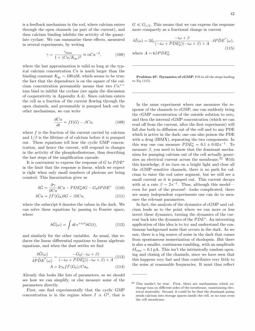
42

is a feedback mechanism in the rod, where calcium entersthrough the open channels (as part of the current), andthen calcium binding inhibits the activity of the guany-late cyclase. We can summarize these e!ects, measuredin several experiments, by writing

- =-max

1 + (Ca/Kgc)2+ "Ca!2, (108)

where the last approximation is valid so long at the typ-ical calcium concentration Ca is much larger than thebinding constant Kgc ! 100 nM, which seems to be true;the fact that the dependence is on the square of the cal-cium concentration presumably means that two Ca++

ions bind to inhibit the cyclase (see again the discussionof cooperativity in Appendix A.4). Since calcium entersthe cell as a fraction of the current flowing through theopen channels, and presumably is pumped back out byother mechanisms, we can write

dCa

dt= fI(G)" /Ca, (109)

where f is the fraction of the current carried by calciumand 1// is the lifetime of of calcium before it is pumpedout. These equations tell how the cyclic GMP concen-tration, and hence the current, will respond to changesin the activity of the phosphodiesterase, thus describingthe last steps of the amplification cascade.

It is convenient to express the response of G to PDE#

in the limit that the response is linear, which we expectis right when only small numbers of photons are beingcounted. This linearization gives us

(G =0-

0Ca(Ca" PDE#

0(G"G0(PDE# (110)

(Ca = fI %(G0)(G" /(Ca, (111)

where the subscript 0 denotes the values in the dark. Wecan solve these equations by passing to Fourier space,where

(G(!) =

%dt e+i#t(G(t), (112)

and similarly for the other variables. As usual, this re-duces the linear di!erential equations to linear algebraicequations, and when the dust settles we find

(G(!)

( ˜PDE#(!)

="G0("i! + /)

("i! + PDE#0 )("i! + /) +A

, (113)

A = 2-0fI%(G0)/Ca0. (114)

Already this looks like lots of parameters, so we shouldsee how we can simplify, or else measure some of theparameters directly.

First, one find experimentally that the cyclic GMPconcentration is in the regime where I * G3, that is

G , G1/2. This means that we can express the responsemore compactly as a fractional change in current

(I(!) = 3I0"i! + /

("i! + PDE#0 )("i! + /) +A

· ( ˜PDE#(!),

(115)where A = 6/PDE#

0 .

Problem 27: Dynamics of cGMP. Fill in all the steps leadingto Eq (115).

In the same experiment where one measures the re-sponse of the channels to cGMP, one can suddenly bringthe cGMP concentration of the outside solution to zero,and then the internal cGMP concentration (which we canread o! from the current, after the first experiment) willfall due both to di!usion out of the cell and to any PDEwhich is active in the dark; one can also poison the PDEwith a drug (IBMX), separating the two components. Inthis way one can measure PDE#

0 = 0.1 ± 0.02 s!1. Tomeasure /, you need to know that the dominant mecha-nism for pumping calcium out of the cell actually gener-ates an electrical current across the membrane.22 Withthis knowledge, if we turn on a bright light and close allthe cGMP–sensitive channels, there is no path for cal-cium to enter the rod outer segment, but we still see asmall current as it is pumped out. This current decayswith at a rate / ! 2 s!1. Thus, although this model—even for part of the process!—looks complicated, thereare many independent experiments one can do to mea-sure the relevant parameters.In fact, the analysis of the dynamics of cGMP and cal-

cium leads us to the point where we can more or lessinvert these dynamics, turning the dynamics of the cur-rent back into the dynamics of the PDE#. An interestingapplication of this idea is to try and understand the con-tinuous background noise that occurs in the dark. As wesaw, there is a big source of noise in the dark that comesfrom spontaneous isomerization of rhodopsin. But thereis also a smaller, continuous rumbling, with an amplitude(Irms ! 0.1 pA. This isn’t the intrinsically random open-ing and closing of the channels, since we have seen thatthis happens very fast and thus contributes very little tothe noise at reasonable frequencies. It must thus reflect

22 This needn’t be true. First, there are mechanisms which ex-change ions on di!erent sides of the membrane, maintaining elec-trical neutrality. Second, it could be be that the dominant pumpsends calcium into storage spaces inside the cell, so no ions crossthe cell membrane.

43

responses of the channels to fluctuations in the concentra-tion of cGMP. Since this concentration is determined bya balance between synthesis and degradation, one shouldcheck whether one of these processes is dominating thenoise.

The rate at which cGMP is synthesized is modulatedby calcium, but we can prevent the calcium concentrationfrom changing by using bu!ers, either injected into thecell or in the surrounding solution when the cell is brokenopen. If the calcium concentration were itself fluctuat-ing, and these fluctuations generated noise in the synthe-sis of cGMP, bu!ering the calcium concentration shouldlower the continuous background noise; instead the noisegoes up. On the other hand, if we poison the phosphodi-esterase with IBMX, and allow synthesis to compete withdi!usion out of a broken cell, the noise drops dramati-cally. [At this point things get a little vague .. go backand do better!] These, and other experiments as wel, in-dicate that the dominant source of the continuous darknoise is fluctuations in the number of active phosphodi-esterase molecules. Alternatively, one can say that thenoise arises from ‘spontaneous’ activation of the PDE,absent any input from activated rhodopsin.

[Need to be sure we have control over the math here ..maybe connect back to problem about ion channels? Alsoconnect to Appendix A.2. Review before giving results.Get all the number right, too!] If the activation of PDEin the dark is rare, then we expect that the variance inthe number of active molecules will be equal to the mean,and the fluctuations in activity should have a correlationtime equal to the lifetime of the activated state. If a isthe activity of a single enzyme—that is, the factor theconverts the number of active enzymes into the rate atwhich cGMP is degraded—then we have

#(PDE#(t)(PDE#(t%)$ = aPDE#0e

!|t!t"|/%c , (116)

where 'c is the lifetime of the active state. Putting thistogether with Eq (115), we can generate a prediction forthe power spectrum of fluctuations in the current. Im-portantly, the only unknown parameters are a, which setsthe over scale of the fluctuations, and 'c, which shapesthe spectrum. Fitting to the observed spectra, one findsa = 1.6( 10!5 s!1 and 'c = 0.56 s. Thus, a single activephosphodiesterase causes the cGMP concentration to de-crease at a rate aG0 ! 2( 10!4 µM/s, and this lasts forroughly half a second; with a volume of ! 10!12 l, thismeans that one PDE# destroys ! 60 molecules of cGMP.

Knowing how changes in concentration change the cur-rent, and how much one PDE# can reduce the cGMPconcentration, we can calculate that a single photon mustactivate at least 2000 phosphodiesterase molecules. Moreconcretely, a single activated rhodopsin must trigger theactivation of at least 2000 PDE#. In orer for this tohappen, the activated rhodopsin has to di!use in thedisk membrane [did we actually discuss the geometry ofthe disk etc? check!] during its lifetime; certainly the

number of molecules that it can activate is limited bythe number of molecules that it can encounter via di!u-sion. With measured di!usion constants and a lifetime ofroughly one second (after this, the whole response startsto shut o!), this seems possible, but not with much tospare. Thus, it seems likely that the gain in the first partof the amplifier is limited by the density of moleculesand the physics of di!usion. [Need estimates of di!usionconstant here .. either explain, or give problem, aboutdi!usion limit to this reaction.][I think that before going on to discuss reproducibil-

ity we want to say a bit more about gain .. look atDetwiler et al (2000) regarding the design of G proteinelements, since this would also give an excuse to discusssome more about these ... Then check segue.] So, giventhis dissection of the amplifier, what is it that we reallywant to know? Understanding gain—how you get manymolecules out for only one molecule at the input—isn’tso hard, basically because catalysis rates are high, closeto the di!usion limit. One might want to understand thesystem’s choice of other parameters, but is there really aconceptual problem here?Perhaps the most surprising aspect of the single pho-

ton response in rods is its reproducibility. If we lookat the responses to dim light flashes and isolate thoseresponses that correspond to a single photon (you havealready done a problem to assess how easy or hard thisis!), one finds that the amplitude of the response fluc-tuates by only ! 15 " 20%; see, for example, Fig. 24.To understand why this is surprising we have to thinkabout chemistry at the level of single molecules, specifi-cally the chemical reactions catalyzed by the single acti-vated molecule of rhodopsin.[This discussion need to point back to the problem

about ion channels.] When we write that there is arate k for a chemical reaction, what we mean is that forone molecule there is a probability per unit time k thatthe reaction will occur—this should be familiar from thecase of radioactive decay. Thus when one molecule ofrhodopsin is activated at time t = 0, if we imagine thatde–activation is a simple chemical reaction then the prob-ability that the molecule is still active at time t obeys theusual kinetic equation

dp(t)

dt= "kp(t); (117)

of course if there are N total molecules then Np(t) = n(t)is the expected number of molecules still in the activestate. Thus, p(t) = exp("kt). The probability densityP (t) that the molecule is active for exactly a time t is theprobability that the molecule is still active at t times theprobability per unit time of de–activation, so

P (t) = kp(t) = k exp("kt). (118)

This may seem pedantic, but it’s important to be clear—and we’ll see that far from being obvious there must be

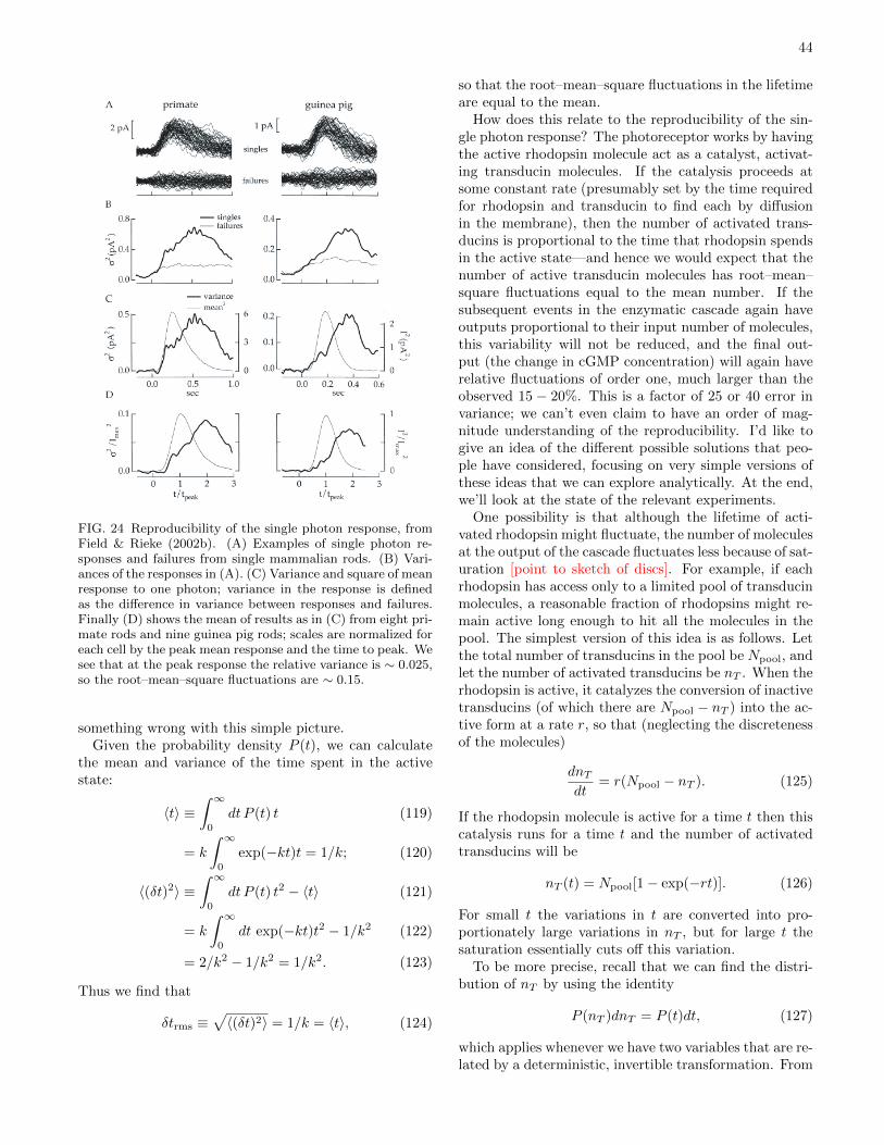
44

FIG. 24 Reproducibility of the single photon response, fromField & Rieke (2002b). (A) Examples of single photon re-sponses and failures from single mammalian rods. (B) Vari-ances of the responses in (A). (C) Variance and square of meanresponse to one photon; variance in the response is definedas the di!erence in variance between responses and failures.Finally (D) shows the mean of results as in (C) from eight pri-mate rods and nine guinea pig rods; scales are normalized foreach cell by the peak mean response and the time to peak. Wesee that at the peak response the relative variance is ! 0.025,so the root–mean–square fluctuations are ! 0.15.

something wrong with this simple picture.Given the probability density P (t), we can calculate

the mean and variance of the time spent in the activestate:

#t$ )% "

0dt P (t) t (119)

= k

% "

0exp("kt)t = 1/k; (120)

#((t)2$ )% "

0dt P (t) t2 " #t$ (121)

= k

% "

0dt exp("kt)t2 " 1/k2 (122)

= 2/k2 " 1/k2 = 1/k2. (123)

Thus we find that

(trms )"#((t)2$ = 1/k = #t$, (124)

so that the root–mean–square fluctuations in the lifetimeare equal to the mean.How does this relate to the reproducibility of the sin-

gle photon response? The photoreceptor works by havingthe active rhodopsin molecule act as a catalyst, activat-ing transducin molecules. If the catalysis proceeds atsome constant rate (presumably set by the time requiredfor rhodopsin and transducin to find each by di!usionin the membrane), then the number of activated trans-ducins is proportional to the time that rhodopsin spendsin the active state—and hence we would expect that thenumber of active transducin molecules has root–mean–square fluctuations equal to the mean number. If thesubsequent events in the enzymatic cascade again haveoutputs proportional to their input number of molecules,this variability will not be reduced, and the final out-put (the change in cGMP concentration) will again haverelative fluctuations of order one, much larger than theobserved 15 " 20%. This is a factor of 25 or 40 error invariance; we can’t even claim to have an order of mag-nitude understanding of the reproducibility. I’d like togive an idea of the di!erent possible solutions that peo-ple have considered, focusing on very simple versions ofthese ideas that we can explore analytically. At the end,we’ll look at the state of the relevant experiments.One possibility is that although the lifetime of acti-

vated rhodopsin might fluctuate, the number of moleculesat the output of the cascade fluctuates less because of sat-uration [point to sketch of discs]. For example, if eachrhodopsin has access only to a limited pool of transducinmolecules, a reasonable fraction of rhodopsins might re-main active long enough to hit all the molecules in thepool. The simplest version of this idea is as follows. Letthe total number of transducins in the pool be Npool, andlet the number of activated transducins be nT . When therhodopsin is active, it catalyzes the conversion of inactivetransducins (of which there are Npool " nT ) into the ac-tive form at a rate r, so that (neglecting the discretenessof the molecules)

dnT

dt= r(Npool " nT ). (125)

If the rhodopsin molecule is active for a time t then thiscatalysis runs for a time t and the number of activatedtransducins will be

nT (t) = Npool[1" exp("rt)]. (126)

For small t the variations in t are converted into pro-portionately large variations in nT , but for large t thesaturation essentially cuts o! this variation.To be more precise, recall that we can find the distri-

bution of nT by using the identity

P (nT )dnT = P (t)dt, (127)

which applies whenever we have two variables that are re-lated by a deterministic, invertible transformation. From

45

Eq (126) we have

t = "1

rln(1" nT /Npool), (128)

and so, going through the steps explicitly:

P (nT ) = P (t)

&&&&&dnT

dt

&&&&&

!1

(129)

= k exp("kt)1

r(Npool " nT )(130)

=k

rexp

#,k

r

-ln(1" nT /Npool)

$1

(Npool " nT )

(131)

=k

rNpool

,1" nT

Npool

-k/r!1

. (132)

[Maybe a plot to show this?] When the activation rater is small, nT always stays much less that Npool andthe power law can be approximated as an exponential.When r is large, however, the probability distributiongrows a power law singularity at Npool; for r finite thissingularity is integrable but as r - . it approaches a logdivergence, which means that essentially all of the weightwill concentrated at Npool. In particular, the relativevariance of nT vanishes as r becomes large, as promised.

This discussion has assumed that the limited numberof target molecules is set, perhaps by some fixed struc-tural domain. Depending on details, it is possible forsuch a limit to arise dynamically, as a competition be-tween di!usion and chemical reactions. In invertebratephotoreceptors, such as the flies we have met in our dis-cussion above, there is actually a positive feedback loopin the amplifier which serves to ensure that each struc-tural domain (which are more obvious in the fly receptorcells) ‘fires’ a saturated, stereotyped pulse in response toeach photon.

[Make a sketch of the di!erent models—either one bigfigure, or separate ones for each model.]

The next class of models are those that use feedback.The idea, again, is simple: If the output of the cascade isvariable because the rhodopsin molecule doesn’t “know”when to de–activate, why not link the de–activation tothe output of the cascade? Roughly speaking, count themolecules at the output and shut the rhodopsin moleculeo! when we reach some fixed count. Again let’s try thesimplest version of this. When rhodopsin is active it cat-alyzes the formation of some molecule (which might notactually be the transducin molecule itself) at rate r, andlet the number of these output molecules by x so that wesimply have

dx

dt= r, (133)

or x = rt. Let’s have the rate of deactivation of rhodopsindepend on x, so that instead of Eq (117) we have

dp(t)

dt= k[x(t)]p(t). (134)

For example, if deactivation is triggered by the cooper-ative binding of m x molecules (as in the discussion ofcGMP–gated channels), we expect that

k[x] = kmaxxm

xm0 + xm

. (135)

We can solve Eq (134) and then recover the probabilitydensity for rhodospin lifetime as before,

p(t) = exp

,"% t

0d' k[x(')]

-(136)

P (t) = k[x(t)] exp

,"% t

0d' k[x(')]

-. (137)

Again we can push through the steps:

P (t) = k[x(t)] exp

,"% t

0d' k[x(')]

-= kmax

xm(t)

xm0 + xm(t)

exp

,"kmax

% t

0d'

xm(t)

xm0 + xm(t)

-(138)

+ kmax

,t

t0

-m

exp

("kmaxt0

m+ 1

,t

t0

-m+1), (139)

where in the last step we identify t0 = x0/r and assume that t , t0.

To get a better feel for the probability distribution in Eq (139) it is useful to rewrite it as

P (t) + kmax exp ["G(t)] (140)

G(t) = "m ln

,t

t0

-+

kmaxt0m+ 1

,t

t0

-m+1

(141)

46

We can find the most likely value of the lifetime, t, byminimizing G, which of course means that the derivativemust be set to zero:

G%(t) = "m

t+ kmaxt0 ·

1

t

,t

t0

-m+1

(142)

G%(t = t) = 0 % kmaxt0 ·1

t

,t

t0

-m+1

=m

t(143)

t

t0=

,m

kmaxt0

-1/m

(144)

In particular we see that for su"ciently large kmax we willhave t , t0, consistent with the approximation above.What we really want to know is how sharp the distribu-tion is in the neighborhood of t, so we will try a seriesexpansion of G(t):

P (t) + kmax exp

#"G(t)" 1

2G%%(t)(t" t)2 " · · ·

$(145)

G%%(t) =m

t2+ (kmaxt0)m · 1

t2

,t

t0

-m+1

+ m

t2, (146)

where again in the last step we assume t << t0. Thuswe see that the distribution of lifetimes is, at least nearits peak,

P (t) + P (t) exp." m

2t2(t" t)2 " · · ·

/. (147)

This of course is a Gaussian with variance

#((t)2$ = 1

m· t2, (148)

so the relative variance is 1/m as opposed to 1 in theoriginal exponential distribution.

A concrete realization of the feedback ideacan bebuilt around the fact that the current flowing into therod includes calcium ions, and the resulting changesin calcium concentration can regulate protein kinases—proteins which in turn catalyze the attachment of phos-phate groups to other proteins—and rhodopsin shut o! isknown to be associated with phosphorylation at multiplesites. Calcium activation of kinases typically is cooper-ative, so m ! 4 in the model above is plausible. Noticethat in the saturation model the distribution of lifetimesremains broad and the response to these variations istruncated; in the feedback model the distribution of life-times itself is sharpened.A third possible model involves multiple steps in

rhodopsin de–activation. Let us imagine that rhodopsinstarts in one state and makes a transition to state 2, thenfrom state 2 to state three, and so on for K states, andthen it is the transition from state K to K + 1 that ac-tually corresponds to de–activation. Thus there are Kactive states and if the time spent in each state is ti thenthe total time spent in activated states is

t =K!

i=1

ti. (149)

Clearly the mean value of t is just the sum of the means ofeach ti, and if the transitions are independent (again, thisis what you mean when you write the chemical kineticswith the arrows and rate constants) then the variance oft will also be the sum of the variances of the individualti,

#t$ =K!

i=1

#ti$ (150)

#((t)2$ =K!

i=1

#((ti)2$. (151)

We recall from above that for each single step, #((ti)2$ =#ti$2. If the multiple steps occur at approximately equalrates, we can write

#t$ =K!

i=1

#ti$ + K#t1$ (152)

#((t)2$ =K!

i=1

#((ti)2$ =K!

i=1

#ti$2 + K#t1$2 (153)

#((t)2$#t$2 + K#t1$2

(K#t1$)2=

1

K. (154)

Thus the relative variance declines as one over the num-ber of steps, and the relative standard deviation declinesas one over the square root of the number of steps. Thisis an example of how averaging K independent eventscauses a 1/

&K reduction in the noise level.

The good news is that allowing de–activation to pro-ceed via multiple steps can reduce the variance in thelifetime of activated rhodopsin. Again our attention isdrawn to the fact that rhodopsin shut o! involves phos-phorylation of the protein at multiple sites. The badnews is that to have a relative standard deviation of! 20% would require 25 steps.It should be clear that a multistep scenario works only

if the steps are irreversible. If there are significant “back-ward” rates then progress through the multiple states be-comes more like a random walk, with an accompanyingincrease in variance. Thus each of the (many) steps in-volved in rhodopsin shut o! must involve dissipation ofa few kBT of energy to drive the whole process forward.

Problem 28: Getting the most out of multiple steps.Consider the possibility that Rhodopsin leaves its active statethrough a two step process. To fix the notation, let’s say thatthe first step occurs with a rate k1 and the second occurs with ratek2:

Rh#k1$ Rh##

k2$ inactive. (155)

Assume that we are looking at one molecule, and at time t = 0 thismolecule is in state Rh#.

(a) Write out and solve the di!erential equations for the timedependent probability of being in each of the three states.

47

(b) Use your results in [a] to calculate the probability distribu-tion for the time at which the molecule enters the inactive state.This is the distribution of “lifetimes” for the two active states.Compute the mean and variance of this lifetime as a function ofthe parameters k1 and k2.

(c) Is there a simple, intuitive argument that allows you to writedown the mean and variance of the lifetime, without solving anydi!erential equations? Can you generalize this to a scheme in whichinactivation involves N steps rather than two?

(d) Given some desired mean lifetime, is there a way of adjustingthe parameters k1 and k2 (or, more generally, k1, k2 · · · , kN ) tominimize the variance?

(e) Suppose that there is a back reaction Rh## k#1$ Rh#. Discusswhat this does to the distribution of lifetimes. In particular, whathappens if the rate k"1 is very fast? Note that “discuss” is delib-erately ambiguous; you could try to solve the relevant di!erentialequations, or to intuit the answer, or even do a small simulation[connect this problem to recent work by Escola & Paniniski].

The need for energy dissipation and the apparentlyvery large number of steps suggests a di!erent physicalpicture. If there really are something like 25 steps, thenif we plot the free energy of the rhodopsin molecule as afunction of its atomic coordinates, there is a path frominitial to final state that passes over 25 hills and valleys.Each valley must be a few kBT lower than the last, andthe hills must be many kBT high to keep the rates in theright range. This means that the energy surface is quiterough [this needs a sketch]. Now when we take one solidand slide it over another, the energy surface is rough onthe scale of atoms because in certain positions the atomson each surface “fit” into the interatomic spaces on theother surface, and then as we move by an Angstrom orso we encounter a very high barrier. If we step back andblur our vision a little bit, all of this detailed roughnessjust becomes friction between the two surfaces. Formally,if we think about Brownian motion on a rough energylandscape and we average over details on short lengthand time scales, what we will find is that the mobility orfriction coe"cient is renormalized and then the systemsbehaves on long time scales as if it were moving with thishigher friction on a smooth surface.

So if the de–activation of rhodopsin is like motion ona rough energy surface, maybe we can think about therenormalized picture of motion on a smooth surface withhigh drag or low mobility. Suppose that the active andinactive states are separated by a distance & along somedirection in the space of molecular structures, and thatmotion in this direction occurs with an e!ective mobilityµ. If there is an energy drop #E between the activeand de–activated states, then the velocity of motion isv ! µ#E/& and the mean time to make the de–activationtransition is

#t$ ! &

v! &2

µ#E. (156)

On the other hand, di!usion over this time causes aspread in positions

#((&)2$ ! 2D#t$ = 2µkBT #t$, (157)

where we make use of the Einstein relation D = µkBT .Now (roughly speaking) since the molecule is moving inconfiguration space with typical velocity v, this spread inpositions is equivalent to a variance in the time requiredto complete the transition to the de–activated state,

#((t)2$ ! #((&)2$v2

! 2µkBT

(µ#E/&)2· &2

µ#E. (158)

If we express this as a fractional variance we find

#((t)2$#t$2 ! 2µkBT

(µ#E/&)2· &2

µ#E·,µ#E

&2

-2

! 2kBT

#E. (159)

Thus when we look at the variability of the lifetime in thismodel, the e!ective mobility µ and the magntiude & of thestructural change in the molecule drop out, and the re-producibility is just determined by the amount of energythat is dissipated in the de–activation transition. Indeed,comparing with the argument about multiple steps, ourresult here is the same as expected if the number of ir-reversible steps were K ! #E/(2kBT ), consistent withthe idea that each step must dissipate more than kBT inorder to be e!ectively irreversible. To achieve a relativevariance of 1/25 or 1/40 requires dropping ! 0.6" 1 eV(recall that kBT is 1/40 eV at room temperature), whichis OK since the absorbed photon is roughly 2.5 eV.

Problem 29: Is there a theorem here? The above argu-ment hints at something more general. Imagine that we have amolecule in some state, and we ask how long it takes to arrive atsome other state. Assuming that the molecular dynamics is thatof overdamped motion plus di!usion on some energy surface, canyou show that the fractional variance in the time required for themotion is limited by the free energy di!erence between the twostates?

How do we go about testing these di!erent ideas? Ifsaturation is important, one could try either by chemicalmanipulations or by genetic engineering to prolong thelifetime of rhodospin and see if in fact the amplitudeof the single photon response is bu!ered against thesechanges. If feedback is important, one could make a listof candidate feedback molecules and to manipulate theconcentrations of these molecules. Finally, if there aremultiple steps one could try to identify the molecularevents associated with each step and perturb these eventsagain either with chemical or genetic methods. All theseare good ideas, and have been pursued by several groups.

48

FIG. 25 Variability in the single photon response with genet-ically engineered rhodopsins. (A) Wild type responses frommouse rods. Schematic shows the six phosphorylation sites,which are serine or threonine residues. In the remaining pan-els, we see responses when the number of phosphorylationsites has been reduced by mutating alanine, leaving five sites(B & C), two sites (D), one site (E), or none (F). From Doanet al (2007).

An interesting hint about the possibility of multiplesteps in the rhodopsin shuto! is the presence of multi-ple phosphorylation sites on the opsin proteins. In mice,there are six phosphorylation sites, and one can genet-ically engineer organisms in which some or all of thesesites are removed. At a qualitative level it’s quite strikingthat even knocking out one of these sites produces a no-ticeable increase in the variability of the single photon re-sponses, along with a slight prolongation of the mean re-sponse (Figs 25B & C). When all but one or two sites areremoved, the responses last a very long time, and startto look like on/o! switches with a highly variable time inthe ‘on’ state (Figs 25D & E). When there are no phos-phorylation sites, rhodopsin can still turn o!, presumablyas a result of binding another molecule (arrestin). Butnow the time to shuto! is broadly distributed, as onemight expect if there were a single step controlling thetransition.

FIG. 26 Standard deviation in the integral of the single pho-ton response, normalize by the mean. Results are shown as afunction of the number of phosphorylation sites, from experi-ments as in Fig 25; error bars are standard errors of the mean.Solid line is CV = 1/

!Np + 1, where Np is the number of

phosophorylation sites. From Doan et al (2006).

Remarkably, if we examine the responses quantita-tively, the variance of the single photon response seemsto be inversely proportional the number of these sites,exactly as in the model where deactivation involved mul-tiple steps, now identified with the multiple phosphoryla-tions (Fig 26). This really is beautiful. One of the thingsthat I think is interesting here is that, absent the discus-sion of precision and reproducibility, the multiple phos-phorylation steps might just look like complexity for itsown sake, the kind of thing that biologists point to whenthey want to tease physicists about our propensity to ig-nore details. In this case, however, the complexity seemsto be the solution to a very specific physics problem.Probably this section should end with some caveats.

Do we really think the problem of reproducibility issolved?

A general review of the cGMP cascade in rods is given by Burns& Baylor (2001). Rieke & Baylor (1996) set out to understand theorigins of the continuous noise in rods, but along the way provide abeautifully quantitative dissection of the enzymatic cascade; muchof the discussion above follows theirs. For an explanation of howsimilarity to Rhodopsin (and other G–protein coupled receptors)drove the discovery of the olfactory receptors, see Buck (2004). Forsome general background on ion channels, you can try Aidley (seenotes to Section 1.1), Johnston & Wu (1995), or Hille (2001). Astarting point for learning about how di!erent choices of channelsshape the dynamics of responses in insect photoreceptors is thereview by Weckstrom & Laughlin (1995). [There is much more tosay here, and probably even some things left to do.]

Buck 2004: Unraveling the sense of smell. LB Buck, in Les PrixNobel: Nobel Prizes 2004, T Frangsmyr, ed (Nobel Founda-tion, Stockholm, 2004).

Burns & Baylor 2001: Activation, deactivation and adaptationin vertebrate photoreceptor cells. ME Burns & DA Baylor,Annu Rev Neurosci 24, 779–805 (2001).

Hille 2001: Ion Channels of Excitable Membranes, 3rd Edition BHille (Sinuaer, Sunderland MA, 2001).

Johnston & Wu 1995: Foundations of Cellular Neurophysiol-ogy. D Johnston & SM Wu (MIT Press Cambridge, 1995).

Rieke & Baylor 1996: Molecular origin of continuous dark noisein rod photoreceptors. F Rieke & DA Baylor, Biophys J 71,2553–2572 (1996).

Weckstrom & Laughlin 1995: Visual ecology and voltagegated ion channels in insect photoreceptors. M Weckstrom& SB Laughlin, Trends Neurosci 18, 17–21 (1995).

Rieke & Baylor (1998a) provide a review of photon counting rodswith many interesting observations, including an early outline ofthe problem of reproducibility. An early e!ort to analyze the sig-nals and noise in enzymatic cascades is by Detwiler et al (2000).The idea that restricted, saturable domains can arise dynamicallyand tame the fluctuations in the output of the cascade is describedby the same authors (Ramanathan et al 2005). For invertebratephotoreceptors, it seems that reproducibility of the response tosingle photons can be traced to positive feedback mechanisms thatgenerate a stereotyped pulse of concentration changes, localized tosubstructures analogous to the disks in vertebrate rods (Pumir etal 2008).

Detwiler et al 2000: Engineering aspects of enzymatic signaltransduction: Photoreceptors in the retina. PB Detwiler,S Ramanathan, A Sengupta & BI Shraiman, Biophys J 79,2801–2817 (2000).

49

Pumir et al 2008: A Pumir, J Graves, R Ranganathan & BIShraiman, Systems analysis of the single photon responsein invertebrate photoreceptors. Proc Nat’l Acad Sci (USA)105, 10354–10359 (2008).

Ramanathan et al 2005: G–protein–coupled enzyme cascadeshave intrinsic properties that improve signal localization andfidelity. S Ramanathan, PB Detwiler, AM Sengupta & BIShraiman, Biophys J 88, 3063–3071 (2005).

Rieke & Baylor 1998a: Single–photon detection by rod cells ofthe retina. F Rieke & DA Baylor, Revs Mod Phys 70, 1027–1036 (1998).

One of the early, systematic e!orts to test di!erent models of re-producibility was by Rieke & Baylor (1998b). Many of the sameideas were revisited in mammalian rods by Field & Rieke (2002b),setting the stage for the experiments on genetic engineering of thephosphorylation sites by Doan et al (2006). More recent work fromthe same group explores the competition between the kinase andthe arrestin molecule, which binds to the phosphorylated rhodopsinto terminate its activity, showing this competition influences boththe mean and the variability of the single photon response (Doanet al 2009).

Doan et al 2007: Multiple phosphorylation sites confer repro-ducibility of the rod’s single–photon responses. T Doan,A Mendez, PB Detwiler, J Chen & F Rieke, Science 313,530–533 (2006).

Doan et al 2009: Arrestin competition influences the kineticsand variability of the single–photon responses of mammalianrod photoreceptors. T Doan, AW Azevedo, JB Hurley & FRieke, J Neurosci 29, 11867–11879 (2009).

Field & Rieke 2002: Mechanisms regulating variability of thesingle photons responses of mammalian rod photoreceptors.GD Field & F Rieke, Neuron 35, 733–747 (2002b).

Rieke & Baylor 1998a: Origing of reproducibility in the re-sponses of retinal rods to single photons. F Rieke & DABaylor, Biophys J 75, 1836–1857 (1998).

D. The first synapse, and beyond

This is a good moment to remember a key feature ofthe Hecht, Shlaer and Pirenne experiment, as describedin Section I.A. In that experiment, observers saw flashesof light that delivered just a handful of photons spreadover an area that includes many hundreds of photore-ceptor cells. One consequence is that a single receptorcell has a very low probability of counting more than onephoton, and this is how we know that these cells mustrespond to single photons. But, it must also be possiblefor the retina to add up the responses of these many cellsso that the observer can reach a decision. Importantly,there is no way to know in advance which cells will get hitby photons, so if we (sliding ourselves into the positionsof the observer’s brain ... ) want to integrate the multiplephoton counts we have to integrate over all the receptorsin the area covered by the flash. This integration mightbe the simplest computation we can imagine for a ner-vous system, just adding up a set of elementary signals,all given the same weight. In many retinas, a large part

rod

photoreceptors

bipolar cells

ganglion cells

axon in the

optic nerve

horizontal

cells

FIG. 27 A schematic of the circuitry in the retina. Fill incaption.

of the integration is achieved in the very first step of pro-cessing, as many rod cells converge and form synapsesonto onto a single bipolar cell, as shown schematically inFig 27 [maybe also need a real retina?]If each cell generates an output ni that counts the num-

ber of photons that have arrived, then it’s trivial thatthe total photon count is ntotal =

0i ni. The problem

is that the cells don’t generate integers corresponding tothe number of photons counted, they generate currentswhich have continuous variations. In particular, we haveseen that the mean current in response to a single pho-ton has a peak of I1 ! 1 pA, but this rests on continuousbackground noise with an amplitude (Irms ! 0.1 pA. Ina single cell, this means that the response to one pho-ton stands well above the background, but if we try tosum the signals from many cells, we have a problem, asillustrated in Fig 28.To make the problem precise, let’s use xi to denote the

peak current generated by cell i. We have

xi = I1ni + .i, (160)

where ni is the number of photons that are counted incell i, and .i is the background current noise; from whatwe have seen in the data, each .i is chosen independentlyfrom a Gaussian distribution with a standard deviation(Irms. If we sum the signals generated by all the cells,we obtain

xtotal )Ncells!

i=1

xi = I1

Ncells!

i=1

ni +Ncells!

i=1

.i (161)

= I1ntotal + .e! , (162)

where the e!ective noise is the sum of Ncells independentsamples of the .i, and hence has a standard deviation

.rmse! )

1#.2e!$ =

"Ncells(Irms. (163)

50

! "!! #!! $!! %!! &!!

!!'#

!

!'#

!'%

!'(

!')

"

*+,,-./0+1

2+34-*566+/7-829:

! "!! #!! $!! %!! &!!

!!'#

!

!'#

!'%

!'(

!')

"

*+,,-./0+1

FIG. 28 Simulation of the peak currents generated by N =500 rod cells in response to a dim flash of light. At left,five of the cells actually detect a photon, each resulting in acurrent I1 ! 1 pA, while at right we see the response to ablank. All cells have an additive background noise, chosenfrom a Gaussian distribution with zero mean and standarddeviation "Irms ! 0.1 pA. Although the single photon re-sponses stand clearly above the background noise, if we sim-ply add up the signals generated by all the cells, then at leftwe find a total current Itotal = 1.85 pA, while at right we findItotal = 3.23 pA—the summed background noise completelyoverwhelms the signal.

The problem is that with (Irms ! 0.1 pA and Ncells =500, we have .rms

e! ! 2.24 pA, which means that thereis a sizable chance of confusing three or even five pho-tons with a blank; in some species, the number of cellsover which the system integrates is even larger, and theproblem becomes even more serious. Indeed, in primateslike us, a single ganglion cell (one stage after the bipolarcells; cf Fig 27) receives input from ! 4000 rods, whileon a very dark night we can see when just one in a thou-sand rods is captures a photon [should have refs for allthis]. Simply put, summing the signals from many cellsburies the clear single photon response under the noisegenerated by those cells which did not see anything. Thiscan’t be the right way to do things!

Before we start trying to do something formal, let’sestablish some intuition. Since the single photon signalsare clearly detectable in individual rod cells, we couldsolve our problem by making a ‘decision’ for each cell—is there a photon present or not?—and then adding upthe tokens that represent the outcome of our decision.Roughly speaking, this means passing each rod’s sig-nal through some fairly strong nonlinearity, perhaps sostrong that it has as an output only a 1 or a 0, and thenpooling these nonlinearly transformed signals. In con-trast, a fairly standard schematic of what neurons aredoing throughout the brain is adding up their inputs andthen passing this sum through a nonlinearity (Fig 29).

So perhaps the problems of noise in photon counting areleading us to predict that this very first step of neuralcomputation in the retina has to be di!erent from thisstandard schematic. Let’s try to do an honest calculationthat makes this precise. [Is “nonlinearity” clear enoughhere?]Formally, the problem faced by the system is as follows.

We start with the set of currents generated by all the rodcells, {xi}. We can’t really be interested in the currentsthemselves. Ideally we want to know about what is hap-pening in the outside world, but a first step would be toestimate the total number of photons that arrived, ntotal.What is the best estimate we can make? To answer this,we need to say what we mean by “best.”One simple idea, which is widely used, is that we want

to make estimates which are as close as possible to theright answer, where closeness is measured by the meansquare error. That is, we want to map the data {xi} intoan estimate of ntotal through some function nest ({xi})such that

E )2[ntotal " nest ({xi})]2

3(164)

is as small as possible. To find the optimal choice of thefunction nest ({xi}) seems like a hard problem—maybewe have to choose some parameterization of this function,and then vary the parameters? In fact, we can solve thisproblem once and for all, which is part of the reason thatthis definition of ‘best’ is popular.

When we compute our average error, we are averagingover the joint distribution of the data {xi} and the actual

!

!

rod photoreceptors

bipolar cell voltage? bipolar cell voltage?

FIG. 29 Schematic of summation and nonlinearity in the ini-tial processing of rod cell signals. At left, a conventionalmodel in which many rods feed into one bipolar cell; the bipo-lar cell sums its inputs and passes the results through a satu-rating nonlinearity. At right, an alternative model, suggestedby the problems of noise, in which nonlinearities precede sum-mation.

51

photon count ntotal. That is,

E )2[n" nest ({xi})]2

3

=

% (Ncells4

i=1

dxi

)!

ntotal

P (n, {xi}) [n" nest ({xi})]2 ,(165)

where, to simplify the notation, we drop the subscripttotal. Now to minimize the error we take the variationwith respect to the function nest ({xi}) and set the resultequal to zero. We have

(E(nest ({xi})

= "!

n

P (n, {xi})2 [n" nest ({xi})] ,

(166)so setting this to zero gives (going through the steps care-fully):

!

n

P (n, {xi})nest ({xi}) =!

n

P (n, {xi})n (167)

nest ({xi})!

n

P (n, {xi}) =!

n

P (n, {xi})n (168)

nest ({xi})P ({xi})!

n

P (n, {xi})n (169)

nest ({xi}) =!

n

P (n, {xi})P ({xi})

n, (170)

and, finally,

nest ({xi}) =!

n

P (n|{xi})n. (171)

Thus the optimal estimator is the mean value in the con-ditional distribution, P (n|{xi}). Since we didn’t use anyspecial properties of the distributions, this must be truein general, as long as ‘best’ means to minimize meansquare error. We’ll use this result many times, and comeback to the question of whether the choice of mean squareerror is a significant restriction.

Notice that the relevant conditional distribution is thedistribution of photon counts given the rod cell currents.From a mechanistic point of view, we understand theopposite problem, that is, given the photon counts, weknow how the currents are being generated. More pre-cisely, we know that, given the number of photons ineach cell, the currents will be drawn out of a probabilitydistribution, since this is (implicitly) what we are sayingwhen we write Eq (160). To make this explicit, we have

P ({xi}|{ni}) * exp

("1

2

Ncells!

i=1

,xi " I1ni

(Irms

-2). (172)

Again, this is a model that tells us how the photons gen-erate currents. But the problem of the organism is touse the currents to draw inferences about the photons.

We expect that since the signals are noisy, this infer-ence will be probabilistic, so really we would like to knowP ({ni}|{xi}).

Problem 30: Just checking. Be sure that you understandthe connection between Eq (172) and Eq (160). In particular, whatassumptions are crucial in making the connection?

The problem of going from P ({xi}|{ni}) toP ({ni}|{xi}) is typical of the problems faced byorganisms: given knowledge of how our sensory datais generated, how do we reach conclusions about whatreally is going on in the outside world? In a sensethis is the same problem that we face in doing physicsexperiments. One could argue that what we have posedhere is a very easy version of the real problem. In fact,we probably don’t really care about the photon arrivals,but about the underlying light intensity, or more deeplyabout the identity and movements of the objects fromwhich the light is being reflected. Still, this is a goodstart.The key to solving these inference problems, both for

organisms and for experimental physicists, is Bayes’ rule.Imagine that we have two events A and B; to be concrete,we could think of A as some data we observe, and B as avariable in the world that we really want to know. Thereis some probability P (A,B) that both of these are truesimultaneously, i.e. that we observe A and the world isin state B. In the usual view, the states of the worldcause the data to be generated in our instruments, so wecan say that the state of the world is chosen out of somedistribution P (B), and then given this state the data aregenerated, with some noise, and hence drawn out of theconditional distribution P (A|B). By the usual rules ofprobability, we have

P (A,B) = P (A|B)P (B). (173)

We could also imagine that we have just seen the dataA, drawn out of some distribution P (A), and then theremust be some distribution of things happening in theworld that are consistent with our observation. Formally,

P (A,B) = P (B|A)P (A). (174)

But these are just two di!erent ways of decomposing thejoint distribution P (A,B), and so they must be equal:

P (A,B) = P (B|A)P (A) = P (A|B)P (B) (175)

P (B|A) =P (A|B)P (B)

P (A). (176)

52

This last equation is called Bayes’ rule, and tells us whatwe need to know. It is useful to rewrite this, takingseriously the case where A refers to measurable data andB refers to the state of the world:

P (world|data) = P (data|world)P (world)

P (data). (177)

Equation (177) is telling us that the probability of theworld being in a certain state is proportional to the prob-ability that this state could generate the data we haveseen, but this is multiplied by the overall probability thatthe world can be in this state. This term often is re-ferred to as the ‘prior’ probability, since it summarizesour knowledge prior to the observation of the data. Putanother way, our inference about the world should beboth consistent with the data we have observed in thisone experiment and with any prior knowledge we mighthave from previous data.23

Applied to our current problem, Bayes’ rule tells ushow to construct the probability distribution of photoncounts given the rod currents:

P ({ni}|{xi}) =P ({xi}|{ni})P ({ni})

P ({xi}). (178)

To make progress (and see how to use these ideas), let’sstart with the simple case of just one rod cell, so we candrop the indices:

P (n|x) = P (x|n)P (n)

P (x). (179)

To keep things really simple, let’s just think about thecase where the lights are very dim, so either there arezero photons or there is one photon, so that

P (1|x) = P (x|1)P (1)

P (x), (180)

and similarly for P (0|x). In the denominator we haveP (x), which is the probability that we will see the currentx, without any conditions on what is going on in theworld. We get this by summing over all the possibilities,

P (x) =!

n

P (x|n)P (n) (181)

= P (x|1)P (1) + P (x|0)P (0), (182)

where in the last step we use the approximation that thelights are very dim. Putting the terms together, we have

P (1|x) = P (x|1)P (1)

P (x|1)P (1) + P (x|0)P (0). (183)

Now we can substitute for P (x|n) from Eq (172),

P (x|n) = 1"2$((Irms)2

exp

#" (x" I1n)2

2((Irms)2

$. (184)

Going through the steps, we have

P (1|x) = P (x|1)P (1)

P (x|1)P (1) + P (x|0)P (0)=

1

1 + P (x|0)P (0)/P (x|1)P (1)(185)

=1

1 + [P (0)/P (1)] exp." (x)2

2(&Irms)2+ (x!I1)2

2(&Irms)2

/ =1

1 + exp (% " /x), (186)

where

% = ln

#P (0)

P (1)

$+

I212((Irms)2

(187)

/ =I1

((Irms)2. (188)

The result in Eq (186) has a familiar form—it is as ifthe two possibilities (0 and 1 photon) are two states ofa physical system, and their probabilities are determinedby a Boltzmann distribution; the energy di!erence be-tween the two states shifts in proportion to the data x,and the temperature is related to the noise level in thesystem. In the present example, this analogy doesn’t addmuch, essentially because the original problem is so sim-ple, but we’ll see richer cases later on in the course.

Equation (186) tells us that, if we observe a very smallcurrent x, the probability that there really was a photonpresent is small, ! e!". As the observed current becomeslarger, the probability that a photon was present goes up,and, gradually, as x becomes large, we become certain[P (1|x) - 1]. To build the best estimator of n fromthis one cell, our general result tells us that we shouldcompute the conditional mean:

nest(x) =!

n

P (n|x)n (189)

= P (0|x) · (0) + P (1|x) · (1) (190)

= P (1|x). (191)

Thus, the Boltzmann–like result [Eq (186)] for the prob-ability of a photon being counted is, in fact, our best

53

estimator of the photon count in this limit where pho-tons are very rare. Further, in this limit one can showthat the optimal estimator for the total photon count,which after all is the sum of the individual ni, is just thesum of the individual estimators.

Problem 31: Summing after the nonlinearity. Show thatthe optimal estimator for the total number of photons is the sum ofestimators for the photon counts in individual rods, provided thatthe lights are very dim and hence photons are rare. The phrasinghere is deliberately vague—you should explore the formulation ofthe problem, and see exactly what approximations are needed tomake things come out right.

The end result of our calculations is that the optimalestimator of photon counts really is in the form shownat the right in Fig 29: nonlinearities serve to separatesignal from noise in each rod cell, and these ‘cleaned’ sig-nals are summed. How does this prediction compare withexperiment? Careful measurements in the mouse retinashow that the bipolar cells respond nonlinearly even tovery dim flashes of light, in the range where the rods seesingle photons and respond linearly, with two photonsproducing twice the response to one photon. The formof the nonlinearity is what we expect from the theory,a roughly sigmoidal function that suppresses noise andpasses signals only above an amplitude threshold. Im-portantly, this nonlinearity is observed in one class ofbipolar cells but not others, and this is the class that,on other grounds, one would expect is most relevant forprocessing of rod outputs at low light levels.

Looking more quantitatively at the experiments [showsome of the data, perhaps replotted in di!erent forms ...go back and look at the original papers and clean up thisparagraph!], we can see discrete, single photon events inthe bipolar cells. Although the details vary across organ-isms, in this retina, one bipolar cell collects input from! 20 rod cells, but the variance of the background noiseis larger than in the lower vertebrates that we first sawin Fig 4. As a result, if we sum the rod inputs and passthem through the observed nonlinearity—as in the modelat left in Fig 29—we would not be able to resolve the sin-gle photon events. Field and Rieke considered a family ofmodels in which the nonlinearity has the observed shapebut the midpoint (analogous to the threshold % above)is allowed to vary, and computed the signal to noise ra-tio at the bipolar cell output for the detection of flashescorresponding to a mean count of ! 10!4 photons/rodcell, which is, approximately, the point at which we canbarely see something on a moonless night. Changing thethreshold by a factor of two changes the signal to noiseratio by factors of several hundred. The measured value

of the threshold is within 8% of the predicted optimalsetting, certainly close enough to make us think that weare on the right track.The discussion thus far has emphasized separating sig-

nals from noise by their amplitudes.24 We also can see,by looking closely at the traces of current vs time, thatsignal and noise have di!erent frequency content. Thissuggests that we could also improve the signal to noise ra-tio by filtering. It’s useful to think about a more generalproblem, in which we observe a time dependent signaly(t) that is driven by some underlying variable x(t); let’sassume that the response of y to x is linear, but noisy, sothat

y(t) =

% "

!"d' g(')x(t" ') + .(t), (192)

where g(') describes the response function and .(t) is thenoise. What we would like to do is to use our observationson y(t) to estimate x(t).

Problem 32: Harmonic oscillator revisited. Just to be sureyou understand what is going in Eq (192), think again about theBrownian motion of a damped harmonic oscillator, as in Problem[**], but now with an external force F (t),

md2x(t)

dt2+ +

dx(t)

dt+ *x(t) = F (t) + (F (t). (193)

Show that

x(t) =

0 !

"!d! g(!)F (t! !) + ,(t). (194)

Derive an explicit expression for the Fourier transform of g(!), andfind g(!) itself in the limit of either small or large damping +.

Since the y is linearly related to x, we might guessthat we can make estimates using some sort of linear op-eration. As we have seen already in the case of the rodcurrents, this might not be right, but let’s try anyway—we’ll need somewhat more powerful mathematical toolsto sort out, in general, when linear vs nonlinear compu-tations are the most useful. We don’t have any reason toprefer one moment of time over another, so we should dosomething that is both linear and invariant under timetranslations, which means that our estimate must be ofthe form

xest(t) =

% "

!"dt% f(t" t%)y(t%), (195)

24 Need to be a little careful here, since the analysis from Fred’ labactually involves applying the nonlinearity to voltages that havealready been filtered. Presumably this will be clearer when I ampointing to the real data .. come back and fix this!

54

where f(t) is the ‘filter’ that we hope will separate signaland noise. Following the spirit of the discussion above,we’ll ask that our estimate be as close as possible to theright answer in the sense of mean–square error. Thus,our task is to find the filter f(t) that minimizes

E =

2#x(t)"

% "

!"dt% f(t" t%)y(t%)

$2 3. (196)

In taking the expectation value of the mean–squareerror, we average over possible realizations of the noiseand the variations in the input signal x(t). In practicethis averaging can also be thought of as including anaverage over time.25 Thus we can also write

E =

2% "

!"dt

#x(t)"

% "

!"dt% f(t" t%)y(t%)

$2 3. (197)

This is useful because we can then pass to the Fourierdomain. We recall that for any function z(t),

% "

!"dt z2(t) =

% "

!"

d!

2$

&&z(!)&&2, (198)

and that the Fourier transform of a convolution is theproduct of transforms,

% "

!"dt e+i#t

% "

!"dt% f(t" t%)y(t%) = f(!)y(!). (199)

Putting things together, we can rewrite the mean–squareerror as

E =

2% "

!"

d!

2$

&&&&x(!)" f(!)y(!)

&&&&23

. (200)

Now each frequency component of our filter f(!) ap-pears independently of all the others, so minimizing Eis straightforward. The result is that

f(!) =#y#(!)x(!)$#|y(!)|2$ . (201)

Problem 33: Details of the optimal filter. Fill in the stepsleading to Eq (201). Be careful about the fact that f(t) is real, andso the transform f(") is not arbitrary. Hint: think about positiveand negative frequency components.

25 More formally, if all the relevant random variations are ergodic,then averaging over the distributions and averaging over timewill be the same.

To finish our calculation, we go back to Eq (192), whichin the frequency domain can be written as

y(!) = g(!)x(!) + .(!). (202)

Thus

#y#(!)x(!)$ = g#(!)#|x(!)|2$ (203)

#|y(!)|2$ = |g(!)|2#|x(!)|2$+ #|.(!)|2$. (204)

If all of these variables have zero mean (which we canhave be true just by choosing the origin correctly), thenquantities such as #|x(!)|2$ are the variances of Fouriercomponents, which we know (see Appendix B) are pro-portional to power spectra. Finally, then, we can substi-tute into our expression for the optimal filter to find

f(!) =g#(!)Sx(!)

|g(!)|2Sx(!) + S'(!), (205)

where, as before, Sx and S' are the power spectra of xand ., respectively.In the case that noise is small, we can let S' - 0 and

we find

f(!) - 1

g(!). (206)

This means that, when noise can be neglected, the bestway to estimate the underlying signal is just to invertthe response function of our sensor, which makes sense.Notice that since g generally serves to smooth the timedependence of y(t) relative to that of x(t), the filterf(!) ! 1/g(!) undoes this smoothing. This is impor-tant because it reminds us that smoothing in and of it-self does not set a limit to time resolution—it is only thecombination of smoothing with noise that obscures rapidvariations in the signal.Guided by the limit of high signal to noise ratio, we

can rewrite the optimal filter as

f(!) =1

g(!)· |g(!)|2Sx(!)

|g(!)|2Sx(!) + S'(!)(207)

=1

g(!)· SNR(!)

1 + SNR(!), (208)

where we identify the signal to noise ratio at each fre-quency, SNR(!) = |g(!)|2Sx(!)/S'(!). Clearly, as thesignal to noise ratio declines, so does the optimal filter—in the limit, if SNR(!) = 0, everything we find at fre-quency ! must be noise, and so it should zeroed out if wewant to minimize its corrupting e!ects on our estimates.In the case of the retina, x is the light intensity, and

y are the currents generated by the rod cells. When it’svery dark outside, the signal to noise ratio is low, so that

f(!) - g#(!)

S'(!)· Sx(!). (209)

55

The filter in this case has two pieces, one of which de-pends only on the properties of the rod cell,

f1(!) =g#(!)

S'(!), (210)

and another piece that depends on the power spectrumof the time dependent light intensity, Sx(!). With a bitmore formalism we can show that this first filter, f1(!),has a universal meaning, so that if instead of estimatingthe light intensity itself, we try to estimate somethingelse—e.g., the velocity of motion of an object across thevisual field—then the first step in the estimation processis still to apply this filter. So, it is a natural hypothesisthat this filter will be implemented near the first stagesof visual processing, in the transfer of signals from therods to the bipolar cells.

FIG. 30 Voltage responses of rod and bipolar cells in the sala-mander retina, compared with theory, from Rieke et al (1991).The theory is that the transmission from rod currents to bipo-lar cell voltage implements the optimal filter as in Eq (210).Measured responses are averages over many presentations ofa flash at t = 0 that results in an average of five photons be-ing counted. The predicted filter is computed from measuredsignal and noise properties of the rod cell, with no adjustableparameters.

Problem 34: Filtering the real rod currents. Theraw data that were used to generate Fig 4 are available athttp://www.princeton.edu/#wbialek/PHY562/data.html, in thefile rodcurrents.mat. The data consist of 395 samples of the rodcurrent in response to dim flashes of light. The data are sampledin 10ms bins, and the flash is delivered in the 100th bin. If theseideas about filtering are sensible, we should be able to do a betterjob of discriminating between zero, one and two photons by usingthe right filter. Notice that filtering of a response that is lockedto a particular moment in time is equivalent to taking a weightedlinear combination of the currents at di!erent times relative to theflash. Thus you can think of the current in response to one flashas a vector, and filtering amounts to taking the dot product of thisvector with some template. As a first step, you should reproducethe results of Fig 4, which are based just on averaging points inthe neighborhood of the peak. Under some conditions, the best

template would just be the average single photon response. Howwell does this work? What conditions would make this work best?Can you do better? These data are from experiments by FM Riekeand collaborators at the University of Washington, and thanks toFred for making them available.

The idea that the rod/bipolar synapse implements anoptimal filter is interesting not least because this leads usto a prediction for the dynamics of this synapse, Eq (210),which is written entirely in terms of the signal and noisecharacteristics of the rod cell itself. All of these proper-ties are measurable, so there are no free parameters inthis prediction.26 To get some feeling for how these pre-dictions work, remember that the noise in the rod cellhas two components—the spontaneous isomerizations ofrhodopsin, which have the same frequency content as thereal signal, and the continuous background noise, whichextends to higher frequency. If we have only the sponta-neous isomerizations, then S' ! |g|2, and we are againin the situation where the best estimate is obtained by‘unsmoothing’ the response, essentially recovering sharppulses at the precise moments when photons are ab-sorbed. This unsmoothing, or high–pass filtering, is cuto! by the presence of the continuous background noise,and the di!erent e!ects combine to make f1 a band–passfilter. By the time the theory was worked out, it wasalready known that something like band–pass filteringwas happening at this synapse; among other things thisspeeds up the otherwise rather slow response of the rod.In Fig 30 we see a more detailed comparison of theoryand experiment.

Problem 35: Optimal filters, more rigorously. Severalthings were left out of the optimal filter analysis above; let’s try toput them back here.

(a.) Assume that there is a signal s(t), and we observe, in thesimplest case, a noisy version of this signal, y(t) = s(t) + ,(t).Let the power spectrum of s(t) be given by S("), and the powerspectrum of the noise ,(t) be given by N("). Further, assumethat both signal and noise have Gaussian statistics. Show that thedistribution of signals given our observations is

P [s(t)|y(t)] =1

Zexp

.!1

2

0d"

2&

|s(")! y(")|2

N(")!

1

2

0d"

2&

|s(")|2

S(")

/.

(211)

26 We should be a bit careful here. The filter, as written, is notcausal. Thus, to make a real prediction, we need to shift the filterso that it doesn’t have any support at negative times. To make awell defined prediction, we adopt the minimal delay that makesthis work. One could perhaps do better, studying the optimalfiltering problem with explicitly causal filters, and consideringthe tradeo! between errors and acceptable delays.

56

(b.) Show that the most likely function s(") given the data ony is also the best estimate in the least squares sense, and is givenby

s(nc)est (") =

S(")

S(") +N(")y("); (212)

the superscript (nc) reminds us that this estimate does not respectcausality. Show that this is consistent with Eq (205). Notice thatyou didn’t assume the optimal estimator was linear, so you haveshown that it is (!). Which of the assumptions here are essential inobtaining this result?

(c.) The non–causal estimator is Eq (212) is constructed byassuming that we have access to the entire function y(t), with!. < t < ., as we try to estimate, for example s(t = 0). Ifwe want our estimator to be something that we can build, then wemust impose causality: the estimate of s(t) can be based only onthe history y" ( y(t$ < t). Another way of saying this is that wedon’t really know y+ ( y(t$ > t), so we should average over thispart of the trajectory. But the average should be computed in thedistribution P [y+|y"]. To construct this, start by showing that

P [y+, y"] ( P [y(t)] =1

Z0exp

.!1

2

0d"

2&

|y(")|2

S(") +N(")

/. (213)

(d.) Recall that when we discuss causality, it is useful to thinkabout the frequency " as a complex variable. Explain why we canwrite

1

S(") +N(")= |$(")|2, (214)

where $(") has no poles in the upper half of the complex " plane.Verify that, with this decomposition,

$(t) =

0d"

2&e"i$t$(") (215)

is causal, that is $(t < 0) = 0. Consider the case where the signalhas a correlation time !c, so that S(") = 2'2!c/[1 + ("!c)2], andthe noise is white N(") = N0; construct $(") explicitly in thiscase.

(e.) Putting Eq (213) together with Eq (214), we can write

P [y+, y"] =1

Z0exp

1!1

2

0d"

2&

""""y(")$(")""""22. (216)

Show that

P [y+, y"] =1

Z0exp

3

4!1

2

0 0

"!dt

"""""

0d"

2&e"i$ty"(")$(")

"""""

2

!1

2

0 !

0dt

"""""

0d"

2&e"i$t(y"(") + y+("))$(")

"""""

25

6 , (217)

and that

P [y+|y"] + exp

3

4!1

2

0 !

0dt

"""""

0d"

2&e"i$t(y"(") + y+("))$(")

"""""

25

6 .

(218)Explain why averaging over the distribution P [y+|y"] is equivalentto imposing the “equation of motion”

0d"

2&e"i$t(y"(") + y+("))$(") = 0 (219)

at times t > 0.(f.) Write the non–causal estimate Eq (212) in the time domain

as

s(nc)est (t) =

0d"

2&e"i$t$#(")$(")y("). (220)

But the combination $(")y(") is the Fourier transform of z(t),which is the convolution of $(t) with y(t). Show that Eq (219)implies that the average of z(t) is the distribution P [y+|y"] van-ishes for t > 0, and hence the averaging over y+ is equivalent toreplacing

$(")y(") $0 0

"!d!ei$!

0d"$

2&$("$)y("$)e"i$"! (221)

in Eq (212). Put all the pieces together to show that there is acausal estimate of s(t) which can be written as

sest(t) =

0d"

2&e"i$tk(")y("), (222)

where

k(") = $(")

0 !

0d!ei$!

0d"$

2&e"i$"!S("$)$#("$). (223)

Verify that this filter is causal.

It is worth noting that we have given two very di!erentanalyses. In one, signals and noise are separated by linear

filtering. In the other, the same separation is achievedby a static nonlinearity, applied in practice to a linearlyfiltered signal. Presumably there is some more generalnonlinear dynamic transformation that really does thebest job. We expect that the proper mix depends on thedetailed spectral structure of the signals and noise, andon the relative amplitudes of the signal and noise, whichmight be why the di!erent e!ects are clearest in retinasfrom very di!erent species. Indeed, there is yet anotherapproach which emphasizes that the dynamic range ofneural outputs is limited, and that this constrains howmuch information the second order neuron can provideabout visual inputs; filters and nonlinearities can be cho-sen to optimize this information transmission across awide range of background light intensities, rather thanfocusing only on the detectability of the dimmest lights.This approach has received the most attention in inverte-brate retinas, such as the fly that we met near the end ofSection I.A, and we will return to these ideas in Chapter4. It would be nice to see this all put together correctly,and this is an open problem, surely with room for somesurprises.So far we have followed the single photon signal from

the single rhodopsin molecule to the biochemical networkthat amplifies this molecular event into a macroscopiccurrent, and then traced the processing of this electricalsignal as it crosses the first synapse. To claim that wehave said anything about vision, we have to at least fol-low the signal out of the retina and on its way to thebrain. [By now we should have said more about retinalanatomy—optic nerve, made up of the axons from ‘reti-nal ganglion cells,’ and the stereotyped action potentials

57

that propagate along these axons. Should also discusstechniques for picking up the signals, up to current workwith electrode arrays. Show a modern figure, e.g. fromBerry’s lab.]

The classic experiments on single photon responses inretinal ganglion cells were done well before it was possibleto measure the responses of single rods. The spikes fromsingle ganglion cells are relatively easy to record, andone can try to do something like the Hecht, Shlaer andPirenne experiment, but instead of “seeing” (as in Fig2), you just ask if you can detect the spikes. There werea number of hints in the data that a single absorbedphoton generated more than one spike, so some care isrequired. As shown in Fig 31, there are neurons thatseem to count by threes—if you wait for three spikes,the probability of seeing is what you expect for settinga threshold of K = 1 photon, if you wait for six spikesit is as if K = 2, and so on. This simple linear relationbetween photons and spikes also makes it easy to estimatethe rate of spontaneous photon–like events in the dark.Note that if photons arrive as a Poisson process, andeach photon generates multiple spikes, then the spikesare not a Poisson process; this idea of Poisson eventsdriving a second point process to generate non–Poissonvariability has received renewed attention in the contextof gene expression, where the a single messenger RNAmolecule (perhaps generated from a Poisson process) canbe translated to yield multiple protein molecules.

FIG. 31 A frequency of seeing experiment with spikes, fromBarlow et al (1971). Recording from a single retinal ganglioncell, you can say you “saw” a flash when you detect 3, 6, 9, ...or more spikes within a small window of time (here, 200 ms).The probability of reaching this criterion is plotted vs thelog of the flash intensity, as in the original Hecht, Shlaer andPirenne experiments (Fig 2), but here the intensity is adjustedto include a background rate of photon–like events (“darklight”). Curves are from Eq (2), with the indicated values ofthe threshold K. Notice that three spikes corresponds to onephoton.

Problem 36: Poisson–driven bursts. A characteristic fea-ture of events drawn out of a Poisson process is that if we countthe number of events, the variance of this number is equal to themean. Suppose that each photon triggers exactly b spikes. Whatis the ratio of variance to mean (sometimes called the Fano factor)for spike counts in response to light flashes of fixed intensity? Sup-pose the the burst of spikes itself is a Poisson process, with meanb. Now what happens to the variance/mean ratio?

Before tracing the connections between individualspikes and photons, it was possible to do a di!erent ex-periment, just counting spikes in response to flashes ofdi!erent intensities, and asking what is the smallest valueof the di!erence #I such that intensities I and I + #Ican be distinguished reliably. The answer, of course, de-pends on the background intensity I [show figure fromBarlow (1965)?]. For su"ciently small I, the just no-ticeable di!erent #I is constant. For large I, one finds#I * I, so the just noticeable fractional change in in-tensity is constant; this is common to many perceptualmodalities, and is called Weber’s law. At intermediate in-tensities one can see#I *

&I. This last result, predicted

by Rose and de Vries (cf Section 1.1), is what you expectif detecting a change in intensity just requires discrimi-nating against the Poisson fluctuations in the arrival ofphotons. At high intensities, we are counting many pho-tons, and probably the system just can’t keep up; thenfluctuations in the gain of the response dominate, andthis can result in Weber’s law. At the lowest intensities,the photons delivered by the flash are few in compari-son with the thermal isomerizations of Rhodopsin, andthis constant noise source sets the threshold for discrim-ination. Happily, the rate of spontaneous isomerizationsestimated from these sorts of experiments agrees withother estimates, including the (much later) direct mea-surements on rod cells discussed previously. This workon discrimination with neurons also is important becauseit represents one of the first e!orts to connect the per-ceptual abilities of whole organisms with the response ofindividual neurons.If retinal ganglion cells generate three spikes for every

photon, lights wouldn’t need to be very bright before thecells should be generating thousands of spikes per second,and this is impossible—the spikes themselves are roughlyone millisecond in duration, and all neurons have a ‘re-fractory period’ that defines a minimum time (like a hardcore repulsion) between successive action potentials. Theanswer is something we have seen already in the voltageresponses of fly photoreceptors (Fig 13): as the back-ground light intensity increases, the retina adapts andturns down the gain, in this case generating fewer spikesper photon. Of course this takes some time, so if we

58

suddenly expose the retina to a bright light there is veryrapid spiking, which then adapts away to a much slowerrate. [Need a figure about light/dark adaptation.] If weimagine that our perceptions are driven fairly directly bythe spikes, then our impression of the brightness of thelight should similarly fade away. This is true not just forlight (as you experience whenever you walk outside on abright sunny day); almost all constant sensory inputs getadapted away—think about the fact that you don’t feelthe pressure generated by your shoes a few minutes afteryou tie them. But there are more subtle issues as well,involving the possibility that the coding strategy usedby the retina adapts to the whole distribution of inputsrather than just the mean; this is observed, and manysubsequent experiments are aimed at understanding themolecular and cellular mechanisms of these e!ects. Thepossibility that adaptation serves to optimize the e"-ciency of coding continuous signals into discrete spikes issomething we will return to in Chapter 4.

The problem of photon counting—or any simple de-tection task—also hides a deeper question: how does thebrain “know” what it needs to do in any given task? Evenin our simple example of setting a threshold to maximizethe probability of a correct answer, the optimal observermust at least implicitly acquire knowledge of the rele-vant probability distributions. Along these lines, thereis more to the ‘toad cooling’ experiment than a test ofphoton counting and dark noise. The retina has adap-tive mechanisms that allow the response to speed up athigher levels of background light, in e!ect integrating forshorter times when we can be sure that the signal tonoise ratio will be high. The flip side of this mechanismis that the retinal response slows down dramatically inthe dark [connect back to photoreceptor responses; a fig-ure here would be good, including ' vs I relevant to Ahoet al]. In moderate darkness (dusk or bright moonlight)the slowing of the retinal response is reflected directly ina slowing of the animal’s behavior. It is as if the toadexperiences an illusion because images of its target aredelayed, and it strikes at the delayed image. It is worthemphasizing that we see a closely related illusion.

Problem 37: Knowing where to look. Give a problem toillustrate the role of uncertainty in reducing performance.

Imagine watching a pendulum swinging while wearingglasses that have a neutral density filter over one eye,so the mean light intensity in the two eyes is di!erent.The dimmer light results in a slower retina, so the signalsfrom the two eyes are not synchronous, and recall thatdi!erences in the images between our right and left eyes

are cues to the depth of an object. As we try to inter-pret these signals in terms of motion, we find that evenif the pendulum is swinging in a plane parallel to theline between our eyes, what we see is motion in 3D. Themagnitude of the apparent depth of oscillation is relatedto the neutral density and hence to the slowing of signalsin the ‘darker’ retina. This is called the Pulfrich e!ect.If the pattern of delay vs light intensity continued down

to the light levels in the darkest night, it would be adisaster, since the delay would mean that the toad in-evitably strikes behind the target! In fact, the toad doesnot strike at all in the first few trials of the experimentin dim light, and then strikes well within the target. Itis hard to escape the conclusion that the animal is learn-ing about the typical velocity of the target and then us-ing this knowledge to extrapolate and thereby correct forretinal delays.27 Thus, performance in the limit wherewe count photons involves not only e"cient processingof these small signals but also learning as much as pos-sible about the world so that these small signals becomeinterpretable.

If you’d like a general overview of the retina, a good source isDowling (1987). For the experiments on nonlinear summation atthe rod–bipolar synapse, along with a discussion of the theoreticalissues of noise and reliability, see Field & Rieke (2002a). The anal-ysis of optimal filtering is presented in Bialek & Owen (1990) andRieke et al (1991). For a discussion how our experience of a darknight translates into photons per rod per second, see Walraven etal (1990).

Bialek & Owen 1990: Temporal filtering in retinal bipolar cells:Elements of an optimal computation? W Bialek & WGOwen, Biophys J 58, 1227–1233 (1990).

Dowling 1987: The Retina: An Approachable Part of the BrainJE Dowling (Harvard University Press, Cambridge, 1987).

Field & Rieke 2002a: Nonlinear signal transfer from mouse rodsto bipolar cells and implications for visual sensitivity. GDField & F Rieke, Neuron 34, 773–785 (2002).

Rieke et al 1991: Optimal filtering in the salamander retina. FRieke, WG Owen & W Bialek, in Advances in Neural Infor-mation Processing 3, R Lippman, J Moody & D Touretzky,eds, pp 377–383 (Morgan Kaufmann, San Mateo CA, 1991).

Walraven et al 1990: The control of visual sensitivity. J Wal-raven, C Enroth–Cugell, DC Hood, DIA MacLeod & JLSchnapf, in Visual Perception: The NeurophysiologicalFoundations, L Spillmann & SJ Werner, eds, pp 53–101(Academic Press, San Diego, 1990).

The classic presentations of filtering, estimation and prediction areby Kolmogorov (1939, 1941) and Wiener (1949). The long problemabout optimal filtering is based on Potters & Bialek (1994).

Kolmogoro! 1939: Sur l’interpolation et extrapolations dessuites stationnaires. A Kolmogoro!, C R Acad Sci Paris208, 2043–2045 (1939).

27 As far as I know there are no further experiments that probethis learning more directly, e.g. by having the target move atvariable velocities.

59

Kolmogorov 1941: Interpolation and extrapolation of stationaryrandom sequences (in Russian). AN Kolmogorov, Izv AkadNauk USSR Ser Mat 5, 3–14 (1941). English translation inSelected Works of AN Kolmogorov, Vol II, AN Shiryagev,ed, pp 272–280 (Kluwer Academic, Dordrecht, 1992).

Potters & Bialek 1994: Statistical mechanics and visual signalprocessing. M Potters & W Bialek, J Phys I France 4, 1755–1775 (1994); arXiv:cond–mat/9401072 (1994).

Wiener 1949: Extrapolation, Interpolation and Smoothing ofTime Series N Wiener (Wiley, New York, 1949).

The idea of maximizing information transmission across the firstvisual synapse is something we will discuss at greater length inChapter 4. Still, you might like to look ahead, so here are somereferences to how these ideas developed in the context of fly vision.

Hateren 1992: Real and optimal neural images in early vision.JH van Hateren, Nature 360, 68–70 (1992).

Laughlin 1981: A simple coding procedure enhances a neuron’sinformation capacity. SB Laughlin, Z Naturforsch 36c, 910–912 (1981).

Srinivasan et al 1982: Predictive coding: A fresh view of inhi-bition in the retina. MV Srinivasan, SB Laughlin & A Dubs,Proc R Soc Lond Ser B 216, 427–459 (1982).

The classic paper about single photon responses in retinal gan-glion cells is Barlow et al (1971); it has quite a lot of detail, andstill makes great reading. [Mastronade 1983?; might also needpointers to more modern recordings]The idea that single molecularevents can drive bursts, generating non–Poisson statistics, reap-pears thirty years later in the context of gene expression; see forexample Ozbudak et al (2002). The early papers on intensity dis-crimination using spikes from single neurons are Barlow (1965)and Barlow & Levick (1969); see also the even earlier work fromFitzHugh (1957, 1958).

Barlow 1965: Optic nerve impules and Weber’s law. HB Barlow,Cold Spring Harb Symp Quant Biol 30, 539–546 (1965).

Barlow & Levick 1969: Three factors limiting the reliable de-tection of light by retinal ganglion cells of the cat. HB Bar-low & WR Levick, J Physiol (Lond) 200, 1–24 (1969).

Barlow et al 1971: Responses to single quanta of light in retinalganglion cells of the cat. HB Barlow, WR Levick & M Yoon,Vision Res Suppl 3, 87–101 (1971).

FitzHugh 1957: The statistical detection of threshold signals inthe retina. R FitzHugh, J Gen Physiol 40, 925–948 (1957).

FitzHugh 1958: A statistical analyzer for optic nerve messages.R FitzHugh, J Gen Physiol 41, 675–692 (1958).

Ozbudak et al 2002: Regulation of noise in the expression of asingle gene. E Ozbudak, M Thattai, I Kurtser, AD Gross-man & A van Oudenaarden, Nature Gen 31, 69–73 (2002).

The observation that neurons gradually diminish their response toconstant stimuli goes back to Adrian’s first experiments recordingthe spikes from single cells; he immediately saw the connection tothe fading of our perceptions when inputs are constant, and thissort of direct mapping from neural responses to human experienceis now the common language we use in thinking about the brainand mind. An early paper about adaptation to the distribution ofinputs is Smirnakis et al (1997). Since then a number of papershave explored more complex versions of this adaptation, as well astrying to tease apart the underlying mechanisms; some examplesare Rieke (2001), Kim & Rieke (2001, 2003), and Baccus & Meister(2002).

Adrian 1928: The Basis of Sensation ED Adrian (Christoper’s,London, 1928).

Baccus & Meister 2002: Fast and slow adaptation in retinalcircuitry. SA Baccus & M Meister, Neuron 36, 909–919(2002).

Kim & Rieke 2001: Temporal contrast adaptation in the inputand output signals of salamander retinal ganglion cells. KJKim & F Rieke, J Neurosci 21, 287–299 (2001).

Kim & Rieke 2003: Slow Na+ inactivation and variance adap-tation in salamander retinal ganglion cells. J Neurosci 23,1506–1515 (2003).

Rieke 2001: Temporal contrast adaptation in salamander bipolarcells. F Rieke, J Neurosci 21, 9445–9454 (2001).

Smirnakis et al 1997: Adaptation of retinal processing to imagecontrast and spatial scale. S Smirnakis, MJ Berry II, DKWarland, W Bialek & M Meister, Nature 386, 69–73 (1997).

There is a decent demonstration of the Pulfrich e!ect available onthe web (Newbold 1999). The experiments on reaction times intoads and the connection to retinal delays are from the work ofAho et al (1993).

Aho et al 1993: Visual performance of the toad (Bufo bufo) atlow light levels: Retinal ganglion cell responses and prey–catching accuracy. A–C Aho, K Donner, S Helenius, LOLarsen & T Reuter, J Comp Physiol A 172, 671–682 (1993).

Newbold 1999: The Pulfrich illusion. M Newbold,http://dogfeathers.com/java/pulfrich.html (1999).

E. Perspectives

What have we learned from all of this? I think the firstthing to notice is that we have at least one example of areal biological system that is susceptible to the sorts ofreproducible, quantitative experiments that we are usedto in the rest of physics. This is not obvious, and runscounter to some fairly widespread prejudices. Althoughthings can get complicated,28 it does seem that, withcare, we can speak precisely about the properties of cellsin the retina, not just on average over many cells butcell by cell, in enough detail that even the noise in thecellular response itself is reproducible from cell to cell,organism to organism. It’s important that all of this isnot guaranteed—removing cells from their natural milieucan be traumatic, and every trauma is di!erent. If youdig into the original papers, you’ll see glimpses of themany things which experimentalists need to get right inorder to achieve the level of precision that we have em-phasized in our discussion—the things one needs to doin order to turn the exploration of living systems into aphysics experiment.The second point is that the performance of these bi-

ological systems—something which results from mecha-nisms of incredible complexity—really is determined bythe physics of the “problem” that the system has beenselected to solve. If you plan on going out in the darkof night, there is an obvious benefit to being able to de-tect dimmer sources of light, and to making reliable dis-criminations among subtly di!erent intensities and, ulti-mately, di!erent spatiotemporal patterns. You can’t do

28 We have not explored, for example, the fact that there are manykinds of ganglion cells.

60

better than to count every photon, and the reliability ofphoton counting by the system as a whole can’t be bet-ter than the limits set by noise in the detector elements.The fact that real visual systems reach these limits isextraordinary.

The last point concerns the nature of the explanationsthat we are looking for. We have discussed the currentsgenerated in response to single photons, the filter charac-teristics and nonlinearities of synapses, and the spikingoutputs of ganglion cells, and in each case we can ask whythese properties of the system are as we observe them tobe. Importantly, we can ask analogous questions abouta wide variety of systems, from individual molecules tothe regulation of gene expression in single cells to the dy-namics of neural networks in our brains. What are wedoing when we look for an “explanation” of the data?

When we ask “why” in relation to a biological sys-tem, we can imagine (at least) two very di!erent kindsof answers.29 First, we could plunge into the microscopicmechanisms. As we have seen in looking at the dynam-ics of biochemical amplification in the rod cell, what weobserve as functional behavior of the system as a wholedepends on a large number of parameters: the rates ofvarious chemical reactions, the concentrations of variousproteins, the density of ion channels in the membrane,the binding energies of cGMP to the channel, and soon. To emphasize the obvious, these are not fundamen-tal constants. In a very real sense, almost all of these

29 My colleague Rob de Ruyter van Steveninck has an excellent wayof talking about closely related issues. He once began a lecture bycontrasting two di!erent questions: Why is the sky blue? Whyare trees green?. The answer to the first question is a standardpart of a good, high level course on electromagnetism: when lightscatters from a small particle—and molecules in the atmosphereare much smaller than the wavelength of light—the scatteringis stronger at shorter wavelengths; this is called Rayleigh scat-tering. Thus, red light (long wavelengths) moves along a morenearly straight path than does blue light (short wavelength).The light that we see, which has been scattered, therefore hasbeen enriched in the blue part of the spectrum, and this e!ectis stronger if we look further away from the sun. So, the sky isblue because of the way in which light scatters from molecules.We can answer the question about the color of trees in much thesame way that we answered the question about the color of thesky: leaves contain a molecule called chlorophyll, which is quite alarge molecule compared with the oxygen and nitrogen in the air,and this molecule actually absorbs visible light; the absorptionis strongest for red and blue light, so what is reflected back tous is the (intermediate wavelength) green light. Unlike the colorof the sky, the color of trees could have a di!erent explanation.Imagine trees of other colors—blue, red, perhaps even striped.Microscopically, this could happen because their leaves containmolecules other than chlorophyll, or even molecules related tochlorophyll but with slightly di!erent structures. But trees ofdi!erent colors will compete for resources, and some will growfaster than others. The forces of natural selection plausibly willcause one color of tree to win out over the others. In this sense,we can say that trees are green because green trees are moresuccessful, or more fit in their environment.

parameters are under the organism’s control.Our genome encodes hundreds of di!erent ion chan-

nels, and the parameters of the rod cell would change ifit chose to read out the instructions for making one chan-nel rather than another. Further, the cell can make moreor less of these proteins, again adjusting the parametersof the system essentially by changing the concentrationsof relevant molecules. A similar line of argument appliesto other components of the system (and many other sys-tems), since many key molecules are members of familieswith slightly di!erent properties, and cells choose whichmember of the family will be expressed. More subtly,many of these molecules can be modified, e.g. by co-valent attachment of phosphate groups as with the shut-o! of rhodopsin, and these modifications provide anotherpathway for adjusting parameters. Thus, saying that (forexample) the response properties of the rod cell are de-termined by the parameters of a biochemical network isvery di!erent from saying that the absorption spectrumof hydrogen is determined by the charge and mass of theelectron—we would have to go into some alternative uni-verse to change the properties of the electron, but mostof the parameters of the biochemical network are underthe control of the cell, and these parameters can and dochange in response to other signals.An explanation of functional behavior in microscopic

terms, then, may be correct but somehow unsatisfying.Further, there may be more microscopic parameters thanphenomenological parameters, and this may be critical inallowing the system to achieve nearly identical functionalbehaviors via several di!erent mechanisms. But all ofthis casts doubt on the idea that we are ‘explaining’ thefunctional behavior in molecular terms.A second, very di!erent kind of explanation is sug-

gested by our discussion of the first synapse in vision,between the rod and bipolar cells. In that discussion(Section I.D), we promoted the evidence of near optimalperformance at the problem of photon counting into aprinciple from which the functional properties of the sys-tem could be derived. In this view, the system is theway it is because evolution has selected the best solutionto a problem that is essential in the life of the organ-ism. This principle doesn’t tell us how the optimum isreached, but it can predict the observable behavior of thesystem. Evidently there are many objections to this ap-proach, but of course it is familiar, since many di!erentideas in theoretical physics can be formulated as varia-tional principles, from least action in classical mechanicsto the minimization of free energy in equilibrium ther-modynamics, among others.Organizing our thinking about biological systems

around optimization principles tends to evoke philosophi-cal discussions, in the pejorative sense that scientists usethis term. I would like to avoid discussions of this fla-vor. If we are going to suggest that “biological systemsmaximize X” is a principle, then rather than having ev-

61

eryone express their opinion about whether this is a goodidea, we should discipline ourselves and insist on criteriathat allow such claims to be meaningful and predictive.First, we have to understand why X can’t be arbitrarilylarge—we need to have a theory which defines the phys-ical limits to performance. Second, we should actuallybe able to measure X, and compare its value with thistheoretical maximum. Finally, maximizing X should gen-erate some definite predictions about the structure anddynamics of the system, predictions that can be testedin independent, quantitative experiments. In what fol-lows, we’ll look at three di!erent broad ideas about whatX might be, and hopefully we’ll be able to maintain thediscipline that I have outlined here. Perhaps the mostimportant lesson from the example of photon countingis that we can carry through this program and maintaincontact with real data. The challenge is to choose prin-ciples (candidate Xs) that are more generally applicablethan the very specific idea that the retina maximizes thereliability of seeing on a dark night.

62