i* method of complete calculation of turbulent accelerated smoothly varying flows in prismatic...

Hydrotechnical Construction, Vol. 35, No. 7, 2001

I∗ METHOD OF COMPLETE CALCULATION OF TURBULENT ACCELERATEDSMOOTHLY VARYING FLOWS IN PRISMATIC CHANNELS

O. M. Ayvazyan

According to the computational equations of the theory of nonuniform flow in prismatic channels, the distancefrom the section in which turbulent accelerated flow arises to the section with h = h0, the section in which itterminates, is formally equal to infinity. This is also the case with any intermediate section with h > h0. In fact,however, the transition of turbulent accelerated flow into uniform flow occurs at finite distances. It was for this reasonthat the present author introduced in [2] the concept of a finite total length l∗ of the recession curve b2 of turbulentaccelerated flows in prismatic channels. By the concept of a finite total length is understood the distance betweenthe unconstricted inlet section of the chute and a section located downstream in which the accelerated flow in factterminates and uniform flow commences. Note that the depth in the unconstricted inlet (l = 0) section of the chuteis always less than hc, while the inlet section itself is situated slightly upstream (in the submerged sector). Moreover,in calculations this depth may be tentatively (within acceptable limits) [1, 2] set equal to the critical depth. We willalso suppose that the length l∗ may be more properly termed the virtual length, since turbulent accelerated flow maybe interrupted downstream (short chute) or upstream (undershot orifice flow) or from both directions and then, infact, only a corresponding portion of the virtual length l∗ will be realized.

Through the introduction of the concept of a virtual length it has also become possible to introduce thecorresponding concept of the accelerated hydraulic gradient of turbulent accelerated flows,

I∗ =Ec − E0

l∗(1)

where Ec and E0 is the specific energy at the start, respectively, end, of uninterrupted accelerated flow determinedby the binomial

E = z +αv2

2g, (2)

in which z, v, g, and α is the free surface mark, mean flow rate, free-fall acceleration, and Coriolis coefficient,respectively.

Introduction of the above concepts has entailed establishing the unknown properties of the averaged hydraulicgradient of turbulent accelerated flows. This gradient is expressed in the fact that the following relation holds:

i/I∗ = f(hc/h0). (3)

This relation is uniquely universal for the entire family of prismatic channels independent of the form oftheir section, roughness of the walls, and bottom gradient. It is also realized sufficiently adequately in the form of acomputational formula:

i/I∗ = 1.1(hc

h0

)0.5

− 0.1. (4)

In turn, formula (1) is transformed into the form

l∗ =Ec − E0

I∗ − i, (5)

where Ec and E0 are the specific energies determined from the expression

E = h+αv2

2g, (6)

Translated from Gidrotekhnicheskoe Stroitel’stvo, No. 7, pp. 23-31, July, 2001.

356 0018-8220/01/3507-0356$25.00 c©2001 Plenum Publishing Corporation

or, more rigorously, by means of the expression

E = h(1− i2)0.5 +αv2

2g. (7)

Formulas (4) and (5) constitute the basis of the I∗ method of calculation of the virtual length l∗ of therecession curves of turbulent flows. The new method, consequently, the universal relation (3) which underlies it andits implementation (4) have been subjected to verification through a comparison of the results of calculations withavailable field data on virtual lengths [1]. But because of the extremely limited volume of these data, the mostextensive verification of the method used to calculate virtual lengths was carried out in [1] by comparing it with theBakhmetev method [2, 3]. The latter method is generally accepted in the world literature and uses the followingsystem of dependences and relations to generate a tentative calculation of this quantity:

l1−2 =h0

i

{η2 − η1 − (1− jav)[ϕ(η2)− ϕ(η1)]

}; (8)

η = h/h0; (9)

j =αC2B

gχor j =

8αiBλχ

; (10)

ϕ(η) =∫

dη

1− ηx; (11)

x =2 log(K1/K2)log(h1/h2)

; (12)

K = ωC√R; (13)

C =√8g/λ, (14)

where C, λ, ω, χ, R, and B is the Chezy coefficient, lengthwise hydraulic resistance coefficient, wetted cross-section,wetted perimeter, hydraulic radius, and top width of wetted cross-section, respectively.

The nonuniform flow function (11) is determined from tables corresponding to the value of the hydraulicexponent x determined from (12).

The comparison presented in [1] showed that the results of the calculations using either method are practicallyequivalent however the conditions of turbulent accelerated flows vary and that they are also confirmed by field datawhich were available to the author of the study. But unlike the standard, the I∗ method is a simple method andgives a unique value for the desired length. In view of the latter feature of the new method, it should be noted that,in specifying the terminal section of the recession curve of a turbulent flow of depth h2 = h0, i.e., relative depthη2 = 1 such that ϕ(η2) = ∞, the computational equation (8) of the Bakhmetev method leads to an infinite length.(The same situation occurs with the analogous equations of other methods that have been obtained by palliativeintegration of the differential equation of smoothly varying motion). For this reason, when making calculations using(8) the transition section, i.e., from the section of accelerated flow to the section of uniform flow, should be specifiedby means of a relative depth close to 1, but necessarily greater than 1, in order to arrive at a practically appropriateresult. This quantity is usually found in the interval

1 < η2 < 1.05. (15)

This condition introduces uncertainty into the concept of the total length of the curve b2 calculated from(8), since the value of b2 may differ substantially, depending on how the value of η2 is specified in the interval (15).This circumstance complicates the procedure used to compare the results of parallel calculations of the total lengthsof the curves b2 in the Bakhmetev method without, however, providing an unambiguous answer to the question,though in the I∗ method it does result in an unambiguous answer. A way out of this difficulty may be found by firstdetermining the value of the total length l∗ by means of the I∗ method. If it corresponds to some value η2 determinedby a fitting process from Eq. (8) in the interval (15), this is then considered a sign that calculations using either ofthe two methods produce equivalent results.

By means of the I∗ method, represented by the two dependences (4) and (5), it is possible to determinequickly, uniquely, and reliably the length l∗, a quantity which is very important in the design of chutes. To completethe calculations, however, it is necessary to also know the distribution law governing the depths along this length. Theentire subsequent discussion of the present article is concerned with deriving this law and its exhaustive verification.

357

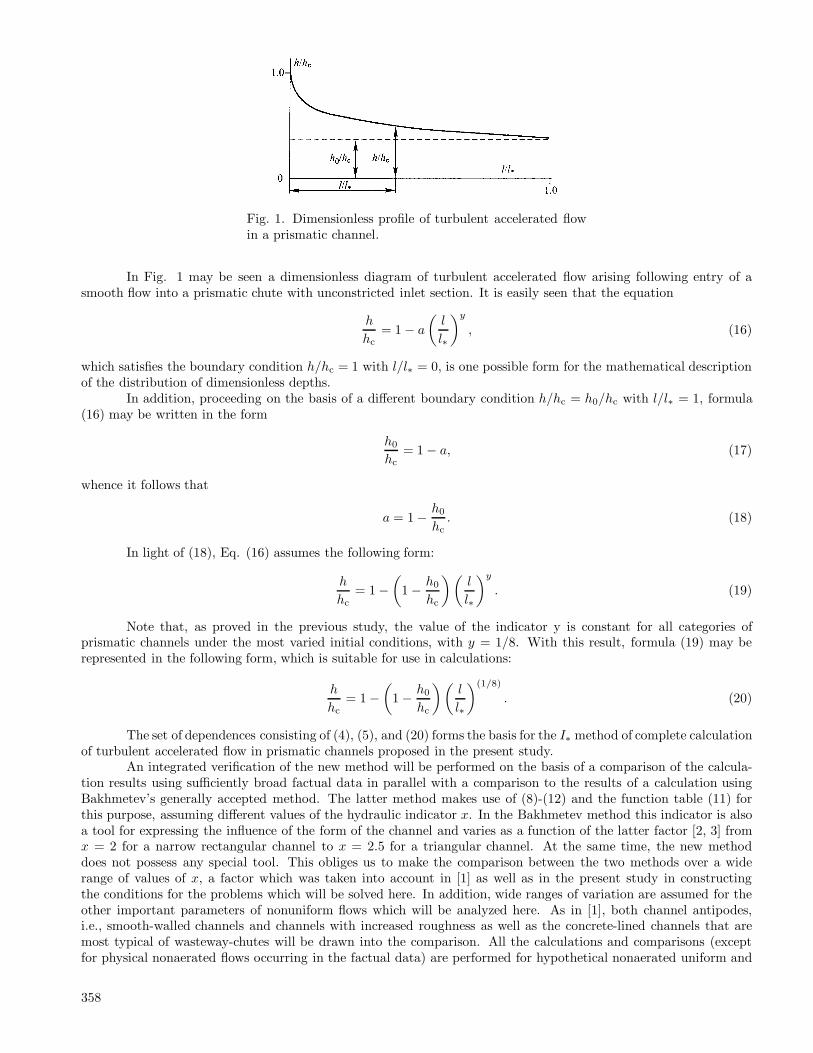
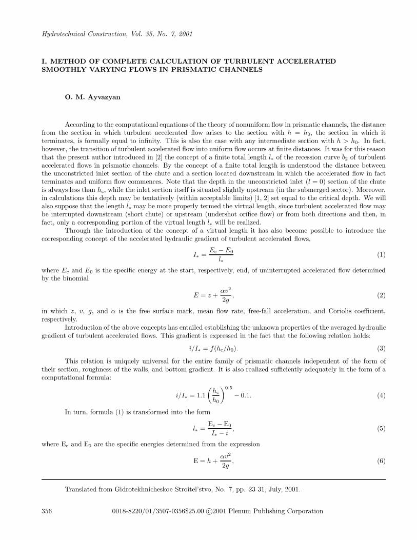
Fig. 1. Dimensionless profile of turbulent accelerated flowin a prismatic channel.

In Fig. 1 may be seen a dimensionless diagram of turbulent accelerated flow arising following entry of asmooth flow into a prismatic chute with unconstricted inlet section. It is easily seen that the equation

h

hc= 1− a

(l

l∗

)y

, (16)

which satisfies the boundary condition h/hc = 1 with l/l∗ = 0, is one possible form for the mathematical descriptionof the distribution of dimensionless depths.

In addition, proceeding on the basis of a different boundary condition h/hc = h0/hc with l/l∗ = 1, formula(16) may be written in the form

h0

hc= 1− a, (17)

whence it follows that

a = 1− h0

hc. (18)

In light of (18), Eq. (16) assumes the following form:

h

hc= 1−

(1− h0

hc

)(l

l∗

)y

. (19)

Note that, as proved in the previous study, the value of the indicator y is constant for all categories ofprismatic channels under the most varied initial conditions, with y = 1/8. With this result, formula (19) may berepresented in the following form, which is suitable for use in calculations:

h

hc= 1−

(1− h0

hc

)(l

l∗

)(1/8)

. (20)

The set of dependences consisting of (4), (5), and (20) forms the basis for the I∗ method of complete calculationof turbulent accelerated flow in prismatic channels proposed in the present study.

An integrated verification of the new method will be performed on the basis of a comparison of the calcula-tion results using sufficiently broad factual data in parallel with a comparison to the results of a calculation usingBakhmetev’s generally accepted method. The latter method makes use of (8)-(12) and the function table (11) forthis purpose, assuming different values of the hydraulic indicator x. In the Bakhmetev method this indicator is alsoa tool for expressing the influence of the form of the channel and varies as a function of the latter factor [2, 3] fromx = 2 for a narrow rectangular channel to x = 2.5 for a triangular channel. At the same time, the new methoddoes not possess any special tool. This obliges us to make the comparison between the two methods over a widerange of values of x, a factor which was taken into account in [1] as well as in the present study in constructingthe conditions for the problems which will be solved here. In addition, wide ranges of variation are assumed for theother important parameters of nonuniform flows which will be analyzed here. As in [1], both channel antipodes,i.e., smooth-walled channels and channels with increased roughness as well as the concrete-lined channels that aremost typical of wasteway-chutes will be drawn into the comparison. All the calculations and comparisons (exceptfor physical nonaerated flows occurring in the factual data) are performed for hypothetical nonaerated uniform and

358

nonuniform flows independently of whether or not they are, in actuality, aerated. Thus, it is necessary to bear inmind that it is precisely the parameters of these hypothetical flows (assuming they are correctly determined) thatbear all of the information about their aerated twins [4, 5].

Before passing on to the results of the calculations and their comparison, let us also present a summary ofother auxiliary dependences that were not used above. The critical depth and uniform flow depth are the same forboth of the methods that are being compared here, and the calculations in both methods begin with these quantities.The critical depth of rectangular sections is determined from the formula

hc =(αQ2

gb2

)1/3

, (21)

while for a triangular section, from the formula,

hc =(2αQ2

gm2

)1/5

, (22)

where b is the bottom width of the channel and m the slope coefficient.Calculations based on the use of (21) and (22), like those based on (6) and (10), were performed with α = 1.1.

The uniform flow depth is determined by a fitting process on the basis of the discharge formula

Q = ωC(Ri)1/2 or Q = ω(8gRiλ

)1/2

. (23)

That the value of h0 thus found is valid is predetermined, while the plausibility of the results of calculationsof nonuniform flow are determined entirely by the validity of the resistance coefficient used in the calculations.

As in [1], proceeding on the basis of the new analysis of the arguments of uniform motion [6] and the resultsof special studies of turbulent nonuniform flows [4, 5, 7], calculations of the resistance coefficient of nonaerated orhypothetical nonaerated flows were performed according to our universal formula

λ = a+ bIx(∆/R)y (24)

in the form of one modification of the latter formula,

λ = a+ k(v0v

)2x

IxRz, (25)

λ = a+ b(ω∆

ω

)y

. (26)

In (24) I , the dimensionless gradient of the specific energy (in the International System of Units), is given by

I =gIR3

v2. (27)

where a, b, x, and y are dimensionless test constants and v is the kinematic viscosity.The first modification (25), in which k is a dimensional test constant (L−z) and z a dimensionless test

constant, the two constants corresponding to the expressions

k = b∆ygxγ−2x0 = const; z = 3x− y = const, (28)

is intended for flows with mixed resistance (to viscosity and roughness) in rigid channels with unknown but constantvalues of the integral parameter ∆ = const and, moreover, constant value of the viscosity v0 = const in tests toestablish the value of k. Since the test values of k that are presented below correspond to v0 ≈ 10−6 m2/s (t0 = 20◦C), in many practically important cases we may set v ≈ v0 in (25), where v is the hypothetical viscosity of the flowthat is being analyzed.

The second modification (26) is intended [5] for calculation of quadratic (x = 0) flows in chutes with increasedroughness in the form of edges of given configuration the height of which ∆ is either specified or must be determined.If the edges extend along the entire perimeter, ω∆/ω = ∆/R. If they are extend along the bed of a rectangularchannel, ω∆/ω = ∆/h, where h and R is the depth and hydraulic radius, respectively, for the wetted cross-sectionat the top of the edges. Below we present the values of the test constants of formulas (25) and (26) for turbulent(Fr > 1) uniform flows for the categories of channels that are considered in the present study:

359

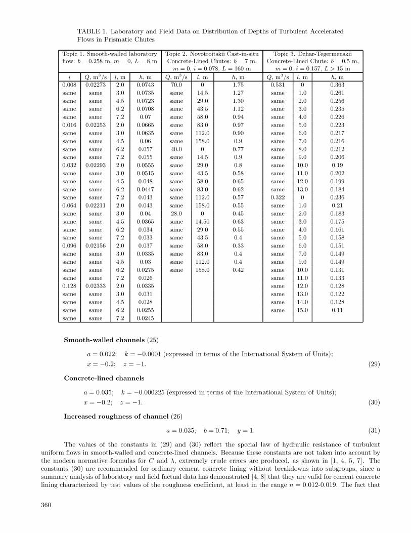
TABLE 1. Laboratory and Field Data on Distribution of Depths of Turbulent AcceleratedFlows in Prismatic Chutes

Topic 1. Smooth-walled laboratory Topic 2. Novotroitskii Cast-in-situ Topic 3. Dzhar-Tegermenskiiflow: b = 0.258 m, m = 0, L = 8 m Concrete-Lined Chutes: b = 7 m, Concrete-Lined Chute: b = 0.5 m,

m = 0, i = 0.078, L = 160 m m = 0, i = 0.157, L > 15 m

i Q, m3/s l, m h, m Q, m3/s l, m h, m Q, m3/s l, m h, m

0.008 0.02273 2.0 0.0743 70.0 0 1.75 0.531 0 0.363

same same 3.0 0.0735 same 14.5 1.27 same 1.0 0.261




0.016 0.02253 2.0 0.0665 same 83.0 0.97 same 5.0 0.223



same same 6.2 0.057 40.0 0 0.77 same 8.0 0.212


0.032 0.02293 2.0 0.0555 same 29.0 0.8 same 10.0 0.19




same same 7.2 0.043 same 112.0 0.57 0.322 0 0.236

0.064 0.02211 2.0 0.043 same 158.0 0.55 same 1.0 0.21

same same 3.0 0.04 28.0 0 0.45 same 2.0 0.183




0.096 0.02156 2.0 0.037 same 58.0 0.33 same 6.0 0.151




same same 7.2 0.026 same 11.0 0.133

0.128 0.02333 2.0 0.0335 same 12.0 0.128

same same 3.0 0.031 same 13.0 0.122

same same 4.5 0.028 same 14.0 0.128

same same 6.2 0.0255 same 15.0 0.11

same same 7.2 0.0245

Smooth-walled channels (25)

a = 0.022; k = −0.0001 (expressed in terms of the International System of Units);x = −0.2; z = −1. (29)

Concrete-lined channels

a = 0.035; k = −0.000225 (expressed in terms of the International System of Units);x = −0.2; z = −1. (30)

Increased roughness of channel (26)

a = 0.035; b = 0.71; y = 1. (31)

The values of the constants in (29) and (30) reflect the special law of hydraulic resistance of turbulentuniform flows in smooth-walled and concrete-lined channels. Because these constants are not taken into account bythe modern normative formulas for C and λ, extremely crude errors are produced, as shown in [1, 4, 5, 7]. Theconstants (30) are recommended for ordinary cement concrete lining without breakdowns into subgroups, since asummary analysis of laboratory and field factual data has demonstrated [4, 8] that they are valid for cement concretelining characterized by test values of the roughness coefficient, at least in the range n = 0.012-0.019. The fact that

360

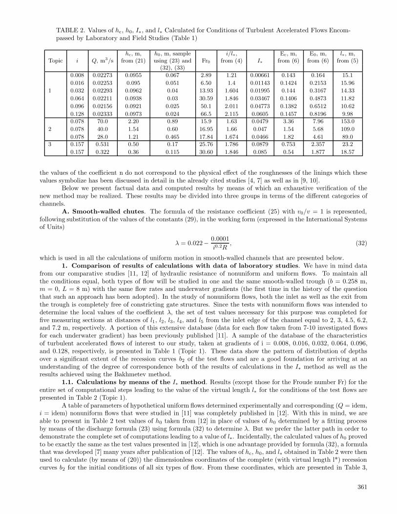
TABLE 2. Values of hc, h0, I∗, and l∗ Calculated for Conditions of Turbulent Accelerated Flows Encom-passed by Laboratory and Field Studies (Table 1)

hc, m, h0, m, sample i/l∗, Ec, m, E0, m, l∗, m,Topic i Q, m3/s from (21) using (23) and Fr0 from (4) I∗ from (6) from (6) from (5)

(32), (33)

0.008 0.02273 0.0955 0.067 2.89 1.21 0.00661 0.143 0.164 15.1

0.016 0.02253 0.095 0.051 6.50 1.4 0.01143 0.1424 0.2153 15.96

1 0.032 0.02293 0.0962 0.04 13.93 1.604 0.01995 0.144 0.3167 14.33

0.064 0.02211 0.0938 0.03 30.59 1.846 0.03467 0.1406 0.4873 11.82

0.096 0.02156 0.0921 0.025 50.1 2.011 0.04773 0.1382 0.6512 10.62

0.128 0.02333 0.0973 0.024 66.5 2.115 0.0605 0.1457 0.8196 9.98

0.078 70.0 2.20 0.89 15.9 1.63 0.0479 3.36 7.96 153.0

2 0.078 40.0 1.54 0.60 16.95 1.66 0.047 1.54 5.68 109.0

0.078 28.0 1.21 0.465 17.84 1.674 0.0466 1.82 4.61 89.0

3 0.157 0.531 0.50 0.17 25.76 1.786 0.0879 0.753 2.357 23.2

0.157 0.322 0.36 0.115 30.60 1.846 0.085 0.54 1.877 18.57

the values of the coefficient n do not correspond to the physical effect of the roughnesses of the linings which thesevalues symbolize has been discussed in detail in the already cited studies [4, 7] as well as in [9, 10].

Below we present factual data and computed results by means of which an exhaustive verification of thenew method may be realized. These results may be divided into three groups in terms of the different categories ofchannels.

A. Smooth-walled chutes. The formula of the resistance coefficient (25) with v0/v = 1 is represented,following substitution of the values of the constants (29), in the working form (expressed in the International Systemsof Units)

λ = 0.022− 0.0001i0.2R

, (32)

which is used in all the calculations of uniform motion in smooth-walled channels that are presented below.1. Comparison of results of calculations with data of laboratory studies. We have in mind data

from our comparative studies [11, 12] of hydraulic resistance of nonuniform and uniform flows. To maintain allthe conditions equal, both types of flow will be studied in one and the same smooth-walled trough (b = 0.258 m,m = 0, L = 8 m) with the same flow rates and underwater gradients (the first time in the history of the questionthat such an approach has been adopted). In the study of nonuniform flows, both the inlet as well as the exit fromthe trough is completely free of constricting gate structures. Since the tests with nonuniform flows was intended todetermine the local values of the coefficient λ, the set of test values necessary for this purpose was completed forfive measuring sections at distances of l1, l2, l3, l4, and l5 from the inlet edge of the channel equal to 2, 3, 4.5, 6.2,and 7.2 m, respectively. A portion of this extensive database (data for each flow taken from 7-10 investigated flowsfor each underwater gradient) has been previously published [11]. A sample of the database of the characteristicsof turbulent accelerated flows of interest to our study, taken at gradients of i = 0.008, 0.016, 0.032, 0.064, 0.096,and 0.128, respectively, is presented in Table 1 (Topic 1). These data show the pattern of distribution of depthsover a significant extent of the recession curves b2 of the test flows and are a good foundation for arriving at anunderstanding of the degree of correspondence both of the results of calculations in the I∗ method as well as theresults achieved using the Bakhmetev method.

1.1. Calculations by means of the I∗ method. Results (except those for the Froude number Fr) for theentire set of computational steps leading to the value of the virtual length l∗ for the conditions of the test flows arepresented in Table 2 (Topic 1).

A table of parameters of hypothetical uniform flows determined experimentally and corresponding (Q = idem,i = idem) nonuniform flows that were studied in [11] was completely published in [12]. With this in mind, we areable to present in Table 2 test values of h0 taken from [12] in place of values of h0 determined by a fitting processby means of the discharge formula (23) using formula (32) to determine λ. But we prefer the latter path in order todemonstrate the complete set of computations leading to a value of l∗. Incidentally, the calculated values of h0 provedto be exactly the same as the test values presented in [12], which is one advantage provided by formula (32), a formulathat was developed [7] many years after publication of [12]. The values of hc, h0, and l∗ obtained in Table 2 were thenused to calculate (by means of (20)) the dimensionless coordinates of the complete (with virtual length l*) recessioncurves b2 for the initial conditions of all six types of flow. From these coordinates, which are presented in Table 3,

361

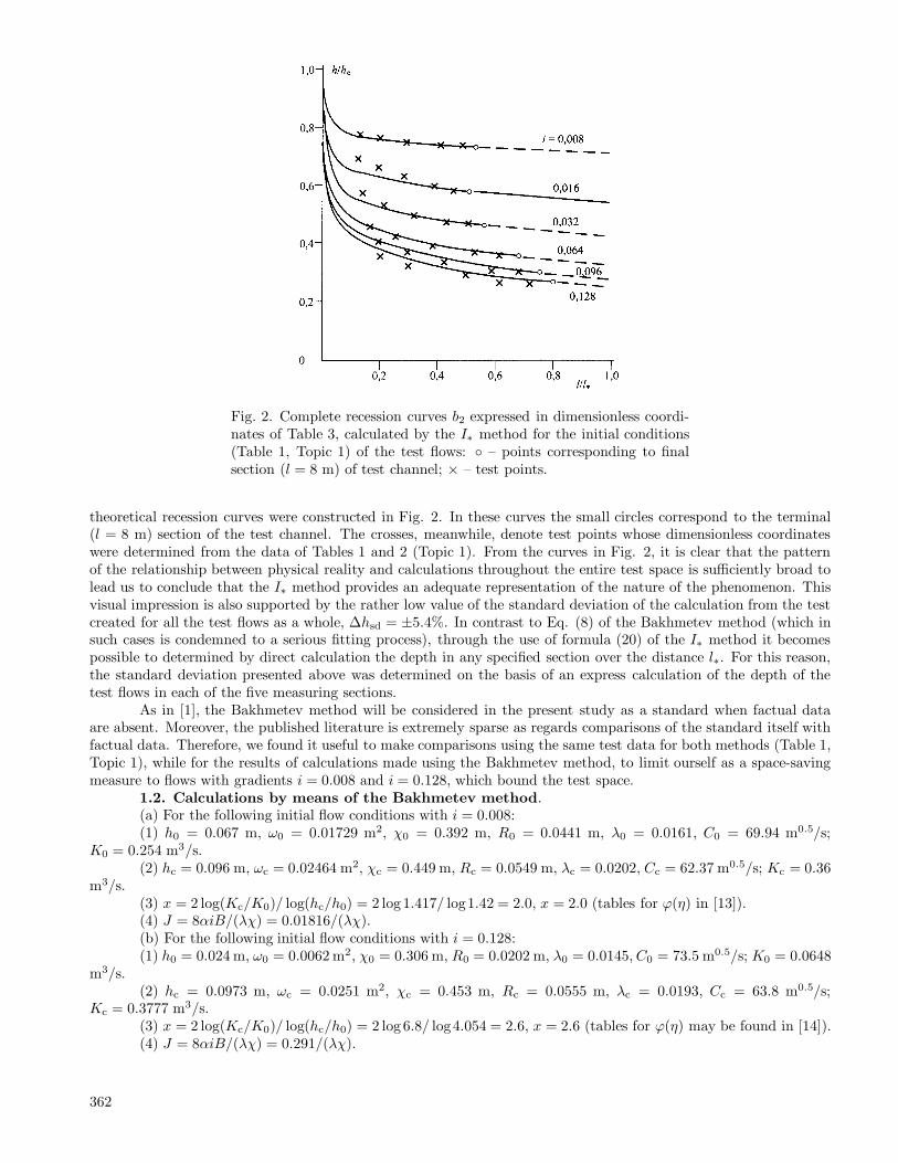
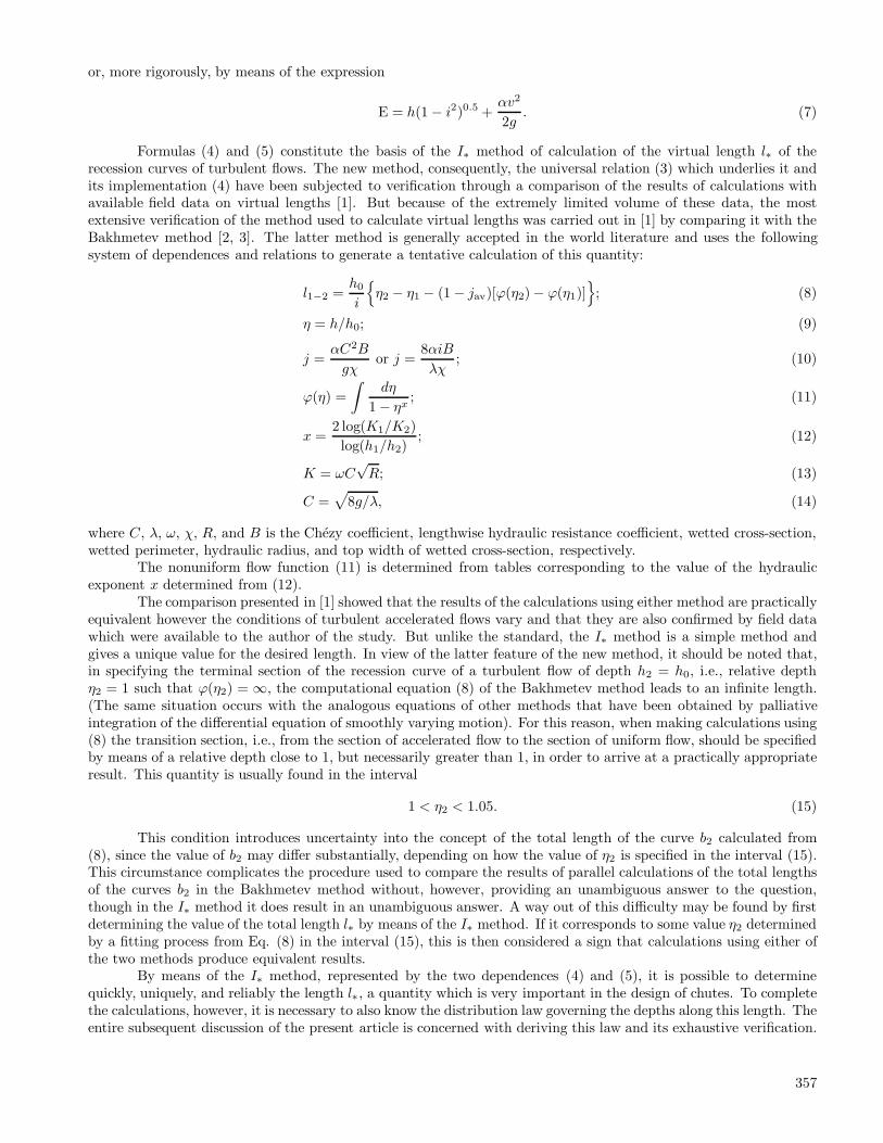
Fig. 2. Complete recession curves b2 expressed in dimensionless coordi-nates of Table 3, calculated by the I∗ method for the initial conditions(Table 1, Topic 1) of the test flows: ◦ – points corresponding to finalsection (l = 8 m) of test channel; × – test points.

theoretical recession curves were constructed in Fig. 2. In these curves the small circles correspond to the terminal(l = 8 m) section of the test channel. The crosses, meanwhile, denote test points whose dimensionless coordinateswere determined from the data of Tables 1 and 2 (Topic 1). From the curves in Fig. 2, it is clear that the patternof the relationship between physical reality and calculations throughout the entire test space is sufficiently broad tolead us to conclude that the I∗ method provides an adequate representation of the nature of the phenomenon. Thisvisual impression is also supported by the rather low value of the standard deviation of the calculation from the testcreated for all the test flows as a whole, ∆hsd = ±5.4%. In contrast to Eq. (8) of the Bakhmetev method (which insuch cases is condemned to a serious fitting process), through the use of formula (20) of the I∗ method it becomespossible to determined by direct calculation the depth in any specified section over the distance l∗. For this reason,the standard deviation presented above was determined on the basis of an express calculation of the depth of thetest flows in each of the five measuring sections.

As in [1], the Bakhmetev method will be considered in the present study as a standard when factual dataare absent. Moreover, the published literature is extremely sparse as regards comparisons of the standard itself withfactual data. Therefore, we found it useful to make comparisons using the same test data for both methods (Table 1,Topic 1), while for the results of calculations made using the Bakhmetev method, to limit ourself as a space-savingmeasure to flows with gradients i = 0.008 and i = 0.128, which bound the test space.

1.2. Calculations by means of the Bakhmetev method.(a) For the following initial flow conditions with i = 0.008:(1) h0 = 0.067 m, ω0 = 0.01729 m2, χ0 = 0.392 m, R0 = 0.0441 m, λ0 = 0.0161, C0 = 69.94 m0.5/s;

K0 = 0.254 m3/s.(2) hc = 0.096 m, ωc = 0.02464 m2, χc = 0.449 m, Rc = 0.0549 m, λc = 0.0202, Cc = 62.37 m0.5/s; Kc = 0.36

m3/s.(3) x = 2 log(Kc/K0)/ log(hc/h0) = 2 log 1.417/ log1.42 = 2.0, x = 2.0 (tables for ϕ(η) in [13]).(4) J = 8αiB/(λχ) = 0.01816/(λχ).(b) For the following initial flow conditions with i = 0.128:(1) h0 = 0.024m, ω0 = 0.0062m2, χ0 = 0.306 m, R0 = 0.0202 m, λ0 = 0.0145,C0 = 73.5 m0.5/s; K0 = 0.0648

m3/s.(2) hc = 0.0973 m, ωc = 0.0251 m2, χc = 0.453 m, Rc = 0.0555 m, λc = 0.0193, Cc = 63.8 m0.5/s;

Kc = 0.3777 m3/s.(3) x = 2 log(Kc/K0)/ log(hc/h0) = 2 log 6.8/ log4.054 = 2.6, x = 2.6 (tables for ϕ(η) may be found in [14]).(4) J = 8αiB/(λχ) = 0.291/(λχ).

362

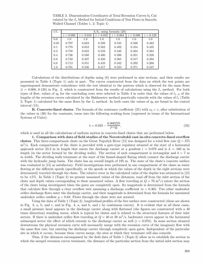
TABLE 3. Dimensionless Coordinates of Total Recession Curves b2 Cal-culated by the I∗ Method for Initial Conditions of Test Flows in Smooth-Walled Channel (Tables 1, 2; Topic 1)

l/l∗ h/hc using formula (20)i = 0.008 i = 0.016 i = 0.032 i = 0.064 i = 0.096 i = 0.128

0.0 1.0 1.0 1.0 1.0 1.0 1.0

0.05 0.797 0.683 0.599 0.535 0.500 0.482

0.1 0.778 0.653 0.562 0.492 0.454 0.435

0.2 0.758 0.622 0.523 0.446 0.404 0.384

0.4 0.736 0.588 0.480 0.396 0.351 0.328

0.6 0.732 0.567 0.450 0.365 0.317 0.294

0.8 0.712 0.551 0.433 0.342 0.292 0.268

1.0 0.701 0.538 0.417 0.323 0.271 0.247

Calculations of the distributions of depths using (8) were performed in nine sections, and their results arepresented in Table 4 (Topic 1) only in part. The curves constructed from the data on which the test points aresuperimposed demonstrate coincidence with the test identical to the pattern which is observed for the same flows(i = 0.008, 0.128) in Fig. 2, which is constructed from the results of calculations using the I∗ method. For bothtypes of flow, values of η9 for the concluding rows were selected in Table 4 in order that the values of l1−9 of thelengths of the recession curves calculated by the Bakhmetev method practically coincide with the values of l∗ (Table2, Topic 1) calculated for the same flows by the I∗ method. In both cases the values of η9 are found in the controlinterval (15).

B. Concrete-lined chutes. The formula of the resistance coefficient (25) with v0 = v, after substitution ofthe values in (30) for the constants, turns into the following working form (expressed in terms of the InternationalSystems of Units):

λ = 0.035− 0.000225i0.2R

, (33)

which is used in all the calculations of uniform motion in concrete-lined chutes that are performed below.1. Comparison with data of field studies of the Novotroitskii cast-in-situ concrete-lined overflow

chutes. This three-compartment chute on the Great Yegorlyk River [15] was designed for a total flow rate Q = 375m3/s. Each compartment of the chute is provided with a gate-type regulator situated at the start of a horizontalapproach sector 23.3 m in length that enters the discharge carrier at a gradient i = 0.078 and is L = 160 m inlength (in the sector formed by the dividing walls). The section of each compartment is rectangular and b = 7 min width. The dividing walls terminate at the start of the funnel-shaped flaring which connect the discharge carrierwith the hydraulic jump basin. The chute has an overall length of 195 m. The state of the chute’s concrete surfacewas evaluated in [15] as satisfactory. Field investigations were performed in one compartment of the chute as waterflowing at the different speeds (specifically, at the speeds at which the values of the depth in the eight sections weredetermined) traveled through the chute. The relative error in the calculated value of the depths was estimated in [15]to be ±5%. In Table 1 (Topic 2) we present measured values of the distances, read off from the inlet section of thechute and depth values corresponding to these measured values. A flow traveling at Q = 70 m3/s enters the sectionof the chute being investigated when the gates are completely open. Its magnitude is determined from the formulathat calculate flow through a clear overflow weir assuming a discharge coefficient m = 0.365. Two other undershotorifice discharge flows enter the discharge carrier, and their magnitude is determined from the formula for unresistedundershot orifice outflow µ = 0.63. Flows through the chute were not aerated.

Using the data of Table 1 (Topic 2), longitudinal profiles of the free surface were constructed (these are shownin Fig. 3, a, b, and c, and in Fig. 4, a, and b, and c by continuous curves). It is evident that in all these cases,a small pressure head appears in the discharge carrier along with flattened (the figures are constructed with a 40times distortion) standing waves, which is typical for chutes and is related to the structural features of their inletsectors. If there is undershot orifice flow traveling at Q = 40 or 28 m3/s, backwater curves appear in the horizontalsubmerged sector the effect of which extends to the discharge carrier as well (i = 0.078). In some section situateddownstream the physical recession curve will necessarily merge with the recession curve of the imaginary flow withthe same flow rate, but entering the discharge carrier through completely open gates. Independent of the particularsite in which it occurs, because these curves merge, the sites at which they terminate will also coincide.

Thus, if the distances encompassed by the field data of Table 1 (Topic 2) allow us to establish the section inwhich the merged recession curves terminate, the distance of the particular section from the initial inlet section may

363

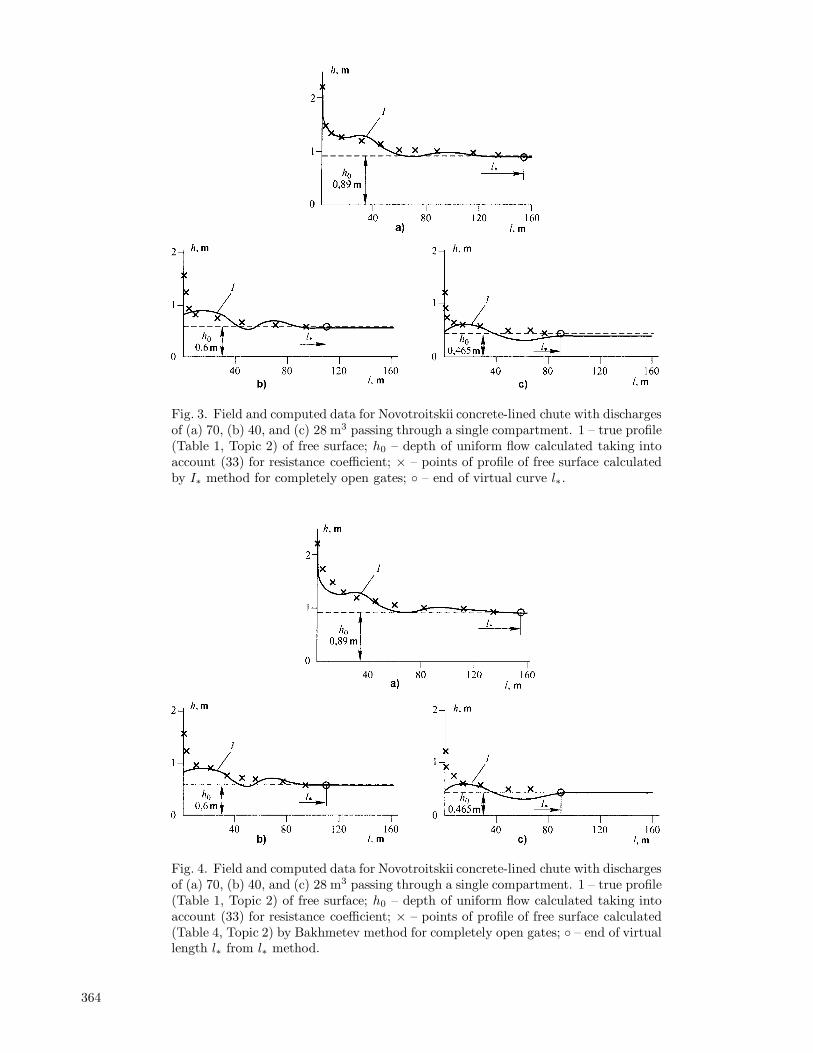
Fig. 3. Field and computed data for Novotroitskii concrete-lined chute with dischargesof (a) 70, (b) 40, and (c) 28 m3 passing through a single compartment. 1 – true profile(Table 1, Topic 2) of free surface; h0 – depth of uniform flow calculated taking intoaccount (33) for resistance coefficient; × – points of profile of free surface calculatedby I∗ method for completely open gates; ◦ – end of virtual curve l∗.

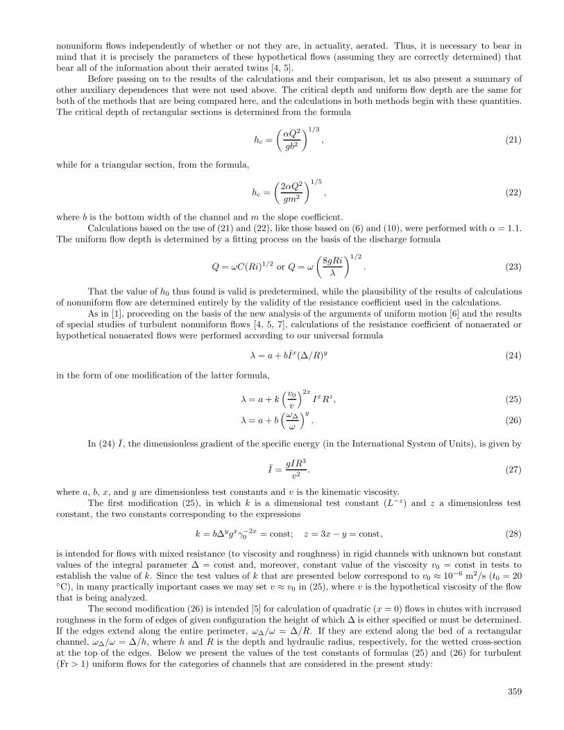
Fig. 4. Field and computed data for Novotroitskii concrete-lined chute with dischargesof (a) 70, (b) 40, and (c) 28 m3 passing through a single compartment. 1 – true profile(Table 1, Topic 2) of free surface; h0 – depth of uniform flow calculated taking intoaccount (33) for resistance coefficient; × – points of profile of free surface calculated(Table 4, Topic 2) by Bakhmetev method for completely open gates; ◦ – end of virtuallength l∗ from l∗ method.

364

TABLE 4. Calculations by the Bakhmetev Method of Complete (within the scope ofthe virtual length l∗) Curves b2 for Physical Conditions (Tables 1, 2; Topics 1, 2, 3) ofInvestigated Flows and for Abstract Conditions in Chute with Increased Roughness

Number of ηN = hN/h0 hN , ϕ(ηN ) R, m λ j jav l1−N

Section from (10)

Topic 1, i = 0.008, Q = 0.02273 m3/s, x = 2.0

1 1.425 0.0955 0.871 0.0549 0.0202 2.00 — 0

2 1.3 0.0871 1.018 0.052 0.017 2.480 2.24 0.480

3 1.2 0.0804 1.199 0.0495 0.017 2.590 2.30 1.690

8 1.02 0.0683 2.307 0.0447 0.0161 2.850 2.43 13.800

9 1.015 0.068 2.415 0.0445 0.0161 2.86 2.43 15.050

Topic 1, i = 0.128, Q = 0.02333 m3/s, x = 2.6

1 4.054 0.0973 0.0677 0.0555 0.0193 33.28 — 0

2 3.000 0.0720 0.1100 0.046 0.0187 38.640 35.96 0.620

3 2.000 0.0480 0.0221 0.035 0.018 46.440 35.86 0.730

8 1.050 0.0252 1.1490 0.0211 0.0148 63.670 48.48 9.080

9 1.038 0.0249 1.26 0.021 0.0148 63.880 48.58 10.040

Topic 2, Q = 70.0 m3/s, x = 2.8

1 2.470 2.2 0.11 1.35 0.0346 12.38 — 0

2 1.97 1.75 0.1744 1.17 0.0346 13.44 12.91 2.68

3 1.65 1.47 0.2510 1.03 0.0346 14.200 13.29 10.04

8 1.035 0.92 1.1360 0.73 0.0346 15.96 14.17 143.60

9 1.025 0.91 1.256 0.72 0.0346 16.000 14.16 155.70

Topic 3, Q = 0.53 m3/s, x = 2.4

1 2.94 0.5 0.1628 0.167 0.0330 13.960 — 0

2 2.00 0.34 0.2920 0.144 0.0327 17.9 15.93 1.068

3 1.75 0.297 0.364 0.136 0.0326 19.37 16.67 2.12

4 1.5 0.255 0.479 0.126 0.0324 21.12 17.54 4.09

9 1.06 0.18 1.252 0.105 0.0319 25.18 19.51 19.74

10 1.04 0.177 1.415 0.104 0.0319 25.36 19.66 23.2

Topic 3, Q = 0.322 m3/s, x = 2.5

1 3.13 0.36 0.1237 0.1480 0.0328 17.27 — 0

2 2.5 0.287 0.1760 0.1340 0.0326 19.73 18.5 0.209

3 2.0 0.230 0.2530 0.1200 0.0323 22.28 19.77 0.945

4 1.8 0.207 0.3030 0.1130 0.0321 23.55 20.41 1.57

9 I.1 0.127 0.9690 0.0840 0.0311 29.44 23.35 12.34

10 1.04 0.12 1.3200 0.0810 0.031 30.14 23.7 18.34

Chute with Increased Roughness (computational problem)B = 0, m = 1.0, l = 0.1 m, i = 0.6, Q = 8.45 m3/s, x = 5.8

1 1.74 1.74 0.0136 0.617 0.150 24.92 0

2 1.5 1.5 0.031 0.532 0.168 22.2 23.56 0.254

3 1.3 1.3 0.066 0.461 0.189 19.79 22.36 1.13

4 1.2 1.2 0.105 0.426 0.202 18.55 21.73 2.25

7 1.01 1.01 0.551 0.358 0.233 16.03 20.47 16.20

8 1.0075 1.0075 0.610 0.357 0.234 16.00 20.46 18.10

be considered the true virtual length l∗ of the recession curve b2 not only in the case Q = 70 m3/s, but also in thecase of undershot orifice discharges traveling at Q = 40 and 28 m3/s.

1.1. Calculations by means of I∗ method. Proceeding on the basis of the above notion, calculations ofturbulent accelerated flows in the Novotroitskii chute were performed for all three discharge rates, under the conditionthat flow enters the discharge carrier when the gates are completely open. In view of the extraordinary (for valuesof h0, hc, and l∗ known from Table 2) simplicity of calculations of the dimensionless coordinates l/l∗ and h/hc ofthe recession curves b2 when performed on the basis of formula (20) of the I∗ method, as shown in Table 3, and thesimplicity of the transition to dimensional coordinates l and h, we will not present tables of the computed values of land h for the three discharge rates of the Novotroitskii chute, limiting ourself to the computed points (small crosses)presented in Fig. 3, a, b, and c. These correspond to the following values of l/l∗: 0, 0.02, 0.06, 0.12, 0.20, 0.30, 0.40,

365

0.50, 0.60, 0.75, 0.90, and 1.0. These points are plotted in Fig. 3, a, b, and c together with the computed (Table 2,Topic 2) depth curve h0 of uniform flow. In the case Q = 70 m3/s (Fig. 3, a), the physical conditions (completelyopen gates) and computation conditions coincide, and the computed points easily fit on the physical curve 1, withthe curve being averaged wherever it is distorted by standing waves. There can be no doubt that the calculationprovides an adequate representation of physical reality throughout the length of the recession curve (except for theprovisional initial section stipulated in advance). Nor can there be any doubt that the physical section in which therecession terminates does, in fact, coincide with the computed section, as determined by the point with coordinatesl∗ and h0. In turn, the combination in Fig. 3, b, c, of the computed points of the free surface b2 of the imagined flows(which arise in the discharge carrier when the gates are completely open) with the curves 1 of the physical undershotorifice flows that previously appears in the discharge carrier confirm the claim that in the latter cases termination ofthe nonuniform regime and the commencement of the uniform regime occurs at the point with computed coordinatesl∗ and h0.

1.2. Calculations by means of the Bakhmetev method. With the same flow rates of Q = 70, 40,and 28 m3/s as above, calculations of accelerated flows b2 by means of the Bakhmetev method were carried out forconditions under which the flow enters the discharge carrier when the gates are completely open. Let us briefly setforth only the results of calculations for the case Q = 70 m3/s. The values of the critical depth hc and depth h0 ofuniform motion, which are the same for the two methods, are taken from Table 2 (Topic 2). Let us next determinethe following additional auxiliary quantities:

(1) h0 = 0.89 m, ω0 = 6.23 m2, χ0 = 8.78 m, R0 = 0.71 m, λ0 = 0.0345, C0 = 47.72 m0.5/s, K0 = 250.6m3/s, hc = 2.2 m, ωc = 15.4 m2, χc = 11.4 m, Rc = 1.35 m, λc = 0.0347, Cc = 47.54 m0.5/s, Kc = 850.6 m3/s.

(2) By (12), x = 2 log(Kc/K0)/ log(hc/h0) = 2.7. (Tables for the closest value x = 2.8 may be found in [2].)(3) By (10), J = 8αiB/(λχ) = 4.8/(λχ).The results of calculations performed on the basis of Eq. (8) for nine gates are presented in part in Table 4

(Topic 2). The value of η9 for the concluding row was selected so that the value of the length l1−9 of the recessioncurve, as calculated by the Bakhmetev method, would practically coincide with the value of the virtual length l∗calculated by the I∗ method. An analogous condition is observed also in the last rows of the table showing calculationsusing Eq. (8) for flow rates Q = 40 and 28 m3/s (these rows are not presented here), however, in all these cases thevalue of η9 turns out to fall within the control interval (15).

Points (×) of the free surface profiles calculated by the Bakhmetev method are constructed on the basis ofthe data of the calculations described above in Fig. 4, a, b, c. The position of these points relative to the factualprofiles I also presented in these figures leads to conclusions analogous to those which were arrived at in the discussionof Fig. 3, a, b, c. But at the same time, the position of the computed points of the I∗ method in relation to thephysical profiles seems more preferable.

2. Comparison with data of field investigations of Dzhar-Tegermenskii concrete-lined overflowchute. Field investigations of the distribution of depths along the Dzhar-Tegermenskii concrete-lined overflow chutewere carried out by the former Central Asia Institute for Water Resources at two flow rates assuming completely opengates in the 15-m initial section (this section is also accessible to measurements). The results of these investigations,which we have borrowed from [16], are presented in Table 1 (Topic 3) with only one correction. In fact, in the tablesof the field data in [16] values of the critical depths that had been calculated using (21) with α = 1.05 were enteredin the inlet section rows (l = 0), though, in fact, the depth in the inlet section is always substantially less than thecritical. Because of this ”row advance,” which is fully in accord with the traditional representation used by mostauthors of textbooks, the depths of 0.363 and 0.236 m that are actually measured in the inlet (l = 0) section weremoved back into the second row of the tables. This error is corrected in the summary Table 1.

2.1. Calculations by means of the I∗ method. We will not present a table showing the calculations ofthe coordinates of the recession curves b2 determined by formula (20) of the I∗ method, in view of the simplicity ofthe operations needed to establish these coordinates following the sample of Table 3 with the addition of a columnof dimensional values. We will limit ourself to giving just the free surface profiles 1 and 2 constructed from the dataof these calculations for both flow rates in the case of the following values of l/l∗: 0, 0.05, 0.10, 0.15, 0.20, 0.30, 0.40,0.50, 0.60, 0.70, 0.95, and 1.0. The test points (Table 1, Topic 3) plotted in Fig. 5, a show that the calculations yieldan entirely adequate representation of the data of the field measurements.

2.2. Calculations by means of the Bakhmetev method. Calculations with Q = 0.531 m3/s. Thevalues of the critical depth and depth of uniform motion, which are the same for both methods, are taken from Table2 (Topic 3). We will now determine the other auxiliary quantities.

(1) h0 = 0.17 m, ω0 = 0.85 m2, χ0 = 0.84 m, R0 = 0.101 m, λ0 = 0.0318, C0 = 49.7 m0.5/s, K0 = 1.342m3/s, hc = 0.5 m, ωc = 0.25 m2, χc = 1.5 m, Rc = 0.167 m, λc = 0.0333, Cc = 48.73 m0.5/s, Kc = 4.98 m3/s.

(2) By (12), x = 2 log(Kc/K0)/ log(hc/h0) = 2.43. (Tables for the closest value x = 2.4 may be found in [2].)(3) By (10), J = 8αiB/(λχ) = 0.691/(λχ).

366

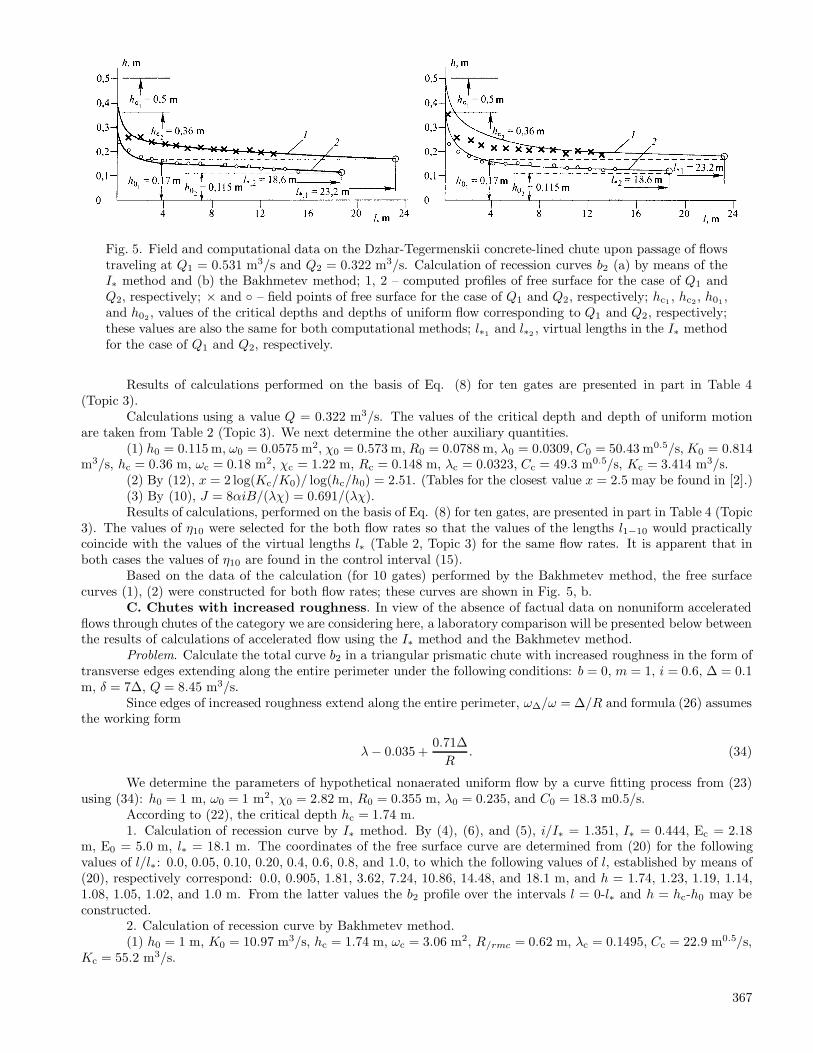
Fig. 5. Field and computational data on the Dzhar-Tegermenskii concrete-lined chute upon passage of flowstraveling at Q1 = 0.531 m3/s and Q2 = 0.322 m3/s. Calculation of recession curves b2 (a) by means of theI∗ method and (b) the Bakhmetev method; 1, 2 – computed profiles of free surface for the case of Q1 andQ2, respectively; × and ◦ – field points of free surface for the case of Q1 and Q2, respectively; hc1 , hc2 , h01 ,and h02 , values of the critical depths and depths of uniform flow corresponding to Q1 and Q2, respectively;these values are also the same for both computational methods; l∗1 and l∗2 , virtual lengths in the I∗ methodfor the case of Q1 and Q2, respectively.

Results of calculations performed on the basis of Eq. (8) for ten gates are presented in part in Table 4(Topic 3).

Calculations using a value Q = 0.322 m3/s. The values of the critical depth and depth of uniform motionare taken from Table 2 (Topic 3). We next determine the other auxiliary quantities.

(1) h0 = 0.115m, ω0 = 0.0575 m2, χ0 = 0.573 m, R0 = 0.0788 m, λ0 = 0.0309, C0 = 50.43 m0.5/s,K0 = 0.814m3/s, hc = 0.36 m, ωc = 0.18 m2, χc = 1.22 m, Rc = 0.148 m, λc = 0.0323, Cc = 49.3 m0.5/s, Kc = 3.414 m3/s.

(2) By (12), x = 2 log(Kc/K0)/ log(hc/h0) = 2.51. (Tables for the closest value x = 2.5 may be found in [2].)(3) By (10), J = 8αiB/(λχ) = 0.691/(λχ).Results of calculations, performed on the basis of Eq. (8) for ten gates, are presented in part in Table 4 (Topic

3). The values of η10 were selected for the both flow rates so that the values of the lengths l1−10 would practicallycoincide with the values of the virtual lengths l∗ (Table 2, Topic 3) for the same flow rates. It is apparent that inboth cases the values of η10 are found in the control interval (15).

Based on the data of the calculation (for 10 gates) performed by the Bakhmetev method, the free surfacecurves (1), (2) were constructed for both flow rates; these curves are shown in Fig. 5, b.

C. Chutes with increased roughness. In view of the absence of factual data on nonuniform acceleratedflows through chutes of the category we are considering here, a laboratory comparison will be presented below betweenthe results of calculations of accelerated flow using the I∗ method and the Bakhmetev method.

Problem. Calculate the total curve b2 in a triangular prismatic chute with increased roughness in the form oftransverse edges extending along the entire perimeter under the following conditions: b = 0, m = 1, i = 0.6, ∆ = 0.1m, δ = 7∆, Q = 8.45 m3/s.

Since edges of increased roughness extend along the entire perimeter, ω∆/ω = ∆/R and formula (26) assumesthe working form

λ− 0.035 +0.71∆R

. (34)

We determine the parameters of hypothetical nonaerated uniform flow by a curve fitting process from (23)using (34): h0 = 1 m, ω0 = 1 m2, χ0 = 2.82 m, R0 = 0.355 m, λ0 = 0.235, and C0 = 18.3 m0.5/s.

According to (22), the critical depth hc = 1.74 m.1. Calculation of recession curve by I∗ method. By (4), (6), and (5), i/I∗ = 1.351, I∗ = 0.444, Ec = 2.18

m, E0 = 5.0 m, l∗ = 18.1 m. The coordinates of the free surface curve are determined from (20) for the followingvalues of l/l∗: 0.0, 0.05, 0.10, 0.20, 0.4, 0.6, 0.8, and 1.0, to which the following values of l, established by means of(20), respectively correspond: 0.0, 0.905, 1.81, 3.62, 7.24, 10.86, 14.48, and 18.1 m, and h = 1.74, 1.23, 1.19, 1.14,1.08, 1.05, 1.02, and 1.0 m. From the latter values the b2 profile over the intervals l = 0-l∗ and h = hc-h0 may beconstructed.

2. Calculation of recession curve by Bakhmetev method.(1) h0 = 1 m, K0 = 10.97 m3/s, hc = 1.74 m, ωc = 3.06 m2, R/rmc = 0.62 m, λc = 0.1495, Cc = 22.9 m0.5/s,

Kc = 55.2 m3/s.

367

(2) By (12), x = 2 log(Kc/K0)/ log(hc/h0) = 5.777. (Tables for the closest value x = 5.8 may be foundin [2].)

(3) By (10), J = 8αiB/(λχ) = 3.74/(λχ).The coordinates of the free surface curve calculated by means of Eq. (8) are presented in part in Table 4.

Values of η8 in the final row are selected so that the distance l1−8 would be precisely equal to the value of the virtuallength l∗, in which case η8 is found in the control interval (15). The combined graph (not presented here) of profilesb2 constructed from the results of calculations based on (20) and from the data of Table 4 (lower part) show that onthe initial third of the virtual length, the Bakhmetev method leads to slightly higher values of the depths than doesthe I∗ method. In view of the fact that this discrepancy is completely identical with the discrepancy found in theBakhmetev method with physical reality (Fig. 4, a), in the present case it may also be interpreted as favoring thenew method.

The above calculations and comparisons for the three categories of channels that have been considered heregraphically show that the results of complete calculations of turbulent accelerated flows carried out using the newmethod provide an adequate representation of the entire volume of factual laboratory and field data which areavailable to the present author, and provide just as adequate a practical representation of the results of calculationsas does the Bakhmetev method for any variations of the initial conditions. Such an assertion is justified by the factthat the present discussion encompasses channels that are antipodes in terms of resistance intensity (λ = 0.0146 andλ = 0.235), in terms of the hydraulic resistance of the channel (x = 2 and 5.8), a factor which reflects the form ofthe channel, and in terms of gradient (i = 0.008 and 0.6).

Conclusions1. A new I∗ method for complete calculation of turbulent accelerated flows b2 has been developed. The

method has been tested over a broad range of initial conditions and has been shown to sufficiently correspond to thefactual data, sometimes exhibiting a higher degree of correspondence than the generally accepted method developedby B. A. Bakhmetev.

2. At the practical level the new method of calculation of flows b2 may be distinguished from Bakhmetev’smethod and other existing methods by its simplicity and universality. There is no requirement for expressly takinginto account the form of the channel or any kind of tabulated functions.

3. At the theoretical level the new method is distinctive in that through its application the problem ofanalyzing flows b2 is solved analytically, avoiding palliative integration of the differential motion equation, a stepthat involves a whole series of frequently arbitrary assumptions, and also bypassing the quite complicated and littlestudied problems of hydraulic resistance of nonuniform flows. This became possible through the use of flows b2,which had been unknown until this property (3) of flows had been discovered. The latter property of flows b2 was, inturn, established [1] through the introduction of concepts of the finite total (virtual) length l∗ and averaged hydraulicgradient I∗ of these flows.

4. The only assumption of the new method involves the determination of the specific energy Ec occurringin (5) from formula (6), which presumes a hydrostatic law of pressure in the discharge section. But the error in thevalue of Ec related to this circumstance cannot be sensitive at low (i > ic) gradients due to the low radii of curvatureof the flow lines. In the case of high (i > ic) gradients, in contrast, it cannot be anticipated that this error will haveany great effect on the results of the calculations due to the weakened role played by Ec itself in the numerator of (5).

5. Note that of the dependences (4), (5) and (20) underlying the I∗ method and the auxiliary dependences(6), (21), (22), and (23), the last four, like (5), are indisputable, while (4) and (20) have been shown to be reliableunder the most varied conditions. In this light, the validity of the process of determining the depth h0 of uniformmotion, which is completely dependent upon the validity of the formula for the resistance coefficient λ of uniformflow, is the only condition to be satisfied in the new method in order to obtain results that provide an adequaterepresentation of physical reality. Thus, we recommend that serious attention be devoted to the set of formulas forλ in the present study and in [1], as well as the results of our studies of uniform flow that have been cited earlier [4,5, 7, 12].

6. The new method of calculating flows b2 with respect to all of the parameters of flows is complete andsuitable for introduction in practical design and operation of chutes used for different purposes.

REFERENCES

1. O. M. Ayvazyan, ”New studies of nonuniform flows: finite total length and averaged hydraulic gradient ofturbulent accelerated flows in prismatic channels,” Gidrotekh. Stroit., No. 7 (1998).

2. B. A. Bakhmetev, Hydraulics of Open Channels [Translated from English], Gosstroiizdat, Moscow-Leningrad,1941.

368

3. R. R. Chugaev, Hydraulics [in Russian], Energoizdat, Leningrad (1982).4. O. M. Ayvazyan, ”Hydraulic resistance and conveyance capacity of uniform turbulent aerated and nonaerated

flows in concrete-lined channels,” Gidrotekh. Stroit., No. 6 (1992).5. O. M. Ayvazyan, ”New studies and a new technique for hydraulic analysis of chutes with increased roughness,”

Gidrotekh. Stroit., No. 6 (1996).6. O. M. Ayvazyan, ”Stability criterion for laminar flow in pipes,” Gidrotekh. Stroit., No. 12 (1985).7. O. M. Ayvazyan, ”Studies of smooth and turbulent flow sin smooth-walled and reinforced iron trough-type

canals,” Gidrotekh. Stroit., No. 2 (1984).8. O. M. Ayvazyan, ”Universal indicator of critical aeration states of uniform and nonuniform smooth and

retarded turbulent flows,” Gidrotekh. Stroit., No. 9 (1994).9. O. M. Ayvazyan, ”Zone of hydraulic resistance in earth canals,” Gidrotekh. Stroit., No. 11 (1987).

10. O. M. Ayvazyan, ”Calculation of conveyance capacity of earth canals and channels,” Gidrotekh. Stroit., No.11 (1989).

11. O. M. Ayvazyan and S. S. Bagdasaryan, ”Comparative study of hydraulic resistances in uniform and nonuni-form smoothly varying motion of open smooth and turbulent flows,” Tr. Koord. Soveshch. po Gidrotekhnike,vyp. 52 (Energiya, Moscow-Leningrad), 1969.

12. O. M. Ayvazyan and S. S. Bagdasaryan, ”Comparative study of hydraulic resistances of smooth and turbu-lent uniform nonaerated flows in a prismatic channel,” Tr. Koord. Soveshch. po Gidrotekhnike, vyp. 52(Energiya, Moscow-Leningrad), 1969.

13. P. G. Kiselev, ed., Handbook on Hydraulic Calculations [in Russian], Energiya, Moscow (1972).14. V. T. Chou, Hydraulics of Open Channels [Russian translation], Izd-vo Lit. po Stroitel’stvo, Moscow (1969).15. I. Kh. Ovcharenko, Studies of Chutes [in Russian], Izv. Vuzov. (1958).16. K. A. Mikhaylov, Irrigation Equipment [in Russian], ONTI, Moscow-Leningrad (1937).

369

i* method of complete calculation of turbulent accelerated smoothly varying flows in prismatic...

Documents