i. introduction - arxiv · pdf fileadditional stimulating factor for pursuing more advanced...
TRANSCRIPT

Post-Newtonian reference-ellipsoid for relativistic geodesy.
Sergei Kopeikin∗Department of Physics & Astronomy, 322 Physics Bldg,
University of Missouri, Columbia, Missouri 65211, USA†
Wenbiao Han‡Shanghai Astronomical Observatory, 80 Nandan Road, Shanghai, 200030, China
Elena Mazurova§Siberian State University of Geosystems and Technologies, Plakhotny St. 10, Novosibirsk 630108, Russia¶
(Dated: January 18, 2016)
We apply general relativity to construct the post-Newtonian background manifold that serves as a referencespacetime in relativistic geodesy for conducting relativistic calculation of the geoid’s undulation and the de-flection of the plumb line from the vertical. We chose an axisymmetric ellipsoidal body made up of perfecthomogeneous fluid uniformly rotating around a fixed axis, as a source generating the reference geometry of thebackground manifold through Einstein’s equations. We, then, reformulate and extend hydrodynamic calcula-tions of rotating fluids done by a number of previous researchers for astrophysical applications to the realm ofrelativistic geodesy to set up algebraic equations defining the shape of the post-Newtonian reference ellipsoid.To complete this task, we explicitly perform all integrals characterizing gravitational field potentials inside thefluid body and represent them in terms of the elementary functions depending on the eccentricity of the ellip-soid. We fully explore the coordinate (gauge) freedom of the equations describing the post-Newtonian ellipsoidand demonstrate that the fractional deviation of the post-Newtonian level surface from the Maclaurin ellipsoidcan be made much smaller than the previously anticipated estimate based on the astrophysical application of thecoordinate gauge advocated by Bardeen and Chandrasekhar. We also derive the gauge-invariant relations of thepost-Newtonian mass and the constant angular velocity of the rotating fluid with the parameters characterizingthe shape of the post-Newtonian ellipsoid including its eccentricity, a semiminor and a semimajor axes. We for-mulate the post-Newtonian theorems of Pizzetti and Clairaut that are used in geodesy to connect the geometricparameters of the reference ellipsoid to the physically measurable force of gravity at the pole and equator of theellipsoid. Finally, we expand the post-Newtonian geodetic equations describing the post-Newtonian ellipsoidto the Taylor series with respect to the eccentricity of the ellipsoid and discuss their practical applications forgeodetic constants and relations adopted in fundamental astronomy.
PACS numbers: 04.20.-q; 04.25.Nx; 91.10.-v; 91.10.By
∗ [email protected]† Also at: Siberian State University of Geosystems and Technologies, Plakhotny St. 10, Novosibirsk 630108, Russia‡ [email protected]§ e [email protected]¶ Also at: Moscow State University of Geodesy and Cartography, 4 Gorokhovsky Alley, Moscow 105064,
Visiting Scholar: Department of Physics & Astronomy, 223 Physics Bldg, University of Missouri, Columbia, Missouri 65211, USA
arX
iv:1
510.
0313
1v2
[gr
-qc]
14
Jan
2016
2
I. INTRODUCTION
Accurate definition, determination and realization of celestial and terrestrial reference frames in the solar system is essentialfor deeper understanding of the underlying principles and concepts of fundamental gravitational physics, astronomy and geo-physics as well as for practical purposes of precise satellite and aircraft navigation, positioning and mapping. It was suggestedlong ago to separate the conceptual meaning of a reference frame and a reference system [1]. The former is understood as a the-oretical construction, including mathematical models and standards for its implementation. The latter is its practical realizationthrough observations and materialization of coordinates of a set of reference benchmarks, e.g., a set of fundamental stars - for theInternational Celestial Reference Frame (ICRF) - or a set of fiducial geodetic stations - for the International Terrestrial ReferenceFrame (ITRF). Continuous monitoring and maintenance of the reference frames and a self-consistent set of geodetic and astro-nomical constants associated with them, is rendered by the International Earth Rotation Service (IERS) and the InternationalUnion of Geodesy and Geophysics (IUGG).
Nowadays, four main geodetic techniques are used to compute accurate terrestrial coordinates and velocities of stations –GPS, VLBI, SLR, and DORIS, for the realizations of ITRF referred to different epochs. The observations are so accuratethat geodesists have to model and to include to the data processing the secular Earth’s crust changes to reach self-consistencybetween various ITRF realizations which are available on http://itrf.ensg.ign.fr/ITRF_solutions/index.php. Thehigher frequencies of the station displacements (mainly due to geophysical phenomena) can be accessed with the formulationspresent in chapter 7 of IERS conventions [2] (see also http://62.161.69.131/iers/convupdt/convupdt.html). Conti-nuity between the ITRF realizations has been ensured when adopting conventions for ICRF and ITRF definitions [2, chapter4]. It is recognized that to maintain the up-to-date ITRF realization as accurate as possible the development of the most precisetheoretical models and parametric relationships is of a paramount importance.
Currently, SLR and GPS allow us to determine the transformation parameters between coordinates and velocities of thecollocation points of the ITRF realizations with the precision of ∼1 mm and ∼1 mm/yr respectively [2, table 4.1]. On the otherhand, the dimensional analysis applied to estimate the relativistic effects in geodesy predicts that the post-Newtonian contributionto the coordinates of the ITRF points on the Earth’s surface (as compared with the Newtonian theory of gravity) is expected to beof the order of the Earth’s gravitational radius that is about 9 mm [3, 4] or, may be, less [5]. This post-Newtonian geodetic effectemerges as an irremovable long-wave deformation of the three-dimensional coordinate grid of ITRF which might be potentiallymeasurable with the currently available geodetic techniques and, hence, deserves to be taken into account when building theITRF realization of a next generation.
ITRF solutions are specified by the Cartesian equatorial coordinates xi = x, y, z of the reference geodetic stations. For thepurposes of geodesy and gravimetry the Cartesian coordinates are often converted to geographical coordinates h, θ, λ (h - height,θ - latitude, λ - longitude) referred to an international reference ellipsoid which is a solution found by Maclaurin [6] for the figureof a fluid body with a homogeneous mass density that slowly rotates around a fixed z-axis with a constant angular velocity ω. Forthe post-Newtonian effects deforms the shape of the reference-ellipsoid [7, 8] and modify the basic equations of classic geodesy[9, 10], they must be properly calculated to ensure the adequacy of the geodetic coordinate transformations at the millimeterlevel of accuracy. In order to evaluate more precisely the post-Newtonian effects in the shape of the Earth’s reference ellipsoidand the geodetic equations we have decided to conduct more precise mathematical study of equations of relativistic geodesywhich is given in the present paper.
Certainly, we are touching upon the topic which has been already discussed in literature by research teams from USA [7, 8, 11–18], Lithuania [19–21], USSR [22–25] and, the most recently, by theorists from the University of Jena in Germany [26–30]. Wedraw attention of the reader that the previous papers focused primarily on studying the astrophysical aspects of the problemlike the instability of the equilibrium rotating configurations and the points of bifurcations, finding exact solutions of Einstein’sequations for axially-symmetric spacetimes, emission of gravitational waves, etc. Our treatment concerns different aspectsand is focused on the post-Newtonian effects in physical geodesy. More specifically, we extend the research on the figures ofequilibrium into the realm of relativistic geodesy and pay attention mostly to the possible geodetic applications for an adequatenumerical processing of the high-precise data obtained by various geodetic techniques that include but not limited to SLR, LLR,VLBI, DORIS and GNSS [31, 32]. This vitally important branch of the theory of equilibrium of rotating bodies was not coveredby the above-referenced astrophysical works.
Additional stimulating factor for pursuing more advanced research on relativistic geodesy and the Earth figure of equilibriumis related to the recent breakthrough in manufacturing quantum clocks [33], ultra-precise time-scale dissemination over theglobe [34], and geophysical applications of the clocks [35, 36]. Clocks at rest in a gravitational potential tick slower than clocksoutside of it. On Earth, this translates to a relative frequency change of 10−16 per meter of height difference [37]. Comparing thefrequency of a probe clock with a reference clock provides a direct measure of the gravity potential difference between the twoclocks. This novel technique has been dubbed chronometric levelling. It is envisioned as one of the most promising applicationof the relativistic geodesy in a near future [10, 38, 39]. Optical frequency standards have recently reached stability of 2.2×10⁻¹⁶
at 1 s, and demonstrated an overall fractional frequency uncertainty of 2.1 × 10⁻¹⁸ [40] which enables their use for relativisticgeodesy at an absolute level of one centimetre.
The chronometric levelling directly measures the equipotential surface of gravity field (geoid) without conducting a compli-

3
cated gravimetric survey and solving the differential equations for anomalous gravity potentials [39]. Combining the data ofthe chronometric levelling with those of the conventional geodetic techniques will allow us to determine the normal heightsof reference points with an unprecedented accuracy [35]. An adequate physical interpretation of this type of measurements isinconceivable without an accompanying development of the corresponding mathematical algorithms accounting for the majorrelativistic effects in geodesy.
Basic theoretical concepts of relativistic geodesy have been discussed in a number of textbooks, most notably [9, 41–43] andreview papers [5, 10, 39]. Nonetheless, theoretical problem of the determination of the reference level surface in relativisticgeodesy has not yet been discussed in scientific literature with a full mathematical rigour. The objective of the present paper isto give its comprehensive post-Newtonian solution. To this end, section II explains briefly the principles of the post-Newtonianapproximations and describes the post-Newtonian metric tensor. Section III discusses the post-Newtonian ellipsoid which gen-eralizes the Maclaurin ellipsoid and is the surface of the fourth order. Section IV introduces the reader to the concept of thepost-Newtonian gauge freedom and shows how this freedom can be used to simplify the mathematical description of the PN el-lipsoid. Sections V and VI calculate respectively the Newtonian and post-Newtonian gravitational potentials inside the rotatingPN ellipsoid. Section VII gives the post-Newtonian definitions of the conserved mass and angular momentum of the rotatingPN ellipsoid. Section VIII is devoted to the derivation of the post-Newtonian equations defining the geometric structure of thereference level surface and its kinematic relation to the angular velocity of rotation ω. Sections IX and X provide the reader withthe relativistic generalization of the Pizzetti and Clairaut theorem of classical geodesy [44, 45] which connect parameters of thereference ellipsoid with the measured value of the force of gravity. Finally, section XI gives truncated versions of the relativisticformulas which can be used in practical applications of relativistic geodesy. Appendix A contains details of the mathematicalcalculation of integrals.
We adopt the following notations:
• the Greek indices α, β, ... run from 0 to 3,
• the Roman indices i, j, ... run from 1 to 3,
• repeated Greek indices mean Einstein’s summation from 0 to 3,
• repeated Roman indices mean Einstein’s summation from 1 to 3,
• the unit matrix (also known as the Kroneker symbol) is denoted by δi j = δi j,
• the fully antisymmetric symbol Levi-Civita is denoted as εi jk = εi jk with ε123 = +1,
• the bold letters a = (a1, a2, a3) ≡ (ai), b = (b1, b2, b3) ≡ (bi), and so on, denote spatial 3-dimensional vectors,
• a dot between two spatial vectors, for example a · b = a1b1 + a2b2 + a3b3 = δi jaib j, means the Euclidean dot product,
• the cross between two vectors, for example (a × b)i ≡ εi jka jbk, means the Euclidean cross product,
• we use a shorthand notation for partial derivatives ∂α = ∂/∂xα,
• gαβ is the spacetime metric,
• the Greek indices are raised and lowered with the metric gαβ,
• the Minkowski (flat) space-time metric ηαβ = diag(−1,+1,+1,+1), it is used to rise and lower indices of the gravitationalmetric perturbation, hαβ.
• G is the universal gravitational constant,
• c is the speed of light in vacuum,
• ω is a constant rotational velocity of the Earth,
• ρ is a constant density of reference-ellipsoid,
• a is a semimajor axis of the Maclaurin ellipsoid,
• b is a semiminor axis of the Maclaurin ellipsoid,
• κ ≡ πGρa2/c2 is a dimensional parameter characterizing the strength of gravitational field,
• R⊕ is the mean (volumetric) radius of the Earth, R⊕ ' 6.3710 × 108 cm,
• a⊕ is the equatorial radius of the Earth reference ellipsoid, a⊕ ' 6.3781 × 108 cm,
• b⊕ is the polar radius of the Earth reference ellipsoid, b⊕ ' 6.3568 × 108 cm.
Other notations are explained in the text as they appear.
4
II. POST-NEWTONIAN METRIC
Einstein’s field equations represent a system of ten non-linear differential equations in partial derivatives for the metric tensor,gαβ, and we have to find their solutions for the case of an isolated rotating fluid. Because the equations are difficult to solveexactly due to their non-linearity, we apply the post-Newtonian approximations (PNA) for their solution [7].
The PNA are applied in case of slowly-moving matter having a weak gravitational field. This is exactly the situation in thesolar system which makes PNA highly appropriate for constructing a relativistic theory of reference frames [46] and relativisticcelestial mechanics in the solar system [9, 41, 47].
The PNA are based on the assumption that a Taylor expansion of the metric tensor can be done in inverse powers of thefundamental speed c that is equal to the speed of light in vacuum. Exact mathematical formulation of a set of basic axiomsrequired for doing the post-Newtonian expansion was given by Rendall [48]. Practically, it requires to have several smallparameters characterizing the source of gravity. They are: εi ∼ vi/c, εe ∼ ve/c, and ηi ∼ Ui/c2, ηe ∼ Ue/c2, where vi is acharacteristic velocity of motion of matter inside a body, ve is a characteristic velocity of the relative motion of the bodies withrespect to each other, Ui is the internal gravitational potential of each body, and Ue is the external gravitational potential betweenthe bodies. If one denotes a characteristic radius of a body as L and a characteristic distance between the bodies as R, the internaland external gravitational potentials will be Ui ' GM/L and Ue ' GM/R, where M is a characteristic mass of the body. Dueto the virial theorem of the Newtonian gravity [7] the small parameters are not independent. Specifically, one has ε2
i ∼ ηi andε2
e ∼ ηe. Hence, parameters εi and εe are sufficient in doing post-Newtonian approximations. Because within the solar systemthese parameters do not significantly differ from each other, they will be not distinguished when doing the post-Newtonianiterations. In particular, notation ε ≡ 1/c is used to mark the powers of the fundamental speed c in the post-Newtonian terms.This parameter is also considered as a primary parameter of the PNA scheme to each all the other parameters are approximatelyequal, for example, εi = εvi, ηi = ε2Ui, etc.
We work in the framework of general relativity and adopt the harmonic coordinates xα = (x0, xi), where x0 = ct, and t is thecoordinate time. The class of the harmonic coordinates is defined by imposing the de Donder gauge condition on the metrictensor [49, 50],
∂α(√−ggαβ
)= 0 . (1)
Our choice of the harmonic coordinates is not of the principal value. Calculations could be performed in arbitrary coordinates.Nonetheless the choice of the harmonic coordinates is dictated by their long-term use in relativistic celestial mechanics, astrom-etry and geodesy [4, 9, 47, 51]. Furthermore, all relativistic algorithms of the data processing of high-precise astronomical andgeodetic observations are written down in harmonic coordinates and are recommended to use by the International AstronomicalUnion (IAU) resolutions [2, 46]
Einstein equations for the metric tensor are a complicated non-linear system of differential equations in partial derivatives.Because gravitational field of the solar system is weak and motion of matter is slow, we can focus on the first post-Newtonianapproximation of general relativity. Furthermore, we assume that Earth rotates uniformly with angular velocity ω around a fixedaxis which we identify with z-axis. We shall also neglect tides, and consider Earth as an isolated body. Under these assumptionsthe spacetime becomes stationary with the post-Newtonian metric having the following form [9]
g00 = −1 +2Vc2 +
2c4
(Φ − V2
)+ O
(c−6
), (2)
g0i = −4V i
c3 + O(c−5
), (3)
gi j = δi j
(1 +
2Vc2
)+ O
(c−4
), (4)
where the gravitational potentials entering the metric, satisfy the Poisson equations,
∆V = −4πGρ , (5)∆V i = −4πGρvi , (6)
∆Φ = −4πGρ(2v2 + 2V + Π +
3pε
), (7)
with p and vi being pressure and velocity of matter respectively, and Π is the internal energy of matter per unit mass. We empha-size that ρ is the local mass density of baryons per a unit of invariant (3-dimensional) volume element dV =
√−gu0d3x, where
u0 is the time component of the 4-velocity of matter. The local mass density, ρ, relates in the post-Newtonian approximation tothe invariant mass density ρ∗ =
√−gu0ρ. In the first post-Newtonian approximation this equation reads
ρ∗ = ρ +ρ
c2
(12
v2 + 3V). (8)

5
We assume that the matter consists of a perfect fluid. Then, the internal energy, Π, is related to pressure, p, and the local density,ρ, by thermodynamic equation
dΠ + pd(
1ρ
)= 0 , (9)
and the equation of state, p = p(ρ). In the present paper we consider the case of a body consisting of a fluid with a constant massdensity ρ = const. Equation (9) states then, that inside such a fluid the internal energy Π is also constant.
In the stationary spacetime, the mass density ρ∗ obeys the exact equation of continuity
∂i
(ρ∗vi
)= 0 . (10)
Velocity of rigidly rotating fluid is
vi = εi jkω jxk , (11)
where ωi is the constant angular velocity. Replacing velocity vi in (10) with (11), and differentiating, reveals that
vi∂iρ = 0 , (12)
which means that velocity of the fluid is tangent to the surfaces of constant density ρ.Modelling the real Earth as a rotating fluid ball of constant density is, of course, unrealistic from geophysical point of view as
it is inconsistent neither with the seismological data [52] nor with IERS data on the Earth’s rotation which clearly indicates thepresence of the several layers of different density. Nonetheless, when one considers the geodetic problem of the terrestrial refer-ence frame the realistic model of the Earth’s interior leads to enormous practical difficulties in establishing the geoid’s surface.Indeed, calculation of the geoid requires a well-defined reference level surface occupied by rotating fluid and approximating thegeoid with the height’s deviations as minimal as possible. If one takes a realistic mass distribution the reference level surfacecan not be an ellipsoid of rotation [53]. Furthermore, the gravity field of such a figure of equilibrium (so-called, normal gravityfield [54]) will be described by too complicated mathematical equations which are not suitable for practical applications. Acompromise is to take the reference level of the rotating fluid body as an ellipsoid which allows us to derive the normal gravityfield in a concise meaningful form. However, such a reference ellipsoid of rotation can be maintained only by a homogeneousdensity distribution [53]. Fortunately, the maximum deviation between the level surfaces of the realistic density distribution andthe surfaces of equal density are of the order of e2 ' 1/298 only, and the differences in stress at the model remain considerablysmaller than in the real Earth [43, 55]. This explains why the classic geodesy operates with the reference Maclaurin ellipsoid ofconstant density as a reference surface.
The same reasons are applied for justification of using the constant density ρ to build the reference level surface in relativisticgeodesy. The constant density allows us to solve the post-Newtonian equations exactly so that we can write down precisemathematical equations to describe the gravitational field of the post-Newtonian rotating fluid configuration. However, as weshall see in the next section, the rotating fluid of constant density cannot be an ellipsoid of revolution in the post-Newtonianapproximation but a surface of the fourth order. In the post-Newtonian approximation it is possible to build the rotating ellipsoidof revolution which is a surface of the second order, only under assumption that the density of the fluid has an inhomogeneousellipsoidal distribution of mass [56]. The deviation from the inhomogeneity are of the post-Newtonian order of magnitude,δρ/ρ ' GM⊕/c2R⊕ ' 7×10⁻¹⁰, and are practically unmeasurable in local experiments. Nonetheless, the relativistic effects in thenormal gravity field produced by such a density inhomogeneity over the global scale might be noticed in precise measurementsof the gravity field conducted with the next generation of gravimeters [57, 58] and/or gravity gradientometers [59–61]. Thus, weagain has to compromise between two models of the Earth’s interior - a non-homogeneous density distribution of matter inside areference level ellipsoid or a homogeneous density with the small, post-Newtonian deviations of the reference level surface fromthe precise ellipsoid of revolution. It is not the goal of the present paper to decide between the two cases. Instead, we focus onthe solution of the problem of the rotating fluid having a homogeneous distribution of density as the most tractable mathematicalcase extrapolating the Newtonian case of the Maclaurin ellipsoid to relativistic geodesy. The case of the inhomogeneous densitydistribution and comparison with the homogeneous density model will be considered somewhere else.
III. POST-NEWTONIAN REFERENCE-ELLIPSOID
In classical geodesy the reference figure for calculation of geoid’s undulation is the Maclaurin ellipsoid of a rigidly rotatingfluid of a constant density ρ. Maclaurin’s ellipsoid is a surface described by a polynomial of the second order [53]
x2 + y2
a2 +z2
b2 = 1 , (13)

6
where a and b are semimajor and semiminor axes of the ellipsoid. This property is because the differential Euler equation definingthe equilibrium of gravity and pressure is of the first order partial differential equation which first integral is the Newtoniangravity potential that is a scalar function represented by a polynomial of the second order with respect to the Cartesian spatialcoordinates. In what follows, we assume a > b, and define the eccentricity of the Maclaurin ellipsoid by a standard formula[43, 54]
e ≡
√a2 − b2
a2 . (14)
We shall demonstrate in the following sections that in the post-Newtonian approximation the gravity potential, W, of therotating homogeneous fluid is a polynomial of the fourth order as was first noticed by Chandrasekhar [7]. Hence, the levelsurface of a rigidly-rotating fluid is expected to be a surface of the fourth order. We shall assume that the surface remainsaxisymmetric in the post-Newtonian approximation and dubbed the body with such a surface as a PN ellipsoid [62].
We shall denote all quantities taken on the surface of the PN ellipsoid with a bar to distinguish them from the coordinatesoutside of the surface. Let the barred coordinates xi = x, y, z denote a point on the surface of the PN ellipsoid with the axis ofsymmetry directed along the rotational axis and with the origin located at its post-Newtonian center of mass. Post-Newtoniandefinitions of mass, the center of mass, and the other multipole moments of an extended astronomical body can be found, forexample, in [9, chapter 4.5.3] and are also given in section VII of the present paper. Let the rotational axis coincide with thedirection of z axis. Then, the most general equation of the PN ellipsoid is
σ2
a2 +z2
b2 = 1 + κF(x) , (15)
where σ2 ≡ x2 + y2, κ ≡ πGρa2/c2 is the post-Newtonian parameter which is convenient in the calculations that follow,
F(x) ≡ K1σ2
a2 + K2z2
b2 + E1σ4
a4 + E2z4
b4 + E3σ2z2
a2b2 , (16)
and K1,K2, Ei (i = 1, 2, 3) are arbitrary numerical coefficients.Let xi = x, y, z be any point inside the PN ellipsoid. We introduce a quadratic polynomial
C(x) ≡σ2
a2 +z2
b2 − 1 , (17)
where σ2 ≡ x2 + y2. This polynomial vanishes on the boundary surface of the Maclaurin ellipsoid (13). However, in thepost-Newtonian approximation we have on the boundary of the PN ellipsoid (15) the following condition
C(x) = κF(x) . (18)
In terms of the polynomial C(x) function F(x) in the right-hand side of (15) can be formally recast to
F(x) = K1 + E1 − (K1 − K2 + 2E1 − E3)z2
b2 + (E1 + E2 − E3)z4
b4 + R(x) , (19)
where the reminder
R(x) ≡[K1 + E1 + E1
σ2
a2 + (E3 − E1)z2
b2
]C(x) . (20)
The remainder R(x) can be discarded on the boundary of the PN ellipsoid because R(x) = 0. This property indicates a specificfreedom in the definition of the surface of the PN ellipsoid. Namely, equation (15) is defined up to a class of equivalence modulofunction C(x) given in (17) that vanishes on the surface of the Maclaurin ellipsoid, C(x) = 0. It means that the surface of the PN
ellipsoid defined by equation (15) is always determined in the post-Newtonian terms only up to a function(α1σ2
a2 + α2z2
b2
)C(x)
where α1, α2 are arbitrary constant parameters. By making a specific choice of the parameters α1, α2 we can eliminate any twoof the five coefficients K1,K2, E1, E2, E3 entering function F(x) in (15). It is convenient to chose K1 = K2 = 0 that simplifiesthe equations which follow. The choice K1 = K2 = 0 is equivalent to rescaling the semimajor and semiminor axes, a and b, in(15) respectively.
Each cross-section of the PN ellipsoid being orthogonal to the rotational axis, represents a circle. The equatorial cross-sectionhas an equatorial radius, σ = re, being determined from (15) by the condition z = 0. It yields
re = a(1 +
12κE1
). (21)

7
𝜃 𝑥
𝑧
𝑟𝑒
𝑟𝑝
𝜑 𝜃 𝑥
𝑧
𝑎
𝑏
𝜑
FIG. 1. Meridional cross-section of the PN ellipsoid (a red curve in the on-line version) versus the Maclaurin ellipsoid (a blue curve in theon-line version). The left panel represents the most general case with arbitrary values of the shape parameters E1, E2, E3 when the equatorial,re, and polar, rp, radii of the PN ellipsoid differ from the semimajor, a, and semiminor, b, axes of the Maclaurin ellipsoid, re , a, rp , b. Theright panel shows the case of E1 = E2 = 0 when the equatorial and polar radii of the PN ellipsoid and the Maclaurin ellipsoid are equal. Theangle ϕ is the geographic latitude (−90 ≤ ϕ ≤ 90), and the angle θ is a complementary angle (co-latitude) used for calculation of integralsin appendix of the present paper (0 ≤ θ ≤ π). In general, when E1 , E2 , 0, the maximal radial difference (the ’height’ difference) betweenthe surfaces of the PN ellipsoid and the Maclaurin ellipsoid depends on the choice of the post-Newtonian coordinates, and can amount to afew cm. Carefully operating with the residual gauge freedom of the post-Newtonian theory by choosing E1 = E2 = 0, allows us to make thedifference between the two surfaces much less than one millimeter that is practically unobservable at the present time (for more discussion seesection XI).
The meridional cross-section of the PN ellipsoid is no longer an ellipse (as it was in case of the Maclaurin ellipsoid) but a curveof the fourth order. Nonetheless, we can define the polar radius, z = rp, of the PN ellipsoid by the condition, σ = 0. Equation(15) yields
rp = b(1 +
12κE2
). (22)
In terms of the parameters re and rp equation (15) of the PN ellipsoid takes on the following form
σ2
r2e
+z2
r2p
= 1 − κ (E1 + E2 − E3) z2
r2p−
z4
r4p
. (23)
This reveals that only a single combination, E1 + E2 − E3, of the parameters explicitly appears in the description of the shape ofthe PN ellipsoid in the harmonic coordinates while the other two parameters, E1 and E2, can be absorbed (like the coefficientsK1 and K2 above) to its equatorial and polar radii. The combination E1 + E2 − E3 is determined by the physical equation of theequilibrium of the rotating fluid as explained in section VIII. Parameters E1 and E2 are not limited by physics and can be chosenarbitrary within the accuracy allowed by the post-Newtonian approximation. We discuss their possible choice in sections VIIIand XI.
We characterize the ‘oblateness’ of the PN ellipsoid (23) by the post-Newtonian ‘eccentricity’
ε ≡
√r2
e − r2p
re. (24)
It differs from the eccentricity (14) of the Maclaurin ellipsoid by relativistic correction
ε = e − κ1 − e2
2e(E2 − E1) . (25)
In case, when either E2 = E1 or E1 = E2 = 0, the two eccentricities coincide. The possible configurations of the PN ellipsoidversus Maclaurin’s ellipsoid are visualized in Fig. 1.

8
IV. POST-NEWTONIAN GAUGE FREEDOM
Theoretical formalism for calculation of the post-Newtonian level surface can be worked out in arbitrary coordinates. Formathematical and historic reasons the most convenient are harmonic coordinates which are also used by the IAU [46] and IERS[2] astro-geodetic data processing centers. The harmonic coordinates are selected by the de Donder condition (1) but it does notpick up a single coordinate system because of the property known as a residual gauge freedom [63]. It means that the gaugecondition (1) selects an infinite set of harmonic coordinates interrelating by coordinate transformations which don’t violatethe gauge condition (1). The field equations (5)–(7) and their solutions are form-invariant with respect to the residual gaugetransformations. The residual gauge freedom can be further limited by imposing additional constraints on the metric tensor [9].
The residual gauge freedom of the harmonic coordinates is described by a post-Newtonian coordinate transformation,
x′α = xα + κξα(x) , (26)
where functions, ξα, obey the Laplace equation [63],
∆ξα = 0 . (27)
We discuss the case of the solution of the post-Newtonian equations (5)–(7) inside the rotating fluid. Therefore, the solution ofthe Laplace equation (27) must be convergent at the origin of the coordinate system. It is well known that such a solution is givenin terms of the harmonic polynomials which are selected by the condition that the shape of the PN ellipsoid given by equation15 remains the polynomial of the fourth order with the rotational symmetry about z-axis. This condition reduces the functionsξα in (26) to the harmonic polynomials of the third order having the following form
ξ1 = hx +pxa2
(σ2 − 4z2
), (28a)
ξ2 = hy +pya2
(σ2 − 4z2
), (28b)
ξ3 = kz +qzb2
(3σ2 − 2z2
), (28c)
where h, k, p and q are arbitrary constant parameters. It can be checked by direct inspection that the polynomials (28a)–(28c)satisfy the Laplace equation (27). We have chosen, ξ0 = 0, because we consider a stationary spacetime which means thatall functions are time-independent. We emphasize that the transformation (28a)–(28c) does not preserve the element of thecoordinate volume d3x in the most general case. The coordinate volume would be preserved if ∂αξα = 0 that implies k = −2hand q = −4b2 p/3a2. This constraint on the gauge transformation was originally employed by Chandrasekhar [11] who treatedthe volume-preserved transformations as the Lagrange displacements of the Maclaurin ellipsoid. Later on, Chandrasekharabandoned this constraint [14] to adjust his theory to physical criteria for comparison of the post-Newtonian and Newtonianconfigurations of rotating fluids proposed by Bardeen [8] (see section VIII for further detail).
Coordinate transformation (26) with ξi taken from (28a)–(28c) does not violate the harmonic gauge condition (1) but it changesequations (15) and (16) to
σ′2
a2 +z′2
b2 = 1 + κF′(x′) , (29)
F′(x′) ≡ K′1σ′2
a2 + K′2z′2
b2 + E′1σ′4
a4 + E′2z′4
b4 + E′3σ′2z′2
a2b2 , (30)
where σ′2 ≡ x′2 + y′2, and the primed coefficients are
K′1 = K1 + 2h , (31a)K′2 = K2 + 2k , (31b)E′1 = E1 + 2p , (31c)E′2 = E2 − 4q , (31d)
E′3 = E3 − 8pb2
a2 + 6qa2
b2 . (31e)
Transformation equations (31a)–(31e) make it evident that four out of the five coefficients K1, K2, E1, E2, E3 are algebraicallyindependent. Moreover, there is one-to-one mapping between four parameters: K1 ↔ h; K2 ↔ k; E1 ↔ p, and E2 ↔ q. It meansthat the choice of the coordinate parameters, h, k, p, and q, is actually equivalent to selecting the coefficients K1,K2, E1, E2 inthe original equation (15) of the PN ellipsoid and fixing the residual gauge freedom of the harmonic coordinates. Because the

9
geodetic data in classic geodesy is referred to the surface of the Maclaurin ellipsoid it would be practically useful to find sucha post-Newtonian gauge in which the differences between the surfaces of the Maclaurin and PN ellipsoid were minimized. Itwould allow us to avoid unnecessary complications in adjusting the results of classic geodesy to the realm of general theoryof relativity. Nonetheless, the question about what post-Newtonian gauge is the most convenient for geodesy remains open atthe time being. We shall explore some possible options to fix the residual gauge in subsequent sections to see how the post-Newtonian physical equations defining the level surface, mass, angular momentum, etc., depend on the choice of the gauge insections VIII and XI.
We have already fixed K1 = K2 = 0. It complies with the transformations (31a), (31b) indicating that picking up the gaugeparameters h, k can always eliminate the coefficients K1, K2. We shall fix the coefficients E1, E2 later on, after solving the fieldequations and determining the gravitational potentials. The coefficient E3 linearly depends on the choice of the parameters p andq and is truly gauge-dependent parameter. Its value is fixed (after choosing the parameters E1 and E2) by physics of the rotatingfluid in the gravitational field leading to equation (134) of the equipotential level surface.
Needless to say that physical quantities that make sense must be gauge-invariant quantities. In what follows we will demon-strate how to build the gauge invariant expressions for the total mass and angular momentum of the rotating fluid. Building thegauge-invariant expressions for the force of gravity is possible as well but takes us away from the canonical expressions adoptedin the Newtonian geodesy. The gauge-invariant expressions for geodetic observables including the force of gravity are given, forexample, in [64, 65]. However, the gauge-invariant approach in practical geodesy has little, if any application. Observables aregauge-invariant quantities but they are taken at different epochs and places, and must be interconnected. The interconnection ofthe observables is done with the help of the propagation equations mapping the observables to the fixed coordinate systems thatare employed in fundamental astronomy and geodesy solely as the intermediate bookkeeper in order to compare the observablesat one epoch to observables measured at another epoch. The process of the data processing maps one gauge-invariant quantity toanother through the intermediate coordinate chart. This gauge-dependent chart is called reference ellipsoid, stellar fundamentalcatalogue, International Terrestrial Reference Frame (ITRF), etc., and they cannot be made gauge-independent because they areessentially realizations of the fundamental coordinate systems which are chosen and fixed by Conventions adopted at generalassemblies of the IAU, IUGG, etc. Therefore, not all our results can be presented in the gauge-invariant form because thismanuscript is about the fundamental coordinate systems in relativistic geodesy and their comparison.
V. NEWTONIAN POTENTIAL V
Newtonian gravitational potential V satisfies the inhomogeneous Poisson’s equation
∆V(x) = −4πGρ(x) , (32)
inside the mass. Its particular solution is given by
V(x) =
∫V
ρ(x′)d3x′
|x − x′|, (33)
whereV is the coordinate volume occupied by the matter distribution. Inside the mass and under the assumption of the constantmass density ρ, the integral (33) can be calculated by making use of the spherical coordinates θ, λ on a unit sphere. The procedureis as follows [53].
Let us consider a point xi = x, y, z inside the PN ellipsoid (15). It is connected to a point xi on the surface of the ellipsoidby a vector Ri = xi − xi where Ri = R`i, R =
√δi jRiR j, and the unit vector, `i ≡ sin θ cos λ, sin θ sin λ, cos θ. In terms of these
quantities we have
xi = xi + `iR . (34)
Substituting (34) to (15) yields a quadratic equation
AR2 + 2BR + C = κF (x + `R) , (35)
where x ≡ xi, l = li, and
A ≡sin2 θ
a2 +cos2 θ
b2 , B ≡sin θ (x cos λ + y sin λ)
a2 +z cos θ
b2 , C ≡σ2
a2 +z2
b2 − 1 . (36)
We solve (35) iteratively by making use of R = R + c−2∆R, where R = (R+, R−) corresponds to two algebraically-independentsolutions of the quadratic equation (35) with the right side being nil, and ∆R being yet unknown. After omitting terms of theorder of O
(κ2
)' O
(c−4
), we have two roots
R± = −BA±
√B2 − AC + κAF±
A, (37)

10
where
F± ≡ E1 + (E3 − 2E1)(
z + cos θR±b
)2
+ (E1 + E2 − E3)(
z + cos θR±b
)4
+ R (x + `R±) . (38)
We make replacement of variable x′ in (33) to r = x − x′, and use the spherical coordinates to perform the integration withrespect to the radial coordinate r = |x − x′|. After integrating, the integral (33) takes on the following form [53]
V =14
Gρ∮
S 2
(R2
+ + R2−
)dΩ , (39)
where R+ and R− are defined in (37). After making use of (37) and expanding the integrand in (39) with respect to the post-Newtonian parameter κ, the Newtonian potential takes on the following form
V =12
Gρ∮
S 2
2B2 − AC
A2 +κ
2A
[F+ + F− −
B√
B2 − AC(F+ − F−)
]dΩ , (40)
where all post-Newtonian terms of the higher order with respect to κ have been discarded, the integration is performed over aunit sphere S 2 with respect to the angles λ and θ, and dΩ ≡ sin θdθdλ is the element of the solid angle on the unit sphere.
Now, we expand F± in a polynomial w.r.t. R±,
F± = α0 + α1 cos θR± + α2 (cos θR±)2 + α3 (cos θR±)3 + α4 (cos θR±)4 , (41)
where the residual term R± vanishes because it is proportional to C(x) = AR2 + 2BR + C = 0 + O(κ), and the coefficients
α0 = E1 + (E3 − 2E1)z2
b2 + (E1 + E2 − E3)z4
b4 , (42)
α1 =2zb2
[E3 − 2E1 + 2 (E1 + E2 − E3)
z2
b2
](43)
α2 =1b2
[E3 − 2E1 + 6 (E1 + E2 − E3)
z2
b2
](44)
α3 =4zb4 (E1 + E2 − E3) , (45)
α4 =1b4 (E1 + E2 − E3) , (46)
are polynomials of z only. We also notice that on the surface of the PN ellipsoid, F(x) = α0, as follows from (19) and (20). Wecan also use, C(x) = 0, in the post-Newtonian terms.
Replacing (41) in (40) transforms it to
V = VN + κVpN , (47)
where
VN = Gρ∮
S 2
(B2
A2 −C2A
)dΩ (48)
VpN = Gρ∮
S 2
[α0
2A− α1 cos θ
BA2 + α2 cos2 θ
(2B2
A3 −C
2A2
)(49)
−2α3 cos3 θ
(2B3
A4 −BCA3
)+ α4 cos4 θ
(8B4
A5 −6B2C
A4 +C2
2A3
)]dΩ .
Equations (47)–(49) describe the Newtonian potential exactly both on the surface of the PN ellipsoid and inside it.The integrals in (48), (49) are discussed in Appendix A. After evaluating the integrals and reducing similar terms, potentials
VN and VpN take on the following form:
VN = πGρa2[(
1 −z2
b2
)0ג −
(1 − 3
z2
b2
)1ג −C(x)1ג
], (50)
VpN = πGρa2[F1(z) + b2F2(z)C(x) + b4F3(z)C2(x)
], (51)

11
where
F1(z) = α00ג − 2α1z1ג + (52)
2α2b2[(
1 −z2
b2
)1ג −
(1 −
3z2
b2
)2ג
]− 4α3b2z
[3(1 −
z2
b2
)2ג −
(3 −
5z2
b2
)3ג
]+
6α4b4
(1 − z2
b2
)2
2ג − 2(1 − 6
z2
b2 + 5z4
b4
)3ג +
(1 − 10
z2
b2 +353
z4
b4
)4ג
,F2(z) = α2 1ג) − (2ג2 − 4α3z 2ג2) − (3ג3 + (53)
6α4b2[(
1 −z2
b2
)2ג − 3
(1 −
3z2
b2
)3ג + 2
(1 −
5z2
b2
)4ג
],
F3(z) = α4 2ג) − 3ג6 + (4ג6 , (54)
and the polynomial coefficients α0, α1, α2, α3, α4 are given in (42)-(46). It is worth noticing that the potential VN satisfies thePoisson equation (32) exactly. It means that the post-Newtonian function VpN obeys the Laplace equation
∆VpN = 0 , (55)
and the right side of equation (51) is a harmonic polynomial of the fourth order.
VI. POST-NEWTONIAN POTENTIALS
A. Vector Potential V i
Vector potential V i obeys the Poisson equation
∆V i = −4πGρ(x)vi(x) , (56)
which has a particular solution
V i = G∫V
ρ(x′)vi(x′)|x − x′|
d3x′ . (57)
For a rigidly rotating configuration, vi(x) = εi jkω jxk so that
V i = εi jkω jDk , (58)
where
Di = G∫
ρ(x′)x′id3x′
|x − x′|. (59)
It can be recast to the following form
Di = xiVN + G∫
ρ(x′)(x′i − xi)|x − x′|
d3x′ , (60)
where VN is the Newtonian potential given in (50). For the case of a constant density, ρ(x′) = ρ = const., the second term in theright hand side of (60) can be integrated over the radial coordinate, yielding∫
V
ρ(x′)(x′i − xi)|x − x′|
d3x′ =ρ
6
∮S 2
(R3
+ + R3−
)lidΩ . (61)
After making use of (37) to replace R+ and R−, we obtain∫V
ρ(x′i − xi)|x − x′|
d3x′ = ρ
∮S 2
(−
43
B3
A3 +BCA2
)lidΩ , (62)
12
where we have omitted the post-Newtonian terms being proportional to O(κ) since the vector potential V i itself appears only inthe post-Newtonian terms. Integrals entering (62) are given in Appendix A. Calculation reveals∫
V
ρ(x′)(x′ − x)|x − x′|
d3x′ = −πρa2x[(
1 −z2
b2
)0ג − 2
(1 −
3z2
b2
)1ג +
(1 −
5z2
b2
)2ג
]+ xπρa2C(x) 1ג) − (2ג , (63)∫
V
ρ(x′)(y′ − y)|x − x′|
d3x′ = −πρa2y[(
1 −z2
b2
)0ג − 2
(1 −
3z2
b2
)1ג +
(1 −
5z2
b2
)2ג
]+ yπρa2C(x) 1ג) − (2ג , (64)∫
V
ρ(x′)(z′ − z)|x − x′|
d3x′ = −4πρa2z[(
1 −z2
b2
)1ג −
(1 −
5z2
3b2
)2ג
]− 2zπρa2C(x) 1ג) − (2ג2 . (65)
Substituting this result to (60) and making use of (50) yields
Di ≡ (Dx,Dy,Dz) = (xD1, yD1, zD2) , (66)
where functions
D1 ≡ πGρa2[(
1 −3z2
b2
)1ג −
(1 −
5z2
b2
)2ג −C(x)2ג
], (67)
D2 ≡ πGρa2[(
1 −z2
b2
)0ג −
(5 − 7
z2
b2
)1ג + 4
(1 −
5z2
3b2
)2ג + C(x) 2ג4) − (1ג3
]. (68)
B. Scalar Potential Φ
Potential Φ is defined by equation
∆Φ = −4πGρ(x′)φ(x′) , (69)
where function
φ(x′) ≡ 2ω2σ2 + 3pρ
+ 2VN . (70)
In the Newtonian approximation pressure p inside the massive body with a constant density ρ has an ellipsoidal distribution andis given by solution of the equation of a hydrostatic equilibrium, [53]
pρ
= −πGρa2C(x) 0ג) − (1ג2 . (71)
Making use of (71) and (50) we can write down function φ(x′) as
φ(x′) = a2[2ω2 − πGρ 0ג3) − (1ג4
] (σ2
a2 +z2
b2
)− 2a2
[ω2 − πGρ 0ג) − (1ג3
] z2
b2 + πGρa2 0ג5) − (1ג6 . (72)
Particular solution of (69) can be written, then, as
Φ = 2ω2a2 (I1 − I2) − πGρa2 [(3I1 + 2I2 − 5VN) 0ג + 2 (2I1 + 3I2 − 3VN) [1ג , (73)
where we have introduced two new integrals
I1 = Gρ∫V
d3x′
|x − x′|
(σ′2
a2 +z′2
b2
), I2 =
Gρb2
∫V
z′2
|x − x′|d3x′ . (74)
The integrals can be split in several algebraic pieces,
I1 =
(σ2
a2 +z2
b2
)(2D1 − VN) + 2
z2
b2 (D2 − D1) +Gρ8
∮S 2
(R4
+ + R4−
) ( sin2 θ
a2 +cos2 θ
b2
)dΩ , (75)
I2 =z2
b2 (2D2 − VN) +Gρ8b2
∮S 2
(R4
+ + R4−
)cos2 θdΩ , (76)

13
where the integrals
18
∮S 2
(R4
+ + R4−
) ( sin2 θ
a2 +cos2 θ
b2
)dΩ =
∮S 2
(2B4
A3 − 2B2CA2 +
C2
4A
)dΩ , (77)
18
∮S 2
(R4
+ + R4−
)cos2 θdΩ =
∮S 2
(2B4
A4 − 2B2CA3 +
C2
4A2
)cos2 θdΩ . (78)
We use the results of Appendix A to calculate these integrals, and obtain∮S 2
(2B4
A3 − 2B2CA2 +
C2
4A
)dΩ =
32πa2
(1 − z2
b2
)2
0ג − 2(1 − 6
z2
b2 + 5z4
b4
)1ג +
(1 − 10
z2
b2 +353
z4
b4
)2ג
(79)
+πa2[(
1 −z2
b2
)0ג − 4
(1 − 3
z2
b2
)1ג + 3
(1 − 5
z2
b2
)2ג
]C(x)
−πa2[1ג −
322ג
]C2(x) ,
∮S 2
(2B4
A4 − 2B2CA3 +
C2
4A2
)cos2 θ
b2 dΩ =32πa2
(1 − z2
b2
)2
1ג − 2(1 − 6
z2
b2 + 5z4
b4
)2ג +
(1 − 10
z2
b2 +353
z4
b4
)3ג
(80)
+πa2[(
1 −z2
b2
)1ג − 4
(1 − 3
z2
b2
)2ג + 3
(1 − 5
z2
b2
)3ג
]C(x)
+πa2[2ג −
323ג
]C2(x) .
Substituting these results in (75) and (76) yields
I1 =12πGρa2
[(1 −
z4
b4
)0ג − 6
z2
b2
(1 −
53
z2
b2
)1ג −
(1 − 10
z2
b2 +353
z4
b4
)2ג
](81)
−πGρa2[3z2
b2 1ג +
(1 − 5
z2
b2
)2ג +
122C(x)ג
]C(x) ,
I2 = πGρa2[(
1 −z2
b2
)z2
b2 0ג +
(32− 12
z2
b2 +252
z4
b4
)1ג −
(3 − 26
z2
b2 +853
z4
b4
)2ג +
(32− 15
z2
b2 +352
z4
b4
)3ג
](82)
+πGρa2[(
1 − 6z2
b2
)1ג − 4
(1 − 5
z2
b2
)2ג + 3
(1 − 5
z2
b2
)3ג +
(2ג −
323ג
)C(x)
]C(x) .
Replacing these expressions to (73) results in
Φ = Φ0 + Φ1C(x) + Φ2C2(x) , (83)
where
Φ0 =12π2G2ρ2a4
[20ג7 − 1ג8)0ג3 − 2ג5 + (3ג2 + 1ג15)1ג2 − 2ג20 + (3ג9
](84)
−π2G2ρ2a4[20ג7 + 1ג60−)0ג + 2ג67 − (3ג30 + 1ג51)1ג2 − 2ג88 + (3ג45
] z2
b2
+16π2G2ρ2a4
[20ג21 + 1ג288−)0ג + 2ג445 − (3ג210 + 1ג57)1ג10 − 2ג116 + (3ג63
] z4
b4
+πGρa4ω2[0ג − 1ג3 + 2ג5 − 3ג3 − 2 0ג) − 1ג9 + 2ג21 − (3ג15
z2
b2 + 0ג) − 1ג3)5 − 2ג9 + ((3ג7z4
b4
],
Φ1 = π2G2ρ2a4 1ג7−)0ג] + 2ג11 − (3ג6 + 1ג6)1ג2 − 2ג14 + [(3ג9 (85)
+π2G2ρ2a4 1ג21)0ג] − 2ג55 + (3ג30 − 1ג24)1ג2 − 2ג70 + [(3ג45z2
b2
−2πGρa4ω2[1ג) − 2ג3 + (3ג3 − 1ג)3 − 2ג5 + (3ג5
z2
b2
],
Φ2 =12πGρa4
[2ג0ג−) + 2ג1ג8 + 3ג0ג6 − πGρ(3ג1ג18 − 2ג)6 − ω2(3ג
]. (86)
This finalizes the calculation of the post-Newtonian potentials inside the rotating fluid body.

14
VII. CONSERVED QUANTITIES
The post-Newtonian conservation laws have been discussed by a number of researchers, the most notably in textbooks [9, 42,49]. General relativity predicts that the integrals of energy, linear momentum, angular momentum and the center of mass of anisolated system are conserved in the post-Newtonian approximation. In the present paper we are dealing with a single isolatedbody so that the integrals of the center of mass and the linear momentum are trivial, and we can always chose the origin of thecoordinate system at the center of mass of the body with the linear momentum being nil. The integrals of energy and angularmomentum are less trivial and requires detailed calculations which are given below.
A. Post-Newtonian Mass
The law of conservation of energy yields the post-Newtonian mass of a rotating fluid ball that is defined as follows [9, 42, 49]
M = MN +1c2 MpN , (87)
where
MN =
∫V
ρ(x)d3x , (88)
is the Newtonian mass of baryons comprising the body,
MpN =
∫V
ρ(x)(v2 + Π +
52
VN
)d3x , (89)
is the post-Newtonian correction taking into account the contribution of the internal kinetic, gravitational and compressionalenergies, and V is the coordinate volume of the PN ellipsoid. In what follows, we shall formally include the compressionalenergy Π to the density ρ because Π is constant.
Under condition that the density ρ(x) = ρ = const, the rest mass is reduced to
MN = ρV . (90)
In order to calculate the volume,V, we introduce the normalized spherical coordinates r, θ, λ related to the Cartesian (harmonic)coordinates x, y, z as follows,
x = ar sin θ cos λ , y = ar sin θ sin λ , z = br cos θ . (91)
In these coordinates the volumeV is given by
V = a2b
r(θ)∫0
π∫0
2π∫0
r2 sin θdrdθdλ , (92)
where r(θ) describes the surface of the PN ellipsoid defined above in (15)
r2(θ) = 1 + κ(E1 sin4 θ + E2 cos4 θ + E3 sin2 cos2 θ
). (93)
Integration in (92) results in
MN =4π3ρa2b
[1 +
κ
10(8E1 + 3E2 + 2E3)
], (94)
which clearly indicates that the Newtonian mass, MN , depends on the particular choice of the shape of the PN ellipsoid throughthe linear combination of the coefficients E1, E2, E3.
The post-Newtonian contribution, MpN , to the rest mass reads
MpN = ρa4b
1∫0
π∫0
2π∫0
ω2r2 sin2 θ +
52πGρ
[0ג
(1 − r2 cos2 θ
)− 1r2ג
(1 − 3 cos2 θ
)]r2 sin θdrdθdλ (95)
=8π15ρa4b
(ω2 + 5πGρ0ג
),

15
which was obtained from (89) upon substitution of v2 = ω2r2 sin2 θ, and VN from (50). After adding up formulas (94) and (95)the total mass (87) becomes
M =4π3ρa2b
[1 +
κ
10
(4ω2
πGρ+ 8E1 + 3E2 + 2E3 + 0ג20
)]. (96)
Some clarifications are required at this point to prevent confusion with the residual gauge freedom described by equations(31a)–(31e), and the constancy of the total mass M as the integral of motion of the fluid. If we do calculations in the primedharmonic coordinates, x′α, related to the original coordinates xα by equation (26), it changes the mathematical expression for theNewtonian mass
MN =
∫V′ρ′(x′)J(x′)d3x′ , (97)
where V′ is the coordinate volume occupied by the same amount of mass in the primed coordinates, ρ′(x′) = ρ(x) = ρ is theconstant mass density, d3x′ is an element of the coordinate volume in the primed coordinates and
J(x′) = det
∣∣∣∣∣∣ ∂xi
∂x′ j
∣∣∣∣∣∣ = 1 − ∂iξi = 1 − κ
(4pa2 +
3qb2
) (x′2 + y′2 − 2z′2
), (98)
is the Jacobian of the inverse coordinate transformation (26) with h = k = 0. Integration in (97) with the volume boundedby the surface (29) of the PN ellipsoid in the primed coordinates (that is the same equation (29) but with the radial coordinater′ = (x′2 + y′2 + z′2)1/2 and the coefficients E′1, E
′2, E
′3) yields the gauge-invariant expression for the Newtonian mass of the
rotating fluid body
MN =4π3ρa2b
[1 +
κ
10
(8E′1 + 3E′2 + 2E′3 − 16p + 12q + 16p
b2
a2 − 12qa2
b2
)]. (99)
This expression naturally coincides with that given in (94) after making use of equations (31c)-(31e). The post-Newtoniancontribution, MpN , to the total mass is not sensitive to the post-Newtonian coordinate transformation, and remains the sameas in (95). Therefore, the total mass is the gauge-invariant quantity under condition that the coefficients E1 and E2 have beenfixed in a particular coordinate system. It is also worth mentioning that the combination of the residual gauge parameters,−16p + 12q + 16pb2/a2 − 12qa2/b2 = 0, when the residual gauge transformation (26) preserves the coordinate volume ofintegration, that is, when ∂iξ
i = 0.Parameters E1 and E2 define the shape of the PN ellipsoid as compared with the shape of the Maclaurin ellipsoid in the chosen
coordinate system. Picking up the shape of the PN ellipsoid is equivalent to eliminating the residual gauge freedom. Dependingon their choice we have different options, for example, we can either equate the relativistic mass M of the PN ellipsoid to theNewtonian mass of the Maclaurin ellipsoid (Bardeen-Chandrasekhar’s gauge discussed at the end of section VIII), or minimizethe deviation of the PN ellipsoid from the surface of the Maclaurin ellipsoid (this option is discussed in section XI), or somethingelse. Comparison of the various gauges is facilitated if we operate with the equatorial, re, and polar, rp, radii of the PN ellipsoidthat have been introduced earlier in (21), (22).
Making use of re and rp we can recast the total mass M in (96) to the form which depends on the linear combination,E1 + E2 − E3, that is
M =4π3ρr2
e rp
[1 −
κ
5
(E1 + E2 − E3 − 0ג10 −
2ω2
πGρ
)]. (100)
The inverse relation will be used to convert the density ρ to the total mass,
ρ =3M
4πr2e rp
[1 +
κ
5
(E1 + E2 − E3 − 0ג10 −
2ω2
πGρ
)]. (101)
We shall prove in section VIII that the linear combination E1 + E2 − E3 is uniquely defined by the physical equation (134) of theequipotential level surface. Thus, equation (100) for the total post-Newtonian mass of the rotating fluid depends on the choice ofthe free parameters E1 and E2 solely through the equatorial, re, and polar, rp, radii or, more exactly, on the choice of the ratios:re/a = 1 + κE1/2 and rp/b = 1 + κE2/2.
B. Post-Newtonian Angular Momentum
Vector of the post-Newtonian angular momentum, S i = (S x, S y, S z), is defined by [9, 42, 49]
S i = S iN +
1c2 S i
pN , (102)
16
where S iN and S i
pN are the Newtonian and post-Newtonian contributions respectively,
S iN =
∫ρ(x) (x × v)i d3x , (103)
S ipN =
∫ρ(x)
(v2 + Π + 6V +
pρ
)(x × v)i d3x − 4
∫ρ(x) (x × V )i d3x , (104)
and vector-potential V ≡ V i has been given in (58) and (66).It can be checked by inspection that in case of axisymmetric mass distribution with a constant density ρ(x) = ρ, the only non-
vanishing component of the angular momentum, is S 3 = S z ≡ S . Indeed, v = vi = (ω × x)i, and (x × v)i = (x × (ω × x))i =
ωi(x2 + y2 + z2) − xiωz. Making use of these relations in (103) results in
S xN = −ωρ
∫xzd3x , S y
N = −ωρ
∫yzd3x , S z
N = ωρ
∫(x2 + y2)d3x . (105)
Subsequent calculation of the spin components (105) with the help of the spherical coordinates (91) confirms that the twocomponents, S x
N = S yN = 0, and S z
N ≡ S N where
S N = a4bρω
r(θ)∫0
π∫0
2π∫0
r4 sin3 θdrdθdλ , (106)
and the boundary of the integration of the radial coordinate, r(θ), is defined in (93). After integration in (106) we obtain,
S N =8π15
a4bρω[1 +
κ
14(24E1 + 3E2 + 4E3)
]. (107)
Replacing the density ρ by the total mass M with the help of (96), makes the Newtonian part of the angular momentum asfollows,
S N =25
Ma2ω
[1 +
κ
35
(32E1 − 3E2 + 3E3 − 0ג70 −
14ω2
πGρ
)]. (108)
The gauge-invariant expression for S can be obtained after making the residual gauge transformation (26) in the defining equation(103). Repeating calculations being similar to those which led to the gauge-invariant expression for the mass, we obtain
S N =25
Ma2ω
[1 +
κ
35
(32E′1 − 3E′2 + 3E′3 − 0ג70 −
14ω2
πGρ− 48p + 12q + 32p
b2
a2 − 24qa2
b2
)]. (109)
The combination of the residual gauge parameters, −48p + 12q + 32pb2/a2 − 24qa2/b2 , 0, in general case even if the residualgauge transformation (26) preserves the coordinate volume of integration. This is because in case of spin we integrate over thevolume not simply a local mass density ρ but the local density of the angular momentum, ρ(x × v)i which is not constant.
It is straightforward to prove that x and y components of S ipN also vanish due to the axial symmetry, and only its z component,
S zpN ≡ S pN , remains. We notice that ∫
ρ (x × V )z d3x =
∫ρD1 (x × v)z d3x , (110)
where D1 is taken from (67). Therefore,
S pN =
∫ρ
(v2 + 6VN +
pρ− 4D1
)(x × v)z d3x , (111)
where we have eliminated the compression energy Π by including it to the mass density ρ. Making transformation to thecoordinates (91) yields
S pN = ωa6bρ
1∫0
π∫0
2π∫0
ω2r2 sin2 θ + 0ג7 − 1ג6 − 0ג) + 1ג4 − (2ג4 r2 − 2 0ג3) − 1ג15 + (2ג10 r2 cos2 θ
r4 sin3 θdrdθdλ
=4
35Ma2ω
[2ω2 + πGρ 0ג19) − (1ג16
]. (112)

17
After adding up formulas (108) and (112) the total angular momentum becomes
S =25
Ma2ω
1 +
κ
35
[32E1 − 3E2 + 3E3 + 40 0ג3) − (1ג4 +
6ω2
πGρ
]. (113)
Making use of the equatorial radii, re defined in (21), we obtain the final expression for the total angular momentum
S =25
Mr2eω
1 −
κ
35
[3(E1 + E2 − E3) − 40 0ג3) − (1ג4 −
6ω2
πGρ
]. (114)
This expression depends only on the linear combination of the parameters, E1 + E2 − E3, both explicitly and implicitly (throughthe mass M in equation (100)), which is uniquely fixed in the chosen coordinate system by the equation of the level surface(134). The total angular momentum S depends explicitly only on the parameter E1 through the equatorial radius re. It dependsimplicitly on the parameters E1 and E2 through the mass M. The two parameters E1 and E2 can be chosen arbitrary dependingon our preferences and the goals which we want to reach in relativistic geodesy.
VIII. POST-NEWTONIAN EQUATION OF THE LEVEL SURFACE
The figure of the rotating fluid body is defined by the boundary condition of vanishing pressure, p = 0. The boundary surface,p = 0, is called the level surface. Relativistic Euler equation derived for the rigidly rotating fluid body, tells us [3, 64] that thelevel surface coincides with the equipotential surface of the post-Newtonian gravitational potential W which is given by [9]
W =12ω2σ2 + VN + κVpN +
1c2
(18ω4σ4 +
32ω2σ2VN − 4ω2σ2D1 −
12
V2N + Φ
), (115)
where κ ≡ πGρa2/c2, and the potentials VN ,VpN ,D1,Φ have been explained in sections V and VI. After substituting thesepotentials to equation (115) it can be presented as a quadratic polynomial with respect to the function C(x),
W(x) = W0 + W1C(x) + W2C2(x) , (116)
where the coefficients of the expansion are polynomials of the z coordinate only. In particular, the coefficient W0 is a polynomialof the fourth order,
W0 = K0 + K1z2
b2 + K2z4
b4 , (117)
where
K0 =12ω2a2 + πGρa2 0ג) − (1ג (118)
+1
8c2ω4a4 +
12κω2a2 0ג5) − 1ג17 + 2ג18 − (3ג6
+12κπGρa2
[20ג6 − 1ג22)0ג − 2ג15 + (3ג6 + 1ג29)1ג − 2ג40 + (3ג18
]+κπGρa2
[0ג) − 1ג4 + 2ג10 − 3ג12 + (4ג6 E1 + 2 1ג) − 2ג4 + 3ג6 − (4ג3 E3 + 6 2ג) − 3ג2 + (4ג E2
],
K1 = −12ω2a2 − πGρa2 0ג) − (1ג3 (119)
−1
4c2ω4a4 − κω2a2 0ג5) − 1ג40 + 2ג66 − (3ג30 − κπGρa2
(20ג6 − 1ג0ג56 + 21ג99 + 2ג0ג67 − 2ג1ג176 − 3ג0ג30 + 3ג1ג90
)−κπGρa2
[2 0ג) − 1ג12 + 2ג42 − 3ג60 + (4ג30 E1 − 0ג) − 1ג18 + 2ג78 − 3ג120 + (4ג60 E3 − 12 1ג) − 2ג6 + 3ג10 − (4ג5 E2
],
K2 =1
8c2ω4a4 +
12κω2a2 0ג5) − 1ג63 + 2ג130 − (3ג70 (120)
+16κπGρa2
[20ג18 − 1ג54)0ג5 − 2ג89 + (3ג42 + 1ג543)1ג − 2ג1160 + (3ג630
]+κπGρa2 0ג) − 1ג20 + 2ג90 − 3ג140 + (4ג70 (E1 + E2 − E3) .
18
The coefficient W1 in (116) is a polynomial of the second order,
W1 = P + P1z2
b2 , (121)
where
P =12ω2a2
[1 +
12c2ω
2a2 + κ 0ג3) − 1ג18 + 2ג28 − (3ג12]− πGρa21ג (122)
−κπGρa2[2 1ג) − 2ג5 + 3ג9 − (4ג6 E1 − 1ג) − 2ג8 + 3ג18 − (4ג12 E3 − 6 2ג) − 3ג3 + (4ג2 E2
]−κπGρa2
(1ג0ג6 − 21ג11 − 2ג0ג11 + 2ג1ג28 + 3ג0ג6 − 3ג1ג18
),
P1 = −1
4c2ω2a4 −
32κω2a2 0ג) − 1ג16 + 2ג36 − (3ג20 (123)
+κπGρa2[2 1ג3) − 2ג25 + 3ג51 − (4ג30 (E1 + E2 − E3) + 1ג0ג20 − 21ג45 − 2ג0ג55 + 2ג1ג140 + 3ג0ג30 − 3ג1ג90
].
The coefficient W2 in (116) is constant,
W2 =1
8c2ω4a4 −
12κω2a2 1ג3) − 2ג2 − (3ג6 (124)
+κπGρa2[2ג) − 3ג6 + (4ג6 (E1 + E2 − E3) −
12
(21ג + 2ג0ג − 2ג1ג8 − 3ג0ג6 + 3ג1ג18
)].
Let us recall that the coordinates on the surface of the PN ellipsoid are denoted as x, y, z. On the level surface of thePN ellipsoid we have all three coordinates interconnected by equation (18) of the PN ellipsoid, C(x) = κα0(z), so that (116)becomes
W ≡ W0 + κW1α0(z) , (125)
and the term with W2 ∼ O(κ2
), is discarded as negligibly small. After reducing similar terms, the potential W on the level surface
is simplified to the polynomial of the fourth order,
W = K′0 + K′1z2
b2 + K′2z4
b4 , (126)
where
K′0 = K0 + κ
(12ω2a2 − πGρa21ג
)E1 , (127)
K′1 = K1 + κ
(12ω2a2 − πGρa21ג
)(E3 − 2E1) , (128)
K′2 = K2 + κ
(12ω2a2 − πGρa21ג
)(E1 + E2 − E3) . (129)
Because the potential W is to be constant on the level surface [64], the numerical coefficients K′1 and K′2 must vanish. The firstcondition, K′1 = 0, yields a relation between the the angular velocity of rotation, ω, and oblateness, e, of the rotating fluid body,
ω2
2πGρ
[1 +
ω2a2
2c2 + 2κ(0ג5 − 1ג40 + 2ג66 − 3ג30 −
12
E3 + E1
)]= 1ג3 − 0ג (130)
−κ(20ג6 − 1ג0ג56 + 21ג99 + 2ג0ג67 − 2ג1ג176 − 3ג0ג30 + 3ג1ג90
)− κ 0ג) − 1ג7 + (2ג6 (E1 − E2)
−κ 0ג) − 1ג19 + 2ג78 − 3ג120 + (4ג60 (E1 + E2 − E3) .
Equation (130) generalizes the famous result that was first obtained by Colin Maclaurin in 1742, from the Newtonian theory ofgravity to the realm of general relativity. Physical meaning of the post-Newtonian Maclaurin relation is that it connects fourparameters of the rotating ellipsoid made up of a homogeneous fluid – its eccentricity e, the semimajor axis a, the angularvelocity of revolution ω, and density ρ. In the Newtonian case the Maclaurin relation connects only three parameters: e, ω, ρ. Italso gives a rigorous mathematical proof of Newton’s original claim that a rotating body must oblate in the direction of rotationalaxis [6].

19
Equation (130) can be further simplified by replacing the eccentricity e of the Maclaurin ellipsoid with that ε of the PNellipsoid by making use of (25). We introduce functions (ε)0ג and (ε)1ג that are given by equations (A9a) and (A9a) after theformal replacement of e in those equations with ε. We expand (ε)0ג and (ε)1ג in the Taylor series with respect to the relativisticparameter κ, and find out that
(ε)0ג = 0ג + κ (E1 − E2) 1ג + O(κ2
)(131)
(ε)1ג = 1ג + κE1 − E2
e2 1ג3) − (0ג + O(κ2
), (132)
where 0ג ≡ (e)0ג and 1ג ≡ (e)1ג are given by equations (A9a) and (A9a). We express 0ג and 1ג in terms of (ε)0ג and (ε)1ג byinverting (131), (132), and then, substitute the expressions having been obtained, to the Newtonian part, 1ג3 − ,0ג in the right sideof (130). It turns out that all terms depending explicitly on E1 and E2, cancel each other mutually so that (130) takes on a moreelegant form
ω2
2πGρ
[1 +
ω2a2
2c2 + 2κ 0ג5) − 1ג40 + 2ג66 − (3ג30]
= (ε)1ג3 − (ε)0ג (133)
−κ(20ג6 − 1ג0ג56 + 21ג99 + 2ג0ג67 − 2ג1ג176 − 3ג0ג30 + 3ג1ג90
)−κ
(ω2
2πGρ+ 0ג − 1ג19 + 2ג78 − 3ג120 + 4ג60
)(E1 + E2 − E3) .
We can see that the Maclaurin relation in the form of (133) depends explicitly only on the linear combination of the coefficients,E1 + E2 − E3, which is fixed by the equation of the level surface (134). Dependence on the free parameters E1 and E2 enters(133) only through the eccentricity ε of the PN ellipsoid.
The second condition, K′2 = 0, yields an algebraic equation for the linear combination of three coefficients E1 + E2 − E3,namely (
ω2
2πGρ+ 0ג − 1ג21 + 2ג90 − 3ג140 + 4ג70
)(E1 + E2 − E3) = (134)
−ω4
8π2G2ρ2 −ω2
4πGρ0ג5) − 1ג63 + 2ג130 − (3ג70
−16
[20ג18 − 1ג54)0ג5 − 2ג89 + (3ג42 + 1ג543)1ג − 2ג1160 + (3ג630
].
Equation (134) imposes one physical constraint on the coefficients E1, E2, E3 defining the shape of the PN ellipsoid (23). Twoother algebraic equations are required to fix the numerical coefficients E1 and E2. Because of the residual gauge freedom,explained above in section IV, the two equations can be chosen arbitrary. This property of the gauge freedom of the post-Newtonian theory of figures of rotating fluid bodies has been noticed by Chandrasekhar [7, 11] who limited the gauge freedomby imposing one condition of the conservation of the volume element of the fluid under the gauge transformation (28a)–(28c).Chandrasekhar believed that the second condition remains free and can be chosen arbitrary.
On the other hand, Bardeen [8] pointed out that there exist two gauge-fixing conditions arising naturally from the astrophysicalpoint of view and specifying uniquely the shape of the uniformly rotating fluid in the post-Newtonian approximation. Namely, hesuggested to equate the total mass and angular momentum of the (Newtonian) Maclaurin ellipsoid to those of the post-Newtonianellipsoid [66] under condition that they both have equal mass density ρ. Later on, Bardeen’s conditions were accepted andimplemented by Chandrasekhar [15] and Pyragas et al [20] as well. We can easily impose the Bardeen gauge by making use ofour equations (96) and (113). The total mass and the angular momentum of the Maclaurin ellipsoid are given by equations
MMaclaurin =4π3ρa2b , S Maclaurin =
25
MMaclaurina2ω . (135)
Equating M = MMaclaurin in (96), and S = S Maclaurin in (113), yield the Bardeen gauge conditions
8E1 + 3E2 + 2E3 = 0ג20− −4ω2
πGρ, (136)
32E1 − 3E2 + 3E3 = −40 0ג3) − (1ג4 −6ω2
πGρ. (137)
It should be emphasized, however, that these constraints suggest that neither equatorial, a, nor polar radii, b of the (Newtonian)Maclaurin ellipsoid are equal to the equatorial, re, and the polar, rp, radii of the PN ellipsoid respectively: re , a, rp , b asshown in the left panel of Fig. 1. Indeed, assuming that re = a, rp = b imposes two constraints on the parameters E1 and E2

20
which are simply E1 = E2 = 0 as follows from (21) and (22). This corresponds to the geometrical shape of the PN ellipsoidshown in the right panel of Fig. 1. However, these two constraints makes three equations (134), (136), (137) for the remainingparameter E3 incompatible with each other. Thus, in geodetic applications of the relativistic theory of rotating fluids we haveto decide which option has more practical advantages: 1) to keep the same mass and angular momenta but different axes of theMaclaurin and PN ellipsoids, or 2) to keep their axes equal but to abandon the equality of their masses and angular momenta.
In order to understand better the physical meaning of the Bardeen-Chandrasekhar gauge, let us consider three masses in-troduced earlier: 1) the Newtonian mass MMaclaurin of the Maclaurin ellipsoid (135), 2) the Newtonian mass MN of the PNellipsoid (94), and 3) the total post-Newtonian mass M of the PN ellipsoid (96). The coordinate volumes of the Maclaurin andPN ellipsoids are different while the density ρ of the constituting matter is the same. Hence, MMaclaurin cannot be equal to MNunless the trivial case, E1 = E2 = E3 = 0, that is when the surface PN ellipsoid coincides with that of the Maclaurin ellipsoid.The coordinate volumes occupied by the Newtonian mass MN , and the post-Newtonian mass M of the PN ellipsoid, are thesame. Nonetheless, M , MN because MN is solely comprised of the rest mass of baryons while the total post-Newtonian massM includes additional (positive) contribution MpN given in (89) and corresponding to the internal kinetic, compressional andgravitational energy of the body’s matter. By changing the numerical values of the freely adjustable parameters E1 and E2 wecan decrease the baryon mass MN by the amount that compensates the (positive) post-Newtonian contribution MpN , and makeMMaclaurin equal to M. This is achieved under condition that the first gauge-fixing equation (136) is satisfied. The same reason-ing is valid with regard to the comparison of the Newtonian and post-Newtonian angular momenta which leads to the secondgauge-fixing condition (137).
It should be understood that the Bardeen-Chandrasekhar gauge imposed on the coordinates to build the post-Newtonian metricof a rotating fluid planet or a star, is not the only possible one in the most general case. It is convenient in astrophysics becauseit facilitates unambiguous comparison of various physical properties of the rotating Newtonian configurations with respect torelativistic stars having the same mass and angular momenta which are the integrals of the equations of motion. However,the primary goal of geodesy differs from astrophysics and is to build the terrestrial reference frame that is the most preciseand adequate for interpretation of measurements of baseline’s length, motion of geodetic stations, deflections of the plumbline and variations (anomalies) of Earth’s gravitational field. Until recently these type of measurements have been referred to ahomogeneous reference ellipsoid possessing a rather simple and exact analytic description of the normal gravitational field of theEarth. It seems reasonable to make the post-Newtonian reference configuration in relativistic geodesy as close to the Maclaurinreference ellipsoid as possible to minimize the contribution of relativistic corrections to the coordinates and velocities of thegeodetic stations. This can be achieved with the choice of the coefficients E1 = E2 = 0 in equation (15) of the PN ellipsoidwhich is not the Bardeen-Chandrasekhar gauge. We continue discussion of this question in section XI.
Besides making a decision which gauge is the most appropriate in relativistic geodesy, we have to establish mathematicalrelations between the parameters of the relativistic PN ellipsoid and the gravimetric measurements of the Earth’s gravity forceon its topographic surface. These relations are known in classic (Newtonian) geodesy as the theorems of Pizetti and Clairaut[67], and they connect parameters of the Maclaurin ellipsoid, namely, the semimajor and semiminor axes a and b, mass M andthe angular velocity of rotation ω, with the physically measured values of the gravity force at the pole and equator of the ellipsoid[43, 44].
Let us denote the Newtonian force of gravity by γNi (x) = γN
x , γNy , γ
Nz , the force of gravity measured at the pole of the ellipsoid
by γNp ≡ γ
Nz (x = 0, y = 0, z = b), and the force of gravity measured at equator by γN
e ≡ γNy (x = 0, y = a, z = 0) [68]. Due to
the rotational symmetry of the ellipsoid the equatorial point can be, in fact, chosen arbitrary. The classic form of the theorem ofPizetti is [43, eq. (4.42)]
2γN
e
a+γN
p
b=
3GMN
a2b− 2ω2 , (138)
while the theorem of Clairaut states [43, eq. (4.43)]
γNe
a−γN
p
b=
3GMN
2a2b3e − e3 − 3
√1 − e2 arcsin e
e3 + ω2 . (139)
The main value of the theorems of Pizetti and Clairaut is that they allow us to calculate explicitly the normal gravity field ofthe reference level ellipsoid in terms of only four ellipsoid’s parameters – MN , ω, a, b – in agreement with the Stokes-Poincaretheorem [69].
Theorems (138) and (139) were crucial in geodesy of XIX-th century because they helped scientists to realize that the geomet-ric shape of Earth’s figure can be determined not only from the geometric measurements of the geodetic arcs but, independently,by rendering the intrinsic measurements of the force of gravity on Earth’s surface [45]. The gravity-geometry correspondenceexpressed in the form of the two theorems (138) and (139), led a number of scientists from Lobachevsky to Einstein to a grad-ual understanding that the gravity force and geometry of curved spacetime must be interrelated. This geodesy-inspired way ofthinking culminated in XX-th century in the development of general theory of relativity by A. Einstein.
21
We derive the post-Newtonian analogues of the Pizzetti and Clairaut theorems in the next two sections. We show that theparameters entering the post-Newtonian formulation of these theorems are still the same four parameters as in the Newtonianapproximation with a corresponding replacement of the Newtonian values of the parameters by their relativistic counterparts.
IX. POST-NEWTONIAN THEOREM OF PIZZETTI
We denote the post-Newtonian force of gravity γi(x) = γx, γy, γz. The force of gravity measured by a local observer on theequipotential surface of the Earth gravity field has been derived in [3, 64] and is given by equation [9]
γi =[Λ j
i∂ jW]x=x
, (140)
where ∂i ≡ ∂/∂xi, the post-Newtonian gravity potential W has been defined in (116),
Λ ji = δi j
(1 −
1c2 VN
)−
12c2 viv j , (141)
is the matrix of transformation from the global (GCRS) coordinates to the local inertial (topocentric) coordinates of observer,vi = (ω × x)i is velocity of the observer with respect to the global coordinates, and VN is the Newtonian potential (50). It isworth emphasizing that we, first, take the partial derivative in (140), and then, take the spatial coordinates, x, on the equipotentialsurface, x→ x.
Velocity vi = (ω × x)i is orthogonal to the gradient ∂iW everywhere, that is
vi∂iW = 0 . (142)
Indeed, it is easy to prove that
vi∂iW = ω(x∂yW − y∂xW
). (143)
Partial derivatives of W are calculated from (116),
∂xW =dWdC
∂xC(x) =dWdC
2xa2 , ∂yW =
dWdC
∂yC(x) =dWdC
2ya2 . (144)
Substituting the partial derivatives from (144) to (143) yields (142) which was to be demonstrated. After accounting for (142),equation (140) is simplified to
γi(x) =
[(1 −
1c2 VN
)∂iW
]x=x
. (145)
We take the PN ellipsoid (15) as the equipotential surface enclosing the entire rotating mass and denote the post-Newtonianforce of gravity on the pole by γp ≡ γz(x = 0, y = 0, z = rp) and the force of gravity on the equator by γe ≡ γy(x = 0, y = re, z = 0)with the equatorial re and polar rp radii defined in (21) and (22) respectively. Taking the partial derivative from W in (145) yields
γp =2πGρa2
b0ג) − (1ג2 + 16
ω2a2
bκ 1ג) − 2ג3 + (3ג2 (146)
+πGρa2
bκ [2 0ג) − 1ג5 + (2ג4 E1 − 0ג) − 1ג8 + (2ג8 E2 − 2 0ג) − 1ג17 + 2ג60 − 3ג76 + (4ג32 (E1 + E2 − E3)]
+4πGρa2
3bκ 0ג] 1ג27) − 2ג56 + (3ג24 − 1ג2 1ג33) − 2ג74 + [(3ג36 ,
γe = a(1Gπρג2 − ω2
)−ω4a3
2c2 + κ
[0ג3− + 1ג18 − 2ג28 + 3ג12 +
(0ג − 1ג −
12
E1
)]ω2a (147)
+κπGρa 1ג3)] − (2ג4 E1 − 2 1ג) − (2ג2 E2 + 2 1ג) − 2ג8 + 3ג18 − (4ג12 (E1 + E2 − E3)]+2κπGρa 0ג] 1ג5) − 2ג11 + (3ג6 − 1ג2 1ג5) − 2ג14 + [(3ג9 .
The right side of (146), (147) depends on the semimajor and semimainor axes of the Maclaurin ellipsoid, a and b, but they arenot defining parameters of the PN ellipsoid which are the equatorial and polar radii, re and rp, given in (21), (22) respectively.

22
Moreover, the right side of (146), (147) depends on the gauge parameters E1, E2. We replace parameters a and b with re and rp,and form a linear combination generalizing the Newtonian theorem of Pizetti to the post-Newtonian approximation,
2γe
re+γp
rp= 2πGρ
[1ג2 +
a2
b2 0ג) − (1ג2]− 2ω2 −
1c2ω
4a2 (148)
− 2κ[0ג2 − 1ג17 + 2ג28 − 3ג12 − 8
a2
b2 1ג) − 2ג3 + (3ג2]ω2
+ 2κπGρ[1ג2 − 2ג16 + 3ג36 − 4ג24 −
a2
b2 0ג) − 1ג17 + 2ג60 − 3ג76 + (4ג32]
(E1 + E2 − E3)
+2κπGρ[1ג2) − (2ג4 +
a2
b2 0ג) − 1ג5 + (2ג4]
(E1 − E2)
+4κπGρ 0ג] 1ג5) − 2ג11 + (3ג6 − 1ג2 1ג5) − 2ג14 + [(3ג9
+4a2
3b2 κπGρ 1ג27)0ג] − 2ג56 + (3ג24 − 1ג33)1ג2 − 2ג74 + [(3ג36 .
It seems that the right side of (148) still depends explicitly on the gauge parameters E1, E2. However, making use of integralsgiven in appendix A, we can check that the numerical coefficient standing in front of the difference, E1−E2, vanishes identically,so that (148) is simplified to
2γe
re+γp
rp= 4πGρ − 2ω2 −
1c2ω
4a2 (149)
−κ
3e7
[e(1 − e2)(105 − 104e2 + 42e4) − 3
√1 − e2(5 − 4e2)(7 − 6e2 + 2e4) arcsin e
]ω2
+κπGρ12e9
(7 − 4e2
) [5e(21 − 31e2 + 10e4) − 3
√1 − e2(35 − 40e2 + 8e4) arcsin e
](E1 + E2 − E3)
+κπGρ3e10
(1 − e2
) [−315e2 + 621e4 − 250e6 + 24e8 + 2e
√1 − e2(315 − 516e2 + 169e4 − 18e6) arcsin e
−3(105 − 242e2 + 178e4 − 40e6) arcsin2 e].
Relation (149) depends only on the linear combination E1 + E2 − E3 of the parameters which has been already fixed by equation(134) of the level surface, and can be expressed solely as a function of the eccentricity e.
In order to compare (149) with its classic counterpart (138), we convert the constant density ρ, to the total relativistic mass Mof the PN ellipsoid by making use of (101). It recasts (149) to
2γe
re+γp
rp=
3GMr2
e rp− 2ω2 −
ω4r2e
c2 (150)
+3√
1 − ε2
16ε9r2e r2
p
G2M2
c2
[ε√
1 − ε2(−315 + 621ε2 − 250ε4 + 24ε6) + 2(315 − 831ε2 + 685ε4 − 187ε6 + 42ε8) arcsin ε]
+1
20ε7rp
GMω2
c2
[ε(−525 + 1045ε2 − 730ε4 + 234ε6) + 15
35 − 93ε2 + 92ε4 − 42ε6 + 8ε8
√1 − ε2
arcsin ε]
−916
G2M2
c2
105 − 347ε2 + 420ε4 − 218ε6 + 40ε8
ε10r2e r2
parcsin2 ε +
3320ε8r2
e r2p
G2M2
c2 (E1 + E2 − E3)
×
3675 − 7525ε2 + 4850ε4 − 1000ε6 − 48ε8 − 15
√1 − ε2
ε(7 − 4ε2)(35 − 40ε2 + 8ε4) arcsin ε
,where we have used in the post-Newtonian terms the eccentricity ε defined in (24) instead of e because they differ only in thepost-Newtonian terms, and assume that the combination of the parameters E1 + E2 − E3 = f (ε) with function f (ε) given byformula (134).
Equation (150) represents the Pizzetti theorem generalizing the classic result (138) to the domain of the post-Newtonianapproximation. It tells us that similarly to the Newtonian theory, the linear combination of the post-Newtonian forces of gravitymeasured on the surface of the PN ellipsoid at the pole and equator, is a function of only four parameters – the post-Newtonianmass M, the angular velocity of rotation ω, and the equatorial and polar radii, re and rp, of the PN ellipsoid.

23
X. POST-NEWTONIAN THEOREM OF CLAIRAUT
In order to derive the post-Newtonian analogue of the Clairaut theorem (139) we follow its classic derivation given, forexample, in [44]. To this end we subtract the ratio of the force of gravity (146) measured at the pole to rp from that of the forceof gravity (147) measured on equator to re. We get
γe
re−γp
rp= 2πGρ
[1ג− +
a2
b2 0ג) − (1ג2]
+ ω2 +1
2c2ω4a2 (151)
+κ
[0ג2 − 1ג17 + 2ג28 − 3ג12 + 16
a2
b2 1ג) − 2ג3 + (3ג2]ω2
+κπGρ[1ג2− + 2ג16 − 3ג36 + 4ג24 −
2a2
b2 0ג) − 1ג17 + 2ג60 − 3ג76 + (4ג32]
(E1 + E2 − E3)
−2κπGρ[1ג) − (2ג2 −
a2
b2 0ג) − 1ג5 + (2ג4]
(E1 − E2)
+2κπGρ 1ג5−)0ג] + 2ג11 − (3ג6 + 1ג5)1ג2 − 2ג14 + [(3ג9
+4a2
3b2 κπGρ 1ג27)0ג] − 2ג56 + (3ג24 − 1ג33)1ג2 − 2ג74 + [(3ג36 .
We use the results of appendix A to replace the integrals entering the right side of (151), with their explicit expressions given interms of the eccentricity e of the Maclaurin ellipsoid (13). It yields
γe
re−γp
rp=
6πGρe3
(e −√
1 − e2 arcsin e)− 2πGρ + ω2 +
12c2ω
4a2 (152)
+κ
6e7
(−75e − 5e3 + 122e5 − 42e7 + 3
√1 − e2(25 + 10e2 − 34e4 + 8e6) arcsin e
)ω2
+κ
24e9 πGρ[525e − 1075e3 + 662e5 − 112e7 − 3
√1 − e2(175 − 300e2 + 144e4 − 16e6) arcsin e
](E1 + E2 − E3)
−3κe5 πGρ
[3e(1 − e2) −
√1 − e2(3 − 2e2) arcsin e
](E1 − E2)
−κ
6e9 πGρ(1 − e2)[e(225 − 351e2 − 58e4 + 24e6) − 2
√1 − e2(225 − 276e2 − 85e4 + 18e6) arcsin e
]−
κ
2e10 πGρ(1 − e2)(75 − 142e2 + 38e4 + 40e6
)arcsin2 e .
This form of the Clairaut theorem apparently depends on the gauge parameters E1, E2 and can be used to impose a constraintson one of them in addition to the constraint given by the level surface equation (134). For example, we could demand that allpost-Newtonian terms in (152) vanish. Such choice of the gauge can be used instead of the constraints (136), (137) proposed byBardeen [8].
It is more interesting, however, to bring equation (152) to another form which is more physically relevant, and does not containexplicitly the gauge parameters E1, E2. This is achieved after replacement of the eccentricity, e, of the Maclaurin ellipsoid withthe eccentiricty ε of the PN ellipsoid with the help of the inversion of (25),
e = ε − κ1 − ε2
2ε(E1 − E2) . (153)
We substitute (153) to (152), expand in the Taylor series with respect to κ, and reduce similar terms. This procedure entirelyeliminates from (152) the term being proportional to the difference E1 − E2, and yields
γe
re−γp
rp=
6πGρε3
(ε −√
1 − ε2 arcsin ε)− 2πGρ + ω2 +
12c2ω
4a2 (154)
+κ
6e7
(−75ε − 5ε3 + 122ε5 − 42ε7 + 3
√1 − ε2(25 + 10ε2 − 34ε4 + 8ε6) arcsin ε
)ω2
+κ
24ε9 πGρ[525ε − 1075ε3 + 662ε5 − 112ε7 − 3
√1 − ε2(175 − 300ε2 + 144ε4 − 16ε6) arcsin ε
](E1 + E2 − E3)
−κ
6ε9 πGρ(1 − ε2)[ε(225 − 351ε2 − 58ε4 + 24ε6) − 2
√1 − ε2(225 − 276ε2 − 85ε4 + 18ε6) arcsin ε
]−
κ
2ε10 πGρ(1 − ε2)(75 − 142ε2 + 38ε4 + 40ε6
)arcsin2 ε .

24
The last step is to replace the density ρ in (154) with the total mass of the PN ellipsoid by making use of expression (101). Weget
γe
re−γp
rp=
3GM2r2
e rp
3ε − ε3 − 3√
1 − ε2 arcsin εε3 + ω2 +
a2ω4
2c2 (155)
−ε(375 + 25ε2 − 682ε4 + 234ε6) − 3
√1 − ε2(125 + 50ε2 − 194ε4 + 40ε6) arcsin ε40bε7
GMc2 ω2
+ε(2625 − 5375ε2 + 3310ε4 − 704ε6 + 48ε8) −
√1 − ε2(875 − 1500ε2 + 720ε4 − 128ε6) arcsin ε
640a3bε9
3G2M2
c2 (E1 + E2 − E3)
−ε(1 − ε2)(225 − 351ε2 − 58ε4 + 24ε6) − 2
√1 − ε2(225 − 501ε2 + 191ε4 + 175ε6 − 42ε8) arcsin ε160a3bε9
3G2M2
c2
−9
32G2M2
c2
75 − 142ε2 + 38ε4 + 88ε6
a4ε10 arcsin2 ε .
This is the post-Newtonian extension of the classical Clairaut theorem (139). We can see that the right side of (155) depends onthe parameters E1, E2, E3 solely in the form of the linear combination E1 + E2 − E3 that is fixed by the physical condition (134).Like the theorem of Pizetti, the post-Newtonian Clairaut theorem in the form given in (155) connects the force of gravity on thelevel surface of the PN ellipsoid with only four parameters – the post-Newtonian mass M, the angular velocity of rotation ω, andthe equatorial and polar radii, re and rp, of the PN ellipsoid.
XI. PRACTICAL APPLICATIONS FOR FUNDAMENTAL ASTRONOMY
Fundamental astronomy is an essential branch of modern gravitational physics, which explores the fundamental structure ofspace and time by studying the dynamics of massive bodies and elementary particles, such as photons, in gravitational field ontime scales from less than one second to the Hubble time. It establishes basic theoretical principles for high-accuracy calculationand interpretation of various astronomical effects and phenomena observed in gravitationally-bounded systems, for example,clusters of galaxies, the Milky Way, stellar clusters, binary and multiple stars, and the solar system and its sub-systems. Italso provides definitions and models that describe astronomical constants, time scales, reference systems and frames used inastronomy and geodesy [9, 70].
Fundamental astronomy obtains physical information on celestial objects and investigates physical laws using the methods ofastrometry, celestial mechanics and geodesy which include long baseline radio and optical interferometry, laser and radio rang-ing, pulsar timing, Doppler tracking, space astrometry, atomic clocks, Global Positioning System (GPS), and other experimentaltools like absolute gravimeters, gradientometers, etc. [41, 47, 51, 71].
We shall apply the formalism of the previous sections to derive practically meaningful post-Newtonian equation of the levelsurface and the other relationships used in geodetic and gravimetric applications on the ground and in space. To this end we adoptthat the classic geodesy operates with the Maclaurin reference ellipsoid defined by (13) with the semimajor and semimainor axes,a and b, and the eccentricity e defined in (14). We notice that the Earth oblateness is about e2 ' 1/149 = 0.0067 [2, section 1]and can be used as a small parameter for expanding all post-Newtonian terms into the convergent Taylor series. When expandingthe post-Newtonian formulas to the Taylor series we shall keep the Newtonian expressions as they are, without expansion themwith respect to the eccentricity e, and take into account only terms of the order of e2 in the post-Newtonian parts of equationsby systematically discarding terms of the order of O
(e4
), and higher. According to Maclaurin’s relation (133), the square of the
angular velocity, ω2 ' e2, (see [43, 44, 53] for more detail) which allows us to discard terms of the order of O(ω4
)and O
(ω2e2
)as well.
Now, we have to make a decision about what kind of gauge in the mathematical description of the PN ellipsoid would be morepreferable for high-precision geodetic applications. First of all, we expand and solve equation (134) of the level surface and findout that the linear combination of the parameters
E1 + E2 − E3 =76
525e4 + O
(e6
), (156)
that, according to our agreement, can be discarded in all post-Newtonian expressions. Then, we look at the Bardeen gaugeconditions (136), (137) which can be solved with respect to the parameters E1 and E2 with the help of (156) that is, E3 =
E1 + E2 + O(e4
). The solution is given by
E1 = −12821
, E2 =8821
, E3 = −4021
. (157)

25
Substituting these values to equation (15) we get the equation of the PN ellipsoid in terms of the parameters a and b of theMaclaurin ellipsoid,
σ2
a2 +z2
b2 = 1 −κ
21
(128
σ4
a4 − 88z4
b4 + 40σ2z2
a2b2
), (158)
where the numerical value of κ ' 5.21 × 10⁻¹⁰ for the Earth [2]. Equation (158) can be reduced to the form
σ2
r2e
+z2
r2p
= 1 , (159)
where re and rp are defined in (21) and (22),
re = a(1 −
6221κ
), rp = b
(1 +
4421κ
). (160)
Equation (159) describes the post-Newtonian deviation from the Maclaurin ellipsoid adopted in the Newtonian-based geodesy. Itcan be viewed as another ellipsoid with the semimajor axis re smaller than a by ' 1.0 cm, and the semiminor axis rp larger thanb by ' 0.7 cm (see Fig. 2). The difference (158) between the PN ellipsoid and the Maclaurin ellipsoid can be also interpreted asa long spatial wave
σ2
a2 +z2
b2 = 1 −2021κ
(1 −
275
cos 2θ), (161)
with a wavelength equal to a one-half of Earth’s radius R⊕. Bardeen-Chandrasekhar gauge condition lead to a noticeable scaledifference between the post-Newtonian and Maclaurin ellipsoids which is not negligibly small for modern geodetic measure-ments and (in case if the Bardeen-Chandrasekhar gauge is adopted by IERS and IUGG) should be carefully taken into accountin the near future adjustment of the geodetic parameters of the reference ellipsoid.
In our opinion, more preferable would be another choice of the gauge which we shall call the Maclaurin gauge. Morespecifically, we shall accept that the geodetic coordinate system is chosen in such a way that the shape parameters E1 = E2 = 0exactly. This is always possible due to the residual gauge freedom. In this gauge the equatorial, re, and polar, rp, radii are thesame as the semimajor and semiminor axes of the Maclaurin ellipsoid respectively, re = a, rp = b, and the parameter E3 = 0in the above-adopted approximation with all terms of the order of O
(e4
)having been discarded. The eccentricity of the PN
ellipsoid is also equal to that of the Maclaurin ellipsoid, ε = e. With this choice of the residual gauge, the surface of the PNellipsoid in the given approximation coincides with the surface of the Maclaurin ellipsoid in the Newtonian geodesy,
σ2
a2 +z2
b2 = 1 , (162)
with an error not exceeding κe4R⊕ ' 2 × 10⁻⁴ mm. Such a small error, caused by the relativistic contribution of Earth’sgravitational field, can be safely neglected in all distance/height calculations conducted in the International Terrestrial ReferenceSystem (ITRS) defined in [2]. It also means that the classic ellipsoidal coordinate system, having been ubiquitously used in theNewtonian geodesy, is not deformed by the relativistic corrections to the gravity field.
We can now easily compare the main post-Newtonian equations in the two different gauges. The Maclaurin relation (133)takes on the following approximate form
ω2
2πGρ=
√1 − e2(3 − 2e2) arcsin e − 3e(1 − e2)
e3 +8
35GMac2 e2 : the Maclaurin gauge, (163)
ω2
2πGρ=
√1 − ε2(3 − 2ε2) arcsin ε − 3ε(1 − ε2)
ε3 +8
35GMac2 e2 : the Bardeen-Chandrasekhar gauge . (164)
which, after replacing ρ with the help of the inverse of (96) and expansion, can be recast to
ω2 =3GM2a3
(3 − 2e2) arcsin e − 3e√
1 − e2
e3 −47
GMac2 e2
: the Maclaurin gauge, (165)
ω2 =3GM2r3
e
(3 − 2ε2) arcsin ε − 3ε√
1 − ε2
ε3 −47
GMac2 e2
: the Bardeen-Chandrasekhar gauge . (166)
Numerical values for the geopotential and the semimajor axis of reference ellipsoid are given in [2, Table 1.1]. They yield,GM⊕/c2R⊕ ' 6.7 × 10⁻¹⁰. The magnitude of the relativistic correction to the classic Maclaurin relation between the angular
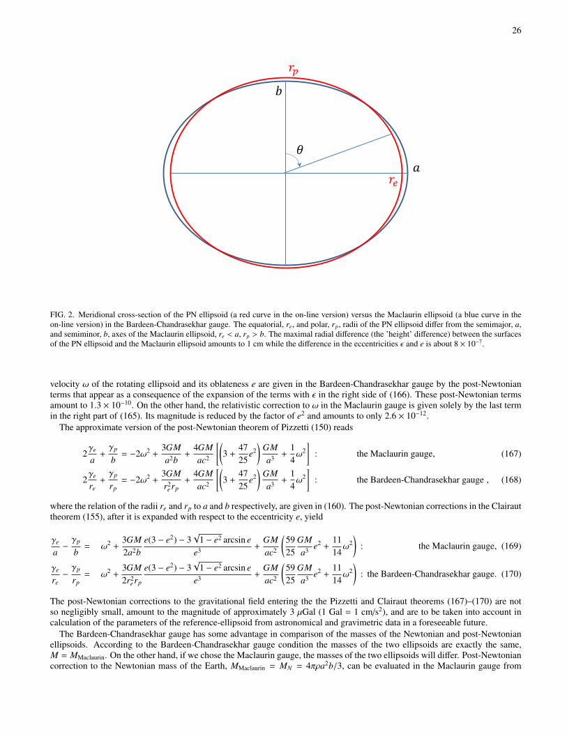
26
𝑎
𝑏
𝑟𝑒
𝑟𝑝
𝜃
FIG. 2. Meridional cross-section of the PN ellipsoid (a red curve in the on-line version) versus the Maclaurin ellipsoid (a blue curve in theon-line version) in the Bardeen-Chandrasekhar gauge. The equatorial, re, and polar, rp, radii of the PN ellipsoid differ from the semimajor, a,and semiminor, b, axes of the Maclaurin ellipsoid, re < a, rp > b. The maximal radial difference (the ’height’ difference) between the surfacesof the PN ellipsoid and the Maclaurin ellipsoid amounts to 1 cm while the difference in the eccentricities ε and e is about 8 × 10⁻⁷.
velocity ω of the rotating ellipsoid and its oblateness e are given in the Bardeen-Chandrasekhar gauge by the post-Newtonianterms that appear as a consequence of the expansion of the terms with ε in the right side of (166). These post-Newtonian termsamount to 1.3 × 10⁻¹⁰. On the other hand, the relativistic correction to ω in the Maclaurin gauge is given solely by the last termin the right part of (165). Its magnitude is reduced by the factor of e2 and amounts to only 2.6 × 10⁻¹².
The approximate version of the post-Newtonian theorem of Pizzetti (150) reads
2γe
a+γp
b= −2ω2 +
3GMa2b
+4GMac2
[(3 +
4725
e2)
GMa3 +
14ω2
]: the Maclaurin gauge, (167)
2γe
re+γp
rp= −2ω2 +
3GMr2
e rp+
4GMac2
[(3 +
4725
e2)
GMa3 +
14ω2
]: the Bardeen-Chandrasekhar gauge , (168)
where the relation of the radii re and rp to a and b respectively, are given in (160). The post-Newtonian corrections in the Clairauttheorem (155), after it is expanded with respect to the eccentricity e, yield
γe
a−γp
b= ω2 +
3GM2a2b
e(3 − e2) − 3√
1 − e2 arcsin ee3 +
GMac2
(5925
GMa3 e2 +
1114ω2
): the Maclaurin gauge, (169)
γe
re−γp
rp= ω2 +
3GM2r2
e rp
e(3 − e2) − 3√
1 − e2 arcsin ee3 +
GMac2
(5925
GMa3 e2 +
1114ω2
): the Bardeen-Chandrasekhar gauge. (170)
The post-Newtonian corrections to the gravitational field entering the the Pizzetti and Clairaut theorems (167)–(170) are notso negligibly small, amount to the magnitude of approximately 3 µGal (1 Gal = 1 cm/s2), and are to be taken into account incalculation of the parameters of the reference-ellipsoid from astronomical and gravimetric data in a foreseeable future.
The Bardeen-Chandrasekhar gauge has some advantage in comparison of the masses of the Newtonian and post-Newtonianellipsoids. According to the Bardeen-Chandrasekhar gauge condition the masses of the two ellipsoids are exactly the same,M = MMaclaurin. On the other hand, if we chose the Maclaurin gauge, the masses of the two ellipsoids will differ. Post-Newtoniancorrection to the Newtonian mass of the Earth, MMaclaurin = MN = 4πρa2b/3, can be evaluated in the Maclaurin gauge from

27
(100) which is given in the approximation under consideration, by
M = MN
[1 + 2κ
(0ג +
ω2
5πGρ
)]. (171)
Because the mass couples with the universal gravitational constant G, it contributes to the numerical value of the geocentricgravitational constant GM⊕ = 3.986004418 × 10¹⁴ m3s−2 [2, Table 1.1]. After expansion of the right side of (171) with respectto the eccentricity e, the relativistic variation in the value of GM⊕ is
δ(GM⊕)pN
GM⊕' 2κ0ג ' 4κ ' 2.8 × 10⁻⁹ . (172)
The current uncertainty in the numerical value of GM⊕ is 8 × 10⁵ m3s−2 [2, Table 1.1] which gives the fractional uncertainty
δ(GM⊕)GM⊕
' 2.0 × 10⁻⁹ . (173)
This is comparable with the relativistic contribution (172) which must be taken into account in the reduction of precise geodeticdata processing if the Maclaurin gauge is adopted in the post-Newtonian geodesy.
Similar considerations tells us that in the Bardeen-Chandrasekhar gauge the Newtonian and post-Newtonian values of theangular momentum of the Earth are exactly the same, S = S Maclaurin. However, if we chose the Maclaurin gauge we shouldexpect the difference between the Newtonian and relativistic angular momenta given by (114) which, in the approximationwhere all terms of the order of O
(e4
)are discarded, reads
S = S N
[1 +
27κ
(0ג12 − 1ג16 +
3ω2
5πGρ
)]. (174)
The fractional difference between the relativistic and Newtonian angular momenta of the Earth is
δSS'
4071ג ' 2 × 10⁻⁹ . (175)
It should be noted however that the difference (175) is not so important in geodesy because the angular momentum of the earth isnot yet directly measurable quantity as contrasted with the angular velocity ω which is measured directly by Very Long BaselineInterferometry (VLBI) of the IERS.
AsknowledgementsWe thank anonymous referees for their valuable comments and suggestions for improving the presentation of the manuscript.The work of S. M. Kopeikin and E. M. Mazurova has been supported by the grant14-27-00068 of the Russian Scientific Foun-dation. The research of W.-B. Han has been funded by the National Natural Science Foundation of China (grant 11273045)and the China Scholarship Council Fellowship201304910030. E. M. Mazurova and W.-B. Han are grateful to the Departmentof Physics and Astronomy of the University of Missouri in Columbia (USA) for hospitality.
[1] J. Kovalevsky, I. I. Mueller, and B. Kolaczek. Reference frames in astronomy and geophysics. Dordrecht, Kluwer Academic Publishers,Astrophysics and Space Science Library, Vol. 154, 482 pp., 1989.
[2] G. Petit and B. Luzum. IERS Conventions (2010). IERS Technical Note, 36:179 pp., 2010.[3] S. M. Kopejkin. Relativistic manifestations of gravitational fields in gravimetry and geodesy. Manuscripta Geodaetica, 16:301–312,
January 1991.[4] J. Muller, M. Soffel, and S. A. Klioner. Geodesy and relativity. Journal of Geodesy, 82:133–145, March 2008.[5] C. M. Will. The Confrontation between General Relativity and Experiment. Living Reviews in Relativity, 17:4, June 2014.[6] S. Chandrasekhar. Ellipsoidal figures of equilibrium - a historical account. Communications on Pure and Applied Mathematics,
20(2):251–265, 1967.[7] S. Chandrasekhar. The Post-Newtonian Effects of General Relativity on the Equilibrium of Uniformly Rotating Bodies. I. The Maclaurin
Spheroids and the Virial Theorem. Astrophys. J., 142:1513–1518, November 1965.[8] J. M. Bardeen. A Reexamination of the Post-Newtonian Maclaurin Spheroids. Astrophys. J., 167:425, August 1971.[9] S. Kopeikin, M. Efroimsky, and G. Kaplan. Relativistic Celestial Mechanics of the Solar System. Wiley, Berlin, xxxii+860 pp., September
2011.[10] E. Mai. Time, atomic clocks, and relativistic geodesy. Report No 124, Deutsche Geod’atische Kommission der Bayerischen Akademie
der Wissenschaften (DGK), 2014, 128 pp. Available online: http://dgk.badw.de/fileadmin/docs/a-124.pdf , 2014.

28
[11] S. Chandrasekhar. The Post-Newtonian Effects of General Relativity on the Equilibrium of Uniformly Rotating Bodies. II. The DeformedFigures of the Maclaurin Spheroids. Astrophys. J., 147:334–352, January 1967.
[12] S. Chandrasekhar. The Post-Newtonian Effects of General Relativity on the Equilibrium of Uniformly Rotating Bodies. III. The DeformedFigures of the Jacobi Ellipsoids. Astrophys. J., 148:621–644, May 1967.
[13] S. Chandrasekhar. The Post-Newtonian Effects of General Relativity on the Equilibrium of Uniformly Rotating Bodies.IV. The RocheModel. Astrophys. J., 148:645–649, May 1967.
[14] S. Chandrasekhar. The Post-Newtonian Effects of General Relativity on the Equilibrium of Uniformly Rotating Bodies. V. The DeformedFigures of the Maclaurin Spheroids (Continued). Astrophys. J., 167:447–453, August 1971.
[15] S. Chandrasekhar. The Post-Newtonian Effects of General Relativity on the Equilibrium of Uniformaly Rotating Bodies.VI. The De-formed Figures of the Jacobi Ellipsoids (Continued). Astrophys. J., 167:455–463, August 1971.
[16] S. Chandrasekhar and J. C. Miller. On slowly rotating homogeneous masses in general relativity. Mon. Not. Roy. Astron. Soc., 167:63–80,April 1974.
[17] S. Chandrasekhar and D. D. Elbert. The deformed figures of the Dedekind ellipsoids in the post-Newtonian approximation to generalrelativity. Astrophys. J., 192:731–746, September 1974.
[18] S. Chandrasekhar and D. D. Elbert. The deformed figures of the Dedekind ellipsoids in the post-Newtonian approximation to generalrelativity - Corrections and amplifications. Astrophys. J., 220:303–313, February 1978.
[19] K. A. Pyragas, N. P. Bondarenko, and O. V. Kravtsov. On the Equilibrium Figures of an Ideal Rotating Liquid in the Post-NewtonianApproximation of General Relativity. I: Equilibrium Conditions. Astrophysics and Space Science, 27:437–452, April 1974.
[20] N. P. Bondarenko and K. A. Pyragas. On the Equilibrium Figures of an Ideal Rotating Liquid in the Post-Newtonian Approximation ofGeneral Relativity. II: Maclaurin’s P-Ellipsoid. Astrophysics and Space Science, 27:453–466, April 1974.
[21] K. A. Pyragas, N. P. Bondarenko, and A. N. Kryshtal. On the equilibrium figures of an ideal rotating fluid in the post-Newtonianapproximation of general relativity. III - Stability of the forms of equilibrium. Astrophysics and Space Science, 33:75–97, March 1975.
[22] A. N. Tsirulev and V. P. Tsvetkov. Rotating Post-Newtonian Near Ellipsoidal Configurations of a Magnetized Homogeneous Fluid - PartOne. Soviet Astronomy, 26:289–292, June 1982.
[23] A. N. Tsirulev and V. P. Tsvetkov. Rotating Post-Newtonian Near Ellipsoidal Configurations of a Magnetized Homogeneous Fluid - PartTwo. Soviet Astronomy, 26:407–412, August 1982.
[24] V. P. Tsvetkov and A. N. Tsirulev. Gravitational Waves Emitted by a Spinning Magnetized Blob of Homogeneous Post-NewtonianGravitating Fluid. Soviet Astronomy, 27:66–69, February 1983.
[25] D. V. Galtsov, V. P. Tsvetkov, and A. N. Tsirulev. The spectrum and polarization of the gravitational radiation of pulsars. Sov. Phys.JETP, 59:472–477, 1984.
[26] D. Petroff. Post-Newtonian Maclaurin spheroids to arbitrary order. Phys. Rev. D, 68(10):104029, November 2003.[27] M. Ansorg, T. Fischer, A. Kleinwachter, R. Meinel, D. Petroff, and K. Schobel. Equilibrium configurations of homogeneous fluids in
general relativity. Mon. Not. Roy. Astron. Soc., 355:682–688, December 2004.[28] R. Meinel, M. Ansorg, A. Kleinwachter, G. Neugebauer, and D. Petroff. Relativistic Figures of Equilibrium. Cambridge University Press,
Cambridge, ix+218 pp., June 2008.[29] N. Gurlebeck and D. Petroff. The Axisymmetric Case for the Post-Newtonian Dedekind Ellipsoids. Astrophys. J., 722:1207–1215,
October 2010.[30] N. Gurlebeck and D. Petroff. A Generalized Family of Post-Newtonian Dedekind Ellipsoids. Astrophys. J., 777:1–16, November 2013.[31] H.-P. Plag and M. Pearlman (Eds). Global Geodetic Observing System. Dordrecht: Springer, 322 pp., 2009.[32] H. Drewes (Ed). Geodetic Reference Frames. Berlin: Springer, 321 pp., 2009.[33] N. Poli, C. W. Oates, P. Gill, and G. M. Tino. Optical atomic clocks. Nuovo Cimento Rivista Serie, 36:555–624, December 2013.[34] P. Komar, E. M. Kessler, M. Bishof, L. Jiang, A. S. Sorensen, J. Ye, and M. D. Lukin. A quantum network of clocks. Nature Physics,
10:582–587, August 2014.[35] R. Bondarescu, M. Bondarescu, G. Hetenyi, L. Boschi, P. Jetzer, and J. Balakrishna. Geophysical applicability of atomic clocks: direct
continental geoid mapping. Geophysical Journal International, 191:78–82, October 2012.[36] R. Bondarescu, A. Scharer, A. Lundgren, G. Hetenyi, N. Houlie, P. Jetzer, and M. Bondarescu. Ground-based optical atomic clocks as a
tool to monitor vertical surface motion. Geophysical Journal International, 202:1770–1774, September 2015.[37] S. Falke, N. Lemke, C. Grebing, B. Lipphardt, S. Weyers, V. Gerginov, N. Huntemann, C. Hagemann, A. Al-Masoudi, S. Hafner, S. Vogt,
U. Sterr, and C. Lisdat. A strontium lattice clock with 3 × 10⁻¹⁷ inaccuracy and its frequency. New Journal of Physics, 16(7):073023,2014.
[38] E. Mai and J. Muller. General remarks on the potential use of atomic clocks in relativistic geodesy. ZFV - Zeitschrift fur Geodasie,Geoinformation und Landmanagement, Vol. 138 (4) , pp. 257-266, 138:257–266, April 2013.
[39] G. Petit, P. Wolf, and P. Delva. Atomic time, clocks, and clock comparisons in relativistic spacetime: a review. In: Frontiers in RelativisticCelestial Mechanics. Vol. 2 Applications and Experiments, Ed. S. Kopeikin, De Gruyter, Berlin, 2014, pp. 249-279, .
[40] T. L. Nicholson, S. L. Campbell, R. B. Hutson, G. E. Marti, B. J. Bloom, R. L. McNally, W. Zhang, M. D. Barrett, M. S. Safronova, G. F.Strouse, W. L. Tew, and J. Ye. Systematic evaluation of an atomic clock at 2 × 10⁻¹⁸ total uncertainty. Nature Communications, 6:1–8,April 2015.
[41] M. H. Soffel. Relativity in Astrometry, Celestial Mechanics and Geodesy. Springer-Verlag, Berlin, Germany, 1989, XIV+ 208 pp., 1989.[42] C. M. Will. Theory and Experiment in Gravitational Physics. Cambridge, UK: Cambridge University Press, 396 pp., March 1993.[43] W. Torge and J. Muller. Geodesy. De Gruyter, Berlin, 4-th edition, 433 pp., 2012.[44] P. Pizzetti. Principii della teoria meccanica della figura dei pianeti. E. Spoerri, Pisa, XIII+251 pp., 1913.[45] J. Zund. Foundations of differential geodesy. Berlin: Springer-Verlag, 373 pp., 1994.[46] M. Soffel, S. A. Klioner, G. Petit, P. Wolf, S. M. Kopeikin, P. Bretagnon, V. A. Brumberg, N. Capitaine, T. Damour, T. Fukushima,
B. Guinot, T.-Y. Huang, L. Lindegren, C. Ma, K. Nordtvedt, J. C. Ries, P. K. Seidelmann, D. Vokrouhlicky, C. M. Will, and C. Xu.

29
The IAU 2000 Resolutions for Astrometry, Celestial Mechanics, and Metrology in the Relativistic Framework: Explanatory Supplement.Astron. J. (USA), 126:2687–2706, December 2003.
[47] V. A. Brumberg. Essential relativistic celestial mechanics. Adam Hilger, Bristol, 271 pp., 1991.[48] A. D. Rendall. Convergent and divergent perturbation series and the post-minkowskian approximation scheme. Classical and Quantum
Gravity, 7(5):803–812, 1990.[49] V. A. Fock. The theory of space, time and gravitation. New York, Macmillan, 2d rev. ed. Translated from the Russian by N. Kemmer. 448
pp., December 1964.[50] S. Weinberg. Gravitation and Cosmology: Principles and Applications of the General Theory of Relativity. New York: John Wiley &
Sons, Inc., July 1972.[51] S. M. Kopeikin, (Ed). Frontiers in Relativistic Celestial Mechanics. Theory., volume 1. De Gruyter, Berlin, XVI+350 pp., 2014.[52] M. Afanasiev, D. Peter, K. Sager, S. Simute, L. Ermert, L. Krischer, and A. Fichtner. Foundations for a multiscale collaborative Earth
model. Geophysical Journal International, 204:39–58, January 2016.[53] S. Chandrasekhar. Ellipsoidal figures of equilibrium. New Haven: Yale University Press, IX+252 pp., 1969.[54] W. A. Heiskanen and H. Moritz. Physical geodesy. San Francisco, W. H. Freeman, 364 pp., 1967.[55] B. Hofmann-Wellenhof and H. Moritz. Physical Geodesy. Springer, Berlin, 2006.[56] S. M. Kopeikin. Reference ellipsoid and geoid in chronometric geodesy. Frontiers in Fundamental Astronomy, 1:1–15, February 2016.[57] Y. Imanishi, T. Sato, T. Higashi, W. Sun, and S. Okubo. A Network of Superconducting Gravimeters Detects Submicrogal Coseismic
Gravity Changes. Science, 306:476–478, October 2004.[58] J. Flury and R. Rummel. Future Satellite Gravimetry for Geodesy. Earth Moon and Planets, 94:13–29, April 2004.[59] H. J. Paik. Tests of general relativity in earth orbit using a superconducting gravity gradiometer. Advances in Space Research, 9:41–50,
1989.[60] S. N. Bagaev, L. B. Bezrukov, N. L. Kvashnin, V. A. Krysanov, S. I. Oreshkin, A. M. Motylev, S. M. Popov, V. N. Rudenko, A. A.
Samoilenko, M. N. Skvortsov, and I. S. Yudin. A high frequency resonance gravity gradiometer. Review of Scientific Instruments,85(6):065114, June 2014.
[61] A. Sugarbaker, A. Black, M. Ledbetter, T. Hong, M. Kasevich, B. Saif, S. Luthcke, B. Seery, L. Feinberg, J. Mather, and R. Keski-Kuha.Cold Atom Gravity Gradiometer for Geodesy. In APS Division of Atomic, Molecular and Optical Physics Meeting Abstracts, pageK1066, May 2015.
[62] Speaking more rigorously, the surface of the fourth order is to be called a spheroid. We shall show in the last section XI of this paperthat, by making use of the coordinate freedom of general relativity, the deviations of the shape of the PN-ellipsoid from the Maclaurinellipsoid can be made so small that they can be ignored in practical applications.
[63] R. M. Wald. General relativity. University of Chicago Press, Chicago, USA, 1984, 506 pp.[64] S. M. Kopeikin, E. M. Mazurova, and A. P. Karpik. Towards an exact relativistic theory of Earth’s geoid undulation. Physics Letters A,
379:1555–1562, August 2015.[65] M. Oltean, R. J. Epp, P. L. McGrath, and R. B. Mann. Geoids in General Relativity: Geoid Quasilocal Frames. ArXiv e-prints, October
2015.[66] Strictly speaking, Bardeen [8] proposed to equate the post-Newtonian mass of baryons making up the Maclaurin and post-Newtonian
ellipsoids. The difference between the Newtonian mass of baryons and its post-Newtonian counterpart is constant [42], and is included tothe post-Newtonian mass MpN in our calculations.
[67] W. Torge. Gravimetry. Berlin, W. de Gruyter, 482 pp., 1989.[68] Because the PN ellipsoid is axisymmetric it does not matter which point on equator is taken for calculating the force of gravity. Tradi-
tionally, the force of gravity is taken at the point lying on y axis [43, 54] by convention.[69] Theorem of Stokes-Poincare states [43, section 4.2.1] that if a body of total mass M rotates with constant angular velocity ω about a
fixed axis, and if S is a level surface of its gravity field enclosing the entire mass, then the gravity potential in the exterior space of S isuniquley determined by M, ω, and the parameters defining S. In case of the level ellipsoid with the surface S such parameters are a, b.
[70] M. Soffel and R. Langhans. Space-Time Reference Systems. Springer, Berlin, XIV+314 pp., 2013.[71] S. M. Kopeikin, (Ed). Frontiers in Relativistic Celestial Mechanics. Applications and Experiments., volume 2. De Gruyter, Berlin,
XXIX+288 pp., 2014.
Appendix A: Integrals
Integrals entering equations (48), (49), (61), (62), (77), (78) are solved in two steps:
1. integrating with respect to the angle λ from 0 to 2π,
2. integrating with respect to the angle θ from 0 to π by making use of a new variable
u = b2 tan2 θ , du = 2b2 sec3 θ sin θdθ , (A1)
which changes from 0 to∞.
In terms of the new variable we have
sin θ =
√u
b2 + u, cos θ =
b√
b2 + u, (A2)

30
and
A =1a2
a2 + ub2 + u
,dΩ
A=
a2b2
dλdu
(a2 + u)√
b2 + u. (A3)
We use these values for transforming integrands in (48), (49) where we also take into account that all functions entering theintegrands are even functions of the argument, f (cos θ) = f (− cos θ). Thus, it makes∫ π
0f (cos θ) sin θdθ = 2
∫ π/2
0f (cos θ) sin θdθ . (A4)
. This procedure allows us to represent the integrals under discussion in the following form:
J0 ≡
∮S 2
dΩ
A= 2πa2b
∞∫0
du
(a2 + u)√
b2 + u, (A5a)
J1 ≡
∮S 2
cos2 θ
A2 dΩ = 2πa4b3
∞∫0
du
(a2 + u)2√
b2 + u, (A5b)
J2 ≡
∮S 2
BA2 cos θdΩ = 2πa4bz
∞∫0
du
(a2 + u)2√
b2 + u, (A5c)
J3 ≡
∮S 2
BA3 cos3 θdΩ = 2πa6b3z
∞∫0
du
(a2 + u)3√
b2 + u, (A5d)
J4 ≡
∮S 2
cos4 θ
A3 dΩ = 2πa6b5
∞∫0
du
(a2 + u)3√
b2 + u, (A5e)
J5 ≡
∮S 2
B2
A2 dΩ =πa2
b
∞∫
0
b2u + (2a2 − u)z2
(a2 + u)2√
b2 + udu + b2C(x)
∞∫0
udu
(a2 + u)2√
b2 + u
, (A5f)
J6 ≡
∮S 2
B2
A4 cos4 θdΩ = πa6b3
∞∫
0
b2u + (2a2 − u)z2
(a2 + u)4√
b2 + udu + b2C(x)
∞∫0
udu
(a2 + u)4√
b2 + u
, (A5g)
J7 ≡
∮S 2
B2
A3 cos2 θdΩ = πa4b
∞∫
0
b2u + (2a2 − u)z2
(a2 + u)3√
b2 + udu + b2C(x)
∞∫0
udu
(a2 + u)3√
b2 + u
, (A5h)
J8 ≡
∮S 2
B3
A4 cos3 θdΩ = πa6bz
∞∫
0
3b2u + (2a2 − 3u)z2
(a2 + u)4√
b2 + udu + 3b2C(x)
∞∫0
udu
(a2 + u)4√
b2 + u
, (A5i)
J9 ≡
∮S 2
B4
A5 cos4 θdΩ =πa6b
4
∞∫0
3b4u2 + 6b2u(4a2 − u)z2 + (8a4 − 24a2u + 3u2)z4
(a2 + u)5√
b2 + udu (A5j)
+32
C(x)πa6b3
∞∫
0
(b2 − z2
)u2 + 4a2uz2
(a2 + u)5√
b2 + udu +
b2
2C(x)
∞∫0
u2du
(a2 + u)5√
b2 + u
,J10 ≡
∮S 2
B3
A3 sin θ cos λdΩ =3πa2x
4b
∞∫
0
(b2u + 4a2z2 − uz2
)udu(
a2 + u)3 √b2 + u
+ b2C(x)
∞∫0
u2du(a2 + u
)3 √b2 + u
, (A5k)
J11 ≡
∮S 2
B3
A3 sin θ sin λdΩ =3πa2y
4b
∞∫
0
(b2u + 4a2z2 − uz2
)udu(
a2 + u)3 √b2 + u
+ b2C(x)
∞∫0
u2du(a2 + u
)3 √b2 + u
, (A5l)
J12 ≡
∮S 2
B3
A3 cos θdΩ =πa4z
b
∞∫
0
(3b2u + 2a2z2 − 3uz2
)du(
a2 + u)3 √b2 + u
+ 3b2C(x)
∞∫0
udu(a2 + u
)3 √b2 + u
, (A5m)
31
J13 ≡
∮S 2
BA2 sin θ cos λdΩ = πa2bx
∞∫0
udu(a2 + u
)2 √b2 + u, (A5n)
J14 ≡
∮S 2
BA2 sin θ sin λdΩ = πa2by
∞∫0
udu(a2 + u
)2 √b2 + u, (A5o)
J15 ≡
∮S 2
B4
A3 dΩ =πa2
4b3
∞∫0
3b4u2 + 6b2u(4a2 − u)z2 + (8a4 − 24a2u + 3u2)z4
(a2 + u)3√
b2 + udu (A5p)
+32
C(x)πa2
b
∞∫
0
(b2 − z2
)u2 + 4a2uz2
(a2 + u)3√
b2 + udu +
b2
2C(x)
∞∫0
u2du
(a2 + u)3√
b2 + u
,J16 ≡
∮S 2
B4
A4 cos2 θdΩ =πa4
4b
∞∫0
3b4u2 + 6b2u(4a2 − u)z2 + (8a4 − 24a2u + 3u2)z4
(a2 + u)4√
b2 + udu (A5q)
+32
C(x)πa4b
∞∫
0
(b2 − z2
)u2 + 4a2uz2
(a2 + u)4√
b2 + udu +
b2
2C(x)
∞∫0
u2du
(a2 + u)4√
b2 + u
,These integrals can be performed analytically,
J0 ≡ 2πa20ג , (A6a)J1 ≡ 2πa2b21ג , (A6b)J2 = 2πa2z1ג , (A6c)J3 ≡ 2πa2b2z2ג , (A6d)J4 ≡ 2πa2b42ג , (A6e)
J5 = πa2[(
1 −z2
b2
)0ג −
(1 − 3
z2
b2
)1ג + C(x) 0ג) − (1ג
], (A6f)
J6 ≡ πa2b4[(
1 −z2
b2
)2ג −
(1 −
3z2
b2
)3ג + C(x) 2ג) − (3ג
], (A6g)
J7 = πa2b2[(
1 −z2
b2
)1ג −
(1 − 3
z2
b2
)2ג + C(x) 1ג) − (2ג
], (A6h)
J8 = 3πa2b2z[(
1 −z2
b2
)2ג −
(1 −
53
z2
b2
)3ג + C(x) 2ג) − (3ג
], (A6i)
J9 =34πa2b4
(1 − z2
b2
)2
2ג − 2(1 − 6
z2
b2 + 5z4
b4
)3ג +
(1 − 10
z2
b2 +353
z4
b4
)4ג
(A6j)
+32
C(x)πa2b4[(
1 −z2
b2
)2ג − 2
(1 −
3z2
b2
)3ג +
(1 −
5z2
b2
)4ג
]+
34
C2(x)πa2b4 2ג) − 3ג2 + (4ג ,
J10 =34πa2x
[(1 −
z2
b2
)0ג − 2
(1 −
3z2
b2
)1ג +
(1 −
5z2
b2
)2ג + C(x) 0ג) − 1ג2 + (2ג
], (A6k)
J11 =34πa2y
[(1 −
z2
b2
)0ג − 2
(1 −
3z2
b2
)1ג +
(1 −
5z2
b2
)2ג + +C(x) 0ג) − 1ג2 + (2ג
], (A6l)
J12 = 3πa2x[(
1 −z2
b2
)1ג −
(1 −
53
z2
b2
)2ג + C(x) 1ג) − (2ג
], (A6m)
J13 = πa2x 0ג) − (1ג , (A6n)J14 = πa2y 0ג) − (1ג , (A6o)
J15 =34πa2
(1 − z2
b2
)2
0ג − 2(1 − 6
z2
b2 + 5z4
b4
)1ג +
(1 − 10
z2
b2 +353
z4
b4
)2ג
(A6p)

32
+32
C(x)πa2[(
1 −z2
b2
)0ג − 2
(1 −
3z2
b2
)1ג +
(1 −
5z2
b2
)2ג
]+
34
C2(x)πa2 0ג) − 1ג2 + (2ג ,
J16 =34πa2b2
(1 − z2
b2
)2
1ג − 2(1 − 6
z2
b2 + 5z4
b4
)2ג +
(1 − 10
z2
b2 +353
z4
b4
)3ג
(A6q)
+32
C(x)πa2b2[(
1 −z2
b2
)1ג − 2
(1 −
3z2
b2
)2ג +
(1 −
5z2
b2
)3ג
]+
34
C2(x)πa2 1ג) − 2ג2 + (3ג ,
where
nג ≡ a2nb
∞∫0
du
(a2 + u)n+1√
b2 + u=
2√
1 − e2
e2(n+1)
∞∫√
1−e2e
dξ(1 + ξ2)n+1 . (A7)
is a table integral given in (Gradshteyn and Ryzhik, integral 2.148-4)
nג =(2n − 1)!!
2n−1n!
√1 − e2
e2n+1 arcsin e −(1 − e2
) n∑k=1
(n − k)!(2n − 2k + 1)!!
2n−k
e2k
. (A8)
In particular,
0ג = 2
√1 − e2
earcsin e , (A9a)
1ג =
√1 − e2
e3 arcsin e −1 − e2
e2 , (A9b)
2ג =34
√1 − e2
e5 arcsin e −(1 − e2)(3 + 2e2)
4e4 , (A9c)
3ג =58
√1 − e2
e7 arcsin e −(1 − e2)(15 + 10e2 + 8e4)
24e6 , (A9d)
4ג =3564
√1 − e2
e9 arcsin e −(1 − e2)(105 + 70e2 + 56e4 + 48e6)
192e8 (A9e)
There is also a recurrent formula that allows us to calculate the integrals nג by iterations starting from ,0ג
nג =2n − 1
2nn−1ג
e2 −1 − e2
ne2 (n ≥ 1) . (A10)
where 0ג is given in (A9a). Notice that none of these integrals is divergent for small values of the eccentricity because thedenominators of the integrals suppress the small value of the eccentricity in the numerator.