i+ i - ceaa-acee.gc.ca · pdf filecolumbia to markets in china and california with tankers of...

I+ I Department of Justice Canada

Prairie Region 301-310 Broadway Winnipeg, Manitoba R3C 056

November 16,2012

Ministere de Ia Justice Canada

Region des prairies 310, Broadway piece 301 Winnipeg (Manitoba) R3COS6

VIA ELECTRONIC FILING TO FOLLOW BY COURIER

Secretary to the Joint Review Panel Enbridge Northern Gateway Project 444- Seventh AvenueS. W. Calgary, Alberta T2P OX8

Attention: Ms. Sheri Young

Dear Madam:

Re: Hearing Order OH-4-2011 Enbridge Northern Gateway Project

S=rity Classification :

Telephone:

Facsimile: Internet:

Our File: Notre dossier:

Fisheries and Oceans Canada - Further Written Evidence

(204) 984-6961 (204) 984-6488

[email protected]

2-128959

Further to JRP Rulings 105 and 120, attached hereto for filing please find Fisheries and Oceans Canada's written evidence describing potential tsunamis associated with two historical submarine slope failures discovered in 2012 in Douglas Channel by Natural Resources Canada:

1. Modelling Tsunamis Associated with Recently Identified Slope Failures in Douglas Channel; and

2. Numerical simulation of tsunamis generated by submarine slope failures in Douglas Channel, British Columbia.

This information, which includes wave heights, current speeds, wave periods, and wave propagation times, ensures that the Joint Review Panel has the most up to date information.

Canada

(A49231)

- 2-

Should you have any questions or require anything further, kindly contact the undersigned.

Yours truly,

Dayna S. Anderson Counsel Prairie Region Department of Justice Canada

cc: Parties to OH-4-2011

(A49231)

Pacific Region Canadian Science Advisory Secretariat

Science Response 2012/037

October 2012

MODELLING TSUNAMIS ASSOCIATED WITH RECENTLY IDENTIFIED SLOPE FAILURES IN DOUGLAS CHANNEL

Context Enbridge Northern Gateway Pipelines Ltd. has proposed to construct and operate the infrastructure for the conveyance and export of diluted bitumen from Alberta to overseas markets and import of petroleum condensates for use in oil sands production.

Fisheries and Oceans Canada (DFO) is participating in an environmental assessment by a Joint Review Panel environmental assessment. A Joint Review Panel is an independent body, mandated by the Minister of the Environment and the National Energy Board. The Panel will assess the environmental effects of the proposed project and review the application under both the Canadian Environmental Assessment Act and the National Energy Board Act.

On August 17, 2012, a Notice of Motion of the Attorney General of Canada Seeking to Tender Supplementary Written Evidence was filed and subsequently granted with the Joint Review Panel “Respecting Two Previously Unrecognized Submarine Slope Failures in the Douglas Channel and A Future Additional Assessment of the Tsunami Potential Associate with these Two Slope Failures”. DFO Science, Pacific Region was requested to provide an additional assessment consisting of modeling of the wave heights and speeds that may have resulted from two previously unrecognized submarine slope failures in the Douglas Channel. This analysis will be provided to the Panel and parties before the Panel to ensure they have the most up to date information of geo-hazards in Douglas Chanel. Due to the urgency of the request a Canadian Science Advisory Secretariat (CSAS) Science Special Response Process (SSRP) was utilized to provide this information.

Specifically, the objective of this assessment is to provide an analysis of numerically simulated tsunami wave heights, current speeds, wave periods, and wave propagation times that would have been generated from a slide of material from the recently identified submarine slope failures in Douglas Channel.

This Science Response report is from the Fisheries and Oceans Canada, Canadian Science Advisory Secretariat, Regional Science Special Response Process (SSRP) of October 29th, 2012. All material contained herein is based on the technical publication Thomson et al. 2012. Numerical simulation of tsunamis generated by submarine slope failures in Douglas Channel, British Columbia. DFO Can. Sci. Advis. Sec. Res. Doc. 2012/155.

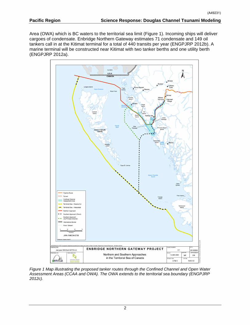
Background The Enbridge Northern Gateway Project proposes to ship dilute bitumen from Kitimat, British Columbia to markets in China and California with tankers of the class Very Large Crude Carriers (VLCC) (Enbridge Northern Gateway Project Joint Review Panel (ENGPJRP) 2012a). The tanker route from Kitimat through confined waterways in British Columbia and then into open waters of Hecate Strait, Dixon Entrance and Queen Charlotte Sound in British Columbia are illustrated in Figure 1. For assessment purposes Enbridge Northern Gateway defines two areas, the Confined Channel Assessment Area (CCAA) (Figure 2) and the Open Water Assessment

(A49231)

Pacific Region Science Response: Douglas Channel Tsunami Modeling

Area (OWA) which is BC waters to the territorial sea limit (Figure 1). Incoming ships will deliver cargoes of condensate. Enbridge Northern Gateway estimates 71 condensate and 149 oil tankers call in at the Kitimat terminal for a total of 440 transits per year (ENGPJRP 2012b). A marine terminal will be constructed near Kitimat with two tanker berths and one utility berth (ENGPJRP 2012a).

Figure 1 Map illustrating the proposed tanker routes through the Confined Channel and Open Water Assessment Areas (CCAA and OWA). The OWA extends to the territorial sea boundary (ENGPJRP 2012c).

2

(A49231)


Slide A

Slide B

Figure 2 Map illustrating the location and extent of the Confined Channel Assessment Area (CCAA) (ENGPJRP 2012c)

3

(A49231)


Rationale for Assessment On August 17, 2012, a Notice of Motion of the Attorney General of Canada Seeking to Tender Supplementary Written Evidence was filed with the Joint Review Panel “Respecting Two Previously Unrecognized Submarine Slope Failures in the Douglas Channel and A Future Additional Assessment of the Tsunami Potential Associate with these Two Slope Failures”.

Multibeam bathymetric surveys by the Canadian Hydrographic Service and Natural Resources Canada revealed the presence of two large submarine landslides along the southeastern side of Douglas Channel in northwestern British Columbia. The landslides likely date from sometime in the early to mid-Holocene (10,000 to 5,000 years ago). These failures could have forced landslide-generated tsunamis, and conditions exist for similar failures and associated tsunamis to occur along this segment of Douglas Channel in the future (Conway et al, 2012).

DFO Science, Pacific Region was requested to provide an additional assessment consisting of modeling of the wave heights and speeds that may have resulted from two previously unrecognized submarine slope failures in the Douglas Channel. This analysis will be provided to the Panel and parties before the Panel to ensure they have the most up to date information on geohazards in Douglas Chanel.

Analysis and Responses

Slide Reconstructions Coastal British Columbia is an area of steep slopes, extreme seasonal variations in soil moisture, large tidal ranges, and the highest seismicity in Canada. Hazards of this form have been well documented for the coastal region of British Columbia, and other fjord regions of the world’s oceans, including Alaska and Norway. These factors increase the potential for both submarine and subaerial slope failures in the region. Such events generally take place in relatively shallow and confined inner coastal waterways, and can present hazards in terms of tsunami wave generation.

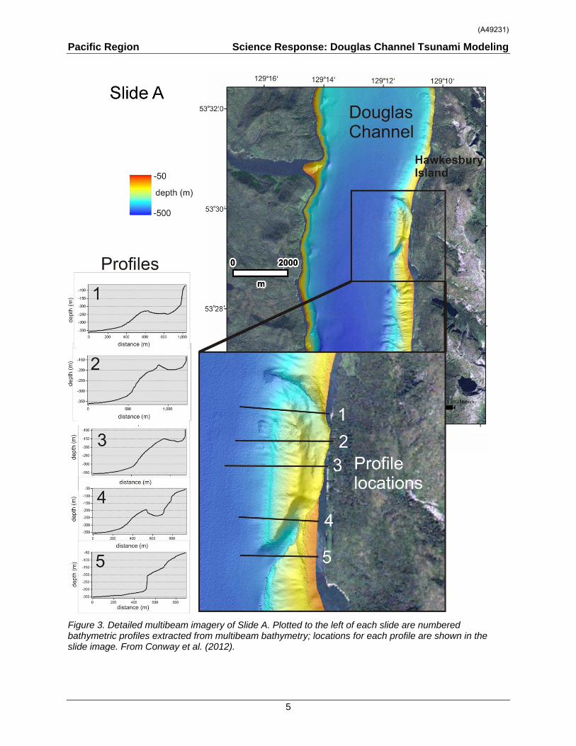
The two submarine slide regions recently identified are located 10 km apart on the eastern slope of southern Douglas Channel, near the southern end of Hawkesbury Island (Figures 3 and 4 (Conway et al. 2012)). The failures are defined by scallop-shaped hollows located along the edge of the fiord wall and appear to be associated with detached blocks that extend out several hundred metres into the channel. The two block slides identified in Douglas Channel are characteristic of rigid-body submarine landslides, which differ considerably from the well-documented viscous submarine landslides with a lower specific gravity (density relative to water) of about 1.5 that occurred to the north of Douglas Channel along the inner slope of Kitimat Arm in 1974 and 1975.

Conway et al. (2012) estimate the volumes of the two slides to have been 32 million m3 for Slide A and 31 million m3 for Slide B (Figure 3 and 4 respectively).

4

(A49231)


Figure 3. Detailed multibeam imagery of Slide A. Plotted to the left of each slide are numbered bathymetric profiles extracted from multibeam bathymetry; locations for each profile are shown in the slide image. From Conway et al. (2012).

5

(A49231)


Figure 4 Detailed multibeam imagery of Slide B. Plotted to the left of each slide are numbered bathymetric profiles extracted from multibeam bathymetry; locations for each profile are shown in the slide image. From Conway et al. (2012).

6

(A49231)


7

However, these are considered minimum values, as they do not include debris that would have spread into the fiord after initial detachment and block sliding, which is now buried by a thick layer of post-slide sediment. The blocks are thought to be derived directly from the Hawkesbury Island coastal lithology which, according to mapping by Roddick (1970), consists of a diorite (igneous) rock with a specific gravity (density relative to water) of around 2.6.

Although there are insufficient bathymetric data to delineate the exact boundaries of the original failures, a reconstruction of the slide regions immediately prior to failure indicates the slides were wedge-shaped. The head of the more northern slide (Slide A) began at a depth of around 60 to 100 m, while that of the more southern slide (Slide B) began at a depth of 75 to 120 m. Depending on the friction between the slide and the underlying seafloor, the slides would have moved downslope with a peak velocity of approximately 25 m/s before coming to rest after a duration of about 30 seconds. Based on the multibeam data, the slides moved a distance of roughly 250 to 350 m before stopping at the base of the slope in water depths of around 400 m.

Delineations of the slide bodies are based on several assumptions which could be potential sources of error. First, the estimate of the slide thickness is determined by the depth of upper troughs observed in the multibeam data. Sediment accumulation in the region may have occurred at different rates over the slide areas, with troughs possibly filling in faster than crests and slopes. In addition, the downslope (cross-shore) extent of the slides was equated to the observed cross-shore extent of the sloped portion of the seafloor, leading to uncertainty in the estimates of slide dimensions.

Tsunami Modeling Results A numerical mathematical model was used to simulate the tsunami waves and currents that would be generated in Douglas Channel and adjoining waterways (including Kitimat Arm) by block-like submarine landslides having the dimensions of Slides A and B identified by the recent multibeam bathymetric surveys (Conway et al. 2012). The numerical simulations provide estimates of the tsunami wave amplitudes1, propagation times, wave periods, and current velocities as functions of time and location within a broad area of the inner coastal waterway.

Slide A

Slide A would have generated extremely large waves in the immediate vicinity of the failure region within a minute of the submarine landslide. Waves in the numerical simulations reach amplitudes of 30 to 40 m at the coast near the slide area (Figure 5).

1 Amplitude is ½ wave height.

(A49231)


Figure 5 Maximum tsunami wave amplitudes generated by Slide A. Expanded regions are presented in (b) and (c); see (a) for locations. Note change in amplitude units in (b). From Thomson et al. (2012).

A delay between the arrival of the first (or leading) waves and the arrival of the highest (or maximum) waves at a particular point is typical for tsunamis generated by submarine landslides in coastal regions. The delay increases with distance from the slide, because the waves undergo numerous reflections and non-linear interaction en route. Numerical results reveal maximum wave amplitudes of 6 m at Hartley Bay. Large amplitude waves with typical periods of around 50 seconds would continue for several tens of minutes.

8

(A49231)


For regions outside Douglas Channel, the simulated tsunami waves are relatively small, with typical wave amplitudes less than 1 m. The leading tsunami waves generated by Slide A reach Kitimat Arm in roughly 20 min and have small amplitudes of only a few centimetres. Although later waves have higher amplitudes, the maximum wave amplitudes (which occur 50-55 min after the failure event) are still only around 0.09 to 0.12 m.

High tsunami waves are accompanied by strong wave-induced currents. Regions with maximum wave amplitudes are associated with intense currents of up to 15 m/s. According to the model results, especially strong currents occur near the shore and at headlands close to the slide. Tsunami-induced currents are weak throughout Kitimat Arm, with typical speeds of less than 0.01-0.02 m/s. Even at headlands, the speeds of the wave-induced currents do not exceed 0.1 m/s.

Slide B

Analysis for Slide B follows the same procedure as for Slide A. An examination of the bathymetric data shows that Slide B moved roughly 400 m before stopping. Because Slide B began its movement at greater depth than Slide A, the centre of mass of Slide B underwent a smaller vertical displacement than Slide A. This, in turn, caused Slide B to move significantly slower than Slide A, leading to differences in the simulated tsunami waves generated by the two slides.

Slide B would have generated large waves in the vicinity of the failure region. Simulated waves reach the coast adjacent to the slide region within a minute of the failure event, with wave amplitudes of up to 10 m (Figure 6). The waves also hit the opposite site of the channel within a minute of the failure event and then take an additional minute to reach Hartley Bay (Figure 2), where waves reach amplitudes of 15 m. Powerful oscillations in the bay last for tens of minutes. Waves with high amplitudes (more than 2 m) also occur in the southern part of Douglas Channel, and in certain locations of Verney Passage (Figure 2)

9

(A49231)


Figure 6 Maximum tsunami wave amplitudes generated by Slide B. Expanded regions are presented in (b) and (c); see (a) for locations. Note change in amplitude units in (b). From Thomson et al. (2012).

In Verney Passage, and in other areas away from the confines of southern Douglas Channel, the tsunami waves are much smaller, with typical amplitudes of less than 0.5 m. The leading tsunami waves reach Kitimat Arm 22 minutes after the start of the slide, while maximum waves with amplitudes of 0.08 m to 0.3 m, reach Kitimat Arm 45 to 60 minutes after the start of the failure event. We note that the tsunami waves generated by Slide B that impact Kitimat Arm, although still of low amplitude, are somewhat higher than those generated by Slide A, despite the fact that Slide B is located further to the south and generates less energetic waves in the source region than Slide A. This seeming paradox is explained by the slower motion of Slide B,

10

(A49231)


which causes it to generate more wave energy in the low frequency band than Slide A. Due to their reduced scattering and reflection, the relatively long and lower frequency waves generated by Slide B propagate more readily through the complex fjord system than the relatively short and higher frequency waves generated by Slide A.

Tsunami waves generated by Slide B in the failure region are accompanied by intense currents, with maximum velocities centred in the source area. Because Slide B generated less energetic tsunami waves than Slide A, current speeds in the source area are generally less than those generated by Slide A. In Hartley Bay, currents reach 3 m/s and exceed 4 m/s in the narrow channel to the south of the bay. Near the slide zone, current speeds reach 2 m/s. In the source region, and at selected capes, the currents can be as strong as 6 m/s.

For sites outside the Douglas Channel and in adjoining channels, the tsunami-induced currents are quite weak. Although currents generated in Kitimat Arm by Slide B are slightly stronger than for Slide A, the currents are still weaker than 0.1 m/s.

Conclusions The numerical simulations show that the two identified submarine landslides would have generated tsunami waves with peak amplitudes of 30 to 40 m (wave heights of 60 to 80m), current speeds of up to 15 m/s (roughly 30 knots), wavelengths of the order of 1 km, and periods of tens of seconds to several minutes. Highest waves and strongest currents would have occured along the shoreline opposite and adjacent to the failure regions.

Because of their relatively short wavelengths, the tsunami waves undergo multiple reflections and a high degree of scattering from the complex shoreline and bottom topography in Douglas Channel. These effects, combined with the flux of tsunami energy through adjoining waterways and channels, causes rapid attenuation of the waves with distance south and north of the source region. At the estimated propagation speeds of ~65 m/s, it takes roughly 10 to 15 minutes for the simulated waves to propagate approximately 40 to 45 km to the intersection of Douglas Channel and Kitimat Arm, where peak wave amplitudes would be diminished to less than 1 m. It would have then taken another 15 minutes for the waves to reach northern Kitimat Arm, where wave amplitudes would be reduced to a few tens of centimetres and associated currents to speeds of less than a few centimetres per second.

As with the tsunami generation regions, the highest waves and strongest currents in any particular region of the coastal waterway would occur near the shoreline. Based on the numerical findings, Douglas Channel would have experienced large waves and strong currents, while Kitimat Arm would have experienced negligible waves and currents. Additional modeling would be required to assess the characteristics of possible tsunamis originating beyond the area of the two identified slope failures.

11

(A49231)


Contributors

Name Affiliation

Vaughn Barrie Natural Resources Canada, Pacific Region

Bill Crawford DFO Science, Pacific Region

Josef Cherniawsky DFO Science, Pacific Region

Kim Conway Natural Resources Canada, Pacific Region

Isaac Fine DFO Science, Pacific Region

Dave Jackson DFO Science, Pacific Region

Helen Joseph DFO Science, National Capital Region

Maxim Krassovski DFO Science, Pacific Region

Andrew Ross DFO Science, Pacific Region

Richard Thompson DFO Science, Pacific Region

Peter Wills DFO Science, Pacific Region

Marilyn Joyce (Editor) DFO Science, Pacific Region

Approved by Laura Richards

Regional Director, Science DFO Science, Pacific Region

Sidney, British Columbia

References Conway, K.W., Barrie, J.V., Thomson, R.E. 2012. Submarine slope failures and tsunami hazard

in coastal British Columbia: Douglas Channel and Kitimat Arm. Geological Survey of Canada, Current Research 2012-10, 13 p., doi:10.4095/291732.

ENGPJRP. 2012a. https://www.neb-one.gc.ca/ll-eng/livelink.exe/fetch/2000/90464/90552/384192/620327/customview.html?func=ll&objId=620327&objAction=browse&sort=-name. Accessed October 30, 2012 - Vol. 1, B1-2, Enbridge Northern Gateway Project Section 52 Application

ENGPJRP 2012b. https://www.neb-one.gc.ca/ll-eng/livelink.exe/fetch/2000/90464/90552/384192/620327/customview.html?func=ll&objId=620327&objAction=browse&sort=-name. Accessed October 30, 2012 - Vol. 8C, B3-37, Enbridge Northern Gateway Project Section 52 Application

ENGPJRP 2012c. https://www.neb-one.gc.ca/ll-eng/livelink.exe/fetch/2000/90464/90552/384192/620327/customview.html?func=ll&objId=620327&objAction=browse&sort=-name. Accessed October 30, 2012 - Volume B9-42 Enbridge Northern Gateway Project

Roddick, J.A. (compiler)1970. Douglas Channel and Hecate Strait; Geological Survey of Canada, Map 23-970 (Paper 70-41), 1:250,000

Thomson, R., Fine, I., Krassovski, M., Cherniawsky, J., Conway, K. and Wills, P. 2012. Numerical simulation of tsunamis generated by submarine slope failures in Douglas Channel, British Columbia. DFO Can. Sci. Advis. Sec. Res. Doc. 2012/155.

12

(A49231)

https://www.neb-one.gc.ca/ll-eng/livelink.exe/fetch/2000/90464/90552/384192/620327/customview.html?func=ll&objId=620327&objAction=browse&sort=-name










This Report is Available from the Centre for Science Advice - Pacific Region

Fisheries and Oceans Canada 3190 Hammond Bay Road Nanaimo, British Columbia

V9T 6N7

Telephone: 250-756-7208 E-Mail: [email protected]

Internet address: www.dfo-mpo.gc.ca/csas-sccs

ISSN 1919-3750 (Print) ISSN 1919-3769 (Online)

© Her Majesty the Queen in Right of Canada, 2012

La version française est disponible à l’adresse ci-dessus.

Correct Citation for this Publication: DFO. 2012. Modelling Tsunamis associated with recently identified slope failures in Douglas

channel. DFO Can. Sci. Advis. Sec. Sci. Resp. 2012/037.

13

(A49231)

http://www.dfo-mpo.gc.ca/csas-sccs

C S A S

Canadian Science Advisory Secretariat

S C C S

Secrétariat canadien de consultation scientifique

This series documents the scientific basis for the evaluation of aquatic resources and ecosystems in Canada. As such, it addresses the issues of the day in the time frames required and the documents it contains are not intended as definitive statements on the subjects addressed but rather as progress reports on ongoing investigations.

La présente série documente les fondements scientifiques des évaluations des ressources et des écosystèmes aquatiques du Canada. Elle traite des problèmes courants selon les échéanciers dictés. Les documents qu’elle contient ne doivent pas être considérés comme des énoncés définitifs sur les sujets traités, mais plutôt comme des rapports d’étape sur les études en cours.

Research documents are produced in the official language in which they are provided to the Secretariat. This document is available on the Internet at:

Les documents de recherche sont publiés dans la langue officielle utilisée dans le manuscrit envoyé au Secrétariat. Ce document est disponible sur l’Internet à:

http://www.dfo-mpo.gc.ca/csas-sccs

ISSN 1499-3848 (Printed / Imprimé) ISSN 1919-5044 (Online / En ligne)

© Her Majesty the Queen in Right of Canada, 2012 © Sa Majesté la Reine du Chef du Canada, 2012

Research Document 2012/155

Document de recherche 2012/155

Pacific Region Région du Pacifique Numerical simulation of tsunamis generated by submarine slope failures in Douglas Channel, British Columbia

Simulations numériques de tsunamis générés par des glissements de talus sous-marins dans le chenal Douglas, Colombie-Britannique

Richard Thomson1, Isaac Fine1, Maxim Krassovski1, Josef Cherniawsky1, Kim Conway2 and Peter Wills3

1Institute of Ocean Sciences, Fisheries and Oceans Canada 2Geological Survey of Canada-Pacific, Natural Resources Canada

3Canadian Hydrographic Service, Fisheries and Oceans Canada 9860 West Saanich Road, Sidney, BC, V8L 4B2

(A49231)

i

TABLE OF CONTENTS

TABLE OF CONTENTS ............................................................................................................... I LIST OF TABLES ........................................................................................................................ II LIST OF FIGURES ..................................................................................................................... II ABSTRACT ................................................................................................................................ III RÉSUMÉ .................................................................................................................................. IV 1. INTRODUCTION .................................................................................................................... 1 2. RECONSTRUCTION OF THE INITIAL SUBMARINE FAILURE ZONES ................................ 2

2.1 MULTIBEAM DATA FOR SLIDES A AND B ..................................................................... 2 2.2 RECONSTRUCTION OF SLIDES A AND B ..................................................................... 3 2.3 LIMITATIONS AND SOURCES OF ERROR ..................................................................... 4

3. THE NUMERICAL MODEL ..................................................................................................... 4 3.1 THE NUMERICAL DOMAIN ............................................................................................. 5 3.2 MODEL BOUNDARY CONDITIONS ................................................................................. 6 3.3 SENSITIVITY OF THE MODEL TO BATHYMETRIC SMOOTHING ................................. 6 3.4 SENSITIVITY OF THE MODEL TO CHANNEL TRUNCATION EFFECTS ....................... 7 3.5 SENSITIVITY OF THE MODEL TO 20% ERRORS IN SLIDE VOLUME ........................... 7 3.6 SENSITIVITY OF THE MODEL TO CHANGES IN SLIDE FRICTION ............................... 7

4. RESULTS ............................................................................................................................... 7 4.1 SLIDE A: STANDARD FAILURE MODEL ......................................................................... 7 4.2. SLIDE B: STANDARD FAILURE MODEL ........................................................................ 9 4.3 SENSITIVITY ANALYSES .............................................................................................. 10

4.3.1 Sensitivity to bathymetric smoothing ....................................................................... 10 4.3.2. Sensitivity to the channel truncation effects ........................................................... 11 4.3.3 Sensitivity to changes in slide volume ..................................................................... 11 4.3.3 Sensitivity to changes in slide friction ...................................................................... 12

5. DISCUSSION ........................................................................................................................ 13 6. CONCLUSIONS .................................................................................................................... 15 ACKNOWLEDGEMENTS ......................................................................................................... 16 REFERENCES ......................................................................................................................... 16 FIGURES .................................................................................................................................. 18

(A49231)

ii

LIST OF TABLES

Table 1 Slide parameters used in the numerical model. Δx is the displacement in the cross-shore direction and Δy is the corresponding displacement in the alongshore direction. ...... 4

Table 2 Slide movement parameters used in the numerical model simulations.. ........................ 8

Table 3 Principal tsunami wave statistics for specific locations in the model domain for Slide A. ..........................................................................................................................................10

Table 4 Principal tsunami wave statistics for specific locations in the model domain for Slide B. ..........................................................................................................................................10

Table 5 Sensitivity test results for maximum wave amplitude, A, and maximum speed, v.. .......13

Table 6 Tsunami wave statistics for specific locations in the model domain for Slide B. Values are derived using a reduced friction coefficient k = 0.1. .....................................................13

LIST OF FIGURES

Figure 1 The study region.. .......................................................................................................18

Figure 2 Detailed multibeam imagery of (a) Slide A and (b) Slide B.. ........................................19

Figure 3 Side view of land elevations (positive values) and water depth (negative values) in the region of submarine landslides A and B.. ..........................................................................21

Figure 4 Reconstruction of Slide A (top panels) and Slide B (bottom panels). ...........................22

Figure 5 Reconstruction of Slide A (top panels) and Slide B (bottom panels).. ..........................23

Figure 6 Reconstruction of Slide A (top panels) and Slide B (bottom panels).. ..........................24

Figure 7 Slide A. (a) Actual and (b) reconstructed final bathymetry. ..........................................25

Figure 8 As for Figure 7 but for Slide B. ....................................................................................26

Figure 9 Bathymetry (blue) and LW coastline (red) data coverage.. ..........................................27

Figure 10 Water depths for the 50-m gridded numerical model domain. ...................................28

Figure 11 Reference locations for model output.. ......................................................................29

Figure 12 Maximum tsunami wave amplitudes generated by Slide A.. ......................................30

Figure 13 Maximum current speeds generated by Slide A.. ......................................................31

Figure 14 Simulated tsunami wave amplitudes as functions of time at the reference locations (see Figure 11) for Slide A.. ...............................................................................................32

Figure 15 Tsunami zoning based on the maximum simulated tsunami wave amplitudes for Slide A. ......................................................................................................................................33

Figure 16 Maximum tsunami wave amplitudes generated by Slide B. Expanded regions are presented in (b) and (c); see (a) for locations. . .................................................................34

Figure 17 Maximum current speeds generated by Slide B.. ......................................................35

Figure 18 Simulated tsunami wave amplitudes as functions of time at the reference locations (see Figure 11) for Slide B.. ...............................................................................................36

Figure 19 Tsunami “zoning” based on the maximum simulated tsunami wave amplitudes for Slide B. ..............................................................................................................................37

Figure 20 Maximum tsunami wave amplitudes and current speeds in the source region; see area (c) in Figures 12, 13, 16, and 17. ...............................................................................38

(A49231)

iii

Correct citation for this publication:

Thomson, R., Fine, I., Krassovski, M., Cherniawsky, J., Conway, K. and Wills, P. 2012. Numerical simulation of tsunamis generated by submarine slope failures in Douglas Channel, British Columbia. DFO Can. Sci. Advis.Sec. Res. Doc. 201/155. Vi + 38p.

ABSTRACT

Multibeam bathymetric surveys by the Canadian Hydrographic Service and Natural Resources Canada have revealed the presence of two massive (~65 million cubic meter) submarine landslides along the southeastern side of Douglas Channel in northwestern British Columbia. Although the landslides likely date from the early to mid Holocene, Conway et al. (2012) suggest that these failures could have forced major landslide-generated tsunamis and that the risk of similar events in the channel in the future cannot be ruled out. We characterize this risk using a fully nonlinear, non-hydrostatic numerical mathematical model to simulate the tsunami waves that would have been generated by the two slides were they to occur during present-day marine conditions in southern Douglas Channel. Based on the multibeam data, the slides moved a distance of roughly 300 to 400 m before stopping near the base of the slope in water depths of around 400 m. A reconstruction of the slide regions immediately prior to failure indicates the slides were wedge-shaped. The head of the more northern slide (Slide A) began at a depth of around 60 to 100 m while that of the more southern slide (Slide B) at a depth of 75 to 120 m. Depending on the friction between the slide and the underlying seabed, the slides would have moved downslope with a peak velocity of approximately 25 m/s before coming to rest after a duration of about 30 seconds. The numerical simulations show that submarine landslides with these characteristics would generate tsunami waves with peak amplitudes of 30 to 40 m, current speeds of up to 15 m/s (roughly 30 knots), wavelengths of the order of 1 km, and periods of tens of seconds to several minutes. Highest waves and strongest currents would occur along the shoreline opposite and adjacent to the failure regions. Because of their relatively short wavelengths, the tsunami waves undergo multiple reflections and a high degree of scattering from the complex shoreline and bottom topography in Douglas Channel. These effects, combined with the flux of tsunami energy through adjoining waterways and channels, cause rapid attenuation of the waves with distance south and north of the source region. At the estimated propagation speeds of ~65 m/s, it takes roughly 10 to 15 minutes for the simulated waves to propagate the roughly 40 to 45 km to the intersection of Douglas Channel and Kitimat Arm, where peak wave amplitudes would be diminished to less than 1 m. It then takes another 15 minutes for the waves to reach sites near the proposed Enbridge facilities in Kitimat Arm where wave amplitudes would be reduced to a few tens of centimetres and associated currents to speeds less than a few tens of centimetres per second. As with the tsunami generation regions, the highest waves and strongest currents in any particular region of the coastal waterway would occur near the shoreline. Based on the numerical findings, tsunamis generated by submarine landslides of the form identified for the southern end of Douglas Channel would have heights and currents that could have major impacts on the coastline and vessel traffic at the time of the event throughout much of Douglas Channel, but a minor impact on water levels, currents and hence vessel traffic in Kitimat Arm. Hartley Bay, at the southern end of Douglas Channel, would be impacted by high waves and strong currents, whereas Kitimat, at the northern end of Kitimat Arm, would experience negligible wave effects. Additional modeling would be required to assess the characteristics of possible tsunamis originating beyond the area of the two identified slope failures.

(A49231)

iv

RÉSUMÉ

(A49231)

1

1. INTRODUCTION

Coastal British Columbia is an area of steep slopes, extreme seasonal variations in soil moisture, large tidal ranges, and the highest seismicity in Canada (Conway et al., 2012). These factors increase the potential for both submarine and subaerial slope failures in the region (Bornhold and Thomson, 2012). Because such events generally take place in relatively shallow and confined inner coastal waterways, they present a serious hazard in terms of tsunami wave generation (Mosher, 2009; Bornhold and Thomson, 2012). Hazards of this form have been well documented for the coastal region of British Columbia and other fjord regions of the world ocean including Alaska and Norway (Bornhold et al., 2007; Bornhold and Thomson 2012). Kitimat Arm and Douglas Channel are integral components of the Confined Channel Assessment area of the Enbridge Northern Gateway Project. Potential risks to shoreline installations and infrastructure by both remotely and regionally generated tsunamis are of considerable concern. Vessels navigating through Douglas Channel and adjoining waterways during a tsunami event would also be at considerable risk.

As part of their Public Safety Geoscience Program to address issues of geological hazards to populations and infrastructure in Canada, the Geological Survey of Canada (Natural Resources Canada, NRCan) has recently published a report (Conway et al., 2012) that uses high resolution multibeam survey data to identify two previously unknown massive slope failures in southern Douglas Channel (Figure 1). The two submarine slide regions are located 10 km apart on the eastern slope of southern Douglas Channel, near the southern end of Hawkesbury Island (Figure 2a,b; from Conway et al., 2012). The failures are defined by scallop-shaped hollows located along the edge of the fiord wall and appear to be associated with detached blocks that extend out several hundred metres into the channel.

Bathymetric profiles of the slides presented in Conway et al. (2012) (Figure 2) indicate that the two block slides rotated and slid into place after detachment and that translation has moved the detached block A down slope by as much as 350 m and block B by up to 400 m. Both slides indicate slightly more down slope movement on the south side of the slide than on the north side. Conway et al. (2012) estimate the volumes of the two slides to have been 32×106 m3 for Slide A and 31×106 m3 for Slide B. However, these are considered minimum values as they do not include debris that would have spread into the fiord after initial detachment and block sliding but which is now buried by a thick layer of post-slide sediment. The blocks are thought to be derived directly from the Hawkesbury Island coastal lithology which, according to mapping by Roddick (1970), consists of a diorite (igneous) rock with a specific gravity (density relative to water) of around 2.6.

Although there are insufficient bathymetric data to delineate the exact boundaries of the original failures, the landslides apparently originated at 60 to 100 m water depth inshore of Slide A and 75 to 120 m depth inshore of Slide B. The margins of the detached blocks appear to be covered with an undetermined thickness of recent sediments that infill the fiord and drape the base and the back tilted slope of the slide blocks. Block displacements indicate that a portion of the slide mass in each case runs out for some distance onto the fiord floor at water depths of 350 to 400 m but has been buried by subsequent sedimentation over a period of thousands of years.

The two block slides identified in Douglas Channel are characteristic of rigid-body submarine landslides which differ considerably from the well-documented viscous submarine landslides with a lower specific gravity of about 1.5 that occurred to the north of Douglas Channel along the inner slope of Kitimat Arm in 1974 and 1975 (Murty, 1979; Skvortsov and Bornhold, 2007). The earlier studies estimated the volume of the 27 April 1975 submarine landslide at around 25×106 m3 which is comparable to the preliminary volume estimates for the Douglas Channel slides. According to a numerical modeling study by Fine et al. (2003), rigid-body slides produce much higher tsunami waves than viscous slides of the same volume. On this basis alone,

(A49231)

2

tsunami waves generated by the Douglas Channel block slides would have been significantly higher than the 4.1 m amplitude (= ½ the crest to trough height) of tsunami waves generated by the 1975 Kitimat Inlet viscous submarine slide. A recent re-evaluation of the 1975 submarine failure volume, which better accounts for the distinction between the 1974 and 1975 slide regions, places the side volume at 1-3 million cubic metres (Brian Bornhold, pers. com., 2012). If this is the case, then the heights of the waves generated by the Douglas Channel failures can be expected to be an order of magnitude higher than those generated in Kitimat Arm in 1975. On the other hand, it is possible that the greater tsunami-generating efficiency of the rigid-body slide in Douglas Channel was offset by their greater depths (the slides appear to have originated at depths of 60 m or more) and the possibility that they did not include a subaerial component. In contrast, the two Kitimat slides in the 1970s began in shallow water and likely contained a significant subaerial component. According to theoretical investigations and laboratory modeling, tsunami wave heights are inversely related to the initial depth of the submarine slide and that subaerial slides, because of their abrupt and highly energetic displacement of the surface water, are much more effective at tsunami wave generation than purely submarine slides. Thus, the effects of the greater volumes of the Douglas Channel block slides may have been diminished somewhat relative to the known Kitimat Arm viscous slides because of their greater water depths and lack of an obvious subaerial component.

The purpose of this study is to use a modern numerical mathematical model to simulate the tsunami waves and currents that would be generated in Douglas Channel and adjoining waterways (including Kitimat Arm) by block-like submarine landslides having the dimensions of Slides A and B identified by the recent multibeam bathymetric surveys. The numerical simulations provide estimates of the tsunami wave heights, propagation times, wave periods, and current velocities as functions of time and location within a broad area of the inner coastal waterway. Organization of the report is as follows: Section 2 describes our reconstructions of the submarine landslides prior to failure, which represent the source functions for the tsunami wave generation. Section 3 outlines the basic features of the numerical model used in the study, including the relevant assumptions and sensitivity tests applied to the model. The results of the numerical simulations and model sensitivity tests are presented in Section 4. A discussion and summary of the results are provided in sections 5 and 6, respectively.

2. RECONSTRUCTION OF THE INITIAL SUBMARINE FAILURE ZONES

Numerical simulation of tsunamis generated by the two submarine landslides requires reconstruction of the initial locations and volumes of the two slides immediately prior to the time of failure (time t = 0). The rapid downslope movement and sudden stop of the failure volumes for t > 0 are responsible for generating the tsunami wave fields. Slide reconstruction is necessarily based on the bathymetric features present in the existing multibeam surveys. Although we cannot be certain, it is likely that a significant fraction of the total slide volume lying at the base of channel slope may be covered by a veil of sediments. Subsequently, our reconstructions of slides A and B may underestimate the initial slide volumes and their downslope run-out.

2.1 MULTIBEAM DATA FOR SLIDES A AND B

As indicated by the 5-m resolution gridded multibeam sounding data presented in Figure 3, Slides A and B have similar structure and appear to have been the result of block-like material sliding downwards along the steeply sloping seafloor. These plots are taken from Figure 2 of Conway et al. (2012) but now include the location of the Low Water line. For modeling purposes, we have ignored any small north-south asymmetry that may have taken place during the sliding motion (e.g., Conway et al., 2012). The deformed seafloor has sharply defined troughs in the upper parts of the slope and on the boundaries of the slides. There are somewhat elevated areas below the crescent-shaped troughs, which appear to have been formed from

(A49231)

3

material originating from the upper portions of the shifted blocks. In the case of Slide A, the upper margin of the trough is within several metres of the present shoreline; for Slide B, the margin is within several tens of metres of the shoreline. For both slides, the trough continues down the slope on both sides of the slide until the channel bottom flattens out. Here, the slides are covered by sediments, suggesting that the slide body actually extends at least to the bottom of the slope and that its lower part may be hidden under a blanket of sediments.

2.2 RECONSTRUCTION OF SLIDES A AND B

Because of the close similarity of the two submarine failures, we have used a similar approach in their reconstructions. A simple but effective approach to determining the landslide locations and structures prior to failure is to first remove bottom soundings in the areas that were clearly impacted by the slides. We then fill in these gaps with depth values that have been extrapolated into the gappy region from adjoining sections of the seafloor that were outside the original failure zones. An attempt at submarine landslide reconstruction by fitting a polynomial surface to the existing bathymetric data was also undertaken. For carefully selected polynomials, this approach is capable of providing useful results for simple, uniform bathymetry slide configurations. However, for the complex and rapidly changing seafloor topography of the study region, we found it preferable to reconstruct the seafloor bathymetry using the Kriging interpolation method (Krige, 1966). This method is highly adaptive to local scales of seafloor topographic variability.

The blue-shaded regions in Figures 4a,b denote our estimates for the locations of the seafloor areas that have been altered by the failures. The regions are defined by the lateral extents of the outer edges of the troughs and by the downslope widths of the visible slide areas. Based on the approximately 1-km cross-shore (downslope) and 2-km along-shore dimensions of both slides, we specified an area with a 1-km margin (ring) around the proposed slide area for input to the Kriging software as a basis for the slide area reconstruction. For logistical reasons (including the numerical model computational speed), our analysis has been confined to 50-m resolution gridded data from the Canadian Hydrographic Service that covers the full numerical modeling domain. To ensure that the resolution of the slide regions is compatible with that of the bathymetric data used in the numerical model, we resampled the original 5-m resolution multibeam data for the slide regions to 50-m resolution.

Because the run-out distances of the two slides were less than the lengths of the slides (i.e., at the positions at which the slides finally came to rest, the slides did not completely vacate the area covered by the original slide bodies at time t = 0), the differences between the initial and final bathymetry for the two slides (Figures 4c and 4f) are superposition of the slide volumes in their initial and final positions. This means that we cannot determine the original slide volume simply as the difference between the seafloor topography (which we restored using Kriging) and the bathymetry observed in the multibeam surveys. Instead, our best estimates of the slide shapes and volumes are based on the dimensions of the observed slide troughs (Figure 5). The downslope extent of each trough gives an estimate of the slide displacement for a given slide. The depth of the trough, which corresponds to the maximum difference between the restored slide and the observed slide, approximates the thickness of each slide. The outer edges of the troughs determine the along-shore extent of each slide and the distance from the slide crest to the point where the bottom flattens out gives an estimate of the cross-shore extents of the slides. In order to have agreement between the final slide structures observed in the sounding data and our reconstruction of the original slides, we were required to assume that each slide body had a wedge-like shape. The wedges were widest near the upper (shoreward) segments of the slides and then linearly narrowed to zero at the edges (Figures 5b,d). The reconstructed bathymetry, together with the initial and final positions of Slides A and B, are shown in Figure 6. The resulting final bathymetry compares well with the actual data (Figures 7 and 8). Based on

(A49231)

4

the reconstructions, the slide volumes are estimated to be 62.8×106 and 70.1×106 m3 for Slides A and B, respectively (Table 1).

2.3 LIMITATIONS AND SOURCES OF ERROR

Our delineations of the slide bodies are based on several assumptions which could be potential sources of error. First, our estimate of the slide thickness is determined by the depth of upper troughs observed in the multibeam data. Because sediment accumulation in the region may have occurred at different rates over the slide areas, with troughs possibly filling in faster than crests and slopes, we may have underestimated the slide thicknesses. Secondly, we have equated the downslope (cross-shore) extent of the slides to the observed cross-shore extent of the sloped portion of the seafloor. However, it is highly likely that, due to the sediment accumulation in Douglas Channel, the downslope locations of the interface between the submarine landslides and the bottom sediment may have changed considerably over time. Therefore, we have most probably underestimated the cross-shore extent of each slide. Unfortunately, we cannot estimate these errors without knowing the times of the events and the subsequent sediment accumulation rates in the vicinity of the failures.

Table 1 Slide parameters used in the numerical model. Δx is the displacement in the cross-shore direction and Δy is the corresponding displacement in the alongshore direction.

Extent downslope

(m)

Extent along-

shore (m)

Max thickness

(m)

Volume (106 m3)

Rock specific gravity*

Slide movement

(m) Δx Δy

Slide A

650 2450 100 62.8 2.6 -300 0

Slide B

850 2200 100 70.1 2.6 -400 -50

* a specific gravity of 2.6 corresponds to a density of 2600 kg/m3.

3. THE NUMERICAL MODEL

Because of the short time constraints placed on this research, we have limited our numerical modeling effort to a two-step slide and tsunami wave modeling approach. The first step involved calculation of the submarine slide movement without consideration of the tsunami waves that would be generated by the slide. During the second (main) step, we calculated the tsunami waves that would be generated by a known movement of the slide. This separation of tasks is consistent with previous studies (e.g., Jiang and LeBlond, 1992) which have shown that the feedback between the slide and tsunami is relatively small, typically contributing less than 10% to variations in the generated wave fields. The translational movement of the slide is then controlled by an ordinary differential equation, as discussed in Rabinovich et al. (2003).

For the slide-generated tsunami waves, we used the fully nonlinear, depth-integrated, non-hydrostatic submarine landslide tsunami generation model developed by Yamazaki et al. (2008, 2010) for weakly dispersive surface gravity waves. This model builds on the non-hydrostatic, free-surface flow models of Stelling and Zijlema (2003) and Stelling and Duinmeijer (2003), and the upwind flux approximation developed by Kowalik et al. (2005). The upwind (upstream) flux estimation extrapolates the surface elevation instead of the flow depth to determine explicitly the flux in the continuity equation of a nonlinear shallow-water model.

The wave dispersion incorporated in the Yamazaki et al. (2008) model augments the physical processes incorporated in the simplified hydrostatic models that were used successfully to simulate tsunamis generated by submarine failures in Skagway (Alaska), the Strait of Georgia and Malaspina Strait (British Columbia) (Rabinovich et al., 1999, 2003; Thomson et al., 2001;

(A49231)

5

Fine et al., 2003). Accounting for wave dispersion – whereby longer waves propagate faster than shorter waves – was considered important in the current tsunami modeling because of the relatively short wavelengths (λ) anticipated for the submarine landslide generated tsunamis and the relatively long distance (L) between their source regions and Kitimat Arm. Because λ << L, there is sufficient time for weak wave dispersion to markedly change the wave phases as the waves propagate along a particular channel. The non-hydrostatic model is the most general model that we could apply for this case. Although not essential for the present study, the Yamazaki et al. (2008) model is also capable of handling flow discontinuities associated with breaking waves and hydraulic jumps.

Details of the governing equations in the numerical model are presented in Yamazaki et al. (2008). We don’t repeat the Yamazaki et al. formulation but point out that the model details are well documented in their study and that their numerical model has been verified against laboratory studies and analytical results. The fundamental difference between the hydrostatic submarine landslide generated tsunami models used in previous studies in British Columbia waters (e.g., Fine et al., 2003) and the non-hydrostatic submarine landslide-generated tsunami model used in the present study is the inclusion of a non-hydrostatic pressure term. Specifically, Yamazaki et al. (2008) have decomposed the pressure (p) into hydrostatic and non-hydrostatic components as

p = g ( ς − z ) + q (3.1)

where g is earth’s gravitational acceleration, z is the vertical coordinate direction (positive upward), ζ is the surface elevation measured from mean sea level (z = 0), and q denotes the non-hydrostatic component of the pressure. The total flow depth is D = ζ+h where h is the water depth. Both the hydrostatic and non-hydrostatic pressure terms vanish at z = ζ in order to provide the dynamic free-surface boundary condition. As was shown by Yamazaki et al. (2008), q is defined through the relationship

q = ρD ∂ W∂ t

(3.2)

where W is the depth-average of vertical velocity w. The term q is the non-hydrostatic part of pressure at seafloor. Because the vertical velocity w is assumed to be linear in depth, W is simply the average value of w at the free surface and the seabed; i.e., [w(ζ)+w(-h)]/2. Except for the addition of the vertical momentum equation and the non-hydrostatic pressure in the horizontal momentum equations, the governing equations in the Yamazaki et al. (2008) model have the same structure as the nonlinear shallow-water equations commonly used in numerical tsunami models. The Yamazaki et al. formulation allows a straightforward extension of existing nonlinear shallow-water models for non-hydrostatic flows, similar to the type that would have occurred during the Douglas Channel slope failures.

3.1 THE NUMERICAL DOMAIN

The 50-m gridded bathymetric and coastline data used in the numerical model were derived from a compilation of multibeam and single-beam survey data covering the area shown in Figure 9 (Canadian Hydrographic Service, Sidney, British Columbia). The multibeam component of this dataset consists of values on a regular 5-metre grid interpolated from the original survey points; the single-beam bathymetric data are from original soundings distributed over spatial intervals ranging from tens of metres in shallower water to hundreds of metres in deeper regions. To minimize unrealistically abrupt changes in water depth that may occur within certain sectors of the 50-m gridded data, we have smoothed these data using Kriging (Krige, 1966). Step-like changes in the gridded topography are especially common for the steep sides

(A49231)

6

of the channels, in particular where missing survey data have been filled using adjacent depth values. The presence of abrupt changes in seafloor elevation result in the generation of artificial high-frequency and short-wavelength components in the wave field, but these are effectively reduced by the above smoothing of the bathymetry.

The bathymetric data has been adjusted to mean sea level, which according to the Kitimat tide gauge measurements, stands 3.3 m above the Chart Datum. For modelling purposes, we can assume that this elevation applies throughout the numerical model domain. The coordinates of the coastline (LW line), supplied by the CHS, represent a convenient reference for separating water from land; i.e., for creating a “land mask” for model analysis and display, a standard practise in the numerical modeling community.

We chose the side boundaries of the numerical model domain (Figure 9) such that the slide areas are close to the middle of the domain. The model domain encompasses the entire lengths of Douglas Channel and Kitimat Arm, and major segments of all adjacent passages. Open boundary conditions are prescribed for major channels in the southern reaches of the model.

To generate a regular spatial grid for the numerical simulations, we combined the bathymetric data for the various channels (referenced to the Chart Datum) with the assigned zero-depth LW coastline nodes. The Surfer software and Kriging, with search radius of 5000 m, were used to interpolate these data onto a regular 50-m grid. These gridded data were then selectively smoothed using ROMS software (ROMSTOOLS: http://www.romsagrif.org; accessed on 25 October 2012). For most of the numerical calculation, we used a smoothing parameter

2.0<∆ hh , where h∆ is the positive difference between depths at neighbour grid points and h is their average value.

A minimum depth threshold of zero was applied to the gridded values and the resulting depths were increased by 3.3 m to refer them to the Mean Sea Level. A land mask was created using a test for an interior of a polygon, with the LW line (closed at the open boundaries) providing a reference polygon. The mask was edited manually in a number of places, mainly in the south-western portion of the region, to ensure that narrow and relatively deep passages were kept continuous and to eliminate grid cells that became disconnected from the main body of water. Figure 10 shows the final 50-m resolution model grid and bathymetry with the applied land mask.

3.2 MODEL BOUNDARY CONDITIONS

We have followed standard numerical modeling procedure with respect to the model boundary conditions. Specifically, we assume no flow velocity normal to solid boundaries and allow for a free outward flux of tsunami wave energy at open boundaries, including the large opening at the southern end of Douglas Channel. Open boundaries are thus transparent to outgoing tsunami wave energy. In the case of truncated side channels, there can be some minor reflection of tsunami wave energy from the truncated end of the channel. However, as we show in Section 4, such reflection of energy back into the model domain is negligible and has no significant effect on the waves in the main sectors of the model domain.

3.3 SENSITIVITY OF THE MODEL TO BATHYMETRIC SMOOTHING

As noted in Section 3.1, we have used a selective smoothing method to smooth out abrupt changes in depth in the original 50-m bathymetric data provided by the Canadian Hydrographic Service. We have conducted sensitivity tests to determine if this additional bathymetric smoothing has a noticeable effect on our numerical results.

(A49231)

http://www.romsagrif.org/

7

3.4 SENSITIVITY OF THE MODEL TO CHANNEL TRUNCATION EFFECTS

We have run sensitivity tests to determine what effects truncating the side channels might have on the model results in Douglas Channel and Kitimat Arm. To do this, we further truncated the side channels and reduced the dimensions of our model domain. The idea behind this approach is that, if a further reduction in the model domain has only a small effect on the tsunami wave fields in the main channels, then our original truncation has an even smaller effect on the more expanded model domain used in our study.

3.5 SENSITIVITY OF THE MODEL TO 20% ERRORS IN SLIDE VOLUME

The standard slide volumes used in this study are assumed have error bounds of ±20%. To evaluate the effect of this uncertainty on the model results, we have run model simulations for the standard slide volumes, and for slide volumes that are 20% higher and 20% lower than the standard volumes selected for a specific slide.

3.6 SENSITIVITY OF THE MODEL TO CHANGES IN SLIDE FRICTION

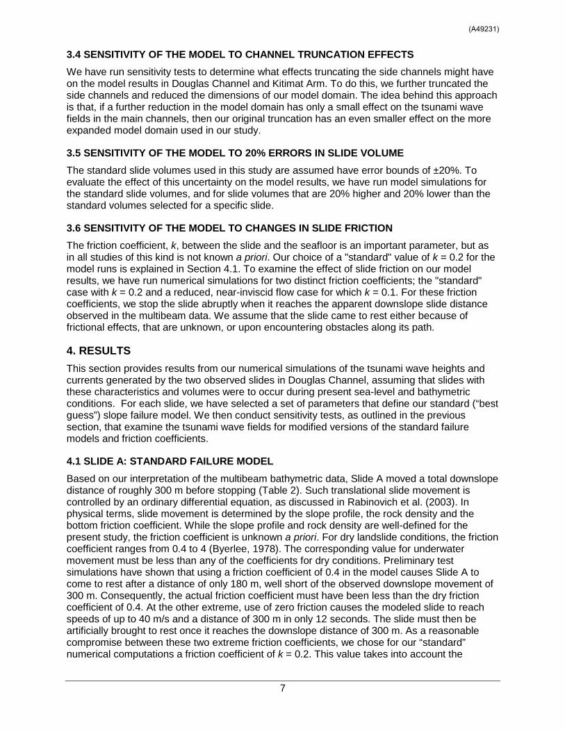
The friction coefficient, k, between the slide and the seafloor is an important parameter, but as in all studies of this kind is not known a priori. Our choice of a "standard" value of k = 0.2 for the model runs is explained in Section 4.1. To examine the effect of slide friction on our model results, we have run numerical simulations for two distinct friction coefficients; the "standard" case with k = 0.2 and a reduced, near-inviscid flow case for which k = 0.1. For these friction coefficients, we stop the slide abruptly when it reaches the apparent downslope slide distance observed in the multibeam data. We assume that the slide came to rest either because of frictional effects, that are unknown, or upon encountering obstacles along its path.

4. RESULTS

This section provides results from our numerical simulations of the tsunami wave heights and currents generated by the two observed slides in Douglas Channel, assuming that slides with these characteristics and volumes were to occur during present sea-level and bathymetric conditions. For each slide, we have selected a set of parameters that define our standard (“best guess”) slope failure model. We then conduct sensitivity tests, as outlined in the previous section, that examine the tsunami wave fields for modified versions of the standard failure models and friction coefficients.

4.1 SLIDE A: STANDARD FAILURE MODEL

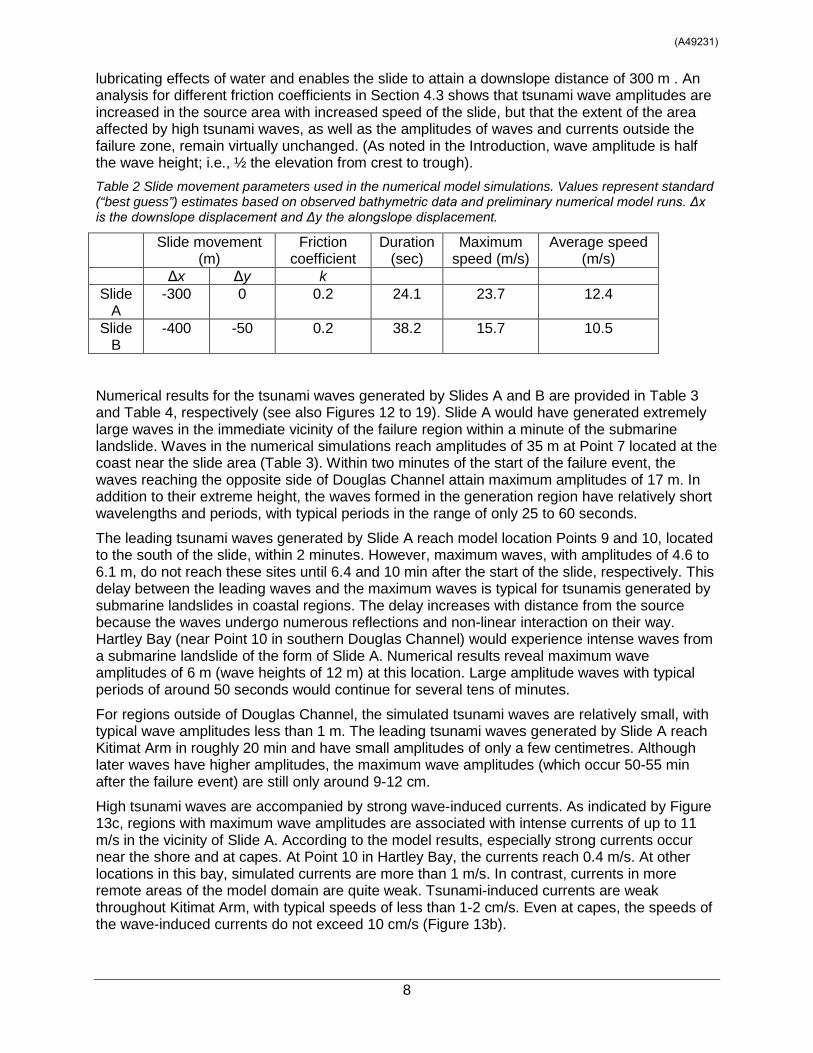
Based on our interpretation of the multibeam bathymetric data, Slide A moved a total downslope distance of roughly 300 m before stopping (Table 2). Such translational slide movement is controlled by an ordinary differential equation, as discussed in Rabinovich et al. (2003). In physical terms, slide movement is determined by the slope profile, the rock density and the bottom friction coefficient. While the slope profile and rock density are well-defined for the present study, the friction coefficient is unknown a priori. For dry landslide conditions, the friction coefficient ranges from 0.4 to 4 (Byerlee, 1978). The corresponding value for underwater movement must be less than any of the coefficients for dry conditions. Preliminary test simulations have shown that using a friction coefficient of 0.4 in the model causes Slide A to come to rest after a distance of only 180 m, well short of the observed downslope movement of 300 m. Consequently, the actual friction coefficient must have been less than the dry friction coefficient of 0.4. At the other extreme, use of zero friction causes the modeled slide to reach speeds of up to 40 m/s and a distance of 300 m in only 12 seconds. The slide must then be artificially brought to rest once it reaches the downslope distance of 300 m. As a reasonable compromise between these two extreme friction coefficients, we chose for our “standard” numerical computations a friction coefficient of k = 0.2. This value takes into account the

(A49231)

8

lubricating effects of water and enables the slide to attain a downslope distance of 300 m . An analysis for different friction coefficients in Section 4.3 shows that tsunami wave amplitudes are increased in the source area with increased speed of the slide, but that the extent of the area affected by high tsunami waves, as well as the amplitudes of waves and currents outside the failure zone, remain virtually unchanged. (As noted in the Introduction, wave amplitude is half the wave height; i.e., ½ the elevation from crest to trough).

Table 2 Slide movement parameters used in the numerical model simulations. Values represent standard (“best guess”) estimates based on observed bathymetric data and preliminary numerical model runs. Δx is the downslope displacement and Δy the alongslope displacement.

Slide movement (m)

Friction coefficient

Duration (sec)

Maximum speed (m/s)

Average speed (m/s)

Δx Δy k Slide

A -300 0 0.2 24.1 23.7 12.4

Slide B

-400 -50 0.2 38.2 15.7 10.5

Numerical results for the tsunami waves generated by Slides A and B are provided in Table 3 and Table 4, respectively (see also Figures 12 to 19). Slide A would have generated extremely large waves in the immediate vicinity of the failure region within a minute of the submarine landslide. Waves in the numerical simulations reach amplitudes of 35 m at Point 7 located at the coast near the slide area (Table 3). Within two minutes of the start of the failure event, the waves reaching the opposite side of Douglas Channel attain maximum amplitudes of 17 m. In addition to their extreme height, the waves formed in the generation region have relatively short wavelengths and periods, with typical periods in the range of only 25 to 60 seconds.

The leading tsunami waves generated by Slide A reach model location Points 9 and 10, located to the south of the slide, within 2 minutes. However, maximum waves, with amplitudes of 4.6 to 6.1 m, do not reach these sites until 6.4 and 10 min after the start of the slide, respectively. This delay between the leading waves and the maximum waves is typical for tsunamis generated by submarine landslides in coastal regions. The delay increases with distance from the source because the waves undergo numerous reflections and non-linear interaction on their way. Hartley Bay (near Point 10 in southern Douglas Channel) would experience intense waves from a submarine landslide of the form of Slide A. Numerical results reveal maximum wave amplitudes of 6 m (wave heights of 12 m) at this location. Large amplitude waves with typical periods of around 50 seconds would continue for several tens of minutes.

For regions outside of Douglas Channel, the simulated tsunami waves are relatively small, with typical wave amplitudes less than 1 m. The leading tsunami waves generated by Slide A reach Kitimat Arm in roughly 20 min and have small amplitudes of only a few centimetres. Although later waves have higher amplitudes, the maximum wave amplitudes (which occur 50-55 min after the failure event) are still only around 9-12 cm.

High tsunami waves are accompanied by strong wave-induced currents. As indicated by Figure 13c, regions with maximum wave amplitudes are associated with intense currents of up to 11 m/s in the vicinity of Slide A. According to the model results, especially strong currents occur near the shore and at capes. At Point 10 in Hartley Bay, the currents reach 0.4 m/s. At other locations in this bay, simulated currents are more than 1 m/s. In contrast, currents in more remote areas of the model domain are quite weak. Tsunami-induced currents are weak throughout Kitimat Arm, with typical speeds of less than 1-2 cm/s. Even at capes, the speeds of the wave-induced currents do not exceed 10 cm/s (Figure 13b).

(A49231)

9

4.2. SLIDE B: STANDARD FAILURE MODEL

Our analysis for Slide B follows the same procedure as for Slide A. An examination of the bathymetric data shows that Slide B moved roughly 400 m before stopping (Table 2). Because Slide B began its movement at greater depth than Slide A, the centre of mass of Slide B underwent a smaller vertical displacement than Slide A. This, in turn, caused Slide B to move significantly slower than Slide A, leading to differences in the simulated tsunami waves generated by the two slides.

Properties of the numerically simulated tsunami waves generated by Slide B are provided in Table 4 and Figures 15 to 19. Slide B would have generated large waves in the vicinity of the failure region. Simulated waves reach the coast adjacent to the slide region within a minute of the failure event, with wave amplitudes of 9.7 m at Point 9 (Table 4). The waves also hit the opposite site of the channel within a minute of the failure event and then take an additional minute to reach Hartley Bay, where waves reach amplitudes of 15.4 m (Point 10). The highest waves to reach Hartley Bay have periods of 52 sec. Powerful oscillations in the bay last for tens of minutes. Waves with high amplitudes (more than 2 m) also occur in the southern part of Douglas Channel and in certain locations of Verney Passage (see Figure 19). At Points 7 and 8, located to the north of the source region, the waves arrive 2.3 and 2.2 min, respectively, after the start of Slide B. Maximum waves with amplitudes of 3.8 m and 1.8 m hit Points 7 and 8 about 10.8 min and 5.8 min after the start of the failure, respectively.

In Verney Passage and in other areas away from the confines of southern Douglas Channel, the tsunami waves are much smaller, with typical amplitudes of less than 0.5 m. The leading tsunami waves reach Kitimat Arm 22 min after the start of the slide, while maximum waves with amplitudes of 8 to 30 cm, reach Kitimat Arm 45 to 60 min after the start of the failure event. We note that the tsunami waves generated by Slide B that impact Kitimat Arm, although still of low amplitude, are somewhat higher than those generated by Slide A despite the fact that Slide B is located further to the south and generates less energetic waves in the source region than Slide A. This seeming paradox is explained by the slower motion of Slide B, which causes it to generate more wave energy in the low frequency band than Slide A. Due to their reduced scattering and reflection, the relatively long and lower frequency waves generated by Slide B propagate more readily through the complex fjord system than the relatively short and higher frequency waves generated by Slide A.

Tsunami waves generated by slide B in the failure region are accompanied by intense currents, with maximum velocities centred in the source area (Figure 17). Because Slide B generated less energetic tsunami waves than Slide A, current speeds in the source area are generally less than those generated by Slide A. In Hartley Bay, currents reach 3 m/s and exceed 4 m/s in the narrow channel to the south of the bay. At Point 9, near the slide zone, current speeds reach 2 m/s. In the source region and at selected capes, the currents can be as strong as 6 m/s.

For sites outside the Douglas Channel and in adjoining channels, the tsunami-induced currents are quite weak. Although currents generated in Kitimat Arm by Slide B are slightly stronger than for Slide A, the currents are still weaker than 10 cm/s (specifically, 1 cm/s at Point 1 and 3 cm/s at Point 2, near the site of the proposed Enbridge facilities).

(A49231)

10

Table 3 Principal tsunami wave statistics for specific locations in the model domain for Slide A.

Point number

Arrival time (min)

Maximum wave amplitude (m)

Time of maximum

(min)

Typical period (sec)

Maximum current speed (m/s)

1 21.7 0.12 54.2 87.0 0.007 2 19.7 0.09 49.7 71.0 0.017 3 15.5 0.45 49.1 68.7 0.092 4 7.5 0.78 20.0 63.0 0.116 5 15.9 0.19 46.2 61.7 0.031 6 17.5 0.24 49.0 69.7 0.023 7 0.0 35.15 0.7 58.3 3.041 8 0.7 16.88 1.8 26.7 2.852 9 2.0 4.61 6.4 77.7 0.761 10 2.2 6.14 9.9 49.3 0.516 11 8.8 0.61 26.8 58.0 0.042 12 8.2 0.34 30.1 71.7 0.018 13 11.6 0.06 33.9 65.3 0.006 14 14.1 0.04 42.3 70.7 0.002 15 19.0 0.01 53.1 111.0 0.003

Table 4 Principal tsunami wave statistics for specific locations in the model domain for Slide B.

Point number

Arrival time (min)


Time of maximum

(min)



1 24.5 0.28 59.1 95.0 0.013 2 22.5 0.08 45.5 89.0 0.029 3 18.3 0.38 28.5 85.0 0.058 4 10.3 0.77 22.1 99.7 0.059 5 18.8 0.21 53.2 85.3 0.037 6 14.8 0.28 43.1 63.0 0.040 7 2.3 3.87 10.8 56.7 0.553 8 2.2 1.84 5.8 95.0 0.640 9 0.1 9.74 0.9 51.7 1.945 10 1.0 15.42 2.4 52.7 1.155 11 6.1 0.84 44.2 67.3 0.040 12 5.5 0.49 24.4 68.0 0.027 13 8.9 0.12 50.2 125.7 0.007 14 11.9 0.06 39.9 79.7 0.006 15 16.8 0.02 57.4 120.7 0.008

4.3 SENSITIVITY ANALYSES

This section discusses the findings of the model sensitivity analyses outlined in Section 3.

4.3.1 Sensitivity to bathymetric smoothing

To estimate the effect of our selective bathymetric smoothing, we have compared the tsunami waves generated by Slide B (standard run, see Section 4.2) and those obtained using a lower

(A49231)

11

degree of bathymetric smoothing, such that 4.0<∆ hh . To quantify the sensitivity of the model to the bathymetric smoothing, we have computed the skill, S, for the distribution of wave amplitude maxima in the study area (i.e., results for Slide B from the standard run versus a test run that uses less smoothed seafloor topography). Here, skill is defined as

2

2)(1

A

AAS n−

−= (4.1)

where A is the distribution of the wave amplitude maxima derived for the standard model run for Slide B and An is the corresponding distribution for the Slide B model run using the less-smooth bathymetric test-case data. In a similar manner, we estimated skill for the maximum velocity values. Among other estimated sensitivity parameters is the correlation, r, between values for the standard and the test runs, as well as the coefficients of linear regression between maximum amplitudes in the model domain (Table 5). The last column in Table 5 contains the root-mean-square deviation (RMSD), which measures the mean discrepancy between the standard model runs and the test runs. These characteristics also were calculated for all subsequent sensitivity tests. As indicated by the statistical comparisons in Table 5, there is a high correlation between the two model runs, confirming that moderate selective smoothing of the bathymetric data has only a minor effect on the tsunami modeling results. Average discrepancy (RMSD) is below 2 cm for the maximum amplitude values and below 1 cm/s for the maximum velocity values (Table 5). A detailed examination of the changes in the wave field (not shown) reveals that the changes are confined to the source region and negligible outside of this region.

4.3.2. Sensitivity to the channel truncation effects

To estimate the effects of the truncated channels on the tsunami waves, we examined results for a truncated model domain (Figure. 11) whose area is only 35.7% that of the original model domain. Channels in the west, east, and south of the original model domain were truncated, but the northern area was left unchanged. Because the areas removed from the primary model domain receive little of the tsunami energy flux from the source regions, there are only minor changes in the modeling results. As confirmed by our modeling results, there is only a small decrease in the tsunami energy in the areas closest to the new model boundaries (because some of the energy is now no longer reflected back from the area we truncated), while for the northern area the results are essentially unchanged. There is a small (~1%) decrease in the mean energy value related to the open boundaries which are now closer to the source for the truncated domain, and, consequently, allow more energy to radiate out of the area.

To further quantify the sensitivity of the model to channel truncation, we compare the wave amplitude and current speed maxima obtained using the standard (pre-truncated) model and the truncated model. All statistical characteristics, including the skill (with S > 99% for both wave amplitude and current speed) indicate that the two model runs are nearly identical (Table 5). We conclude that our truncation of several side channels when formulating the original model domain has little effect on the tsunami model results for the main channels of the coastal waterway.

4.3.3 Sensitivity to changes in slide volume

We expect our model results to be sensitive to slide volume. In the linear theory, the amplitudes of the waves and the wave-induced currents are directly proportional to the slide thickness. In non-linear models, the results are less obvious. To estimate the effect of changes in the slide volume on numerical simulations, we have run two additional tests to examine the tsunami waves generated by Slide B; one for a slide thickness that is 20% greater than the standard

(A49231)

12

model and a second in which the slide volume is 20% lower than the standard model. A comparison of the two test runs against the standard model run for Slide B is presented in Table 5. The correlation between the "standard" model and "thinner" (20% lower volume slide) model is very high (r > 99%) for both wave amplitude maxima and current speed maxima, indicating that nonlinear effects have a minor effect on the numerical output. In the case of a thicker (20% greater volume slide), the correlation between the test run and the standard run is also high, although somewhat less than for the smaller volume case. These results reveal an increase in nonlinear effects with increasing slide thickness.

4.3.3 Sensitivity to changes in slide friction

These sensitivity tests proved to be the most difficult to perform and to analyze, as changes in bottom friction clearly lead to significant changes in the slide dynamics and in downslope speed and timing. Using a reduced, near-inviscid friction coefficient of k = 0.1, we find that Slide B moves 400 m downslope in just 26 sec (i.e. 50% faster than that for the standard model run). As a consequence, it generates higher tsunami waves. Statistical comparison between this test case and the standard run (see Table 5) shows that the correlation coefficient between the maxima wave amplitude and current speed distributions for two runs remains high but that the skill is relatively low (r = 62% for the wave amplitude maxima fields). The relatively low skill is related to a ~50% increase in tsunami wave amplification for the more rapidly moving lower friction slide in comparison with the standard run.

To estimate how this amplification is distributed within the model domain, we calculated the full statistics for the low friction test run (Table 6) for the same 15 location points used for the standard model (Table 4). Comparison of the results in Table 6 with those for the "standard" model in Table 4 shows that, despite the fact that faster low friction slide generated much higher waves, the wave statistics for the lower friction test case are generally very close (typically within 10%) of those obtained using the "standard" model. The major differences are localized in the central zone (Points 7, 8, 9, and 10) where the lower friction test run generated much higher (40-90%) waves. This is because the rapidly moving slide generates more energy in the high-frequency wave band but essentially the same amount of energy in the low-frequency wave band as the slower moving standard slide. For the test case, the high-frequency waves are amplified significantly in the source area, but, because these waves do not propagate to remote locations in the model domain, the distribution of wave energy farther than a few kilometres from the source remains almost unchanged. This is an important finding since it demonstrates that, although localized wave amplitudes depend on the characteristics of the slide movement, the regional extent of the waterways affected by the submarine landslide generated tsunamis is largely insensitive to the slide speed and, hence, to the slide friction coefficient.

(A49231)

13

Table 5 Sensitivity test results for maximum wave amplitude, A, and maximum speed, v. Regression offset and root-mean-square deviation (RMSD) is in units indicated for each variable.

Test Parameter Skill (%) Correlation (%) Regression RMSD

Slope Offset

Bathymetric smoothing

A (cm) 99.73 99.90 0.97 -0.15 1.76

v (cm/s) 99.55 99.82 0.97 -0.03 0.56

Domain truncation A (cm) 99.78 99.88 0.99 -0.11 2.67

v (cm/s) 99.75 99.87 0.99 -0.02 0.69

+20% slide volume A (cm) 96.30 99.26 0.84 0.09 6.57

v (cm/s) 93.36 97.11 0.84 0.02 2.14

-20% slide volume A (cm) 95.73 99.54 1.17 0.10 7.05

v (cm/s) 94.55 99.61 1.21 0.00 1.94

Slide friction A (cm) 62.08 98.01 1.54 -1.15 21.01

v (cm/s) 56.67 97.71 1.57 -0.29 5.46

Table 6 Tsunami wave statistics for specific locations in the model domain for Slide B. Values are derived using a reduced friction coefficient k = 0.1.

Point number

Arrival time (min)


Time of maximum

(min)



1 24.4 0.29 59.1 95.0 0.013 2 22.4 0.09 50.8 95.0 0.030 3 18.3 0.42 28.4 84.3 0.061 4 10.3 0.85 22.0 103.0 0.064 5 18.7 0.22 36.5 89.0 0.038 6 14.8 0.33 38.4 55.7 0.046 7 2.2 5.26 10.7 50.0 0.836 8 2.1 2.34 5.7 49.7 0.867 9 0.1 19.21 0.8 37.7 2.953 10 0.9 24.66 2.3 53.7 2.072 11 6.0 0.98 44.1 66.7 0.067 12 5.4 0.58 24.3 66.0 0.042 13 8.8 0.14 25.0 81.0 0.008 14 11.9 0.06 39.8 77.7 0.006 15 16.8 0.02 573 121.0 0.008

5. DISCUSSION

The primary results presented in Section 4 can be summarized by a simple empirical analysis based on the model results. Depending on the level of bottom friction, the slides move downslope with a peak velocity, Vslide, of around 25 m/s and terminate, after moving a distance of around 300 m, after a duration, Tslide, of roughly 30 seconds. This rapid failure and

(A49231)

14

subsequent abrupt stop generates tsunami waves with amplitudes of up to 30 m, wavelengths λ

~ c × Tslide of around 2 km, and periods, Ttsunami, ~ Tslide. Here, gHc = ~ 65 m/s is the tsunami

propagation speed for mid-channel water depth H ~ 400 m; g ~ 9.8 m/s2 is the acceleration of gravity.

Maximum wave heights occur along the shorelines adjacent to and directly opposite from the failure region. As clearly indicated by the tsunami model results, it is the sudden stop of the slide motion near the base of the channel slope and the high Froude number response of the water surface that releases the forced wave to become a high-amplitude free wave. If the slide slows down to a gradual stop, rather than stopping suddenly (when the slide velocity would be high), the Froude number would be smaller, the forced water surface distortion smaller, and the amplitude of the subsequent free waves reduced. (The Froude number is the ratio Fr = Vslide,/c < 1, where Vslide is the slide speed and c is the phase speed of free waves). Thus, the greater the Froude number the greater the height of the forced waves.

According to the model results, the waves generated by the two submarine landslides decay rapidly to the south and north of the source regions due to geometric spreading, scattering, and frictional affects within the channel. The relatively short wavelengths of the landslide-generated tsunami waves are a major factor contributing to the rapid along-channel decay in wave amplitudes. A detailed analysis of our numerical results reveals that short tsunami waves traveling northward along Douglas Channel from the source regions have considerable difficulty negotiating the 50 degree right-hand turn located midway along Douglas Channel, opposite Gertrude Point on the central western coast of Hawkesbury Island. Only the longer wavelength components of the wave field can refract and reflect around the sharp corner and propagate toward Kitimat Arm. Most of the energy associated with the shorter waves is reflected back to the south where it helps to maintain the persistently high waves which reverberate for hours in the southern area of Douglas Channel. The low wave heights simulated for Kitimat Arm are due to the relatively low amplitudes of these longer wave components.

Figure 20 shows the maximum tsunami wave amplitudes and current speeds for the two slides in the immediate vicinity of the slides. We designated each of these general areas in terms of specific tsunami zoning (Figures 15 and 19), which partitions the regions according to their tsunami wave heights and current speeds. Regions with highest wave heights and current speeds would likely present significant risks to any marine traffic through the channel during a period of strong tsunami wave activity.

The two slides show remarkable similarity in their tsunami zoning as represented by the spatial distributions of wave height and current maxima. This is probably not surprising given that channel depths and profiles, and the overall dimensions of the slides, are comparable. For wave heights, we observe three main regions where the waves are relatively large: in the immediate area of each slide (the source region), in the middle of the channel, and near the opposite shore. For current speeds, there are two main regions of dangerous currents: an area extending from each slide to approximately the middle of the channel, and a narrower strip of water adjacent to the opposite shore. Wave heights and currents are also large at other near shore locations in relatively close proximity to tsunami zoning; in particular, off some of the capes and inside smaller bays which tend to funnel the incoming tsunami wave energy.

Some differences in the wave amplitudes and currents for the two slides arise from different responses to the bathymetry and coastline, but there are also quantitative differences in the initial forcing for the two slides. As explained in Sections 4.1 and 4.2, Slide A moved a shorter distance with more acceleration and had to stop more suddenly than Slide B, creating larger waves and stronger currents. This difference is reflected in the different scales (colour bar) presented in the top and bottom panels of Figure 20.

(A49231)

15

According to the results shown in Figures 15, 19 and 20, we conclude that for Slide A, the largest tsunami waves (those with amplitudes greater than 2 m) would be observed in the region extending from the southern part of Douglas Channel to the 50° channel bend (Figure 15). For Slide B, such waves occur in the southern part of the channel, including the nearby coastlines of Verney Passage and the northern coast of Gil Island (Figure 19). In more remote regions of the inner coastal waterway, the modelled tsunami waves have peak amplitudes of less than 2 m. Most waves have amplitudes well below 1 m.

Based on our sensitivity experiments, it is clear that the model results are not overly sensitive to smoothing of the gridded bathymetry, or to truncation of the area used in the model domain (green box in Figure 11). However, changing the friction coefficient, k, leads to more complex effects. When we decreased k to 0.1, wave amplitudes near the source increased significantly, while the amplitudes in more distant areas were virtually unchanged. We have also determined that the wave amplitudes and current speeds derived by the model are almost directly proportional to the volume of the slides. The more slowly moving Slide B generated longer wave periods and wavelengths than Slide A, and therefore marginally higher tsunami waves and currents in more remote regions of the model domain.

6. CONCLUSIONS

The two massive (~65 million cubic meter) submarine landslides discovered recently in Douglas Channel likely produced large tsunami waves in the channel during their occurrence sometime in the early to mid-Holocene. If similar submarine slides were to occur again somewhere in the same general area, they could present a significant risk to navigation and to nearby shore installations and coastal communities. We investigate this risk using a nonlinear, non-hydrostatic numerical model which simulates the waves that would have been generated by the observed slides were they to occur under the bathymetric conditions that presently exist in Douglas Channel.

Based on the multibeam data recently collected by the Canadian Hydrographic Service and Natural Resources Canada, the slides moved a distance of roughly 300 to 400 m before stopping near the base of the slope in water depths of around 400 m. Graphic reconstruction of the slide regions immediately prior to failure indicates the slides were wedge-shaped. The head of the more northern slide (Slide A) began at a depth of around 60 to 100 m, while that of the more southern slide (Slide B) at a depth of 75 to 120 m. Depending on the friction between the slide and the underlying seafloor, the slides would have moved downslope with a peak velocity of ~25 m/s before coming to rest after a duration of about 30 seconds. The numerical simulations show that submarine landslides with these characteristics would generate tsunami waves with peak amplitudes of 30 to 40 m, current speeds of up to 15 m/s (near 30 knots), have wavelengths of the order of 1-2 km, and wave periods of tens of seconds to several minutes.

Highest waves and strongest currents would occur along the shoreline opposite and adjacent to the failure regions. Because of their relatively short wavelengths, the tsunami waves undergo multiple reflections and a high degree of scattering from the complex shoreline and bathymetry in Douglas Channel. These effects, combined with the flux of tsunami energy through adjoining waterways and channels, cause rapid attenuation of the waves with distance south and north of the source region. At the estimated propagation speeds of ~65 m/s, it takes roughly 10 to 15 minutes for the simulated waves to propagate approximately 40 to 45 km to the intersection of Douglas Channel and Kitimat Arm, where peak wave amplitudes would be diminished to less than 1 m. It takes another 15 minutes for the waves to reach sites near the proposed Enbridge facilities in Kitimat Arm where wave amplitudes would be reduced to a few tens of centimetres and associated currents to speeds less than a few tens of centimetres per second.

As for other tsunami generation processes, the highest waves and strongest currents in any particular region of this coastal waterway would occur near the shoreline. Based on the

(A49231)

16

numerical findings, tsunamis generated by submarine landslides of the form identified for the southern end of Douglas Channel would have heights and currents that could have major impacts on the coastline and vessel traffic at the time of the event throughout much of Douglas Channel, but a minor impact on water levels, currents and hence vessel traffic in Kitimat Arm. Hartley Bay, at the southern end of Douglas Channel, would be impacted by high waves and strong currents, whereas Kitimat, at the northern end of Kitimat Arm, would experience negligible wave effects. In particular, Slide B, the larger of the two slides, generates somewhat lower waves and weaker currents in the failure region than Slide A, but higher waves and stronger currents in more distant regions of the model domain than Slide A. It is the slower downslope motion of Slide B and resulting longer ensuing tsunami wavelengths that are responsible for both of these effects. Other factors, such as contributions from subaerial components of slides, which we have not addressed in this study, could also modify significantly the wave fields in regions adjacent to, or remote from, the slide region. Additional modeling would be required to assess the characteristics of possible tsunamis originating beyond the area of the two identified slope failures. Further studies also are needed to examine the sensitivity of the numerical results to specific model formulation, seafloor topography, bottom friction, and other physical factors, and to examine tsunami wave resonances and the attenuation time scales for the tsunami wave fields.

ACKNOWLEDGEMENTS

We thank Robert Kung of Natural Resources Canada for his helping with the slide model formulation and Drs. Vaughn Barrie and Bill Crawford for their constructive reviews of the penultimate version of the report. Earth Sciences Sector Contribution Number 20120303.

REFERENCES

Bornhold, B.D. and Thomson, R.E. 2012. Tsunami hazard assessment related to slope failures in coastal waters. Chapter 10 in Landslides - Types, Mechanisms and Modeling, Eds. J. Clague and D. Stead; Cambridge University Press.

Bornhold, B.D., Harper, J.R., McLaren, D. and Thomson, R.E. 2007. Destruction of the First Nations Village of Kwalate by a rock avalanche‐generated tsunami. Atmosphere-Ocean, 45(2), 123-128.

Byerlee, J.D. 1978. Friction of rocks. Pure and Applied Geophysics, 116 (4–5), 615–626, doi:10.1007/BF00876528.

Conway, K.W., Barrie, J.V. and Thomson, R.E. 2012. Submarine slope failures and tsunami hazard in coastal British Columbia: Douglas Channel and Kitimat Arm. Geological Survey of Canada, Current Research 2012-10, 13 p., doi:10.4095/291732.

Jiang, L. and LeBlond, P.H. 1992. The coupling of a submarine slide and the surface waves which it generates. J. Geophys. Res., 97(C8), 12,731–12,744, doi:10.1029/92JC00912.

Fine, I.V., Rabinovich, A.B., Thomson, R.E. and Kulikov, E.A. 2003. Numerical Modeling of Tsunami Generation by Submarine and Subaerial Landslides. In: Submarine Landslides and Tsunamis, Eds. Ahmet C. Yalciner, Efim Pelinovsky, Costas E. Synolakis, and Emile Okal. Kluwer Academic Publishers, Netherlands, pp. 69-88.

Kowalik, Z., Knight, W., Logan, T. and Whitmore, P. 2005. Numerical modeling of the global tsunami: Indonesian Tsunami of 26 December 2004. Science of Tsunami Hazards, 23(1), 40–56.

Krige, D. G. 1966. Two-dimensional weighted moving average trend surfaces for ore valuation. Journal of the South African Institute of Mining and Metallurgy, 67, 13-38.

(A49231)

17

Mosher, D.M. 2009. Submarine landslides and consequent tsunamis in Canada. Geoscience Canada, 36(4), 179-190.

Murty, T.S. 1979. Submarine slide-generated water waves in Kitimat Inlet, British Columbia. J. Geophys. Res., 84(C12), 7777–7779, doi:10.1029/JC084iC12p07777.

Rabinovich, A.B., Thomson, R.E., Kulikov, E.A., Bornhold, B.D. and Fine, I.V. 1999. The landslide-generated tsunami of November 3, 1994 in Skagway Harbor, Alaska: A case study. Geophys. Res. Lett., 26 (19), 3009-3012.

Rabinovich, A.B., Thomson, R.E., Bornhold, B.B., Fine, I.V. and Kulikov, E.A. 2003. Numerical modelling of tsunamis generated by hypothetical landslides in the Strait of Georgia, British Columbia. Pure and Applied Geophysics, 160, 1273-1313.

Roddick, J.A. 1970. Douglas Channel-Hecate Strait map-area, British Columbia, (103H). Geological Survey of Canada, Paper 70-41, 56p.

ROMSTOOLS: http://www.romsagrif.org. Accessed on 25 October 2012.

Skvortsov, A. and Bornhold, B. 2007. Numerical simulation of the landslide-generated tsunami in Kitimat Arm, British Columbia, Canada, 27 April 1975. J. Geophys. Res., 112, F02028, doi:10.1029/2006JF000499.

Stelling, G.S. and Duinmeijer, S.P.A. 2003. A staggered conservative scheme for every Froude number in rapidly varied shallow water flows. International Journal for Numerical Methods in Fluids, 43(12), 1329–1354.

Stelling, G.S. and Zijlema, M. 2003. An accurate and efficient finite-difference algorithm for non-hydrostatic free-surface flow with application to wave propagation. International Journal for Numerical Methods in Fluids, 43(1), 1–23.

Thomson, R.E., Rabinovich, A.B., Kulikov, E.A., Fine, I.V. and Bornhold, B.D. 2001. On numerical simulation of the landslide-generated tsunami of November 3, 1994 in Skagway Harbor, Alaska. In: Tsunami Research at the End of a Critical Decade, Ed. G. Hebenstreit; Kluwer, Dorderecht, 243-282.

Yamazaki, Y., Kowalik, Z., and Cheung, K. F. 2008. Depth-integrated, non-hydrostatic model for wave breaking and run-up. International Journal for Numerical Methods in Fluids, DOI: 10.1002/fld.1952.

Yamazaki, Y., Kowalik, Z., and Cheung, K. F. 2010. Depth-integrated, non-hydrostatic model with grid nesting for tsunami generation, propagation, and run-up. International Journal for Numerical Methods in Fluids, DOI: 10.1002/fld.2485.

(A49231)

http://www.romsagrif.org/

18

FIGURES

Figure 1 The study region. The general region of study is shown in the inset. Slides A and B are located within the red boxes shown in the main figure. Gertrude Point marks a major right-hand turn in the channel orientation toward the northeast.

(A49231)

19

Figure 2 Detailed multibeam imagery of (a) Slide A and (b) Slide B. Plotted to the left of each slide are numbered bathymetric profiles extracted from multibeam bathymetry; locations for each profile are shown in the slide image. From Conway et al. (2012).

(A49231)

20

Figure 2. Continued.

(A49231)

21

Figure 3 Side view of land elevations (positive values) and water depth (negative values) in the region of submarine landslides A and B. The bathymetric data provided by Natural Resources Canada have been gridded at 5-m resolution; land elevations are SRTM 3' data (http://earthexplorer.usgs.gov). The solid red line denotes the Lower Water sea level (Canadian Hydrographic Service).

(A49231)

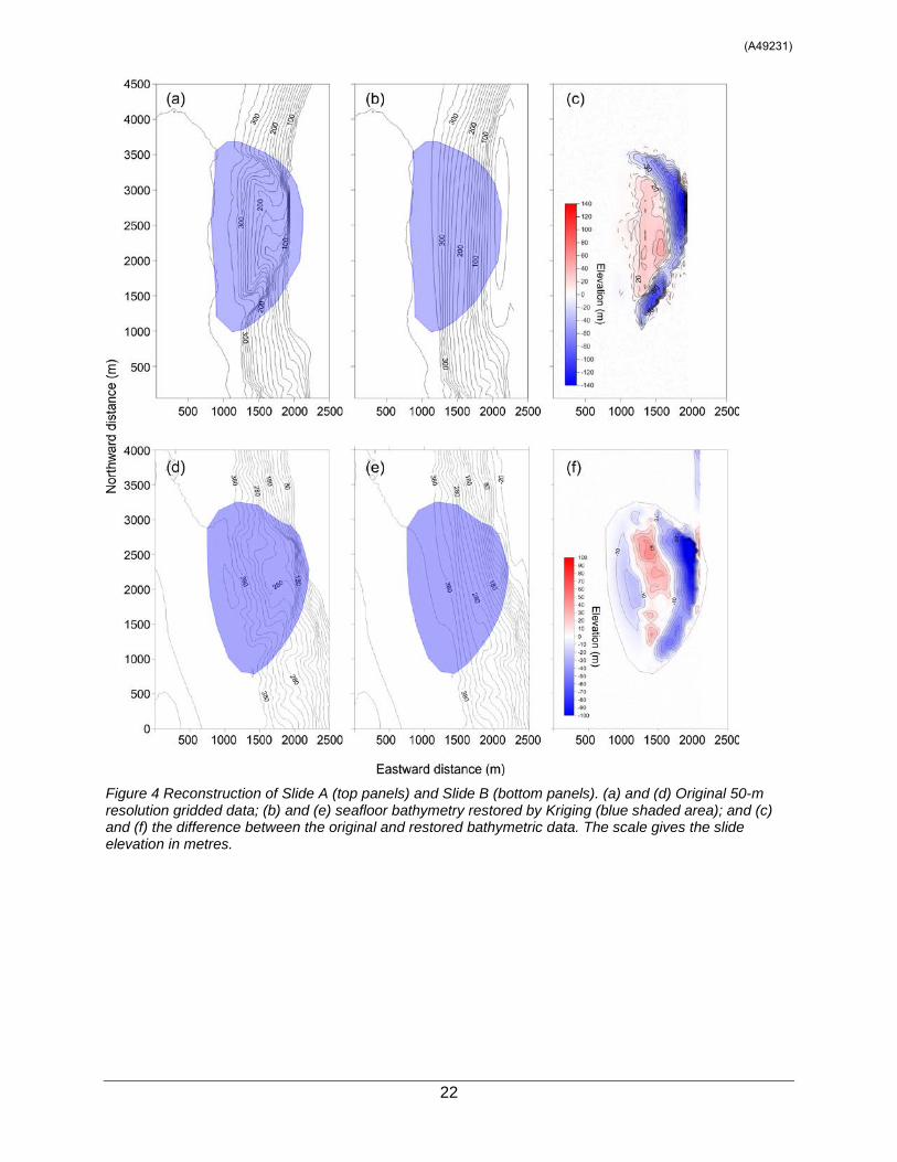
22

Figure 4 Reconstruction of Slide A (top panels) and Slide B (bottom panels). (a) and (d) Original 50-m resolution gridded data; (b) and (e) seafloor bathymetry restored by Kriging (blue shaded area); and (c) and (f) the difference between the original and restored bathymetric data. The scale gives the slide elevation in metres.

(A49231)

23

Figure 5 Reconstruction of Slide A (top panels) and Slide B (bottom panels). (a) and (c) Observed bathymetry; and (b) and (d) the slide body generated on the basis of Kriging. Depths and slide elevations are in metres.

(A49231)

24

Figure 6 Reconstruction of Slide A (top panels) and Slide B (bottom panels). From left to right: The restored seafloor topography immediately prior to failure (the dotted line outlines the slide region); the initial position of the block slide, followed by the downslope shifted final position of the block slide after it has come to rest (the initial position of the slide is shown with the dotted line for a reference); at its final position on the present day seafloor (right hand panel), the slide body had shifted 300 m for Slide A and 400 m for Slide B westward (downslope) relative to its original position. Slide B also had a southward component of 50 m in its shift vector.

(A49231)

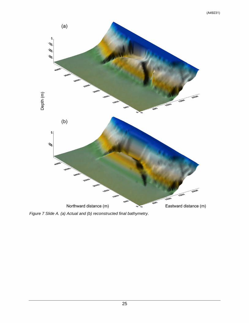
25

Figure 7 Slide A. (a) Actual and (b) reconstructed final bathymetry.

(A49231)

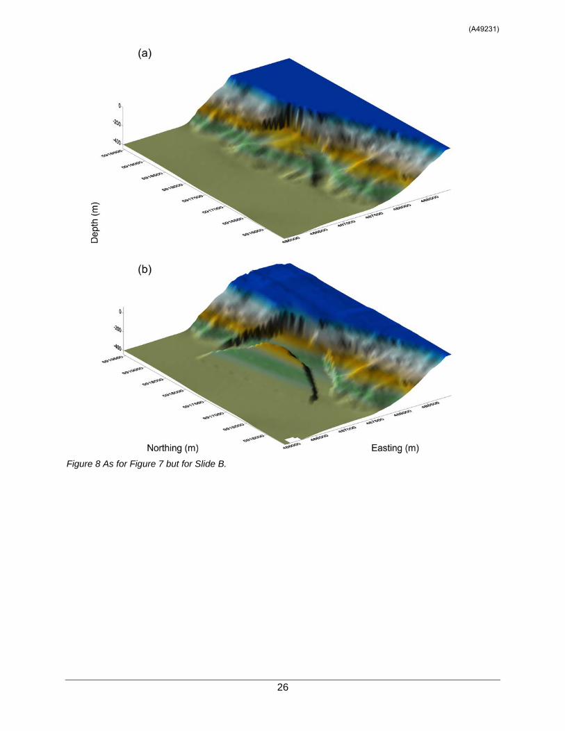
26

Figure 8 As for Figure 7 but for Slide B.

(A49231)

27

Figure 9 Bathymetry (blue) and LW coastline (red) data coverage. The 50-m resolution bathymetric data were provided by the Canadian Hydrographic Service. The yellow boundary denotes the outer boundary of the numerical model domain.

(A49231)

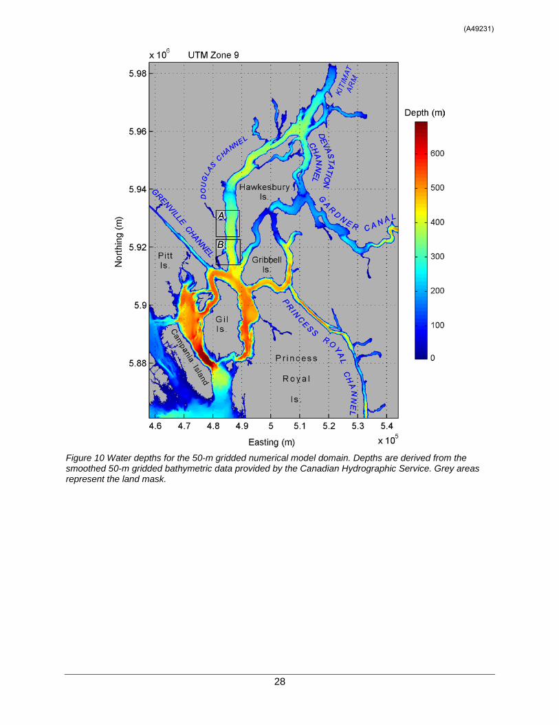
28

Figure 10 Water depths for the 50-m gridded numerical model domain. Depths are derived from the smoothed 50-m gridded bathymetric data provided by the Canadian Hydrographic Service. Grey areas represent the land mask.

(A49231)

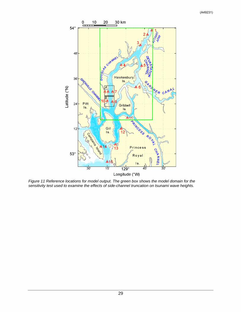
29

Figure 11 Reference locations for model output. The green box shows the model domain for the sensitivity test used to examine the effects of side-channel truncation on tsunami wave heights.

(A49231)

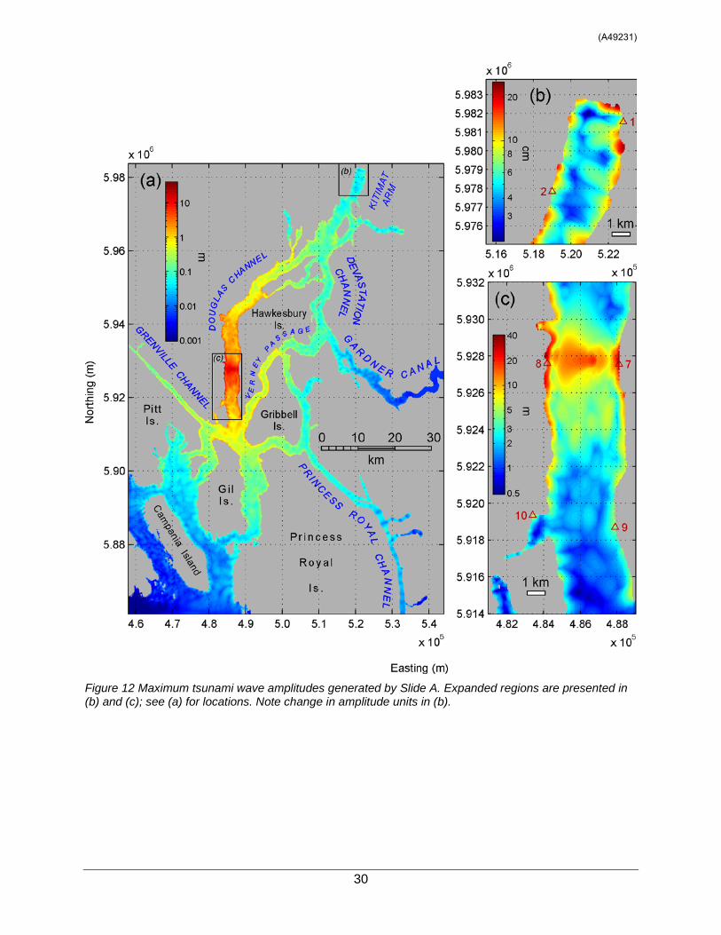
30

Figure 12 Maximum tsunami wave amplitudes generated by Slide A. Expanded regions are presented in (b) and (c); see (a) for locations. Note change in amplitude units in (b).

(A49231)

31

Figure 13 Maximum current speeds generated by Slide A. Expanded regions are presented in (b) and (c); see (a) for locations. Note change in velocity units in (b).

(A49231)

32

Figure 14 Simulated tsunami wave amplitudes as functions of time at the reference locations (see Figure 11) for Slide A. Location number is indicated to the left of each group of series. Note the different time and wave amplitude scales for the central locations, as well as the different amplitude scale for Points 13 to 15.

(A49231)

33

Figure 15 Tsunami zoning based on the maximum simulated tsunami wave amplitudes for Slide A.

(A49231)

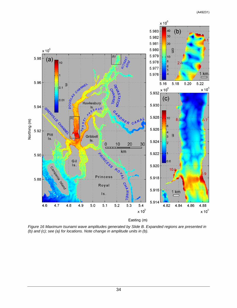
34

Figure 16 Maximum tsunami wave amplitudes generated by Slide B. Expanded regions are presented in (b) and (c); see (a) for locations. Note change in amplitude units in (b).

(A49231)

35

Figure 17 Maximum current speeds generated by Slide B. Expanded regions are presented in (b) and (c); see (a) for locations. Note change in velocity units in (b).

(A49231)

36

Figure 18 Simulated tsunami wave amplitudes as functions of time at the reference locations (see Figure 11) for Slide B. Location number is indicated to the left of each group of series. Note the different time and wave amplitude scales for the central locations, as well as the different amplitude scale for Points 13 to 15.

(A49231)

37

Figure 19 Tsunami “zoning” based on the maximum simulated tsunami wave amplitudes for Slide B.

(A49231)

38

Figure 20 Maximum tsunami wave amplitudes and current speeds in the source region; see area (c) in Figures 12, 13, 16, and 17.

(A49231)

i+ i - ceaa-acee.gc.ca · pdf filecolumbia to markets in china and california with tankers of...

Documents