hypothesis testing - brown university · 11.3 research hypothesis testing… the fda or...

Hypothesis Testing

Chap 10-1Statistics for Business and Economics, 6e © 2007 Pearson Education, Inc.

11.2

Nonstatistical Hypothesis Testing…

In a trial a jury must decide between two hypotheses. n H0: The null hypothesis - The defendant is

innocentn H1: The alternative hypothesis -The defendant

is guiltyThe jury does not know which hypothesis is true. They must make a decision on the basis of evidence presented.

11.3

Research Hypothesis Testing…

The FDA or “science” needs to decide on a new theory, drug, treatment…nH0: The null hypothesis - the current theory, drug, treatment, is as good or betternH1: The alternative hypothesis - the new theory, drug, treatment, should replace the old oneResearchers do not know which hypothesis is true. They must make a decision on the basis of evidence presented.

11.4

Hypothesis Testing Terms

n Convicting the defendant is rejecting the null hypothesis in favor of the alternative hypothesis.

n There is enough evidence to conclude that the defendant is guilty (i.e., there is enough evidence to support the alternative hypothesis).

n If the jury acquits it is stating that there is not enough evidence to support the alternative hypothesis.

n The jury is not saying that the defendant is innocent, only that there is not enough to convict.

n We don’t accept the null hypothesis, we just don’t have sufficient evidence to reject it.

11.5

Hypothesis Testing…

n Two hypotheses, the null and the alternative n Begins with the assumption that the null hypothesis is

true.n Is there enough evidence to infer that the alternative

hypothesis is true, or the null is not likely to be true.n There are two possible decisions:

n Enough evidence to support the alternative hypothesis. Reject the null.

n Not enough evidence to support the alternative hypothesis. Fail to reject the null.

Example: Is the Coin Biased?

n Flip a coin 10 times and get 2 HEAdsn Flip a coin 100 times and get 20 HEAdsn Flip a coin 100 times and get 37 HEAdsn Flip a coin 100 times and get 47 HEAds

Statistics for Business and Economics, 6e © 2007 Pearson Education, Inc. Chap 10-6

We reject the prior assumption that the coin is unbiased if the number of HEADs is very unlikely under that assumption


n H0 : Probability of HEAD = ½n Possible alternatives:

n H1 : Probability of HEAD ≠ ½n H1 : Probability of HEAD is > ½n H1 : Probability of HEAD is < ½



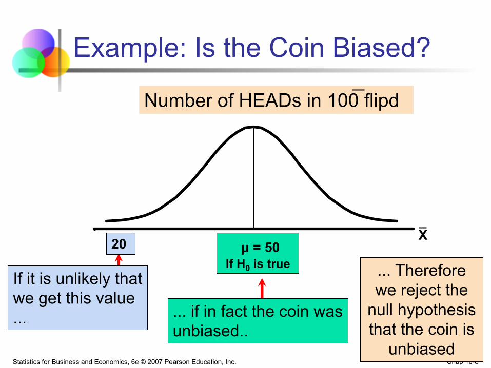
Number of HEADs in 100 flipd

μ = 50If H0 is true

If it is unlikely that we get this value ...

... Therefore we reject the

null hypothesis that the coin is

unbiased


20

... if in fact the coin was unbiased..

X


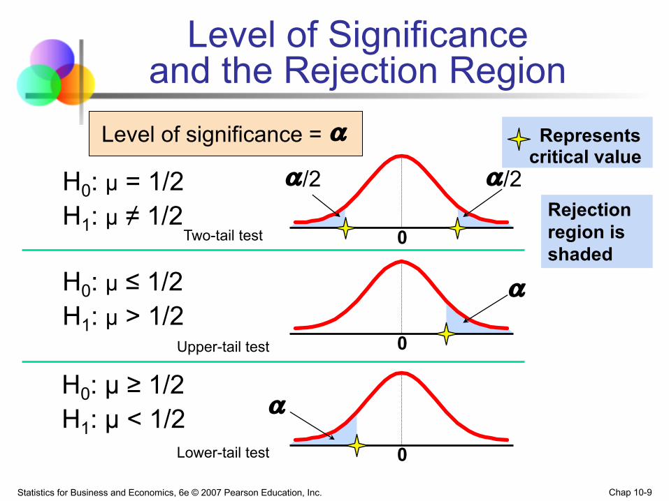
Level of Significance and the Rejection Region

H0: μ ≥ 1/2 H1: μ < 1/2

0

H0: μ ≤ 1/2 H1: μ > 1/2

a

a

Representscritical value

Lower-tail test

Level of significance = a

0Upper-tail test

Two-tail testRejection region is shaded

/2

0

a/2aH0: μ = 1/2 H1: μ ≠ 1/2


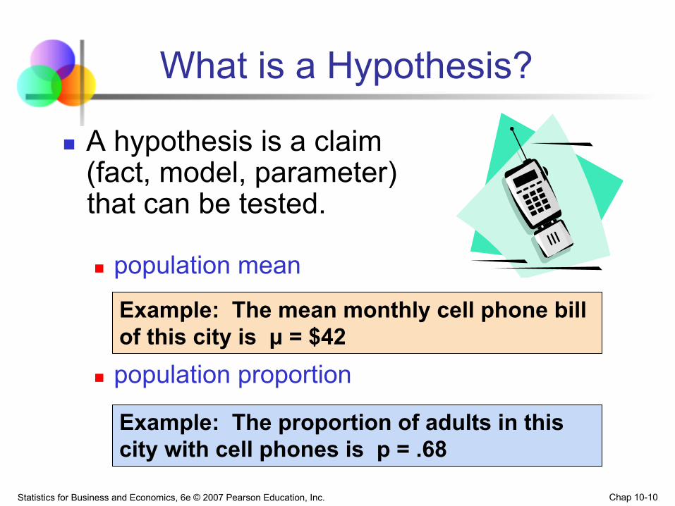
What is a Hypothesis?

n A hypothesis is a claim (fact, model, parameter) that can be tested.

n population mean

n population proportion

Example: The mean monthly cell phone bill of this city is μ = $42

Example: The proportion of adults in this city with cell phones is p = .68


The Null Hypothesis, H0

n States the assumption (numerical) to be testedExample: The average number of TV sets in

U.S. Homes is equal to three ( )

n Is always about a model, not about a sample statistic

3μ:H0 =

3μ:H0 = 3X:H0 =

Statistics for Business and Economics, 6e © 2007 Pearson Education, Inc.

Population

Claim: thepopulationmean age is 50.(Null Hypothesis:

REJECT

Supposethe samplemean age is 20: X = 20

SampleNull Hypothesis

20 likely if μ = 50?=Is

Hypothesis Testing Process

If not likely,

Now select a random sample

H0: μ = 50 )

X


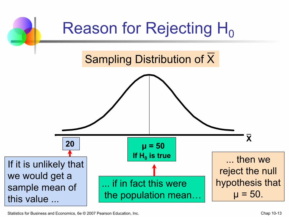
Sampling Distribution of X

μ = 50If H0 is true

If it is unlikely that we would get a sample mean of this value ...

... then we reject the null

hypothesis that μ = 50.

Reason for Rejecting H0

20

... if in fact this werethe population mean…

X


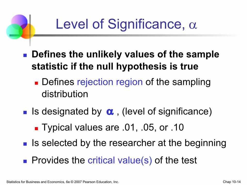
Level of Significance, a

n Defines the unlikely values of the sample statistic if the null hypothesis is truen Defines rejection region of the sampling

distribution

n Is designated by a , (level of significance)n Typical values are .01, .05, or .10

n Is selected by the researcher at the beginning

n Provides the critical value(s) of the test


Level of Significance and the Rejection Region

H0: μ ≥ 3 H1: μ < 3

0

H0: μ ≤ 3 H1: μ > 3

a

a

Representscritical value

Lower-tail test

Level of significance = a

0Upper-tail test

Two-tail testRejection region is shaded

/2

0

a/2aH0: μ = 3 H1: μ ≠ 3


Errors in Making Decisions

n Type I Errorn Reject a true null hypothesisn Considered a serious type of error

The probability of Type I Error is an Called level of significance of the testn Set by researcher in advance


Errors in Making Decisions

n Type II Errorn Fail to reject a false null hypothesis

The probability of Type II Error is β

(continued)


Outcomes and Probabilities

Actual SituationDecisionDo NotReject

H0

No error(1 - )a

Type II Error( β )

RejectH0

Type I Error( )a

Possible Hypothesis Test Outcomes

H0 FalseH0 True

Key:Outcome

(Probability) No Error( 1 - β )


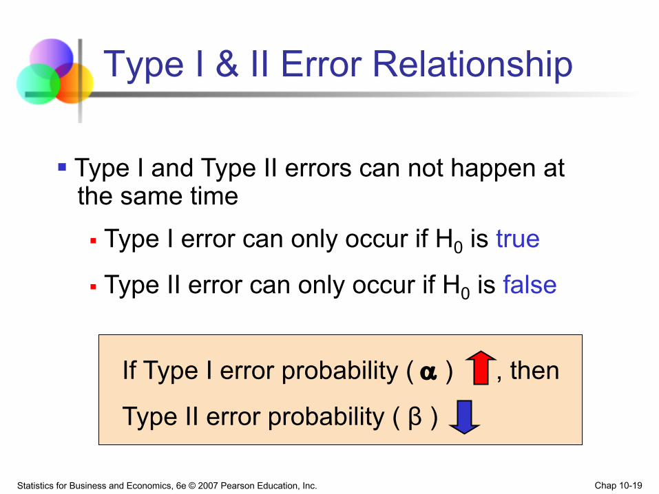
Type I & II Error Relationship

§ Type I and Type II errors can not happen atthe same time§ Type I error can only occur if H0 is true

§ Type II error can only occur if H0 is false

If Type I error probability ( a ) , then

Type II error probability ( β )


Factors Affecting Type II Error

n All else equal,n β when the difference between

hypothesized parameter and its true value

n β when a

n β when σ

n β when n


Power of the Test

n The power of a test is the probability of rejecting a null hypothesis that is false

n i.e., Power = P(Reject H0 | H1 is true)

n Power of the test increases as the sample size increases

Select your test

n Testing is a bit like finding the right recipe based on these ingredients: n Questionn Data typen Sample sizen Variance known? Variance of several groups equal?

n Good news: Plenty of tables available, e.g.,n http://www.ats.ucla.edu/stat/mult_pkg/whatstat/de

fault.htm (with examples in R, SAS, Stata, SPSS)n http://sites.stat.psu.edu/~ajw13/stat500_su_res/not

es/lesson14/images/summary_table.pdf

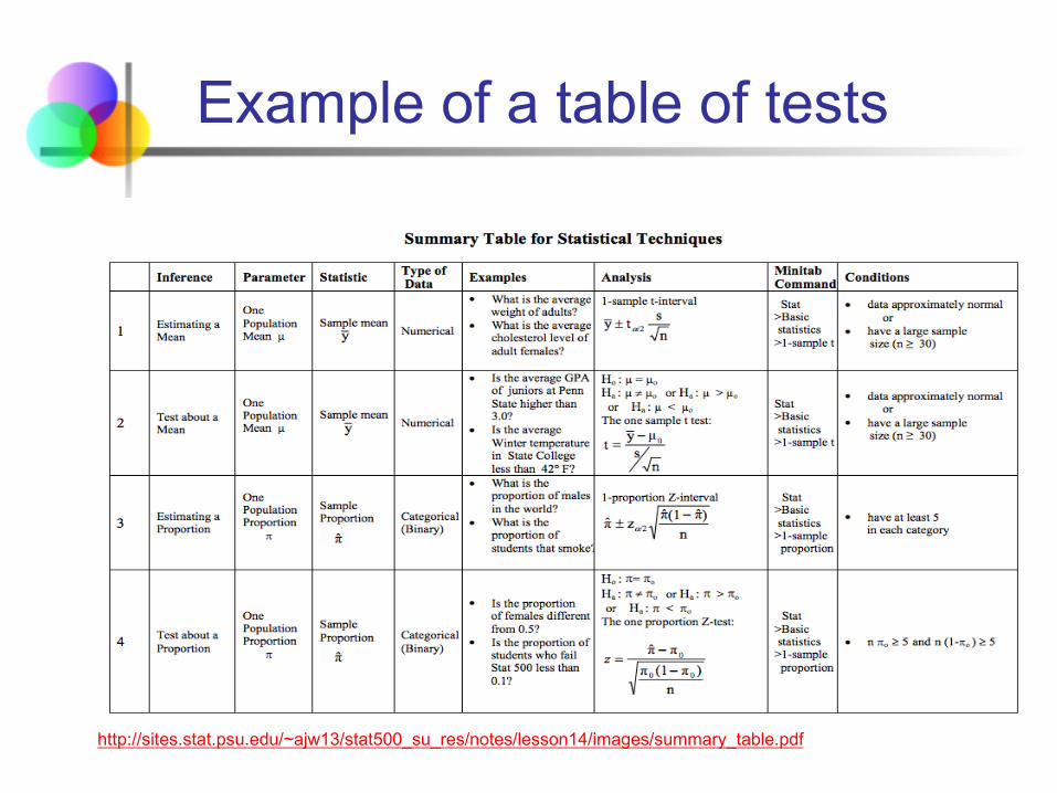
Example of a table of tests

http://sites.stat.psu.edu/~ajw13/stat500_su_res/notes/lesson14/images/summary_table.pdf

A common test: One-sample t-test

n When: Estimating a mean, comparing mean to a hypothetical value

n Requirements: Data approx. normal or sample size > 30

n Setup:

n Evaluation: Compare t-statistic (table, excel) to your value and accept / reject null hypothesis


Hypothesis Tests for the Mean

s Known s Unknown

Hypothesis Tests for µ


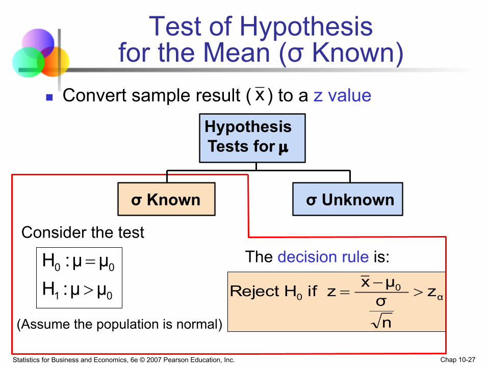
Test of Hypothesisfor the Mean (σ Known)

n Convert sample result ( ) to a z value

The decision rule is:

α0

0 z

nσμxz if H Reject >

-=

σ Known σ Unknown


Consider the test

00 μμ:H =

01 μμ:H >

(Assume the population is normal)

x


Reject H0Do not reject H0

Decision Rule

a

zα0

μ0

H0: μ = μ0

H1: μ > μ0

Critical value

Z

α0

0 z

nσμxz if H Reject >

-=

nσ/ZμX if H Reject α00 +>

nσzμ α0 +

Alternate rule:

x


p-Value Approach to Testing

n p-value: Probability of obtaining a test statistic more extreme ( ≤ or ³ ) than the observed sample value given H0 is true

n Also called observed level of significance

n Smallest value of a for which H0 can be rejected


p-Value Approach to Testing

n Convert sample result (e.g., ) to test statistic (e.g., z statistic )

n Obtain the p-valuen For an upper

tail test:

n Decision rule: compare the p-value to a

n If p-value < a , reject H0

n If p-value ³ a , do not reject H0

(continued)x

)μμ | nσ/μ-x P(Z

true) is H that given , nσ/μ-x P(Z value-p

00

00

=>=

>=


Example: Upper-Tail Z Test for Mean (s Known)

A phone industry manager thinks that customer monthly cell phone bill have increased, and now average over $52 per month. The company wishes to test this claim. (Assume s = 10 is known)

H0: μ ≤ 52 the average is not over $52 per monthH1: μ > 52 the average is greater than $52 per month

(i.e., sufficient evidence exists to support the manager’s claim)

Form hypothesis test:



n Suppose that a = .10 is chosen for this test

Find the rejection region:

a = .10

1.280

Reject H0

Example: Find Rejection Region(continued)

1.28nσ/μxz if H Reject 0

0 >-

=


Obtain sample and compute the test statistic

Suppose a sample is taken with the following results: n = 64, x = 53.1 (s=10 was assumed known)

n Using the sample results,

0.88

6410

5253.1

nσμxz 0 =

-=

-=

Example: Sample Results(continued)



Example: Decision

a = .10

1.280

Reject H0

Do not reject H0 since z = 0.88 < 1.28i.e.: there is not sufficient evidence that the

mean bill is over $52

z = 0.88

Reach a decision and interpret the result:(continued)


Reject H0

a = .10

Do not reject H0 1.280

Reject H0

Z = .88

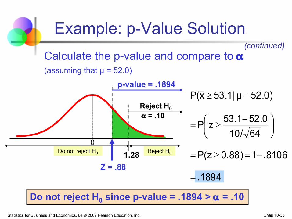
Calculate the p-value and compare to a(assuming that μ = 52.0)

(continued)

.1894

.810610.88)P(z

6410/52.053.1zP

52.0) μ | 53.1xP(

=

-=³=

÷ø

öçè

æ -³=

=³p-value = .1894

Example: p-Value Solution

Do not reject H0 since p-value = .1894 > a = .10


One-Tail Tests

n In many cases, the alternative hypothesis focuses on one particular direction

H0: μ ≥ 3 H1: μ < 3

H0: μ ≤ 3 H1: μ > 3

This is a lower-tail test since the alternative hypothesis is focused on the lower tail below the mean of 3

This is an upper-tail test since the alternative hypothesis is focused on the upper tail above the mean of 3



Upper-Tail Tests

a

zα0μ

H0: μ ≤ 3 H1: μ > 3

n There is only one critical value, since the rejection area is in only one tail

Critical value

Zx


Reject H0 Do not reject H0

n There is only one critical value, since the rejection area is in only one tail

Lower-Tail Tests

a

-za 0

μ

H0: μ ≥ 3 H1: μ < 3

Z

Critical value

x


Do not reject H0 Reject H0Reject H0

n There are two critical values, defining the two regions of rejection

Two-Tail Tests

a/2

0

H0: μ = 3 H1: μ ¹ 3

a/2

Lower critical value

Uppercritical value

3

z

x

-za/2 +za/2

n In some settings, the alternative hypothesis does not specify a unique direction


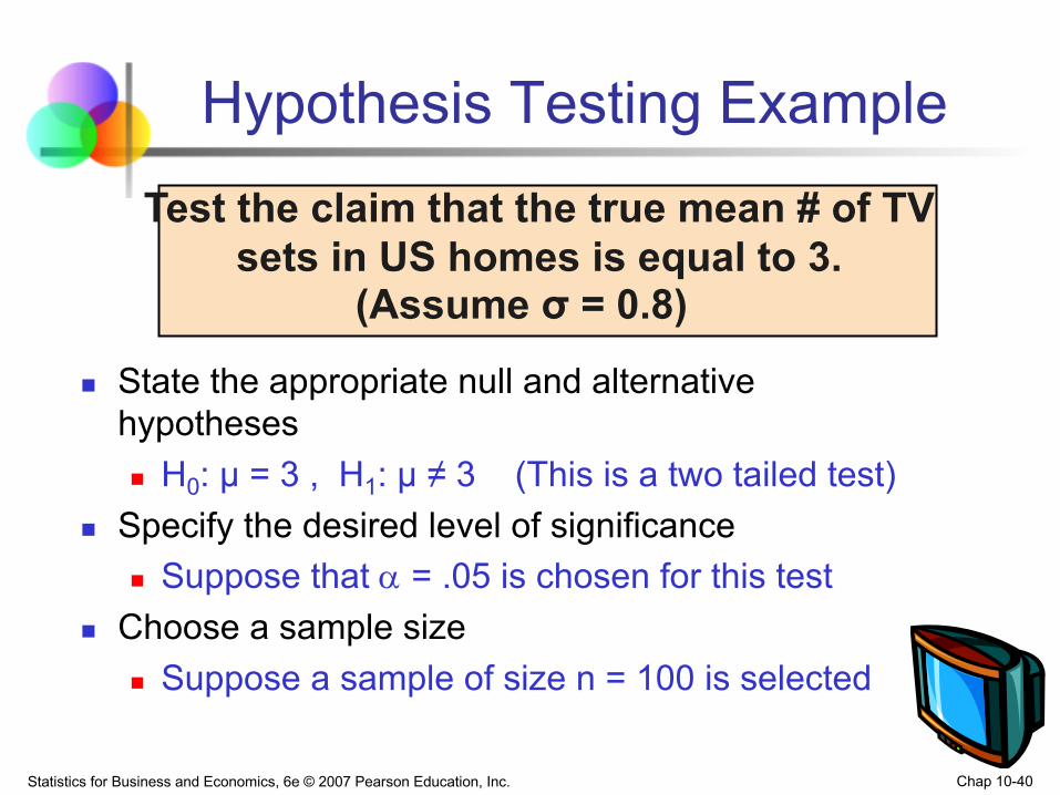
Hypothesis Testing ExampleTest the claim that the true mean # of TV

sets in US homes is equal to 3.(Assume σ = 0.8)

n State the appropriate null and alternativehypothesesn H0: μ = 3 , H1: μ ≠ 3 (This is a two tailed test)

n Specify the desired level of significancen Suppose that a = .05 is chosen for this test

n Choose a sample sizen Suppose a sample of size n = 100 is selected


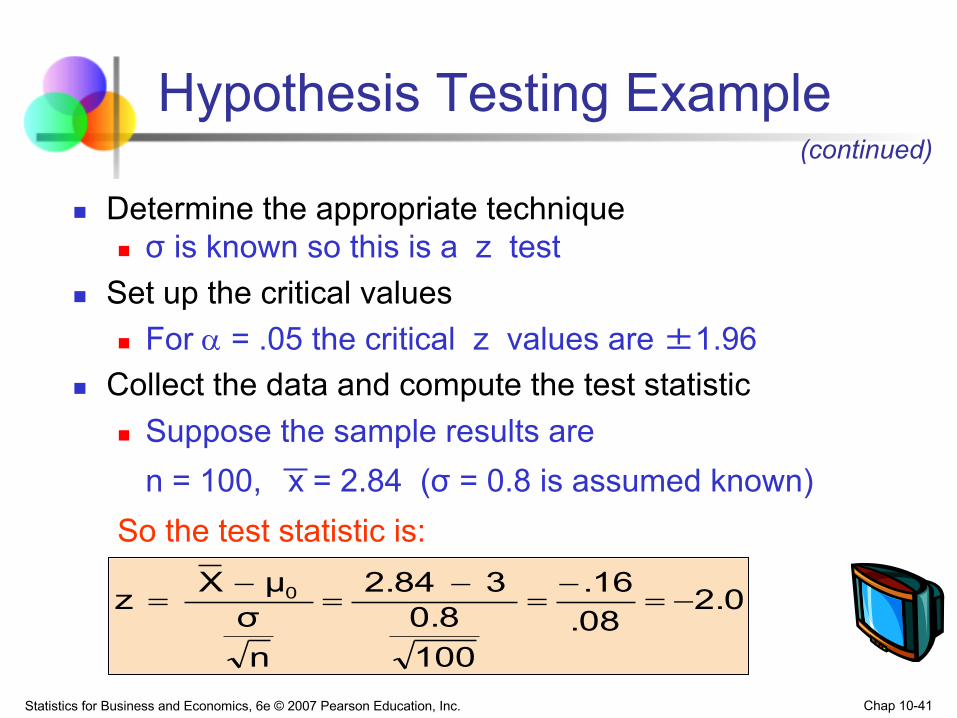
2.0.08.16

1000.8

32.84

nσμXz 0 -=

-=

-=

-=

Hypothesis Testing Example

n Determine the appropriate techniquen σ is known so this is a z test

n Set up the critical valuesn For a = .05 the critical z values are ±1.96

n Collect the data and compute the test statisticn Suppose the sample results are

n = 100, x = 2.84 (σ = 0.8 is assumed known)So the test statistic is:

(continued)



n Is the test statistic in the rejection region?

a = .05/2

-z = -1.96 0

Reject H0 if z < -1.96 or z > 1.96; otherwise do not reject H0

Hypothesis Testing Example(continued)

a = .05/2

Reject H0

+z = +1.96

Here, z = -2.0 < -1.96, so the test statistic is in the rejection region


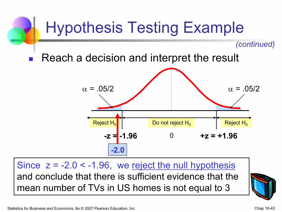
n Reach a decision and interpret the result

-2.0

Since z = -2.0 < -1.96, we reject the null hypothesisand conclude that there is sufficient evidence that the mean number of TVs in US homes is not equal to 3

Hypothesis Testing Example(continued)


a = .05/2

-z = -1.96 0

a = .05/2

Reject H0

+z = +1.96


.0228

a/2 = .025

Example: p-Value

n Example: How likely is it to see a sample mean of 2.84 (or something further from the mean, in either direction) if the true mean is µ = 3.0?

-1.96 0-2.0

.02282.0)P(z

.02282.0)P(z

=>

=-<

Z1.962.0

x = 2.84 is translated to a z score of z = -2.0

p-value

= .0228 + .0228 = .0456

.0228

a/2 = .025


n Compare the p-value with an If p-value < a , reject H0

n If p-value ³ a , do not reject H0

Here: p-value = .0456a = .05

Since .0456 < .05, we reject the null hypothesis

(continued)

Example: p-Value

.0228

a/2 = .025

-1.96 0-2.0

Z1.962.0

.0228

a/2 = .025

AnAlternativeWay

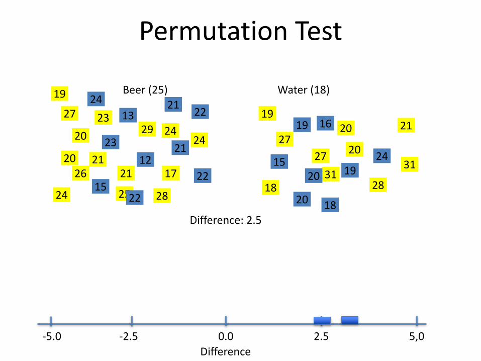
Beer(25):27202126273124212019232428192429182017312025282127Mean:23.6

Water(18):212215122116191522241923132220241820Mean:19.2

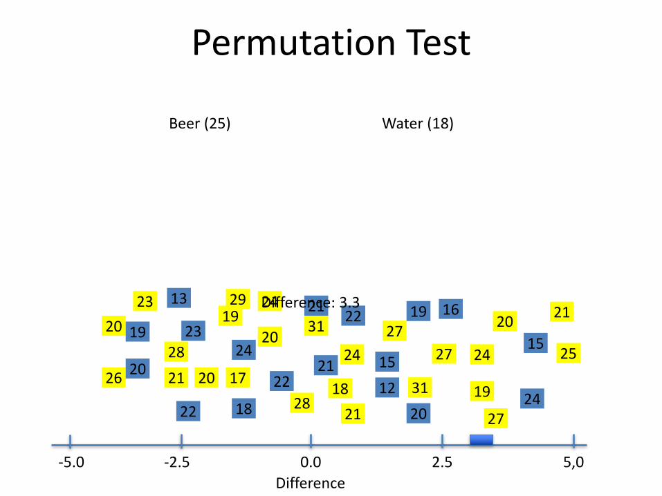
BeerConsumptionIncreasesHumanAttractivenesstoMalariaMosquitoes

BeerConsumption#HumanAttractivenesstoMalariaMosquitoesThierryLefèvre ,Louis-ClémentGouagna,Kounbobr Roch Dabiré,EricElguero,DidierFontenille,FrançoisRenaud,CarloCostantini,Frédéric Thomas

Isadifferenceof4.4significant?

PermutationTest

2720212627

31

24212019

2324281924

29

18201731

2025282127

2122151221

16

19152224

1923132220

24

1820

Beer(25) Water(18)

Difference:4.4

0.0Difference

2.5 5,0-2.5-5.0

PermutationTest

27

2021

2627

31

24

21

2019

23

24

28

192429

18

20

17

3120

252821

27

2122

1512

21 1619

15

22

24

1923

13

22 202418

20

Beer(25) Water(18)

0.0Difference

2.5 5,0-2.5-5.0

PermutationTest

27

2021

2627

31

24

21

2019

23

24

28

192429

18

20

17

3120

252821

27

2122

1512

21 1619

15

22

24

1923

13

22 202418

20

Beer(25) Water(18)

0.0Difference

2.5 5,0-2.5-5.0

Difference:3.3

PermutationTest

Beer(25) Water(18)

0.0Difference

2.5 5,0-2.5-5.0

27

2021

262731

24

2120

19

23

24 28

192429

18

2017

31

20

2528

21

2721

221512

2116

1915

22

24

1923

13

22 20

24

18

20

Difference:2.5

PermutationTest

Beer(25) Water(18)

0.0Difference

2.5 5,0-2.5-5.0

27

2021

262731

24

2120

19

23

24 28

192429

18

2017

31

20

2528

21

2721

221512

2116

1915

22

24

1923

13

22 20

24

18

20

1outof100repetitions


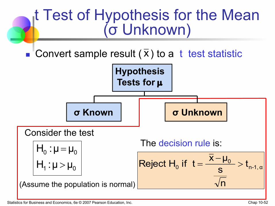
t Test of Hypothesis for the Mean (σ Unknown)

n Convert sample result ( ) to a t test statistic

σ Known σ Unknown


x


α , 1-n0

0 t

nsμxt if H Reject >

-=

Consider the test

00 μμ:H =

01 μμ:H >

(Assume the population is normal)


t Test of Hypothesis for the Mean (σ Unknown)

n For a two-tailed test:


α/2 , 1-n0

α/2 , 1-n0

0 t

nsμxt if or t

nsμxt if H Reject >

-=-<

-=

Consider the test

00 μμ:H =

01 μμ:H ¹

(Assume the population is normal, and the population variance is unknown)

(continued)

What is a T-distribution?

n A t-distribution is like a Z distribution, except has slightly fatter tails to reflect the uncertainty added by estimating s.

n The bigger the sample size (i.e., the bigger the sample size used to estimate s), then the closer t becomes to Z.

n If n>100, t approaches Z.

The T probability density function

Where:v is the degrees of freedom

(gamma) is the Gamma function is the constant Pi (3.14...)

Student’s t Distribution

t0

t (df = 5)

t (df = 13)t-distributions are bell-

shaped and symmetric, but have ‘fatter’ tails than the

normal

Standard Normal

(t with df = ¥)

Note: t Z as n increases

from “Statistics for Managers” Using Microsoft® Excel 4th Edition, Prentice-Hall 2004

Student’s t Table

Upper Tail Area

df .25 .10 .05

1 1.000 3.078 6.314

2 0.817 1.886 2.920

3 0.765 1.638 2.353

t0 2.920The body of the table contains t values, not

probabilities

Let: n = 3 df = n - 1 = 2

a = .10a/2 =.05

a/2 = .05


t distribution values

With comparison to the Z valueConfidence t t t ZLevel (10 d.f.) (20 d.f.) (30 d.f.) ____

.80 1.372 1.325 1.310 1.28

.90 1.812 1.725 1.697 1.64

.95 2.228 2.086 2.042 1.96

.99 3.169 2.845 2.750 2.58

Note: t Z as n increases


Summary: Single population mean (small n, normality)

n Hypothesis test:

n Confidence Intervalnstx

nmean nullmean observed

1-

=-

)(* tmean observed interval confidence /21,-n nsx

a±=

Summary: Single population mean (large n)

n Hypothesis test:

n Confidence IntervalnstZx

nmean nullmean observed

1-

=@ -

)(*]Z t[mean observed interval confidence /2/21,-n nsx

aa @±=


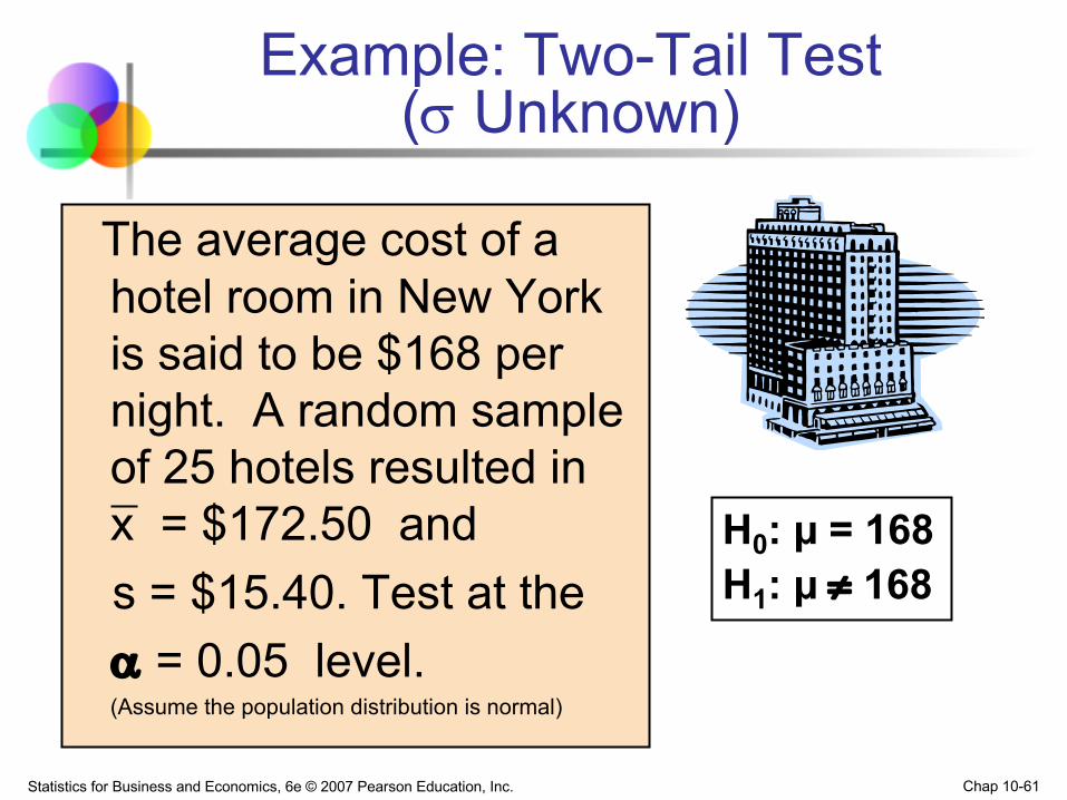
Example: Two-Tail Test(s Unknown)

The average cost of a hotel room in New York is said to be $168 per night. A random sample of 25 hotels resulted in x = $172.50 and s = $15.40. Test at the a = 0.05 level.(Assume the population distribution is normal)

H0: μ = 168 H1: μ ¹ 168


n a = 0.05

n n = 25n s is unknown, so

use a t statisticn Critical Value:

t24 , .025 = ± 2.0639

Example Solution: Two-Tail Test

Do not reject H0: not sufficient evidence that true mean cost is different than $168

Reject H0Reject H0

a/2=.025

-t n-1,α/2Do not reject H0

0

a/2=.025

-2.0639 2.0639

1.46

2515.40

168172.50

nsμxt 1n =

-=

-=-

1.46

H0: μ = 168 H1: μ ¹ 168

t n-1,α/2


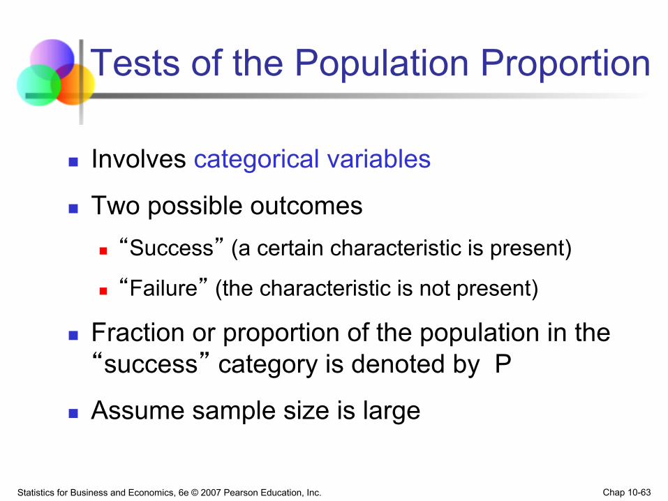
Tests of the Population Proportion

n Involves categorical variables

n Two possible outcomesn “Success” (a certain characteristic is present)

n “Failure” (the characteristic is not present)

n Fraction or proportion of the population in the “success” category is denoted by P

n Assume sample size is large


Proportions

n Sample proportion in the success category is denoted by

n

n When nP(1 – P) > 9, can be approximated by a normal distribution with mean and standard deviationn

sizesamplesampleinsuccessesofnumber

nxp ==ˆ

Pμ =p̂nP)P(1σ -

=p̂

(continued)

p̂

p̂


n The sampling distribution of is approximately normal, so the test statistic is a z value:

Hypothesis Tests for Proportions

n)P(1P

Ppz00

0

--

=ˆ

nP(1 – P) > 9

Hypothesis Tests for P

Exact test

p̂

nP(1 – P) < 9


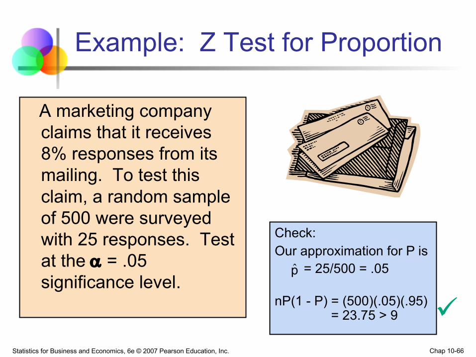
Example: Z Test for Proportion

A marketing company claims that it receives 8% responses from its mailing. To test this claim, a random sample of 500 were surveyed with 25 responses. Test at the a = .05 significance level.

Check: Our approximation for P is

= 25/500 = .05

nP(1 - P) = (500)(.05)(.95)= 23.75 > 9

p̂

ü


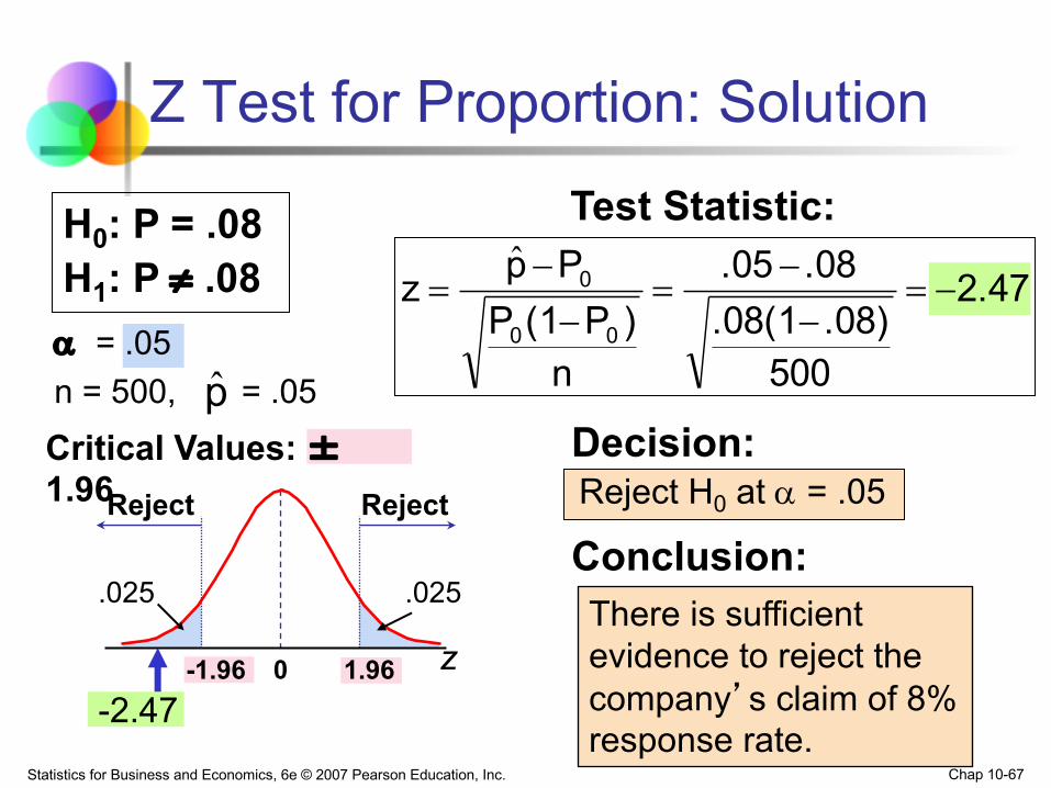
Z Test for Proportion: Solution

a = .05 n = 500, = .05

Reject H0 at a = .05

H0: P = .08 H1: P ¹ .08

Critical Values: ±1.96

Test Statistic:

Decision:

Conclusion:

z0

Reject Reject

.025.025

1.96-2.47

There is sufficient evidence to reject the company’s claim of 8% response rate.

2.47

500.08).08(1.08.05

n)P(1P

Ppz00

0 -=--

=-

-=

ˆ

-1.96

p̂


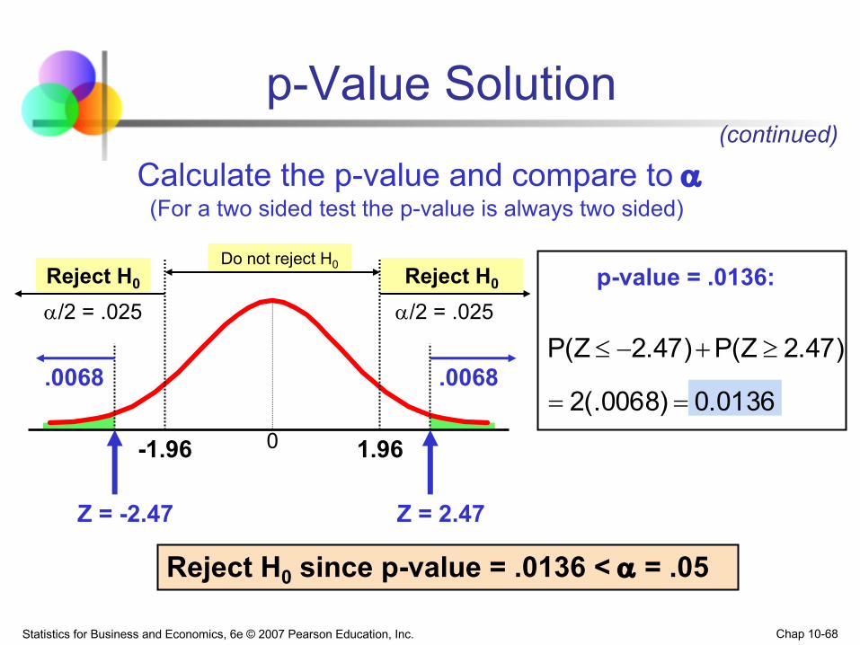
Do not reject H0 Reject H0Reject H0

a/2 = .025

1.960

Z = -2.47

Calculate the p-value and compare to a(For a two sided test the p-value is always two sided)

(continued)

0.01362(.0068)

2.47)P(Z2.47)P(Z

==

³+-£

p-value = .0136:

p-Value Solution

Reject H0 since p-value = .0136 < a = .05

Z = 2.47

-1.96

a/2 = .025

.0068.0068


n Recall the possible hypothesis test outcomes:Actual Situation

Decision

Do Not Reject H0

No error(1 - )a

Type II Error( β )

Reject H0Type I Error

( )a

H0 FalseH0 TrueKey:

Outcome(Probability)

No Error( 1 - β )

n β denotes the probability of Type II Error n 1 – β is defined as the power of the test

Power = 1 – β = the probability that a false null hypothesis is rejected

Power of the Test


Type II Error

or


α0

0 zn/σμxz if H Reject >

-=

00 μμ:H =

01 μμ:H >

Assume the population is normal and the population variance is known. Consider the test

nσ/Zμxx if H Reject α0c0 +>=

If the null hypothesis is false and the true mean is μ*, then the probability of type II error is

÷÷ø

öççè

æ -<==<=

n/σ*μxzPμ*)μ|xxP(β c

c


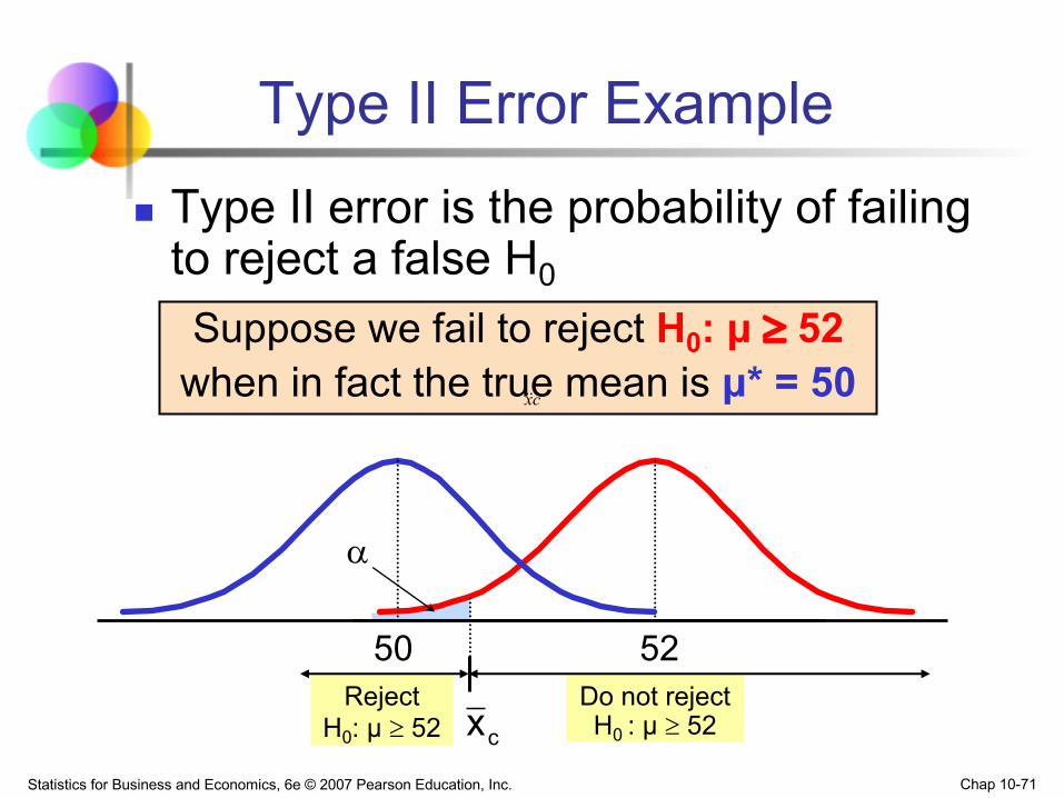
Reject H0: μ ³ 52

Do not reject H0 : μ ³ 52

Type II Error Examplen Type II error is the probability of failing

to reject a false H0

5250

Suppose we fail to reject H0: μ ³ 52when in fact the true mean is μ* = 50

a

cx!!

cx


Reject H0: μ ³ 52


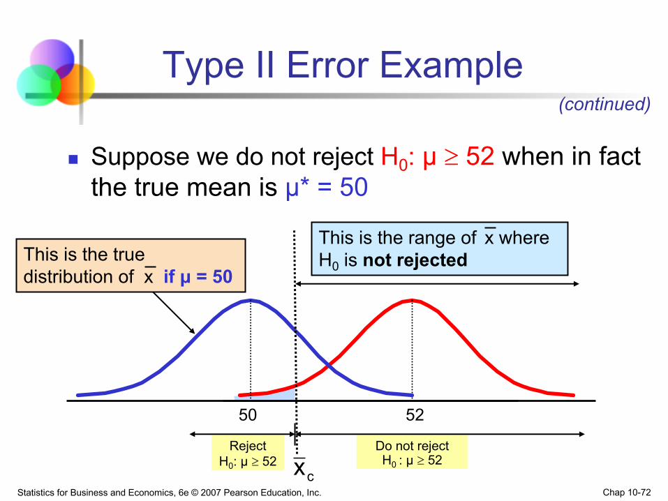
Type II Error Example

n Suppose we do not reject H0: μ ³ 52 when in fact the true mean is μ* = 50

5250

This is the true distribution of x if μ = 50

This is the range of x where H0 is not rejected

(continued)

cx


Reject H0: μ ³ 52


Type II Error Example

n Suppose we do not reject H0: μ ³ 52 when in fact the true mean is μ* = 50

a

5250

β

Here, β = P( x ³ ) if μ* = 50

(continued)

cx

cx


Reject H0: μ ³ 52


n Suppose n = 64 , σ = 6 , and a = .05

a

5250

So β = P( x ³ 50.766 ) if μ* = 50

Calculating β

50.7666461.64552

nσzμx α0c =-=-=

(for H0 : μ ³ 52)

50.766

cx


Reject H0: μ ³ 52


.1539.3461.51.02)P(z64

65050.766zP50)μ*|50.766xP( =-=³=

÷÷÷

ø

ö

ççç

è

æ-

³==³

n Suppose n = 64 , σ = 6 , and a = .05

a

5250

Calculating β(continued)

Probability of type II error:

β = .1539

cx


If the true mean is μ* = 50,n The probability of Type II Error = β = 0.1539n The power of the test = 1 – β = 1 – 0.1539 = 0.8461

Power of the Test Example

Actual SituationDecision

Do Not Reject H0

No error1 - a = 0.95

Type II Errorβ = 0.1539

Reject H0Type I Errora = 0.05

H0 FalseH0 TrueKey:

Outcome(Probability)

No Error1 - β = 0.8461

(The value of β and the power will be different for each μ*)

hypothesis testing - brown university · 11.3 research hypothesis testing… the fda or...

Documents