hyperpolarization -description, overview & method · para-hydrogen induced polarization (phip)...

Hyperpolarization - Description, Overview & MethodEducational Session, ISMRM 2017

April 26, 2017

Peder Larson, Ph.D.Associate Professor, Department of Radiology and Biomedical Imaging, University of California, San Francisco, CA, United States

[email protected]://radiology.ucsf.edu/research/labs/larson@pezlarson

Speaker Name: Peder Larson

I have the following financial interest or relationship to disclose with regard to the subject matter of this presentation:

Company Name: GE HealthcareType of Relationship: Research Support

Declaration ofFinancial Interests or Relationships

Outline

https://radiology.ucsf.edu/research/labs/larson/educational-materials

(Google: Peder Larson Lab, Educational Materials link on sidebar)

§ Hyperpolarization

• What does it mean?

• Dissolution Dynamic Nuclear Polarization (dDNP)

• Spin Exchange Optical pumping

• Para-hydrogen induced polarization (PHIP, SABRE)

§ Imaging Methods

• RF pulse strategies

• Acquisition strategies

• Analysis – kinetic models

April 26, 2017Hyperpolarization Methods3

Spin Polarization

4

Spins

µ

B = 0

µ

µ

µ

µ

M0 = 0

Net Magnetization

netic field, it will be found to be either in the spin-upor spin-down state, no matter which mixed state cj iit was in before. Furthermore, it will stay in that newstate until the proton is subject to more interactionswith environment (e.g. another measurement). Thisso-called collapse into an eigenstate is a consequenceof QM. It apparently implies that a measurement ofthe net magnetization (e.g. by MRI), will force eachproton into either the spin-up or the spin-down statein agreement with myth 1. This is wrong, however.The emphasized word individual above is importantin the present context, as we can only infer from QMthat the protons are forced into single-spin eigen-states, if we measure their magnetization one-by-oneas can be done with a Stern-Gerlach apparatus, forexample (11). In contrast, that is never done in MRspectrometers or scanners: to get a measurable MR-signal the total magnetization of many nuclei isalways measured, and myth 1 does not follow. Itcould be true nevertheless, but in fact it is not, whichis shown in appendix (proposition 1) by employingthe QM formalism: A measurement of the net mag-netization causes a perturbation of the system that isinsufficient to affect the individual protons signifi-cantly. In particular, they are not brought into theireigenstates by the measurement process.

It is worth noting that even though the argumentsmentioned above may occur complicated for the non-technical reader, they are what many students of MRmore or less implicitly lay ears to, and for no goodreason, as QM is not needed for understanding basicMR. Moreover, the students often hear the wrongversion of the argument.

The lifetime of myth 1 may have been prolongedby an observation that many working with MR have

made: when subject to a magnetic field, an oblong pi-ece of magnetizable material have a strong tendencyto align itself in one of two opposite directions paral-lel to the field (in contrast to permanently magnetizedmaterial that orient itself in one direction only). De-spite a superficial resemblance, this well-known phe-nomenon has nothing to do with the effect expressedin myth 1. Rather it is a consequence of reorientationof magnetic constituents inside the metal. This givesrise to the existence of two low-energy states for theorientation of the metallic piece, parallel and antipar-allel to the field. The magnetic constituents are in ei-ther case parallel to the field, because they have onlyone low-energy state. Similarly, the proton spin hasonly one low-energy state. Nothing but MR-irrele-vant single-proton measurements give spins a tend-ency to align antiparallel to the field.

Consequently, spins can point in any direction andthe energy eigenstates are not more relevant to MRthan any other state (the eigenstates form a conven-ient basis for computations, but they are irrelevantfor the understanding). Hence Fig. 1 that illustratesthe nature of spin eigenstates, do not contribute muchbut confusion in an MR context. QM is later shownto imply that the spin-evolution of individual protonshappens as expected classically unless perturbed,e.g., by a single-spin measurement.

Finally, replacements for Fig. 1 are discussed.According to both classical and QM, spins areexpected to point in all directions in the absence offield as shown in Fig. 2. Except for precession, thesituation does not change much when the polarizingB0-field used for MR is applied as shown in Fig. 3.The energies associated with the orientation of theindividual spins are much smaller than the thermal

Figure 2 In the absence of magnetic field, the spins are pointing randomly hence giving aspherical distribution of spin orientations. This is illustrated to the right by a large number ofexample spins in an implicit magnetization coordinate space similar to that of Fig. 1. [Color fig-ure can be viewed in the online issue, which is available at www.interscience.wiley.com.]

332 HANSON

Concepts in Magnetic Resonance Part A (Bridging Education and Research) DOI 10.1002/cmr.a

Danish Research Centre for Magnetic Resonance. Educational Materials: http://www.drcmr.dk/educations/education-material

April 26, 2017Hyperpolarization Methods

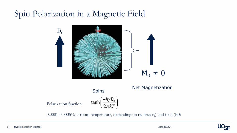
Spin Polarization in a Magnetic Field

5

Spins

µB0µ

µ

µ

µ

M0 ≠ 0

Net Magnetization

energies so the spins only have a slight tendency topoint along the direction of the field (and noincreased tendency to point opposite the field, neitherclassically, nor quantum mechanically). The situationcan be compared to the one described earlier involv-ing a hypothetical collection of compasses placed inthe earth magnetic field. All compasses will swing tothe north, if they are noninteracting and not dis-turbed. The situation changes if the compasses areplaced in a running tumble-dryer or similar deviceincreasing the collisional energies above those asso-ciated with changing the direction of the compassneedles. The bouncing and interacting compasseswill no longer all point toward north but there willstill be a slight tendency for them to do so. If the netmagnetization is measured, it will point toward north.The situation is like that of the moving protons in aliquid sample where the magnetic interactionsbetween neighboring nuclei cause reorientation ofthe magnetic moments (relaxation). In the absence ofa magnetic field, the angular distribution of spins isspherical in either case. When a field is added, thedistribution is skewed slightly toward the field direc-tion by relaxation.

It is important to understand that precession of theindividual nuclei starts as soon as the sample isplaced in the field (not only after excitation by RFfields, as frequently stated). The nuclei therefore emitradio waves at the Larmor frequency as soon as theyare placed in the field. Similarly, however, theyabsorb radio waves emitted by their neighbors andsurroundings. Because the distribution of spin direc-tions is even in the transversal plane, the net trans-versal magnetization is zero, and there is no netexchange of energy between the sample and its sur-roundings. The exchange of radio waves within thesample is nothing but magnetic interactions betweenneighboring nuclei. These are responsible forrelaxation.

Myth 2: MR Is a Quantum Effect

A quantum effect is a phenomenon that cannot beadequately described by classical mechanics, i.e., onewhere only QM give predictions in accordance withobservations. In the introduction, it was stated thatatom formation is a quantum effect because atomsare not expected to be stable according to classicalmechanics, whereas experiments have proven thatthey are. This does not imply that all phenomenainvolving atoms are defined as quantum effects, sincesuch a broad definition would be quite useless.Instead, phenomena are hierarchically divided intoclassical and quantum phenomena, so a classical phe-nomenon can involve atoms that are themselves inex-plicable by classical mechanics. Similarly, protonspin is a quantum effect but MR is not since the latteris accurately described by classical mechanics. Thisis the subject of the present section.

It is often and correctly said that spin is a quantumeffect. From a classical perspective it cannot beexplained why protons apparently all rotate with thesame constant angular frequency, which result in anobservable angular momentum (spin) and associatedmagnetic moment. Despite the fact that this is reallymind-boggling, it is usually not perceived so bystudents of MR. Just as atoms are taken for granted,it is typically accepted without argument that protonsappear to be rotating and that they as a result behaveas small magnets with a north and a south pole, i.e.they have angular and magnetic moments. Mostbooks state this correctly and there is no apparentreason to elaborate, as a deeper understanding of spinis typically of little use in the context of MR.

Even though spin is a quantum effect, MR is not,according to the definition given earlier, as it doesnot necessitate a quantum explanation. Classically, amagnetic dipole M with an associated angular mo-

Figure 3 Better alternative to Fig. 1 showing the spindistribution in a magnetic field. The spins will precess asindicated by the circular arrow and a longitudinal equilib-rium magnetization (large vertical arrow) will graduallyform as the distribution is skewed slightly toward mag-netic north by T1-relaxation (uneven density of arrows).The equilibrium magnetization is stationary, so eventhough the individual spins are precessing, there is no netemission of radio waves in equilibrium. [Color figure canbe viewed in the online issue, which is available atwww.interscience.wiley.com.]

UNDERSTANDING MAGNETIC RESONANCE 333

Concepts in Magnetic Resonance Part A (Bridging Education and Research) DOI 10.1002/cmr.a

Polarization fraction:

0.0001-0.0005% at room temperature, depending on nucleus (γ) and field (B0)

tanh −hγB02πkT

"

#$

%

&'


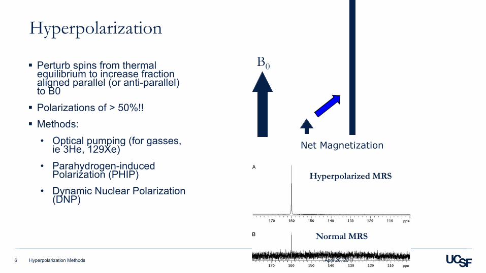
Hyperpolarization

§ Perturb spins from thermal equilibrium to increase fraction aligned parallel (or anti-parallel) to B0

§ Polarizations of > 50%!!§ Methods:

• Optical pumping (for gasses, ie 3He, 129Xe)

• Parahydrogen-induced Polarization (PHIP)

• Dynamic Nuclear Polarization (DNP)

6

Hyperpolarized MRS

Normal MRS

B0

Net Magnetization


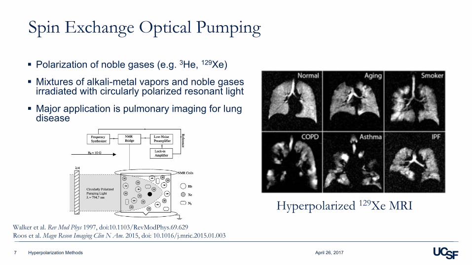
Spin Exchange Optical Pumping

§ Polarization of noble gases (e.g. 3He, 129Xe)

§ Mixtures of alkali-metal vapors and noble gases irradiated with circularly polarized resonant light

§ Major application is pulmonary imaging for lung disease


Hyperpolarized 129Xe MRI Walker et al. Rev Mod Phys 1997, doi:10.1103/RevModPhys.69.629Roos et al. Magn Reson Imaging Clin N Am. 2015, doi: 10.1016/j.mric.2015.01.003

Para-hydrogen Induced Polarization (PHIP)

§ Parahydrogen is the Singlet State of Hydrogen gas, H2

§ MR invisible, can store magnetization

§ Transfer the polarization from the singlet-state to other nuclei


Triplets, T+, T0, T-

Singlet, S0

para hydrogen

1H

1Hparahydrogen

1H

Ir

hyperpolarizedsubstrate 1H

reversibleexchange

reversibleexchange

1H1H

J

J SABREAdams, … , Duckett et al.Science 2009 323, 1708

Content Courtesy Thomas Theis

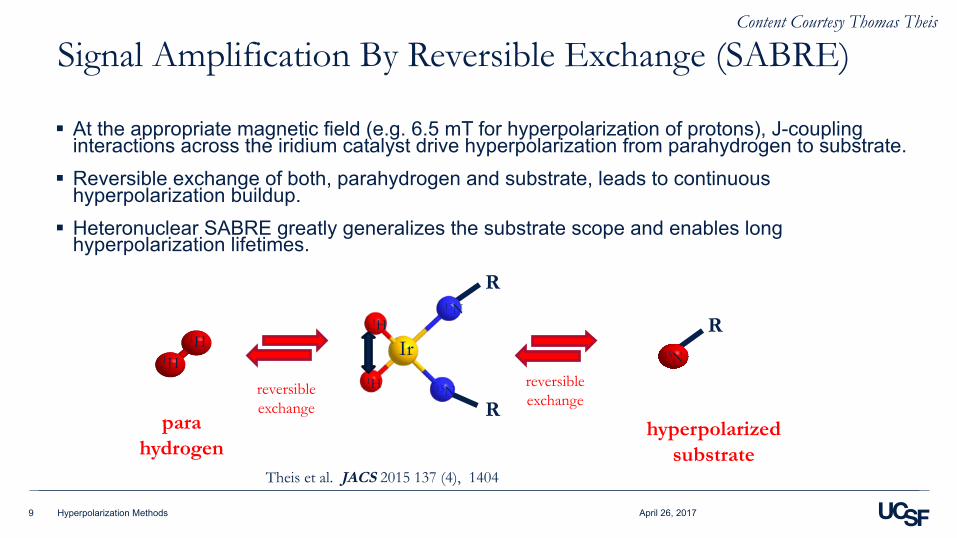
Signal Amplification By Reversible Exchange (SABRE)

§ At the appropriate magnetic field (e.g. 6.5 mT for hyperpolarization of protons), J-coupling interactions across the iridium catalyst drive hyperpolarization from parahydrogen to substrate.

§ Reversible exchange of both, parahydrogen and substrate, leads to continuous hyperpolarization buildup.

§ Heteronuclear SABRE greatly generalizes the substrate scope and enables long hyperpolarization lifetimes.


R1H

1H 15N

Ir

15N

parahydrogen

hyperpolarizedsubstrate

reversibleexchange

reversibleexchange

1H1H

15N

R

R

Theis et al. JACS 2015 137 (4), 1404


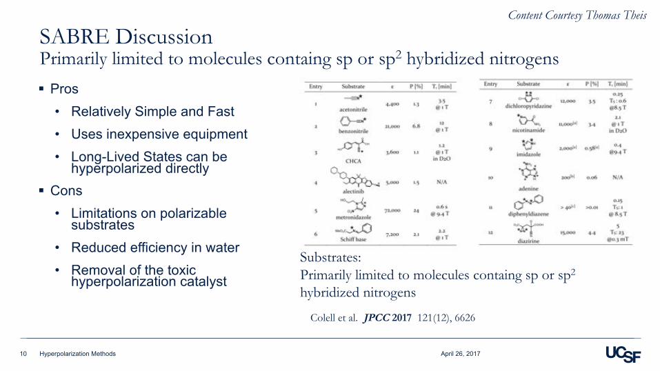
SABRE DiscussionPrimarily limited to molecules containg sp or sp2 hybridized nitrogens§ Pros

• Relatively Simple and Fast• Uses inexpensive equipment• Long-Lived States can be

hyperpolarized directly§ Cons

• Limitations on polarizable substrates

• Reduced efficiency in water• Removal of the toxic

hyperpolarization catalyst

Colell et al. JPCC 2017 121(12), 6626

Substrates:Primarily limited to molecules containg sp or sp2

hybridized nitrogens



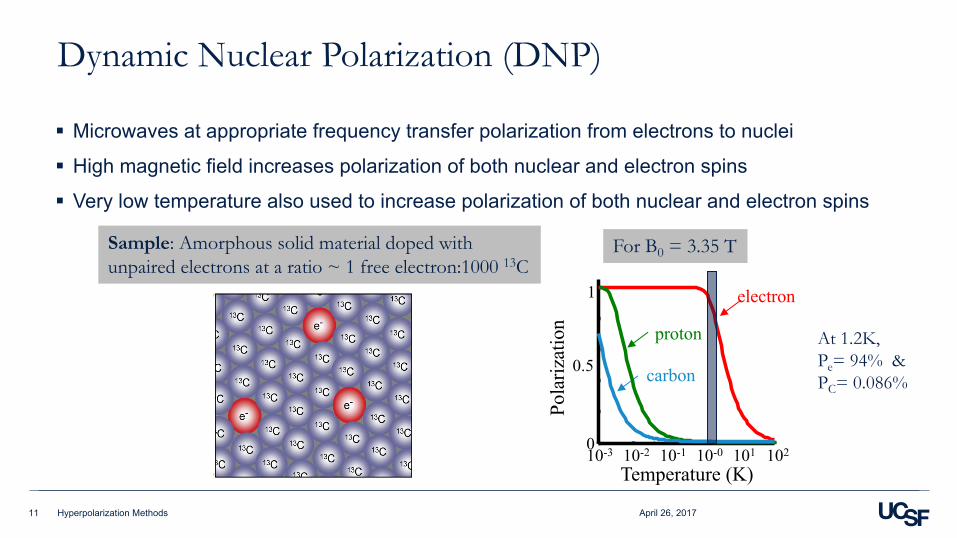
Dynamic Nuclear Polarization (DNP)

§ Microwaves at appropriate frequency transfer polarization from electrons to nuclei

§ High magnetic field increases polarization of both nuclear and electron spins

§ Very low temperature also used to increase polarization of both nuclear and electron spins

11

Temperature (K)

Pola

rizat

ion proton

carbon

10-30

0.5

1 electron

10-2 10-1 10-0 101 102

At 1.2K, Pe= 94% & PC= 0.086%

For B0 = 3.35 TSample: Amorphous solid material doped with unpaired electrons at a ratio ~ 1 free electron:1000 13C


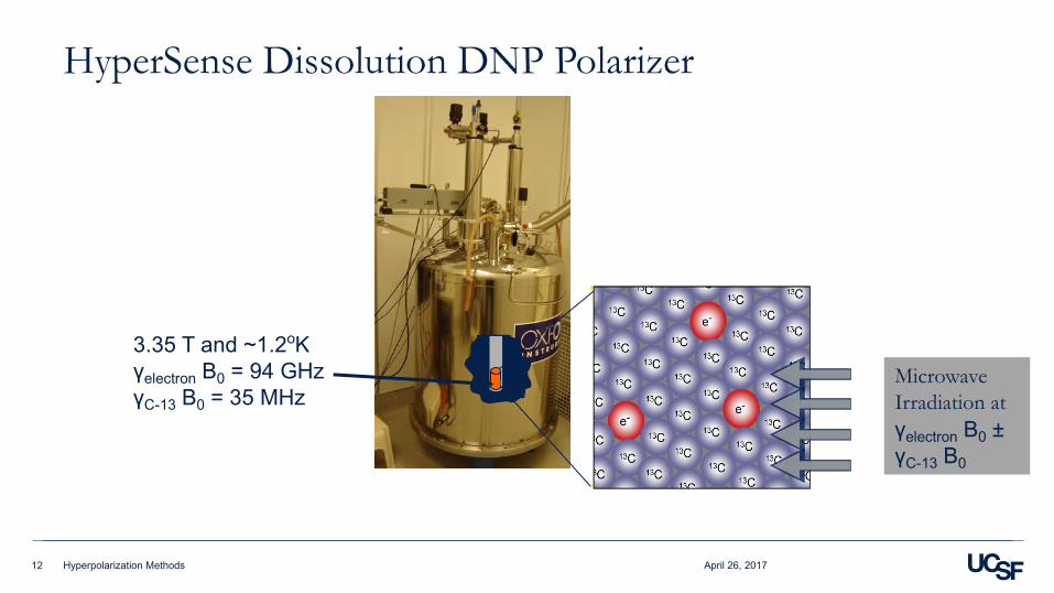
3.35 T and ~1.2oKγelectron B0 = 94 GHzγC-13 B0 = 35 MHz

HyperSense Dissolution DNP Polarizer

12

Microwave Irradiation atγelectron B0 ±γC-13 B0


• The buffer is heated and pressurized

• The sample space is pressurized

• The sample is raised out of the liquid helium

• The dissolution stick is lowered, docking with the sample holder

• The solvent is injected, dissolving the sample, while preserving the enhanced polarization

Slide courtesy of Jan Henrik Ardenkjaer-Larsen, GE Healthcare

Dissolution DNP Procedure

13 April 26, 2017Hyperpolarization Methods

SpinLab Clinical Polarizer

12 3 4

SpinLabPolarizer

Ardenkjaer-Larsen et al. NMR Biomed 2011; 24:927

5 T and ~0.8oKγelectron B0 = 140 GHzγC-13 B0 = 52 MHz

Automated Quality Control System


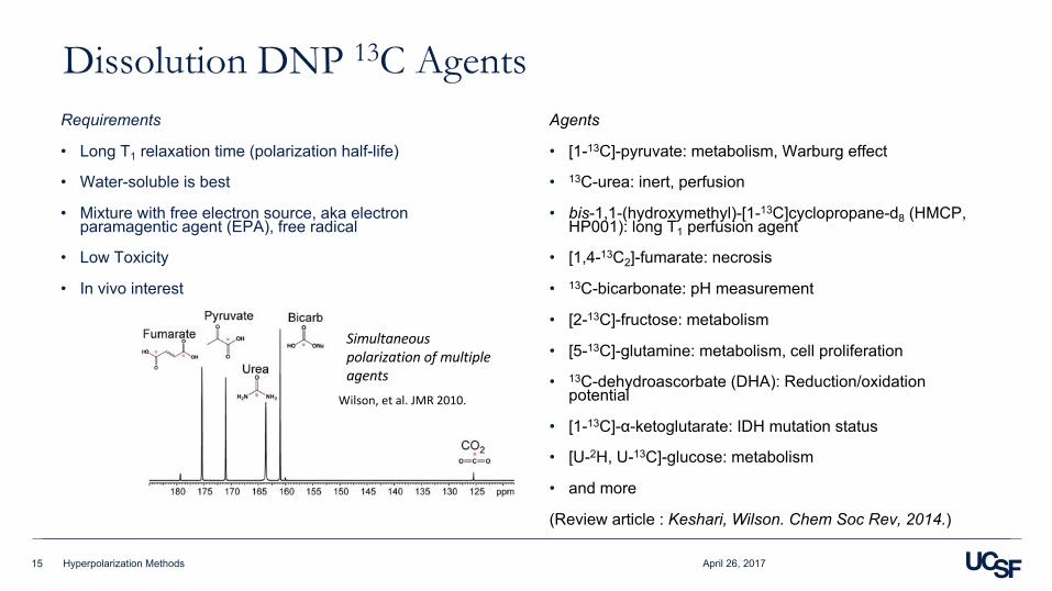
Dissolution DNP 13C AgentsRequirements

• Long T1 relaxation time (polarization half-life)

• Water-soluble is best

• Mixture with free electron source, aka electron paramagentic agent (EPA), free radical

• Low Toxicity

• In vivo interest

Agents

• [1-13C]-pyruvate: metabolism, Warburg effect

• 13C-urea: inert, perfusion

• bis-1,1-(hydroxymethyl)-[1-13C]cyclopropane-d8 (HMCP, HP001): long T1 perfusion agent

• [1,4-13C2]-fumarate: necrosis

• 13C-bicarbonate: pH measurement

• [2-13C]-fructose: metabolism

• [5-13C]-glutamine: metabolism, cell proliferation

• 13C-dehydroascorbate (DHA): Reduction/oxidation potential

• [1-13C]-α-ketoglutarate: IDH mutation status

• [U-2H, U-13C]-glucose: metabolism

• and more

(Review article : Keshari, Wilson. Chem Soc Rev, 2014.)

Wilson,etal.JMR2010.

Simultaneouspolarizationofmultipleagents


MGVander Heiden etal.Science2009;324:1029-1033


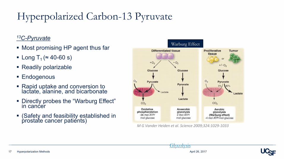
Hyperpolarized Carbon-13 Pyruvate

13C-Pyruvate § Most promising HP agent thus far§ Long T1 (≈ 40-60 s)§ Readily polarizable§ Endogenous§ Rapid uptake and conversion to

lactate, alanine, and bicarbonate§ Directly probes the “Warburg Effect”

in cancer§ (Safety and feasibility established in

prostate cancer patients)

17

Warburg Effect

MGVander Heiden etal.Science2009;324:1029-1033

GlycolysisApril 26, 2017Hyperpolarization Methods

Bloch Equation

18

ddtM =

M ×γ

B+

−1/T2 0 00 −1/T2 00 0 −1/T1

#

$

%%%%

&

'

((((

M +

00

M0 /T1

#

$

%%%

&

'

(((

Net magnetization behavior, hyperpolarized or at thermal equilibrium, is described by Bloch equation:

PrecessionRF Excitation

Relaxation back to thermal equilibrium:

M =

00M0

!

"

###

$

%

&&&


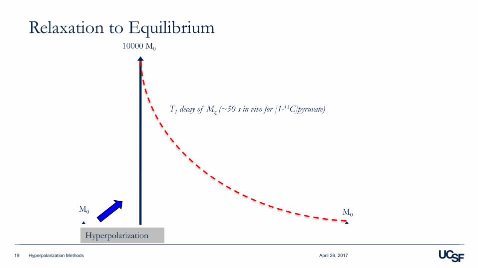
Relaxation to Equilibrium

19

T1 decay of Mz (~50 s in vivo for [1-13C]pyruvate)

Hyperpolarization

M0

10000 M0

M0


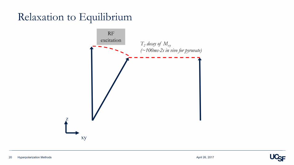
Relaxation to Equilibrium

20

T2 decay of Mxy(~100ms-2s in vivo for pyruvate)

RF excitation

xy

z


13C MR of Pyruvate Metabolism

21

Dynamic MR Spectrum in vivo

frequency

Pyruvate

13C

Lactate

13C

Bicarbonate

13C

Pyruvate-hydrate

Following injection of 13C-pyruvate

Alanine

13C


Hyperpolarized 13C Imaging Procedure

1. Hyperpolarization of 13C-pyruvate (45-90 mins)

2. Rapidly dissolution of frozen compound to create a hyperpolarized liquid agent (10 sec)3. Agent is injected to the subject inside the MRI scanner (10 sec)4. 13C MRI/MRSI is performed immediately (1-2 mins)

22

1,2 3

4


MR Pulse Sequence Components

1. Excite spins (RF)

2. Readout signal (spectral and/or spatial encoding)

3. Repeat

23

Magnetization Vector

MZ

MXYSignal

RF

DAQ

T2

T1

1.

1.

2.

2.

x NTR

3.

T2

T1


Hyperpolarized RF Pulses

Two key considerations:

1. Efficient use of hyperpolarization

• Variable flip angles

• “Multiband” excitation

2. Spectral selectivity

• Spectral-spatial RF pulses

April 26, 201724 Hyperpolarization Methods

Constant Flip Angle

§ Received signal varies between excitations (can cause blurring)§ Residual unused hyperpolarization after last excitation

April 26, 201725

S1 S2 S3 S4 S5 S6

θθ

θθ θ θ

MZ

MXY

Hyperpolarization Methods

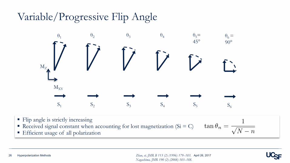
Variable/Progressive Flip Angle

§ Flip angle is strictly increasing§ Received signal constant when accounting for lost magnetization (Si = C)§ Efficient usage of all polarization

April 26, 201726 Zhao, et, JMR B 113 (2) (1996) 179–183.Nagashima, JMR 190 (2) (2008) 183–188.

θ1

S1

θ2 θ3

S2 S3

θ4

S4

θ5= 45°

S5

θ6 = 90°

S6

MZ

MXY


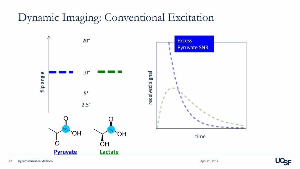
Dynamic Imaging: Conventional Excitation

April 26, 201727

Lactate

13C1

Pyruvate

13C1

flipangle

2.5°

5°

10°

20°

time

received

signal

ExcessPyruvateSNR


Dynamic Imaging: Multiband Excitation

April 26, 201728

flipangle

2.5°

5°

10°

20°

time

received

signal

MorelactateSNRformoretime

PyruvateSNRisstillsufficient

Smallerpyruvateflipleavesmoremagnetizationthatcanthenbecomelactate

Lactate

13C1

Pyruvate

13C1


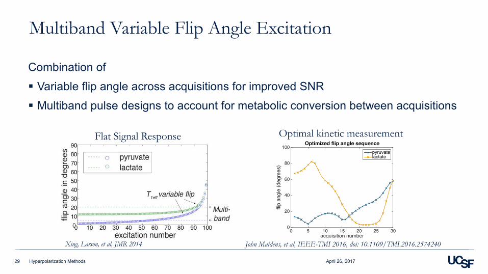
Multiband Variable Flip Angle Excitation

Combination of§ Variable flip angle across acquisitions for improved SNR§ Multiband pulse designs to account for metabolic conversion between acquisitions

April 26, 201729

MANUSCRIPT SUBMITTED TO IEEE TRANSACTIONS ON MEDICAL IMAGING 5

acquisition number0 5 10 15 20 25 30

flip

angl

e (d

egre

es)

0

20

40

60

80

100Optimized flip angle sequence

pyruvatelactate

Fig. 3. Optimized flip angle sequence for estimating the metabolic rateparameter kPL using the nominal parameter values in Table I and a samplinginterval TR = 2 s between acquisitions.

time (s)0 10 20 30 40 50 60

x t (au)

�104

0

0.5

1

1.5

2

2.5Simulated state trajectories

pyruvate (x1t)lactate (x2t)

(a) states xt

time (s)0 10 20 30 40 50 60

Yt (a

u)0

1000

2000

3000

4000

5000

6000

7000Simulated measurement trajectories

pyruvate (Y1t)lactate (Y2t)

(b) Rician-distributed measurementsYt

Fig. 4. Simulated trajectories of the model (2) using the optimized flip anglesequence shown in Fig. 3 and the arterial input function shown in Fig. 2a.

We see that the pyruvate flip angles follow a pattern similarto flip angle sequences designed for other objectives, beginningwith small flip angles to preserve magnetization for futureacquisitions but increasing toward the end of the sequence [9],[10]. In contrast, the optimized flip angle sequence is muchmore aggressive with the lactate flip angles at the beginningof the experiment than in other variable flip angle sequences.This provides more reliable information about the leading endof the lactate time series, which contains the most informationabout the metabolic rate.

For the particular model and regularization parameter valuesused, the BFGS optimization algorithm converges to thesame optimal sequence for a wide range of initializations. Toconfirm this, we have initialized the search algorithm usingthree flip angle sequences with angles generated randomlybetween 0 and 90�. For all three initializations, the algorithmconverges to the flip angle sequence shown in Fig. 3. Thisdemonstrates that the flip angle sequence presented is likely aglobal optimum.

IV. VALIDATION USING SIMULATED DATA

In this section, we demonstrate the advantage of the opti-mally designed flip angle sequence using computer-simulateddata. Working with simulated data allows us to collect a largenumber of statistically independent data sets and provides usaccess to a “ground truth” value for the parameter vector.This makes it possible to reliably determine the parameter

estimation error that results from noise in the simulatedmeasurements. It is not feasible to acquire such a large numberof data sets in vivo, and these would also not include groundtruth values. Thus we use simulated data to demonstrate thatour optimized flip angle sequence leads to smaller uncertaintyin estimates of the metabolic rate parameter k

PL

.

A. Two-step parameter estimation procedureWhen fitting the data from in vivo experiments, data from

different voxels will correspond to different values of theparameters k

TRANS

, k

PL

, R1P and R1L as these valueschange with spatial location, but all correspond to the samearterial input u(t). Thus we present a fitting procedure thatproceeds in two steps: first we fit a single input function u(t) tothe entire data set, then we fix this input function and estimatevalues of the remaining parameters individually for each of thevoxels in the slice.

B. Simulation results and discussionWe wish to compare the reliability of estimates of k

PL

between data generated using five competing flip angle se-quences:

1) a T1-effective sequence [9] that aims to keep the mea-sured signal constant despite repeated RF excitation andmagnetization exchange between chemical compounds(Fig. 5a)

2) an RF compensated flip angle sequence [29] that aimsto keep the measured signal constant despite repeatedRF excitation (Fig. 5b),

3) a constant flip angle sequence of 15�,4) a sequence that maximizes the total signal-to-noise ratio

in the observed signal

SNR

total

=

NX

t=0

2X

k=1

x̃

k,t

�

k

.

[10] (Fig. 5c), and5) our flip angle sequence that maximizes the Fisher infor-

mation about kPL

(Fig. 3).For each of the five flip angle sequences, we simulate n = 25

independent data sets from the model (2) using the parametervalues given in Table I. We then perform the two-step pa-rameter estimation procedure described in Section IV-A. Theresulting parameter estimates are shown in Fig. 6. We see thatfor all five flip angle sequences, the parameter estimates con-gregate near the ground truth value of the model parameters.

To demonstrate that our optimized flip angle sequenceprovides more accurate estimates of k

PL

than the competingflip angle sequences, we compare the root mean squared(RMS) estimation error between the sequences. We repeatthis experiment for various values of the noise parameter �

2

ranging from 10

3 to 10

6 to demonstrate that the improvementin the estimates is robust to variation in the noise strength. Avalue of approximately 2 ⇥ 10

4, in the center of this range,is typical for prostate tumor mouse model experiments. Foreach value of �2 we compute the RMS error of the k

PL

andnuisance parameter estimates across the n = 25 trajectories

Xing, Larson, et al, JMR 2014 John Maidens, et al, IEEE-TMI 2016, doi: 10.1109/TMI.2016.2574240

Flat Signal Response Optimal kinetic measurement


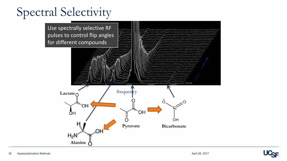
Spectral Selectivity

April 26, 201730

frequency

Pyruvate

13C

Lactate

13C

Bicarbonate

13C

Alanine

13C1

UsespectrallyselectiveRFpulsestocontrolflipanglesfordifferentcompounds


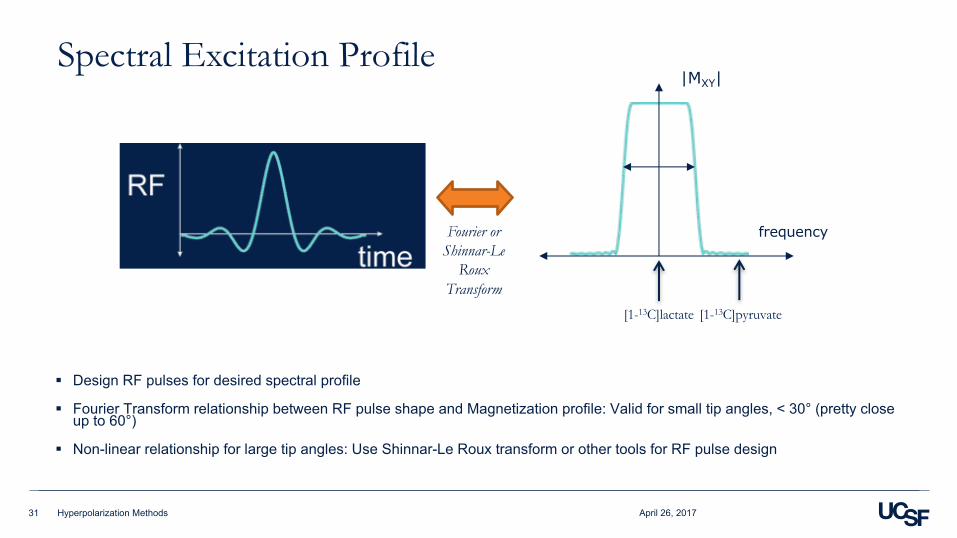
Spectral Excitation Profile

§ Design RF pulses for desired spectral profile

§ Fourier Transform relationship between RF pulse shape and Magnetization profile: Valid for small tip angles, < 30° (pretty close up to 60°)

§ Non-linear relationship for large tip angles: Use Shinnar-Le Roux transform or other tools for RF pulse design

April 26, 201731

frequency

|MXY|

Fourier or Shinnar-Le

Roux Transform

�f

[1-13C]pyruvate[1-13C]lactate


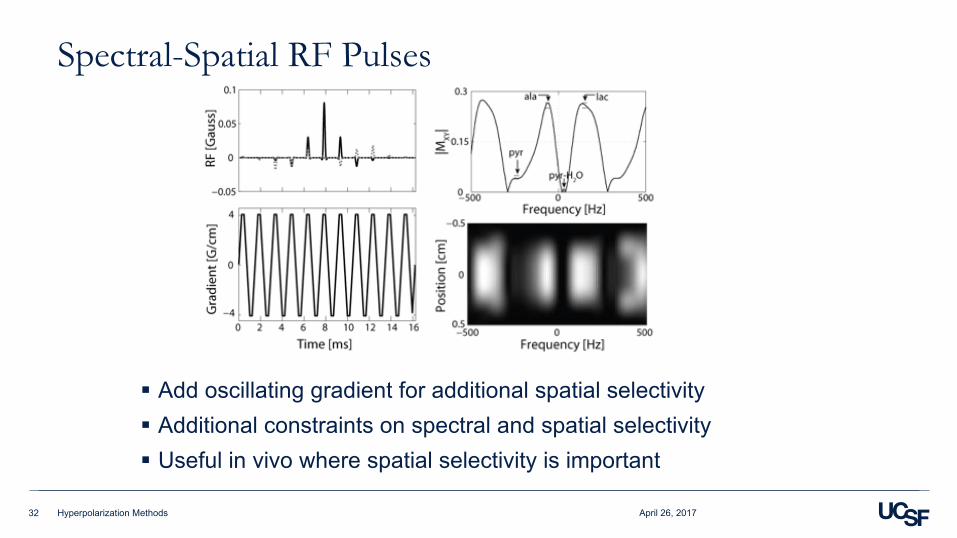
Spectral-Spatial RF Pulses

April 26, 201732

§ Add oscillating gradient for additional spatial selectivity§ Additional constraints on spectral and spatial selectivity§ Useful in vivo where spatial selectivity is important


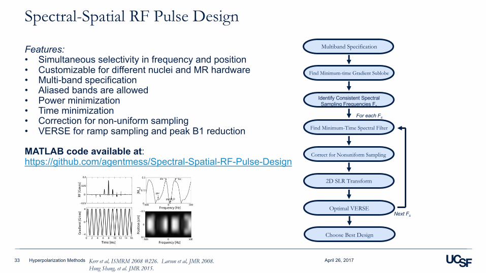
Spectral-Spatial RF Pulse Design

Features:• Simultaneous selectivity in frequency and position• Customizable for different nuclei and MR hardware• Multi-band specification• Aliased bands are allowed• Power minimization• Time minimization• Correction for non-uniform sampling• VERSE for ramp sampling and peak B1 reduction

MATLAB code available at: https://github.com/agentmess/Spectral-Spatial-RF-Pulse-Design

April 26, 201733 Kerr et al, ISMRM 2008 #226. Larson et al, JMR 2008. Hong Shang, et al. JMR 2015.

Find Minimum-time Gradient Sublobe

Identify Consistent Spectral Sampling Frequencies Fs

Find Minimum-Time Spectral Filter

Correct for Nonuniform Sampling

2D SLR Transform

Optimal VERSE

Choose Best Design

Multiband Specification

For each Fs

Next Fs


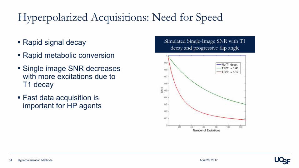
Hyperpolarized Acquisitions: Need for Speed

§ Rapid signal decay

§ Rapid metabolic conversion

§ Single image SNR decreases with more excitations due to T1 decay

§ Fast data acquisition is important for HP agents

April 26, 201734

Simulated Single-Image SNR with T1 decay and progressive flip angle


Readout Strategies

Can be approximately grouped into three categories (from slowest to fastest)

1. MR spectroscopic imaging (MRSI)

2. Model-based Spectral decomposition with multiple TEs (Dixon/IDEAL)

3. MRI with spectrally-selective excitation (“Metabolite-specific Imaging”)


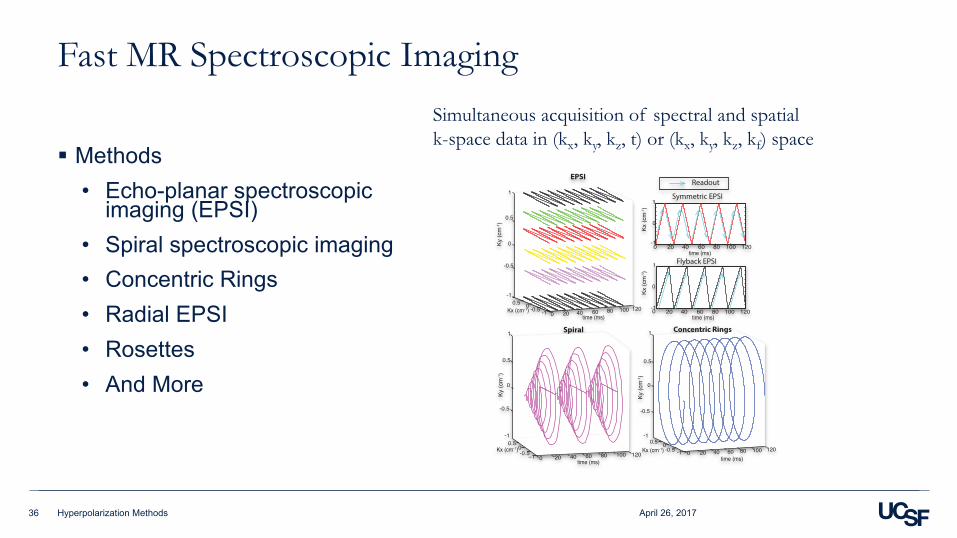
Fast MR Spectroscopic Imaging

§ Methods• Echo-planar spectroscopic

imaging (EPSI)• Spiral spectroscopic imaging• Concentric Rings• Radial EPSI• Rosettes• And More

April 26, 201736

Ky (

cm

-1)

Ky (

cm

-1)

Ky (

cm

-1)

time (ms)

time (ms)time (ms)

Kx (cm-1)

Kx (cm-1)Kx (cm-1)

0 20 40 60 80 100 120−1-0.50

0.5

-1

-0.5

0

0.5

1

0 20 40 60 80 100 120-1

-0.50

0.5-1

-0.5

0

0.5

1

0 20 40 60 80 100 120-1

-0.50

0.5

-1

-0.5

0

1

0.5

-1

0

1

0 20 40 60 80 100 120

0 20 40 60 80 100 120-1

0

1

Symmetric EPSI

Flyback EPSI

Readout

time (ms)

Kx (

cm

-1)

Kx (

cm

-1)

time (ms)

EPSI

Spiral Concentric Rings

Simultaneous acquisition of spectral and spatial k-space data in (kx, ky, kz, t) or (kx, ky, kz, kf) space


MRSI Readouts

April 26, 201737

GZ

DAQ

GZ

kz

kf

kz

kf

DAQ

Phase Encoding

Echo-planar spectroscopic imaging (EPSI)


Accelerated MRSI Strategies

April 26, 201738

Ky (

cm

-1)

Ky (

cm

-1)

Ky (

cm

-1)

time (ms)

time (ms)time (ms)

Kx (cm-1)

Kx (cm-1)Kx (cm-1)

0 20 40 60 80 100 120−1-0.50

0.5

-1

-0.5

0

0.5

1

0 20 40 60 80 100 120-1

-0.50

0.5-1

-0.5

0

0.5

1

0 20 40 60 80 100 120-1

-0.50

0.5

-1

-0.5

0

1

0.5

-1

0

1

0 20 40 60 80 100 120

0 20 40 60 80 100 120-1

0

1

Symmetric EPSI

Flyback EPSI

Readout

time (ms)

Kx (

cm

-1)

Kx (

cm

-1)

time (ms)

EPSI

Spiral Concentric RingsFuruyama J, et al. MRM 2012; 67:1515–1522Jiang, et al, MRM 2016, doi: 10.1002/mrm.25577

Adalsteinsson E, et al. MRM 1998;39:889 – 898.Mayer MRM 2006; 56:932–937.

Yen et al. MRM 2009; 62:1-10.

Ky (

cm

-1)

Ky (

cm

-1)

Ky (

cm

-1)

time (ms)

time (ms)time (ms)

Kx (cm-1)

Kx (cm-1)Kx (cm-1)

0 20 40 60 80 100 120−1-0.50

0.5

-1

-0.5

0

0.5

1

0 20 40 60 80 100 120-1

-0.50

0.5-1

-0.5

0

0.5

1

0 20 40 60 80 100 120-1

-0.50

0.5

-1

-0.5

0

1

0.5

-1

0

1

0 20 40 60 80 100 120

0 20 40 60 80 100 120-1

0

1

Symmetric EPSI

Flyback EPSI

Readout

time (ms)

Kx (

cm

-1)

Kx (

cm

-1)

time (ms)

EPSI

Spiral Concentric Rings


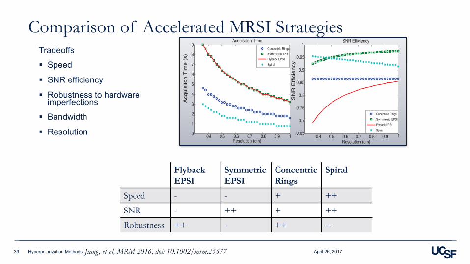
Comparison of Accelerated MRSI StrategiesTradeoffs

§ Speed

§ SNR efficiency

§ Robustness to hardware imperfections

§ Bandwidth

§ Resolution

April 26, 2017390.4 0.5 0.6 0.7 0.8 0.9 1

0

500

1000

1500

2000

2500

3000Spectral Bandwidth

Resolution (cm)

SB

W (

Hz)

Concentric Rings

Symmetric EPSI

Flyback EPSI

Spiral

0.4 0.5 0.6 0.7 0.8 0.9 10

1

2

3

4

5

6

7

8

9Acquisition Time

Resolution (cm)

Acq

uis

ito

n T

ime

(s)

Concentric Rings

Symmetric EPSI

Flyback EPSI

Spiral

0.4 0.5 0.6 0.7 0.8 0.9 10

500

1000

1500

2000

2500

3000Spectral Bandwidth with Interleaves

Resolution (cm)

SB

W (

Hz)

Concentric Rings

Symmetric EPSI

Flyback EPSI

Spiral

0.4 0.5 0.6 0.7 0.8 0.9 10.65

0.7

0.75

0.8

0.85

0.9

0.95

1SNR Efficiency

Resolution (cm)

SN

R E

ffic

ien

cy

Concentric Rings

Symmetric EPSI

Flyback EPSI

Spiral

FlybackEPSI

Symmetric EPSI

Concentric Rings

Spiral

Speed - - + ++

SNR - ++ + ++

Robustness ++ - ++ --

Jiang, et al, MRM 2016, doi: 10.1002/mrm.25577Hyperpolarization Methods

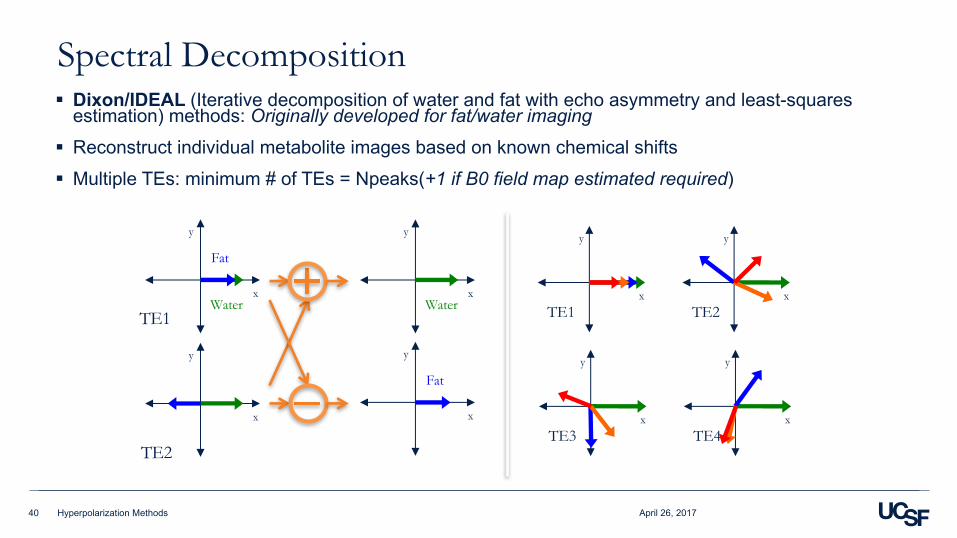
Spectral Decomposition§ Dixon/IDEAL (Iterative decomposition of water and fat with echo asymmetry and least-squares

estimation) methods: Originally developed for fat/water imaging

§ Reconstruct individual metabolite images based on known chemical shifts§ Multiple TEs: minimum # of TEs = Npeaks(+1 if B0 field map estimated required)

April 26, 201740

TE2

x

y

TE1x

y

Fat

Water

x

y

Fat

x

y

Water TE1x

y

TE2x

y

TE3x

y

TE4x

y


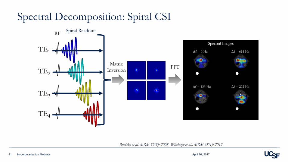
Spectral Images

Δf = 0 Hz Δf = 614 Hz

Δf = 433 Hz Δf = 272 Hz

Spectral Decomposition: Spiral CSI

April 26, 201741

Brodsky et al. MRM 59(5): 2008 Wiesinger et al., MRM 68(1): 2012

RF Spiral Readouts

TE1

TE2

TE3

TE4

Matrix Inversion FFT

SpectralK-space


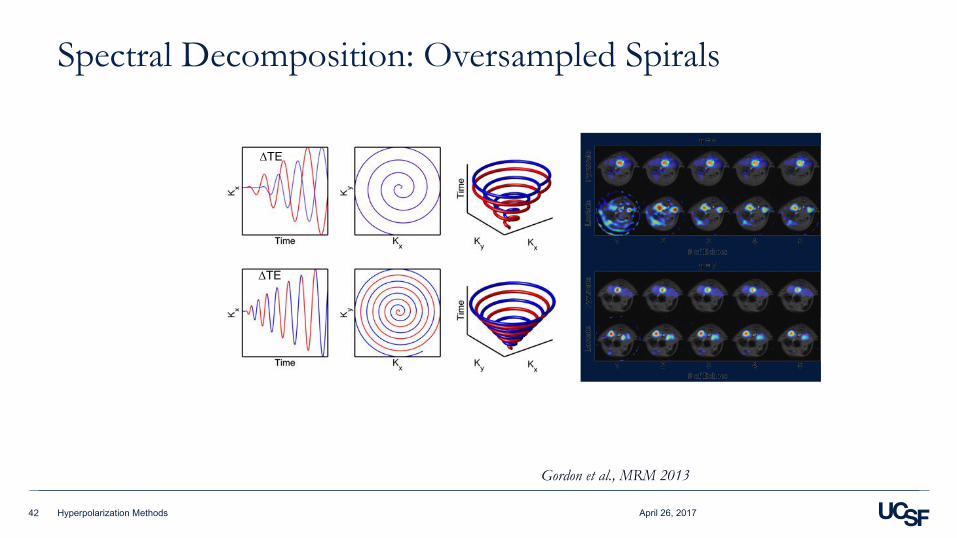
Spectral Decomposition: Oversampled Spirals

April 26, 201742

ΔTE

ΔTECritically

Sampled Spiral (η = 1)

2 echoes

Twice Oversampled Spiral (η = 2)

1 echo

Gordon et al., MRM 2013


Single-shot Spiral MRI

Metabolite-specific Imaging§ Idea: Excite only a single metabolite resonance,

followed by any imaging-based readout§ Methods:

• Single-metabolite Spectral-spatial excitation

• Fast imaging readout (EPI, spiral)

§ Fast!

§ Requires chemical-shift separation of metabolites, sensitive to B0 inhomogeneities

April 26, 201743

Spectral-spatial Excitation

Cunningham JMR 2008. Lau MRM 2010 NMR Biomed 2011


Metabolite-specific Imaging

§ Spectral-spatial excitation of individual metabolites with variable flip angles

§ Ramp sampled, symmetric EPI

§ 16 slices of pyruvate and lactate images in 2 s

April 26, 2017

Cunningham et al. JMR 2008.Gordon et al. MRM 2016. doi: 10.1002/mrm.26123.Gordon et al. Proc ISMRM 2017 #728.

Hyperpolarization Methods44

Clinical Metabolite-specific Imaging

April 26, 2017

Cunningham et al. Circ Res 2016, doi: 10.1161/CIRCRESAHA.116.309769.

a b c10

30

20

20

60

40

5

25

15

80

40

10

50

30

20

60

40

d e f

5 cm 5 cm 5 cm

5 cm 5 cm 5 cm

Pyruvate Bicarbonate Lactate

Pyruvate Bicarbonate Lactate

FIGURE 1

by guest on September 20, 2016

http://circres.ahajournals.org/D

ownloaded from

Cardiac imaging with Spiral Readout

Pyruvate

Lactate

Brain imaging with EPI Readout

Gordon et al. Proc ISMRM 2017 #728.


Technique Comparison

Technique Pros Cons

MRSI Robust to off-resonanceFlexible spectral content

Slow

Spectral Decomposition (IDEAL/Dixon)

Speed+SNR Peak locations must be knownLimits on sequence parameters (TE)

Metabolite-specific Imaging Speed+SNR (max!)Works well with [1-13C]pyruvate spectrum

Sensitive to off-resonanceRequires spectrally separated metabolites


Parametrizations: Kinetic Modeling vs. alternativesNumerous options§ Kinetic modeling (e.g. kPL)§ Lactate/pyruvate§ Area-under-curve (AUCratio, Hill, et al.

PLoS One (2013).)

I advocate for unidirectional kPL model• Insensitive to bolus delivery with any

sampling strategy• Incorporate effects of RF pulses• Compare kPL (1/s) across sites, imaging

protocols, and anatomy• Simple (good for low SNR)

Daniels et al, NMR Biomed 2016, doi: 10.1002/nbm.3468

Hyperpolarization Methods47 April 26, 2017

Choice of Model

§ Models evaluated by Akaike Information Criteria (AIC) which balances fit quality with number of model parameters

a. Pyr-lac (all lumped)

b. Extravascular and intravascular compartments

c. Extravascular/extracellular, intracellular, and intravascular compartments

§ Assumptions

• Neglect kLP, lactate transport. Gamma-variate pyruvate input

• Pyruvate input estimated from heart voxels

• T1P = 45s, T1L = 25s

Bankson et al. Cancer Research 2016. doi: 10.1158/0008-5472.CAN-15-0171


“Input-less” Fitting§ Actual pyruvate signal as input, change in

lactate as output

§ No assumptions or fitting of pyruvate input

§ Pros: Simple, insensitive to fitting errors in pyruvate (e.g. incorrect bolus shape), works with any sampling strategy

§ Cons: No estimate of perfusion

April 26, 2017

Inpsired by: Khegai, et al. NMR Biomed 2014, Bahrami, et al. Quant Imaging Med Surg 2014.


kPL

https://github.com/agentmess/hyperpolarized-mri-toolbox

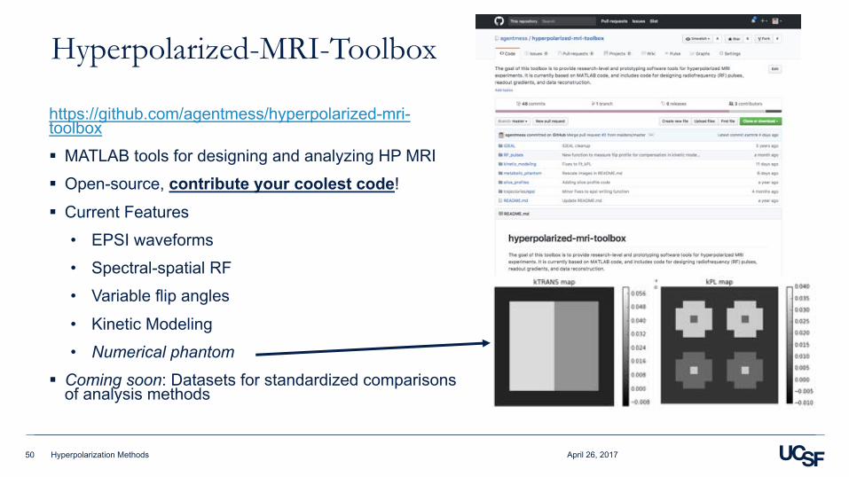
Hyperpolarized-MRI-Toolbox

https://github.com/agentmess/hyperpolarized-mri-toolbox§ MATLAB tools for designing and analyzing HP MRI§ Open-source, contribute your coolest code!

§ Current Features• EPSI waveforms• Spectral-spatial RF• Variable flip angles

• Kinetic Modeling• Numerical phantom

§ Coming soon: Datasets for standardized comparisons of analysis methods


hyperpolarization -description, overview & method · para-hydrogen induced polarization (phip)...

Documents