hyperon interaction in free space and nuclear matter...

Hyperon Interaction in Free Space and Nuclear

Matter Within a SU(3) Based Meson Exchange

Model

Dissertation

zur Erlangung des Grades eines

Doktors der Naturwissenschaften

(Dr. rer. nat.)

Madhumita Dhar

aus Cooch-Behar, Indien

Institut fur Theoretische Physik

Justus-Liebig-Universitat

Gießen, Germany

June, 2016

Dekan: Prof. Dr. Bernhard Muhlherr

Betreuer: Prof. Dr. Horst Lenske

Erstgutachter: Prof. Dr. Horst Lenske

Zweigutachter: Prof. Dr. Christian Fischer

To my parents

“It always seems impossible until its done.”

Nelson Mandela

Abstract

To establish the connection between free space and in-medium hyperon-nucleon in-

teractions is the central issue of this thesis. The guiding principle is flavor SU(3)

symmetry which is exploited at various levels. In first step hyperon-nucleon and

hyperon- hyperon interaction boson exchange potential in free space are introduced.

A new parameter set applicable for the complete baryon octet has been derived

leading to an updated one-boson- exchange model, utilizing SU(3) flavor symmetry,

optimizing the number of free parameters involved, and revising the set of mesons

included. The scalar, pseudoscalar, and vector SU(3) meson octets are taken into

account. T-matrices are calculated by solving numerically coupled linear systems of

Lippmann-Schwinger equations obtained from a 3-D reduced Bethe-Salpeter equa-

tion. Coupling constants were determined by χ2 fits to the world set of scattering

data. A good description of the few available data is achieved within the imposed

SU(3) constraints.

Having at hand a consistently derived vacuum interaction we extend the ap-

proach next to investigations of the in-medium properties of hyperon interaction,

avoiding any further adjustments. Medium effect in infinite nuclear matter are

treated microscopically by recalculating T-matrices by an medium-modified system

of Lippmann-Schwinger equations. A particular important role is played by the Pauli

projector accounting for the exclusion principle. The presence of a background me-

dium induces a weakening of the vacuum interaction amplitudes. Especially coupled

channel mixing is found to be affected sensitively by medium. Investigation on scat-

5

6

tering lengths and effective range parameters are revealing the density dependence

of the interaction on a quantitative level.

Abstrakt

Der zentrale Aspekt dieser Arbeit ist es die Beziehung zwischen der Hyperon-

Nukleon Wechselwirkung im Vakuum und Medium herzustellen. Das Leitprin-

zip ist die SU(3) flavour Symmetrie die auf verschiedenen Levels Verwendung fin-

det. In einem ersten Schritt werden die Bosonenaustauschpotentiale der Hyperon-

Nukleon und Hyperon-Hyperon Wechselwirkung eingefuhrt. Ein neuer Paramet-

ersatz, welcher fur das gesamte Baryon-Oktett anwendbar ist wurde bestimmt, was

unter Benutzung der SU(3) flavour Symmetrie, Optimierung der Anzahl beteiligter

freier Parameter und Uberarbeitung des einbezogenen Satzes an Mesonen zu einem

aktualisierten Einbosonaustausch-Modell fuhrt. Die skalaren, pseudoskalaren und

vektoriellen SU(3) Meson-Oktetts sind berucksichtigt. T-Matrizen sind durch das

numerische Losen gekoppelter, linearer Systeme von Lippmann-Schwinger-Gleichungen,

erhalten aus einer dreidimensionalen reduzierten Bethe-Salpeter-Gleichung, berech-

net. Kopplungskonstanten wurden durch einen χ2-Fit an den weltweiten Satz an

Streudaten bestimmt. Eine gute Beschreibung der wenigen, verfugbaren Daten ist

innerhalb der auferlegten SU(3) Bedingungen erreicht.

Mit einer konsistent bestimmten Vakuumwechselwirkung zur Hand, erweitern wir

den Ansatz, unter Vermeidung irgendwelcher weiterer Anpassungen zu Untersuchun-

gen der Mediumseigenschaften der Hyperonwechselwirkung. Mediumseffekte in un-

endlicher Kernmaterie sind mikroskopisch durch die Neuberechnung der T-Matrizen

durch ein mediumsmodifiziertes System von Lippmann-Schwinger-Gleichungen be-

handelt. Eine besonders wichtige Rolle spielt der Pauli-Projektor, welcher das Aus-

schlussprinzip berucksichtigt. Das Vorhandensein eines Hintergrundmediums be-

7

8

wirkt eine Abschwachung der Vakuumswechselwirkunsgamplituden. Es stellt sich

heraus, dass insbesondere die Mischung gekoppelter Kanale durch das Medium em-

pfindlich beeinflusst ist. Die Untersuchungen von Streulangen und Parametern der

effektiven Reichweite enthullen die quantitative Dichteabhangigkeit der Wechsel-

wirkung.

Contents

1 Introduction 191.1 Strong Interaction . . . . . . . . . . . . . . . . . . . . . . . . . . . . . 19

1.1.1 Properties of Nuclear Forces . . . . . . . . . . . . . . . . . . . 201.2 Pathway to Hyperon Interaction . . . . . . . . . . . . . . . . . . . . . 221.3 Current Approaches . . . . . . . . . . . . . . . . . . . . . . . . . . . . 24

1.3.1 Lattice QCD approaches . . . . . . . . . . . . . . . . . . . . . 241.3.2 Meson Exchange Models . . . . . . . . . . . . . . . . . . . . . 251.3.3 Chiral (χ) Effective Field Theory . . . . . . . . . . . . . . . . 261.3.4 Quark Cluster Model . . . . . . . . . . . . . . . . . . . . . . . 26

1.4 Framework Used in This Thesis . . . . . . . . . . . . . . . . . . . . . 27

2 Interaction Model Description 292.1 SUf (3) Flavor Symmetry . . . . . . . . . . . . . . . . . . . . . . . . . 30

2.1.1 Baryon and Meson Representations in SUf (3) . . . . . . . . . 332.2 Interaction Lagrangian . . . . . . . . . . . . . . . . . . . . . . . . . . 35

2.2.1 Field Theoretical Description . . . . . . . . . . . . . . . . . . 362.2.2 Meson Exchange Forces . . . . . . . . . . . . . . . . . . . . . 36

2.3 Effective Model Parameters . . . . . . . . . . . . . . . . . . . . . . . 402.3.1 Meson Masses . . . . . . . . . . . . . . . . . . . . . . . . . . . 402.3.2 Coupling Constants . . . . . . . . . . . . . . . . . . . . . . . . 422.3.3 Octet-Octet and Octet-Singlet Interaction . . . . . . . . . . . 442.3.4 SUf (3) Baryon-Baryon-Meson vertices . . . . . . . . . . . . . 452.3.5 Free Parameters . . . . . . . . . . . . . . . . . . . . . . . . . . 48

2.4 Comparison with Contemporary Models . . . . . . . . . . . . . . . . 502.5 Summary of the model . . . . . . . . . . . . . . . . . . . . . . . . . . 52

3 Scattering Theory and Formalism 533.1 Kinematics . . . . . . . . . . . . . . . . . . . . . . . . . . . . . . . . 54

3.1.1 Relativistic kinematics of Two-particle Scattering . . . . . . . 543.2 Scattering Equations . . . . . . . . . . . . . . . . . . . . . . . . . . . 57

3.2.1 Bethe-Salpeter Equation . . . . . . . . . . . . . . . . . . . . . 573.2.2 Lippmann-Schwinger Equation . . . . . . . . . . . . . . . . . 60

3.3 Isospin Basis . . . . . . . . . . . . . . . . . . . . . . . . . . . . . . . . 613.4 Coupled Channel Formalism . . . . . . . . . . . . . . . . . . . . . . . 64

9

10 CONTENTS

3.5 Formation of the Potential . . . . . . . . . . . . . . . . . . . . . . . . 683.5.1 OBEP Amplitudes . . . . . . . . . . . . . . . . . . . . . . . . 693.5.2 Potential Matrix in Isospin Basis . . . . . . . . . . . . . . . . 78

3.6 Introduction to Particle Basis . . . . . . . . . . . . . . . . . . . . . . 79

4 Numerical Methods 854.1 R-Matrix . . . . . . . . . . . . . . . . . . . . . . . . . . . . . . . . . 854.2 Representation in Partial Wave Basis . . . . . . . . . . . . . . . . . . 86

4.2.1 Partial Wave Amplitude . . . . . . . . . . . . . . . . . . . . . 874.2.2 Partial Wave Projection of Potential Elements . . . . . . . . . 914.2.3 Partial Wave Integral Equation . . . . . . . . . . . . . . . . . 92

4.3 Numerical Formalism for R-matrix Solution . . . . . . . . . . . . . . 944.3.1 Extraction of T-matrix from R-matrix . . . . . . . . . . . . . 97

4.4 Determination of Observables . . . . . . . . . . . . . . . . . . . . . . 994.4.1 Cross Section . . . . . . . . . . . . . . . . . . . . . . . . . . . 994.4.2 Phase Shift . . . . . . . . . . . . . . . . . . . . . . . . . . . . 1004.4.3 Low-Energy (LE) Parameters . . . . . . . . . . . . . . . . . . 101

5 Vacuum Hyperon-Baryon Interactions 1055.1 Sensitivity of Parameters . . . . . . . . . . . . . . . . . . . . . . . . 105

5.1.1 Fitting Procedure . . . . . . . . . . . . . . . . . . . . . . . . . 1075.2 Result of Fit . . . . . . . . . . . . . . . . . . . . . . . . . . . . . . . . 1165.3 Free Space Result . . . . . . . . . . . . . . . . . . . . . . . . . . . . . 121

5.3.1 S = 0 Results . . . . . . . . . . . . . . . . . . . . . . . . . . . 1225.3.2 S = -1 Results . . . . . . . . . . . . . . . . . . . . . . . . . . . 126

5.3.2.1 Uncoupled Channels . . . . . . . . . . . . . . . . . . 1275.3.2.2 Coupled Channels . . . . . . . . . . . . . . . . . . . 128

5.3.3 S = -2 Results . . . . . . . . . . . . . . . . . . . . . . . . . . . 1395.4 Dependence of the LE Parameters on the Coupling Constants . . . . 1415.5 Summary of Free Space Interaction . . . . . . . . . . . . . . . . . . . 142

6 In-Medium Effect 1476.1 Baryon-Baryon Interaction in Infinite Nuclear Matter . . . . . . . . . 148

6.1.1 In-Medium Bethe-Goldstone Equation . . . . . . . . . . . . . 1486.1.2 Pauli Projector Operator . . . . . . . . . . . . . . . . . . . . . 1506.1.3 Transformation to Center-of-Mass Frame . . . . . . . . . . . . 151

6.2 Hyperon Mean Fields . . . . . . . . . . . . . . . . . . . . . . . . . . . 1556.3 In-medium Phase Shift and Cross Section . . . . . . . . . . . . . . . . 1566.4 In-medium Low-Energy Parameters . . . . . . . . . . . . . . . . . . . 1616.5 Medium Effect vs. Parameter Variation . . . . . . . . . . . . . . . . . 1666.6 Conclusion . . . . . . . . . . . . . . . . . . . . . . . . . . . . . . . . . 167

7 Summary and outlook 171

Appendices 175

A Coupling Constant Values 177

CONTENTS 11

B Partial Wave Potential Matrix Elements 179

C LSJM Representation Operators 183

D Partial Wave Decomposition of NN 187

E Helicity State Basis Decomposition 189

Bibliography 192

Preface

“Not only is the Universe

stranger than we think, it is

stranger than we can think. ”

Werner Heisenberg

About a century ago, microscopic physics started with the demand of under-

standing atomic spectra. That effort gave rise to the invention of quantum mech-

anics, the key science of our time. From the present day’s point of view, theoretical

as well as experimental studies of atoms and molecules have become standard work,

reaching even deep into the industrial and commercial sectors. That is because those

systems exist under the action of the meanwhile well known electromagnetic laws of

force.

In nuclear and hadron physics, however, we have not yet reached a comparable

state of knowledge. In addition to the complexities of quantum mechanics, nuclear

physics is governed by the strong force which in its low energy realization is a

highly complicated non-perturbative phenomenon. While the nuclear sector has

taken a large step forward to produce a good number of successful, realistic, high-

precision models [10, 11, 55, 62, 64, 110] utilizing a rich data set available with

simultaneous computational progress, the strange nuclear physics is still far behind.

The main constraint is the lack of even a sufficient number of experimental data

that makes it difficult to have a unique understanding. There are several attempts

made to construct to construct an unique interaction, in both relativistic and non-

13

14 CONTENTS

relativistic framework, however the combined effort failed to close the open problem

on hyperons. This being one scenario, the oner is more compelling for physicists to

take this issue under re-investigation.

The present available interaction models include the meson exchange approaches

of the groups from Nijmegen [49, 50](NSC, ESC) and Julich [46–48], respectively,

the Kyoto-Niigata model based on the quark cluster framework (Fss2) [105], the

Lattice QCD descriptions [44, 45] using numerical simulations based on Quantum

Chromo Dynamics (QCD), and the latest addition to this list is chiral perturbation

theory extended to the SU(3) flavor sector, also known as chiral effective field theory

(χEFT) [100], which is accounting for QCD symmetries and applying a systematic

order-by-order scheme on the diagrammatic level. However, most of the results are in

contradiction to one another in many key points and as of now none of the framework

can deal simultaneously from S = 0 to S = -4 strangeness sector without extra

modifications accounting for the the complexities introduced by higher strangeness

involved. Sophisticated approaches like χEFT [100] and Lattice QC [44, 45] are still

under construction for the higher strangeness channels to a satisfactory level.These

issues emphasizes that to construct a single line theory for the hyperon interactions

is a demanding task. The special characteristics of hyperon-related problems is

multi-channel physics which is an important aspect goes much beyond the level of

complexity encountered in the Nucleon-Nucleon (NN) case.

Recent observation of different exotic systems such as 6ΛH [1], unexpected short-

lifetime of hypertriton [2], strong indication towards the existence of only-charge

neutral nnΛ bound state [3], also supported by recent hyper-nuclear and hyper-

matter results from RHIC and LHC [4, 5] are not yet being understood under the

present hyperon interaction framework available. On the other hand, a number of

strangeness experiments has been planned to perform in near future in J-PARC (Ja-

pan), CLAS12 at J-LAB (USA), PANDA (Germany) , KaoS at MAMI (Germany)

and FINUDA and DAΦNE (Italy) that will require of course a realistic hyperon

interaction scheme for proper interpretation. The hyper physics program leading by

Take Saito et. al ar FRS at GSI that is upgraded to SUPERFRS at FAIR in the

upcoming facility will also be an important laboratory for hyper-nuclear physics.

CONTENTS 15

All these together demand for a reconsideration of the existent models, with a more

elaborate frame work. We therefore decided to take this issue as our research topic

with attention to the unsolved problems. Therefore, we will construct a revised va-

cuum interaction model for hyperons in this thesis that can be applied to investigate

all the above mentioned phenomena in a consistent manner.

While vacuum interaction information is fundamental, to complete the know-

ledge base, there is additional requirement towards investigation of in-medium hyp-

eron interaction as well. The major drawback for obtaining experimental data for

hyperons is their short-lifetime that make is impossible to make a hyperon beam.

Only possible option to have hyperons are therefore as by-product from other pro-

cesses. High energy hadronic reactions are one such tool that provides the oppor-

tunity to have hyperons as final fragments. On the contrary to beam-target type

accelerator experiments, these kind of production method come up with a large

background. For the heavy ion collisions the background is mainly nuclear medium.

The recent two solar mass neutron star [89, 90] observation started the present day

discussed ”hyperon puzzle” of neutron stars. The high mass limit sets a strong con-

Figure 1: Baryon particle fraction as a function of baryon density. Figure taken from [91]

straint on the type of equation of state (EoS) being able to reproduce neutron stars

the highest observed masses. The inclusion of hyperons softens the EoS, making it

difficult to reach the two-solar-mass region at least with the standard parameter sets

16 CONTENTS

[7]. An additional uncertainty is introduced by the open question if in the interior

of a neutron star a transitions into a new quark matter phase occurs. However,

there is still not a full proof answer to the question of whether hyperon degrees of

freedom are present inside neutron stars or not. The puzzle arises since at such high

densities hyperons are most likely to be present in neutron star core as shown for

example in the baryon particle fraction plot as a function of density, taken from [91],

although the result is model dependent, however it does give an idea that hyperons

are most likely to appear already well below neutron star typical densities, which is

about 5 times nucleon saturation density. Thus, inclusion of hyperons not producing

two-solar-mass is emerging as the hyperon puzzle.

This created a quest for hyperon interaction at high baryon densities within a

realistic interaction framework. A number of phenomenological approaches have

pointed towards ad-hoc vector meson exchange [94], multi pomeron exchange [95],

even in particular adjusting the Λ-nucleon three-body interaction [41]. More sys-

tematic investigation is therefore mandatory to solve this puzzle. In this thesis,

we, therefore considered the medium effect study of hyperon bare interaction as our

second part of work.

Figure 2: Mass-Radius diagram of different neutron star models. Only steep EoS can reach upto two solar masses. Figure taken from [92]

CONTENTS 17

There exists a number of methods like Dirac-Brueckner Hartree-Fock calculation

[32], G-matrix calculation [19], density functional theory [34, 35] etc. for investigat-

ing the medium effect. Most of these methods are based in mean-filed frame work,

relativistic [108, 109], or non-relativistic [86]. The mean-field framework does not

need information about the bare interaction. For a microscopic in-medium interac-

tion, on the other hand, the in-medium effect is applied on the free space interaction,

by Brueckner theory. Brueckner theory is largely used for nuclear sector already.

Extension of the same to include hyperons was done first in the nineties by [87, 88].

The advantage of a microscopic theory over these mean field models is obvious,

providing more insights already from the bare interaction level. With the aim of

constructing a consistent realistic free space hyperon interaction as first task, we

can readily study in-medium properties with necessary modification microscopically.

Thus, our investigation is divided in to two parts: first we will present a realistic

hyperon interaction for vacuum, which then we will use for investigating hyperon

in-medium property research. In this thesis, we restrict ourselves at this stage up to

nuclear matter densities for in-medium effect study of the bare interaction, pointing

out the possibility to extend to other exotic systems with relevant mechanism.

Some of the results presented in this thesis are published in:

”Exotic nuclear matter”, Horst Lenske, Madhumita Dhar, Nadja Tsoneva, Jonas

Willhelm, EPJ Web Conf. 107 (1026) 10001;

”Hyperon Interaction in Free Space and Nuclear Matter”, The 12th International

Conference on Hypernuclear and Strange Particle Physics (HYP2015) Conference

Proceedings, 7-11 September, 2015, Sendai, Japan, [arXiv:1603.00298];

”Hyperon Interaction in Nuclear matter and Neutron Star”, GSI Scientific Re-

port 2014;

”SU(3) Approach to Hypernuclear Interactions and Spectroscopy”, Horst Lenske,

Madhumita Dhar, Theodoros Gaitanos, submitted to Nuclear Physics A for public-

ation, [arXiv:1602.08917],

and the rest of the results are in preparation.

The thesis is organized as follows:

Chapter 1: A general review of strong interaction is given. The contemporary

18 CONTENTS

models and theories for hyperon interaction are reviewed briefly. Finally the

need of a revised approach is explained in connection with this work.

Chapter 2: The interaction model used in this work is explained in detail.

Chapter 3: This chapter contains information about two- body scattering the-

ory. The two-body covariant Bethe-Salpeter equation is discussed in connec-

tion to hyperon interaction. One-boson-exchange potential amplitudes used

in this work are described in detail. Various representation basis schemes of

baryon-baryon scattering channels are also a part of discussion of the chapter.

Chapter 4: This chapter deals about numerical formalism of our research. A

description of the partial wave decomposition of scattering equation is given,

followed by the numerical methods adopted to solve the scattering equation

is explained first, finishing with a description on determination of relevant

scattering observables numerically.

Chapter 5: Results for the vacuum baryon-baryon interaction is presented.

Chapter 6: The effect of nuclear - medium on the vacuum interaction is shown.

Chapter 7: A brief summary and future outlook are the topics of this chapter.

Chapter 1Introduction

“The important thing is to not

stop questioning. Curiosity has

its own reason for existence.”

Albert Einstein

In this chapter, a general review about strong hyperon interaction has been given.

In Section 1 the aspects of strong interaction is described, which must be followed by

hyperon interaction. Section 2 is devoted to describe the known properties of nuclear

force. In Section 3 few words on hyperon discovery and the properties observed till

date are mentioned. The various interaction models active in this field that are

mentioned briefly in Section 4. In Section 5 reasons for deriving a revised a vacuum

interaction approach has been highlighted.

1.1 Strong Interaction

Both hyperons and nucleons belong to the same group of particles: the baryons.

Both of the particles are part of the baryon octet and strongly interacting particles.

This ensures a basic similarity must lie between their interactions with of course a bit

of difference owing to the strange and non-strange quark presence. There are a large

number of non-strange stable nuclei available that allows to do nucleon scattering

experiments. On the other hand, hyperon scattering experiments are very difficult

due to the short life time of hyperons. This makes hyper nuclear physics as the most

19

20 CHAPTER 1. INTRODUCTION

difficult branch of nuclear physics. In order to proceed, one can use the information

obtained from the nucleon scattering experiments, which effectively helped to gain

an understanding about the basic features of the strong interaction, in particular

the nuclear force.

1.1.1 Properties of Nuclear Forces

Nuclear force is what holds the nucleons together inside the nucleus. There are three

types of nuclear interactions: strong, weak and electro magnetic. As far as strong

interaction is concerned, the force between two nucleons is the most prominent

example on this front. Over the last century there has been a great number of

theoretical and experimental research that adds up to the understanding of strong

interaction properties. The basic properties of the nuclear forces that are known until

today are compiled in many papers [20]. The nature of nuclear forces is studied by

analyzing the properties of the nuclei. The empirical features of nuclear force are

listed as the followings:

1. Short range: Nuclear force is of short range nature. Rutherford’s famous

alpha particle scattering experiment showed the range of nuclear force to be of

the order of 10−15 m. The range is usually upto 1-2 fm. The nearly constant

values of the binding energy per nucleon (Fig. 1.1) and the density supports

the finite short range behavior. This is also evident from the fact that the

interactions between nuclei in a molecule are entirely described by Coulomb

force.

2. Stronger than Coulomb force at short distances: The strength of the

force is stronger than the Coulomb force at this order, otherwise it would not

have been possible to keep the protons together in presence of the Coulomb

repulsion among them.

3. Short range repulsion: The short range repulsion part of the strong force

is the most interesting yet challenging one. This is usually is referred as the

’repulsive core’ or simply ’hard core’. The repulsive core is usually over the

distance 0.5 fm. This means the nucleons cannot go closer beyond that.

1.1. STRONG INTERACTION 21

4. Intermediate range attraction: Outside the repulsive core, nuclear force

must be attractive in nature otherwise one can not have nucleus. Nucleon-

nucleon (NN) scattering experiments showed positive S-wave phase shifts (im-

plying attraction) for low energies as a proof of this.

5. Saturation: The saturation property is coming from the fact of nearly con-

stant binding energy per nucleon (B.E/A) ≃ 8.5 MeV for nuclei above A > 4

[Fig. 1.1].

Figure 1.1: Binding Energy per Nucleon vs mass number plot. Binding energy per nucleonclearly shows a saturation behavior. Figure copyright [6].

6. Spin dependence: For deuteron, only spin 1 state is bound. Different isospin

states of spin 0 shows different phase shift. To conclude, nuclear force depends

both on spin and isospin.

7. Non - central tensor force: The deuteron has a non-zero magnetic and

quadrupole moment, which implied the shape being not spherical. This fact

can be explained by postulating deuteron as an admixture of S-state and D-

state. Tensor force hence come into play a role here as the tensor operator

defined in coordinate space here as

S12 = 3(σ1 · r12)(σ2 · r12)− (σ1 · σ2) (1.1)


can mix states with different orbital angular momentum (L) where σ1 and σ2

are the spins of particle 1 and 2 respectively and r12 is the unit vector along

the direction of relative distance between particle 1 and 2.

8. Spin - orbit force: Nuclear spectra showed evidence on the dependence of

nuclear force on spin-orbit (L.S) force.

9. Charge independence: Nuclear force is charge symmetric. This implies that

if one exchange the overall number of protons with neutrons and vice-versa,

the force will remain unaltered. The similarity in the excitation spectra of the

mirror nuclei also is a consequence of the charge symmetry of strong force.

10. Exchange of charge : Nuclear force can exchange charge. From neutron-

proton scattering experiments, a forward as well as a backward peak has been

seen. The backward peak is interpreted as actually a neutron being converted

to a proton being scattered. Beta-decay is also another example of the charge

-exchange reaction.

11. Symmetry principles: Lastly the force must follow the basic invariance

principles: translation, Galilei, rotation, parity, and time -reversal.

1.2 Pathway to Hyperon Interaction

In 1947, Rochester and Butler reported the appearance of forked tracks due

to associated production of a pair of unstable particles [122]. These tracks were

experimentally soon discovered as referring to pair production of particles, K-meson

and Λ. This was the first discovery of a strange particle and marked the beginning

of strangeness era in physics. These new particles were termed ’strange’ due to the

two peculiar behaviors of their tracks: these particles were always observed to be

produced in ’pairs’ by ’fast’ strong interaction processes, and found to decay by a

’slow’ process. The puzzle at that time was why the particles which were produced

by strong interaction, always decayed by weak interaction, later indebted as the

characteristics of particles carrying the new quantum number S for strangeness.

1.2. PATHWAY TO HYPERON INTERACTION 23

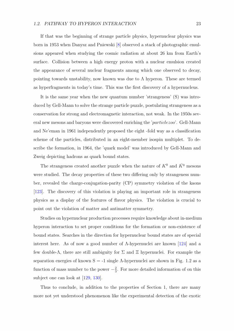
If that was the beginning of strange particle physics, hypernuclear physics was

born in 1953 when Danysz and Pniewski [8] observed a stack of photographic emul-

sions appeared when studying the cosmic radiation at about 26 km from Earth’s

surface. Collision between a high energy proton with a nuclear emulsion created

the appearance of several nuclear fragments among which one observed to decay,

pointing towards unstability, now known was due to Λ hyperon. These are termed

as hyperfragments in today’s time. This was the first discovery of a hypernucleus.

It is the same year when the new quantum number ’strangeness’ (S) was intro-

duced by Gell-Mann to solve the strange particle puzzle, postulating strangeness as a

conservation for strong and electromagnetic interaction, not weak. In the 1950s sev-

eral new mesons and baryons were discovered enriching the ’particlezoo’. Gell-Mann

and Ne’eman in 1961 independently proposed the eight -fold way as a classification

scheme of the particles, distributed in an eight-member isospin multiplet. To de-

scribe the formation, in 1964, the ’quark model’ was introduced by Gell-Mann and

Zweig depicting hadrons as quark bound states.

The strangeness created another puzzle when the nature of K0 and K0 mesons

were studied. The decay properties of these two differing only by strangeness num-

ber, revealed the charge-conjugation-parity (CP) symmetry violation of the kaons

[123]. The discovery of this violation is playing an important role in strangeness

physics as a display of the features of flavor physics. The violation is crucial to

point out the violation of matter and antimatter symmetry.

Studies on hypernuclear production processes require knowledge about in-medium

hyperon interaction to set proper conditions for the formation or non-existence of

bound states. Searches in the direction for hypernuclear bound states are of special

interest here. As of now a good number of Λ-hypernuclei are known [124] and a

few double-Λ, there are still ambiguity for Σ and Ξ hypernuclei. For example the

separation energies of known S = -1 single Λ-hypernuclei are shown in Fig. 1.2 as a

function of mass number to the power −23. For more detailed information of on this

subject one can look at [129, 130].

Thus to conclude, in addition to the properties of Section 1, there are many

more not yet understood phenomenon like the experimental detection of the exotic


Figure 1.2: Separation energies of known S = -1 single Λ-hypernuclei as a function of massnumber to A− 2

3 . Figure taken from [129]

hyperon systems, short life-time, multi-channel transfer reactions, effect on highly

dense objects like neutron star on hyperon physics, which are typical to hyperon

physics. To conclude, there are still many open questions in this subject that is worth

attempting for investigations with a consistent hyperon interaction framework.

1.3 Current Approaches

Before introducing our interaction model, we first briefly summarize the till

date existent models or frameworks aiming to calculate hyperon-baryon interac-

tions. There are mainly four approaches used to treat this problem: Lattice QCD

(Quantum Chromo Dynamics) [44, 45], meson-exchange models [46–50], chiral ef-

fective field theory, (χEFT) [100, 101, 106], and quark -cluster models [105]. In the

following we highlight the key aspects of these frameworks.

1.3.1 Lattice QCD approaches

Quantum Chromodynamics (QCD) is the fundamental theory of strong interaction

governing the interaction of baryons. However, field theoretical description of the

baryon interaction should start from quark degrees of freedom as the QCD Lag-

rangian needs description of quark-gluon dynamics. The non-perturbative nature

of QCD at hadron degrees of freedom therefore makes the solution of QCD Lag-

rangian very much involved, making the analytical solution technique impossible.

1.3. CURRENT APPROACHES 25

Lattice QCD framework provides an alternative simulation technique to this. The

QCD path integral is calculated in a finite four-dimensional discretized Euclidean

or Minkowski box with a shortest length scale, known as the lattice-spacing, thus

discretizing space and time to evaluate the integral in a finite volume. Quantum

Monte Carlo integration is used to perform the path integral. At present only simu-

lations with fairly large quark masses, small volumes, and large lattice spacings are

achievable for full QCD due constraint coming from computer computation limit.

Due to the excessive time consuming calculations, the progress in lattice QCD sector

is rather slow compared to other effective frameworks involved.

Different type of QCD simulations like quenched and (2+1)-flavor has been car-

ried out by HAL-QCD [44] and NPLQCD [45] collaborations for ΛN and ΣN sys-

tems already, with preliminary calculations for S = -2 by [44]. Extension to higher

strangeness channels are in progress. However, the present pion mass used in this

calculations is still far from physical point usually of the order of 300-400 MeV. In

any event, simulation results from lattice QCD play an important role in providing

additional constraints in hyperon physics with large ambiguity.

1.3.2 Meson Exchange Models

Days since Yukawa predicted meson exchange theory, meson exchange has been

employed extensively to construct baryon potentials. The exchanged mesons in

meson-exchange models playing the same role as photons in electrodynamics. The

meson-exchange potentials has been proven to be very successful for phenomeno-

logical determination of nuclear forces [10, 11, 55, 64]. The high-precision Bonn

nuclear potential has been successfully extended to include hyperons by the Julich

group in the late eighties [46], further modified to two more versions [47, 48] all

utilizing SU(6) symmetry of quarks. The Julich has their last version applicable for

S = -1 sector with no more further advancement provided from the authors.

The Nijmegen nucleon potential is modified to include hyperons using SU(3)-

flavor symmetry with mass breaking effects explicitly included. Different version

available from Nijmegen groups differing on the core interaction , hard or soft one

[49, 50]. One specific feature if Nijmegen group of potentials is their inclusion of


fictitious particle pomeron in their models. The Nijmegen strange potentials has

different versions, with a large set of variation within their own framework both

published and unpublished with a version available for complete baryon octet [49]

with many other versions available as applied versions to S = -1, S = -2 [50, 51].

1.3.3 Chiral (χ) Effective Field Theory

An alternative theory in nuclear physics is discovered recently in the last decade,

namely the chiral effective field theory. The framework is based on a modified Wein-

berg power counting incorporating the QCD symmetries explicitly into the scheme.

Similar to meson-exchange models, the EFT framework too assumes the validity of

SU(3)-flavor symmetry for the hyperon-nucleon interaction. The framework has the

option of systematic improvements by including higher order terms by perturbative

expansion, known as leading order (LO), next-to-leading-order (NLO) and so on.

The Julich-Bonn-Munich [100, 101, 106] group is extensively working on this sub-

ject. The diagrams contributing for EFT theory are calculated analytically first by

power counting. For higher order the number of diagrams increases, hence making

the task quite cumbersome. The short-range part on the interaction in χEFT is

attributed by four-baryon contact terms, that are fixed by fit to data. The contact

terms derived here are imposed with SU(3)-flavor constraints to reduce free para-

meters. For the LO version [106], the long-range part consists of one-pseudo-scalar

meson exchange and for NLO [101], two-pseudo scalar meson exchange diagrams

are also included. At present S = -2, -3, -4 results are available up to LO [100]

and only S = -1 extended up to NLO [101]. The results obtained are pretty good

in describing the hyperon-nucleon data with uncertainty involved equivalent to the

present meson-exchange models. Thus, the EFT scheme is a good alternative theory

to study the hyperon-interaction in general.

1.3.4 Quark Cluster Model

In quark cluster model [105] valence quarks are the force mediators. The Hamilto-

nian here consists of three parts: quark kinetic energy, quark confinement potential,

1.4. FRAMEWORK USED IN THIS THESIS 27

and residual quark-quark interactions. The short- range core here is derived from

the color-magnetic gluon exchange and the quark anti-symmetrization in the valence

quark dynamics. In a hybrid version of the model, low-lying mesons were also in-

cluded to describe the long-range interaction part. In this framework, contrary to

meson-exchange picture, the mesons can also interact with the quarks inside bary-

ons. The meson-baryon couplings used for the calculations are usually taken from

Nijmegen potential. The results obtained from this scheme in many cases differ from

the other three mentioned earlier and in general not preferred for further application.

1.4 Framework Used in This Thesis

In this work, we will follow the conventional meson-exchange scheme to construct

our own bare interaction model. Due to the present uncertainty in the level of OBE

parameter sets used by the OBE hyperon models, increasing strangeness leads to

change in the parameters involved for better quantitative analysis of the observables.

Moreover, the two groups differ in their preference in symmetry consideration as

discussed earlier. With this being the case, we are interested in a qualitative study

of the validity of SU(3)-flavor symmetry in the baryon-baryon octet sector. As a

consequence we do not want to not include any other mesons as mediators other than

octet ones. With all these modifications, our aim is to achieve a single parameter

set for whole baryon-baryon interaction in the SU(3) limit.

In next step of this work, we will use the constructed version of the ’revised’

meson model to study in-medium properties within a microscopic framework via

Brueckner theory [57]. The motivation here is that a theoretical investigation of

baryon-baryon interaction well constrained by SU(3) will help to understand the ex-

tent up to which SU(3) is actually followed in nature which is still not yet discussed.

More information on this will in turn help in treating the breaking if necessary to get

an accurate quantitative analysis. Therefore, we believe, a work based on the SU(3)

symmetry will help the whole community as a whole and show directions in which

point one needs to pay attention to get the ’correct’ interaction. And next, as our

another major focus of this thesis, we will extensively investigate the effect of nuclear

medium on bare hyperon- interaction that is important for hyper-nuclear structure


studies to astrophysical exotic objects like neutron stars, as already pointed put in

last Chapter.

Chapter 2Interaction Model Description

“The laws of nature are

constructed in such a way as to

make the universe as interesting

as possible.”

Freeman Dyson

In this thesis we want to study hyperon (Y)-nucleon (N) and hyperon (Y)-

hyperon (Y), in general baryon (B)-baryon (B) in-medium interactions. In order

to find the in-medium behavior, it is necessary to understand the vacuum inter-

action first. Our main interest is to have a qualitative idea of the BB interaction

in presence of nuclear-medium. Therefore, instead of a phenomenological model

or quantitative one, we are more interested in building a qualitative model using

SU(3) symmetry that, if required, can also be modified to make it more accurate

quantitatively.

The main problem with hyperons compared to nucleons is the lack of experi-

mental data which makes hyperon sector a long-standing theoretical problem. Due

to scarce data set, unlike many successful phenomenological NN models [10, 11, 55,

62], hyperon interaction models are mainly developed using the underlying SU(3)-

flavor symmetry (here after as SUf (3)). Following the common practice, our model

is also based on SUf (3) symmetry.

29

30 CHAPTER 2. INTERACTION MODEL DESCRIPTION

-1

0

1

-1 0 1

X-

X0

S+S

-

n p

S0

L

T3

Y

Figure 2.1: JP = 12

+Baryon Octet

In the following*, we first briefly discuss about the SU(3) flavor symmetry in

section 2. In section 3, the effective interaction Lagrangian used in this work will

be introduced using one-boson-exchange (OBE) forces. Section 4 is devoted on

describing the parameters of the model and the method used to determine them. In

section 5, a comparative discussion between our model with other existing hyperon

OBE models has been presented. The chapter ends summarizing the key points of

the model in section 6.

2.1 SUf(3) Flavor Symmetry

The basic idea of our model relies on the well known quark model. It is an estab-

lished fact that baryons interact via strong interaction. In the sixties, after strange

particles were discovered, the strangeness quantum number (S) was introduced. This

was utilized in arranging the eight JP = 12

+baryons in a hexagon pattern as shown

in Fig. 2.1 in a two dimensional plane of third component of isospin (I3) and hyper

charge (Y), Y being the sum total of baryon number B and S. The mesons has also

this eight-fold degeneracies as shown in Fig. 2.2.

This so called “Eight-fold Way” was discovered as well as named in 1961 by

Murray Gell-Mann [12] and independently by Yuval Ne’eman [13]. This introduced

the SUf (3) symmetry as an internal symmetry of the baryons. The eight-fold way is

*The work presented in this chapter is based on the works [12, 14, 56]

2.1. SUF (3) FLAVOR SYMMETRY 31

K- K-0

K0

ΗΠ- Π

0Π+

Η '

K+

Pseudo-scalar Meson

Κ-

Κ

-0

Κ0

f0H500La0- a0

0a0+

Κ+

Scalar Meson

f0H980L

K*- K-*0

K*0

ΩΡ- Ρ0Ρ+

Φ

K*+

Vector Meson

Figure 2.2: Meson nonets

a theory that organized the hadrons in terms of an octet. In mathematical language

this is like organizing the particles in ’groups of eight’ as in abstract group algebra.

The major break through was achieved in 1964 when Gell-Mann [14] and Zweig [15]

(independently) proposed the quark model to explain the classification of various

hadron multiplets, marking their names into the 1969 Nobel prize in physics.

Baryon Mass[MeV]

n 938.56p 1877.27Λ 1115.68Σ+ 1189.37Σ− 1197.44Σ0 1192.55Ξ− 1321.71Ξ0 1314.86

Table 2.1: Octet Baryons and their Masses

The benchmark of the ’quark model’ was to postulate hadrons as quark bound

states: baryons as three quark bound state and mesons as a bound state of quark and

anti-quark pair that can describe the formation of hadrons correctly. The SUf (3)

symmetry includes SU(2) isospin symmetry (up-down quark flavor symmetry) as

a subgroup. In the quark model, the SU(3) multiplets then can be explained by

considering the flavor SU(3) group with the three quark flavors: up (u), down (d),

and strange (s), forming the fundamental representation (here represented by short-


hand notation 3) of SUf (3) known usually as the triplet (say, qi).

3 =

u

d

s

3 =

u

d

s

(2.1)

The corresponding anti-quarks form the representation, known as anti-triplet (say

qi. The corresponding weight diagram is shown in Fig. 2.3

Figure 2.3: Weight Diagram or triplet representation

The baryons and mesons can be formed now by constructing the appropriate

higher-dimensional representations. A third-order tensor (qiqjqk), the baryons, in

SU(3) has four types of representations,

3⊗ 3⊗ 3 = 1B ⊕ 8B ⊕ 8B ⊕ 10B (2.2)

where 1B : totally antisymmetric, 8B : mixed symmetry , 10B : totally symmetric.

Here 8B represents the eight-fold degenerate baryons, called octet baryons (Fig. 2.3

), where as 10B corresponds to the JP = 32

+decuplet baryons (Fig. 2.4). The SU(3)

flavor singlet uds state is forbidden by Fermi statistics.

In this thesis, we are dealing with the lowest order the JP = 12

+baryon octet

represented by 8B as listed in Table 3.1. The formation of mesons is explained by

combining a quark and anti-quark (qiqj) producing various meson (JP = 0−, 0−, 1−)

2.1. SUF (3) FLAVOR SYMMETRY 33

Figure 2.4: Baryon decuplet

nonets (octet 8M and singlet 1M together).

3⊗ 3 = 8M ⊕ 1M (2.3)

It should be mentioned here that SU(3) symmetry is not exact but broken weakly.

However, the breaking is small compared to the baryon mass scale providing SU(3)

as one of the most fundamental symmetries to follow in baryon sector. We will

discuss on this aspect in sec. 3.1 in more detail.

2.1.1 Baryon and Meson Representations in SUf(3)

In order to derive the interaction we need to first define the baryon octet 8B, meson

octet 8M and singlet 1M irreducible representations and the necessary parameters

required.

The irreducible representation JP = 12

+baryon octet can be represented as the

following SUf (3) invariant traceless matrix following the phase convention as in [56]

B =1√2

8∑a=1

λaBa =

Σ0√2+ Λ√

6Σ+ p

Σ− −Σ0√2+ Λ√

6n

−Ξ− Ξ0 − 2Λ√6

(2.4)

Here λa’s are the eight Gell-Mann matrices. The irreducible representations for the


pseudoscalar (ps) (JP = 0−) , scalar (s) (JP = 0+), and vector (v) (JP = 1−) meson

octets can be represented in a similar fashion as following

Mps8 =

1√2

8∑a=1

λaϕaps =

π0√2+ η8√

6π+ K+

π− − π0√2+ η8√

6K0

K− K0 −2η8√6

(2.5)

Ms8 =

1√2

8∑a=1

λaϕas =

a00√2+ f0√

6a+0 κ+

a−0 − a00√2+ f0√

6κ0

κ− κ0 −2f0√6

(2.6)

Mv8 =

1√2

∑i=1,3

8∑a=1

λaϕav =

ρ0√2+ ω√

6ρ+ K∗+

ρ− − ρ0√2+ ω√

6K∗0

K∗− K∗0 − 2ω√6

(2.7)

While the irreducible representation of the pseudoscalar (ps) singlet meson is the

following 3 dimensional square diagonal matrix

Mps1 =

1√3

η1 0 0

0 η1 0

0 0 η1

(2.8)

Similar matrices exists for scalar (s) and vector (v) singlet meson representations.

The meson nonet is obtained by simply combining the octet and singlet as given

below

3⊗ 3 = 8M ⊕ 1M (2.9)

Mps,s,v = Mps,s,v8 +Mps,s,v

1 (2.10)

As a consequence of broken SU(3) symmetry, the physical η, φ, and ϵ are observed

to be an odd mixtures of the respective octet and singlet particles. The octet-singlet

mixing is represented in terms of the respective meson mixing angles. For example,

the physical η and η′ mesons are represented in terms of the pseudoscalar mixing

2.2. INTERACTION LAGRANGIAN 35

angle θps as

η′ = sin θps η8 + cos θps η1

η = cos θps η8 − sin θps η1 (2.11)

Similar relations exists for physical ϕ and ϵ as a function of (θv, ω8, φ1) and

(θs, a0, f0) respectively We will discuss in chapter 5 about the uncertainty in the

value of the mixing angle and the consequences.

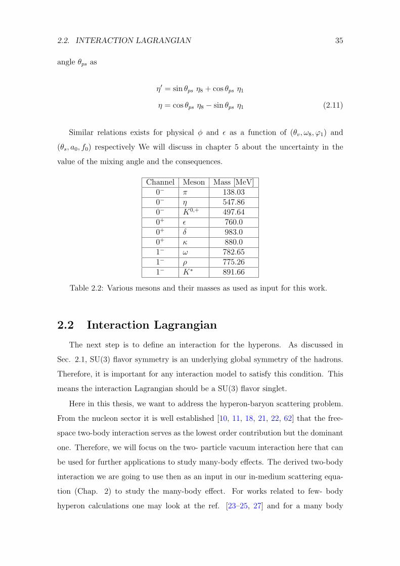
Channel Meson Mass [MeV]0− π 138.030− η 547.860− K0,+ 497.640+ ϵ 760.00+ δ 983.00+ κ 880.01− ω 782.651− ρ 775.261− K∗ 891.66

Table 2.2: Various mesons and their masses as used as input for this work.

2.2 Interaction Lagrangian

The next step is to define an interaction for the hyperons. As discussed in

Sec. 2.1, SU(3) flavor symmetry is an underlying global symmetry of the hadrons.

Therefore, it is important for any interaction model to satisfy this condition. This

means the interaction Lagrangian should be a SU(3) flavor singlet.

Here in this thesis, we want to address the hyperon-baryon scattering problem.

From the nucleon sector it is well established [10, 11, 18, 21, 22, 62] that the free-

space two-body interaction serves as the lowest order contribution but the dominant

one. Therefore, we will focus on the two- particle vacuum interaction here that can

be used for further applications to study many-body effects. The derived two-body

interaction we are going to use then as an input in our in-medium scattering equa-

tion (Chap. 2) to study the many-body effect. For works related to few- body

hyperon calculations one may look at the ref. [23–25, 27] and for a many body


description see ref. [28–32, 32, 34, 35, 38, 39, 41, 43]. However, the two-body in-

teraction is the fundamental baryon-baryon interaction that one should understand

to have a complete knowledge of the baryon interactions. Many of the above ap-

proaches make use of the available two-body interactions as input for their higher

order calculations [36, 37, 40, 41] while others determine the interaction by dir-

ect many-body treatments like mean field theory [38, 39], Brueckner-Hartree-Fock

approximation [42] , Dirac-Bruckner-Hartree-Fock model [32] , density functional

theory [34, 35], quantum Monte Carlo simulations [41, 43]. Nevertheless, due to the

short-range nature of the strong force, two-body interactions are the most dominant

ones and hence can be well sufficient to describe the two-body scattering problem

in a satisfactory manner.

2.2.1 Field Theoretical Description

We want to develop an effective “interacting” Lagrangian consisting of non-zero

two-particle baryon interaction and of course the higher ones which we will neglect

in our work as already discussed earlier.

Let us consider Ψ is the complex baryon field of mass MB. The free field baryon

Lagrangian (LB) containing the kinetic energy and the mass term is given by

LB = iΨBγµ∂µΨB −MBΨBΨB (2.12)

The baryons are “free” here, i. e., moving independently, neither interacting with

each other. Now let the baryons interact with each other however with only one at

a time: not with other fields, that leads to the concept of two-body interaction.

2.2.2 Meson Exchange Forces

For a scalar field, the interaction picture is simple. Baryons being a complex field

and provided the known facts about hyperon is insufficient, we need to tackle this

interaction problem carefully. The first principle of strong interaction, QCD being

complex to handle in hyperon scale, an effective model is a handy tool to fulfil the

gap. Being effective in nature, most of the available nuclear models are mainly


phenomenological. The successful high-precision one-boson-exchange effective nuc-

lear models [10, 11, 62] are trying to circumvent the gap by providing a possible

choice aiming to “reproduce” the well-known nuclear properties making use of the

rich scattering data available for the nucleon sector as well as serving as a good

predicting tool. Following this successful high-precision NN potential models and

their counter parts as an extension including hyperons [46–50], we too will build our

model based on the pioneering idea of Hideki Yukawa [52], quoting his own words:

”The interactions of elementary particles are described by considering a

hypothetical quantum which has the elementary charge and the proper

mass and which obeys Bose’s statistics.[52]”

Figure 2.5: Yukawa Feynman Diagram

Although baryons are no more having the ’elementary particle’ status, still the

meson exchange models are serving as a good approximations compensating the

non-perturbative QCD regime. Yukawa first introduced the idea in terms of a scalar

meson mediator (remember at this time pion was not discovered). The Lagrangian

for this scalar Yukawa Theory is given by

LM =1

2∂µΦ∂

µΦ− 1

2m2Φ2

Lsint = −gBB′sΨB′ΨBΦ

s

LY = LfB + Lf

M + Lsint (2.13)

Here LM represents the meson free field Lagrangian and Lsint is the baryon (B)-


baryon (B)- scalar meson (s)- vertex (2.6) coupling constant “gBB′s”.

B

B

MgBBM

Figure 2.6: Baryon-Baryon-Meson vertex

The Yukawa Lagrangian LY failed to reproduce the ’proper’ nucleon potential

specially in the short ranges (as it is known now that pion is responsible for the

long range part). Physicists tried to overcome the problem by considering multi-

pion exchange models but that too could not solve the problem and the idea of

meson exchange forces were discarded for further use. It was in the 60’s when

the discovery of the other heavy mesons, σ(600), ρ(770), ω(782) etc. opened the

possibility of reviving the Yukawa theory by now including other mesons (bosons)

exchange channels. In the 70’s refined sophisticated ’one-boson-exchange’ theories

were introduced for the nucleon sector by several groups [10, 62]. The Nijmegen

group [11] entered the picture with more precise treatment. Until then a number

of good high-precision NN one-boson-exchange potentials [54, 55, 64] are discovered

and still in use. The main essence of these models is the inclusion of not only scalar

Figure 2.7: One-boson-exchange baryon - baryon -meson vertex

but also pseudo - scalar and vector mesons channels. The new Lagrangian is then

takes the form as given below

LFull = LB + LM + Lint (2.14)

In One–boson–exchange models, the interaction have three different terms, limited

to meson with masses less than 1 GeV, the scalar, the pseudo-scalar, and vector


meson baryon vertices

LMB = Lsint + Lps

int + Lvint (2.15)

Eq. 2.15 defines the interaction Lagrangian used in this thesis. The explicit Lag-

rangian forms of the three interactions are given here

Lpsint : −gBB′psΨB′iγ5ΨBΦ

ps (2.16)

Lsint : +gBB′sΨB′ΨBΦ

s (2.17)

Lvint : −

[gBB′vΨB′γµΨB

(τ · Φv

µ

)− fBB′v

MB +MB′ΨB′σµνΨBF

vµν

](2.18)

Here gBB′ps, gBB′s, and gBB′v are the pseudoscalar, scalar, and vector meson-baryon

coupling constants, τ =∑3

i=1 τi represents the three Pauli matrices, and Fµν is the

field strength tensor given by

Fµν = (∂µ − ∂ν)(τ · Φv

µ

)(2.19)

The above mentioned couplings gave rise to the effective interaction for the baryons.

There exists also gradient coupling of the nucleons by the pseudo-vectors (pv) with

the Lagrangian of form

Lpvint : −fBB′pv

mpv

ΨB′γ5γµΨB∂µΦ

ps (2.20)

The pseudo-scalar and pseudo-vector coupling constants, gBB′ps and fBB′pv, are equi-

valent on-mass-shell condition provided they satisfy the following relation

fBB′pv = gBB′ps

(mps

MB +MB′

)(2.21)

The meson free field Lagrangian is now redefined as

LM =1

2

∑i=ps,s,v

(∂µΦ

µi Φi −m2

ΦiΦ2

i

)− 1

2

∑M=V

(1

2F (M)2 −m2

MV 2κ

)(2.22)


2.3 Effective Model Parameters

The effective interactions defined in Eq. 2.16, 2.18, 2.17 are characterized by

three factors:

1. The value and sign of the coupling strength of the interaction ver-

tex (g):

+ sign : attractive interaction ( e.g: scalar)

- sign : repulsive interaction (e.g: pseudo-scalar, vector, pseudo-vector)

2. Mass of the meson (m): Determines the range of baryon-baryon interac-

tion the meson is responsible for.

3. Type of meson (JP): Determines the Lorentz structure of the vertex and

hence the Lagrangian as shown in Eq. 2.16, 2.18, 2.17.

Among these three, the critical ones are are the first two. In the following, we discuss

these two factors in detail.

2.3.1 Meson Masses

Pure SU(3) symmetry demand the multiplets to be mass degenerate. However as

already found by in the early decades of quark model discovery [12, 14] that this

is not the case and the physical mass values are different. These mass difference is

coming out of the explicit symmetry breaking due to strange quark (s) being slightly

heavier than the up (u) and down (d) ones. The observed particles are called as

the ’physical’ ones. Therefore, for any SU(3) model to be realistic, one must study

these physical particles. We, in this work, incorporate this breaking by using the

physical mass values of the particles.

In Table 2.3 the physical mesons are listed with their spin (J), isospin (I), mass

reported by Particle Data Group [16], and the full width of the particles in the

complex plane. From the table it can be noticed that except for the strange K−,+

pseudo-scalar meson, which has a two close bump structure (see Fig. 2.10), the

pseudo-scalar and vector mesons are easy to identify as particles due to sharp peak in

2.3. EFFECTIVE MODEL PARAMETERS 41

Figure 2.8: f0(500) scalar meson pole positions in complex energy plane. Figuretaken from [126]

Meson Spin (JP ) Isospin (IG) Mass [MeV] Full Width [MeV]π± 0− 1− 139.57018 0π0 0− 1− 134.97660 0η 0− 0+ 547.86000 .00131η′ 0− 0+ 957.78000 0.198

K0,+ 0− 12

497.64000 –ϵ 0+ 0+ 760.00000 400-700

a0 (δ) 0+ 1− 983.00000 50-100κ 0+ 1

2880.00000 547

ω 1− 0− 782.65000 8.49ρ 1− 1+ 775.26000 149.1K∗ 1− 1

2891.66000 –

Table 2.3: Meson masses

the complex energy plane, but for scalar mesons it is an ongoing problem, thus arising

the so-called ’meson puzzle.’ . In fact, there is long debate among different groups

Type Meson Resonances as in [16] TotalPseudo-scalars η η(1295),η(1405),η(1475),η(1760),η(2225) 5

Scalar f0 f0 (500),f0 (980),f0 (1370),f0 (1500), 9f0 (1710),f0 (2020),f0 (2100),f0 (2200),f0 (2330)

Scalar a0 a0(980),a0 (1450) 2Vector ω ω(782),ω(1420),ω(1650) 3

Table 2.4: Different resonances available for mesons

whether the respective resonances for the scalar mesons are actually representing a


Κ-

Κ

-0

Κ0

f0H500La0- a0

0a0+

Κ+

f0H980L

Figure 2.9: Scalar meson octet.

single particle (read scalar meson) or resonances between two other light particles.

This discrepancy has lead many physicists to discard the scalar meson sector and

approaching the problem as two or multi-particle resonances, for example, the latest

Julich hyperon model [48] considers the scalar-isoscalar σ meson interactions as ππ.

Moreover, a look at the PDG listing of particles, one can find a long list of

particles with same nomenclature but with different resonances or pole positions,

for all types of mesons, making it difficult to position the particle in the particle

plane. Particularly for the scalar mesons the determination of the width is very

model dependent. For example the Fig. 2.8 one can see various pole positions of

the f0(500) scalar meson as reported in [16]. The mesons used in this thesis and

their corresponding PDG listed particle identifiers are reported in Table. 2.5. An

scalar-isoscalar meson ϵ (or σ) is used to provide intermediate- range interaction as

done by [11, 49, 50, 62], to make the model realistic. For the mass we choose a value

of 760 MeV, following ESC group [49].

2.3.2 Coupling Constants

In order to use the effective Lagrangian (Eq. 2.15), the required input is the correct

coupling strengths of the meson-baryon vertices. The more precise the values are,

the larger the predictive power of the model will be. There are few possible way

outs for determining the coupling:


Figure 2.10: K−,+ pseudo-scalar meson pole positions in complex energy plane. Thisfigure is taken from [16].

Meson PDG2012 listed particle Mass [MeV]identifier

π± π± 139.57018π0 π0 134.9766η η 547.86

K0,+ K0,+ 497.64ϵ f0(500) 760.0a0 a0(980) 983.0κ K∗

0(800) 880.0ω ω(782) 782.65ρ ρ(770) 775.26K∗ K∗(892) 891.66

Table 2.5: Meson used in this model listed according to the PDG identifiers [16].


Phenomenological method: treating them as parameters and fix the values

then by fit to approximately chosen experimental values. This is how the

nucleon meson-nucleon coupling constants are fixed [10, 11, 54, 62, 64]

Theoretical method: Fix the values by theory. Usually by symmetry or other

relevant physical constraints the theory demands. In the future, results from

lattice QCD (LQCD) could be used.

The ’hybrid’ method: A mixture of all the above, e.g., use theoretical relations

to eliminates the number of free parameters and determine only a subset by

phenomenology.

As far as hyperons are concerned, phenomenology is ruled out due to few data

points compared to the number of channels. Therefore, the usual practice here is to

fix the values by theory, here it is SU(3). However, since SU(3) is not exact, many

groups use the third approach, for example the various models of Nijmegen groups

differ by the choice of coupling strengths [49, 50] as well as for the Julich model

also have varied the coupling strength values in their different versions [46–48]. The

one-boson-exchange potential will be discussed in more detail in the next chapter.

Here in this thesis, we will constraint ourselves to SU(3) symmetry. However, we

will use the physical particle masses to make the model realistic and allowing this

explicit breaking. Our aim is to have a qualitative understanding of the baryon-

baryon octet interactions. One of our major application of the free space interaction

is to find the medium effect on it. For this reason, we, at this moment, do not

indulge on the complexities involved in countering the breaking involved. In the

next section, we discuss how the coupling constants are determined in our case

using SU(3) symmetry.

2.3.3 Octet-Octet and Octet-Singlet Interaction

We have already discussed in Sec. 3.1 that baryons are observed to have the octet

structure represented as 8B (Fig. 2.1). SU(3) symmetry demands the Lagrangian to

be SU(3) invariant,i.e., SU(3) scalar. This means all our interaction terms defined

in the previous section (Eq. 2.16-2.18) should be SU(3) singlet. We have already


defined our interaction vertices as baryon-baryon-meson (BB’M) one. In terms of

group theory, this means we need to construct SU(3) scalar with the meson nonets

(8M,1M) and the baryon current 8B⊗8B. This has been worked out completely by

J.J. de Swart [56] in 1965. In the following, we describe the method of determining

g’s from SU(3) considerations.

The baryon current yields the following six representations

8B ⊗ 8B = 27⊕ 10⊕ 10∗ ⊕ 81 ⊕ 82 ⊕ 1 (2.23)

81 and 82 corresponds two distinct octet representations of same dimension. 81

is symmetric under the exchange of the coupled basis elements, while 82 is the

antisymmetric under same condition. The reason why these two are named distinctly

is that these results in two different types of coupling:

D- coupling : Results from the coupling between symmetric baryon multiplet

81 with meson octet 8M with strength gD

F- coupling :Results from the coupling between anti-symmetric baryon octet

82 with meson octet 8M with strength gF

There are now two ways in which now one can construct a SU(3) scalar out of a

baryon–baryon–meson coupling, namely

1. Octet-octet coupling : 8B ⊗ 8B ⊗ 8M

2. Octet-singlet coupling: 8B ⊗ 8B ⊗ 1M

2.3.4 SUf(3) Baryon-Baryon-Meson vertices

In eqs. 2.4-2.7 the SU(3) invariant traceless baryon and octet matrices has been

shown. The available SU(3) invariant combinations using these matrices are the

following

Tr (BMB), Tr (BBM), Tr (BB) Tr (M)


The definition of the anti-symmetric (F), symmetric (D) , and singlet(S) SU(3)

scalars are then

[BBM]F = Tr (BMB)− Tr (BBM)

= Tr (BM8B)− Tr (BBM8)

= Tr ([B,B]M8) (2.24)

[BBM]D = Tr (BMB)− Tr (BBM)− 2

3Tr (BB) Tr (M)

= Tr (BM8B) + Tr (BBM8)

= Tr (B,B

M8) (2.25)

[BBM]S = Tr (BB) Tr (M)

= Tr (BB) Tr (M1) (2.26)

Here [B,B] represents the B,B commutator and B,B is the corresponding anti-

commutator. Now we can re-define our same interaction Lagrangian 2.15 in terms

of these SU(3) flavor invariants. The SU(3) interaction Lagrangian is a linear com-

binations of the F,D, and S scalars defined above

LSU(3)MB = −g8

√2α[BBM8

]F+ (1− α)

[BBM8

]D

− gS

√1

3

[BBM1

]S

(2.27)

Here a new constant α, known as the FF+D

-ratio, is introduced with the definition

α =gF

gF + gD(2.28)

where g8 and g1 are the octet and singlet coupling constant respectively. Apart

from SU(3), another important feature of the Lagrangian is isospin symmetry. The

Lagrangian should also be isospin invariant. Let us define the following baryon (N,Λ,

Σ, Ξ) and meson (K, Kc, π) isospin multiplets

N =

np

,Λ = Λ, Σ =

Σ+

Σ0

Σ−

,Ξ =

Ξ0

Ξ−

(2.29)


π =

π+

π0

π−

, K =

K+

K0

, Kc =

K0

−K−

(2.30)

As has been worked out by [56], the most general isospin invariant meson octet

Lagrangian (shown for π as an example) is of the following form

mπL8MB = −gNNπ(NΓτN)·π + igΣΣπ(Σ×ΓΣ)·π

− gΛΣπ(ΛΓΣ + ΣΓΛ)·π − gΞΞπ(ΞΓτΞ)·π

− gΛNK

[(NΓK)Λ + ΛΓ(KN)

]− gΞΛK

[(ΞΓKc)Λ + ΛΓ(KcΞ)

]− gΣNK

[Σ· Γ(KτN) + (NΓτK)·Σ

]− gΞΣK

[Σ·Γ(KcτΞ) + (ΞΓτKc)·Σ

]− gNNη8(NΓN)η8 − gΛΛη8(ΛΓΛ)η8

− gΣΣη8(Σ·ΓΣ)η8 − gΞΞη8(ΞΓΞ)η8. (2.31)

with the singlet interaction of the form

mπL1MB =

[gNNη1(NN) + gΛΛη1(ΛΛ) + gΣΣη1(Σ · Σ) + gΞΞη1(ΞΞ)

]η1 (2.32)

We follow the de Swart [56] phase convention that defines the inner product of the

isovector Σ- baryon and π-meson in the following form

Σ·π = Σ+π− + Σ0π0 + Σ−π+ (2.33)

gNNπ = gps8 gNNη8 =1√3(4αps − 1)gps8 gΛNK = − 1√

3(1 + 2αps)g

ps8

gΞΞπ = −(1− 2αps)gps8 gΞΞη8 = − 1√

3(1 + 2αps)g

ps8 gΞΛK = 1√

3(4αps − 1)gps8

gΛΣπ = 2√3(1− αps)g

ps8 gΣΣη8 =

2√3(1− αps)g

ps8 gΣNK = (1− 2αps)g

ps8

gΣΣπ = 2αpsgps8 gΛΛη8 = − 2√

3(1− αps)g

ps8 gΞΣK = −gps8

Table 2.6: Pseudo-scalar meson-baryon coupling constants


Incorporating the SU(3) invariance conditions to the isospin invariance, the

pseudoscalar meson coupling constants need to satisfy the following relations (Tab.

2.6). Similar relations for the vector and scalar mesons are given in Tab. 2.3.5. The

singlet mesons couples universally with baryons (Table 3.4).

ps gNNη1 = gΛΛη1 = gΣΣη1 = gΞΞη1 = gps1v gNNϕ = gΛΛϕ = gΣΣϕ = gΞΞϕ = gv1s gNNσ1 = gΛΛσ1 = gΣΣσ1 = gΞΞσ1 = gs1

Table 2.7: Singlet meson-baryon coupling constants

2.3.5 Free Parameters

From the relations above, it is clear that three parameters are governing the coupling

of a particular type of meson (ps,s,v) with baryons

1. the octet coupling strength (g8)

2. the FF+D

-ratio (α)

3. the singlet coupling strength (g1)

So considering three types of mesons we have in total 9 parameters. However, there

is one extra parameter that need to be taken into account to incorporate the octet-

singlet mixing: the mixing angle (θ) already defined in eq. 2.11. In addition, there

is the standard set of OBE model parameters containing meson masses and form

factor parameters. These will add to the count and in total our parameters are

summarized in Table. 2.10.

gNNρ = gv8 gNNω8 =1√3(4αv − 1)gv8 gΛNK∗ = − 1√

3(1 + 2αv)g

v8

gΞΞρ = −(1− 2αv)gv8 gΞΞω8 = − 1√

3(1 + 2αv)g

v8 gΞΛK∗ = 1√

3(4αv − 1)gv8

gΛΣρ =2√3(1− αv)g

v8 gΣΣω8 =

2√3(1− αv)g

v8 gΣNK∗ = (1− 2αv)g

v8

gΣΣρ = 2αvgv8 gΛΛωv

8= − 2√

3(1− αv)g

v8 gΞΣK∗ = −gv8

Table 2.8: Vector meson-baryon coupling constants

There is an additional parameter too, namely the form factor, that needs to be

multiplied with each BB′M vertex to regularize the high-momentum behavior. We

will discuss about this later in detail. The model we will use is a low-energy effective


gNNa0 = gs8 gNNϵ =1√3(4αs − 1)gs8 gΛNκ = − 1√

3(1 + 2αs)g

s8

gΞΞa0 = −(1− 2αs)gs8 gΞΞϵ = − 1√

3(1 + 2αs)g

s8 gΞΛκ = 1√

3(4αs − 1)gs8

gΛΣa0 =2√3(1− αs)g

s8 gΣΣϵ =

2√3(1− αs)g

s8 gΣNκ = (1− 2αs)g

s8

gΣΣa0 = 2αsgs8 gΛΛϵ = − 2√

3(1− α)gs8 gΞΣκ = −gs8

Table 2.9: Scalar meson-baryon coupling constants

theory. Therefore, there is a certain limit up to which the model will give realistic

result. This is taken into account by the form factor. In higher energy regime, many

other degrees of freedom will enter the system which is not treated in our model.

Here we use a dipole form factor having the following form

F2(k) =

(Λ2

c −m2

Λ2c + k2

)2

(2.34)

Λc is called the cut-off. Here k is the relative momenta between the initial and

final baryon. ”m” is the mass of the meson involved as a force carrier. Λc has the

dimension of mass usually chosen as 500- 600 MeV higher than the meson. The value

of Λc fixes the higher momentum domain of the calculation. For massive mesons

(σ), Λc is much higher than lighter ones (π). As it is found out, the value of Λc also

effects the behavior of the model [46, 47, 49, 50]. The Nijmegen-Tokyo group [50]

uses each vertex cut-off as a parameter. In our case, we have fixed the value of the

cut-off for the whole meson octet that reduced the number of parameter significantly.

Table 1.8 summarizes the parameters used in this thesis. In Table. 2.10 the free

parameters of the model are listed, total 15 in number. These parameters are fixed

by preferably by fitting to the scattering data available However, due to a limited

number of data set that is insufficient to fix the parameters with desired accuracy,

some of the parameters are fixed from theoretical aspect. The details of the fitting

procedure will be discussed in Chapter 5. We will keep updating this parameter list

Meson Parameters Total Parameter(Meson Octet)

pseudo-scalar gps8 , gps1 , αps,Λ

psc , θps 5

vector gv8, gv1 , αv, θv,Λ

vc 5

scalar gs8, gs1, αs, θs,Λ

sc 5

Total Model Parameter: 15

Table 2.10: Parameters of the model.


as we start discussing the results to minimize the parameter even more by putting

constant values to the less sensitive ones.

2.4 Comparison with Contemporary Models

There exists few more hyperon models based on OBE, namely the Julich models,

Extended-soft-core (ESC) models (known as Nijmegen models too). The basic phys-

ics followed by these two and the one used in this work, are same. However, there

exists various significant differences in the treatment of the of actual problem e.g.,

the choice of parameters, extent of SU(3) symmetry used, scalar-isoscalar mesons

taken into account, responsible for the intermediate range attraction, form factor

etc. In the following, these differences has been pointed out.

1. Mesons: The first difference between the other two and our one is the number

of mesons being included. We are trying to follow SU(3) as much as we can,

including all the nonet mesons, except the ϕ one, which did not found to

have much effect on the hyperon sector [46, 47]. Moreover, we do not include

higher lying mesons except the lower ones. We do not have any other extra

mesons in our models. On the other hand, the ESC-models although usually

use all the SU(3) mesons yet they have a fictitious particle ’pomeron’ in their

model. Esc group also considers all the massive mesons in their models. In

total the number of meson channels they have are way higher than ours. Con-

cerning the Julich models (no more in continuation), there are three versions

available: 1989, 1994, and 2005 one. The first two being much similar, have

octet mesons. Our model is quite similar to the early versions of Julich models

in this particular point. The latest Julich one discarded the e scalar-isoscalar

(σ) and the vector-isovector (ρ) completely and used ππ and KK exchange

channels instead.

2. Boson-exchange vertices: The other important factor is the diagrams taken

into account of the potential involved. We have only considered One–boson–

exchange diagrams. Both ESC and Julich groups have in some of their versions

two-meson (usually ps) exchange diagrams and sometimes delta resonances

2.4. COMPARISON WITH CONTEMPORARY MODELS 51

[47]. The very recent ESC model includes multi-pomeron channels.

3. Parameters: We have minimized the parameters by fixing them for a type

of octet and using SU(3). Where as Julich models have all their vertices as

parameters for the all of their version. For ESC one, the parameter choice is

similar to ours but with a major difference that they usually make different

versions depending on the parameter values [50]. There fore, the parameters

are not actually fixed.

4. Cut-off : The choice of form factor is also different. Ours is similar to Julich

one where as ESC group uses a Gaussian type form-factor.

5. Momentum or Co-ordinate Space?: We will write the potential and solve

the scattering equation, to be discussed in next chapter, in momentum space

similar to Julich model. On the other hand, the Nijmegen group prefers the

co-ordinate space version and solve the equation in r-space. This is just a

matter of choice in which one is comfortable to deal the problem as the final

physics should be independent of the choice of the solving procedure.

6. Fitting Procedure: Both the Julich and ESC models starts from the nucleon

sector. In order to have a good fit with the nucleon data, the SU(3) values are

already modified specially for the vector mesons. On the other hand, in order

to study the SU(3) symmetry in close attention, the nucleon values are not

fitted by our parameters. On the contrary, in this work, the reverse approach

is followed. We first fitted the hyperon sector and then used the parameters

to the nucleon sector.

7. SU(3) Flavor Octet Interaction: As already mentioned, the basic interest

of revising the OBE models is to study the SU(3) symmetry range of applic-

ability in terms of octet interaction. We are allowing the breaking only via

physical particle masses. The coupling constant relations are not disturbed.

As discussed in the previous point, fitting the nucleon sector, the SU(3) is

already broken by some extent for both the other models. Also the earlier

Julich model considered SU(6) symmetry and the latest one is more on the


phenomenological side. The ESC and Nijmegen ones are using SU(3) sym-

metry. However, they use explicit breaking terms and mesons outside the

octet, that also does not preserve the SU(3).

2.5 Summary of the model

In the following a list is given with the key points of the One–boson–exchange

model based on SU(3) symmetry used in this thesis

1. This is an effective model with boson-exchange effective interactions.

2. The bosons (mesons) used belong to the SU(3) meson octet and the respective

singlets

Pseudo-scalar : π, η, η′, K0

Vector : ρ, ω,K∗

Scalar : a0, ϵ, κ, ϵ′

3. Effective meson-baryon coupling constants are determined using SU(3) rela-

tions.

4. Physical particle masses according to PDG [16] are used to account for explicit

symmetry breaking.

5. A dipole form factor is multi-plied to each BB′M vertex to control divergence.

6. The free parameters are fixed by fitting to scattering data.

Chapter 3Scattering Theory and Formalism

“Physicists have come to realize that

mathematics, when used with sufficient

care, is a proven pathway to truth.”

Brian Greene

Now since the model is defined in Chap. 2, the next step is to use it in real

systems. Scattering is an important experimental tool for quantum systems. For

microscopic physics, most of our knowledge is indebted to scattering experiments.

For hyperon-baryon interactions, scattering is a powerful technique to gain under-

standing about the interaction. Here the test of the model is to be able to reproduce

scattering data set when used as theoretical input. Therefore, it is worthwhile to

spend few pages on describing the two-body scattering problem.

In Section 1, basic kinematics for two body scattering is described briefly. Section

2 and 3 are devoted on describing theoretical descriptions of scattering processes by

describing Bethe-Salpeter and Lippmann-Schwinger equations. In Section 4, isospin

basis formalism is discussed for the scattering channels in connection with isospin

symmetry conservation. A special characteristics of the hyperon included baryon

scattering channels, the coupled channel formalism is the topic for discussion in

Section 5. The formation of the OBE potential amplitudes relevant to our model

has been discussed in detail in Section 6.

53

54 CHAPTER 3. SCATTERING THEORY AND FORMALISM

3.1 Kinematics

The kinematics of a scattering process is described largely by the energy and

momentum conservation laws without depending on the detailed dynamics involved

in the process.

A scattering is called elastic when outgoing particles are identical as the incoming

ones,

A+B → A+B

In case of elastic collision, the particles only exchange kinetic energy and momentum

between themselves. On the other hand, a collision is called inelastic when at least

one of the particle changes its internal state after collision.

A+B → A∗ +B

Here A∗ is a excited state of particle A. A scattering can also be a reaction where

A+B → C +D + E...

C, D, E are the reaction products, which are not identical to the incoming particles.

In this thesis we will restrict ourselves to the simplest case of two body scattering.

A+B → C +D

3.1.1 Relativistic kinematics of Two-particle Scattering

For a particle having energy E and three-momentum p, the relativistic four-momentum

P is defined as

P µ = (P 0, p) = (E

c, p) (3.1)

The relation between relativistic energy (E) and three-momentum is given by

E2 = p2c2 +m2c4 (3.2)

The four-momentum Pi of any particle i satisfies the relation (in natural unit c = 1,

~ = 1 )

P µi P

iµ = E2

i − p2i = m2i (3.3)

3.1. KINEMATICS 55

A

C

D

pA

pC

pD

Θ

ΦB

Figure 3.1: Two body scattering in laboratory frame

In this thesis we are interested in hyperon -baryon two body scattering reactions.

A+B → C +D

where particle A of mass m1 collides with particle B of mass m2.

Usually in particle physics experiments, one particle remains at rest, known as

the target, and the other one is made to collide with the target (called projectile

or incident or beam particle). The reference frame in which the target particle is

at rest is known as the laboratory (lab) frame as shown in Fig. 3.1. The center-of

mass frame (CM) is the one in which total three momentum of the reaction is zero

as in Fig. 3.2.

pA pB

pC

pD

Figure 3.2: Two body scattering in center-of-mass (CM) frame

The usual convention is to consider the direction of beam particles along positive

z axis. Let us consider the beam particle A has momentum plab in the laboratory

(lab) frame along z axis. The outgoing particle C (mass m3) and D (mass m4 ) are

detected in the lab frame at an angle θ having momentum p3 and at angle ϕwith

momentum p4 respectively with respect to the direction of travel of the projectile


p1 [Fig. 3.1]. Consider E1, E2, E3 and E4 are the energy of the particles A, B, C

and D respectively in lab frame. Since the target is at rest in laboratory frame, we

have,

p2 = 0 (3.4)

Now let us consider P1, P2, P3, P4 being the four-momenta of the particles A, B,

C, and D respectively in the reaction under investigation. The total four-momentum

is always conserved in any collision in any reference frame, hence

P1 + P2 = P3 + P4

Now in case of the target and beam scattering,i.e, for particles A and B in Fig.

3.1, we have, in lab frame,

P1 =

E1(plab)

plab

, P2 =

E1(0)

0

In case of CM frame, considering the corresponding CM variables as asterisked

(Pi = P ∗i ), we have,

P ∗1 = −P ∗

2 , P∗3 = −P ∗

3 (3.5)

In relativity, the dot product of two four-vectors is a Lorenz invariant quantity

and usually known as Lorenz scalar. Out of the possible invariant Lorenz scalars,

e.g, P1.P1, P1.P2,P3.P4 etc., due to the constraints, only two are left as variables.

Recalling the definitions of the Mandelstam variables,

s = (P1 + P2)2 = (P3 + P4)

2 (3.6)

t = (P1 − P3)2 = (P2 − P4)

2 (3.7)

u = (P1 − P4)2 = (P3 − P2)

2 (3.8)

we see they serve as a possible Lorenz scalar choice. It follows from these definitions

that s- Mandelstam variable is square of the total CM energy where t is the four-

momentum transfer squared between 1 and 3. It is straight forward to see that the

3.2. SCATTERING EQUATIONS 57

Mandelstam variables also satisfy

s+ t+ u = m21 +m2

2 +m23 +m2

4 = constant (3.9)

Some useful formulas concerning scattering between CM and lab frame are summar-

ized below:

plab =

√(s−m2

1 −m22)

2 − 4m21m

22

4s(3.10)

In terms of plab, the s mandelstam variable, the total energy squared of the system

is given by

s = m21 +m2

2 + 2m2

√p2lab +m2

1. (3.11)

3.2 Scattering Equations

The quantity we are interested in this kind of problems is the scattering amp-

litude. The time scale over which the particles interact are extremely short. Con-

sidering the time of interaction as t, then −∞ ≪ t≪ ∞. For times long before and

after the interaction, the incident particles are free. These two regions are known as

the two asymptotic regions, one in distant past (tin) and one in distant future (tout).

The scattering operator is defined mathematically as

S | Ψi >=| Ψf > (3.12)

Scattering matrix S measures the transition probability of state ψi to ψf .

Sfi ≡< ψf | S | ψi > (3.13)

3.2.1 Bethe-Salpeter Equation

In this thesis, we focus on hyperon (Y) -baryon (B) scattering problems.

B1(q1) + B2(q2) → B3(q3) + B4(q4)


Particle physics scattering problems needs to be dealt not only from quantum mech-

anical but relativistic point of view. Therefore one can not start form the non-

relativistic Schroedinger equation or it’s counterpart Lippmann-Schwinger equation

being a non-relativistic scattering equation. As far as nuclear physics is concerned,

Bethe-Salpeter equation is the answer to the problem. Bethe-Salpeter equation

(BSE) for a two-particle relativistic scattering in momentum space can be represen-

ted as [57]

T (q′, q | E) = V(q′, q | E) +∫d4k V(q′, k | E) G(k | E) T (k, q | E) (3.14)

where q′, q, and k are final, initial, and intermediate relative four-momenta of the

particles, respectively, E is implying constant energy, T is the total invariant two-

particle scattering amplitude, V is the sum of all possible two-particle connected

irreducible diagrams, and G is the relativistic two-particle free propagator, the Green

function, which is represented in momentum space as

G12(q1, q2) = G1(q1) G2(q2) =

(1

γµq1µ −M1 + iϵ

)(1

γµq2µ −M2 + iϵ

)(3.15)

where M1 and M2 are the masses of particle 1 and 2. The diagrammatic repres-

entation of BSE is shown in Fig. 3.3. The more convenient way is to represent

+=T V V G T

Figure 3.3: Diagrammatic representation of Bethe-Salpeter Equation

Bethe–Salpeter equation in the operator notation as following:

T = V + V G T = V + V G V + V G V G V + ... (3.16)

3.2. SCATTERING EQUATIONS 59

This is a self-consistent equation. The first term V can be interpreted as a relativ-

istic potential. The possible Feynman diagrams contained in V is shown in Fig.

[3.4]. Considering only the highest (first term ) order contribution to the kernel

+ + +V=

Figure 3.4: Irreducible Kernel V of Bethe-Salpeter Equation. The solid line represents the baryonand the dashed line is for meson.

V , represented as V0, neglecting the crossed order contributions, then scattering

amplitude T get the form as shown if Fig. 3.6. It is clear from Fig. 3.6 that

V H0L=

Figure 3.5: Highest order term of V of Bethe–Salpeter equations (Eq. 3.14)

various contributing terms to T looks like a ladder. Thus came the name ”ladder

approximation” for this truncation scheme. In this thesis, the one-boson exchange

potential (OBE) used corresponds to the term V(0) in Fig. 3.5. Here the dotted line

represents the ’meson’ acting as the force mediator between the baryons that are

trying to interact with each other. Within the ladder approximation scheme, the

crossed and other higher order terms are being neglected. The main reason behind

this as a starting point are the facts that, first of all, a basic approach in physics is

to start from the simplest interaction first then gradually adding the complexities.

Following the same strategy, we for this time being, focused on V(0) only. Secondly,


+ + + ...T=

Figure 3.6: Bethe-Salpeter Scattering amplitude in ladder approximation

the order of magnitude of the higher order terms is much less as compared to the

first one for this kind of two-body scattering problem as found already by various

groups [11, 46, 49, 55, 62]. Whether this approximation is well enough or a crude

one, that can be clear after the theoretical calculations are compared with the avail-

able date set. One important point to be worth mentioned here is that the way our

model is build, if it is found at later stage that the higher order or crossed terms are

unavoidable, they can be added conveniently to the scheme.

3.2.2 Lippmann-Schwinger Equation

The main difficulty with BSE is its 4-dimensional integral structure, which makes it

difficult to solve. The usual way of making it workable is to reduce it to an equivalent

3-dimensional equation not affecting the covariant and relativistic elastic unitarity.

The reduction scheme is not however unique. The reduction is done by considering

an unknown operator U for the kernel that satisfies an analogous Bethe–Salpeter

type equation with U defined as Eq. (3.17)

T = U + UGT

U = V + V(G − g)U (3.17)

Here g is a three-dimensional propagator. By method of insertion then it is straight-

forward to see that T is indeed the Bethe–Salpeter amplitude. For Eqs. (3.14) and

(3.17) to be equivalent, g needs to be simple, (G-g) needs to small, and G and g

should have the same elastic unitarity cut in the physical region. Here in this thesis,

the Blancenbekler-Sugar operator(BbS) [58] has been used as g for the reduction.

3.3. ISOSPIN BASIS 61

BbS reduction converts BSE to the following 3-D Lippmann-Schwinger type non-

relativistic equation

T (q′,q | E) = V (q′,q | E) +∫d3k V (q′,k | E) G12 T (k,q | E) (3.18)

Eq. 3.18 has formally the same form as BSE, an essential difference is that the integ-

ration is now over three dimension and T and V are defined now under the ’minimal

relativity’ condition, refers to considering the relativistic kinematics properly, taking

only the positive-energy Dirac spinors into account. A detailed calculation of the

derivation can be found in [59]. G is the non-relativistic two-particle propagator

given by

G12 =2µ12

q2 − k2 + iϵ(3.19)

with µ12 being the reduced mass of the two interacting baryons

µ12 =M1M2

M1 +M2

(3.20)

By using Eq. 3.18 the full scattering matrix T is obtained by iterating over the

term V, now the one-boson-exchange potential. We need to solve this equation to

get various information about the hyperon-baryon scattering using out interaction.

Before discussing about the numerical solution strategy, it is important to have

a knowledge about the scattering channels. In next section, octet baryon-baryon

channels are discussed.

3.3 Isospin Basis

In Chap. 2, we have discussed about the JP = 12

+baryon octet that is our

prime focus in this work. In Table 3.1 these baryons are listed with their observed

spin, parity, charge and the quark content. It has been already discussed that SU(2)

isospin symmetry is a subgroup of SU(3) flavor symmetry. Therefore, the effective

interaction should be an isospin conserving one. In Eq. 2.31 the interaction is shown

in one -way of isospin symmetry preserving manner using the baryon (N, Λ, Σ, Ξ)

and meson (π, K, Kc) isospin multiplets defined via Eqs. 2.29 and 2.30. Considering


Baryon Component Isospin (I) Isospin (I3) Charge (Q)

n udd 12

12

−0

p uud 12

12

++1

Λ uds 0 0 0Σ+ uus 1 1+ +1Σ− dds 1 1− -1Σ0 uds 1 0 0

Ξ− dss 12

12

−-1

Ξ0 uss 12

12

+0

Table 3.1: JP = 12

+Baryons with their quark component, isospin, third component of isospin

(I3), and charge (Q)

SUf (3) as an exact internal symmetry, the resonant particles must belong to the irre-

ducible representations of SUf (3) introduced in the previous Chapter. On the other

hand, for isospin to be a full symmetry, the particles in an isospin multiplet must

have the same mass-spin-parity (space-time properties) of the one-particle states.

A look on the baryon isospin multiplets (see Table. 3.2) shows that the individual

particles of the multiplets differ by electric charge having same spin and almost same

mass. This mass-splitting is due to an interaction that can distinguish the particles

by some property, here as we can see by charge, hence it is the electromagnetic

interaction. Therefore, if we neglect the electromagnetic interaction, the space-time

properties of all particles of a multiplet are identical to each other. As for example

the isospin multiplet of N, Λ, Σ, and Ξ baryon has one or more members with same

spin, parity and slightly different masses as shown in Table. 3.2. The mesons also

have this isospin symmetry inbuilt (see Table. 3.3). The multiplicity of the mul-

tiplets refer to the dimension of the irreducible representation we have discussed in

previous chapter. The SU(3) isospin multiplets discussed about are consist of one-

particle states. Our aim in this thesis is to study the hyperon-baryon interaction in

connection with the two-body scattering. For that we need to understand the isospin

transformations of the two baryon channels. Multi-particle states transform accord-

ing to the direct product of the single-particle states representation that has been

used earlier in Chapter 2 to derive the baryon and meson SU(3) traceless matrices

(Eq. 2.4-2.7). Neglecting the electromagnetic and weak interaction and considering

the isospin symmetry to be exact, the scattering matrix S and hence the T-matrix

3.3. ISOSPIN BASIS 63

Baryon Strangeness(S) Multiplet Mass Spin (J) Parity (P)

N 0

(np

) (939.57938.27

)12

+

Λ -1 Λ 1115.683 12

+

Σ -1

Σ+

Σ0

Σ−

1189.371192.641197.45

12

+

Ξ -2

(Ξ0

Ξ−

) (1314.861321.71

)12

+

Table 3.2: Baryon isospin multiplets with their space-time properties*.

Meson Multiplet Mass Spin Parity

π

π+

π0

π−

139.57134.97139.57

0 -

η η 547.862 0 -

K

(K+

K0

) (493.677493.677

)0 -

Table 3.3: Meson isospin multiplets with their space-time properties.

have diagonal form in isospin basis with respect to isospin I leaving the dynamics of

the system unchanged for isospin rotations. This leaves total isospin I as conserved

therefore we have

[S, I] = 0, [T, I] = 0 (3.21)

This implies that the isospin can form a basis for the scattering problem. Corres-

pondingly the T-matrix elements can be written now as an expansion in terms of

isospin scattering amplitudes T (I), scattering amplitude T for isospin I, an expan-

sion in the isospin basis. For our two baryon scattering process B1B2 → B3B4 the

expansion is then given by

⟨B3B4|T |B1B2⟩ =∑I

T (I)Ω(I;B1, B2;B3, B4). (3.22)

The element Ω(I;B1, B2;B3, B4) calculates the projection of T on a state of isospin

I. By construction here each scattering amplitude T (I) is isospin invariant. For-

mulating now the mentioned isospin expansion scheme to the octet SU(3) baryon

channels, say B8B8 channels can be written in isospin basis. In Table 3.3 the B8B8


baryon channels have been tabulated accordingly in the isospin basis, defined in this

case as channels grouped according to total strangeness (S) and isospin (I).

I = 0 I = 12

I=1 I = 32

I=2

S=0 NN NN

S=-1 ΛN , ΣN ΣN

S=-2 ΛΛ, ΞN , ΣΣ ΞN , ΣΛ , ΣΣ ΣΣ

S=-3 ΞΛ, ΞΣ ΞΣ

S=-4 ΞΞ ΞΞ

Table 3.4: Baryon-baryon channels in isopin basis

3.4 Coupled Channel Formalism

One new and interesting feature of the two baryon scattering problem appears

when strangeness channels are included, the so called ’coupled channel’ behavior.

The channels with only single entry is called as uncoupled. For example the ΣN , I =

32channel is a pure isospin-3

2channel. Isospin conservation prohibits the coupling

of this channel with any other. See in Table 3.3 that for channels S ≤ −1, there are

few isospin channels having more than one sub-channels. For example, consider the

S = −1, I = 12subset, it has two BB channels : ΛN and ΣN as the elements. This

means that these two channels together span the S = −1, I = 12subset. However,

due to the mass difference between the ’physical particles’, the massive particle

channel ΣN opens has a higher threshold energy

Ethreshold =√s =MΣ +MN . (3.23)

Hence, ΣN channel will open at higher input momenta than the other member ΛN

since MΣ −MΛ > 0 (see Table 3.3). In particular for this case the ΣN threshold

pointing to the laboratory momenta at which the channel opens up is

pthlab(ΛN → ΣN) = 643.8 MeV/c. (3.24)

In Fig. 3.7 total energy (√s) of S = −1, I = 1

2channels (orange: ΛN , blue(solid):

3.4. COUPLED CHANNEL FORMALISM 65

1800 1900 2000 2100 2200 2300 2400 25000

200

400

600

800

s @MeVD

q BB@M

eVD

Figure 3.7: Center-of-mass momentum vs energy plot of NN (blue dashed), ΛN (orange) andΣN (solid blue) channels showing ΣN channel opening at higher energies than ΛN

ΣN) along with the nucleon (dashed blue) has been plotted for varying center-of-

mass momentum of the BB channels showing clearly the difference in threshold

opening. Below the threshold energy, the corresponding qBB is imaginary and the

state act as a virtual one. At the threshold energy, the heavier channel opens up

starts contributing to the physical observables. A very typical case is the ’cusp’

effect when the cross section or phase shift of the lighter channel suddenly shows

a ’kink’ type structure at exactly the threshold energy. This cusp effect and more

interesting phenomena related to the coupled behavior will be shown in the result

section. To conclude this threshold behavior due to channel coupling is very special

for the hyperon systems that should be taken care of while solving the scattering

problem. While studying the system, one must therefore see as outcome this special

coupled channel behavior of the baryon channels. In order to have the output right,

therefore we must somehow set the input correctly to take care of this phenomena.

This is done via the scattering equation by reformulating into a coupled channel

version.

We define

⟨BB⟩S,Iα,β (3.25)

as a notation for each isospin basis subset where S, I is representing the isospin

basis and α and β are the strangeness and isospin corresponding to the channel,


respectively. For two-baryon scattering B1B2 → B3B4 the values α and β are

defined as α = S1 + S2 and β = I1 + I2. According to definition 3.25 then

⟨BB⟩S,I0,0 = NN, ⟨BB⟩S,I−4,0 = ΞΞ

and so on.

Now consider a isospin basis subset ⟨BB⟩S,Iα,β with channel elements Yi, Yj, and

Yk. The Lippmann-Schwinger equation for this coupled scattering system in operator

notation is given by

TYi,Yj≡ ⟨Yj| T |Yi⟩ = VYi,Yj

+∑

Y ∈⟨BB⟩S,Iα,β

VYi,Y GY TY,Yj. (3.26)

This is called the coupled channel Lippmann–Schwinger equation. The second term

of Eq. 3.26 takes care of the coupled channel behavior. For each channel element

Y of the subset, T-matrix will have contribution from the other member elements

too. Y ∈ ⟨BB⟩S,Iα,β condition makes sure to include only those channels as the inter-

mediate one which belong to the particular subset in use. It is important to note

that in isospin basis (or any basis), two different subset elements are not mixed

satisfying the orthogonality condition of any quantum mechanical basis. Therefore

each subset is solved separately. For single member subsets, of course, one do not

need the coupled equation. The non-relativistic Green function GY has the similar

form as of Eq. 4.5 as

GY =2µY

q2Y − k2 + iϵ(3.27)

where µY is the pertinent reduced mass of the inter-mediate YN channel. The

on-shell momentum of the intermediate state Y (= B1B2) is defined as

qonshell =√s =

√M2

B1+ q2Y +

√M2

B2+ q2Y (3.28)

Note that here each channel (Y) is a two-body scattering channel (e.g. ΛN).It is important to note that Eq. 3.26 is in operator notation with Yi, Yj as BB scattering

channels while Eq. 3.18 defined the T-matrix in integral form as a function of the respectivemomentum of the channel that is suppressed in operator notation.

3.4. COUPLED CHANNEL FORMALISM 67

that guarantees the threshold phenomena by making sure that the higher lying

channel opens exactly at the physical threshold.

In order to get the physical output from the scattering equation, the potential,

V, needs to written accordingly in the isospin basis keeping in mind the coupled

channel formalism too. Consider the ⟨BB⟩S,I−1, 12

subset, the ΛN and ΣN coupled

scattering channel. Since they are coupled the input channel and output channel

can be different, referring to inelastic scattering. Therefore, there exists four different

T- matrix equations for this sub-channel. It is useful therefore to solve the system

in matrix equation form for mathematical simplicity as belowT11 T12

T21 T22

=

V11 V12

V21 V22

+

V11 V12

V21 V22

G11 G12

G21 G22

T11 T12

T21 T22

(3.29)

The explicit T,V, and G matrices are defined as for this coupled channel subsetT11 T12

T21 T22

=

TΛN→ΛN TΛN→ΣN

TΣN→ΛN TΣN→ΣN

(3.30)

V11 V12

V21 V22

=

VΛN→ΛN VΛN→ΣN

VΣN→ΛN VΣN→ΣN

(3.31)

G11 G12

G21 G22

=

GΛN→ΛN 0

0 GΣN→ΣN

(3.32)

Because the channels can mix, the off-diagonal terms are non-zero. Note that the

Green function does not have any off-diagonal term associated. From Eqs. 3.29-

3.32 it is then clear that the coupled-channel procedure is primarily depends on the

potential matrix. If for a particular channel, there is no mixing between the channel

elements, the off-diagonal terms of matrix V will be zero, hence going back to the

uncoupled channel equation. Therefore it is important to allow channel mixing

already in the stage of the potential by building what usually is called the ”transfer

potential”.

Note that each of the T, V, and G matrix elements are functions of q′, q which are


not explicitly shown here. Similar to Eq. 3.73, for each BB scattering channel subset

of isospin basis (see Table 3.3), there exists a T-matrix equation with respective

potential matrix of the system that needs to be solved for finding the scattering

observables. In general coupled channel T-matrix equation, thus, can be written in

the following form,

TYi,Yj= VYi,Yj

+∑k=1,n

VYi,YkGYk

TYk,Yj(3.33)

with ”n” representing the number of channel element of the subset under investig-

ation. From now on, any reference to scattering equation (or Lippmann–Schwinger

equation) for the scattering process, will point to Eq. 3.33 in context of the octet

baryon scattering we are working on this thesis. The numerical solving techniques

of the same will be described in the next chapter.

3.5 Formation of the Potential

To have the proper coupled (as well as uncoupled) channel behavior of the octet

baryons, the input potential should be appropriate. In Chap. 2 we have discussed

about the effective interaction Lagrangian in detail. The potential used in this thesis

is the one-boson-exchange potential. The different interaction Lagrangian terms for

pseudoscalar(ps) , scalar (s), and vector (v) mesons has been shown in Eq. 2.16-2.17.

The OBE potential (OBEP) is defined as a sum of one-boson-exchange diagrams as

the following

VOBEP =∑

x=ps,s,v

V OBEx (3.34)

For iso-vector bosons, V OBEx contain an additional τ1 · τ2 factor, τ i being the Pauli

matrices. The choice of the bosons, x, is entirely independent and that does not con-

straint the OBEP. The only important defining characteristics is the one-particle-

exchange amplitudes. As fas as this work is concerned, the interaction model is

SU(3) OBEP, exploring in addition to OBE the SUf (3) relations for finding the

amplitudes. Other than that, the OBEP scheme is the same scheme as used in the

nucleon sector by [10, 11, 62] or in the hyperon sector by [46, 47, 49, 50] when neg-

3.5. FORMATION OF THE POTENTIAL 69

lecting the other the multi-particle exchange diagrams the others may have included.

So for this thesis, the effective OBEP is

VOBEP =∑x

V OBEx , x =

ps : π, η, η′, K0

, v : ρ, ω,K∗ , s : a0, ϵ, κ, ϵ′ (3.35)

3.5.1 OBEP Amplitudes

The one-boson-exchange amplitudes used in this thesis is based on the Bonn group

developed version [62]. For defining the OBEP vertex, consider a a two-baryon

scattering process

B1(q1) + B2(q2) → B3(q3) + B4(q4)

with masses MBi, initial energy Ei, final energy E

′i and four-momentum qi = (Ei,

qi). We introduced already We define two momentum p and k for a channel with

initial relative momenta q, final relative momenta q’ as

k = q′ − q, p =q′ + q

2(3.36)

Consider the Feynman diagram in Fig. 3.8) representing one-boson-exchange scat-

tering for The diagram is treated as the Born contribution to the scattering problem

preserving the ”on-mass- shell” condition for the baryons, referring that the bary-

ons are real physical particles. The on-mass-shell condition points to the fulfillment

of relativistic energy-momentum relation

Ei =√M2

i + qi2 (3.37)

for each particle participating in the scattering. The scattering process is also en-

ergy conserving, hence satisfying the ”on-energy-shell condition” : E ′(final) =

E(initial) = E(say) . For a beam-target type scattering process where one of the

particle is used as target, the particle four-momenta in com frame satisfy relation

Eq. 3.5 discussed in section 3.2. Under these conditions, we introduce now the Dirac

spinors (ui(q, λ)) of the interacting baryons. The 4-component Dirac spinors of the


positive energy states of the free baryons in helicity basis are given by

u1 (q) =

√(E +MB1)

E

χ(λ)

2σ1·qE+M

χ(λ)

(3.38)

u2 (−q) =

√(E +MB2)

E

χ(λ)

− 2σ2·qE+M

χ(λ)

(3.39)

Here σ1, σ2 are the spins of the particles. χ(λ) are 2-component Pauli -spinors which

in the rest frame are given by

χ(+1

2) =

1

0

, χ(−1

2) =

0

1

(3.40)

The Dirac spinors satisfy the following normalization condition

ui (q)ui (q, ) =(u†i (q) γ

0)ui (q) = 1. (3.41)

With these preliminaries, the general form of the OBE amplitude of the Feynman

diagram in momentum space in center-of-mass (com) frame now can be introduced.

In the Born approximation only tree level diagrams are included. A typical OBE

Feynman diagram includes two interaction vertices, specifically, two baryon–baryon–

meson vertices. Therefore, to cast the Lagrangian interactions discussed in last

chapter, we need to transform the interaction vertex structure to the potential.

Consider Fig. 3.8 as a general formulation of the OBE diagram under discussion,

with two Feynman vertices, (say z1 and z2) with BB′M coupling constant being

g1and g2, respectively, and Γ1,Γ2 being the corresponding Lorentz vertex structures.

Our model picturizes the scattering process as an exchange of a boson(meson) of

mass mx between the two vertices, presented by the dotted line. Using the Feynman

rules for the momentum space now we can read of the OBE amplitude (A) of the

process as of the following form


Π Η Η ' K0 ; Ρ Ω K* ; a0 Ε Ε ' ΚHg1 G1L Hg2 G2L

mx

HE ' - E, q '- qL

B1 HE, qL

B3 HE', q'LB4 HE', -q'L

B2 HE,-qLTime

1 2

Figure 3.8: Feynman diagrams for OBE model contribution to baryon-baryon scattering in comframe. The solid lines denote baryons and the dashed line is the mediator meson with mass mx.

A = −iVx(q′,q) (3.42)

= z1 Dx z2 (3.43)

= [g1u1(q′)Γx

1u1(q)]

[Px

q2x −m2x

][g2u2(−q′)Γx

2u2(−q)] , (3.44)

with ui(q) being the Dirac spinors represented in helicity suppressed notation. The

factor (−i) is the representative factor for momentum space Feynman diagrams.

Dx is the meson propagator, representing the dashed line in Fig. 3.8. Vx are the

”T-matrix” in Born-approximation. The momentum qx in the denominator of Dx

is the momentum carried by the meson, which is, under energy shell condition,

qx = (E ′ − E)2 − (q′ − q)2 = −(q′ − q)2. (3.45)

This reduces the meson propagator to

Dx =Px

−(q′ − q)2 −m2x

(3.46)

For the simplest case of scalar mesons Px=1. For vector mesons,

Px = −gµν +(q′ − q)µ(q

′ − q)νm2

v

(3.47)


Due to fact that vector mesons couple to a conserved baryon current, second term

vanishes, reducing Px = −gµν . Next let us derive the OBE amplitudes for each

meson type. The mesons differs from each other by three points: Lorentz structure

(Γ), propagator (D), and the mass (m). Using these three factors, we can calculate

easily the potential for the respective mesons.

Pseudoscalar Meson (JP = 0−) Amplitude: Pseudo-scalar mesons corresponds

to those meson field ϕps that can switch sign under a space or time refection. The

parity, spin, and isospin of the mesons is listed in Table 3.3. The required Lorentz

structure to form a Lorentz scalar, has been shown in the Eq. 2.16 in Chap. 2

representing the interaction Lagrangian for meson. The resultant potential is then

written as

Vps(q′,q) = −gps13 gps24

u1(q′)iγ5u1(q)u2(−q′)iγ5u2(−q)

(q′ − q)2 +m2ps

. (3.48)

We will solve the scattering equation in momentum space, as represented in Eq.

3.33, for which the potentials need to be represented in momentum space too. The

general form functional form although is already represented in momentum space,

however one can not insert these forms of the potentials straight into the scattering

equation. To have the ready to be used in the numerical calculation format, each

vertex has to evaluated completely, by some straight forward algebraic steps. Using

the Dirac spinor definition, the left hand vertex for meson can be evaluated as

follows, using the on-mass-shell condition,

z1 = u1(q′)iγ5u1(q)

= i

√(E ′ +MB1)(E +MB1)

4E ′E

(1 − σ1·q′

(E′+MB1)

)0 1

1 0

(1 − σ1·q

(E+MB1)

)

= i

√(E ′ +MB1)(E +MB1)

4E ′E

[σ1 · q

(E +MB1)− σ1 · q′

(E ′ +MB1)

]=

i

2E[σ1 · (q− q′)] (3.49)


Similar calculation for the vertex z2 will give

z2 = u2(q′)iγ5u2(q) =

i

2E[σ2 · (q′ − q)] . (3.50)

Putting these back into Eq. 3.48, the explicit form of the pseudo-scalar meson

potential in momentum space, we obtain

Vps(k) = − gps13 gps24

4MB1MB2

(σ1 · k) (σ2 · k)k2 +m2

ps

. (3.51)

Here we have assumed E ′ ≈ MB′ and E ≈ MB. Another way to represent this

equation by writing in terms of the tensor operator

S12 =3 (σ1 · k) (σ2 · k)

k2− (σ1 · σ2) . (3.52)

Replacing the numerator of Eq. 3.51 using the definition of S12 leads to the following

form

Vps(k) = − gps13 gps24

12MB1MB2

k2

k2 +m2ps

S12︸︷︷︸tensor

+(σ1 · σ2)︸︷︷︸spin-spin

(3.53)

arranged as a combination of tensor and spin-spin force component generated by

the pseudo-scalar sector. The pion-nucleon-nucleon coupling constant is the octet

coupling constant for the pseudo-scalar meson octet that in turn is connected to all

the other meson couplings as shown in Table 2.6. The pion has three charge states,

forming a isospin one state, the triplet. For this special property pion belongs to the

pseudo-vector particle group with the interaction Lagrangian and correspondingly

the potential differing from the one by having an additional isospin factor that we

will discuss in relevance to each channel.

Vpv(q′,q) =

fps13 f

ps24

m2ps

Aps1 A

ps2

2π3

1

[(q′ − q)2 +m2ps]

(3.54)

Aps1 =

[u1(q

′)(γ5 · γµ)i(q′ − q)µu1(q)]

Aps2 =

[u2(−q′)(γ5 · γµ)i(q′ − q)µu2(−q)

].


This can as well be worked out explicitly to find the momentum -space form,

which we will not derive here. Apart form the amplitudes shown here, the one-

pseudoscalar-meson exchange potential amplitudes needs to be multiplied with an

isospin factor depending on the channel involved. The isospin factors for octet BB

channels is shown in Table 3.5 in terms of the exchange flavor exchange operator

Pf that is +1 for even-L singlet partial waves and −1 for odd-L triplet ones. For

⟨BB⟩S,I−2,2 subset owing to ΣΣ scattering channel, the pseudoscalarexchange isospin

factors are given by (ΣΣ|η, η′, π|ΣΣ) = 12(1 + Pf ).

Scalar Meson (JP = 0+) Amplitude: Let us now turn to the scalar meson sector.

Although the scalar mesons does not attain a clear ’particle’ classification by many

as discussed in the previous chapter under, namely the scalar meson puzzle, yet this

is the simplest to work with as far as mathematics is concerned. They have the

simplest interaction Lagrangian having requiring no extra Lorentz structure to form

a scalar interaction contribution to the interaction. Having that in hand, keeping in

mind they are the source of attractive interaction with a positive coupling strength,

the OBE contribution can be easily written as

Vs(q′,q) = gs13 g

s24 [u1(q

′)u1(q)]1

− (q′ − q)2 −m2s

[u2(−q′)u2(−q)] . (3.55)

To have the explicit form, again, we need to evaluate the vertices. For the first one,

we have

z1 = u1(q′)u1(q)

=

√(E ′ +MB1)(E +MB1)

4E ′E

(1 − σ1·q′

(E′+MB1)

)(1 − σ1·q

(E+MB1)

)=

√(E ′ +MB1)(E +MB1)

4E ′E

1− (σ1 · q′)(σ1 · q)

(E ′ +MB1)(E +MB1)

=

√(E ′ +MB1)(E +MB1)

4E ′E

1−

p2 − k2

4+ iσ1 · (k× p)

(E ′ +MB1)(E +MB1)

(3.56)

Similar expression can be evaluated for the right hand side vertex. Neglecting terms

of second or higher order in momentum, the final momentum space scalar meson


S = 0 I = 0 I = 1(NN |η, η′|NN) 1

2(1− Pf )

12(1 + Pf )

(NN |π|NN) −32(1− Pf )

12(1 + Pf )

S = −1 I = 12

I = 32

(ΛN |η, η′|ΛN) 1 0(ΣN |η, η′|ΣN) 1 1(ΣN |π|ΣN) −2 1

(ΛN |π|ΣN) −√3 0

(ΛN |K|NΛ) Pf 0(ΣN |K|NΣ) −Pf 2Pf

(ΛN |K|NΣ) −Pf

√3 0

S = −2 I = 0 I = 1(ΛΛ|η, η′|ΛΛ) 1

2(1 + Pf ) 0

(ΞN |η, η′|ΞN) 12(1 + Pf ) 1

(ΣΣ|η, η′|ΣΣ) 12(1 + Pf )

12(1− Pf )

(ΣΛ|η, η′|ΣΛ) 0 1(ΞN |π|ΞN) −3 1(ΣΣ|π|ΣΣ) −(1 + Pf ) −1

2(1− Pf )

(ΛΛ|π|ΣΣ) −12

√3(1 + Pf ) 0

(ΣΛ|π|ΛΣ) 0 Pf

(ΣΣ|π|ΣΛ) 0 (1− Pf )(ΛΛ|K|ΞN) 1 + Pf 0

(ΣΣ|K|ΞN)√3(1 + Pf )

√2(1− Pf )

(ΞN |K|ΣΛ) 0√2;−Pf

√2

S = −3 I = 12

I = 32

(ΞΛ|η, η′|ΞΛ) 1 0(ΞΣ|η, η′|ΞΣ) 1 1(ΞΣ|π|ΞΣ) −2 1

(ΞΛ|π|ΞΣ)√3 0

(ΞΛ|K|ΛΞ) Pf 0(ΞΣ|K|ΣΞ) −Pf 2Pf

(ΞΛ|K|ΣΞ) Pf

√3 0

S = −4 I = 0 I = 1(ΞΞ|η, η′|ΞΞ) 1

2(1− Pf )

12(1 + Pf )

(ΞΞ|π|ΞΞ) −32(1− Pf )

12(1 + Pf )

Table 3.5: Isospin factors for the various octet baryon-baryon channels for different total strange-ness and isospin. Pf is the flavor exchange operator. [49]


potential has the following form ,

Vs(k,p) = − gs13 gs24

k2 +m2s

1︸︷︷︸attractive central

+−i S · (k× p)

2MB1MB2︸︷︷︸spin-orbit

(3.57)

with S = 12(σ1 + σ2), the total spin operator. The first term of the scalar meson

potential Vs is a strong attractivecentral -force component while the second term is

referring to the spin-orbit force.

Vector Meson (JP = 1−) Amplitude: The vector mesons are defined as spin one

particle with negative parity. The vector mesons have in a way similar force carriers

like photons, another spin one mediator we know. They are represented by a four

vector field. Being a four field vector, the corresponding Lorentz structure required

to form a scalar is achieved by using the four γ matrices shown in Eq. 2.18. Using

the structure defined in Eq. 2.18, the OBE contribution for the vector mesons has

the following representation

Vv(q′,q) = gv13 g

v24 [u1(q

′)γµu1(q)]−gµν

(q′ − q)2 +m2v

[u2(−q′)γνu2(−q)] (3.58)

For the first vertex we considering the term containing γ0 , at this moment, we get

z1 = u1(q′)iγ0u1(q)

=

√(E ′ +MB1)(E +MB1)

4E ′E

(1 − σ1·q′

(E′+MB1)

)1 0

0 −1

(1 − σ1·q

(E+MB1)

)

=

√(E ′ +MB1)(E +MB1)

4E ′E

[1 + (σ1 · q′)

(σ2 · q)(E ′ +MB1)(E +MB1)

](3.59)

Performing similar evaluation for terms with other γ matrices, the final vector OBE

momentum potential can be written as

Vv(k,p) =gv13 g

v24

k2 +m2v

1︸︷︷︸repulsive central

− 3 [S · (−ik× p)]

2(MB1 +MB2)︸︷︷︸spin-orbit

(3.60)


with a strong central force (first term) and spin-orbit force component (second

term), quite similar to the scalar case but with a repulsive central force and 3 times

stronger spin-orbit force than the respective contribution by scalar meson.

In addition to the pure vector coupling, the ’vector’ bosons also exhibit to have

a ’tensor’ coupling analogous to the magnetic dipole coupling of the photons to the

electrons. In the vector meson -baryon interaction Lagrangian (Eq. 2.18), the second

term represents the tensor coupling. Including that part to the OBE potential leads

to tensor force contribution to the OBE potential, given by

Vt(k,p) = −f t13 f

t24

4BMB′

[(σ1 × k) · (σ2 × k)

k2 +m2v

](3.61)

= − f t13 f

t24

4MBMB′

1

k2 (k2 +m2v)

[(σ1 · σ2)−

(σ1 · k

)(σ2 · k

)](3.62)

= − f t13 f

t24

4MBMB′

1

k2 (k2 +m2v)

[(σ1 · σ2)−

S12 + σ1 · σ23

](3.63)

= − f t13 f

t24

4MBMB′

1

k2 (k2 +m2v)

2

3(σ1 · σ2)︸︷︷︸

spin−spin

− S12︸︷︷︸tensor

(3.64)

where k is the unit vector in direction of k. Combining these two potentials together

we get the vector OBE , that after a few mathematical steps reduced to the following

form

Vv(k,p) =1

k2 +m2v gv13 g

v24

2MBMB′[2MBMB′ + 3p2 − k2

4+ 3iS · (k× p)− k2 (σ1 · σ2)

2+

(σ1 · k) (σ2 · k)2

]

+

√gv13 g

v24

√f t13 f

t24

2MBMB′

[−k2 + 4iS · (k× p)− (σ1 · σ2) k2 + (σ1 · k) (σ2 · k)

]+

f t13 f

t24

4MBMB′

[− (σ1 · σ2) k2 + (σ1 · k) (σ2 · k)

] (3.65)

This is the input in our scattering equation in case of vector meson-baryon interac-

tion potential.

To summarize, we first build an effective interaction Lagrangian as meson ex-

change forces in Chap. 2, and used that to derive the corresponding OBE potential


amplitudes. In Chap. 1, we had discussed about the features of strong interaction

that should be an important base point for any kind of baryon force model to fulfill.

In Table 3.6, each meson and their contribution towards the strong force type is

listed verifying that the essential properties has been taken care of by the model.

Meson Coupling Force Contribution

Pseudoscalar tensor (S12) , spin-spin (σ1 · σ2)scalar attractive central, spin-orbit (L · S)vector repulsive central, spin-orbit (L · S)tensor spin-spin (σ1 · σ2), tensor (S12)

Table 3.6: Various mesons and their contribution to strong force.

3.5.2 Potential Matrix in Isospin Basis

The OBEP amplitudes derived in last section are the general forms exclusive to the

meson type. For practical purposes we need to form the total effective potential

amplitudes in connection to each BBM vertex combining the relevant single meson

amplitudes, as defined in Eq. 3.34. For example consider the following scattering

process: ΛN → ΛN . The mesons that can mediate the interaction for this channel

are the once that pass through the isospin conservation at each vertex. The isospin

of each octet and meson has been shown in Table 3.2, 2.3. Λ has isospin 0 while

nucleon is with I = 12. Consequently for the non-strangeness exchange ΛMΛ vertex,

only these mesons having zero isospin can contribute, namely the η, ε, and ω meson.

These mesons being of zero isospin, of course can couple to NMN vertex too. On

the other hand for the strangeness exchange scattering vertex, in this case, the

ΛMN , the allowed meson should have isospin 12. As a result K0, κ, and K∗ are the

mesons giving rise to this interaction. The resultant Feynman diagrams are shown

in Fig. 3.5.2. Finally the OBE amplitude for the ΛN → ΛN is given by

VΛN→ΛN =∑

η,ε,ω,K0,κ,K∗

V OBEx (3.66)

= V psη,K0 + V s

ε,κ + V vω,K∗ (3.67)

3.6. INTRODUCTION TO PARTICLE BASIS 79

L

L

N

N

Η, Ε, Ω

L N

N L

K0, Κ, K*

Figure 3.9: Feynman diagrams for ΛN → ΛN scattering.

where the OBE amplitudes for the meson now needs to be added correspondingly

according to respective Lorentz structure as described earlier in detail. Different

Figure 3.10: Various meson OBE amplitudes for ΛN in 1S0 partial wave is shown b differentcolored solid lines. Total potential is represented by the dashed line.

meson OBE amplitude contribution in arbitrary unit for ΛN in 1S0 partial wave is

shown in Fig. 3.10 (solid lines). The total contribution is the dashed line that is

obtained by summing up the individual ones. Likewise using similar arguments the

effective total OBE amplitude can be formed for each scattering channel owing to

isospin conservation. We will discuss more about the respective potentials in result

section.

3.6 Introduction to Particle Basis

The interaction model in discussion here being a SU(3) invariant one is worth

using to describe scattering, decays, and production processes between SU(3) mul-


tiplets. Hence the potential amplitudes derived in the last section can be inserted

in place of the Born term in the scattering equation (Eq. 3.33). In order to treat

the channel coupling between various scattering channels in a consistent manner,

the potential should be written in a form that allows different channels to form the

subset together. We have already discussed about the isospin basis in Sec. 3.3 and

described the coupled channel Lippmann–Schwinger equation in isospin basis. The

isospin basis is useful in writing the interaction in a isospin preserving manner, an

underlying symmetry of the baryons that has to be maintained. A drawback associ-

ated with the isospin basis is its underlying multiplet structure of the particles. For

example, the physical three physical Sigma (Σ0,±) baryons belongs to the Σ isospin

triplet. Then any calculation in isospin formalism then does not take into account

the physical charged states of the particle. This charge blind property needs to

be tackled in context of the hyperon-baryon scattering process in order to account

the physical observables. In order to deal with the problem we need an operator

that can distinguish each physical particle. One obvious choice is the charge (Q)

operator here that as can be seen, can mark each particle separately in the isospin

multiplet. The final check is to verify the commutation relation with scattering and

T- matrices. Charge being a good quantum number commutate with both of them

satisfying

[S, Q] = 0, [T,Q] = 0. (3.68)

Therefore solving the scattering equation in particle basis is a good strategy by

grouping the particles according to total strangeness (S) and charge (Q) subsets

(Table 3.7), quite similar to isospin basis, but now replacing isospin (I) by charge (Q).

In particle basis the T-matrix elements are expressed as a sum of different scattering

amplitude elements T with charge Q. For the two-baryon scattering problem we are

dealing with the T-matrix is then

⟨B3B4|T |B1B2⟩ =∑I

T (Q)Ω(Q;B1, B2;B3, B4) (3.69)

with Ω(Q;B1, B2;B3, B4) being the projection of T on a state of charge Q. Like

in isospin basis, some of the particle basis subsets are also have more than one


Q=-2 Q=-1 Q=0 Q=1 Q=2

S=0 nn np pp

S= -1 Σ−n

Λn

Σ0n

Σ−p

Λp

Σ+n

Σ0p

Σ+p

S=-2 Σ−Σ−Ξ−n

Σ−Λ

Σ−Σ0

ΛΛ

Ξ0n

Ξ−p

Σ+Λ

Σ+Σ0

Ξ0p

Σ+Λ

Σ+Σ0

Σ+Σ+

S= -3 Ξ−Σ−Ξ−Λ

Ξ0Σ−

Ξ−Σ0

Ξ0Λ

Ξ0Σ0

Ξ−Σ+

Ξ0Σ+

S=-4 Ξ−Ξ− Ξ−Ξ0 Ξ0Ξ0

Table 3.7: Baryon-baryon channels for fixed strangeness S and total charge Q

scattering channel. We will represent the particle basis subsets by notation ⟨BB⟩S,Qα,β

as introduced earlier for isospin basis the likewise notation ⟨BB⟩S,Iα,β. For particle

basis β is now the total charge of the channel defined analogously as β = Q1 + Q2

for two-baryon scattering.

The coupled channel Lippmann–Schwinger scattering equation in particle basis

is the same as describes in Eq. 3.33 in our case ”n” being the number of elements in a

particle basis subset ⟨BB⟩S,Qα,β . Although we have chosen particle basis as our working

space for solving the scattering equation, the isospin symmetry of the Lagrangian,

of course, still have to be preserved. This can be done manually now. Instead of

deriving a particle basis OBE potential version, we will insert the OBE isospin forms

as isospin eigen states of the particle basis subsets.For example, considering the case

of ⟨BB⟩S,Q−1,0. The full scattering T-matrix equation for this subset is given by

⟨T = V + V GT ⟩S,Q−1,0 (3.70)

T S,Q1,0 =

TΛn→Λn TΛn→Σ0n TΛn→Σ−p

TΣ0n→ΛN TΣ0N→Σ0N TΣ0N→Σ−p

TΣ−p→ΛN TΣ−p→Σ0N TΣ−p→Σ−p

(3.71)


V S,Q1,0 =

VΛn→Λn VΛn→Σ0n VΛn→Σ−p

VΣ0n→ΛN VΣ0N→Σ0N VΣ0N→Σ−p

VΣ−p→ΛN VΣ−p→Σ0N VΣ−p→Σ−p

(3.72)

GS,Q1,0 =

GΛn→Λn 0 0

0 GΣ0N→Σ0N 0

0 0 GΣ−p→Σ−p

(3.73)

This is the general form likewise the isospin coupled equation and certainly easy

to extend for any subset by including proper matrix elements. We want to solve

this equation for T-matrix as a solution of the scattering process. Notably T is

determined by solving a self-consistent Lippmann–Schwinger equation. In fact, as

already mentioned earlier, T is especially controlled by the tree level diagrams, the

OBE potential amplitudes, in our case. We have described how the total OBE

amplitude can be derived for any scattering channel using isospin conservation in

Sec. 3.5.2.

Next is to put together the total amplitudes for each channel to form the coupled

channel V-matrix element that is the input required in prior of solving the scattering

equation. Albeit we will solve the Lippmann–Schwinger equation for each particle

basis subset, the isospin indeed needs to be conserved. That is to say we require the

potentials to preserve isospin even though we are in particle basis. It is important

to realize that the particle basis is just a choice of writing the rather solving the

baryon-baryon scattering channel such that the physical mass breaking effect can

be used directly and that in no way effect the underlying symmetry of the system.

Henceforth the isospin symmetry should remain intact in the interaction Lagrangian,

to be more specific through the potential amplitudes in the scattering equation. So

as to keep isospin conservation manifested in the potential, rather than forming a

new particle basis version of the potential, we will use the potentials of the isospin

basis with additional changes required for applying in particle basis. Consider the

isospin basis for S = −1 case, it has two subsets:

I =1

2: ΛN,ΣN


I =3

2: ΣN.

Corresponding particle basis subsets are:

Q = +2 : Σ+p

Q = +1 : Λp,Σ+n,Σ0p

Q = 0 : Λn,Σ0n,Σ−p

Q = −1 : Σ−n.

In this case we need to map the isospin basis potentials to the particle basis subset.

In case of isospin basis, there is only one uncoupled channel , ΣN . While in particle

basis, there are two: Σ+p (Q=+2) and Σ−n (Q=-1) . All things considered, it is

obvious that the particle basis uncoupled channels correspond to the isospin basis

uncoupled ΣN potential however with now the physical particle masses. Hence we

have

VΣ+p→Σ+p = VΣN→ΣN(mΣ → mΣ+ ,mN → mp) (3.74)

VΣ−n→Σ−n = VΣN→ΣN(mΣ → mΣ− ,mN → mn). (3.75)

Considering the coupled subsets, the V-matrix for the coupled isospin I = 12basis

has been shown in Eq. 3.31. The corresponding potential input matrix for ⟨BB⟩S,Q−1,0

particle basis subset is obtained by an isospin rotation leading to the following form

V S,Q−1,0 =

VΛΛ

√13VΛΣ −

√23VΛΣ√

13VΣΛ

13VΣΣ(

12) + 2

3VΣΣ(

32) 1

3

√2[VΣΣ(

32)− VΣΣ(

12)]

−√

23VΣΛ

13

√2[VΣΣ(

32)− VΣΣ(

12)]

23VΣΣ(

12) + 1

3VΣΣ(

32)

(3.76)

where we have introduced the short hand notation VΛΛ stands for VΛn→Λn and like


wise for others elements. Similar evaluation for ⟨BB⟩S,Q−1,+1 gives

V S,Q−1,+1 =

VΛΛ

√23VΛΣ −

√13VΛΣ√

23VΣΛ

23VΣΣ(

12) + 1

3VΣΣ(

32) 1

3

√2[VΣΣ(

32)− VΣΣ(

12)]

−√

13VΣΛ

13

√2[VΣΣ(

32)− VΣΣ(

12)]

13VΣΣ(

12) + 2

3VΣΣ(

32)

(3.77)

(3.78)

In the same fashion, for each particle basis subset, the input V-matrix can be determ-

ined. We will discuss about the other V- matrices corresponding to each particle

basis subset latter in the result sections of this thesis. We will describe in next

chapter the numerical strategy used for solving the scattering equation in matrix

form and also describe about the method of determining relevant physical scattering

observables.

Chapter 4Numerical Methods

“We’re always, by the way, in

fundamental physics, always trying to

investigate those things in which we

don’t understand the conclusions. After

we’ve checked them enough, we’re

okay.”

Richard P. Feynman

In this chapter the formalism used for numerical calculations to solve the scat-

tering equation is described. In section 1, we will introduce R-matrix formalism. In

Section 2 partial wave decomposition of R-matrix elements is discussed. Section 3

is devoted to describe numerical method of solving the partial wave R-matrix ele-

ment. In Section 4 details about extraction of physical scattering observables from

R-matrix elements is discussed.

4.1 R-Matrix

The T-matrix amplitude is a complex number in general. For practical purposes

it is easier to deal with real numbers, when dealing the problem numerically. The

computation time is significantly less for real number algorithms. Therefore, we

chose to follow the R-matrix formalism, defined as solving the scattering equation

in terms of R- matrix (commonly known as K- matrix as well). The R-matrix is

85

86 CHAPTER 4. NUMERICAL METHODS

defined by the following relation to T-matrix

T =R

1− iR(4.1)

and is related to the S-matrix via

S =1 + iR

1− iR. (4.2)

In both of these relations, R,S and T are dimensionless. Using the above definitions,

T-matrix scattering Eq. 3.18 can be casted in the following R- matrix form in

operator notation

R = V + P∫V GR. (4.3)

Here P is referring to the principal value of the integral, thus making R a real

number. In momentum space representation the above equation is given by (as in

[59]) for constant energy E

R(qf ,qi | E) = V (qf ,qi | E)+∑n

P∫d3kn V (qf ,kn | E) G12(kn,qi) R(kn,qi | E)

(4.4)

where we have introduced qf , qi, k as the final, initial, and relative momenta, V

is the potential. We will use this different notation in this Chapters. The Green

function G12(k,qi) given as

G12 (k,qi) =2µ12

q2i − k2 + iϵ(4.5)

with µ12 being the reduced mass of the channel. This equation is required to solve

to find on-shell scattering observables.

4.2 Representation in Partial Wave Basis

The next step is to write the R-matrix element in an appropriate basis. For

this kind of nuclear physics problems involving baryons, there are two choices for

the basis: the helicity basis and partial wave basis. The helicity basis is useful for

particles with non-zero spin. On the other hand, the partial wave decomposition is

4.2. REPRESENTATION IN PARTIAL WAVE BASIS 87

relevant to compare with experimental data. In this work, we describe the partial

wave basis representation. For comparison the helicity basis representation, a sample

case for NN case is described in Appendix E.

In the literature, various formulations of the partial wave decomposition are

found extending the standard approach used for NN scattering to the more complex

conditions of SU(3) baryon-baryon scattering. Here, we follow the presentation of

[106, 113, 114]. For comparison in Appendix D the NN case is reviewed.

The scattering between the baryons preserves angular momentum J and parity

P = (−1)L, thus, JP is preserved. Due to the underlying angular momentum sym-

metry, a description in terms of the partial wave amplitude enable to understand

different interaction region of the interaction in more detail. The standard repres-

entation for a channel in LSJM basis is given in 2S+1LJ . Mixing between different

partial wave states belonging to total J, can couple with each other. For J = 0, we

have the uncoupled state 1S0, with J = L = S = 0, commonly known as the singlet

even (SE) state. We introduce the following notation for the R- matrix elements in

LSJM basis

L,L′RJ = ⟨L′SJM |RJ |LSJM⟩ (4.6)

and the + for L,L′ = J + 1 and − for L,L′ = J − 1.

4.2.1 Partial Wave Amplitude

Since hyperons are unstable particles, beam to beam collision is not feasible. The

type of collisions that are being considered here are fixed target-beam experiment.

In such cases, for an incident beam of particles scattering at a localized potential

V (x) , the potential serves either as a nucleus in some solid target or a particle in

colliding beam. For fixed target experiments interaction with a single nucleus is of

prime focus.

It is convenient to consider center-of-mass frame with the potential having form

of V(r) where r = |x| and choosing the propagation axis along z-axis. Consider the

asymptotic incident wave as a plane wave Ψin = eikz with momentum p = ~k, then


the final wave can be decomposed as

Ψout = Ψin +Ψscat (4.7)

= eikz +Ψscat (4.8)

where Ψscat corresponds to the wave function of scattered particles. Quantum mech-

anically, x and y being delocalized, far from the potential, the scattered wave func-

tion can be parametrized in terms of scattering amplitude f(k, θ, ϕ) in spherical

polar coordinates (r, θ, ϕ) as

Ψscat ≈ f(k, θ, ϕ)eikr

r+O(

1

rα) (4.9)

representing an outward radial flow of particles. Here θ is the polar angle between

z axis and scattered wave. The differential cross section is defined in terms of

scattering amplitude asdσ

dΩ= |f(k, θ, ϕ)|2 (4.10)

Thus the whole process of scattering process is pinned down to the determination

the scattering amplitude f(k, θ, ϕ).

In the special case of central spherical symmetry, true for nuclear potentials,

V (x) = V (r) and the main consequence being orbital angular momentum (L) pre-

servation. This in turn preserves the incident and outgoing probability current for

each L independently. For azimuthal symmetry, L2 and LZ are conserved quantities

with eigen values l(l + 1)~2 and 0 respectively. The incident wave here is therefore

azimuthally symmetric, f(k, θ, ϕ) → f(k, θ) and eigenfunction of LZ . Mathem-

atically the calculations can be made simpler for this cases exploiting rotational

invariance by means of an expansion of in terms of spherical harmonics (Y ml ). The

wave function for this kind potentials are separable solutions of radial and angular

functions. The incident wave in terms of spherical harmonics Y ml can be expressed

in the asymptotic region as

eikz =∑l=0

l∑m=−l

ClmilFl(kr)Y

ml (θ) (4.11)


where radial part of the wave function is given in terms of spherical Bessel function

Fl(kr). For scattering in z-direction Y ml = Y 0

l , the scattering amplitude now can be

expanded into a series of Legendre polynomials for the interval −1 < cos θ < 1 as

f(k, θ) =∞∑l=0

(2l + 1)fl(k)Pl(cos θ) (4.12)

where we introduced the partial wave scattering amplitude fl(k).

So far we have discussed about scattering process between spinless particles. For

spin-12baryons there are some modifications. Considering the scattering from unpo-

larized spin-12particles, we have Jz = MS = ±1

2depending on the spin orientation.

For parity conserving systems, these two states will correspond to same differential

scattering cross section. During collision, the spin orientation can change, but due

to conservation of Jz, Lz will also change simultaneously but in reverse manner.

Thus for spin flip ∆MS = ±1, there must be ∆Lz = ∓1. Therefore we need to

have an extra function taking care of the spin flip contribution of the particles.

For this the Legendre polynomial in Eq. 4.12 is replaced by associated Legendre

polynomial having different angular dependence and capable of reflecting spin af-

fects of the scattered particles. The spin-flip states are orthogonal to the normally

scattered waves, and hence are independent of each other. The contribution appears

as distinguishable intensity. The incident wave now is defined as

eikzχ(S,MS) =∑l,MS

l∑m=−l

CL S Jl MS mi

lFl(kr)Yml (θ)χ(S,MS) (4.13)

As discussed in Chapter 2, the baryon-baryon potential have spin-orbit and tensor

force components in addition to central force. Thus the commuting operators here

are H, J2, and Jz. Thus here L is not a conserved quantity but J is. To illustrate this

point, different angular momentum states of a spin -12- spin-1

2system is tabulated

in Table. 4.1.

Consider the states for J=1: 3S1 ,1P1, and

3D1 with parity +, -, and + respect-

ively. If in between two states L is not conserved but J and parity is conserved,


State 1S03S1

1P13P0

1D23D1, 2, 3

L 0 0 1 1 2 2S 0 1 0 1 0 1J 0 1 1 0,1,or 2 2 1,2,or 3

Parity + + - - + +

Table 4.1: Different angular momentum states of a spin-12-spin-1

2system

partial wave transition can occur, for example here

3S1 3 D1 (4.14)

This transition is playing a crucial role for ΛN - ΣN transition [48, 50, 106] for S

= -1 coupled channel. For a special case of NN, the conservation of isotopic spin

prevents the transition between opposite symmetry states.

For baryon-baryon system we redefine the momentum space spherical wave func-

tions as [113]

YJMLS (k, s) = (k, s|JM ;LS) =

∑ML,MS

CLSJML MS MY

MLL (k)χS

MS(s) (4.15)

=∑

ML,MS

⟨LSMLMS|JM⟩Y MLL (k)|SMS⟩ (4.16)

where with quantum numbers J, L, M, and S. Note that here we have changed the

notation of the expansion co-efficients slightly to follow the standard one used by

other hyperon groups; however the meaning of the co-efficients are same as well as

for the spherical harmonics. Here s is the spin variable of baryons denoting the

projection of the spin along the normal n to the scattering plane, or along z-axis.

χSMS

(s) is representing the baryon spin wave function, in this case, χSMS

(s) = δs,MS.

Here the second equation is in abstract notation. Thus the incident baryon wave

function in partial wave decomposition reads [97]

ΨB(k) =∑LL′M

iL−L′ΨLL′(k)⟨LSMLMS|JM⟩YJM

LS |TT3⟩ (4.17)

where for baryons we need to take into account the additional isospin symmetry as

well given by |TT3⟩.


4.2.2 Partial Wave Projection of Potential Elements

Incorporating rotational invariance and parity conservation we finally expand the

2X2 Pauli-spinor T matrix and V matrix into a complete set of Pauli-spinor invari-

ants (see [117, 118, 120]) as

T =8∑

α=1

Tα(q2f ,q

2i ,qi.qf ) Pα . (4.18)

Introducing

q =1

2(qf + qi), k = (qf − qi), n = qi × qf =

q× k

|q× k|(4.19)

We choose the following set 8 spinor invariants Pα in spin-space in accordance with

the potential amplitudes defined in Chap. 2 [106, 115]:

P1 = 1,

P2 = σ1 · σ2

P3 = (σ1 · k)(σ2 · k)−1

3(σ1 · σ2)k2,

P4 =i

2(σ1 + σ2) · n

P5 = (σ1 · n)(σ2 · n),

P6 =i

2(σ1 − σ2) · n

P7 = (σ1 · q)(σ2 · k) + (σ1 · k)(σ2 · q),

P8 = (σ1 · q)(σ2 · k)− (σ1 · k)(σ2 · q) (4.20)

We neglect in our work the potential forms of P5,7,8 and the dependence on (k · q).

Thus, the OBE potential is expanded into a 5-component representation using these

5-spinor invariants given as

V =∑i=1,5

V i(qf2,qi

2,qf ,qi)Pα(qf , qi) (4.21)

Scattering states of the baryon-baryon system are therefore tagged by total an-


gular momentum J and total orbital angular momentum L, and total spin S. For a

spin half particle of fixed J, like the baryons, L can have J ± 12values. Representing

the partial wave with parity P− = (−1)L−=J− 12 and P+ = (−1)L+=J+ 1

2 as short hand

notation - and +, we can write the potential matrix elements in the LSJM basis as

following

⟨qfL′J ′M ′|V | qiLJM⟩−,L+ = 4π V J,L+ (L′, L)δJ ′J δL′L δM ′M (4.22)

⟨qfL′J ′M ′|V | qiLJM⟩−,L− = 4π V J,L−(L′, L) δJ ′J δL′L δM ′M (4.23)

Since strong interaction preserves parity, the L+ and L− states are decoupled and

mixing between states with different total angular momentum is prohibited. Most

general expansion of the potential in LSJM basis is given by

V (k|k′) =∑

C ′MLMS

iL−L′VLL′(k|k′) YJM−

LS (k0) YJM+LS (k′) PT (4.24)

as an operator in spin and isospin space and PT is the isospin projection operator

with k0 referring to on-shell momenta. Rotational invariance implies

VLL′(k|k′) = VL′L(k′|k) (4.25)

The sum is over allowed states by Pauli exclusion principle, i.e., S+L+T = odd

integer.

Different partial wave matrix elements of V i(qf , qi) Pα(qf , qi) of Eq. 4.21 is

written in Appendix B.

4.2.3 Partial Wave Integral Equation

Ultimately we need to solve the scattering equation. For this reason we cast the

scattering Eq. 4.4 in the plane wave basis states that reads now with energy-states

si,f with total energy E


⟨qf , sf |R(E)|qi, si⟩ = ⟨qf , sf |V |qi, si⟩

+ P∑n

∫d3kn(2π)3

⟨qf , sf |V |qi, si⟩

G12(kn | E) ⟨qf , sf |R(E)|qi, si⟩ (4.26)

We define the partial wave R-matrix by

RL′,L(k′,ki) = ⟨k′, L′SJM |R(E)|k, LSJM⟩ (4.27)

Eq. 4.27 is independent of JZ = M due to rotational invariance. Connecting the

partial wave element to plane wave basis element we get

RL′,L(qf ,qi) = P∑sf ,si

∫d3q′f(2π)3

∫d3q′i(2π)3

⟨qf , L′; JM |q′f , sf⟩

⟨qf , sf |R(E)|qi, si⟩⟨q′i, si|qi, L; JM⟩. (4.28)

The corresponding completeness relation is given by

∑L,J,M

YJL,S(qf , sf )YJ∗

L,S(qi, si) = δ(qf − qi)δsf ,si (4.29)

and the corresponding for |q, L; JM⟩-state reads

∑L,J,M

∫ ∞

0

q2dq

(2π)3|q, L; JM⟩⟨q, L; JM | = 1 (4.30)

And for the Green’s function one can easily verify the following relation

∑sn

∫d3kn(2π)3

|kn, sn⟩G12(kn | E)

=∑L,J,M

∫ ∞

0

knd2kn

(2π)3|kn, L; JM⟩

G12(kn | E)⟨kn, L; JM | (4.31)

Since Green’s functions are diagonal in the spin and rotational invariant, they are


also diagonal in L and J. Using the above definitions finally we can write the integral

equation for the partial wave amplitude as the following

RL′,L(qf , qi|E) = VL′,L(qf , qi|E) +

P∑n

∫ ∞

0

knd2kn

(2π)3VL′,L(qf , qn|E)

G12(kn | E)RL′,L(qn, qi|E) (4.32)

4.3 Numerical Formalism for R-matrix Solution

Next is to determine the partial wave R-matrix elements. Our final requirement

are the on-shell matrix elements to extract scattering observables out of them. From

Eq. 4.32, we can see that we not only need to solve the integration equation but

also a self-consistent equation of R-matrix amplitude too. Consider the R-matrix

equation in operator notation

R = V + P∫V GR (4.33)

where in addition we have explicitly shown the integration suppressing the mo-

mentum arguments and principal value specification (P). Rearranging this equation

we can write

R− P∫V GR = V ⇒ (1− P

∫V G) R = V (4.34)

This implies if we can form a matrix equation, then R-matrix can be determined

easily by solving the matrix equation. Important here is to realize these are not

numbers in general, except for the uncoupled case, where R and V are one order

matrices, hence a number. But in general cases, all these are matrices of order of

the number of scattering channels involved. In addition we have the integration to

solve.

The integration we solve numerically using Gaussian quadrature method [121].

For a function f(x) to be integrated in the range −1 < x < 1 Gaussian quadrature

4.3. NUMERICAL FORMALISM FOR R-MATRIX SOLUTION 95

method of integration is defined as

∫ 1

−1

f(x)dx ≃N∑k=1

wkf(xk). (4.35)

Here the points (xk) at which the function are to be evaluated are called abscissa

or grid points and the corresponding coefficients (wk) are called the weights. The

advantage of Gaussian method is the possibility of choosing unequally distributed

points over the range. This is specifically of importance for computational physics

problems as this allows to choose densely populated points for a short interval that

require thorough investigation than other. In connection to this thesis, the Gaussian

method was specifically preferred for studying the channel opening threshold with

denser points. For a coupled channel problem of order 2, Eq. 4.34 is modified to

suppressing the integration now1− P∫V11G11 −P

∫V12G22

−P∫V21G11 1−P

∫V22G22

R11 R12

R21 R22

=

V11 V12

V21 V22

(4.36)

This can be as well expanded for higher order coupled channel problems as well.

The requirement is therefore, for a range of incident on-shell momentum qi, qf ,

we first solve the integration term in Eq. 4.34 using Gaussian quadrature method

and then determine R-matrix by solving matrix equation. Considering Eq. 4.4, the

Green’s function has a singularity. The Haftel-Tabakin matrix inversion method [97]

is employed to deal with this singularity. The partial wave decomposed R-matrix

matrix equation reads after executing the angular distribution for uncoupled channel

RL′,L(qf ,qi | E) = VL′,L(qf ,qi | E)

+ P∫k2dk

2π2VL′,L(qf ,k | E)

2µ12

q2i − k2RL′,L(k,qi | E) (4.37)

Following [97], a zero value term is subtracted from the integration, having the


same pole and residue as the integrand to remove the singularity. This way the in-

tegration becomes smooth and of principal-value integral as demanded by R-matrix

giving

R(qf ,qi | E) = V (qf ,q | E)

+ P∫k2dk

2π2V (qf ,k | E) 2µ12

q2i − k2R(k,qi | E)

− q2iq2i − k2

R(k,qi | E)

(4.38)

Rearrangement of terms leads to

R(qf ,qi | E)− P∫k2dk

2π2

[V (qf ,k | E) 2µ12

q2i − k2R(k,qi | E)

− q2iq2i − k2

R(k,qi | E)]= V (qf ,q | E) (4.39)

This integration has a finite limit. There is a pole in the Green’s function for qi = k.

The goal is to solve Eq. 4.37 excluding points like qi = k. For the integration we

use N grid points, the abscissas. The Gaussian interval (-1,1) is mapped to the

momentum range of integration by mapping to the following grid points

qj = qcut tan[π

4(xj + 1)] (4.40)

ω′j = qcut

π

4

wj

cos2 π4(xj + 1)

(4.41)

with a qcut value of 2000 MeV. In order to avoid the singularity, all integration points

qj are needed to be unequal to k. The integration converts the integration equation

to a matrix equation. Calling the on-shell momenta say q0 as the momenta at N+1

point, qN+1, Eq. 4.37 now can be written in the following matrix formulation

VL′L(qi|qN+1) =N+1∑j=1

FL′L(qi|qj)RL′L(qi|qN+1) (4.42)

4.3. NUMERICAL FORMALISM FOR R-MATRIX SOLUTION 97

where we define FL′L as

FL′L(qi|qj) = δij + ω′j VL′L(qi|qj) (4.43)

with co-efficients

ω′j =

2µ12

2π2

q2jωj

q2j−q20for j ≤ N

−2µ12

2π2

∑Nt=1

q2oωt

q2t−q20for j = N + 1

(4.44)

This way the singularity of matrix FL′L is avoided as the on-shell point is exclusively

at N+1 point. Thus, on and off shell R-matrix element can be determined by

inversion method as

RL′L(qi|qN+1) =∑

j=1,N+1

F−1L′L(qi|qj)VL′L(qj|qN+1) (4.45)

This is straight forward to extend to coupled channel problems, for example for a

two channel problem the matrix dimensions would be (2N+2) X (2N+2) where each

element Rab (say) is of dimension (N+1) and satisfies

R(2N+2)X(2N+2) =

Raa Rab

Rba Rbb

(4.46)

where each Rab element is now have the following form

RabL′L(qi|qN+1) =

∑j=1,N+1

[F abL′L(qi|qj)]−1V ab

L′L(qj|qN+1). (4.47)

4.3.1 Extraction of T-matrix from R-matrix

The R-matrix is used solely for the numerical benefit. The physical scattering ob-

servables are defined in terms of the T-matrix (or equivalently S matrix) elements.

Hence finally we need to transform the R-matrix to T-matrix (or equivalently to S)

via Eq. 4.1 and 4.2 keeping in mind that the S-matrix should conserve unitarity.

For uncoupled channels, on-shell R-matrix element is a real number, Run (say).


The corresponding T-matrix can be written as

Tun =Run

1− iRun

(4.48)

For multi-channel problems the extraction of T-matrix elements is much more

involved. For a coupled problem, T-matrix elements can be determined by solving

a complex matrix equation of the following form

(1− iR) T = R (4.49)

as T matrix elements are complex quantities in general. However there is an im-

portant point to mention. Although mathematically Eq. 4.49 is true for the full

R-matrix defined in Eq. 4.45, from physics point of view, the T-matrix elements we

are interested in for scattering processes, requires to fulfill certain extra conditions.

The T-matrix determined using Eq. 4.49 are only meaningful when we have on-shell

R-matrix elements as components. This is because for any scattering processes the

S-matrix, defined in Eq. 4.2 has to be unitary, means

SS† = I. (4.50)

Remembering the relation between S-matrix and T-matrix as S = 1 − 2iT , the

unitarity is not satisfied for off-shell R-matrix elements. Therefore to use Eq. 4.49

to extract on-shell T-matrix elements, the input R-matrix here is different than in

Eq. 4.45.

We describe a two-channel problem here for illustration purposes. Consider a

two-body coupled channel problem with two channels denoted as A, B. In order

to derive the T-matrix, we first need to form a 2x2 matrix with on-shell R-matrix

elements for each points. For a two-channel problem the on-shell R-matrix can be

written as

Ron =

RonAA Ron

AB

RonBA Ron

BB

(4.51)

where each element corresponds to the on-shell element of the sub-block, i.e, RonAA ≡

4.4. DETERMINATION OF OBSERVABLES 99

R(N + 1, N + 1), RonAB ≡ R(N + 1, 2(N + 1)) and so on. Using Ron Eq. 4.49 , the

2X2 complex matrix equation needs tp solved not for T. We have used LAPACK

[104] math kernel library subroutine ZGESV for solving Eq. 4.49. The ZGESV is a

subroutine that can efficiently solve complex matrix equations with multiple right

hand sides. For more details about ZGESV, we refer to the user guide of LAPACK

library [104].

4.4 Determination of Observables

Ultimate aim of the mathematical and numerical formalism described here is to

determine the scattering observables.

4.4.1 Cross Section

For scattering processes the most important physical quantity is the scattering cross

section. The total cross section for a two-baryon scattering process with orbital

angular momentum components L as

σtot =

∫dΩ|fl(k, θ)|2 (4.52)

= 2π

∫ +1

−1

d(cos θ)f ∗l (k, θ)fl(k, θ) (4.53)

Using the orthogonality of Legendre polynomials

∫ +1

−1

d(cos θ)Pl(cos θ)Pl′(cos θ) =2

2l + 1δll′ (4.54)

the cross section reduced to

σtot =∞∑l=0

4π(2l + 1)|fl(k)|2 =∞∑l=0

σl (4.55)

The T-matrix is related to the on-shell scattering amplitude fl(k) suppressing the

angular dependence as

fl(k) =−µ2π

Tl(k) (4.56)

with reduced mass µ.


For θ = 0, we get the optical theorem

σtot =4π

kImfl(k, θ = 0) (4.57)

In terms of S-matrix, the total elastic cross section is defined as

σelastic =π

k2

∑jl

(J +1

2)|Sjl − 1|2 (4.58)

The definition of reaction cross section is

σreac =π

k2

∑jl

(J +1

2)(1− |Sjl|2) (4.59)

with total cross section as

σtot =2π

k2

∑jl

(J +1

2)(1−Re(Sjl)) (4.60)

These equation can be as well converted in terms of T-matrices with proper conver-

sions used for replacing S by T.

4.4.2 Phase Shift

Another interesting observable is the phase shift to have a closer look on the in-

teraction behavior near the core. However, the phase shift is not an experimental

observable. It needs to be extracted from other measurable quantities. On the other

hand, from theoretical point of view, the phase shift are easy (not form a mathem-

atical point of view although) to obtain as the S (or T) matrix elements are in hand

already. For an uncoupled channel of angular momentum J, the phase shift δ is

related to the corresponding S-matrix element by

SJ = e2iδJ (4.61)


For the simplest case of uncoupled SE partial wave, the cross section is then,

σJ =4π

q2sin2 δJ (4.62)

For a coupled channel problem, there are more than one phase shifts, each corres-

ponding to each channel or each partial wave depending on the the problem, which

can be parametrized in terms of the T-matrix or S-matrix by different conventions.

The S-matrix element is defined as following [125]

SL,L′

J =∑i=1,2

AL′iJ exp(2iδiJ)A

iLJ (4.63)

choosing [14]

AJL′i =

cos(εJ) sin(εJ)

− sin(εJ) cos(εJ)

(4.64)

where εJ is the mixing parameter. Another standard parametrization used seldom

is the Stapp parametrization [99]. According to that, for a two-channel coupled

system, the S-matrix is, 0SJ+

12SJ

21SJ 1SJ

= eiδJ1 e−2iγJσ1

eiδJ1 (4.65)

where the phase shift matrix comprises of eigen phase shifts 0δJ and 1δJ correspond-

ing to the channels with δJ1 =

0δJ 0

0 1δJ

, σ1 is the mixing between the channels,

and γJ is the inelasticity parameter Equivalent type of parametrization exists for

T-matrix elements too. Any of these conventions can be used for multi-channel

scattering systems to extract the eigen phase shifts from T or S matrices.

4.4.3 Low-Energy (LE) Parameters

The low energy behavior of the scattering process is an important and convenient

measure of the interaction, specially for the baryon sector, where the known in-

formation about the core is negligible. For this purpose, the effective-range (ER)


expansion is used to find two important observables, the scattering length, as and

the effective range, re of the interaction. For the region where q is close to zero,

q → 0, the low energy S-wave scattering, q cot δ can be expanded as a function of q

as

limq→0

q

tan δ= q cot δ ≈ − 1

as+

1

2req

2 (4.66)

The usual convention is, for a positive as, there exist a bound state. The scattering

length is related to the cross section by

limq→0

σ = 4πa2s +O(q2) (4.67)

Therefore the scattering length gives information about the low energy cross section

of the interaction.

The LE parameters can be calculated either from the phase shifts or from the

T-matrix elements by method of least squares by fitting to a polynomial of q2 given

by,

f(x) =∑n

znxn, x = q2, n = 0, ..., N (4.68)

where comparing this equation to Eq. 4.67 the first co-efficient of order zero we can

determine the scattering length as and from the second the effective range re can be

obtained. Here the fit order N must be higher than two, at least three.

The advantage of using T-matrix elements over phase shifts is that for coupled

channel problems, T being a complex number, information regarding the inelasticity

part of the interaction can be accessed via the imaginary part T-matrix element.

The corresponding relations for LE parameters in terms of T-matrix is given below:

q

Taa+ iq = − 1

as+

1

2q2re (4.69)

(q

Taa+ iq) = −q Im(Taa)

|T |2+ q = −Im(

1

as) +

1

2q2Im(re) (4.70)

Re(q

Taa+ iq) = qRe(Taa)/|T |2 = −Re( 1

as) +

1

2q2Re(re) (4.71)

For coupled channel problems the T- matrix is more straight forward than the phase

shift one, as for the latter, one first needs to parametrize the T (or S) matrix elements


to the phase shift formulations and then can use to calculate the LE parameters,

where as the T- matrix method is readily accessible. In our calculation, for uncoupled

channels, we used the phase shift method, and for the coupled channel, the T-matrix

one is used.

Chapter 5Vacuum Hyperon-Baryon Interactions

“Two paradoxes are better than one;

they may even suggest a solution.”

Edward Teller

In this chapter we present various free space baryon -baryon (BB) scattering

results.

5.1 Sensitivity of Parameters

In order to calculate various BB scattering matrix element by solving the 3D -

reduced Bethe-Salpeter equation [Eq. 3.18], first of all the free parameters needs

to be fixed. We have in total 15 parameters [see Table 2.10] corresponding to the

three meson nonets (ps, s, v) . The goodness of any effective model rely heavily

on how best fitted the parameters are to the experimental sector. This can also be

viewed in terms of the preciseness of the parameter values. As a general rule, it

can be concluded that the higher is the ratio between the number of data to the

number of fit parameters , the more precise the parameters will be, hence making the

model more reliable and predictive. The parameters of an effective model have to

be taken typically from outside sources, either theoretical or experimental ones. For

our approach, this is the case for the meson-baryon coupling constants and vertex

form factors which are determined by phenomenology. The fitting to data therefore

has an immense importance for the OBE based phenomenological models in nuclear

105

106 CHAPTER 5. VACUUM HYPERON-BARYON INTERACTIONS

physics. On the other hand, the effectiveness of the fitting procedure is directly

dependent on the quality of data. For example, in the nucleon sector, the available

scattering data set is far more richer (∼ 1000 scattering cross section points) for

the three channel (nn, np, pp) problem and hence making the OBE based nucleon

models to be precise and highly successful [10, 11, 62]. On the other hand, the

present experimental data set for the strangeness sector is mostly available for these

two S = −1 scattering channels: Σ+p and Λp, comprising in total 35 cross section

data points [66–74, 80] up to 700 MeV/c laboratory momenta however with large

error bars [Fig. 5.1, 5.2].

Figure 5.1: Available experimental Σ+p total elastic cross section shown as a function of labor-atory momentum plab in MeV/c [66, 67, 73].

Thus, strange OBE models are rather difficult to be well constrained in terms of

parameter values comprising of 32 particle basis and 15 isospin basis baryon-baryon

channels. As a way out of this uncertainty, different groups avail different strategies

in terms of fixing the parameters, based on what physics aspects they want to more

emphasize on to [48–50]. Thus comes found as the ambiguities between different

strange OBE models in many aspects.

As a solution regarding the uncertainties coming from the insufficient quality

and amount of data and free parameters, 35/15 ≈ 2.33, our primary strategy was to

identify and then drop the less sensitive free parameters to optimize for the remaining

5.1. SENSITIVITY OF PARAMETERS 107

Figure 5.2: Available experimental Λp total elastic cross section shown as a function of laboratorymomentum plab in MeV/c [68–72, 74, 80].

parameter set the fit to the data. Under this aspect, we scrutinized the strategies

followed by different groups over the past years from 1973 till today [46–51, 78, 79].

5.1.1 Fitting Procedure

In Table 5.1 we have made a compilation of the range of parameter values used for

the three types of mesons by the nuclear physics community so far. As can be seen,

the meson model has a large uncertainty in terms of the parameter values. Having

this as the long standing scenario, it is important to understand the strength of

each of the 15 different parameters of our model first. Remembering that the main

research interest of our work is to study the medium effect with a consistent vacuum

interaction, we want to have a model that is reliable enough qualitatively, not paying

much attention to the accountability.

Therefore we decided to do separate test on each parameter having the aim to

reduce the number of fit parameters, thus getting a better result out of the scarce

data set. In the final step, we will use these reduced set of parameters as fitting

arguments. We will use MINUIT algorithm [103] provided by CERN that apart

from any other χ2 fitting routine allows to provide the limit in which one wants the

parameter to be dwell in. In our case the ranges mentioned in the Table is a good


g8√4π

g1√4π

α θ Λc

ps 3.567 - 3.795 2.08 - 4.16 0.355 - 0.491 -10 or -23 1.2 - 1.4

s 0.76 - 1.395 3.17 - 4.598 0.841-1.285 37.05 - 54.75 0.988-2

v .68-1.18 2.529-3.762E:1

M : 0.275− 0.444735.26, 37.56 1.07-2

Table 5.1: Parameter values used by OBE based hyperon potential models over the years [46–51, 78, 79]. Bold characters are referring to the parameters that are fixed by theory or experiment.

set of limits already provided by the past investigations in this subject. Therefore,

our interest now is to mark those parameters that are unavoidable to fix without a

fit and the ones that we can be fixed from other strategies, if available.

Pseudo-scalar meson First let us take a look on the pseudoscalar sector. The

octet coupling constant used by various groups over the last 40 years is quite precise,

in particular ∼ 3.6. This is because the pseudoscalar octet coupling constant is pion

Figure 5.3: Variation of Σ+p 1S0 phase shift with different pseudoscalar meson cut-off mass(Λps).

nucleon coupling, which is well determined from pion nucleon scattering data asg2πNN

4π= 14.6, thus in turn also fixing up all the other pseudoscalar meson octet

coupling constants via SU(3) relations as shown in Table.2.6.

On the contrary, different groups are not in agreement for the singlet pseudo-


scalar coupling constant, as can be seen in Table 5.1, this having a wide range of

values. Hence, this is mainly used as a free model parameter. Instead we decided to

use a constant value of it as the effect of singlet pseudo-scalar coupling is not quite

important for this sector. Moreover, since we already have octet η coupling fixed,

the contribution from singlet will not affect the result much. In our calculation, we

used a constant value of 0.1913 [50] , which we found to be a better estimation.

For the F/F+D ratio of pseudoscalar meson, the standard choice for a SU(3)

based model is 0.355 coming from the Cabibbo theory of the weak interactions and

the Goldberger-Treiman relation, the one we will also use in our case, hence not

using it as a fit parameter. Another value seldom used for αps is 0.42, determined

from pp → ΛΛ reaction [81]. For SU(6) symmetry based models [46–48], the value

is 0.4.

There are two mixing angles (see Eq. 2.11) for η − η′, −10 and −23, used by

the groups. These are derived from Gell-Mann-Okubo mass formula, the linear one

giving −23 (usually preferred) and −10 from the quadratic one. We in our case,

following the usual strategy, will use −23 for θps.

In Fig. 5.4 the variation of pseudoscalar cut-off mass Λps (Eq. 2.34) for the Σ+p

1S0 is shown with other parameter values being fixed. The pseudoscalar mesons

contribute to the long range part of the interaction. Fig. 5.4 showing the sensitivity

of the interaction is not much, thus we choose a value of 1.3 GeV for all the pseudo-

scalar meson vertices. To sum up, for pseudoscalar meson, we do not have any free

parameters, thus reducing the free parameters from 15 to 10.

Scalar Meson A quick glance on the second row of Table. 5.1 shows the large

range of values being used for all the scalar meson model parameters. This also

emphasizes the discussed ”scalar meson puzzle” in Chap. 2. The scalar mesons not

having very well accepted particle properties already has the underlying uncertainty

that in a sense is portrayed by these large set of values. One point to mention is that

all that values listed here are actually fitted values. These mesons are responsible for

the intermediate range attraction which is a crucial part of the interaction to have a

realistic result. Therefore, one can not ignore it in spite of the uncertainties. On the

other hand the quality the available data is not helping much to overcome the puzzle.


Figure 5.4: Variation of Σ+p 1S0 phase shift with different pseudoscalar meson cut-off mass.

Figure 5.5: Σ+p 1S0 phase shift with the octet scalar meson coupling constant g8s , representedas simply gs here.


In future, if more good data quality is achieved from the planned experiments at

FAIR, J-PARC, and J-LAB in near future, that will not only help the strangeness

sector but more effectively also to solve the scalar meson puzzle.

Figure 5.6: 1S0 phase shift of Σ+p as a function of plab for different values of αs = FF+D shows

that the hyperon-nucleon interaction is very sensitive to αs.

In Fig. 5.5 the effect of different values of scalar meson octet coupling constant

(gs) used by different groups is shown, red curve being the lowest value used (0.76)

and yellow refers the strongest one (1.39). Notice that when the scalar octet coupling

is varied, it affects the intermediate range of the interaction. Also the peak values

of the phase shift gets changed, in general lower the coupling strength, higher the

peak value. However the effect is not linear, for example, see in Fig. 5.5 that the

phase shifts for gs = 1.39 (yellow) is actually higher than gs = 1.15 (brown) and

comparable to gs = 0.95 (green) near the peak position. The reason behind this

is possibly originating from the interplay between other intermediate interactions

resulting from vector and pseudoscalar mesons that is leading to this complex effect

with stronger scalar coupling constant, at least for this channel. All in all, due

to this important effect and unavailability of other input from either theoretical

or experimental side for fixing the coupling strength precisely enough, g8s must be

determined from the fit.

As a matter of fact, the most sensitive parameter among the whole parameter


set is the scalar FF+D

ratio, the αs, as evident from Fig. 5.6. Here in Fig. 5.6

one can notice how within a range of 50% increase (0.84 - 1.285), the resulting

hyperon-nucleon interaction gets affected in a much stronger scale than that of the

other parameters discussed above. This is a bit surprising because both g8s and αs

enter the coupling constant formulas in the same manner [Table. 2.3.5]. Therefore

the stronger effect of αs over g8s on the interaction is somewhat puzzling however

can not be ignored at all. This particular stronger effect can only be exclusive to

Σ+p channel as well. No wonder why the Nijmegen group has different versions of

their models with different values of αs [49, 50]. In our case, we will rely on the

χ2 fit derived value. One point should not be overlooked here is that the strong αs

dependency is also attributed the channel involved, for other channels it can happen

that g8s lead over αs. In any case, this is referring to the strong sensitivity of scalar

meson octet in hyperon interaction.

Figure 5.7: 1S0 phase shift of Σ+p as a function of plab for different values of θs.

In Table 5.1 one can notice a diverse range of values being used for the scalar

mixing angle. The common strategy is to treat that angle as a free fit parameter.

It is found to affect strongly the interaction especially in the Σ+p 1S0 channel, as

seen for the phase shift shown in Fig. 5.7. However we decided to drop θs from free

parameter list. As seen from Fig. 5.7 the best results are obtained for θs ∼ 37.5

which is the value obtained for ideal mixing in the vector nonet. Following the


usual practice of favoring a stronger repulsion for Σ+p [46–48, 50, 106], we are using

θs ∼ 37.5 value throughout the calculation.

Since the scalar mesons are heavy, their dependency on the cut-off mass para-

meter is also more than other meson groups. Look for example in the Fig. 5.8 that

shows the dependency on cut-off mass even more stronger than the octet coupling

constant itself. However apart from directly deriving the best cut off value, we give

Figure 5.8: 1S0 phase shift of Σ+p as a function of plab for different values of Λs.

more preference in reducing the number of free parameters and using those as free

only that are actually not possible to fix without fit at any cost. Hence after check-

ing the variation with different values of the cut-off, we concluded that it is the

cut-off for the ϵ meson that is mainly playing affecting the interaction in a crucial

manner compared to others as pointed out in Fig. 5.9. The result of using a single

cut-off for all scalar meson vertices with Λs = 1.85 GeV is equivalent to the choice

of Λϵ = 1.80 GeV keeping other fixed at 2 GeV. Therefore, in order to reduce the

parameters, we used a constant value of Λs = 2 GeV making sure it is higher enough

than the massive scalar mesons to fulfill the convergence criteria. Concerning the

Λϵ, we will keep using the value 2 GeV preferring the reduction of free fit parameter

number, but for some channels may reduce if the reduction in seen to play a major

role however without fit. Therefore, we reduced now the fit parameters from 15 to

7.


Vector Meson In Table 5.1 the range of vector meson parameter set is shown in

the third row. Although vector mesons are having a standard particle feature with

a comparatively sharper width, unlike the scalar mesons, however these mesons are

not having any source either for fixing the couplings.

Figure 5.9: 1S0 phase shift of Σ+p as a function of plab for different values of Λs and Λϵ.

Moreover, the vector mesons taken into account in this thesis, the ω(782), ρ(775),

and K∗(892), are playing an important role in the interaction by taking care of the

short-range part as clear from their large mass values. Thus, fitting the correspond-

ing parameters will fix the core part of the interaction. As an illustration, the 1S0

phase shift of Σ+p for different values of g8v is presented in Fig. 5.10. For any value

less than 0.88, the phase shift starts from a value around 180 degree, thus pointing

towards a bound state, experimentally which is not supported for 1S0. The usual

practice is to consider Σ+p as a repulsive interaction [46–50], hence in our case we

set the minimum limit to this value as an extra requirement used in χ2 fit in addition

to the data. The final value of g8v is of course there after obtained from the fit within

this limit.

The singlet coupling constant g1v is also in a true sense a free parameter, however

following the scalar meson strategy, we did not include it to the χ2 fit parameter

set. The supporting logic is singlet couplings together with the octet one together

produce the physical effective coupling of the meson (Eq. 2.11). Therefore the

octet coupling value obtained from the fit can as well serve the purpose. Therefore


we decided not to include the parameter in to the fit parameter and fixed to the

Nijmegen group [49]. For the vector meson mixing angle we choose the universal

Figure 5.10: Variation of Σ+p 1S0 phase shift with different octet vector coupling constant (g8v)values shown as a function of plab.

coupling condition, given by, tan θ = 1√2and use the value of 35.26, the ideal

mixing angle for vector mesons. Ideal mixing for vector mesons signify that one

of the states is pure or mostly |ss⟩ where s is the strange quark. The universal

condition simultaneously fixed the αv to 1. For the magnetic one, we chose the

Julich group model value [46, 47].

The variation of the cut-off mass dependence for vector mesons is shown in Fig.

5.11. The difference being not strong as compared to other parameters, we fixed

the vector cut-off mass to 1.7 GeV for the rest of the purpose, thus leaving from the

fitting set of parameters.

We summarize our parameter values that are fixed prior fitting to data in Table

5.2 with the dashed ones referring to the ones used as free parameters, as an updated

version of our list of free parameters shown in Table 2.10.

One point should be mentioned here about the sensitivity of parameters. For

illustration purpose of the general influence of OBE based model parameters on

hyperon interaction, we have picked up Σ+p channel as an example. Although the

general nature of dependency of the BB interaction over the parameters are same for


g8√4π

g1√4π

α θ Λc

pseudoscalar 3.795 0.1913 0.355 -23 1.3scalar — 3.5434 — 37.05 2vector — 3.4431 1.0 35.26 1.7

Table 5.2: Set of parameter values used in this thesis. The dashed ones are to be obtained by χ2

fit to data.

all channels, meaning the affect on the region of interaction is similar for all channels,

the actual strength of the parameters that produces a repulsion or attraction (as

here g8v ≥ 0.88 for avoiding bound state) or the order of sensitivity is also channel

dependent. Therefore, the channel which is being dealt with is also playing a role on

the sensitivity of the parameters. This is making the OBE scheme non-trivial and

arising added uncertainty for any OBE based hyperon model [48, 49, 79]. In brief,

the extra channel dependency makes a simultaneous good fit of different strangeness

channels non-trivial.

5.2 Result of Fit

To obtain the best fit parameters, a FORTRAN source capable of calculating

the scattering cross section for the Λp and Σ+p channels are compiled parallel with

MINUIT [103] χ2 package. The χ2 distribution is for a set of n experimental data

points for an observable O (say) is defined as,

χ2 =∑i=1,n

[Oex(i)−Oth(i)]2

Oerr(i)2(5.1)

where Oex(i) is experimentally measured value with error Oerr(i) and Oth(i) is the

corresponding theoretical value.

We want to get the best fit values of the g8v , g8s , and αs parameters. Following

the standard practice by the Nijmegen group, Julich group, and χEFT group

in their investigations [36, 40, 46–50], we fitted 12 experimental Λp cross sections

[68, 74] and four Σ+p cross sections [66]. As a starting point, we fitted the data

with 1S0 partial wave. For this kind of low energy scattering experiments, the most

dominant contribution is coming from the 1S0 partial wave. However, there is a

significant difference in our and their fitting method. The other groups usually fit

5.2. RESULT OF FIT 117

Figure 5.11: Variation of Σ+p 1S0 phase shift with different Λv values.

simultaneously total 36 YN data points, including 6 cross section data points for

Σ−p→ Λn [68], 6 cross section data points for Σ−p→ Σ0n [75] , 7 cross section data

points for Σ−p→ Σ−p [66] along with the inelastic capture ratio at rest [76, 77]. The

reason we did not include the other 24 data points to our fit as these are coming

from mainly the ΛN − ΣN coupled channel system. The ΛN − ΣN transition

is primarily caused by the 3S1 −3 D1 tensor-coupled partial wave (PW) transition

[47, 48, 50, 106], which at these moment, we did not include in our calculations.

We have decided to include only diagonal channels into the fitting procedure and to

use the obtained parameter values to predict observables for non-diagonal reaction

channels like ΛN −ΣN . Once this first stage of the model gives satisfactory result,

one can always include partial wave coupling. Needless to say, for a full solution to

the problem, the total cross section should include higher partial wave contributions

as well, however as a first hand solution of the problem, 1S0 PW is adequate for

this type of low energy scattering problems. thus is sufficient for understanding the

underlying physics.

In Fig. 5.12 the theoretical integrated cross section (solid lines) is shown cal-

culated with the MINUIT[103] determined parameter values for Λp and Σ+p. A

good reproduction of the empirical data we have achieved. The MINUIT package

is capable of fitting the function with two minimization procedures, simplex [111],


Figure 5.12: Free space Λp and Σ+p scattering cross section for 1S0 partial wave χ2 fitted toworld data as a function of laboratory momentum resulting in g8s : 1.2274, g8v : 1.1566, αs : 0.9603with a total χ2 = 6.68 for the 16 data points.

and migrad [112] minimization processes. In Fig. 5.12, the migrad values were used.

The migrad minimization is more efficient as it evaluates the derivative of the fit

function (here the χ2) too. We report here the parameter sets evaluated by these

methods. Apart form the MINUIT fit run, we also did a manual evaluation, based

on the study discussed in Section 1, the obtained set of parameters we will call here

after as manual fit. These three sets of parameter values are presented in Table 5.5

with the respective errors. For the manual fit values, we used in addition, a reduced

cut-off value for Λϵ= 1.85 GeV.

One can notice that the migrad minimization being more sophisticated, has much

less error associated compared to the simplex one. One interesting point to note

is that the errors associated with different parameter is different, thus in a sense,

referring towards the sensitivity of the parameter. The error pointing towards the

Parameter Migrad Error Simplex Error Manual Fit

g8s 1.2274 0.00032 1.2188 0.1 0.92g8v 1.1566 0.00001 1.162 0.1 1.11αs 0.96053 0.00012 1.0280 0.1 1.05χ2 6.68 – 10.84 – 11.07χ2

data0.42 – 1.54 – 1.44

Table 5.3: χ-square fit result of the model.

5.2. RESULT OF FIT 119

uncertainty associated with the corresponding parameter. Supporting our invest-

igation in last Section about the vector meson, the comparatively negligible error

emphasizes the fact the vector coupling constant should be this strong. From the

Figure 5.13: Free space Λp cross section for 1S0 partial wave χ2 fitted to world data as afunction of laboratory momentum. Migrad fit (blue solid), simplex fit (green box), and manual fit(red dotted) are the three theoretical results.

Table. 5.5 therefore we can conclude the scalar sector has a larger uncertainty asso-

ciated with than the vector, the octet coupling being more sensitive than the α. In

our discussions in last section over scalar meson parameters, the α was guessed to

be more sensitive than the octet constant. Instead the migrad minimization pointed

out the sensitivity of octet constant slightly higher than the α. This implies the fact

of channel dependency of the parameters. The incorporation of Λp channel changed

the overall sensitivity. The theoretical cross sections are plotted in Figure 5.14 for

pΣ+

lab [MeV/c] σex[mb] σmigth [mb] σmanu

th [mb]

145 123± 62 106.6 135.23155 104±30 98.5 117.28165 92± 18 91.0 124.68175 81± 12 84.0 114.91

χ2mig:0.220 χ2

manu:3.15

Table 5.4: Comparison of χ2 fit theoretical result to the experimental Σ+p → Σ+p cross sectiondata.

Σ+p and Figure 5.13 for Λp for all three sets of parameters.

There is an important point to notice in these two Figures: for the Σ+p the two


χ2 minimization results, migrad (blue solid) and simplex (green box), are having

a significant amount of difference in the region of low energy where as for the Λp

channel the difference is small. This points towards different sensitivity of these

two S= -1 channels to the scalar and vector meson. The main qualitative difference

between these two sets of parameters are in the scalar meson strength. On the

other hand, the manual one having a less strong scalar strength than the vector

one. One point to remember here is the difference in Λϵ value between the χ results

to the manual one. Due to a comparatively low cut-off mass, the weaker scalar

strength could reproduce the same result as with strong scalar strength with higher

Λϵ. Therefore, we can conclude that the ΣN potential is more sensitive towards the

scalar strength than the ΛN channel.

Figure 5.14: Free space Σ+p scattering cross section for 1S0 partial wave χ2 fitted to world dataas a function of laboratory momentum. Three theoretical results are reported: migrad fit (greensolid),simplex fit (cross points), and manual fit (red dotted)

The manually derived one although have a comparable χ2 value with the other

too, the effect on the scattering length and the core behavior is different, the manual

one having a slightly stronger core repulsion. Nevertheless, due to the equivalence

between the migrad and simplex method parameter values, we will use the migrad

set of values for further use in this thesis as the parameters has less errors associated

compared to the simplex one. Nevertheless, the simplex one is equally good if not

better and so as the manual one.

The parameters being set, now we can test the SU(3) limit of the baryon octet

5.3. FREE SPACE RESULT 121

pΛlab [MeV/c] σex [mb] σmigth ‘[mb] σmanu

th [mb]

145 180± 22 169.1 181.79185 130± 17 132.6 141.19210 118± 16 113.1 119.84230 101± 12 99.5 104.95250 83± 9 87.4 91.87290 57± 9 67.4 70.41135 209± 58 179.1 193.05165 177± 38 150.1 160.53195 153± 27 124.5 132.27225 111± 18 102.7 108.50255 87± 13 84.6 88.86300 46± 11 63.1 65.89

χ2mig:6.49 χ2

manu:7.92

Table 5.5: Comparison of theoretical and experimental data for Λp → Λp.

sector. The full OBE parameter set is listed in Appendix A. One point to realize here

is although the χ2 values are impressive, one should not have too much expectation

form the fit parameters. First, since the fit was made to a set of points with large

errors, thus reducing the χ2 value, not overlooking that there lies a rather large

uncertain region. Second, keeping in mind the complexity of the problem, the fit

function in this case, the χ2, does not have a single minimum. Rather the minimum

depends in the initialization. The set of values obtained in this fit were made with a

set of initial values that we could have guessed by the knowledge from the discussions

made in Section 1. For an initial set of minimum values presented in Table 5.1, the

MINUIT evaluated best fit value is different, giving 0.848, 1.1724, 0.89 for example.

In spite of these uncertainties, the model does result into a reliable one as from the

Figure 5.12 evident. Keeping this in mind, we can definitely conclude our model

was able to reproduce the data pretty well, and hence, it is now interesting to see

how the model gives the results of the other baryon-baryon channels.

5.3 Free Space Result

We have now constructed a realistic OBE model for the hyperons using the χ2

fit. The next step is to check the applicability over whole octet baryons. From

non-strange NN to strange channels within JP = 12

+octet, can now be investigated


-1

0

1

-1 0 1

X-

X0

S+S

-

n p

S0

L

T3

Y

Figure 5.15: JP = 12

+Baryon Octet

with the model. Contrary to Nijmegen, Julich, and χEFT groups, we do not require

any necessary modification to deal with higher or lower strangeness channels. An

investigation within this strict SU(3) symmetry, will be helpful for understanding

the validity of SU(3) in the octets.

5.3.1 S = 0 Results

We did not fit our data to the nucleon sector to preserve SU(3) within the model as

fitting to NN data demands modification not fulfilled by SU(3) [46, 50]. However,

in order to check whether the model satisfies the SU(3) conditions, it is important

to evaluate the NN result since the nucleons are also part of the baryon octet, the

basis of our model.

There are two isospin channels for nucleons, one with I=0 and I=1. For I=0

isospin, 1S0 partial wave is prohibited due to Pauli exclusion principle. In Fig. 5.16

phase shifts evaluated by our model with the χ2 and manual fit parameters has been

shown. For I=1 channel, the manual fit model has a comparatively weak repulsion

than the χ2 one, due to much stronger scalar and vector coupling. The extracted

phase shift for the SE wave from experimental data is much sharper than the one

achieved here, shown in Fig. 5.18.

This rather high discrepancy is quite expected from our model for nucleons.

We set our limit to SU(3), under which the ideal mixing condition between vector


Figure 5.16: Theoretical NN free space 1S0 phase shift for T=1 calculated with the χ2 fitparameter (solid violet) and the manual parameter set (red box). The NN phase shift is plottedhere with the respective Σ+p phase shift.

mesons that demands gϕNN to be zero and a lower ω nucleon coupling. However as

the data is concerned, in order to have a proper description of the data, the nucleon

meson models [62] had to increase the ωNN coupling effectively by more than two

factor. This increase in ω coupling effectively contributes to sharp peak, compared

to the pure SU(3) limit. Thus, without bothering much about the experimental

data, it is better to look in to the SU(3) aspects. For the baryon octet, one can only

have six independent representation, that is also satisfied by the SU(3)f potentials,

V8 ⊕ V8 = V27 ⊕ V10 ⊕ V10∗ ⊕ V8s ⊕ V8a ⊕ V1 (5.2)

In terms of partial wave decomposition this is summarized Table 5.6. The 1S0 NN

Isospin Spin State BB Channel SU(3) Representation

1 1S0 NN V2732

1S0 ΣN V27

1 1S0 ΞN V8s ,V27

2 1S0 ΣΣ V2712

1S0 ΣN , ΛN V27, V8s

Table 5.6: SU(3) content of different baryon-baryon interaction channels.

with I=1 and I = 32Σ+p belongs to the 27-plet V27 potential, and is a source of strong


repulsion. Therefore, the phase shifts and the potential should be qualitatively

similar. In Fig. 5.16, the Σ+p phase shifts for 1S0 channel is compared to the

nucleons. The similar repulsive interaction trends in Fig. 5.16 for NN and Σ+p

verify the SU(3) nature of our model. There is of course some difference in magnitude

and peak positions which is obvious due to the mass difference of the particles and

different particles involved, accounting for the SU(3) breaking. Another difference

between these two systems is the mesons involved in the interaction. The hyperons

with S = 0,will have strange meson exchange vertices in addition to the non-strange

ones responsible for NN. As an illustration, we have shown the NN potential, the

Figure 5.17: NN and Σ+p potential originated from our model is shown as a function of theinput center-of-mass momentum.

Σ+p potential with and without strange mesons involved in the interaction, in Fig.

5.17 where the effect of inclusion strange mesons is not differing much to the non-

strange counter part. The cross sections of the corresponding channels are shown in

Fig. 5.18. Since our model produces a stronger NN interaction than the Σ+p, the low

energy cross section for the nucleons are also at a higher value than the Σ+p channel.

Scattering lengths and effective range for NN channels are shown in Table 5.7. The

Channel as(fm) rs(fm)

NN (I=1) -2.31 5.26

Table 5.7: Low-energy parameters of NN channel within SU(3) constraint.

value is far from the experimental values of -23.7 (I=1) fm. This deep repulsion is


Figure 5.18: Theoretical NN cross section for 1S0 compared with the SU(3) partner Σ+p 1S0

channel.

theoretically achieved by high-precision OBE models [10, 62, 64] that fit a large set

of parameters to rich nucleon data set. The best fit values that can reproduce the

correct NN scattering length, is only possible by considering SU(3) breaking effects

already in the nucleon sector. Our model within SU(3) limit, therefore is expected

to have a value comparable to the SU(3) partner Σ+p.

Figure 5.19: 1S0 Phase shifts for Σ−n and Σ+p channels.

As a summary of the S=0 results, we can conclude that our model has proved to

be constrained by SU(3) symmetry, thus can be applied consistently to the whole


0.45

Figure 5.20: 1S0 Phase shifts for Σ−n and Σ+p channels.

baryon octet. The far off NN phase shift and LE parameters calculated by our

model is a consequence of SU(3) symmetry. Obviously, this is pointing towards

SU(3) breaking in nucleon sector. On the other hand we are interested in hyperons,

which seem to have a better SU(3) preserving sector from the results obtained. Next

let us discuss the results of hyperon channels.

5.3.2 S = -1 Results

The different isospin and particle basis channels for S=-1 sector is listed in Table 5.8.

There are two isospin basis BB channels: ΛN and ΣN . The potential we calculate

in the isospin basis. The coupling of neutral pion to Λ hyperon is included in our

model to account for the Λ−Σ0 mixing, which is only included when the calculation

is done in physical particle basis.

Isospin I = 0 I = 12

I=1 I = 32

I=2

S=-1 ΛN , ΣN ΣNParticle Q=-2 Q=-1 Q=0 Q=1 Q=2

S= -1 Σ−nΛnΣ0nΣ−p

ΛpΣ+nΣ0p

Σ+p

Table 5.8: Isospin and particle basis channels for S = −1.


5.3.2.1 Uncoupled Channels

Connecting the isospin channels to four particle basis charged channels, it is

evident that I = 32ΣN potential is responsible for the two uncoupled particle

basis channels: Σ−n and Σ+p. An appropriate isospin transformation will give the

potential in particle basis formalism. In addition the average mass values needs to

be replaced by physical particle masses. for example, for Σ−n and Σ+p, the particle

basis potentials are

VΣ+p = VΣN(MΣ →MΣ+ ,MN →Mp) (5.3)

VΣ−n = VΣN(MΣ →MΣ− ,MN →Mn) (5.4)

A mass breaking effect of about 4 MeV (Table 5.9) for the Σ’s, thus has been in-

corporated referring to explicit SU(3) mass breaking. This is the only point where

quark mass difference effect of δm = (ms −mu/d ∼ 3) MeV is taken into account.

In Fig. 5.19 SE phase shifts of the two uncoupled channels has been shown, and as

Particle Mass in Particle Basis Mass in Isospin basisn 939.57

939.42p 938.27Λ 1115.68 1115.68Σ+ 1189.37

1193.12Σ0 1192.64 1193.12Σ− 1197.45

Table 5.9: Masses in isospin and particle basis for S = -1 channels.

obvious, they are identical due to same potential involved (Eq. 5.4 ). Similar is the

case for cross sections shown in Fig. 5.20 with a slight modification near zero mo-

menta. The masses in the two bases being negligible compared to the particle mass

scale, the channels inherit identical properties. The low energy (LE) parameters too

being same, not shown explicitly for these channels, but in general for I = 32, ΣN

in Table 5.10.

Our model, similar to other groups, predicts a repulsive ΣN interaction for 1S0;

however,with weaker strength. Because of the existing scarce and inaccurate data

set, a unique partial wave analysis for hyperons is not possible. Therefore, models


Figure 5.21: 1S0 Eigen phase shifts for ΛN (violet) and ΣN channel (green).

dealing with different parameters (in OBE) as well as frameworks (LQCD, χEFT),

predict different results. Special cases are the OBE based Nijmegen and Julich

groups, having significant differences in many points, pointed out in Chapter 2,

differing quantitatively with our values. Furthermore, both these and the χEFT

groups, incorporates Coulomb interaction in their calculations, that for charged

channels can affect the cross sections by 100−150 mb. Being extensions of NN based

OBE models, both Nijmegen and Julich models, take into account phenomenological

affects coming from the nucleon sector, accounting for a stronger ω-nucleon coupling,

for example. We, on the other hand, inclined more towards investigating the in-

medium properties, did not include Coulomb at this stage, remembering this will not

alter the strong interaction properties. Moreover, Coulomb, being a long range force,

for the lowest partial wave, 1S0, has less effect than for a higher energy calculation.

5.3.2.2 Coupled Channels

There is one coupled channel (CC) for I = 12in the isospin basis and two in

particle basis for Q = 0 and Q = 1 (Table 5.8). The CC T-matrix equation for

isospin basis has been shown in Eq. 3.29, that we solve numerically in R-matrix

formalism. We introduce the following notation (similar to Nijmegen one) for CC

systems of S = -1, ΛN -ΛN : ΛΛ; ΣN −ΣN : ΣΣ; ΛN −ΣN : ΛΣ and similarly for


Figure 5.22: 1S0 Phase shifts for Λp channel with or without coupling.

others. With this formalism, the CC R-matrix equation for isospin basis reads,RΛΛ RΛΣ

RΣΛ RΣΣ

=

VΛΛ VΛΣ

VΣΛ VΣΣ

+

VΛΛ VΛΣ

VΣΛ VΣΣ

GΛΛ 0

0 GΣΣ

RΛΛ RΛΣ

RΣΛ RΣΣ

(5.5)

which needed to be solved. Numerically we solve this integral equation using 64

Gaussian quadrature grid points. Rearrangement of Eq. 5.5 gives1− VΛΛGΛΛ VΛΣGΣΣ

VΣΛGΛΛ 1− VΣΣGΣΣ

RΛΛ RΛΣ

RΣΛ RΣΣ

=

VΛΛ VΛΣ

VΣΛ VΣΣ

(5.6)

Each term in first matrix of LHS is an integration. This matrix equation is solved

for R by matrix inversion method using Gauss elimination LAPACK [104] routine.

T-matrix elements are obtained from R-matrix with on shell elements (Ron) via

ZGESV LAPACK package available for solving complex matrix equation by solving

the following matrix equation for T

AX = B ⇒ (1 + iRon)−1T = Ron. (5.7)


The derived T-matrix elements are the input for determining the CC phase shifts,

cross sections, and LE parameters. The special feature of the hyperon-nucleon in-

teraction is different physical thresholds. The more massive particle channel, in this

case, ΣN , does not contribute to the asymptotic flux unless the physical threshold

for the channel opening is reached, below that point the other partner channel be-

haves like a uncoupled one.

Beyond threshold, the flavor mixing between channels starts, as the lower massive

channel gets converted to the higher one. This is visible in observable level usually

as a kink on the threshold point, commonly known as the ’cusp’ effect. The channel

opening is taken care of by the Green function in the scattering equation. For the

ΛN - ΣN channel, the threshold value ΣN channel ’opening’ is at

pΛlab(ΛN → ΣN) = 644.23 MeV/c (5.8)

The three different potentials of this CC channel are shown in Fig. 5.25. The

ΛN potential is less repulsive compared to ΣN near the core region and gradually

becomes attractive with higher incident momentum. The ΣN always is repulsive

and has a saturation kind of point like NN. The transfer potential starts from a

repulsion force to end up being attractive.

Isospin Basis S = -1 Coupled Channel Results: First we discuss the isospin

basis result. In Figure 5.21, the 1S0 eigen phase shifts for ΛN(violet) - ΣN (green)

coupled channel is shown. The ’cusp’ effect is visible as the kink appearing at the

threshold value of pΛlab where ΣN channel opens (see Eq. 3.28). An interesting

aspect is to see how the channel mixing affects the interaction in Fig 5.22 where Λp

1S0 (S= -1, Q=1 CC channel) phase shift is plotted with the coupling on(violet)

and off (green), thus putting off-diagonal terms to as it is and zero in Eq. 5.5. For

that we have in Figure 5.22. As can be seen, the phase shift for uncoupled channel

is higher than the actual CC channel. This is because for a CC scattering system,

although the higher channel opens at threshold, there is still off-shell conversion to

ΣN channel going on, not visible on on-shell of course explaining the reduction. For

CC case, there is a kink appearing on the phase shift exactly at the channel opening


Channel Model as(fm) re(fm)

ΣN (I =3

2) χLO[101] -1.80 1.76

NSC97f[49] -4.35 3.16J94[47] -2.26 5.22J04[48] -4.71 3.31

Our Model -1.44 5.18ΛN χLO -1.91 1.40

NSC97f -2.60 2.74J94 -1.56 1.43J04 -2.56 2.75

Our Model -1.52 2.34

ΣN (I =1

2) J04 0.90 -4.38

Our Model 0.96-i0.96 -3.38-i0.08

Table 5.10: Low-energy parameters of different isospin basis channels derived usingthis model compared to other existing model derived values.

threshold. From this point a part of ΛN starts converting into ΣN on on-shell level,

reflecting on the observables.

100 120 140 160 180

plab (MeV/c)

0

100

200

300

400

500

σ (m

b)

Engelmann et al.

Σ−p -> Σ0

n

Figure 5.23: Σ−p → Σ0n integrated cross section calculation by χEFT group. Figure taken from[101].


The investigation from other groups confirmed the tensor-coupled 3S1 −3 D1

partial wave predominantly controlling ΛN -ΣN transition [48, 50]. The partial

wave coupling not included into our calculation, the cusp is not visible in cross

section scale at present. Nevertheless, the threshold phenomena is visible on the

phase shifts, as can be seen in Fig 5.21. Regarding the ΣN channel, it appears

on-shell beyond threshold as pointed out by the green phase shift curve in Fig. 5.21.

Figure 5.24: Σ−p → Σ0n integrated cross section plotted with experimental data points [75].

The LE parameters for different isospin S=-1 channels has been listed in Table

5.10 with the results obtained by other groups. There are two ΣN channel paramet-

ers, one for uncoupled I = 32and I = 1

2responsible for CC. For all three of the three

isospin BB channels, we agree on the type of interaction to others with quantitative

difference of course. Our values are much weaker in strength compared to the OBE

based models (NSC97f, J04, J89) where as much closer to χLO results. The reason

behind this similarity can be due to the similarity in following SU(3) and not fitting

NN for both of the two. Similar to χLO, which is then systematically improved to

NLO, our model also can be improved by including more partial waves and partial

wave couplings. As a whole, our model sufficiently reproduced the YB interaction.

Particle Basis S = -1 Coupled Channel Results: In order to calculate for

particle basis channels, we need to apply the isospin transformation to the poten-

tial, (unlike uncoupled channels, where only mass value substitution was enough),

as discussed in Chapter 3, and then solve the scattering equation in particle basis.


Figure 5.25: 1S0 Potentials for CC ΛN -ΣN channel.

Figure 5.26: Σ−p → Σ−p integrated cross section plotted with experimental data points [66, 67].


On the contrary to isospin basis, the two CC particle basis sub-elements has three

members each. Therefore, the R-matrix equation defined for isospin basis is of order

3X3 in particle basis. The potential transformation matrices for Q = 0 and Q = 1

has been shown in Chapter 3 in Eq. 3.78 and Eq. 3.76. With those transformed po-

tential matrix elements, the R-matrix equation for Q = 0 sub-element is in operator

notation,

R = V + V GR (5.9)

R(Q = 0) =

RΛΛ RΛΣ0 RΛΣ−

RΣ0Λ RΣ0Σ0 RΣ0Σ−

RΣ−Λ RΣ−Σ0 RΣ−Σ−

(5.10)

V (Q = 0) =

VΛΛ VΛΣ0 VΛΣ−

VΣ0Λ VΣ0Σ0 VΣ0Σ−

VΣ−Λ VΣ−Σ0 VΣ−Σ−

(5.11)

G(Q = 0) =

GΛΛ 0 0

0 GΣ0Σ0 0

0 0 GΣ−Σ−

(5.12)

Similar kind of equation exists for Q=1 with only exception in the potential given

by

V (Q = 1) =

VΛΛ VΛΣ+ VΛΣ0

VΣ+Λ VΣ+Σ+ VΣ+Σ0

VΣ0Λ VΣ0Σ+ VΣ0Σ0

(5.13)

The explicit transformed elements are shown in Eq. 3.78 and Eq. 3.76. Forming

the matrix equations, next steps are similar to that described for isospin basis, now

for a 3X3 matrix equation instead.

The cross sections of various particle basis channels for S=-1 are shown in Fig.

5.24 to 5.26. The calculated integrated cross sections are plotted along with scat-

tering data. Point to note is these are not fitted to data, hence are pure predictions

of our model, and as can be seen, the quality is not bad. Our result for Σ−p→ Σ−p

is around ± 100 mb lower than the data. Σ−p being a charged channel, Coulomb


100 120 140 160 180

plab (MeV/c)

0

50

100

150

200

250

300

σ (m

b)

Eisele et al.

Σ−p -> Σ−

p

Figure 5.27: Σ−p → Σ−p integrated cross section calculation by χEFT group. [101]

interaction is playing a role, which we did not include. Therefore, the quality of

our result with this difference, still can be considered quite good. Moreover, our

interaction is similar to the χEFT calculation as can be seen in Fig. 5.27.

For the Q = 0 Σ−p → Σ0n channel, the cross section fits satisfactorily with

the data. Σ0n is a neutral channel, hence without Coulomb, our model prediction

matches pretty well to the data, emphasizing the quality of our nuclear potential.

When compared to the χEFT calculations, out result is similar in behavior over

change in energy as to theirs. The cross sections for these channels for even higher

energies are shown in Fig. 5.30 and 5.31.

For S = -1, the Q= 0 Σ−p→ Λn channel too has few data points. The calculated

cross section is shown in Fig. 5.29, however without data. The data for this channel

is around 150 mb. Our model predicts the cross section around 0.5 mb, insignificant

too the data scale. However the trend is similar to the χEFT one, of course having

a 100 times better magnitude (Fig. 5.28). The discrepancy too is due the tensor

coupling. For Λ − Σ mixing, the coupling between 3S1 −3 D1 partial wave [47–


100 120 140 160 180

plab (MeV/c)

0

50

100

150

200

250

300

σ (m

b)

Engelmann et al.

Σ−p -> Λn

Figure 5.28: Σ−p → Λn integrated cross section calculation by χEFT group. Figure taken from[101].

Figure 5.29: Σ−p → Λn integrated cross section for higher energies.


Figure 5.30: Σ−p → Σ0n integrated cross section for higher energies. Data taken from [75].

Figure 5.31: Σ−p → Σ−p integrated cross section for higher energies.


Figure 5.32: Σ0n → Σ0n (violet), Σ+n →Σ+n (green), and Σ0p → Σ+n (sky blue) integratedcross section for higher energies.

50, 101, 102] is required. That being ignored at present, the transition strength is

much less, hence the magnitude problem occurred.

Another observable to consider here is the inelastic capture ratio at rest defined

as

R =1

4

σs(Σ−p→ Σ0n)

σs(Σ−p→ Σ0n) + σs(Σ−p→ Λn)+

3

4

σt(Σ−p→ Σ0n)

σt(Σ−p→ Σ0n) + σt(Σ−p→ Λn)(5.14)

with s representing the singlet even 1S0 and t is for triplet even 3S1 partial wave.

Following the standard procedure, we calculated the capture ratio at plab = 10

MeV/c, close enough to rest, and obtained a value of 0.25. This is 50% less compared

to the experimental value of 0.47 [76] and 0.474 [77]. This dissimilarity in magnitude

is expected due to the error coming from Σ−p → Λn of our model. One may argue

why it can not reproduce a good value even when the parameters determined are

effective in nature with a good fit. The point to mention is that data points that

were fitted were below ΛN −ΣN threshold, hence can not be expected to overcome

by mere parameter values the tensor force effect owing to that coupling.

In Fig. 5.32, various particle basis ΣN − ΣN channel cross sections are shown.

We have seen that the uncoupled ΣN particle basis channels do not differ from each

other. On the other hand, all the channels here belong to CC systems. The isospin


transformed potentials for these channels are

VΣ0n→Σ0n =1

3V

12ΣΣ +

2

3V

32ΣΣ (5.15)

VΣ+n→Σ+n =2

3V

12ΣΣ +

1

3V

32ΣΣ (5.16)

VΣ0p→Σ+n =

√2[V

32ΣΣ − V

12ΣΣ]

2(5.17)

which are clearly different. As a consequence, cross sections differ as in Fig 5.32.

The LE parameters of the CC particle basis channels are shown in Table 5.11.

The scattering length for all along on-shell present ΛN system in particle basis

channels are similar to the isospin basis values ≈ −1.5 fm. The channel mixing is

observed to influence the ΣN sector, as expected. For two particle basis CC systems,

the LE parameters for ΣN channels are different, coming from different interaction

potential, pointed out in Eq. 5.17.

System Channel as[fm] re[fm]

Q=0Λn→ Λn -1.50 2.17Σ0n→ Σ0n -1.24 3.28Σ−p→ Σ−p 0.87 -14.25

Q=1Λp →Λp -1.49 2.28

Σ+n →Σ+n 0.79 5.98Σ0p→Σ0np -1.29 7.02

Table 5.11: Low-energy parameters for CC particle basis channels.

5.3.3 S = -2 Results

We calculated the uncoupled ΣΣ channels for S = -2 only at present, leaving the

complicated multi-channels for future applications. Similar to S = -1, there are two

particle basis channels, Σ+Σ+ and Σ−Σ− for one isopin basis channel ΣΣ with I =

2. Calculated phase shifts for Σ+Σ+ and Σ−Σ− are shown in Fig. 5.33. Belonging

to same isospin group, the phase shifts are obviously obtained as identical.

The cross sections for Σ+Σ+ is shown in Fig. 5.34. Due to lack of experimental

data, for comparison purpose, we have shown the χEFT result. We can notice

that the shape of the two results are similar, both predicting repulsion, except the


Figure 5.33: 1S0 Phase shift for Σ+ -Σ+ and Σ− -Σ− channel for S = -2.

difference in magnitude.

Figure 5.34: 1S0 Σ+Σ+ and Σ− -Σ− integrated cross sections as a function of lab momenta.

The Nijmegen group investigated about the Σ+Σ+ channel and has shown that

inclusion of Coulomb changes the interaction significantly [49].

The corresponding scattering lengths for the channels are listed in Table 5.12

predicting repulsion similar to the order of ΣN however with a higher effective

range, ours being similar in order to χLO, as also in S = -1. Obviously, the LE

parameters for Σ+ Σ+ and Σ−Σ− are similar.

5.4. DEPENDENCEOF THE LE PARAMETERS ON THE COUPLING CONSTANTS141

Channel Model as(fm) rs(fm)

Σ+Σ+ χLO[106] -6.23 2.17Our Model -5.75 1.94

Σ−Σ− Our Model -5.79 1.92

Table 5.12: Σ+Σ+ and Σ−Σ− scattering length and effective range parameters for1S0 partial wave.

0 200 400 600 800plab (MeV)

0

1000

2000

3000

σ (m

b)

Σ+Σ+ −> Σ+Σ+

Figure 5.35: Σ+ Σ+ integrated cross section calculation by χEFT group. Figure taken from[102].

5.4 Dependence of the LE Parameters on the Coup-

ling Constants

One interesting theoretical investigation we did as a side aspect is to see how the

scattering length, i.e. the interaction, of different channels depend on the scalar and

vector coupling constant. The result is shown in Fig. 5.36 for vector octet coupling

constant and Fig. 5.37 for scalar octet coupling constant. The vector coupling is

seen to be more crucial for Σ+p and ΛΛ (S = -2) channels, showing a steeper plot

for the range of 1-1.2 of g8v . While the S = -2 uncoupled Σ+Σ+ channel found to be

less sensitive over the change of vector octet coupling constant.

For the scalar coupling, both S = -1, -2 Σ channels are showing much less sens-

itivity compared to the ΛΛ channel, for which the dependency is much stronger, as

evident from Fig. 5.37. Thus, we conclude that it will be meaningful to explore


which baryon-baryon scattering system could possibly serve as a filter for particular

interaction channels.

5.5 Summary of Free Space Interaction

Although our hyperon-interaction model is constructed with an impressively lowχ2

datavalue of 0.42, it is important to realize this is not a trivial task to obtain such a

good fit simultaneously for Λp→ Λp , Σ+p→ Σ+p channels with a good reproduc-

tion of Σ−p → Σ0n and Σ−p → Σ−p data set with large statistical errors involved.

Even a high end source fitting code like MINUIT [103] produce initialization de-

pendent parameter values due to the physical differences between the channels and

large error bars which is not sufficient to fix the parameter sets at partial wave level.

Figure 5.36: Variation of various S = -1, -2 channel scattering length with vector octet couplingconstant.

With this being the case, we did a prior check of setting a good initialization for

the problem. Reducing the number of free parameters was also one of our major goal.

As discussed in Section 1, in this version of meson-exchange hyperon model, we have

significantly reduced the free parameter numbers by prior investigation about their

effects on the interaction. The three parameter sets we have presented are equally

good having slightly different properties on a more detailed level as the incomplete

and limited data set can not unambiguously determine hyperon interaction. We

5.5. SUMMARY OF FREE SPACE INTERACTION 143

Figure 5.37: Variation of various S = -1, -2 channel scattering length with vector octet couplingconstant.

choose to stick to the MINUIT migrad evaluated set of values because of the less

error involved emphasizing the point that this values do not need to be modified for

different channels and strangeness.

The factor that caused to have such a good fit is mainly because for Σ+p channel

the contribution of 3S1 and higher partial waves are negligible, 1S0 being the most

dominant contributor. The resonance of 1P1 partial wave at higher energies is already

confirmed by previous investigations [79]. Hence a model with fit parameters for

1S0 Σ+p channel has been proven to be sufficient to obtain realistic results for other

channels too. Another point to note here is the quoted experimental cross sections

could not take into account the large Coulomb contribution at forward angles, thus

adding another factor to obtain a good fit.

Concerning Λp channel, the tensor coupling did not affect much in obtaining a

good fit as the region of data points was below ΣN threshold. For plab less than

ΣN threshold, the tensor coupling coming from 3S1-3D1 partial wave insignificantly

influence the cross sections coming from 1S0 that dominates the low-energy region.

The cusp effect occurring due to ΛN − ΣN channel coupling has been observed

in phase shift scale. To see this effect on cross section scale, the 3S1 contribution

is mandatory, as found by other groups [48, 49]. However, since the cusp occurs

over a very small momentum range, as can be seen in Fig. 5.21, it is very hard to


detect without high precision detection technology experimentally. Moreover, the

large error bars coming form the old bubble -chamber data can not identify any

cusp effect. All in all, the major constraint at this stage is non-inclusion of partial

wave coupling specially 3S1 -3D1 that is necessary to have a good reproduction of

Σ−p→ Σ−p data points.

One point to note here is that most of our results are similar to χLO results.

Although the framework is different, still this qualitative agreement of the results is

a good concluding point about the quality of our version. The χLO also considers

one-meson exchange forces for their long-range part, similar to ours. For the short-

range interactions, the EFT contact terms are fitted to data, equivalent to the three

free parameters in our case. Unlike other meson exchange models, both our model

and χLO are not including SU(3) breaking effects. With this being the similarity

and dissimilarities, obtaining results in the same direction is giving confidence in

the use of SU(3) symmetry constraints for hyperon interaction.

All things considered, constructing a reliable and predictive hyperon model for

complete baryon octet as a whole is a non-trivial task. Many other groups are

still trying to construct a single set parameter model covering the complete SU(3)

octet. Our model being an effective one, the conclusiveness of the derived results

is naturally much dependent on the quality of the input data which is not of a

quality yet for stringent constraints. Within these limitations, we have been able to

construct a new version of hyperon interaction describing interactions in free space

to a satisfactory level.

The main characteristic of our model compared to other meson-exchange ones

are that we have a single parameter set well- constrained by SU(3) (except the

physical mass values) that is applicable to complete BB interaction without any

modification [129–132]. The results obtained by such a model is useful to give an

idea about the extent up to which SU(3) is still well-maintained. The good quality

results for S = -1 channels and uncoupled S = -2 channel, we have presented here,

implies that SU(3) is a ’good’ symmetry for the strangeness sector. The model is

constructed in a way that allow to add SU(3) breaking effects if necessary to obtain

better reproduction of data for any channel under investigation. Concerning the

5.5. SUMMARY OF FREE SPACE INTERACTION 145

non-inclusion of higher partial waves and partial wave couplings, the basic physics

of the interaction is not dependent on the number of partial waves included except

improving the quantity of the observables which for this kind of low-energy dominant

interactions, can be effectively reproduced by a lower order wave, as has been done

in our case, aiming for a qualitative study. On the other hand, remembering our

main interest on having a working model to study in-medium properties, we did not

spend more effort on improving the quantitative feature of our model at the present

time.

To sum up, we have been able to build a realistic model for hyperon-baryon

interaction that can reproduce the free-space interaction in a reliable and qualit-

ative manner. Being a model based on SU(3) flavor symmetry, this in principle is

applicable for the whole strangeness sector without any modification for qualitative

studies. There exists some discrepancies over the magnitude of some channel inter-

actions, which, keeping in mind the large uncertainty coming from the errors, can

be overlooked at this stage for our purpose of building the model: to apply medium

effect on the vacuum behavior. Thus, we will impose medium effect on our vacuum

results to investigate about the in-medium properties in next Chapter.

Chapter 6In-Medium Effect

“Sometimes attaining the deepest

familiarity with a question is our best

substitute for actually having the

answer.”

Brian Greene

Infinite nuclear matter is a rich laboratory for investigation of many body baryon-

baryon interaction. For diverse theoretical study ranging from few-body calculation,

hyper-nuclear structure to equation of state of exotic neutron star, hyperon stars,

many body interaction is unavoidable. On the experimental front, for heavy ion

experiments involving hyperons, there is a good dense background present, which

calls for taking into account the medium interaction to the bare one. In this Chapter

we will investigate how presence of nuclear medium affects the free space result

obtained in last chapter. In Section 1, theoretical description for studying medium

effect microscopically on bare interaction is described. In-medium Bethe Golstone

and Pauli projector operator is described in detail on this context. Section 2 is

devoted in describing hyperon mean field. In Section 3, in medium effect on free

space phase shift and cross section is presented. In Section 4 discussing medium

effect on low energy parameters. A comparative study on medium effect and OBE

parameter effect is presented in Section 5 finally summarizing the findings in Section

6.

147

148 CHAPTER 6. IN-MEDIUM EFFECT

6.1 Baryon-Baryon Interaction in Infinite Nuc-

lear Matter

Having a good quality vacuum interaction model covering the complete SU(3)

sector in hand, the in-medium scattering can now be described incorporating the

bare potential in a microscopic calculation of dense matter. The framework we will

follow here is to solve the Bethe-Goldstone equation, discussed in next section in

more detail.

6.1.1 In-Medium Bethe-Goldstone Equation

The basic idea of the Bethe Goldstone equation is based on Pauli blocking. In

addition, correlation between single particle energies are also taken into account in

the presence of a dense medium. The Bethe-Goldstone equation is readily achieved

on R-matrix level (equivalently for T-matrix) by multiplying the Green’s function

by the Pauli projector operator (QF ) (Eq. 6.2). The in-medium coupled channel

Bethe-Goldstone scattering equation in momentum space representation and after

a partial wave decomposition, is expressed as,

RAB(q′,q) = VAB(q

′,q)

+∑C

∫dkk2

2πVAC(q

′,k) QF (k, kFC) GC(q

′,k) RCB(k,q)(6.1)

where A and B represents the interacting channels with C as the intermediate one

with q′ , q, k representing final, initial and intermediate relative momenta. The

medium effect is determined by the function QF , defined by,

QF = Θ(k1 − kF1)Θ(k1 − kF2). (6.2)

where kF1,2 are the nucleon Fermi momentum. This is a step function of nucleon

Fermi momentum (in our case) kF with the Pauli exclusion principle inherited in

mathematical formulation. The Bethe-Goldstone equation is also known as G-matrix

calculations.

6.1. BARYON-BARYON INTERACTION IN INFINITE NUCLEARMATTER149

Figure 6.1: R matrix of Σ+p → Σ+p channel as a function of initial relative center-of-massmomentum at different nucleon Fermi momentum.

For nuclear matter calculations, nucleon density is more familiar quantity. The

nucleon saturation density (ρsat) is at 0.16 fm−3, a special region of interest in

nuclear matter investigations. The Fermi momentum is related to the medium

density, ρ, as

ρ(kF ) =k3F3π2

(6.3)

kF (ρ) =3√

3π2ρ (6.4)

In this Chapter we present the results in terms of kF , QF being a function of this. On

the other hand, for convenience of interpretation result, we will frequently present

the results in terms of nuclear density. In the following Table the corresponding

values are listed for few nucleon densities. For symmetric nuclear matter, proton

Density(ρ) Fermi Momentum (kF ) fm−3¿fm−3

[MeV/c]0.08 208.7780.16 263.0430.32 417.5550.64 526.086

Table 6.1: Values of Fermi momentum for corresponding nucleon total densities.

density and neutron density is equal, thus ρp = ρn = ρtot2.


In Fig. 6.1, R-matrix at different nucleon Fermi momentum is plotted for Σ+p

interaction. The bare interaction (kF = 0) is shown by the red curve and blue dot-

ted one for symmetric nuclear matter saturation density. With increasing medium

density (i.e. kF ), the R-matrix is observed to decrease. However, interesting to

note that over an incident center-of-mass momentum range of ≈ 250-400 MeV/c,

the R-matrix is independent of the medium density. Perhaps for this range of mo-

mentum, the final scattering states are always above Fermi sea, irrespective of the

nucleon Fermi momentum, a special point to keep in mind of course. The system

Figure 6.2: Bare and nuclear matter Σ+p → Σ+p OBE potential as a function of initial center-of-mass (relative) momentum.

does not get affected by any background for this range. Moreover, beyond this range

the system again experiences medium influence as can be seen by the separation of

R-matrix elements for different kF . Although clear form Eq. 6.1, still to illustrate,

we have plotted the bare and nuclear matter potential for this channel, which are

same.

6.1.2 Pauli Projector Operator

The Pauli operator being the governing factor for the investigation of nuclear-

medium effect, it is better to have more understanding about its properties. The

Pauli exclusion principle for fermion states that two identical fermions can not oc-


cupy state with same quantum numbers, fulfilling the anti-symmetric condition un-

der particle exchange for fermions. Keeping in mind that baryons are fermions,

multiplying the Green function with QF is imposing Pauli principle to the scatter-

ing process besides the strong interaction symmetries. This makes sure each final

scattering states (k1, k2) are outside already blocked Fermi sphere of nucleon Fermi

momentum kF1,2 . The number of step functions in Pauli projector definition cor-

respond to each particle present in the medium. For the symmetric nuclear matter

case, we have both QFp and QFn and for infinite neutron matter, we will have, QFn

or QFp , and going back to free space for QF = 1. Thus, the Pauli projector can be

thought of as following the particle motions during the whole scattering process to

prevent scattering on occupied momentum states.

6.1.3 Transformation to Center-of-Mass Frame

We solve the scattering equation in momentum space and in center-of-mass frame,

hence we need to rewrite the Pauli projector accordingly, as a function of total

energy and relative momentum (k). Following [60], we rewrite the relation between

laboratory and center-of-mass momentum via xi as

k1 = k+ x2P, k2 = −k+ x1P (6.5)

where k is the three-momenta component of a purely space-like relative momentum

that is orthogonal to P, total conserved center-of-mass momentum of the scattering

defined as

P = k1 + k2 = k′1 + k′

2 (6.6)

k = x1k1 − x2k2 (6.7)

Here k is constructed by taking Lorentz invariant weight xi satisfying

x1 + x2 = 1 (6.8)

x1k01 − x2k

02 = 0 (6.9)


→ x1,2 =k01,2P0

(6.10)

For 3D reduced Bethe-Salpeter equation P0 is chosen to be the total energy to

maintain symmetric on(off)-shell condition. Since in particular we are solving the

T-matrix equation with on-shell condition, P0 is set to√s, thus fixing the weights

to [60, 82],

x1 =1

2(M2

2 −M21

s) + 1, x2 =

1

2(M2

1 −M22

s) + 1 (6.11)

with s being the s-mandelstam variable. For center-of-mass frame this implies that

physical particles in asymptotic on-shell states. The appropriate conversion relations

being introduced, now we can rewrite QF in center-of-mass frame in a covariant way,

skipping the intermediate steps, worked out in [60],

QF = Θ(k2 + x22P2 − k2F1

+ 2x2kP cos β) Θ(k2 + x21P2 − k2F2

+ 2x1kP cos β)(6.12)

We introduce a new quantity Z1,2 defined as

Z1 = cos β1 =k2 + x22P

2 − k2F1

2x2Pk; Z2 = cos β2 =

k2 + x21P2 − k2F2

2x1Pk(6.13)

to simplify Eq. 6.12 into the following form

QF = Θ(Z1 − cos β) Θ(Z2 − cos β) (6.14)

The angle β represents the angular dependence of the baryon propagators. To

satisfy both Z1,2 ≥ cos β simultaneously, the conditions are k ≥ x1P + kF1 and

k ≥ x2P + kF2 . On the other hand, for k2 < k2F1− x21P

2 or k2 < k2F2− x22P

2, both

the inequalities are not satisfied simultaneously. These altogether set the following

restriction on angle β,

cos β > −Z1 ≡ − cos β1 (6.15)

cos β < Z1 ≡ cos β2 (6.16)


The definition of Pauli projector now reads

QF = 1, if k ≥ max[x1P + kF1 , x2P + kF2 ] (6.17)

= 0, if k2 < max[k2F1− x21P

2, k2F2− x22P

2] (6.18)

= min [cos β1, cos β2], otherwise (6.19)

Since we solve the scattering equation in partial wave decomposition, it is convenient

to use angular averaged Pauli projector (QF (k, P )) , to avoid the mixing between

the partial waves due to this additional angular dependence introduced by Pauli

operator.

0

5

Z10

5

Z2

0.0

0.5

1.0

QF

Figure 6.3: QF (k, P ) is plotted as function of Zi, Figure taken from [82].

Hence, for a partial wave decomposed R-matrix equation, the angle-averaged

Pauli projector is a better input. The angular average is obtained by integrating

over a unit sphere [83], given as, integrating the angle β(s,q) over,

QF (k, P ) =1

4π

∫QFdΩ

=1

2

∫ 1

−1

QF d cos β

=1

2Θ(Z1 + Z2)Θ(1 + Z1)Θ(1 + Z2)


[2Θ(−1 + Z1)Θ(1 + Z2) + (1 + Z2)Θ(1 + Z1)Θ(1− Z2)

+ (Z1 + Z2)Θ(1− Z1) + Θ(1− Z1)Θ(−1 + Z2)] (6.20)

In Fig. 6.3, taken from [82], QF (k, P ) is plotted as function of Zi. This is basically

showing the step function feature now in a four dimensional plane. For different set

of kF1,2 , QF (k, P ) has different patterns, crossing each other in the Z-planes shown in

Fig. 6.4 [82]. More detailed discussion about Pauli projector operator dependence

on it’s arguments can be found at [60, 82].

The angle averaged Pauli projector has a straight forward density dependence

incorporated as given by [93],

QF (k, P, kF ) ≈ 1− k2FkP

+O(k4F )

= 1− (3π2)23ρ

23

kP+O(ρ

43 ) (6.21)

250 300 350 400 450

0.0

0.2

0.4

0.6

0.8

1.0

q @MeVD

Q

250 300 350 400 450

0.0

0.2

0.4

0.6

0.8

1.0

q @MeVD

Q

250 300 350 400 450

0.0

0.2

0.4

0.6

0.8

1.0

q @MeVD

Q

kF1=kF2=kFiHΡ0L

kF1=kFiHΡ0L, kF2=0

kF1=0, kF2=kFiHΡ0L

kF1=kF2=0

Figure 6.4: QF (k, P ) is plotted as function of Zi, Figure taken from [82].

where we have used Eq. 6.5 in last line of Eq. 6.21. Thus the Pauli pro-

jector dominantly affects the low-density behavior of the in-medium interaction.

The density dependence feature of the medium influences the self-energies of the

particles as well, giving rise to medium-modified self-energies and effective masses.

Thus, medium-effect introduced here can as well be used to study the self-energy

modification, not considered in this work.

6.2. HYPERON MEAN FIELDS 155

6.2 Hyperon Mean FieldsThe Bethe-Goldstone equation defines the R (and T) matrix in partial wave

representation, often referred to as the singlet-triplet or even-odd formalism. For

nuclear matter calculations, the spin-isospin is a more convenient representation

related by an orthogonal transformation to the partial wave one. This results into

for each isospin doublet for N, Ξ, and Λ, or for Σ -isotriplet with proper isospin

factor τB → TΣ, the following R-matrix formulation

RAB(ξ, kF ) =∑

S,I=0,1

RABSI (ξ, kF ) (σA · σB)S (τA · τB)I

+∑I=0,1

(RAB

LI (ξ, kF )L · S+RABTI (ξ, kF )S12

)(τA · τB)I (6.22)

along with spin-orbit and rank-2 tensor terms. Here the amplitudes are functions

of either in momentum space (ξ = k1,k2) or in coordinate space (ξ = r1, r2) in

cases where static potential picture is an acceptable approximation which can get

canceled from other contributions. With this now we can define the hyperon- mean

fields in a single-hyperon spin-saturated nucleus as

UY A = UY A0 + UY A

L0 ℓY · σY +(UY A1 + UY A

L1 ℓY · σY)τ 0Y (6.23)

where UY A0,1 (ρ0,1) are the central isoscalar and isovector potentials, obtained from

isoscalar and isovector nuclear densities, ρ0,1 = ρn ± ρp, respectively. Spin-orbit

mean-field expressions are defined in similar manner. Particular case of interest

is infinite nuclear matter where hyperon potentials are mainly determined by the

singlet and triplet scattering lengths. For example, for Λ hyperon, in infinite nuclear

matter, the R-matrix can be expressed in terms of singlet and triplet spin-projectors

P1,3 and the NΛ reduced mass µNΛ as given below

RΛN(q, kF ) ≃4π~2

2µNΛ

aSEΛN(kF )P1 + aTE

ΛN(kF )P3

(6.24)

Therefore the nuclear matter hyperon potential becomes

UΛ(ρ) =4π~2

2µNΛ

(1

4aSEΛN(ρ) +

3

4aTEΛN(ρ)

)ρN , (6.25)


for a total nucleon density ρ. Determination of the in-medium singlet and triplet

scattering lengths therefore will give information about the nuclear matter potential.

6.3 In-medium Phase Shift and Cross Section

First we discuss the effect of background nuclear medium on phase shift and cross

sections of various BB scattering channels. In this Chapter we refer to the effect

of background nuclear medium with density ρsat : kF = 263.043 MeV/c as nuclear

matter, and half saturation density as ’half nuclear matter’ with kF = 208.778

MeV/c. With this terminology, various phase shift and cross sections of BB channels

are shown from Fig. 6.5 to Fig. 6.17.

Figure 6.5: Theoretical NN phase shift in nuclear saturation density (ρsat) and half nuclearsaturation densityρsat

2 as a function of laboratory momenta.

In- Medium Effect on Uncoupled Channels: Consider the uncoupled channels

from S = 0 to S = -2: NN, ΣN, and Σ+Σ+. The effect of the nuclear medium

being similar to the channels ranging from S = 0 to S = -2, we describe the effect

collectively. In Fig. 6.5, the medium effect on our model calculated free space NN

1S0 phase shift is shown. The medium effect appears as a decreasing factor in phase

shift and cross section 6.5. Regarding the two nuclear densities, the difference is

small in phase shifts, a bit more in cross section scale up to 100 MeV for S = 0 and

S = -1 uncoupled channels, and coinciding beyond. For S = -2 uncoupled channel,

even in cross section scale, the nuclear matter and half nuclear matter are completely

6.3. IN-MEDIUM PHASE SHIFT AND CROSS SECTION 157

Figure 6.6: In-medium 1S0 phase shift for Σ+p is shown in nuclear saturation density (ρsat) andhalf nuclear saturation densityρsat

2 as a function of laboratory momenta.

indistinguishable (Fig. 6.9). A magnified look only is revealing a difference between

the two results (Fig. 6.10).

Figure 6.7: NN cross section as a function of nucleon lab momenta for different nucleon density.

The phase shift and cross section of the other uncoupled channels for S = -1

(Σ−n), -2 (Σ−Σ−) being identical, are not shown explicitly. In summary, the vacuum

interaction weakens due to Pauli-blocking and other medium effect, observed as a

general phenomenon for the T-matrices in all octet channels.


Figure 6.8: Theoretical integrated Σ+p cross section for nuclear saturation density and halfsaturation density as a function of lab momenta.

In-Medium Effect on Coupled Channels: Talking about the effect of medium

on the CC vacuum interaction, there is, of course decreasing effect in phase shift

and cross section, in addition the medium effects the channel mixing. Considering

the CC Λp→ Σ+n system, in Fig. 6.11, the medium is seen to affect the cusp. The

Figure 6.9: Σ+Σ+ 1S0 phase shift atzero, nuclear matter, and half nuclear mat-ter shown as a function of laboratory mo-mentum.

Figure 6.10: Σ+Σ+ 1S0 phase shift at nuc-lear matter, and half nuclear matter shownas a function of laboratory momentum.

cusp is less pronounced in nuclear matter. This implies that the channel opening

gets suppressed by the medium. This is more prominent when seen in terms of the

mixing angle (Fig. 6.12), where the mixing is seen to be affected by the medium.

6.3. IN-MEDIUM PHASE SHIFT AND CROSS SECTION 159

Point to note is that since the magnitude of the mixing angle for 1S0 partial wave

is pretty less, the difference between vacuum and medium effect compared to the

scale, is pretty strong.

Similar to the ΛN → ΣN coupled problem, the medium affects the ΣN → ΣN

CC channels available in the particle basis, in equivalent way (see Fig. 6.13 and 6.14

).

Figure 6.11: Λp → Σ+n 1S0 phase shift CC in vacuum and nuclear matter shown as a functionof laboratory kinetic energy (Tlab) in MeV/c.

In terms of cross section for the CC channels, the magnitude is decreased sig-

nificantly, pointing towards a weaker strength at low energies, as shown in Figures

6.15,

Fig. 6.16 and 6.15, the effect of nuclear medium is shown for CC Σ−p → Σ0n

and Σ−p → Σ−p channels respectively. In both of these Figures, the vacuum cross

section (violet) is decreased by a factor of 10. The nuclear matter and half nuclear

matter cross sections are almost on top of each other for both as can be seen. Fig.

6.17 is a magnified version of Figure 6.16 to understand the difference between

nuclear matter and half nuclear matter results for Σ−p → Σ0n, as an equivalent

case for the other Σ−p → Σ−p. Thus, on there exists a small deviation between

the nuclear matter and half nuclear matter results that is can not be understood

for in large scale. Nevertheless, similar decreasing feature of cross sections found

for uncoupled channels is observed for the coupled channels too. We did not show


Figure 6.12: Λp → Σ+n mixing in vacuum and nuclear matter shown as a function of laboratorykinetic energy (Tlab) in MeV/c.

Figure 6.13: Σ−p → Σ0n 1S0 eigen phase shifts in vacuum and nuclear matter shown as afunction of laboratory kinetic energy (Tlab) in MeV/c.

6.4. IN-MEDIUM LOW-ENERGY PARAMETERS 161

the off-diagonal CC channel elements, ΛN → ΣN here. Those, being very small in

magnitude already for vacuum case, is diminished to vanishing amplitude in medium,

hence skipped.

Figure 6.14: Σ−p → Σ0n mixing in vacuum and nuclear matter shown as a function of laboratorykinetic energy (Tlab) in MeV/c.

To conclude, the nuclear medium is playing significant role in altering the vacuum

hyperon interaction, seen here as weakening effect.

6.4 In-medium Low-Energy Parameters

The effect of medium is easy to interpret when described in terms of the LE

parameters. The values of LE parameters in vacuum and nuclear saturation density

for S = 0, -1, and -2 channels are listed in Table 6.2. The vacuum scattering lengths

observed to change by about 50% for S= 0, -1 sector whereas for S = -2 the change is

near about 80%, implying a stronger medium effect on higher strangeness channels

that was not prominent enough from previous section results.

In Fig. 6.18, NN (I= 1) and Σ+p scattering lengths are plotted against the nuc-

leon Fermi momentum, kF (MeV/c). These reveal the density dependence feature

of the interaction. As density increases, the scattering length starts changing, with

a steep slope in the range of 30-70 MeV/c of kF , attaining a saturation value at nuc-

lear saturation. Physically this means as the system is put inside more condensed

background, the saturation is achieved, where as in low-density region, the medium


Figure 6.15: In-medium cross section for Σ−p → Σ−p coupled channel at saturation density andhalf saturation density.

Figure 6.16: Σ−p → Σ0n 1S0 vacuum cross section affected by nuclear medium.


Figure 6.17: Σ−p → Σ0n 1S0 integrated cross section affected by nuclear matter saturation, andhalf nuclear matter saturation density as a function of laboratory momentum.

Channel Free Space Nuclear Saturation

as(fm) rs(fm) as(fm) rs(fm)

NN(I=1) -2.31 5.26 -1.14 5.80

Λn→ Λn -1.50 2.34 -0.76 2.01Σ+p -1.44 5.18 -0.86 5.34

Σ0n→ Σ0n -1.24 3.28 -0.637 2.12Σ−p→ Σ−p 0.87 -14.25 0.68 -6.20Λp →Λp -1.49 2.28 -0.74 2.52

Σ+n →Σ+n 0.79 5.98 1.59 -1.35Σ0p→Σ0p -1.29 7.02 -0.64 2.51Σ+ Σ+ -5.75 1.94 -1.23 2.78Σ− Σ− -5.79 1.92 -1.23 2.78

Table 6.2: Low-energy parameters of different baryon channels in free space and nuclear matter.


effect is found to be dominant. This satisfies the expected behavior as predicted

by Eq. 6.21, as Pauli projector is incorporating the medium effect in the system.

In Fig. 6.19, NN (I=1), Λn, Σ+p, and Σ+Σ+ scattering lengths are plotted as a

function of nucleon Fermi momentum. The Figure points towards the sensitivity

channels to medium density dependence. The slope of the scattering length curves

are different, depending on the density dependent nature of the channel.

Figure 6.18: Variation of S=0 NN (I=1) and Σ+p scattering length with nucleon Fermi mo-mentum.

The density dependence of the effective range parameter for the channels un-

der discussion, are shown in Fig. 6.21 and 6.20. Unlike the scattering length, the

effective range is found not to have low-density predominance effect. For all the

channels, from S = 0 to -2, the effective range parameter varies with density in all

the channels in an equivalent manner, given by constant slope all over the density

region, as shown in Fig. 6.20. In the Λn channel, the effective range is seen to gradu-

ally decrease with increasing density, thus indicating a reduction of the momentum

dependence in nuclear matter.

One point we would like to mention here, for kF values around 40-70 MeV/c,

the numerical artifact for more or less all coupled channels in our calculation were

found to be large occurring the low-energy expansion sub-routine. In particular for

effective range parameter values were found fluctuating on ranges of 104 for some

cases. For this huge instability of values, more sophisticated effective range routine


Figure 6.19: Variation of NN (I=1), Σ+p, Λn, and Σ+Σ+ channel scattering length with nucleonFermi momentum. Different strangeness channels showing different density dependence with asimilar trend of reaching a a constant value as approaching the saturation point.

can evaluate a more accurate value, or remove the artifact completely. Nevertheless,

this sudden instability may point to something turbulent going on to the system

that needs further investigation before making concluding remarks. For the time

being, we skipped values for this range in the low-energy plots presented here.

Figure 6.20: Variation of NN (I=1), Σ+p, Λn, and Σ+Σ+ channel effective range with nucleonFermi momentum.


6.5 Medium Effect vs. Parameter Variation

In Chapter 5 we have discussed how different parameters our OBE model effects

differently the ”hyperon interaction in terms of phase shift variation. On the other

hand, here we have found out that the medium decreases the phase shift. Observing

both, it is interesting to see how these differ from each other as far as hyperon

interaction is concerned.

Figure 6.21: Variation of Λn effective range with nucleon Fermi momentum.

To understand the difference we have studied the effect of nuclear matter on

parameter variation plots. The plots we will show here, are calculated with arbitrary

model parameter values, not with the χ2 evaluated set and also not the exact ones

shown on Section 1 of Chap. 5, but similar. In Fig. 6.22, 6.23, and 6.24, the red

dotted curve corresponds to nuclear matter phase shifts. In all of the Figures, we

can see the qualitative difference between the effect of medium and over the effect

of variation of parameters. In Fig. 6.22 representing scalar octet coupling constant

(g8s) variation, the medium affects complete interaction region, where as by virtue,

the scalar mesons are responsible for intermediate region interaction. Fig. 6.24

shows the same kind of effect for ϵ cut- off mass Λϵ. Here also the medium effect is

quality wise different form that cut-off mass dependence of the interaction. Thus,

the medium properties can not be replicated by changing the parameter values,

both being responsible for different physics involved. A bit of equivalent effect is

6.6. CONCLUSION 167

Figure 6.22: Difference between medium effect and scalar octet coupling constant (g8s) parameterdependence on hyperon interaction channel shown for Σ+p phase shift for 1S0 as a function oflaboratory momentum.

observed for vector coupling variation as shown in Fig. 6.23, although not 100%

equivalent. This is because both medium and vector mesons are affecting the low-

energy interaction region predominantly, hence the effect on the interaction is in

line.

These comparisons confirm the need of a relevant medium effect framework in

order to investigate medium properties, as even for an effective interaction, the

effective set of parameters alone can not reproduce the medium properties.

6.6 Conclusion

Our investigation on in-medium properties via Pauli projector operator on the

vacuum hyperon-baryon interaction revealed the special density dependent nature

of the octet interaction. With available consistent realistic bare interaction model

valid for all SU(3) octet baryons, we have been able to find the medium properties

microscopically [130, 131]. We have found out that the density dependence of the

interaction is also a channel characteristics, some channel are more affected by the

nuclear medium than others.

The low-density medium has a stronger influence on the medium than high dense

part. We have found out the scattering length and effective ranges are showing


Figure 6.23: Difference between medium effect and vector octet coupling constant (g8v) parameterdependence on hyperon interaction channel shown for Σ+p phase shift for 1S0 as a function oflaboratory momentum.

different sensitivity towards density of the medium. Another interesting fact was

the saturation of scattering length while the density approaches the saturation value.

From observables to LE parameters, the medium is found to play a crucial role.

In our investigations we have found a special instability of the low-energy paramet-

ers for nucleon Fermi momentum values between 40-70 MeV/c specially for coupled

channels. Whether this is originating from some numerical artifact or hidden phys-

ics, that needs further thorough investigation. If a channels has a bound state in

the physical region already for bare interaction, (for example, Λp → Λp interaction

reported by earlier Julich model [46, 47] had a bound state near physical threshold),

in presence of medium this can approach towards more lower energy region, causing

instability to the result. Since experimentally no such bound states has been ob-

served, we tried to avoid that by sufficient checks also not to influence our medium

results. However, since we do not have any other constraints apart form scattering

data for our bare interaction, the χ2 fit parameter may originate some unphysical

bound state for some channels that in principle then influence our in-medium results.

A very interesting quantity often derived from this kind of G-matrix calculation

is the potential in nuclear matter (UY ). Due to the instability coming from 40-70

MeV/c region, we at this moment did not calculate the nuclear mater potentials.

6.6. CONCLUSION 169

However, this is in principle possible from our model and the framework. We have

Figure 6.24: Difference between medium effect and vector cut-off mass (Λc) parameter depend-ence on hyperon interaction channel shown for Σ+p phase shift for 1S0 as a function of laboratorymomentum.

solved Bethe-Goldstone equation for symmetric nuclear matter in this thesis. The

Bethe-Goldstone equation can also be applied to symmetric as well as asymmetric

medium with any number of particles with proper modifications. A particular inter-

esting case would be to extend this for neutron star core calculations with density

dependent vertices.

The medium is observed to play an important role in threshold region by hinder-

ing the channel opening. In general, for any usual experiments, there is always some

background present, that needs to take care of while analyzing the data. Our model,

at present, incorporating the nuclear effect, can determine this effect.

We have successfully introduced a revised OBE model for free space baryon

interaction, which in turn was used to calculate interactions also in nuclear matter.

In either case, the Born series was fully resummed to all orders by deriving the T-

matrix from a Lippmann-Schwinger equation. To sum up, we have been investigating

in-medium modifications on bare hyperon interaction. Already at low densities

the resummed T-matrix interactions are changed considerably. Within the proper

framework, our model can be used for hypernuclear structure and neutron star

investigations.

Chapter 7Summary and outlook

“Physicists like to think that all you

have to do is say, these are the

conditions, now what happens next? ”

Richard P. Feynman

For many decades meson exchange picture provided the only conventional picture

for nucleon-nucleon interactions, as well as hyperon-baryon interaction, until other

alternatives have been discovered. Several authors have successfully extended the

nucleon scheme to hyperon via SU(3) flavor symmetry, hence a good reproduction

of data with the present model is not surprising.

The revised version of OBE hyperon model presented here is ’renewed’ in many

aspects [130, 131]. First, we have constrained ourselves to SU(3) flavor symmetry.

Second, any fictitious particle like Pomeron by Nijmegen group or effective particle

like ω′ were not included in our model to reproduce a better agreement with data

or additional low-energy attraction. We have only included one-boson-exchange

diagrams in our calculation. The mesons considered are only those belonging to

SU(3) flavor nonents. Both short and long range contribution are generated by

meson-exchange between the baryons. We have shown a very good reproduction of

available data set was achieved by our model. With a significant effort, we have

been successfully introduced a OBE model with a single parameter set applicable

for complete baryon octet. Moreover, a satisfactory reproduction of the date set

171

172 CHAPTER 7. SUMMARY AND OUTLOOK

that were not fitted with the χ2 fit parameters was also achieved. The only slight

disagreement coming from Σ−p → Σ−p data is due to not incorporating tensor-

triplet coupling to our model at this stage. In addition we do not have Coulomb

interaction included that may affect the results for charged channels. However,

the qualitative nature of Σ−p → Σ−p cross section was very well reproduced. Both

uncoupled and coupled channel calculation results are shown here with a satisfactory

level qualitative agreement with other investigations. In particular, the similarity of

our results with χLO derived ones, emphasizes the success of our model construction.

As of now, up to S = -2, we found SU(3) is well maintained by the baryon octet.

Therefore, in future, this model can be well applicable for complete BB octet to

obtain theoretical predictions of vacuum interactions.

There are certain points that can improve the quality of our model as a future

outlook. First it will be interesting to see how inclusion of higher partial wave

in fitting influence the result presented here with singlet even partial wave. To

mention, we did a manual check with fitting partial waves up to J = 2 that did

not significantly changed our results for 1S0, hence we carried out our calculations

with 1S0 fit parameters. Solving the Lippmann-Schwinger equation including partial

wave couplings is another possible improvement that may quantitatively improve S

= -1 coupled channel results. For charged channels, calculations including Coulomb

interaction, usually by Vincent Phatak method by other groups [107], would be

interesting to be studied as well.

The in-medium effects on our vacuum interaction are the result of a pure the-

oretical prediction. We have found in our investigations that the vacuum interac-

tions are modified significantly by the nuclear medium background. T-matrices and

correspondingly the cross sections are reduced in magnitude. For coupled chan-

nels, the medium was found to influence the channel opening and the threshold

behavior. An important in-medium property with far reaching consequences was

revealed in terms of the density dependence of scattering lengths and effective range

parameters. These results put questions marks on the widely used assumption that

free space interactions are a good leading order approximation for nuclear studies.

Our G-matrix interactions, obtained by solving the Bethe-Goldstone equation, show

173

that the incorporation of the Pauli exclusion principle is the major source for in-

medium modifications, already affecting the effective interaction significantly at low

-densities.

As a future prospectus, the scheme can be readily used to calculate hyperon

mean field potential in nuclear matter. The corresponding quantity is important

in particular to know at what baryon density hyperons can appear in exotic dense

neutron stars. The methodology used here for finding in-medium properties are

not applicable to neutron star densities. However, it will be interesting to see, in

view of the present ’hyperon puzzle’, how our version of hyperon interaction model

predicts for neutron star mass value. An useful scheme for this purpose could be the

density dependent relativistic field theory (DDRH) [93] keeping in mind the density

dependent nature originated by medium on bare interaction as observed here. Our

vacuum interaction can be mapped to DDRH to investigate neutron star core that

will in turn can be an important step forward towards solving the ’hyperon puzzle’.

Our vacuum model as well as the in-medium results are directly relevant in

analyzing various strangeness experiment data ongoing or to be performed in J-

PARC (JAPAN), CLAS12 at J-LAB (USA), PANDA (Germany) , KaoS at MAMI

(Germany), SUPERFRS at FAIR (Germany) and FINUDA and DAΦNE (Italy).

To conclude, we have successfully investigated the hyperon interaction in both

free space and nuclear matter.

Appendices

175

Appendix ACoupling Constant Values

Full set of baryon-baryon-meson coupling constants of our model is presented here.

All the values are ofgBB′M√

4πhere, where we suppressed the denominator.

Vector Meson Coupling ConstantsgNNρ= 1.1566 gNNω = 3.4698 gΛNK∗ = −2.0033

gΞΞρ = 1.1566 gΞΞω = 1.1569 gΞΛK∗ = 2.0033

gΛΣρ = 0.00 gΣΣω = 2.3133 gΣNK∗ = −1.1566

gΣΣρ = 2.3132 gΛΛω = 2.3133 gΞΣK∗ = −1.1566

fNNρ = 3.0011 fNNω = 0.1287 fΛNK∗ = 1.1390

fΞΞρ = 1.1566 fΞΞω = 1.1569 fΞΛK∗ = 2.0033

fΛΣρ = 0.00 fΣΣω = 2.3133 fΣNK∗ = −1.1566

fΣΣρ = 2.3132 fΛΛω = 2.3133 fΞΣK∗ = −1.1566

Pseudo-scalar Meson Coupling Constants

gNNπ = 3.795 gNNη = 0.1913 gΛNK = −3.7467

gΞΞπ = −1.1006 gΞΞη = −1.6322 gΞΛK = 0.9202

gΛΣπ = 2.8264 gΣΣη = 0.9361 gΣNK = 1.1006

gΣΣπ = 2.6944 gΛΛη = −1.2726 gΞΣK = −3.7950

Scalar Meson Coupling Constants

gNNa0 = 1.1274 gNNϵ = 3.5434 gΛNκ = −2.0725

gΞΞa0 = 1.1349 gΞΞϵ = 1.0526 gΞΛκ = 2.0191

gΛΣa0 = 0.0534 gΣΣϵ = 2.3468 gΣNκ = −1.1349

gΣΣa0 = 2.3623 gΛΛϵ = 2.2817 gΞΣκ = −1.2274

177

Appendix BPartial Wave Potential Matrix Elements

The derived the partial wave potential matrix elements are based on convention

used in [106].

Introducing an index η for paruty factor defined as

P = η(−)J (B.1)

where P = +(−)J contain spin-singlet and triplet-uncoupled states , and P = −(−)J

contain spin-triplet coupled states. Considering only non-zero matrix elements the

elements are given below:

1. central P1 = 1:

(qf ;L′S ′J ′M ′|V (1)P1|gi;LSJM) = 4π δJ ′J δM ′M F J,η

1 (L′ S ′, L S) , (B.2)

with F J,η1 (L′ S ′, L S) = δL′L δS′S V

(1)L (x)

2. spin-spin P2 = σ1 · σ2:

(qf ;L′S ′J ′M ′|V (2)P2|gi;LSJM) = 4π δJ ′J δM ′M F J,η

2 (L′ S ′, L S) , (B.3)

with F J,η2 (L′ S ′, L S) = δL′L δS′S [2S(S + 1)− 3]V

(2)L (x)

179

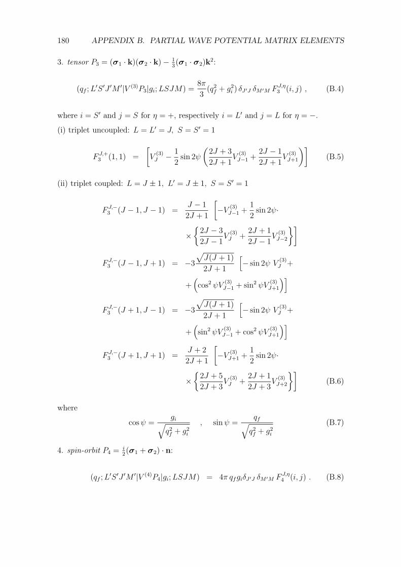
180 APPENDIX B. PARTIAL WAVE POTENTIAL MATRIX ELEMENTS

3. tensor P3 = (σ1 · k)(σ2 · k)− 13(σ1 · σ2)k

2:

(qf ;L′S ′J ′M ′|V (3)P3|gi;LSJM) =

8π

3(q2f + g2i ) δJ ′J δM ′M F J,η

3 (i, j) , (B.4)

where i = S ′ and j = S for η = +, respectively i = L′ and j = L for η = −.

(i) triplet uncoupled: L = L′ = J, S = S ′ = 1

F J,+3 (1, 1) =

[V

(3)J − 1

2sin 2ψ

(2J + 3

2J + 1V

(3)J−1 +

2J − 1

2J + 1V

(3)J+1

)](B.5)

(ii) triplet coupled: L = J ± 1, L′ = J ± 1, S = S ′ = 1

F J,−3 (J − 1, J − 1) =

J − 1

2J + 1

[−V (3)

J−1 +1

2sin 2ψ·

×2J − 3

2J − 1V

(3)J +

2J + 1

2J − 1V

(3)J−2

]

F J,−3 (J − 1, J + 1) = −3

√J(J + 1)

2J + 1

[− sin 2ψ V

(3)J +

+(cos2 ψV

(3)J−1 + sin2 ψV

(3)J+1

)]F J,−3 (J + 1, J − 1) = −3

√J(J + 1)

2J + 1

[− sin 2ψ V

(3)J +

+(sin2 ψV

(3)J−1 + cos2 ψV

(3)J+1

)]F J,−3 (J + 1, J + 1) =

J + 2

2J + 1

[−V (3)

J+1 +1

2sin 2ψ·

×2J + 5

2J + 3V

(3)J +

2J + 1

2J + 3V

(3)J+2

](B.6)

where

cosψ =gi√q2f + g2i

, sinψ =qf√q2f + g2i

(B.7)

4. spin-orbit P4 =i2(σ1 + σ2) · n:

(qf ;L′S ′J ′M ′|V (4)P4|gi;LSJM) = 4π qfgiδJ ′J δM ′M F J,η

4 (i, j) . (B.8)

181

(i) triplet uncoupled: L = L′ = J, S = S ′ = 1

F J,+4 (1, 1) = −

(V

(4)J−1 − V

(4)J+1

)/(2J + 1) (B.9)

(ii) triplet coupled: L = J ± 1, L′ = J ± 1, S = S ′ = 1

F J,−4 (J − 1, J − 1) =

(J − 1)

(2J − 1)

(V

(4)J−2 − V

(4)J

)F J,−4 (J + 1, J + 1) = − (J + 2)

(2J + 3)

(V

(4)J − V

(4)J+2

)(B.10)

5. antisymmetric spin-orbit P6 =i2(σ1 − σ2) · n:

(qf ;L′S ′J ′M ′|V (6)P6|gi;LSJM) = 4π qfgiδJ ′J δM ′M F J,η

6 (S ′, S) . (B.11)

(i) singlet-triplet uncoupled: L = L′ = J, S = 0, S ′ = 1

F J,+6 (1, 0) = F J,+

6 (0, 1) =

√J(J + 1)

2J + 1

(V

(6)J−1 − V

(6)J+1

). (B.12)

Using these matrix elements, the partial waves for the potentials can be calculated

for the pseudo-scalar, the vector,and the scalar meson-exchange potentials. Follow-

ing [116], henceforth the following short hand notation we will use for the potentials:

(i) P = (−)J :

V J0,0 = V J,+(0, 0) , V J

0,2 = V J,+(0, 1)

V J2,0 = V J,+(1, 0) , V J

2,2 = V J,+(1, 1) (B.13)

(ii) P = −(−)J :

V J1,1 = V J,−(J − 1, J − 1) , V J

1,3 = V J,−(J − 1, J + 1)

V J3,1 = V J,−(J + 1, J − 1) , V J

3,3 = V J,−(J + 1, J + 1) (B.14)

where qf and qi are the final and initial momenta. So V J0,0 = V J

0,0(qf , qi) etc. Since

182 APPENDIX B. PARTIAL WAVE POTENTIAL MATRIX ELEMENTS

rotational invariance implies

V J2,0(qf , qi) = V J

0,2(qi, qf ) , V J3,1(qf , qi) = V J

1,3(qi, qf ) (B.15)

the off-diagonal terms will be mentioned only for the explicit expressions like V J0,2(qf , qi)

and V J1,3(qf , qi).

Appendix CLSJM Representation Operators

In this Appendix, a description about LSJM operators is given following [106] in

SYM convention [128]. In the SYM-convention the spherical wave functions in

momentum space with quantum numbers J , L, S, is given by

YMJLS(p) = iL CJ L S

M m µYLm (p)χS

µ (C.1)

where χ is the two-nucleon spin wave function. Here the configuration space basic

JLS-states are YMJLS(r) = CJ

MLm

SµY

Lm (r)χS

µ . Transformation to momentum space

results in (C.1). Then

(S · p)YMJLS(p) = −

√6 i (−)L

√

L

2L− 1

L S J

1 1 0

L− 1 S J

YMJL−1S(p)

+

√L+ 1

2L+ 3

L S J

1 1 0

L+ 1 S J

YMJL+1S(p)

where the 9j-symbols differ from [127], formula (6.4.4), in the replacement of the 3j-

symbols by the Clebsch-Gordan coefficients and by leaving out the m33-summation

183

184 APPENDIX C. LSJM REPRESENTATION OPERATORS

(see [133]). The calculation will lead to

(S · p)YMJJ−11(p) = −i aJ YM

JJ1(p)

(S · p)YMJJ+11(p) = i bJ YM

JJ1(p) (C.2)

(S · p)YMJ J 1(p) = i aJ YM

JJ−11(p)− i bJ YMJJ+11(p) ,

where

aJ = −√

J + 1

2J + 1, bJ = −

√J

2J + 1. (C.3)

Using usual ordering of states L = J − 1, L = J, L = J + 1 , the matrix form can

be formed asL = J − 1

J

J + 1

∥∥∥∥∥∥∥∥∥S · p

∥∥∥∥∥∥∥∥∥L = J − 1

J

J + 1

=

0 iaJ 0

−iaJ 0 ibJ

0 −ibJ 0

. (C.4)

Similarly, using for −i(qf × qi) · S for spherical components the formula

− i(qf × qi)n = −4π

3

√2 C111

klnY1k (qf )Y

1l (qi) , (C.5)

the partial wave matrix elements of the operator can be worked out.

These all together give the partial wave projections for the spin triplet states:

(L′1J |V (k2) (S · qi)2 |L1J) = 4π

a2JVJ−1 0 −aJbJVJ−1

0 VJ 0

−aJbJVJ+1 0 b2JVJ+1

(L′1J |(S · qf )2V (k2)|L1J) = 4π

a2JVJ−1 0 −aJbJVJ+1

0 VJ 0

−aJbJVJ−1 0 b2JVJ+1

185

(L′1J |(S · qf )V (k2)(S · qi)|L1J) = 4π

a2JVJ 0 −aJbJVJ

0 a2JVJ−1 + b2JVJ+1 0

−aJbJVJ 0 b2JVJ

and

(L′1J |−i(qf×qi)·SV (k2)|L1J) = 4π

2J + 1

(J − 1) (VJ−2 − VJ) , L = L′ = J − 1

− (VJ−1 − VJ+1) , L = L′ = J

−(J + 2) (VJ − VJ+2) , L = L′ = J + 1

Considering the identity

(σ1 · a)(σ2 · a) = 2(S · a)2 − a2 , (C.6)

the tensor operator can be written as

P3 = (σ1 · k)(σ2 · k)−1

3(σ1 · σ2) =

1

3

[g2i S12(qi) + q2f S12(qf )

]−4 (S · qf ) (S · qi) + 2i (qf × qi) · S+

4

3(qf · qi)S

2 (C.7)

where the momentum-space tensor-operator S12 is defined in Eq. 3.52. From the

formulas given in this appendix the partial wave projections of the several potential

forms of scalar, pseudo-scalar , and vector mesons can be derived in a straightforward

manner.

Appendix DPartial Wave Decomposition of NN

We introduce the following notation for the R- matrix elements in LSJM basis

L,L′RJ = ⟨L′SJM |RJ |LSJM⟩ (D.1)

and the + for L,L’= J+1 and − for L,L’= J-1. The partial wave elements can be

obtained from the helicity basis elements by the following unitary transformations

[59]

0RJ =0 RJ (D.2)

1RJ =1 RJ (D.3)

++RJ = 12J+1

[(J + 1)12RJ + J 34RJ − 2√

J(J + 1)(5RJ +6 RJ)] (D.4)

−−RJ = 12J+1

[J12RJ + J (J + 1)34RJ + 2√

J(J + 1)(5RJ +6 RJ)] (D.5)

+−RJ = − 12J+1

[√

J(J + 1)(12RJ −34 RJ) + 2(J + 1)5RJ − 2J 6RJ ] (D.6)

−+RJ = − 12J+1

[√

J(J + 1)(12RJ −34 RJ)− 2J5RJ − 2(J + 1) 6RJ ] (D.7)

According to the transformation, the uncoupled spin singlet 0RJ and the corres-

ponding uncoupled spin triplet element 1RJ are same in both the representations

and in more explicit formulation is given by

0RJ(q′,q | E) =0 V J(q′,q | E)+P∑i

∫dk

2π20V J(q′,ki | E)G(ki,qi)

0RJ(ki,q | E)

(D.8)

187

Appendix EHelicity State Basis Decomposition

The baryons being a spin-12particles, the spin also need to be taken into account.

In order to treat the spin accordingly, the helicity basis representation is a conveni-

ent method. Here we briefly describe the helicity basis representation used in our

numerical calculation, for representation purposes. A more detailed description on

the subject can be found in [59]. The helicity H of a particle is defined as in [59]

H =S · p

|S| · |p|(E.1)

where S is the spin and p is the momentum of the particle. Physically it implies

the projection of spin of the particle to the direction of the momentum, when the

spin is parallel to momentum, the helicity is denoted by positive (+) sign and called

”right-handed” , where as for anti-parallel motion, it is negative (−) and termed as

”left-handed”. For a spin-12particle, the eigenvalue λi of the helicity operator (Eq.

E.1) of particle i can have two possible values: ±12. In the following, we denote,

12as + and −1

2as - . The R-matrix equation in helicity basis, after partial wave

decomposition for a state with total angular momentum J, is given by,

⟨λ′1λ′2|RJ |λ1λ2⟩

= ⟨λ′1λ′2|V J |λ1λ2⟩

+∑h1h2

P

∫k2dk

2π2⟨λ′1λ′2|V J |h1h2⟩ G12 ⟨h′1h′2|RJ |λ1λ2⟩ (E.2)

189

190 APPENDIX E. HELICITY STATE BASIS DECOMPOSITION

The momentum dependence of R is suppressed here. Here the summation is over

different helicity states hi of particle 1 and 2. λ′1, λ′2 are the final and λ1, λ2 are the

initial helicities of the particles involved in scattering. From now on we represent

only the absolute value of the three-momenta denoted as q = |q|, q′ = |q’|,and

k = |k|. Here the execution of the angle integration leaves Eq. 4.4 in one-dimensional

form with a leading factor of 4πk2. We now re-write re-introduce the function

Green’s function G12 as G as following,

G (k,q) =2µ12k

2

q2 − k2 + iϵ(E.3)

and rewrite the above R-matrix equation in helicity basis as

⟨λ′1λ′2|RJ |λ1λ2⟩ = ⟨λ′1λ′2|V J |λ1λ2⟩

+∑h1h2

P∫

dk

2π2⟨λ′1λ′2|V J |h1h2⟩ G ⟨h′1h′2|RJ |λ1λ2⟩ (E.4)

where the k2 is now not shown explicitly but taken care of of by G. This equation is

a coupled integral equation. Ignoring antiparticles following [59] , there are 4X4=16

helicity amplitudes of RJ . Taking into account the conservation principle followed

by the strong interaction, namely, parity, total spin, and time reversal, the number

of independent amplitudes reduced to only six. Following Machleidt’s convention

[59], these can be represented as

0RJ = ⟨++ |RJ ++⟩ − ⟨++ |RJ −−⟩ (E.5)

1RJ = ⟨+− |RJ +−⟩ − ⟨+− |RJ −+⟩ (E.6)

12RJ = ⟨++ |RJ ++⟩+ ⟨++ |RJ −−⟩ (E.7)

34RJ = ⟨+− |RJ +−⟩+ ⟨+− |RJ −+⟩ (E.8)

5RJ = ⟨++ |RJ +−⟩ (E.9)

6RJ = ⟨+− |RJ ++⟩ (E.10)

with ± representing ±12helicity states. For a more detailed derivation, one can look

at [59]. Similar representation exists for the potential matrix elements ⟨λ′1λ′2|V (q′,q |

191

E)|λ1λ2⟩. The R-matrix equation now can be solved in this form, however, The

hyperon-model derived here is fitted to the partial wave analyzes of the hyperon-

baryon scattering data. Hence the integral equation for the scattering amplitude

defined above, must be solved in partial wave basis. Here we define the transforma-

tion of the integral equation on the plane wave basis of the integral equation to the

partial wave basis, commonly referred to as the LSJM basis. In next section, we

discuss the relation between these representations.

Bibliography

[1] M. Agniso et al. [FINUDA Collaboration], Nucl. Phys. A 881 (2012) 269.

[2] C. Rappold et al. [HypHI Collaboration], Phys. Lett. B 728 (2014) 543.

[3] C. Rappold et al. [HypHI Collaboration], On the measured lifetime of light hy-

pernuclei 3ΛH and 4ΛH , Phys. Lett. B 747 (2015) 129.

[4] N. Shah, Y. G. Ma, J. H. Chen and S. Zhang, Production of multistrange had-

rons, light nuclei and hypertriton in central Au+Au collisions at√sNN = 11.5

and 200 GeV, Phys. Lett. B 754 (2016) 6.

[5] Z. L. She, G. Chen, H. g. Xu, T. t. Zeng and D. k. Li, Properties of light

(anti)nuclei and (anti) hypertriton production in Pb-Pb collisions at√sNN =

2.76 TeV, [arXiv:1509.06493].

[6] Integrated Publishing, Inc.

[7] Paulo F. Bedaque, Andrew W. Steiner, Hypernuclei and the hyperon problem

in neutron stars, Phys. Rev. C 92, 025803 (2015) [arXiv:1412.8686v1];

Y Lim, CH Hyun, K Kwak, CH Lee, Hyperon puzzle of neutron stars with Skyrme

force models, Int. J. Mod. Phys. E 24, 1550100 (2015).

[8] M. Danysz, J. Pniewski, Phil. Mag. 44 (1953) 348.

[9] R. Machleidt, K. Holinde and Ch. Elster, The bonn meson-exchange model for

the nucleon-nucleon interaction, Phys. Rep. 149, 1 (1987).

193

194 BIBLIOGRAPHY

[10] W. N. Cottingham, M. Lacombe, B. Loiseau, J. M. Richard and R. Vinhman,

Nucleon-Nucleon interaction from pion-nucleon phase-shift analysis, Phys. Rev.

D 8, 800 (1973).

[11] V. G. J. Stoks, R. A. M. Klomp, C. P. F. Terheggen, and J. J. de Swart,

Construction of high-quality NN potential models, Phys. Rev. C 49 (1994), 2950-

2962.

[12] Murray Gell-Mann The Eightfold Way: A Theory of strong interaction sym-

metry, CTSL-20, TID-12608.

[13] Yuval Ne’eman, Derivation of strong interactions from a gauge invariance, Nucl.

Phys. 26 (1961) 222-229.

[14] Murray Gell-Mann, A Schematic Model of Baryons and Mesons , Phys. Lett. 8

(1964) 214-215.

[15] G Zweig, An SU(3) model for strong interaction symmetry and its breaking,

Feb 21, 1964, CERN-TH-401.

[16] K.A. Olive et al. (Particle Data Group), Chin. Phys. C, 38, 090001 (2014) and

2015.

[17] NN-online.org, May, 2016.

[18] Samuel S. M. Wong, Introductory Nuclear Physics, Second Edition, Wiley-VCH

Verlag GmbH and Co. KGA, Weinheim, 2004.

[19] T. Furumoto, Y. Sakuragi, Y. Yamamoto, Hyperon-nucleus folding potentials

in the complex G-matrix approach, Nucl. Phys. A 835, 362 (2010);

Yasuo Yamamoto, Toshio Motoba and Thomas A. Rijken, G-Matrix Approach to

Hyperon-Nucleus Systems, Prog. Theor. Phys. Supplement 185 (2010) 72-105.

[20] M Naghdi, Nucleon-nucleon interaction: A typical/concise review,

[arXiv:0702078];

R. Machleidt, I. Slaus, The Nucleon-nucleon interaction, J. Phys. G 27: R69-R108

(2001) [ arXiv:0101056v1].

BIBLIOGRAPHY 195

[21] Anwar Kamal, Nuclear Physics, Springer, United States, 2014.

[22] Peter Ring, Peter Schuck , The Nuclear Many-Body Problem, Springer, 1980.

[23] E. Hiyama, S. Ohnishi, M. Kamimura, Y. Yamamoto, Four-body structure of

neutron-rich hypernucleus 6ΛH , [arXiv:1304.0317v1].

[24] E. Hiyama, M. Kamimura, T. Motoba, T. Yamada, Y. Yamamoto, Λ − Σ

conversion in based on four-body calculation, Phys. Rev. C 65 (2002) 011301.

[25] Masahiro Isaka, Masaaki Kimura, Akinobu Dote, Akira Ohnishi, De-

formation of hypernuclei studied with antisymmetirzed molecular dynamics,

Phys.Rev.C83:044323,2011

[26] K. Miyagawa et al., Phys. Rev. C 74, 034002 (2006).

[27] D. Gazda, J. Mares , P. Navratil, R. Roth ,R. Wirth, No-Core Shell

Model for Nuclear Systems with Strangeness, Phys. Rev. C 88, 035208 (2013)

.[arXiv:1312.0478v1].

[28] J. S. Liang and H. Shen, Medium modifications of baryon properties in nuclear

matter and hypernuclei, [arXiv:1304.4713v3].

[29] Y. Yamamoto, T. Furumoto, N. Yasutake, and Th.A. Rijken, Hyperon-mixed

neutron star with universal many-body repulsion, [arXiv:1510.06099v1].

[30] R.O. Gomes, V.A. Dexheimer, S. Schramm, C.A.Z. Vasconcellos, Many-body

forces in the equation of state of hyperonic matter, [arXiv:1411.4875v1].

[31] I. Vidana, Single-particle spectral function of the Λ hyperon in finite nuclei,

[arXiv:1603.05635v1]

[32] Francesca Sammarruca, Effects of Λ hyperons on the nuclear equation of state

in a Dirac-Brueckner-Hartree-Fock model, Phys. Rev. C 79 : 034301, 2009

[33] H. Chen, M. Baldo, G. F. Burgio, and H.-J. Schulze, Hybrid stars with the

Dyson-Schwinger quark model, [arXiv:1107.2497v2].

196 BIBLIOGRAPHY

[34] E. N. E. van Dalen, G. Colucci, and A. Sedrakian, Phys. Lett. B 734, 383

(2014).

[35] H. Lenske, C. Fuchs, Phys.Lett. B 345 355 (1995)

[36] S. Petschauer, J. Haidenbauer, N. Kaiser, Ulf-G. Meißner, W. Weise, Hyperons

in nuclear matter from SU(3) chiral effective field theory, Eur. Phys. J. A (2016)

52: 15

[37] H. Togashi, E. Hiyama, Y. Yamamoto, and M. Takano, Equation of state for

neutron stars with hyperons by the variational method, [arXiv:1602.08106].

[38] E E Kolomeitsev, K AMaslov, D N Voskresensky, Hyperon puzzle and the RMF

model with scaled hadron masses and coupling constants, [arXiv:1509.06312v1].

[39] K. A. Maslov, E. E. Kolomeitsev and D. N. Voskresensky, Relativistic Mean-

Field Models with Scaled Hadron Masses and Couplings: Hyperons and Maximum

Neutron Star Mass, [arXiv:1509.02538v2].

[40] Ulf-G. Meißner, Johann Haidenbauer, Foundations of Strangeness Nuclear

Physics derived from chiral Effective Field Theory, [arXiv:1603.06429v1].

[41] Diego Lonardoni, Alessandro Lovato, Stefano Gandolfi, and Francesco Pederiva,

Hyperon Puzzle: Hints from QuantumMonte Carlo Calculations, Phys. Rev. Lett.

114, 092301 (2015) [arXiv:1407.4448v2].

[42] Tsuyoshi Miyatsu and Myung-Ki Cheoun, Equation of state for neutron

stars with hyperons and quarks in relativistic Hartree-Fock approximation,

[arXiv:1506.05552].

[43] I. Tews, S. Gandolfi, A. Gezerlis, A. Schwenk, Quantum Monte Carlo calcula-

tions of neutron matter with chiral three-body forces, Phys. Rev. C 93, 024305

(2016).

[44] Sinya Aoki, Takumi Doi, Tetsuo Hatsuda, Yoichi Ikeda, Takashi Inoue, Noriy-

oshi Ishii, Keiko Murano, Hidekatsu Nemura, Kenji Sasaki, Lattice QCD approach

to Nuclear Physics, [arXiv:1206.5088].

BIBLIOGRAPHY 197

[45] S. R. Beane, E. Chang, S. D. Cohen, W. Detmold, H.-W. Lin, T. C. Luu, K. Or-

ginos, A. Parreno, M. J. Savage, A. Walker-Loud, Hyperon-Nucleon Interactions

and the Composition of Dense Nuclear Matter from Quantum Chromodynamics,

[arXiv:1204.3606].

[46] B. Holzenkamp, K. Holinde, and J. Speth, Nucl. Phys. A500, 485 (1989)

[47] A. Reuber, K. Holinde and J. Speth, Nucl. Phys. A 570 (1994) 543

[48] J. Haidenbauer, U.-G. Meißner, Phys. Rev. C 72 (2005) 044005

[49] V. G. J. Stoks and Th. A. Rijken, Soft-core baryon-baryon potentials for the

complete baryon octet, Phys. Rev. C 59 (1999), no. 6, 3009-3020

[50] Th. A. Rijken, V. G. J. Stoks, and Y. Yamamoto, Soft-core hyperon-nucleon

potentials, Phys. Rev. C 59 (1999), no. 1, 21-40

[51] Th.A. Rijken and Y. Yamamoto, Extended-soft-core Baryon-Baryon Model. II.

Hyperon-Nucleon Interaction, Phys. Rev. C 73 , 044008 (2006).

[52] Hideki Yukawa, On the Interaction of Elementary Particles , Proc. Phys. Math.

Soc. Jap. 17 (1935) 48.

[53] R. B. Wiringa, V. G. J. Stoks, and R. Schiavilla Phys. Rev. C 51, 38-51 (1995)

[54] V.G.J. Stoks, R.A.M. Klomp, C.P.F. Terheggen, J.J. de Swart, Construction

of high-quality Nucleon-Nucleon potential models Phys.Rev.C49:2950-2962,1994

[55] R. Machleidt , The high-precision, charge-dependent Bonn nucleon-nucleon po-

tential (CD-Bonn),Phys.Rev. C63 (2001) 024001

[56] J.J. de Swart, Rev. Mod. Phys. 35, 916 (1963); ibid. 37, 326(E) (1965)

[57] H. Bethe, E. Salpeter (1951), ”A Relativistic Equation for Bound-State Prob-

lems”, Physical Review 84 (6), 1232

[58] R. Blankenbecler and R. Sugar, Linear Integral Equations for Relativistic Mul-

tichannel Scattering, Phys. Rev. 142 (1966), 1051-1059

198 BIBLIOGRAPHY

[59] R. Machleidt, ”One-Boson Exchange Potentials and Nucleon-Nucleon Scatter-

ing”, Computational Nuclear Physics 2: Nuclear Reactions, Springer- Verlag, New

York, 1993

[60] Christoph Marcus Keil, Microscopic baryon-baryon interactions at finite dens-

ity and hypernuclear structure, Ph.D. thesis, Justus-Liebig-Universitat Gießen,

unpublished (2004)

[61] K. Erkelenz, R. Alzetta, and K. Holinde, Momentum space calculations and

helicity formalism in nuclear physics, Nuclear Physics A 176 (1971), no. 2, 413 -

432.

[62] R. Machleidt, K. Holinde, and Ch. Elster, Phys. Rep. 149, 1 (1987).

R. Machleidt, Adv. Nucl. Phys. 19, 189 (1989).

[63] E. Epelbaum, H.-W. Hammer, and Ulf-G. Meißner, Modern theory of nuclear

forces, Rev. Mod. Phys. 81 (2009), 1773-1825

[64] R. B. Wiringa, V. G. J. Stoks, and R. Schiavilla Phys. Rev. C 51, 38-51 (1995)

[65] R. Machleidt, Computational Nuclear Physics 2-Nuclear Reactions, ch. 1, pp.

1-29, Springer, New York, 1993.

[66] F. Eisele, H. Filthuth, W. Foehlisch, V. Hepp, G. Zech, Phys. Lett. 37B (1971),

204.

[67] H.G. Dosch, R. Engelmann, H. Filthuth, V. Hepp, E. Kluge, Phys. Lett. 21

(1966), 236.

[68] G. Alexander, U. Karshon, A. Shapira, G. Yekutieli, R. Engelmann, H.

Filthuth, W. Lughofer, Phys. Rev. 173 (1968), 1452.

[69] L. Piekenbrock, F. Oppenheimer, Phys. Rev. Lett. 12 (1964), 625.

[70] Thomas H. Groves, Phys. Rev. 129 (1963), 1372

[71] J.A. Kadyk, G. Alexander, J.H. Chan, P. Gaposchkin, G.H. Trilling,Nucl. Phys.

B27 (1971), 13.

BIBLIOGRAPHY 199

[72] J.M. Hauptmann, J.A. Kadyk, G.H. Trilling, Nucl. Phys. B125 (1977), 29.

[73] H.A. Rubin, R.A. Burnstein,Phys. Rev. 159 (1967), 1149.

[74] B. Sechi-Zorn, B. Kehoe, J. Twitty, R.A. Burnstein, Phys. Rev. 175 (1968),

1735.

[75] R. Engelmann, H. Filthuth, v. Hepp, G. Zech, Phys. Lett. 37B (1971) 204.

[76] V. Hepp and H. Schleich, Z. Phys. 214 (1968) 71.

[77] D. Stephen, Ph.D. thesis, University of Massachusetts, unpublished (1970).

[78] P. M. M. Maessen, Th. A. Rijken, and J. J. de Swart, Phys. Rev. C 40, 2226

(1989).

[79] M.M. Nagels, T.A. Rijken, and J.J. de Swart, Ann. Phys. (N.Y.) 79, 338 (1973)

[80] D. Cline, R. March, M. Sheaff, Phys. Lett. 25B (1967), 446.

[81] R.G.E. Timmermans, Th.A. Rijken, and J.J. de Swart, Phys. Lett. B 257, 227

(1991)

[82] Anika Obermann, Master Thesis, Universoty of Giessen, unpublished (2011).

[83] M.A. Preston and R.K. Bhaduri, Structure of the Nucleus, Westview Press,

1993.

[84] P.J. Ellis, R. Knorren and M. Prakash, Phys. Lett. B349, 11 (1995).

[85] J. Schaffner and I. Mishustin, Phys. Rev. C 53, 1416 (1996)

[86] S. Balberg and A. Gal, Nucl. Phys. A625, 435 (1997).

[87] H.-J. Schulze, A. Lejeune, J. Cugnon, M. Baldo, and U. Lombardo, Phys. Lett.

B355, 21 (1995).

[88] H.-J. Schulze, M. Baldo, U. Lombardo, J. Cugnon, A. Lejeune, Phys. Rev. C57,

704 (1998).

200 BIBLIOGRAPHY

[89] P.B. Demorest, T.T. Pennucci, S.M. Ransom, M.S.E. Roberts, J.W.T. Hessels,

Nature 467, 1081 (2010).

[90] J. Antoniadis et al., Science 340, 1233232 (2013).

[91] Alessandro Drago et al., Phys. Rev. C90 (2014) no. 6,065809.

[92] David Blaschke et al., AIP COnf. Proc. 1701 (2016) 020013.

[93] H. Lenske, Density Dependent Relativistic Field Theory, Lect. Notes. Phys.

641, 147-174 (2004).

[94] S. Weissenborn, D. Chatterjee, and J. Schaffner-Bielich, Hyperons and massive

neutron stars: Vector repulsion and SU(3) symmetry, Phys. Rev. C 85, 065802

(2012);

S. Weissenborn, D. Chatterjee, and J. Schaffner-Bielich, Hyperons and massive

neutron stars: the role of hyperon potentials, Nucl. Phys. A 881, 62 (2012).

[95] Y. Yamamoto, T. Furumoto, N. Yasutake, and T. A. Rijken, Hyperon mixing

and universal many-body repulsion in neutron stars, Phys. Rev. C 90, 045805

(2014).

[96] D. Lonardoni, A. Lovato, S. Gandolfi, and F. Pederiva, Phys. Rev. Lett. 114,

092301 (2015).

[97] M. I. Haftel and F. Tabakin, Nucl. Phys. A 158 (1970).

[98] V. G. J. Stoks and Th. A. Rijken, Phys. Rev. C 59 (1999) 3009-3020

[arXiv:9901028]

[99] H.P. Stapp, Phys. Rev. 103 (1956) 425

[100] J. Haidenbauer, U.-G. Meißner, A. Nogga, H. Polinder, Lect. Notes Phys. 724

(2007) 113;

J. Haidenbauer, U.-G. Meißner, Phys.Lett. B684 (2010) 275-280.

[101] J. Haidenbauer, S. Petschauer, N. Kaiser, U.-G. Meißner, A. Nogga, W. Weise,

Nucl.Phys. A915, 24 (2013), [arXiv:1304.5339v1]

BIBLIOGRAPHY 201

[102] J. Haidenbauer, Ulf-G. Meißner, S. Petschauer, Strangeness S = -2 baryon-

baryon interaction at next-to-leading order in chiral effective field theory,

[arXiv:1511.05859].

[103] MINUIT, CERN Program Library entry D506, CERN, Geneva.

[104] E. Anderson, Z. Bai, C. Bischof, L. S. Blackford, J. Demmel, J. Dongarra,

J. Du Croz , A. Greenbaum, S. Hammarling, A. McKenney and D. Sorensen,

LAPACK Users’ Guide, Third Edition, Society for Industrial and Applied Math-

ematics, Philadelphia, PA, 1999.

[105] Y. Fujiwara, C. Nakamoto, Y. Suzuki, Phys. Rev. 54 (1996) 2180;

M. Kohno, et al., Nucl. Phys. A 674 (2000) 229;

Y. Fujiwara , Y. Suzuki , C. Nakamoto, Prog. Part. Nucl. Phys. 58 (2007) 439;

M. Oka, K. Shimizu and K. Yazaki, Prog. Theor. Phys. S137 (2000).

[106] H. Polinder, J. Haidenbauer and U.-G. Meißner, Nucl. Phys. A 779, 244 (2006);

H. Polinder, J. Haidenbauer and U.-G. Meißner, Phys. Lett. B 653, 29 (2007).

[107] C. M. Vincent, S. C. Phatak, Phys. Rev. C 10 (1974) 391.

[108] P.J. Ellis, R. Knorren and M. Prakash, Phys. Lett. B349, 11 (1995).

[109] J. Schaffner and I. Mishustin, Phys. Rev. C 53, 1416 (1996).

[110] E. Epelbaum, H. W. Hammer, and U.-G. Meisner, Rev. Mod. Phys. 81 (2009)

1773;

R. Machleidt and D. R. Entem, Phys. Rept. 503 (2011) [arXiv:1105.2919].

[111] Siegmund Brandt, Data Analysis: statistical and computational methods for

scientists and engineers, Third Edition, Springer Publisher GMBH, New York,

1998. Statistical and Computational Methods for Scientists and Engineers

[112] F. James, MINUIT Function Minimization and Error Analysis: Reference

Manual Version 94.1, CERN-D-506

202 BIBLIOGRAPHY

[113] Hendrik Polinder, Strong Meson-Baryon Interactions, A soft-core model for

low- and intermediate-energy π-nucleon and K+-nucleon scattering, Ph.D. thesis,

University of Nijmegen, 2004, ISBN 90-9017742-6.

[114] W. S. C. Williams, An Introduction to Elementary Particles, Second Edition,

Academic Press, New York and London, 1971.

[115] P. M. M. Maessen, T. A. Rijken, J. J. de Swart, Phys. Rev. C 40 (1989) 2226.

[116] T. A. Rijken, Ann. Phys. (NY) 164, 1 and 23 (1985).

[117] J. J. de Swart, M. M. Nagels, T. A. Rijken, and P. A. Verhoeven, Springer

tracts in Modern Physics, Vol. 60, 137 (1971).

[118] P.M.M. Maessen, T.A. Rijken, and J.J. de Swart, Phys. Rev. D 40, 2226

(1989).

[119] P. S. Signell and R. E. Marshak, Phys. Rev. 106, 832 (1957); 109, 1229 (1958).

[120] S. Okubo and R. E. Marshak, Ann. Phys. (NY) 4, 166 (1958).

[121] Tao Pang, An Introduction to Computational Physics, Cambridge University

Press, Cambridge, UK, 2006.

[122] G. D. Rochester and C. C. Butler, Nature 160 (1947) 855.

[123] J. H. Christenson, J. W. Cronin, V. L. Fitch, and R. Turlay, Evidence for the

2π Decay of the K02 Meson, Phys. Rev. Lett. 13, 138 (1964).

[124] O. Hashimoto, H. Tamura, Prog. Part. Nucl. Phys. 57 (2006) 564.

[125] Charles J. Joachain, Quantum Collision Theory, North-Holland Pub. Co.,

1975.

[126] K.A. Olive et al. (Particle Data Group), Chin. Phys. C, 38, 090001 (2014) and

2015 update.

[127] A.R. Edmonds, Angular Momentum in Quantum Mechanics, (Princeton Uni-

versity Press, Princeton (1957)).

BIBLIOGRAPHY 203

[128] H. P. Stapp, T. J. Ypsilantis, M. Metropolis, Phys. Rev. 105 (1957) 302.

[129] H. Lenske, M. Dhar, T. Gaitanos, SU(3) Approach to Hypernuclear Interac-

tions and Spectroscopy, [arXiv:1602.08917].

[130] H. Lenske, X. Cao, M. Dhar, T. Gaitanos, R. Shyam, Production and Interac-

tions of Hyperons and Hypernuclei, HYP 2015 Conference Proceedings, Sendai,

Japan, Sept. 7-11, 2015, [arXiv:1603.00298].

[131] M. Dhar, H. Lenske, in preparation.

[132] H. Lenske, M. Dhar, N. Tsoneva, J. Willhelm, Exotic nuclear matter, EPJ

Web Conf. 107 (1026) 10001.

[133] The explicit relation between 9j-symbols used here and those in [127]

Eq. (6.4.4) is the following

j11 j12 j13

j21 j22 j23

j31 j32 j33

= (−)j31+j13−j32−j23 [(2j13 + 1)(2j31 + 1)(2j23 + 1)(2j32 + 1)]1/2

×

j11 j12 j13

j21 j22 j23

j31 j32 j33

Acknowledgment

First I want to express my deep gratitude towards to my supervisor Prof. Dr. Horst

Lenske without whom this thesis would never have been possible. For the interesting

research topic that he has suggested for the dissertation, for the fruitful discussions,

help, and guidance throughout these years not only regarding physics but also for

other related or irrelevant matters, I would like to sincerely thank him. I want to

thank also for believing an international student and showing the trust that let me

come and work with him in Germany. The days I spent here enriched me in many

ways of my life helping me to grow. I am very much grateful to my supervisor for

introducing me to the world physics community by recommending the conferences

I should be attending. Last, a special mention should be on his immense help and

support during the time when I had a leg fracture that provided me the strength to

recover soon.

I would like to acknowledge HGS-HIRe for FAIR facility for providing the finan-

cial support for this work.

Next person contributing the most in this thesis is Prof. Johann Haidenbauer.

I would like to thank him for providing important opinion on construction of the

model, sharing his insights about the difficulties involved but always with a possible

solution to that, replying to my e-mails with utmost care, all in all guiding me in

achieving the proper results.

Prof. Dr. Christian Fischer is also someone whom I would like to express my

deep gratitude too for providing the necessary support always, especially at the last

stage of the work, regarding visa, defense, and more.

206 BIBLIOGRAPHY

I would like to thank Prof. Terry Mart for providing the MINUIT source code

and generously explaining how to use the facility.

Steffi, Rainer, Alessia, Christian, Jan Haas, Richard, Walter, Jan Lucker: I thank

each of them for making my stay wonderful and enjoyable in Germany far from my

family and friends. A big thanks to Rainer for always being there in crisis and

Alessia for the lovely dinners we had, the lovely times we had spent, and for being

the lovely friend she has been always. The lunches at the ’Tee-Kuche’ were the best

parts of the stay.

I thank Christian, Alessia, and Richard wholeheartedly for helping me in sub-

mitting the thesis to prufungsamt while I am away, and Rainer for providing the

German translated abstract.

I would also like to thank Prof. S P Khastgir for actually introducing me to

the world of ’real’ physics, for those enlightening words that helped me to keep the

enthusiasm for hard work, the true ’guidance’ he always provided, for teaching in a

way that can not get better, for always there being for any help and suggestion, and

for the proof reading even in quick deadline. Prof. Sayan Kar, Prof. A K Singh,

Prof. K L Panigrahi, and Prof. Anushree Roy are also acknowledged for always

providing the inspiration for doing good work.

For indirect support, I would like to mention Somnathda for passing useful tips

on writing thesis, Subhashishda for providing the thesis template, Stans also for

the same, and Narayan for giving useful tips on hard times and for the quick proof

reading.

I would like to thank the secretaries of Institute of Theoretical Physics, Uni

Gießen, for taking care of the formal affairs efficiently.

A special bunch of thanks towards Ripanda, Binoy Sir, Debajyotida, Laxmanda,

and Atishadi for providing relevant information in getting leave to finish the project.

Anumama is someone whom I would like to express my special gratitude for

giving me the practical tips for finishing the project and all the relevant motivations

he provided.

Last but not the least, I would like to thank my family for everything. I want to

thank my mother for all the sacrifices she did for me, for all the trouble she took to

BIBLIOGRAPHY 207

travel to Delhi along with me each time I fly to Frankfurt, for always motivating to

do progress and finish the thesis, for teaching the principles of life, and for always

being concerned about my health and well-being. My gratitude towards my mother

can not be expressed in words. I also would like to thank my brother, who always

inspired me to do good work, always provided positive vibes, being always there

to take care of the family crisis so that I can concentrate in my work, and during

the last phase kept me going. Thanks. My little nephew, Aarno, is also someone I

would like to thank just for being here to make us happy. A special thanks to my

sister-in-law too for taking care of the family.

Finally, I end by thanking my father, who, wherever today, is the reason for this

thesis and everything I achieved in my life.

Declaration

I declare that I have completed this dissertation single-handedly without the unau-

thorized help of a second party and only with the assistance acknowledged therein.

I have appropriately acknowledged and cited all text passages that are derived ver-

batim from or are based on the content of published work of others, and all inform-

ation relating to verbal communications. I consent to the use of an anti-plagiarism

software to check my thesis. I have abided by the principles of good scientific con-

duct laid down in the charter of the Justus Liebig University Giessen ”Satzung der

Justus-Liebig-Universitat Gießen zur Sicherung guter wissenschaftlicher Praxis” in

carrying out the investigations described in the dissertation.

Gießen, May 2016

Madhumita Dhar

hyperon interaction in free space and nuclear matter...

Documents