hyperdrive: exploring hyperparameters with pop scheduling · 2018-05-24 · hyperdrive: exploring...

HyperDrive: Exploring Hyperparameters with POP SchedulingJeff Rasley

Brown UniversityYuxiong HeMicrosoft

Feng YanUniversity of Nevada, Reno

Olatunji RuwaseMicrosoft

Rodrigo FonsecaBrown University

AbstractThe quality of machine learning (ML) and deep learning (DL) mod-els are very sensitive to many different adjustable parameters thatare set before training even begins, commonly called hyperparame-ters. Efficient hyperparameter exploration is of great importanceto practitioners in order to find high-quality models with afford-able time and cost. This is however a challenging process due toa huge search space, expensive training runtime, sparsity of goodconfigurations, and scarcity of time and resources. We develop ascheduling algorithm POP that quickly identifies among promising,opportunistic and poor configurations of hyperparameters. It infusesprobabilistic model-based classification with dynamic schedulingand early termination to jointly optimize quality and cost. We alsobuild a comprehensive hyperparameter exploration infrastructure,HyperDrive, to support existing and future scheduling algorithmsfor a wide range of usage scenarios across different ML/DL frame-works and learning domains. We evaluate POP and HyperDriveusing complex and deep models. The results show that we speedupthe training process by up to 6.7x compared with basic approacheslike random/grid search and up to 2.1x compared with state-of-the-art approaches while achieving similar model quality comparedwith prior work.

CCS Concepts • Computer systems organization → Cloudcomputing; • Computing methodologies → Machine learn-ing approaches;

Keywords Hyperparameter exploration, cluster scheduling

ACM Reference format:Jeff Rasley, Yuxiong He, Feng Yan, Olatunji Ruwase, and Rodrigo Fonseca.2017. HyperDrive: Exploring Hyperparameters with POP Scheduling. InProceedings of Middleware ’17, Las Vegas, NV, USA, December 11–15, 2017,13 pages.DOI: 10.1145/3135974.3135994

1 IntroductionIn recent years many machine-learning frameworks have beenintroduced to help developers build and train machine learningmodels for solving different artificial intelligence tasks across su-pervised, unsupervised, and reinforcement learning domains [3,6, 9, 10, 15, 31]. The task performance of trained models is very

Permission to make digital or hard copies of all or part of this work for personal orclassroom use is granted without fee provided that copies are not made or distributedfor profit or commercial advantage and that copies bear this notice and the full citationon the first page. Copyrights for components of this work owned by others than theauthor(s) must be honored. Abstracting with credit is permitted. To copy otherwise, orrepublish, to post on servers or to redistribute to lists, requires prior specific permissionand/or a fee. Request permissions from [email protected] ’17, Las Vegas, NV, USA© 2017 Copyright held by the owner/author(s). Publication rights licensed to ACM.978-1-4503-4720-4/17/12. . . $15.00DOI: 10.1145/3135974.3135994

��

� ��

��

�� Figure 1. Performance of 50 randomly selected supervised-learninghyperparameter configurations.

sensitive to many different adjustable parameters, called hyperpa-rameters, which are configured prior to training a model. Examplesof these hyperparameters include learning rate (in many models),number and size of hidden layers in a deep neural network, numberof clusters in k-means clustering, and many more. Hyperparameterexploration searches across different configurations of a model,where each configuration represents a specific set of hyperparam-eter values. Its goal is to find good configurations that optimizethe model performance (e.g., high accuracy, low loss, high reward)with affordable time and cost. This exploration involves two relatedproblems: generating candidate configurations from the large spaceof hyperparameter settings, and actually scheduling and runningthese configurations.

Efficient hyperparameter exploration is of great importance topractitioners in order to improve model performance, reduce train-ing time, and optimize resource usage. This is especially criticalwhen training modern deep and complex learning models withbillions of parameters and millions of training samples on cloudresources. To reach a desired training target, efficient hyperpa-rameter exploration means shorter training time, lower resourceconsumption, and thus lower training costs.

However, it is challenging to design effective scheduling frame-works and algorithms that efficiently explore hyperparameter val-ues while obtaining high model performance and optimizing timeand resource costs. The first key reason is the size of the hyperpa-rameter search space and the expensive training process for eachindividual configuration. Figure 1 shows the model performance(task accuracy) of 50 configurations as a function of iterations overa training dataset for a moderate-size image classification appli-cation CIFAR-10 [20] (detailed experimental setup is presented in§6). Each line in the plot represents a unique configuration. Herewe present only 50 configurations in the plot for clear presenta-tion. Each configuration needs to run about 120 iterations witheach iteration taking about one minute. To fully explore only 50configurations, we need over 4 days of computing. Commonly,models require exploring many more configurations to find high

Middleware ’17, December 11–15, 2017, Las Vegas, NV, USA Rasley et al.

performing hyperparameters. For example, our CIFAR-10 modelhas 14 hyperparameters (such as learning rate, momentum, andweight decay) and most have a continuous range to explore, whichresults in hundreds or thousands (or more) possible configurationsto explore. This problem is even worse when considering largertraining models and datasets, for example, prior work has shownthat a high-quality ImageNet22k image classification model cantake up to ten days to train to convergence using 62 machines [8].Therefore exhaustive search is simply not practical.

A second reason is that, for many models in practice, only fewconfigurations lead to high performance while a majority of config-urations perform very poorly. The results in Figure 1, for example,show that only three configurations are able to exceed 75% accuracy(which is considered reasonable accuracy for this type of simpleCIFAR-10 model that doesn’t do any data augmentation and/or in-tensive preprocessing steps 1), while the majority of configurationsare not able to exceed 20% accuracy. Therefore, simple and popularapproaches such as grid and random hyperparameter generationbet heavily on luck, which results in very inefficient discovery ofhigh performing configurations under reasonable cost and timeconstraints.

Furthermore, optimizing hyperparameter tuning involves manyother factors, such as incorporating different application domaingoals (e.g., supervised, unsupervised, and reinforcement learning)and applicability to different DL/ML frameworks (e.g., Tensorflow,Caffe, and CNTK). It is challenging to design an effective frameworkto support such a wide range of usage scenarios.

Recent work [7, 14, 24] has moved beyond grid-based hyper-parameter generation with adaptive techniques using Bayesianoptimization, which assigns higher probability to areas of the hy-perparameter space that contain likely-good or unknown config-urations. These works do not, however, address how to run theseconfigurations. For example, how long should each configurationrun? Prior work [7, 14, 18, 24, 28] executes each configuration tothe same maximum iteration (which can be a large number of iter-ations), typically ignoring the fact that some configurations couldhave shown their intrinsic value much earlier. As shown in Fig-ure 1, with basic domain knowledge, one can quickly tell that manyconfigurations do not learn at all, with accuracy similar to random( 10% accuracy in this case), which can be identified within fewtraining iterations and terminated early to save resources. In addi-tion, should all running configurations take the same amount ofresources? Clearly, that is not the best way to assign resources sincethe execution progress of the configurations could have offeredmany insights on how well the configurations are likely to perform,thus deserving different amounts of resources. This schedulingproblem of how to effectively map different configurations acrossthe time and space dimension of resources is largely unattended byprior work.

Our work focuses on designing an efficient scheduling algorithmand an effective system framework for hyperparameter exploration.Our scheduling algorithm, POP, dynamically classifies configura-tions into three categories: Promising, Opportunistic, and Poor,and uses these in two major ways. First, along the time dimension,we quickly identify and terminate poor configurations that arenot learning, incorporating application-specific input from modelowners. For example, classification tasks have known non-learning1http://rodrigob.github.io/are_we_there_yet/build/classification_datasets_results.html

random performance values which can be used to prune jobs. Sec-ond, along the space dimension, we use an explore-exploit strategy.We classify promising configurations that are more likely to lead tohigh task accuracy and prioritize them with more resources whilegiving configurations that are still only potentially promising somechances to run – these arewhat we call opportunistic configurations.Unlike prior work [25] that uses instantaneous accuracy only toidentify a fixed set of promising configurations, we incorporate thetrajectory of full learning curves and leverage a probabilistic modelto predict expected accuracy improvement over time as well as pre-diction confidence [11]. The classification and resource allocationbetween promising and opportunistic configurations is dynamic,adjusting the ratio of exploration and exploitation when we observemore predicted and measured results. At the early stage of training,when there is little history information and prediction confidenceis typically low, allocating more resources for exploration helpstraining efficiency. Conversely, at later stages, confidence is higher,and allocating more resources for exploitation can yield higherrewards.

We also design a framework, HyperDrive, which serves as ageneric framework for hyperparameter exploration. HyperDrivelargely decouples the scheduling policy for candidate configura-tions from the type of model and/or framework. It provides an APIthat supports not only our POP scheduling algorithm, but also ex-isting and new ones. It also supports different learning frameworks,such as Caffe [15], CNTK [31], and TensorFlow [3], and learningdomains, such as supervised and reinforcement learning. Lastly,it supports model-owner-defined metrics and inputs to improvescheduling efficiency.

This paper makes the following contributions:

• We develop an efficient scheduling algorithm that infusesprobabilistic model-based configuration classification withdynamic scheduling and early termination (§2 and §3).

• We develop an effective system framework, we call Hy-perDrive, that not only facilitates our proposed schedulingalgorithm, but supports existing and future scheduling al-gorithms, and works with different domains and machinelearning frameworks (§4 and §5).

• We present extensive evaluation of our scheduling algo-rithm and framework using workloads from both super-vised and reinforcement learning domains. We show ourproposed approach outperforms the basic approaches likerandom/grid search by up to 6.7x and outperforms state-of-the-art scheduling techniques by up to 2.1x and that ourframework is practical (§6 and §7).

2 Design Principles of Scheduling AlgorithmHyperparameter exploration is challenging as there are many con-figurations but often much less time and fewer resources. For deepand complex models, it is common that only a small number ofconfiguration choices lead to high quality results. Thus, significantamounts of time and resources could be wasted in searching forgood configurations if considerable attention is not paid to searchefficiency. To enable efficient model exploration and scheduling,we follow three key design principles: i. early identification andtermination of poor configurations that are either not learning orlearning very slowly; ii. early classification of promising configura-tions that are more likely to lead to high task performance among

http://rodrigob.github.io/are_we_there_yet/build/classification_datasets_results.html

http://rodrigob.github.io/are_we_there_yet/build/classification_datasets_results.html

HyperDrive: Exploring Hyperparameters with POP Scheduling Middleware ’17, December 11–15, 2017, Las Vegas, NV, USA

��

� ��

��

��

(a) Final validation accuracy distribution of 90randomly selected CIFAR-10 configurations.

��

� ��

��

��

��

(b) Final learning curves for two different con-figurations A and B.

��

� ��

��

��

��

(c) A has higher predicted accuracy but lowerconfidence, while B has better final accuracy.

Figure 2. CIFAR-10 validation accuracy distribution, along with learning curves for two configurations A and B.

the remaining group of opportunistic configurations; iii. prioritizedexecution of promising configurations by devoting more resourcesto them without starving opportunistic configurations; striking adesired balance between exploitation of promising configurationsand exploration of opportunistic configurations. Our search algo-rithm POP achieves these design principles by solving the followingthree challenges.

2.1 Identify poor configurations earlyEarly detection of configurations with poor learning performancecan reduce wasted resources during model search. Figure 1 showsthat in the search for high-quality CIFAR-10 models a significantportion of possible model configurations either do not learn orlearn very slowly during the entire training process. We present thefinal validation accuracy distribution of different configurations inFigure 2c. The red circle shows the percentile of configurations thatachieve below the random validation accuracy of 10%2 We can seethere are 32% of configurations with poor validation accuracy, i.e.,at or below random validation accuracy. Such a significant amountof configurations with poor validation accuracy demonstrates theimportance of identifying and terminating poor configurations asearly as possible to reduce wasted time and resources.

An efficient way to identify poor configurations early is to in-corporate domain knowledge from the model owner. For example,in many supervised-learning tasks it is common for poor hyper-parameter values to result in models that only achieve “random”validation accuracy (which is defined by the task), an example ofthis can be seen in Figure 1, where the task is forced to choose a la-bel from 10 categories, therefore many configurations only achieverandom validation accuracy around 10%. The search algorithmcan incorporate this knowledge to improve search by terminatingconfigurations early if they fail to escape this “random” validationaccuracy threshold after a few iterations. Similarly, a user can incor-porate early termination for many reinforcement-learning modelsdue to a common “not learning” range which can be determinedbased on the environment being trained on. In addition it is com-mon for reinforcement-learning tasks to also have unique “solved”conditions that can be incorporated into a search algorithm, forexample a task may only be considered “solved” when it sustains acertain reward for some number of iterations.

2.2 Classify promising configurations early andjudiciously

To classify promising configuration early and judiciously, one ef-fective way is to develop an accurate methodology for predicting

2Random accuracy is defined as 10% here due to CIFAR-10 having 10 categories, thusa random guess yields a 10% chance of being correct.

future task performance. There are three important questions toanswer for developing an accurate prediction methodology.

a)Would themost recent performance alone be sufficient?As an example, Figure 2b shows full validation accuracy curves fortwo configurations A and B. At the early stage, i.e., before the 50thepoch, A’s validation accuracy is higher than B’s. However, the finalvalidation accuracy of B is higher than A, thus B overtakes A. If wesimply rely on the most recent performance, we will not discoverthat B is the most promising configuration until after the 50thepoch and thus waste a lot of resources. We observe this overtakephenomenon sometimes can even be more pronounced than seenin Figure 2b. Therefore, in order to classify promising configurationearly, the most recent performance alone, as used in prior work[25], is not enough. In order to make effective predictions, we usea probabilistic model to predict expected future task performanceby incorporating partial task performance history, i.e., the task’slearning curve.

b) Would predicting expected future task performancealone be sufficient? We answer the question by showing an ex-ample using Figure 2c. The dotted lines show A and B’s expectedvalidation accuracy and the solid lines show the measured valida-tion accuracy. The results indicate A’s expected validation accuracyis higher than B at epoch 10 but with much larger variance andlower confidence than B (the shadow represents the confidenceintervals). However, in the final validation accuracy, B is actuallyhigher than A, which indicates expected future validation accu-racy alone can be misleading and we need to assess the quality ofthe prediction. To quantify the prediction quality, we calculate theconfidence of the prediction.

c)Would a static threshold be sufficient to decide a promis-ing configuration? One way to classify promising configurationsis by using a static threshold for the probability of achieving targettask performance, e.g., if the probability is higher than the thresh-old, the configuration is promising. However, the problem withthis approach is if the threshold is too high, it becomes difficultto identify promising configurations early in the training process.On the other hand, if the threshold is too low, we may classify toomany configurations as promising and results in an ineffective wayto allocate resources. Therefore, when determining the threshold,we need to take into consideration both the characteristics of themodel and the available resources.

2.3 Resource allocation between promising andopportunistic configurations

The key insight here is that static resource allocation betweenpromising and opportunistic configurations is insufficient as con-figurations can change status between promising, opportunistic,and poor over time. Figure 3 gives an example of the prediction


��

� ��

��

��

(a) Prediction at the 10th epoch.

��

� ��

��

��

(b) Prediction at the 30th epoch.

��

� ��

��

��

(c) Final validation accuracy curves.Figure 3. Predicted and measured validation accuracy curves of multiple configurations varying over time.

confidence at three different stages during training. For example,at the beginning stage Figure 3a, there is little trajectory infor-mation and thus low confidence to differentiate configurations:all active configurations are classified as opportunistic and all re-sources are designated opportunistic. As training progresses, morepromising configurations emerge thus we allocate more resourcesfor promising configurations. At later stages, it is possible that oneor several configurations have very high confidence to achievetheir target, therefore we can allocate resources to them in a muchmore aggressive way or even use an “all-in” strategy. Therefore,the configuration classification and resource allocation should becoordinated based on the progress of training.

3 Scheduling Algorithm POPThe search for high-quality models, from a candidate set of modelconfigurations, typically involves multiple iterations of trainingeach model configuration with a training dataset and evaluatingmodel performance against a validation dataset. The objective ofPOP is to improve the efficiency of discovering high performingmodel configurations: minimize the time to find a configurationsatisfying a target performance. It can also be used for finding con-figurations with the best performance within a time budget, whichis a corresponding dual problem. To achieve efficient search andscheduling, we need to promptly and accurately identify config-urations that are more likely to result in high-quality models i.e.,promising configurations (§3.1). In addition, we need an efficientresource allocation strategy that prioritizes promising configura-tions. Here we develop an infused methodology incorporating bothconfiguration classification and scheduling (§3.2).

3.1 Configuration ClassificationAs discussed in §2, in order to classify configurations, POP needs toconsider both the expected final task performance and the qualityof prediction based on performance history information. Recall thatthe objective is to minimize the time to find a configuration thatachieves a target performance. Therefore, at any point of time intraining, the configurations with the smallest expected remainingtime to achieve the target performance and with high predictionquality are considered promising configurations. To classify con-figurations accurately and promptly, an accurate estimation modelof the expected remaining time and a methodology to evaluate theprediction quality is key.

3.1.1 Expected Remaining Time EstimationWe develop a probabilistic approach for estimating the expectedremaining time for a given configuration.

In many learning domains it is common to periodically evaluatea model’s performance (e.g., validation accuracy in supervised-learning). The frequency at which a model’s performance is eval-uated is often at the end of a training epoch, so to compute theexpected remaining time, we can first compute the expected num-ber of remaining epochs and then multiply with the average epochduration3. The idea is to compute the probability of achieving thetarget performance at future epochs and then use a probability massfunction to estimate the expected number of remaining epochs.

Problem formulation: We define the problem as predictingthe expected remaining time for a given configuration to achievethe target accuracy. The following parameters are required fromusers as input parameters4:• Tmax: the maximum experiment time a user can tolerate;• ytarget: a target model performance;

These two parameters are based on the user’s domain knowledge,therefore values provided by experts should ideally lower estima-tion overheads and improve search efficiency compared to valuesprovided by beginners. As we first do prediction based on epochs,we compute the maximum number of remaining epochsMi for agiven configuration i asMi = (Tmax −Tpass)/Epochi , where Tpass isthe measured time duration that has passed from the beginning ofthe experiment, and Epochi is the measured average epoch duration.We define p1,p2, ...,pm , ..., PM as the probability that the targetperformance can be reached in 1st , 2nd, ...,Mth epoch and p as theprediction confidence, which is defined as the probability that aconfiguration can achieve the target performance within Tmax, i.e.,p = p1 + p2 + ... + pm + ... + PM . The prediction model output isthe expected remaining time ERTi for configuration i to achievetarget accuracy ytarget.

Model performance prediction: To predict future model per-formance, we rely on the configuration’s learning curve. Morespecifically, we compute the probability P (m)i of configuration ireaching a model performance y after epochm in the future basedon the observed validation performance history of the configura-tion, as follows:

P (m)i = P (y (m)i ≥ y |y (1 :m − 1)i ), (1)

where y (m)i is the predicted performance after epochm for config-uration i and y (1 :m − 1)i ) represents the observed performanceof configuration i from epoch 1 tom − 1. We leverage a probabilis-tic learning curve model proposed in prior work [11] to computeP (y (m)i ≥ y |y (1 :m − 1)i ).

The learning curve prediction model we use relies on a weightedcombination of 11 different parametric models (e.g., vapor pressure,Weibull, Janoschek) and uses Markov Chain Monte Carlo (MCMC)3An epoch represents training over an entire training data set once. Epoch durationsare assumed to be roughly constant, see §9 for more details.4See §9 for a discussion on these user parameters.


inference to predict possible values of these weights based on theobserved partial performance curve. This probabilistic model isthen used to compute the probability P (m)i of each configurationperiodically online, which allows the scheduling policy to see aglobal view of performance across all active configurations. Dueto the non-deterministic nature of MCMC inference, we definea prediction accuracy PA to be the standard deviation across allMCMC samples. Further discussion of our implementation andoptimization of the learning curve prediction model is discussedlater in §5.2.

Modeling expected remaining time and prediction confi-dence: To model the expected remaining training epochs xi forconfiguration i to achieve the target performance ytarget, we com-pute the probability that the target performance can be reachedat the 1st , 2nd, ...,mth, ...,Mth epoch respectively5. According tothe definition of the probability mass function defined based onaccumulative distribution, we have:p1 = P (y (1)i ≥ ytarget),p2 = P (y (2)i ≥ ytarget) − P (y (1)i ≥ ytarget),...

pm = P (y (m)i ≥ ytarget) − P (y (m − 1)i ≥ ytarget),...

pM = P (y (M )i ≥ ytarget) − P (y (M − 1)i ≥ ytarget).Thus the expected number of remaining epochs xi for configurationi can be estimated as:

xi = 1 ∗ p1 + 2 ∗ p2 + ... +m ∗ pm + ... +M ∗ pM (2)

Therefore the expected remaining training time ERTi for configu-ration i is:

ERTi = xi ∗ Epochi

= (1 ∗ p1 + 2 ∗ p2 + ... +m ∗ pm + ...+M ∗ pM ) ∗ Epochi

(3)

Ideally, the probability p1,p2, ...,pm , ..., PM should sum to 100%

(i.e.,M∑

m=1(pm ) = 1). But in reality, we do not need to sum further if

the expected remaining training time is larger than the maximumexperiment time duration that user can tolerate, i.e., ERTi > Tmax −

Tpass. In other words, we stop summing further for pm and setERTi = Tmax −Tpass since the search algorithm will not run furtherthan Tmax − Tpass. Therefore, the probability p1,p2, ...,pm , ..., PM

may not sum up to 100% (i.e.,M∑

m=1(pm ) ≤ 1). Here we define the

probability sum as the prediction confidence p as the higher theprobability sum, the more certain the expected remaining trainingtime6.

Classify configurations: We define pthred as a threshold forprediction confidence of classifying promising configurations: ifp ≥ pthred, then the configuration is classified as a promising config-uration, otherwise the configuration is classified as an opportunisticconfiguration or poor configuration. To distinguish between oppor-tunistic configuration and poor configuration, we rely on the domainknowledge as explained in §2. The remaining question is how todetermine the classification threshold pthred? As explained in §2,a static threshold is insufficient and must consider available re-sources to determine the threshold value. Next, we develop an

5NoteM is actuallyMi because it is configuration-specific.Weomit i here for ease of presentation.6Notep is actuallypi because it is configuration-specific.Weomit i here for ease of presentation.

infused methodology for determining the threshold and makingjudicious scheduling decisions.

3.2 Infused Classification & Scheduling MethodologyIdeally, if we could perfectly predict future model performanceand expected remaining time of model configurations, we couldallocate all resources to the most promising configuration(s) (i.e.,with shortest expected remaining time). However, in practice, sincepredication cannot be 100% accurate, we need to allocate resourcesbased on the prediction quality as well as the available resources.The proposed search algorithm employs both an exploration and ex-ploitation approach for resource allocation. We allocate dedicatedresources to exploit promising configurations as they are morelikely to produce high quality results; we also reserve resourcesfor exploring the opportunistic configurations as when more in-formation is available, i.e., after more epochs of execution, theymay become promising. Therefore, the available resources are di-vided into two pools accordingly: a promising resource pool and anopportunistic resource pool (we do not allocate resources for poorconfigurations). We dynamically adjust the resource division basedon the computed prediction confidence and measured predictionaccuracy. In other words, during training, we adjust the ratio of re-sources dedicated for exploitation versus exploration as we observemore predicted and measured results.

Assume S is the total number of slots (e.g., machines, GPUs),which is typically much smaller than the total number of configu-rations. Let Nsatisfying (p) denote the number of configurations withconfidence p that can achieve the target performance within themaximum experiment time that the user can tolerate, or equivalentto {i |ERTi (p) ≤ TMAX}, where ERTi (p) is the expected remainingtraining time for configuration i to achieve the target performancewith confidence p (an extended definition of the expected remain-ing training time ERTi ). Naturally, a large Nsatisfying (p) value underthe same confidence p corresponds to a large number of promisingconfigurations. Also, high values of confidence p typically resultsin small values of Nsatisfying (p).

To decide the effective number of slots Seffective for promising con-figurations, we look at the problem from two angles, their desirednumber of slots Sdesired and the deserved number of slots Sdeserved.For any given confidence p, we consider those configurations satis-fying the confidence as promising, i.e., the number of promisingconfigurations is Nsatisfying (p). Assume each promising configu-ration gets a dedicated number of slots k . For example, if a slotrepresents a machine, a sequential execution of a configuration hask = 1 What does a sequential execution of a config mean?. Thedesired number of slots for promising configurations Sdesired (p) isequal to Nsatisfying (p) × k . On the other hand, the total number ofslots is limited by resource availability, and the number of slotspromising jobs deserve is related to the confidence p — the higherthe confidence, the more resources they shall get. We calculate thedesired number of slots as Sdeserved (p) = S ×p. The actual resourcesthat promising jobs shall receive must be both desired and deserved,and thus Seffective (p) = min(Sdesired (p), Sdeserved (p)).

Among allp values, we choose the one thatmaximizes Seffective (p),i.e., the number of slots for promising configurations is equal toSpromising = arдmaxp (Seffective (p)). These slots are assigned to runpromising configurations with dedicated resources. The remaining


��

� ��

��

�

��

(a) Desired slots are low early on due to lowconfidence.

��

� ��

��

�

��

(b) Desired slots are high later on due to higherconfidence.

00.10.20.30.40.50.60.70.80.9

0 20 40 60 80 100 120 140

Promising/ActiveJobs

Experiment Duration (min)

(c) Ratio of promising slots increases over time.

Figure 4. Allocation of resources over an experiment’s lifetime.

slots are allocated to the opportunistic resource pool, where the re-sources are equally shared between opportunistic configurations,e.g., in a round robin manner.

Figure 4a and Figure 4b show the number of desired slots anddeserved slots under different prediction confidence values p. Fig-ure 4a shows a snapshot taken in the early stage of an experiment(after about 20min) when most of the p values are very small dueto limited history information available. Figure 4b is a snapshottaken at a later stage of the experiment (after almost 2 hrs). Fromboth figures, we can see that: (1) Sdesired (p) is a monotonically non-increasing function of p, since when p increases, Nsatisfying (p) willnot increase and can only decrease. (2) Sdeserved (p) is a monoton-ically increasing function of p, since higher p deserves more re-sources. The cross point of the desired slot and deserved slot curvesmaximizes Seffective, which corresponds to the number of slots givento promising configurations Spromising.

To further understand how our resource allocations change overtime, consider Figure 4c which shows how the ratio of resourcesallocated for exploitation (the promising resource pool) versus re-sources for exploration (the opportunistic resource pool) change overthe experiment’s lifetime. It is clear that at the early stage a highershare of resources are used for exploration, however later the shareof exploitation resources increase significantly as we improve ouroverall prediction quality.

4 HyperDrive DesignIn designing the POP scheduling algorithm, two things becameclear: first, the concerns of the policy are largely independent of theexact learning domain or framework, provided the scheduler canextract the right information from the tasks; second, to efficientlyschedule the learning tasks, we needed a slightly richer interfacethan that of traditional task schedulers such as YARN or Spark.For example, we needed the ability to suspend and resume tasksto effect resource allocation, and to convey to the policy model-owner-defined metrics.

Our HyperDrive framework addresses these observations, andis a step towards providing a separation between hyperparametersearch algorithms and their runtime environment.

4.1 Design ConsiderationsWe designed HyperDrive with the following goals in mind:Support and enable reuse of existing and future search andscheduling algorithms. As there will be new or customized hy-perparameter optimization methodologies, the scheduling frame-work shall be flexible enough to allow users to swap in and outdifferent search and scheduling algorithms.

Worker Nodes

Job & Resource Manager

HyperparameterGenerator

Scheduling Algorithm Policy

ExperimentRunner

...

AppStatDB

Node AgentApplication

Node AgentApplication

12 3 4

5

67

Figure 5. HyperDrive architecture

Monitor and report job status to support dynamic resourceadjustment and early termination. To support judicious sched-uling decisions, such as dynamic resource adjustment and earlytermination, the framework should be able to monitor and reportcurrent and history job status.Support different learning domains by allowing inputs frommodel owners. The scheduling framework should support differ-ent learning domains (e.g., supervised, unsupervised, reinforcementlearning) by allowing model owners to specify domain specific re-quirements.Support different learning frameworks. There are many differ-ent learning frameworks in use today, such as CNTK, TensorFlow,Theano, Caffe, MXNet, etc. The scheduling framework should belearning framework agnostic, i.e., not bound to a specific one.

4.2 HyperDrive FrameworkFigure 5 shows HyperDrive architecture, which is described below.Numbers in circles correspond to the components in the figure.Job and Resource Management The core job and resource man-agement components of HyperDrive (➄) provide the basic abilityof executing jobs on remote machines.

The Resource Management (RM) component is responsible forkeeping track of currently allocated and idle resources (e.g., ma-chines, GPUs). We leave its description short for brevity and itssimplicity. However, if executing HyperDrive in a cloud environ-ment this piece is customized for the specific environment (e.g.,reserve an Azure/AWS instance). The RM provides a simple API toother components:• reserveIdleMachine () →machineId• releaseMachine (machineId )

The Job Manager (JM) provides the ability to start, resume, sus-pend, and terminate jobs on specific machines obtained from theRM. It keeps track of each job’s state based on the actions performedon it. The JM provides the following API to other components:• дetIdle Job () → jobID• start Job (jobID,machineID)


• resume Job (jobID,machineID)• suspend Job (jobID,machineID)• terminate Job (jobID,machineID)• label Job (jobID, <f loat> priority)

Suspend and resume support is used to enable flexible schedulingof jobs, which means that the framework must be able to train amodel for an unspecified amount of time, suspend training, andthen resume training later on any machine associated with theexperiment. Suspend and resume requires that training state issaved and synchronized with the AppStat database (➂), whichallows any machine to recieve the state and resume training. TheJM also provides the ability to label a job with a priority value,which the JM uses to order idle jobs. Priority ordering is especiallyimportant when adding a suspended job to the list of idle jobs. If nopriority is given then idle jobs are ordered according to FIFO order.Node Agent The Node Agent (➅) is daemon running on a workermachine responsible for job execution and acting as an intermediarybetween the HyperDrive scheduler and the training application(➆). All Job Manager calls from HyperDrive that deal with jobexecution are received and executed by a Node Agent. In additionall application statistics reported by the training application aresent to its local Node Agent and then forwarded to the HyperDrivescheduler.Scheduling Algorithm Policy A user-provided Scheduling Algo-rithm Policy (SAP) (➃) is written in an imperative style using thefollowing three HyperDrive up-call events:• Allocate Jobs ()• ApplicationStat (jobEvent )• OnIterationFinish(jobEvent )

AllocationJobs is triggered on detection of an idle resource to allowthe SAP to schedule a new job on that resource. ApplicationStatis triggered on receiving application stats (e.g., accuracy) fromthe training job to enable the SAP to store or process the data asappropriate. Lastly,OnIterationFinish is triggered when a trainingiteration finishes to allow the SAP to decide whether to continue,suspend, or terminate the job, or collect additional statistics (e.g.,iteration timings). We find that these simple scheduling primitivesallow us to write a diverse collection of SAPs that cover some priorwork and our own scheduling algorithm as described in §2.

A SAP is notifiedwhen a job finishes an iteration. Then it makes adecision whether to continue training the job or terminate/suspendthe job. By default, HyperDrive uses a schedule-as-it-goes approachto maximize resource usage since configurations with short epochdurations do not need to wait for those with long durations. Hy-perDrive also supports barrier-like epoch scheduling, which someSAPs may prefer as it can help explore job configurations in abreadth-first-style (i.e., executing many jobs for a short period oftime in each round). Barrier-like epoch scheduling can be achievedby allowing the SAP to suspend jobs at every epoch boundary.Default SAP The default SAP simply greedily allocates idle jobsto idle machines, which is implemented by starting as many idlejobs (via start Job) as there are idle machines. This policy ignoresall application statistics and iteration finish up-calls, but provides asimple base for more advanced SAPs.Hyperparameter Generator The Hyperparameter Generator (➁,HG) is responsible for generating specific parameter values withinranges specified by the experiment runner. The generator imple-mentation is pluggable as long as it provides the following API:

• create Job () → (jobID,hyperparameters )• reportFinalPer f ormance (jobID,per f ormance )

We consider the use of several different HG techniques, which arebuilt separate fromHyperDrive itself. Along with more complicatedapproaches we have built simple random and grid search techniquesas HGs, where a user-provides the parameter names and searchranges. The HG then selects new random or grid values upon eachcall to create Job. In these approaches the reportFinalPer f ormancecall is not used.

Adapative techniques (e.g., Bayesian optimization) are popularalternatives to random and grid search and used in in frameworkslike HyperOpt [18], Auto-WEKA [28], Spearmint [24], and GPy-Opt [5]. These frameworks generate new hyperparameter valuesbased on the observed performance of previous values. These typeof approaches can be plugged into HyperDrive with the use of ashim that exposes the HG API.AppStat Database The application statistics database (AppStatDB➂) is used to store and retrieve model-generated application sta-tistics such as performance stats (e.g., accuracy, reward), epochduration, etc. In addition the AppStatDB stores model state usedto enable suspend and resume training across machines. The App-StatDB is used to sharea state between the SAP, HyperparameterGenerator, and training job itself.Experiment Runner (Client) The Experiment Runner (➀) is re-sponsible for specifying the following items when running an ex-periment with HyperDrive:• Search Algorithm Policy to use (with any SAP specific pa-

rameters)• Hyperparameter generation technique along with parame-

ter names and search ranges• Model training files to run on remote machines• Total number of machines

5 HyperDrive ImplementationWe implemented a HyperDrive prototype based on the compo-nents described in §4 in Python. All communication between thescheduler, node agents, and applications is done via GRPC [1]. Weimplemented two HyperDrive application libraries in Python andC++ that we use to support Theano, Keras, TensorFlow, and Caffe.

5.1 Suspend & Resume SupportThe ability to suspend and resume training jobs is an importantfeature of HyperDrive. Typical learning frameworks provide func-tionality to snapshot and restore training job state, which simplifiesimplementing suspend and resume in HyperDrive. However, if amodel uses state external to the underlying framework (e.g., Pythonmodels using TensorFlow/Theano) it can be difficult to snapshot allframework and model state together for simple suspend/resume.In this case, of mixed state utilize CRIU [2], a tool for snapshottingand restoring arbitrary application state, to implement suspend andresume.

5.2 Learning Curve PredictionWe implemented the learning curve prediction model by adaptinga public implementation 7 of the model from [11]. The overheadof running the unmodified learning curve prediction model for asingle learning curve can time consuming (several minutes). We7https://github.com/automl/pylearningcurvepredictor


identify three optimizations for performing parallel learning curveprediction in HyperDrive.Reduce total MCMC samples. At its core the learning curveprediction module uses a computationally expensive Markov ChainMonte Carlo (MCMC) inference technique to predict future trainingperformance. In order to reduce the total time to create the learningcurve prediction model we reduced the total number of MCMCsamples from 250,000 (nwalkers=100, nsamples=2500) to 70,000(nwalkers=100, nsamples=700). This reduced our learning curveprediction time by over 2x without significant degradation in ourpolicy’s performance.Distributed Curve Prediction. A simple implementation of Hy-perDrive would run all learning curve prediction at the centralscheduler. However, this approach does not scale as the numberof Node Agents increases since training jobs may require simul-taneous curve predictions. Instead we push the learning curveprediction to the Node Agents. The Node Agents keep track of thecurve history for each job they are responsible for and report tothe central scheduler the results of a prediction. If a training job issuspended and resumed on different machines the learning curvehistory is sent to the new Node Agent when the job is resumed.Overlap training and prediction.A simple prediction implemen-tation would block training while the prediction is computed. In-stead, as soon as the Node Agent detects that prediction should bestarted it does so in parallel to training. We have found, and ourevaluation shows, that the end-to-end performance gains outweighany slowdown that the trainingmay experience due to resource con-tention. Although a similar approach was taken by [11], resourcecontention was not an issue since training was done exclusively onGPUs and prediction on CPUs. Our evaluation covers both CPUand GPU-based training using this strategy.

5.3 Scheduling PoliciesWe now describe howwe use HyperDrive to implement three sched-uling policies used in our evaluation: the POP policy from §3 andtwo state-of-the-art policies from prior work: a bandit allocationpolicy from [25], and an early termination policy from [11].POPWe implement the POP algorithm as described in §3. WhenOnIterationFinish is called the policy checks to see if the currentiteration (n) is on an evaluation boundary (b), if so we performseveral steps. We first compute the expected number of iterationsthe job has remaining (k) Then compute our p value for the job asdescribed in §3. In order to calculate our desired and deserved slotswe compute the tail distribution across all currently active (non-terminated) job’s p values. Then compute our dynamic pthreshold.Then compare our threshold to all active jobs and determine if theyare in our promising resource pool or not, we label each promisingjob (using label Job) with a priority value of p. Lastly, if the job isopportunistic we suspend it and start a new job.

We now discuss domain and task-level knowledge we incorpo-rate into POP to prune poor configurations. Before computing anylearning prediction we first check to see if the job’s performancehas passed a user-defined kill-threshold based on the specific learn-ing task. For example, in the CIFAR-10 task (discussed in §6.1) itis known that random non-learning validation accuracy is 10%,therefore we set the kill-threshold to a value slightly over randomaccuracy at 15%. In our LunarLander reinforcement-learning task(discussed in §6.1) we know that non-learning performance is -100

therefore we set our kill-threshold to -100. In addition, in order toprune off jobs that are unlikely to achieve our target, we compare ajob’s p value against a lower-bound threshold, if it is less than 0.05we terminate it. Lastly, we set b to 10 for supervised-learning andto 2,000 for reinforcement-learning.Bandit Our Bandit policy is based on the action elimination algo-rithm [12] used by TuPAQ [25] in their bandit allocation strategy.We extend the Default SAP described in §4. Model performancestats are sent to the policy every epoch, the SAP keeps track ofthe global best model performance (дlobalBest ) along with the bestmodel performance per job (jobBest ). When OnIterationFinish iscalled the SAP checks to see if the current iteration is on an evalua-tion boundary (b), if so it checks if jobBest ∗ (1 + ϵ ) > дlobalBest .If true, the job continues training, if false the policy terminates thejob. Based on prior work [25], ϵ is set to 0.50 and b is set to 10 forsupervised-learning. Prior work focused on supervised-learning,therefore we have no guidance on setting an evaluation boundaryfor reinforcement-learning. Thus, we use the same value as ourPOP policy (i.e., 2,000 iterations).EarlyTerm The EarlyTerm policy is a parallel version of priorwork [11] that introduced the learning curve prediction modelused in our POP policy, we use the same optimizations here asdescribed in §5.2. Like Bandit, we extend the default SAP. TheEarlyTerm policy implements the “predictive termination criterion”described in [11]. Model performance stats are sent to the policywhere it keeps track of the full history of performance across eachjob, along with y which is the global best model performance seen.When OnIterationFinish is called the policy checks if the currentiteration (n) is on an evaluation boundary (b), if so it computespval = P (ym ≥ y |y1:n ) using its probabilistic model. If pval < δthen the job is immediately terminated. The value ofm is set tothe max epoch set for the training jobs. We use the same b valueof 30 and δ to 0.05 as [11]. Similar to the Bandit policy, prior workprovides no guidance on b values for reinforcement-learning, thuswe use the same value as our POP policy (i.e., 2,000 iterations).

6 EvaluationWe evaluate the effectiveness of our proposed POP schedulingalgorithm and HyperDrive framework in two different domains:supervised-learning (§6.2) and reinforcement-learning (§6.3).

6.1 Experimental SetupScheduling Policies. In each learning domain, we compare POPagainst three baseline approaches: (1) Default, (2) Bandit, and (3)EarlyTerm. The Default policy (see §4) schedules jobs greedily onidle machines and runs them until completion (i.e., a max numberof epochs). Bandit and EarlyTerm are based on prior work and theirimplementation is described in §5.3.Workloads. For supervised learning, we use a popular image clas-sification task, CIFAR-10 [20], that classifies 32x32 images into 10categories (e.g., cat, truck). We use a convolutional neural network(CNN) based on the layers-18pct configuration from Krizhevsky’scuda-convnet [19]. Even though this model does not have state-of-the-art accuracy, it is a popular version coming with Caffe. State-of-the-art models often employ data augmentation and/or intensivepreprocessing steps, which are orthogonal to hyperparameter explo-ration that our work focuses on. We follow the standard approach


of training on 50k images and evaluating model performance on avalidation dataset of 10k images.

For reinforcement learning, we use a model for a popular taskfrom the OpenAI Gym [17] called “LunarLander”. LunarLandercomes from a game where an agent has control over a lander to dofour discrete actions: do nothing, fire left engine, fire main engine,or fire right engine. The environment rewards the agent based onhow efficiently it uses its resources to successfully land between twogoal posts (without crashing). The problem is considered “solved”if the agent consistently achieves an average reward of 200 over100 consecutive trials. If the lander crashes it receives a reward of-100 and the trial ends. We use a model written in Keras [9] andTheano [6] provided by the authors of [4]. Different than supervised-learning that uses validation accuracy as its performance metric,reinforcement-learning uses reward.Hyperparameter Sets. To ensure fair comparison, we use thesame set of hyperparameters for evaluation, i.e., using the samerandom search Hyperparameter Generator with the same initialrandom seed. The hyperparameter set consists of 100 configura-tions for both supervised and reinforcement learning experiments.Specifically, we explore up to 14 different hyperparameters forCIFAR-10 with the same hyperparameters and value ranges as inTable 3 of [11]. We explore 11 different hyperparameters for ‘Lu-narLander” and we use ranges and values provided by the authorsof the model [4].Testbed.We conduct live GPU experiments for supervised-learningon a private 4-machine GPU cluster that we refer to as private-cluster . We co-locate the HyperDrive scheduler with one of thetraining machines in the cluster. Each machine is equipped with anIntel Xeon E5-2680 v2 2.80GHz CPU, 128GB of memory, 10Gbpsnetwork connectivity, and one Tesla K40m GPU. We use Ubuntu14.04.5 LTS with Python 2.7.6, CUDA v8.0.44, and the CuDNNlibrary v5.1.10. We use a version of Caffe 1.0.0-rc3 that we modifiedto report application metrics (e.g., accuracy) to a local Node Agentrunning on the same machine.

We conduct reinforcement-learning experiments on AWS. Weuse 15 c4.xlarge instances for training and a single m4.xlarge in-stance for running the HyperDrive scheduler. Each training ma-chine uses Ubuntu 16.04.02 LTS, Python 2.7.12, Theano 0.9.0, andKeras 1.1.0. For suspending and resuming a configuration, we in-corporate CRIU 2.6 into HyperDrive.Non-Determinism. A challenge with evaluating scheduling algo-rithms for hyperparameter exploration is non-determinism thatcomes from the asynchronous nature ofmodel training algorithms [22].We observe that this non-determinism could vary model perfor-mance at a given epoch by up to 2%. To reduce the effect of thisnon-determinism, we run each experiment multiple times: 10 timesfor supervised learning and 5 times for reinforcement learning.

6.2 Supervised-Learning6.2.1 Job Execution DurationFigure 6 shows the distribution of job execution durations for POP,Bandit, and EarlyTerm. POP spends considerably less time acrossall jobs than the other policies, this is especially the case whenlooking at longer running jobs. Particularly we see that Bandit andEarlyTerm spend around 30min or more on almost 15% of jobs,where POP spends 30min or more on only 5% of jobs. We see in

��

� ��

��

��

��

��

Figure 6. Job execution duration distribution comparing differentscheduling policies with supervised-learning workload.

0100200300400500600

POP Bandit EarlyTermTimetoReachTarget(min)

Figure 7. Time to reach target validation accuracy (CIFAR-10).

the following section that by spending less time overall executingless-promising jobs we are able to achieve improved performance.

6.2.2 Scheduling Performance ComparisonWe evaluate the performance of different policies by comparingthe training time to reach a given target accuracy using the samecluster. We select a target accuracy of 77% based on the domainknowledge of our CIFAR-10 model [19], which is close to the bestaccuracy reported for this model. Our choice of this model is dis-cussed in §6.1. For each policy, we repeat the experiment 10 times.The results are presented in Figure 7 as box plots showing the dif-ferent quartiles for achieving the target accuracy under each policy.On average POP reached the target accuracy in only 2.8 hours,whereas Bandit took 4.5 hours and EarlyTerm took 6.1 hours. POPoutperforms Bandit by 1.6x and outperforms EarlyTerm by 2.1x.In addition, the difference between the minimum and maximumtraining times using POP is much smaller (around 2x) than Banditand EarlyTerm. Even the worst performing run of POP is fasterthan the best case of the Bandit and EarlyTerm. This indicates thatPOP is not only faster in reaching target accuracy, but also offersmore stable performance, thanks to its judicious classification andscheduling. We experimented with different training accuracy tar-gets and different variations of CIFAR-10 and the observations areconsistent. In the interest of space, we omit the results here.

6.2.3 Scheduling OverheadThe advantages of HyperDrive with POP are at the cost of extrascheduling overhead compared to other approaches. The cost of sus-pending & resuming training jobs can incur higher overhead thanother scheduling algorithms. Suspending training jobs involves cap-turing model state that enables later resumption of training. Thecaptured model state of different jobs are sent to HyperDrive forstorage and dissemination. Therefore, the overhead includes sus-pend/resume time and storage costs for model state. In this studywe measure suspend latency, which measures the time betweenwhen the scheduler sends a suspend request to the Node Agentuntil the scheduler finishes stored the model state. For brevity weomit additional figures, and instead summarize our findings here.


-600-500-400-300-200-100

0 100 200 300

0 2 4 6 8 10 12 14 16 18 20

Rew

ard

Episode Trials (1k)

Figure 8. Performance of 15 randomly selected LunarLander modelconfigurations over 20,000 episode trials.

On average this latency is only 157.69ms with a standard devia-tion of 72ms. We observe the 95th percentile latency to be 219msand a maximum of 1.12 sec. In terms of the model state size weobserve an average total size of 357.67 KB with a standard devia-tion of 122.46 KB. We observe the 95th percentile to be 685.26 KBand a maximum of 686.06 KB. We find in practice and show in ourend-to-end evaluation results that these overheads show negligibleimpact on scheduling and training performance.

6.3 Reinforcement-LearningFigure 8 shows the performance of 15 randomly selected LunarLan-der configurations. Unlike supervised-learning, we observe thatmany jobs learn for some period of time and then experience whatwe call a “learning-crash”, in which the reward falls and remains ator below a non-learning value. In the plot, the non-learning valueis -100, which is related to the negative reward given by the en-vironment when the lander crashes. We observe that over 50% ofjobs are non-learning and should not be fully executed.

Reward values in the LunarLander task generally range between-500 and 300, in order for any scheduling policy to compare rela-tive performance between configurations, we normalize all rewardvalues using min-max scaling. We transform every reward value ras follows:

rnorm =r − rmin

rmax − rmin, (4)

In our experiments, we use rmin = −500 and rmax = 300. The upper-bound range (rmax) is determined by the environment and taskwhile the lower bound range (rmin) is determined empirically (weuse this method) by observing a small number of poor performingruns or can by calculated the time allowed per episode and themaximum number of actions allowed.

6.3.1 Scheduling Performance ComparisonA priori target performance is common in many reinforcement-learning tasks. In LunarLander, the environment explicitly sets a“solved” condition that can be used as our target, i.e., an averagereward of 200 over 100 consecutive trials.

Figure 9 presents the time to reach target results for each policy.We repeat the same experiment five times for each policy. We ob-serve POP achieves a median time to target 2.07x faster than Banditand 1.26x faster than EarlyTerm. Again, training time variationsare much lower for POP compared to Bandit (9.7x smaller) and Ear-lyTerm (3.5x smaller) policies. These results show that comparedto state-of-the-art approaches, HyperDrive with POP is faster inreaching target accuracy, and also more stable performance-wisefor reinforcement learning.

0

50

100

150

200

250

POP Bandit EarlyTermTimetoReachTarget(min)

Figure 9. Time to reach target reward (LunarLander).

��

� � ��

��

��

��

��

��

�� Figure 10. Suspend latency (left) and snapshot size (right) distri-butions for LunarLander workload.

6.3.2 Scheduling OverheadWe use CRIU to assist suspending/resuming training jobs. When atraining job is suspended, all of its processes state is snapshottedand transferred back to HyperDrive. Instead of adding save/resumesupport to our model we use a more general approach using CRIUto snapshot the entire process state. We recognize that this methodmay incur higher overhead than a custom solution for our model.This study measures the overhead of suspending our LunarLandertraining job from the perspective of HyperDrive. Figure 10 presentsthe distributions of both suspend latency and model snapshot size.We see that model size does not exceed 43.75MB and latency doesnot exceed a maximum of 22.36 sec, which is considerably smallcompared with job training time.

In summary, POP is faster in reaching target performance andmore stable for different learning domains compared to state-of-the-art approaches such as Bandit and EarlyTerm.

7 Sensitivity AnalysisIn this section, we perform sensitivity analysis relating to the re-source capacity and configuration order for both supervised andreinforcement learning using different polices. Due resource con-straints, we opt for developing a simulator to perform sensitivityanalysis. To ensure accurate simulation, we feed the simulator withtraces collected from live system experiments.

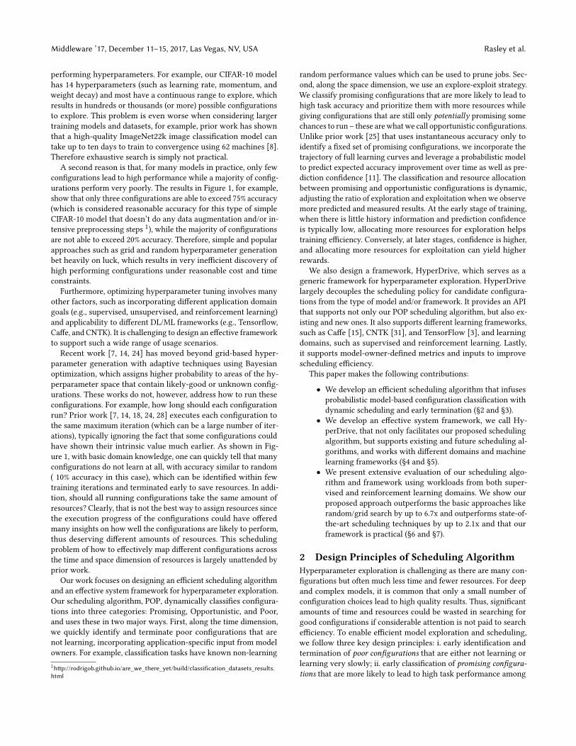
7.1 SimulatorOur goal is to compare the scheduling efficiency (i.e., time to reachtarget accuracy) between different policies under different resourcecapacities and configuration orders. We develop a trace-drivensimulator consisting of the following three main components, seeFigure 11:

• Trace Generator collects the traces from live system ex-periments and creates a replayable workload that containsiteration timing and performance metrics. In addition, theTrace Generator can create traces by changing the configu-ration orders. This feature is useful to conduct sensitivityanalysis of configuration orders.


• Simulator Engine is a trace-driven discrete event simula-tor that accurately emulates the execution process of Hy-perDrive, i.e., the order of configurations and the resourcemanagement logic.

• Pluggable Scheduling Policy dictates the scheduling de-cisions on configuration ordering and the resources allo-cated to different configurations over time.

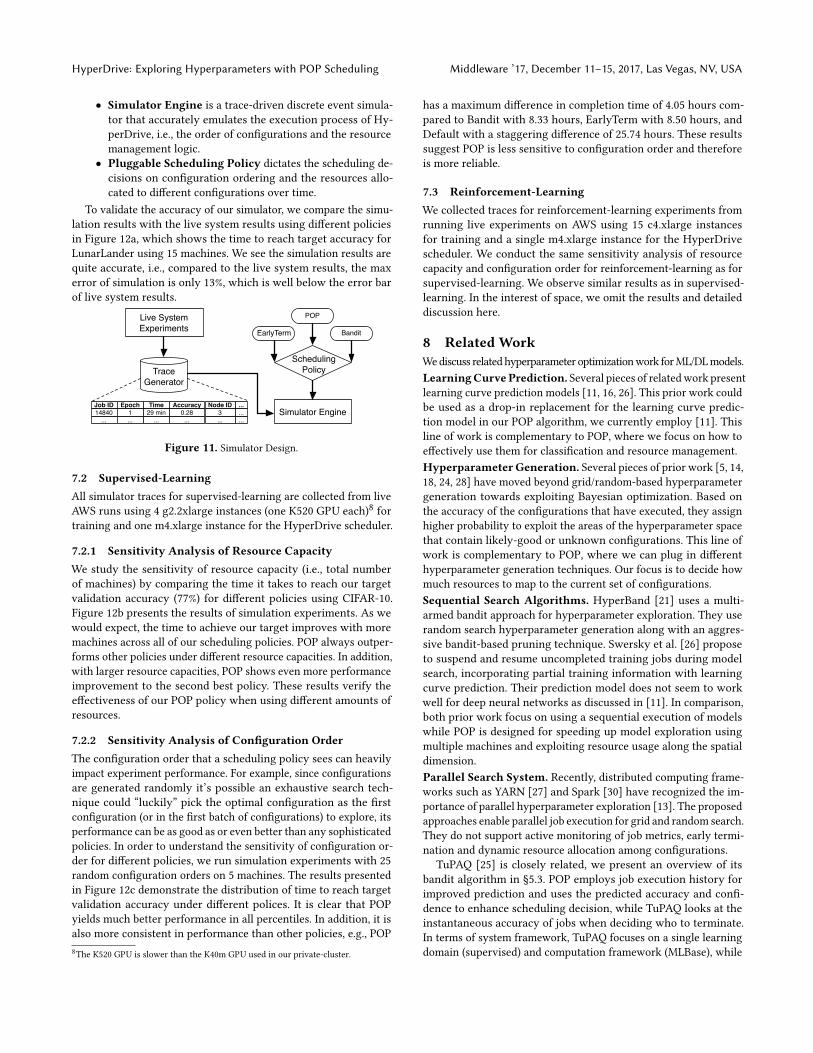
To validate the accuracy of our simulator, we compare the simu-lation results with the live system results using different policiesin Figure 12a, which shows the time to reach target accuracy forLunarLander using 15 machines. We see the simulation results arequite accurate, i.e., compared to the live system results, the maxerror of simulation is only 13%, which is well below the error barof live system results.

Trace Generator

Job ID

...14840

Epoch

...1

Time

...29 min

Accuracy

...0.28

Node ID

...3

...

...

...

Live System Experiments

Simulator Engine

EarlyTerm

Scheduling Policy

POP

Bandit

Figure 11. Simulator Design.

7.2 Supervised-LearningAll simulator traces for supervised-learning are collected from liveAWS runs using 4 g2.2xlarge instances (one K520 GPU each)8 fortraining and one m4.xlarge instance for the HyperDrive scheduler.

7.2.1 Sensitivity Analysis of Resource CapacityWe study the sensitivity of resource capacity (i.e., total numberof machines) by comparing the time it takes to reach our targetvalidation accuracy (77%) for different policies using CIFAR-10.Figure 12b presents the results of simulation experiments. As wewould expect, the time to achieve our target improves with moremachines across all of our scheduling policies. POP always outper-forms other policies under different resource capacities. In addition,with larger resource capacities, POP shows even more performanceimprovement to the second best policy. These results verify theeffectiveness of our POP policy when using different amounts ofresources.

7.2.2 Sensitivity Analysis of Configuration OrderThe configuration order that a scheduling policy sees can heavilyimpact experiment performance. For example, since configurationsare generated randomly it’s possible an exhaustive search tech-nique could “luckily” pick the optimal configuration as the firstconfiguration (or in the first batch of configurations) to explore, itsperformance can be as good as or even better than any sophisticatedpolicies. In order to understand the sensitivity of configuration or-der for different policies, we run simulation experiments with 25random configuration orders on 5 machines. The results presentedin Figure 12c demonstrate the distribution of time to reach targetvalidation accuracy under different polices. It is clear that POPyields much better performance in all percentiles. In addition, it isalso more consistent in performance than other policies, e.g., POP8The K520 GPU is slower than the K40m GPU used in our private-cluster.

has a maximum difference in completion time of 4.05 hours com-pared to Bandit with 8.33 hours, EarlyTerm with 8.50 hours, andDefault with a staggering difference of 25.74 hours. These resultssuggest POP is less sensitive to configuration order and thereforeis more reliable.

7.3 Reinforcement-LearningWe collected traces for reinforcement-learning experiments fromrunning live experiments on AWS using 15 c4.xlarge instancesfor training and a single m4.xlarge instance for the HyperDrivescheduler. We conduct the same sensitivity analysis of resourcecapacity and configuration order for reinforcement-learning as forsupervised-learning. We observe similar results as in supervised-learning. In the interest of space, we omit the results and detaileddiscussion here.

8 Related WorkWediscuss related hyperparameter optimizationwork forML/DLmodels.LearningCurvePrediction. Several pieces of relatedwork presentlearning curve prediction models [11, 16, 26]. This prior work couldbe used as a drop-in replacement for the learning curve predic-tion model in our POP algorithm, we currently employ [11]. Thisline of work is complementary to POP, where we focus on how toeffectively use them for classification and resource management.Hyperparameter Generation. Several pieces of prior work [5, 14,18, 24, 28] have moved beyond grid/random-based hyperparametergeneration towards exploiting Bayesian optimization. Based onthe accuracy of the configurations that have executed, they assignhigher probability to exploit the areas of the hyperparameter spacethat contain likely-good or unknown configurations. This line ofwork is complementary to POP, where we can plug in differenthyperparameter generation techniques. Our focus is to decide howmuch resources to map to the current set of configurations.Sequential Search Algorithms. HyperBand [21] uses a multi-armed bandit approach for hyperparameter exploration. They userandom search hyperparameter generation along with an aggres-sive bandit-based pruning technique. Swersky et al. [26] proposeto suspend and resume uncompleted training jobs during modelsearch, incorporating partial training information with learningcurve prediction. Their prediction model does not seem to workwell for deep neural networks as discussed in [11]. In comparison,both prior work focus on using a sequential execution of modelswhile POP is designed for speeding up model exploration usingmultiple machines and exploiting resource usage along the spatialdimension.Parallel Search System. Recently, distributed computing frame-works such as YARN [27] and Spark [30] have recognized the im-portance of parallel hyperparameter exploration [13]. The proposedapproaches enable parallel job execution for grid and random search.They do not support active monitoring of job metrics, early termi-nation and dynamic resource allocation among configurations.

TuPAQ [25] is closely related, we present an overview of itsbandit algorithm in §5.3. POP employs job execution history forimproved prediction and uses the predicted accuracy and confi-dence to enhance scheduling decision, while TuPAQ looks at theinstantaneous accuracy of jobs when deciding who to terminate.In terms of system framework, TuPAQ focuses on a single learningdomain (supervised) and computation framework (MLBase), while


�

��

��

��

��

��

��

��

��

(a) Simulator validation (LunarLander).

��

� ��

��

��

��

(b) Resource capacities (CIFAR-10).

��

�

� ��

��

��

��

��

(c) Random job orderings (CIFAR-10).Figure 12. Sensitivity analysis via simulation.

HyperDrive is designed as a comprehensive framework supportingdifferent algorithms across frameworks and domains. For perfor-mance, our evaluation results (in §6 and §7) show POP consistentlyout-performs our Bandit policy, which is based on TuPAQ.

9 DiscussionEpoch durations. Our POP policy assumes epoch durations re-main relatively constant during training (see §3.1.1). Epoch dura-tions may differ between unique sets of hyperparameter valuesbut for a specific configuration this duration remains relativelyconstant. This behavior is common in learning domains evaluatedin this work (supervised and reinforcement), however we leaveevaluating other domains that may experience non-constant epochdurations (e.g., genetic algorithms) to future work.Learning curve prediction. Our POP policy relies on a learningcurve prediction model. In this paper, we choose the model pro-posed in prior work [11] (which has been studied with extensiveevaluation) for this component, we have found it to work well forthe workloads we are using. In addition, we design the learningcurve prediction module as a pluggable component of HyperDrive,so users can easily switch to other prediction methods as preferred.Learning curve prediction is an active area of research [11, 16, 26]and we foresee no issue using different approaches as researchadvances in this area.User inputs.Our POP policy aims to achieve a training goal withinspecific time/resource constraints, therefore it requires as input amaximum experiment time (Tmax) and target performance (ytarget).SpecifyingTmax requires some knowledge related to typical configu-ration training time, since a too smallTmax may result in insufficienttime to finish model training. Setting ytarget is natural for domainswith known goals, such as our LunarLander task (see §6.3). How-ever, if a ytarget is unknown we have successfully used a dynamictarget approach to automatically adjust ytarget by gradually increas-ing the target once it is reached. In the interest of space, we leavethe details and evaluation of this approach to future work. In ourwork with practitioners we have found that before starting hyper-parameter exploration for their model they have a good idea aboutboth of POP’s required inputs.

POP, Bandit, and EarlyTerm policies all require a user-definedevaluation boundary (b) to be specified. Setting this value is acommon problem in the space of early-termination policies. Likein prior work, b is model/domain specific and should reflect thetime it takes to compute model performance and how long a useris willing to let a configuration execute before possible termination.We have found success with a heuristic of setting b to be between5-10% of the max epoch for a job. We leave automatically settingthis parameter to future work.

Ongoing Work. HyperDrive enables model owners to scheduleresources based on monitored application-level metrics. Typicallythere is a primary metric being optimized (e.g., accuracy) which iswhat POP utilizes. However, additionalmetrics of concern can be im-pacted by hyperparameter choices aswell, such as inference/servinglatencies, model sparsity/compressibility, etc.

We have seen promising early results exploring hyperparametersspecific to models that use Long Short-Term Memory (LSTM) units.We are working together with authors of recent work on improv-ing CNN model sparsity [29]. The work aims to reduce the size ofLSTMs structurally, for both storage saving and computation timesaving, without perplexity loss (the primary metric for our task).This is done through the use of group Lasso regularization [32],which adds enforcement on each group of a model’s weights. Themethod uses a new hyperparameter (i.e., λ) which makes a trade-offbetween sparsity and model perplexity. We have evaluated severalstate-of-the-art models from recent work [23, 33] with a newHyper-Drive policy, exploring λ values (plus other hyperparameters) whilemonitoring both perplexity and a sparsity-related metric. We haveseen significantly reduced training times by enabling user-definedglobal termination criteria through HyperDrive’s SAP API.

Lastly, we are working with Microsoft engineers to produc-tize HyperDrive internally, which will continue improving Hy-perDrive’s usability, scalability, and effectiveness. Hyperparameterexploration will continue to be an active research area but currentlythere are limited options to develop/evaluate parallel approachesthat incorporate techniques along both hyperparameter generationand scheduling (e.g., early termination, suspend/resume).

10 ConclusionThis paper presents an approach for improving the efficiency ofdeveloping machine learning models by optimizing hyperparame-ter exploration. Our approach includes two techniques: (i) the POPscheduling algorithm and (ii) the HyperDrive framework. POP em-ploys dynamic classification of model configurations and prioritizedresource scheduling to discover high-quality models faster thanstate-of-the-art approaches. HyperDrive is a flexible frameworkthat enables convenient evaluation of different hyperparameterexploration algorithms to improve the productivity of practitioners.We present experimental results that demonstrate the performancebenefits of using POP and HyperDrive to develop high-qualitymodels in supervised and reinforcement learning domains.

Acknowledgements:We thank our shepherd, Marco Canini, andanonymous reviewers for their valuable comments; those at Mi-crosoft helping to productize HyperDrive, Radu Kopetz, PrasanthPulavarthi, Sherlock Huang, Yue-Sheng Liu; Kavosh Asadi for provid-ing the RLmodel; earlyHyperDrive usersMinjia Zhang andWeiWen;Trishul Chilimbi for supporting the initial effort and brainstorming.


References[1] 2017. A high performance, open-source universal RPC framework. https://grpc.io.

(2017).[2] 2017. Checkpoint/Restore In Userspace (CRIU). https://criu.org/. (2017). Accessed:

2017-09-13.[3] Martín Abadi, Paul Barham, Jianmin Chen, Zhifeng Chen, Andy Davis, Jef-

frey Dean, Matthieu Devin, Sanjay Ghemawat, Geoffrey Irving, Michael Is-ard, Manjunath Kudlur, Josh Levenberg, Rajat Monga, Sherry Moore, Derek G.Murray, Benoit Steiner, Paul Tucker, Vijay Vasudevan, Pete Warden, MartinWicke, Yuan Yu, and Xiaoqiang Zheng. 2016. TensorFlow: A System for Large-Scale Machine Learning. In 12th USENIX Symposium on Operating Systems De-sign and Implementation (OSDI 16). USENIX Association, GA, 265–283. https://www.usenix.org/conference/osdi16/technical-sessions/presentation/abadi

[4] Kavosh Asadi and Jason D. Williams. 2016. Sample-efficient Deep ReinforcementLearning for Dialog Control. CoRR abs/1612.06000 (2016). http://arxiv.org/abs/1612.06000

[5] The GPyOpt authors. 2016. GPyOpt: A Bayesian Optimization framework inpython. http://github.com/SheffieldML/GPyOpt. (2016).

[6] James Bergstra, Olivier Breuleux, Frédéric Bastien, Pascal Lamblin, Razvan Pas-canu, Guillaume Desjardins, Joseph Turian, David Warde-Farley, and YoshuaBengio. 2010. Theano: A CPU and GPUMath Compiler in Python . In Proceedingsof the 9th Python in Science Conference, Stéfan van der Walt and Jarrod Millman(Eds.). 3 – 10.

[7] J. Bergstra, D. Yamins, and D. D. Cox. 2013. Making a Science of Model Search:Hyperparameter Optimization in Hundreds of Dimensions for Vision Archi-tectures. In Proceedings of the 30th International Conference on InternationalConference on Machine Learning - Volume 28 (ICML’13). JMLR.org, I–115–I–123.http://dl.acm.org/citation.cfm?id=3042817.3042832

[8] Trishul Chilimbi, Yutaka Suzue, Johnson Apacible, and Karthik Kalyanaraman.2014. Project Adam: Building an Efficient and Scalable Deep Learning TrainingSystem. In 11th USENIX Symposium on Operating Systems Design and Imple-mentation (OSDI 14). USENIX Association, Broomfield, CO, 571–582. https://www.usenix.org/conference/osdi14/technical-sessions/presentation/chilimbi

[9] François Chollet. 2015. Keras. https://github.com/fchollet/keras. (2015).[10] Ronan Collobert, Samy Bengio, and Johnny Mariéthoz. 2002. Torch: A Modular

Machine Learning Software Library. Idiap-RR Idiap-RR-46-2002. IDIAP.[11] Tobias Domhan, Jost Tobias Springenberg, and Frank Hutter. 2015. Speed-

ing Up Automatic Hyperparameter Optimization of Deep Neural Networksby Extrapolation of Learning Curves. In Proceedings of the 24th InternationalConference on Artificial Intelligence (IJCAI’15). AAAI Press, 3460–3468. http://dl.acm.org/citation.cfm?id=2832581.2832731

[12] Eyal Even-Dar, Shie Mannor, and Yishay Mansour. 2006. Action Elimination andStopping Conditions for the Multi-Armed Bandit and Reinforcement LearningProblems. Journal of machine learning research 7, Jun (2006), 1079–1105.

[13] Tim Hunter. 2016. Deep Learning with Apache Sparkand TensorFlow. https://databricks.com/blog/2016/01/25/deep-learning-with-apache-spark-and-tensorflow.html. (January 2016).

[14] F. Hutter, H. H. Hoos, and K. Leyton-Brown. 2011. Sequential Model-Based Opti-mization for General Algorithm Configuration. In Proc. of LION-5. 507âĂŞ523.

[15] Yangqing Jia, Evan Shelhamer, Jeff Donahue, Sergey Karayev, Jonathan Long,Ross Girshick, Sergio Guadarrama, and Trevor Darrell. 2014. Caffe: ConvolutionalArchitecture for Fast Feature Embedding. arXiv preprint arXiv:1408.5093 (2014).

[16] Aaron Klein, Stefan Falkner, Jost Tobias Springenberg, and Frank Hutter. 2017.Learning curve prediction with Bayesian neural networks. Proc. of ICLR 17(2017).

[17] Oleg Klimov. 2017. LunarLander-v2. https://gym.openai.com/envs/LunarLander-v2. (2017).

[18] Brent Komer, James Bergstra, and Chris Eliasmith. 2014. Hyperopt-sklearn:automatic hyperparameter configuration for scikit-learn. In ICML workshop onAutoML.

[19] Alex Krizhevsky. 2017. cuda-convnet. https://code.google.com/p/cuda-convnet/.(2017).

[20] Alex Krizhevsky and Geoffrey Hinton. 2009. Learning multiple layers of featuresfrom tiny images. (2009). Technical report, University of Toronto.

[21] Lisha Li, Kevin Jamieson, Giulia DeSalvo, Afshin Rostamizadeh, and AmeetTalwalkar. 2017. Hyperband: Bandit-based Configuration Evaluation for Hyper-parameter Optimization. Proc. of ICLR 17 (2017).

[22] Benjamin Recht, Christopher Re, Stephen Wright, and Feng Niu. 2011. Hogwild:A Lock-Free Approach to Parallelizing Stochastic Gradient Descent. In Advancesin Neural Information Processing Systems 24, J. Shawe-Taylor, R. S. Zemel, P. L.Bartlett, F. Pereira, and K. Q.Weinberger (Eds.). Curran Associates, Inc., 693–701.

[23] Min Joon Seo, Aniruddha Kembhavi, Ali Farhadi, and Hannaneh Hajishirzi.2016. Bidirectional Attention Flow for Machine Comprehension. arXiv CoRRabs/1611.01603 (2016). http://arxiv.org/abs/1611.01603

[24] Jasper Snoek, Hugo Larochelle, and Ryan P Adams. 2012. Practical bayesianoptimization of machine learning algorithms. In Advances in neural informationprocessing systems. 2951–2959.

[25] Evan R. Sparks, Ameet Talwalkar, Daniel Haas, Michael J. Franklin, Michael I.Jordan, and Tim Kraska. Automating Model Search for Large Scale MachineLearning. In Proceedings of the Sixth ACM Symposium on Cloud Computing (SoCC2015). 13. DOI:https://doi.org/10.1145/2806777.2806945

[26] Kevin Swersky, Jasper Snoek, and Ryan Prescott Adams. 2014. Freeze-ThawBayesian Optimization. arXiv preprint arXiv:1406.3896 (2014).

[27] Wangda Tan and Vinod Kumar Vavilapalli. 2017. Distributed Tensor-Flow Assembly on Apache Hadoop YARN. https://hortonworks.com/blog/distributed-tensorflow-assembly-hadoop-yarn/. (March 2017).

[28] Chris Thornton, Frank Hutter, Holger H. Hoos, and Kevin Leyton-Brown. 2013.Auto-WEKA: Combined Selection and Hyperparameter Optimization of Clas-sification Algorithms. In Proceedings of the 19th ACM SIGKDD InternationalConference on Knowledge Discovery and Data Mining (KDD ’13). ACM, New York,NY, USA, 847–855. DOI:https://doi.org/10.1145/2487575.2487629

[29] Wei Wen, Chunpeng Wu, Yandan Wang, Yiran Chen, and Hai Li. 2016. LearningStructured Sparsity in Deep Neural Networks. In Advances in Neural InformationProcessing Systems 29, D. D. Lee, M. Sugiyama, U. V. Luxburg, I. Guyon, andR. Garnett (Eds.). Curran Associates, Inc., 2074–2082. http://papers.nips.cc/paper/6504-learning-structured-sparsity-in-deep-neural-networks.pdf

[30] Lee Yang, Jun Shi, Bobbie Chern, and Andy Feng. 2017. OpenSourcing TensorFlowOnSpark: Distributed Deep Learning on Big-Data Clusters. http://yahoohadoop.tumblr.com/post/157196317141/open-sourcing-tensorflowonspark-distributed-deep. (February 2017).

[31] Dong Yu, Adam Eversole, Mike Seltzer, Kaisheng Yao, Oleksii Kuchaiev, YuZhang, Frank Seide, Zhiheng Huang, Brian Guenter, Huaming Wang, JashaDroppo, Geoffrey Zweig, Chris Rossbach, Jie Gao, Andreas Stolcke, Jon Currey,Malcolm Slaney, Guoguo Chen, Amit Agarwal, Chris Basoglu, Marko Padmilac,Alexey Kamenev, Vladimir Ivanov, Scott Cypher, Hari Parthasarathi, BhaskarMitra, Baolin Peng, and Xuedong Huang. 2014. An Introduction to ComputationalNetworks and the Computational Network Toolkit. Technical Report.

[32] Ming Yuan and Yi Lin. 2006. Model selection and estimation in regression withgrouped variables. Journal of the Royal Statistical Society: Series B (StatisticalMethodology) 68, 1 (2006), 49–67.

[33] Wojciech Zaremba, Ilya Sutskever, and Oriol Vinyals. 2014. Recurrent NeuralNetwork Regularization. arXiv CoRR abs/1409.2329 (2014). http://arxiv.org/abs/1409.2329

https://grpc.io

https://criu.org/

https://www.usenix.org/conference/osdi16/technical-sessions/presentation/abadi

https://www.usenix.org/conference/osdi16/technical-sessions/presentation/abadi

http://arxiv.org/abs/1612.06000


http://github.com/SheffieldML/GPyOpt

http://dl.acm.org/citation.cfm?id=3042817.3042832

https://www.usenix.org/conference/osdi14/technical-sessions/presentation/chilimbi

https://www.usenix.org/conference/osdi14/technical-sessions/presentation/chilimbi

https://github.com/fchollet/keras



https://databricks.com/blog/2016/01/25/deep-learning-with-apache-spark-and-tensorflow.html

https://databricks.com/blog/2016/01/25/deep-learning-with-apache-spark-and-tensorflow.html

https://gym.openai.com/envs/LunarLander-v2

https://gym.openai.com/envs/LunarLander-v2

https://code.google.com/p/cuda-convnet/


https://doi.org/10.1145/2806777.2806945

https://hortonworks.com/blog/distributed-tensorflow-assembly-hadoop-yarn/

https://hortonworks.com/blog/distributed-tensorflow-assembly-hadoop-yarn/

https://doi.org/10.1145/2487575.2487629

http://papers.nips.cc/paper/6504-learning-structured-sparsity-in-deep-neural-networks.pdf

http://papers.nips.cc/paper/6504-learning-structured-sparsity-in-deep-neural-networks.pdf

http://yahoohadoop.tumblr.com/post/157196317141/open-sourcing-tensorflowonspark-distributed-deep

http://yahoohadoop.tumblr.com/post/157196317141/open-sourcing-tensorflowonspark-distributed-deep



hyperdrive: exploring hyperparameters with pop scheduling · 2018-05-24 · hyperdrive: exploring...

Documents