Hyperbolic isomorphismsin Banach spaces

Jose Ferreira Alves

June 24, 2014

Contents

Introduction ii

1 Bounded linear operators 1

2 Spectrum and resolvent 3

3 Spectral decomposition 7

4 Complexification 11

5 Hyperbolic isomorphisms 14

6 Structural stability 19

7 Open problem 27

8 Exercises 27

References 29

i

Introduction

The main goal of these notes is to generalize some results which are standard for linear iso-morphisms of finite dimensional vector spaces to infinite dimensional spaces. In particular,we shall prove that there exists an invariant splitting for any hyperbolic bounded linearisomorphism on a Banach space and that such an isomorphism is structurally stable.

Let us start with some motivational considerations in the finite dimensional setting.Consider A : E → E an isomorphism of a vector space E over R or C with finite dimension.It is well known that by a suitable choice of a basis in E the isomorphism A can berepresented by a block diagonal matrix

J =

J1. . .

Jn

,

where each Ji is a Jordan block. In the complex case, by a Jordan block we mean a squarematrix of the form

Ji =

λi 1

λi. . .. . . 1

λi

, (?)

where each λi is an eigenvalue of A. In the real case, a Jordan block can either be a matrixof the type (?), corresponding to a real eigenvalue λi of A, or a matrix

Ji =

Ci I

Ci. . .. . . I

Ci

,

where

Ci =

(ai bi−bi ai

)and I =

(1 00 1

),

corresponding to a complex eigenvalue λi = ai + ibi with bi 6= 0. In this last case, by aneigenvalue of A we mean a root of the characteristic polynomial of A. We leave it as anexercise to show that:

1. if e1, . . . , em are vectors in a basis associated to a Jordan block of an eigenvalue λ ofA with |λ| < 1, then Anx→ 0 as n→ +∞ for all x ∈ span{e1, . . . , em};

2. if f1, . . . , fn are vectors in a basis associated to a Jordan block of an eigenvalue λ ofA with |λ| > 1, then A−nx→ 0 as n→ +∞ for all x ∈ span{f1, . . . , fn}.

ii

Hence, if A has no eigenvalues in the unit circle, then there are subspaces Es andEu of E (called the stable and unstable spaces of A, respectively) for which the followingproperties hold:

1. E = Es ⊕ Eu;

2. Anx→ 0 as n→ +∞ for all x ∈ Es;

3. A−nx→ 0 as n→ +∞ for all x ∈ Eu.

As a linear isomorphism of an infinite dimensional Banach space may have no eigenval-ues we need an alternative method to find the stable and unstable spaces. The idea is toconsider the more general notion of spectrum of an operator and the projections associatedto certain isolated parts of the spectrum.

We shall try to make these notes as self-contained as possible, in particular provingmost of the results we need from Functional Analysis and Spectral Theory. In Sections 1and 2 we consider some basic results on bounded linear operators. We introduce thenotion of spectrum of a bounded linear operator and prove some of its basic properties. InSection 3 we prove a Spectral Decomposition Theorem for operators whose spectrum canbe decomposed into two isolated parts.

The results in Sections 2 and 3 are specific for complex Banach spaces. In order toobtain our conclusions on the dynamics of hyperbolic linear isomorphisms in the real caseas well, in Section 4 we recall the standard notion of complexification, both of a real vectorspace and of an operator defined on that real space. In particular, we shall introduce asuitable norm in the complexification space.

In Section 5 we apply the Spectral Decomposition Theorem to an operator whosespectrum is disjoint from the unit circle, both in the complex and real cases, and obtainfor a linear isomorphisms of a Banach space the decomposition of that space into a directsum of sable an unstable spaces. This depicts a fairly reasonable scenario for the dynamicsof such hyperbolic isomorphisms.

Another important issue in Dynamical Systems Theory is the structural stability of asystem, meaning that the dynamics is not affected under a small perturbation of the system.We shall also address this question for isomorphisms of infinite dimensional spaces. InSection 6 we prove that a hyperbolic linear isomorphism of a Banach space is topologicallyconjugate to any nearby isomorphism.

iii

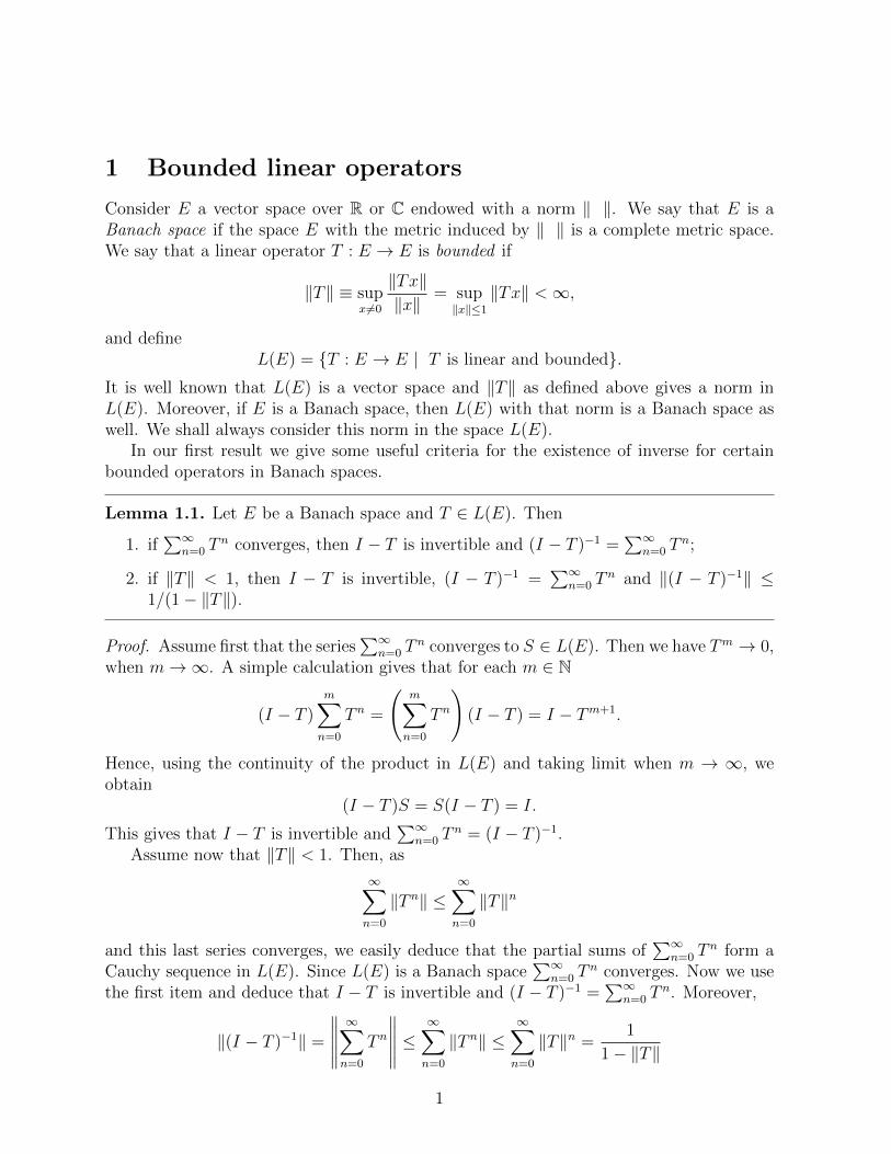
1 Bounded linear operators

Consider E a vector space over R or C endowed with a norm ‖ ‖. We say that E is aBanach space if the space E with the metric induced by ‖ ‖ is a complete metric space.We say that a linear operator T : E → E is bounded if

‖T‖ ≡ supx 6=0

‖Tx‖‖x‖

= sup‖x‖≤1

‖Tx‖ <∞,

and defineL(E) = {T : E → E | T is linear and bounded}.

It is well known that L(E) is a vector space and ‖T‖ as defined above gives a norm inL(E). Moreover, if E is a Banach space, then L(E) with that norm is a Banach space aswell. We shall always consider this norm in the space L(E).

In our first result we give some useful criteria for the existence of inverse for certainbounded operators in Banach spaces.

Lemma 1.1. Let E be a Banach space and T ∈ L(E). Then

1. if∑∞

n=0 Tn converges, then I − T is invertible and (I − T )−1 =

∑∞n=0 T

n;

2. if ‖T‖ < 1, then I − T is invertible, (I − T )−1 =∑∞

n=0 Tn and ‖(I − T )−1‖ ≤

1/(1− ‖T‖).

Proof. Assume first that the series∑∞

n=0 Tn converges to S ∈ L(E). Then we have Tm → 0,

when m→∞. A simple calculation gives that for each m ∈ N

(I − T )m∑n=0

T n =

(m∑n=0

T n

)(I − T ) = I − Tm+1.

Hence, using the continuity of the product in L(E) and taking limit when m → ∞, weobtain

(I − T )S = S(I − T ) = I.

This gives that I − T is invertible and∑∞

n=0 Tn = (I − T )−1.

Assume now that ‖T‖ < 1. Then, as

∞∑n=0

‖T n‖ ≤∞∑n=0

‖T‖n

and this last series converges, we easily deduce that the partial sums of∑∞

n=0 Tn form a

Cauchy sequence in L(E). Since L(E) is a Banach space∑∞

n=0 Tn converges. Now we use

the first item and deduce that I − T is invertible and (I − T )−1 =∑∞

n=0 Tn. Moreover,

‖(I − T )−1‖ =

∥∥∥∥∥∞∑n=0

T n

∥∥∥∥∥ ≤∞∑n=0

‖T n‖ ≤∞∑n=0

‖T‖n =1

1− ‖T‖

1

for ‖T‖ < 1. tu

As illustrated in the introduction, the existence of stable and unstable spaces for anisomorphism on a finite dimensional space can be obtained knowing the eigenvalues ofthe isomorphism and the corresponding generalized eigenspaces. As eigenvalues of anisomorphism of an infinite dimensional space need not to exist in general, the idea is toconsider the more general notion of spectrum of an operator and the projections associatedto certain isolated parts of that spectrum.

Definition 1.2. We say that a bounded linear operator P : E → E of a vector space E isa projection if P 2 = P .

In the next result we give some useful properties of projections. By I : E → E wemean the identity operator in the vector space E.

Proposition 1.3. Let P : E → E be a projection. Then:

1. I − P is a projection;

2. P (E) = ker(I − P );

3. P (E) is a closed subspace of E;

4. E = P (E)⊕ (I − P )(E).

Proof. 1. A simple calculation gives

(I − P )2 = (I − P )(I − P ) = I − P − P + P 2 = I − P,

where this last equality follows form the fact that P is a projection.2. If y = Px for some x ∈ E, then y − Py = Px − P 2x = Px − Px = 0. Hence,

y ∈ ker(I − P ). On the other hand, if y ∈ ker(I − P ), then y = Py, and so y ∈ P (E).3. Since P (E) = ker(I − P ) by the second item, then we have P (E) = (I − P )−1{0}

where {0} is a closed set and I − P is continuous. Therefore P (E) is a closed subspace.4. Given x ∈ E, we may write x = Px + (I − P )x. It remains to prove that P (E) ∩

(I − P )(E) = {0}. Given x ∈ P (E) ∩ (I − P )(E), there are y, z ∈ E such that x = Pyand x = z−Pz. We have in particular Py = z−Pz. Applying P to both sides, we obtainP 2y = Pz − P 2z. As P is a projection, we have Py = z − Pz = 0 and this implies thatx = 0. tu

2

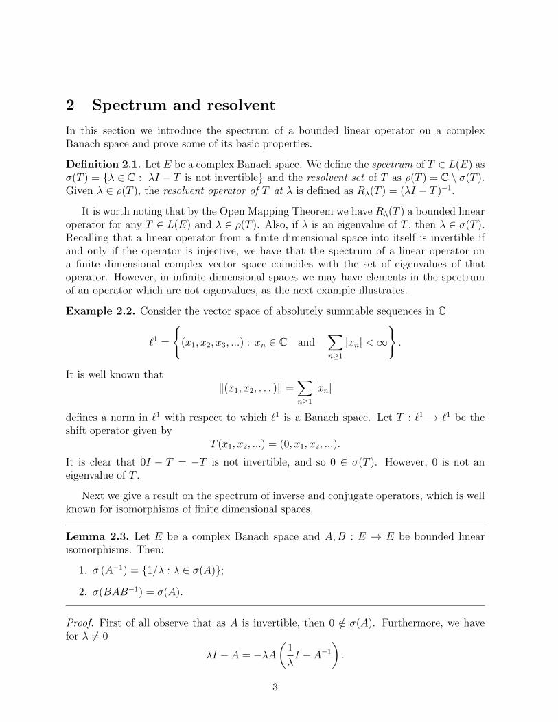
2 Spectrum and resolvent

In this section we introduce the spectrum of a bounded linear operator on a complexBanach space and prove some of its basic properties.

Definition 2.1. Let E be a complex Banach space. We define the spectrum of T ∈ L(E) asσ(T ) = {λ ∈ C : λI − T is not invertible} and the resolvent set of T as ρ(T ) = C \ σ(T ).Given λ ∈ ρ(T ), the resolvent operator of T at λ is defined as Rλ(T ) = (λI − T )−1.

It is worth noting that by the Open Mapping Theorem we have Rλ(T ) a bounded linearoperator for any T ∈ L(E) and λ ∈ ρ(T ). Also, if λ is an eigenvalue of T , then λ ∈ σ(T ).Recalling that a linear operator from a finite dimensional space into itself is invertible ifand only if the operator is injective, we have that the spectrum of a linear operator ona finite dimensional complex vector space coincides with the set of eigenvalues of thatoperator. However, in infinite dimensional spaces we may have elements in the spectrumof an operator which are not eigenvalues, as the next example illustrates.

Example 2.2. Consider the vector space of absolutely summable sequences in C

`1 =

{(x1, x2, x3, ...) : xn ∈ C and

∑n≥1

|xn| <∞

}.

It is well known that‖(x1, x2, . . . )‖ =

∑n≥1

|xn|

defines a norm in `1 with respect to which `1 is a Banach space. Let T : `1 → `1 be theshift operator given by

T (x1, x2, ...) = (0, x1, x2, ...).

It is clear that 0I − T = −T is not invertible, and so 0 ∈ σ(T ). However, 0 is not aneigenvalue of T .

Next we give a result on the spectrum of inverse and conjugate operators, which is wellknown for isomorphisms of finite dimensional spaces.

Lemma 2.3. Let E be a complex Banach space and A,B : E → E be bounded linearisomorphisms. Then:

1. σ (A−1) = {1/λ : λ ∈ σ(A)};

2. σ(BAB−1) = σ(A).

Proof. First of all observe that as A is invertible, then 0 /∈ σ(A). Furthermore, we havefor λ 6= 0

λI − A = −λA(

1

λI − A−1

).

3

Hence, if A ∈ GL(E), then λI −A is invertible if and only if I/λ−A−1 is invertible. Thisproves the first assertion.

Given B ∈ GL(E) and λ ∈ C, we may write

λI −BAB−1 = B(λI)B−1 −BAB−1 = B(λI − A)B−1.

Hence, λI −BAB−1 is invertible if and only if λI − A is invertible. tu

In the next result we consider analytic functions defined on some open set of the complexplane and taking values in a complex Banach space. Essentially all the main definitionsand results of the theory of complex valued functions, such as Contour Integrals, ResidueTheorem and Liouville Theorem, remain true in this more general context; see e.g. [1].

Theorem 2.4. Let E be a complex Banach space and T ∈ L(E). Then:

1. ρ(T ) is open in C and it contains {λ ∈ C : |λ| > ‖T‖};

2. Rλ(T ) =1

λ

∞∑n=0

T n

λnfor all |λ| > ‖T‖;

3. ρ(T ) 3 λ 7−→ Rλ(T ) ∈ L(E) is an analytic function.

Proof. If |λ| > ‖T‖, then using Lema 1.1 we easily deduce that λI − T is invertible and

Rλ(T ) =1

λ

(I − T

λ

)−1=

1

λ

∞∑n=0

T n

λn.

Thus we have proved that ρ(T ) ⊃ {λ ∈ C : |λ| > ‖T‖} and also the second item.Given λ0 ∈ ρ(T ), take λ ∈ C close enough to λ0 so that

|λ− λ0| · ‖Rλ0(T )‖ < 1. (1)

WritingλI − T = λ0I − T + (λ− λ0)I =

[I − (λ− λ0)Rλ0(T )

](λ0I − T ),

then Lemma 1.1 gives that λ ∈ ρ(T ) for λ satisfying (1), thus proving that ρ(T ) is an openset. Moreover,

Rλ(T ) = Rλ0(T ) [I − (λ− λ0)Rλ0(T )]−1 .

Now Lemma 1.1 gives that

[I − (λ− λ0)Rλ0(T )]−1 =∞∑n=0

(λ− λ0)nRλ0(T )n,

4

and so

Rλ(T ) = Rλ0(T )∞∑n=0

(λ− λ0)nRλ0(T )n.

Thus we have written Rλ(T ) as a convergent power series around λ0, thereby proving itsanalyticity. tu

This last theorem shows that∑∞

n=1 Tn−1/λn is the Laurent series of the function Rλ(T )

in the annulus {‖T‖ < |z| < ∞}. So we can use the theory of holomorphic functions todeduce many results about Rλ(T ) using this expansion. To start with, we consider a Jordancurve γ oriented counterclockwise and containing the disk {|z| ≤ ‖T‖} in its interior. TheResidue Theorem gives that

1

2πi

∫γ

Rλ(T )dλ = I.

Such utilization of curves and contour integrals to separate different parts of the spectrumwill be very useful in defining projection operators which will give a splitting into stableand unstable spaces of hyperbolic isomorphisms.

Theorem 2.5. Let E 6= {0} be a complex Banach space and T ∈ L(E). Then σ(T ) is anonempty compact set contained in {|z| ≤ ‖T‖}.

Proof. Noticing that σ(T ) = C \ ρ(T ), it immediately follows fromTheorem 2.4 that σ(T )is a closed set and σ(T ) ⊂ {z ∈ C : |z| ≤ ‖T‖}. It remains to see that σ(T ) is nonempty.Assume, by contradiction, that ρ(T ) = ∅. This implies that λ 7→ Rλ(T ) is an analyticfunction defined in the whole complex plane. Moreover, it follows from Lemma 1.1 thatfor |λ| > ‖T‖ we have

‖Rλ(T )‖ =

∥∥∥∥∥1

λ

(I − T

λ

)−1∥∥∥∥∥ ≤ 1

|λ|(1− ‖T/λ‖).

Thus, λ 7→ Rλ(T ) is a bounded function. Hence, by Liouville Theorem it must be constant.As Rλ(T ) → 0 when λ → ∞, it follows that Rλ(T ) = 0. This gives a contradiction forE 6= {0}. tu

Definition 2.6. Let E be a complex vector space. We define the spectral radius of anopreator T ∈ L(E) as

r(T ) = supλ∈σ(T )

|λ|.

5

Theorem 2.7. Let E be a complex Banach space and T ∈ L(E). Then

r(T ) = limn→∞

‖T n‖1/n = infn≥1‖T n‖1/n.

Proof. We start by showing that limn→∞ ‖T n‖1/n exists and coincides with

s(T ) = lim infn≥1

‖T n‖1/n.

For this, it is sufficient to show that

lim supn→+∞

‖T n‖1/n ≤ s(T ). (2)

Given an arbitrary ε > 0, fix p ∈ N such that ‖T p‖1/p < s(T ) + ε. Any n ∈ N can bewritten as n = pq+ r with 0 ≤ r < p. Then, using the fact that norm is submultiplicative,we obtain

‖T n‖1/n = ‖T pq+r‖1/n ≤ ‖T p‖q/n‖T‖r/n < (s(T ) + ε)pq/n‖T‖r/n.Since pq/n→ 1 and r/n→ 0 when n→ +∞, it follows that

lim supn→+∞

‖T n‖1/n ≤ s(T ) + ε.

Since ε > 0 is arbitrary, we have proved (2).Let us now prove that r(T ) ≤ s(T ), or equivalently, λ ∈ ρ(T ) for |λ| > s(T ). In fact,

taking c = |λ| − s(T ) > 0, we obtain ‖T n‖ < [s(T ) + c/2]n for sufficiently large n, sincelimn→+∞ ‖T n‖1/n = s(T ). Then,

1

|λ|n‖T n‖ ≤

(s(T ) + c/2

s(T ) + c

)n,

which shows that the series∑∞

n=0 Tn/λn converges in L(E). Moreover, by Lemma 1.1 we

can write1

λ

∞∑n=0

T n

λn=

1

λ

(I − T

λ

)−1= Rλ(T ), (3)

and so we have proved that λ ∈ ρ(T ) for |λ| > s(T ).It remains to show that r(T ) ≥ s(T ). Theorem 2.4 gives that r(T ) ≤ ‖T‖ and the

function λ 7→ Rλ(T ) is analytic for |λ| > r(T ). In particular, Rλ(T ) admits a Laurentseries representation centered at 0 for |λ| > r(T ). Equation (3) shows that this series isnecessarily

∑∞n=1 T

n−1/λn. Thus we have limn→∞ ‖λ−nT n‖ = 0 for any |λ| > r(T ). Hence,given an arbitrary ε > 0, we have ‖T n‖ ≤ [ε+ r(T )]n for n large. As ε > 0 is arbitrary, weobtain

s(T ) = limn→∞

‖T n‖1/n ≤ r(T ).

Thus we have proved that r(T ) = s(T ). tu

As r(T ) is obviously bounded by ‖T‖, equation (3) shows that the formula obtained inTheorem 2.4 can be extended to the annulus {λ ∈ C : r(T ) < |λ| <∞}.

6

3 Spectral decomposition

In the next result we show that if the spectrum of an operator on a complex Banac spacecan be split into two disjoint compact parts, then corresponding to such splitting in thespectrum there is a splitting in the space.

Theorem 3.1 (Spectral Decomposition). Let E be a complex Banach space and T ∈ L(E).Assume that σ(T ) = σ1 ∪σ2, where σ1, σ2 are compact disjoint sets. Then there are closedspaces E1, E2 with:

1. E = E1 ⊕ E2;

2. T (E1) ⊂ E1 and T (E2) ⊂ E2;

3. σ(T |E1) = σ1 and σ(T |E2) = σ2.

Proof. Assume that σ(T ) = σ1 ∪ σ2, where σ1, σ2 are compact and disjoint. Consider aJordan curve γ ⊂ ρ(T ) oriented counterclockwise, containing σ1 in its interior and σ2 inits exterior. We define the operator in L(E)

P1 =1

2πi

∫γ

Rλ(T )dλ.

Let γ′ be another Jordan curve oriented counterclockwise, containing γ in its interior andσ2 in its exterior. As γ and γ′ are homotopic in ρ(T ), we have

P1 =1

2πi

∫γ

Rλ(T )dλ =1

2πi

∫γ′Rλ′(T )dλ′.

Let us now prove that P1 is a projection. First of all observe that for λ, λ′ ∈ ρ(T ) we have

Rλ(T ) = Rλ(T )(λ′I − T )Rλ′(T )

= Rλ(T )[λI − T + (λ′ − λ)I

]Rλ′(T )

=[I + (λ′ − λ)Rλ(T )

]Rλ′(T )

= Rλ′(T ) + (λ′ − λ)Rλ(T )Rλ′(T ). (4)

Now, using (4) in the second equality below we may write

P 21 =

1

(2πi)2

∫γ

∫γ′Rλ(T )Rλ′(T )dλ′dλ

=1

(2πi)2

∫γ

∫γ′

Rλ(T )−Rλ′(T )

λ′ − λdλ′dλ

=1

(2πi)2

∫γ

∫γ′

Rλ(T )

λ′ − λdλ′dλ− 1

(2πi)2

∫γ

∫γ′

Rλ′(T )

λ′ − λdλ′dλ

=1

2πi

∫γ

Rλ(T )1

2πi

∫γ′

dλ′

λ′ − λdλ+

1

2πi

∫γ′Rλ′(T )

1

2πi

∫γ

dλ

λ− λ′dλ′.

7

Noting that we are taking γ inside γ′, we have for λ ∈ γ and λ′ ∈ γ′

1

2πi

∫γ′

dλ′

λ′ − λ= 1 and

1

2πi

∫γ

dλ

λ− λ′= 0,

from which we deduce that P 21 = P1, and so P1 is a projection.

Defining P2 = I − P1 and the spaces E1 = P1(E) and E2 = P2(E), we have byProposition 1.3 that E1 and E2 are closed subspaces and

E = E1 ⊕ E2.

Moreover, as T commutes with λI−T , we have that T commutes with Rλ(T ) for λ ∈ ρ(T ).Integrating we get

P1T = TP1.

Then we haveT (E1) = TP1(E) = P1T (E) ⊂ P1(E) = E1.

Similarly we see that T (E2) ⊂ E2, thus having proved the first two items of the theorem.Now we are going to see that

σ(T ) = σ(T |E1) ∪ σ(T |E2). (5)

It easily follows from (4) that for all λ, λ′ ∈ ρ(T ) we have

Rλ′(T )Rλ(T ) = Rλ(T )Rλ′(T ),

and so, integrating with respect to λ′ along the curve γ′, this yields

P1Rλ(T ) = Rλ(T )P1.

Hence(λI − T )P1Rλ(T ) = (λI − T )Rλ(T )P1 = P1. (6)

AlsoRλ(T )(λI − T )P1 = P1. (7)

Noticing that P1|E1 is the identity, restricting equalities (6) and (7) to E1 we deduce thatλ ∈ ρ(T |E1) and Rλ(T |E1) = Rλ(T )|E1 , thus proving that ρ(T ) ⊂ ρ(T |E1). Using that P2

commutes with Rλ(T ) as well, we also see that ρ(T ) ⊂ ρ(T |E2). Hence we have

ρ(T ) ⊂ ρ(T |E1) ∩ ρ(T |E2). (8)

Besides, as T (E1) ⊂ E1 and T (E2) ⊂ E2, we easily see that Rλ(T ) = Rλ(T |E1)⊕Rλ(T |E2)for λ ∈ ρ(T |E1) ∩ ρ(T |E2). This shows that ρ(T |E1) ∩ ρ(T |E2) ⊂ ρ(T ), which togetherwith (8) gives (5).

8

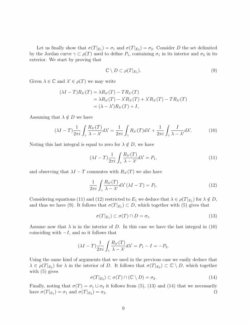
Let us finally show that σ(T |E1) = σ1 and σ(T |E2) = σ2. Consider D the set delimitedby the Jordan curve γ ⊂ ρ(T ) used to define P1, containing σ1 in its interior and σ2 in itsexterior. We start by proving that

C \D ⊂ ρ(T |E1). (9)

Given λ ∈ C and λ′ ∈ ρ(T ) we may write

(λI − T )Rλ′(T ) = λRλ′(T )− TRλ′(T )

= λRλ′(T )− λ′Rλ′(T ) + λ′Rλ′(T )− TRλ′(T )

= (λ− λ′)Rλ′(T ) + I,

Assuming that λ /∈ D we have

(λI − T )1

2πi

∫γ

Rλ′(T )

λ− λ′dλ′ =

1

2πi

∫γ

Rλ′(T )dλ′ +1

2πi

∫γ

I

λ− λ′dλ′. (10)

Noting this last integral is equal to zero for λ /∈ D, we have

(λI − T )1

2πi

∫γ

Rλ′(T )

λ− λ′dλ′ = P1, (11)

and observing that λI − T commutes with Rλ′(T ) we also have

1

2πi

∫γ

Rλ′(T )

λ− λ′dλ′ (λI − T ) = P1. (12)

Considering equations (11) and (12) restricted to E1 we deduce that λ ∈ ρ(T |E1) for λ /∈ D,and thus we have (9). It follows that σ(T |E1) ⊂ D, which together with (5) gives that

σ(T |E1) ⊂ σ(T ) ∩D = σ1. (13)

Assume now that λ is in the interior of D. In this case we have the last integral in (10)coinciding with −I, and so it follows that

(λI − T )1

2πi

∫γ

Rλ′(T )

λ− λ′dλ′ = P1 − I = −P2.

Using the same kind of arguments that we used in the previous case we easily deduce thatλ ∈ ρ(T |E2) for λ in the interior of D. It follows that σ(T |E2) ⊂ C \ D, which togetherwith (5) gives

σ(T |E2) ⊂ σ(T ) ∩ (C \D) = σ2. (14)

Finally, noting that σ(T ) = σ1 ∪ σ2 it follows from (5), (13) and (14) that we necessarilyhave σ(T |E1) = σ1 and σ(T |E2) = σ2. tu

9

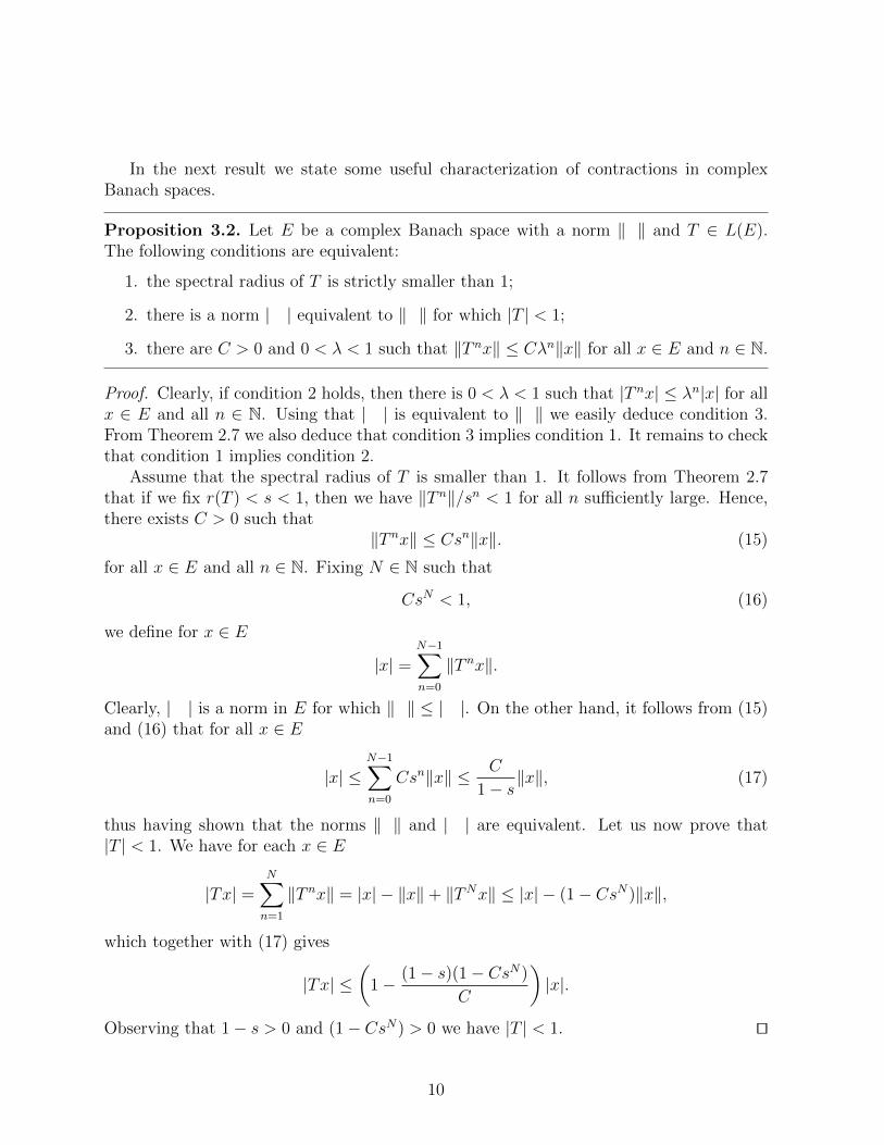
In the next result we state some useful characterization of contractions in complexBanach spaces.

Proposition 3.2. Let E be a complex Banach space with a norm ‖ ‖ and T ∈ L(E).The following conditions are equivalent:

1. the spectral radius of T is strictly smaller than 1;

2. there is a norm | | equivalent to ‖ ‖ for which |T | < 1;

3. there are C > 0 and 0 < λ < 1 such that ‖T nx‖ ≤ Cλn‖x‖ for all x ∈ E and n ∈ N.

Proof. Clearly, if condition 2 holds, then there is 0 < λ < 1 such that |T nx| ≤ λn|x| for allx ∈ E and all n ∈ N. Using that | | is equivalent to ‖ ‖ we easily deduce condition 3.From Theorem 2.7 we also deduce that condition 3 implies condition 1. It remains to checkthat condition 1 implies condition 2.

Assume that the spectral radius of T is smaller than 1. It follows from Theorem 2.7that if we fix r(T ) < s < 1, then we have ‖T n‖/sn < 1 for all n sufficiently large. Hence,there exists C > 0 such that

‖T nx‖ ≤ Csn‖x‖. (15)

for all x ∈ E and all n ∈ N. Fixing N ∈ N such that

CsN < 1, (16)

we define for x ∈ E

|x| =N−1∑n=0

‖T nx‖.

Clearly, | | is a norm in E for which ‖ ‖ ≤ | |. On the other hand, it follows from (15)and (16) that for all x ∈ E

|x| ≤N−1∑n=0

Csn‖x‖ ≤ C

1− s‖x‖, (17)

thus having shown that the norms ‖ ‖ and | | are equivalent. Let us now prove that|T | < 1. We have for each x ∈ E

|Tx| =N∑n=1

‖T nx‖ = |x| − ‖x‖+ ‖TNx‖ ≤ |x| − (1− CsN)‖x‖,

which together with (17) gives

|Tx| ≤(

1− (1− s)(1− CsN)

C

)|x|.

Observing that 1− s > 0 and (1− CsN) > 0 we have |T | < 1. tu

10

4 Complexification

Here we recall the well-know process of complexification of a real vector space and introducea useful norm in that complexification space. Given a real vector space E, define

EC = {x+ iy : x, y ∈ E}.

We introduce in EC a structure of complex vector space, defining the addition of x + iyand u+ iv in EC as

(x+ iy) + (u+ iv) = (x+ u) + i(y + v)

and the multiplication of α + iβ ∈ C by x+ iy ∈ EC as

(α + iβ)(x+ iy) = (αx− βy) + i(αy + βx).

We leave it as a straightforward exercise to verify that EC endowed with these operationshas a structure of complex vector space, called the complexification of E.

The problem of introducing a norm in EC for which EC inherits important propertiesfrom E (being a Banach space, for instance) is more subtle than it may appear at firstsight. An attempt to define a norm in the complexification space has been made by A. E.Taylor through

‖x+ iy‖C =√‖x‖2 + ‖y‖2

for each x + iy ∈ EC. The problem with ‖ ‖C is that in general it fails to have thehomogeneous property over the complex numbers. A reasonable norm has been proposedlater by A. E. Taylor, defining for each x+ iy ∈ EC

‖x+ iy‖C = supθ∈[0,2π]

‖ cos θ x− sin θ y‖. (18)

For many other considerations about possible choices of reasonable norms in complexifica-tion spaces see e.g. [6].

Proposition 4.1. If E be a real vector space with a norm ‖ ‖, then ‖ ‖C defined asin (18) gives a norm in EC such that for all x, y ∈ E

max{‖x‖, ‖y‖} ≤ ‖x+ iy‖C ≤ ‖x‖+ ‖y‖. (19)

Proof. Let us see first that for all x, y ∈ E we have (19). In fact, it easily follows from thedefinition of ‖ ‖C that for all x, y ∈ E

‖x‖ = ‖ cos 0x− sin 0 y‖ ≤ ‖x+ iy‖C

and‖y‖ =

∥∥∥cosπ

2x− sin

π

2y∥∥∥ ≤ ‖x+ iy‖C.

11

Furthermore, for each θ ∈ [0, 2π] we have

‖ cos θx− sin θy‖ ≤ | cos θ|‖x‖+ | sin θ|‖y‖ ≤ ‖x‖+ ‖y‖,

which finally gives (19).Let us now see that ‖ ‖C defines a norm in EC. From (19) we easily deduce that

‖x+ iy‖C = 0 ⇔ x = 0.

Moreover, given x, y ∈ E and λ ∈ C, choose α ∈ [0, 2π] such that λ = |λ|(cosα + i sinα).We have

‖λ(x+ iy)‖C = ‖|λ|(cosα + i sinα)(x+ iy)‖C= ‖|λ|[(cosαx− sinα y) + i(cosα y + sinαx)]‖C= |λ| sup

θ∈[0,2π]‖ cos θ(cosαx− sinα y)− sin θ(cosα y + sinαx)‖

= |λ| supθ∈[0,2π]

‖ cos(θ + α)x− sin(θ + α)y‖

= |λ| ‖x+ iy‖C,

and so we have the homogeneous property. Let us finally prove the triangular inequality.For u+ iv, x+ iy ∈ EC we have

‖(u+ iv) + (x+ iy)‖C = ‖(u+ x) + (v + y)i‖C= sup

θ∈[0,2π]‖ cos θ (u+ x)− sin θ (v + y)‖

= supθ∈[0,2π]

‖ cos θ u− sin θ v + cos θ x− sin θ y‖

≤ supθ∈[0,2π]

‖ cos θ u− sin θ v‖+ supθ∈[0,2π]

‖ cos θ x− sin θ y‖

= ‖u+ iv‖C + ‖x+ iy‖C,

which gives the triangular inequality. tu

From here on we shall always assume that ‖ ‖C related to ‖ ‖ as in (18) is the normin the complexification EC of the real vector space E with the norm ‖ ‖. The next resultshows that with this choice we do not loose completeness.

Corollary 4.2. If E is a Banach space with a norm ‖ ‖, then EC is a Banach space withthe norm ‖ ‖C.

Proof. Observe that if (xn + iyn)n is a Cauchy sequence in EC, then (xn)n and (yn)n areCauchy sequences in E, by Proposition 4.1. Hence, both (xn)n and (yn)n must convergein E. The convergence of these sequences in E implies the convergence of (xn + iyn)n inEC, again by Proposition 4.1. tu

12

We are also interested in defining the complexification of an operator. Given a linearoperator T : E → E of a real vector space E, we define the complexification of T as

TC : EC −→ ECx 7−→ Tx+ iTy.

We leave it as an exercise to verify that TC is a linear operator on EC. In the next resultwe show that the norm of the complexification operator is preserved.

Lemma 4.3. Let E be a real Banach space. If T : E → E is a bounded operator, thenTC : EC → EC is a bounded operator and ‖TC‖C = ‖T‖.

Proof. We have for each x+ iy ∈ EC

‖TC(x+ iy)‖C = ‖Tx+ iTy‖C= sup

θ∈[0,2π]‖ cos θ Tx− sin θ Ty‖

= supθ∈[0,2π]

‖T (cos θ x− sin θ y)‖

≤ ‖T‖ supθ∈[0,2π]

‖ cos θx− sin θy‖

= ‖T‖ ‖x+ iy‖C,

thus having proved that ‖TC‖ ≤ ‖T‖. Moreover, noticing that for all x ∈ E we have‖x‖C = ‖x‖, it follows that

‖TC‖C ≥ supx 6=0

‖TC(x+ i0)‖C‖x+ i0‖C

= supx 6=0

‖Tx‖C‖x‖C

= supx 6=0

‖Tx‖‖x‖

= ‖T‖,

thus getting the other inequality. tu

The following result is an immediate consequence of the previous lemma.

Corollary 4.4. Let E be a real Banach space. The mapping L(E) 3 T 7−→ TC ∈ L(EC)is continuous.

Finally, given a bounded linear operator T : E → E of a real vector space E, we defineits spectrum σ(T ) as the spectrum of its complexification, i.e.

σ(T ) = σ(TC).

13

5 Hyperbolic isomorphisms

Given E a vector space we denote by GL(E) the set of elements in L(E) which are in-vertible. Notice that under the assumption that E a Banach space we have by the OpenMapping Theorem that A−1 ∈ GL(E), whenever A ∈ GL(E).

Definition 5.1. We say that A ∈ GL(E) is hyperbolic if the spectrum of A is disjoint fromthe unit circle S1 ⊂ C. We define H(E) = {A ∈ GL(E) : A is hyperbolic}.

Proposition 5.2. Let E be a Banach space. Then H(E) is open in GL(E).

Proof. We first see the case of E being a complex vector space. Given A ∈ H(E), wehave S1 ⊂ ρ(A). We need to see that for B ∈ GL(E) sufficiently close to A we also haveS1 ⊂ ρ(B), i.e. λI −B is invertible for all λ ∈ S1. Given λ ∈ S1 we may write

λI −B = (λI − A)[I + (λI − A)−1(A−B)

].

Observing that λI − A is invertible for λ ∈ S1, by Lema 1.1 it is enough to see that‖(λI −A)−1(A−B)‖ < 1 for B sufficiently close to A (not depending on λ). Considering

M = maxλ∈S1‖(λI − A)−1‖

it is enough to take ‖B − A‖ < M−1.Let us assume now E is a real space. Noticing that by definition one has σ(A) = σ(AC),

it follows that A ∈ GL(E) is hyperbolic if and only if AC ∈ GL(EC) is hyperbolic. Theresult in the real case then easily follows from Corollary 4.4 and the complex case. tu

We leave it as an exercise to prove that the set of hyperbolic isomorphisms H(E) ofa finite dimensional vector space E forms a dense subset of GL(E). To see this one canuse the simple idea that, under a small perturbation of an operator on a finite dimensionalspace, we can get rid of the elements in the spectrum which lie on the unit circle. Thisdoes not necessarily hold in infinite dimensional spaces, as the next example1 illustrates.

Example 5.3. Consider D the disk of radius 1/2 centered at the point 1 ∈ C and letE be the space of bounded analytic functions f : D → C. This is a Banach space withsupremum norm. Let A : E → E be the bounded linear operator defined for each f ∈ E as

Af(z) = zf(z), ∀z ∈ D.

We leave it as an exercise to prove that σ(A) = D. We claim that 1 ∈ σ(B) for anyisomorphism B sufficiently close to A in the natural norm of L(E). Indeed, given ε > 0and B ∈ GL(E) with ‖A−B‖ < ε let us prove that, as long as ε > 0 is sufficiently small,

1Thanks to Maurizio Monge for providing me with this example.

14

we have 1 ∈ σ(B). For this, it is enough to prove that I−B is not surjective. Noticing thatthe constant function equal to 1 belongs to E we shall actually prove that the equation(I −B)f = 1 has no solution f ∈ E. We have

(I −B)f = 1 ⇔ f − Af = 1− (A−B)f.

Assume by contradiction that there is f ∈ E for which

f − Af = 1− (A−B)f. (20)

Using the maximum modulus principle we get

‖f − Af‖ =1

2‖f‖ ≥,

which gives‖(A−B)f‖ ≤ ε‖f‖ = 2ε‖f − Af‖,

and so

‖f − Af‖ ≥ 1

2ε‖(A−B)f‖.

we obtain1

2ε‖(A−B)f‖ ≤ 1 + ‖(A−B)f‖

which then yields

‖(A−B)f‖ ≤(

1

2ε− 1

)−1< 1, for ε > 0 small.

This in particular gives that the function 1 − (A − B)f has no zeros in D. Noticing that(f − Af)(z) = 0 has a solution in z = 1 we have a contradiction with (20).

Definition 5.4. We define the stable space of A ∈ GL(E) as

Es ={x ∈ E : lim

n→+∞Anx = 0

}and the unstable space of A as

Eu ={x ∈ E : lim

n→+∞A−nx = 0

}.

We leave it as an exercise to verify that Es and Eu are linear subspaces of E, whichadditionally are invariant under A, meaning that

A(Es) = Es and A(Eu) = Eu.

The next result shows that the stable and unstable spaces are complimentary when theisomorphism is hyperbolic. Clearly, this not necessarily true without the hyperbolicityassumption, even in fine dimension.

15

Theorem 5.5. Let A be a Banach space and A ∈ H(E). Then E = Es ⊕ Eu.

Proof. Consider first the case of E being a complex space. Theorem 3.1 ensures that thereis a spliting E = E1 ⊕ E2 into closed subspaces which invariant under A such that

σ(A|E1) = σ(A) ∩ {|z| < 1} and σ(A|E2) = σ(A) ∩ {|z| > 1}. (21)

We are going to prove that Es = E1 and Eu = E2. Observe that (21) gives in particularthat

r(A|E1) < 1, (22)

where r(A|E1) is the spectral radius of A|E1 . Using Proposition 3.2 we easily get

E1 ⊂ Es, (23)

and together with Lemma 2.3 we also get

E2 ⊂ Eu. (24)

Let us now prove the reverse inclusion of (23). More precisely, we shall prove that if x /∈ E1,then Anx cannot converge to 0 when n→ +∞. Actually, if x /∈ E1, then by Theorem 3.1there are x1 ∈ E1 and 0 6= x2 ∈ E2 such that x = x1 + x2. By (23) and (24) we have

limn→+∞

Anx1 = 0 and limn→+∞

A−nx2 = 0.

Now it is enough to verify that Anx2 does not converge to 0, when n→∞. Assuming bycontradiction that Anx2 → 0 when n→∞, then there is n0 ∈ N such that ‖Anx2‖ ≤ 1 forall n ≥ n0. Hence, we have for n ≥ n0

‖A−n|E2‖ ≥ ‖A−nAnx2‖ = ‖x2‖ 6= 0.

This implies that‖A−n|E2‖1/n ≥ ‖x2‖1/n,

and so r(A−1|Eu) ≥ 1, by Theorem 2.7. This gives a contradiction with (22), and so wehave proved that E1 = Es. Noticing that the unstable space of A coincides with the stablespace of A−1, then using Lemma 2.3 we also see that E2 = Eu.

Let us now see that E = Es ⊕ Eu in the real case. Consider EC and AC the complexi-fications of E and A respectively. We have by definition that AC is hyperbolic and, by thecomplex case already proved, we have a decomposition EC = Es

C⊕EuC invariant under AC.

Definingφ : E −→ EC

x 7−→ x+ i0

16

by Proposition 4.1 we have that φ is continuous. Hence, φ−1(EsC) and φ−1(Eu

C) are closedsubspaces of E. Observe that

x ∈ φ−1(EsC) ⇔ x+ i0 ∈ Es

C

⇔ limn→+∞

AnC(x+ i0) = 0 + i0

⇔ limn→+∞

Anx = 0,

being this last equivalence a consequence of the definition of AC and Proposition 4.1. Thenwe have φ−1(Es

C) = Es, and so Es is a closed subspace of E. Noting that (AC)−1 = (A−1)Cwe easily deduce that φ−1(Eu

C) = Eu as well, thus proving that Eu is a closed subspaceof E. Moreover, observing that

x ∈ Es ∩ Eu ⇔ φ(x) ∈ EsC ∩ Eu

C

⇔ x+ i0 ∈ EsC ∩ Eu

C

⇔ x = 0,

we easily get that Es ∩ Eu = {0}. Finally, given x ∈ E, there are xs + iys ∈ EsC and

xu + iyu ∈ EuC such that

x+ i0 = (xs + iys) + (xu + iyu),

which then impliesx = xs + xu.

Noticing that

xs + iys ∈ EsC ⇔ lim

n→+∞AnC(xs + iys) = 0 + i0

⇒ limn→+∞

Anxs = 0

by Proposition 4.1, we have xs ∈ Es. Using that (AC)−1 = (A−1)C, we also get xu ∈ Eu. tu

Definition 5.6. Let E be a Banach and A ∈ H(E). We call E = Es ⊕ Eu the hyperbolicsplitting of A, and denote As = A|Es and Au = A|Eu .

Definition 5.7. Let E with a norm ‖ ‖ be a Banach space and E = Es ⊕ Eu be thehyperbolic splitting of A ∈ H(E). We say that a norm | | in E is adapted to A if thefollowing conditions hold:

1. | | is equivalent to ‖ ‖;

2. |xs + xu| = max {|xs|, |xu|}, for all xs ∈ Es and xu ∈ Eu;

3. |As| < 1 and |(Au)−1| < 1.

17

Theorem 5.8. Let E be a Banach space and A ∈ H(E). Then A has some adapted norm.

Proof. Consider first the case of E being a complex space. Let E = Es ⊕ Eu be thehyperbolic splitting of A. Considering the operators As and (Au)−1, then by Proposition 3.2and Lemma 2.3 there are norms | |s and | |u in the spaces Es and Eu, respectively, suchthat

|As|s < 1 and |(Au)−1|u < 1.

Furthermore, | |s and | |u are equivalent to ‖ ‖ restricted to Es and Eu, respectively.This means that there is C > 0 such that for all xs ∈ Es and xu ∈ Eu we have

1

C|xs|s ≤ ‖xs‖ ≤ C|xs|s and

1

C|xu|u ≤ ‖xs‖ ≤ C|xu|u.

Define for xs ∈ Es and xu ∈ Eu

|xs + xu| = max {|xs|s, |xu|u} .

To finish the complex case we just need to see that | | is equivalent to ‖ ‖ in E. Indeed,considering the projections P s and P u onto the subspaces Es and Eu, respectively, we havefor xs + xu ∈ Es ⊕ Eu

|xs + xu| = max {|xs|s, |xu|u}≤ |xs|s + |xu|u≤ C‖xs‖+ C‖xu‖= C(‖P s(xs + xu)‖+ ‖P u(xs + xu)‖)≤ C(‖P s‖+ ‖P u‖)‖xs + xu‖.

On the other hand,

‖xs + xu‖ ≤ ‖xs‖+ ‖xu‖≤ C|xs|s + C|xu|u≤ 2C max{|xs|s, |xu|u}= 2C|xs + xu|.

This finishes the proof of the result in the complex caseConsider now the case of E being a real space. Let EC be the complexification of E

and AC : EC → EC the complexification of A. Considering EC = EsC ⊕ Eu

C the hyperbolicsplitting of AC = AsC ⊕ AuC, we leave it as an easy exercise to verify that

EsC = Es + iEs and Eu

C = Eu + iEu. (25)

Moreover, for all x, y ∈ Es we have

AsC(x+ iy) = Asx+ iAsy (26)

18

and for all x, y ∈ Eu we have

AuC(x+ iy) = Aux+ iAuy. (27)

Let ‖ ‖C be the norm in EC introduced in (18). By the complex case already seen, thereis some norm | |C in EC adapted to AC. In particular, there exists C > 0 such that forall x, y ∈ E

1

C‖x+ iy‖C ≤ |x+ iy|C ≤ C‖x+ iy‖C. (28)

Defining |x| = |x+ 0i|C for x ∈ E, from Proposition 4.1 and (28) we get

1

C‖x‖ ≤ |x| ≤ C‖x‖,

which gives the equivalence of | | and ‖ ‖. Moreover, for each x ∈ E we have

|x| = |x+ i0|C = max{|xs + i0|C, |xu + i0|C} = max{|xs|, |xu|}.

Finally, it follows from (26), (27) and the the way we have defined | | that if |AsC|C < 1and |(AuC)−1|C < 1, then |As| < 1 and |(Au)−1| < 1 as well. tu

Using that an adapted norm is, by definition, equivalent to the original norm, we easilyget the following useful consequence of the previous result.

Corollary 5.9. Let E be a Banach space with a norm ‖ ‖ and E = Es ⊕ Eu be thehyperbolic splitting of A ∈ H(E). Then there are C > 0 and 0 < λ < 1 such that:

1. ‖Anx‖ ≤ Cλn‖x‖ for all x ∈ Es;

2. ‖A−nx‖ ≤ Cλn‖x‖ for all x ∈ Eu.

This gives in particular that points in the stable and unstable spaces converge to thezero vector exponentially fast under iterations by A and A−1 respectively.

6 Structural stability

In this section we prove that a hyperbolic linear isomorphism is structurally stable, mean-ing that it is topologically conjugate to any nearby linear isomorphism. We start witha well know result on the existence of fixed points for contractions on complete metricspaces, highlighting the maybe no so well-known fact that, for a continuous family of suchcontractions, the fixed point depends continuously on the parameter.

19

Lemma 6.1. Let X be a complete metric space, Y a topological space and f : X×Y → Xcontinuous for which there is 0 < λ < 1 such that

dist(f(x, y), f(x′, y)) ≤ λ dist(x, x′), ∀x, x′ ∈ X ∀y ∈ Y. (29)

Then there is a continuous function p : Y → X such that for each y ∈ Y :

1. p(y) is the unique fixed point of fy : X → X given by fy(x) = f(y, x) for x ∈ X;

2. limn→+∞

fny (x) = p(y) for all x ∈ X.

Proof. Given x ∈ X, define the sequence of points in X

xn = fny (x), n ∈ N.

Using (29) we can inductively see that for all n ∈ N we have

dist(xn+1, xn) ≤ λn dist(x1, x).

Then, for any m,n ∈ N with m > n we have

dist(xm, xn) ≤ dist(xm, xm−1) + · · ·+ dist(xn+1, xn)

≤ λm−1 dist(x1, x) + · · ·+ λn dist(x1, x)

≤ λn

1− λdist(x1, x).

Thus we have that (xn)n is a Cauchy sequence in X, and so it must converge to some pointp(y) ∈ X, by completeness of X. This means that

limn→∞

fny (x) = p(y)

and using the continuity of fy we get

limn→∞

fny (x) = limn→∞

fn+1y (x) = fy(p(y)).

By uniqueness of the limit we necessarily have fy(p(y)) = p(y). Moreover, if p′(y) is anotherpossible fixed point of fy we have

dist(p(y), p′(y)) = dist(fy(p(y), p′(y))) ≤ λ dist(p(y), p′(y)),

and this necessarily implies that p′(y) = p(y).Let us now prove that p : Y → X is continuous. Given x ∈ X and y ∈ Y we choose

n = n(x, y) ∈ N such that

dist(fny (x), p(y)) ≤ 1

1− λdist(x, fy(x)).

20

We have

dist(x, p(y)) ≤ dist(x, fy(x)) + · · ·+ dist(fn−1y (x), fny (x)) + dist(fny (x), p(y))

≤ dist(x, fy(x)) + · · ·+ λn−1 dist(x, fy(x)) +1

1− λdist(x, fy(x))

≤ 2

1− λdist(x, fy(x)).

Given y0 ∈ Y we apply this last inequality to x = p(y0), thus getting

dist(p(y0), p(y)) ≤ 2

1− λdist(p(y0), fy(p(y0))) =

2

1− λdist(f(p(y0), y0), f(p(y0), y)).

Since f is continuous, then p is continuous. tu

Given Banach spaces E and F we define

C0b (E,F ) = {φ : E → F | φ is bounded and continuous}.

It is clear that C0b (E,F ) is a vector space, which moreover becomes a Banach space when

endowed with the supremum norm. In the special case that E = F we simply denote thespace C0

b (E,F ) by C0b (E).

Definition 6.2. We say that φ : E → E is Lipschitz if

supx 6=y

‖φ(x)− φ(y)‖‖x− y‖

< +∞,

and denote this supremum by Lip(φ).

Lemma 6.3. Let E be a Banach space and A ∈ GL(E). If φ ∈ C0b (E) is Lipschitz with

Lip(φ) < ‖A−1‖−1, then A+ φ is a homeomorphism.

Proof. It is enough to show that for each y ∈ E the equation (A+ φ)(x) = y has a uniquesolution x ∈ E depending continuously on y. Defining for each x, y ∈ E

f(x, y) = A−1(y − φ(x))

we have(A+ φ)(x) = y ⇔ x = A−1(y − φ(x)) ⇔ f(x, y) = x.

For each x, x′, y ∈ E we have

‖f(x, y)− f(x′, y)‖ ≤ ‖A−1‖Lip(φ)‖x− x′‖.

Thus, if Lip(φ) < ‖A−1‖−1, we are in the conditions of Lemma 6.1. It follows that foreach y ∈ E the equation (A + φ)(x) = y has a unique solution in x ∈ E which, morever,depends continuously on y ∈ E. tu

21

Definition 6.4. We say that f : E → E and g : E → E are topologically conjugate ifthere is a homeomorphism h : E → E such that h ◦ f = g ◦ h.

Proposition 6.5. Let E be a Banach space and A ∈ H(E). There is ε > 0 such that ifφ1, φ2 ∈ C0

b (E) are Lipschitz with Lip(φi) ≤ ε, for i = 1, 2, then A + φ1 and A + φ2 arehomeomorphisms topologically conjugate.

Proof. Let E = Es⊕Eu be the hyperbolic splitting of A ∈ H(E) and consider a norm ‖ ‖in E adapted to A. Then there is 0 < a < 1 such that

‖As‖ ≤ a and ‖(Au)−1‖ ≤ a.

We start by choosing ε < ‖A−1‖−1. Lemma 6.3 ensures that if we take φ1, φ2 ∈ C0b (E)

with Lip(φi) ≤ ε for i = 1, 2, then A+ φ1 and A+ φ2 are homeomorphisms. Our goal nowis to prove that there is a homeomorphism h : E → E such that

(A+ φ1)h = h(A+ φ2). (30)

We shall look for such an homeomorphism of the form h = I + g with g ∈ C0b (E). In these

conditions, equation (30) can be written as

(A+ φ1)(I + g) = (I + g)(A+ φ2),

or equivalentlyAg − g(A+ φ2) = φ2 − φ1(I + g). (31)

This last equation motivates the linear operator

L : C0b (E) −→ C0

b (E)g 7−→ Ag − g(A+ φ2).

We claim that L is a bounded linear isomorphism. Actually, we may write L = ST , whereS and T are the linear operators in C0

b (E) given by

Sg = Ag and Tg = g − A−1g(A+ φ2).

We have that S is a bounded linear isomorphism with

‖S‖ = ‖A‖ and ‖S−1‖ = ‖A−1‖.

Moreover, as Es and Eu are invariant under A−1, then C0b (E,Es) and C0

b (E,Eu) areinvariant under T as well. Hence we may write T = T s ⊕ T u, where T s is the restrictionof T to C0

b (E,Es) and T u is the restriction of T to C0b (E,Eu). Let us now see some useful

properties on T s and T u:

22

1. T u is invertible and ‖(T u)−1‖ ≤ 1/(1− a).

Indeed, noticing that

T u : C0b (E,Eu) −→ C0

b (E,Eu)g 7−→ g − (Au)−1g(A+ φ2),

we may write T u = I + U , where

U : C0b (E,Eu) −→ C0

b (E,Eu)g 7−→ −(Au)−1g(A+ φ2).

Since ‖U‖ ≤ ‖(Au)−1‖ ≤ a, then Lemma 1.1 gives that T u is invertible and ‖(T u)−1‖ ≤1/(1− a).

2. T s is invertible and ‖(T s)−1‖ ≤ a/(1− a).

In this case we have

T s : C0b (E,Es) −→ C0

b (E,Es)g 7−→ g − (As)−1g(A+ φ2),

Since by Lemma 6.3 we have A+ φ2 a homeomorphism, we may write T s = I + V =V (V −1 + I), where

V −1 : C0b (E,Eu) −→ C0

b (E,Eu)g 7−→ −Asg(A+ φ2)

−1.

Noticing that ‖V −1‖ ≤ ‖As‖ ≤ a < 1, then Lemma 1.1 ensures that T s is invertibleand ‖(T s)−1‖ ≤ a/(1− a).

It follows from the two properties above that T = T s ⊕ T u is invertible and

‖T−1‖ ≤ max

{1

1− a,

a

1− a

}=

1

1− a.

This gives that L is a bounded linear isomorphism.Now consider the operator

R : C0b (E) −→ C0

b (E)g 7−→ L−1(φ2 − φ1(I + g)).

A fixed point of R clearly gives a solution to equation (31). By Lema 6.1 it is sufficient tosee that R is a contraction in the Banach space C0

b (E). We have for each g1, g2 ∈ C0b (E)

‖Rg1 −Rg2‖ = ‖L−1(−φ1(I + g1) + φ1(I + g2))‖≤ ‖T−1‖‖S−1‖Lip(φ1)‖g1 − g2‖

≤ ‖A−1‖1− a

Lip(φ1)‖g1 − g2‖.

23

As we are assuming Lip(φ1) < ε, taking ε < (1 − a)‖A−1‖−1 we ensure that R is acontraction in C0

b (E). Hence, there is a unique solution g ∈ C0b (E) to equation (31) or,

equivalently, there is a unique g ∈ C0b (E) such that

(A+ φ1)(I + g) = (I + g)(A+ φ2). (32)

It remains to see that I + g is a homeomorphism. By symmetry on the roles of φ1 and φ2

we can also prove that there is a unique g ∈ C0b (E) such that

(I + g)(A+ φ1) = (A+ φ2)(I + g).

Multiplying on the left by I + g, we obtain

(I + g)(I + g)(A+ φ1) = (I + g)(A+ φ2)(I + g),

and using (32) we get

(I + g)(I + g)(A+ φ1) = (A+ φ1)(I + g)(I + g).

Observing that

1. (I + g)(I + g) = I + g + g + gg;

2. g + g + gg ∈ C0b (E);

3. I(A+ φ1) = (A+ φ1)I;

4. (I + g)(I + g)(A+ φ1) = (A+ φ1)(I + g)(I + g);

by the uniqueness of the solution of (32) in C0b (E) we ensure that (I + g)(I + g) = I.

Similarly we prove that (I + g)(I + g) = I, thus having I + g a homeomorphism. tu

Lemma 6.6. Let E be a Banach space. If ϕ : E → E is Lipschitz, then ϕ|B(0,1) has someextension φ ∈ C0

b (E) with Lip(φ) ≤ 3 Lip(ϕ).

Proof. Take a smooth function η : R→ R such thatη(t) = 0, if t ≥ 2;

η(t) = 1, if t ≤ 1;

|η′(t)| < 2, ∀t ∈ R,

and define for x ∈ Eφ(x) = ϕ(0) + η (‖x‖) (ϕ(x)− ϕ(0)).

24

We clearly have φ|B(0,1) = ϕ|B(0,1) and φ ∈ C0b (E). For any x1, x2 ∈ E we have

‖φ(x1)− φ(x2)‖ = ‖η(‖x1‖)ϕ(x1)− η(‖x2‖)ϕ(x2)‖= ‖[η(‖x1‖)− η(‖x2‖)] [ϕ(x1)− ϕ(0)] + η(‖x2‖)[ϕ(x1)− ϕ(x2)]‖≤ |η(‖x1‖)− η(‖x2‖)| ‖ϕ(x1)− ϕ(0)‖+ ‖ϕ(x1)− ϕ(x2)‖. (33)

Using the Mean Value Theorem for η we deduce that if x1, x2 ∈ B(0, 1), then

‖φ(x1)− φ(x2)‖ ≤ (2‖x1 − x2‖) Lip(ϕ)‖x1‖+ Lip(ϕ)‖x1 − x2‖≤ 3 Lip(ϕ)‖x1 − x2‖.

We also deduce from (33) that if x1 ∈ B(0, 1) and x2 /∈ B(0, 1), then

‖φ(x1)− φ(x2)‖ ≤ 2 Lip(ϕ)‖x1 − x2‖.

By symmetry on the roles of x1 and x2 we also get the conclusion for x1 /∈ B(0, 1) andx2 ∈ B(0, 1). Finally, if x1, x2 /∈ B(0, 1), then φ(x1) = 0 = φ(x2), and this clearly giveswhat we need to prove also in this case. tu

Definition 6.7. We say that A ∈ GL(E) is structurally stable if there exists ε > 0 suchthat for all B ∈ GL(E) with ‖A−B‖ < ε we have B topologically conjugate to A.

Theorem 6.8. Let E be a Banach space and A ∈ H(E). Then A is structurally stable.

Proof. Take A ∈ H(E). We need to check that for any B ∈ GL(E) sufficiently close to Athere is a homeomorphism h : E → E such that h ◦ A = B ◦ h.

Let ε > 0 be given by Proposition 6.5 and take B ∈ GL(E) with ‖B − A‖ < ε/3.It easily follows that Lip(B − A) ≤ ε/3. Defining V0 = B(0, 1) and ϕ = B − A, byLemma 6.6 there exists an extension φ ∈ C0

b (E) of ϕ|V0 with Lip(φ) ≤ 3 Lip(ϕ) < ε. Then,by Proposition 6.5, there is some homeomorphism h : E → E such that

h ◦ A = (A+ φ) ◦ h.

Since (A+ φ)|V0 = B|V0 , taking U0 = h−1(V0), we may write

h ◦ A|U0 = B ◦ h|U0 . (34)

Our goal now is to extend this local conjugacy h to a conjugacy between A and B. Observethat by Proposition 5.2 we may suppose B ∈ H(E). Let Es

A ⊕ EuA and Es

B ⊕ EuB be the

hyperbolic splittings of A and B respectively. By Corollary 5.9 there are C > 0 and0 < λ < 1 such that

‖Anx‖ ≤ Cλn‖x‖, for all x ∈ EsA

25

and‖Bnx‖ ≤ Cλn‖x‖, for all x ∈ Es

B.

Then there are V1 ⊂ V0 and U1 ⊂ U0 small neighborhoods of 0 such that

Anx ∈ U0, ∀x ∈ U1 ∩ EsA, ∀n ∈ N,

Bnx ∈ V0, ∀x ∈ V1 ∩ EsB, ∀n ∈ N

andh(U1) = V1.

DefineU1

s = U1 ∩ EsA and V1

s = V1 ∩ EsB.

It follows from (34) that for any x ∈ U1s we have h(Anx) = Bn(h(x)) for all n ∈ N, and

so by the continuity of h we must have Bn(h(x)) → 0, when n → ∞. Recalling thath(U1) = V1 we obtain h(U1

s) ⊂ V1s. From (34) we easily get

h−1 ◦B|V1 = A ◦ h−1|V1 ,

and so we similarly see that h−1(V1s) ⊂ U1

s. Hence we have proved that h(U1s) = V1

s.This allows us to extend h|U1 to a homeomorphism hs : Es

A → EsB conjugating As and Bs.

Indeed, given xs ∈ Es, by Theorem 5.5 there is some n = n(xs) ≥ 0 such that Anxs ∈ U s1 .

We definehs(xs) = B−n ◦ h ◦ An(x).

We leave it as an exercise to prove that hs is well defined and is a homeomorphism conju-gating A|Es

Aand B|Es

B.

It is not difficult to see that similar conclusion holds for the unstable spaces. Indeed,considering U2 = A(U1) and V2 = B(V1), it follows from (34) that h−1(V2) = U2 and

h−1 ◦B−1|V2 = A−1 ◦ h−1|V2 .

Using similar arguments to those above we can prove that there is also a homeomorphismhu : Eu

A → EuB conjugating A|Eu

Aand B|Eu

B.

Finally, defining h : EsA ⊕ Eu

A → EsB ⊕ Eu

B by

h(xs + xu) = hs(xs) + hu(xu)

we have that h is a homeomorphism conjugating A and B. tu

26

7 Open problem

We have proved in Theorem 6.8 that a hyperbolic isomorphism of a Banach space isstructurally stable. We leave it as an exercise to show that in the finite dimensional casewe have a converse to that result: any structurally stable linear isomorphism of a finitedimensional space is necessarily hyperbolic.

A possible strategy to prove the converse to Theorem 6.8 in the finite dimensional casecan be based on the simple idea that given a non hyperbolic isomorphism in a finite di-mensional space, under a small perturbation we can get rid of the eigenvalues on the unitcircle. We can do that in such a way that arbitrarily close to the given non hyperbolic iso-morphism there are two hyperbolic isomorphisms whose dimensions of stable and unstablespaces do not coincide. This is an obstruction to structural stability.

To the best of our knowledge, the necessity of hyperbolicity for structural stability ininfinite dimensional Banach spaces is still an open problem.

Problem. Let E be a Banach space and let A ∈ GL(E) be structurally stable. Is Anecessarily hyperbolic?

8 Exercises

1. Let E be a finite dimensional linear space and A ∈ GL(E). Prove that:

(a) if {e1, . . . , es} is the basis associated to a Jordan block of an eigenvalue λ of Awith |λ| < 1, then Anx→ 0 as n→ +∞ for all x ∈ span{e1, . . . , er};

(b) if {f1, . . . , fs} is the basis associated to a Jordan block of an eigenvalue λ of Awith |λ| > 1, then A−nx→ 0 as n→ +∞ for all x ∈ span{f1, . . . , fs};

(c) if A has no eigenvalues in the unit circle, then there are subspaces Es and Eu

of E such that:

i. E = Es ⊕ Eu;

ii. Anx→ 0 as n→ +∞ for all x ∈ Es;

iii. A−nx→ 0 as n→ +∞ for all x ∈ Eu.

2. Let E be a vector space and A : E → E a linear isomorphism. Show that the stableand unstable spaces of A are linear subspaces of E invariant under A.

3. Given an example of a linear isomorphism of a Banach space E for which the sum ofits stable and unstable subspaces is not equal to E.

4. Let A ∈ GL(E) and AC ∈ L(EC) be the complexification of A. Show that:

(a) EsC = Es + iEs and Eu

C = Eu + iEu;

(b) AsC(x+ iy) = Asx+ iAsy for each x, y ∈ Es;

(c) AuC(x+ iy) = Aux+ iAuy for each x, y ∈ Eu.

27

(d) ‖AsC‖C = ‖As‖ and ‖AuC‖C = ‖Au‖.

5. Let X = [1/3, 1/2]∪[2, 3] and E be the Banach space of bounded functions f : X → Cendowed with the sup norm. Define A : E → E by assigning to each f ∈ E thefunction Af ∈ E, defined as

Af(x) = xf(x), ∀x ∈ X.

(a) Show that A is a bounded linear isomorphism.

(b) Show that A is hyperbolic.

(c) Determine the stable and unstable spaces of A.

6. Consider D the disk of radius 1/2 centered at the point 1 ∈ C and let E be theBanach space of bounded analytic functions f : D → C with supremum norm. LetA : E → E be the bounded linear operator defined for each f ∈ E as

Af(z) = zf(z), ∀z ∈ D.

Prove that σ(A) = D.

7. Prove Corollary 5.9.

8. Let A,B : R→ R be the linear isomorphisms given by Ax = ax and Bx = bx, witha, b > 1. Show that A and B are topologically conjugate.

9. Let A,B : E → E be the hyperbolic isomorphisms of a Banach space E. Show thatA is topologically conjugate to B if and only if both A|Es

Ais topologically conjugate

to B|EsB

and A|EuA

is topologically conjugate to B|EuB

.

10. Let E be a finite dimensional vector space. Show that H(E) is dense in GL(E).

11. Let E be a finite dimensional vector space. Show that if A ∈ GL(E) is structurallystable, then A ∈ H(E).

References

[1] J. Dieudonne. Foundations of modern analysis. Academic Press, New York-London,1969. Enlarged and corrected printing, Pure and Applied Mathematics, Vol. 10-I.

[2] T. Kato. Perturbation theory for linear operators. Springer-Verlag, Berlin, secondedition, 1976. Grundlehren der Mathematischen Wissenschaften, Band 132.

[3] J. Palis and W. de Melo. Geometric theory of dynamical systems. Springer-Verlag, NewYork, 1982. An introduction, Translated from the Portuguese by A. K. Manning.

28

[4] F. Riesz and B. Sz.-Nagy. Functional analysis. Frederick Ungar Publishing Co., NewYork, 1955. Translated by Leo F. Boron.

[5] C. Robinson. Dynamical systems. Stability, symbolic dynamics, and chaos. Studiesin Advanced Mathematics. CRC Press, Boca Raton, FL, 1995. Stability, symbolicdynamics, and chaos.

[6] N. Sabourova. Real and Complex Operator Norms. Licentiate thesis / Lulea Universityof Technology. Lulea University of Technology, 2007.

[7] A. E. Taylor. Analysis in complex Banach spaces. Bull. Amer. Math. Soc., 49:652–669,1943.

Jose Ferreira AlvesDepartamento de MatematicaFaculdade de Ciencias da Universidade do PortoRua do Campo Alegre, 6874169-007 Porto, Portugal

jfalves@fc.up.pt

http://www.fc.up.pt/cmup/jfalves

29