hydronic heating retrofits for low-rise multifamily ... · pdf filehydronic heating retrofits...
TRANSCRIPT

Hydronic Heating Retrofits for Low-Rise Multifamily Buildings: Boiler Control Replacement and Monitoring Jordan Dentz, Hugh Henderson, and Kapil Varshney Advanced Residential Integrated Energy Solutions Collaborative
September 2014

This report received minimal editorial review at NREL
NOTICE
This report was prepared as an account of work sponsored by an agency of the United States government. Neither the United States government nor any agency thereof, nor any of their employees, subcontractors, or affiliated partners makes any warranty, express or implied, or assumes any legal liability or responsibility for the accuracy, completeness, or usefulness of any information, apparatus, product, or process disclosed, or represents that its use would not infringe privately owned rights. Reference herein to any specific commercial product, process, or service by trade name, trademark, manufacturer, or otherwise does not necessarily constitute or imply its endorsement, recommendation, or favoring by the United States government or any agency thereof. The views and opinions of authors expressed herein do not necessarily state or reflect those of the United States government or any agency thereof.
Available electronically at http://www.osti.gov/scitech
Available for a processing fee to U.S. Department of Energy and its contractors, in paper, from:
U.S. Department of Energy Office of Scientific and Technical Information
P.O. Box 62 Oak Ridge, TN 37831-0062
phone: 865.576.8401 fax: 865.576.5728
email: mailto:[email protected]
Available for sale to the public, in paper, from: U.S. Department of Commerce
National Technical Information Service 5285 Port Royal Road Springfield, VA 22161 phone: 800.553.6847
fax: 703.605.6900 email: [email protected]
online ordering: http://www.ntis.gov/ordering.htm

Hydronic Heating Retrofits for Low-Rise Multifamily Buildings: Boiler Control Replacement and Monitoring
Prepared for:
The National Renewable Energy Laboratory
On behalf of the U.S. Department of Energy’s Building America Program
Office of Energy Efficiency and Renewable Energy
15013 Denver West Parkway
Golden, CO 80401
NREL Contract No. DE-AC36-08GO28308
Prepared by:
Jordan Dentz, Hugh Henderson, and Kapil Varshney
ARIES Collaborative
The Levy Partnership, Inc., 1776 Broadway, Suite 2205
New York, NY 10019
NREL Technical Monitor: Michael Gestwick
Prepared Under Subcontract No. KNDJ-0-40347-04
September 2014

The work presented in this report does not represent performance of any product relative to regulated minimum efficiency requirements. The laboratory and/or field sites used for this work are not certified rating test facilities. The conditions and methods under which products were characterized for this work differ from standard rating conditions, as described. Because the methods and conditions differ, the reported results are not comparable to rated product performance and should only be used to estimate performance under the measured conditions.

iii
Contents List of Figures ............................................................................................................................................ iv List of Tables ............................................................................................................................................... v Definitions ................................................................................................................................................... vi Acknowledgments .................................................................................................................................... vii Executive Summary ................................................................................................................................. viii 1 Introduction ............................................................................................................................................ 1 2 Relevance to Building America’s Goals .............................................................................................. 3 3 Site Description ...................................................................................................................................... 4 4 Retrofit Strategies and Monitoring Plan .............................................................................................. 8
4.1 Building 3.............................................................................................................................9 4.2 Building 4...........................................................................................................................12 4.3 Building 55.........................................................................................................................12 4.4 Data Collection ..................................................................................................................13 4.5 Equipment ..........................................................................................................................15
5 Methodology ......................................................................................................................................... 17 6 Results and Analysis ........................................................................................................................... 18
6.1 Building 3...........................................................................................................................18 6.1.1 Analysis of the Impact of Indoor Cutoff .................................................................19 6.1.2 Utility Bill Analysis .................................................................................................21
6.2 Building 4...........................................................................................................................23 6.2.1 Utility Bill Analysis for Building 4 .........................................................................23
6.3 Building 55.........................................................................................................................25 6.3.1 Boiler Runtime—Gas Use Correlation ....................................................................26 6.3.2 Boiler Runtime Analysis .........................................................................................27 6.3.3 Utility Bill Analysis .................................................................................................29
6.4 Cost Effectiveness ..............................................................................................................31 6.5 Uncertainties ......................................................................................................................32 6.6 Other Impacts .....................................................................................................................33
7 Conclusions .......................................................................................................................................... 34 References ................................................................................................................................................. 35 Appendix A ................................................................................................................................................ 36 Appendix B ................................................................................................................................................ 38
iv
List of Figures Figure 1. Exterior view of Building 4 and typical basement boiler room .............................................. 4 Figure 2. Pre-existing boiler controllers (a, b) and local radiator controller (c, d) ............................... 5 Figure 3. Approximate previously existing boiler reset schedules ....................................................... 6 Figure 4. Aerial photo showing divisions of buildings and number of units ....................................... 6 Figure 5. Typical space heating system diagram .................................................................................... 7 Figure 6. Controller Web interface .......................................................................................................... 10 Figure 7. Mixing valve controller (top) and boiler controller (bottom) Web interface ....................... 10 Figure 8. Sample apartment temperature sensor data .......................................................................... 11 Figure 9. Building 3 system configuration ............................................................................................. 11 Figure 10. Building 4 system configuration ........................................................................................... 12 Figure 11. Building 55 system configuration ......................................................................................... 13 Figure 12. Building 3 controller reset schedules ................................................................................... 18 Figure 13. Building 3 dependence of boiler runtime on indoor temperature cutoff at night only ... 20 Figure 14. Building 3 average indoor temperature (summer data removed) ...................................... 21 Figure 15. Building 3 dependence of energy consumption on OAT ................................................... 22 Figure 16. Building 4 controller reset schedules ................................................................................... 23 Figure 17. Building 4 dependence of energy consumption on OAT ................................................... 24 Figure 18 Indoor air temperature profiles in various apartments in Building 4 ................................. 25 Figure 19. Building 55 controller reset schedules ................................................................................. 26 Figure 20. Plot of actual and predicted gas use .................................................................................... 27 Figure 21. Plot of boiler loading—comparing days with and without setback through January 31,
2014 for Building 55 ........................................................................................................................... 28 Figure 22. Indoor air temperature profiles in various apartments in Building 55 .............................. 29 Figure 23. Building 55 dependence of energy consumption on OAT ................................................. 30 Figure 24. Building 55 dependence of energy consumption on night time setback ......................... 31 Figure 25. Building 3 system temperature versus outdoor temperature ............................................ 39 Figure 26. Building 3 system temperature versus average indoor temperature ................................ 39 Figure 27. Building 3 apartment temperatures from control system sensors: October 2012 – May
2013; with indoor cutoff activated .................................................................................................... 40 Figure 28. Building 3 apartment temperatures from control system sensors: October 2013 –
December 2013; indoor cutoff mode deactivated ........................................................................... 40 Figure 29. Boiler loading, Building 4 ....................................................................................................... 41 Figure 30. Gas use, Building 4 ................................................................................................................. 42 Figure 31. No impact of nighttime setback, Building 4 ......................................................................... 42 Figure 32. Boiler (system) supply target and outdoor temperature in Building 55 ............................ 43 Unless otherwise indicated, all figures were created by ARIES.

v
List of Tables Table 1. Existing and Planned Retrofit Controllers ................................................................................. 8 Table 2. Pre- and Post-Retrofit Boiler Controller Settings ...................................................................... 9 Table 3. Summary of Monitoring Data Points in Building 3 .................................................................. 14 Table 4. Summary of Monitoring Data Points in Building 4 .................................................................. 14 Table 5. Summary of Monitoring Data Points in Building 55 ................................................................ 15 Table 6. Materials and Equipment ........................................................................................................... 16 Table 7. Data Collection Periods for Building 3 ..................................................................................... 19 Table 8. Building 3 Effect of Indoor Cutoff on Boiler Runtime ............................................................. 20 Table 9. Dependence of Boiler Runtime on OAT With and Without Indoor Temperature Cutoff
Enabled for Building 3 ....................................................................................................................... 20 Table 10. Building 3 Average Indoor Temperature With and Without Indoor Cutoff Enabled ......... 21 Table 11. Building 3 Dependence of Energy Consumption on OAT (Slope) and Coefficient of
Determination (R2) for Building 3 ...................................................................................................... 22 Table 12. Building 3 Pre- and Post-Retrofit Heating and Total Energy Consumption and Reduction
(therms) for Building 3 ....................................................................................................................... 23 Table 13. Building 4 Dependence of Energy Consumption on OAT and Coefficient of
Determination (R2) for Building 4 ...................................................................................................... 24 Table 14. Building 4 Pre- and Post-Retrofit Heating and Total Energy Consumption and Reduction
(therms) ............................................................................................................................................... 25 Table 15. Data Collection Periods for Building 55 ................................................................................. 26 Table 16. Actual and Predicted Gas Use by Utility Billing Period for Building 55 ............................. 27 Table 17. Dependence of Boiler Runtime on Nighttime Setback (Slope) and Coefficient of
Determination (R2) for Building 55 .................................................................................................... 28 Table 18. Dependence of Energy Consumption on OAT (Slope) and Coefficient of Determination
(R2) for Building 55 ............................................................................................................................. 30 Table 19. Pre- and Post-Retrofit Heating and Total Energy Consumption and Reduction (therms)
for Building 55 ..................................................................................................................................... 30 Table 20. Energy and Cost Savings Calculations for Heating Season 2011–2012............................. 32 Table 21. Periods in Which One of the Boilers in Building 3 Was Running Uncontrollably ............. 36 Unless otherwise indicated, all tables were created by ARIES.

vi
Definitions
ARIES Advanced Residential Integrated Energy Solutions Building America team
CAST Cambridge Alliance for Spanish Tenants
DHW Domestic hot water
F Fahrenheit
HRI Homeowners’ Rehab, Inc.
OAT Outdoor air temperature
ORC Outdoor reset control
TRV Thermostatic radiator valve
WWSD Warm weather shutdown
vii
Acknowledgments
The Advanced Residential Integrated Energy Solutions (ARIES) Collaborative would like to recognize the support of the U.S. Department of Energy’s Building America Program and Michael Gestwick of the National Renewable Energy Laboratory for technical guidance. This project would not have been possible without the support and participation on Jane Carbone and Beverly Craig of Homeowners’ Rehab Inc. (HRI), Cambridge, Massachusetts; Martha Abrams and Ivan Leslie of Abrams Management, Boston, Massachusetts; and Kevin Reid of Boston Cooling and Heating, Norwood, Massachusetts. Thanks are also due to Andrew Proulx, EnerSpectives, Inc., Concord, Massachusetts, Victor Zelmanovich, Intech 21, Port Washington, New York, and Michael Keber, Tekmar Controls, Vernon, British Columbia.
viii
Executive Summary
The ARIES Collaborative, a U.S. Department of Energy Building America research team, partnered with Neighbor Works America affiliate HRI of Cambridge, Massachusetts to implement and study improvements to the central hydronic heating systems in one of the nonprofit’s housing developments. The heating control systems in the three-building, 42-unit Columbia Cambridge Alliance for Spanish Tenants (CAST) housing development were upgraded in an effort projected to reduce heating costs 15%–25%.
HRI recognized that heating fuel use per square foot per heating degree day in the development was excessive compared to its other properties of similar construction. Although a poorly insulated thermal envelope contributes to high energy bills, adding insulation to the exterior walls was not a cost-effective or practical option for Columbia CAST, given the desire to maintain the building’s historic exterior and to avoid disrupting the residents. A more cost-effective and readily available option was improving heating system efficiency.
Efficient operation of the heating system faced several obstacles, including inflexible boiler controls, failed thermostatic radiator valves, and disregard by residents of recommended thermostat set points. Boiler controls in all three buildings were replaced with systems that offer temperature setbacks and one that controls heat delivery based on apartment temperatures in addition to outdoor temperatures. This is the final report of a 3-year project, including two and one half winter monitoring seasons. During the first season various control settings and system configurations were altered as the systems were adjusted to maximize comfort and energy savings. During the second and third seasons, control settings were adjusted a few times on schedules intended to provide data to compare various techniques, including indoor temperature controls and nighttime setbacks.
A utility bill analysis shows that after implementing control techniques, overall weather-normalized energy consumption for heating was reduced by approximately 10%–31% and the average savings across the three buildings was approximately 19%. Indoor temperature cutoff was estimated to reduce boiler runtime (and by extension heating fuel consumption) by 28% in the one building in which it was implemented. Daytime and nighttime data were analyzed separately because they had different indoor cutoff thresholds and different reset curves. Nearly all the savings were obtained in the nighttime, which had a lower indoor temperature cutoff (68°F) compared to daytime (73°F). This implies that the outdoor reset curve selection was appropriately adjusted for this building for daytime operation. Nighttime setback of heating system supply water temperature had no discernable impact on boiler runtime or gas bills.

1
1 Introduction
Heating cost reductions can be achieved in several ways, including improving boiler control strategy, giving the resident or building manager the ability to more precisely modulate the temperature according to need (instead of opening a window), and altering the distribution of heat in the building in ways that better reflect demand.
A number of studies exist, documenting the benefits of outdoor reset control (ORC) in multifamily buildings compared to the aquastat-controlled constant water temperatures (sometimes with controls that turn off the boiler when outdoor temperatures exceed a certain threshold) that typified the previous generation of multifamily heating systems (Hewett and Peterson 1984; Peterson 1986). ORCs alone can improve the overall performance of the heating system, but they are very sensitive to commissioning. If the compensation (or reset) curve is not adjusted properly, the overall heating energy consumption can be higher than that of a boiler controlled at a constant water temperature. Adding thermostatic radiator valves (TRVs) to radiators can potentially reduce overheating. However, the effectiveness of TRVs depends on proper use by tenants (Liao and Dexter 2004) and equipping an entire building with TRVs can be costly. It has been shown that the overall performance of a heating system is highly dependent on the algorithm for determining the boiler temperature set point. Inferential models that, in the absence of real-time data, predict the average indoor temperature based on a simplified physical model have been shown to be effective at increasing heating system efficiency (Liao and Dexter 2004; Liao and Dexter 2005). Now another shift in control strategies is underway, one based on measured real-time average indoor temperatures in combination with outdoor temperatures (Center for Energy and the Environment 2006; CNT Energy 2010; Gifford 2004).
New wireless technologies are available to cost-effectively monitor indoor space temperatures, centralize and automate thermostat set points, and, with the requisite level of control points in place, dynamically adjust heat distribution patterns. Control system manufacturers have produced case studies claiming benefits from ORC with indoor space temperature-based cutoffs of 25%–40% savings in heating fuel use. However, existing conditions and control algorithms are typically not well documented in these case studies. No known third-party, independent studies exist quantifying the effects of these systems.
Outdoor reset control is a popular type of multifamily boiler control strategy with variants for both steam and hot water heating. ORC has existed for perhaps as long as 50 years. It has been more prevalent in multifamily buildings, but is now becoming more common in single family residential systems in part because of legislation that went into effect in 2012 requiring improved boiler controls. ORC is one way to meet the requirements (Woerpel, 2012).
The basic concept behind ORC is that the amount of heat delivered to the building should vary in proportion to the outdoor temperature. For hot water systems, this takes the form of varying the supply water temperature from the boiler. For steam-heated buildings, this takes the form of varying the duration of the steam cycle (number of minutes per hour that steam is provided to heat emitters). In mild weather, proportionally lower water temperatures and less steam runtime allow heating systems with ORC to limit overheating and reduce fuel consumption. Lower water temperatures also reduce distribution losses from hydronic systems.

2
Multifamily hot water space heating systems can have multiple boilers, circulation loops, pumps, and valves. Reset control can be integrated with these components to achieve the desired supply temperature to the building.
The underlying logic behind ORC is contained in the reset curve or ratio. It specifies the variation of water temperature (boiler, system supply, system return, or other) with outdoor temperature. The steeper the curve (greater the slope’s magnitude), the sharper the drop in water temperature with each degree rise in outdoor temperature. The reset ratio is usually linear (but some control manufacturers use proprietary nonlinear algorithms). In addition to adjusting the slope of the reset curve, the reset curve can be offset up or down depending on the heat loss characteristics of the building and to implement a setback such as for nighttime or vacation mode in single-family homes.
One caveat with lowering water temperature is that many boilers, especially older ones, are not designed to accept return water temperatures below 120°–130°F for extended periods of time. Risks of this include possible condensation of corrosive flue gasses that can over time corrode the heat exchanger.
Condensing boilers, on the other hand, are well suited to accept low return water temperatures, and therefore take maximum advantage of ORC, because they are designed with materials that can withstand these conditions without deterioration. Other strategies such as mixing valves or injection pumps can maintain high return water temperature by recirculating some supply water or injecting controlled amounts of boiler water into the boiler return.
3
2 Relevance to Building America’s Goals
There is a large stock of multifamily buildings in the Northeast and Midwest with space heating provided by centralized hot water or steam. According to the 2005 American Housing Survey, there are about 3.2 million occupied hydronically heated, low-rise multifamily housing units in the United States (U.S. Census Bureau 2006). Nearly 90% of these homes are in the Northeast or Midwest, with a large portion being rental units (40%) or occupied by the elderly (24%). Most hydronically heated homes are older, with only 1% being classified as new construction (built within the past 4 years) in the 2005 American Housing Survey data. Many of these housing units are candidates for improved boiler controls. Vendors using established technologies are currently well suited to offer boiler controls on a widespread basis.
Typically, residents of these buildings do not pay for heat directly (heat is not submetered). Losses from these systems are often higher than would be expected for buildings with centralized heat provided by a boiler serving multiple units (a significant number of apartments are overheated much of the time (Dentz, Varshney, & Henderson, 2013)). Upgrades to these heating systems often include the installation of new, higher performance boilers, yet heating costs sometimes remain high because spaces are too warm and the thermal distribution systems are inefficient. Major underlying problems are: (1) outmoded and inefficient boiler control strategies, and (2) the inability to regulate the amount of heat provided at the point of use (the radiator).
In this project, the relative effectiveness of control strategies to improve hydronic space heating performance in three low-rise multifamily buildings is evaluated. The research questions addressed are:
1. What are the energy and comfort impacts of retrofitting multifamily central boiler controllers using ORC?
2. How does a control system incorporating apartment temperature data compare in cost and performance with well-tuned ORC strategies?
3. What is the impact on space heating energy consumption of nighttime setback of supply water temperature on multifamily buildings with central hydronic space heating?
The results of this work could be included in a future measures guidelines on hydronic heating system retrofits for multifamily buildings.
4
3 Site Description
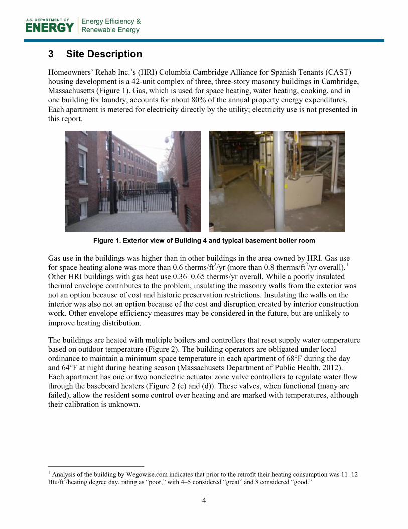
Homeowners’ Rehab Inc.’s (HRI) Columbia Cambridge Alliance for Spanish Tenants (CAST) housing development is a 42-unit complex of three, three-story masonry buildings in Cambridge, Massachusetts (Figure 1). Gas, which is used for space heating, water heating, cooking, and in one building for laundry, accounts for about 80% of the annual property energy expenditures. Each apartment is metered for electricity directly by the utility; electricity use is not presented in this report.
Figure 1. Exterior view of Building 4 and typical basement boiler room
Gas use in the buildings was higher than in other buildings in the area owned by HRI. Gas use for space heating alone was more than 0.6 therms/ft2/yr (more than 0.8 therms/ft2/yr overall).1 Other HRI buildings with gas heat use 0.36–0.65 therms/yr overall. While a poorly insulated thermal envelope contributes to the problem, insulating the masonry walls from the exterior was not an option because of cost and historic preservation restrictions. Insulating the walls on the interior was also not an option because of the cost and disruption created by interior construction work. Other envelope efficiency measures may be considered in the future, but are unlikely to improve heating distribution.
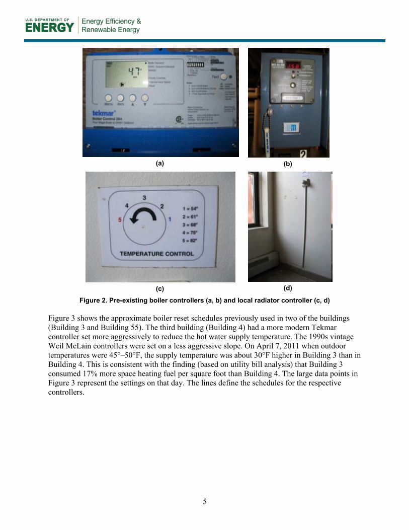
The buildings are heated with multiple boilers and controllers that reset supply water temperature based on outdoor temperature (Figure 2). The building operators are obligated under local ordinance to maintain a minimum space temperature in each apartment of 68°F during the day and 64°F at night during heating season (Massachusets Department of Public Health, 2012). Each apartment has one or two nonelectric actuator zone valve controllers to regulate water flow through the baseboard heaters (Figure 2 (c) and (d)). These valves, when functional (many are failed), allow the resident some control over heating and are marked with temperatures, although their calibration is unknown.
1 Analysis of the building by Wegowise.com indicates that prior to the retrofit their heating consumption was 11–12 Btu/ft2/heating degree day, rating as “poor,” with 4–5 considered “great” and 8 considered “good.”
5
(a)
(b)
(c)
(d)
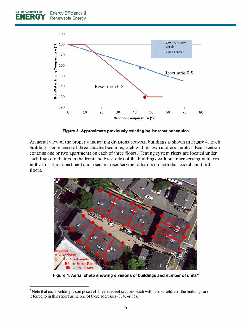
Figure 2. Pre-existing boiler controllers (a, b) and local radiator controller (c, d) Figure 3 shows the approximate boiler reset schedules previously used in two of the buildings (Building 3 and Building 55). The third building (Building 4) had a more modern Tekmar controller set more aggressively to reduce the hot water supply temperature. The 1990s vintage Weil McLain controllers were set on a less aggressive slope. On April 7, 2011 when outdoor temperatures were 45°–50°F, the supply temperature was about 30°F higher in Building 3 than in Building 4. This is consistent with the finding (based on utility bill analysis) that Building 3 consumed 17% more space heating fuel per square foot than Building 4. The large data points in Figure 3 represent the settings on that day. The lines define the schedules for the respective controllers.
6
Figure 3. Approximate previously existing boiler reset schedules
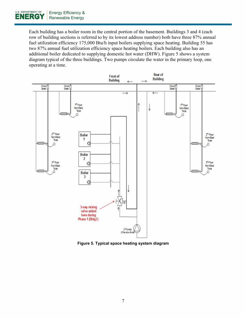
An aerial view of the property indicating divisions between buildings is shown in Figure 4. Each building is composed of three attached sections, each with its own address number. Each section contains one or two apartments on each of three floors. Heating system risers are located under each line of radiators in the front and back sides of the buildings with one riser serving radiators in the first-floor apartment and a second riser serving radiators on both the second and third floors.
Figure 4. Aerial photo showing divisions of buildings and number of units2
2 Note that each building is composed of three attached sections, each with its own address; the buildings are referred to in this report using one of these addresses (3, 4, or 55).
Reset ratio 0.5
Reset ratio 0.8
7
Each building has a boiler room in the central portion of the basement. Buildings 3 and 4 (each row of building sections is referred to by its lowest address number) both have three 87% annual fuel utilization efficiency 175,000 Btu/h input boilers supplying space heating. Building 55 has two 87% annual fuel utilization efficiency space heating boilers. Each building also has an additional boiler dedicated to supplying domestic hot water (DHW). Figure 5 shows a system diagram typical of the three buildings. Two pumps circulate the water in the primary loop, one operating at a time.
Figure 5. Typical space heating system diagram
8
4 Retrofit Strategies and Monitoring Plan
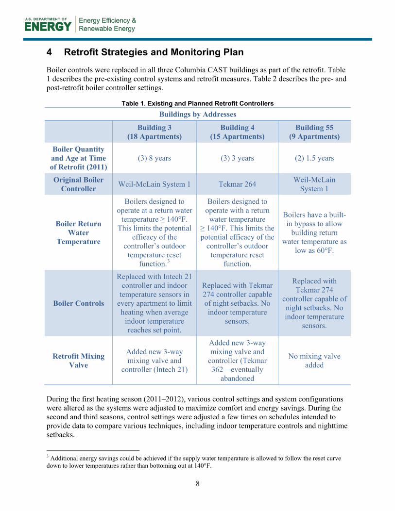
Boiler controls were replaced in all three Columbia CAST buildings as part of the retrofit. Table 1 describes the pre-existing control systems and retrofit measures. Table 2 describes the pre- and post-retrofit boiler controller settings.
Table 1. Existing and Planned Retrofit Controllers
During the first heating season (2011–2012), various control settings and system configurations were altered as the systems were adjusted to maximize comfort and energy savings. During the second and third seasons, control settings were adjusted a few times on schedules intended to provide data to compare various techniques, including indoor temperature controls and nighttime setbacks.
3 Additional energy savings could be achieved if the supply water temperature is allowed to follow the reset curve down to lower temperatures rather than bottoming out at 140°F.
Buildings by Addresses
Building 3 (18 Apartments)
Building 4 (15 Apartments)
Building 55 (9 Apartments)
Boiler Quantity and Age at Time of Retrofit (2011)
(3) 8 years (3) 3 years (2) 1.5 years
Original Boiler Controller Weil-McLain System 1 Tekmar 264 Weil-McLain
System 1
Boiler Return Water
Temperature
Boilers designed to operate at a return water
temperature ≥ 140°F. This limits the potential
efficacy of the controller’s outdoor
temperature reset function.3
Boilers designed to operate with a return
water temperature ≥ 140°F. This limits the potential efficacy of the
controller’s outdoor temperature reset
function.
Boilers have a built-in bypass to allow
building return water temperature as
low as 60°F.
Boiler Controls
Replaced with Intech 21 controller and indoor
temperature sensors in every apartment to limit heating when average
indoor temperature reaches set point.
Replaced with Tekmar 274 controller capable of night setbacks. No indoor temperature
sensors.
Replaced with Tekmar 274
controller capable of night setbacks. No indoor temperature
sensors.
Retrofit Mixing Valve
Added new 3-way mixing valve and
controller (Intech 21)
Added new 3-way mixing valve and
controller (Tekmar 362—eventually
abandoned
No mixing valve added
9
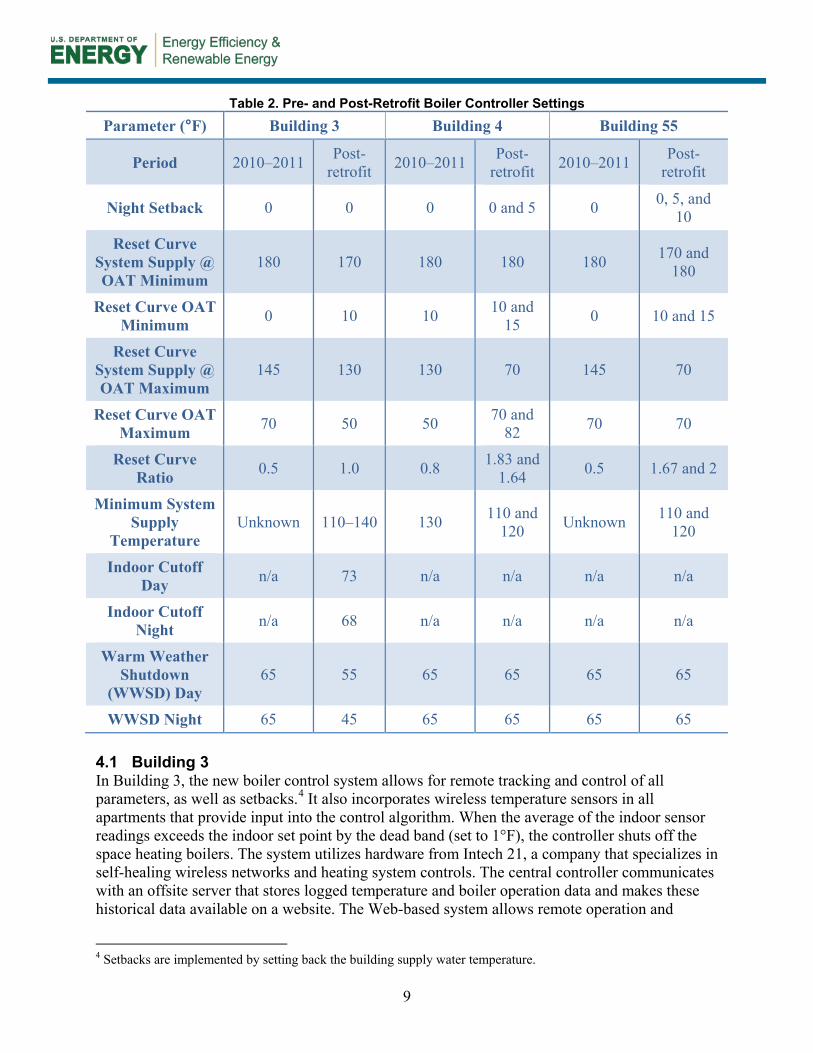
Table 2. Pre- and Post-Retrofit Boiler Controller Settings
4.1 Building 3 In Building 3, the new boiler control system allows for remote tracking and control of all parameters, as well as setbacks.4 It also incorporates wireless temperature sensors in all apartments that provide input into the control algorithm. When the average of the indoor sensor readings exceeds the indoor set point by the dead band (set to 1°F), the controller shuts off the space heating boilers. The system utilizes hardware from Intech 21, a company that specializes in self-healing wireless networks and heating system controls. The central controller communicates with an offsite server that stores logged temperature and boiler operation data and makes these historical data available on a website. The Web-based system allows remote operation and
4 Setbacks are implemented by setting back the building supply water temperature.
Parameter (°F) Building 3 Building 4 Building 55
Period 2010–2011 Post-retrofit 2010–2011 Post-
retrofit 2010–2011 Post-retrofit
Night Setback 0 0 0 0 and 5 0 0, 5, and 10
Reset Curve System Supply @ OAT Minimum
180 170 180 180 180 170 and 180
Reset Curve OAT Minimum 0 10 10 10 and
15 0 10 and 15
Reset Curve System Supply @ OAT Maximum
145 130 130 70 145 70
Reset Curve OAT Maximum 70 50 50 70 and
82 70 70
Reset Curve Ratio 0.5 1.0 0.8 1.83 and
1.64 0.5 1.67 and 2
Minimum System Supply
Temperature Unknown 110–140 130 110 and
120 Unknown 110 and 120
Indoor Cutoff Day n/a 73 n/a n/a n/a n/a
Indoor Cutoff Night n/a 68 n/a n/a n/a n/a
Warm Weather Shutdown
(WWSD) Day 65 55 65 65 65 65
WWSD Night 65 45 65 65 65 65
10
modification of the control parameters and provides real-time access to apartment temperature data so that building operators can ensure the legally required minimum heating temperature is provided to each apartment, without requiring an excessively large safety factor. One risk of this system is that tenants using supplemental heating (or cooling) could affect temperature sensor readings inadvertently or intentionally in an effort to obtain more (or less) heat. None of this behavior was observed, and the averaging of all apartment temperatures minimizes the impact any one apartment can have on the system.
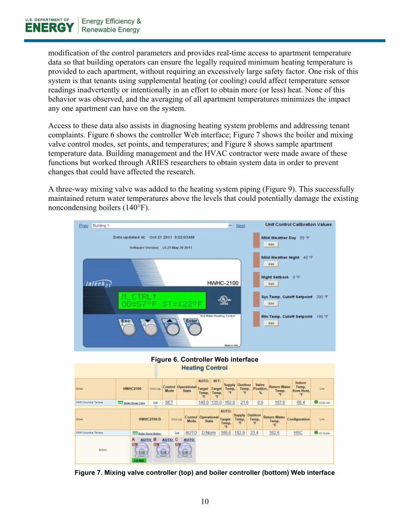
Access to these data also assists in diagnosing heating system problems and addressing tenant complaints. Figure 6 shows the controller Web interface; Figure 7 shows the boiler and mixing valve control modes, set points, and temperatures; and Figure 8 shows sample apartment temperature data. Building management and the HVAC contractor were made aware of these functions but worked through ARIES researchers to obtain system data in order to prevent changes that could have affected the research.
A three-way mixing valve was added to the heating system piping (Figure 9). This successfully maintained return water temperatures above the levels that could potentially damage the existing noncondensing boilers (140°F).
Figure 6. Controller Web interface
Figure 7. Mixing valve controller (top) and boiler controller (bottom) Web interface

11
Figure 8. Sample apartment temperature sensor data
Figure 9. Building 3 system configuration

12
4.2 Building 4 In Building 4, new boiler controls allow for setbacks and ORC as well as remote monitoring of all parameters. A three-way mixing valve was added (Figure 10) to maintain return water temperatures above the levels that could potentially damage the existing noncondensing boilers (140°F); however, as discussed in Appendix B this did not function as intended and was abandoned.
Figure 10. Building 4 system configuration
4.3 Building 55 The new controller in Building 55 is capable of setbacks. The boilers in Building 55 have a built-in bypass to mix hot water from the boiler outlet with colder return water (as low as 60°F) from the building prior to entry to the boiler sections when needed to prevent thermal shock and condensation of flue gases in the boilers’ heat exchangers. Therefore the addition of a new three-way mixing valve was unnecessary (Figure 11).

13
Figure 11. Building 55 system configuration
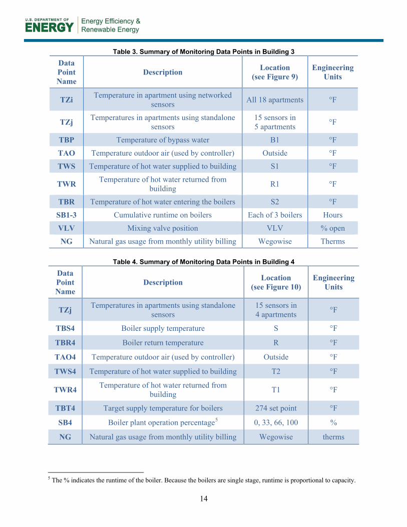
4.4 Data Collection Data to evaluate energy savings and comfort impacts were collected under various control scenarios for each building. Table 3, Table 4, and Table 5 summarize the data collection in Buildings 3, 4, and 55, respectively. Location codes in the tables refer to Figure 9, Figure 10, and Figure 11.
14
Table 3. Summary of Monitoring Data Points in Building 3
Table 4. Summary of Monitoring Data Points in Building 4
5 The % indicates the runtime of the boiler. Because the boilers are single stage, runtime is proportional to capacity.
Data Point Name
Description Location (see Figure 9)
Engineering Units
TZi Temperature in apartment using networked sensors All 18 apartments °F
TZj Temperatures in apartments using standalone sensors
15 sensors in 5 apartments °F
TBP Temperature of bypass water B1 °F
TAO Temperature outdoor air (used by controller) Outside °F
TWS Temperature of hot water supplied to building S1 °F
TWR Temperature of hot water returned from building R1 °F
TBR Temperature of hot water entering the boilers S2 °F
SB1-3 Cumulative runtime on boilers Each of 3 boilers Hours
VLV Mixing valve position VLV % open
NG Natural gas usage from monthly utility billing Wegowise Therms
Data Point Name
Description Location (see Figure 10)
Engineering Units
TZj Temperatures in apartments using standalone sensors
15 sensors in 4 apartments °F
TBS4 Boiler supply temperature S °F
TBR4 Boiler return temperature R °F
TAO4 Temperature outdoor air (used by controller) Outside °F
TWS4 Temperature of hot water supplied to building T2 °F
TWR4 Temperature of hot water returned from building T1 °F
TBT4 Target supply temperature for boilers 274 set point °F
SB4 Boiler plant operation percentage5 0, 33, 66, 100 %
NG Natural gas usage from monthly utility billing Wegowise therms
15
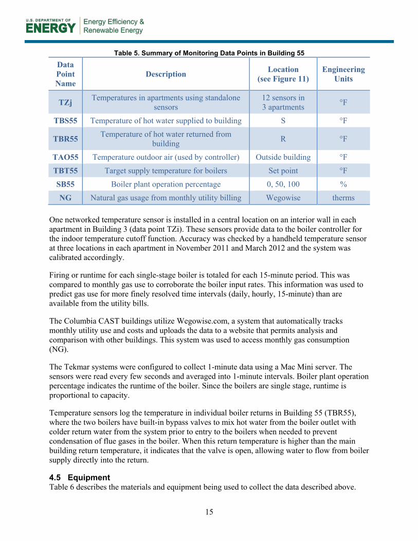
Table 5. Summary of Monitoring Data Points in Building 55
One networked temperature sensor is installed in a central location on an interior wall in each apartment in Building 3 (data point TZi). These sensors provide data to the boiler controller for the indoor temperature cutoff function. Accuracy was checked by a handheld temperature sensor at three locations in each apartment in November 2011 and March 2012 and the system was calibrated accordingly.
Firing or runtime for each single-stage boiler is totaled for each 15-minute period. This was compared to monthly gas use to corroborate the boiler input rates. This information was used to predict gas use for more finely resolved time intervals (daily, hourly, 15-minute) than are available from the utility bills.
The Columbia CAST buildings utilize Wegowise.com, a system that automatically tracks monthly utility use and costs and uploads the data to a website that permits analysis and comparison with other buildings. This system was used to access monthly gas consumption (NG).
The Tekmar systems were configured to collect 1-minute data using a Mac Mini server. The sensors were read every few seconds and averaged into 1-minute intervals. Boiler plant operation percentage indicates the runtime of the boiler. Since the boilers are single stage, runtime is proportional to capacity.
Temperature sensors log the temperature in individual boiler returns in Building 55 (TBR55), where the two boilers have built-in bypass valves to mix hot water from the boiler outlet with colder return water from the system prior to entry to the boilers when needed to prevent condensation of flue gases in the boiler. When this return temperature is higher than the main building return temperature, it indicates that the valve is open, allowing water to flow from boiler supply directly into the return.
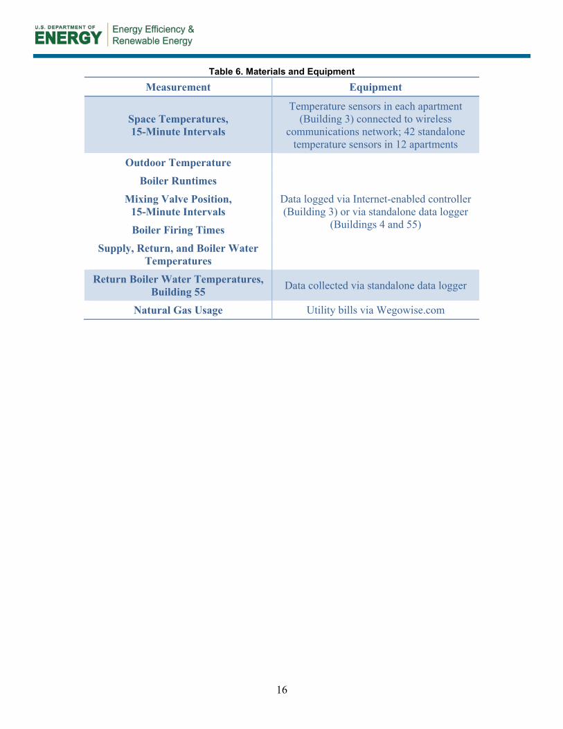
4.5 Equipment Table 6 describes the materials and equipment being used to collect the data described above.
Data Point Name
Description Location (see Figure 11)
Engineering Units
TZj Temperatures in apartments using standalone sensors
12 sensors in 3 apartments °F
TBS55 Temperature of hot water supplied to building S °F
TBR55 Temperature of hot water returned from building R °F
TAO55 Temperature outdoor air (used by controller) Outside building °F
TBT55 Target supply temperature for boilers Set point °F
SB55 Boiler plant operation percentage 0, 50, 100 %
NG Natural gas usage from monthly utility billing Wegowise therms
16
Table 6. Materials and Equipment
Measurement Equipment
Space Temperatures, 15-Minute Intervals
Temperature sensors in each apartment (Building 3) connected to wireless
communications network; 42 standalone temperature sensors in 12 apartments
Outdoor Temperature
Data logged via Internet-enabled controller (Building 3) or via standalone data logger
(Buildings 4 and 55)
Boiler Runtimes Mixing Valve Position,
15-Minute Intervals Boiler Firing Times
Supply, Return, and Boiler Water Temperatures
Return Boiler Water Temperatures, Building 55 Data collected via standalone data logger
Natural Gas Usage Utility bills via Wegowise.com
17
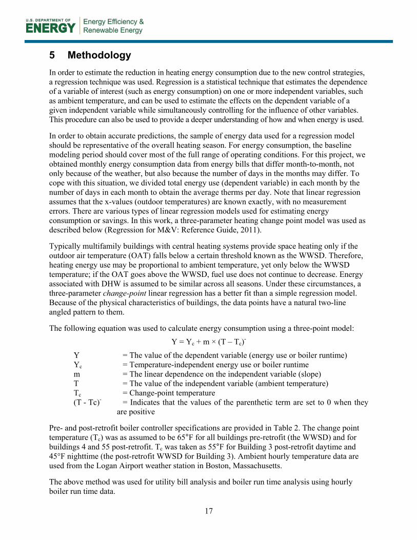
5 Methodology In order to estimate the reduction in heating energy consumption due to the new control strategies, a regression technique was used. Regression is a statistical technique that estimates the dependence of a variable of interest (such as energy consumption) on one or more independent variables, such as ambient temperature, and can be used to estimate the effects on the dependent variable of a given independent variable while simultaneously controlling for the influence of other variables. This procedure can also be used to provide a deeper understanding of how and when energy is used.
In order to obtain accurate predictions, the sample of energy data used for a regression model should be representative of the overall heating season. For energy consumption, the baseline modeling period should cover most of the full range of operating conditions. For this project, we obtained monthly energy consumption data from energy bills that differ month-to-month, not only because of the weather, but also because the number of days in the months may differ. To cope with this situation, we divided total energy use (dependent variable) in each month by the number of days in each month to obtain the average therms per day. Note that linear regression assumes that the x-values (outdoor temperatures) are known exactly, with no measurement errors. There are various types of linear regression models used for estimating energy consumption or savings. In this work, a three-parameter heating change point model was used as described below (Regression for M&V: Reference Guide, 2011).
Typically multifamily buildings with central heating systems provide space heating only if the outdoor air temperature (OAT) falls below a certain threshold known as the WWSD. Therefore, heating energy use may be proportional to ambient temperature, yet only below the WWSD temperature; if the OAT goes above the WWSD, fuel use does not continue to decrease. Energy associated with DHW is assumed to be similar across all seasons. Under these circumstances, a three-parameter change-point linear regression has a better fit than a simple regression model. Because of the physical characteristics of buildings, the data points have a natural two-line angled pattern to them.
The following equation was used to calculate energy consumption using a three-point model:
Y = Yc + m × (T – Tc)-
Y = The value of the dependent variable (energy use or boiler runtime) Yc = Temperature-independent energy use or boiler runtime m = The linear dependence on the independent variable (slope) T = The value of the independent variable (ambient temperature) Tc = Change-point temperature (T - Tc)- = Indicates that the values of the parenthetic term are set to 0 when they
are positive
Pre- and post-retrofit boiler controller specifications are provided in Table 2. The change point temperature (Tc) was as assumed to be 65°F for all buildings pre-retrofit (the WWSD) and for buildings 4 and 55 post-retrofit. Tc was taken as 55°F for Building 3 post-retrofit daytime and 45°F nighttime (the post-retrofit WWSD for Building 3). Ambient hourly temperature data are used from the Logan Airport weather station in Boston, Massachusetts.
The above method was used for utility bill analysis and boiler run time analysis using hourly boiler run time data.
18
6 Results and Analysis
Each building was operated in multiple control states during the monitoring period. This section describes the control strategies employed, their effect on system operation, and their impact on boiler runtime and utility bills.
6.1 Building 3 The new control strategy for Building 3 incorporated two major changes from the previously existing controller.
1. Reset schedule: The original controller was set for supply temperature of 180°F at 0°F outdoor temperature, decreasing linearly to 145°F at 70°F outdoor temperature (reset ratio of 0.5) with a WWSD of 65°F for both day and night. The new controller was set for daytime to a return temperature of 170°F at 10°F outdoors, and decreasing linearly to 130°F at 50°F outdoors (reset ratio of 1.0) with a WWSD of 55°F. For nighttime, the return water temp and WWSD were 10°F lower (Figure 12). Controlling to return instead of supply water temperature is thought to result in a more stable system.
Figure 12. Building 3 controller reset schedules
2. Indoor cutoff: The new controller can shut off the boilers when the average indoor
temperature from apartment temperature sensors is above a desired set point (established as 73°F daytime and 68°F nighttime). This function was enabled and disabled a few times to collect data in both modes to observe the effect on boiler run time. Table 7 shows data collection period for various control settings.
19
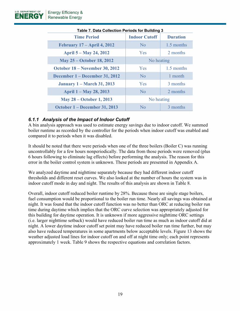
Table 7. Data Collection Periods for Building 3
6.1.1 Analysis of the Impact of Indoor Cutoff A bin analysis approach was used to estimate energy savings due to indoor cutoff. We summed boiler runtime as recorded by the controller for the periods when indoor cutoff was enabled and compared it to periods when it was disabled.
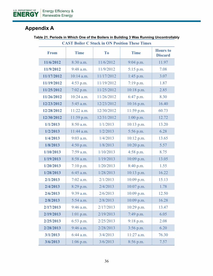
It should be noted that there were periods when one of the three boilers (Boiler C) was running uncontrollably for a few hours nonperiodically. The data from those periods were removed (plus 6 hours following to eliminate lag effects) before performing the analysis. The reason for this error in the boiler control system is unknown. These periods are presented in Appendix A.
We analyzed daytime and nighttime separately because they had different indoor cutoff thresholds and different reset curves. We also looked at the number of hours the system was in indoor cutoff mode in day and night. The results of this analysis are shown in Table 8.
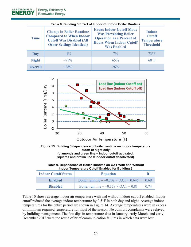
Overall, indoor cutoff reduced boiler runtime by 28%. Because these are single stage boilers, fuel consumption would be proportional to the boiler run time. Nearly all savings was obtained at night. It was found that the indoor cutoff function was no better than ORC at reducing boiler run time during daytime which implies that the ORC curve selection was appropriately adjusted for this building for daytime operation. It is unknown if more aggressive nighttime ORC settings (i.e. larger nighttime setback) would have reduced boiler run time as much as indoor cutoff did at night. A lower daytime indoor cutoff set point may have reduced boiler run time further, but may also have reduced temperatures in some apartments below acceptable levels. Figure 13 shows the weather adjusted load lines for indoor cutoff on and off at night time only; each point represents approximately 1 week. Table 9 shows the respective equations and correlation factors.
Time Period Indoor Cutoff Duration
February 17 – April 4, 2012 No 1.5 months
April 5 – May 24, 2012 Yes 2 months
May 25 – October 18, 2012 No heating
October 18 – November 30, 2012 Yes 1.5 months
December 1 – December 31, 2012 No 1 month
January 1 – March 31, 2013 Yes 3 months
April 1 – May 28, 2013 No 2 months
May 28 – October 1, 2013 No heating
October 1 – December 31, 2013 No 3 months
20
Table 8. Building 3 Effect of Indoor Cutoff on Boiler Runtime
Figure 13. Building 3 dependence of boiler runtime on indoor temperature
cutoff at night only (diamonds and green line = indoor cutoff activated; squares and brown line = indoor cutoff deactivated)
Table 9. Dependence of Boiler Runtime on OAT With and Without
Indoor Temperature Cutoff Enabled for Building 3
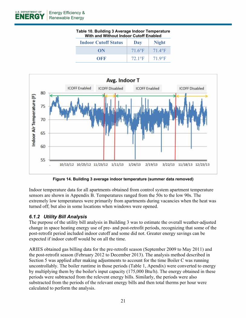
Table 10 shows average indoor air temperature with and without indoor cut off enabled. Indoor cutoff reduced the average indoor temperature by 0.5°F in both day and night. Average indoor temperatures for the entire period are shown in Figure 14. Average temperatures were in excess of minimum required temperature for most of the season. No comfort complaints were relayed by building management. The few dips in temperature data in January, early March, and early December 2013 were the result of brief communication failures in which data were lost.
Time
Change in Boiler Runtime Compared to When Indoor Cutoff Was Disabled (All Other Settings Identical)
Hours Indoor Cutoff Mode Was Preventing Boiler
Operation as a Percent of Hours When Indoor Cutoff
Was Enabled
Indoor Cutoff
Temperature Threshold
Day –1% 7% 73°F
Night –71% 65% 68°F
Overall –28% 26%
Indoor Cutoff Status Equation R2
Enabled Boiler runtime = –0.202 × OAT + 0.645 0.69
Disabled Boiler runtime = –0.329 × OAT + 0.81 0.74
Load line (Indoor Cutoff on) Load line (Indoor Cutoff off)
21
Table 10. Building 3 Average Indoor Temperature With and Without Indoor Cutoff Enabled
Figure 14. Building 3 average indoor temperature (summer data removed)
Indoor temperature data for all apartments obtained from control system apartment temperature sensors are shown in Appendix B. Temperatures ranged from the 50s to the low 90s. The extremely low temperatures were primarily from apartments during vacancies when the heat was turned off; but also in some locations when windows were opened.
6.1.2 Utility Bill Analysis The purpose of the utility bill analysis in Building 3 was to estimate the overall weather-adjusted change in space heating energy use of pre- and post-retrofit periods, recognizing that some of the post-retrofit period included indoor cutoff and some did not. Greater energy savings can be expected if indoor cutoff would be on all the time.
ARIES obtained gas billing data for the pre-retrofit season (September 2009 to May 2011) and the post-retrofit season (February 2012 to December 2013). The analysis method described in Section 5 was applied after making adjustments to account for the time Boiler C was running uncontrollably. The boiler runtime in those periods (Table 1, Apendix) were converted to energy by multiplying them by the boiler's input capacity (175,000 Btu/h). The energy obtained in these periods were subtracted from the relevent energy bills. Similarly, the periods were also substracted from the periods of the relevant energy bills and then total therms per hour were calculated to perform the analysis.
Indoor Cutoff Status Day Night
ON 71.6°F 71.4°F
OFF 72.1°F 71.9°F

22
Figure 15 shows the dependence of space heating energy consumption in the building on outdoor air temperature for pre- and post-retrofit periods. Table 11 shows the equations of the load lines and values of coefficients of determination for pre- and post-retrofits periods. Total predicted savings from the retrofit for Building 3 are presented in Table 12.
Table 11. Building 3 Dependence of Energy Consumption on OAT (Slope) and Coefficient of Determination (R2) for Building 3
Figure 15. Building 3 dependence of energy consumption on OAT
(diamonds and green line = post-retrofit; squares and brown line = pre-retrofit)
Period Equation R2
Pre-Retrofit (2010–2011) Gas use = –1.381 × OAT + 10.349 0.972
Post-Retrofit (2011–2012) Gas use = –1.522 × OAT + 10.660 0.951
23
Table 12. Building 3 Pre- and Post-Retrofit Heating and Total Energy Consumption and Reduction (therms) for Building 3
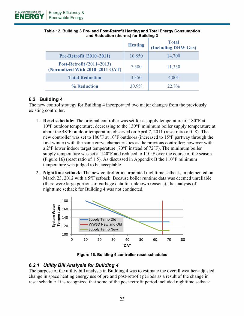
6.2 Building 4 The new control strategy for Building 4 incorporated two major changes from the previously existing controller.
1. Reset schedule: The original controller was set for a supply temperature of 180°F at 10°F outdoor temperature, decreasing to the 130°F minimum boiler supply temperature at about the 48°F outdoor temperature observed on April 7, 2011 (reset ratio of 0.8). The new controller was set to 180°F at 10°F outdoors (increased to 15°F partway through the first winter) with the same curve characteristics as the previous controller; however with a 2°F lower indoor target temperature (70°F instead of 72°F). The minimum boiler supply temperature was set at 140°F and reduced to 110°F over the course of the season (Figure 16) (reset ratio of 1.5). As discussed in Appendix B the 110°F minimum temperature was judged to be acceptable.
2. Nighttime setback: The new controller incorporated nighttime setback, implemented on March 23, 2012 with a 5°F setback. Because boiler runtime data was deemed unreliable (there were large portions of garbage data for unknown reasons), the analysis of nighttime setback for Building 4 was not conducted.
Figure 16. Building 4 controller reset schedules
6.2.1 Utility Bill Analysis for Building 4 The purpose of the utility bill analysis in Building 4 was to estimate the overall weather-adjusted change in space heating energy use of pre and post-retrofit periods as a result of the change in reset schedule. It is recognized that some of the post-retrofit period included nighttime setback
100
120
140
160
180
0 10 20 30 40 50 60 70 80
Syst
em W
ater
Te
mpe
ratu
re
OAT
Supply Temp OldWWSD New and OldSupply Temp New
Heating Total (Including DHW Gas)
Pre-Retrofit (2010–2011) 10,850 14,700
Post-Retrofit (2011–2013) (Normalized With 2010–2011 OAT) 7,500 11,350
Total Reduction 3,350 4,001
% Reduction 30.9% 22.8%
24
and some did not; however, nighttime setback had little effect in Building 55, as will be described below.
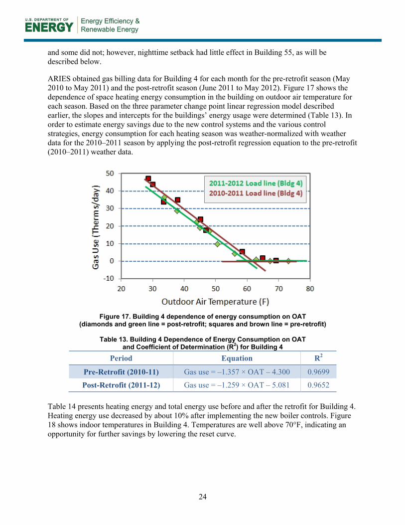
ARIES obtained gas billing data for Building 4 for each month for the pre-retrofit season (May 2010 to May 2011) and the post-retrofit season (June 2011 to May 2012). Figure 17 shows the dependence of space heating energy consumption in the building on outdoor air temperature for each season. Based on the three parameter change point linear regression model described earlier, the slopes and intercepts for the buildings’ energy usage were determined (Table 13). In order to estimate energy savings due to the new control systems and the various control strategies, energy consumption for each heating season was weather-normalized with weather data for the 2010–2011 season by applying the post-retrofit regression equation to the pre-retrofit (2010–2011) weather data.
Figure 17. Building 4 dependence of energy consumption on OAT
(diamonds and green line = post-retrofit; squares and brown line = pre-retrofit)
Table 13. Building 4 Dependence of Energy Consumption on OAT and Coefficient of Determination (R2) for Building 4
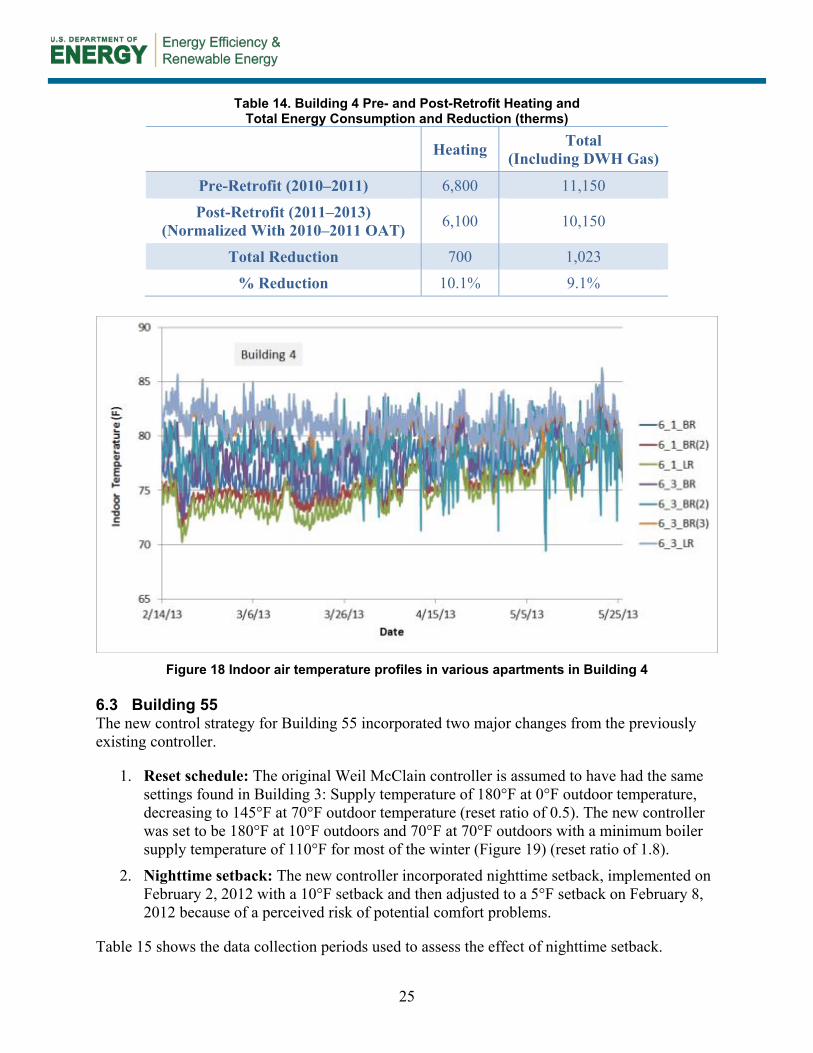
Table 14 presents heating energy and total energy use before and after the retrofit for Building 4. Heating energy use decreased by about 10% after implementing the new boiler controls. Figure 18 shows indoor temperatures in Building 4. Temperatures are well above 70°F, indicating an opportunity for further savings by lowering the reset curve.
Period Equation R2
Pre-Retrofit (2010-11) Gas use = –1.357 × OAT – 4.300 0.9699
Post-Retrofit (2011-12) Gas use = –1.259 × OAT – 5.081 0.9652
25
Table 14. Building 4 Pre- and Post-Retrofit Heating and Total Energy Consumption and Reduction (therms)
Figure 18 Indoor air temperature profiles in various apartments in Building 4
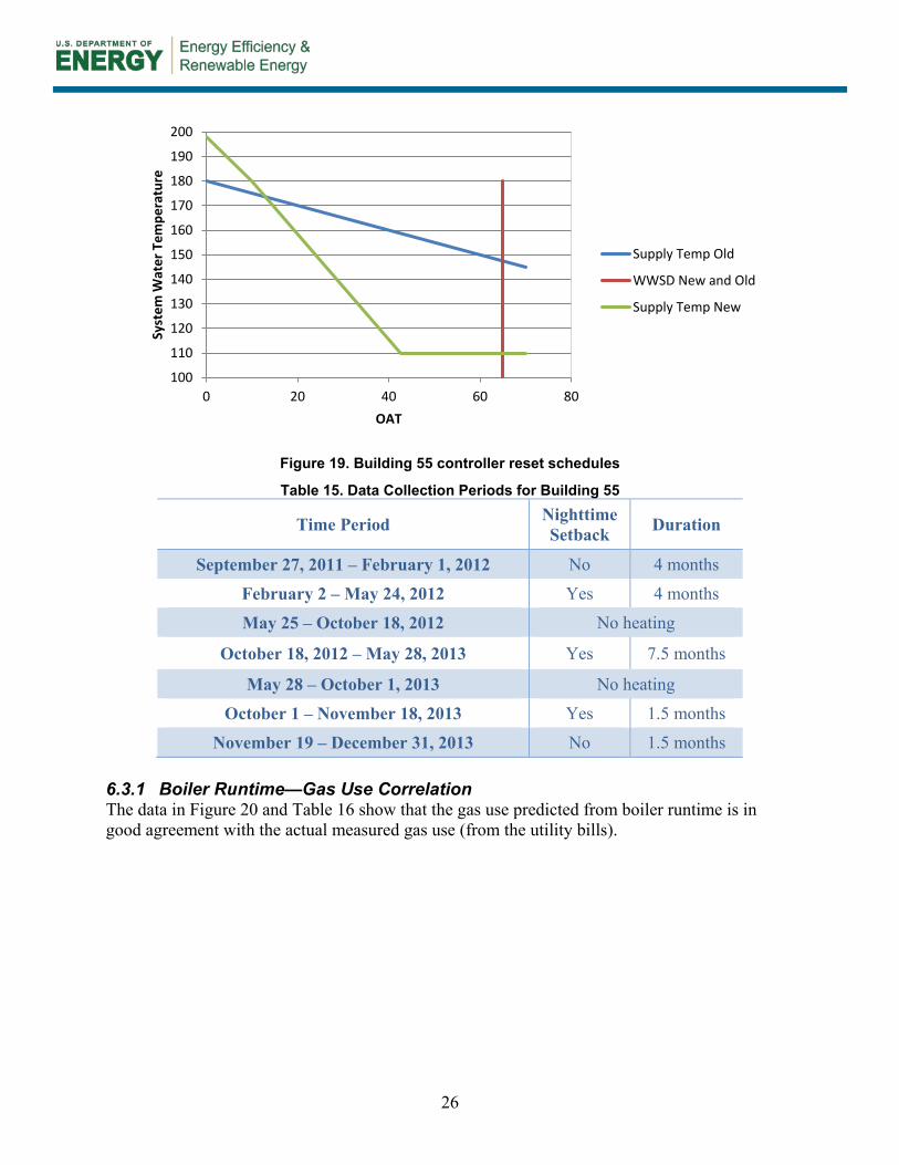
6.3 Building 55 The new control strategy for Building 55 incorporated two major changes from the previously existing controller.
1. Reset schedule: The original Weil McClain controller is assumed to have had the same settings found in Building 3: Supply temperature of 180°F at 0°F outdoor temperature, decreasing to 145°F at 70°F outdoor temperature (reset ratio of 0.5). The new controller was set to be 180°F at 10°F outdoors and 70°F at 70°F outdoors with a minimum boiler supply temperature of 110°F for most of the winter (Figure 19) (reset ratio of 1.8).
2. Nighttime setback: The new controller incorporated nighttime setback, implemented on February 2, 2012 with a 10°F setback and then adjusted to a 5°F setback on February 8, 2012 because of a perceived risk of potential comfort problems.
Table 15 shows the data collection periods used to assess the effect of nighttime setback.
Heating Total (Including DWH Gas)
Pre-Retrofit (2010–2011) 6,800 11,150
Post-Retrofit (2011–2013) (Normalized With 2010–2011 OAT) 6,100 10,150
Total Reduction 700 1,023
% Reduction 10.1% 9.1%
26
Figure 19. Building 55 controller reset schedules
Table 15. Data Collection Periods for Building 55
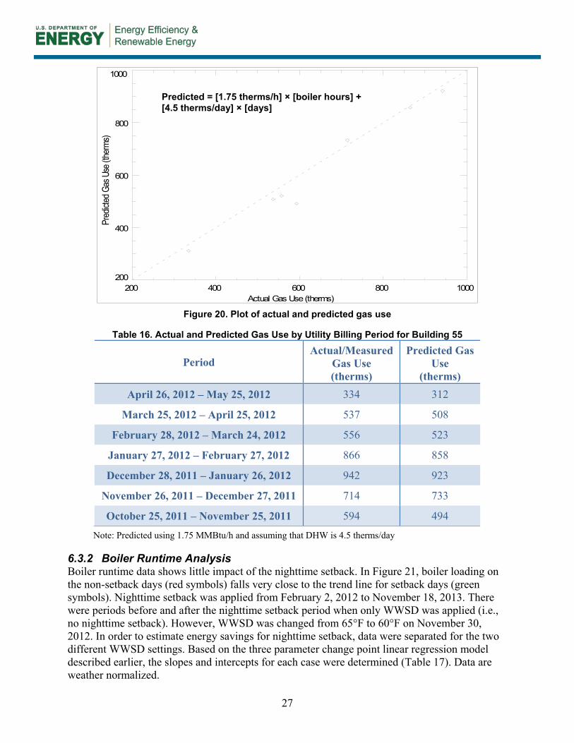
6.3.1 Boiler Runtime—Gas Use Correlation The data in Figure 20 and Table 16 show that the gas use predicted from boiler runtime is in good agreement with the actual measured gas use (from the utility bills).
100
110
120
130
140
150
160
170
180
190
200
0 20 40 60 80
Syst
em W
ater
Tem
pera
ture
OAT
Supply Temp Old
WWSD New and Old
Supply Temp New
Time Period Nighttime Setback Duration
September 27, 2011 – February 1, 2012 No 4 months
February 2 – May 24, 2012 Yes 4 months
May 25 – October 18, 2012 No heating
October 18, 2012 – May 28, 2013 Yes 7.5 months
May 28 – October 1, 2013 No heating
October 1 – November 18, 2013 Yes 1.5 months
November 19 – December 31, 2013 No 1.5 months
27
Figure 20. Plot of actual and predicted gas use
Table 16. Actual and Predicted Gas Use by Utility Billing Period for Building 55
Note: Predicted using 1.75 MMBtu/h and assuming that DHW is 4.5 therms/day
6.3.2 Boiler Runtime Analysis Boiler runtime data shows little impact of the nighttime setback. In Figure 21, boiler loading on the non-setback days (red symbols) falls very close to the trend line for setback days (green symbols). Nighttime setback was applied from February 2, 2012 to November 18, 2013. There were periods before and after the nighttime setback period when only WWSD was applied (i.e., no nighttime setback). However, WWSD was changed from 65°F to 60°F on November 30, 2012. In order to estimate energy savings for nighttime setback, data were separated for the two different WWSD settings. Based on the three parameter change point linear regression model described earlier, the slopes and intercepts for each case were determined (Table 17). Data are weather normalized.
200 400 600 800 1000Actual Gas Use (therms)
200
400
600
800
1000
Pred
icted
Gas
Use
(the
rms)
Period Actual/Measured
Gas Use (therms)
Predicted Gas Use
(therms) April 26, 2012 – May 25, 2012 334 312
March 25, 2012 – April 25, 2012 537 508
February 28, 2012 – March 24, 2012 556 523
January 27, 2012 – February 27, 2012 866 858
December 28, 2011 – January 26, 2012 942 923
November 26, 2011 – December 27, 2011 714 733
October 25, 2011 – November 25, 2011 594 494
Predicted = [1.75 therms/h] × [boiler hours] + [4.5 therms/day] × [days]
28
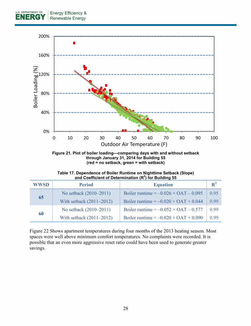
Figure 21. Plot of boiler loading—comparing days with and without setback
through January 31, 2014 for Building 55 (red = no setback, green = with setback)
Table 17. Dependence of Boiler Runtime on Nighttime Setback (Slope)
and Coefficient of Determination (R2) for Building 55
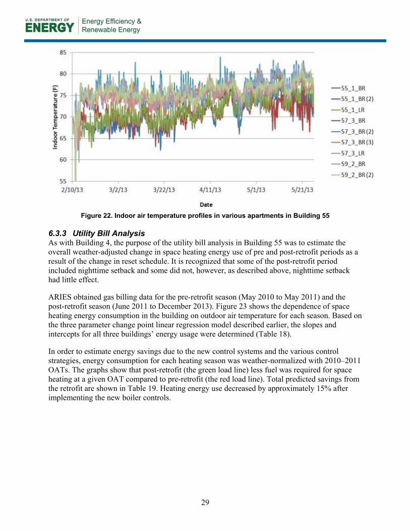
Figure 22 Shows apartment temperatures during four months of the 2013 heating season. Most spaces were well above minimum comfort temperatures. No complaints were recorded. It is possible that an even more aggressive reset ratio could have been used to generate greater savings.
0%
40%
80%
120%
160%
200%
0 10 20 30 40 50 60 70 80 90 100
Boile
r Loa
ding
(%)
Outdoor Air Temperature (F)
WWSD Period Equation R2
65 No setback (2010–2011) Boiler runtime = –0.026 × OAT – 0.095 0.95
With setback (2011–2012) Boiler runtime = –0.020 × OAT + 0.044 0.99
60 No setback (2010–2011) Boiler runtime = –0.052 × OAT – 0.577 0.99
With setback (2011–2012) Boiler runtime = –0.020 × OAT + 0.090 0.99
29
Figure 22. Indoor air temperature profiles in various apartments in Building 55
6.3.3 Utility Bill Analysis As with Building 4, the purpose of the utility bill analysis in Building 55 was to estimate the overall weather-adjusted change in space heating energy use of pre and post-retrofit periods as a result of the change in reset schedule. It is recognized that some of the post-retrofit period included nighttime setback and some did not, however, as described above, nighttime setback had little effect.
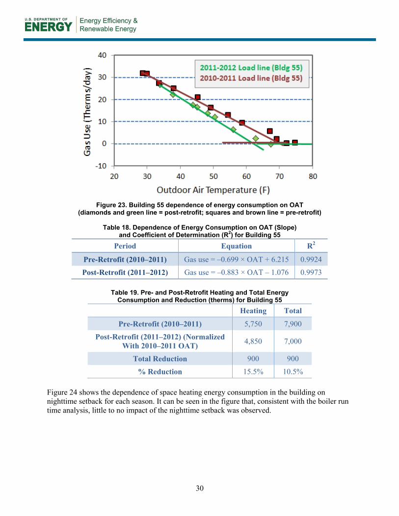
ARIES obtained gas billing data for the pre-retrofit season (May 2010 to May 2011) and the post-retrofit season (June 2011 to December 2013). Figure 23 shows the dependence of space heating energy consumption in the building on outdoor air temperature for each season. Based on the three parameter change point linear regression model described earlier, the slopes and intercepts for all three buildings’ energy usage were determined (Table 18).
In order to estimate energy savings due to the new control systems and the various control strategies, energy consumption for each heating season was weather-normalized with 2010–2011 OATs. The graphs show that post-retrofit (the green load line) less fuel was required for space heating at a given OAT compared to pre-retrofit (the red load line). Total predicted savings from the retrofit are shown in Table 19. Heating energy use decreased by approximately 15% after implementing the new boiler controls.
30
Figure 23. Building 55 dependence of energy consumption on OAT
(diamonds and green line = post-retrofit; squares and brown line = pre-retrofit)
Table 18. Dependence of Energy Consumption on OAT (Slope) and Coefficient of Determination (R2) for Building 55
Table 19. Pre- and Post-Retrofit Heating and Total Energy Consumption and Reduction (therms) for Building 55
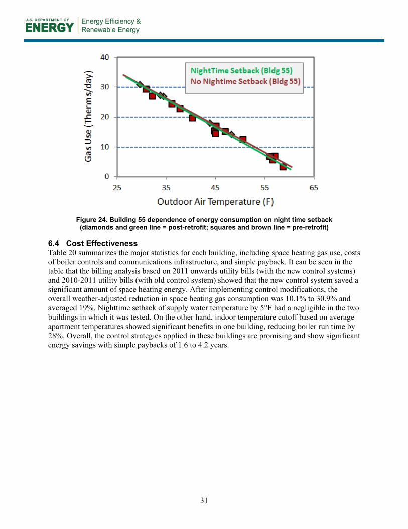
Figure 24 shows the dependence of space heating energy consumption in the building on nighttime setback for each season. It can be seen in the figure that, consistent with the boiler run time analysis, little to no impact of the nighttime setback was observed.
Period Equation R2
Pre-Retrofit (2010–2011) Gas use = –0.699 × OAT + 6.215 0.9924
Post-Retrofit (2011–2012) Gas use = –0.883 × OAT – 1.076 0.9973
Heating Total
Pre-Retrofit (2010–2011) 5,750 7,900
Post-Retrofit (2011–2012) (Normalized With 2010–2011 OAT) 4,850 7,000
Total Reduction 900 900
% Reduction 15.5% 10.5%
31
Figure 24. Building 55 dependence of energy consumption on night time setback
(diamonds and green line = post-retrofit; squares and brown line = pre-retrofit)
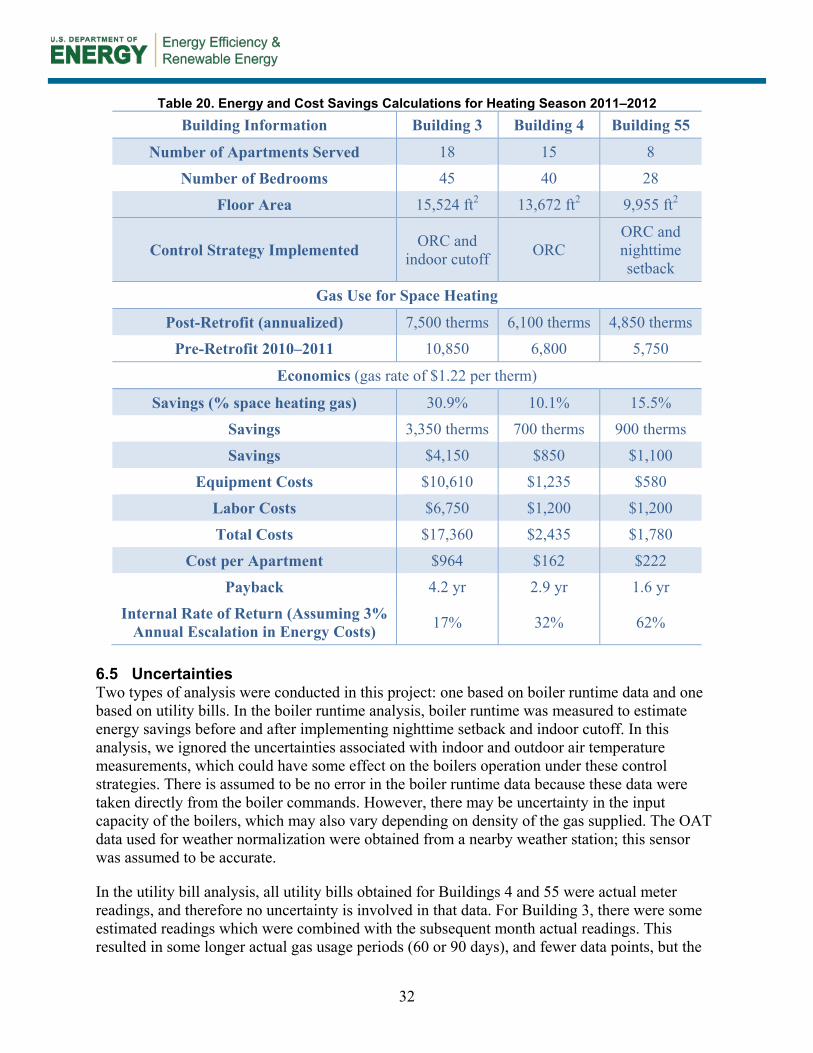
6.4 Cost Effectiveness Table 20 summarizes the major statistics for each building, including space heating gas use, costs of boiler controls and communications infrastructure, and simple payback. It can be seen in the table that the billing analysis based on 2011 onwards utility bills (with the new control systems) and 2010-2011 utility bills (with old control system) showed that the new control system saved a significant amount of space heating energy. After implementing control modifications, the overall weather-adjusted reduction in space heating gas consumption was 10.1% to 30.9% and averaged 19%. Nighttime setback of supply water temperature by 5°F had a negligible in the two buildings in which it was tested. On the other hand, indoor temperature cutoff based on average apartment temperatures showed significant benefits in one building, reducing boiler run time by 28%. Overall, the control strategies applied in these buildings are promising and show significant energy savings with simple paybacks of 1.6 to 4.2 years.
32
Table 20. Energy and Cost Savings Calculations for Heating Season 2011–2012
6.5 Uncertainties Two types of analysis were conducted in this project: one based on boiler runtime data and one based on utility bills. In the boiler runtime analysis, boiler runtime was measured to estimate energy savings before and after implementing nighttime setback and indoor cutoff. In this analysis, we ignored the uncertainties associated with indoor and outdoor air temperature measurements, which could have some effect on the boilers operation under these control strategies. There is assumed to be no error in the boiler runtime data because these data were taken directly from the boiler commands. However, there may be uncertainty in the input capacity of the boilers, which may also vary depending on density of the gas supplied. The OAT data used for weather normalization were obtained from a nearby weather station; this sensor was assumed to be accurate.
In the utility bill analysis, all utility bills obtained for Buildings 4 and 55 were actual meter readings, and therefore no uncertainty is involved in that data. For Building 3, there were some estimated readings which were combined with the subsequent month actual readings. This resulted in some longer actual gas usage periods (60 or 90 days), and fewer data points, but the
Building Information Building 3 Building 4 Building 55
Number of Apartments Served 18 15 8
Number of Bedrooms 45 40 28
Floor Area 15,524 ft2 13,672 ft2 9,955 ft2
Control Strategy Implemented ORC and indoor cutoff ORC
ORC and nighttime setback
Gas Use for Space Heating
Post-Retrofit (annualized) 7,500 therms 6,100 therms 4,850 therms
Pre-Retrofit 2010–2011 10,850 6,800 5,750
Economics (gas rate of $1.22 per therm)
Savings (% space heating gas) 30.9% 10.1% 15.5%
Savings 3,350 therms 700 therms 900 therms
Savings $4,150 $850 $1,100
Equipment Costs $10,610 $1,235 $580
Labor Costs $6,750 $1,200 $1,200
Total Costs $17,360 $2,435 $1,780
Cost per Apartment $964 $162 $222
Payback 4.2 yr 2.9 yr 1.6 yr
Internal Rate of Return (Assuming 3% Annual Escalation in Energy Costs) 17% 32% 62%
33
correlation coefficient remained acceptable. Gas utility bills also include uncertainty as to gas usage for space heating relative to water heating or cooking in addition to using the average monthly total to estimate daily gas use.
6.6 Other Impacts The retrofit control systems are expected to provide other nonenergy benefits to building residents and management, including:
• Occupant comfort: The heating control system is intended to improve comfort by ensuring adequate heat and reducing overheating of apartments. Achieving optimum savings may result in some apartments being cooler than occupants have become accustomed to, but still within the legal limits (Gifford 2004). A survey was conducted to gauge occupant satisfaction with the heating system, and repeated in 2012–2013. Very few responses were received (a total of fewer than 10 for both surveys combined). One way of interpreting the lack of response is to assume that residents had few complaints about the heat (very few complaints were made to management as well). The indoor temperature data also bear this out; most apartments remained warmer than 70°F throughout the winter. Because no indoor temperature data are available from prior to the retrofit, it is unknown if temperatures were reduced as a result of the new controllers.
• Occupant health and safety: Reducing overheating reduces drying of indoor air and limits the need to open windows to allow excess heat to escape in winter.
• Code compliance: The system employed in Building 3 enables the property manager to more precisely and reliably comply with minimum/maximum heat laws for rental apartments through online monitoring and logging of individual apartment temperatures.
• Building and equipment maintainability: Web-enabled visibility of apartment temperatures (Building 3) and boiler/valve status permits maintenance personnel to more rapidly detect and react to maintenance issues and complaints.

34
7 Conclusions
This report summarizes the results of a boiler controls retrofit in three buildings in Cambridge, Massachusetts. Controllers in all three buildings were replaced and the data collected for two heating seasons. The following research questions were addressed:
Question 1: What are the energy and comfort impacts of retrofitting multifamily central boiler controllers using ORC?
Answer: A billing analysis comparing 2011 onward utility bills (with new control system) and 2010–2011 utility bills (with old control systems) showed that the new control systems saved a significant amount of space heating energy. The overall weather-adjusted reduction in space heating gas consumption was 10%–15% from improvements to ORC. The simple average payback is projected to be less than 3 years. Indoor air temperature data obtained from temperature sensors mounted in various apartments in each building indicate that the temperature was generally within the comfort range throughout the buildings for the entire winter. These results lead to the conclusion that boiler control improvements in hydronically heated buildings can be a cost-effective and simple-to-implement strategy with large potential energy savings.
Question 2: How does a control system incorporating apartment temperature data compare in cost and performance with well-tuned ORC strategies?
Answer: An indoor temperature cutoff control feature based on average apartment temperatures showed significant benefits in the one building where it was tested. Indoor cutoff control reduced boiler runtime by 28%. Nearly all these savings were obtained in the night, which had lower indoor temperature cutoff (68°F) compared to the day (73°F). This implies that the ORC curve selection was appropriately adjusted for this building for daytime operation and that ORC alone can potentially achieve similar results if properly tuned to the building.
Question 3: What is the impact on space heating energy consumption of nighttime setback of supply water temperature on multifamily buildings with central hydronic space heating?
Answer: The data show negligible effect of a 5°F nighttime setback of supply water temperature in the one building in which results were obtained. It may be that 5°F was too small a setback and that the building mass dampened the effect of the setback.
35
References
Center for Energy and the Environment. (2006). Outdoor Reset and Cutout Control. Center for Energy and Environment: www.mncee.org/pdf/multifamily/outdrreset_coutoutcon.pdf.
CNT Energy. (2010). Boiler Controls and Sensors. Retrieved April 2011, from Energy Savers « CNT Energy: www.cntenergy.org/media/Boiler-Controls-Sensors.pdf.
Gifford, H. (2004). Choosing Thermostatic Radiator Valves. American Boiler Manufacturer’s Association.
Hewett, M.J.; Peterson, G.A. (1984). “Measured Energy Savings From Outdoor Resets in Modern, Hydronically Heated Apartment Buildings.” Proceedings of the American Council for an Energy Efficient Economy 1984 Summer Study C:135–152. Washington. D.C.: ACEEE.
Liao, Z.; Dexter, A. (2004). “The Potential for Energy Saving in Heating Systems Through Improving Boiler Controls.” Energy and Buildings 261–271.
Liao, Z.; Dexter, A. (2005). “An Experimental Study on an Inferential Control Scheme for Optimising the Control of Boilers in Multi-Zone Heating System.” Energy and Buildings 55–63.
Peterson, G. (1986). “Multifamily Pilot Project Single Pipe Steam Balancing Hot Water Outdoor Reset.” Proceedings of the American Council for an Energy Efficient Economy 1986 Summer Study 1:140–154. Washington, D.C.: ACEEE.
U.S. Census Bureau. (2006). American Housing Survey for the United States: 2005. Washington D.C.: U.S. Government Printing Office.
Massachusetts Department of Public Health. (2012, 06 10). MINIMUM STANDARDS OF FITNESS FOR HUMAN HABITATION. Retrieved 11 12, 2012, from The Official Website of the Commonwealth of Massachusetts: www.mass.gov/eohhs/docs/dph/regs/105cmr410.pdf#page=7.
Regression for M&V: Reference Guide. (2011). Version 1.0. Prepared for Bonneville Power Administration: www.bpa.gov/energy/n/pdf/BPARegression_forMV_ReferenceGuide.pdf.
36
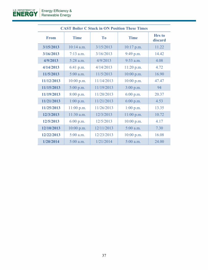
Appendix A Table 21. Periods in Which One of the Boilers in Building 3 Was Running Uncontrollably
CAST Boiler C Stuck in ON Position These Times
From Time To Time Hours to Discard
11/6/2012 8:30 a.m. 11/6/2012 9:04 p.m. 11.97
11/9/2012 9:48 a.m. 11/9/2012 5:15 p.m. 7.08
11/17/2012 10:14 a.m. 11/17/2012 1:45 p.m. 3.07
11/19/2012 4:53 p.m. 11/19/2012 7:19 p.m. 1.87
11/25/2012 7:02 p.m. 11/25/2012 10:18 p.m. 2.85
11/26/2012 10:24 a.m. 11/26/2012 6:47 p.m. 8.30
12/23/2012 5:45 a.m. 12/23/2012 10:16 p.m. 16.40
12/28/2012 11:22 a.m. 12/30/2012 11:59 p.m. 60.73
12/30/2012 11:59 p.m. 12/31/2012 1:00 p.m. 12.72
1/1/2013 8:50 a.m. 1/1/2013 10:13 p.m. 13.20
1/2/2013 11:44 a.m. 1/2/2013 5:56 p.m. 6.28
1/4/2013 9:03 a.m. 1/4/2013 10:12 p.m. 13.65
1/8/2013 4:50 p.m. 1/8/2013 10:20 p.m. 5.57
1/10/2013 7:59 a.m. 1/10/2013 4:58 p.m. 8.75
1/19/2013 8:58 a.m. 1/19/2013 10:09 p.m. 13.05
1/20/2013 7:10 p.m. 1/20/2013 8:40 p.m. 1.55
1/28/2013 6:45 a.m. 1/28/2013 10:13 p.m. 16.22
2/1/2013 7:02 a.m. 2/1/2013 10:09 p.m. 15.13
2/4/2013 8:29 p.m. 2/4/2013 10:07 p.m. 1.78
2/6/2013 9:39 a.m. 2/6/2013 10:09 p.m. 12.50
2/8/2013 5:54 a.m. 2/8/2013 10:09 p.m. 16.28
2/17/2013 9:46 a.m. 2/17/2013 10:29 p.m. 13.47
2/19/2013 1:01 p.m. 2/19/2013 7:49 p.m. 6.05
2/25/2013 6:53 p.m. 2/25/2013 9:18 p.m. 2.08
2/28/2013 9:46 a.m. 2/28/2013 3:56 p.m. 6.20
3/1/2013 6:44 a.m. 3/4/2013 11:27 a.m. 76.30
3/6/2013 1:06 p.m. 3/6/2013 8:56 p.m. 7.57
37
CAST Boiler C Stuck in ON Position These Times
From Time To Time Hrs to discard
3/15/2013 10:14 a.m. 3/15/2013 10:17 p.m. 11.22
3/16/2013 7:13 a.m. 3/16/2013 9:49 p.m. 14.42
4/9/2013 5:28 a.m. 4/9/2013 9:53 a.m. 4.08
4/14/2013 6:41 p.m. 4/14/2013 11:20 p.m. 4.72
11/5/2013 5:00 a.m. 11/5/2013 10:00 p.m. 16.90
11/12/2013 10:00 p.m. 11/14/2013 10:00 p.m. 47.47
11/15/2013 5:00 p.m. 11/19/2013 3:00 p.m. 94
11/19/2013 8:00 p.m. 11/20/2013 6:00 p.m. 20.37
11/21/2013 1:00 p.m. 11/21/2013 6:00 p.m. 4.53
11/25/2013 11:00 p.m. 11/26/2013 1:00 p.m. 13.35
12/3/2013 11:30 a.m. 12/3/2013 11:00 p.m. 10.72
12/5/2013 6:00 p.m. 12/5/2013 10:00 p.m. 4.17
12/10/2013 10:00 p.m. 12/11/2013 5:00 a.m. 7.30
12/22/2013 5:00 a.m. 12/23/2013 10:00 p.m. 16.08
1/20/2014 5:00 a.m. 1/21/2014 5:00 a.m. 24.00
38
Appendix B
This appendix presents sample data freom each building, illustrating controller operation and effects.
Building 3 Figure 25 shows the system temperature for the three sample periods with Intech control in which different control settings were implemented:
• January 1 to February 16, 2012 (black crosses): During this period, ORC was not enabled. The system was operated with a fixed return water temperature that differed only during daytime (180°F) and nighttime (170°F) due to a nighttime setback. The two black horizontal groups of data points reflect these two system set points.
• February 17 to April 4, 2012 (red stars): ORC was enabled on February 17, 2012. The system temperatures are significantly lower during this period. However, because a number of other adjustments to controller settings were made during February and March, a clear trend line is not evident.
• April 5 to May 31, 2012 (blue diamonds): During this period, control settings were fixed and indoor cutoff was added. A trend line is evident, indicating the ORC. Many data points are at the bottom of the plot during this period because of the greater incidence of WWSD during this time of year.
Figure 26 shows the system temperature compared to the average indoor temperature from the apartment temperature sensors. The red data points (stars) are from the period prior to indoor cutoff; the blue data points (diamonds) are during indoor cutoff. The lack of blue data points to the right of approximately 74°F indoor temperature confirms that this function was operating: there is no boiler operation above 74°F average indoor temperature. Indoor temperature cutoff was set at 73°F during the day and 68°F at night, with a 1°F dead band.
Figure 27 and Figure 28 show the range and fluctuation of apartment temperatures with and without indoor cutoff activated.
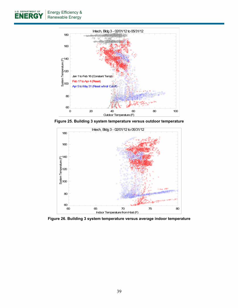
39
Figure 25. Building 3 system temperature versus outdoor temperature
Figure 26. Building 3 system temperature versus average indoor temperature
Intech, Bldg 3 - 02/01/12 to 05/31/12
0 20 40 60 80 100Outdoor Temperature (F)
60
80
100
120
140
160
180
Syste
m T
empe
ratu
re (F
)
Jan 1 to Feb 16 (Constant Temp)
Feb 17 to Apr 4 (Reset)
Apr 5 to May 31 (Reset w/Indr Cutoff)
Intech, Bldg 3 - 02/01/12 to 05/31/12
60 65 70 75 80Indoor Temperature from Host (F)
60
80
100
120
140
160
180
Syste
m T
empe
ratu
re (F
)
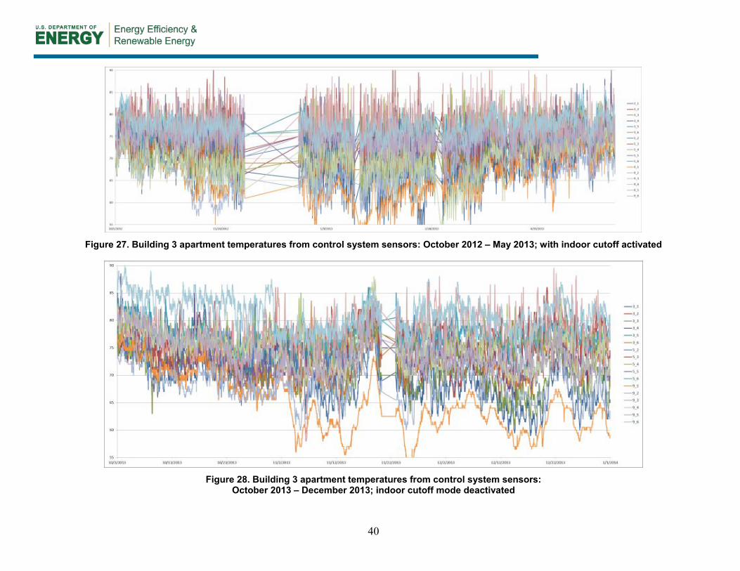
40
Figure 27. Building 3 apartment temperatures from control system sensors: October 2012 – May 2013; with indoor cutoff activated
Figure 28. Building 3 apartment temperatures from control system sensors:
October 2013 – December 2013; indoor cutoff mode deactivated
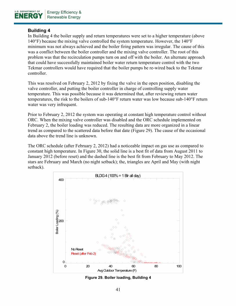
41
Building 4 In Building 4 the boiler supply and return temperatures were set to a higher temperature (above 140°F) because the mixing valve controlled the system temperature. However, the 140°F minimum was not always achieved and the boiler firing pattern was irregular. The cause of this was a conflict between the boiler controller and the mixing valve controller. The root of this problem was that the recirculation pumps turn on and off with the boiler. An alternate approach that could have successfully maintained boiler water return temperature control with the two Tekmar controllers would have required that the boiler pumps be re-wired back to the Tekmar controller.
This was resolved on February 2, 2012 by fixing the valve in the open position, disabling the valve controller, and putting the boiler controller in charge of controlling supply water temperature. This was possible because it was determined that, after reviewing return water temperatures, the risk to the boilers of sub-140°F return water was low because sub-140°F return water was very infrequent.
Prior to February 2, 2012 the system was operating at constant high temperature control without ORC. When the mixing valve controller was disabled and the ORC schedule implemented on February 2, the boiler loading was reduced. The resulting data are more organized in a linear trend as compared to the scattered data before that date (Figure 29). The cause of the occasional data above the trend line is unknown.
The ORC schedule (after February 2, 2012) had a noticeable impact on gas use as compared to constant high temperature. In Figure 30, the solid line is a best fit of data from August 2011 to January 2012 (before reset) and the dashed line is the best fit from February to May 2012. The stars are February and March (no night setback); the, triangles are April and May (with night setback).
Figure 29. Boiler loading, Building 4
BLDG 4 (100% = 1 Blr all day)
0 20 40 60 80 100Avg Outdoor Temperature (F)
0
200
400
Boile
r Loa
ding
(%)
Reset (after Feb 2)No Reset

42
Figure 30. Gas use, Building 4
Nighttime Setback Nighttime setback was implemented in March. There was little evidence of the 5°F nighttime setback having an impact on boiler runtime. Both the days with and the days without setback fall roughly along the same boiler loading trend line (Figure 31).
Figure 31. No impact of nighttime setback, Building 4
20 40 60 80Outdoor Temperature (F)
0
10
20
30
40
50
Gas U
se (t
herm
s/day
)
BLDG 4 (100% = 1 Blr all day)
0 20 40 60 80 100Avg Outdoor Temperature (F)
0
50
100
150
Boile
r Loa
ding
(%)
Reset (after Feb 2)
Reset & Setback
Aug-11 to Jan-12 Feb-12 & Mar-12
Apr-12 & May-12
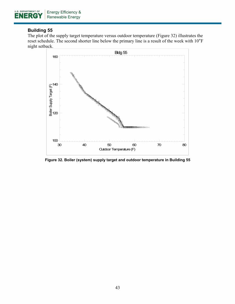
43
Building 55 The plot of the supply target temperature versus outdoor temperature (Figure 32) illustrates the reset schedule. The second shorter line below the primary line is a result of the week with 10°F night setback.
Figure 32. Boiler (system) supply target and outdoor temperature in Building 55
Bldg 55
30 40 50 60 70 80Outdoor Temperature (F)
100
120
140
160
Boile
r Sup
ply T
arge
t (F)

DOE/GO-102014-4493 ▪ September 2014