Prof. Dr. Paolo Burlando Chair of Hydrology and Water Resources Management

Hydrology -Collection of formulas-

(Aid for the Exam and the Assignments)

Zurich, 2011

Remark This formulary is meant to be of assistance in working on the exam and the exercises. The concepts which stand behind the here mentioned formulas are explained in the lecture and the recommended literature. The students should be able to understand and to reproduce them.

1/19

1. Hydrologic Processes

1.1. Precipitation Synthetic hyetographs

Triangular hyetograph:

/ 0

( )

0

d a a

d d da d

b b

d

i t t t ti T i ti t t t T

t tt T

≤ ≤

⋅= − ≤ ≤ >

0.3...0.48a

d

trT

= .

[L/T]

[-]

Alternating block method:

1

1

n

n n n jj

P i T P−

=

= ⋅ −∑

[L]

1.2. Runoff

H-Q-relationship: ( )nQ a H b= − [L3/T]

Mean square error: 2

( )1

11001

nj j

Q Hj j

Q Qm

n Q=

−= −

∑ [L3/T]

Hydrograph analysis

Recession curve: 0( )/0( ) t t RQ t Q e− −= ⋅ [L3/T]

2/19

1.3. Evaporation from Water Bodies Aerodynamic or Dalton-Method

Evaporation: ( ) ( ( ) )W sE f v e T e= ⋅ − (mm/d)

Saturated Vapour Pressure (Magnus Formula):

17.62( ) 6.122 exp243.12s

Te TT

⋅ = ⋅ +

T (°C)

(hPa)

Wind function (2 m above ground): ( ) cf v a b v= + ⋅

v (m/s)

(mm/(d hPa))

Parameter after WMO-guideline: 0.13 0.094 1.0a b c= = =

Vapour Pressure of the air: ( )100srHe e T= ⋅ (hPa)

Penman-Method

Evaporation: / ( ) ( ( ) )n s

wR L f v e T eE γ

γ∆ ⋅ + ⋅ ⋅ −

=∆ +

(mm/d)

Psychrometer Constant: 0.67γ ≈ hPa/K

Heat of evaporation at 20°C: 28.3L = W d m-2 mm-1

Slope of the Saturation Vapour Pressure Curve: 2

4284( )(243.12 )

ss

e e TT T∂

∆ = = ⋅∂ +

T (°C)

(hPa/K)

3/19

1.4. Evaporation from Land Surfaces

Thornthwaite

Potential Evapotranspiration: 10

16a

jj j

TPET b

I⋅

= ⋅ ⋅

(mm/month)

Coefficient: 1.6 0.5100

a I= +

Thermal annual index:

1.51412

1 5j

j

TI

=

=

∑

T (°C)

Coefficient b depending on month and latitude: 12 30

=

L Nb

N Number of days per month

[-]

Daily sunshine duration: 12.3 4.3 0.167 ( 51)

( )= + ⋅ + ⋅ ⋅ −°

L ς ς ϕϕ

(h)

sin[ (2 / 365) 1.39]DOY

DOYς π= −

Day of the year

Penman method

Potential Evapotranspiration: r aE EPET γγ

∆ ⋅ + ⋅=

∆ + (mm/d)

Evaporation equivalent of the global radiation:

0.6 Gr

REL⋅

=

GR (Wm-2) L ( W d m-2 mm-1)

(mm/d)

Ventilation term: 20.063 (1 1.08 ) ( ( ) )a s RE v e T e S= ⋅ + ⋅ ⋅ − ⋅

2v (m/s) RS (-)

(mm/d)

4/19

Evapotranspiration for different vegetation cover

Potential Evapotranspiration: c grasPET f PET= ⋅ [L/T]

Table 1 Crop factor fc for different vegetation cover and seasons

Vegetation Mar Apr May Jun Jul Aug Sep Oct Nov to Feb

mowing meadow 1.00 1.00 1.05 1.10 1.10 1.05 1.05 1.00 1.00 winter wheat 0.90 0.95 1.15 1.35 1.30 1.00 - - 0.65 spring barley - 0.75 1.30 1.40 1.30 - - - - sugar beets - 0.50 0.75 1.10 1.30 1.25 1.10 0.85 - potatoes - 0.50 0.90 1.10 1.40 1.20 0.90 - -

1.5. Infiltration and Net Precipitation

Richard‘s Equation (1D): fD kt z zθ θ∂ ∂ ∂ = + ∂ ∂ ∂ [1/T]

Darcy‘s law: fhq kz∂

= −∂ [L/T]

Continuity equation: 0qt zθ∂ ∂+ =

∂ ∂ [1/T]

Soil moisture content: Wasser

Gesamt

VV

θ = [-]

Momentum equation: fq k Dzθ∂ = − + ∂ [L/T]

Soil water diffusivity: fdD kdψθ

= [L2/T]

Suction head: h zψ = − [L]

5/19

Horton’s equation

Potential infiltration rate: 0( ) ( ) ktc cf t f f f e−= + − [L/T]

Potential cumulative infiltration: 0( ) (1 )ktcc

f fF t f t ek

−−= ⋅ + − [L]

Ponding time under constant rainfall intensity i:

00

0

1 ln cp c

c

c

f ft f i fi k i f

f i f

−= − + ⋅ − < <

[T]

Equivalent time origin for potential infiltration after ponding:

00

1 ln cp

c

f ft tk i f

−= − −

[T]

Infiltration rate after ponding: 0( )0( ) ( ) k t t

c cf t f f f e− −= + − [L/T]

Cumulative infiltration after ponding:

0( )00( ) ( ) (1 )k t tc

cf fF t f t t e

k− −−

= ⋅ − + − [L]

SCS-CN-Method

Cumulative rainfall excess (actual runoff):

2

max

[ ( ) ]( )[ ( ) ]

ae

a

P t IP tP t I S

−=

− +

[L]

( ) afor P t I> P(t)…cumulative precipitation

Potential maximum retention: max 0

0 max

1000 -10

25.4 if S in mm

S SCN

S

=

= [L]

Equivalent curve numbers for dry (I) or wet(II) antecedent moisture conditions:

4.210 0.058

2310 0.13

III

II

IIIII

II

CNCNCN

CNCNCN

⋅=

−⋅

=+

[-]

6/19

Table 2 Classification of hydrologic soil groups [source: Maidment, 1992]

Hydrologic Soil Group Description A Soils with high infiltration rates even when thoroughly wetted

e.g. deep sand or gravel B Soils with moderate infiltration rates when thoroughly wetted,

moderately deep to deep soils, with moderately fine to moderately coarse texture e.g. moderate deep sands, loess

C Soils with low infiltration rates when thoroughly wetted, moderately fine to fine texture or a layer that impedes downward movement of water e.g. shallow sandy loam, sandy clay loam

D Soils with very low infiltration rates when thoroughly wetted, and high runoff potential, swell significantly when wet e.g. clay

Table 3 Classification of antecedent moisture classes (AMC) [source: SCS, 1972]

Total 5 – day antecedent rainfall (mm) AMC group Dormant season Growing season

I 12.7P < 35.6P < II 12.7 27.9P≤ < 35.6 53.3P≤ < III 27.9P ≥ 53.3P ≥

Table 4 Curve numbers for AMC group II [source: Maidment, 1992 and DVWK Regeln 113/1984]

Cover type CNII for hydrologic soil group A B C D

Fallow, bare soil 77 86 91 94

root and tuber crops, vine 70 80 87 90

Crops, forage crop 64 76 84 88

Pasture, grassland poor 68 79 86 89 fair 49 69 79 84

Meadow 30 58 71 78

Woods poor 45 66 77 83 fair 36 60 73 79 good 25 55 70 77

Urban areas with open space (lawns, parks, golf courses, cemeteries, etc.)

good condition (grass cover > 75%) 39 61 74 80 fair condition (grass cover 50 to 75 %) 49 69 79 84 poor condition (grass cover < 50%) 68 79 86 89

Impervious/sealed areas 100 100 100 100

7/19

2. Runoff Concentration / Unit Hydrograph

2.1. Application

Convolution integral: 0

( ) ( ) ( )t

q t p h t dt t t= ⋅ −∫

h [1/T]; t [T]

Discrete convolution: ( ) 11

n

m m i ii

q t p h t− +=

= ⋅ ⋅∆∑

h [1/T]; t [T]

dim q = dim p Attention! Convert to get Q in L3/T

2.2. Linear Reservoirs in Series (Nash-Cascade)

Pulse response function1: 1

/1( )( )

nt k

nth t e

k n k

−− = ⋅ ⋅Γ

[1/T]

Discrete version1: [ ] 1( 0.5) /( 0.5)

( )

nj t k

j n

j th e

k n

−− − ⋅∆− ⋅∆

= ⋅⋅Γ

[1/T]

Characteristics:

Time to peak: ( 1)Pt k n= − [T]

1. Moment/ time lag: 1h LM t k n= = ⋅ [T]

2. Moment/ variance: 22hM k n= ⋅ [T2]

Parameter estimation:

Relationship of moments in linear systems: m m mh Q IM M M= −

m: order of the moments h: transfer function Q: output function I: input function

[Tm]

1 Values for the Gamma function in Table A 2 (appendix)

8/19

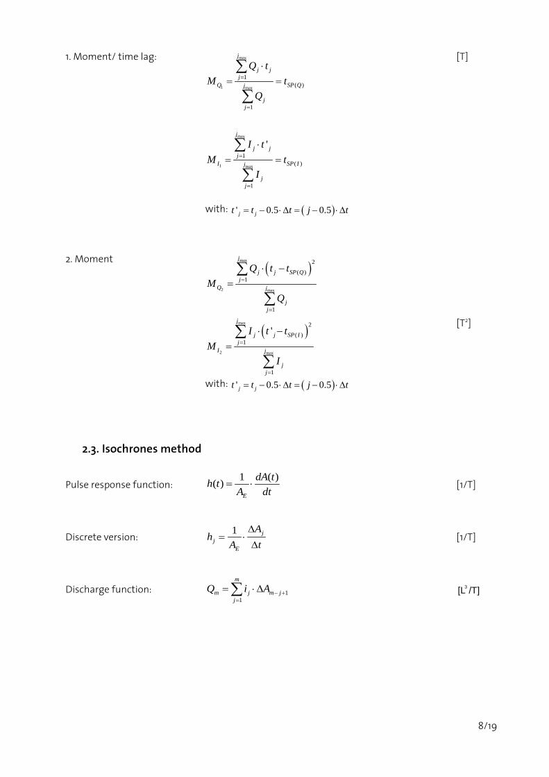
1. Moment/ time lag: max

1 max

max

1 max

1( )

1

1( )

1

'

j

j jj

Q SP Qj

jj

j

j jj

I SP Ij

jj

Q tM t

Q

I tM t

I

=

=

=

=

⋅= =

⋅= =

∑

∑

∑

∑ with: ( )' 0.5 0.5j jt t t j t= − ⋅∆ = − ⋅∆

[T]

2. Moment ( )

( )

max

2 max

max

2 max

2

( )1

1

2

( )1

1

'

j

j j SP Qj

Q j

jj

j

j j SP Ij

I j

jj

Q t tM

Q

I t tM

I

=

=

=

=

⋅ −=

⋅ −=

∑

∑

∑

∑

with: ( )' 0.5 0.5j jt t t j t= − ⋅∆ = − ⋅∆

[T2]

2.3. Isochrones method

Pulse response function: 1 ( )( )

E

dA th tA dt

= ⋅ [1/T]

Discrete version: 1 jj

E

Ah

A t∆

= ⋅∆ [1/T]

Discharge function: 11

m

m j m jj

Q i A − +=

= ⋅∆∑ 3[L /T]

9/19

2.4. Triangular Unit Hydrograph

/ 0

( )

0

p p p

p UH pp UH

UH p UH p

UH

h t t t th t h t

h t t t tt t t t

t t

≤ ≤

⋅= − ≤ ≤ − − >

[1/T]

Time lag: 1 ( )3L p UHt t t= + [T]

Base length: 2 /UH pt h= [T]

10/19

3. Probability and Statistics

3.1. Theoretical statistics of probability distributions

Mean / Expectation value: [ ] ( )

[ ] ( )i

x X

x i X ialle x

E X x f x dx

E X x p x

µ

µ

∞

−∞

= =

= =

∫

∑

continuous

discrete

Variance:

2 2

2 2

[ ] ( ) ( )

[ ] ( ) ( )i

x X X

x i X X ialle x

Var X x f x dx

Var X x p x

σ µ

σ µ

∞

−∞

= = −

= = −

∫

∑

continuous

discrete

Standard deviation: 1/2

2 2( ) ( ) ( )x x X Xx m f x dxσ σ∞

−∞

= = + −

∫

Skewness coefficient: 3

1 33 3

1 ( )( , )

n

ii X

X X

x xM Xn µγ

σ σ=

−= =

∑

Theoretical moments

General: ( ) [( ) ]rrM a E X a= −

Central moments for a µ=

1

( ) [( ) ] ( ) ( )

( ) [( ) ] ( ) ( )

r rr

nr r

r i ii

M E X x f x dx

M E X x f x

µ µ µ

µ µ µ

∞

−∞

=

= − = − ⋅

= − = − ⋅

∫

∑

continuous

discrete

12

2

3

( ) 0

( )( )

MMM

µ

µ σµ γ

=

==

Moments of origin for 0a =

1

(0) [ ] ( )

(0) [ ] ( )

r rr

nr r

r i ii

M E X x f x dx

M E X x f x

∞

−∞

=

= = ⋅

= = ⋅

∫

∑

continuous

discrete

11/19

3.2. Statistics of a sample

Arithmetic mean: 1

1 n

ii

x xn =

= ∑

Sample Variance: 2 2

1

1ˆ ( )1

n

ii

s x xn =

= −− ∑

Sample Standard deviation: 2 2

1

1ˆ ˆ ( )1

n

ii

s s x xn =

= = −− ∑

Sample Variation coefficient: ˆ

xsVx

=

Sample skewness coefficient: 33

1( )

ˆ( 1)( 2)

n

ii

n x xn n s

γ=

= −− − ∑

Sample moments

General: 1( )

( )

nr

ii

r

x bM b

n=

−=∑

Central moments for b x=

Moments of origin for 0b =

Correlation

Sample Covariance: 1

1 ( ) ( )1

n

xy i ii

s x x y yn =

= − ⋅ −− ∑

Sample correlation coefficient:

1

2 2

1 1

( ) ( )

( ) ( )

n

i ixy i

xy n nx y

i ii i

x x y ysr

s sx x y y

=

= =

− ⋅ −= =

⋅− ⋅ −

∑

∑ ∑

12/19

3.3. Sample Frequency Distributions / Plotting Position

Weibull: ( )1

iF xn

=+

Gringorten:

0.44( )0.12

iF xn−

=+

i … rank n … sample size

13/19

3.4. Probability distributions with continuous random variables

Table 5 Selection of probability distributions for fitting hydrologic data

Distribution Probability density function Distribution function Range Parameter estimation with the method of moments

Normal2 21 1( ) exp

22xf x µσσ π

− = −

( ) xF x µσ− = F

x−∞ ≤ ≤ ∞

, xx sµ σ= =

Log-Normal2

21 1( ) exp

22y

yy

yf x

xµ

σσ π

− = − mit lny x=

( ) y

y

yF x

µσ

−= F

0x >

2

2

ˆln(1 )

ln 0.5

xy

y y

sV Vx

x

σ

µ σ

= + =

= −

Exponential ( ) xf x e λλ −= ( ) 1 xF x e λ−= − 0x ≥ 1x

λ =

Gamma3

1

( , , )( )

r r xx ef x xr

λλλ− −

=Γ

mit Γ = Gammafunktion

1

0

( , , )( )

x r r tx eF x r dtr

λλλ− −

=Γ∫

000

x

rλ≥>>

2

2 2,x x

x xrs s

λ = =

Gumbel (Extreme value Type I)

1( ) exp expx u x uf xα α α

− − = − − − ( ) exp exp x uF x

α − = − −

x−∞ < < ∞ 6

xsαπ

=

0.5772u x α= − ⋅

2 Values for the standard normal distribution in Table A 1 (appendix) 3 Values for the Gamma function in Table A 2 (appendix)

14/19

3.5. Flood Statistics

Return Period: 1 1

1 U O

RF F

= =−

[years]

Standardized runoff: *

[ ]i

iHQHQ

E HQ= [-]

Relative risk: 11 1

L

rR

= − −

L (years)

[-]

3.6. Goodness-of-fit test

Kolmogorow – Smirnow – Test

Criterion:

1max { }nd i theor empT F F== −

Kolmogorow-Smirnow statistic4 :

( , )c n α

Null hypothesis H0: The sample has the assumed distribution.

0d

d

T cT c

α

α

< →

> → 0

Accept HReject H

4 Values in Table A 3 (appendix)

15/19

4. Erosion and Sediment Transport

4.1. Hillslope erosion

Universal Soil Loss Equation (U.S.L.E.) A R K L S C P= ⋅ ⋅ ⋅ ⋅ ⋅ (t/(ha a))

Erosivity-Index for the rainfall event: 30evR E I= ⋅

30I maximum 30-Minutes Intensity (mm/h)

((MJ mm)/ (ha h))

Energy associated individual rainfall event: ∆

= ⋅∑ r rtE e h

0.119 0.0 73 log 76mm/h0.283 76mm/h

e i ie i= + 8 ⋅ ≤= >

(MJ/ha)

(MJ/ha mm)

Annual – Erosivity - Index: ( )1

N

ev ii

R R=

=∑ ((MJ mm)/ (ha h))

Erodibility-Index: 7 1.14 3 32.77 10 (12 ) 4.3 10 ( 2) 3.3 10 ( 3)− − −= ⋅ − + ⋅ ⋅ − + ⋅ ⋅ −⋅K M a b c

1...41...6

==

bc

K (t ha-1 MJ-1 mm-1 ha h)

Parameter that considers soil particle size:

/ /Schluff Sand Schluff TonM α γ= ⋅(100 − )

(-)

16/19

4.2. Sediment transport

Bed shear stress: 0 w g R St ρ= ⋅ ⋅ ⋅ [M/(LT2)]

R hydraulic radius [L]

Slope: sin tanS α α= ≈ [°]

Bed shear stress (Meyer-Peter):

3/2

0 wr

kg R Sk

k

t ρ

= ⋅ ⋅ ⋅ ⋅

1/3 Strickler cofficient (m /s)

[M/(LT2)]

Grain roughness (Müller):

1/6

26r

m

m

kd

d

=

average grain size (m)

(m1/3/s)

Critical shear stress (Mayer-Peter and Müller): 0.047( )c s w mg dt ρ ρ= − ⋅ ⋅ [M/(LT2)]

Bed load transport: 3/200.5

8 ( )(1 / )s c

w w s

ggt t

ρ ρ ρ= −

− ⋅ [M/(LT)]

Shields’ parameter: 2

* *w

s w m

vg d

ρtρ ρ

= ⋅− ⋅

[-]

Shear velocity: * 0 /v t ρ= [L/T]

Reynolds number: **Re mv d

υ⋅

= [-]

Kinematic viscosity: µυρ

= [L2/T]

17/19

Appendix

Table A 1 Values of the standardized normal distribution ( ) 21 1exp22

z

z t dt−∞

F = − ∫

z 0.00 0.01 0.02 0.03 0.04 0.05 0.06 0.07 0.08 0.09

0.0 0.5000 0.5040 0.5080 0.5120 0.5160 0.5199 0.5239 0.5279 0.5319 0.5359

0.1 0.5398 0.5438 0.5478 0.5517 0.5557 0.5596 0.5636 0.5675 0.5714 0.5753

0.2 0.5793 0.5832 0.5871 0.5910 0.5948 0.5987 0.6026 0.6064 0.6103 0.6141

0.3 0.6179 0.6217 0.6255 0.6293 0.6331 0.6368 0.6406 0.6443 0.6480 0.6517

0.4 0.6554 0.6591 0.6628 0.6664 0.6700 0.6736 0.6772 0.6808 0.6844 0.6879

0.5 0.6915 0.6950 0.6985 0.7019 0.7054 0.7088 0.7123 0.7157 0.7190 0.7224

0.6 0.7257 0.7291 0.7324 0.7357 0.7389 0.7422 0.7454 0.7486 0.7517 0.7549

0.7 0.7580 0.7611 0.7642 0.7673 0.7704 0.7734 0.7764 0.7794 0.7823 0.7852

0.8 0.7881 0.7910 0.7939 0.7967 0.7995 0.8023 0.8051 0.8078 0.8106 0.8133

0.9 0.8159 0.8186 0.8212 0.8238 0.8264 0.8289 0.8315 0.8340 0.8365 0.8389

1.0 0.8413 0.8438 0.8461 0.8485 0.8508 0.8531 0.8554 0.8577 0.8599 0.8621

1.1 0.8643 0.8665 0.8686 0.8708 0.8729 0.8749 0.8770 0.8790 0.8810 0.8830

1.2 0.8849 0.8869 0.8888 0.8907 0.8925 0.8944 0.8962 0.8980 0.8997 0.9015

1.3 0.90320 0.90490 0.90658 0.90824 0.90988 0.91149 0.91309 0.91466 0.91621 0.91774

1.4 0.91924 0.92073 0.92220 0.92364 0.92507 0.92647 0.92785 0.92922 0.93056 0.93189

1.5 0.93319 0.93448 0.93574 0.93699 0.93822 0.93943 0.94062 0.94179 0.94295 0.94408

1.6 0.94520 0.94630 0.94738 0.94845 0.94950 0.95053 0.95154 0.95254 0.95352 0.95449

1.7 0.95543 0.95637 0.95728 0.95818 0.95907 0.95994 0.96080 0.96164 0.96246 0.96327

1.8 0.96407 0.96485 0.96562 0.96638 0.96712 0.96784 0.96856 0.96926 0.96995 0.97062

1.9 0.97128 0.97193 0.97257 0.97320 0.97381 0.97441 0.97500 0.97558 0.97615 0.97670

2.0 0.97725 0.977784 0.978308 0.978822 0.979325 0.979818 0.980301 0.980774 0.981237 0.981691

2.1 0.98214 0.982571 0.982997 0.983414 0.983823 0.984222 0.984614 0.984997 0.985371 0.985738

2.2 0.98610 0.986447 0.986791 0.987126 0.987455 0.987776 0.988089 0.988396 0.988696 0.988989

2.3 0.98928 0.989556 0.98983 0.990097 0.990358 0.990613 0.990863 0.991106 0.991344 0.991576

2.4 0.99180 0.992024 0.99224 0.992451 0.992656 0.992857 0.993053 0.993244 0.993431 0.993613

2.5 0.99379 0.993963 0.994132 0.994297 0.994457 0.994614 0.994766 0.994915 0.99506 0.995201

3.0 0.9986501 3.5 0.9997674 4.0 0.99996833 4.5 0.99999660 5.0 0.999999713 5.5 0.999999981

18/19

Table A 2 Values of the Gamma function for the interval 1 2α< ≤ :

α ( )αΓ α ( )αΓ α ( )αΓ α ( )αΓ α ( )αΓ

1.01 0.9943 1.21 0.9156 1.41 0.8868 1.61 0.8947 1.81 0.9341 1.02 0.9888 1.22 0.9131 1.42 0.8864 1.62 0.8959 1.82 0.9368 1.03 0.9835 1.23 0.9108 1.43 0.8860 1.63 0.8972 1.83 0.9397 1.04 0.9784 1.24 0.9085 1.44 0.8858 1.64 0.8986 1.84 0.9426 1.05 0.9735 1.25 0.9064 1.45 0.8857 1.65 0.9001 1.85 0.9456 1.06 0.9687 1.26 0.9044 1.46 0.8856 1.66 0.9017 1.86 0.9487 1.07 0.9642 1.27 0.9025 1.47 0.8856 1.67 0.9033 1.87 0.9518 1.08 0.9597 1.28 0.9007 1.48 0.8857 1.68 0.9050 1.88 0.9551 1.09 0.9555 1.29 0.8990 1.49 0.8859 1.69 0.9068 1.89 0.9584 1.10 0.9514 1.30 0.8975 1.50 0.8862 1.70 0.9086 1.90 0.9618 1.11 0.9474 1.31 0.8960 1.51 0.8866 1.71 0.9106 1.91 0.9652 1.12 0.9436 1.32 0.8946 1.52 0.8870 1.72 0.9126 1.92 0.9688 1.13 0.9399 1.33 0.8934 1.53 0.8876 1.73 0.9147 1.93 0.9724 1.14 0.9364 1.34 0.8922 1.54 0.8882 1.74 0.9168 1.94 0.9761 1.15 0.9330 1.35 0.8912 1.55 0.8889 1.75 0.9191 1.95 0.9799 1.16 0.9298 1.36 0.8902 1.56 0.8896 1.76 0.9214 1.96 0.9837 1.17 0.9267 1.37 0.8893 1.57 0.8905 1.77 0.9238 1.97 0.9877 1.18 0.9237 1.38 0.8885 1.58 0.8914 1.78 0.9262 1.98 0.9917 1.19 0.9209 1.39 0.8879 1.59 0.8924 1.79 0.9288 1.99 0.9958 1.20 0.9182 1.40 0.8873 1.60 0.8935 1.80 0.9314 2.00 1.0000

The values of the Gamma function for 2α > can be calculated by using Table A 2 and the following equation:

( ) ( )1α α αΓ + = ⋅Γ

Furthermore, for *α ∈ is ( ) ( )1 !α αΓ = −

19/19

Table A 3 Kolmogorow-Smirnow statistic ( ),c nα for the complete specified Kolmogorow-Smirnow test with level of significance α and sample size n

n 0.01α = 0.02α = 0.05α = 0.1α = 0.2α =

1 0.995 0.990 0.975 0.950 0.900 2 0.929 0.900 0.842 0.776 0.684 3 0.829 0.785 0.708 0.636 0.565 4 0.734 0.689 0.624 0.565 0.493 5 0.669 0.627 0.563 0.509 0.447 6 0.617 0.577 0.519 0.468 0.410 7 0.576 0.538 0.483 0.436 0.381 8 0.542 0.507 0.454 0.410 0.358 9 0.513 0.480 0.430 0.387 0.339

10 0.489 0.457 0.409 0.369 0.323 11 0.468 0.437 0.391 0.352 0.308 12 0.449 0.419 0.375 0.338 0.296 13 0.432 0.404 0.361 0.325 0.285 14 0.418 0.390 0.349 0.314 0.275 15 0.404 0.377 0.338 0.304 0.266 16 0.392 0.366 0.327 0.295 0.258 17 0.381 0.355 0.318 0.286 0.250 18 0.371 0.346 0.309 0.279 0.244 19 0.361 0.337 0.301 0.271 0.237

20 0.352 0.329 0.294 0.265 0.232 21 0.344 0.321 0.287 0.259 0.226 22 0.337 0.314 0.281 0.253 0.221 23 0.330 0.307 0.275 0.247 0.216 24 0.323 0.301 0.269 0.242 0.212 25 0.317 0.295 0.264 0.238 0.208 26 0.311 0.290 0.259 0.233 0.204 27 0.305 0.284 0.254 0.229 0.200 28 0.300 0.279 0.250 0.225 0.197 29 0.295 0.275 0.246 0.221 0.193

30 0.290 0.270 0.242 0.218 0.190 31 0.285 0.266 0.238 0.214 0.187 32 0.281 0.262 0.234 0.211 0.184 33 0.277 0.258 0.231 0.208 0.182 34 0.273 0.254 0.227 0.205 0.179 35 0.269 0.251 0.224 0.202 0.177 36 0.265 0.247 0.221 0.199 0.174 37 0.262 0.244 0.218 0.196 0.172 38 0.255 0.241 0.215 0.194 0.170 39 0.252 0.238 0.213 0.191 0.168 40 0.249 0.235 0.210 0.189 0.165

n > 40 1.63 / n 1.52 / n 1.36 / n 1.22 / n 1.07 / n