Research Report 125

Hydrologic Modeling of Landscape Functions of Wetlands

by Misganaw Demissie, Abiola A. Akanbi, and Abdul Khan

ILLINOIS STATE WATER SURVEY DEPARTMENT OF NATURAL RESOURCES

1997

Research Report 125

Hydrologic Modeling of Landscape Functions of Wetlands

by

Misganaw Demissie, Abiola A. Akanbi, and Abdul Khan

Title: Hydrologic Modeling of Landscape Functions of Wetlands

Abstract: An extensive literature review of existing hydrologic and hydraulic models has been conducted to select a mathematical model suitable for simulating the dynamic processes of wetlands and their impact on the hydrologic responses of the watershed containing the wetlands. Due to the lack of a single suitable model, a base model was developed by incorporating watershed and channel-routing components from two of the reviewed models. This physically based, distributed-parameter model has been tested and applied to one of the selected test watersheds in Illinois to evaluate the impact of wetlands on the watershed hydrology. The simulation results indicate that the peakflow reduction due to the presence of wetlands is significant for wetland areas of up to 60 percent of the watershed area. The reduction in peakflow was observed to diminish with distance downstream of the wetland outlet, indicating that the influence of the wetlands decreases as the distance from the wetland increases. The model results cannot be generalized for other watersheds until the model has been tested and verified for several watersheds in different parts of Illinois.

Reference: Demissie, Misganaw, Abiola A. Akanbi, and Abdul Khan. Hydrologic Mod­eling of Landscape Functions of Wetlands. Illinois State Water Survey, Champaign, Research Report 125, 1997.

Indexing Terms: Wetland, watershed, hydrology, hydraulics, model, channel routing, ground water, baseflow, peakflow, discharge, hydrograph, drainage, mathematical model, hydrologic function, wetland function, overland flow

STATE OF ILLINOIS HON. JIM EDGAR, Governor

DEPARTMENT OF NATURAL RESOURCES Brent Manning, Director

BOARD OF NATURAL RESOURCES AND CONSERVATION

Richard C. Alkire, Ph.D. University of Illinois at Urbana-Champaign Robert H. Benton, B.S.C.E., P.E., Engineering Benton and Associates, Inc. H.S. Gutowsky, Ph.D., Chemistry University of Illinois at Urbana-Champaign Jack Kahn, Ph.D., Geological Sciences Museum of Science and Industry Brent Manning, M.S., Zoology, Chair John Mead, J.D., Law Southern Illinois University at Carbondale Robert L. Metcalf, Ph.D., Biology University of Illinois at Urbana-Champaign Allan S. Mickelson, B.S., Forestry University of Illinois at Urbana-Champaign

ILLINOIS STATE WATER SURVEY Derek Winstanley, Chief, D. Phil., Oxford University

2204 GRIFFITH DRIVE CHAMPAIGN, ILLINOIS 61820-7495

1997

The Illinois Department of Natural Resources does not discriminate based upon race, color, national origin, age, sex, religion or disability in its programs, services, activities and facilities If you believe that you have been discriminated against or if you wish additional information, please contact the Department at (217) 785-0067 or the US. Department of the Interior Office of Equal Employment, Washington, DC. 20240.

This report was printed on recycled and recyclable papers.

Printed by authority of the State of Illinois (12-97-100)

CONTENTS Page

Abstract 1 Introduction 2

Objectives and Procedures 2 Acknowledgments 2

A Survey of Hydrologic Mathematical Models 3 Watershed Models 3

Lumped-Parameter Models 3 Distributed-Parameter Models 7 Depressional Watershed Models 10

Channel Routing 13

Criteria for Selecting Models/Model Components 16 Watershed Modeling Criteria 16 Channel-Routing Criteria 17

Model Formulation 18 Selection of Watershed Model and Its Components 18

Choice of the Base Model 18 Selection of Hydrologic Process Models 18

Selection of Channel-Routing Component 19 Actual Modifications Implemented in the Current Model 19

Model Development 21 Watershed Model Components 21

Interception 21 Depression Storage 21 Infiltration 22 Subsurface Drainage 23 Tile Drainage 24 Baseflow 24 Overland Flow 24 Tributary Channel Flow 25 Overland and Channel Flow Routing 25

Channel-Routing Component 27 Unsteady-Flow Equations 27 Finite Difference Solution 28

Coupling of Model Components 30

Model Testing 32 Parameter Sensitivity Analysis 32 Model Calibration 33

Soil Infiltration/Drainage Parameters 34 Ground-Water Release Constants 35 Surface Storage/Roughness Parameters 35 Channel Roughness Coefficient 35

Wetland Hydrology and Watershed Responses 37 Representation of Wetland Characteristics 37 Influence of Wetlands on Watershed Hydrologic Responses 38

Summary and Conclusions 39

References 40

LIST OF FIGURES Page

Figure 1. General form of the Stanford Watershed Model or SWM (after Crawford and Linsley, 1966) 4

Figure 2. General structure of the U.S. Department of Agriculture Hydrograph Laboratory-74 (USDAHL-74) model (after Holtan et al., 1975) 4

Figure 3. General form of the Streamflow Synthesis and Reservoir Regulation (SSARR) model (after U.S. Army Corps of Engineers, 1972a) 5

Figure 4. Generalized flow chart of the Storm Water Management Model or SWMM (after Lager et al., 1971) 5

Figure 5. General structure of me TR-20 model (after Soil Conservation Service, 1973) 5 Figure 6. Flow chart representation of the Hydrologic Engineering Center-1 (HEC-1) model

(after U.S. Army Corps of Engineers, 1985) 6 Figure 7. Generalized flow chart of the Chemicals, Runoff, and Erosion from Agricultural

Management Systems (CREAMS) model (after U.S. Department of Agriculture, 1980) 6 Figure 8. Conceptual representation of the SHE model (after Abbott et al., 1986) 7 Figure 9. Square grid network in the Areal Nonpoint Source Watershed Environment

Response Simulation (ANSWERS) model (after Beasley, 1977) 8 Figure 10. Components of the PACE Watershed Model or PWM (after Durgunoglu et al., 1987) 8 Figure 11. Watershed segmentation in the Variable Source Area Simulator 2 (VSAS2) 9 Figure 12. Schematic representation of the Institute of Hydrology Distributed Model or IHDM

(after Rogers et al., 1985) 10 Figure 13. Conceptualization of surface and subsurface drainage in the Iowa State University

Hydrologic Model or ISUHM (after Moore and Larson, 1979) 11 Figure 14. Schematic representation of the DRAINMOD model (after Skaggs, 1980) 12 Figure 15. Conceptual representation of channel flow in wetlands 14 Figure 16. Ground surface topographical profile used to derive surface storage relations 21 Figure 17. Distribution of infiltration capacity with soil moisture 23 Figure 18. Schematic diagram of subsurface drainage 24 Figure 19. Depth-runoff relations for overland flow 24 Figure 20. Horizontal and vertical components of discharge 26 Figure 21. Piecewise linear segmented curve approximation for Manning equation 27 Figure 22. Control volume in a channel reach 27 Figure 23. The four-point scheme for finite difference discretization 28 Figure 24. Wetland hydrologic model 31 Figure 25. Cypress Creek watershed in Lower Cache River basin 32 Figure 26. Discretization of Cypress Creek watershed 32 Figure 27. Variation of peakflow and time-to-peakflow to changes in a) ASM, b) Gf' c) hu,

d) rc, e) DF, f) DC, g) no, h) nc, i) fc, and j) A 33 Figure 28. Influence of a) ASM and b) DC on flood hydrograph 35 Figure 29. Comparison of computed and measured hydrographs for Cypress Creek for three storms:

a) 2/2/89, b) 1/19/90, and c) 5/13/90 36 Figure 30. Comparison of discharge hydrographs for different percent wedand at the watershed outlet 38 Figure 31. Variation of relative peakflow with increasing percent wetland at the watershed outlet 38

LIST OF TABLES

Page

Table 1. Hydrologic Model Characteristics (After Shafer and Skaggs, 1983) 13 Table 2. Model Channel-Routing Capabilities (After Eichert, 1970) 15 Table 3. Potential Interception Values (After Beasley and Huggins, 1982) 21 Table 4. Surface Storage and Roughness Parameters (Adapted from Beasley and Huggins, 1982) 22 Table 5. Typical Values of Soil Infiltration and Drainage Parameters

(Adapted from Beasley and Huggins, 1982) 23 Table 6. Range of Parameters for Sensitivity Analysis 33 Table 7. Calibration of Infiltration and Ground-Water Release Parameters 34 Table 8. Typical Values of Parameters for both Wetland and Nonwetland Areas 38

HYDROLOGIC MODELING OF LANDSCAPE FUNCTIONS OF WETLANDS

by Misganaw Demissie, Abiola A. Akanbi, and Abdul Khan

ABSTRACT

An extensive literature review of existing hydrologic and hydraulic models has been conducted to select a mathematical model suitable for simulating the dynamic processes of wetlands and their impact on the hydrologic responses of the watershed containing the wetlands. Due to the lack of a single suitable model, a base model was developed by incorporating watershed and channel-routing components from two of the reviewed models. This physically based, distributed-parameter model has been tested and applied to one of the selected test watersheds in Illinois to evaluate the impact of wetlands on the watershed hydrology. The simulation results indicate that the peakflow reduction due to the presence of wetlands is significant for wetland areas of up to 60 percent of the watershed area. The reduction in peakflow was observed to diminish with distance downstream of the wetland outlet, indicating that the influence of the wetlands decreases as the distance from the wetland increases. The model results cannot be generalized for other watersheds until the model has been tested and verified for several watersheds in different parts of Illinois.

1

INTRODUCTION

Hydrology is the primary driving force in wetland dynamics. Even though plant species and soil characteristics are generally used to identify wetlands, the dominant feature is the presence of excess water either on or beneath the land surface. The existence of any wetland depends on how wet the soil is, how long the area remains inundated by water, or both. The amount of water available in a wetland area at different times and the way the water moves in and out of the area are defined by the hydrology of the area and the hydraulics of flow, respectively. When the existing hydrologic regime is altered, the nature and functions of wetlands are also altered.

When rehabilitating, restoring, or creating wetlands, an attempt is made to imitate nature and provide the necessary hydrologic environment for the desired wetland type. Experience shows that it is difficult to successfully reproduce wetland hydrology. This is due to our limited understanding of wetland hydrology and its interrelation with the prevailing hydrologic conditions. Therefore, there is a great need for an improved understanding of the hydrologic characteristics and influences of different types of wetlands.

Mathematical models are an effective technique for evaluating the hydrologic characteristics and impacts of wetlands in detail. However, most existing hydrologic and hydraulic models were not designed to assess the hydrologic role of wetlands on landscape functions, but rather to fulfill other general hydrologic and hydraulic objectives. Consequently, these models do not address wetlands and their effects on the hydrologic processes in sufficient detail. In fact, the vast majority of the currently available models are not readily applicable for simulations of the hydrologic consequences of wetlands.

As a result, there is a great need for a mathematical model that considers the special wetland characteristics and thus is readily applicable for evaluating the hydrologic functions of wetlands. This project was designed to satisfy that need by developing a hydrologic model that is specially applicable for the evaluation of wetland functions and their impact on watershed hydrology.

Objectives and Procedures The main objectives of this project were: • To develop a physically based hydrologic and

hydraulic model that can be used to evaluate the cumulative hydrologic effects of wetlands in watersheds.

• To formulate the relations useful in estimating the influence of wetlands on the hydrologic responses of individual watersheds. These relations were developed on the basis of simulation runs made with the new model.

The following procedures were established to review and select appropriate model components and modeling tech­niques consistent with the specific objectives of the project: 1) Conduct an extensive literature review to compile a

list of existing hydrologic models for review and evaluation.

2) Develop criteria for selecting components for the proposed model from existing models.

3) Select from existing models those components and modeling approaches that are best suited to wetland hydrology.

4) Develop appropriate components if they are unavailable from existing models.

5) Assemble the developed components along with those derived from existing models and build a complete wetland hydrologic model.

6) Calibrate the new model using precipitation and streamflow data for three watersheds in Illinois.

7) Verify the model by using data (other than those used for calibration) from the same three watersheds.

8) Apply the model in simulations designed to answer questions related to hydrologic influences of wetlands in different watersheds. Model runs were made by using variable watershed

and channel parameters (such as land cover, infiltration rates, and channel roughness) that are influenced by the presence and absence of wetlands. The results will be used to develop relations between the hydrologic responses (such as peak flood, time to peak, runoff volume, and flood elevations) and the watershed and channel parameters.

The work performed in this study includes a thorough review of existing hydrologic models, development of criteria for selecting model components for the new model from existing models, development of the wetland hydrologic model, and model calibration and application to measure the impact of wetland alterations on the hydrologic responses of a watershed.

Acknowledgments This study was accomplished as part of the regular work

of the Illinois State Water Survey. The work was supported in part by funds provided by the Illinois Department of Conservation (IDOC). Marvin Hubbell, project manager for IDOC, has provided valuable guidance for this project. Water Survey staff members Laura Keefer and Radwan Al-Weshah provided assistance during different phases of the project. Kalpesh Patel, a graduate student in civil engineering at the University of Illinois, prepared most of the data. Becky Howard typed the report, Eva Kingston and Sarah Hibbeler edited the report, Linda Hascall prepared the graphics, and Linda Hascall and Becky Howard formatted the report.

2

A SURVEY OF HYDROLOGIC MATHEMATICAL MODELS

To develop a mathematical model for wetland hydrology, it is initially worthwhile to investigate and assess the capabilities of existing hydrologic watershed models. A watershed model is a complete hydrologic model designed to simulate the hydrologic response of a watershed under different climatic and landscape scenarios. It is developed by combining several submodels, each of which represents a hydrologic process. These process models include models for interception, evapotranspiration, infiltration, overland flow, subsurface flow, and channel routing.

The subsequent discussion focuses on two components of the hydrologic model for a watershed. The watershed component comprises all the hydrologic processes mentioned previously. Although this component incorporates channel routing, the differentiation of the channel-routing process into a separate component provides the means to obtain a more detailed channel-routing capability for the complete hydrologic model if and when necessary.

Watershed Models Mathematical hydrologic watershed models can be classi­

fied in various ways depending on important characteristics. Major classifications of models generally include four cat­egories: deterministic or stochastic models; empirical, phys­ically based, or conceptual models; lumped-parameter or distributed-parameter models; and continuous or event models.

Deterministic or stochastic model. Whether a model is classified as deterministic or stochastic depends on whether the randomness in its parameters is excluded or included. Thus a deterministic modeling approach does not consider the randomness that may be present as a result of uncertainties in the model parameters, while stochastic models do account for this randomness.

Empirical, physically based, or conceptual model. Whether a model is classified as empirical, physically based, or conceptual depends on how it represents important physical processes. An empirical model represents the dependence of the hydrologic system's output to input by a simple relationship usually devoid of any physical basis and often given in terms of an explicit, algebraic equation. A physically based model is formulated on the basis of well-established laws of physics, such as the conservation of mass, momentum, and energy. A conceptual model is an intermediate stage between empirical and physically based models. It represents the hydrologic system in terms of a number of elements, which are themselves simplified representations of the relevant physical processes. A physically based model has advantages over empirical and conceptual models in that its parameters can be measured or calculated from the watershed's observable physical, vegetative, land-use, and soil characteristics, whereas the parameters for the other two models have to be obtained through calibration and regionalization.

Lumped-parameter or distributed-parameter model. Whether a model is classified as lumped-parameter or distributed-parameter depends on how it determines and specifies the different model parameters. Variations in hydrologic response due to variations in rainfall, topography, vegetation, soil, and land use are assumed to be small in a lumped-parameter model, and thus the associated model parameters are represented by an average value. A distributed-parameter model, however, incorporates the differences in model parameters over small areas so that variations in hydrologic response due to small parameter changes can be simulated.

Continuous or event model. Whether a model is classified as a continuous or an event model depends on its temporal operation. A continuous model can sequentially simulate the hydrologic processes for an extended period before and after a storm event, taking into consideration the soil moisture storage recovery during dry periods. An event model, on the other hand, is designed to simulate the runoff process for one storm event at a time.

Several authors (Fleming, 1975; Chu and Bowers, 1977; Linsley, 1982; Shafer and Skaggs, 1983) have provided extensive reviews of available watershed models over the years. In the following sections, brief reviews of important watershed models are presented. Not every model cited in the literature has been included, nor have all the models in use today been reviewed. Most of the major watershed models relevant to wetland hydrology are discussed, however. To simplify the discussion, the models have been grouped into three major categories: lumped-parameter models, distributed-parameter models, and depressional watershed models. Only deterministic models are considered. The depressional watershed models included in the review are special lumped-parameter models developed for depressional watersheds as well as to simulate wetland drainage.

Lumped-Parameter Models

The earliest version of a complete watershed model is the Stanford Watershed Model (SWM) developed by Crawford and Linsley (1966) in California at Stanford University's Civil Engineering Department. This conceptual, lumped-parameter, continuous model uses variable time steps and is applicable for large, rural watersheds as well as urban watersheds. Most major hydrologic processes have been included in the SWM for which the general form is presented in figure 1. Interception is modeled as an initial abstraction from precipitation limited to a preset maximum. Evapotranspiration is calculated from the daily potential evapotranspiration value. Infiltration is modeled by an empirical equation. Overland flow is modeled by combining the continuity equation with the Manning equation. Interflow (quick subsurface flow) is simulated as a fraction

3

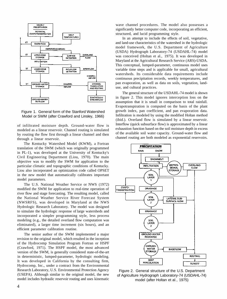
Figure 1. General form of the Stanford Watershed Model or SWM (after Crawford and Linsley, 1966)

of infiltrated moisture depth. Ground-water flow is modeled as a linear reservoir. Channel routing is simulated by routing the flow first through a linear channel and then through a linear reservoir.

The Kentucky Watershed Model (KWM), a Fortran translation of the SWM (which was originally programmed in PL-1), was developed at the University of Kentucky's Civil Engineering Department (Liou, 1970). The main objective was to modify the SWM for application to the particular climatic and topographic conditions of Kentucky. Liou also incorporated an optimization code called OPSET in the new model that automatically calibrates important model parameters.

The U.S. National Weather Service or NWS (1972) modified the SWM for application to real-time operation of river flow and stage forecasting. The resulting model, called the National Weather Service River Forecast System (NWSRFS), was developed in Maryland at the NWS Hydrologic Research Laboratory. The model was designed to simulate the hydrologic response of large watersheds and incorporated a simpler programming style, less process modeling (e.g., the detailed overland flow computation was eliminated), a larger time increment (six hours), and an efficient parameter calibration routine.

The senior author of the SWM implemented a major revision to the original model, which resulted in the inception of the Hydrocomp Simulation Program Fortran or HSPF (Crawford, 1971). The HSPF model, the most advanced version of the SWM, is generally considered state-of-the-art in deterministic, lumped-parameter, hydrologic modeling. It was developed in California by the consulting firm, Hydrocomp, Inc., under a contract from the Environmental Research Laboratory, U.S. Environmental Protection Agency (USEPA). Although similar to the original model, the new model includes hydraulic reservoir routing and uses kinematic

wave channel procedures. The model also possesses a significantly better computer code, incorporating an efficient, structured, and lucid programming style.

In an attempt to include the effects of soil, vegetative, and land-use characteristics of the watershed in the hydrologic model framework, the U.S. Department of Agriculture (USDA) Hydrograph Laboratory-74 (USDAHL-74) model was conceived (Holtan et al., 1975). It was developed in Maryland at the Agricultural Research Service (ARS)-USDA. This conceptual, lumped-parameter, continuous model uses variable time steps and is applicable for small, agricultural watersheds. Its considerable data requirements include continuous precipitation records, weekly temperatures, and pan evaporation, as well as data on soils, vegetation, land-use, and cultural practices.

The general structure of the USDAHL-74 model is shown in figure 2. This model ignores interception loss on the assumption that it is small in comparison to total rainfall. Evapotranspiration is computed on the basis of the plant growth index, pan coefficient, and pan evaporation data. Infiltration is modeled by using the modified Holtan method (ibid.). Overland flow is simulated by a linear reservoir. Interflow (quick subsurface flow) is approximated by a linear exhaustion function based on the soil moisture depth in excess of the available soil water capacity. Ground-water flow and channel routing are both modeled as exponential reservoirs.

Figure 2. General structure of the U.S. Department of Agriculture Hydrograph Laboratory-74 (USDAHL-74)

model (after Holtan et al., 1975)

4

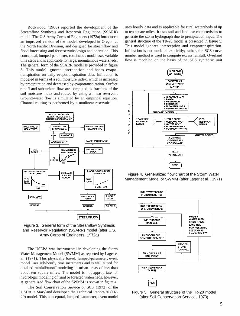
Rockwood (1968) reported the development of the Streamflow Synthesis and Reservoir Regulation (SSARR) model. The U.S Army Corps of Engineers (1972a) introduced an improved version of the model, developed in Oregon at the North Pacific Division, and designed for streamflow and flood forecasting and for reservoir design and operation. This conceptual, lumped-parameter, continuous model uses variable time steps and is applicable for large, mountainous watersheds. The general form of the SSARR model is provided in figure 3. This model ignores interception and bases evapo-transpiration on daily evapotranspiration data. Infiltration is modeled in terms of a soil moisture index, which is increased by precipitation and decreased by evapotranspiration. Surface runoff and subsurface flow are computed as fractions of the soil moisture index and routed by using a linear reservoir. Ground-water flow is simulated by an empirical equation. Channel routing is performed by a nonlinear reservoir.

Figure 3. General form of the Streamflow Synthesis and Reservoir Regulation (SSARR) model (after U.S.

Army Corps of Engineers, 1972a)

The USEPA was instrumental in developing the Storm Water Management Model (SWMM) as reported by Lager et al. (1971). This physically based, lumped-parameter, event model uses sub-hourly time increments and is well suited for detailed rainfall/runoff modeling in urban areas of less than about ten square miles. The model is not appropriate for hydrologic modeling of rural or forested watersheds, however. A generalized flow chart of the SWMM is shown in figure 4.

The Soil Conservation Service or SCS (1973) of the USDA in Maryland developed the Technical Report-20 (TR-20) model. This conceptual, lumped-parameter, event model

uses hourly data and is applicable for rural watersheds of up to ten square miles. It uses soil and land-use characteristics to generate the storm hydrograph due to precipitation input. The general structure of the TR-20 model is presented in figure 5. This model ignores interception and evapotranspiration. Infiltration is not modeled explicitly; rather, the SCS curve number method is used to compute excess rainfall. Overland flow is modeled on the basis of the SCS synthetic unit

Figure 4. Generalized flow chart of the Storm Water Management Model or SWMM (after Lager et al., 1971)

Figure 5. General structure of the TR-20 model (after Soil Conservation Service, 1973)

5

hydrograph method. Channel routing is performed by the CONVEX method, which is essentially a single-parameter Muskingum method (McCarthy, 1938). Ground-water flow is not simulated in this model.

One of the most widely used conceptual, lumped-parameter, event models is the HEC-1 flood hydrograph package (U.S. Army Corps of Engineers, 1985), which was developed in California at the Hydrologic Engineering Center. It uses variable time increments and is applicable for rural and urban watersheds of various sizes. A flow chart of the HEC-1 model is presented in figure 6. Interception, evapotranspiration, and infiltration are not generally modeled explicitly. Instead, these processes are together defined as abstraction from precipitation, which can be computed by various loss rate options, such as the uniform loss rate method, exponential loss function technique, and SCS curve number method. Besides these loss rate options, the modified Holtan infiltration technique (Holtan et al., 1975) is also available. The HEC-1 model incorporates different unit hydrograph methods to simulate surface flow. Among the different options available are the SCS method, Snyder's (1938) method, Clark's (1945) method, and a user-supplied unit hydrograph. Subsurface flow is not simulated. Ground-water flow is modeled as an exponential reservoir. Channel routing can be done by either the kinematic wave technique or the Muskingum method (McCarthy, 1938).

Figure 6. Flow chart representation of the Hydrologic Engineering Center-1 (HEC-1)

model (after U.S. Army Corps of Engineers, 1985)

The USDA (1980) developed a physically based, lumped-parameter, event model called the Chemicals, Runoff, and Erosion from Agricultural Management Systems (CREAMS) model to simulate the infiltration, evaporation, and percolation components of the hydrologic cycle. It was developed in Arizona at the Science and Education Administration, ARS-USDA. It uses daily or hourly data and is applicable for field-

scale sites of less than about 40 acres. A generalized flow chart of the CREAMS model is provided in figure 7. In this model, interception is ignored. Potential evapotranspiration is computed by the modified Penman (1948) equation, which uses daily temperature and solar radiation data. Actual evapotranspiration is calculated from potential evapo­transpiration, the leaf area index, and available soil water. For daily precipitation data, rainfall excess is computed on the basis of the SCS curve number technique unless hourly data are available. Then the model uses the Green-Ampt (1911) infiltration equation to compute rainfall excess. In this model, several layers of soil may be considered in the simulation of the soil moisture distribution, which enables a more accurate calculation of percolation. Surface flow is simulated by using the SCS unit hydrograph method, whereas interflow, ground­water flow, and channel routing are not modeled at all.

Figure 7. Generalized flow chart of the Chemicals, Runoff, and Erosion from Agricultural

Management Systems (CREAMS) model (after U.S. Department of Agriculture, 1980)

The Soil-Plant-Air-Water (SPAW) model (Saxton et al., 1984) was developed by the USDA. Although the model philosophy is similar to that of the CREAMS model, the SPAW model uses more physically based equations to mimic moisture movement in the soil and to account for the interaction between soil, water, and plant characteristics, such as the rooting depth and plant water stress. It uses the Darcy equation to redistribute moisture among the different soil layers.

6

Another model based on the CREAMS model, the Sim­ulator for Water Resources in Rural Basins or SWRRB model (Williams et al., 1985), was developed in Texas at the ARS-USDA. The original model was modified for application to large, rural basins by incorporating a channel-routing algorithm. The routing was accomplished by using a nonlinear reservoir. In addition, the model was changed to perform continuous simulation, and a component was added to simulate interflow.

Distributed-Parameter Models

Freeze (1971) developed a physically based, fully distributed, three-dimensional, saturated-unsaturated flow model in New York's IBM Thomas Watson Research Center. This continuous model uses sub-hourly data and is applicable for small, rural watersheds. It is one of the few models reported in the literature that uses completely coupled three-dimensional flow equations, which are solved by the finite-difference technique. Because of the complex model structure, massive input data requirements, and long computation time, however, it was tested only on a small hypothetical basin.

The European Hydrologic System (Systeme Hydro-logique Europeen, or SHE) model was cooperatively developed by the Danish Hydraulic Institute, the French

consulting company SOGREAH, and the British Institute of Hydrology (Abbott et al., 1986). This comprehensive, physically based, distributed-parameter, event model requires extensive data input and computing time. The watershed model simulates all the important physical processes including interception and evapotranspiration, overland flow and channel flow, and saturated and unsaturated subsurface flow. The model incorporates spatial variability of the hydrological parameters, inputs, and outputs by an orthogonal grid system (horizontal plane) and by columns of horizontal components at each grid section (vertical plane).

A conceptual representation of the different hydrologic processes and their interaction as modeled in the SHE model is presented in figure 8. Interception is simulated by using a method proposed by Rutter (Rutter et al., 1971), which is based on the equation of continuity of canopy storage and on func­tional relations between canopy storage capacity and several parameters, including leaf area index and evapotranspiration. Potential evapotranspiration is computed by the Penman-Monteith equation (Monteith, 1965) on the basis of such parameters as solar radiation and air density, specific heat, vapor pressure deficit, and latent heat of vaporization. Actual evapotranspiration is calculated as a linear function of potential evapotranspiration based on the soil moisture tension value.

Figure 8. Conceptual representation of the SHE model (after Abbott et al., 1986)

7

The processes of overland flow, channel flow, and saturated-unsaturated subsurface flow are modeled by using nonlinear partial differential equations of fluid flow, which are solved by finite-difference techniques. One-dimensional vertical unsaturated flow (infiltration) is modeled by the Richards (1931) equation. Two-dimensional planar overland flow (in the X-Y plane) is modeled by the diffusion wave approximation of the Saint-Venant equations. Channel routing is performed by the one-dimensional diffusion wave method. Two-dimensional planar saturated-unsaturated subsurface flow (ground-water flow) is simulated by using the Richards equation in the X-Y plane.

The SHE model uses sub-hourly data and in theory is applicable for rural and forested watersheds of various sizes and land uses. In practice, however, its use as an operational tool is restricted by several major impediments. These include massive information required as model input and high computing costs necessary to run the program.

Beasley (1977) developed a physically based, distributed-parameter, event model called the Areal Nonpoint Source Watershed Environment Response Simulation (ANSWERS) model. It was developed in Indiana at Purdue University's Agricultural Engineering Department. It uses sub-hourly time increments and is applicable for agricultural watersheds smaller than about 40 square miles. In this model, the watershed is subdivided into square elements or grids, which are defined as areas within which all hydrologically significant parameters are assumed to be uniform.

A schematic of the grid network used in the ANSWERS model is shown in figure 9. Interception is modeled by using Horton's (1919) equation based on canopy storage accounting. The ANSWERS model does not contain any component to simulate evapotranspiration on the assumption that it can be neglected during a storm event. Infiltration is modeled by Holtan's method as modified by Overton (1965). Subsurface flow (through tile drain systems) is simulated by using a tile drainage coefficient and the continuity equation. Overland flow is simulated by the kinematic wave technique. Ground­water flow is modeled simply as a constant function of the ground-water storage volume. Channel routing is performed by using the kinematic wave method.

Durgunoglu et al. (1987) developed a physically based, distributed-parameter, continuous model called the PACE Watershed Model (PWM) as part of the Precipitation Augmentation for Crops Experiment (PACE) project at the Illinois State Water Survey. The PWM uses daily and hourly data and is applicable for agricultural watersheds of various sizes. The PWM incorporates selected features of three models: ANSWERS, CREAMS, and the Prickett Lonnquist Aquifer Simulation Model (PLASM), a ground-water flow model developed by Prickett and Lonnquist (1971).

The major components of the PWM are schematically represented in figure 10. The PWM's soil moisture component was obtained from the CREAMS model as a way to use soil, crop, and climatic information in the modeling process. Overland flow and channel flow components were modified from the ANSWERS model, which employs hydraulics

Figure 9. Square grid network in the Areal Nonpoint Source Watershed Environment Response Simulation

(ANSWERS) model (after Beasley, 1977)

Figure 10. Components of the PACE Watershed Model or PWM (after Durgunoglu et al., 1987)

8

equations to simulate these processes. The ground-water flow component of the PWM was based on PLASM, which uses the two-dimensional (X-Y plane) partial differential equation of ground-water motion to model ground-water flow.

All of the previously described models, both lumped-parameter and distributed-parameter, fall into a class of models called the Hortonian models. This classification is based on the runoff generation mechanism from the watershed resulting from precipitation input. Hortonian models are based on the theory of the infiltration-excess mechanism propounded by Horton (1933), which states that surface runoff is a consequence of rainfall exceeding the infiltration capacity of soil over the entire watershed. In the last two decades, this concept has been challenged by many hydrologists including Hewlett and Hibbert (1967) and Troendle (1979). They have advanced an alternative hypothesis, which states that runoff is generated from certain areas of the watershed that become saturated as subsurface flow is unable to transmit all the water infiltrating the soil. These source areas vary in extent depending not only on watershed characteristics but also on rainfall intensity and duration and the antecedent soil moisture conditions. Models based on this concept are known as variable source area models. The remaining two models discussed in this section fall into this category.

The first of these models, called the Variable Source Area Simulator 1 (VSAS1), was developed by Troendle (1979) in Athens at the University of Georgia's School of Forest Resources. This physically based, distributed-parameter, event model uses variable time steps and is applicable for small, forested watersheds.

Lefkoff (1981) uncovered several programming problems in the VSAS1 resulting in mass balance errors. Bernier (1982) revised the VSAS1, and the improved version, VSAS2, eliminated some of the mass continuity problems encountered in the original model. The basic idea of VSAS2 is to divide the entire watershed into a number of segments perpendicular to the stream as shown in figure 11a. The segments may converge or diverge depending on their topographic characteristics. Elevations at the bottom and top of the segments are depicted by a pair of polynomials expressed as a function of distance, x, from the stream. This is shown in figure 1 lb. A prescribed formula is used to further subdivide each segment into increments (bands) in a direction parallel to the stream. The bands are then partitioned into several layers along the depth to form fundamental volumetric units or elements, each of which occupies the entire segment width. The partitioning of an idealized segment into bands and elements is schematically represented in figure 11c.

Figure 11. Watershed segmentation in the Variable Source Area Simulator 2 (VSAS2)

9

In such a model framework, saturated-unsaturated subsurface flow is represented by the two-dimensional form of the Richards (1931) equation in the vertical plane (X-Z plane), where the component in the Z-direction represents downslope subsurface flow and that in the X-direction represents vertical infiltration. For each segment described above, the center of mass of the elements forms a nonorthogonal, irregular, two-dimensional grid. The corresponding numerical problem is solved by using an explicit finite-difference scheme. The divergence or convergence of the segment as represented by the unequal widths of the increment incorporates the effect of the third dimension.

The main argument for employing this irregular, nonorthogonal grid is to sensitively depict the variable source area while keeping the grid size and the number of grids within a reasonable computational framework. The problem of numerical instability resulting from the use of an explicit scheme is avoided by judicious selection of space and time increments. In this model, interception is assigned a fixed value to be satisfied by the rainfall before it infiltrates the soil, while channel routing is simulated by using a linear channel concept.

The other variable source area model evaluated in this review is the Institute of Hydrology Distributed Model (IHDM) developed in the United Kingdom (Rogers et al., 1985). This physically based, distributed-parameter, event model uses variable time increments and is applicable for rural and forested watersheds. The IHDM uses concepts similar to those for VSAS2, but partitioning and segmentation of the watershed in the IHDM are less complex. The IHDM divides the watershed along the greatest topographic slope. Hillslope planes are thus divided into rectangular planar surfaces of equivalent average slope and width, as schematically represented in figure 12a. The model represents the overland flow routing in one dimension along the slope (figure 12a) and the saturated/unsaturated subsurface flow in two dimensions along a vertical section (figure 12b). It is assumed that the soil on a slope segment is underlain by an impervious layer and that the soil is of constant depth and hydrological properties. Each segment is modeled separately, and the outflow from a segment is directed to the channel system, which then routes it to the watershed outlet. By using the dynamic wave method, channel routing in this model is much more rigorous than in the VSAS2.

Depressional Watershed Models

The hydrologic literature cites very few mathematical models that describe flow processes in watersheds containing wetlands. However, researchers have endeavored to develop models for depressional watersheds that may also be used to simulate the hydrologic processes in wetlands. One of the first such models reported in the literature was the Iowa State University Hydrologic Model (ISUHM) developed by Haan and Johnson (1968) at Iowa State University's Agricultural Engineering Department. Although originally developed as a physically based, lumped-parameter, event model, the latest version has been modified to perform continuous simulations

Figure 12. Schematic representation of the Institute of Hydrology Distributed Model or IHDM

(after Rogers et al., 1985)

(Campbell and Johnson, 1975). The model uses a constant time increment and is applicable for small, agricultural watersheds. The main objective of developing this model was to assess the response of watersheds affected by the presence of large depressions.

Haan and Johnson cited three elements of modeling to take into account when modeling a watershed containing depressions such as marshes, swamps or bogs: depression storage volume, subsurface drainage, and surface drainage. The depression storage volume pertains to the fact that, in the natural state of the watershed, the depressions would provide significant storage for the precipitation falling during a storm event. As a result, the magnitude of overland flow as well as the rapidity with which this flow is generated would be decreased. Subsurface drainage is the effect of the lateral tile network installed in the soil for artificial drainage of water infiltrating into subsoil from the depressions and from other areas of the watershed. Surface drainage is the direct removal of surface water stored in the depressions by inlets to a main tile system linked to the lateral tile drainage system.

All three of these elements have been incorporated in the ISUHM, as shown in figure 13. This model requires rainfall excess as input. Drainage through tiles is computed by using Kirkham's (1958) tile drain formula, while channel routing is based on the kinematic wave technique.

DeBoer and Johnson (1971) modified the ISUHM by adding components to simulate interception, evapo-transpiration, and infiltration. As a result, instead of using excess rainfall as input, as in the original model, precipitation values can be directly input to the improved model. Interception is simulated by a conceptual moisture store of fixed capacity that depends on the type of vegetation.

10

Figure 13. Conceptualization of surface and subsurface drainage in the Iowa State University Hydrologic Model or ISUHM (after Moore and Larson, 1979)

11

Evapotranspiration is computed by Penman's (1948) technique, as modified by Saxton et al. (1971). Infiltration is modeled by the Holtan (1961) method.

Campbell and Johnson (1975) further enhanced the ISUHM by making it amenable for continuous simulation and by using an improved technique to calculate the hydraulic head distribution in the depressions.

Moore and Larson (1979) developed the Minnesota Model for Depressional Watersheds (MMDW) at the Agricultural Engineering Department, University of Minnesota. The MMDW is a physically based, lumped-parameter, continuous model based on the same model philosophy as the ISUHM. The MMDW, however, uses variable time steps as opposed to the fixed time steps used by the ISUHM, and it includes components to simulate snowmelt in addition to those for interception, evapotranspiration, infiltration, overland flow, channel routing, and tile drainage. As in the ISUHM, interception is modeled by a conceptual moisture storage of fixed capacity, evapotranspiration is modeled by Penman's (1948) method as modified by Saxton et al. (1971), drainage through tiles is calculated by using Kirkham's (1958) tile drain formula, and channel routing is simulated by the kinematic wave technique. However, the Holtan infiltration method used in the ISUHM is replaced in the MMDW by the Green-Ampt (1911) equation as modified by Mein and Larson (1971).

DRAINMOD, another depressional watershed model reviewed, was developed by Skaggs (1980) at the Biological and Agricultural Engineering Department, North Carolina State University. The model was designed to study the effects of agricultural drainage on the runoff characteristics of a catchment. This physically based, lumped-parameter, continuous model uses hourly data and is applicable for small watersheds. The processes of evapotranspiration, infiltration, surface runoff, and subsurface flow are modeled in DRAINMOD. Figure 14 presents a schematic representation of the DRAINMOD model. Evapotranspiration is computed on the basis of the Thornthwaite (1948) method, which uses daily maximum and minimum temperature values. Infiltration is simulated by using the Green-Ampt (1911) equation.

In contrast to the ISUHM or the MMDW, where the concepts of both depression storage and routing are used to

Figure 14. Schematic representation of the DRAINMOD model (after Skaggs, 1980)

simulate the effect of wetlands, DRAINMOD simulates the effect of wetlands only by prescribing a depression storage volume to be filled before surface runoff can be initiated. However, water stored in the depression volume may infiltrate the soil and flow though the subsurface tile drainage system. Subsurface flow through tile drains is simulated by the technique used by Bouwer and Van Schilfgaarde (1963). To enable complete watershed modeling, a modified version of DRAINMOD has incorporated an unsteady-flow, channel-routing procedure based on the dynamic wave method (Broadhead and Skaggs, 1984).

Table 1 summarizes the characteristics of the various models discussed and refers to specific model features. These features include: 1) Model philosophy: Is the model physically based,

conceptual, or empirical? 2) Spatial nature: Is this a distributed-parameter or

lumped-parameter model? 3) Temporal operation: Can the model be amended

for continuous simulation, or is it only for event simulation?

4) Time step: Does the model use variable time steps or only a constant time step?

5) Areal scale: Is the model applicable for watersheds of various sizes, or only those with fixed size ranges (e.g., only small areas or only large areas)?

6) Parameter calibration: Does the model incorporate a routine for automatic calibration of parameters, or is calibration by trial and error?

7) Model application: Is the model applicable for urban, agricultural, or forested watersheds?

8) Ground-water flow component: Is the model capable of detailed ground-water flow simulations?

9) Channel routing: Does the model have a flexible and rigorous channel-routing capability?

10) Model documentation, structure, and availability: Is the model well-documented, modular, and easily obtainable?

Examination of table 1 reveals that distributed models are almost invariably physically based, event models. They are physically based so that imparting a distributed framework to them will have significance. They are event models because even without being continuous, distributed models require extensive computer simulation time. A continuous, distributed model would increase computing costs even more. It is also seen from table 1 that a lumped-parameter model can be conceptual or physically based. Although most lumped-parameter models are continuous, some are not. These models can be made continuous because they require much less time to operate for a single time increment. As a result, they can simulate a longer duration of time.

Although not reflected in table 1, most continuous models have components to simulate evapotranspiration, surface runoff, and ground-water flow. In contrast, since the primary objective in an event model is to compute the hydrograph response due to a storm event, ground-water flow is generally

12

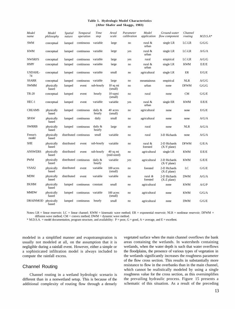
Table 1. Hydrologic Model Characteristics (After Shafer and Skaggs, 1983)

Model name

Model philosophy

Spatial nature

Temporal operation

Time step

Areal scale

Parameter calibration

Model application

Ground-water flow component

Channel routing M.D.S.A*

SWM conceptual lumped continuous variable large no rural & urban

single LR LC-LR G/G/G

KWM conceptual lumped continuous variable large yes rural & urban

single LR LC-LR A/G/A

NWSRFS conceptual lumped continuous variable large yes rural empirical LC-LR A/G/G HSPF conceptual lumped continuous variable large no rural &

urban single LR KWM E/E/E

USDAHL-74

conceptual lumped continuous variable small no agricultural single LR ER E/G/E

SSARR conceptual lumped continuous variable large no mountainous empirical NLR A/G/G SWMM physically

based lumped event sub-hourly 10 sq mi

(small) no urban none DFWM G/G/G

TR-20 conceptual lumped event hourly 10 sqmi (small)

no rural none CM G/G/E

HEC-1 conceptual lumped event variable variable yes rural & urban

single ER KWM E/E/E

CREAMS physically based

lumped continuous daily & hourly

40 acres (small)

no agricultural none none E/G/E

SPAW physically based

lumped continuous daily small no agricultural none none A/G/A

SWRRB physically based

lumped continuous daily & hourly

large no rural none NLR A/G/A

Freeze's model

physically based

distributed continuous small variable no rural 3-D Richards none A/G/A

SHE physically based

distributed event sub-hourly variable no rural & forested

2-D Richards (X-Y plane)

DFWM G/E/A

ANSWERS physically based

distributed event sub-hourly 40 sq mi (mid-sized)

no agricultural single LR KWM E/E/E

PWM physically based

distributed continuous daily & hourly

variable yes agricultural 2-D Richards (X-Y plane)

KWM G/E/E

VSAS2 physically based

distributed event variable 100 acres (small)

no forested 2-D Richards (X-Z plane)

LC G/G/E

MDM physically based

distributed event variable variable no rural & forested

2-D Richards (X-Z plane)

DWM A/G/A

ISUHM physically based

lumped continuous constant small no agricultural none KWM A/G/P

MMDW physically based

lumped continuous variable 100 acres (small)

no agricultural none KWM G/G/A

DRAINMOD physically based

lumped continuous hourly small no agricultural none DWM G/G/E

Notes: LR = linear reservoir; LC = linear channel; KWM = kinematic wave method; ER = exponential reservoir; NLR = nonlinear reservoir; DFWM = diffusion wave method; CM = convex method; DWM = dynamic wave method.

* M.D.S.A. = model documentation, program structure, and availability: P = poor, G = good, A = average, and E = excellent.

modeled in a simplified manner and evapotranspiration is usually not modeled at all, on the assumption that it is negligible during a rainfall event. However, either a simple or a sophisticated infiltration model is always included to compute the rainfall excess.

Channel Routing Channel routing in a wetland hydrologic scenario is

different than in a nonwetland setup. This is because of the additional complexity of routing flow through a densely

vegetated surface when the main channel overflows the bank areas containing the wetlands. In watersheds containing wetlands, when the water depth is such that water overflows the floodplains, the presence of various types of vegetation in the wetlands significantly increases the roughness parameter of the flow cross section. This results in substantially more resistance to flow in the overbanks than in the main channel, which cannot be realistically modeled by using a single roughness value for the cross section, as this oversimplifies the prevailing hydraulic process. Figure 15 presents a schematic of this situation. As a result of the preceding

13

observation, it was concluded that watershed areas containing wetlands require a flexible and rigorous channel-routing component to enable a more realistic route through the wetlands.

Channel routing can be defined as a mathematical technique to simulate the changing characteristics (magnitude, speed, and shape) of a water wave as it travels through canals, rivers, and estuaries (Fread, 1985). Channel routing can be accomplished at different levels of complexity. Basically, three general methodologies are cited in the literature. The first is empirical modeling, in which inflow is routed to the outlet by using a routing coefficient. These routing models are based on observations and analysis of historical streamflow data. As a result, their use is restricted to situations where the necessary inflow and outflow records for a channel reach are available. One of the most popular empirical routing models is known as Tatum's Successive Average Lag Method (U.S. Army Corps of Engineers, 1960), which may be expressed by the following relation:

where n is the number of subreaches obtained by dividing the travel time of the wave by the reach length, It+1 and Qt+1 are the inflow and the outflow at the end of the time interval, respectively, It,..., It-n+1 are the inflows at the preceding time steps, and CI,..., Cn+1 are the routing coefficients.

In the second methodology of channel routing, known as hydrologic routing, the continuity equation is coupled with a

Figure 15. Conceptual representation of channel flow in wetlands

storage versus inflow and/or outflow relationship. Perhaps the most well known and widely used of these is the Muskingum method (McCarthy, 1938), where storage is related to inflow and outflow through two parameters, a storage constant and a weighting factor. The corresponding final outflow equation may be represented by:

In the above equations, It and It+1 are the inflows at the beginning and end of the time step; Qt and Qt+1 are outflows at the beginning and end of the time step; C1-C3 are routing coefficients; K is the storage constant; X is the weighting coefficient; and Δt is the computational time step.

The third type of channel-routing model is based on the conservation of mass and momentum equations known as the Saint-Venant (1871) equations. These equations may be expressed as follows:

Conservation of Mass:

where A is the cross-sectional area, V is the velocity, x is the longitudinal distance, t is the time, g is the gravitational acceleration, y is the flow depth, S0 is the channel bottom slope, and Sf is the friction slope.

Because of their physical basis, methods of channel routing based on the Saint-Venant equations are called hydraulic models. All the hydraulic models are based either on the complete Saint-Venant equations or on some approximations thereof. When the full Saint-Venant equations are used, the resulting channel-routing model is called the dynamic wave model. If the first two terms (i.e., the inertia terms) in the momentum equation are neglected, the corresponding model is a diffusion wave model. When the momentum equation is expressed so that discharge is a single-valued function of depth, the corresponding model is a kinematic wave model. The implication is that the momentum of unsteady flow can be assumed to approximate that of steady uniform flow and may be expressed by the Chezy or Manning formula.

The different watershed models, listed in table 1 and reviewed previously, incorporate a variety of channel-routing

14

algorithms, which fall into one of the three categories defined in the preceding paragraphs. Table 2 provides a list of selected watershed models and their channel-routing capabilities. These models were chosen from those listed in table 1 on the basis of their channel-routing capabilities. Only hydraulic routing models, i.e., those based on the Saint-Venant equations or their approximations, were considered.

In addition, evaluations were made of three surface profile programs: WSPCP (Bureau of Reclamation, 1967), WSP2 (Soil Conservation Service, 1976), and HEC-2 (U.S. Army Corps of Engineers, 1972b). A dynamic wave channel-routing model, DWOPER (Fread, 1978), was also evaluated. Although the water-surface profile programs simulate steady-state flow and as such cannot be directly used for channel routing, they were nevertheless examined and included to illustrate how variations in channel geometry and roughness are incorporated into the modeling process. The dynamic wave model, DWOPER, is state-of-the-art in unsteady-state channel-routing modeling. This sophisticated model is based on the complete Saint-Venant equations.

Examination of the channel-routing algorithms of the different watershed models listed in table 2 reveals that most

of these models use algorithms based on physically based hydraulic equations, while resorting to considerable simplification in describing the geometry and hydraulic characteristics of the channel. Most of these algorithms assume a simple channel section, the most complicated being a trapezoidal section. Usually, no variation in roughness values along the cross section or the profile is taken into consideration. In contrast, all the surface profile models listed in table 2 take into account the variable roughness and geometric characteristics of the channel in the lateral and longitudinal directions. The DWOPER model is an advanced channel-routing model accom­modating many desirable characteristics for detailed channel-routing simulation. It incorporates features to take into account the variability in the geometry and the hydraulic characteristics along the channel cross sections and the longitudinal profile. It also allows variable time and space increments to be used in the computation. However, in this model, channel roughness variation along the lateral direction is taken into account either by relating the roughness parameter to depth or by providing con­veyance versus depth data for the cross sections.

Table 2. Model Channel-Routing Capabilities (After Eichert, 1970)

a b c d e f g h i j

Hydraulic assumptions Flow type

Cross section Roughness subdivisions

Roughness variation

with elevation Hydraulic

assumptions Flow type Shape Subdivisions Points Interpolation Extension Roughness

subdivisions

Roughness variation

with elevation P.DSA:

HSPF KWM/SPC Unsteady rect 1 no yes no E/E/E SWMM DFWM/SPC/SBC Unsteady trap/cir 1 no yes no G/G/G HEC-1 KWM/SPC Unsteady trap/cir 1 no yes no E/E/E SHE DFWM/SPC/SBC Unsteady rect 1 no yes no G/E/A ANSWERS KWM/SPC Unsteady rect 1 no yes no E/E/E PWM KWM/SPC Unsteady rect 1 no yes no G/E/E IHDM DWM/SPC/SBC Unsteady rect 1 no yes no A/G/A ISUHM KWM/SPC Unsteady trap 1 no yes no A/G/P MMDW KWM/SPC Unsteady trap 1 no yes no G/G/A DRAINMOD DWM/SPC/SBC Unsteady rect 1 no yes no G/G/E WSPCP SPC/SBC Steady any 9 100 no yes 9 yes A/A/G WSP2 SBC Steady any 3 48 no yes 3 no G/G/E HEC-2 SPC/SBC Steady any 100 100 yes yes 20 yes E/E/E DWOPER DWM/SPC/SBC Unsteady any 8 8 yes yes 1** yes E/E/E

Notes: KWM = kinematic wave method, SPC = supercritical flow, DFWM = diffusion wave method, SBC = subcritical flow; DWM = dynamic wave method * P.D S.A = program documentation, structure, and availability: P = poor , E = excellent, G = good; and A = average. ** Can incorporate this variation using conveyance versus depth data

15

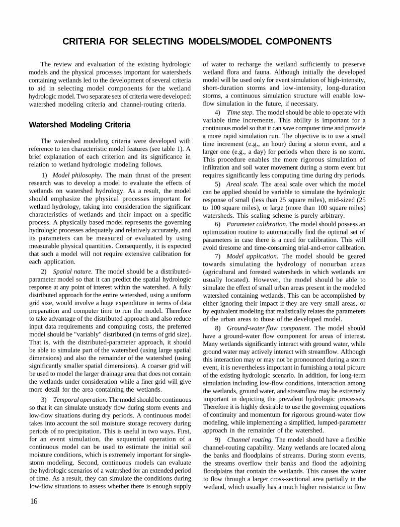
CRITERIA FOR SELECTING MODELS/MODEL COMPONENTS

The review and evaluation of the existing hydrologic models and the physical processes important for watersheds containing wetlands led to the development of several criteria to aid in selecting model components for the wetland hydrologic model. Two separate sets of criteria were developed: watershed modeling criteria and channel-routing criteria.

Watershed Modeling Criteria

The watershed modeling criteria were developed with reference to ten characteristic model features (see table 1). A brief explanation of each criterion and its significance in relation to wetland hydrologic modeling follows.

1) Model philosophy. The main thrust of the present research was to develop a model to evaluate the effects of wetlands on watershed hydrology. As a result, the model should emphasize the physical processes important for wetland hydrology, taking into consideration the significant characteristics of wetlands and their impact on a specific process. A physically based model represents the governing hydrologic processes adequately and relatively accurately, and its parameters can be measured or evaluated by using measurable physical quantities. Consequently, it is expected that such a model will not require extensive calibration for each application.

2) Spatial nature. The model should be a distributed-parameter model so that it can predict the spatial hydrologic response at any point of interest within the watershed. A fully distributed approach for the entire watershed, using a uniform grid size, would involve a huge expenditure in terms of data preparation and computer time to run the model. Therefore to take advantage of the distributed approach and also reduce input data requirements and computing costs, the preferred model should be "variably" distributed (in terms of grid size). That is, with the distributed-parameter approach, it should be able to simulate part of the watershed (using large spatial dimensions) and also the remainder of the watershed (using significantly smaller spatial dimensions). A coarser grid will be used to model the larger drainage area that does not contain the wetlands under consideration while a finer grid will give more detail for the area containing the wetlands.

3) Temporal operation. The model should be continuous so that it can simulate unsteady flow during storm events and low-flow situations during dry periods. A continuous model takes into account the soil moisture storage recovery during periods of no precipitation. This is useful in two ways. First, for an event simulation, the sequential operation of a continuous model can be used to estimate the initial soil moisture conditions, which is extremely important for single-storm modeling. Second, continuous models can evaluate the hydrologic scenarios of a watershed for an extended period of time. As a result, they can simulate the conditions during low-flow situations to assess whether there is enough supply

of water to recharge the wetland sufficiently to preserve wetland flora and fauna. Although initially the developed model will be used only for event simulation of high-intensity, short-duration storms and low-intensity, long-duration storms, a continuous simulation structure will enable low-flow simulation in the future, if necessary.

4) Time step. The model should be able to operate with variable time increments. This ability is important for a continuous model so that it can save computer time and provide a more rapid simulation run. The objective is to use a small time increment (e.g., an hour) during a storm event, and a larger one (e.g., a day) for periods when there is no storm. This procedure enables the more rigorous simulation of infiltration and soil water movement during a storm event but requires significantly less computing time during dry periods.

5) Areal scale. The areal scale over which the model can be applied should be variable to simulate the hydrologic response of small (less than 25 square miles), mid-sized (25 to 100 square miles), or large (more than 100 square miles) watersheds. This scaling scheme is purely arbitrary.

6) Parameter calibration. The model should possess an optimization routine to automatically find the optimal set of parameters in case there is a need for calibration. This will avoid tiresome and time-consuming trial-and-error calibration.

7) Model application. The model should be geared towards simulating the hydrology of nonurban areas (agricultural and forested watersheds in which wetlands are usually located). However, the model should be able to simulate the effect of small urban areas present in the modeled watershed containing wetlands. This can be accomplished by either ignoring their impact if they are very small areas, or by equivalent modeling that realistically relates the parameters of the urban areas to those of the developed model.

8) Ground-water flow component. The model should have a ground-water flow component for areas of interest. Many wetlands significantly interact with ground water, while ground water may actively interact with streamflow. Although this interaction may or may not be pronounced during a storm event, it is nevertheless important in furnishing a total picture of the existing hydrologic scenario. In addition, for long-term simulation including low-flow conditions, interaction among the wetlands, ground water, and streamflow may be extremely important in depicting the prevalent hydrologic processes. Therefore it is highly desirable to use the governing equations of continuity and momentum for rigorous ground-water flow modeling, while implementing a simplified, lumped-parameter approach in the remainder of the watershed.

9) Channel routing. The model should have a flexible channel-routing capability. Many wetlands are located along the banks and floodplains of streams. During storm events, the streams overflow their banks and flood the adjoining floodplains that contain the wetlands. This causes the water to flow through a larger cross-sectional area partially in the wetland, which usually has a much higher resistance to flow

16

than the main channel. Therefore a channel-routing algorithm is needed to realistically model these situations.

10) Model documentation, structure, and availability. The model should be well documented, have a modular program structure, and be available for immediate use. The documentation should clearly explain the model philosophy, subprocess modeling, and program structure. This will enable us not only to understand and use the model with relative ease, but also to modify, improve, or replace an individual algorithm, if necessary. The model should possess a modular programming structure with which to program the data input unit, results output unit, and the different subprocesses. The modular structure facilitates modification or change of isolated parts of the program without affecting the structure of the whole program. The program listing of the model should be easily available in a tape or diskette for a nominal price. This will ensure that the model can be obtained quickly and the work can be started without much delay.

Channel-Routing Criteria Because of the importance of the channel-routing

technique in the overall capability of the hydrologic model, channel-routing criteria have also been developed with reference to a number of characteristic features, similar to watershed modeling criteria. These criteria and their importance for detailed channel routing in a wetland hydrologic scenario are discussed below.

1) Flow type. What is the type of flow to be modeled: subcritical, supercritical, or both; uniform or nonuniform; steady or unsteady? Ideally, the proposed channel-routing algorithm should be able to model unsteady, nonuniform flow, both subcritical and supercritical.

2) Shape. What simplifying assumptions are made regarding the channel cross sections? Are these assumed to be rectangular, trapezoidal, or circular, or can the model handle any shape?

3) Subdivisions. To take into account the variability of velocity distribution along the transverse direction, it is necessary to use as many cross-sectional subdivisions as possible on the basis of the available data. These subdivisions can also be used to consider the geometric variability and variation in the Manning roughness coefficient in the transverse direction.

4) Description. If the model can incorporate cross sections of any shape, what is the maximum number of points used to delineate such a section? In other words, with how much precision can the cross sections be defined?

5) Interpolation. This is extremely important for incorporating variable Ax when implementing the numerical algorithm of the channel-routing model. Without this capability, it will not be possible to accommodate different Ax values over the channel reach. This means not only that a single Ax value has to be used for the entire reach, but also that the data provided to the model have to be available at these constant intervals or have to be interpolated manually or by using a preprocessor program from existing data at variable Ax values.

6) Vertical extension. When a channel-routing program is executed, computed flow depths may exceed the maximum depth listed in the cross-section and depth data provided as program input. In such a situation, it is necessary to have an option to extend the cross section vertically by using a suitable extrapolation technique.

7) Roughness subdivisions. The channel-routing algorithm should have the capability to use varying roughness coefficients for different transverse cross-sectional subdivisions. This ensures consideration of the changes in roughness values from the main channel to the overbanks.

8) Roughness variation with elevation. Because roughness coefficients may also vary with depth of water, it is very useful if the channel-routing method has such a provision. Another use of this provision is to take into account the variation of roughness along cross-sectional subdivisions in case that is not explicitly provided in the channel cross-section data. Based on available information, a relationship may be developed for roughness and depth of water. The roughness values should be the weighted average values as the water overflows from the main channel into the overbanks. This procedure implicitly lumps the variation of roughness along the cross section with depth. The cross-sectional information in this case only provides more adequate representation of the geometry of the channel sections for computing the given section's wetted perimeter, hydraulic radius, and so forth.

9) Program documentation, structure, and availability. The last criterion in selecting a channel-routing algorithm is extremely important from a practical point of view. Three significant points must be taken into consideration in this context. The channel-routing model has to be well documented so that it can be easily understood. The algorithm should possess a modular programming structure so that it is clear, coherent, and compact. The listing of the channel-routing algorithm should be available in a tape or diskette at a nominal price so that it can be quickly procured and incorporated into the proposed wetland watershed model.

17

MODEL FORMULATION

After a review of the capabilities of the watershed models listed in table 1 and the channel-routing models listed in table 2, it was concluded that none of the models have all the attributes needed to simulate wetland hydrology as envisioned in this project. Therefore it was necessary to select desirable components from the existing models and combine them with new components to develop the wetland hydrology model.

The procedure for developing the proposed wetland hydrology model was to select a base model as a starting point and then to improve certain components, incorporating additional components from other models or new ones as necessary. The procedure has two interrelated steps: selec­tion of watershed components and selection of the channel-routing component.

Selection of Watershed Model and Its Components

The base model should provide the infrastructure for building the proposed wetland hydrology model. Its components should simulate interception, evapotranspiration, infiltration, drainage, overland flow, and ground-water flow.

Choice of the Base Model

Since one of the primary goals of this research was to develop a model that can simulate the hydrologic response of a watershed containing wetlands at different watershed locations, the model's philosophy and spatial nature are extremely important. A physically based model is necessary to accurately depict the physical processes governing the wetland behavior without requiring extensive parameter calibration. A distributed-parameter model permits evaluation of the effect of any wetland anywhere in the watershed with proper consideration of its spatial location.

From the foregoing observations, it is concluded that the basic framework of the model should be that of a distributed model, and that its major processes should be formulated by using physically based equations. As discussed previously, very few distributed models are cited in the literature. Among the models developed in North America, the following were con­sidered as possible choices for the base model: the ANSWERS model, VSAS2, and Freeze's model. Two models developed in Europe were also examined: the SHE model and IHDM.

Both Freeze's model and the SHE model were not chosen as the base model because of the huge input data requirement and the computing costs necessary to run these models. The IHDM, on the other hand, was assessed to be inappropriate for the proposed research since it employs a simplified geometric description of the watershed. Although all three models possess modular programming structures, it may be very dif­ficult to obtain program listings and documentation for them.

ANSWERS, one of the remaining two potential models, couples two-dimensional overland flow and one-dimensional channel flow with an infiltration equation. It models ground­water flow in a simple manner by using a storage function. On the other hand, VSAS2, couples one-dimensional overland flow and one-dimensional channel flow with two-dimensional subsurface flow. One of the dimensions in the subsurface flow equation used in VSAS2 represents vertical infiltration, while the other dimension simulates downslope subsurface flow. Overland flow routing is not done, and channel routing is performed simply by using a lag term. Both ANSWERS and VSAS2 are well documented: program listings and user manuals for these models can easily be obtained. These two models were developed by using a modular structure.

The evaluation of the existing models indicated that, for the present project, both the ANSWERS model and VSAS2 possess the general structure and other features required for the base model to accomplish the stated goal of the research. Upon further evaluation, it was concluded that the ANSWERS model offers the best framework for developing a wetland hydrologic model meeting the significant criteria. ANSWERS is a tested, well-documented, readily available distributed-parameter model. However, some modifications will be required to develop the model envisaged in this project.

The first modification pertains to the model's distributed-parameter structure. The ANSWERS model uses a fixed grid size. To model wetland hydrology rigorously while keeping computing costs reasonable, the proposed model should be "variably" distributed so that the watershed can be simulated with variable grid sizes. The algorithm therefore has to be changed accordingly.

The rest of the modifications involve incorporating additional hydrologic model components. These component modifications are discussed in the following section.

Selection of Hydrologic Process Models

The necessary hydrologic components for the proposed wetland hydrology model were selected on the basis of existing model capabilities as discussed previously and summarized in table 1. These components include algorithms for interception, evapotranspiration, infiltration, drainage, overland flow, ground-water flow, and channel routing. The channel-routing component is discussed separately. A discussion of the other components follows.

Interception. The interception component of the ANSWERS model will be retained as is since it was based on the canopy storage accounting procedure used with success in the ANSWERS model.

Evapotranspiration. The ANSWERS model does not have a component for evapotranspiration. Therefore a decision was made to add an evapotranspiration component based on the Penman equation as in the MMDW.

18

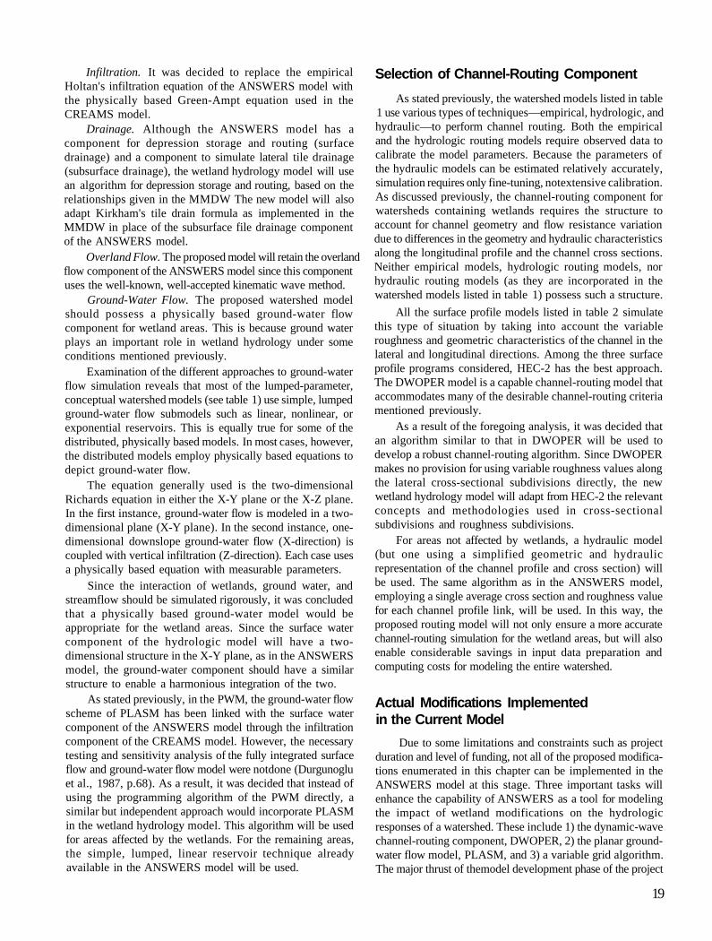
Infiltration. It was decided to replace the empirical Holtan's infiltration equation of the ANSWERS model with the physically based Green-Ampt equation used in the CREAMS model.

Drainage. Although the ANSWERS model has a component for depression storage and routing (surface drainage) and a component to simulate lateral tile drainage (subsurface drainage), the wetland hydrology model will use an algorithm for depression storage and routing, based on the relationships given in the MMDW The new model will also adapt Kirkham's tile drain formula as implemented in the MMDW in place of the subsurface file drainage component of the ANSWERS model.

Overland Flow. The proposed model will retain the overland flow component of the ANSWERS model since this component uses the well-known, well-accepted kinematic wave method.

Ground-Water Flow. The proposed watershed model should possess a physically based ground-water flow component for wetland areas. This is because ground water plays an important role in wetland hydrology under some conditions mentioned previously.

Examination of the different approaches to ground-water flow simulation reveals that most of the lumped-parameter, conceptual watershed models (see table 1) use simple, lumped ground-water flow submodels such as linear, nonlinear, or exponential reservoirs. This is equally true for some of the distributed, physically based models. In most cases, however, the distributed models employ physically based equations to depict ground-water flow.

The equation generally used is the two-dimensional Richards equation in either the X-Y plane or the X-Z plane. In the first instance, ground-water flow is modeled in a two-dimensional plane (X-Y plane). In the second instance, one-dimensional downslope ground-water flow (X-direction) is coupled with vertical infiltration (Z-direction). Each case uses a physically based equation with measurable parameters.

Since the interaction of wetlands, ground water, and streamflow should be simulated rigorously, it was concluded that a physically based ground-water model would be appropriate for the wetland areas. Since the surface water component of the hydrologic model will have a two-dimensional structure in the X-Y plane, as in the ANSWERS model, the ground-water component should have a similar structure to enable a harmonious integration of the two.

As stated previously, in the PWM, the ground-water flow scheme of PLASM has been linked with the surface water component of the ANSWERS model through the infiltration component of the CREAMS model. However, the necessary testing and sensitivity analysis of the fully integrated surface flow and ground-water flow model were notdone (Durgunoglu et al., 1987, p.68). As a result, it was decided that instead of using the programming algorithm of the PWM directly, a similar but independent approach would incorporate PLASM in the wetland hydrology model. This algorithm will be used for areas affected by the wetlands. For the remaining areas, the simple, lumped, linear reservoir technique already available in the ANSWERS model will be used.

Selection of Channel-Routing Component As stated previously, the watershed models listed in table

1 use various types of techniques—empirical, hydrologic, and hydraulic—to perform channel routing. Both the empirical and the hydrologic routing models require observed data to calibrate the model parameters. Because the parameters of the hydraulic models can be estimated relatively accurately, simulation requires only fine-tuning, notextensive calibration. As discussed previously, the channel-routing component for watersheds containing wetlands requires the structure to account for channel geometry and flow resistance variation due to differences in the geometry and hydraulic characteristics along the longitudinal profile and the channel cross sections. Neither empirical models, hydrologic routing models, nor hydraulic routing models (as they are incorporated in the watershed models listed in table 1) possess such a structure.

All the surface profile models listed in table 2 simulate this type of situation by taking into account the variable roughness and geometric characteristics of the channel in the lateral and longitudinal directions. Among the three surface profile programs considered, HEC-2 has the best approach. The DWOPER model is a capable channel-routing model that accommodates many of the desirable channel-routing criteria mentioned previously.

As a result of the foregoing analysis, it was decided that an algorithm similar to that in DWOPER will be used to develop a robust channel-routing algorithm. Since DWOPER makes no provision for using variable roughness values along the lateral cross-sectional subdivisions directly, the new wetland hydrology model will adapt from HEC-2 the relevant concepts and methodologies used in cross-sectional subdivisions and roughness subdivisions.

For areas not affected by wetlands, a hydraulic model (but one using a simplified geometric and hydraulic representation of the channel profile and cross section) will be used. The same algorithm as in the ANSWERS model, employing a single average cross section and roughness value for each channel profile link, will be used. In this way, the proposed routing model will not only ensure a more accurate channel-routing simulation for the wetland areas, but will also enable considerable savings in input data preparation and computing costs for modeling the entire watershed.

Actual Modifications Implemented in the Current Model

Due to some limitations and constraints such as project duration and level of funding, not all of the proposed modifica­tions enumerated in this chapter can be implemented in the ANSWERS model at this stage. Three important tasks will enhance the capability of ANSWERS as a tool for modeling the impact of wetland modifications on the hydrologic responses of a watershed. These include 1) the dynamic-wave channel-routing component, DWOPER, 2) the planar ground­water flow model, PLASM, and 3) a variable grid algorithm. The major thrust of themodel development phase of the project

19

has been directed towards accomplishing these three tasks. The dynamic routing component and the variable grid algorithm were successfully implemented in ANSWERS. Due to some unresolved programming errors, however, we were unable to incorporate the ground-water flow algorithm into the new model before the project duration expired. In a future

study we hope to address the physically based ground-water flow algorithm and the other proposed modifications, including the use of Penman's evaporation equation and the Kirkham file-drain formula. The next chapter describes the processes included in the watershed and channel-routing components of the current version of the wetland hydrology model.

20

MODEL DEVELOPMENT

A detailed description of the wetland hydrology model, comprising the watershed model and the dynamic wave channel-routing components, is given in this section. The hydrologic and hydraulic processes that constitute the bases of these component models are also discussed.

Watershed Model Components The core program for the watershed model components

was based on a distributed-parameter model, ANSWERS, which was developed by Beasley (1977) for application to small agricultural watersheds. Development of the mathe­matical model was based on the assumption that the spatial and temporal parameters of a watershed can be represented as discrete variables. The watershed was subdivided into square elements as shown previously in figure 8. The element size was chosen to ensure relatively uniform spatial variability of significant watershed parameters such as slope, vegetation, infiltration rate, land use, and so forth. However, these parameters may change from element to element. The elements interact through the continuity of surface flow, tile drain flow, and baseflows across element boundaries. The continuity of flow implies that the outflow from an element becomes the inflow into adjacent downslope elements. The surface flow component of the watershed model comprises overland flow and channel flow.

The channel-routing component in the watershed model is applied to route tributary flow. A dynamic channel-routing component, which is described later, is applied where the variation of cross-sectional profile and channel flow characteristics significantly influences the flow.

The watershed model comprises the basic hydrologic components, which include interception, depression storage, infiltration, subsurface drainage, tile drainage, baseflow, overland flow, and channel flow. These hydrologic processes are described in the following sections.

Interception

During a rainstorm, interception is that portion of the rain that wets and adheres to vegetation and canopy surfaces as a thin film and that also fills depressions on the trunks of plants and trees. This water is eventually lost to the atmosphere through evaporation. Interception is a function of storm char­acteristics, plant species type, vegetation density, and season of the year. Water losses due to interception will increase with increasing density and surface area of the vegetal cover. The surface characteristics of the canopy determine the thickness of the water film that will adhere to the exposed surface.

A large portion of the interception losses occur at the beginning of the rainstorm, and the interception rate thereafter decreases rapidly to zero. The distribution of the interception losses during an individual storm is generally not known. The approach used in the watershed model component involves

the specification of a maximum potential interception (PIT), which is defined as the available leaf moisture storage. Typical PIT values for different crops are shown in table 3. At each time step, the PIT value is reduced by the product of the rainfall rate and the percentage of the elemental land area covered by vegetation and other types of cover. When the maximum interception rate is satisfied, the gauge rainfall rate becomes the net rainfall rate for the remainder of the simulation period.

Table 3. Potential Interception Values (After Beasley and Huggins, 1982)

Potential Crop interception

(in inches) Oats 0.020-0.039 Corn 0.012-0.051 Grass 0.020-0.039 Pasture and meadow 0.012-0.020 Wheat, rye, and barley 0.012-0.039 Beans, potatoes, and cabbage 0.020-0.059 Woods 0.039-0.098

Depression Storage

The portion of the rainfall that is not intercepted reaches the ground surface and will either infiltrate or fill up surface depressions or become runoff. The filling of surface depressions starts as soon as the rainfall rate exceeds the infiltration rate. As individual surface depressions are inundated, the excess rainwater becomes runoff. This runoff will fill other depressions or flow directly into adjacent streamchannels. When the rainfall ends and the runoff has receded, a portion of the water in the depressions will evaporate and some will infiltrate the soil, becoming part of the interflow and may eventually reemerge to contribute to surface runoff. Depending on the infiltration characteristics of the soil, some of the depressions may be ponded for several hours or days.

Natural processes and land-use practices continuously alter the shapes and sizes of natural depressions. The volume of water in depression storage at any given time during a storm can be expressed as a function of the accumulated rainfall excess. Huggins and Monke (1966) used the topographical relief profile similar to figure 16 to formulate a storage-depth

Figure 16. Ground surface topographical profile used to derive surface storage relations

21

relation for an elemental area. The derivation is based on the assumption that the depressions are filled before runoff starts and that evaporation before and after the rainstorm is negligible. The water level is assumed to be uniform over the area, and the depth, h, is taken as zero at the lowest point of the depressions. By analyzing several microdepressional profiles produced by different tillage practices, Huggins and Monke obtained a surface storage-depth relation expressed as:

where: Su = volume of stored water Sv=hu*(Δx)2 h - physical depth of stored water above the lowest

elevation in the depressions hu= height of the highest point above the lowest elevation

or datum Δx = length of the side of a square element a,b = constants

The derivative of Su with respect to h is equal to the surface area of the water within the depressions. By differentiating Su with respect to h using equation (8) and substituting for Sv, we obtain:

If the ratio of the surface area of the water inside the depressions to the elemental area, (Ax)2, is represented by FWA, then:

When h = h , the depressions are completely filled with water and the water surface area will be equal to the elemental area, i.e., FWA - 1. Hence under this condition, equation (1) yields

ab =1 or b = 1/a (11)

Equation (10) is then reduced to:

If h is eliminated from (12), using (8), we obtain:

Since h is a distributed variable, a retention depth cannot be computed for each element. However, we can define an average retention depth, d, as the volume of stored water divided by the area of the element, i.e.,

By taking a as the roughness coefficient, rc, we can now express FWA as:

Since Su, the rainfall volume in excess of interception storage, is known at each time step, d can be evaluated and used to compute FWA from equation (15). Typical values of rc and hu for different land-use and cover types are given in table 4. rc varies from 0.30 to 0.75. The higher the value of rc, the more sinuous the soil surface.

Table 4. Surface Storage and Roughness Parameters (Adapted from Beasley and Huggins, 1982)

hu

Land use or cover rc (inches) n0 Grass or pasture Poor cover 0.40 1.0 0.080 Average cover 0.45 1.5 0.100 Good cover 0.50 1.5 0.120

Forests or wooded area Light woods 0.55 2.5 0.150 Heavy woods 0.60 3.0 0.200

Turn plowed ground Smooth 0.30 1.5 0.035 Rough 0.75 6.0 0.350

Chisel plowed ground Smooth 0.40 2.5 0.050 Rough 0.65 4.0 0.250

FWA represents the saturated infiltration zone in an element where the ground surface is inundated or where the rainfall rate exceeds the infiltration capacity. The unsaturated infiltration zone in the element is (1-FWA). If the maximum infiltration capacity is denoted by Fmax and the rainfall rate by R, the infiltration capacity, FILT, within an element when the rainfall rate is less than the maximum infiltration capacity (i.e., R < Fmax) is given by the following expression:

However, when the rainfall rate exceeds the maximum infiltration capacity (i.e ., R>Fmax), then:

Infiltration

Infiltration plays an important role in the timing and distribution of runoff in a watershed. It is defined as the flow of water through the ground surface into the underlying strata. It is distinguished from percolation, which is the movement of water in the soil strata. The infiltration rate is influenced

22

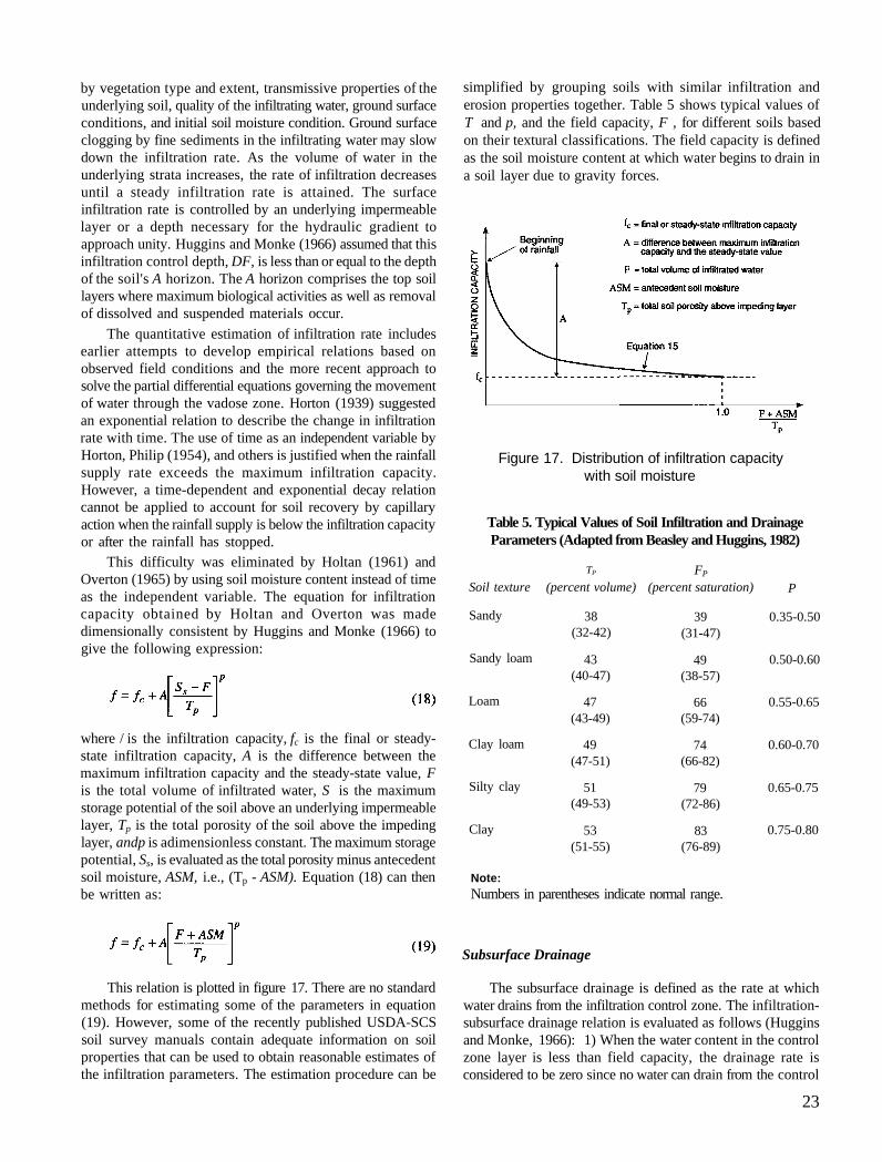
by vegetation type and extent, transmissive properties of the underlying soil, quality of the infiltrating water, ground surface conditions, and initial soil moisture condition. Ground surface clogging by fine sediments in the infiltrating water may slow down the infiltration rate. As the volume of water in the underlying strata increases, the rate of infiltration decreases until a steady infiltration rate is attained. The surface infiltration rate is controlled by an underlying impermeable layer or a depth necessary for the hydraulic gradient to approach unity. Huggins and Monke (1966) assumed that this infiltration control depth, DF, is less than or equal to the depth of the soil's A horizon. The A horizon comprises the top soil layers where maximum biological activities as well as removal of dissolved and suspended materials occur.

The quantitative estimation of infiltration rate includes earlier attempts to develop empirical relations based on observed field conditions and the more recent approach to solve the partial differential equations governing the movement of water through the vadose zone. Horton (1939) suggested an exponential relation to describe the change in infiltration rate with time. The use of time as an independent variable by Horton, Philip (1954), and others is justified when the rainfall supply rate exceeds the maximum infiltration capacity. However, a time-dependent and exponential decay relation cannot be applied to account for soil recovery by capillary action when the rainfall supply is below the infiltration capacity or after the rainfall has stopped.

This difficulty was eliminated by Holtan (1961) and Overton (1965) by using soil moisture content instead of time as the independent variable. The equation for infiltration capacity obtained by Holtan and Overton was made dimensionally consistent by Huggins and Monke (1966) to give the following expression:

where / is the infiltration capacity, fc is the final or steady-state infiltration capacity, A is the difference between the maximum infiltration capacity and the steady-state value, F is the total volume of infiltrated water, S is the maximum storage potential of the soil above an underlying impermeable layer, Tp is the total porosity of the soil above the impeding layer, andp is adimensionless constant. The maximum storage potential, Ss, is evaluated as the total porosity minus antecedent soil moisture, ASM, i.e., (Tp - ASM). Equation (18) can then be written as:

This relation is plotted in figure 17. There are no standard methods for estimating some of the parameters in equation (19). However, some of the recently published USDA-SCS soil survey manuals contain adequate information on soil properties that can be used to obtain reasonable estimates of the infiltration parameters. The estimation procedure can be

simplified by grouping soils with similar infiltration and erosion properties together. Table 5 shows typical values of T and p, and the field capacity, F , for different soils based on their textural classifications. The field capacity is defined as the soil moisture content at which water begins to drain in a soil layer due to gravity forces.

Figure 17. Distribution of infiltration capacity with soil moisture

Table 5. Typical Values of Soil Infiltration and Drainage Parameters (Adapted from Beasley and Huggins, 1982)

TP FP

Soil texture (percent volume) (percent saturation) P

Sandy 38 (32-42)

39 (31-47)

0.35-0.50

Sandy loam 43 (40-47)

49 (38-57)

0.50-0.60

Loam 47 (43-49)

66 (59-74)

0.55-0.65

Clay loam 49 (47-51)

74 (66-82)

0.60-0.70

Silty clay 51 (49-53)

79 (72-86)

0.65-0.75

Clay 53 (51-55)

83 (76-89)

0.75-0.80

Note: Numbers in parentheses indicate normal range.

Subsurface Drainage

The subsurface drainage is defined as the rate at which water drains from the infiltration control zone. The infiltration-subsurface drainage relation is evaluated as follows (Huggins and Monke, 1966): 1) When the water content in the control zone layer is less than field capacity, the drainage rate is considered to be zero since no water can drain from the control

23

zone. 2) The soil is assumed to be completely saturated when the rate of infiltration becomes steady. The subsurface drainage rate is then equal to the steady-state infiltration rate so that continuity of flow through an imaginary control volume drawn around the control zone layer is satisfied. 3) If the water content is between field capacity and saturation, the subsurface drainage rate is obtained from the following expression:

where Gv - maximum volume of gravitational water, i.e., (TP - FP). The drainage rate becomes steady as (Ss - F) approaches zero. The drainage water leaving the control zone contributes to tile drainflow and ground-water storage and may become part of interflow and eventually emerge as runoff into the channel segments.

Tile Drainage

The subsurface drainage water leaving the control zone contributes to tile drainage in all overland flow elements containing tile drains. A drainage capacity, DC, defined as the maximum rate of flow in each tile drain, is assigned to each tiled element. The drainage rate in excess of the drainage capacity for tiled elements is added to the ground-water reservoir.

The total tile drainage rate through an element is the sum of the accumulated tile drainage inflow rate from upslope overland-flow elements and the element's subsurface drainage rate from the infiltration control zone up to the limit of the assigned tile drainage capacity. The accumulated tile drainage rate is proportioned to downslope elements, using the same routing procedure as in the overland flow. For channel segments, the accumulated tile drainage rates from upstream elements are added as inflow. For untiled elements, tile drainage flow is equal to zero.

Baseflow

The subsurface drainage water, which leaves the infiltration control zone in untiled elements, and the subsurface flow, which is in excess of the tile drainage capacity in tiled elements, are added to a common ground-water reservoir. At each time step, the channel baseflow is simulated by releasing a fraction of the ground-water storage volume into the channel segments at an equal rate. The channel baseflow in each channel segment is computed as the average baseflow released during the routing interval, Ix, in a time step as:

where Gf is the ground-water release fraction, Gws is the ground­water storage rate, Nc is the number of channel segments, and ß is a constant. The ground-water storage is depleted by the sum of channel baseflow released into all channel segments at the end of each time step. A schematic representation of the subsurface drainage components is shown in Figure 18.

Figure 18. Schematic diagram of subsurface drainage

Overland Flow

As the storage volume in each microdepression and macrodepression is satisfied, the excess rainfall becomes overland-flow runoff. The overland flow is routed downstream based on the assumption of the existence of continuity of flow. This assumption implies that a functional relation exists between water depth and surface runoff at every point within the watershed elements. This variation of depth with surface runoff depends on the slope of the elements, the characteristics of the micro- and macrorelief, and the turbulence characteristics of the flow. A typical depth-discharge relation is shown in figure 19, which indicates that once the surface depressional storage is satisfied at d, which is theoretically equal to hu when surface runoff commences, the surface runoff will increase as the water depth increases. Since the effects of microscale relief are usually masked by macroscale characteristics, a quantitative description of overland flow is difficult. However, an average flow condition can be defined

Figure 19. Depth-runoff relations for overland flow 24

in each watershed element such that the average cross-sectional depth of flow, d, for overland flow is given by:

where: S = storage volume for overland flow depth, d Sr = maximum surface depressional storage volume prior

to initiation of runoff Since the runoff is defined by Q = V*A, where A is the cross-sectional area of flow, the average velocity of flow, V, can be evaluated using the Manning equation for steady turbulent flow in open channels. The Manning equation is expressed as:

m = 2/3 S0 = average overland element slope n = Manning's hydraulic roughness coefficient for

overland element C = 1.486 (English units) or 1.0 (metric units)

The runoff can then be expressed as:

The width of the overland-flow cross section is taken as the length of the sides of a square element. The overland runoff in each element is assumed to be in the direction of the steepest slope, a, measured counterclockwise from the positive x axis as shown in figure 20(a). The steepest slope direction is used to proportion and route the flow from an element to adjacent row and column elements. The outflow from each overland-flow element is not allowed to flow into diagonal elements. The slope direction for a typical element is shown by the arrowed lines in figure 20(b). It is assumed that the horizontal component of flow, QH, across the element face AB in figure 20(b) is proportional to the area ABC (AH) and that the vertical flow component, Qv, across face AE is proportional to the area ACDE (Av). Therefore, the horizontal and vertical components of flow are expressed as:

In figure 20(a), the angle of inclination of the steepest slope direction to the vertical, 6, is calculated as:

where N is the quadrant number. Hence, the fraction of flow, fr, for 0 ≤θ≤45 is given by:

Tributary Channel Flow

The watershed model component uses dual elements for the channel segments by specifying pseudo-overland-flow elements for the corresponding channel segment elements. The routing of flow in tributary channels is based on the following assumptions: 1) The channel slope direction can be specified only along 0, 45, 90,...,315, and 360 degrees, i.e., in increments of 45 degrees. 2) No infiltration is allowed through the channel bed and banks. 3) Only rectangular channel cross section and uniform roughness parameters are permitted in each channel segment. The channel length is equal to the length of the sides of the pseudoelement if the flow direction is along the horizontal or vertical axis. Otherwise, the channel length is equal to the length of the diagonal of the element (i.e., Δx) if the slope direction is along any of the diagonals.

The flow in tributary channels is also described by the Manning equation that was used for overland flow routing except that, in this case, the top width of the channel cross section is used instead of the length of the sides of the element. One half of the overland element slope is used when the slope of the channel segment is not specified in the input. The Manning equation for open-channel flow is described by:

where B is the top width of the channel cross section, y is the water depth, nc is the Manning's channel roughness coefficient, and Sc is the channel-segment slope.

The total inflow into the tributary channel segments includes the flow from pseudo-overland-flow elements, tile drainflow, baseflow, and the inflow from upstream tributary channel segments. The total inflow is subsequently routed through the tributary channels to the junctions with the main channel.

Overland and Channel Flow Routing

The routing of overland and tributary channel flow is based on the continuity equation. The mass balance relation for inflow, outflow, and rate of accumulation of storage within

25

Figure 20. Horizontal and vertical components of discharge

each element is described by:

For a time interval, At, the continuity equation can be expressed in terms of average flow as:

where /, Q, and S represent the average inflow, outflow, and storage volume, respectively. The subscripts 1 and 2 refer to the beginning and end of the time interval. In equation (35), the initial inflow I1, outflow Q1 and storage S1, and the final inflow I2 are known. The only unknown variables are Q2 and S2 A second equation is therefore required to obtain the

solution for Q2 and S2. The additional equation is provided by equations (25) and (33), which express the outflow as a function of water depth. The storage volume for overland flow is expressed as:

and for channel flow as:

where K=l for vertical and horizontal flow and K= for diagonal flow. Using these expressions to eliminate from equation (25) and y from equation (33) yields the general relation for outflow as:

26

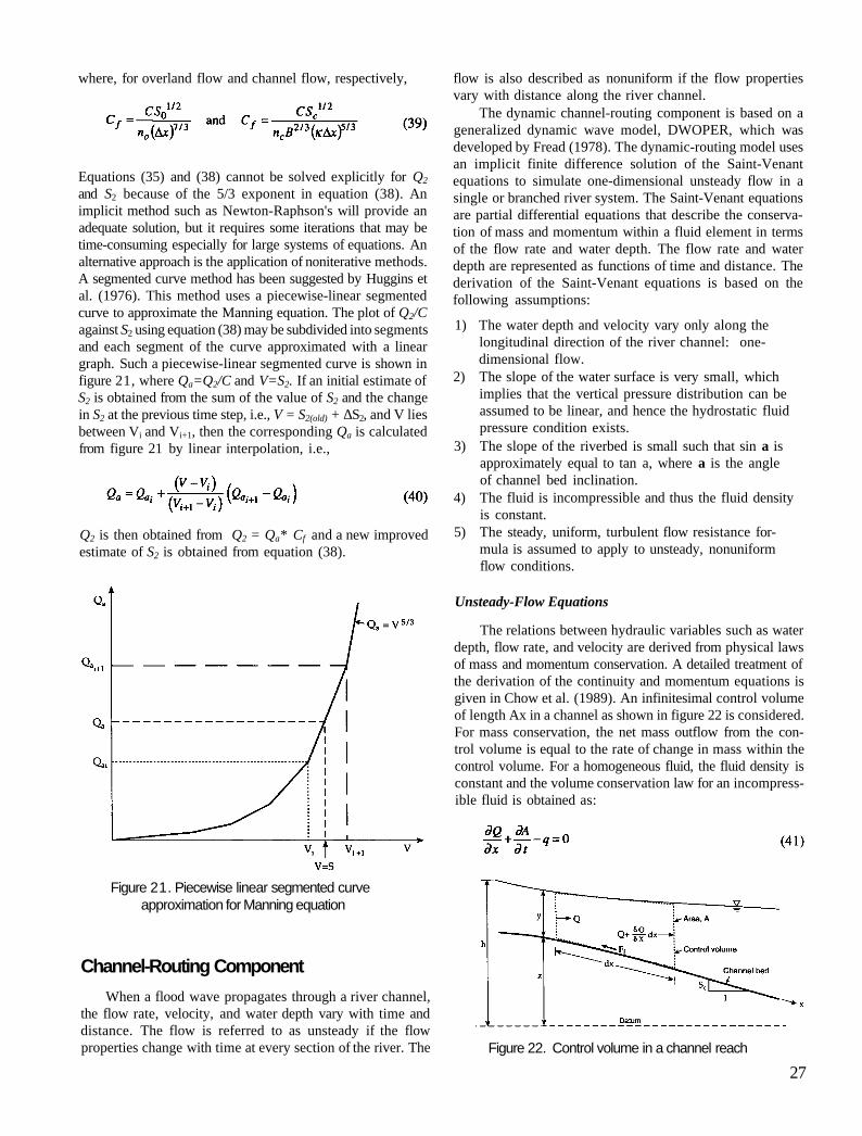
where, for overland flow and channel flow, respectively,

Equations (35) and (38) cannot be solved explicitly for Q2 and S2 because of the 5/3 exponent in equation (38). An implicit method such as Newton-Raphson's will provide an adequate solution, but it requires some iterations that may be time-consuming especially for large systems of equations. An alternative approach is the application of noniterative methods. A segmented curve method has been suggested by Huggins et al. (1976). This method uses a piecewise-linear segmented curve to approximate the Manning equation. The plot of Q2/C against S2 using equation (38) may be subdivided into segments and each segment of the curve approximated with a linear graph. Such a piecewise-linear segmented curve is shown in figure 21, where Qa=Q2/C and V=S2. If an initial estimate of S2 is obtained from the sum of the value of S2 and the change in S2 at the previous time step, i.e., V = S2(old) + ΔS2, and V lies between Vi and Vi+1, then the corresponding Qa is calculated from figure 21 by linear interpolation, i.e.,

Q2 is then obtained from Q2 = Qa* Cf and a new improved estimate of S2 is obtained from equation (38).

Figure 21. Piecewise linear segmented curve approximation for Manning equation

Channel-Routing Component When a flood wave propagates through a river channel,

the flow rate, velocity, and water depth vary with time and distance. The flow is referred to as unsteady if the flow properties change with time at every section of the river. The

flow is also described as nonuniform if the flow properties vary with distance along the river channel.

The dynamic channel-routing component is based on a generalized dynamic wave model, DWOPER, which was developed by Fread (1978). The dynamic-routing model uses an implicit finite difference solution of the Saint-Venant equations to simulate one-dimensional unsteady flow in a single or branched river system. The Saint-Venant equations are partial differential equations that describe the conserva­tion of mass and momentum within a fluid element in terms of the flow rate and water depth. The flow rate and water depth are represented as functions of time and distance. The derivation of the Saint-Venant equations is based on the following assumptions:

1) The water depth and velocity vary only along the longitudinal direction of the river channel: one-dimensional flow.

2) The slope of the water surface is very small, which implies that the vertical pressure distribution can be assumed to be linear, and hence the hydrostatic fluid pressure condition exists.

3) The slope of the riverbed is small such that sin a is approximately equal to tan a, where a is the angle of channel bed inclination.

4) The fluid is incompressible and thus the fluid density is constant.

5) The steady, uniform, turbulent flow resistance for­mula is assumed to apply to unsteady, nonuniform flow conditions.

Unsteady-Flow Equations

The relations between hydraulic variables such as water depth, flow rate, and velocity are derived from physical laws of mass and momentum conservation. A detailed treatment of the derivation of the continuity and momentum equations is given in Chow et al. (1989). An infinitesimal control volume of length Ax in a channel as shown in figure 22 is considered. For mass conservation, the net mass outflow from the con­trol volume is equal to the rate of change in mass within the control volume. For a homogeneous fluid, the fluid density is constant and the volume conservation law for an incompress­ible fluid is obtained as:

Figure 22. Control volume in a channel reach

27

where Q is the flow rate, A is the average cross-sectional area, q is the lateral inflow in units of flow rate per unit channel length, x is the distance along the longitudinal axis of the river channel, and t is the time. Equation (41) is called the continuity equation.

The momentum equation is obtained from Newton's second law of motion, which states that the sum of the forces acting on a fluid element is equal to the rate of change of momentum within the control volume. The four forces considered to be acting on the control volume are gravity, friction, drag due to eddies created by abrupt changes in the cross section, and pressure. For a constant density fluid, the momentum equation for open-channel flow is given by:

where Sf is the frictional slope, Se is the eddy loss slope, h is the water surface elevation, g is the gravity acceleration, and v is the velocity of the lateral inflow along the longitudinal axis of the channel.

The frictional slope and the eddy slope are defined as:

where R is the hydraulic radius and K is the expansion-contraction coefficient.

Finite Difference Solution

The solution of the partial differential equations, (41) and (42), are sought for variables Q and h at selected sections along the channel and at different discrete times. The solution domain can be represented on the x-t plane by a net of nodal positions with subscript j representing the time lines and subscript i, the x positions. An implicit finite difference scheme using a weighted four-point method (Amein and Fang, 1970; Liggett and Cunge, 1975) as shown in figure 23

Figure 23. The four-point scheme for finite difference discretization

can be applied to transform an arbitrary function / and its spatial and time derivatives to the following expressions:

where f'. denotes the value of / at node (i, j), i denotes the sequence number of the Ax reaches, j denotes the sequence number of the time lines, and 9 is a weighting factor that varies between 0.5 and 1. A value of 6 close to 0.5 gives a linearly stable and accurate solution. However, a weak or pseudoinstability sometimes develop when Bis used. Fread (1978) recommended that a value of 6 between 0.55 and 0.6 produces a more stable solution but with a slight loss of accuracy.

By using these finite difference approximations in equations (41) and (42), the finite difference forms of the continuity and momentum equations are obtained as:

28

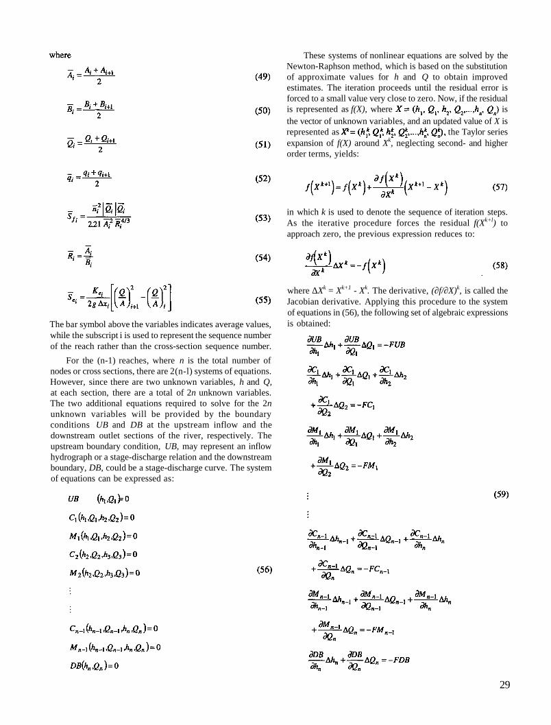
The bar symbol above the variables indicates average values, while the subscript i is used to represent the sequence number of the reach rather than the cross-section sequence number.

For the (n-1) reaches, where n is the total number of nodes or cross sections, there are 2(n-l) systems of equations. However, since there are two unknown variables, h and Q, at each section, there are a total of 2n unknown variables. The two additional equations required to solve for the 2n unknown variables will be provided by the boundary conditions UB and DB at the upstream inflow and the downstream outlet sections of the river, respectively. The upstream boundary condition, UB, may represent an inflow hydrograph or a stage-discharge relation and the downstream boundary, DB, could be a stage-discharge curve. The system of equations can be expressed as:

These systems of nonlinear equations are solved by the Newton-Raphson method, which is based on the substitution of approximate values for h and Q to obtain improved estimates. The iteration proceeds until the residual error is forced to a small value very close to zero. Now, if the residual is represented as f(X), where is the vector of unknown variables, and an updated value of X is represented as the Taylor series expansion of f(X) around Xk, neglecting second- and higher order terms, yields:

in which k is used to denote the sequence of iteration steps. As the iterative procedure forces the residual f(Xk+l) to approach zero, the previous expression reduces to:

where ΔXk = Xk+1 - Xk. The derivative, (∂f/∂X)k, is called the Jacobian derivative. Applying this procedure to the system of equations in (56), the following set of algebraic expressions is obtained:

29

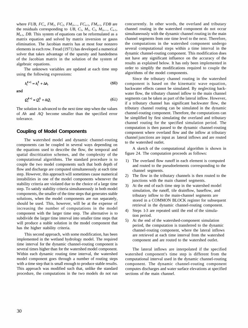
where FUB, FC,, FM1, FC2, FM2,..., FCn-1, FMn-1, FDB are the residuals corresponding to UB, C1, M1, C2, M2,..., Cn-1, Mn-1, DB. This system of equations can be reformulated as a matrix equation and solved by matrix inversion or gauss elimination. The Jacobian matrix has at most four nonzero elements in each row. Fread (1971) has developed a numerical solver that takes advantage of the sparsity and handedness of the Jacobian matrix in the solution of the system of algebraic equations.

The unknown variables are updated at each time step using the following expressions:

The solution is advanced to the next time step when the values of Ah and AQ become smaller than the specified error tolerance.

Coupling of Model Components The watershed model and dynamic channel-routing

components can be coupled in several ways depending on the equations used to describe the flow, the temporal and spatial discritization schemes, and the complexity of the computational algorithms. The standard procedure is to couple the two model components such that both depth of flow and discharge are computed simultaneously at each time step. However, this approach will sometimes cause numerical instabilities in one of the model components whenever the stability criteria are violated due to the choice of a large time step. To satisfy stability criteria simultaneously in both model components, the smaller of the time steps that generates stable solutions, when the model components are run separately, should be used. This, however, will be at the expense of increasing the number of computations in the model component with the larger time step. The alternative is to subdivide the larger time interval into smaller time steps that will produce a stable solution in the model component that has the higher stability criteria.

This second approach, with some modification, has been implemented in the wetland hydrology model. The required time interval for the dynamic channel-routing component is several times higher than for the watershed model component. Within each dynamic routing time interval, the watershed model component goes through a number of routing steps with a time step that is small enough to produce stable results. This approach was modified such that, unlike the standard procedure, the computations in the two models do not run

concurrently. In other words, the overland and tributary channel routing in the watershed component do not occur simultaneously with the dynamic channel routing in the main channel segments from one time level to the next. Therefore, the computations in the watershed component undergo several computational steps within a time interval in the dynamic channel-routing component. This modification does not have any significant influence on the accuracy of the results as explained below. It has only been implemented in order to simplify the modifications required to couple the algorithms of the model components.

Since the tributary channel routing in the watershed component is based on the kinematic wave equation, backwater effects cannot be simulated. By neglecting back­water flow, the tributary channel inflow to the main channel segments can be taken as part of the lateral inflow. However, if a tributary channel has significant backwater flow, the tributary channel routing can be simulated in the dynamic channel-routing component. Therefore, the computations can be simplified by first simulating the overland and tributary channel routing for the specified simulation period. The computation is then passed to the dynamic channel-routing component where overland flow and the inflow at tributary channel junctions are input as lateral inflows and are routed to the watershed outlet.

A sketch of the computational algorithm is shown in figure 24. The computation proceeds as follows:

1) The overland flow runoff in each element is computed and routed to the pseudoelements corresponding to the channel segments.

2) The flow in the tributary channels is then routed to the junctions with the main channel segments.

3) At the end of each time step in the watershed model simulation, the runoff, tile drainflow, baseflow, and tributary inflow to the main-channel segments are stored in a COMMON BLOCK register for subsequent retrieval in the dynamic channel-routing component.

4) Steps 1-3 are repeated until the end of the simula­tion period.

5) At the end of the watershed-component simulation period, the computation is transferred to the dynamic channel-routing component, where the lateral inflows are retrieved at each time interval from the watershed component and are routed to the watershed outlet.

The lateral inflows are interpolated if the specified watershed component's time step is different from the computational interval used in the dynamic channel-routing component. The dynamic channel-routing component computes discharges and water surface elevations at specified sections of the main channel.

30

Figure 24. Wetland hydrologic model

31

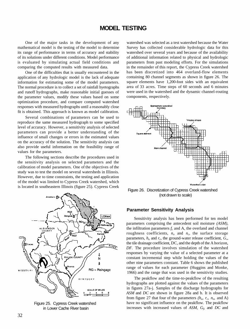
MODEL TESTING

One of the major tasks in the development of any mathematical model is the testing of the model to determine its range of performance in terms of accuracy and stability of its solutions under different conditions. Model performance is evaluated by simulating actual field conditions and comparing the computed results with measured data.

One of the difficulties that is usually encountered in the application of any hydrologic model is the lack of adequate information for estimating some of the model parameters. The normal procedure is to collect a set of rainfall hyetographs and runoff hydrographs, make reasonable initial guesses of the parameter values, modify these values based on some optimization procedure, and compare computed watershed responses with measured hydrographs until a reasonably close fit is obtained. This approach is known as model calibration.

Several combinations of parameters can be used to reproduce the same measured hydrograph to some specified level of accuracy. However, a sensitivity analysis of selected parameters can provide a better understanding of the influence of small changes or errors in the estimated values on the accuracy of the solution. The sensitivity analysis can also provide useful information on the feasibility range of values for the parameters.

The following sections describe the procedures used in the sensitivity analysis on selected parameters and the calibration of model parameters. One of the objectives of the study was to test the model on several watersheds in Illinois. However, due to time constraints, the testing and application of the model was limited to Cypress Creek watershed, which is located in southeastern Illinois (figure 25). Cypress Creek

Figure 25. Cypress Creek watershed in Lower Cache River basin

watershed was selected as a test watershed because the Water Survey has collected considerable hydrologic data for this watershed over several years and because of the availability of additional information related to physical and hydrologic parameters from past modeling efforts. For the simulations in the remainder of this report, the Cypress Creek watershed has been discretized into 464 overland-flow elements containing 80 channel segments as shown in figure 26. The square elements have 1,200-foot sides with an equivalent area of 33 acres. Time steps of 60 seconds and 6 minutes were used in the watershed and the dynamic channel-routing components, respectively.

Figure 26. Discretization of Cypress Creek watershed (not drawn to scale)

Parameter Sensitivity Analysis

Sensitivity analysis has been performed for ten model parameters comprising the antecedent soil moisture (ASM), the infiltration parameters fc and A, the overland and channel roughness coefficients, no and nc, the surface storage parameters, hu and rc, the ground-water release coefficient, G,, the tile drainage coefficient, DC, and the depth of the A horizon, DF. The procedure involves simulation of the watershed responses by varying the value of a selected parameter at a constant incremental step while holding the values of the other nine parameters constant. Table 6 shows the published range of values for each parameter (Huggins and Monke, 1966) and the range that was used in the sensitivity studies.

The peakflow and the time-to-peakflow of the resulting hydrographs are plotted against the values of the parameters in figures 27a-j. Samples of the discharge hydrographs for ASM and DC are shown in figure 28a and b. It is observed from figure 27 that four of the parameters (hu, rc, no, and A) have no significant influence on the peakflow. The peakflow increases with increased values of ASM, Gf, and DC and

32

decreases as DF, nc, and fc increase. The time-to-peakflow increases as the values of Gf, DF, and nc increase and decreases with increasing DC. However, the trends in the variation of the time-to-peakflow are not uniform for ASM, no and fc. Moreover, the time-to-peak is insensitive to variations in hu, rc, and A.

Table 6. Range of Parameters for Sensitivity Analysis Published range Range of

Parameters of values values used ASM 0.31 - 1.0 0.35 - 0.9 Gf 0.0 - 0.01 0.0 - 0.01 hu (inches) 0.5 - 12.0 0 .5 -8 rc 0.25 - 0.8 0.2 - 0.8 DF (inches) 0.25 - 0.75 of a horizon 2 - 14 DC (inches/day) 0.25 - 0.5 0.1 - 0.7 no 0.01 - 0.5 0.01 - 0.5 nc

— 0.02 - 0.3 fc (inches/hour) 0.31 - 0.89 0.3 - 0.9 A (inches/hour) — 0.2 - 0.8

Model Calibration

The objective of the model calibration is to test model performance by comparing computed and measured hydrographs. Three storm events between 1990 and 1991 were selected based on availability of complete precipitation records and corresponding discharge hydrographs. The model

calibration involved an iterative procedure whereby selected model parameters were manually adjusted in incremental steps until the computed hydrograph closely matched observed data. The accuracy of the estimation was evaluated by calculating the standard error, STDERR, and the coefficient of model fit, ERR, as shown in table 7. The standard error is described by:

where Qc(i), Qo(i) are, respectively, computed and observed discharges at time i, and n is the number of time intervals.

The coefficient of model fit, proposed by Nash and Sutcliffe (1971), provides a numerical measure of the efficiency of the calibration. It is described by the follow­ing equation:

where Qavg is the average observed discharge. The hydraulic and hydrologic parameters in the wetland

hydrology model have been grouped into four categories for the purpose of the calibration: 1) soil infiltration and drainage parameters, 2) ground-water release constants, 3) surface storage and roughness coefficients, and 4) channel rough­ness coefficient.

Figure 27. Variation of peakflow and time-to-peakflow to changes in a) ASM, b) G,, c) hu, d) rc, e) DF, f) DC, g) no, h) nc, i) fc, and j) A

33

Figure 27. Concluded

Table 7. Calibration of Infiltration and Ground-Water Release Parameters

Standard Percent Storm date Gf ß fc error efficiency

02/02/89 0.055 0.85 0.83 4.23 92.06 01/19/90 0.095 0.72 0.83 3.36 92.44 05/13/90 0.046 0.84 0.83 2.47 96.49

Soil Infiltration/Drainage Parameters

The soil infiltration and drainage parameters include the steady-state infiltration capacity, fc, the difference between maximum infiltration and steady-state infiltration capacities, A, total porosity, Tp, antecedent soil moisture, ASM, field capacity, F , infiltration exponent, p, and the depth of the A horizon. The values of some of these parameters are obtained

from tables while others are obtained from model calibration. Tp, Fp, and p are estimated using table 5. The depth of the A horizon, DF, for the given soil types was estimated from the USDA soil survey manuals. Since no information is available on the antecedent soil conditions for the three storms, ASM was initially set equal to F for each storm. These estimates were found to be satisfactory for the storm events.

Since sensitivity analysis has shown that fc and A have significant influence on the simulation results, their values were estimated through model calibration. However, the initial estimates for fc and A were obtained using the procedure developed by Beasley and Huggins (1982). By using the range of permeabilities for a given soil type, obtained from the USDA soil survey manuals, 1) fc is estimated as the midpoint of the lower one-third

of the range, and 2) the maximum infiltration capacity is assumed to be

the midpoint of the upper two-thirds of the range.

34

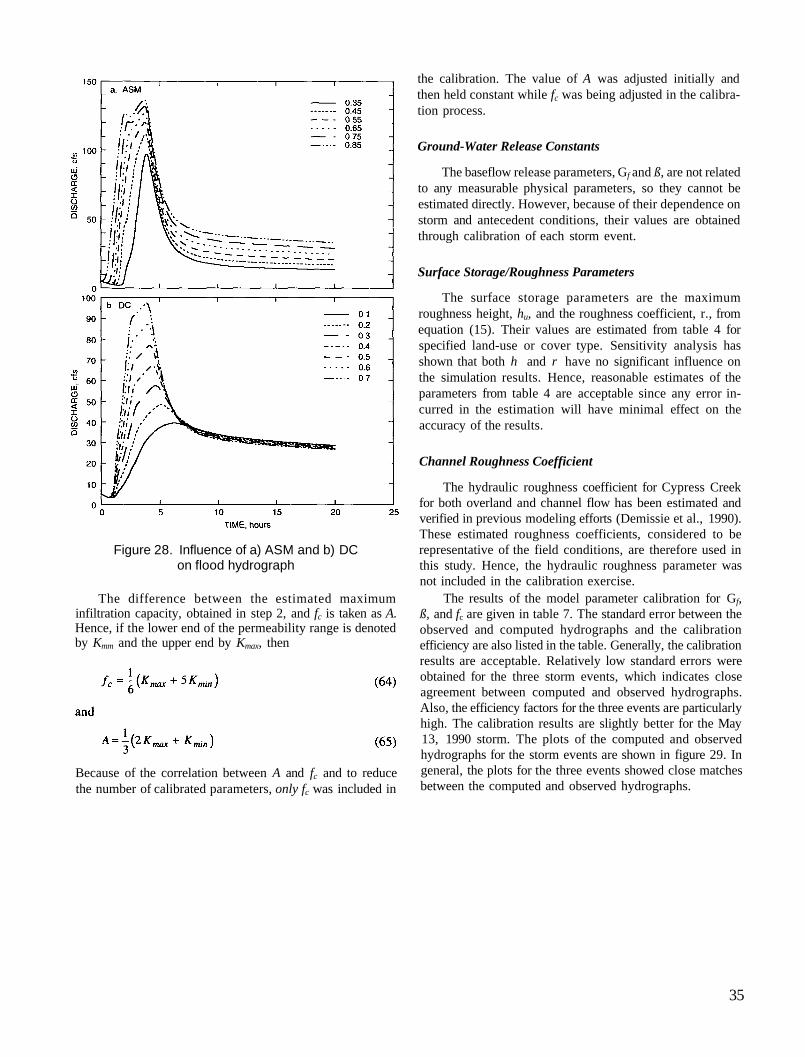
Figure 28. Influence of a) ASM and b) DC on flood hydrograph

The difference between the estimated maximum infiltration capacity, obtained in step 2, and fc is taken as A. Hence, if the lower end of the permeability range is denoted by Kmm and the upper end by Kmax, then

Because of the correlation between A and fc and to reduce the number of calibrated parameters, only fc was included in

the calibration. The value of A was adjusted initially and then held constant while fc was being adjusted in the calibra­tion process.

Ground-Water Release Constants

The baseflow release parameters, Gf and ß, are not related to any measurable physical parameters, so they cannot be estimated directly. However, because of their dependence on storm and antecedent conditions, their values are obtained through calibration of each storm event.

Surface Storage/Roughness Parameters

The surface storage parameters are the maximum roughness height, hu, and the roughness coefficient, r., from equation (15). Their values are estimated from table 4 for specified land-use or cover type. Sensitivity analysis has shown that both h and r have no significant influence on the simulation results. Hence, reasonable estimates of the parameters from table 4 are acceptable since any error in­curred in the estimation will have minimal effect on the accuracy of the results.

Channel Roughness Coefficient

The hydraulic roughness coefficient for Cypress Creek for both overland and channel flow has been estimated and verified in previous modeling efforts (Demissie et al., 1990). These estimated roughness coefficients, considered to be representative of the field conditions, are therefore used in this study. Hence, the hydraulic roughness parameter was not included in the calibration exercise.

The results of the model parameter calibration for Gf, ß, and fc are given in table 7. The standard error between the observed and computed hydrographs and the calibration efficiency are also listed in the table. Generally, the calibration results are acceptable. Relatively low standard errors were obtained for the three storm events, which indicates close agreement between computed and observed hydrographs. Also, the efficiency factors for the three events are particularly high. The calibration results are slightly better for the May 13, 1990 storm. The plots of the computed and observed hydrographs for the storm events are shown in figure 29. In general, the plots for the three events showed close matches between the computed and observed hydrographs.

35

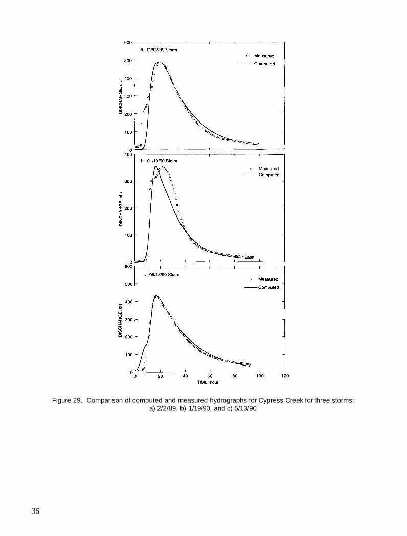
Figure 29. Comparison of computed and measured hydrographs for Cypress Creek for three storms: a) 2/2/89, b) 1/19/90, and c) 5/13/90

36

WETLAND HYDROLOGY AND WATERSHED RESPONSES

The perception of wetlands as wastelands has changed in recent years as scientists have demonstrated the functional values of wetlands. The evaluation of the cumulative impact of the modification of wetlands by natural processes, human activities, or both has involved several qualitative studies, including Carter et al. (1978), Cowardin et al. (1979), O'Brien (1988), Novitzki (1978), and Winter (1988), among others. However, more recent investigations have focused on quanti-fying the impact of the alteration of wetland characteristics on the overall hydrologic responses of the watershed. Of particular interest are those studies involving the application of mathematical models to simulate hydrologic conditions resulting from the impact of wetland modifications.

Two approaches have been used for wetland simulation studies. One approach focuses on the simulation of hydro-logic responses within individual wetlands and at the wetland outlet due to changes in hydrologic and landscape characteristics of the wetland. However, since the effect of changes in wetland characteristics propagates downstream of the wetland outlet, a watershed simulation approach is generally more suitable for studying the cumulative impact of wetland alterations. The former approach was used by Haan and Johnson (1968) in the development of a model to simulate the hydrology of depressional areas and to study the influence of surface roughness and storm patterns on the outflow hydrographs. Also, Hammer and Kadlec (1986) and Kadlec (1990) developed a physically based mathematical model for overland flow through vegetated areas using a modified frictional resistance formula to account for vertical variation of the vegetation density and the spatial variation of the ground surface slope. Ogawa and Male (1986) adopted the latter approach in analyzing several records from existing wetland sites in order to evaluate the effect of wetland encroachment on peak flood flow.

The wetland hydrology model, which has been developed and tested in this study, is based on the watershed simulation approach. However, unlike Ogawa and Male's study, the model uses a distributed-parameter concept whereby hydrologic processes are described by physically based parameters that are allowed to vary both spatially and temporally within the watershed. This approach provides the flexibility of differentiating the hydrologic processes that distinguish a wetland from other areas of the watershed. This is accomplished by selecting appropriate values of relevant parameters to represent the hydrologic condition of the wetland. It is, therefore, possible to evaluate the effects of short- and long-term changes in the hydrologic characteristics on the overall hydrologic response of the watershed.

To determine the impact of wetland dynamics on the hydrologic responses of a watershed, hydrologic variables related to the watershed discharge hydrograph were selected. For a preliminary analysis, the relative magnitude of the peakflow has been used in this chapter to analyze the hydro-

logic responses of a watershed to the dynamic changes in the wetlands located within the Cypress Creek watershed boundaries. The results of this analysis are presented after a discussion of the representation of the hydrologic characteristics of a wetland in the wetland hydrology model.

Representation of Wetland Characteristics Wetlands can be classified into two broad categories:

Coastal wetlands and inland wetlands. Other classifications exist, but the present classification is adequate for the purpose of identifying the hydrologic and physiographical char­acteristics of wetlands. Within each of the two categories are different types and classes of wetlands. Our focus in this study has been on inland wetlands with particular emphasis on the wetlands in the state of Illinois. Inland wetlands are found on floodplains along rivers and waterways, in dry land around depressions and potholes, and along the fringes of ponds and lakes. Examples of these types of wetlands include marshes, wet meadows, shrub swamps, and wooded swamps. The locations of these wetlands span the transitional zone between aquatic and terrestrial systems. The water table is normally a few inches below the ground surface, or the ground surface may be inundated by shallow water.

Wetlands have been defined under section 404 of the Clean Water Act as "those areas that are inundated or saturated by surface or ground water at a frequency and duration sufficient to support, and that under normal circumstances do support, a prevalence of vegetation typically adapted for life in saturated soil conditions." Based on this definition and on the prevalent natural conditions in different types of wetlands, the three basic characteristics of any wetland are:

1) Nearly or fully saturated soil moisture conditions or inundation by shallow water for an extended period

2) Poorly drained and water-retaining soils 3) Water-loving plants prevalent in hydric soils

A saturated soil moisture condition is represented in the wetland hydrology model by setting the antecedent soil moisture conditions to complete saturation.

A ponding condition is modeled by setting the parameter, DIRM, to the anticipated maximum increase in water depth in the wetland. DIRM is the depth of water that must be satisfied in a microrelief before runoff commences. A DIRM value of 2.0 inches is used in elements representing wetland areas compared to 0.02 inches for nonwetland elements. Also, hu= 0 is used to represent a flat surface in the wetland elements so that infiltration occurs over the entire element when rain starts. Once the depth of water is above DIRM, the excess rainfall is routed through the pond. A Manning roughness coefficient of 0.35 is used for overland flow in the wetland elements and a value of 0.085 for nonwetland areas. The effect of the vertical distribution of hydraulic resistance due to the wetland vegetation is considered to be negligible at this stage of the model development.

37

Since a less permeable soil layer is usually found on the wetland bed, the infiltration of water through the bed will be slower even if the initial condition is partially saturated soils. This condition is represented by setting the value of the infiltration capacity in the wetland elements to half the value used for nonwetland elements. Infiltration parameter A is slightly reduced for the wetland areas. Typical model parameter values for wetland and nonwetland areas are shown in table 8.

Table 8. Typical Values of Parameters for both Wetland and Nonwetland Areas

Parameter Wetland area Nonwetland area

Fp (% saturation) 0.72 0.96 fc (inches/hour) 0.23 0.12

A (inches/hour) 0.3 0.25 ASM (% saturation) 0.71 0.96 PIT (inches) 0.01 0.07 hu (inches) 1.755 0.0 rc 0.45 1.0 DIRM (inches) 0.02 2.0 no 0.085 0.35 Gf 0.005 0.005 DF (inches) 3.5 3.5 DC (inches/day) 0.0 0.0 nc * *

Note: * indicates nc values of 0.025, 0.04, and 0.08.

Evapotranspiration is the only other process that has not been included in the current version of the wetland hydrologic model. It will be assumed in all the simulations described in the following section that the effect of evapotranspiration on the wetland open-water surface has been included in the value of DIRM used for the wetland elements.

Influence of Wetlands on Watershed Hydrologic Responses

One of the primary objectives of this study was to examine the impact of changes in wetland areas on peakflow and time-to-peakflow. The wetland model was applied to Cypress Creek watershed for this analysis. One inch of rainfall over the watershed for a duration of one hour was assumed. Wetland areas varying from 10 to 70 percent of the watershed area were assumed. The values of the parameters used for both wetland and nonwetland areas of the watershed are shown in table 8. Several simulation runs were made, and discharge hydrographs were calculated at the watershed outlet. The computed hydrographs for 0, 20, 40, and 70

percent wetland area are compared in figure 30. The results show the attenuation of the flood hydrograph resulting from changes in wetland percentage.

The resulting change in relative peakflow at the watershed outlet due to change in wetland area is plotted in figure 31 for each percentage of wetland area. The relative peakflow is computed as the ratio of the peakflow corresponding to an assumed wetland area in the watershed to the peakflow with no wetland in the watershed. Areas with a higher percentage of wetlands were observed to have more influence on relative peakflow than areas with a lower percentage of wetlands. This is consistent with the results of a previous study by Demissie and Khan (1993), which showed reduction of peakflow with increasing area for Illinois watersheds.

Figure 30. Comparison of discharge hydrographs for different percent wetland at the watershed outlet

Figure 31. Variation of relative peakflow with increasing percent wetland at the watershed outlet

38

SUMMARY AND CONCLUSIONS

The primary goal of this project was to develop and apply a physically based hydrologic and hydraulic model that simulates the hydrologic responses of a watershed having different types and sizes of wetlands at different locations. The approach used in the model development was to select some existing hydrologic and hydraulic models that have been tested and verified. The selected model components were modified to make the modeling approaches suitable for simulating the hydrology of wetlands and the hydrologic responses of the watershed in which the wetlands are situated.

After conducting an extensive literature review of existing hydrologic and hydraulic models, it was concluded that there is no single model with all the attributes needed to simulate the physical processes governing the hydrology of wetlands and their influence on the hydrology of the watershed containing them. It was therefore necessary to select desirable components from some of the reviewed models and combine them to form the base model for the wetland hydrology model. The base model can be improved by incorporating additional components from other models or developing new ones as necessary.

A watershed component and a channel-routing component were selected from two models to form the base model. For the watershed model component, it was decided mat a physically based model is necessary to adequately depict the physical processes in the wetland. Among the 21 models examined, the possible choices for the watershed component were ANSWERS, VSAS2, the Freeze model, SHE, and IHDM. Based on such factors as the input data requirement, computing cost, documentation, and the hydrologic processes modeled, the ANSWERS model was found to offer the best framework for developing the watershed component of the wetland hydrology model.

Since many wetlands are located along me banks and floodplains of streams, the structure of the channel-routing component of the base model should be capable of accounting for variable channel geometry and flow resistance along the longitudinal profile and across the floodplain cross section. A survey of the channel-routing component in each of the 21 watershed models revealed that most models do not have the capability to include variable channel characteristics. Three programs used for calculating surface water profiles satisfy this criterion. However, they assume steady-state conditions and thus cannot be used directly for flood routing in the wetland hydrology model. A dynamic wave model, DWOPER, was also evaluated and found to possess many of the characteristics necessary for detailed flood routing. The DWOPER model was ultimately selected for the channel-routing component of the wetland hydrology model.

Therefore, the base model for the wetland hydrology model uses ANSWERS for the watershed component and DWOPER for the channel-routing component. The channel-routing algorithm in ANSWERS, which is based on kinematic wave assumption, was retained since the kinematic wave model is adequate for channel flow routing in the watershed, where lateral variations in channel characteristics are not important. The coupling of ANSWERS with DWOPER as the base wetland hydrology model was successfully implemented along with a variable grid algorithm that enables a finer grid to be placed anywhere on the watershed, including wetland areas, in order to improve the representation of the physical processes in those areas.

Time constraints did not permit the implementation of some of the other proposed modifications to the base wetland hydrology model. These modifications include the incorporation of the Penman's evapotranspiration equation as used in the MMDW model, the replacement of me Holtan's equation in ANSWERS with the Green-Ampt equation as used in CREAMS, the incorporation of depression storage and routing relations and the Kirkham's tile drainage formula as used in the MMDW model, and the replacement of the empirical baseflow equation with the planar ground-water flow model, PLASM. These and other modifications will be addressed in the future as we continue to improve the model.

The current version of the wetland hydrology model can be used to evaluate the hydrologic response of any watershed. However, it should be noted mat the model has been tested and applied only to the Cypress Creek watershed, which is located in the Cache River basin in southern Illinois. There are plans to select test watersheds in other parts of Illinois and to further test the model. The wetland hydrology model was calibrated using three storm events in the Cypress Creek watershed until the results showed a close fit between the computed and measured hydrographs. The model was then applied to evaluate the hydrologic responses of the Cypress Creek watershed to changes in wetland size. The modeling results indicate mat the role of wetlands in peak flood flow reduction is relatively significant, with a higher rate of change in peakflow for wetland areas up to 60 percent of the Cypress Creek watershed. Results also show that the influence of a wetland diminishes with distance from the wetland outlet.

The results from the present study should be considered preliminary and should not be generalized for all watersheds in Illinois until the hydrologic model is tested on several watersheds in the state. More definitive quantification of the relationship between the watershed response variables, such as peakflow and runoff volume, and the landscape and hydrologic characteristics of wetlands will require both verification of the model for different watersheds in the region and more research.

39

REFERENCES Abbott, M.B., J.C. Bathurst, J.A. Cunge, RE. O'Connell, and

J. Rasmussen. 1986. An Introduction to the European Hydrological System— Systeme Hydrologique Europeen, "SHE," 2: Structure of a Physically-Based, Distributed Modelling System. Journal of Hydrology 87:61-77.

Amein, M.M. and C.S.Fang. 1970. Implicit Flood Routing in Natural Channels. Journal of Hydraulics Division, ASCE 96, No. HY12, December.

Beasley, D.B. 1977. ANSWERS: A Mathematical Model for Simulating the Effects of Land Use and Management on Water Quality. Ph.D. thesis, Purdue University, West Lafayette, IN.

Beasley, D.B., and L.F. Huggins. 1982. ANSWERS: User Manual. Great Lakes National Program Office, U.S. EPA-905/9-82-001, p. 54.

Bernier.P.Y. 1982. VSAS2: A Revised Source Area Simulator for Small Forested Basins. Ph.D. thesis, University of Georgia, Athens, GA.

Bouwer, H., and J. Van Schilfgaarde. 1963. Simplified Method of Predicting Fall of Water in Drained Land. Transactions of the American Society of Agricultural Engineering 6(4):288-291.

Broadhead, R.G., and R.W. Skaggs. 1984. Hydrologic Effects of Peat Mining. Paper No. 84-2068, American Society of Agricultural Engineering, St. Joseph, MI.

Bureau of Reclamation, U.S. Department of Interior. 1967. Guide for Application of Water Surface Profile Computer Program. Office of Chief Engineer, Denver, CO.

Campbell, K.L., and H.P. Johnson. 1975. Hydrologic Simulation of Watersheds with Artificial Drainage. Water Resources Research 11(1):120-126.

Carter, V., M.S. Bedinger, R.P. Novitzki, and W.O. Wilen. 1978. Water Resources and Wetlands. In P.E. Greeson, J.R. Clark, and J.E. Clark (eds.), Wetland Functions and Values: the State of Our Understanding, American Water Resources Association, pp. 367-376.

Chow, V.T., D.R. Maidment, and L.W. Mays. 1989. Applied Hydrology. McGraw-Hill Publishing Company, New York.

Chu, S.C., and C.E. Bowers. 1977. Computer Programs in Water Resources. Water Resources Center Bulletin 97, University of Minnesota, St. Paul, MN.

Clark, C.O. 1945. Storage and the Unit Hydrograph. Transactions of the American Society of Civil Engineers 110:1419-1488.

Cowardin, L.M., V. Carter, F.C. Golet, and E.T. LaRoe. 1979. Classification of Wetlands and Deepwater Habitats of

the United States. Office of Biological Services, U.S. Department of the Interior, FWS/OBS-79/31.

Crawford, N.H. 1971. Studies in the Application of Digital Simulation to Urban Hydrology. Hydrocomp Interna­tional, Inc., Palo Alto, CA.

Crawford, N.H., and R.K. Linsley. 1966. Digital Simulation in Hydrology: Stanford Watershed Model IV. Technical Report 39, Department of Civil Engineering, Stanford University, Stanford, CA.

DeBoer, D.W., and H.P. Johnson. 1971. Simulation of Runoff from Depression Characterized Watersheds. Transactions of the American Society of Agricultural Engineers 14(4):615-620.

Demissie, M., and A. Khan. 1993. Influence of Wetlands on Streamflow in Illinois. Illinois State Water Survey Contract Report 561, Champaign, IL.

Demissie, M., T.W. Soong, and R. Camacho. 1990. Cache River Basin: Hydrology, Hydraulics, and Sediment Transport, Volume 2: Mathematical Modeling. Illinois State Water Survey Contract Report 485, Champaign, IL.

Durgunoglu, A., H.V. Knapp, and S.A. Changnon, Jr. 1987. PACE Watershed Model (PWM): Volume 1, Model Development. Illinois State Water Survey Contract Report 437, Champaign, IL.

Eichert, B.S. 1970. Survey of Programs for Water Surface Profiles. Journal of Hydraulics Division ASCE 96(HY2):547-563.

Fleming, G. 1975. Computer Simulation Techniques in Hydrology. American Elsevier Publishing Company, Inc., NY.

Fread, D.L. 1971. Discussion of Implicit Flood Routing in Natural Channels by M. Amein and C.S. Fang. Journal of the Hydraulic Division, ASCE 97(7):1156-1159.

Fread, D.L. 1978. NWS Operational Dynamic Wave Model. In Verification of Mathematical and Physical Models, Proceedings of the 26th Annual Hydraulic Division Spe­cialty Conference, ASCE, College Park, MD, pp. 455-464.

Fread, D.L. 1985. Channel Routing. In M.G. Anderson and T.P. Burt (eds.), John Wiley and Sons Limited, Hydrological Forecasting, pp. 437-503.

Freeze, R.A. 1971. Three-Dimensional Transient, Saturated-Unsaturated Flow in a Groundwater Basin. Water Resources Research 7(2):347-366.

Green, W.A., and G.A. Ampt. 1911. Studies on Soil Physics, I, The Flow of Air and Water through Soils. Journal of Agricultural Science 4:1-24.

40

Haan, C.T., and H.P. Johnson. 1968. Hydraulic Model of Runoff from Depressional Areas: Part II. Development of the Model. Transactions of the American Society of Agricultural Engineers 11(3): 368-373.

Hammer, D.E., and R.H. Kadlec. 1986. A Model for Wetland Surface Water Dynamics. Water Resources Research 22(13):1951-1958.

Hewlett, J.D., and A.R. Hibbert. 1967. Factors Affecting the Response of Small Watersheds to Precipitation in Humid Areas. In W.E. Sopper and H.W. Lull (eds.), Forest Hydrology, Pergamon Press, Oxford, pp. 275-290.

Holtan, H.N. 1961. A Concept for Infiltration Estimates in Watershed Engineering. Agricultural Research Service Paper 41-51, 25 p.

Holtan, H.N., G.J. Stiltner, W.H. Henson, and N.C. Lopez. 1975. USDAHL-74 Revised Model of Watershed Hydrology. U.S. Department of Agriculture, Agricultural Research Center, Technical Bulletin 1518.

Horton, R.E. 1919. Rainfall Interception. Monthly Weather Review 47:603-623.

Horton, R.E. 1933. The Role of Infiltration in the Hydrologic Cycle. Transactions of the American Geophysical Union 14:446-460.

Horton, R.E. 1939. Analysis of Runoff Plat Experiments with Varying Infiltration-Capacity. Transactions of the American Geophysical Union 20:693-711.

Huggins, L.F., and Monke, E.J. 1966. The Mathematical Simulation of the Hydrology of a Small Watershed. Water Resources Research Center Technical Report 1, Purdue University, West Lafayette, IN.

Huggins, L.F., T.H. Podmore, and C.F. Hood. 1976. Hydrologic Simulation Using Distributed Parameters. Water Resources Research Center Technical Report 82, Purdue University, West Lafayette, IN.

Kadlec, R.H. 1990. Overland Flow in Wetlands: Vegetation Resistance. Journal of Hydraulic Engineering, ASCE 116(5):691-706.

Kirkham, D. 1958. Seepage of Steady Rainfall through Soil into Drains. Transactions of the American Geophysical Union 39:892-908.

Lager, J.A., and W.G. Smith. 1971. Storm Water Management Model, Vol. I. PB-203289, U.S. Environmental Protection Agency, Water Quality Office.

Lefkoff, L.J. 1981. Application of the Variable Source Area Simulator to a Forested Piedmont Watershed. Master's thesis, University of Georgia, Athens, GA.

Liggett, J.A., and J.A.Cunge. 1975. Numerical Methods of Solution of the Unsteady Flow Equations. In Unsteady

Flow in Open Channels, Water Resources Publications, Fort Collins, CO.

Linsley, R.K. 1982. Rainfall-Runoff Models - An Overview. In V.P. Singh (ed.), Rainfall-Runoff Relationship, Water Resources Publications, Littleton, CO, pp. 3-22.

Liou, E.Y. 1970. OPSET: Program for Computerized Selection of Watershed Parameter Values for the Stanford Watershed Model. Water Resources Institute, Research Report 34, University of Kentucky, Lexington.

McCarthy, G.T. 1938. The Unit Hydrograph and Flood Routing. Paper presented at Conference of the North Atlantic Division of U.S. Army Corps of Engineers, New London, CT.

Mein, R.G., and C.L. Larson. 1971. Modeling the Infiltration Component of the Rainfall-Runoff Process. Bulletin No. 43, Water Resources Research Center, University of Minnesota, St. Paul, MN.

Monteith, J.L. 1965. Evaporation and Environment. In The State and Movement of Water in Living Organisms, Proceedings, 15th Symposium, Society for Experimental Biology, Swansea, Cambridge University Press, London.

Moore, I.D., and C.L. Larson 1979. Effects of Drainage Projects on Surface Runoff from Small Depressional Watersheds in the North Central Region. Bulletin No. 99, Water Resources Research Center, University of Minnesota, St. Paul, MN.

Nash, J.E., and J.V. Sutcliffe. 1971. River Flow Forecasting through Conceptual Models, Part I - A Discussion of Principles. Journal of Hydrology 10(3):282-290.

Novitzki, R.P. 1978. Hydrologic Characteristics of Wisconsin's Wetlands and Their Influence on Floods, Stream Flow, and Sediment. In P.E. Greeson, J.R. Clark, and J.E. Clark (eds.), Wetland Functions and Values: the State of Our Understanding, American Water Resources Association, pp. 377-388.

O'Brien, A.L. 1988. Evaluating the Cumulative Effects of Alteration on New England Wetlands. Environmental Management 102(5):627-636.

Ogawa, H., and J.W. Male. 1986. Simulating the Flood Mitigation Role of Wetlands. ASCE, Journal of Water Resources Planning and Management 112(1): 114-128. Overton, D.E. 1965. Mathematical Refinement of an Infiltration Equation for Watershed Engineering. U.S. Department of Agriculture, Agricultural Research Services, pp. 41-99.

Penman, H.L. 1948. Natural Evapotranspiration from Open Water, Bare Soil and Grass. Proceedings, Royal Society of London 193:120-145.

Philip, J.R. 1954. An Infiltration Equation with Physical Significance. Soil Science 77:153-157.

41

Prickett, T.A., and C.G. Lonnquist. 1971. Selected Digital Computer Techniques for Groundwater Resource Evaluation. Illinois State Water Survey Bulletin 55, Champaign, IL.

Richards, L.A. 1931. Capillary Conductivity of Liquid through Porous Media. Physics 1:318-333.

Rockwood, D.M. 1968. Application of Streamflow Synthesis and Reservoir Regulation-SSARR-Program to Lower Mekong River. Publication No. 80, FASIT Symposium, Tucson, AZ.

Rogers, C.C.M., K.J. Beven, E.M. Morris, and M.G. Anderson. 1985. Sensitivity Analysis, Calibration, and Predictive Uncertainty of the Institute of Hydrology Distributed Model. Journal of Hydrology 81:179-191.

Rutter, A.J., K.A. Kershaw, P.C. Robins, and A.J. Morton. 1971/72. A Predictive Model of Rainfall Interception in Forests, 1. Derivation of the Model from Observations in a Plantation of Corsican Pine. Agricultural Meteorology 9: 367-384.

Saint-Venant, B. De. 1871. Theory of Unsteady Water Flow, with Application to River Floods and to Propagation of Tides in River Channels. Paris: Computes Rendus Acad. Sci. 73:148-154, 237-240. Translated into English by U.S. Army Corps of Engineers, No. 49-g, Waterways Experiment Station, Vicksburg, MS, 1949.

Saxton, K.E., P.F. Brooks, R. Richmond, and J.S. Romberger. 1984. Users Manual for SPAW—A Soil-Plant-Air-Water Model. USDA-SEA-AR, unpublished manual.

Saxton, K.E., H.P Johnson, and R.H. Shaw. 1971. Modeling Evapotranspiration and Soil Moisture. Unpublished Paper No. 71-763b, presented at the 1971 Winter Meeting ASAE, Chicago, IL.

Shafer, J.M., and R.L. Skaggs. 1983. Identification and Characterization of Watershed Models for Evaluation of Impacts of Climate Change on Hydrology. Pacific Northwest Laboratory, Richland, WA.

Skaggs, R.W. 1980. A Water Management Model for Artificially Drained Soils. Water Resources Research

Institute Technical Bulletin No. 267, North Carolina State University, Raleigh, NC.

Snyder, F.F. 1938. Synthetic Unit Hydrographs. Transactions of the American Geophysical Union 19(l):447-454.

Soil Conservation Service, U.S. Department of Agriculture. 1973. Computer Program for Project Formulation Hydrology. Technical Release 20.

Thornthwaite, C.W. 1948. An Approach toward a Rational Classification of Climate. Geographical Review 38:55-94.

Troendle, C.A. 1979. A Variable Source Area Model for Stormflow Prediction on First Order Forested Watersheds. Ph.D. dissertation, University of Georgia, Athens, GA.

U.S. Army Corps of Engineers. 1960. Routing of Floods through River Channels. Engineering Manual 1110-2-1408, Washington, D.C.

U.S. Army Corps of Engineers. 1972a. Program Description and Users Manual for SSARR Model Streamflow Synthesis and Reservoir Regulation. Program 724-K5-G0010.

U.S. Army Corps of Engineers. 1972b. HEC-2, Water Surface Profiles, User's Manual 723-02A.

U.S. Army Corps of Engineers. 1985. HEC-1 Flood Hydrograph Package, Users and Programmers Manual 723-X6-L2010.

U.S. Department of Agriculture. 1980. CREAMS: A Field-Scale Model for Chemicals, Runoff, and Erosion from Agricultural Management Systems (W.H. Knisel, ed.). Conservation Research Report 26, 640 p.

U.S. National Weather Service, Office of Hydrology. 1972. Na­tional Weather Service River Forecast System Forecast Procedures. National Oceanic and Atmospheric Adminis­tration Technical Memorandum NWS HYDRO-14.

Williams, J.R., A.D. Nicks, and J.G. Arnold. 1985. Simulator for Water Resources in Rural Basins. Journal of Hydraulic Engineering ll(6):970-986.

Winter, T.C. 1988. A Conceptual Framework for Assessing Cumulative Impact on the Hydrology of Nontidal Wetlands. Environmental Management 102(5):605-620.

42