hydrodynamic lubrication theory in …powers/smith.thesis.pdf5.31 zones of cavitation and no...
TRANSCRIPT

Reproduced with permission of the copyright owner. Further reproduction prohibited without permission.
HYDRODYNAMIC LUBRICATION THEORY IN
ROTATING DISK CLUTCHES
A Dissertation
Submitted to the Graduate School
of the University of Notre Dame
In Partial Fulfillment of the Requirements
for the Degree of
Doctor of Philosophy
by
Andrew M. Smith, B.S., M.S.
Department of Aerospace and Mechanical Engineering
Notre Dame, Indiana
April 1997
---------

Reproduced with permission of the copyright owner. Further reproduction prohibited without permission.
UMI Number: 9722365
UMI Microform 9722365 Copyright 1997, by UMI Company. All rights reserved.
This microform edition is protected against unauthorized copying under Title 17, United States Code.
UMI 300 North Zeeb Road Ann Arbor, MI 48103
---------
Reproduced with permission of the copyright owner. Further reproduction prohibited without permission.
HYDRODYNAMIC LUBRICATION THEORY IN ROTATING DISK CLUTCHES
Abstract
by
Andrew M. Smith
This dissertation is concerned with modeling the friction, load capacity, and tem
perature rise between a pair of rotating disk clutch plates using a hydrodynamic
lubrication model. The lubricating film possesses a temperature dependent viscosity
which significantly affects overall clutch performance. The model can accommodate
an arbitrary film shape. The governing mass, momentum, and energy equations are
simplified using the assumptions of incompressibility, negligible body forces, and a
thin-film assumption. Velocity, pressure, and temperature profiles are obtained using
a marker and cell method and a three-level fully implicit method. These methods were
verified by comparing numerical results to analytical solutions obtained in limiting
cases in which exact solutions exist. Results are presented for (1) the case of a sinu-
soidally varying film thickness, (2) the constant film thickness case, (3) groove studies,
and (4) a conjugate heat transfer problem. As expected for hydrodynamic theory,
the results indicate that predicted friction coefficients (f-LF ~ 0.005 - 0.03) are nearly
an order of magnitude below typical clutch operating conditions (f-LF ~ 0.1 - 0.3).
A limited set of results indicates that, for the constant film case, spatial gradients
in viscosity may be neglected if the bulk viscosity is chosen to satisfy the viscosity
temperature relation using the average temperature. Both the viscosity-temperature
relation and film size have a significant effect on clutch performance.
---------
Reproduced with permission of the copyright owner. Further reproduction prohibited without permission.
Dedication
This dissertation is dedicated to my parents, Mike and Mary, who taught me the
values of diligence and patience.
ii

Reproduced with permission of the copyright owner. Further reproduction prohibited without permission.
TABLE OF CONTENTS
LIST OF FIGURES
LIST OF TABLES
LIST OF SYMBOLS
ACKNOWLEDGMENTS
1 INTRODUCTION
1.1 Description of Clutch Operation.
1.2 Overview of Current Research
1.3 Utility of the Research
1.4 New Contributions ..
2 LITERATURE REVIEW
2.1 Clutch Studies ..... .
2.1.1 Theoretical Models
2.1.2 Experimental Investigations
2.2 Related Mechanical Devices
2.3 Tribological Issues .....
2.3.1 Mineral Oil Rheology ..
2.3.2 Surface Topography. . .
2.4 Related Fluid Mechanics and Heat Transfer Problems .
3 MATHEMATICAL MODEL
3.1 Domain and Variable Definitions
3.2 Conservation Principles. . . . . .
3.3 Constitutive Equations . . . . . .
3.4 Initial and Boundary Conditions .
3.5 Non-Dimensionalization .....
iii
-_._---
vi
ix
x
xv
1
1
3
8
11
14
14
15
17
18
19
19
24
26
28
28
31
33
36
38

Reproduced with permission of the copyright owner. Further reproduction prohibited without permission.
3.5.1 Choice of Scaling ....
3.5.2 Dimensionless Equations
3.5.3 Simplifications......
3.6 Summarized Problem Statement.
3.7 Algebraic Coordinate Transformation .
3.8 Clutch Performance Parameters ...
3.8.1 Radial Volumetric Flow Rate
3.8.2 Normal Load ..
3.8.3 Tangential Forces
3.8.4 Frictional Moment Delivered .
3.8.5 Friction Coefficient . . . . . . .
4 NUMERICAL SOLUTION METHOD
4.1 Staggered Grid ............ .
4.2 Discretized Equations. . . . . . . . . .
4.2.1 Discrete Radial and Angular Momentum
4.2.2 Discrete Poisson Pressure Equation
4.2.3 Discrete Axial Velocity Equation
4.2.4 Discrete Energy Equation ....
4.3 Algorithm Summary . . . . . . . . . . .
4.4 Treatment of Clutch Performance Parameters
4.5 Numerical Verification ......... .
4.5.1 Isoviscous Axisymmetic Solutions
4.5.2 Isoviscous, Radially Grooved Solution .
5 RESULTS
5.1 Model Solution for a Sinusoidally Varying Film Thickness.
5.2 Effects of Variable Viscosity on the Constant Film Thickness Case.
5.3 Groove Studies ..... .
5.3.1 Cavitation Studies
5.3.2 Non-Cavitation Studies.
5.4 Multiple Disk Solutions .....
iv
--------
38
40
43
46
49
52
53
53
54
55
56
57
57
59
60
62
66
69
72
74
75
75
81
87
87
91
109
110
113
116

Reproduced with permission of the copyright owner. Further reproduction prohibited without permission.
6 CONCLUSIONS AND RECOMMENDATIONS
6.1 Discussion of Results
6.2 Recommendations..
6.2.1 Recommendations in Experimental Studies.
6.2.2 Recommendations in Theoretical Studies ..
6.2.3 Boundary and Mixed Film Lubrication Models.
APPENDIX A
APPENDIXB
APPENDIX C
BmLIOGRAPHY
v
- - -- ----
131
............ 131
.......... 134
.. ,. ...... 135
136
138
141
143
145
149

Reproduced with permission of the copyright owner. Further reproduction prohibited without permission.
LIST OF FIGURES
1.1 Simplified Clutch Schematic ......... .
1.2 Simplified Clutch Schematic with Lubrication
1.3 Thermal Model Schematic
1.4 Fluid Model Schematic
1.5 Conjugate Problem Schematic
3.1 Lubrication Problem Domain
3.2 Thermal Problem Domain . .
3.3 Viscosity-Temperature Relation for Seven SAE Oils
4.1 Staggered Grid ................... .
4.2 Numerical and Analytical Pressure Profiles .... .
4.3 (a) Numerical and (b) Analytical Radial Velocity Profiles.
4.4 (a) Numerical and (b) Analytical Angular Velocity Profiles
4.5 (a) Numerical and (b) Analytical Axial Velocity Profiles .
2
3
5
6
13
29
31
35
58
77
78
78
79
4.6 Error Analysis for Isoviscous Axisymmetric Check Case . . 79
4.7 (a) Numerical and (b) Analytical Pressure Profiles using Nr = No = 125 84
4.8 Error Analysis for Isoviscous Radially Grooved Case. . . . . . . . .. 85
5.1 Film thickness profile from Equation 5.2, using Nr = 49, No = 49,
R* = 1.3, (}o = 0.1, and h;o = 1.0. . . . . . . . . . . . . . . . . . 88
5.2 Pressure Profile . . . . . . . . . . . . . . . . . . . . . . . . . . . 89
5.3 Radial Velocity Profiles at (). = (a) 0, (b) ~, (c) ~, and (d) ~. 90
5.4 Angular Velocity Profiles at (). = (a) 0, (b) ~, (c) ~, and (d) ~. 97
5.5 Axial Velocity Profiles at (). = (a) 0, (b) ~, (c) ~, and (d) ~. 98
5.6 Temperature Profiles at ()* = (a) 0, (b) ~, (c) ~, and (d) ~. 99
5.7 Variation of Flow Rate with Outlet Pressure ..
5.8 Variation of Normal Force with Outlet Pressure
5.9 Variation of Tangential Force with Outlet Pressure
5.10 Variation of Friction Torque with Outlet Pressure .
vi
--------
100
100
100
101

Reproduced with permission of the copyright owner. Further reproduction prohibited without permission.
5.11 Variation of Friction Coefficient \\ith Outlet Pressure 101
5.12 Variation of Temperature Rise with Outlet Pressure. 101
5.13 Variation of Flow Rate with Inlet Temperature. . . . 102
5.14 Variation of Normal Force with Inlet Temperature. . 102
5.15 Variation of Tangential Force with Inlet Temperature 102
5.16 Variation of Friction Torque with Inlet Temperature. 103
5.17 Variation of Friction Coefficient with Inlet Temperature. 103
5.18 Variation of Temperature Rise with Inlet Temperature . 103
5.19 Variation of Flow Rate with Relative Angular Velocity . 104
5.20 Variation of Normal Force with Relative Angular Velocity. 104
5.21 Variation of Tangential Force with Relative Angular Velocity . . 104
5.22 Variation of Friction Torque with Relative Angular Velocity " 105
5.23 Variation of Friction Coefficient with Relative Angular Velocity 106
5.24 Variation of Temperature Rise with Relative Angular Velocity . 106
5.25 Variable and Constant Viscosity Pressure Profiles . . . . . . . . 107
5.26 (a) Variable and (b) Constant Viscosity Radial Velocity Profiles 107
5.27 (a) Variable and (b) Constant Viscosity Angular Velocity Profiles 108
5.28 (a) Variable and (b) Constant Temperature Profiles . . . . . . . . 108
5.29 (a) Film Thickness Schematic in (). - z. plane and (b) Film Thickness
with Xl = 0.4, X2 = 0.2, R. = 1.3, (}o = 0.1 rad, h~ = 3.5. ...... 110
5.30 (a) Typical Pressure Distribution and (b) Pressure Contours. (Using
S = 968.72 and h; = 3.5.) ....... 112
5.31 Zones of Cavitation and No Cavitation 11-1
5.32 Maximum Pressure vs. Groove Depth. 114
5.33 Normal Load vs. Groove Depth and Sommerfeld Number. 115
5.34 Normal Load vs. Groove Depth using Variable and Constant Viscosity 115
5.35 Velocity Vectors at Average Clutch Radius . . . . . . . . . . . . . .. 116
5.36 Multiple Disk Clutch Conjugate Model Schematic . . . . . . . . . .. 11 i
5.37 Comparison Between Numerical and Analytical Assembly Tempera-
ture Distributions at r = Ro using constant viscosity, E.i = 1, and Po
~ = O .......•.•.......•.....•.......... " 123
vii
- ---------

Reproduced with permission of the copyright owner. Further reproduction prohibited without permission.
5.38 Numerical Assembly Temperature Distributions at r = Ro with con-
t t · 'ty 2.i - 2 d ~ - 0 san VlSCOSI, - ,an h - •••••••••••••••.•••• po 0 124
5.39 Numerical Assembly Temperature Distributions at r = Ro and () = 0
'th t t' 'ty 2.i 2 d ~ 0 5 WI cons an VlSCOSI, =, an h = . . . . . . . . . . . . . . . . Po 0
125
5.40 Numerical Assembly Temperature Distributions at r = Ro with vari-
bl . 't 2.i - 2 d ~ - 0 a e VlSCOSI y, -, an h - • . • • • • • • • • • • • • • • • • • • • po 0
126
5.41 Numerical Assembly Temperature Distributions at r = Ro and () = 0
'th . bl . 't 2.i - 2 d ~ - 0 -WI vana e VlSCOSl y, -, an h - .0 ..•...•........ po 0
130
viii
Reproduced with permission of the copyright owner. Further reproduction prohibited without permission.
LIST OF TABLES
1.1 LUBRICATION REGIMES (A = sU~A~rr5J<~~ss) ....... " 10
3.1 RESULTS FROM FITTING SHIGLEY'S DATA INTO WALTHERS'S
EQUATION . . . . . . . . . . . . . . . . . . . . . ......... " 34
3.2 TYPICAL CLUTCH OPERATING CONDITIONS . . . . . . . . .. 43
3.3 RANGE OF PARAMETERS STUDIED .............. " 44
3.4 TYPICAL CLUTCH DIMENSIONLESS PARAMETERS. . . . . .. 44
3.5 RANGE OF DIMENSIONLESS PARAMETERS STUDIED ... " 44
5.1 CONSTANT PARAMETERS FOR RESULTS PRESENTED IN SEC-
TION 5.1 ................................. 89
5.2 CONSTANT PARAMETERS FOR RESULTS PRESENTED IN SEC-
TION 5.2 ................................. 92
5.3 MAXIMUM VALUES OF TERMS IN DIMENSIONLESS ENERGY
EQUATION. . . . . . . . . . . . . . . . . . . . . . . . . . . . . . .. 95
5.4 COMPARISON BETWEEN CONSTANT AND VARIABLE VISCOS-
ITY PREDICTIONS FOR THE CONSTANT FILM CASE (CV: CON
STANT VISCOSITY BASED ON AVERAGE TEMPERATURE PRE
DICTED THROUGHOUT DOMAIN, VV: WORKING VARIABLE
VISCOSITY MODEL) . . . . . . . . . . . . . . . . . . . . . . . . .. 127
5.5 CONSTANT PARAMETERS FOR RESULTS PRESENTED IN SEC-
TION 5.3.1 .......... . . . . . . . . . . . . . . . . . . . . .. 128
5.6 CONSTANT PARAMETERS FOR RESULTS PRESENTED IN SEC-
TION 5.3.2 ................................ 128
5.7 RESULTS FOR SECTION 5.3.2 (VV - VARIABLE VISCOSITY, CV
- CONSTANT VISCOSITY) . . . . . . . . . . . . . . . . . . . . . .. 129
5.8 CONSTANT PARAMETERS FOR RESULTS PRESENTED IN SEC-
TION 5.4 ........... . . . . . . . . . . . . . . . . . . . . .. 129
5.9 SUMMARY OF CLUTCH PERFORMANCE (VV - VARIABLE VIS
COSITY, CV - CONSTANT VISCOSITY) . . . . . . . . . . . . . .. 130
ix
~~-~----
Reproduced with permission of the copyright owner. Further reproduction prohibited without permission.
LIST OF SYMBOLS
- Accent denoting computational integral quantity
i Accent denoting computational variables
-* Subscript denoting dimensionless quantities
-b, -" -s Subscript denoting backing, friction, and separator materials
-min, -max Subscript denoting minimum and maximum values of quantities
-* Superscript denoting dimensionless quantities
-[ 1 Superscript with argument denoting discrete grid location
aIT, azr, a3T, Coefficients of discrete energy equation
c
e
Coefficients for differential form of continuity equation
Coefficients of Poisson pressure equation
Constants for isoviscous axisymmetric solution
Specific heat of material region of interest [k: K] Internal energy per unit mass [~]
Hypothetical right hand side of continuity equation
Forcing function for Poisson pressure equation
x

Reproduced with permission of the copyright owner. Further reproduction prohibited without permission.
fVr
iVr
iT
iVD
ivz fVB
iVB
fVBBC
h
i,j, k
k
m
n
n
P
Pi
Po
r
s
t
Discrete vector form of radial momentum forcing function
Scalar kernel form of radial momentum forcing function
Forcing function of discrete energy equation
Viscous dissipation term in energy equation
Forcing function for differential form of continuity
Discrete vector form of angular momentum forcing function
Scalar kernel form of angular momentum forcing function
Discrete vector form of angular momentum boundary conditions
Film thickness [m]
Groove depth [m]
Minimum film thickness [m]
Convective heat transfer coefficient [mf K] Indices denoting discrete radial, angular, and a..xial location
Thermal conductivity [~VK]
Vector of length Nz containing elements equal to zero or one
Viscosity-temperature parameter
Index representing any integer
Unit outward normal
Pressure [~]
Pressure difference, Pi - Po [~]
Pressure at inner radius [::'2] Pressure at outer radius [::'2] Cylindrical heat flux vector components ['*] Radial coordinate [m]
Local location along surface roughness trace [m]
Time [s]
Xl

Reproduced with permission of the copyright owner. Further reproduction prohibited without permission.
w
X,Y
z
z'
A
A
A
B
EHL
FO,Q
FO,h
Gr
J
L
Cylindrical velocity components [r:] Discrete vector form of radial and angular velocity
Discrete weighted vector for numerical integration
General discrete vectors
Axial coordinate [m]
Global axial coordinate for multiple disk clutch solutions [m]
Viscosity-temperature parameter [Km]
Tridiagonal matrix
General block-banded matrix
Viscosity-temperature parameter [:;:~]
Viscosity-temperature parameter ["'a2]
Brinkman number
Elastohydrodynamic lubrication
Tangential force due to pressure [N]
Normal load [N]
Tangential force due to viscous shearing on separator plate [N]
Tangential force due to viscous shearing on friction plate [N]
Graetz number
Input side mass moment of inertia [kg m2]
Output side mass moment of inertia [kg m2]
Numerical approximation of integral of radial velocity component
Ratio of fluid inertia to clutch inertia
Jacobian matrix
Viscosity-temperature parameters
Axial length of material regions [m]
xu

Reproduced with permission of the copyright owner. Further reproduction prohibited without permission.
Nr,N(J,Nz
Pr
Qr
Q(J
R.
~
Ro
Re
S
SAE
SUV
T
Tre[
Z
Length of surface roughness measurement [m]
Input side moment [N m]
Output side moment [N m]
Moment due to clutch friction [N m]
Total number of periodic domains on clutch friction plate
Number of radial, angular, and axial grid points
Prandtl number
Volumetric flow rate in radial direction ["'s3]
Volumetric flow rate per unit depth in azimuthal direction ["'s2]
Ratio of outer to inner clutch radii
Inner clutch radius [m]
Outer clutch radius [m]
Reynolds number
Sommerfeld number
Society of Automotive Engineers
Saybolt universal viscosity
Temperature [K]
Nodal average temperature [K]
Ambient temperature [K]
Radial inlet temperature [K]
Reference temperature [K]
Local height of surface measured from mean height [m]
Thermal diffusivity of material region of interest ["'s2]
Coefficients in isoviscous radial grooved solution
Ratio of minimum film thickness to inner radius
xiii

Reproduced with permission of the copyright owner. Further reproduction prohibited without permission.
f)
J.LF
J.La
J.Lre/
v
p
Angular coordinate [rad]
Domain angle of periodicity [rad]
Convective partial derivative coefficients in energy equation
Viscosity [!fnf] Coefficient of friction
Radial inlet viscosity [~:]
Reference viscosity [!fnf] Kinematic viscosity ["'s2]
Density of material region of interest [~]
Root mean square surface roughness [m]
Cylindrical tress tensor components [~]
Xl, X2 Geometric groove parameters
r n Constant in isoviscous radial grooved solution
b..f, b..1J, b..i Radial, angular, and axial grid spacings
A Ratio of minimum film thickness to surface roughness
Od Relative angular velocity of separator plate [r~d]
O. Ratio of relative angular velocity to input angular velocity
0 1 Input side angular velocity [r~d]
O2 Output side angular velocity [r~d]
xiv
- ---- -----

Reproduced with permission of the copyright owner. Further reproduction prohibited without permission.
ACKNOWLEDGMENTS
I would like to acknowledge my advisors, Dr. Kwang-Tzu Yang and Dr. Joseph M.
Powers, for the opportunity they have given me, their interest in this material, and
their endless pursuit of excellence. I would also like to acknowledge my committee
members, Dr. Steven R. Schmid, Dr. Samuel Paolucci, Dr. Mihir Sen: and Dr. Albin A.
Szewczyk, not only for serving on my committee, but for the educational experiences
they have given me. Additional professors at the University of Notre Dame who have
inspired my academic pursuits by giving me a broader perspective of the physical and
philosophical world include Dr. Robert A. Howland, Dr. James J. Mason. and Dr.
Michael M. Stanisic.
I would like to acknowledge Clark-Hurth Components for their sponsorship dur
ing most of my graduate career. Specifically, Mr. Hormuz Kerendian and Mr. Rick
Honeyager were actively involved in this research.
I would like to acknowledge several of the University of Notre Dame's Aerospace
and Mechanical Engineering graduate students for their advice, friendship, and over
all companionship: Tom Copps, Keith Gonthier, Rich Sellar, George Ross: Elgin
Anderson, Matt Grismer, Rob Minitti, Dave Williams, Ken Cheung, Keith Roessig,
and Chris Sullivan. I would also like to mention several close friends who have di
rectly, and indirectly, influenced my educational experiences. I have the pleasure of
knowing Felix Kpodo, Mike Cambi, Steve Ryan, John Hanzas, Dan Gabriel, Osiris
Gabiam, Jerry Bodine, John Boburka, Mike Connel, Jim Primich, Pete Quast: Diana
DiBeradino, Paul Perl, Christine Vogt, Paul Vogt, Mark Heilman, and Ann Heilman.
In particular, I wish to thank Sarah Dakin, for her love, compassion, and friendship.
Finally, I would like to thank my family for their constant support and love; my
parents, Mike and Mary, my brothers, Steve and Tom, my sister and her husband,
xv
- --------

Reproduced with permission of the copyright owner. Further reproduction prohibited without permission.
Evelyn and Chuck, and my grandparents, James and Myra.
xvi
-------

Reproduced with permission of the copyright owner. Further reproduction prohibited without permission.
CHAPTER 1
INTRODUCTION
This dissertation will apply hydrodynamic lubrication theory to model the behav
ior of disk clutches. In particular, this research considers a thin film of lubricant oil
between a pair of rotating disk clutch plates. This oil is capable of supporting load,
transmitting a shear stress, and sustaining large temperature rises induced by viscous
dissipation. Using the disciplines of fluid mechanics and heat transfer, the velocity,
pressure, and temperature fields are predicted in the lubricant and the surrounding
plates. These distributions may be used to predict normal loads, frictional moments,
volumetric flow rates, friction coefficients, and heat generated between clutch plates.
1.1 Description of Clutch Operation
A clutch is a mechanical device designed for engaging and disengaging two working
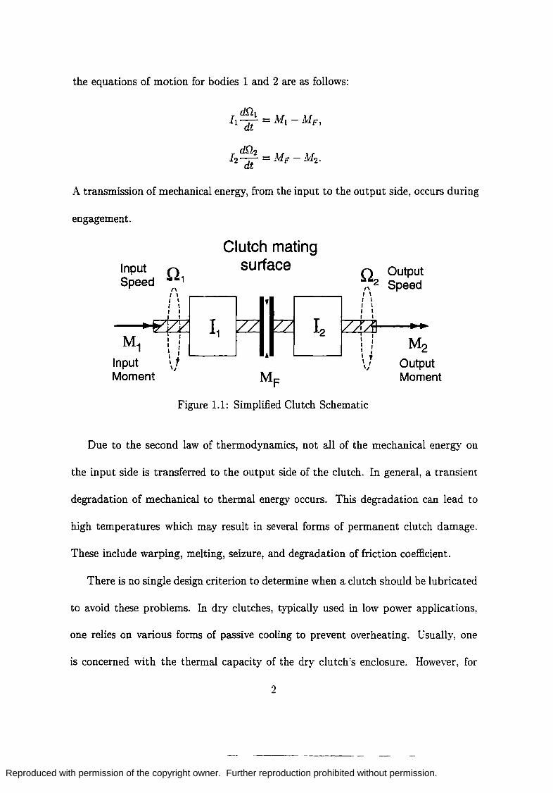
parts of a shaft or a shaft and a driving mechanism. Figure 1.1 shows a simplified
schematic of a clutch. A rotating input shaft with inertia, II, and angular velocity,
0 1 , engages a rotating output shaft with inertia, 12 , and angular velocity, O2 . In
some cases, O2 will initially be zero. A driving mechanism supplies an input moment.
kI1• In general, the driven side, or output side will have a load moment, A£2, which
will effect the engagement process. Friction is the physical mechanism through which
engagement occurs. If a frictional moment, }VIF , acts at the clutch mating surface,
1
Reproduced with permission of the copyright owner. Further reproduction prohibited without permission.
the equations of motion for bodies 1 and 2 are as follows:
A transmission of mechanical energy, from the input to the output side, occurs during
engagement.
Input Speed
M1 Input Moment
" , I , I , I , I
I
I I I I
I ' I ' I t \"
Clutch mating surface
, II Output ~~2 Speed , I , I , I , I I I
I I M , I 2 I I I I IJ Output
Moment
Figure 1.1: Simplified Clutch Schematic
Due to the second law of thermodynamics, not all of the mechanical energy on
the input side is transferred to the output side of the clutch. In general, a transient
degradation of mechanical to thermal energy occurs. This degradation can lead to
high temperatures which may result in several forms of permanent clutch damage.
These include warping, melting, seizure, and degradation of friction coefficient.
There is no single design criterion to determine when a clutch should be lubricated
to avoid these problems. In dry clutches, typically used in low power applications,
one relies on various forms of passive cooling to prevent overheating. Usually, one
is concerned with the thermal capacity of the dry clutch's enclosure. However, for
2
---- --

Reproduced with permission of the copyright owner. Further reproduction prohibited without permission.
Clutch mating Input 0 1
surface ~ Output
Speed Speed 1\ 1\ I \ 1\ I \ , I , I \ I , I , I , , I ,
11 M1
I , I I I I I M2 I I I I I I , I
Input \ t ' ' Output \1 Ii
Moment Cool oil in Hot oil out Moment
Figure 1.2: Simplified Clutch Schematic with Lubrication
high power applications, a different strategy is to actively cool the mating surfaces as
illustrated in Figure 1.2. A lubricant acts as a cooling medium by conveying thermal
energy generated between clutch plates. In general, the purpose of lubrication in
clutches is to cool frictional surfaces while maintaining desirable friction characteris-
tics. This strategy of active cooling and its effect on the frictional characteristics of
disk clutches will be modeled in this research.
1.2 Overview of Current Research
In order to investigate the thermal and frictional effects in rotating disk clutches.
three models have been developed. They are (1) a thermal model which, considering
only the plates, predicts clutch temperature distributions using a presumed friction
coefficient, (2) a fluid model which, considering only the lubricant, predicts a friction
coefficient using velocity, pressure, and temperature distributions, and (3) a conjugate
model which considers the domains encompassing both plates and fluid. The subject
of this dissertation is the conjugate model. Each model has benefits and shortcomings.
3
--------

Reproduced with permission of the copyright owner. Further reproduction prohibited without permission.
These will be discussed here.
To adequately discuss the thermal model, some preliminary comments regarding
clutch plates are given here. A disk clutch assembly is composed of friction plates
and separator plates. Friction plates, which tend to be associated with the input side
of a clutch, have three composite material regions as shown in Figure 1.3. The two
outer regions, or lining materials are referred to as the friction material. The inner
core region of the friction plate is referred to as the backing material. Unlike friction
plates, separator plates are made of a single homogeneous region and are usually
associated with the output side of a clutch.
The thermal model predicts a detailed temperature distribution in an assembly
of clutch plates without consideration of the fluid film. Figure 1.3 illustrates the
configuration for the thermal model. Here, 2Lb is the axial thickness of the backing
material, 2Ls is the axial thickness of the separator plate, and L f is the a.xial thickness
of the friction material lining on each side of the friction plates. The temperature
distribution can be obtained by solving the thermal energy equation. At the interfacial
boundaries of the clutch plates, continuity of temperature and heat flu..x is enforced.
Heat is generated at these interfaces using specified friction coefficients and pressure
distributions. At all other boundaries to the clutch, passive cooling is modeled by
specifying the ambient convection coefficients, hoo , and ambient temperatures, Too,
as shown in Figure 1.3. Further, the thermal model accounts for different thermal
properties in the three material regions: (1) the friction material, (2) the backing
material, and (3) the separator plate.

Reproduced with permission of the copyright owner. Further reproduction prohibited without permission.
z'
Passive Cooling
T Separator plate
Backing material •
Friction material
Heat Generated by Friction
M~n.-QJ
Figure 1.3: Thermal Model Schematic
In addition to predicting the temperature field, the thermal model predicts clutch
speed and torque. A shortcoming of this model is that a friction coefficient must be
specified a priori. This is considered a shortcoming because the coefficient of friction
is a contrived quantity which could, in principle, be determined from the physics of
clutch engagement. The thermal model is discussed in further detail by Quast and
Smith [47] and is not considered in detail in this dissertation.
The fluid model predicts a friction coefficient given the lubricant properties, clutch
operating conditions, and geometry. A steady state, incompressible flow field is found
in a cylindrical frame, (r, (), z), between a pair of rotating clutch plates. The cylindrical
5
-------

Reproduced with permission of the copyright owner. Further reproduction prohibited without permission.
Absolute Frame :11 e.. ----II~j I 01r : I • I
Zt"----t/ t" : ..--- h h(r.9.t) '--__ oJ Q _ lubricant
119
Lubrication Problem Domain
(a)
Rotating Frame j II e.. ----.;.j I I I I I I
Zt t / th(r.9) ''--IU-brl-ca-n-t ..... :
119 I .
Lubrication Problem Domain
(b)
Figure 1.4: Fluid Model Schematic
frame rotates with the clutch friction plates. In other words, velocities are reported
with respect to an observer rotating with the friction plates. Figure 1.4 illustrates the
fluid model. Here, Bo is the domain angle of periodicity, h is the local film thickness
which is assumed to be a known function of rand B, and ho is the minimum film
thickness. In Figure 1.4(a), the absolute frame is shown in which the angular velocity
of the friction plate is 0 1 and the angular velocity of the separator plate is O2 , The
rotating frame in which we will study the problem moves with the friction plates as
shown in Figure 1.4(b). Here, nd = n2 - n1 is the angular velocity of the separator
plate as viewed in the rotating frame. In the absolute frame, the film thickness is
considered a function of time. However, in the rotating frame the film thickness is
6

Reproduced with permission of the copyright owner. Further reproduction prohibited without permission.
independent of time. In addition, the transformation to the rotating frame gives rise
to additional terms, namely centripetal and Coriolis terms, in the governing equations.
In the lubricant, velocity, pressure, and temperature distributions are determined
which may be used to predict other clutch performance parameters including fric
tional moments, normal loads, friction coefficients, and radial volumetric flow rates.
However, a coupling between the thermal model and the fluid model is still required
because temperature continuity and heat flux continuity is enforced at the solid-fluid
interface.
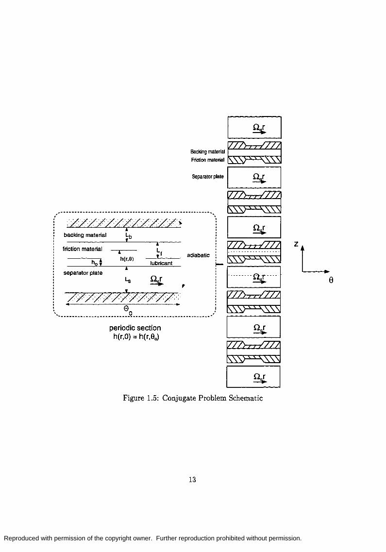
The conjugate model predicts both temperature distributions in the solid clutch
plate assembly and velocity, pressure, and temperature distributions in the lubricant.
A schematic of the model under consideration is shown in Figure 1.5. A lubrica
tion model is developed between two adjacent, rotating clutch plates. This model
is coupled to a model in the adjacent plates by requiring temperature and heat flux
continuity across the interfaces. As shown in Figure 1.5, a periodic section of a radi
ally grooved friction pair is considered. While periodic, the theory is developed using
an otherwise arbitrarily shaped film. Further, the domain of interest consists of a
friction plate and a separator plate separated by a lubricant film.
In the long time limit, a steady state solution is sought for the conjugate heat
transfer problem. In such a scenario, towards the middle of an assembly of clutch
plates, the temperature gradient is expected to vanish near the center of friction and
separator plates resulting in adiabatic conditions at the lubricant/solid interfaces.
Several results are given for this worst case scenario of clutch plate engagement.
7

Reproduced with permission of the copyright owner. Further reproduction prohibited without permission.
However, some discussion and results are presented for a more general problem which
considers the presence of passive cooling at the end of an assembly of clutch plates.
1.3 Utility of the Research
Analyzing clutch behavior often involves a variety of conflicting design criteria.
These devices are designed to deliver a certain amount of torque while experiencing
limited or no wear. \Vear tends to cause friction coefficient degradation resulting in
inconsistent clutch performance. Further, at the design stage, one should be wary
of large temperature rises which may result during clutch engagement. High tem
peratures decrease lubricant viscosity leading to a decrease in clutch frictional per
formance. Moreover, clutches are designed with the intention of meeting a certain
engagement schedule. That is, given a torque and a slip speed, a clutch is designed
to engage in a certain amount of time, typically under a second.
The reason that meeting these criteria is difficult is that the expectations men
tioned are not mutually exclusive. In other words, obtaining a desired torque level
within specified design constraints such as low temperature rises, scheduled engage
ment time, and other operating conditions may be physically impossible.
In order to meet these demanding e:x-pectations, a necessary first step to under
standing and ultimately optimizing clutch design is to have a valid model. The goals
of this dissertation are to (1) construct a model which can be used as a design tool,
and (2) to evaluate model results. These goals are discussed here.
Various lubrication theories may be adopted to construct this design tool. Some
8
---.-----

Reproduced with permission of the copyright owner. Further reproduction prohibited without permission.
background concerning these theories is given here. Hamrock [22} classifies the lubri
cation regimes as shown in Table 1.1. The thick and thin film regimes are considered
hydrodynamic. Here, the ratio of film thickness to surface roughness, A, is large
enough to neglect asperity contact, and the geometry may be considered smooth. In
the hydrodynamic regime, a continuum of lubricant fluid is recognizable. As the film
thickness gets smaller, the surface roughness becomes more significant, and asperities
begin to support the load. The mixed lubrication regime gets its name from the fact
that the load is supported by both asperities and the lubricant. Finally in the bound
ary lubrication regime, the load is supported by asperities and the lubricant's effects
are qualified using chemistry. For example, boundary lubricants form molecular films
on the solid surfaces which serve to protect the surfaces from high friction and wear.
It is known that the lowering of friction produced by a boundary lubricant is in di
rect proportion to its molecular weight, and therefore the length of the hydrocarbon
chain [30}. Thus, chemistry is employed to qualify the effect of boundary lubrication.
Here, the surface geometry and frictional conditions become too complex for a simple
continuum model.
Hydrodynamic lubrication theory starts from the perspective that the film size is
large enough such that existing continuum theories are valid. Typical mathematical
models use the Reynolds equation which may be derived from the more general Navier
Stokes equations in certain distinguished limits. However, assumptions built into the
derivation of the Reynolds equation are relaxed in this dissertation. In particular, the
assumption of constant viscosity across the film is investigated. In general, it is our
9

Reproduced with permission of the copyright owner. Further reproduction prohibited without permission.
Lubrication Range of Load
Regime Validity Supported By
Thick Film (hydrodynamic) lD<A<oo Lubricant
Thin Film (hydrodynamic) 3 < A < 10 Lubricant
Mixed I<A<3 Lubricant and Asperities
Boundary O<A<1 Asperities
Table 1.1: LUBRICATION REGIMES (A = su~~"b~~g~:~~ss)
intention to model this problem from first principles.
The first goal mentioned was to construct a model to be used as a design tool.
Properly constructed, such a design tool can be employed to save money, resources.
and time. Numerous experiments could be performed in different environments, with
different clutch plates, using different lubricants, while running at different operating
conditions. On the other hand, significant effort is required to create a complete
mathematical model. While a complete mathematical model is beyond the scope of
this dissertation, the number of experimental scenarios can be dramatically reduced
with simplified mathematical models.
The second goal, evaluating the model results, consists of (1) indicating trends.
(2) identifying deficiencies, and (3) proposing needs for future work. Expected or
unexpected results obtained from this model are indicated and questioned. Do the
parameters used as input predict a logical output? Can the results be used to model
10
---------

Reproduced with permission of the copyright owner. Further reproduction prohibited without permission.
actual clutch engagement? vVhat additional physics should be considered to improve
the model? These questions are addressed in the final chapter of this dissertation.
1.4 New Contributions
This dissertation contains many new contributions. Three major contributions
are allowing for a variable film shape, allowing for a variable viscosity, and coupling
the heat transfer problem to the fluid problem. The first two are discussed here.
Hydrodynamic lubrication theory has never been applied to lubricated disk clutches
with an arbitrary film shape. Fluid mechanics problems have been considered in radial
grooves [43, 44] and simplified models have been constructed for disk couplings [63].
Further, algebraic mappings which transform a complex domain into a manageable
domain are commonly found in computational fluid mechanics studies. Nevertheless,
these studies rarely consider arbitrary geometries. In other words, the geometry is
typically specified prior to solving the problem of interest. Allowing the film shape
to be defined arbitrarily enables virtually any groove pattern to be studied. Further-
more, macroscopic and microscopic deformations could be accommodated using this
theory.
Although viscosity variation is claimed in many lubrication studies, the fact is
that these models have a viscosity which does not vary in the axial direction. This is
not to say that numerical codes which claim to accommodate variable viscosity have
not been written.t However, classical derivations of the Reynolds equation assume a
tCFX5, for example, claims to accommodate variable properties. CFX5 is a thermofluids analyis code maintained by AEA Technology located in Pittsburgh, Pennsylvania.
11
Reproduced with permission of the copyright owner. Further reproduction prohibited without permission.
uniform viscosity across the film, and this assumption usually gets carried into the
model of interest. It is worth the effort to allow for viscosity variation in clutches
because drastic changes in viscosity result from a sensitive temperature relationship.
As will be shown, neglecting variable viscosity may result in significant errors in
several clutch performance predictions. Furthermore, allowing the viscosity to vary
across the film not only has potential in clutch studies, but may be generalized to a
larger set of lubrication problems.
12
Reproduced with permission of the copyright owner. Further reproduction prohibited without permission.
Backlngrna"''' ~ Friction material
"pa~to, pate I !¥ I
------------------------------------------------------ ~ -',
backing material
friction material
h 1 0' separator plate
1 h(r.e)
1 lubricant
n, --:"'/~ "T:""./::--r--. /:: -r-'/: ....,.-::/"7""".; ~ /.~0.1r-.:: /""'7"""'/: ~ ... /""7""" .. / . . --r-/: --r-.... :
. " .. "/0/"/>/", ._/" ... " .. .. .. e
adiabatic
,
• 0 ' ~------------------------------------.-----------.-----~
periodic section h(r,O) = h(r,8o)
I !¥ I
~ "'Iuu~uul
~ I !¥ I
~ I !¥ I
Figure 1.5: Conjugate Problem Schematic
13
e

Reproduced with permission of the copyright owner. Further reproduction prohibited without permission.
CHAPTER 2
LITERATURE REVIEW
This review of the relevant literature is divided into four sections: the first gives an
overview of clutch studies, the second reviews several devices which are mec!lanically
similar to disk clutches, the third discusses tribological issues pertinent in modeling
clutches, and the fourth focuses on several fluid mechanics and heat transfer problems
related to clutches. In the first section, the clutch studies overview considers both the
oretical and experimental work. The second section discusses studies concerned with
rim clutches, disk brakes, and disk couplings. The discussion on tribological issues
includes a discussion on lubricant properties and a discussion on surface topography.
Finally, the overview of heat transfer and fluid mechanics problems discusses axisym
metric rotating geometries including single and multiple disks in an infinite quiescent
fluid, hydrodynamic lidded annulus problems, and differentially heated cavities.
2.1 Clutch Studies
Several topics encountered in studying disk clutch engagement are evident in the
literature: comparing lubricant performance, friction coefficient degradation, wear of
friction surfaces, microscopic and macroscopic deformation, and the influence of ther
mal effects including convection, conduction, and thermoelastic deformation. The
fact that modeling clutches involves many disciplines has led authors to focus on par
ticular problems. However, several authors have constructed robust models capable
14
---------

Reproduced with permission of the copyright owner. Further reproduction prohibited without permission.
of predicting clutch performance under a variety of conditions. Theoretical models
and experimental investigations are discussed here.
2.1.1 Theoretical Models
Payvar [43, 44] has done extensive work in modeling fluid mechanics and heat
transfer in the radial grooves of a pair of clutch plates. In his earlier paper, he devel
ops a method to determine heat transfer coefficients in the grooves. In particular, he
assumes a Couette flow pattern in the oil film and couples this to a numerical solution
in the groove. He treats the film and recirculation zone in the groove as independent
thermal resistors which may be added in series to determine the overall heat trans
fer coefficient. His numerical results compare well with his experimental results. In
his later paper, Payvar gives a comparison between experimental techniques and a
numerical solution. He considers the steady incompressible Navier-Stokes equations
and a diffusing species concentration equation which is analogous to an energy equa
tion. By obtaining measurements for the net sublimated mass of naphthalene before
and after a certain time period, comparisons between the average Sherwood number
obtained numerically and experimentally were given. All in all, while he considers
many terms in the Navier-Stokes equations, he has a limited parameter space. In his
models, he neglects viscosity-temperature effects, assumes a flow solution adjacent to
the grooves of the friction plates, and insulates the friction plates to expedite a so
lution. Nevertheless, he predicts convection coefficients based on groove dimensions.
Reynolds number, and Nusselt number.
The conditions of clutch operation can have significant consequences on the lubri-
15

Reproduced with permission of the copyright owner. Further reproduction prohibited without permission.
cant. The sensitive viscosity-temperature relation should be considered in hydrody
namic models. Natsumeda and Miyoshi [381 develop a fairly elaborate clutch model
which takes viscosity-temperature effects into account. However, as suggested in the
previous chapter, this model does not account for viscosity variation across the film.
Nevertheless, they allow for clutch plate waviness, elastic deformation due to asperity
contact, and surface roughness using Patir and Cheng's model [411. Their model may
be considered a mixed lubrication problem. However, many questionable assump
tions are made in the formulation of the model. For example, asperity deformation is
assumed elastic which should be confirmed by computing a Greenwood-vVilliamson
plasticity index [301 or by some other rational method. Nevertheless, they make a
valuable contribution by computing the load carrying capacity using both asperity
contact and hydrodynamic lubricant pressure. Bardzimashvili and Yashvilli [3] de
scribe a method which accounts for not only the mixed regime of lubrication, but the
hydrodynamic and boundary regimes as well. However, results are not given. Their
model predicts multiple disk clutch torque and angular velocity using an interrelated
set of ordinary differential equations. They do not account for thermal effects.
Severe wear of clutch lining materials has motivated many studies, including Solt
[59] who attempts to optimize the load distributions using finite element methods.
He explains that non-uniform loadings, which induce deformation, lead to wear near
the location of maximum pressure. For known clutch plate dimensions, his results
suggest that there is an optimum location for the actuating force. Zagrodzki [691 de
velops a similar model which is generalized to account for thermoelastic effects. His
16
--------

Reproduced with permission of the copyright owner. Further reproduction prohibited without permission.
two-dimensional, time-dependent heat conduction model accounts for heat generation
and elastic deformation due to dry contact. Yevtushenko and Ivanyk [68] estimate
the surface temperatures and normal temperature displacements due to thermoelas
tic effects using a straightforward analytic model. They show that the change in
magnitude of contact area due to thermal distortion may be neglected.
2.1.2 Experimental Investigations
The choice of lubricant has Significant effects on the performance of disk clutches.
Ito, Fujimoto, Eguchi, and Yamamoto [32] experimentally determine clutch friction
coefficients under various conditions. In addition to varying the lubricant, their
studies include variable speed, loading, and friction plate porosity. Results indicate
marked difference in clutch performance. In particular, two oils were used: Dex
tron 2 automatic transmission fluid (ATF) and a paraffinic mineral oil which was
equivalent to the base oil of the ATF. For a range of sliding velocity varying from
0.01 to 1.0 ":' the ATF's friction coefficient remained fairly constant at 0.15 while
the paraffinic oil's friction coefficient approximately changed from 0.2 to 0.1. This
is significant because the ATF will provide a nearly constant torque level over this
speed range and the paraffinic oil's torque level could reduce by one half. Ichihashi
[31] discusses the increasing trend of equipping automobiles with ATF's as well as
developing improvements in ATF additives for improved clutch performance. Scott
and Suntiwattana [56] examine wear rates, lubricant temperature, and clutch torque
by varying the relative quantities of five different additives to the same base oil. Scott
and Suntiwattana report marginal differences in clutch friction coefficient and lock-up
17
---- --

Reproduced with permission of the copyright owner. Further reproduction prohibited without permission.
time with different additive concentration.
Viscosity-temperature effects are one of many effects which can be used to explain
degradation of clutch friction coefficients. Another effect is the presence of additives.
Inorganic additives added to the base oil chemically attack asperities yielding differ
ent friction properties of the mating surfaces. Still another effect is direct wear of
friction materials. Osani, Ikeda, and Kato [39] show that there is a distinct degree
of carbonization of paper-based facings beyond which the friction coefficient drops
off rapidly. Schulz [55] agrees that this gaseous form of wear plays a major role in
determining friction characteristics in a disk clutch.
2.2 Related Mechanical Devices
Takemuro and Niikuro [63] analyze viscous disk couplings which may be used in
limited slip differentials. Disk clutches and disk couplings have very similar geome
tries. Each may contain multiple disks which rotate for the purpose of transmitting
torque. However, disk couplings have separator rings which ensure a finite clearance
between adjacent plates. Takemuro and Niikruo develop a straightforward method to
determine torque, temperature rise, and dynamic response in the couplings. Viscosity
temperature effects and non-Newtonian effects are taken into account to model the
working fluid, silicone oil. However, an energy equation was not stated explicitly for
the lubricant. Rather, a numerical method which employed a lumped analysis was
used to obtain the temperature at disk interfacial locations. In other words, spatial
temperature gradients in the fluid were ignored.
18
-------

Reproduced with permission of the copyright owner. Further reproduction prohibited without permission.
vVhittle, Atkin, and Bullough [64] examine a rim clutch filled with an electrorhe
ological fluid. As in other clutch lubrication problems, the equations of motion are
analyzed under the assumption of small clearance. U nUke a disk clutch, the small
clearance in a rim clutch is the difference in radii.
Stebar, Davison, and Linden [60] examine the effects that various automatic trans
mission fluids have on the torque versus time curve for band clutch engagement. Their
experimental results indicated that the choice of lubricant can have dramatic effects
on shift smoothness, clutch capacity, energy absorption, lock-up torque, and engage
ment time.
2.3 Trihological Issues
Tribology is the science of the mechanisms of friction, lubrication, and wear of in
teracting surfaces that are in relative motion. Here, two pertinent aspects of tribology
are discussed: (1) rheology of mineral oils, and (2) surface topography.
2.3.1 Mineral Oil Rheology
This discussion of mineral oils is divided into four sections. First, a discussion of
mineral oils' chemistry is given. Second, the constitutive equation relating the stress
and strain rate tensors is discussed. Third, comments regarding property variations
are given. Fourth, a specific discussion of the viscosity-temperature relation is given.
Chemistry of a Mineral Oil
Hamrock [22] and Robertson [48, 49] give synopses of the chemistry of mineral
oils and why their chemistry is important from an engineering perspective. :\lineral
19

Reproduced with permission of the copyright owner. Further reproduction prohibited without permission.
oils are composed of paraffinic chains and naphthenic rings of hydrocarbons. Paraf
fins tend to weigh less, have less severe viscosity-temperature relations, and have
higher flash and fire points than naphthenes. N aphthenes have lower pour points
and produce less carbonaceous residue at extreme temperatures. These flash, fire,
and pour points, indicative of a mineral oil's temperature related classification, will
be discussed shortly. In lubrication applications, additives are used to improve the
friction properties of the base oil. Singh [58] discusses viscosity index improvers such
as oil soluble polymers which tend to decrease the viscosity's dependence on temper
ature depending on the base oil character, type of finishing procedure, and additive
concentration.
Stress-Strain Rate Relation
Mineral oils exhibit Newtonian behavior over a wide range of operating conditions.
N on-Newtonian effects come into play with very large strain rates and are usually
considered in the presence of additives such as oil soluble polymers. Roelands [50]
states that significant changes in the oil's viscosity occur at strain rates exceeding
107s-1. One should be concerned about the non-Newtonian character of the fluid
when the relative velocity is large and the film is thin. For the problem discussed in
this dissertation, typical strain rates are approximately 105 S-l which are significantly
below the point at which non-Newtonian effects occur .
. An extensive review of experimental and theoretical non-Newtonian fluid me
chanics is given by Wilkinson [65]. A more restricted study is given by Johnson
and Tevaarwerk [34] in which they analyze non-Newtonian effects in oil films using
20
-------

Reproduced with permission of the copyright owner. Further reproduction prohibited without permission.
experimental methods.
Property Variations
Pressure dependent viscosities are considered in non-conformal contact problems
such as modeling gears, cams, or bearings [23, 28]. A nonconformal contact occurs
when the bodies in question mate at a point under no load. For example: the contact
between two spheres is considered a nonconformal contact. Under such conditions, the
pressures become extremely high and viscosity variations become important. Specif
ically, Roelands [50] states that when the average pressure over the contact area
exceeds several thousand pounds per square inch, piezoviscous effects become impor
tant. On the macroscopic scale, a wet disk clutch has the geometry associated with
a nominally conformal contact problem, and pressure dependent viscosities may be
neglected. Typical clutch lubrication and actuation pressures rarely exceed two or
three hundred pounds per square inch.
For mineral oils, the specific heat and conductivity are relatively constant for
large changes in temperature [22, 50]. Compared to the changes associated with the
viscosity-temperature relation, these variations are extremely small.
For the range of pressures and temperatures considered in this lubrication prob
lem, mineral oils have a fairly constant density compared to the variation of viscosity
with temperature. Roelands [50] notes that the kinematic viscosity may be taken as a
good measure of the viscosity for mineral oils and other synthetic oils \vith nearly equal
densities. For a typical mineral oil, the variation in density with pressure becomes
significant (greater than one percent) at pressures exceeding 0.02 MPa. However. the
21

Reproduced with permission of the copyright owner. Further reproduction prohibited without permission.
variation of density with temperature is more sensitive. Density changes of nearly ten
percent occur from O°C to 160°C. Nevertheless, while it is unclear how seriously den
sity variations will effect clutch performance, these variations are small compared to
the relative change in viscosity for the same conditions and are consequently ignored.
Nevertheless, there is concern regarding incompressibility, at low pressures. If the
lubricant':; pressure falls below the vapor pressure, cavitation will occur. Batchelor
[4] notes the fundamental difference between a real liquid and an ideal incompress
ible fluid: negative pressures can be predicted in an ideal fluid, and a liquid cannot
support a large tension. Rather, Batchelor states that small pockets of gas appear in
the liquid which are responsible for cavity formation and supporting tension. Ham
rock [22] notes that mineral oils contain nearly ten percent entrained gases which
form cavities when the pressure falls below the saturation pressure. Further, he sum
marizes the traditional boundary conditions used in modeling converging/diverging
domains. Birkhoff and Hays [7] cite specific theorems regarding geometry and operat
ing conditions which necessarily lead to cavitation. Further, they developed a general
improvement over the Swift-Steiber boundary conditions [22] commonly employed
today. Coyne and Elrod [11] develop a rational method to apply boundary bound
ary conditions when cavitation is expected to occur in converging-diverging domains.
Surface tension effects are included in their analysis. Most importantly, they state
that the load carrying capacity does not vary appreciably no matter which boundary
conditions are used. In more general fluid mechanics problems, bubble formation is
treated using the full Navier-Stokes equations. Ryskin and Leal [51, 52, 53] develop
22
-------

Reproduced with permission of the copyright owner. Further reproduction prohibited without permission.
a numerical procedure for two-dimensional mapping of a liquid-solid interface with
unknown orientation.
Viscosity-Temperature Relation
For a wet disk clutch, the most quantitatively significant dependence of any phys-
ical property is that of the viscosity with temperature. Mineral oils are classified
according to their viscosity-temperature performance. For example, the familiar SAE
10-W30 designation is a Society of Automotive Engineers' approved classification of
a mineral oil.t The first number, 10, denotes the Saybolt Universal Viscosityt (SUV)
restrictions at 1300 F and at 2100 F. The alpha-numeric code, VV30, denotes the SlV
restrictions at 00 F.
Further temperature related classifications and restrictions on the viscosity of a
mineral oil exist. Several examples are mentioned here. The viscosity index (VI) is
a classification which measures the rate which a given mineral oil's viscosity changes
with an increase in temperature. A high viscosity index, indicative of small viscosity
variation with temperature, is considered desirable so that the lubricant film main-
tains stable frictional characteristics at high temperatures. The Flash Point is the
lowest temperature at which oil vapors appear. The Fire Point is the lowest temper-
ature at which a continuous combustion of oil occurs. In order to maintain the film.
the operating lubricant temperature should be safely below the Flash Point. The
Pour Point is the lowest temperature at which the oil will remain fluid enough to
tSince 1978, this method of classification has been accepted by the American Petroleum Institute (API) and the American Society for Testing and Materials (ASTM) [13].
tSee Hamrock [22] and/or Robertson [48, 49] for good discussions of the Saybolt Universal Viscosity.
23

Reproduced with permission of the copyright owner. Further reproduction prohibited without permission.
perform a required task. For example, an automotive application of the Pour Point
may be the lowest temperature at which oil will flow into the pump inlet of a crank
case. This is important in cold weather environments.
The fact that these loosely defined terms have become commonplace in practical
engineering applications has not helped to quantify a viscosity-temperature relation.
Exact numbers simply do not exist for every mineral oil. Rather, as mentioned above.
the viscosity of a mineral oil falls in a range given by the SUV restrictions.
Still, several attempts have been made to quantify the viscosity-temperature rela
tion for mineral oils. Hersey [24] cites nearly ten viscosity-temperature relationships.
Hamrock [22] cites three such relations. More recent authors, including Hussain [29]
have made attempts at modeling the viscosity-temperature relation. The viscosity
temperature relation used in this dissertation will be that of Walthers [18].
2.3.2 Surface Topography
Surface topography is a geometrical description of t.he surface of interest. In
modeling clutch plate engagement, both macroscopic and microscopic descriptions
are relevant. The macroscopic description refers to gross deformations or outstanding
geometric patterns while the microscopic description refers to the surface roughness
which is describable in a statistical sense.
In all previously mentioned deformation related studies, clutch plate deformation
occurs as a result of direct contact. Specifically, two mechanisms are responsible
for macroscopic clutch plate deformation: elastic and thermoelastic effects. Elas
to hydrodynamic lubrication (EHL) would likely not occur on the macroscopic scale
24
-------- ---- --

Reproduced with permission of the copyright owner. Further reproduction prohibited without permission.
because, as mentioned previously, the engagement of clutch plates is a nominally
conformal contact problem. Again, in a conformal contact problem, the lubricant
pressure will act over a greater area and not cause any significant deformation. In
fact, Hoglund and Jacobson [26] state that in an EHL contact the pressures are very
high (1 - 3 GPa). This is three orders of magnitude higher than typical clutch
actuation pressures, 2 Jy[ Pa.
EHL may be relevant on a microscopic scale. Certainly significant asperity de-
formation occurs as a result of direct contact between engaging clutch plates. This
has been modeled in several of the mentioned clutch studies. On a microscopic scale.
statistical descriptions seem to be the only rational method to incorporate surface
roughness in the models.
Hamrock [22] and Hutchings [30] give discussions on how to quantify surface rough-
ness. The most popular measure of surface roughness, (j, is the root mean square (rms)
of the height measured from the mean surface height:
1 rC 2
(j = c, 10 Z (8) ds.
Here, C, is the measured length of a simple trace and Z (s) is the local height computed
above and below the mean value at the s-location along the trace. The trace is usually
taken with a device known as a stylus profilometer [30].
One of the difficulties with using the above description of surface roughness is
that it only gives a two-dimensional sample of the entire three dimensional surface.
Sullivan, Poroshin, and Hooke [62] discuss the necessity of incorporating a three-
dimensional description of the surface roughness. Further, they discuss problems
-.- ------

Reproduced with permission of the copyright owner. Further reproduction prohibited without permission.
encountered in differentiating between elastic and plastic deformation of asperities.
Three-dimensional surface roughness effects have been included in several lubrication
studies [66, 70]. In these studies, Patir and Cheng's [41, 42] work on developing an
average Reynolds equation to obtain the pressure was used. In particular, Patir and
Cheng use an equation which takes surface roughness and non-isotropic asperity ef
fects into account. Specifically, given the gross film thickness and limited information
about the microscopic description of the surface, they introduce what they label flow
rate factors to predict the lubricant pressure in separate lubrication studies.
2.4 Related Fluid Mechanics and Heat Transfer Problems
The fluid mechanics and heat transfer problems discussed in this section are ex
amples of axisymmetric flow adjacent to solid rotating disks. There is a wealth of
basic studies of such flows, a few of which are mentioned here.
Batchelor [5] has considered the steady axisymmetric flow between two infinite
rotating disks. He reduced the governing equations using an assumed similarity so
lution. His results may be used to obtain information locally to a set of finite disks.
Millsaps and Pohlhausen [36] generalized Batchelor's similarity solution to include
heat transfer. Stewartson [61] provided experimental evidence supporting Batche
lor's predicted streamlines when the disks rotate in the same direction. Lance and
Rogers [35] solved the hydrodynamic problem numerically. They present results for
the two dimensionless parameters: the ratio of the angular velocities of the disks and
the Reynolds number. Boundary layers in single disk solutions using the similarity
26
-------

Reproduced with permission of the copyright owner. Further reproduction prohibited without permission.
solution are discussed extensively by Schlichting [54]. Pearson [45] generalized the
previous hydrodynamic theory to include time-dependent terms in the Navier-Stokes
equations. In particular, he obtained numerical results using a generalized similarity
transformation with either one or two impulsively started infinite disks. Unlike pre
viously mentioned authors, Pearson's problem involves partial differential equations
with time and axial position as independent variables.
Recent improvement in computer hardware and numerical methods has enabled
the systematic computation of solutions to larger sets of partial differential equations.
Evans and Grief [15] consider flow and heat transfer around a rotating disk chemical
vapor deposition reactor. Compressibility and buoyancy are taken into account. Here,
a single disk is centered in a cylindrical tube. The spin axis of the cylinder and the
gravity vector are coaxial. Buoyancy effects in differentially heated rotating vertical
cavities are discussed by Barcilon and Pedlosky [1, 2] and Homsy and Hudson [27].
Their work included obtaining physical solutions by formally linearizing the equations
of motion in the limits of small and large Eckman number. Chew [9] and Guo and
Zhang [20] present numerical results for these rotating lidded cylinders.
Lidded annulus problems are reviewed extensively by Oi Prima and Swinney [12]
within the context of studying instabilities in Taylor flow. Experimental results show
ing Taylor vortices in lidded cylinders are given by Cole [10]. Numerical results for
chaotic flow in a lidded annulus are presented by Hadid [21].
27
- -- - -----

Reproduced with permission of the copyright owner. Further reproduction prohibited without permission.
CHAPTER 3
MATHEMATICAL MODEL
This chapter gives the mathematical statement of the problem investigated in this
research. In the first section, the domain and physical variables are defined. In the
second section, the mass, momentum, and energy equations are listed, and under
lying assumptions pertinent to disk clutch lubrication are discussed. In the third
section, constitutive equations are stated. In the fourth section, boundary conditions
are stated. In the fifth section, the equations are non-dimension ali zed and written
in terms of 0 (1) dimensionless variables and appropriate dimensionless quantities.
Further, the equations are simplified by examining the order of magnitude of the
dimensionless parameters. In the sixth section, the complete statement of the prob
lem is given. The seventh section introduces the algebraic coordinate transformation
used to solve the governing equations in a computational domain. In the eighth sec
tion, pertinent clutch performance parameters are defined in terms of the dependent
variables.
3.1 Domain and Variable Definitions
The lubrication problem is illustrated in Figure 3.1. Let r, 8, and z denote the
radial, angular, and axial Eulerian cylindrical coordinates which rotate with angular
velocity 0 1 , coincident with the clutch friction plates. The separator plate angular
velocity, as viewed in the rotating frame, is rl d • The physical domain for the lubrica-
28
---.-----

Reproduced with permission of the copyright owner. Further reproduction prohibited without permission.
Coordinate system (r.9.z) rotates with friction plate
land
Friction plate stationary in rotating coordinate system
!lctr MOving separator plate
in rotating coordinate system
Lubrication Problem Domain
Problem Domain
Figure 3.1: Lubrication Problem Domain
tion problem as indicated in Figure 3.1 is defined by F4 :s; r :s; Ro , 0 :::; 0 :s; Bo, and
a :s; z :s; h (r, 0). Here, I4. and Ro are inner and outer clutch radii, 00 is the domain
angle of periodicity, and h is the local film thickness. The domain angle of periodicity
is the minimum angle required to replicate the entire film thickness. It is always
an integral fraction of 211". The film thickness, h, is a known periodic but otherwise
arbitrary function of rand O. That is, h (r, 0) = h (r, ( 0 ) = h (r, nOo), where n is
any integer. The radial channels shown in Figure 3.1 are referred to as grooves. The
29
Reproduced with permission of the copyright owner. Further reproduction prohibited without permission.
adjacent portions to the grooves are referred to as lands. Thus, the domain shown in
Figure 3.1 contains a groove and two half lands.
The general lubrication problem is then to determine the radial velocity, V r , the
angular velocity, vs, the axial velocity, vz , the pressure, p, and temperature, T, of
the fluid as functions of position and time. These quantities, with the exception of
vs, are invariant when referred to an absolute frame. The absolute angular velocity
is Vs + n1r. The radial flow of lubricant into the domain is affected by a specified
pressure difference. The radial inlet temperature of the lubricant is controlled with
an external cooling system.
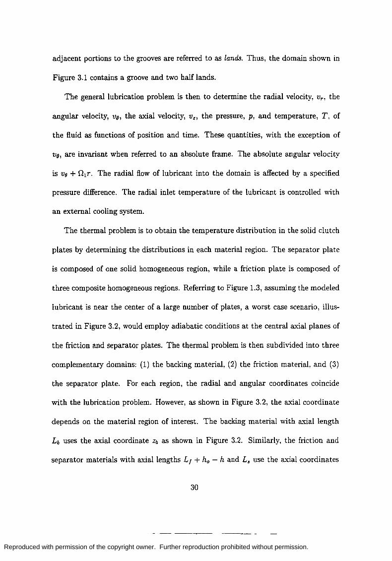
The thermal problem is to obtain the temperature distribution in the solid clutch
plates by determining the distributions in each material region. The separator plate
is composed of one solid homogeneous region, while a friction plate is composed of
three composite homogeneous regions. Referring to Figure 1.3, assuming the modeled
lubricant is near the center of a large number of plates, a worst case scenario, illus
trated in Figure 3.2, would employ adiabatic conditions at the central axial planes of
the friction and separator plates. The thermal problem is then subdivided into three
complementary domains: (1) the backing material, (2) the friction material, and (3)
the separator plate. For each region, the radial and angular coordinates coincide
with the lubrication problem. However, as shown in Figure 3.2, the axial coordinate
depends on the material region of interest. The backing material with a.xial length
Lb uses the axial coordinate Zb as shown in Figure 3.2. Similarly, the friction and
separator materials with a.xial lengths L f + ho - h and La use the axial coordinates
30

Reproduced with permission of the copyright owner. Further reproduction prohibited without permission.
z/ and zs, respectively.
Symmetric Adiabatic Condtion
, ,
Backing Material Thermal Problem
Domain
Friction Material Thermal Problem
Domain
i-------------------------------f----i , , : : Separator Plate
zst' Separator Plate r:-The~~~~Oblem
-----777777777777777)?7) Symmetric Adiabatic Condtion
Figure 3.2: Thermal Problem Domain
3.2 Conservation Principles
To start, we adopt the incompressible Navier-Stokes equations to model the lu-
bricant behavior. "We assume the fluid is continuous and sufficiently thick to neglect
surface roughness effects. Body forces are neglected.
The condition of incompressibility requires the continuity equation to be of the
following form:
1 8 1 avo 8vz -- (rvr ) + -- + - = o_ r 8r r ao 8z
(3.1)
The momenta equations are written in a frame moving with the constant friction
plate angular velocity, fh:
[avr aVr V8 8vr 8vr 1 ( (") 2] P -+Vr-+--+Vz---V8+ H l r ) at aT r 80 8 z r
= _ 8p +!~ (r7rr ) +! ar8r + 87zr _ 788 ,
8r r 8r r 80 8 z r
(3.2)
31
--------

Reproduced with permission of the copyright owner. Further reproduction prohibited without permission.
[avo avo Vo avo avo vrvO 2r2 ]
p at + Vr ar + -;: a8 + v: az + -r- + 1 Vr (3.3)
= _~ ap + ~~ (rTrO) + ~ aTOO + aT:o + TrO, r 88 r 8r r 88 8z r
[8V: 8v: Vo 8v: 8V:] _ _ 8p ~~ ( ) ~ 8To: 8T:: (3.4)
P at + Vr 8r + r 88 + Vz 8z - 8z + r 8r rTrz + r 88 + 8z .
The lubricant energy equation, written to account for incompressibility, is as follows:
(3.5)
In Equations {3.2} through (3.5), Trr , TOO, Tzz , TrO = TOr, Trz = T:r, and Toz = T:O are
the components of the symmetric stress tensor, qT' qo, and qz are the components of
the heat flux vector, e is the internal energy per unit mass, and p is the density.
The governing equation used to predict the temperature distribution in each ma-
terial region of the solid clutch plates is the thermal energy equation. In the rotating
frame, the thermal energy equations for the material regions in the friction plates is
as follows:
(3.6)
(3.7)
Also in this frame, the thermal energy equation for the separator plates is as follows:
(3.8)
In Equations (3.6-3.8), the subscripts j, b, and s denote friction, backing, and sepa-
rator material regions.
32
-~--------

Reproduced with permission of the copyright owner. Further reproduction prohibited without permission.
3.3 Constitutive Equations
The modeled lubricant is considered to be a Newtonian thermoviscous Stokesian
fluid [14]. The components of the stress tensor in cylindrical coordinates are defined
as follows:
Trr = 2JL ~~, TrO = JL [r! (~) + ~ ~~ 1 '
TOO = 2: [~~ + Vr 1 ' Toz = JL [~~ + ~ ~~z 1 ' (3.9)
In Equation (3.9), JL is the viscosity. The components of the heat flux vector in the
fluid are defined as follows:
aT qz = -k-. az (3.10)
Similarly, using Fourier's law in the material regions of the clutch plates, the compo-
nents of the heat flux vectors are defined as follows: aT kfaT 8T
qrf = -kf ar ' qOf = --;: ao' qzf = -kf azf
'
aT kb8T &T qrb = -kb ar ' Qob = --;:- 80 ' qzb = -kb 8z
b' (3.11)
aT ks 8T 8T qrs = -ks ar ' qos = --;:- 80' qzs = -ks 8z
s .
In Equations (3.10) and (3.11), k, kf' kb, and ks are the thermal conductivities for
the lubricant, friction material, backing material, and separator material respectively.
For the lubricant, the internal energy per unit mass is related to the temperature by
the following caloric equation of state:
e = cT. (3.12)
Likewise, the internal energy per unit mass in the clutch plates is defined as
(3.13)
33

Reproduced with permission of the copyright owner. Further reproduction prohibited without permission.
for the friction, backing, and separator materials respectively. In Equations (3.12)
and (3.13), C, cI, Cb, and Cs are the specific heats for the lubricant, friction material,
backing material, and separator material respectively.
SAE m A B Trel Prel
number x 10-11 x107 X 104
(Km) (~n (K) (~n
SAE 10 4.6384 5.8352 4294.1 300 712.1
SAE 20 4.5268 3.4057 2596.4 300 1113.2
SAE 30 4.3354 1.2779 5138.3 300 1968.8
SAE 40 4.4733 3.0758 -2209.4 300 3367.2
SAE 50 4.0416 .28723 1497.9 300 5805.2
SAE 60 3.9152 .14758 -3837.2 300 8390.4
SAE 70 3.8165 .08901 455.9 300 12420.0
Table 3.1: RESULTS FROM FITTING SHIGLEY'S DATA INTO \JVALTHERS'S EQUATION
The viscosity-temperature relation used in this dissertation is based on \Valther's
equation [18]:
This correlation has two noteworthy shortcomings. First, the kinematic viscosity can
not be measured experimentally. Therefore, there is an implicit assumption in this
equation that the viscosity depends on the density, 1/ = ;. However, the density is a
34
-------

Reproduced with permission of the copyright owner. Further reproduction prohibited without permission.
"E
'-
1.000
UI 0.100 I
z
~ 'iii o Iii 0.010 :>
Viscosit vs. Temperature
0.00 1 '--_~ ____ ~--'-~~_-'--' __ --L-. __ "'--
300 320 340 360 380 400 T, Temperature, (K)
Figure 3.3: Viscosity-Temperature Relation for Seven SAE Oils
thermodynamic property, the viscosity is a transport property, and there is generally
no correlation between them. Second, the dimensions on this equation are ambiguous.
It is assumed that the parameters A and BI have units of Km and ~2 respectively.
To avoid these problems, we adopt a hybrid of Walther's viscosity-temperature
relation,
10 (J.1. + B ) _ A (_1 __ 1 ) gIO J.1.reJ + B - Tm Tr~J '
(3.14)
which contains five parameters: m, A., B, TreJ and J.1.reJ. Here, J.1. is the viscosity at
temperature T. Equation (3.14) may be rewritten in the follmving form:
(3.15)
Here, J.1. is the viscosity at temperature T. The parameters were determined using
Shigley's [57] viscosity-temperature data for seven SAE oils. These are shown in Table
3.1. Viscosity-temperature plots are shown in Figure 3.3.
35
------ --------

Reproduced with permission of the copyright owner. Further reproduction prohibited without permission.
3.4 Initial and Boundary Conditions
Initial and boundary conditions for the general physical problem are given here.
First, initial conditions are given. Second, boundary conditions are given.
The following generalized initial conditions are given for the lubricant velocity and
temperature fields:
at t = 0 : vr = vro (r, (), z) , Vo = V80 (r, (), z) , Vz = VzO (r, (), z) , (3.16)
and T=To(r,(),z).
Similarly, generalized initial conditions are given for the temperature fields within the
material regions of the clutch plates:
att=O: T=To/(r,(),z/) for friction material,
for backing material, (3.17)
T = Tos (r, (), zs) for separator material.
It is further noted here that all bounding geometry and constraints are independent
of time. For example, the relative angular velocity of the separator plate, Od, is taken
as constant.
The classic no-slip condition is enforced on the clutch plate surfaces.
on z = 0: Vr = Vz = 0 (3.18)
on z = h (r, ()) : Vr = Vo = Vz = 0
Here, the only nonhomogeneous condition relates the angular component of velocity,
as viewed in the rotating frame, to the relative slip speed of the clutch.
The pressure is subjected to the following boundary conditions:
P (~, ()) = Pi, P (Ro, ()) = Po,
8p (r, 0) 8p (r, ()o) -8() 8()
(3.19) p (r, 0) = p (r, ()o),
36
- ~--- ----

Reproduced with permission of the copyright owner. Further reproduction prohibited without permission.
The pressure is prescribed at the inner and outer radii. The periodic conditions on
pressure are to be expected from the geometry.
In the fluid, the inlet radial temperature, To, is prescribed. Further, a periodic
condition on temperature is prescribed:
T (~, 0, z) = To, T (r, 0, z) = T (r, 00 , z) . (3.20)
The additional conditions for the temperature distribution couple the thermal and
fluid problems. vVe require temperature and heat fltL"{ continuity at all axial interfaces:
TI =TI ' zb=Lb Z/=O
TI -TI zf=L/+ho-h - z=h'
T! =T!. z,,=L. Z=O
aT! aT! - =- =0 8zb Zb=O 8zs Za=O '
81'1 aTl kb- =kf- , 8Zb zb=Lb 8zf Z/=O
(3.21)
aTl aTl ks - =k-, 8zs za=La 8z z=o
ki'V fT· nfl = -k"VT . n! . z/=L/+ho-h z=h
Here, nf and n are unit outward normals to the friction and lubricant's surfaces at
their common interface. Using the following relationships,
"VT = [ fr
187' T 80
1 ]
T 1 18h -r============== r 80 ( )2 ( )2 ' a;. + ~~~ +1
n = [ _ '!!:. _1 8h 1] T 1 ur r80 2 2'
(a;.) + U~~) + 1
the last of these conditions, given in Equation (3.21), may be simplified to the fol-
lowing equation:
[8h aT 1 8h aT] I aT I aT ! (kf-k) --+--- +k- +kf- =0 8r 8r r2 80 80 z=h 8z z=h 8zf z/=L/+ho-h .
37
- - - -----

Reproduced with permission of the copyright owner. Further reproduction prohibited without permission.
3.5 N on-Dimensionalization
The governing equations are non-dimensionalized in order to investigate the rel-
ative order of magnitude of the terms involved. The choice of scaling and typical
values of dimensionless parameters will be discussed in this section.
3.5.1 Choice of Scaling
First, the nondimensional independent spatial variables are defined as follows:
r r.= -,
E4 e. = e, z
z .. =-. ho
(3.22)
The radius, r, was scaled by the inner clutch radius, E4, and the axial coordinate,
z, was scaled by the minimum film thickness, ho• Again, the film thickness, h, is in
general a function of the radial coordinate, r, and the angular coordinate, e.
Second, the components of velocity were scaled as follows:
.. Vr
Vr = nl~' • Vo
Vo = nl~' • Vz
Vz = nlho· (3.23)
These scalings are chosen such that all terms in the continuity equation are given
equal significance. The angular component of velocity is scaled by the friction plate
absolute velocity, or the input driving velocity of the clutch.
Third, the viscosity and temperature were non-dimensionalized. Again, the lubri-
cant viscosity depends on temperature, /-L = /-L (T). Assuming the lubricant's charac-
teristic temperature is the radial inlet temperature, To, the characteristic viscosity is
/-Lo = /-L (To)· The viscosity and temperature were scaled as follows:
/-L /-L. = -, /-Lo
T T. = To. (3.24)
38

Reproduced with permission of the copyright owner. Further reproduction prohibited without permission.
Fourth, a dimensionless pressure was defined. Very large changes in pressure are
expected to occur in small clearances where relative velocities exist. This premise of
lubrication theory has motivated a widely accepted scaling of pressure [18, 22, 40]:
(3.25)
Here, the characteristic pressure, 1'o~!Rr, may be justified. If the clearance to radius o
ratio is smail, pressures are expected to be high. Increases in the angular speed and/or
viscosity are expected to increase the pressure. From Equation (3.19), the pressure,
Pi, is the uniform pressure at the inner radius of the clutch. At T = Ro, the pressure
is specified as P = Po, or P* = p~ in dimensionless terms.
Fifth, the time, t, was nondimensionalized. We assume that the appropriate
time scale may be found by considering the rate of change of the no-slip boundary
condition at the clutch surface. Here, we temporarily relax the previous statement
that the boundary constraints are independent of time. A simple equation which
relates the clutch frictional moment to the relative angular acceleration of the clutch
is as follows:
(3.26)
In Equation (3.26), load torques, T2, and the term ~~ in the (}z-stress component
have been neglected. Using the above dimensionless definitions and letting r2. de-
note the ratio of relative speed to input speed, r2. = ~, we can non-dimensionalize
Equation (3.26) as follows:
dr2. lRo 2 aVe -d = 27rT*/J·-a dT*,
t* 1 z* (3.27)
39

Reproduced with permission of the copyright owner. Further reproduction prohibited without permission.
where,
J.LoR{ t. = -h J. t.
o 2 {3.28}
Here, R. = t is the ratio of outer to inner clutch radii. It is clear that increasing the
viscosity will increase the torque delivered and decrease the time in which significant
changes occur in the relative slip speed. Further, increasing the film size or output
inertia would increase the time in which changes in the clutch slip speed occur.
Sixth, the dimensionless axial coordinates for the solid clutch plates were defined
as follows:
{3.29}
The notation used in Equation (3.29) corresponds to Figure 3.2. The corresponding
radial and angular scaling in the solid material regions is defined in Equation {3.22}.
3.5.2 Dimensionless Equations
The result of substituting the above dimensionless variable definitions, Equations
(3.22-3.25), (3.28), and (3.29), and the constitutive equations, (3.9-3.13), into the
governing equations, (3.1-3.8), the viscosity-temperature equation, (3.15), and the
initial and boundary conditions, (3.16-3.21), is shown below:
1 8 .. 1 avo av; --8 (r .. vr ) + -afJ + -a = 0, r .. r.. r.... z.
I av; R [ .. av; v; av; .. av; 1 ( .. )] ap. R-+f e v -+--+v --- vo+r =-at.. r ar.. r. ao.. z az.. r. .. ar.
2f2 a ( av.) f2 a [ ( a (V") 1 av .. )] r 0 r + -- J.L r - + -- J.L r - - +--r. ar.. ... ar.. r .. ao. • .. ar. r. r. ao .. a [ (2av; av;)] 2J.L .. f
2 ( 1 avo V;) +- J.L f -+- --- --+-az. • ar. az.. r. r .. ao.. r. '
40
-------
(3.30)
(3.31)

Reproduced with permission of the copyright owner. Further reproduction prohibited without permission.
I av; R [.av; v; av; .av; v; v; 2 .]_ 1 ap. Rat +€ e Vr-a +-afJ +Vz -a +--+ Vr - --afJ • r. r.. z. r. r. • €2 a [ (a (V· ) 1 av.)] 2 8 r + -- J.L r r - - +--r; ar. •• • ar. r. r. afJ. 2€2 a [ (1 av· v.)] a [ (av. €2 av.)] (J r 8 z +-- J.L --+- +- /-L -+--r. afJ. • r. afJ. r. aZ." aZ. r. afJ. '
21 av; 3R [.av; VB av; • av;] _ _ ap. € Rat + € e Vr a + afJ + Vz a - a .. r. r.. z. z.
1 a [ (av. av.)] €2 a [ (av. €2 av.)] 4 z 2 r (J z + -- fJ r € - + € - + -- /-L - + --r. ar. •• ar. az. r. afJ. .. az. r. afJ. 2 a [ av;] + 2€ az. /-L. az. '
IRGrffI'. G [.ffI'. v;ffI'. .ffI'.] -R at +€ r vr-a +-afJ +vz -a e. r. r... z.
€3 a ( aT. ) €3 a2T. a2T. = T. ar. T. ar. + r; ae; + € a z;
2 3 B [(av:)2 (1 av; V:)2 (av:) 2] + € TJ.L. - + -- + - + -ar. r. afJ. r. az.
B [ 3 ( 1 av; v; av; ) 2 (~ av; 1 av; ) 2 + rfJ. € -- - - + - + €2 - + €2-
r. afJ. r. ar. ar. az.
+ €2-+--( 1 av; €~ av;) 2]
az. r. afJ. '
I RPr ffI'. €2 a ( aT. ) €2 a2T. 1 a2T. aj at. = r. ar. r. ar. + r; afJ; + Lj2 azj2 '
I RPr aT. €2 a ( aT. ) €2 a2T. 1 a2T. --;;; at. = r. ar. r. ar. + r; afJ; + L'b2 az;2 '
IRPr ffI'. Grn. aT. €2 a ( aT.) €2 a2T. 1 a2T. ~ at. +~ afJ. = r. ar. r. ar. + T; afJ; + L:2 az;2'
_ (Ki + 1) exp [Ki (~ - K; m)] - 1
fJ. - (Ki + 1) exp [K2 (1 - Ki m )] - 1
at t. = 0 : v; = v;o (r., fJ., z.) , Vo = voo (r., fJ., z.) ,
and v; = v;o (r., fJ., z.) , T. = T; (r., fJ., z.) ,
·u
(3.32)
(3.33)
(3.34)
(3.35 )
(3.36)
(3.37)
(3.38)
(3.39)

Reproduced with permission of the copyright owner. Further reproduction prohibited without permission.
at t. = 0 : T. = T;f (r.,B.,zi) for friction material,
for backing material, (3.40)
for separator material,
on z. = 0 : v; = O.r., (3.41)
on z. = h. (r.,B.) : v; = v; = v; = 0,
p. (1, B.) = 0, p. (R., B.) = p~,
8p. ( ) 8p. ) 8B. r., ° = 8B. (r.: Bo : p(r.,O) =p(r.,Bo),
(3.42)
T. (1, B., z.) = 1, T. (r., 0, z.) = T. (r., Bo, z.) , (3.43)
T.I =T·I ' zb=l zi=o T.I = T·I ' zi=Li+1-h. z.=h.
I I aT. I aT. I T. = T. , - = - = 0, z;=l z.=o 8zb zi=O 8z; z;=o
kbLj aT. I aT. I k; aT. I 81'.1 kjLi, 8zb Zb=l = 8zj zi=o' L: 8z; z;=l = 8z. z.=O'
(3.44)
2 (k. 1) [8h. aT. 1 8h. aT.] I or. I € f- --+2-- +-
8r. 8r. r. 8B. 8B. z.=h. 8z. z.=h.
+ kj or. I = 0" Lj 8zj zi=Li+1-h.
Here, € = l£ is the ratio of film thickness to inner radius, Re = pnlRjho is the .... flo
Reynolds number, IR = P~ho is the ratio of fluid inertia to output clutch inertia.
Gr = Pcn:h~ is the Graetz number, Br = /lo~;oRr is the Brinkman number, v;o = n':r~i'
V • - ~ v· -...!!;.JL rr. - Tn. rr. - fu rr. -.Thl!. and rr. - ThL are the l"nl"tl"al /JO - nlR;' zO - nlho ' .Lo - To' .LOf - To' .LOb - To' .LOs - To
dimensionless velocity and temperature profiles, O. = ~ is the ratio of relative speed
to input speed, Pr = ¥ is the Prandtl number, Ki = /lSI, Ki = A ir:..LO , and o
K; = T.To are dimensionless parameters found in the viscosity-temperature equation, ref
-!2
---- --
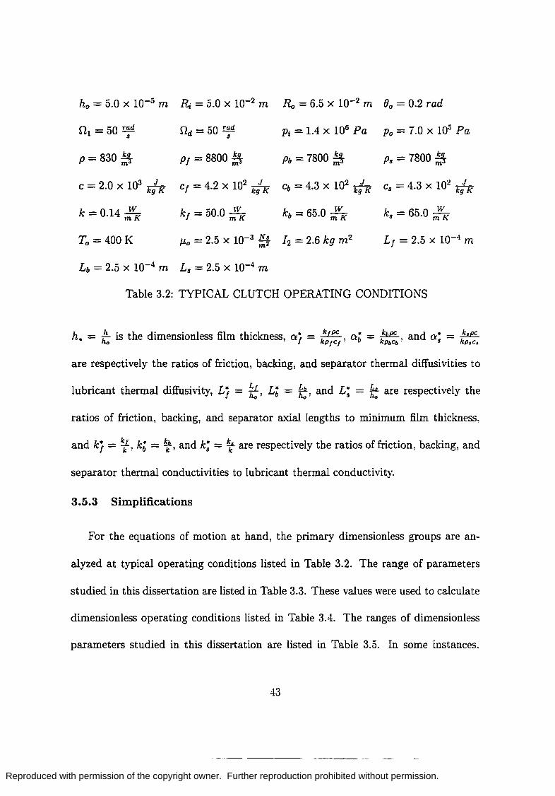
Reproduced with permission of the copyright owner. Further reproduction prohibited without permission.
ho = 5.0 X 10⁻⁵ m ~ = 5.0 X 10⁻² m Ro = 6.5 X 10⁻² m eo = 0.2 rad
0 1 = 50 Tad s Od=50 ~ s Pi = 1.4 X 10⁶ Pa Po = 7.0 X 10⁵ Pa
P = 830 ~ PI = 8800 ~ Pb = 7800 ~ Ps = 7800 ~
c = 2.0 X 10³ k: K CI = 4.2 X 10²
k:K Cb = 4.3 X 10² k: K
2 J Cs = 4.3 X 10 kg K
k = 0.14 mWK kl = 50.0 ~VK kb = 65.0 mWK ks = 65.0 ~VK
To = 400 K J.Lo = 2.5 X 10⁻³ ~~ [2 = 2.6 kg m 2 L, = 2.5 X 10⁻⁴ m
Lb = 2.5 X 10⁻⁴ m Ls = 2.5 X 10⁻⁴ m
Table 3.2: TYPICAL CLUTCH OPERATING CONDITIONS
h.. = hho is the dimensionless film thickness, Q,* = kkp',PcC" Q* = ~ and a* = ~ b kPbCb' 5 kp.c.
are respectively the ratios of friction, backing, and separator thermal diffusivities to
lubricant thermal diffusivity, Lj = ~, Lb = ~, and L; = t are respectively the
ratios of friction, backing, and separator axial lengths to minimum film thickness,
and kj = '¥-' k; = ~, and k; = ~ are respectively the ratios of friction, backing, and
separator thermal conductivities to lubricant thermal conductivity.
3.5.3 Simplifications
For the equations of motion at hand, the primary dimensionless groups are an-
alyzed at typical operating conditions listed in Table 3.2. The range of parameters
studied in this dissertation are listed in Table 3.3. These values were used to calculate
dimensionless operating conditions listed in Table 3.4. The ranges of dimensionless
parameters studied in this dissertation are listed in Table 3.5. In some instances,
43

Reproduced with permission of the copyright owner. Further reproduction prohibited without permission.
3 X 10⁻⁶ m $ ho $ 2.0 X 10⁻⁴ m 50 rad < n < 200 rad s - d - s
0.5 MPa $ Po ~ 2.0 MPa 300 K ~ To ::; 500 K
1.0 X 10⁻³ Ns < II < 7.0 X 10⁻² Ns m2 - t-o - m2
Table 3.3: RANGE OF PARAMETERS STUDIED
€ = ~ = 1.0 X 10⁻³
Gr = pcfl:h~ = 1.5
Pr= ¥ =36
a* = ..&e!:.. = 230 s kp.c.
Kt = &. = 0.33 lJo
Re = pOl EYho = 42 lJo
Br = lJo~joRr = 2.8 x 10⁻⁴
L* - !:L - 5 ,- ho -
R -&-13 *-Ri- .
K* -.& -11 2 - T:;' - •
IR = PRLho = 1.0 X 10⁻⁷
n -&-1 H* - 01 -
L* - f.ll. - :; b - ho - V
P* - (po-pilh~ - -5 6 o - lJoOlRr - •
Kj = &. = -0.15 lJo
Table 3.4: TYPICAL CLUTCH DIMENSIONLESS PARAMETERS
6 X 10⁻⁵ < € = fuz. < 4.0 X 10⁻³ - Ri -
9 X 10⁻⁵ ::; Br = lJo~foR; ::; 0.16
5 x 10⁻³ < Gr = pcOlh; < 105 - k-
Table 3.5: RANGE OF DIMENSIONLESS PARAMETERS STUDIED
44
---------

Reproduced with permission of the copyright owner. Further reproduction prohibited without permission.
a best guess is made for the operating conditions. The radii, ~ and Ro, and axial
lengths, Lb, Ls , and L" are based on a Clark 18000 forward first clutch. The material
and lubricant properties are based on steel for the backing and separator materials,
commercial bronze for the friction material, and SAE 10 for the lubricant. It is noted
that the operating parameters could significantly change the Brinkman and Graetz
numbers via the film size, input speed, and viscosity-temperature relation. Further
discussion on these parameter ranges is given shortly.
In view of the dimensionless numbers predicted, the following arguments are made
to simplify the governing equations:
1. All dimensionless variables, t., T., 0., Z., v;, ve, v;, p., T., and J.L., are 0 (1).
2. The ratio of fluid to solid inertia, I R , is negligible.
3. The solid to fluid thermal diffusivity ratios, ai, ab' and a;, are large.
4. The film thickness to inner radius ratio, €, is small.
5. The film thickness, h. = h. (T., 0.), has no severe spatial gradients.
The consequence of the second assumption is that time variations in the model are
ignored. We consider steady state solutions which satisfy the governing equations
and boundary conditions. In this long time limit, the initial conditions, Equations
(3.39) and (3.40), are omitted. Gross [18] gives an excellent discussion as to why time
variations in lubrication problems can usually be neglected.
45
--------

Reproduced with permission of the copyright owner. Further reproduction prohibited without permission.
3.6 Summarized Problem Statement
Using the assumptions presented in the previous section, the relevant dimension-
less governing equations and boundary conditions are summarized below:
a (r.v;) avo av; _ 0 ( a + a() + r·-a - , 3.45) r. • z.
ap. a ( av;) (3.46) ar. = az. J.L. az. '
1 ap. a ( avo) (3.47) r. a(). = az. J.L. az. '
ap. _ 0 (3.48) az. - ,
(K~ + 1) exp [K;' (rin - Kj m)] - 1 J1. - (3.53) • - (Ki + 1) exp [Ki (1 - Ki m)] - 1
on z. = 0 : v· = v· = 0 r z , VB = O.r., (3.54)
on z. = h. :
p. (1,9.) = 0, p. (R., 9.) = p~,
( ) ( ) ap. ( ap. p r.,O = p r., ()o, a(). r.,O) = ao. (r., ( 0 ) ,
(3.55)
46

Reproduced with permission of the copyright owner. Further reproduction prohibited without permission.
T. (r., 0, z.) = T~ (r., 0o, z.) , (3.56)
T_I =T·I, zi=Li+l-h. z.=h.
I I or. I aT. I T. = T., - = - = 0, z;=l z.=O 8zb Zb=O 8z; z;=O
k;Lj aT. I aT. I k; aT., aT., kjLb 8zb zb=l = 8zj zi=o' L: 8z; z;=1 = 8z. <:.=0'
(3.57)
kj aT. I _ or_I L j 8zj zi=Li+l-h. - - 8z. z.=h.·
The first four of these equations, (3.45-3.48), are the classical incompressible lu-
brication equations from which a Reynolds equation may be found. In this simplified
energy equation for the lubricant, (3.49), we are allowing for viscous dissipation to
heat the clutch and convection to cool the clutch. In particular, one will note that
the Brinkman number given in Table 3.4 is significanty lower than 0 (1). This sug-
gests that viscous dissipation could safely be neglected given the operating conditions
stated in Table 3.2. Nevertheless, we make no such assumption regarding the vis-
cous dissipation for two reasons mentioned here. First, having neglected asperity
contact, viscous dissipation is the only source of heat generation for this problem.
In reality, the solid to solid rubbing of clutch plates significantly increases the clutch
temperature. Second, the scalings given are not the most judicious choice. As in-
dicated previously, the range of the Brinkman and Graetz numbers is fairly broad.
It was found a posteriori that while the terms in the energy equation balance, the
order of magnitude of these quantities is not 0 (1). However, as the Brinkman and
Graetz numbers approach unity, the ordering of the energy balance terms becomes
exact. This is shown in the results for a specific set of operating conditions for various
Graetz and Brinkman numbers.
47
--~-----

Reproduced with permission of the copyright owner. Further reproduction prohibited without permission.
Comparing the last condition in Equation (3.44) to the last condition in Equation
(3.57), the leading term having the factor €2 was omitted. Here, it was not only
assumed that € was small, but that the gradients a;:.: and ~~: are 0 (1).
Two obvious conclusions follow immediately from Equations (3.48) and (3.50-
3.52): (1) the pressure is independent of the axial coordinate, and (2) the temperature
distribution is axially linear in the solid clutch plates. In other words,
p. = p. (r., ().), (3.58)
T. = C{ (r., ().) zj + C£ (r., ().),
T. = C~ (r., ().) z; + C~ (r., ().) , (3.59)
T. = C~ (r., ().) z; + C~ (r., ().) .
Further, from Equations (3.57) and (3.59), the following simplified boundary condi-
tions on the lubricant may be deduced:
aT. I = aT. I = o. 8z. z.=o 8z .. z.=h.
(3.60)
This is shown in Appendix A. In addition, it may be shown that the temperature
distribution in both the backing and friction materials is T. = T.lz.=ho and in the
separator plates, T. = T.lz.=o. Mathematically, Equation (3.60) decouples the fluid
problem from the thermal problem.
The dimensionless set of equations, (3.45-3.57) are sufficient to determine the
velocity, pressure, and temperature in the lubricant and solid clutch plates given a
periodic, but otherwise arbitrary, film shape.
48
---------

Reproduced with permission of the copyright owner. Further reproduction prohibited without permission.
3.7 Algebraic Coordinate Transformation
The following algebraic mapping transforms the independent physical variables
into the working set of independent transformed variables:
r = .!::.=.!. R.-l
z = z. h.(r.,8.)
1 $ T. $ R.,
0$ z. $ h. (r.,O.).
(3.61)
The transformed domain is thus: 0 $ f $ 1,0 $ ii $ 1, and 0 $ z $ 1. The pertinent
metrics for the above transformation are elements of the Jacobian matrix, J:
af af af 1 0 0
ar. ao. az. (R. - 1)
J= aii aii aii 0
1 0 -
ar. ao. az. 00
az az 8z z. ah. z. ah. 1 --- - h; 8O. ar. ao. 8z. h; 8r. h. (3.62)
1 (R. - 1)
0 0
0 1
0 -00
z 1 8h. z 1 ah. 1
h* (R. - I) af - h. 00 aii h.
Note that the off-diagonal terms in Equation (3.62) are present due to the arbitrarily
defined film thickness, h. = h. (f, 8). The final matrix in Equation (3.62) is desirable
because all terms are expressed in terms of the working transformed variables.
Derivatives in the governing equations may be expressed using the chain rule for
49
- ~- - ----

Reproduced with permission of the copyright owner. Further reproduction prohibited without permission.
partial differentiation:
8 ar 88 8f 8 ar. ar. ar. ar. ar
8 - ar 80 of 8 (3.63) 80. 00. 80. 00. 89
8 ar 88 of 0 oz. oz. 8z. oz. 8z
The matrix given in Equation (3.63) is the transpose of the Jacobian matrix given in
Equation (3.62). Further use of the chain rule may be employed to evaluate second
derivatives in the governing equations:
82
8 (8) 8 (8f 8 80 8 8z 8) 8z; = 8z. 8z. = 8z. 8z. 8f + 8z. 80 + 8z. 8z
= 8~. (:. :Z) = :. :z (:. :z) = :~!:. Only second derivatives in z. appear in the governing equations.
The mass, momentum, and energy equations for the lubricant, (3.45-3.49), are
written in terms of the working transformed variables and metrics as follows:
(R. ~ 1) [h. :f [(f [R. - 1] + 1) v;] - za;; :z [(f [R. - 1] + 1) v;]]
1 [8ve _8h.8V9] - ] 8v; 0
0 h. 80 - z 80 8z + [r (R. - 1) + 1 8z = 0,
h: 8p. 8 ( 8V;) (R. - 1) 8f = 8z j.L. 8z '
h: 1 8p. 8 ( 8ve) [f (R. - 1) + 1] 00 80 = 8z j.L. 8z '
8p. = 0 8z '
Grh;v; aT. Grh;ve 1 aT. (R. - 1) 8f + [f(R. - 1) + 1] 00 80
[ • v;z 8h. vez 8h. 1] aT.
+ Grh. Vz - (R. _ 1) 8f - [f (R. - 1) + 1] 80 00
8z
_ ~~. = ~.Br [ (~n ' + (~vn '] . 50
(3.64)
(3.65)
(3.66)
(3.67)
(3.68)

Reproduced with permission of the copyright owner. Further reproduction prohibited without permission.
The boundary conditions on the lubricant, Equations (3.54-3.56) and (3.60), are also
written in terms of transformed variables:
on z = 0: v· = v· = ° r z V8 = n.r., (3.69)
on z = 1:
p. (0,8) = 0, p. (1,8) = p~,
() () 8p. (_ 8p. (_ ) p. f, ° = p. f,l, 88 r,O) = 88 r,l ,
(3.70)
T. (1,8, z) = 1, T. (f,O, z) = T. (f, 1, z), (3.71)
aT. I = aT. I = O. 8z .:=0 8t .:=1
(3.72)
The above equations, (3.64-3.72), the viscosity-temperature relation, (3.53), and a
specified film thickness, h. = h. (f, 8), are sufficient to determine the velocity com-
ponents, pressure, and temperature in the transformed domain.
In summary, this algebraic coordinate transformation is advantageous because it
generalizes the problem to account for an arbitrary film shape. Furthermore, the
transformed domain is a unit cube rather than a complex figure. Thus, we have
dramatically simplified the geometry at the expense of a more complicated set of
governing equations. Discussions on generalized algebraic transformations are given
by Fletcher [17] and Minkowycz, Sparrow, Schneider, and Pletcher [37], and Hirsch
[25]. Further, Wirz and Smolderen [67] list and discuss other options to consider in
numerically solving problems in irregular domains.
A subtle critique of the mathematical model's development is mentioned here.
The philosophy used to obtain the governing equations went as follows: (1) state the
governing equation, (2) non-dimensionalize the equations, (3) simplify the equations.
51
-_._----

Reproduced with permission of the copyright owner. Further reproduction prohibited without permission.
and (4) transform the equations into a domain of manageable form. If the domain
was tranformed prior to the simplifications, additional terms would be present in the
governing equations. For example, the conduction term in the radial direction is of
the form: r~ ::.. (r.::,). In terms of computational variables this term is as follows:
1 a (aT) 1 [a ( [aT. af aT. az]) af r. ar. r. ar. = r. af r. af ar. + az ar. ar. a ( [aT. af aT. az]) ar] +- r --+-- -. az • af ar. az ar. ar.
Some of these terms become significant when steep geometrical gradients are present.
A thorough approach would first transform the governing equations, identify the
appropriate scalings for all the terms in the scaled equations, and finally simplify the
equations.
3.8 Clutch Performance Parameters
On finding a solution to the system of equations presented in the previous sec-
tion, it is possible to study clutch performance within the regime of hydrodynamic
lubrication. The quantities of interest, for a wet disk clutch, are the radial volumetric
flow rate, the normal load capacity, tangential forces, the frictional moment, and the
friction coefficient. These clutch performance parameters will be discussed, defined,
and non-dimensionalized in this section. A detailed formulation of the definitions of
these quantities is given by Hamrock [22].
A new dimensionless parameter which depends on the input conditions appears
in this section. The Sommerfeld number is defined as follows:

Reproduced with permission of the copyright owner. Further reproduction prohibited without permission.
(3.73)
This dimensionless number is sometimes referred to as the Bearing characteristic
number [18].
3.8.1 Radial Volumetric Flow Rate
The total volume flow rate in the radial direction across the clutch, is defined as
follows:
(00 (h(r,B) Qr = Ngr 10 10 Vr (r, 8, z) dz d8. (3.74)
Here, Ng = ~:, is the total number of periodic domains on the clutch friction plate.
Given a set of operating conditions, this equation is used to obtain a relationship
between the supply pressure and the flow rate. In terms of the working transformed
variables, Equation (3.74) may be written as follows:
(3.75)
3.8.2 Normal Load
The total normal load supported by the lubricant is the pressure integrated over
the clutch surface.
Io°0 1Ro
Fz = Ng p(r,8)r dr d8 o R;
(3.76)
Given a set of operating conditions, this equation may be used to obtain a relation-
ship between the film thickness and the normal load. In other words, in practical
applications the minimum film thickness is typically not known a priori. The above
53
-------

Reproduced with permission of the copyright owner. Further reproduction prohibited without permission.
equation facilitates a mean by which the film thickness can be found. Equation (3.76)
may be written in terms of the transformed variables as follows:
* Fz SNlJo r1 r1 (_ -) _ _ -
Fz = Pi7r (R~ _ R;) = 1 + 7r (R. + 1) 10 10 P. r,O [r (R. - 1) + 1] dr dO. (3.77)
3.8.3 Tangential Forces
The tangential forces on the clutch may be decomposed into two types. They are
(1) the tangential forces due to viscous shearing and (2) the tangential forces due to
pressure. Since the clutch separator plate is defined to be in the z = 0 plane, the
tangential force due to pressure on the separator plate is zero. However at the friction
plate, z = h (r, 0), the tangential force due to pressure is non-trivial. This tangential
force may be expressed as follows:
1000 ~Ro ah
Fp,h = -Ng P (r, 0) ao (r,O) dr dO. o Ri
(3.78)
Note that when the film is axisymmetric, ~; = 0, the tangential force due to pressure
vanishes. Equation (3.78) is written in terms of the working transformed variables as
follows:
F* - Fp,h _ ENg r1 r1 ah* (- 0-) [ (- 0-) ] dr- dO-. ( ) p,h - Pi7r (R~ _ R'f) - - IT (R. + 1) 10 10 aU r, Sp. r, + 1 3.79
The tangential forces due to viscous shearing occur on both the separator plate
and the friction plate. They depend on the shear stress evaluated at z = 0 and z = h
respectively.
1000 ~Ro ( avo ) I Fo,o = Ng J1. (r, 0, z) -a (r, 0, z) r dr dO
o ~ z z=O (3.80)
54
---- --

Reproduced with permission of the copyright owner. Further reproduction prohibited without permission.
1000 lRo ( avo ) I FO,h = -Ng J.L (rJ), z) -a (r, 0, z) r dr de
o ~ Z z=h(r,O) (3.81)
In general, these quantities are not equal and opposite. However, since the lubricant
is not accelerating, it is known that Fo,o + FO,h + Fp,h = o. This relation offers a
valuable check to results obtained. These equations may be written in terms of the
transformed variables as follows:
F.* _ Fo,o 0,0 - Pi1f (R~ - R'f)
= Sf.NgOo r1 r1 (J.L* (r, 0, z) av! (r, 0, z)) I [r (R* - 1~ + 1] dr dO,
1f (R* + 1) 10 10 az £=0 h* (r,O) (3.82)
F.* _ Fo,o 0,0 - Pi1f (R~ - R'f)
= _ Sf.NgOo r1 r1 (J.L. (r, 0, z) av! (r, 0, z)) I [r (R. - 1) + 1] df dO.
1f (R. + 1) 10 10 az £=1 h* (r,O) (3.83)
3.8.4 Frictional Moment Delivered
The frictional moment delivered to the separator plate is the shear stress at z = 0
multiplied by the radius integrated over the clutch surface.
1000 lRo ( avo ) I !vIp = Ng J.L (r, e, z) -a (r, 0, z) r2 dr dO
o Ri Z z=o (3.84)
This quantity represents only a fraction of the total moment delivered to the output
side of the transmission. In general, a clutch pack has multiple interfaces which gener-
ate frictional torque. The frictional moment may be defined in terms of computational
55

Reproduced with permission of the copyright owner. Further reproduction prohibited without permission.
variables as follows:
M. _ NIp - p - P(Tr (R~ - ]{f) ~
= S€Ng{}o 1111 ( (- {}- -) avo (- {}- -)) I [r (R. - I) + 1]2 dr- d{}-. ( D 1) fl.. r, ,Z a r" Z ( -)
7r .L 4 + 0 0 Z. z=o h. r, {} (3.85)
3.8.5 Friction Coefficient
The friction coefficient is the ratio of friction to normal forces. In particular, for
this lubrication problem the friction coefficient is defined as the net tangential force
delivered to the separator plate divided by the normal force.
Fo,o F;'o fl.P=--=--
Fz F; (3.86)
The negative sign in front of this expression is used because the frictional force is
defined positive to the right. Again, since the separator plate is defined to be in the
Z = 0 plane, pressure effects need not be considered. This would not be the case if the
friction force was computed on Z = h (r, (}). From the previous discussion, the friction
coefficient would be fl.p = P9.h;'PP,h. Again, since the lubricant is not accelerating,
this quantity is equal to the friction coefficient given by Equation (3.86).
56
--------

Reproduced with permission of the copyright owner. Further reproduction prohibited without permission.
CHAPTER 4
NUMERICAL SOLUTION METHOD
This chapter describes the mathematical model's numerical implementation used
in this dissertation. The first section discusses the staggered grid on which the gov
erning equations are discretized. The second section lists the discrete form of the
governing equations and supplemental boundary conditions. Here, the governing
equations and boundary conditions are converted to algebraic equations using finite
difference discretization. In the third section, the algorithm employed to solve the
governing equations is summarized. The fourth section gives the method used to
obtain the clutch performance parameters introduced in the previous chapter and
discusses an example. The fifth section presents two verification test cases for the
numerical solution method.
4.1 Staggered Grid
The numerical solution of the governing equations is obtained on a staggered grid.
Here, we employ equispaced nodal grid points at discrete locations in the computa
tional domain. The grid is staggered in the f-O plane as shown Figure 4.1. The grid
is not staggered in the i-direction.
In the computational domain, the discrete location of the dependent variables'
57
----------

Reproduced with permission of the copyright owner. Further reproduction prohibited without permission.
i = 1 i=3
~-- ---.--- -- ---.- --. . . A. v* r
• v.* : e :
• v*n T: Z't""*, *: . . - -----.... --- - - _ ... --_.
a = 1----------. • • .. • .. • • • • • • · .. . .. . .. . .. . .. . .. • • • • • •
• • .I~ · , · .. . .. . .. . .. . .. . .. .
• • • • • • • · .. . .. . .. . .. . .. . .. . • • • • • • ·j=5 -................. .
•
Figure 4.1: Staggered Grid
nodes is illustrated in Figure 4.1 and defined mathematically below:
f·= -- ~f (i -1)
I 2 ' - (j - 1) -OJ = -2- ~O:
where i = 1, 3, 5, ... ,1Vr for v;,v;,p.,and T.,
i = 2,4, 6, ... , Nr - 1 for v;,
j = 1,3,5, ... , N8 for ve,
j = 2,4,6, ... , N8 - 1 for V;, v;,P., and T.,
k = 1,2,3, ... , Nz for • •• dT. vr ,v8,vz ,p.,an •.
( 4.1)
( 4.2)
Here, Nr , N8, and N z are respectively the total number of radial, angular, and a.xial
grid points. It is assumed that Nr , N8: and Nz are positive, odd integers. In Figure
58

Reproduced with permission of the copyright owner. Further reproduction prohibited without permission.
4.1, Nr = No = 13. The computational grid spacings are defined in terms of the
number of nodes:
2 D.f = N
r -1'
- 2 D.(J= ,
No-1
1 ~z=--
Nz -1 (4.3)
This staggered grid is advantageous for several reasons. The prescription of pres-
sure and temperature boundary conditions at the inner and outer radii is straight-
forward. Further, truncation error and undesirable oscillations, which may occur on
non-staggered grids, are avoided in the solution of Poisson pressure equations [46].
Further discussion on the use of staggered grids is given by Fletcher [17].
4.2 Discretized Equations
The discrete representation of the governing equations is given in this section.
First, the radial momentum equation, angular momentum equation, and no-slip
boundary conditions are discretized. Second, an integral form of the continuity equa-
tion is combined with the momentum equations in order to obtain a Poisson pressure
equation. Third, a differential form of the continuity equation is used to obtain a
finite difference relation for the axial velocity. Fourth, the energy equation, along
with boundary conditions on the temperature field, are given in discrete form.
In short, the terms in the governing equations are approximated by finite difference
expressions which enable a systematic computation of the dependent variables. To
solve for the pressure, radial velocity, and angular velocity, a Marker and Cell (M.-\C)
method is employed. This method is characterized by the use of a staggered grid and
solving a Poisson pressure equation. To solve for the temperature, a three level fully
59

Reproduced with permission of the copyright owner. Further reproduction prohibited without permission.
implicit (3LFI) routine is used. In this method, the energy equation is treated as
parabolic in radius.
4.2.1 Discrete Radial and Angular Momentum
The numerical discretization of Equations (3.65) and (3.66) subjected to the
boundary conditions stated in Equation (3.69) are presented in this section. At
present, it is assumed that both the discrete solution of the pressure field and the
discrete solution of the viscosity are known. A discussion of how the pressure and
viscosity are obtained is given shortly.
The momentum equations are written in discrete form using spatial central dif-
ferencing as follows:
h[ij) 2 1 [i,j,k) _*_ (p[i+l,j) _ p[i-l J )) = ~ (V*[i,j,k+l] _ 2V*[i,j,k] + V*[i,j,k-l])
D..f (R* - I) * * .6.22 r r r
+ (1t~,j'k+1] _ 1l~,j'k-1J) (V;[i,j,k+l) _ V;[i,j,k-l])
2.6.2 2.6.2'
(4.4)
and
h[ij] 2 1 [i,j,k] * _ ([i,j+l] _ [iJ-l]) = ~ ( .. [iJ,k+l) _ 2 .. [i,j,k) + "[i,j,k-lJ)
[f[i) (R .. - 1) + 1]D..0 00
p. P* .6.z2 Vs Vs Vs
Il* - It.. Vs - Vs
(
[i,j,k+l) [i,j,k-lj) ("[i,j,k+l) "[i,j,k- lJ )
+ 2D..2 2.6.2'
(4.5)
The no-slip boundary conditions, Equation (3.69), may be written in discrete form
as follows:
V"[i,j,l) - V*[i,j,N=] - V·[i,j,N:) - 0 r -r -s -, V;[iJ,l) = n* [f[i) (R .. - 1) + 1]. (4.6)
In Equations (4.4), (4.5), and (4.6), the superscripts in brackets denote the nodal
position of the dependent variables with i, j, and k corresponding to radial, angular,
60

Reproduced with permission of the copyright owner. Further reproduction prohibited without permission.
and a.xial grid locations. As indicated by Equation (4.2), Equation (4.4) is defined on
i = 2,4,6, ... , Nr -1, j = 2,4,6, ... , Ne - 1, and k = 1,2,3, ... ,Nz . Similarly, Equa-
tion (4.5) is defined on i = 1,3,5, ... , NT! j = 1,3,5, ... , Ne, and k = 1,2,3, ... , N:.
Note that in addition to the five dependent variables, v;, v;, v;, p., and T., discrete
locations are indicated for the film thickness, h., and the viscosity, J.1. ••
For given values of i and j, Equations (4.4), (4.5), and (4.6) may be written for
all values of k, (k = 1,2,3, ... , Nz )' in a compact matrix form:
[A[i,j]] v[i,j] = r[i,j] r Vr ,
[A[i,j]] v[i,j] - r[i,j] + r[i] o - vo VO BC, (4.7)
where
1 0 0 0 0
A[i,j,2] 1
A~,j,2] A~,j,2] 0 0 0
0 A~i,j,3] A~i,j,3] A~i,j,3] 0 0
[A[i,j]] = 0 0
A~i,j,N:-2] A~,j,N:-2] -l [i,j,N: -2] • 3 0
0 0 0 A~,j,N:-l] 4.[i,j,N:-lJ • 2
4.[i,j,N:-lJ • 3
0 0 0 0 0 1
(4.8)
61

Reproduced with permission of the copyright owner. Further reproduction prohibited without permission.
v~,j] = [ V;[i,j,l] V"[i,j,2] r
V .. [i,j,3] r
V·[i,j,N:-2] r
V·[i,j,N: -1] r
v;j;,;,N.1 r, V~,j] = [ V;[i,j,l] .[i,j,2]
VB .[i,j,3]
VB V;[i,j,N: -2] V;[i,j,N: -1] .j;j,N,1 r
VB '
f[i,j] - [ 0 Vr - 1 1 1 1 o rft11, (4.9)
rtil] = [ 0 1 1 ... 1 1 o rfNJ,
rtk Be = [ fl. [t[i] (R. - 1) + 1] 0 0 ... 0 0 or. and
.. h[ij]2~-2 1 1[',]] _. Z ( [Hl,j] _ [i-l,j])
Vr - ~t (R. - 1) P. p" ,
h[ij ] 2 A -2 1 j [i,j] _ • "-lZ _ ([i,j+l] . [i,j-1])
VB - [t[i] (R. - 1) + 1]~0 00
p" - P. , (4.10)
A[i,j,k] = lI[i,j,k] _ ~ ("[i,j,k+l] _ lI[i,j,k-l]) 1 r. 4 ,-" ,-. ,
A[i,j,k] = lI[i,j,k] + ~ ("[i,j,k+l] _ lI[i,j,k-l]) 3 ,-. 4'-" ,-. .
It is seen that [A[i,j]] is tridiagonal.
4.2.2 Discrete Poisson Pressure Equation
This section discusses the derivation of a discrete Poisson pressure equation. This
equation is derived using Equations (3.64), (3.69), (4.7), and (4.10). The following
derivation parallels classical derivations of the Reynolds equation discussed by Ham-
rock [22] and Gross [18]. Allowing for variable viscosity across the film complicates the
derivation. However, for current purposes, a known viscosity distribution is assumed.
First the continuity equation, (3.64), is integrated from z = 0 to z = 1. Using
integration by parts, Leibnitz's integration rule, and the no-slip boundary conditions
listed in Equation (3.69), the following integral form of the continuity equation was
62

Reproduced with permission of the copyright owner. Further reproduction prohibited without permission.
derived:
(R. ~ l):f (h.[f (R. - 1) + l]ii;) + :0 :0 (h.ii;) = 0, (4.11)
where
and -* • -11
Vo = 0 vodz. (4.12)
Recalling that we required Nz to be a positive odd integer, it is possible to ap-
proximate the integrals of Equation (4.12) numerically using Simpson's rule. For ii;,
we have
6 - ( N.-l N.-2) ii; [iJ] ~ t v; [iJ.I] + v; [iJ.N.] + 4 t v; [iJ.k] + 2 ~ v; [i.i.k] .
k=2.4.... k=3.<> •...
More generally, numerical integration techniques are simply weighted sums of the
discrete values of the integrand. Returning to the notation of Equation (4.7), a more
general approximation of ii; is as follows:
N. ii; [iJ] ::::: L W[iJ] . V~iJ], (4.13)
k=1
where W[iJ] is a known vector with components equal to the weights in the integration
method. In the case of Simpson's rule,
w[iJI = ~z [ 1 4 2 4 2 ... 2 4 2 4 1 r Substituting Equations (4.7) into (4.13) we have
N. N. ii; [i.i] ~ t W[iJ] . [A[i.i]] -lft~~] = f~~] t w[iJ] . [A[iJ ]] -ll~J], (4.14)
k=l k=l
where
63
-------- ---- --

Reproduced with permission of the copyright owner. Further reproduction prohibited without permission.
Rearranging Equation (4.14), and recalling Equation (4.10), the following expression
for v; is found:
v; [iJ] ~ IJiJ] (p~+1J] _ p~-lJ]) ,
h[ii] 2 D. -2 1 N: I[iJ] =. Z '" w[iJ] . [A[iJI] -ll[iJI
T D.t (R. - 1) ~ 1 •
(4.15) where
Similarly,
v· [iJ] ...., l[iJI (p[iJ+l] _ p[iJ-l]) + [[i,i] 8 ,.... 8. • 8 BC,
where h[iil 2 D. -2 1 N:
[[iJI = • Z '" w[iJI . [A[iJI] -ll[iJ] 8 [t[il (R. - 1) + 1]D.0 00 f:l 1 , (4.16)
N. I~i~IC = fl. [t[il (R. - 1) + 1] t w[iJI. [A[i,il] -ll~,il.
k=l
and
Unlike, the radial counterpart, ve contains a term due to the non-homogeneous no-slip
boundary condition. In Equation (4.16),
o 0 0 r Discretizing Equation (4.11) on the pressure nodes shown in Figure 4.1, we have
1 1 (hli+1JI [t[i+11 (R _ 1) + 1] v· [i+1JI (R. - 1) D.t • • r
_h~-lJI[t[i-ll (R. -1) + 1]V; [i-lJI) (4.17)
+ ~ 1_ (h[i,i+llv• [iJ+l1 _ h[iJ-l]V· [iJ - lJ) = a 0
0 D.O. 8 ,. 8 •
Substituting the finite difference expressions derived for v; [i,il and v; [iJI, defined as
approximations in Equations (4.15) and (4.16), a discrete Poisson pressure equation
is obtained:
a[iJlp[iJI + b[iJlp[i+2JI + c[iJlp[i-2JI + d[iJlp[iJ+21 + e[iJlp[iJ-21 = j[iJI p. p. p. p. p * p' (4.18)
64
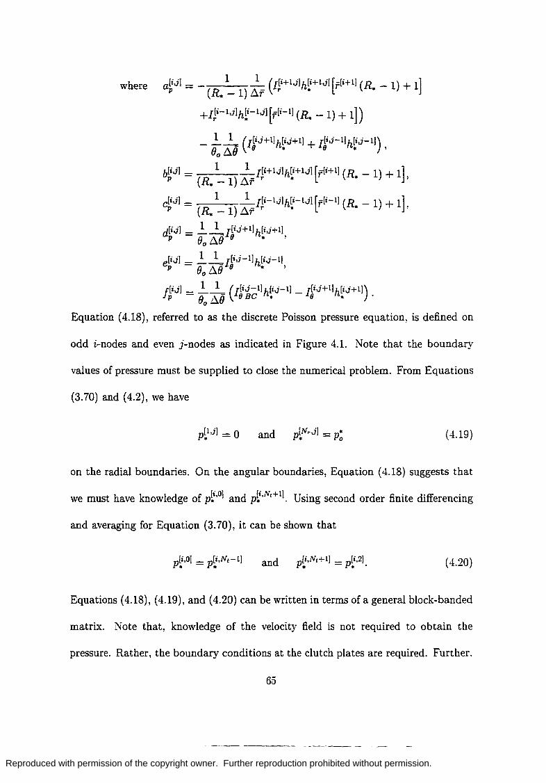
Reproduced with permission of the copyright owner. Further reproduction prohibited without permission.
where a[i,j] = _ 1 1 (I[i+L,i]h[i+L,j] [f[i+L] (R _ 1) + 1] P (R. - 1) I1f T. •
+I~i-l,j]h~-l,j] [f[i-L] (R. - 1) + 1])
_.!. 1_ (/[i,j+L]h[i,j+L] + I[i,j-L]h[i,j-L]) ()o 11() 8 • 9 • ,
b[i,j] = 1 1 I[i+L,j]h[HL,j] [r[HL] (R - 1) + 1] P (R. - 1) ~r T. • ,
e[i,j] = 1 1 /[i-L,j]h[i-L,j] [r[i-LJ (R - 1) + 1] P (R. - 1) ~r T. • ,
d[i,j] =.!. 1_/[i,j+L]h[i,j+L] P ()o 11() 8 * ,
[i,j] _ .!.~l[i,j-L]h[i,j-L] ep - ()o 118 8 • ,
j [i,j] =.!. 1_ (I[i,j-l]h[i,j-L] _ I[i,j+L]hli,j+L]) p ()o 11() 8 Be. 8 • .
Equation (4.18), referred to as the discrete Poisson pressure equation, is defined on
odd i-nodes and even j-nodes as indicated in Figure 4.1. Note that the boundary
values of pressure must be supplied to close the numerical problem. From Equations
(3.70) and (4.2), we have
p~L,j] = 0 (4.19)
on the radial boundaries. On the angular boundaries, Equation (4.18) suggests that
we must have knowledge of p~,O] and p~,Nt+L]. Using second order finite differencing
and averaging for Equation (3.70), it can be shown that
and P[i,Nt+L] = p[i,2] . . . (4.20)
Equations (4.18), (4.19), and (4.20) can be written in terms of a general block-banded
matrix. Note that, knowledge of the velocity field is not required to obtain the
pressure. Rather, the boundary conditions at the clutch plates are required. Further.
65
---------

Reproduced with permission of the copyright owner. Further reproduction prohibited without permission.
the viscosity distribution is assumed to be known.
Again, the above method, which outlines a methodology by which a pressure
distribution may be found, parallels classical derivations of the Reynolds equation.
The additional complication of allowing for variable viscosity across the film demands
numerical treatment in all but the simplest of cases. The analogous steps used to
derive a variable viscosity Reynolds equation are given in AppendL'{ B. Terms in this
variable viscosity Reynolds equation are integrals of the form: Jol zdz and Jol dz. These 1'- 1'-
integrals would have to be evaluated numerically. Further, the discretization of such
a Reynolds equation would demand numerical treatment to solve for the pressure.
Thus, the procedure to follow in solving the variable viscosity Reynolds equation
must use the methodology given above. In other words, both accounting for variable
viscosity and solving a Poisson pressure equation would demand numerical treatment
in either case. The methodology outlined in this section is advantageous because
continuity will clearly be satisfied on a discrete level.
4.2.3 Discrete Axial Velocity Equation
This section discusses the discretization of the differential form of Equation (3.64)
which is used to obtain the axial velocity. It is assumed that the radial and angular
components of velocity are known.
66
- ------ ----

Reproduced with permission of the copyright owner. Further reproduction prohibited without permission.
First, Equation (3.64) is differentiated with respect to the variable z:
(4.21)
which can be rearranged as follows:
(4.22)
where
fvz = (14 ~ 1) [h·:r ([r(R. -1) + 11~i) -[r(R. - 1) + 11~~* (;; + z~;;) 1
1 [ 82v; 8h* f 8v; _82VO) 1
+ (}o h* 8z80 - 80 l 8z + z 8z2 .
Second, Equation (4.22) is discretized on odd i-nodes and even j-nodes:
[r[i] (R* - 1) + 1] (V*[i,j,k+l] _ 2V*[i,j,k] + V*[i,j,k-l]) = _ /i,j,k] (4.23) ~z2 z z z Vz ,
where f[i,j,k] =a[i,j,k]v*[i+l,j,k+l] + a[i,j,k]v·[Hl,j,k-l] + a[i,j,k]v·[i-l,j,k-l] Vz lVz r 2Vz r 3Vz r
+ a[i,j,k]v*[i-l.j,k+l] + a[i,j,k] (V*[i+l,j,k] + V·[i-l,j,k]) H'z r 5V~ r r
+ [i,j,k] *[i,j+l,k+l] + [i,j,k] .[i,j+l,k-lj + [i,j,k] *[i,j-l,k-lj a6Vz Vo a7vz Vo asvz Vo
+ [i,j,k] .[i,j-l,k+l] + [i,j,k] ( .[i,j+l,k] + .[id-l,k]) agVz Vo alOvz Vo Vo ,
67
---------

Reproduced with permission of the copyright owner. Further reproduction prohibited without permission.
a [i,j,k] = 1 1 [h[i,J] [r[i+l] (R - 1) + 1] IVz 2~r~z (R. - 1)· •
_[;01'1 (R. -1) + 1] (h~+l,1L h~-lJ1) (1 + ~~) 1 ' a [i,j,k] = 1 1 [_h[i,j] [r[i+l] (R. _ 1) + 1]
2Vz 2~r~z (R. - 1) •
+ [r[i] (R. - 1) + 1] (h~+l,j] - h~-l,j]) ( 1 - ~:) 1 ' a[i,j,k] = 1 1 [h[i,j] [r[i-lJ (R. - 1) + 1]
3Vz 2~r~z (R. - 1) •
+ [r[,1 (R. - 1) + 1] (h~+lJL h~-ljl) ( 1 - ~~) 1 ' a[i,j,k] = 1 1 [_h[i,j] [r:[i-lJ (D _ 1) + 1]
Wz 2~r~z (R. _ 1). LLoo
-[r[;[ (R. - 1) + 1] (h~+lj[ - h~-ljl) ( 1 + ~~) 1 ' [i,j,k] _ z[k] 1
a5Vz - ~T~Z2 (R. - 1)'
a[i,j,k] = 1 1 [Mi,j] _ (h[i,j+l] _ Mi,J-lJ) (1 + z[k]) 1 6Vz 2~(}~z (}o· • • ~z'
a[i..[,k] = 1 1 [_Mi,j] + (h[i,j+l] _ h[i,J-lJ) (1 - z[k]) 1 7Vz 2~(}~z (}o • • • ~z'
a[i,j,k] = 1 1 [h[i,j] + (h[i,j+l] _ h[i,j-lJ) (1 - z[k]) 1 8Vz 2~(}~z (}o· • • ~z'
a[i,j,k] = 1 1 [_h[i,j] _ (h[i,j+l] _ h[i,j-l]) (1 + z[k]) 1 9Vz 2~(}~z (}o • • • ~z'
[i,j,k] _ z[k] 1 alQVz - ~(}~z2 (}o
As can be seen from Equation (4.23) and Figure 4.1, the angular boundaries do
not present a problem. However, at i = 1 and i = Nr information outside the
domain is required. For example, at i = 1, v;[O,j,k+l], v;[O,j,k], and v;[O,j,k-l j need to be
specified. To circumvent this problem, truncated Taylor series expansions are written
to approximate values outside the domain For example V*[O,j,k]::::: 3v*[2,j,kj_3v*[4.j,kl+ . , r r r
V;[6,j,k]. Only second order truncation error is introduced using these expressions. This
68
--------

Reproduced with permission of the copyright owner. Further reproduction prohibited without permission.
analysis differs from the specification of boundary conditions in that ultimately only
values inside the domain are required.
Since Equation (4.22) is a second order differential equation in z, both no-slip
boundary conditions listed in Equation (3.69) for v; are utilized. Here we have
V;[iJ,l] = v;[iJ,N:] = o. ( 4.24)
Equations (4.23) and (4.24) may be written using a tridiagonal matrix in the same
form as Equation (4.7).
It is not hard to show that if the integral and differential forms of continuity are
satisfied, then Equation (3.64) is satisfied. A simplified proof is given here. Here,
IOh 'V . v dz = 0 is considered the integral form of continuity, and :z ('V . v) = 0 is
considered the differential form of continuity. Let"· v = Ie. Given that :z ('V. v) =
~ = 0, it is known that Ie can be a function of rand () at most. Therefore,
IOh Ie dz = Ie I; dz = feh. But since h =1= 0, and it is given that the integral form
of continuity is zero, we must have Ie = O. Therefore continuity is satisfied. This is
particularly relevant because the previous section which derived the Poisson pressure
equation used the integral form of continuity and this section employed the differential
form of continuity.
4.2.4 Discrete Energy Equation
This section discusses the discretization of Equations (3.68), (3.71), and (3.72). It
is assumed that the velocity components and viscosity are known.
69

Reproduced with permission of the copyright owner. Further reproduction prohibited without permission.
First, Equation (3.68) is written in the form
(4.25)
where the coefficients of the energy equation, (4.25), are defined as follows:
Ar- = Grh:v; A _ _ Grh:vo (.R.-l)' o-[f{R.-l)+l]Oo'
[ * 8h. v;z 8h. voz 1
Af = Grh. V z - 8f (14 - 1) - 89 [f (R* - 1) + 1]00
' (4.26)
fVD = ~.Br [(;;)' + (;;) '].
Second, using Equation (4.2) the terms in Equation (4.26) are discretized:
[
0 ° k] Grh[iJ ]2v *[iJ,k] G h[iJ]2 *[iJ,k] A!J, = • r A~J,k] = r. vB
r (14 - 1)' B [f[i] (14 - 1) + 1]00 '
_ [iJ] Z Z T • * [
(v*[i+l,j,k] + V*[i-l,j,k]) V.[iJ,k]z[k] (h[i+lJ ] _ h[i-1J ])
Az - Grh* 2 - !1f (R. - 1)
( *[H1J+1,k] + *[i-1J+l,k] + *[H1J-1,k] + .[i-l,j-l,k]) -[k] (h[iJ+l] h[iJ-lJ)]
vB VB VB VB Z * -.
- 4!10[f[i] (R. - 1) + l]eo '
[i,j,k]B [ 2 iiJ,k] = J1.. r (v.[i,j,k+l] _ v.[i,j,k-l])
VD 4!1i2 r r
+ 1 ( .[Hl,j+l,k+l] +. *[i-1J+l,k+l] + .[H1J-l,k+l] + *[i-1J-1,k+l] 16~ ~ ~ ~
*[i+lJ+l,k-l] *[i-1J+1,k-l] *[i+1J-l,k-1] *[i-l,j-l,k- lJ)2] -vB - VB - V(J - VB .
( 4.27)
Note that Af, Az, and fv·D are defined on even i-nodes and even j-nodes, while Aij is
defined on odd i-nodes and odd j-nodes.
Third, the finite difference equation, which approximates Equation (4.25), was ob-
tained by applying a three-level fully implicit (3LFI) [16] scheme. Here, the equation
was treated as parabolic in f. Diffusive and convective terms in the i-direction were
handled implicitly using second order central differencing, while the convective term
70
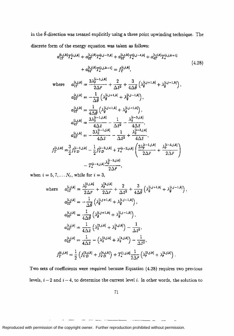
Reproduced with permission of the copyright owner. Further reproduction prohibited without permission.
in the 8-direction was treated explicitly using a three point upwinding technique. The
discrete form of the energy equation was taken as follows:
a[i,j,k]T[i,j,k] + a[i,j,k]T[i,j-2,k] + a[i,j,k]T[i,j-4,k] + a[i,j,k]T[i,j,k+l] IT. 2T. 3T. 4T.
(4.28)
+ a [i,j,k)T[i,j,k-l] _ j.[i,j,k] 5T. - T ,
· . 3A~-I,j,k] 2 3 . . . . [1,J,k] = r + __ + ___ (A~,J+l'k) + A~,J-I,k])
alT 2~f ~z2 4~O S S ' where
[i,j,k] __ ~ (\ ~,j+l,k) + \ ~,j-l,k]) a2T - ~8 AS AS '
[i,j,k] __ 1_ (A~,j+l,k) + A~,j-l,k]) a3T - 4~8 S S '
· . 3A~-1,j,k] 1 A~-3,j,k] [1,J,k] _ z _ __ _ z a4T - 4~z ~z2 -4~-z-'
· . 3A~-I,j,k] 1 A~-3,j,k] [1,J,k):: + --=-.Z __
aST = - 4~z - ~z2 4~z'
j.[i,j,k) =_ j[i-l,j,k) __ ii-3,j,k) + T[i-2,j,k] f + Af 3 1 (3A[i-l,j,k] \ [i-3,j,k))
T 2 VD 2 VD • 2~f -2~-l -f-
A[i-3,j,k) _ T[i-4,j,k]_f __
• 2~f ' when i = 5, 7, ... Nr , while for i = 3,
where . . Al2,j,k] Al4,j,k) ? 3 . . . .
a[I,J,k) = _r __ + _r __ + _-_ + ___ (A~,}+l,k) + A~'}-l,k]) IT 2~f 2~f ~z2 4~O S S '
[i,j,k] __ ~ (\ ~,j+l,k] + \ ~,j-I,k)) a2T - ~8 AS AS '
[i,j,k] = ~ (A~,j+l,k) + A~,j-l,k)) a3T 4~O S S '
a[i,j,k) = _1_ (Al2,j,k) + Al4,j,k]) __ 1_ 4T 4~z z z ~z2 '
~i,j,k] = _1 __ (Al2,j,k) + A(:i,j,k]) __ 1_ aoT 4~z z % ~z2 '
j. [i,j,k] = ~ (f[2,j,k] + f[~,j,k)) + T[I,j,k]_l_ (Al2,j,k] + Al4,j,k]) T 2 v D \I D • 2~f r r .
Two sets of coefficients were required because Equation (4.28) requires two pre\'ious
levels, i - 2 and i - 4, to determine the current level i. In other words, the solution to
71

Reproduced with permission of the copyright owner. Further reproduction prohibited without permission.
the energy equation was obtained by marching forward in radius. This is considered
a three level, fully implicit (3LFI) scheme.
Note that at i = 1, the radial boundary condition in Equation (3.71) may be
written discretely as follows:
T[lj,k) = 1. .. (4.29)
Further, for j = 2 and j = 4, Equation (4.28) suggests we must have knowledge of
the temperature at j = -2 and j = o. However, as periodicity suggests, we have
T[i,-2,k) = T[i,NI-3,k) .. .. , T [i,Q,k) = T[i,NI-l,k) .. .. . (4.30)
In other words, two conditions are given because an upwinding technique is employed
for the angular coordinate. Finally, Equation (3.72) is discretized using spatial second
order differencing:
T [ij,Q) = T[ij,2) * .'
T[ij,N:+l) = T[ij,N:-l) .. ... (4.31)
For each i-level, or discrete radial position, Equations (4.28), (4.29), (4.30), and
(4.31) may be combined and written in terms of a block-banded matrLx. As men-
tioned above, an upwinding technique was used for the term BJoo. This term was
handled implicitly as indicated by the finite difference structure of Equation (4.28).
It was found that this considerably reduced numerical oscillations in the 8-direction
compared with explicit second order central differencing.
4.3 Algorithm Summary
In the previous section, it has been indicated that each numerical problem may
72
-------

Reproduced with permission of the copyright owner. Further reproduction prohibited without permission.
be written in the following general form:
[A]x=y. (4.32)
In general, A is a block-banded matrix, x is an unknown vector corresponding to
one of the unknown dependent variables: v;, v;, v;, p., or T., and y is a known
forcing function corresponding to the right hand sides of Equations (4.7), (4.18),
(4.22)' or (4.28). Further, it has been assumed that the viscosity distribution is
known. However, we require the viscosity-temperature relation (3.53) to be satisfied.
The algorithm used to solve the discrete form of the governing equations which are
coupled by Equation (3.53) is discussed in this section.
It is noted here that several methods exist to solve the system of linear algebraic
equations indicated by Equation (4.32). A numerical scheme which solves a system
of linear algebraic equations having a real banded coefficient matri"{ was chosen. The
scheme computed a lower-upper (LU) factorization [16] of the coefficient matri"{ in
order to check for a singular matrix and to expedite the solution.
The first step in the algorithm was to assume a temperature distribution. The
viscosity may be found on all nodal locations using Equation {3.53} and second order
averaging. For example, to find the viscosity on even i-nodes and even j-nodes, the
viscosity is computed at adjacent radial grid locations using Equation (3.53) and
[" "k] ( ["+1 "kl [" 1 "kl) second order averaging, J1.:J • = ~ J1.: J. + J1.:- .). .
Second, with the estimated viscosity distribution a pressure distribution is ob-
tained by solving the discrete pressure equation, introduced in section 4.3.2, written
in the form of Equation (4.32). Third, the radial and angular components of velocity
73

Reproduced with permission of the copyright owner. Further reproduction prohibited without permission.
are solved using the equations introduced in section 4.3.1. Recall that in this sec-
tion the pressure and viscosity were treated as known quantities. Fourth, the a.xial
velocity is obtained using the equations discussed in section 4.3.3. In this section,
the radial and angular velocity components were treated as known quantities. Fifth,
the temperature is obtained using the equations introduced in section 4.3.4.
A better approximation of the viscosity may be obtained using Equation (3.53).
This iterative procedure is continued until the difference in the temperature fields falls
below a specified error tolerance. In particular, the maximum temperature difference
was required to be less than a specified tolerance.
4.4 Treatment of Clutch Performance Parameters
Upon solving the discretized fluid mechanics problem discussed in the previous
section, the performance parameters are found using numerical integration. N umeri-
cal quadrature is employed.
For example, the application of Simpson's rule on the radial volumetric flow rate
will be discussed here. For convenience, this flow rate is redefined here:
The inner integral can be approximated as follows:
101 . . ~z ( N:-l N:-2)
v* dz ~ I[IJ) = - v*[i,j,l) + v*[i,j,N=) + 4 '" v* [i,j,k) + 2 '" v* [i,j,k) or Q 3 r r ~ r ~ r .
k=2,4,... k=3,<l, ...
After obtaining the approximation for the inner integral, I Q , the flow rate may be
74
---------

Reproduced with permission of the copyright owner. Further reproduction prohibited without permission.
found using a second application of Simpson's rule:
NO [r[i) (R. - 1) + 1]~8 .' . Q........ 9 0 (h["l)I["l) + h[i,Ns)I[I,Ne)
r....... 6 • Q * Q
Ne-1 Ne-2 )
+4 ~ Mi,jj I[i,j) + 2 ~ h[i,j) I[i,j) L....J • Q L....J. Q .
j=2,4,... j=3,5, ...
However, as can be noted from Equation (4.2), v;, and therefore I Q , is defined on even
j-nodes. Using second order averaging for the terms defined in the above equation
on odd j-nodes, the above expression reduces to the following equation:
Ns-l Q; ~ NgOo[r[i) (R. - 1) + 1]~8 2: h~i.i)Ig,j).
j=2,4, ...
Similar expressions were obtained for the normal force, F;, the tangential forces, F;.h'
F;'o, and FO,h' and the frictional moment, l\11'F.
4.5 Numerical Verification
The solutions presented in this section offer specialized check cases for the nu-
merical algorithm. The first section discusses isoviscous axisymmetric solutions and
presents an analytical solution. The second section discusses an isoviscous solution
with radial grooves. In each section, numerical and analytical results are compared.
4.5.1 Isoviscous Axisymmetic Solutions
This section discusses isoviscous axisymmetric solutions of the governing equa-
tions. Since the flow field is incompressible, the assumption of constant viscosity.
fl.. = 1, decouples the energy equation from the momentum equations. We consider
only the hydrodynamic dependent variables: P., v;, vB' and v;. The assumption of
75
-------

Reproduced with permission of the copyright owner. Further reproduction prohibited without permission.
axisymmetry implies all changes in the B.-direction are zero, a~. = O. This is accom-
plished by using a film thickness which is a function of radius only, h. = h. (T.).
Under these conditions, a solution for v; may be obtained using Equations (3.47)
and (3.54):
(4.33)
Equations (3.46) and (3.54) may be used to obtain an expression for v; in terms of
the pressure:
• 1 ap. ( 2 ) vr = --a Z. - z.h. . 2 T.
(4.34)
To obtain a solution for the pressure field, the above equation and (3.45) are integrated
with respect to Z., from Z. = 0 to z. = h •. The following differential equation results
from combining the resulting expressions:
a ( ap.) aT. T.h. aT. = O. (4.35)
The boundary conditions listed in Equation (3.55) may be used with Equation (4.35)
to find the pressure field. Once the pressure is obtained, the radial velocity may
be obtained using Equation (4.34). The axial velocity may be obtained from the
differential form of Equation (3.45) along with Equation (3.54).
An analytical solution was obtained for a radially varying film thickness of the
form h. = 1 + b1 T., where b1 is a constant:
• p~ (2 h ) Vr = 2b h3 Z. - z. * , 2T ••
76

Reproduced with permission of the copyright owner. Further reproduction prohibited without permission.
v" = blP~Z; (Z .. _ 1) ~ 2b2r .. h~ h.. '
= P~ [(2h .. + 1) _ (2hi + 1) In [(h .. - 1) hi]] p.. b 2h2 2h!2 + (h! - 1) h .
2 .. 1 1"
Here, the dimensionless radial inlet and outlet film thicknesses were defined as hi =
1 + b1 and h~ = 1 + b1 R.. The constant b2 is defined as follows:
b = (2h~ + 1) _ (2hi + 1) In [(h~ - 1) hi]. 2 2h .. 2 2M2 (h! - 1) h· o 1 1 0
While the flow is axisymmetric, the film varies linearly with r... In the limit that the
film thickness is constant, b1 = 0, one can show that the axial velocity vanishes using
L'Hopital's rule. Intuition suggests this feature is a necessity from mass continuity
arguments.
Figures 4.2 through 4.5 show a comparison between the analytical and numerical
solutions using R .. = ~, r2. = 1, p .. o = -1.393, and b1 = 1. Using these specified
parameters, the reader can verify that hi = 2, h~ = i, and b2 = 0.043456.
Dimensionless Pressure vs. Qimensionless RaaiL.<s 0.0 I I
-0.5
r i 1
+ NumeriCOI SOlution j - AnOlyticcl Solut;on J
! 1 i
1 i i -1.0~ J
t j
-1.5 '------~ _'--------' 1.0 1.2 1.4 , .6 ~ .8
r.
Figure 4.2: Numerical and Analytical Pressure Profiles
77
-------

Reproduced with permission of the copyright owner. Further reproduction prohibited without permission.
2.0 Redial Velocity
2.0
(a) (b)
Figure 4.3: (a) Numerical and (b) Analytical Radial Velocity Profiles
AnqulC r velocity
2.0 2.0
(a) (b)
Figure 4.4: (a) Numerical and (b) Analytical Angular Velocity Profiles
A convergence study on the velocity components was completed using the following
error equation:
error
Here, VA and VN respectively denote analytically and numerically predicted velocity
components, and N represents the total number of nodes for a particular velocity
component. Summations are taken over the radial, angular, and axial grid locations.
This error was presumed to be a function of grid resolution. The results from this error
78
--------

Reproduced with permission of the copyright owner. Further reproduction prohibited without permission.
<.2
•. 0
(a) (b)
Figure 4.5: (a) Numerical and (b) Analytical Axial Velocity Profiles
analysis are shown in Figure 4.6. In this study, while the computational grid spacings
Error Anal sis of Velocit Components 10-4r-------~------~--~~--~~~-,
2 c Q) 10-6 c 0 ~
E 0 10-8 · u + v, ?:- · " Vs u · .2 10- 10 - Vz Q)
>
10-12~ c '-0 '-'-w
10- 141
0.01 D.: 0 M, 68, 6"2
Figure 4.6: Error Analysis for Isoviscous Axisymmetric Check Case
were varied, the relative size of these grid spacings were held fixed: 6.f = 6.8 = ~Z.
From Figure 4.6, the error in the numerically predicted angular velocity distribution
is round-off error. In other words, there is no truncation error in the prediction of the
angular velocity component. Further, the error in the radial and axial components ap-
pear similar in magnitude over the range of grid spacings examined. The results from
79

Reproduced with permission of the copyright owner. Further reproduction prohibited without permission.
these two components indicate that the measured order of accuracy was 0 (~f3.456)
for v; and 0 (~f3.379) for v;. This is an improvement over the theoretical order of
accuracy, 0 (Af2). While no formal truncation error analysis was completed, it is
believed that this improvement is a result of the symmetry present in the problem.
In addition, the clutch performance parameters, mentioned previously, were ob-
tained for this check case:
F;,h = 0,
where,
b = (h* _ h~) _ ~ I h~ ~ (~ _ ~) _ (2hi + 1) (h~2 - h;2 _ h* h~) 3 0 I 2 n h~ + 2 h* h~ 2h~2 2 0 + I
I 0 I I
+ {h~ ~ 1)2 (2In{h~ -1) -1) _ {hi ~ 1)2 (2In{h; -1) -1)
h*2 h*2 - _0 (2Inh* -1) + _i (2Inh~ -1) + (h*lnh* - h*) - (h~lnh~ - h~) 4 0 4 I 000 I I I
_ I (hi - 1) (h~2 - hi2
_ h* h~) n h~ 2 0 + I ,
I
h*3 h*3 3 h* b4 = 0 - i - - (h*2 - h~2) + 3 (h* - h~) - In .-£. 3 2 0 I 0 I h~ .
I
It should be clear that the analytical expressions are cumbersome for this relatively
simple flow field. Nevertheless, agreement was found between the numerically pre-
dieted performance parameters and the analytical expressions above. For the speci-
fied dimensionless parameters, along with S = 0.598 and € = 8.33 X 10⁻⁴ , the clutch
performance parameters were computed:
Q; = 16.79, F; = 0.456,
80

Reproduced with permission of the copyright owner. Further reproduction prohibited without permission.
F;,Q = -F;,h = -2.843 x 10⁻⁴,
MF = -3.90 x 10⁻⁴, J1.F = 6.23 X 10⁻⁴
•
4.5.2 Isoviscous, Radially Grooved Solution
This solution considers a non-axisymmetric film thickness. The geometry under
consideration is similar to a parallel-step slider bearing, or Rayleigh Step Bearing.
Similar two-dimensional problems are solved by Hamrock [22] in Cartesian coordinates
and Gross [18] in cylindrical coordinates. As in the previous analytical solution,
the lubricant was taken as isoviscous which decoupled the momentum and energy
equations. Results are presented for dimensionless pressure distribution, p ...
The film thickness was defined in parts:
1 O<(J <!lsz. _.. 3
h. = 2 !lsz. < (J < £!lsz. 3 _. 3 (4.36)
1
Unlike the previous section, the film thickness depends on the angular coordinate,
(J., and is not continuous. In Chapter 3, we assumed that there were no severe
gradients in the film thickness. Here, we temporarily relax this assumption and
assume Equations (3.64-3.72) are still valid. We note that this violates the strict
ordering scheme developed earlier so that the solutions obtained are not rational limits
of the Navier Stokes Equations. Nevertheless, such analyses have yielded results which
compare favorably with experiments and are consistent with Hamrock and Gross.
Analytical solutions can be obtained because the pressure adjacent to each parallel
81
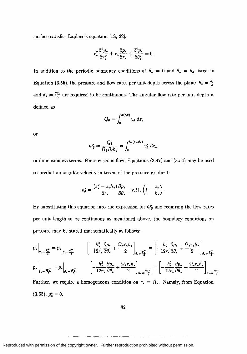
Reproduced with permission of the copyright owner. Further reproduction prohibited without permission.
surface satisfies Laplace's equation [18, 22]:
In addition to the periodic boundary conditions at (). = 0 and (). = (}o listed in
Equation (3.55), the pressure and flow rates per unit depth across the planes 0. = ~
and (). = ~ are required to be continuous. The angular flow rate per unit depth is
defined as
rh(r,O)
Qo = 10 Vo dz,
or
• _ Qo _ rh.(r.,O.) •
Qo - rh~ho - 10 Vo dz.,
in dimensionless terms. For isoviscous flow, Equations (3.47) and (3.54) may be used
to predict an angular velocity in terms of the pressure gradient:
• _ (z; - z.h.) 8p. () (1 _ z.) Vo - 2r* 8(}. + r*H. h*·
By substituting this equation into the expression for Qo and requiring the flow rates
per unit length to be continuous as mentioned above, the boundary conditions on
pressure may be stated mathematically as follows:
p·1 9+ = p·1 9-0.==+ 0.==+ [_ h~ 8p. + n.r.h.] = [_ h~ 8p. + n.r"h*]
12r.8(}. 2 o.=~ 12r" 80. 2 o.=~
[ h~ 8p. n.r.h.] [h; 8p" n.r"h.]
-12r.8(). + 2 o.=¥ = -12r" 8(}. + 2 0.==+ Further, we require a homogeneous condition on r. = R •. Namely, from Equation
(3.55), p~ = o.
82
- ---- ----

Reproduced with permission of the copyright owner. Further reproduction prohibited without permission.
The solution for the pressure distribution, in each region where the film thickness
is continuous, may be stated as follows:
00
p. = L [.an cosh (AnO.) + 'Yn sinh (AnO.) 1 sin (An In T.) (4.37) n=l
The coefficients, .an and 'Yn, are defined for the three separate continuous regions:
Pn =
'Yn =
o
r n (18 sinh A0380 - 22 sinh A0380 - 14 sinh AnOo - 4 sinh 2A380 )
( . 4AnOo . AnOo .
- rn -32smh -3- + 18sinh-3
- + 28smhAnOo
18 . h AnOo 32· h 2AnOo) + sm --- sm--3 3
2r n (18 cosh 2A380 - 32 cosh A~80 + 14)
( 4AnOo AnOo
- r n 18 cosh -3- - 14 + 14 cosh -3- - 14 cosh AnOo
4 h 2AnOo) - cos --3
( 4AnOo AnOo
r n -32 cosh -3- + 18 cosh -3- + 28 cosh AnOo
18 h 5AnOo 32 h 2AnOo) + cos -- - cos--3 3
Here, r n and An are defined as follows:
-12n. [l-R~cosmr] r _ In R. (An)2+4
n - -64 - 98 cosh A"380 + 162 cosh AnOo '
0<0 <&. - * 3
A comparison of the analytical and numerically predicted pressure solutions is
shown in Figure 4.7. The numerical and analytical solutions used the following di-
mensionless parameters: R. = ~, n. = 1, and 00 = 0.3. The infinite series in Equation
(4.37) was truncated after the first one hundred terms.
83

Reproduced with permission of the copyright owner. Further reproduction prohibited without permission.
pre~sure pressure
0..0 0. 10
o.~ o.~
.l 0.00
.l 0.00
_0.05 ..0.05
-o.J.~ -o.J.~
(a) (b)
Figure 4.7: (a) Numerical and (b) Analytical Pressure Profiles using Nr = No = 125
A more detailed comparison was completed by way of a convergence study. The
following equation was used to evaluate the error in the analytical and numerical
solutions:
error
Similar to the previous case, PA and PN respectively denote analytically and numeri-
cally predicted pressure values, and N represents the total number of nodes on which
the solution was evaluated. Since the pressure is independent of z, summations are
taken over the radial and angular indices only. As in the previous case, while the com-
putational grid spacings were varied, the relative size of these grid spacings were held
fixed: I::..f = 1::..0. Figure 4.8 shows the results of this convergence study. Local peaks
in the figure occur when the number of angular nodes, No, equals 37, 61, 85, 109, 133,
and 157. For each of these scenarios, angular grid points lie exactly on the lines 0 = t
and 0 = ~ where the discontinuities in film thickness occur. This can be shown using
Equations (4.1) and (4.3). Considering both cases separately (where angular grid
84
-.---.----

Reproduced with permission of the copyright owner. Further reproduction prohibited without permission.
10-3 E Error Analz::sis of Pressure Distribution
; i
~ c: t a
J1 -::l .D ... - 10-4 (/1
a <Il " ... j ::l (/1 I (/1 :1) " ...
10-5 L ~ Cl..
c: ~
~ :l ... j a ... ...
w
10-61 I
0.001 0.010 0.100 t:J.r. M
Figure 4.8: Error Analysis for Isoviscous Radially Grooved Case
points do and do not lie on the mentioned lines), the error decreases with decreasing
grid spacing. The measured order of accuracy using No = 37,61,85,109,133, and 157
was found to be 0 (~f1.968) and 0 (~f1.950) for the remaining cases.
Once the pressure distribution is known, it is possible to obtain the radial and
angular velocity components via the momentum equations.
• 1 ap. ( 2 ) vr = 2' aT. z. - z.h.
• 1 ap. ( 2 ) (z. ) Vo = 2T. ae. z. - z.h. + n.T. 1 - h.
Note that while the pressure distribution is continuous, ~ is not everywhere con-
tinuous. This is shown in Figure 4.7 for both the exact solution and the numerical
solution. Specifically, at the film thickness discontinuities the pressure gradient is
not continuous. This shortcoming, overlooked throughout hydrodynamic lubrication
theory, renders the angular velocity discontinuous at these planes.
85

Reproduced with permission of the copyright owner. Further reproduction prohibited without permission.
Several statements can be made about this check case. First some general state
ments can be inferred regarding the dependent variables: v;, vo, v;, and p., given an
arbitrary film thickness. If the film thickness is continuous, then v;, vo, p., and 'Vp.
are continuous. If the film thickness, and its derivative are continuous (C1) then v;,
ve, v;, p., and 'Vp. are continuous. However, if the film thickness is discontinuous,
then p. is continuous, but 'Vp. is discontinuous. These comments are justified in Ap
pendix C by considering a simplified two-dimensional lubrication problem. Second,
this geometry could be that of a legitimate clutch problem. Payvar [43, 44] consid
ers this problem with the inclusion of diffusion terms in the angular direction. It
is expected that these terms, and further no slip conditions, are required to smooth
out the discontinuities. Nevertheless, the thin-film limit is an approximation which
attempts to describe the physical problem.
86

Reproduced with permission of the copyright owner. Further reproduction prohibited without permission.
CHAPTER 5
RESULTS
This chapter presents the results obtained for this dissertation. In the first section,
the solution for a sinusoidally varying film is given. Here, the velocity, pressure, and
temperature profiles are presented. In the second section, the effects of variable
viscosity on the constant film case will be examined. Here, the effect on clutch
performance of varying four independent parameters is examined. These results are
compared to the analytical solution of the isoviscous, constant film case. In the third
section, results indicating the effects of grooves are given. This section is divided
into two parts: cavitation results and non-cavitation results. In the cavitation part,
the effects of varying the Sommerfeld number and dimensionless groove depth on the
normal load are given. In the non-cavitation part, the effects of varying groove depth
on several performance parameters are given. In the fourth section, a generalization of
the mathematical model to include heat transfer in the plates is given. The purpose
of this section is to show how the lubrication theory may be coupled to a larger
conjugate problem. Here, results are given for constant film shapes, variable film
shapes, constant viscosity, and variable viscosity.
5.1 Model Solution for a Sinusoidally Varying Film Thickness
In this section, velocity, pressure, and temperature profiles are given for the fol-
87

Reproduced with permission of the copyright owner. Further reproduction prohibited without permission.
lowing film thickness:
h B [ (27r(})] h = ho + ~ 1 - cos 0: . (5.1 )
Note that h is periodic and has the following properties:
where ()' varies between 0 and !l;, and hgB is a constant. In dimensionless terms, the
film thickness is as follows:
h h*B [ (27r(}*)] h* = ho = 1 +; 1 - cos Oa ' (5.2)
where h;B = ~. The dimensionless film thickness is shown in Figure 5.1. Dimen-
0.5
Figure 5.1: Film thickness profile from Equation 5.2, using Nr - 49, NB - 49, R* = 1.3, (}o = 0.1, and h;B = 1.0.
sionless velocity, pressure, and temperature profiles are shown in Figures 5.2 through
5.6. Here, dimensionless parameters which were held fixed for this solution are listed
in Table 5.1.
88

Reproduced with permission of the copyright owner. Further reproduction prohibited without permission.
Figure 5.2: Pressure Profile
€ = 1.0 X 10⁻³ Gr = 4.93 Br = 1.21 x 10⁻³ 0. = -1.0
R. = 1.3 p~ = -4.91 X 10⁻² hgO = 1.0 Bo = 0.1
Ki = 165.83 K2 = 0.663 Kj = 1.5 m = 4.6384
Nr =49 No =49 N z = 25
Table 5.1: CONSTANT PARAMETERS FOR RESULTS PRESENTED IN SECTION 5.1
The pressure distribution, shown in Figure 5.2, satisfies the boundary conditions
given in Equation (3.42). In particular, a radial pressure gradient, evident in the fig-
ure, is partially due to the enforcement of the radial boundary conditions: p. (1, B) = 0
and p. (R., B) = p~. However, the relative angular velocity of the separator plate also
plays a role in determining the pressure distribution. Since the relative angular ve-
locity of the separator plate, r2., is negative, the angular inlet section of the domain
is B. > ~, and the angular outlet section is B. < ~. The dimensionless lubricant
89

Reproduced with permission of the copyright owner. Further reproduction prohibited without permission.
pressure decreases upon entering the inlet section until it reaches a minimum. Beyond
this point, at smaller values of ()., the pressure increases until it reaches a maximum.
The pressure decreases beyond this maximum, and exhibits periodicity as indicated
in Equation (3.42).
o.
0.2
(a) (b)
0·"
0.2 C.2
(c) Cd)
Figure 5.3: Radial Velocity Profiles at (). = (a) 0, (b) 9t, (c) ~, and (d) ~.
The velocity components, shown in Figures 5.3, 5.4, and 5.5, are shown in the
r. - z. plane for four values of () •. All velocity components satisfy the no-slip condi-
90

Reproduced with permission of the copyright owner. Further reproduction prohibited without permission.
tion, indicated by Equation (3.41). Further, a recirculation pattern is evident in the
velocity field.
The temperature distribution, shown in Figure 5.6, satisfies the adiabatic con
ditions, Equation (3.60), at the clutch plates, as well as the periodicty and inlet
temperature conditions given by Equation (3.56). The temperature at the inner ra
dius is equal to the inlet radial temperature, T. = 1. At larger radii, the temperature
of the lubricant increases until it reaches a maximum at the outer radius. In this
scenario, it was found that the maximum temperature occured at (). = ~ and z .. = h.
This may partially be explained by the fact that the pressure gradient is severe at
this location resulting in large viscous dissipation.
5.2 Effects of Variable Viscosity on the Constant Film Thickness Case
In this section, several clutch performance parameters are studied as functions of
four independent parameters: the outer pressure, Po, the inlet temperature, To, the
relative angular velocity, S1d , and the film thickness, ho . The performance parameters
presented are the flow rate, Qr, the normal force, Fz, the tangential force due to vis
cous shearing on the separator plate, F8,Q, the frictional moment, lVIF , the coefficient
of friction, J-LF, and the maximum temperature rise, ~Tma.x. The maximum tempera
ture rise is the largest increase in temperature found in the lubricant domain. In all
cases it was found that the maximum temperature was located at r = Ro, and the
minimum temperature was located at r =~. It is assumed that the film is constant,
h = ho, and the viscosity is given by Equation (3.15) using SAE 10 oil. Constant
91
--------

Reproduced with permission of the copyright owner. Further reproduction prohibited without permission.
parameters which were held fixed are listed in Table 5.2.
Nr =31
~ = 5.0 X 10⁻² m Ro = 6.5 X 10⁻² m (}o = 0.1 rad
Pi = 2.5 Jy[ Pa p=920 ~ c = 2 0 -Y- k = 0.14 mWK • kgK
Table 5.2: CONSTANT PARAMETERS FOR RESULTS PRESENTED IN SECTION 5.2
Assuming that the viscosity is constant, f..L = f..Lo, the solution for the hydrodynamic
variables, Vr , Vo, vz , and p, is as follows:
V z = 0,
(p } ln~i P = Pi + 0 - Pi l&'·
nR.;
In this scenario, the energy equation reduces to the following relation:
fJT a T aVr aVe 2 [() 2 ( ) 2] PCUr ar = k az2 + f..Lo az + GZ '
which may be used with the appropriate boundary conditions,
onr=~
- -- -0 aTl aTl a z z=O - GZ z=ho - ,
{5.3}
{5.-1}
{5.5}
{5.6}
(5.7)
to obtain the temperature. In short, a closed form analytic solution for the tem-
perature field was not obtained for the isoviscous case. Nevertheless, five of the six
92
--"-----

Reproduced with permission of the copyright owner. Further reproduction prohibited without permission.
performance parameters may be stated explicitly:
(5.8)
(5.9)
(5.10)
(5.11)
(5.12)
Equations (5.3-5.12) represent the isoviscous, constant film solution. This solution
is qualitatively compared to numerically predicted, variable viscosity results given in
Figures 5.7 through 5.24.
The effects of varying the outer pressure, Po, are illustrated in Figures 5.7 through
5.12 using To = 300K and nd = -100 r~d. Note that increasing the outer pressure
decreases the pressure difference, Pd = (Pi - Po) It is found that increasing the
pressure difference increases the flow rate, Qr. as shown in Figure 5.7. This trend
is consistent with the isoviscous case given by Equation (5.8). The normal force,
Fz , increases with increasing outer pressure as indicated in Figure 5.8. This trend
is consistent with Equation (5.9) for t = 1.3. Both the tangential force, FO,D, and
the moment }.t[F, decrease with increasing outer pressure as shown in Figures 5.9 and
5.10. This effect is due to the viscosity-temperature relation as it can not be explained
using Equations (5.1O) and (5.11). Both the increasing normal force and decreasing
tangential force with increasing outer pressure lead to a decreasing friction coefficient
93
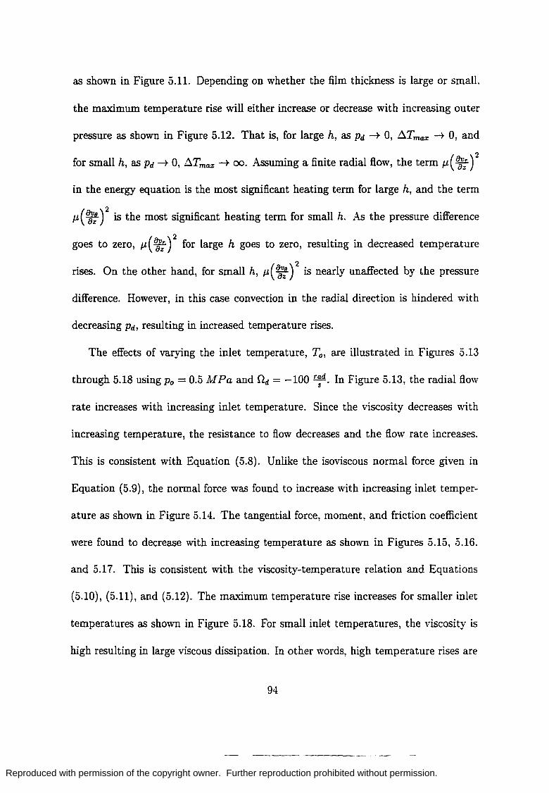
Reproduced with permission of the copyright owner. Further reproduction prohibited without permission.
as shown in Figure 5.11. Depending on whether the film thickness is large or small,
the maximum temperature rise will either increase or decrease with increasing outer
pressure as shown in Figure 5.12. That is, for large h, as Pd ~ 0, ~Tmax ~ 0, and
for small h, as Pd ~ 0, ~Tmax ~ 00. Assuming a finite radial flow, the term Il( ~)2
in the energy equation is the most significant heating term for large h, and the term
Il ( ~ ) 2 is the most significant heating term for small h. As the pressure difference
goes to zero, Il( t:-) 2 for large h goes to zero, resulting in decreased temperature
rises. On the other hand, for small h, Il( ~) 2 is nearly unaffected by the pressure
difference. However, in this case convection in the radial direction is hindered with
decreasing Pd, resulting in increased temperature rises.
The effects of varying the inlet temperature, To, are illustrated in Figures 5.13
through 5.18 using Po = 0.5 NI Pa and nd = -100 r~d. In Figure 5.13, the radial flow
rate increases with increasing inlet temperature. Since the viscosity decreases with
increasing temperature, the resistance to flow decreases and the flow rate increases.
This is consistent with Equation (5.8). Unlike the isoviscous normal force given in
Equation (5.9), the normal force was found to increase with increasing inlet temper-
ature as shown in Figure 5.14. The tangential force, moment, and friction coefficient
were found to decrease with increasing temperature as shown in Figures 5.15, 5.16.
and 5.17. This is consistent with the viscosity-temperature relation and Equations
(5.10), (5.11), and (5.12). The maximum temperature rise increases for smaller inlet
temperatures as shown in Figure 5.18. For small inlet temperatures, the viscosity is
high reSUlting in large viscous dissipation. In other words, high temperature rises are
94

Reproduced with permission of the copyright owner. Further reproduction prohibited without permission.
expected for low inlet temperatures. For the five highest temperature rises shown in
Figure 5.18 the ratio of Brinkman to Graetz numbers varies between 0.042 and O.OB.
Clearly, when this ratio increases (decreasing film thickness) the maximum temper-
ature rise increases. A particular study, involving the relative order of magnitude of
the terms in the energy equation, was performed for this set of operating conditions.
Dimensionless results are reported for the maximum values of convection, conduction,
and viscous dissipation in Table 5.3. The Graetz and Brinkman numbers were varied
Case # 1 2 3 4 5 6
h X 106 (m) 60 8 8 8 8 8
To (K) 400 400 425 450 475 500
Gr x 102 473 8.40 8.40 8.40 8.40 8.40
Br x 104 10 10 7.4 5.4 4.2 3.4
[v*aT.] x 102 r ar. max 9.78 2.37 1.92 1.55 1.30 1.10
[tL(~) 2] YnnT 1.69 1.17 1.41 1.53 1.60 1.63
rtL(~ )2]= 446 0.18 0.31 0.48 0.69 0.92
[Grv* aT. ] X 104 r 8r. max 4620 20.6 16.1 13.0 10.9 9.24
[§.] X 104 az. max
1420 7.00 5.B8 4.96 4.30 3.81
[Brp ((~)2 + (~)2) ] milT X 104 44BO 13.5 12.6 10.8 9.56 8.67
Table 5.3: MAXIMUM VALUES OF TERMS IN DIMENSIONLESS ENERGY EQUATION
by changing the film thickness and inlet temperature respectively. The ma...amum
95
-"._----

Reproduced with permission of the copyright owner. Further reproduction prohibited without permission.
values of the convection, conduction, and viscous dissipation were obtained by exam-
ining the entire domain using finite differencing and determining the maximum. The
results indicate that while a balance between the terms in the energy equation was
achieved, the choice of scaling could be improved. Clearly, the convection, conduc-
tion, and viscous dissipation differ by no more than an order of magnitude for any
individual case. Furthermore, the numbers given in the last three rows indicate that
the contibution of each of these mechanisms is significant. Interestingly, conduction
is consistently the smallest. It is believed that this quantity is the smallest because
of the adiabatic conditions enforced on the clutch plates. However, as indicated,
the dimensionless variables are not 0 (1) for the results examined. This is clearly
illustrated by the terms [v; ~.] and [882').] in Table 5.3.
ur. max z. max
The effects of varying the relative angular velocity, nd, are illustrated in Figures
5.19 through 5.24 using Po = 0.5 NI Pa and To = 300 K. Increasing the magnitude of
the slip speed tends to increase the shear rate leading to high temperatures. Results
regarding the flow rate, normal force, and maximum temperature rise are consistent
with previous discussions. Increasing the slip speed magnitude tends to increase
the tangential force, moment, and friction coefficient. This is consistent with the
isoviscous trends given in Equations (5.10), (5.11), and (5.12).
The effects of varying the film thickness are shown in Figures 5.7 through 5.24.
96
--------

Reproduced with permission of the copyright owner. Further reproduction prohibited without permission.
'. ~
(a) (b)
(c) (d)
Figure 5.4: Angular Velocity Profiles at (J. = (a) 0, (b) ~, (c) ~, and (d) ~.
97
- ----- ------

Reproduced with permission of the copyright owner. Further reproduction prohibited without permission.
15
.. ~
(a) (b)
2
.. ~
(c) (d)
Figure 5.5: Axial Velocity Profiles at (J. = (a) 0, (b) ~, (c) ~, and (d) ~.
98
- ----- -----

Reproduced with permission of the copyright owner. Further reproduction prohibited without permission.
,.0020
(a) (b)
(e) Cd)
Figure 5.6: Temperature Profiles at (). - (a) 0, (b) ~, (e) ~, and (d) ~.
99

Reproduced with permission of the copyright owner. Further reproduction prohibited without permission.
=Iow Rate vs. Film T.,ickness ·0-3~E----~~~~~~~~~~~--~l
~ p. z 0.5 IIPa • • t p.-10I.fPC" 1
! .'~5~ ~ '.' ~'oo ""1 ·0-6~t~ __________ ~r-__________ ~I"
10-5 10~4 10-3
n. Film Thickness. (meters)
Figure 5.7: Variation of Flow Rate with Outlet Pressure
1.30Xl04
Lt ' 1 1.20Xl0
4 ------- P. = 0.5 liP •• j1
Z 4. p. = 1.0 "Po .. - 1 10 10 P •• 1.5 U?a • J 1:00:104f ...---- p. = 2.0 IIPa - J
Normal Force "{So Film Thickress
c f j ~o 9.00 X1 0.3t ~ T. = JOO K j
.,.,,- 0, = -1 00 'Cd/s'~ z .3 • _ 8.00xl0 .. ~ . l ~ i
"- 7.00X1G.3 L /" 1 6.00x 1 0 3 ~g -.;-______ -'=.!,--______ --='.
10-5 10~4 :0-3
n. Film Thickness. (meters)
Figure 5.8: Variation of Normal Force with Outlet Pressure
Tongentici Force vs. Film Thickness
0. s 0.5 uPo x ~
p. ~ 1.0 UPa ..
='. = 1.5 uPo • p. = 2.0 IIPc - -;
1
n, Film ThIckness. (meters)
Figure 5.9: Variation of Tangential Force with Outlet Pressure
100

Reproduced with permission of the copyright owner. Further reproduction prohibited without permission.
To'aue vs. ",1m Thickness
3.0~ 2.5 p •• 0.5 UFo JC ~
p •• '.0 UFo -
~ I p. S 1.5 UPo· 1 ! 2.0 p •• 2.0 UPe - ~
C '~:~':-/l > ::r I
10~-'5-------------10~-~4~-----------1~0-3
", Film Thickness. ~meters)
Figure 5.10: Variation of Friction Torque with Outlet Pressure
Friction ::oefficien! vs. ",1m -hickness 0.008
:l. :: 0.5 UPc'" 1 ••• 1.0 UPo. ,i
C o.=l.SUPo' .~ 0.006 p. = 2.0 liFo - -i
~ f j .. g~ 0.004 ~ ~ ' •• 300 ~ j : 000'[ ~ •. -'00 ."'j
L I 0.000 i"" _________ --=:z-________ ... i.
10-5 10-4 :0-3
1"1, Film ihiCkness. (meters)
Figure 5.11: Variation of Friction Coefficient with Outlet Pressure
~ Maximum TemDera!~re Rise vs. rim Th'ckness ., 100f ;;
:=. oj 80~ p. = 0.5 .... Pe :.: ~
0:
6J p. :: 1.~ \lPo ..
5 p. :: T.5 .... Pe • ;:. = 2.0 .... Po -
"5 ~ r . ::l.
40~ r. = 300 ~ E ! Q" • -100 rOd/sec 1 f §
"f i
E
~ ~ -;;
0 ~
l or :=i 10-5 10-4
10 3
n. Film iniCkness. (meters)
Figure 5.12: Variation of Temperature Rise with Outlet Pressure
101
- ---- ------

Reproduced with permission of the copyright owner. Further reproduction prohibited without permission.
=Iaw Rote 'IS. Film T .,ickness
Figure 5.13: Variation of Flow Rate with Inlet Temperature
Normal Force vs. FOlm Thickress 7800 r[ _---:.;:.;...;,;.;:.;...".:0:..::;;;.-..:= __ .;.;.;..,.-'-".:::..;.;...::.::;"'---,
~ ::t ~ f ~ 7200~ <; f z 7000 r
f 6800
~ J
(: ' J
r, = JCO <. 1
/' i-: ~g ~: j
~:~;5g~o j 1 P, = 0.5 IIPc -i
0 .... -100 rad/sec: i 6600 '=" ___ --,:..-___ ~=-___ -'.
10 10 10 10-3
n, Film ihiclltness. (meters)
Figure 5.14: Variation of Normal Force with Inlet Temperature
Tar.oentici Force vs. FOlm Thickness
n, Film inicl<ness. (meters)
Figure 5.15: Variation of Tangential Force with Inlet Temperature
102
- -'--- ------

Reproduced with permission of the copyright owner. Further reproduction prohibited without permission.
-;"o'oue 'IS. Film Thickness
h, .. 1m Thickness, (meters)
Figure 5.16: Variation of Friction Torque with Inlet Temperature
Friction Coefficient 'IS. Film -hickness 0.008
1
j c: :9 0.006
j
Figure 5.17: Variation of Friction Coefficient with Inlet Temperature
c: Maximum Temperotl.re Rise 'Is. Fi m Th'ckness "i 100l I I I ~ \ } ~ \ ~ ,
ll_' 80l
\ T, • )00 (. J
1'
T. = 350 0(.. l '" f T, = 000 < '
iE~ 64 ~: : ;5g ~ 0 ~ t p. ;E 0.5 uPo
~ 40 ~ 0, $ -100 rOd/sec
j 20~
10 10 h ... 1m Thickness, (meters)
Figure 5.18: Variation of Temperature Rise with Inlet Temperature
103

Reproduced with permission of the copyright owner. Further reproduction prohibited without permission.
=-Iow Rote 'IS. Film T.,ickness '0-3~----~--~~~----~~~--~
.. - -4 E," '0
O. = -SO 'Oc/sec x O. III -100 rOd/Sec .. 0. • -150 rae/sec • O. 2 -200 rae/sec - 1
'.""'" J T •• 300 K 1
·0-6~ __ ----,=-__ ------,1 10- 10 10-3
ci
n, Film Thickness. (meters)
Figure 5.19: Variation of Flow Rate with Relative Angular Velocity
Normal Force vs. Film Thick;-oess 7600 r---~~"--~:":""~";";':';';';"''';'';':';::;';''-=''--...,
1 g 7400 l .; 1 ~ 7200 o. = -50 rae/sec x 1 ... l Q. = -100 rae/sec. J
1. 7000~ i
.... 6800~ ~ 6600 ,=f ..-_____ ---'-_--!::r _______ ... l.
10-5 10~4 10-3
n, Film Thickness, (meters)
Figure 5.20: Variation of Normal Force with Relative Angular Velocity
Tonoenticl Force vs. Film Thickness
Figure 5.21: Variation of Tangential Force with Relative Angular Velocity
104

Reproduced with permission of the copyright owner. Further reproduction prohibited without permission.
To'cue vs. Film Thickness 3.0 r-f ---=-=~"';",";;';":"-=:';':;';';~-----,
f j
2.5
E i 2.0
.; a. 1.5
.§ = 1.0
:i
0.5
o. - -50 ,ed/SJ,. O. ~ -100 'Cd/Se<j ?
0. = -150 'Ca/sea •
1 O.O':=-_____ '::r-____ ---J
10 10 10-3
h, Film inickness, (meters)
Figure 5.22: Variation of Friction Torque with Relative Angular Velocity
Results which are inconsistent with the isoviscous solution can be explained with
the viscosity-temperature relation. For example, the frictional moment shown in
Figure 5.22 reaches a maximum and begins to decrease with decreasing film thickness.
Here, the small film thickness tends to increase the temperature, resulting in reduced
viscosity, which finally leads to a decrease in frictional moment. Another example
is the trend of quantities to approach a limiting curve as the film thickness becomes
large. Note that the tangential force and torque approach a single curve as shown
in Figures 5.9 and 5.10. Again, this can be explained by the fact that at large
film thicknesses, temperature differences in the domain are negligible, resulting in a
fairly constant viscosity. From Equations (5.1O) and (5.11), since lv!F and Fs.o are
independent of Po, a limiting curve is expected for constant viscosity solutions.
A comparison between variable viscosity and constant viscosity predictions is given
in Table 5.4. Constant viscosity clutch performance parameters were based on a nodal
average temperature:
4 "'~r ",ry9 "'~: T[iJ.kj T - L..l=1.3 •... L..J=2.4 ••.• L..l=1.2 •.••
AVG - (Nr + 1) (Ns - 1) Nz
105
---~- ----- ---- --

Reproduced with permission of the copyright owner. Further reproduction prohibited without permission.
F fiction Coefficient vs. Film -hickness 0.008
0, s -50 rca/.ec c: O. - -lCO reals ..
] 0.006
U o u
§ 0.004 ~ .:: : 0.002 :s.
0.0~~~l5'--------10'"'=~""""-----1.-JJ·3 h. Film Thickness. (meters)
Figure 5.23: Variation of Friction Coefficient with Relative Angular Velocity
? Maximum TempefatL.re Rise vs. Fi m Th'ckness ~ 100~ 1 ~ r , g- 80 r" 0, = -50 rca/.ec x .J
j ii 0, = -100 rcd/.ec -0, = -150 rca/.ec ' 5 0, = - 200 rcdlsec -
~ wf 1
f :~ :::~~~ j
J ,~f, \-.,~ ,J, n, Film Thickness. (meters)
Figure 5.24: Variation of Temperature Rise with Relative Angular Velocity
To obtain the average temperature, the existing algorithm was changed merely by
requiring a spatially independent viscosity. In other words, an inital guess for viscos-
ity was made. The pressure, velocity components, and temperature were obtained
as explained in Chapter 4. The average temperature was computed using the above
equation. Finally, an improved guess for the viscosity, based on Equation (3.53), was
made. Again, iteration was required. Thus, the constant viscosity clutch performance
parameters listed in Table 5.4 are based on a reasonable approximation of the bulk
viscosity of the lubricant. Five input states are given in Table 5.3. State 1 is consid-
106
---------- ---- --

Reproduced with permission of the copyright owner. Further reproduction prohibited without permission.
ered Po = 1.5 lv[ Pa, ho = 60 f.1.m, To = 400 K, and nd = -50 r~d. The remaining
four input states show the effects of individually varying the four input parameters
from state 1. Figures 5.25- 5.28 compare velocity, pressure, and temperature profiles
for variable and constant viscosity using the input data for state 1.
Dimensionless Pressure vs. Dimensionless Rcdius 0 j
-2 .. Variaci. Viscosity ~ - Constant Viscosity
~ -4r l i 1
a. r 1 -6r 1
-8~ ~ r l
-10~ ...J
-1) " I ;
1 !
1.0 1.2 1.4 r.
Figure 5.25: Variable and Constant Viscosity Pressure Profiles
(a) (b)
Figure 5.26: (a) Variable and (b) Constant Viscosity Radial Velocity Profiles
While the predicted values of f.1.F, Fz , lV[F, Tmax , and Qr change significantly from
state 1 by individually varying the outer pressure, film thickness, inlet temperature,
and relative slip speed, the variation between the cr.lnstant viscosity model (CY)
107
-_._----

Reproduced with permission of the copyright owner. Further reproduction prohibited without permission.
,A"quIO " veloc·ty ... "'qula,. veloCIty
o'Or
~ _0.5 _o_~~
·0 ·0
_1.1' _t.O
-,~ -,'l
,. . - , . .-(a) (b)
Figure 5.27: (a) Variable and (b) Constant Viscosity Angular Velocity Profiles
._00'
(a) (b)
Figure 5.28: (a) Variable and (b) Constant Temperature Profiles
and the working variable viscosity model (VV) was found to be negligible. Clutch
performance parameters predicted with the constant viscosity model were found to be
within 1.5% of performance parameters predicted with the variable viscosity model.
While only four parameters were examined, it can be concluded from the constant film
case that if a rational method to choose the bulk viscosity is taken, spatial viscosity
variations may be neglected. In practice, this may be difficult as one does not know
a priori which temperature to choose.
In summary, significant variations in the clutch performance parameters were
108

Reproduced with permission of the copyright owner. Further reproduction prohibited without permission.
found by varying input parameters such as the film thickness and inlet temperature.
The viscosity-temperature relation was found to show significant variation from the
isoviscous results given by Equations (5.8-5.12). However, when a good estimation is
made for the bulk viscosity of the lubricant, (such as the viscosity evaluated at the
average temperature) the constant viscosity model produces similar results.
5.3 Groove Studies
In this section, several studies involving grooves in friction plates are presented.
As mentioned previously, grooves are present in friction plates to enhance lubricant
cooling. In the absence of grooves, the model reduces to a parallel plate hydrody-
namic thrust bearing. As a consequence, no load carrying capacity may be generated
except by hydrostatic means. When grooves are present, the model may predict a
hydrodynamic load carrying capacity. Again, our purpose for allowing for arbitrary
geometry is to allow for any groove pattern. However, the results presented in this
section use the following dimensionless groove shape:
1 o ~ (J .. < ~ (1 - xd
h" [8 ] 1 + --::.i.- 2....:. - 1 + Xl Xl-X2 80 ~ (1 - xd ~ (J. < ~ (1 - X2)
h. = 1 +h* ~ (1 - X2) ~ (J * < ~ (1 + X2) (5.13) 9
h" [8 ] 1 - --::.i.- 2....:. - 1 - Xl Xl-X2 80
~ (1 + X2) ~ O. < ~ (1 + xd
1 ~ (1 + xd ~ O. < 00
which is illustrated in Figure 5.29. In Equation (5.13), h; = ~ is the ratio of groove
depth to minimum film thickness, and Xl and X2 are referred to as the major and
109
- --.----- ----

Reproduced with permission of the copyright owner. Further reproduction prohibited without permission.
- X190-
- ~90-
z.
e. 90 (a) (b)
Figure 5.29: (a) Film Thickness Schematic in (). - z. plane and (b) Film Thickness with Xl = 0.4, X2 = 0.2, R. = 1.3, ()o = 0.1 rad, h; = 3.5.
minor groove fractions, respectively. Finally, results presented in this section are
divided into two parts: cavitation and non-cavitation studies. The results presented
in the cavitation part are an isolated set in that negative pressures are predicted using
the existing governing equations. Giimbel's [7, 18, 19, 22] approximation is employed
to predict a load carrying capacity for this section. In the non-cavitation part, and
throughout the remainder of this dissertation, negative pressures are not predicted.
5.3.1 Cavitation Studies
Cavitation refers to the formation of partial gas pockets in a liquid. This phe-
nomenon occurs when the liquid pressure falls below the vapor pressure. In an ideal
incompressible fluid, Batchelor [4] notes that it is possible to predict thermodynami-
cally inadmissible negative pressures. In reality, the assumption of incompressibility
is certainly questionable at these low pressures.
This topic is relevant under groove studies. Birkhoff and Hays [7] cite specific
lemmas regarding increasing and decreasing pressures in converging and diverging
110
---~-----

Reproduced with permission of the copyright owner. Further reproduction prohibited without permission.
domains. In particular, when the local film thickness is less than a specific value.
the pressure will necessarily increase with further reduction in film size. Above this
specific height, which is defined by the geometry and operating conditions of the
lubrication problem of interest, the pressure will decrease. For the domain defined by
Equation (5.13), the pressure will necessarily decrease in the diverging section and
increase in the converging section.
We adopt Giimbel's assumption which states that the vapor pressure is zero and
negative pressures are neglected. Here, the difference between the vapor pressure and
zero is small compared to positive pressures predicted in the lubricant. Physically,
predicting negative pressures infers that a cavity is formed, the no-slip conditions and
the incompressible continuity equation are inappropriate next to the cavity, and the
posed model breaks down. Using the posed model with the assumption of neglecting
negative pressures is a first approximation. Mathematically, Giimbel's assumption is
to ignore negative pressures if the following inequality holds:
(5.14)
which may be shown using Equations (3.25) and (3.73).
For this isolated set of results, we are only concerned with the lubricant load carry-
ing capacity, F;. The numerical analysis is performed exactly as before. However, in
computing the performance parameters, negative pressures are simply ignored. ~ u-
merical results are presented for variable groove depth, h;, and Sommerfeld number,
S. Unless otherwise stated, relevant dimensionless parameters which were held fi.xed
are listed in Table 5.5. Isoviscous results, fl" = 1, are presented in Figures 5.30-5.33.
111

Reproduced with permission of the copyright owner. Further reproduction prohibited without permission.
while variable viscosity results using the viscosity-temperature relation with SAE 10
oil are shown in Figure 5.34.
::~:I Q. 0.000
_0.005
_0.0 10
-O.O~ :i
..:: '."1
Dimensionless FlresSur"e
(a)
1.25
:.20
.' 1.15
1.10
1.05
1.00 L::-:~~~ 0.00 0.02 0.04 0.06 0.08 o. '0
8.
(b)
Figure 5.30: (a) Typical Pressure Distribution and (b) Pressure Contours. (Using S = 968.72 and h; = 3.5.)
Figure 5.30(a) shows a typical pressure distribution predicted by the numerical
model using S = 968.72 and h; = 3.5. Figure 5.30(b) shows the same set of data
displayed as a contour plot. Figure 5.31 shows the zones where cavitation will and
will not occur. Note in Figure 5.31(a), for h; ~ 0 cavitation will not occur. In other
words, without grooves cavitation will not occur. In Figure 5.31(b) the boundary
between regimes reaches a maximum and then tends toward zero as hg ~ 00 • For
large Sommerfeld number, cavitation occurs. These results are consistent with the
two-dimensional Rayleigh thrust bearing theory [18, 22]. Figure 5.32 may be used to
explain Figure 5.31. In this figure, S = 200. Assuming symmetry as shown in Figure
5.30, the maximum and minimum dimensionless pressures have the same magnitude.
Therefore, the groove depth which predicts the largest ma.ximum pressure should
correspond to the position where cavitation is likeliest to occur in Figure 5.31. Further
112
- _. - ---- ----

Reproduced with permission of the copyright owner. Further reproduction prohibited without permission.
in Figure 5.32, as the groove depth goes to zero, the ma..amum dimensional pressure
approaches the inlet radial pressure. This corresponds to P* = 0 in dimensionless
terms. The minimum pressure is found at the radial outlet, P* = p~. On the other
hand, as the groove depth increases, cavitation occurs when the maximum pressure
is larger than p* = ~ = 0.005. The minimum value for maximum pressure occurs
in the zone where cavitation does not occur. As the groove depth gets large, the
maximum pressure value remains finite resulting in an expanded zone of cavitation
to include S = 200 as h; -+ 00. Figure 5.33 shows the normal load as a function of
Sommerfeld number and groove depth. The trends indicate that using an ideal groove
depth with a large Sommerfeld number will increase the load carrying capacity. The
effect of the viscosity-temperature relation is shown in Figure 5.34. Here, S = 33.9
and p~ = -0.02949. The constant viscosity case uses the dimensionless viscosity
based on the inlet temperature throughout the domain. In other words, J.L* = 1 for
the constant viscosity case. Note that the employment of the viscosity-temperature
relation tends to decrease the load carrying capacity. This is consistent with previous
results. That is, while no physical wedge was present for the constant film case.
normal forces computed for variable viscosity were found to be less than constant
viscosity predictions. This can be verified using Equation (5.9), Figure 5.14, and
Table 5.2.
5.3.2 Non-Cavitation Studies
In this section, dimensionless results using variable and constant viscosity, groov
ing and no grooving are presented. Here the effect of varying the groove depth, h;, on
113
~ -------

Reproduced with permission of the copyright owner. Further reproduction prohibited without permission.
Zone of Cavitotion 400 r---~--=;~-=-'='="':'='-=-'--..------,
Zone of Cc,,,itctio,,
1i E ~ l2 ~ 200 u E E rll 111
o 2 4 6 6 200 400 600 !'I; . Dimensionless Groove Depth n; . Dimensionless G,.oove Dept"
(a) (b)
Figure 5.31: Zones of Cavitation and No Cavitation
Maximum Pressure vs. Groove De t"
" ~ 10-2
" c: r
5 = 200.0" j :
E r E 10-3~
~ ,,-,l ~ 10-5f~ ____ ~, ______ ~, _____ ~, ____ ~
0.1 1.0 10.0 100.0 1000.0 n;. Groove Oepth
Figure 5.32: Maximum Pressure vs. Groove Depth
800 'ece
eight dimensionless clutch performance parameters is examined. These parameters
are (1) the flow rate, Q;, (2) the normal load, F;, (3) the tangential force on the
separator plate due to viscous shearing, Fo,o, (4) the tangential force on the friction
plate due to viscous shearing, F;,h' (5) the tangential force on the friction plate due
to pressure, F;,h' (6) the moment, !vIF, (7) the friction coefficient, iJF, and (8) the
maximum temperature T~ax' All results predict positive pressures throughout the
domain, P* > -~. Relevant dimensionless parameters which were held fixed are
listed in Table 5.6.
Results for this section are shown in Table 5.7. Here, the results for no grooves,
114
- ---~- -----

Reproduced with permission of the copyright owner. Further reproduction prohibited without permission.
Dimensionless loco vs. Dimensionless Groove Death
" o
2.0~ , " 1 ,
.3 1.5 ~ " .. " c o
i 1
'in 1.0
~;o,~ E~: 1 0.0 f'--_--'-, __ "'--_--'-, __ -'--_--'1
o 2 4 6 8 10 n;, Dimensionless Groove Depth
Figure 5.33: Normal Load vs. Groove Depth and Sommerfeld Number
Dimensionless load vs. Dimensionless Groove Depth
1020 f ~
~ 1.015t 1 Il ~ Varia ole Viscosity l( 1 C Constant ViSCOSity ~
.~ 1.010 1 ~ ,ooJ , _ ~" j
p; = -0.02949 1 1 1.000 ______ -'-______ -'
o 2 4
"9', Dimensionless Groove Depth
Figure 5.34: Normal Load vs. Groove Depth using Variable and Constant Viscosity
h; = 0, are compared to varying groove depth, h; = 0.5, h; = 1.0, and h; = 2.0.
Further, the variable viscosity model is compared to the constant viscosity model.
The acronyms, VV and CV, used in Table 5.7 denote variable and constant viscosity,
respectively. Note that the flow rate increases as the groove depth increases. This is
expected because a constant pressure difference, p~, is maintained. The normal force
is constant for the CV case and increases for the VV case for increasing h;. This
latter trend was observed for small film thicknesses as shown in Figures 5.8, 5.14,
and 5.20. It is expected that the normal force will remain constant for the CV case
because of the symmetry in pressure shown in the previous section. The tangential
115
----- ----- - --

Reproduced with permission of the copyright owner. Further reproduction prohibited without permission.
forces due to viscous shearing decrease in magnitude as the groove depth increases.
However, the tangential force due to pressure is zero for constant groove depth and
increases as the groove depth increases. This is consistent with Equation (3.79). Note
that in all cases, F;'o + F;,h + F;,h = a as mentioned in Chapter 3. This relation,
which states that the sum of the tangential forces is zero, is in keeping with Newton's
laws since acceleration terms in the momentum equations have been neglected. The
maximum temperature decreases for increasing groove depth because the dominant
heating term in the energy equation is J.L~, and this term decreases for increasing
film thickness.
Figure 5.35 shows velocity vectors at the average radius, T. = l+2R., for the case
where h; = 0.5. Here, the velocity field is essentially a Couette flow in the O-direction.
Velocit reave 1.5
1.01---------' ~ '-------I
- - - - "'" -
," 0 srJ ~ ~ l J ~ ~ ~ ~ j ~ ~ ~ ~ . E :::=; -
F===~====~~== 0.0 -
0.00 0.02 0.04 0.06 0.08 0.10 B.
Figure 5.35: Velocity Vectors at Average Clutch Radius
Note that the axial velocity is significant on the physical wedges.
5.4 Multiple Disk Solutions
In this section, dimensional results for a conjugate lubrication, heat-transfer prob-
116
-------

Reproduced with permission of the copyright owner. Further reproduction prohibited without permission.
lem are given. Here, an assembly of five clutch plates is examined as shown in Figure
5.36(a). Temperature profiles throughout the assembly are predicted.
1\,.,( T • Too) hoo( T - Too)
~ •• t.. ____ 2Lb ~ t.. ____
2Lb z,l 2Ls 2L -r---- --'- -A-S--__________ 1 __
-~-
----------'--Lubricant Film .L
-----'-----.-- h ---'------.---r -----r--- ____ t.. __ ----A---Thickness, h
Lf ---&-- L f Separator plate
LS Adiabatic Backing material •
Friction material Separator plate
5 Backing material • Friction material
1\,.,( T • Toa) (a) (b)
Figure 5.36: Multiple Disk Clutch Conjugate Model Schematic
It is assumed that the ambient conditions, namely the convection coefficient, hoo,
and ambient temperature, Too, are constant. Further, the film thickness between each
plate is identical. These assumptions imply that axial symmetry may be taken about
Zl = 3Ls + 2Lf + 2ho + 2Lb, as indicated in Figure 5.36(b). The thermal energy
equation for each material region is ~~~ = 0, as indicated by Equations (3.50-3.52)
and Figure 5.36(b). The boundary conditions on the temperature field are as follows:
117
---- ------ --

Reproduced with permission of the copyright owner. Further reproduction prohibited without permission.
on z' = 0 :
on z' = Ll :
on z' = Ll + h:
on z' = L2 :
on z' = L3 :
on z' = L4 - h:
on z' = L4 :
on z' = L5 : (5.15)
where,
Ll = 2Ls ,
In the above equation, it has been assumed that L f is the maximum a.'Cial length of
the friction material as shown in Figure 3.2.
Using the fact that the temperature distributions are linear in the a.'Cial direction.
the temperature distributions in the solid material regions may be determined in terms
of the lubricant temperature and its derivative on z' = L 1 , Z' = Ll + h, z' = L4 - h.
and z' = L4 • In other words, we have,
(5.16)
ll8
--------

Reproduced with permission of the copyright owner. Further reproduction prohibited without permission.
where,
k uri k. az' Z':L1
·O<z'<L ' _ _ 1
k uri kaz' / Z':L1+h
; L1 + h :::; z' :::; L2
G1= k uri ko az' Z':L1 +h
; L2 :::; Z' :::; L3
k uri ; L3 :::; z' :::; L4 - h k/ az' , L h z: 4-
0 ; L4 :::; z' :::; L5
TI - .!.. ur I L1 k az' Z'=L1 • Z'=L1
·O<z'<L , _ _ 1
TI - .!..url (L 1 + h) k az' Z'=L1 +h / Z'=L1 +h
t (L2 - L1 - h)]
TI - .!.. ur I [L4 - h] ; L3 :::; Zl :::; L4 - h Z'=L4-h k/ az' Z'=L4-h
TI ; L4 :::; Zl :::; L5 Z'=L4
These ten expressions for C1 and C2 were found from the fourteen conditions in
Equation (5.15). In addition, it may be shown that
(5.17)
Equation (5.17) is used to solve two coupled lubrication problems. The boundary con-
ditions which replace the adiabatic conditions given in dimensionless form in Equation
119

Reproduced with permission of the copyright owner. Further reproduction prohibited without permission.
In=2 In=1
In - 1 T - T
kaT - _ z-h z-h 8z z=h - 2Lt+:;o-2h + ¥:-' (5.18)
and for the second lubricant film are
aTln=2 aTln=1 8z z=h = - 8z z=h'
aTln=2 - =0. 8z z=o
(5.19)
Here, n = 1 denotes the lubrication problem with axial domain L1 :s; z' :s; L1 + h,
and n = 2 denotes the lubrication problem with axial domain L4 - h :s; z' :s; L4. For
n = 1, z = z' - L1, and for n = 2, z = L4 - z'. Note that Equations (5.18) and
(5.19) use a consistent notation convention with the axial coordinate, z, described in
chapter 3. That is, in both lubrication problems we have z = 0 on the separator plate
surface, and z = h on the friction plate surface.
In order to solve this problem, iteration was employed. An initial guess was made
for the second, n = 2, lubricant temperature field. Using this guess, the first, n = 1,
lubrication problem was solved as usual substituting Equation (5.18) for Equation
(3.60). Then, the second lubrication problem was solved by substituting Equation
(5.19) for Equation (3.60). This procedure was continued until the difference between
temperature fields between iteration cycles was negligible.
Upon solving the coupled lubrication problems, the moment delivered to the clutch
may be found. Referring to Figure 5.36(a) and observing symmetry, the net moment.
MF, delivered to the output side of the clutch is the sum of the moments at each
interface:
(5.20)
120
. __ ._----

Reproduced with permission of the copyright owner. Further reproduction prohibited without permission.
The individual moments, AlF=l and AI'F=2, are calculated using Equation (3.84).
An analytical solution was obtained using a zero radial pressure difference, Po = Pi,
a constant viscosity, f.L = f.Lo, and a constant film thickness, h = ho• Under such
conditions, the hydrodynamic variables for the lubricant are
Vr = V z = 0, P=Pi· (5.21)
Equation (5.21) applies to both lubricant films. The temperature field for the assem-
bly shown in Figure 5.36{b) is as follows:
llonar2 [L + ~ + ~ + ...1... _ h _ ~] ho kl 2k k. hoc kl kl
T-Too = llon~r2 [L + ~ + lli + ...1... + 0. _ h] ho kb 2k k. hoc kl kb
llonar2 [L + ~ + ~ + ...1... _ f.a. + 0. + lli] ; L3 :::; Z' :::; L4 - ho
ho kl 2k k. hoc kl kl kb
llonar2 [_(L4- ZI)2 + ~ + lli + lli + ...1... + 2LI] ; L4 - ho :::; z' :::; L4
ho 2kho k kb k. hoc kl
llo~~r2 [¥: + ~ + h: + ¥;- + ~ I] ; L4 :::; Z' :::; L5
(5.22)
For this solution, the temperature condition at r = ~, Equation (3.20), is relaxed.
This condition does not effect the temperature field because the energy equation for
this case reduces to the following expression:
In other words, since the convection terms vanish identically, information at the inner
radius is not convected to the rest of the domain.
121
----- -----

Reproduced with permission of the copyright owner. Further reproduction prohibited without permission.
Relevant dimensional parameters which were held constant for the following results
are listed in Table 5.8. Variable viscosity results are presented using the parameters
associated with SAE 10 oil. The inlet pressure and groove depth were also varied in
this study. The film shape was given by Equation (5.13). In dimensional form, this
equation is as follows:
h + ~ [2.!. - 1 + Xl] o XI-X2 80
h=
h - ~ [28. - 1 - Xl] o XI-X2 80
o :5 () < ~ (1 - xd
~ (1 - xd :5 () < ~ (1 - X2)
~ (1 - X2) :5 () < ~ (1 + X2)
~ (1 + X2) :5 () < ~ (1 + xd
~ (1 + xd :5 () < ()o
(5.23)
Dimensional temperature profiles at the outer radius, r = Ro, are shown in Figures
5.37-5.41. Figure 5.37 shows a comparison between the analytical and numerical
solutions. Here, the viscosity is constant, the pressure difference is zero, ;; = 1. and
the film thickness is constant, ~ = o. Figure 5.38 shows the effect of increasing
the inlet lubricant pressure, Ei. = 2, while holding all other parameters fixed as in po
Figure 5.37. Note that increasing the radial inlet pressure increases the flow rate
resulting in significant convection to cool the clutch. Figure 5.39 illustrates the effect
of using grooves, ~ = 0.5. Compared to Figure 5.38, the temperature distribution
is lower. The temperature distribution resulting from the assumptions of constant
film thickness and variable viscosity is shown in in Figure 5.40. Compared with
Figure 5.38, the temperature distribution is slightly less with variable viscosity. The
temperature distribution resulting from the assumptions of variable viscosity with
122
---------

Reproduced with permission of the copyright owner. Further reproduction prohibited without permission.
16.5~
16.0~
! 155~ I ~
: 15.0~
Numerical and Analytical Solutions i i j
; , i i
1 i 1
~
~ ~ I 1
L J 14.0 .... [ ___ --' ___ -'-_________ '
0.000 0.002 0.004 0.006 0.008
15.Bf
15.sf
~ 15.' i ~ 15.2
,115.0
~ 1'.8
lL.6
n= ,
z" (meters)
lL.''---='" ___ -=r ___ .• 2.98xl0 100'·0 :.02xl0 •
I (net~)
n=2
Figure 5.37: Comparison Between Numerical and Analytical Assembly Temperature Distributions at r = Ro using constant viscosity, 2i = 1, and :.!!Lhh = o.
po 0
grooves is shown in Figure 5.41. Here the temperature distribution is the lowest of
the results presented.
A summary of the clutch performance is given in Table 5.9. It is noted that
while grooving serves to cool the clutch, the frictional moment is reduced. The
model assumption of variable viscosity will give more realistic performance predic-
tions. However, at high temperatures, such as in this scenario (Too = To = 450K),
the viscosity-temperature relation is not very sensitive compared to low temperature
123

Reproduced with permission of the copyright owner. Further reproduction prohibited without permission.
7.101
Numerical SOlution 7.4 I
7.2 ~ c 1 '> ~ 7.0
~ I
~ 6.8~ I i ""6.6
fV 1
i 1
6.41L.........~_--L-__ ----' ___ -'-__ .--J] 0.000 0.002 0.004 0.006 0.008
n=
z' (meters)
n=2 7.]J[.----~-=----
f
0::1 n '~I I -
5.701;----......
~ 71St ! I t /
7l0~ / .) ~
'" 7.15f
7.10,-[ -.-___ -.,-__ _ 2.98.10-5 l00~·o-3 102'10-3
r (r'leters) 5.00'10-5 5.Q2,·0-5 5.0«10-3
r (r'leters)
Figure 5.38: Numerical Assembly Temperature Distributions at r = Ro with constant viscosity, 2i. = 2. and ~h = O. Po . 0
scenarios. In other words, ~I < ~I . This results in approximately the same high T lowT
temperature predictions for equal film shapes as shown in Table 5.9.
In summary, temperature distributions were obtained for a symmetric clutch pack
with five disks. It was assumed that the minimum film thickness, ho, was constant
for all interfaces. The extension of this methodology to incorporate more disks, with
or without the assumption of symmetry, is straightforward. One would solve the
lubrication problem, as developed here, for each lubricant interface between clutch
124
----------

Reproduced with permission of the copyright owner. Further reproduction prohibited without permission.
plates. The appropriate heat flux and temperature continuity conditions should be
used to replace the adiabatic conditions given by Equation (3.60).
Numerical Solution I
4.10 "--_____ --' ___ -'-__ -..J
0.000 0.002 0.004 t (meters)
n='
L6f
f r: ~ LLl
~ .... f---~/ . L2L-t ........--_----. __
2.98x10 .j lOOx·O·J 102.10.3
I (Meters)
0.006 0.008
n=2
Figure 5.39: Numerical Assembly Temperature Distributions at T = Ro and () = 0 with constant viscosity, Ei. = 2, and ~h = 0.5.
po 0
- ._-------

Reproduced with permission of the copyright owner. Further reproduction prohibited without permission.
Numerical Solution 7.0 L I ]
L J
u~ 1
! ~6~ 1 ~J 1
[ f
I 1 r 1
~~ 1
t J 6.0~1 ___ ..:..... ___ -'--~ _ __.l. ___ .......J1
0.000 0.002 0.004 0.006 0.OC8 t (meters)
n=· n=2
Figure 5.40: Numerical Assembly Temperature Distributions at r = Ro with variable viscosity, Pi. = 2, and ~h = o.
po 0
126

Reproduced with permission of the copyright owner. Further reproduction prohibited without permission.
Po ho To nd J.LF Fz }.IfF Tmax Qr
X 10-6 X 106 x102 X 105 X 10-4 x102 X 104
(Pa) (m) (K) (r~d) (N) (N-m) (K) (";3 )
1.5 60 400 -50 VV 6.028 1.059 3.713 401.3 1.768
CV 6.025 1.060 3.715 401.3 1.762
0.15 60 400 -50 VV 9.601 0.6576 3.670 405.5 4.243
CV 9.529 0.6625 3.671 404.5 4.191
1.5 6 400 -50 VV 48.22 1.039 28.85 436.6 0.002179
CV 48.05 1.060 29.63 437.1 0.002210
1.5 60 300 -50 VV 153.2 1.048 92.83 304.3 0.06909
CV 153.2 1.060 94.44 304.4 0.06932
1.5 60 400 -150 VV 18.08 1.060 11.14 401.3 1.769
CV 18.07 1.060 11.14 401.3 1.763
Table 5.4: COMPARISON BETWEEN CONSTANT AND VARLI\BLE VISCOSITY PREDICTIONS FOR THE CONSTANT FILM CASE (CV: CONSTANT VISCOSITY BASED ON AVERAGE TEMPERATURE PREDICTED THROUGHOCT DOMAIN, VV: WORKING VARIABLE VISCOSITY MODEL)
127
--------

Reproduced with permission of the copyright owner. Further reproduction prohibited without permission.
€ = 2.0 X 10⁻⁴ Gr = 0.2628 Br = 2.1527 x 10⁻³ n. =-1
R. = 1.3 p~ = -1.4747 X 10⁻⁴ Xl = 0.4 X2 = 0.2
(Jo = 0.1 Ki = 165.83 K; = 0.663 Kj = 1.5
NT = 31 No =31 N z =31 m = 4.6384
Table 5.5: CONSTANT PARAMETERS FOR RESULTS PRESENTED IN SECTION 5.3.1
€ = 2.0 X 10⁻⁴ Gr = 0.2628 Br = 2.1527 x 10⁻³ n. =-1
R. = 1.3 p~ = -7.3735 X 10⁻² Xl = 0.4 X2 = 0.2
(Jo = 0.1 Ki = 165.83 Ki = 0.663 Kj = 1.5
NT = 31 No = 31 Nz = 31 m = 4.6384
S = 6.7810
Table 5.6: CONSTANT PARAMETERS FOR RESULTS PRESENTED IN SECTION 5.3.2
128
---------
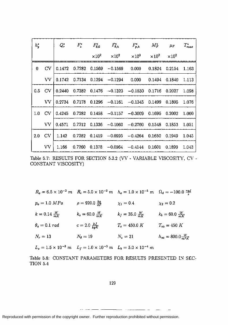
Reproduced with permission of the copyright owner. Further reproduction prohibited without permission.
h* 9 Q; F* z F;'o F;'h F;'h }vI;" J.LF T;ax
x102 X 102 x103 x102 X 102
0 CV 0.1472 0.7282 0.1569 -0.1569 0.000 0.1824 0.2154 1.163
VV 0.1742 0.7134 0.1294 -0.1294 0.000 0.1494 0.1840 1.113
0.5 CV 0.2440 0.7282 0.1476 -0.1323 -0.1530 0.1716 0.2027 1.098
VV 0.2734 0.7178 0.1296 -0.1161 -0.1345 0.1499 0.1805 1.076
1.0 CV 0.4245 0.7282 0.1458 -0.1157 -0.3009 0.1695 0.2002 1.060
VV 0.4571 0.7212 0.1336 -0.1060 -0.2760 0.1548 0.1853 1.051
2.0 CV 1.142 0.7282 0.1419 -0.0993 -0.4264 0.1650 0.1949 1.045
VV 1.166 0.7260 0.1378 -0.0964 -0.4144 0.1601 0.1899 1.043
Table 5.7: RESULTS FOR SECTION 5.3.2 (VV - VARIABLE VISCOSITY, CV -CONSTANT VISCOSITY)
Ro = 6.5 X 10⁻² m ~ = 5.0 X 10⁻² m ho = 1.0 X 10⁻⁵ m Od = -100.0 T~c1
Po = 1.0 }vI Pa p= 920.0 ~ Xl = 0.4 X2 = 0.2
k = 0.14 ~ ks = 60.0 ~i kf = 35 0 ..!!::.. • mK kb = 60.0 ~i
(Jo = 0.1 Tad c = 2.0 k~~ To = 450.0 K Too = 450 K
Nr = 13 No = 19 N z = 21 hoo = 800.0,:rK
Ls = 1.5 X 10⁻³ m Lf = 1.0 X 10⁻³ m Lb = 5.0 X 10⁻⁴ m
Table 5.8: CONSTANT PARAMETERS FOR RESULTS PRESENTED IN SECTION 5.4
129
--------- ---- -

Reproduced with permission of the copyright owner. Further reproduction prohibited without permission.
O.OCC 0.002 0.00' 0.006
n= Ltr-------,.----
'2
/ /
;---.
1: (me,en)
:J~ LQSxtO-3 100x'0-3 J.C2xtC-J
l (Mtt~)
0.008
n=2
Figure 5.41: Numerical Assembly Temperature Distributions at r = Ro and () = 0 . h . bi . . Ei 2 d ~ 0 5 Wit vana e VISCOSlty, =, an h = . . po 0
Input Maximum Temperature Moment
Parameters Tmax , (K) M F , (N - m)
Ei=l ~=O CV po ' ho '
466.14 0.989
Ei = 2 ~ = 0 CV po ' ho '
457.27 0.989
Ei = 2 ~ = 0.5 CV Po ' ho '
454.68 0.923
Ei=2 ~=O VV po ' ho '
456.90 0.957
Ei = 2 ~ = 0.5 VV Po ' ho '
452.74 0.904
Table 5.9: SUMMARY OF CLUTCH PERFORMANCE (VV - VARIABLE VISCOSITY, CV - CONSTANT VISCOSITY)
130
~--.-----

Reproduced with permission of the copyright owner. Further reproduction prohibited without permission.
CHAPTER 6
CONCLUSIONS AND RECOMMENDATIONS
This discussion of the conclusions and recommendations is presented in two sec
tions. In the first section, the results presented in the previous chapter are briefly
discussed and critically reviewed. In the second section, recommendations for future
research are presented in two parts: experimental research and theoretical research. In
the experimental part, benefits and foreseeable difficulties in correlating the hydrody
namic theory are discussed. In the theoretical part, incremental model improvements
as well as boundary and mLxed film lubrication theories are discussed.
6.1 Discussion of Results
In the previous chapter, results were presented for (1) the constant film, variable
viscosity case, (2) groove studies including cavitation and noncavitation, and (3) the
conjugate multiple disk model. These results are discussed and critically reviewed
below.
In the constant film, variable viscosity case an isoviscous analytic solution was
presented for the hydrodynamic variables, Vr , VB, vz , and p, while a simplified form
of the energy equation was given for the temperature, T. This solution was used to
highlight the effects of variable viscosity on six clutch performance parameters (radial
flow rate, normal load, frictional force, frictional torque, friction coefficient, and max
imum temperature rise) while varying four operating conditions (film thickness, inlet
131
----------

Reproduced with permission of the copyright owner. Further reproduction prohibited without permission.
temperature, radial pressure difference, and relative angular velocity). In general,
the results' trends agreed with the expectations of the isoviscous case. Exceptions in
the trends were accounted for using arguments involving the viscosity-temperature
relation. Further, a limited study comparing variable and constant viscosity models
was given for the constant film case. A bulk viscosity, based on the nodal average
lubricant temperature was used for the isoviscous results presented. It was found
that the difference between the variable viscosity results and isoviscous results was
negligible.
In the groove studies, the effects of Gumbel's cavitation assumption on load car
rying capacity were presented as functions of Sommerfeld number and dimensionless
groove depth. In the noncavitation results, eight dimensionless parameters (radial
flow rate, normal load, tangential force due to viscous shearing on the separator
plate, tangential force due to viscous shearing on the friction plate, tangential force
due to pressure, frictional torque, coefficient of friction, and maximum temperature)
were studied as functions of dimensionless groove depth. In both cavitating and
noncavitating parts, results were presented for variable and constant viscosity.
Gumbel's cavitation assumption is based on assuming that the film length de
creases appropriately in the ambient region such that the continuity equation is sat
isfied. In such a scenario, the no-slip boundary conditions are inappropriate in the
ambient region. Such arguments attacking this ad hoc model are noteworthy. Most
importantly, the continuity and momentum equations are elliptic in this formula
tion. Any change in the nature of the solution will influence the solution throughout
132

Reproduced with permission of the copyright owner. Further reproduction prohibited without permission.
the domain. In other words, setting predicted subambient pressures equal to zero
should influence the positive pressures. Giimbel's assumption ignores the nature of
the governing equations.
A more general critique of the groove studies concerns the model's claim to han-
dIe an arbitrary film thickness. Consider the isoviscous Reynolds equation for this
problem:
which may be obtained by integrating the radial and angular momentum equations
with respect to z, enforcing the no-slip boundary conditions on Vr and Vo, integrating
the continuity equation from z = 0 to z = h, integrating the continuity equation
from z = 0 to z = h, enforcing the no-slip boundary conditions on vz , and invoking
Leibnitz's integration rule. For a specified film thickness, h = h (r, (J), the above
equation is a linear partial differential equation in p. To guarantee existence and
uniqueness the coefficients of the pressure derivatives must be continuous within the
domain. This implies that the film thickness must be continuous and differentiable,
Cl, to guarantee a unique solution. Nevertheless, solutions presented in this disser-
tation which violate this criteria predict smoothly varying pressure distributions in
sub domains where h is C1. It is at discontinuities in film thickness where the pressure
gradient is not continuous. In conclusion, we note the following constraint on the film
thickness for lubrication problems: if the pressure gradient in the direction across the
film is taken to be zero, the film shape must be C1 in order to predict a smoothly
varying pressure distribution.
133
---------

Reproduced with permission of the copyright owner. Further reproduction prohibited without permission.
In the multiple disk solutions, two coupled lubrication problems were solved us
ing a straightforward iterative technique. Temperature profiles were presented for
grooves and no grooves, variable and constant viscosity, and finite and zero radial
convection. The results clearly indicate that the clutch temperature can be signifi
cantly reduced with grooves and larger radial pressure gradients. However, the cost
of this temperature reduction is a decreased torque level.
While the model shows how this lubrication theory may be used to model multiple
disk clutch engagement, a critique is that the problem is fairly cumbersome for only
two steady state, scaled lubrication problems. At each iteration level, two lubrication
problems are solved which include solving for the pressure, velocity components,
and temperature iteratively using the viscosity-temperature relation as a constraint
equation. In reality, the physical problem could be significantly more complicated
requiring a more robust model. Some suggestions are recommended in the following
section.
6.2 Recommendations
The following recommendations for future research are presented in two parts: ex
perimental and theoretical. Recommendations in experimental studies are suggested
via stating benefits of correlating theoretical and experimental data. Foreseeable
problems in the experimental method are also mentioned. Theoretical recommen
dations include incremental model improvements as well as mLxed and boundary
lubrication theory models.
134
~------

Reproduced with permission of the copyright owner. Further reproduction prohibited without permission.
6.2.1 Recommendations in Experimental Studies
Before this hydrodynamic theory can be used to model actual clutch engagement,
experimental and theoretical data must be correlated. Benefits of such a correlation
include the establishment of a range of validity of the theory, as well as discovering
new insights concerning the physical problem which may lead to improvements in the
model.
The range of validity of this model is restricted in many ways. If the temperature
is in excess of 600 K, the lubricant will vaporize. As the film thickness gets smaller,
surface roughness and eventually asperity contact become important. On the other
hand, as the film gets larger, different terms, other than those included in this model.
become increasingly important in the governing equations. If the pressure falls below
the ambient pressure, surface tension and compressibility effects become important.
Obviously it would be beneficial to establish a range of validity for this model.
However, a price must be paid to establish such a range. Foreseeable problems in
establishing an experimental to theoretical correlation include fixing the experimental
domain conditions (film thickness, inlet temperature, inner and outer clutch pressures.
slip speed, etc.) to coincide with the input conditions of the theory: as well as installing
the measuring components. Fixing the domain conditions is not simple. Setting the
radial pressure difference, Pd, and the film thickness, h, are two examples. Some
type of measuring device, such as pressure transducer, would need to be installed
at or near the inner and outer clutch radii. Information would likely need to be
acquired remotely for two reasons: (1) the plates move with a relative speed and (2)
135
--------

Reproduced with permission of the copyright owner. Further reproduction prohibited without permission.
splines located at the inner and outer clutch plate radii and connecting hub severely
complicate installation. An alternative to pressure measurement would be flow rate
measurement. This might be easier depending on instrument availability, cost, and
installation. In any case, it should be possible to back out the pressure difference from
the measured flow rate using this theory. Fixing and measuring the film thickness
are also complicated issues. Perhaps fixing the film size could be accomplished by
fabricating separator rings similar to those found in rotating disk couplings [63]. The
use of shims would not be recommended for two reasons: clutch plates have a relative
motion and the shim's presence would disrupt the flow field. The relative motion of
the plates complicates measuring the film size. A distinction between the grooves
and the lands of the friction plates should be recognizable. An alternative to film
thickness measurement would be torque measurement. Here, strain gages could be
installed, the torque could be measured, and the film thickness could be obtained
from the theory.
6.2.2 Recommendations in Theoretical Studies
This discussion of the theoretical recommendations is divided into two parts: in
cremental model improvements as well as mixed and boundary lubrication models.
The incremental model improvements part focuses on previous criticisms, while the
boundary and mixed film part highlights the relevant mechanisms to be included in
future studies and lists pertinent references.
136
--------
Reproduced with permission of the copyright owner. Further reproduction prohibited without permission.
Incremental Model Improvements
Posing the hydrodynamic theory with additional terms in the governing equations,
further boundary and initial conditions, and further constraint conditions would cer
tainly be an improvement from a physical standpoint. Obviously, a greater effort
from a computational perspective as well as a theoretical development perspective
would be required. Perhaps the most critical benefit of such an exercise would be to
show under what conditions the existing theory is valid.
The philosophy used to obtain this dissertation's mathematical model used the
following line of reasoning: (1) state a governing set of equations, (2) nondimen
sionalize the governing equations using the appropriate scales, and (3) transform the
nondimensional equations into a domain of manageable form. Clearly, by comparing
the final conditions in Equations (3.44) and (3.57), information is lost when the film
thickness gradient is infinite. In such a scenario, special treatment should be given
to the nondimensional scales and the geometrical domain transformation.
Some of the shortcomings with the existing cavitation model have been discussed.
Some recommendations are given here. As a first approach it is recommended to allow
for compressibility. This would require an additional equation of state relating the
pressure, temperature, and density. Hamrock [22] cites two such equations relating the
pressure and density for mineral oils. A second approach would be to use a boundary
condition formulation similar to those developed by Swift and Steiber [22, 18], Coyne
and Elrod [11], or Birkhoff and Hays [7] for one dimensional pressure distributions.
In all of these cases, one could argue that this involves the additional specifications
137

Reproduced with permission of the copyright owner. Further reproduction prohibited without permission.
of a surface tension condition, a flow rate condition, and a gas to liquid interface
location condition. It is unknown whether any of the above methods have been
generalized to accommodate two dimensional pressure distributions as assumed in this
model. A third approach would be to examine the entire three dimensional problem.
Here, additional terms in the Navier-Stokes equations and boundary conditions are
appropriate. Ryskin and Leal [51, 52, 53] discuss these types of problems in two
dimensions.
More efficient iterative procedures, such as Newton's method, exist and could
certainly be implemented to satisfy the nonlinearity present due to the viscosity-
temperature relation. Similarly, the coupled lubrication problem's iteration proce-
dure could be solved using a Newton-Raphson method. In general, several iterative
procedures could be incorporated to improve efficiency by accelerating convergence.
6.2.3 Boundary and Mixed Film Lubrication Models
The friction coefficients predicted by this hydrodynamic theory are too low to
adequately describe clutch performance. For the simplest case, the friction coefficient
increases with decreasing film size as indicated by Equation (5.12). To give an idea
of the friction coefficient magnitude predicted by this theory, take f2d = 100 r~d,
/-Lo = 0.104 Ns R m2' 0 = 0.065 m, ~ = 0.05 m, ho = 1.0 X 10⁻⁵ m, and
Pi = Po = 2 X 10⁶ Pa. From Equation (5.12), we have J.tF = 0.03. First it is
noted that this friction coefficient is approximately an order of magnitude larger than
typically predicted using this model. This is because (1) the viscosity is based on a
small temperature, 293 K, for SAE 10, (2) the slip speed is high, and (3) the film
138
- --------

Reproduced with permission of the copyright owner. Further reproduction prohibited without permission.
is small. Notwithstanding, it is noted that the predicted friction coefficient is still
nearly an order of magnitude below typical clutch operating conditions, J..LF ~ 0.1- 0.3
[32]. To remedy this shortcoming, boundary and mixed film lubrication models are
recommended.
As the minimum film size decreases below the clutch plate surface roughness,
ho < a, boundary lubrication is an applicable theory. Only a limited number of the
oretical models have been constructed for this regime of lubrication largely because
the friction is nearly completely dependent on the chemistry of the boundary and the
lubricant. However, according to Bhushan [6], improvements in computer hardware.
increasingly clever algorithms, and recent developments in modeling interatomic in
teractions are having major impacts on the chemical sciences. This is e"idenced by
his discussion on molecular dynamic computer simulations. Nevertheless, usually
one relies on simple models to describe friction in this regime. For example, in the
boundary lubrication regime the normal load is transferred by asperity contact. High
wear rates result from such contacts. Models such as the Archard Wear Law [30] are
used to describe wear. This model is considered ad hoc because the dominant wear
mechanism, such as adhesion, abrasion, or fatigue is rarely discernible [8, 30].
Between the hydrodynamic and boundary lubrication regimes, 1 < t;;z. < 3, lies
the mixed lubrication regime. Here, the normal load between surfaces is transferred
from one surface to another by both asperity contact and the pressurized lubricant.
In general, the friction mechanisms depend on both the chemistry and bulk prop
erties of the lubricant. Unlike the boundary regime, wear is relatively low. Several
139
- ---------

Reproduced with permission of the copyright owner. Further reproduction prohibited without permission.
mixed film lubrication clutch models, which include surface roughness effects and/or
asperity contact, are present in the literature [3, 38, 39, 69]. Models which only in
clude the effect of surface roughness should be incorporated to describe the transition
between contacting and noncontacting regimes. However, to predict realistic friction
coefficients, it is recommended to include both asperity contact and surface roughness
in a mixed lubrication model.
As it stands, the hydrodynamic lubrication theory presented in this dissertation
for disk clutches is an integral part of a broader tribology problem. In order to
incorporate this theory into the larger problem, first one must take the non-trivial
step of modeling asperity contact as indicated above. This will both (1) increase
the clutch temperature given realistic operating conditions and (2) increase the pre
dicted friction coefficient. Towards this end, a serious review of contact mechanics
[33] is recommended. Second, one must determine the limits of each of the theories.
In previous discussions, it was indicated that the film thickness is not known a pri
ori. Rather, the normal load, treated as a derived quantity in this dissertation, is
known. Typically, given a load, the film thickness is obtained iteratively by solving
boundary, mixed, and hydrodynamic lubrication problems. The appropriate regime
is determined by comparing the predicted film thickness to the surface roughness.
1-10
-------

Reproduced with permission of the copyright owner. Further reproduction prohibited without permission.
APPENDIX A
This appendix will give the derivation of Equation (3.60) using Equations (3.57)
and (3.59). For convenience, both equations are restated here:
T.! = T.! ' z;=l zj=O T.! = T.! ' zi=Li+1-h. z.=h.
T. ! = T.!, EiT'. ! = &1'. ! = 0, z;=l z.=O 8z;, z;=o 8z; z;=o
k'bLj &1'.! EiT'.! k; &1'.! EiT'.! kiL'b 8z; z;=l = 8zi Zj=o' L; 8z; z;=l = 8z. z.=o'
(.·1.1)
kj EiT'. ! &1'. ! Lj 8zi zi=Li+1-h. = - 8z. z.=h.'
T. = C{ (r., f).) zj + ct (r., f).) ,
T. = C~ (r., f).) z; + C~ (r., f).) , (..1.2)
T. = Cf (r., f).) z; + c~ (r., 9.).
Substituting the expressions for the temperature fields given in Equation (..1.2) into
the eight expressions given by (A.1), we have
(04.3)
c{ (Lj + 1- h.) +ct = T.lz.=h.' (A...!)
C: +C~ =T.I ' z.=o
(.-L5)
Cb -0 1 - , (04.6)
C: = 0, (..1.7)
(..1.8)
141

Reproduced with permission of the copyright owner. Further reproduction prohibited without permission.
k;cs _ aT. I 1- .
L; 8z. z.=o· (.-l.9 )
k~ c{ = _ aT. I . Lf 8z. ;;.=h.
(.-l.1O )
Here, we have eight linear algebraic equations in the ten unknowns: C~, c~, Ct,
ct, C:, C~, T.lz.=o' T.lz.=h.' fz: Iz.=o' and fz: IZ.=h.' which are in general functions
of r. and (J •• Treating T.lz.=o and T.lz.=h. as known quantities, the solution to the
remaining eight unknowns is as follows:
c~ = Cf = C{ = aT. I = aT. I = 0, 8z. z.=o 8z .. ;;.=h.
(.-1.11)
C~ =ct =T .. I ' z.=h. (.-l.12)
C~=T .. I . z.=O (.-1.13)
From Equation (A.11), the adiabatic conditions listed in Equation (3.60) are evident.
From (A.12) and (.4.13), we see that the temperature distribution in both the backing
and friction materials is T. = T. Iz.=h.' and in the temperature distribution in the
separator plates is T. = T. Iz.=o'
142
----------

Reproduced with permission of the copyright owner. Further reproduction prohibited without permission.
APPENDIX B
This appendix gives the derivation of the variable viscosity Reynolds equation.
This derivation is based on the validity of Equations (3.45)-(3.48) and (3.54). For
convenience, these equations are presented in dimensional form here:
(B.l)
ap _ ~ (J-L avr) ar - az az ' (B.2)
! ap = ~ (f-L ave) r ao az az ' (B.3)
ap =0 az ' (BA)
on z = 0: Vr = Vz = 0, (B.5)
on z = h (r, 0) : Vr = Ve = V;: = o. First, Equation (B.l) is integrated from z = 0 to z = h:
rh [a (rvr ) aVe av;:] d _ 10 ar + ao + r az z - o. (B.6)
Making use of Leibnitz's rule and enforcing the no-slip conditions given in Equation
(B.5), Equation (B.6) may be written as follows:
(B.7)
Second, the velocity components, Vr and Ve, are obtained. From Equation (BA),
the pressure is independent of z. This allows one to integrate Equations (B.2) and
(B.3) with respect to z holding ~ and ~ fixed. Enforcing the no-slip conditions
143

Reproduced with permission of the copyright owner. Further reproduction prohibited without permission.
again, the velocity components may be written as follows:
Vr = - - dz - - dz , ap [Io z z' , foh ~ dz Ioz
1 '1 aT 0 J1. foh ; dz 0 J1.
(B.8)
1 ap [1Z z' foh ~ dz In z 1 1 [foZ 1 dZ'l V8 = - afJ - dz' - h ': - dz' + ndT 1 - h ~ .
T 0 J1. ho - dz 0 J1. fo - dz I/o I/o
(B.9)
Third, the integrals in Equation (B.7) may be found using Equations (B.8) and
(B.9):
Ioh ap [Ioh Ioz
Z' foh ~ dz Ioh Ioz 1 1 Vr dz = -a - dz' dz - h ': - dz' dz ,
o TOO J1. fo ;; dz 0 0 J1.
{h V8 dz =~ aaPfJ [{h r Zl dz' dz _ f~ ~ dz {h (Z ~ dz' dZ] Jo T Jo Jo J1. fo ;; dz Jo Jo f.L
[ II: Ioz !; dz' dZ]
+ ndT h - h 1 . 10 ;; dz
Finally, substituting these expressions into (B.7)' the variable viscosity Reynolds
equation is as follows:
T - T - - dz' dz - p. - dz' dz a ( ap [Io h Ioz z' fl: ~ dz Ioh Io z
1 ] ) aT aT 0 0 J1. fl: ; dz 0 0 f.L
a ([Ioh Io Z
z' II: ~ dz Ioh Io z 1 ] ) + afJ - dz' dz - h ~ - dz' dz
o 0 f.L fo ;; dz 0 0 f.L (B.lO)
_ _ 2 ~ [ _ foh foz ; dz' dzl - ndT
afJ h hl . fo ;; dz
For the isoviscous case, J1. = J1.o, Equation (B.10) simplifies to the following expression:
144
• ~- ------- ---- ~-

Reproduced with permission of the copyright owner. Further reproduction prohibited without permission.
APPENDIX C
This appendix will give the velocity, pressure, and stream function for an arbitrary
film shape. Emphasis is placed on the continuity and differentiability of film shapes.
The simplified lubrication problem studied here is two-dimensional and ismiscous.
The relevant governing equations and boundary conditions are taken as follows:
mass: 8u 8w_
O 8x + 8z - ,
x-momentum: 8p 82u 8x = /-L 8z2 '
z-momentum: 8p =0 8z '
on z = 0: u=U, w=O, no - slip conditions:
on z = h (x) : u =W = O.
on x = 0: pressure conditions:
onx = L: P=Po·
Here the velocity is specified on the surfaces z = 0 and z = h (x), and the pressure
is specified at the inlet, x = 0, and the outlet, x = L. Since the pressure and film
thickness depend on x only, partial derivatives will be replaced by ordinary derivatives
where appropriate.
The x-component of velocity may be stated in terms of the pressure gradient as
follows:
U = -- z - hz + U 1 - - . 1 dp ( 2 ) ( Z) 2/-L dx h
145

Reproduced with permission of the copyright owner. Further reproduction prohibited without permission.
To obtain the pressure, it is convenient to use the following integral form of the
continuity equation:
~ rh u dz = ~ [_l!.... dp + Uh] = 0,
8x 10 dx 12JL dx 2
which may be written as the following Reynolds equation:
~(h3dP) =6JLUdh
. dx dx dx
The z-component of velocity may be obtained from the continuity equation:
w = _~ [rfP (z3 _ hZ2) _ dp dh Z2]_ Uz2
dh. 2J.L dx2 3 2 dx dx 2 2h2 dx
Streamlines may be obtained once a stream function has been defined. A suitable
stream function may satisfy the following conditions:
81jJ 81jJ -=u, 8z
--=W. 8x
The stream function for this generalized lubrication problem is as follows:
Clearly, the velocity components and stream function depend on the film thickness.
pressure, and their derivatives.
In order to justify some of the statements made at the end of Chapter 4, consider
the following continuous, non-differentiable film shape:
a :::; x :::; nL
nL:::; x ~ L
146
---------

Reproduced with permission of the copyright owner. Further reproduction prohibited without permission.
This is shown in Figure C.1. The pressure may be found in each continuous zone using
the Reynolds equation. Since the Reynolds equation is a second order differential
equation, two boundary conditions must be supplied for each zone. This requires a
total of four conditions. The standard assumptions [I8! 22] are to require continuity
of flow rate per unit length and pressure as additional conditions.
plx=nL+ = plx=nL-,
[ h3 dp hUl [ h
3 dp hUl
I2JL dx + 2 x=nL+ = I2JL dx + 2 x=nL-'
Given these conditions, the pressure may be stated in parts as follows:
P(X)=
where,
6n [ 1 x I+H --o n
Ho (1 + Ho) (-1- Ho + n)
(-2 - 4Ho - 2H; + 2n + 3nHo) (1 + Ho _ -;::)2 2 + Ho - 2n 1
+ -2 - 4Ho - 2H; + 2n + 3nHo 6n (X - 1)
Ho (-2 - 4Ho - 2H; + 2n + 3nHo)
x X=-,
L
n:::;X:::;I
vVe find that the pressure and its derivative are continuous at x = nL. Further.
the velocity, u, and stream function, 'I/J, are continuous. However, the z-component
of velocity is not continuous across x = nL. These results are in keeping with the
general remarks at the end of Chapter 4. Streamlines using a dimensionless stream
function, 'I/J* = s:u' with n = 0.7 and Ho = 1.0, are given in Figure C.2. Here,
Z-.L - Sh'
147
--------

Reproduced with permission of the copyright owner. Further reproduction prohibited without permission.
p p
U Figure C.I: Continuous, non-differentiable film shape
Streamlines 2.0
1.5
N 1.0 ~ __ ---~
~ j J J I
1 ~
0.5 r--------------.:J..,
0.0 ~ __ ...L....._ __ _'__~ _ _'_~_~_~__'
0.0 0.2 0.4 0.6 0.8 1.0 x
Figure C.2: Dimensionless streamlines using n = 0.7 and Ho = 1.0
148
---------

Reproduced with permission of the copyright owner. Further reproduction prohibited without permission.
BmLIOGRAPHY [1] Barcilon, V. and Pedlosky, J. (1967) "Linear theory of rotating stratified fluid
motions," Journal of Fluid Mechanics, vol. 29, part 1, pp. 1-16.
[2] Barcilon, V. and Pedlosky, J. (1967) "On the steady motion produced by a stable stratification in a rapidly rotating fluid," Journal of Fluid Mechanics, vol. 29, pp. 673-690.
[3] Bardzimashvili, N. G. and Yashvili, S. G. (1987) "Study of Multi-disk Oil Friction Clutch Engagement," Soviet Journal of Friction and Wear, vol. 8, no. 2, pp. 57-64.
[4] Batchelor, G. K. (1967) An Introduction to Fluid Dynamics, Cambridge University Press, Cambridge.
[5] Batchelor, G. K. (1951) "Note on a Class of Solutions of the Navier-Stokes Equations Representing Steady Rotationally-Symmetric Flow," The Quarterly Journal of Mechanics and Applied Mathematics, vol. 4, pp. 29-41.
[6] Bhushan, Bharat (1995) Handbook of Micro/Nano Tribology, CRC Press, Boca Raton.
[7] Birkhoff, G. and Hays, D. F. (1963) "Free Boundaries in Partial Lubrication." Journal of Mathematical Physics, vol. 42, no. 2, pp. 126-138.
[8] Briscoe, B. J. and Evans, P. D. (1989) "The Infiuece of Asperity Deformation Conditions on the Abrasive Wear of Gamma Irradiated Polytetrafluoroethylenes," Wear, vol. 133, pp. 47-64.
[9] Chew, J. W. (1985) "Computation of convective laminar flow in rotating cavities," Journal of Fluid Mechanics, vol 153, pp. 339-360.
[10] Cole, J. A. (1974) ''Taylor Vortices ,vith Short Rotating Cylinders," Journal of Fluids Engineering, vol. 96, pp. 69-70.
[11] Coyne, J. C. and Elrod, H. G. (1971) "Conditions for the Rupture of a Lubricating Film - Part 2 New Boundary Conditions for Reynolds Equation," Journal of Lubrication Technology, Series F, pp. 156-167.
[12] Di Prima, R. C. and Swinney, H. L. (1985) "Instabilities and Transition in Flow Between Concentric Rotating Cylinders," Hydrodynamic Instabilities and the Transition to Turbulence, H. L. Swinney and J. P. Gollub, eds., pp. 139-180, Springer, Berlin.
[13] Dorinson, A. and Ludema, K. C. (1985) Mechanics and Chemistry in Lubrication Elsevier Science Publishers B. V., Amsterdam.
[14] Eringen, A. C. (1967) Mechanics of Continua, vViley, New York.
[15] Evans, G. and Grief, R. (1987) "A Numerical Model of the Flow of Heat Transfer in a Rotating Disk Chemical Vapor Deposition Reactor," Journal of Heat Transfer, vol. 109, pp. 928-935.
1-19
- ------

Reproduced with permission of the copyright owner. Further reproduction prohibited without permission.
[16] Fletcher, C. A. J. (1991) Computational Techniques for Fluid Dynamics. voL l. Springer-Verlag, Berlin.
[17] Fletcher, C. A. J. (1991) Computational Techniques for Fluid Dynamics, vol. 2, Springer-Verlag, Berlin.
[18] Gross, W. A. and Matsch, 1. A. and Castelli, V. and Eshel, A. and Vohr, J. H. and Wildmann, M. (1994) Fluid Film Lubrication, John Wiley & Sons, New York.
[19] Giimbel, L. and Everling, E. (1925) Reibung und Schmierung im Maschinenbau. M. Drayn, Berlin, 1925.
[20] Guo, Z. Y. and Zhang, C. M. (1992) "Thermal drive in centrifugal fields - mLxed convection in a vertical rotating cylinder," International Journal of Heat and Mass Transfer, vol. 35, no. 7, pp. 1635-1644.
[21] Hadid, A. H. (1993) "Chaotic flow in rotating lid cavities," Physics of Fluids A, vol. 5, no. 8, pp. 1939-1947.
[22] Hamrock, B. J. (1994) Fundamentals of Fluid Film Lubrication, Mc-Graw HilL New York.
[23] Hamrock, B. J. and Jacobson, B. O. (1984) "Elastohydrodynamic Lubrication of Line Contacts," ASLE Transactions, vol. 27, no. 4, pp. 275-287.
[24] Hersey, M. D. (1966) Theory and Research in Lubrication, John vViley and Sons Inc., New York.
[25] Hirsch, C. (1988) Numerical Computation of Internal and External Flows, vol. 1, John Wiley and Sons, Chichester.
[26] Hoglund, E. and Jacobson, B. (1986) "Experimental Investigation of the Shear Strength of Lubricants Subjected to High Pressure and Temperature," Journal of Tribology, vol. 108, pp. 571-578.
[27] Homsy, G. M. and Hudson, J. 1. (1969) "Centrifugally driven thermal convection in a rotating cylinder," Journal of Fluid Mechanics, vol. 35, part 1, pp. 33-52.
[28] Houpert, L. G. and Hamrock, B. J. (1986) "Fast Approach for Calculating Film Thicknesses and Pressures in Elastohydrodynamically Lubricated Contacts at High Loads," Journal of Tribology, vol. 108, no. 3, pp. 411-420.
[29] Hussain, A. and Biswas, S. and Athre, K. (1992) "A new viscosity-temperature relationship for liquid lubricants," Wear, Vol. 156, pp. 1-18.
[30] Hutchings, 1. M. (1992) Tribology: Friction and Wear of Engineering Materials. CRC Press, Boca Raton.
[31] Ichihashi, T. (1994) "Recent Developments in Lubricating Oils for vVet Clutches and Brakes," Japanese Journal of Tribology, vol. 39, no. 12, pp. 1461-1470.
[32] Ito, H. and Fujimoto, K. and Eguchi, M. and Yamamoto, T. (1993) "Friction Characteristics of a Paper-Based Facing for a vVet Clutch under a Variety of Sliding Conditions," STLE Tribology Transactions, vol. 36, no. 1, pp. 134-138.
[33] Johnson, K. 1. (1985) Contact Mechanics, Cambridge University Press, London.
150
---------

Reproduced with permission of the copyright owner. Further reproduction prohibited without permission.
[34] Johnson, K. L. and Tevaarwerk, J. L. (1977) "Shear behavoir of elastohydrodynamic oil films," Proceedings of the Royal Society of London A., vol. 356, pp. 215-236.
[35] Lance, G. N. and Rogers, M. H. (1962) ''The axially symmetric flow of a viscous fluid between two infinite rotating disks," Proceedings of the Royal Society of London A., vol. 266, pp. 109-12l.
[36] Millsaps, K. and Pohlhausen, K. (1952) "Heat Transfer by Laminar Flow From a Rotating Plate," Journal of Aeronautical Sciences, vol. 19, pp. 120-126.
[37] Minkowycz, W. J. and Sparrow, E. M. and Schneider, G. E. and Pletcher, R. H. (1988) Handbook of Numerical Heat Transfer, John Wiley and Sons, New York.
[38] Natsumeda, S. and Miyoshi, T. (1994) "Numerical Simulation of Engagement of Paper Based Wet Clutch Facing," Transactions of the ASME, vol. 116, pp. 232-237.
[39] Osani, H. and Ikeda, K. and Kato, K. (1990) "Relations Between Temperature in Friction Surface and Degradation of Friction Materials During Engaging of \-Vet Friction Paper," SAE Transactions, vol. 99, sect. 6, pp. 724-731.
[40] Panton, R. L. (1984) Incompressible Flow, Wiley, New York.
[41] Patir, N. and Cheng, H. S. (1978) "An Average Flow Model for Determining Effects of Three-Dimensional Roughness on Partial Hydrodynamic Lubrication," ASME Journal of Lubrication Technology, vol. 100, pp. 12-17.
[42] Patir, N. and Cheng, H. S. (1979) "Application of Average Flow Model to Lubrication Between Rough Sliding Surfaces," ASME Journal of Lubrication Technology, vol. 101, pp. 220-230.
[43] Payvar, P. (1991) "Laminar heat transfer in the oil groove of a wet clutch" Int. J. Heat Mass Transfer., vol. 34, no. 7, 1792-1798.
[44] Payvar, P. and Lee, Y. N., and Minkowycz, W. J. (1994) "Simulation of heat transfer to fluid flow in radial grooves of friction pairs," International Journal of Heat and Mass Transfer, vol. 37, pp. 313-319.
[45] Pearson, C. E. (1965) "Numerical solutions for the time-dependent viscous flow between two rotating coaxial disks,:' Journal of Fluid Mechanics, vol. 21, pp. 623-633.
[46] Peyret, R. and Taylor, T. D. (1983) Computational Methods for Fluid Flow, Springer-Verlag, New York.
[47] Quast, P. and Smith, A. (1993) "Experimental Design and Analysis of ClarkHurth Clutch Systems", Technical Report, University of Notre Dame, Notre Dame, Indiana.
[48] Robertson, B. J. (1935) An Investigation of Motor Oils. (Bulletin of the University of Minnesota, Engineering Experimental Station, Bulletin No. 10), :\Hnneapolis.
151
----------

Reproduced with permission of the copyright owner. Further reproduction prohibited without permission.
[49] Robertson, B. J. (1936) Motor Oils for Winter Use. (Bulletin of the University of Minnesota, Engineering Experimental Station, Bulletin No. 11), Minneapolis.
[50] Roelands, C. J. A. (1966) Correlational Aspects of the Viscosity-TemperaturePressure Relationship of Lubricating Oils, Druk, V.R.B., Groingen, Netherlands.
[51] Ryskin, G. and Leal, L. G. (1984) "Numerical solution of free-boundary problems in fluid mechanics. Part 1. The finite-difference technique," Journal of Fluid kfechanics, vol 148, pp. 1-17.
[52] Ryskin, G. and Leal, L. G. (1984) "Numerical solution of free-boundary problems in fluid mechanics. Part 2. Buoyancy-driven motion of a gas bubble through a quiescent liquid," Journal of Fluid Mechanics, vol 148, pp. 19-35.
[53] Ryskin, G. and Leal, L. G. (1984) "Numerical solution of free-boundary problems in fluid mechanics. Part 3. Bubble deformation in an a.xisymmetric straining flow," Journal of Fluid Mechanics, vol 148, pp. 1-17.
[54] Schlichting, H. (1960) Boundary Layer Theory, McGraw Hill, New York.
[55] Schulz, N. (1990) "Physical Relationship Between the Axial Gas-Lubricated Plain Bearings and a Clutch," SAE Transactions, vol. 99, sect. 2, pp. 567-580.
[56] Scott, W. and Suntiwattana, P. (1995) "Effect of Oil Additives on the Performance of a Wet Friction Clutch Material," Wear, vol. 181-183, no. 2, pp. 850-855.
[57] Shigley, J. E. (1977) Mechanical Engineering Design, Third Edition, McGraw Hill, New York.
[58] Singh, H. and Gulati, 1. B. (1986) "Influence of Base Oil Refining on the Performance of Viscosity Index Improvers," Wear, Vol. 118, pp 33-56.
[59] Solt, M. B. (1990) "Optimizing Automatic Transmission Lining Load Distribution Using Finite Element Analysis," SAE Transactions, vol. 99, sect. 6, pp. 777-787.
[60] Stebar, R. F. and Davison, E. D. and Linden, J. L. (1990) "Determining Frictional Performance of Automatic Transmission Fluids in a Band Clutch." SAE Transactions, paper no. 902146, vol. 99, sect. 4, pp. 914-927. '
[61] Stewartson, K. (1953) "On the Flow Between Two Rotating Coa.xial Disks," Proceedings of the Cambridge Philosophical Society, vol. 49, pp. 333-341.
[62] Sullivan, P. and Peroshin, V. and Hooke, C. (1992) "Application of a ThreeDimensional Surface Analysis System to the Prediction of Asperity Interaction in Metallic Contacts," International Journal of Machine Tools and Manufacture, vol. 32, no. 1-2, pp. 157-169.
[63] Takemuro, T. and Niikura, Y. (1990) "An Analysis of Viscous Coupling Torque Transmission Characteristics and Hump Phenomenon," SAE Transactions, vol. 99, sect. 6, pp. 767-776.
[64] Whittle, M. and Atkin, R. J. and Bullough, VV. A. (1995) "Fluid dynamic limitations on the performance of an electro rheological clutch," Journal of NonNewtonian Fluid Mechanics, vol. 57, pp. 61-81.
152
-------

Reproduced with permission of the copyright owner. Further reproduction prohibited without permission.
[65] Wilkinson, vV. L. (1960) Non-Newtonian fluids, Fluid Mechanics, Mixing and Heat Transfer, Pergamon Press, London.
[66] Wilson, W. R. D. (1991) "Friction Models for Metal Forming in the Boundary Lubrication Regime," Journal of Engineering Materials and Technology, vol. 113, pp.60-68.
[67] Wirz, H. J. and Smolderen, J. J. (1978) Numerical Methods in Fluid Dynamics, McGraw-Hill, New York.
[68] Yevtushenko, A.. and lvanyk, E. (1994) "Determination of heat and thermal distortion in braking systems," Wear, vol. 185, pp. 159-165.
[69] Zagrodzki, P. (1990) "Analysis of thermo mechanical phenomena in multidisc clutches and brakes," Wear, vol. 140, pp. 291-308.
[70] Zhu, D. and Cheng, H. S. (1988) "Effect of Surface Roughness on the Point Contact EHL," Transactions of the ASME, vol. 110, pp. 32-37.
153
-------