hydraulic modeling analysis of the middle rio grande river
TRANSCRIPT
THESIS
HYDRAULIC MODELING ANALYSIS OF THE MIDDLE RIO GRANDE RIVER
FROM COCHITI DAM TO GALISTEO CREEK, NEW MEXICO
Submitted by
Susan J. Novak
Department of Civil Engineering
In partial fulfillment of the requirements
For the degree of Master of Science
Colorado State University
Fort Collins, Colorado
Spring 2006
ii
COLORADO STATE UNIVERSITY
October 24, 2005
WE HEREBY RECOMMEND THAT THE THESIS PREPARED UNDER OUR
SUPERVISION BY SUSAN JOY NOVAK ENTITLED HYDRAULIC MODELING
ANALYSIS OF THE MIDDLE RIO GRANDE RIVER FROM COCHITI DAM TO
GALISTEO CREEK, NEW MEXICO BE ACCEPTED AS FULFILLING IN PART
REQUIREMENTS FOR THE DEGREE OF MASTER OF SCIENCE.
Committee on Graduate Work
______________________________________________
______________________________________________
______________________________________________ Adviser
______________________________________________ Department Head
iii
A B S T R A C T O F T H E S I S
HYDRAULIC MODELING ANALYSIS OF THE MIDDLE RIO GRANDE FROM
COCHITI DAM TO GALISTEO CREEK, NEW MEXICO
Sedimentation problems with the Middle Rio Grande have made it a subject of study for
several decades for many government agencies involved in its management and maintenance.
Since severe bed aggradation in the river began in the late 1800’s, causing severe flooding and
destroying farmland, several programs have been developed to restore the river while maintaining
water quantity and quality for use downstream. Channelization works, levees, and dams were
built in the early 1900’s to reduce flooding, to control sediment concentrations in the river and to
promote degradation of the bed. Cochiti Dam, which began operation in 1973, was constructed
primarily for flood control and sediment detention. The implementation of these channel
structures also had negative effects, including the deterioration of the critical habitats of some
endangered species.
The reach under analysis stretches 8.2 miles from Cochiti Dam to Galisteo Creek. This
study quantifies spatial and temporal trends in channel geometry, discharge, and sediment in the
reach, and estimates future potential conditions of the Cochiti Dam reach. This will help various
management agencies identify areas of the Middle Rio Grande that are more conducive to
restoration efforts for these endangered species.
This study focuses on post-dam trends in the Cochiti Dam reach. The existing Middle
Rio Grande database was updated and completed for facilitation of this analysis. The highly
controlled dam reduced peak annual flow rates to less than 10,000 cfs. Decreasing trends in
width, width/depth ratio, and cross-sectional area were noted. Thalweg degradation averaged 2
feet over the entire reach. Median bed sediment sizes increased from an average of 0.1 mm in
1962 to an average of 24 mm in 1998. This was due to the 98% decrease in suspended sediment

iv
after the dam construction. The clearwater discharge from the dam scoured the bed and has
narrowed the channel slightly. The bed degradation and bed material coarsening seen in this
reach is consistent with previous studies on the Middle Rio Grande River. The planform has
changed from a braided to single thread meandering channel from 1918 to 2004.
The sediment transport capacity of the river is very high at the outlet of Cochiti Dam due
to the release of clear, sediment starved water. The capacity has decreased since 1972, however,
because the bed has coarsened. The upstream bed has armored and the sediment-starved water
may soon begin eroding the banks and increasing lateral motion.
Susan J. Novak Department of Civil Engineering Colorado State University Fort Collins, CO 80523 Spring 2006
v
A C K N O W L E D GE M E N T S
I would like to thank the USBR in Denver and Albuquerque for the opportunity to work
on this project. I would like to especially thank Chris Holmquist-Johnson, Jan Oliver, and
Suzanne DeVergie for sending me so much data and then taking the time to explain it to me.
Thanks to Drew Baird and my advisor Dr. Pierre Julien for overseeing the project and keeping me
on track.
I am grateful to Mark Velleux for helping me with my project and with schoolwork and
to the rest of the group, Forrest, Seema, Chad, James, Un, and Max. Thanks to my friends Erin,
Tessa, Esther, and Paul for their support and to my parents for taking care of my dog when I had
working marathons. Thanks to my dog Millie for never complaining and sleeping quietly in my
office when I had to work late at night.
Finally, thanks to my committee members, Dr. Bill Fairbank of the Physics Department
and Dr. Jose Salas of the Civil Engineering Department.
vi
T A B L E O F C O N T E N T S
ABSTRACT OF THESIS........................................................................................................... III
ACKNOWLEDGEMENTS ......................................................................................................... V
TABLE OF CONTENTS ............................................................................................................VI
LIST OF FIGURES..................................................................................................................VIII
LIST OF TABLES........................................................................................................................ X
CHAPTER 1: INTRODUCTION................................................................................................. 1
CHAPTER 2: LITERATURE REVIEW..................................................................................... 4
2.1 REACH DESCRIPTION........................................................................................................... 4 2.2 MIDDLE RIO GRANDE HISTORY ........................................................................................... 6 2.3 HYDROLOGY, GEOLOGY, AND CLIMATE OF THE MIDDLE RIO GRANDE.............................. 9 2.4 PREVIOUS STUDIES OF THE MIDDLE RIO GRANDE............................................................. 11
CHAPTER 3: GEOMORPHIC CHARACTERIZATION...................................................... 17
3.1 SITE DESCRIPTION AND BACKGROUND ............................................................................... 17 3.1.1 Subreach Definition...................................................................................................... 22 3.1.2 Available Data ............................................................................................................. 22 3.1.3 Channel Forming Discharge........................................................................................ 24
3.2 METHODS ............................................................................................................................ 26 3.2.1 Channel Classification ................................................................................................ 26 3.2.2 Sinuosity ....................................................................................................................... 32 3.2.3 Valley Slope.................................................................................................................. 33 3.2.4 Longitudinal Profile ..................................................................................................... 33
Thalweg Elevation ............................................................................................................ 33 Mean Bed Elevation.......................................................................................................... 33 Friction and Water Slopes................................................................................................. 34
3.2.5 Channel Geometry....................................................................................................... 34 Hydraulic Geometry ......................................................................................................... 34 Overbank Flow/Channel Capacity.................................................................................... 35
3.2.6 Sediment ...................................................................................................................... 35 Bed Material ..................................................................................................................... 35
3.3 RESULTS .............................................................................................................................. 36 3.3.1 Channel Classification ................................................................................................ 36 3.3.2 Sinuosity ...................................................................................................................... 41 3.3.3 Longitudinal Profile .................................................................................................... 41
Thalweg Elevation ............................................................................................................ 41 Mean Bed Elevation.......................................................................................................... 44 Friction Slope.................................................................................................................... 48 Water Surface Slope ......................................................................................................... 49
3.3.4 Channel Geometry........................................................................................................ 50 Hydraulic Geometry ......................................................................................................... 50 Overbank Flow/Channel Capacity.................................................................................... 56
3.3.5 Sediment ...................................................................................................................... 58
vii
Bed Material ..................................................................................................................... 58 3.3 SUSPENDED SEDIMENT AND WATER HISTORY .................................................................. 61
3.3.1 Methods ....................................................................................................................... 61 3.3.2 Single Mass Curve Results .......................................................................................... 61
Discharge Mass Curve ...................................................................................................... 61 Suspended Sediment Mass Curve..................................................................................... 62
3.3.3 Double Mass Curve Results ........................................................................................ 63
CHAPTER 4: EQUILIBRIUM STATE PREDICTORS ........................................................ 65
4.1 INTRODUCTION ............................................................................................................. 65 4.2 METHODS...................................................................................................................... 67
4.2.1 Sediment Transport Analysis....................................................................................... 67 4.2.2 Equilibrium Channel Slope Analysis........................................................................... 69 4.2.3 Hydraulic Geometry.................................................................................................... 69 4.2.4 Equilibrium Channel Width ........................................................................................ 76
4.3 RESULTS ....................................................................................................................... 78 4.3.1 Sediment Transport Analysis....................................................................................... 78 4.3.2 Equilibrium Channel Slope Analysis........................................................................... 81 4.3.3 Hydraulic Geometry.................................................................................................... 84 4.3.4 Equilibrium Channel Width Analysis .......................................................................... 88
4.4 SCHUMM’S (1969) RIVER METAMORPHOSIS MODEL .......................................................... 95
CHAPTER 5: SUMMARY AND CONCLUSIONS .............................................................. 100
5.1 SUMMARY ......................................................................................................................... 100 5.2 CONCLUSIONS ................................................................................................................... 103
REFERENCES........................................................................................................................... 105
APPENDIX A – AERIAL PHOTO INFORMATION ........................................................... 110
APPENDIX B – CROSS-SECTION PLOTS .......................................................................... 112
APPENDIX C – HEC-RAS HYDRAULIC GEOMETRY RESULTS ................................. 124
APPENDIX D – BED MATERIAL PLOTS............................................................................ 133
APPENDIX E – SEDIMENT TRANSPORT CAPACITY .................................................... 136
APPENDIX F – STABLE CHANNEL ANALYSIS ............................................................... 144
F.1 METHODS.......................................................................................................................... 145 F.2 RESULTS............................................................................................................................ 146
APPENDIX G – MIDDLE RIO GRANDE DATABASE UPDATES ................................... 149
G.1 INTRODUCTION................................................................................................................. 150 G.2 THE EXISTING DATABASE................................................................................................ 150 G.3 DATABASE UPDATES........................................................................................................ 151
G.3.1 New Data.................................................................................................................. 151 G.3.2 Database Organization ............................................................................................ 152 G.3.3 Database Layout ...................................................................................................... 156
G.4 MRG DATABASE DVD .................................................................................................... 158
viii
L I S T O F F I GU R E S
Figure 2-1 Cochiti Dam reach topographical map and location map ............................................. 5 Figure 2-2 Annual suspended sediment Yield on the Middle Rio Grande at the USGS gages at
Otowi, below Cochiti Dam, and at Albuquerque. ................................................................... 8 Figure 2-3 2003 Middle Rio Grande hydrograph ........................................................................ 10 Figure 2-4 Map of Middle Rio Grande with counties, pueblos, and reaches outlined.................. 12 Figure 3-1 Aerial photo of subreach 1. Year: 2004 ...................................................................... 18 Figure 3-2 Aerial photo of subreach 2. Year: 2004 ..................................................................... 19 Figure 3-3 Aerial photo of subreach 3. Year: 2004 ..................................................................... 20 Figure 3-4 Cochiti Dam reach subreach definitions. The channel flows north to south.............. 21 Fig. 3-5 Annual peak mean daily discharges for the Rio Grande at Cochiti Dam 1926 through
2002....................................................................................................................................... 25 Figure 3-6 Rosgen classification system key (Rosgen 1996). ...................................................... 29 Figure 3-7 Channel pattern, width/depth ratio and potential specific stream power relative to
defined reference values (after van den Berg 1995).............................................................. 31 Figure 3-8 Channel patterns of sand streams (after Chang 1979).................................................. 32 Figure 3-9 Non-vegetated active channel changes to the Cochiti Dam Reach. ............................. 37 Figure 3-10 Time series of sinuosity of the Cochiti Dam reach as the ratio of channel thalweg
length to valley length. .......................................................................................................... 41 Figure 3-11 Thalweg elevation change with time at CO-lines ..................................................... 43 Figure 3-12 Thalweg change at CO-4............................................................................................ 44 Figure 3-13 Agg/Deg line 57 displaying the aggradation of the mean bed elevation................... 45 Figure 3-15 Change in mean bed elevation due to channel geometry changes ............................ 47 Figure 3-16 Cross-section at CI-29.1 showing armoring just downstream of the dam. ............... 48 Figure 3-17 Time series of energy grade slope for each subreach and the average over the entire
reach from HEC-RAS modeling results at Q=5,000 cfs. ...................................................... 49 Figure 3-18 Time series of water surface slope (ft/ft) from HEC-RAS modeling results. ........... 50 Figure 3-19 Average HEC-RAS results for average main channel velocity................................. 51 Figure 3-20 Average HEC-RAS results for average channel depth ............................................. 52 Figure 3-21 Average HEC-RAS results for average channel Froude number.............................. 52 Figure 3-22 Average HEC-RAS results for average channel cross-sectional area ....................... 53 Figure 3-23 Average HEC-RAS results for average channel wetted perimeter ........................... 53 Figure 3-24 Average HEC-RAS results for average channel width/depth ratio ........................... 54 Figure 3-25 Active channel width from digitized aerial photos ................................................... 55 Figure 3-26 Average channel width from HEC-RAS results......................................................... 56 Figure 3-27 HEC-RAS aerial view of Cochiti Dam reach at 5,000 cfs. ........................................ 57 Figure 3-28 Median grain size (d50) for each subreach................................................................. 59 Figure 3-29 1972 plot of particle size distribution for entire reach ............................................. 60 Figure 3-30 1998 particle size distribution for Cochiti Dam Reach ............................................. 60 Figure 3-31 Discharge mass curve at Cochiti Dam gage (1931-2004) ........................................ 62 Figure 3-32 Suspended sediment mass curve at Otowi gage (1955-1974) and Cochiti gage (1975-
1988) ..................................................................................................................................... 63 Figure 3-33 Double mass curve of discharge and suspended sediment for Cochiti Dam reach
using Otowi (1955-1974) and Cochiti (1974-1988) gage data.............................................. 64 Figure 4-1 Graphical interpretation of concept of dynamic equilibrium. ..................................... 66 Figure 4-2 Lane’s balance (1955) ................................................................................................. 66 Figure 4-3 Variation of wetted perimeter P with discharge Q and type of channel ..................... 71 Figure 4-4 Variation of average width W with wetted perimeter P ............................................... 72 Figure 4-5 Cochiti Dam gage sediment rating curve for summer and winter months .................. 79 Figure 4-6 Equilibrium Slope determination using program developed by Leon (2001)............. 83
ix
Figure 4-7 Hydraulic geometry equation results of predicted equilibrium width versus reach-averaged active channel width. The arrow indicates the direction of increasing time. ........ 85
Figure 4-8 Empirical downstream hydraulic geometry relationships for Cochiti Dam Reach from 1918 to 2004.......................................................................................................................... 87
Figure 4-9 Post-dam empirical Downstream Hydraulic Geometry for the Cochiti Dam reach..... 88 Figure 4-10 Hyperbolic fits to relative decreases in width from 1949 to 2004 ............................ 89 Figure 4-11 Linear regression results of Cochiti Dam reach for Richard’s method 1. ................. 91 Figure 4-12 Application of Richard’s exponential model............................................................. 93 Figure B-1 Pre-dam conditions (all cross-sections up to Nov. 1973) .......................................... 113 Figure B-2 Immediate post-dam conditions (after November 1973)........................................... 113 Figure B-3 Post-dam conditions (April 1979 to December 2004)............................................... 114 Figure B-4 Pre-dam conditions (all cross-sections up to Nov. 1973) .......................................... 114 Figure B-5 Immediate post-dam conditions (after November 1973).......................................... 115 Figure B-6 Post-dam conditions (April 1979 to December 2004).............................................. 115 Figure B-7 Pre-dam conditions (all cross-sections up to Nov. 1973) .......................................... 116 Figure B-8 Immediate post-dam conditions (after November 1973)........................................... 116 Figure B-9 Post-dam conditions (April 1979 to December 2004)............................................... 117 Figure B-10 Pre-dam conditions (all cross-sections up to Nov. 1973) ........................................ 117 Figure B-11 Immediate post-dam conditions (after November 1973)......................................... 118 Figure B-12 Post-dam conditions (April 1979 to September 1998) ............................................ 118 Figure B-13 Pre-dam conditions (all cross-sections up to Nov. 1973) ........................................ 119 Figure B-14 Immediate post-dam conditions (after November 1973)......................................... 119 Figure B-15 Post-dam conditions (April 1979 to September 1998) ............................................ 120 Figure B-16 Pre-dam conditions (all cross-sections up to Nov. 1973) ........................................ 120 Figure B-17 Immediate post-dam conditions (after November 1973)......................................... 121 Figure B-18 Post-dam conditions (April 1979 to September 1998) ............................................ 121 Figure B-19 Pre-dam conditions (all cross-sections up to Nov. 1973) ........................................ 122 Figure B-20 Immediate post-dam conditions (after November 1973)......................................... 122 Figure B-21 Post-dam conditions (April 1979 to September 1998) ............................................ 123 Figure D-1 Particle Size Distribution in the Cochiti Dam reach for 1972.................................. 134 Figure D-2 Particle Size Distribution in the Cochiti Dam reach for 1992.................................. 134 Figure D-3 Particle Size Distribution in the Cochiti Dam reach for 1998.................................. 135 Figure E-1 1962 Sediment Transport Capacity run using HEC-RAS 3.1.3................................ 140 Figure E-2 1972 Sediment Transport Capacity run using HEC-RAS 3.1.................................... 141 Figure E-3 1992 Sediment Transport Capacity run using HEC-RAS 3.1.3................................ 142 Figure E-4 2002 Sediment Transport Capacity run using HEC-RAS 3.1.3................................ 143 Figure F-1 Results from stable channel analysis using SE-CAP ................................................ 147 Figure G-1 Section 1 – Data and Analysis.................................................................................. 154 Figure G-2 Section 2 - Papers and Presentations........................................................................ 155 Figure G-3 Section 3 - MRG Aerial Photos 1.............................................................................. 155 Figure G-4 Section 4 - MRG Aerial Photos 2............................................................................. 156 Figure G-5 Section 5 - MRG Aerial Photos 3............................................................................. 156
�
�
�
�
x
L I S T O F T A B L E S �
Table 3-1 Periods of record for discharge at USGS gages............................................................ 22 Table 3-2 Periods of record for cross-sectional surveys collected by the USBR ......................... 23 Table 3-3 Periods of record for suspended sediment and bed material. ....................................... 24 Table 3-4 Manning’s n values for the study reach........................................................................ 34 Table 3-5 Bed material data availability for study reach .............................................................. 36 Table 3-6 Input parameters for Channel Classification Methods ................................................. 38 Table 3-8 Average thalweg change at each CO-line from 1962 to 2004....................................... 42 Table 3-9 Reach averaged mean bed elevation values and changes. ............................................ 45 Table 3-10 Bed slope 1962-2002 for Cochiti Dam reach .............................................................. 47 Table 3-11 Median grain sizes in subreaches 1, 2, 3, and the total reach for selected dates ........ 58 Table 3-12 Summary of discharge mass slope breaks at Cochiti Dam (1931-2004).................... 62 Table 3-13 Summary of suspended sediment concentrations at Otowi and Cochiti gages............ 63 Table 3-14 Summary of suspended sediment concentrations at Cochiti Dam reach using Otowi
and Cochiti ............................................................................................................................ 64 Table 4-1 Appropriateness of bedload and bed-material load transport equations....................... 68 Table 4-2 Input data for empirical width-discharge relationship.................................................. 75 Table 4-3 Input data for hydraulic geometry calculations ............................................................ 75 Table 4-4 Hyperbolic regression input data.................................................................................. 77 Table 4-5 Reach-averaged sediment transport capacities calculated by HEC-RAS..................... 80 Table 4-6 Bed material transport calculations .............................................................................. 81 Table 4-7 Equilibrium slopes predicted by Leon’s (2001) model ................................................ 84 Table 4-8 Predicted equilibrium widths (in feet) from hydraulic geometry equations................. 85 Table 4-9 Measured and predicted widths using empirical width-discharge relationships. .......... 86 Table 4-10 Hyperbolic fits to relative width plots using least-squares method. ........................... 90 Table 4-11 Empirical estimation of k1 and We from linear regressions of width versus change in
width data using Richard’s method 1 from Figure 4-11. ...................................................... 92 Table 4-12 Exponential results using Richard’s method 1 and 2.................................................. 92 Table 4-13 Rate coefficients, equilibrium width, and r2 values for Best Engineering Estimate... 94 Table 4-14 Exponential equations from Richard’s methods 1 and 2. ........................................... 94 Table 4-15 Richard’s k1 rate change values for various alluvial rivers. ....................................... 95 Table 4-16 Compilation of We values for bankfull (2-year) discharge of 5,000 cfs. ................... 95 Table 4-17 Summary of Schumm's (1969) channel metamorphosis model. ................................ 97 Table 4-18 Summary of channel changes during the 1962-1972, 1972-1992, and 1992-2002 time
periods for the Cochiti Dam Reach ....................................................................................... 98 Table 4-19 Schumm model results compared to observed data in the Cochiti Dam reach........... 99 Table A-1 GIS coverage source, scale, and mean daily discharge statistics............................... 111 Table C-1 1962 HEC-RAS Modeling Results for agg/degs at 5,000 cfs.................................... 126 Table C-2 1972 HEC-RAS Modeling Results for agg/degs at 5,000 cfs.................................... 128 Table C-3 1992 HEC-RAS Modeling Results for agg/degs at 5,000 cfs.................................... 130 Table C-4 2002 HEC-RAS Modeling Results for agg/degs at 5,000 cfs.................................... 131 Table C-5 Reach-averaged HEC-RAS modeling results for Cochiti Dam Reach ....................... 132 Table F-1 Input parameters for equilibrium channel design runs for Cochiti Dam Reach......... 146
1
Chapter 1: Introduction
The Middle Rio Grande has historically been the most documented river in the United
States. The Embudo gaging station, located 27 miles upstream of Otowi, New Mexico, was
installed in 1889, making it the longest-running measurement site in the U.S. In the past, the
Middle Rio Grande in New Mexico has been a wide, shallow, aggrading sand bed river with
extensive lateral mobility. The bed began aggrading in the mid 1800s due to drought conditions
and increasing sediment input from tributaries. To prevent flooding and other problems, the U.S.
Army Corps of Engineers (USACE) and the US Bureau of Reclamation (USBR) built dams and
began channelizing the river in the 1920s. This changed the hydrologic and sediment regime of
the river, resulting in the deterioration of the habitat of the Rio Grande silvery minnow
(Hybognathus amarus) and the southwestern willow flycatcher (Empidonax traillii extimus).
Since the implementation of diversion dams and channelization throughout the Middle
Rio Grande River over the last century, the hydrologic regime has changed from a shallow, silt
and sand-bed river, which the silvery minnow prefers, to a narrow, deep, sand and gravel-bed
river. The minnow now occupies less than 10% of its original range and does not occupy water
upstream of Cochiti Dam. The remaining population has continued to dwindle due to the lack of
warm, slow-moving silt-sand substrate pools, dewatering of the river, and abundance of non-
native and exotic fish species. The US Fish and Wildlife Service (USFWS) placed the minnow in
the endangered species list in July 1999 due to the extreme changes to the minnow’s habitat.
2
In addition, the habitat of the southwestern willow flycatcher has been affected. This bird
generally prefers southwestern cottonwood-willows and arrowweed for foraging and nesting.
These plants were native and plentiful in the riparian corridor, but have since deteriorated. For
this reason, the southwestern willow flycatcher was put on the endangered species list in February
1995 by the USFWS.
The Cochiti Dam reach of the middle Rio Grande is located in north-central New Mexico
and is included as the upstream boundary of the critical habitat designations of both the Rio
Grande silvery minnow and the southwestern willow flycatcher. The objective of this study is to
analyze historical data and estimate potential future conditions of this reach. This will help to
identify those areas that are most conducive to efforts to restore the habitat of these endangered
species.
To achieve this objective, the Middle Rio Grande Database was updated to include the
most recent possible Environmental Protection Agency (EPA), USGS, and USBR data. Also
added were the most recent studies and analyses performed by members of Colorado State
University’s hydraulic research group under Dr. P. Y. Julien. In addition, an analysis of spatial
and temporal trends in discharge, sediment, and channel geometry data were performed. Finally,
equilibrium state predictors were used to estimate potential future conditions in the channel. A
quantitative approach was used and is outlined below:
• Temporal trends in discharge were analyzed using data from US Geological Survey
(USGS) gage data.
• Spatial and temporal trends in channel geometry were evaluated using cross-sectional
surveys
• Spatial and temporal trends in bed material were identified though the evaluation of
particle size distributions.
• Planform classifications were assessed through the analysis of aerial photos and channel
geometry data
3
• The applications of hydraulic geometry methods, empirical width-time relationships,
stable channel design, and sediment transport analyses to the Cochiti Dam reach yielded
potential equilibrium conditions.
This thesis has been developed in five chapters. Chapter 1 contains an introduction to the
project, including objectives and motives for the study. Chapter 2 contains a literature review of
relevant studies regarding the morphology of the Middle Rio Grande River. It also describes the
historical background of the river, including the climate, hydrology, and geology of the Middle
Rio Grande Valley. Chapter 3 contains the analysis and results of the historical Cochiti Dam
reach data. In Chapter 4, the equilibrium state predictors used are described, along with the
results from the analysis. Chapter 5 contains a summary of all results and conclusions.
Appendices A through E contain a summary of tables of data, cross-section plots, bed material
gradations, and model outputs. Appendix F is a summary of the updating of the Middle Rio
Grande Database.
�
�
�
�
�
�
4
Chapter 2: Literature Review
2.1 Reach Description
The Rio Grande River stretches 2000 miles from its headwaters along the Continental
Divide in the San Juan Mountains of southwestern Colorado, through New Mexico, and to its
outlet at the Gulf of Mexico near Brownsville, Texas and Matamoros, Mexico. The middle
section of the river, or the Middle Rio Grande, is the 143-mile portion of the river that stretches
from White Rock Canyon, through Albuquerque, NM, to the San Marcial Constriction at
Elephant Butte Reservoir (Lagasse 1994).
The Middle Rio Grande valley includes four New Mexico counties and six Indian
pueblos. In addition, the land is managed and maintained by several agencies including the
Middle Rio Grande Conservancy District, Bureau of Reclamation, Army Corps of Engineers,
New Mexico Department of Game and Fish, U.S. Fish and Wildlife Service, New Mexico State
Parks, the City of Albuquerque Parks and Recreation Division, and private landowners
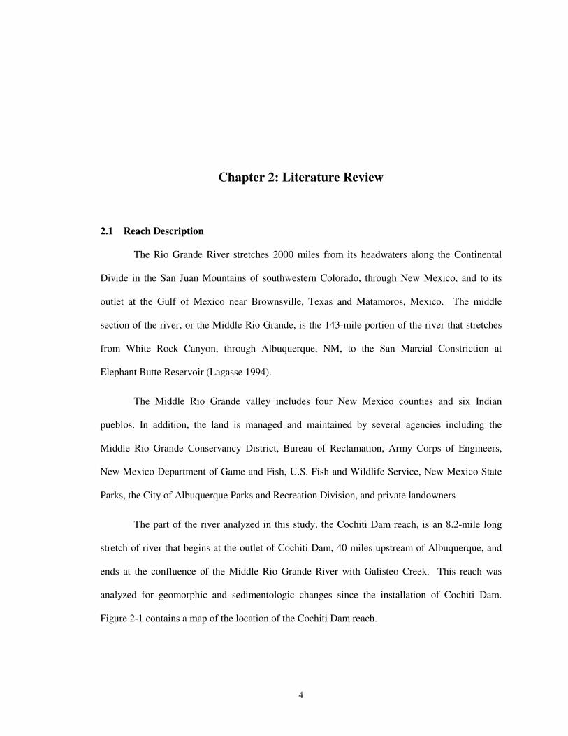
The part of the river analyzed in this study, the Cochiti Dam reach, is an 8.2-mile long
stretch of river that begins at the outlet of Cochiti Dam, 40 miles upstream of Albuquerque, and
ends at the confluence of the Middle Rio Grande River with Galisteo Creek. This reach was
analyzed for geomorphic and sedimentologic changes since the installation of Cochiti Dam.
Figure 2-1 contains a map of the location of the Cochiti Dam reach.
5
�Figure 2-1 Cochiti Dam reach topographical map and location map
6
2.2 Middle Rio Grande History
The Middle Rio Grande valley has been cultivated for hundreds of years. The earliest
Pueblo (Anasazi) Indian villages date back to the 1300’s (Scurlock 1998) and consisted of over
25,000 acres of farmland with hand-dug irrigation ditches from the Rio Grande. Spanish
explorers conquered the land in the early 1500’s, led by Coronado (Burkholder 1929, Crawford et
al. 1993). In the 1800’s, white settlers began to farm the area as well. Irrigated lands reached a
maximum area of 124,000 acres of land by 1880 (Lagasse 1980). The agricultural area was
reduced thereafter due to the rising water table and strains on water supply.
The heavy agricultural use by farmers and ranchers in Colorado reduced the water quality
received by New Mexico farmers. The overall flow was reduced and became laden with
agricultural pollutants and erosion-induced sediment. In addition, arroyo cutting began in the late
1800’s, increasing upland erosion (Hereford 1984). The sediment transport capacity of the river
was reduced with the decreasing flow, and the bed began to aggrade. Aggradation of the bed
caused seepage and an increase in water table elevation. The river became very shallow and wide
with a high susceptibility to flooding (Burkholder 1929). The agricultural lands along the river
experienced flooding, waterlogged land, and failed irrigation systems (Scurlock 1998). By 1925,
irrigated agricultural area still in use was reduced to 40,000 acres (Leon 1998).
During the early 1900’s, the US Congress commissioned a series of dams, levees,
diversion structures, and channelization works during the Rio Grande Reclamation Project. A
component of this project, Elephant Butte Dam, was completed in 1915. This dam is the
principal storage facility for the Rio Grande-Chama Project, which delivers water for downstream
use under contract between the USBR and the Elephant Butte Irrigation District in New Mexico
and the El Paso County Water Improvement District #1 in Texas. It is operated to ensure that
60,000 acre-feet per year of water is delivered to the Aceuia Madre headgate in Mexico, in
accordance with the U.S. 1906 Treaty with Mexico (USACE 2005).
7
The Middle Rio Grande Conservancy District (MRGCD) was organized in 1925 to
improve drainage, irrigation, and flood control for 128,000 acres of land, including urban areas,
in the Middle Rio Grande region. Flood control and sediment detention works were established
in the early 1930’s. The Middle Rio Grande Floodway was constructed in 1935 (Woodson 1961).
It was designed with an average width of 1500 feet (between levees), and 8-foot-high levees.
Design flow for the floodway was 40,000 cfs. The floodway levee heights were increased in
Albuquerque to accommodate a passing design flow of 75,000 cfs (Woodson and Martin 1962).
In addition to the numerous drainage canals, main irrigation canals, and two canal
headings, the MRGCD is responsible for the building, operation, and maintenance of the El Vado
Dam on the Rio Chama, Angostura Dam, Isleta Dam, San Acacia Dam, and Cochiti Dam
(Lagasse 1980).
In 1948, as the result of a highly damaging flood, the USACE and the USBR together
with various other Federal, State, and local agencies proposed the Comprehensive Plan of
Improvement for the Rio Grande in New Mexico (Pemberton 1964). Aggradation and seepage
leading to floodway deterioration indicated the need for the regulation of floodflows, sediment
retention, and channel stabilization (Woodson and Martin 1963). The Comprehensive Plan
included plans for a system of reservoirs (Abiquiu, Jemez, Cochiti, Galisteo) on the Rio Grande
and its tributaries, along with floodway rehabilitation (Woodson and Martin 1962). This reduced
the floodway capacity to 20,000 cfs with a reduction to 42,000 cfs in Albuquerque (Leon 1998).
The reservoirs were built by the USACE and the floodway rehabilitation was done by the
USACE and the USBR (Woodson and Martin 1963).
Cochiti Dam on the Middle Rio Grande and Galisteo Dam on Galisteo Creek were both
authorized in 1960 by the USACE (Woodson and Martin 1963). Cochiti Dam was built chiefly
for flood and sediment control. An initial 50,000 acre-feet of San Juan-Chama Project water was
released for the original filling of a pool of 1200 acres of surface area in Cochiti Reservoir
8
USACE 2005) and continues to maintain an average of 50,000 acre-feet behind Cochiti Dam for
recreational purposes. Trap efficiency for Cochiti Reservoir is estimated at 87% by the USACE
(USACE 2005). Trapping of the sediment prevented continued aggradation of the reach and
began clearwater scour (Lagasse 1980). Bed material coarsening was expected as far downstream
as the Rio Puerco confluence, preventing excessive degradation (Sixta 2004).
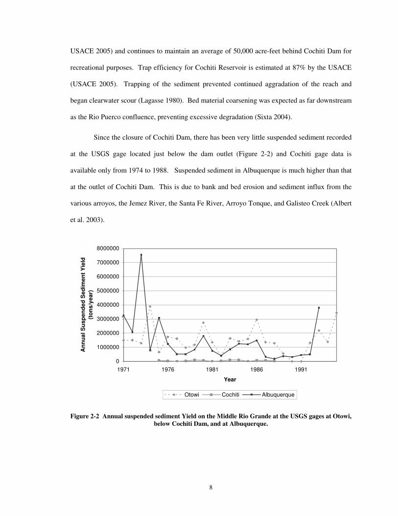
Since the closure of Cochiti Dam, there has been very little suspended sediment recorded
at the USGS gage located just below the dam outlet (Figure 2-2) and Cochiti gage data is
available only from 1974 to 1988. Suspended sediment in Albuquerque is much higher than that
at the outlet of Cochiti Dam. This is due to bank and bed erosion and sediment influx from the
various arroyos, the Jemez River, the Santa Fe River, Arroyo Tonque, and Galisteo Creek (Albert
et al. 2003).
0
1000000
2000000
3000000
4000000
5000000
6000000
7000000
8000000
1971 1976 1981 1986 1991
Year
Ann
ual S
uspe
nded
Sed
imen
t Yie
ld
(ton
s/ye
ar)
Otowi Cochiti Albuquerque�
Figure 2-2 Annual suspended sediment Yield on the Middle Rio Grande at the USGS gages at Otowi, below Cochiti Dam, and at Albuquerque.
9
Cochiti Reservoir is located within the boundaries of the Pueblo de Cochiti Nation. The
native peoples living in the Cochiti Dam reach did not welcome the plans for Cochiti Dam
because of the potential damage to their cultural, agricultural, economical, and political life. As a
result of the dam’s construction, the Pueblo people endured structural testing that led to the flood
of their agricultural land and a resulting twenty year loss of farming and way of life. In 2001,
after lengthy lawsuits and victories for the Pueblo people, the USACE gave a public apology and
cooperative efforts have been maintained since (Pueblo de Cochiti Web site 2005). Data on the
Pueblo de Cochiti Nation, however, is very difficult to obtain and was sometimes not taken at all.
2.3 Hydrology, Geology, and Climate of the Middle Rio Grande
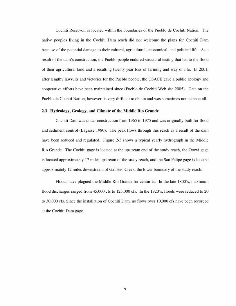
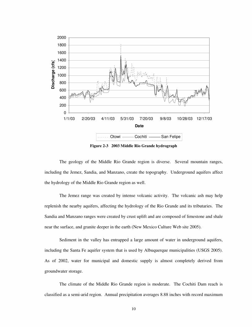
Cochiti Dam was under construction from 1965 to 1975 and was originally built for flood
and sediment control (Lagasse 1980). The peak flows through this reach as a result of the dam
have been reduced and regulated. Figure 2-3 shows a typical yearly hydrograph in the Middle
Rio Grande. The Cochiti gage is located at the upstream end of the study reach, the Otowi gage
is located approximately 17 miles upstream of the study reach, and the San Felipe gage is located
approximately 12 miles downstream of Galisteo Creek, the lower boundary of the study reach.
Floods have plagued the Middle Rio Grande for centuries. In the late 1800’s, maximum
flood discharges ranged from 45,000 cfs to 125,000 cfs. In the 1920’s, floods were reduced to 20
to 30,000 cfs. Since the installation of Cochiti Dam, no flows over 10,000 cfs have been recorded
at the Cochiti Dam gage.
10
0
200
400
600
800
1000
1200
1400
1600
1800
2000
1/1/03 2/20/03 4/11/03 5/31/03 7/20/03 9/8/03 10/28/03 12/17/03
Date
Dis
char
ge (c
fs)
Otowi Cochiti San Felipe�
Figure 2-3 2003 Middle Rio Grande hydrograph ��
The geology of the Middle Rio Grande region is diverse. Several mountain ranges,
including the Jemez, Sandia, and Manzano, create the topography. Underground aquifers affect
the hydrology of the Middle Rio Grande region as well.
The Jemez range was created by intense volcanic activity. The volcanic ash may help
replenish the nearby aquifers, affecting the hydrology of the Rio Grande and its tributaries. The
Sandia and Manzano ranges were created by crust uplift and are composed of limestone and shale
near the surface, and granite deeper in the earth (New Mexico Culture Web site 2005).
Sediment in the valley has entrapped a large amount of water in underground aquifers,
including the Santa Fe aquifer system that is used by Albuquerque municipalities (USGS 2005).
As of 2002, water for municipal and domestic supply is almost completely derived from
groundwater storage.
The climate of the Middle Rio Grande region is moderate. The Cochiti Dam reach is
classified as a semi-arid region. Annual precipitation averages 8.88 inches with record maximum
11
(1988) of 13.11 inches and record minimum (1989) of 4.99 inches. Mean annual temperature is
56.4 degrees Fahrenheit with a daily maximum (6/26/1994) of 107 and a daily minimum
(1/07/1971) of -17 degrees. More than 90 percent of New Mexico’s precipitation returns to the
atmosphere through evapotranspiration due to the warm, dry climate and high winds (USBR
2005).
The hot dry climate makes loss rates for the Middle Rio Grande fairly high. From Otowi
to Cochiti Dam, 0.33 % of water is lost to evaporation, storage, and seepage into the banks. Flow
takes three days to travel from Cochiti Dam to Elephant Butte Reservoir and can have water loss
of anywhere from 3.3% in the winter to 7.2% in the summer (USACE 2005).
2.4 Previous Studies of the Middle Rio Grande
The Middle Rio Grande is one of the most historically documented rivers in the US (Graf
1994). Numerous studies on the changes to the Middle Rio Grande have been done to estimate
river bed and planform configurations, geometry patterns, bed material characteristics, and future
conditions. Research has been done on the changes to the river as a result of agriculture,
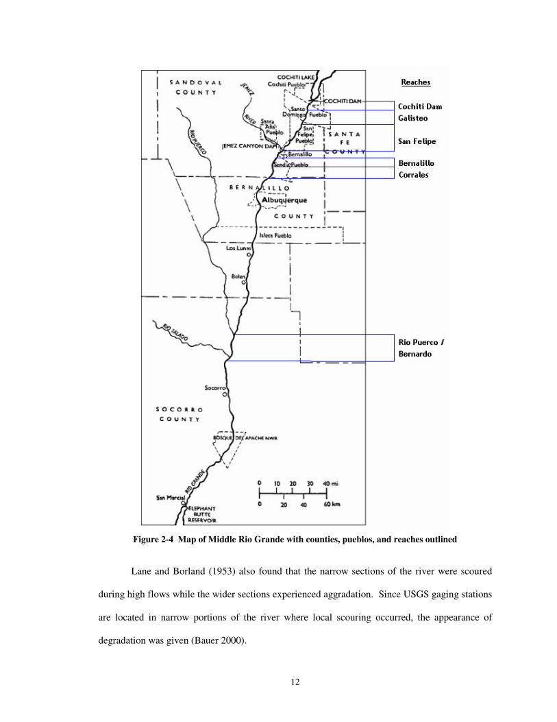
channelization, levees, dams and restoration techniques. Figure 2-4 outlines the locations of
reaches and tributaries in the Middle Rio Grande.
Nordin and Beverage (1965) describe the pre-Cochiti Dam river below Cochiti Pueblo to
be a wide, unconfined, braided channel with many coarse gravel and cobble islands. During low-
flow, the riverbed was mostly sand, and during high flows the bed was mostly gravel. Below the
mouth of the Jemez River the Rio Grande was a sand bed river. Lane and Borland (1953) had a
similar assessment of the dam, noting that the river did not have the bends and crossings that are
generally found in other large alluvial rivers.
�
�
�
12
�Figure 2-4 Map of Middle Rio Grande with counties, pueblos, and reaches outlined
Lane and Borland (1953) also found that the narrow sections of the river were scoured
during high flows while the wider sections experienced aggradation. Since USGS gaging stations
are located in narrow portions of the river where local scouring occurred, the appearance of
degradation was given (Bauer 2000).
13
Studies were done to estimate aggradational and degradational trends to the river after the
construction of the dams. Woodson and Martin (1962) estimated that the system of reservoirs
(Abiquiu, Jemez, Galisteo, and Cochti) would reduce the sediment inflow into Bernalillo by 75
percent after 20 years. They also expected degradation to begin at Cochiti Dam and to progress
downstream as far as the Rio Puerco. Due to bed armoring, this degradation was not expected to
exceed 3 feet. The USBR also estimated that degradation would begin by 1965 and the river
would experience no more than 1 foot of aggradation by 1985 (Schembera 1962).
Within two months after the Cochiti Dam closure in 1973, observers noted that the first
three miles below the dam were lacking bed material sizes smaller than 1 mm. Gravel bars began
appearing as far downstream as Albuquerque (Dewey et al. 1979). Bed material surveys taken in
the early 1970’s indicated the median grain size for much of the reach was less than 1 mm. By
1995, the median grain size had increased to over 10 mm. The coarsening of the bed had
progressed downstream over 28 miles below Cochiti Dam (Dewey et al. 1979, Bauer 2000).
Lagasse (1980) performed a geomorphic analysis of the Middle Rio Grande from Cochiti
Dam to the Isleta Diversion Dam for the time period from 1971 to 1975. This study concluded
that the water and sediment influx from arroyos and tributaries have dominated the river’s
response to the dam construction (Leon 1998). After the dam closure, Lagasse calculated a zone
of channel incision and bed coarsening, which migrated rapidly downstream at a rate of 5
km/year. After 1980, it slowed to an average of 0.7 km/year (Ortiz and Meyer 2005). Stable
conditions were approached sooner above the confluence of the middle Rio Grande with the
Jemez River than downstream due to armoring and stable tributary base levels (Leon 1998). Just
upstream of the Isleta Diversion Dam, Lagasse (1980) found the bed had aggraded, indicating
large amounts of sediment load transport from upstream in the reach (Bauer 2000). Lagasse’s
analysis was documented through a qualitatative analysis of planform, profile, cross-section and
sediment data (Leon 1998). Lagasse’s methodology has been used as a guide for this study.
14
Leon’s 1998 study of the river from Cochiti Dam to Bernalillo Bridge found similar
results to Lagasse’s (1980) report. A degradational trend was noted with the maximum
degradation occurring at the downstream end of the reach. Degradation of up to 8 feet was
observed between 1971 and 1995.
Graf (1998) studied plutonium transport into the Northern Rio Grande. He documented
channel changes based on 1940 to 1980 aerial photos and topographical maps. The photos
indicated that the river had a shallow, wide, braided planform before 1940. After implementation
of the Comprehensive Plan of Improvement, flows decreased and the channel narrowed
throughout most of the Middle Rio Grande reach. The floodplain increased and the river
transitioned from a braided planform to a single-thread channel (Bauer 2000). This transition
may be due to dam closures or regional hydroclimatic influences since the river upstream of
Cochiti Dam has also narrowed and tended towards a single thread channel since the 1940s. With
the narrowing of the channel came instability and higher rates of lateral migration. The main
channel of the Middle Rio Grande changed position by as much as 1 km (0.6 miles) between
1940 and 1980. These changes occurred during high flows when sediment blocked the main flow
path and forced channel avulsions (Graf 1994).
The reduced peak flows have also complicated the hydraulics at the tributary confluences
to the Rio Grande (Bauer 2000). The sediment transported by these tributaries frequently exceeds
the rivers capacity to transport the sediment (Crawford et al. 1993). Complications from
occurrence can be seen at the mouth of the Rio Puerco. The Rio Puerco is not as stable as the Rio
Grande due to constant aggradation and channel cutting that has occurred over the past 3000
years, cutting and filling at least three major channels. This process is a result of varying
sediment fluxes to the Rio Grande (Crawford et al. 1993). The sediment transported through the
Rio Grande due to bed degradation is estimated to be 65% of the total sediment passing the
Albuquerque and Bernardo gages. However, downstream at the San Acacia and San Marcial
15
gages, the majority of the transported sediment passing the gage is supplied by the Rio Puerco
with the degradation of the bed contributing less than 8% of the sediment downstream of the Rio
Puerco (Albert 2004). The Rio Puerco currently contributes twice the sediment through its
channel than what is carried through the Rio Grande in Albuquerque. This sediment is deposited
upstream of the San Marcial gaging station (Bauer 2000).
Sanchez and Baird (1997) studied morphologic changes to the river since 1918. A
narrowing trend was observed that did not accelerate after the completion of Cochiti Dam. The
sinuosity of the river increased after dam construction, but did not reach the peak value observed
in 1949. The historical bankfull discharge of 11,166 cfs has never been released from Cochiti
Dam. Due to flow regulation at the dam, the two-year return flow has been reduced to 5650 cfs.
According to Sanchez and Baird’s study, the channelization works, dam construction, and
regulated flows together account for the overall channel narrowing that has occurred since the
1940’s.
Mosley and Boelman (1998) studied the Santa Ana, located between the Angostura
Diversion Dam and the Highway 44 Bridge in Bernalillo. Their study concluded that the reach
altered its planform from braided to a meandering riffle/pool pattern, the bed material size
increased to gravel, and the width to depth ratio decreased since dam construction (Sixta 2004).
Similar findings were reported by Ortiz and Meyer (2005), who studied changes to the
river just downstream of Bernalillo Bridge. They characterized the pre-dam channel as having a
multi-thalweg, shallow, bar-braided planform, with uniform channel width due to bank
stabilization structures and associated dense vegetation. Post-dam conditions included an
increase in vegetated island surface area, widespread thalweg incision, and a disconnected
floodplain throughout the reach, due to the regime of reduced peak discharges.
Several other studies have been funded by the USBR on the morphology of the Middle
Rio Grande. The research conducted for these reports was performed at Colorado State
16
University under the guidance of Dr. P. Y. Julien. The following reaches have been investigated
as of 2005:
Rio Puerco (Richard et al. 2001). This is the downstream-most reach studied, spanning
10 miles from the mouth of the Rio Puerco (agg/deg 1101, river mile 126) to the San Acacia
Diversion Dam (agg/deg 1206, river mile 116.2).
Corrales (Leon and Julien, 2001a), updated by Albert et al. (2003). This reach spans 10.3
miles from the Corrales Flood Channel (agg/deg 351, river mile 196) to the Montano Bridge
(agg/deg 462, river mile 188)
• Bernalillo Bridge (Leon and Julien 2001b), updated by Sixta et al. (2003a). This reach
spans 5.1 miles from New Mexico Highway 44 (agg/deg 298, river mile 203.8) to cross-
section CO-33 (agg/deg351, river mile 198.2).
• San Felipe (Sixta et al. 2003b). This reach spans 6.2 miles from the mouth of Arroyo
Tonque (agg/deg 174, river mile 217) to the Angostura Diversion Dam (agg/deg 236,
river mile 209.7).
• Cochiti Dam (Novak 2005 draft). This reach spans 8.2 miles from the outlet of Cochiti
Dam (agg/deg 17, river mile 232.6) to the mouth of Galisteo Creek (agg/deg 97, river
mile 224.4).�
The vast research done on the Middle Rio Grande at CSU under Dr. P. Y. Julien over the
past several years has prompted the creation of the Middle Rio Grande Database. The database
includes all data, analysis and literature pertaining to these studies. The database was updated in
2004 to include all theses and dissertations, as well as all USBR reports for completeness.
Appendix G contains a summary of the updating of the Middle Rio Grande Database.
��
17
�
�
�
�
�
Chapter 3: Geomorphic Characterization
Understanding the historical spatial and temporal trends in the Cochiti Dam reach is a
crucial step in developing habitat restoration plans for the Rio Grande silvery minnow and the
southwestern willow flycatcher. The objective of this chapter was to identify and quantify
changes and trends in the channel geometry, discharge, and sediment characteristics.
To achieve this objective, the following tasks will be addressed:
• Analysis of spatial and temporal trends in channel geometry through inspection
of cross-section survey data.
• Channel planform classification through analysis of aerial photos, topographic
maps, and digitized planforms.
• Identification of spatial and temporal trends in water and sediment discharge and
concentration using USGS gaging station data.
3.1 Site Description and Background
The 8.2-mile-long Cochiti Dam Reach of the middle Rio Grande stretches from Cochiti
Dam (river mile 232.6) to the confluence with Galisteo Creek (river mile 224.6). The reach
meanders slightly with an average sinuosity between 1.1 and 1.2. The reach has an average
valley slope of 0.0016. The median bed material in the channel reach is coarse gravel, with a
sediment distribution ranging from fine sand to small cobbles.
18
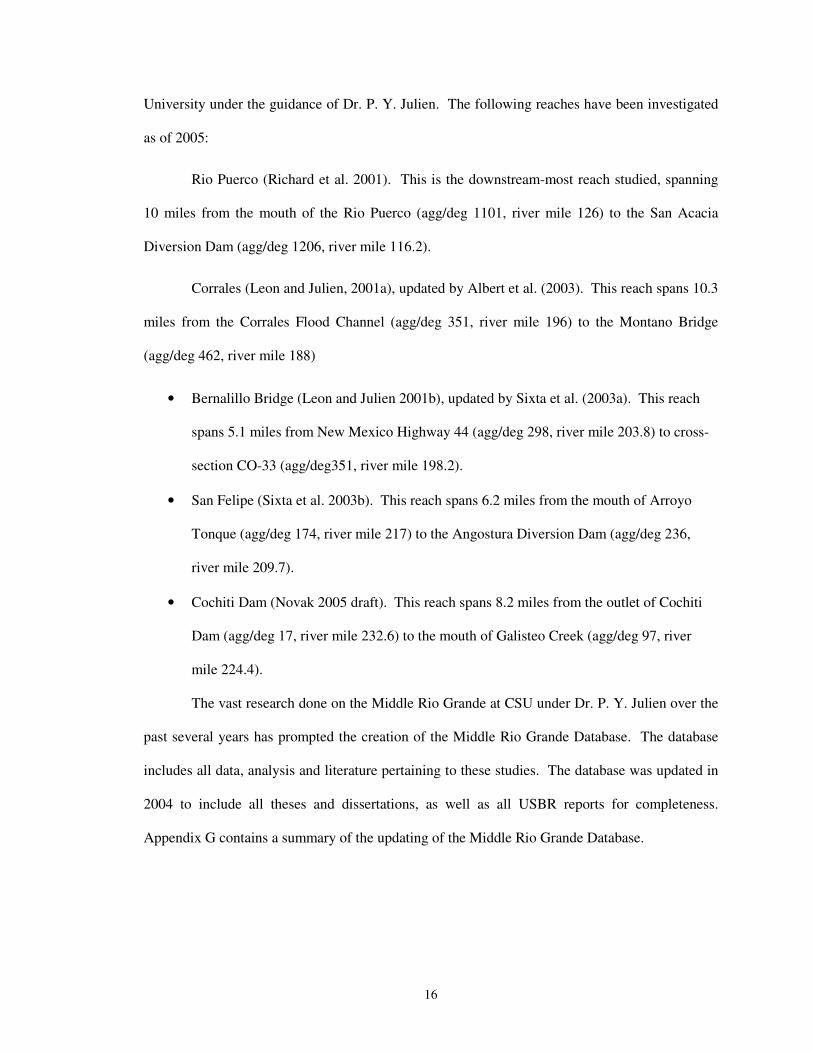
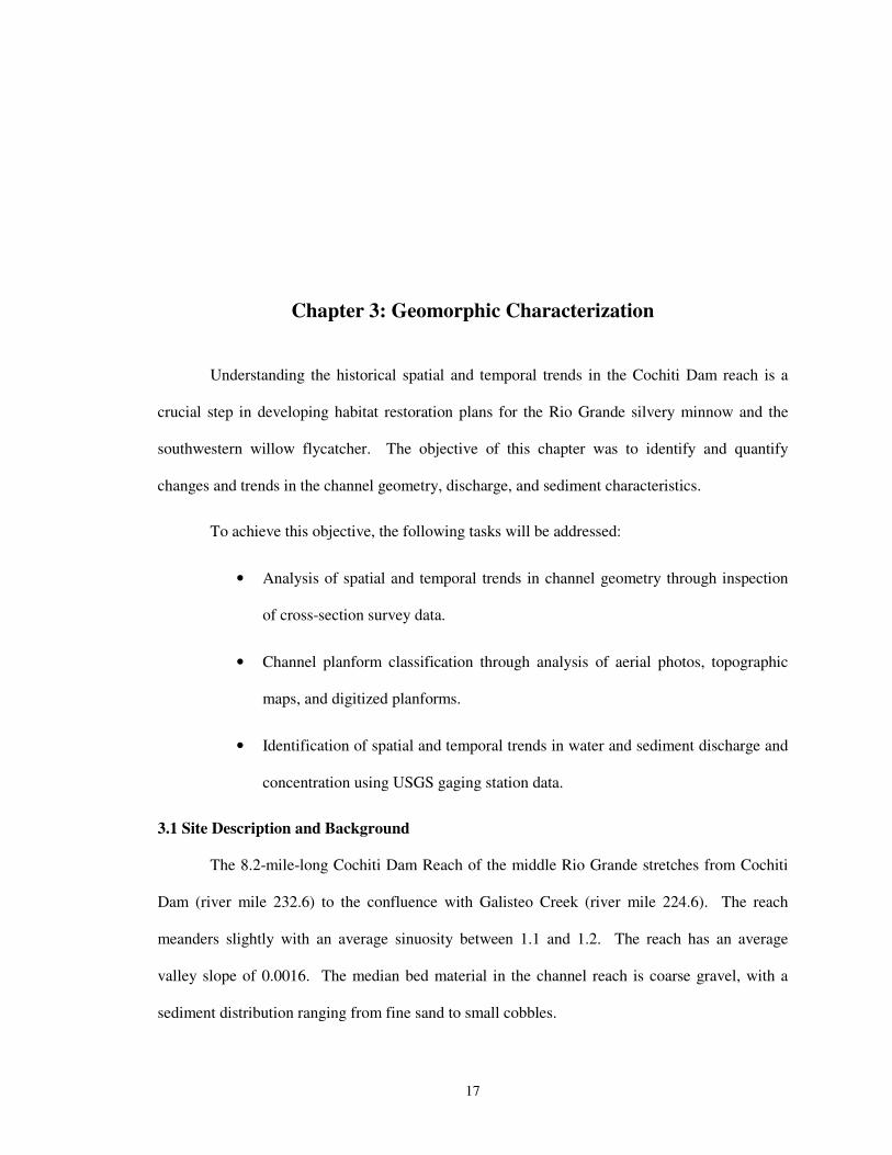
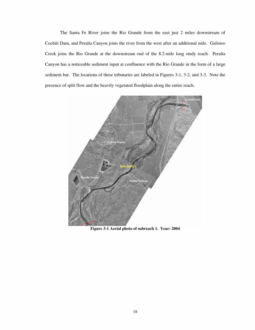
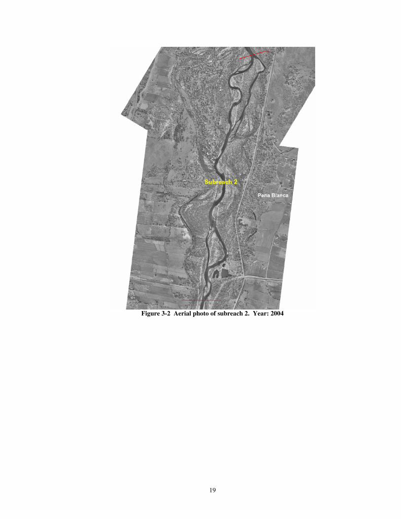
The Santa Fe River joins the Rio Grande from the east just 2 miles downstream of
Cochiti Dam, and Peralta Canyon joins the river from the west after an additional mile. Galisteo
Creek joins the Rio Grande at the downstream end of the 8.2-mile long study reach. Peralta
Canyon has a noticeable sediment input at confluence with the Rio Grande in the form of a large
sediment bar. The locations of these tributaries are labeled in Figures 3-1, 3-2, and 3-3. Note the
presence of split flow and the heavily vegetated floodplain along the entire reach.
�Figure 3-1 Aerial photo of subreach 1. Year: 2004
�
19
�Figure 3-2 Aerial photo of subreach 2. Year: 2004
20
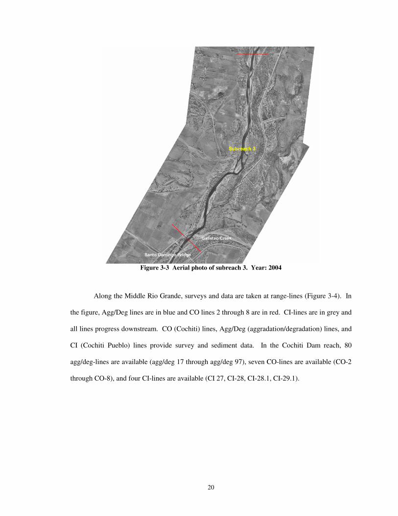
�Figure 3-3 Aerial photo of subreach 3. Year: 2004
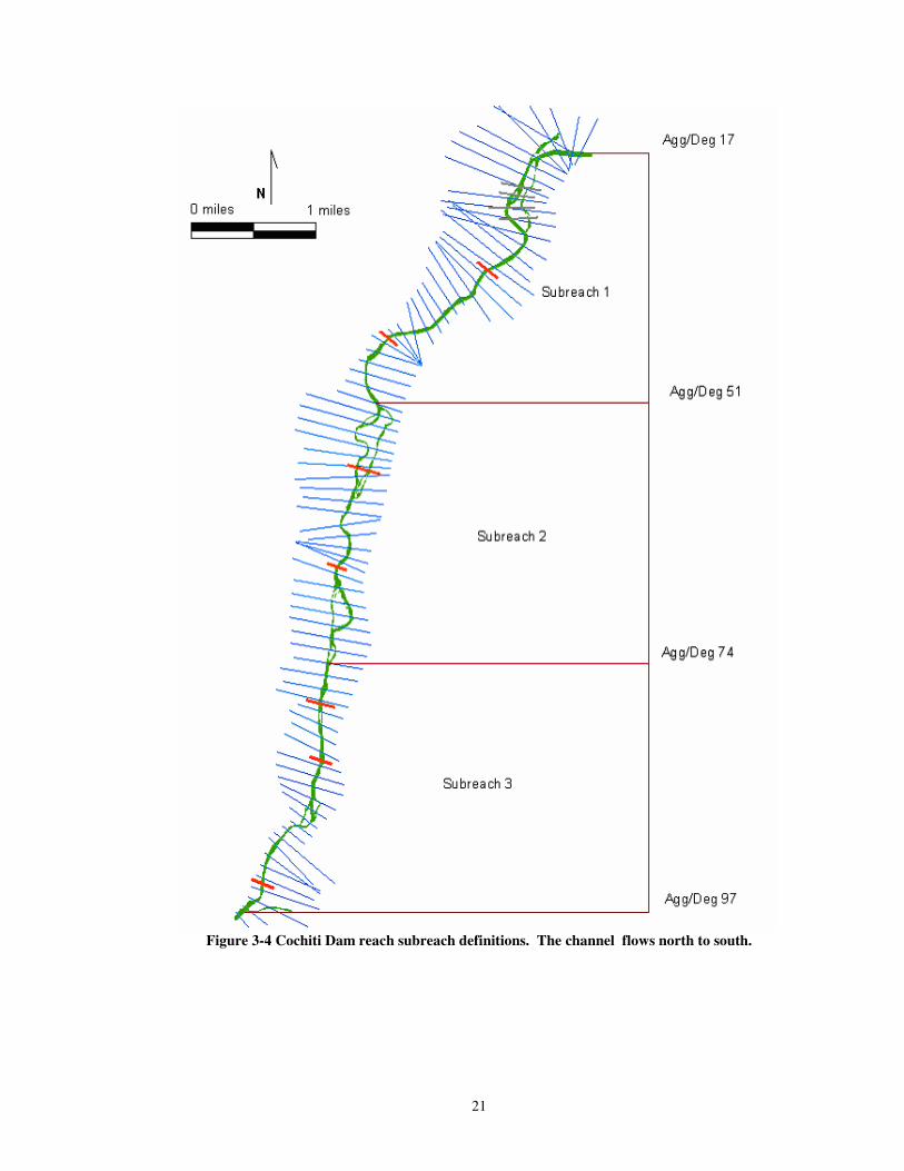
Along the Middle Rio Grande, surveys and data are taken at range-lines (Figure 3-4). In
the figure, Agg/Deg lines are in blue and CO lines 2 through 8 are in red. CI-lines are in grey and
all lines progress downstream. CO (Cochiti) lines, Agg/Deg (aggradation/degradation) lines, and
CI (Cochiti Pueblo) lines provide survey and sediment data. In the Cochiti Dam reach, 80
agg/deg-lines are available (agg/deg 17 through agg/deg 97), seven CO-lines are available (CO-2
through CO-8), and four CI-lines are available (CI 27, CI-28, CI-28.1, CI-29.1).
�
21
�Figure 3-4 Cochiti Dam reach subreach definitions. The channel flows north to south.
22
3.1.1 Subreach Definition
The Cochiti Dam reach of the middle Rio Grande was subdivided into three subreaches to
facilitate geomorphic and sedimentologic analysis. The subreaches were chosen based on
characteristic similarities such as planform, width, and sinuosity. Subreach 1 is 2.54 miles long
and stretches from agg/deg line 17 to 51; subreach 2 is 2.14 miles long and runs from agg/deg
line 51 to 74, and subreach 3, 2.11 miles long, runs from agg/deg line 74 to 95. Agg/deg line 95
is located immediately at the mouth of Galisteo Creek, just upstream of Santo Domingo Bridge.
The subreaches are defined in Figure 3-4.
3.1.2 Available Data
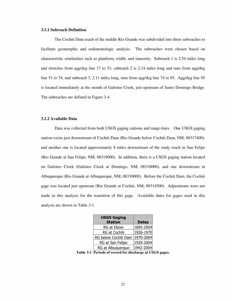
Data was collected from both USGS gaging stations and range-lines. One USGS gaging
station exists just downstream of Cochiti Dam (Rio Grande below Cochiti Dam, NM, 08317400),
and another one is located approximately 8 miles downstream of the study reach in San Felipe
(Rio Grande at San Felipe, NM, 08319000). In addition, there is a USGS gaging station located
on Galisteo Creek (Galisteo Creek at Domingo, NM, 08318000), and one downstream in
Albuquerque (Rio Grande at Albuquerque, NM, 08330000). Before the Cochiti Dam, the Cochiti
gage was located just upstream (Rio Grande at Cochiti, NM, 08314500). Adjustments were not
made in this analysis for the transition of this gage. Available dates for gages used in this
analysis are shown in Table 3-1.
������������
����� ��� �
����������� �� ������
������������ ��������
������������������� ���������
���������������� � �������
������!��"#"�$#"�� ���������Table 3-1 Periods of record for discharge at USGS gages.
�
23
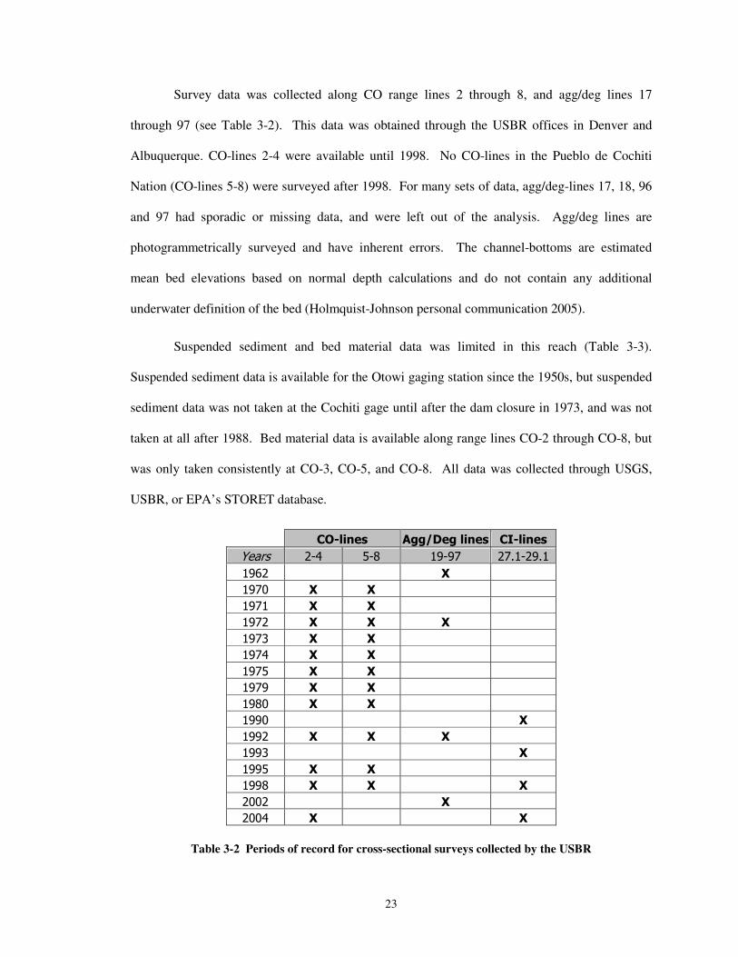
Survey data was collected along CO range lines 2 through 8, and agg/deg lines 17
through 97 (see Table 3-2). This data was obtained through the USBR offices in Denver and
Albuquerque. CO-lines 2-4 were available until 1998. No CO-lines in the Pueblo de Cochiti
Nation (CO-lines 5-8) were surveyed after 1998. For many sets of data, agg/deg-lines 17, 18, 96
and 97 had sporadic or missing data, and were left out of the analysis. Agg/deg lines are
photogrammetrically surveyed and have inherent errors. The channel-bottoms are estimated
mean bed elevations based on normal depth calculations and do not contain any additional
underwater definition of the bed (Holmquist-Johnson personal communication 2005).
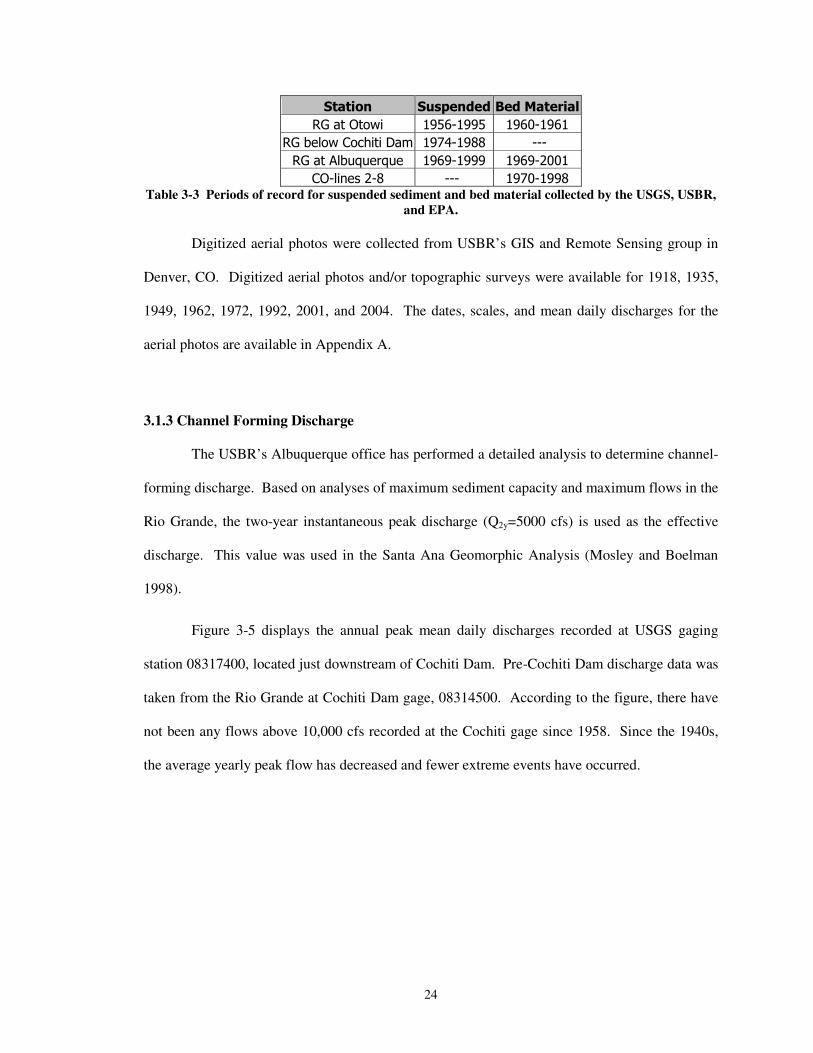
Suspended sediment and bed material data was limited in this reach (Table 3-3).
Suspended sediment data is available for the Otowi gaging station since the 1950s, but suspended
sediment data was not taken at the Cochiti gage until after the dam closure in 1973, and was not
taken at all after 1988. Bed material data is available along range lines CO-2 through CO-8, but
was only taken consistently at CO-3, CO-5, and CO-8. All data was collected through USGS,
USBR, or EPA’s STORET database.
�� ������� � ������������ � ������� �
%��$&� ���� ��� ����� ��'���'�
���� �� �� �� ��
���� �� �� �� ��
��� �� �� �� ��
���� �� �� �� ��
�� � �� �� �� ��
���� �� �� �� ��
�� � �� �� �� ��
���� �� �� �� ��
���� �� �� �� ��
���� �� �� �� ��
���� �� �� �� ��
�� � �� �� �� ��
�� � �� �� �� ��
���� �� �� �� ��
����� �� �� �� ��
����� �� �� �� ��
�Table 3-2 Periods of record for cross-sectional surveys collected by the USBR
24
����� �� �������������������
����������� � ���� � �������
������������������� �������� �����
������!��"#"�$#"�� �������� ��������
������&����� ����� ��������Table 3-3 Periods of record for suspended sediment and bed material collected by the USGS, USBR,
and EPA. �
Digitized aerial photos were collected from USBR’s GIS and Remote Sensing group in
Denver, CO. Digitized aerial photos and/or topographic surveys were available for 1918, 1935,
1949, 1962, 1972, 1992, 2001, and 2004. The dates, scales, and mean daily discharges for the
aerial photos are available in Appendix A.
�
3.1.3 Channel Forming Discharge
The USBR’s Albuquerque office has performed a detailed analysis to determine channel-
forming discharge. Based on analyses of maximum sediment capacity and maximum flows in the
Rio Grande, the two-year instantaneous peak discharge (Q2y=5000 cfs) is used as the effective
discharge. This value was used in the Santa Ana Geomorphic Analysis (Mosley and Boelman
1998).
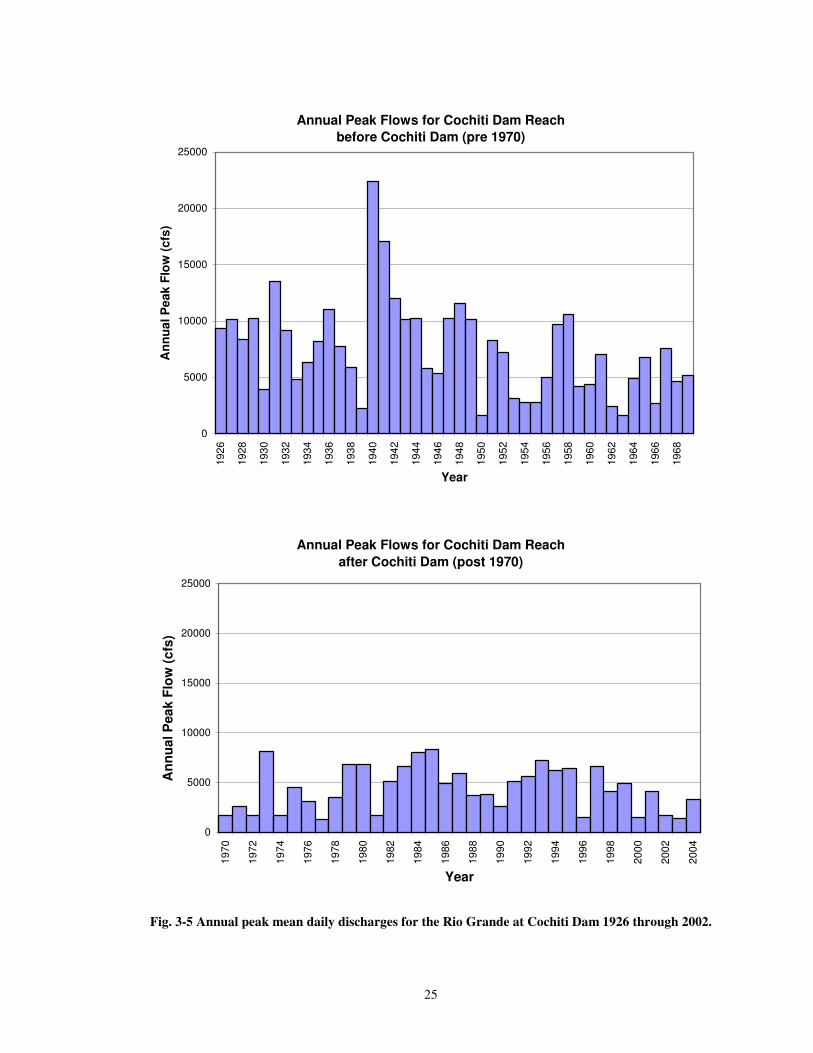
Figure 3-5 displays the annual peak mean daily discharges recorded at USGS gaging
station 08317400, located just downstream of Cochiti Dam. Pre-Cochiti Dam discharge data was
taken from the Rio Grande at Cochiti Dam gage, 08314500. According to the figure, there have
not been any flows above 10,000 cfs recorded at the Cochiti gage since 1958. Since the 1940s,
the average yearly peak flow has decreased and fewer extreme events have occurred.
�
25
Annual Peak Flows for Cochiti Dam Reach before Cochiti Dam (pre 1970)
0
5000
10000
15000
20000
25000
1926
1928
1930
1932
1934
1936
1938
1940
1942
1944
1946
1948
1950
1952
1954
1956
1958
1960
1962
1964
1966
1968
Year
Ann
ual P
eak
Flow
(cfs
)
Annual Peak Flows for Cochiti Dam Reach after Cochiti Dam (post 1970)
0
5000
10000
15000
20000
25000
1970
1972
1974
1976
1978
1980
1982
1984
1986
1988
1990
1992
1994
1996
1998
2000
2002
2004
Year
Ann
ual P
eak
Flow
(cfs
)
Fig. 3-5 Annual peak mean daily discharges for the Rio Grande at Cochiti Dam 1926 through 2002.�
26
3.2 Methods
3.2.1 Channel Classification
The channel reach was classified using aerial photos from 2002. Geographic Information
System (GIS) coverages ranging from 1918 to 2004 of the historical active channel were used to
qualitatively describe the non-vegetated channel planform. The determination of channel
classification for the Cochiti Dam reach was done using several different methods, discussed
below:
Slope-discharge relationships were applied using methods devised by Leopold and
Wolman (1957), Lane (1957, from Richardson et al. 1990), Henderson (1963, from Henderson
1966), Ackers and Charlton (1970, from Ackers 1982) and Schumm and Kahn (1972). Channel
morphology methods were implemented from Rosgen (1994).
In addition, channel classifications based on stream-power were calculated using methods
by Chang (1979), Van den Berg (1995), Knighton and Nanson (1993), and Nanson and Croke
(1992). Finally, Parker’s (1976) method of stream classification was used, which employs
slope/Froude number and flow depth/flow width.
Slope-Discharge methods:
Leopold and Wolman (1957) classify channel planforms as meandering, braided, or
straight. Slope-discharge relationships provide the criterion upon which these classifications are
based. Braided and meandering channels are separated by the following equation:
So =0.06Q -0.44,
where Q is the bankfull discharge in cfs and So is the channel bedslope in ft/ft. Leopold
and Wolman refer to meandering rivers as those with a sinuosity greater than 1.5. Channels with
relatively stable alluvial islands are refered to as braided. All units are English.
27
Lane (1957, from Richardson et al. 1990) proposed a relationship for sand bed channels
based on a dimensionless parameter, K:
SoQ 0.25=K,
where So is in ft/ft and Q is in cfs. The channel classification is then determined using
the following criteria:
K � 0.0017 meandering
0.0017 < K < 0.010 intermediate (transitional)
K � 0.010 braided
All units are English.
Henderson (1963, from Henderson 1966) began with Leopold and Wolman’s slope-
discharge relationship, and added a bed material factor, d, which describes the median grain size
in feet. Plotting So/0.06Q -0.44 against d empirically derived the following relationship:
So = 0.64d 1.14Q -0.44
According to Henderson, two-thirds of the channels with meandering or straight patterns
had values of S that fall close to this line. Braided channels had values of S that were much
higher than the line. Q is in cfs and So is in ft/ft. All units are English.
Ackers and Charlton (1979, Ackers 1982) developed a relationship that would distinguish
a meandering channel from a straight channel or straight channel with alternating bars.
• Sw< 0.001Q-0.12 straight channel
• 0.001Q-0.12<Sw<0.0014Q-0.12 straight channel with alternating bars
• Sv>0.0014Q-0.12 meandering channel
28
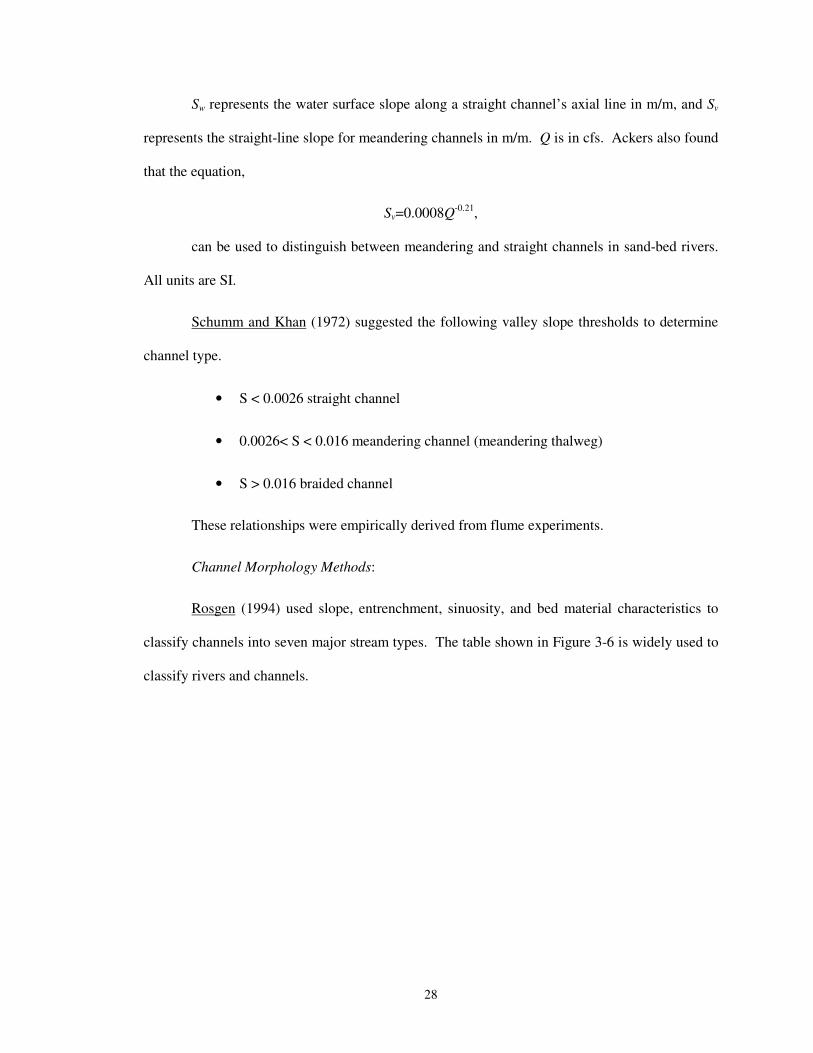
Sw represents the water surface slope along a straight channel’s axial line in m/m, and Sv
represents the straight-line slope for meandering channels in m/m. Q is in cfs. Ackers also found
that the equation,
Sv=0.0008Q-0.21,
can be used to distinguish between meandering and straight channels in sand-bed rivers.
All units are SI.
Schumm and Khan (1972) suggested the following valley slope thresholds to determine
channel type.
• S < 0.0026 straight channel
• 0.0026< S < 0.016 meandering channel (meandering thalweg)
• S > 0.016 braided channel
These relationships were empirically derived from flume experiments.
Channel Morphology Methods:
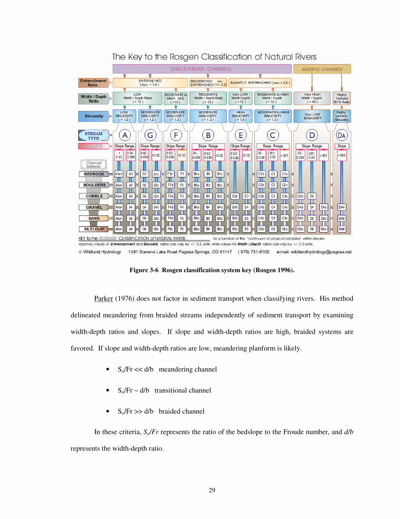
Rosgen (1994) used slope, entrenchment, sinuosity, and bed material characteristics to
classify channels into seven major stream types. The table shown in Figure 3-6 is widely used to
classify rivers and channels.
29
�
Figure 3-6 Rosgen classification system key (Rosgen 1996).
Parker (1976) does not factor in sediment transport when classifying rivers. His method
delineated meandering from braided streams independently of sediment transport by examining
width-depth ratios and slopes. If slope and width-depth ratios are high, braided systems are
favored. If slope and width-depth ratios are low, meandering planform is likely.
• So/Fr << d/b meandering channel
• So/Fr ~ d/b transitional channel
• So/Fr >> d/b braided channel
In these criteria, So/Fr represents the ratio of the bedslope to the Froude number, and d/b
represents the width-depth ratio.
30
Stream Power Methods:
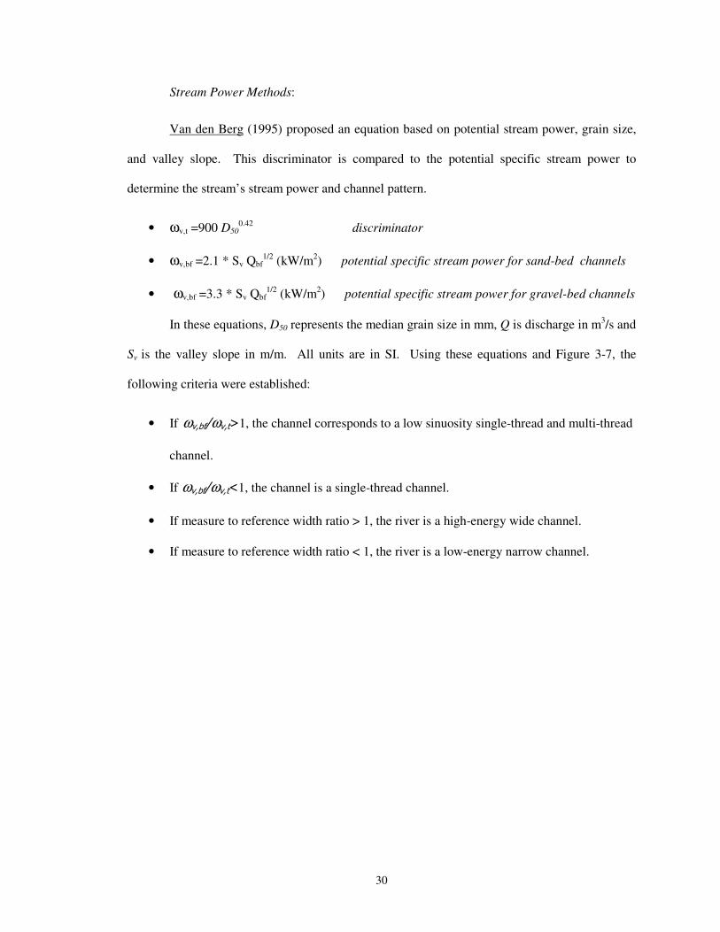
Van den Berg (1995) proposed an equation based on potential stream power, grain size,
and valley slope. This discriminator is compared to the potential specific stream power to
determine the stream’s stream power and channel pattern.
• ωv,t =900 D500.42 discriminator
• ωv,bf =2.1 * Sv Qbf1/2 (kW/m2) potential specific stream power for sand-bed channels
• ωv,bf =3.3 * Sv Qbf1/2 (kW/m2) potential specific stream power for gravel-bed channels
In these equations, D50 represents the median grain size in mm, Q is discharge in m3/s and
Sv is the valley slope in m/m. All units are in SI. Using these equations and Figure 3-7, the
following criteria were established:
• If�ω()�*+ω()�,1, the channel corresponds to a low sinuosity single-thread and multi-thread
channel.�
• If ω()�*+ω()�-1, the channel is a single-thread channel.�
• If measure to reference width ratio > 1, the river is a high-energy wide channel.
• If measure to reference width ratio < 1, the river is a low-energy narrow channel.�
�
31
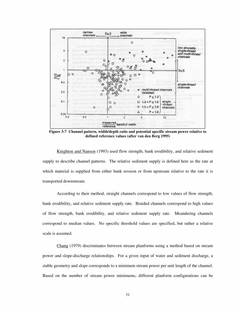
�Figure 3-7 Channel pattern, width/depth ratio and potential specific stream power relative to
defined reference values (after van den Berg 1995) ��
Knighton and Nanson (1993) used flow strength, bank erodibility, and relative sediment
supply to describe channel patterns. The relative sediment supply is defined here as the rate at
which material is supplied from either bank erosion or from upstream relative to the rate it is
transported downstream.
According to their method, straight channels correspond to low values of flow strength,
bank erodibility, and relative sediment supply rate. Braided channels correspond to high values
of flow strength, bank erodibility, and relative sediment supply rate. Meandering channels
correspond to median values. No specific threshold values are specified, but rather a relative
scale is assumed.
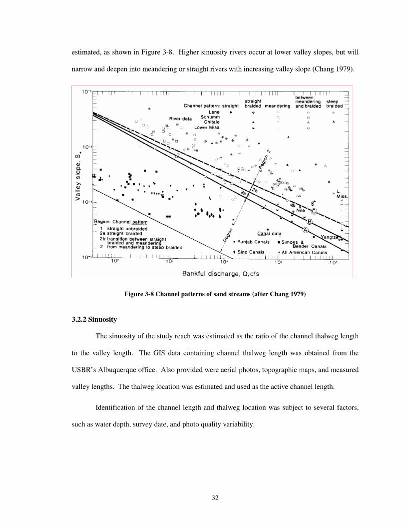
Chang (1979) discriminates between stream planforms using a method based on stream
power and slope-discharge relationships. For a given input of water and sediment discharge, a
stable geometry and slope corresponds to a minimum stream power per unit length of the channel.
Based on the number of stream power minimums, different planform configurations can be
32
estimated, as shown in Figure 3-8. Higher sinuosity rivers occur at lower valley slopes, but will
narrow and deepen into meandering or straight rivers with increasing valley slope (Chang 1979).
Figure 3-8 Channel patterns of sand streams (after Chang 1979) �
3.2.2 Sinuosity
The sinuosity of the study reach was estimated as the ratio of the channel thalweg length
to the valley length. The GIS data containing channel thalweg length was obtained from the
USBR’s Albuquerque office. Also provided were aerial photos, topographic maps, and measured
valley lengths. The thalweg location was estimated and used as the active channel length.
Identification of the channel length and thalweg location was subject to several factors,
such as water depth, survey date, and photo quality variability.
33
3.2.3 Valley Slope
The valley slope of the study reach was estimated using the agg/deg survey data. The
valley slope was computed as the ratio of valley elevation differences to the valley length. The
valley lengths were measured using GIS coverages obtained from the USBR’s GIS and Remote
Sensing Group in Denver, CO. The valley elevations were computed averages at each agg/deg
range line. Agg/deg lines are generally 400 to 600 feet apart, measuring from center to center.
The variances in this rule of thumb were taken into account throughout the analysis of this report.
3.2.4 Longitudinal Profile
Thalweg Elevation
The lowest point in each CO-line cross-section was taken to be the thalweg elevation of
the channel in that location. For the Cochiti Dam reach, thalweg data was available for CO-lines
2 through 4 from 1973 through 2004. For CO-lines 5 though 9, data was available only until
1998. CO-line surveys have not been taken in land residing in this part of the Pueblo de Cochiti
Nation since 1998. Agg/deg surveys have been taken since 1998; however, these surveys are not
detailed and give only a mean bed elevation for the channel. The changes in thalweg elevation
were plotted to show temporal trends at each location. Each CO-line cross-section for every
available date is plotted in Appendix B.
Mean Bed Elevation
The agg/deg surveys use an average bed elevation in the survey data. The cross-section
itself is not surveyed in detail. Agg/deg surveys were available for 1962, 1972, 1992, and 2002
for the 80 cross-sections in the Cochiti Dam reach. Longitudinal profiles were plotted for each
subreach, as well as for the entire reach. In addition, the subreach-averaged mean bed elevations
were calculated. Bed slope changes were measured using the differences in the average mean bed
elevation.
�
34
Friction and Water Slopes
The friction slopes were estimated at each CO-line cross-section at the channel forming
discharge mentioned in section 2.2 of 5,000 cfs. The slopes were modeled using HEC-RAS
3.1.3. The slopes were averaged over each subreach using a weighting factor. The weighting
factor was calculated as the sum of one-half of the distances to each neighboring cross-section.
An overall average slope for the entire study reach was also calculated.
3.2.5 Channel Geometry
Hydraulic Geometry
HEC-RAS 3.1.3 was used to describe the channel geometry of this reach using agg/deg
line surveys. The available 1962, 1972, 1992, and 2002 agg/deg data was modeled using the
channel forming discharge of 5,000 cfs. Seventy-six cross-sections were used in the modeling,
utilizing Agg/Deg lines 19 through 95. The cross-sections were generally spaced between 400
and 600 feet apart. These distances were measured using the digitized aerial photos in ArcGIS 9.
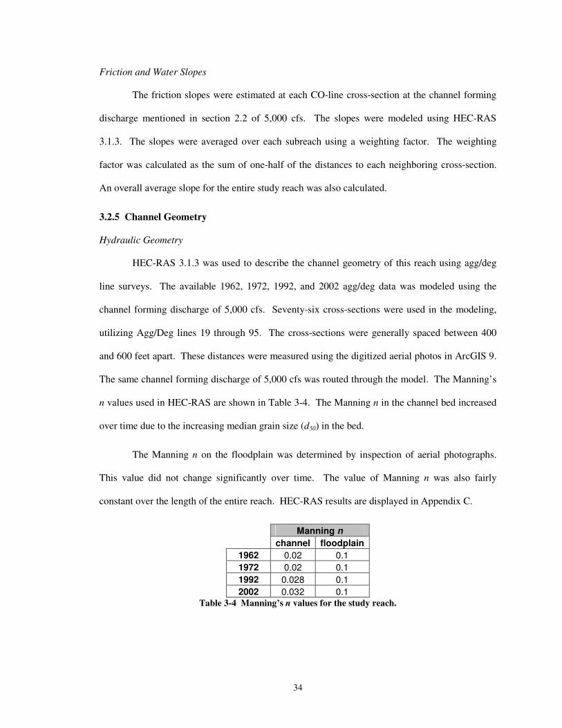
The same channel forming discharge of 5,000 cfs was routed through the model. The Manning’s
n values used in HEC-RAS are shown in Table 3-4. The Manning n in the channel bed increased
over time due to the increasing median grain size (d50) in the bed.
The Manning n on the floodplain was determined by inspection of aerial photographs.
This value did not change significantly over time. The value of Manning n was also fairly
constant over the length of the entire reach. HEC-RAS results are displayed in Appendix C.
Manning n channel floodplain
1962 0.02 0.1 1972 0.02 0.1 1992 0.028 0.1 2002 0.032 0.1
Table 3-4 Manning’s n values for the study reach. �
35
Digitized photos were also used for channel geometry interpretation. Channels were
delineated from aerial photographs for determination of the width of the active channel at each
agg/deg line. This was done using ArcGIS 9.
Channel geometry parameters were computed and averaged using the same weighting
scheme used for slope. Wetted perimeter, P, wetted cross-sectional area, A, mean flow velocity,
V, top width, W, Mean depth, h, and Froude number, Fr, were all calculated using these means.
Numerical results are available in Appendix C.
Overbank Flow/Channel Capacity
HEC-RAS results contain both main channel flow and overbank flow. The main channel
flow, where most sediment transport occurs, was used for the bulk of this hydraulic modeling
analysis.
3.2.6 Sediment
Bed Material
Characterization of spatial and temporal trends in bed material size was performed for
each subreach in the Cochiti Dam reach. Median grain sizes, d50, were computed for the available
dates. Suspended sediment data was available for CO-lines from 1970 through 1998. Data since
1998 has not been taken in the Pueblo de Cochiti Nation. Table 3-5 lists the available bed
material data for this analysis.
Sporadic bed material data was available for CO-lines 2 through 8. CO-3, CO-5, and
CO-8 had the most complete data over time, and were chosen to represent subreaches 1, 2, and 3,
respectively. Using this data, temporal changes in the median grain size, d50, were examined, and
temporal and spatial particle size distributions over the entire reach were generated.
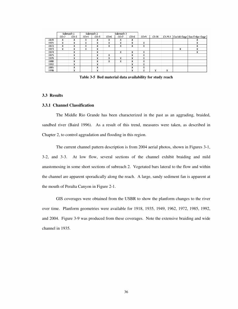
36
�Table 3-5 Bed material data availability for study reach
3.3 Results
3.3.1 Channel Classification
The Middle Rio Grande has been characterized in the past as an aggrading, braided,
sandbed river (Baird 1996). As a result of this trend, measures were taken, as described in
Chapter 2, to control aggradation and flooding in this region.
The current channel pattern description is from 2004 aerial photos, shown in Figures 3-1,
3-2, and 3-3. At low flow, several sections of the channel exhibit braiding and mild
anastomosing in some short sections of subreach 2. Vegetated bars lateral to the flow and within
the channel are apparent sporadically along the reach. A large, sandy sediment fan is apparent at
the mouth of Peralta Canyon in Figure 2-1.
GIS coverages were obtained from the USBR to show the planform changes to the river
over time. Planform geometries were available for 1918, 1935, 1949, 1962, 1972, 1985, 1992,
and 2004. Figure 3-9 was produced from these coverages. Note the extensive braiding and wide
channel in 1935.
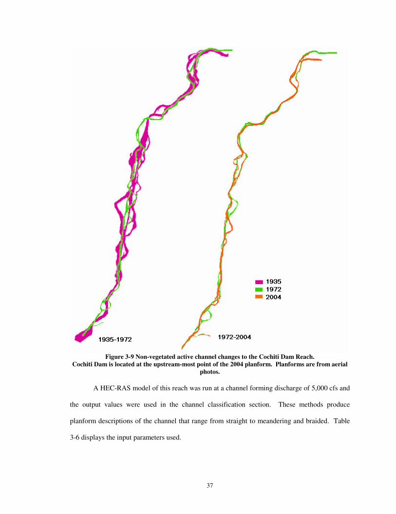
37
�Figure 3-9 Non-vegetated active channel changes to the Cochiti Dam Reach.
Cochiti Dam is located at the upstream-most point of the 2004 planform. Planforms are from aerial photos. �
A HEC-RAS model of this reach was run at a channel forming discharge of 5,000 cfs and
the output values were used in the channel classification section. These methods produce
planform descriptions of the channel that range from straight to meandering and braided. Table
3-6 displays the input parameters used.
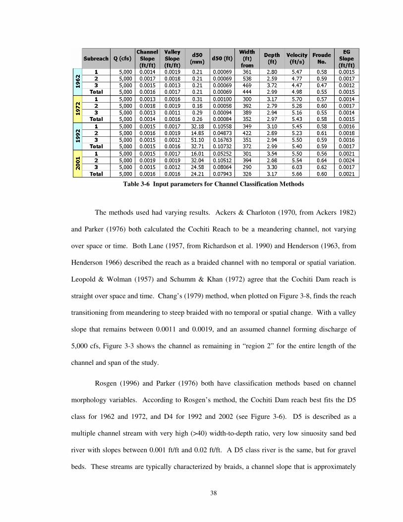
38
�Table 3-6 Input parameters for Channel Classification Methods
The methods used had varying results. Ackers & Charloton (1970, from Ackers 1982)
and Parker (1976) both calculated the Cochiti Reach to be a meandering channel, not varying
over space or time. Both Lane (1957, from Richardson et al. 1990) and Henderson (1963, from
Henderson 1966) described the reach as a braided channel with no temporal or spatial variation.
Leopold & Wolman (1957) and Schumm & Khan (1972) agree that the Cochiti Dam reach is
straight over space and time. Chang’s (1979) method, when plotted on Figure 3-8, finds the reach
transitioning from meandering to steep braided with no temporal or spatial change. With a valley
slope that remains between 0.0011 and 0.0019, and an assumed channel forming discharge of
5,000 cfs, Figure 3-3 shows the channel as remaining in “region 2” for the entire length of the
channel and span of the study.
Rosgen (1996) and Parker (1976) both have classification methods based on channel
morphology variables. According to Rosgen’s method, the Cochiti Dam reach best fits the D5
class for 1962 and 1972, and D4 for 1992 and 2002 (see Figure 3-6). D5 is described as a
multiple channel stream with very high (>40) width-to-depth ratio, very low sinuosity sand bed
river with slopes between 0.001 ft/ft and 0.02 ft/ft. A D5 class river is the same, but for gravel
beds. These streams are typically characterized by braids, a channel slope that is approximately

39
equivalent to the valley slope, and high bank erosion rates. Parker’s method describes the stream
to be meandering for all years, since the slope-to-Froude number ratio is much smaller than the
depth to width ratio.
Van de Berg’s (1995) method described the entire channel as a low sinuosity single
thread and multi thread channel in 1962 with no spatial variability. In 1972, the subreach
remained the same, with the exception of subreach 3, which is now classified as simply a single
thread channel. In 1992 and 2002, the entire length of the reach was reclassified as a single
thread channel. After the dam, the reach changed to a gravel bed river, and the potential specific
stream power for gravel bed rivers began to exceed the discriminator, as described in the methods
section.
Knighton and Nanson (1993) did not quantify threshold values for flow strength, bank
erodibility, and sediment supply. It is possible, however, to interpret the change in these
variables in the Cochiti Dam reach qualitatively. Just downstream of the dam, the discharge
peaks have decreased, and the sediment supply has been all but starved. Thus, the sediment
capacity has increased while the bank erodibility is high. Thus, the bed and banks of the
previously braided river have been eroded by the sediment starved clear water discharge from the
dam. This would suggest that the river has narrowed and deepened, transforming it from a
braided to a meandering planform.
The different channel classification methods employed varying parameters to estimate the
planform of the Cochiti Dam reach. Ackers and Charlton, Parker, Rosgen, and van den Berg
seemed to produce results that made physical sense (See Table 3-7).
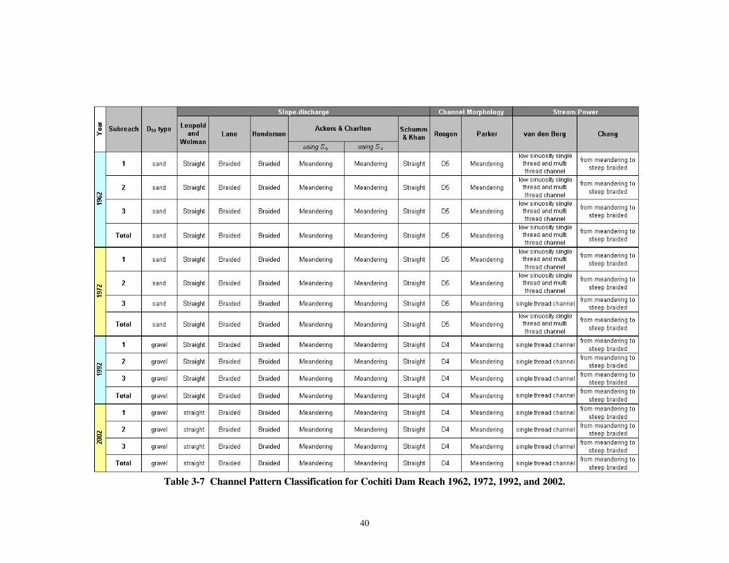
40
Table 3-7 Channel Pattern Classification for Cochiti Dam Reach 1962, 1972, 1992, and 2002.�
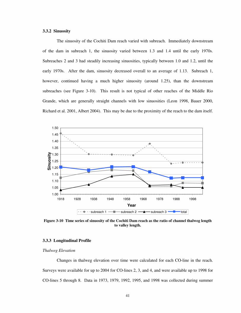
41
3.3.2 Sinuosity
The sinuosity of the Cochiti Dam reach varied with subreach. Immediately downstream
of the dam in subreach 1, the sinuosity varied between 1.3 and 1.4 until the early 1970s.
Subreaches 2 and 3 had steadily increasing sinuosities, typically between 1.0 and 1.2, until the
early 1970s. After the dam, sinuosity decreased overall to an average of 1.13. Subreach 1,
however, continued having a much higher sinuosity (around 1.25), than the downstream
subreaches (see Figure 3-10). This result is not typical of other reaches of the Middle Rio
Grande, which are generally straight channels with low sinuosities (Leon 1998, Bauer 2000,
Richard et al. 2001, Albert 2004). This may be due to the proximity of the reach to the dam itself.
1.00
1.05
1.10
1.15
1.20
1.25
1.30
1.35
1.40
1.45
1.50
1918 1928 1938 1948 1958 1968 1978 1988 1998
Year
Sin
uosi
ty
subreach 1 subreach 2 subreach 3 total
�Figure 3-10 Time series of sinuosity of the Cochiti Dam reach as the ratio of channel thalweg length
to valley length. � �
3.3.3 Longitudinal Profile
Thalweg Elevation
Changes in thalweg elevation over time were calculated for each CO-line in the reach.
Surveys were available for up to 2004 for CO-lines 2, 3, and 4, and were available up to 1998 for
CO-lines 5 through 8. Data in 1973, 1979, 1992, 1995, and 1998 was collected during summer
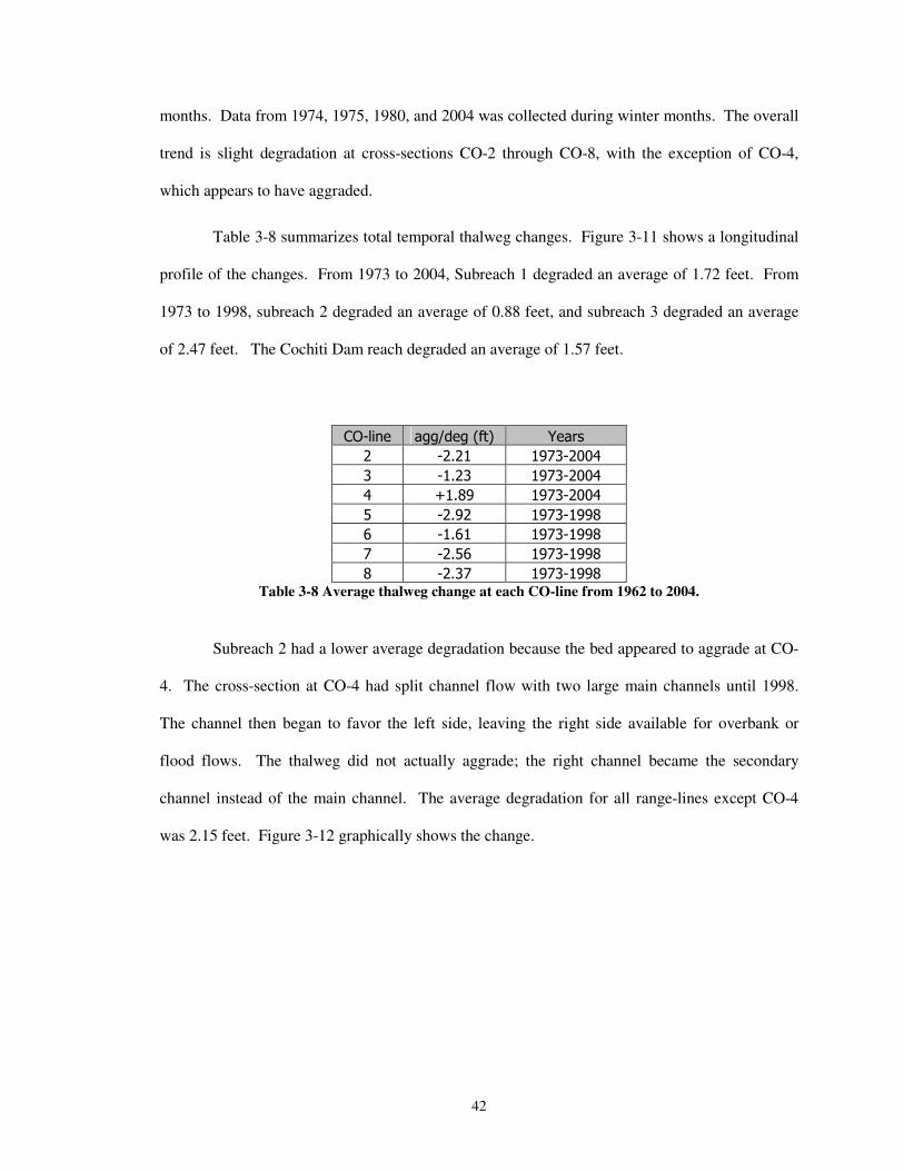
42
months. Data from 1974, 1975, 1980, and 2004 was collected during winter months. The overall
trend is slight degradation at cross-sections CO-2 through CO-8, with the exception of CO-4,
which appears to have aggraded.
Table 3-8 summarizes total temporal thalweg changes. Figure 3-11 shows a longitudinal
profile of the changes. From 1973 to 2004, Subreach 1 degraded an average of 1.72 feet. From
1973 to 1998, subreach 2 degraded an average of 0.88 feet, and subreach 3 degraded an average
of 2.47 feet. The Cochiti Dam reach degraded an average of 1.57 feet.
��
������� �..+/�.�0*�1� %��$&�
�� ��'�� �� ������
� �'� � �� ������
�� 2'��� �� ������
� ��'��� �� �����
�� �'�� �� �����
�� ��' �� �� �����
�� ��' �� �� �����Table 3-8 Average thalweg change at each CO-line from 1962 to 2004.
�
Subreach 2 had a lower average degradation because the bed appeared to aggrade at CO-
4. The cross-section at CO-4 had split channel flow with two large main channels until 1998.
The channel then began to favor the left side, leaving the right side available for overbank or
flood flows. The thalweg did not actually aggrade; the right channel became the secondary
channel instead of the main channel. The average degradation for all range-lines except CO-4
was 2.15 feet. Figure 3-12 graphically shows the change.
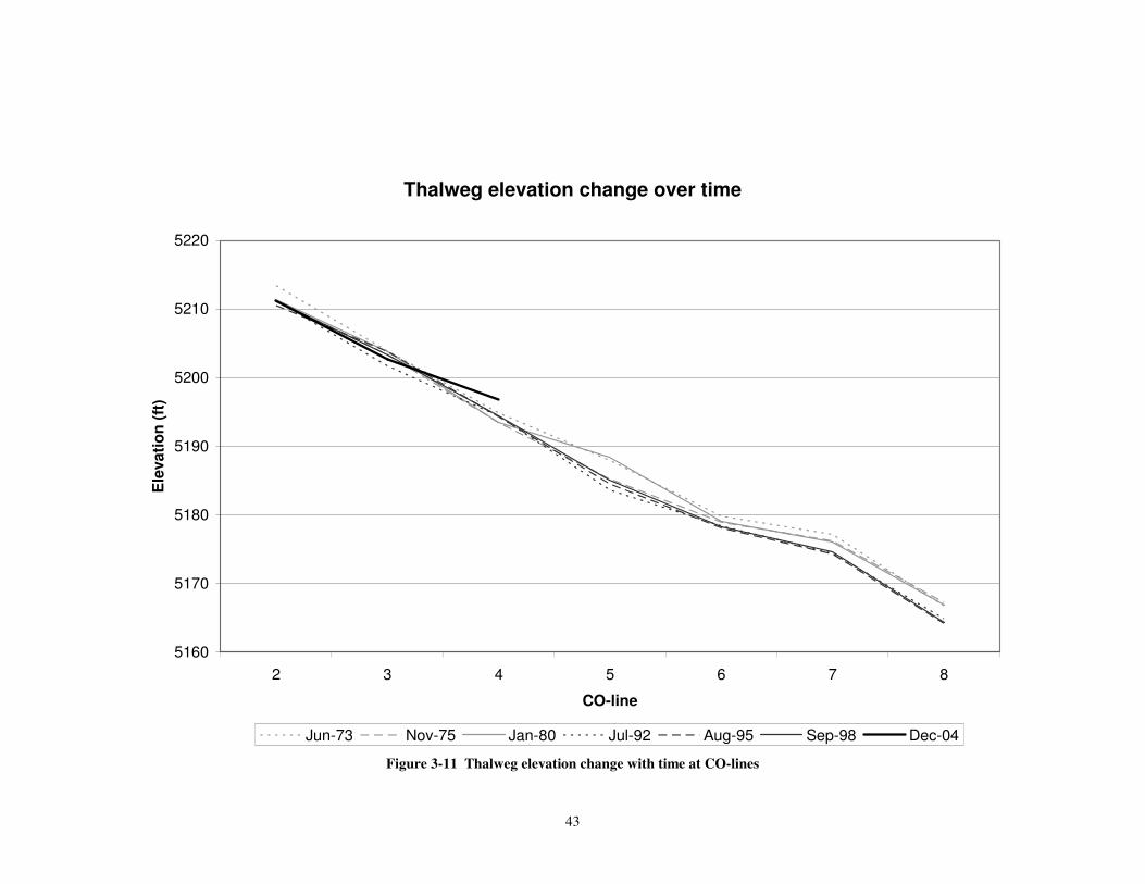
43
Thalweg elevation change over time
5160
5170
5180
5190
5200
5210
5220
2 3 4 5 6 7 8
CO-line
Ele
vatio
n (f
t)
Jun-73 Nov-75 Jan-80 Jul-92 Aug-95 Sep-98 Dec-04�
Figure 3-11 Thalweg elevation change with time at CO-lines
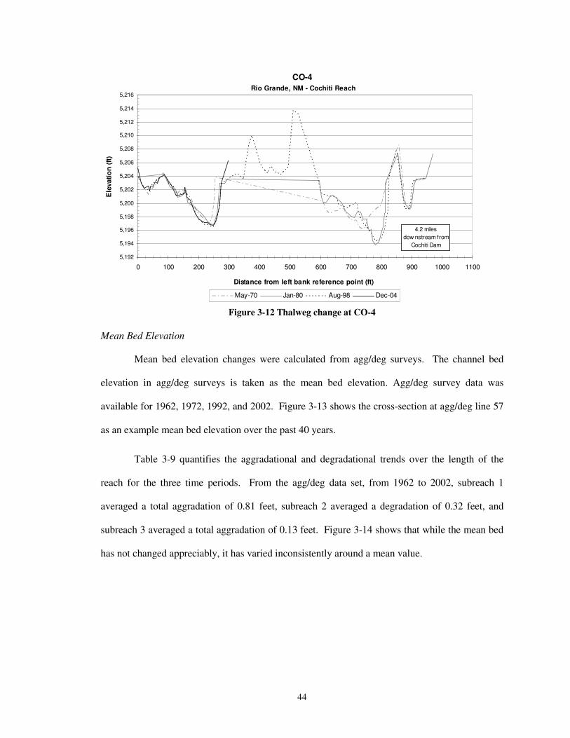
44
CO-4 Rio Grande, NM - Cochiti Reach
5,192
5,194
5,196
5,198
5,200
5,202
5,204
5,206
5,208
5,210
5,212
5,214
5,216
0 100 200 300 400 500 600 700 800 900 1000 1100
Distance from left bank reference point (ft)
Ele
vatio
n (ft
)
May-70 Jan-80 Aug-98 Dec-04
4.2 miles dow nstream from
Cochiti Dam
�Figure 3-12 Thalweg change at CO-4
�Mean Bed Elevation
Mean bed elevation changes were calculated from agg/deg surveys. The channel bed
elevation in agg/deg surveys is taken as the mean bed elevation. Agg/deg survey data was
available for 1962, 1972, 1992, and 2002. Figure 3-13 shows the cross-section at agg/deg line 57
as an example mean bed elevation over the past 40 years.
Table 3-9 quantifies the aggradational and degradational trends over the length of the
reach for the three time periods. From the agg/deg data set, from 1962 to 2002, subreach 1
averaged a total aggradation of 0.81 feet, subreach 2 averaged a degradation of 0.32 feet, and
subreach 3 averaged a total aggradation of 0.13 feet. Figure 3-14 shows that while the mean bed
has not changed appreciably, it has varied inconsistently around a mean value.
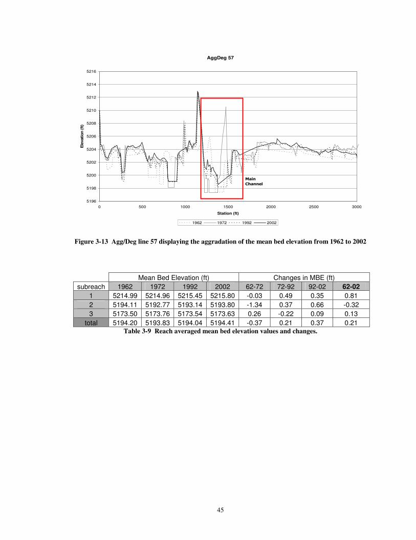
45
AggDeg 57
5196
5198
5200
5202
5204
5206
5208
5210
5212
5214
5216
0 500 1000 1500 2000 2500 3000
Station (ft)
Ele
vatio
n (f
t)
1962 1972 1992 2002
�����
�������
�
Figure 3-13 Agg/Deg line 57 displaying the aggradation of the mean bed elevation from 1962 to 2002 ���
Mean Bed Elevation (ft) Changes in MBE (ft) subreach 1962 1972 1992 2002 62-72 72-92 92-02 62-02
1 5214.99 5214.96 5215.45 5215.80 -0.03 0.49 0.35 0.81 2 5194.11 5192.77 5193.14 5193.80 -1.34 0.37 0.66 -0.32 3 5173.50 5173.76 5173.54 5173.63 0.26 -0.22 0.09 0.13
total 5194.20 5193.83 5194.04 5194.41 -0.37 0.21 0.37 0.21 Table 3-9 Reach averaged mean bed elevation values and changes.
�
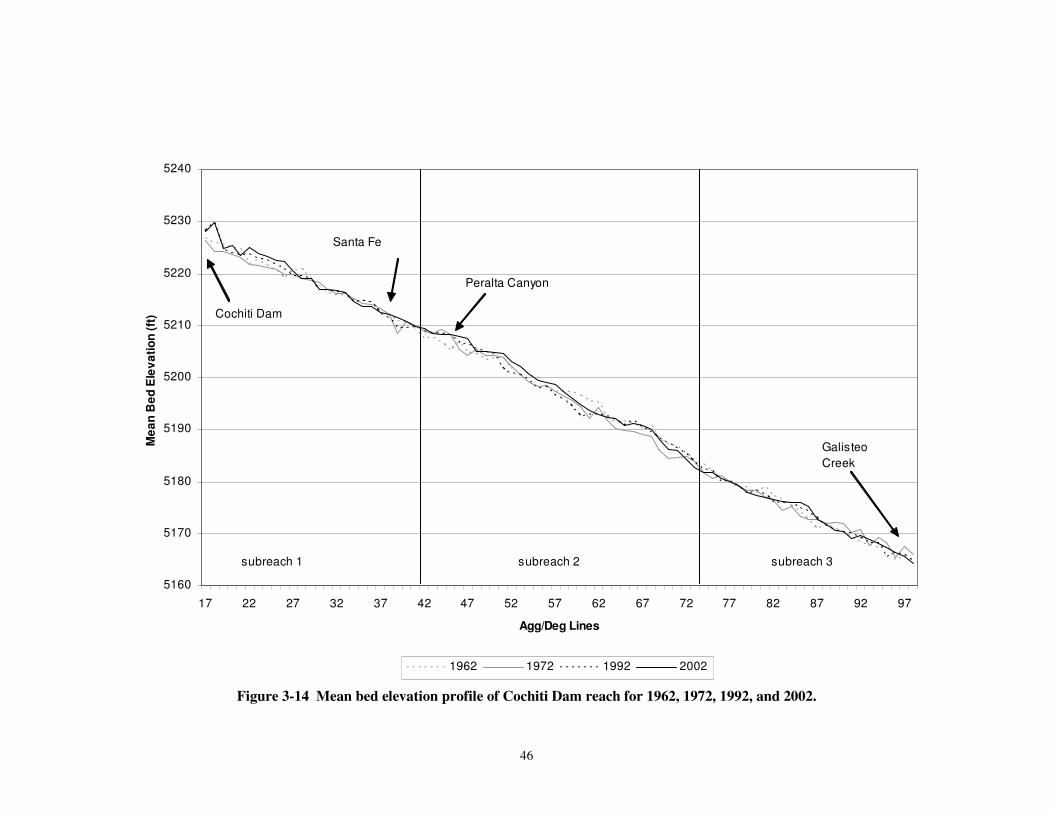
46
5160
5170
5180
5190
5200
5210
5220
5230
5240
17 22 27 32 37 42 47 52 57 62 67 72 77 82 87 92 97
Agg/Deg Lines
Mea
n B
ed E
leva
tion
(ft)
1962 1972 1992 2002
subreach 1 subreach 2 subreach 3
Cochiti Dam
Santa Fe
Galisteo Creek
Peralta Canyon
Figure 3-14 Mean bed elevation profile of Cochiti Dam reach for 1962, 1972, 1992, and 2002.
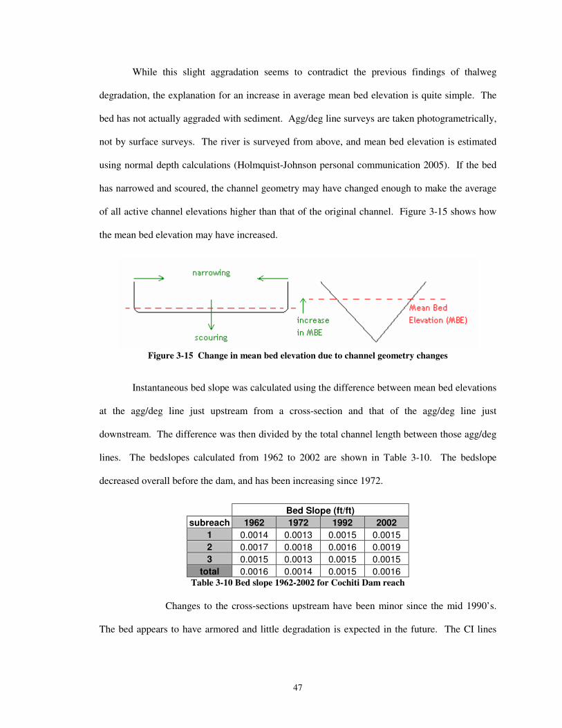
47
While this slight aggradation seems to contradict the previous findings of thalweg
degradation, the explanation for an increase in average mean bed elevation is quite simple. The
bed has not actually aggraded with sediment. Agg/deg line surveys are taken photogrametrically,
not by surface surveys. The river is surveyed from above, and mean bed elevation is estimated
using normal depth calculations (Holmquist-Johnson personal communication 2005). If the bed
has narrowed and scoured, the channel geometry may have changed enough to make the average
of all active channel elevations higher than that of the original channel. Figure 3-15 shows how
the mean bed elevation may have increased.
�Figure 3-15 Change in mean bed elevation due to channel geometry changes
Instantaneous bed slope was calculated using the difference between mean bed elevations
at the agg/deg line just upstream from a cross-section and that of the agg/deg line just
downstream. The difference was then divided by the total channel length between those agg/deg
lines. The bedslopes calculated from 1962 to 2002 are shown in Table 3-10. The bedslope
decreased overall before the dam, and has been increasing since 1972.
Bed Slope (ft/ft) subreach 1962 1972 1992 2002
1 0.0014 0.0013 0.0015 0.0015 2 0.0017 0.0018 0.0016 0.0019 3 0.0015 0.0013 0.0015 0.0015
total 0.0016 0.0014 0.0015 0.0016 Table 3-10 Bed slope 1962-2002 for Cochiti Dam reach
� Changes to the cross-sections upstream have been minor since the mid 1990’s.
The bed appears to have armored and little degradation is expected in the future. The CI lines
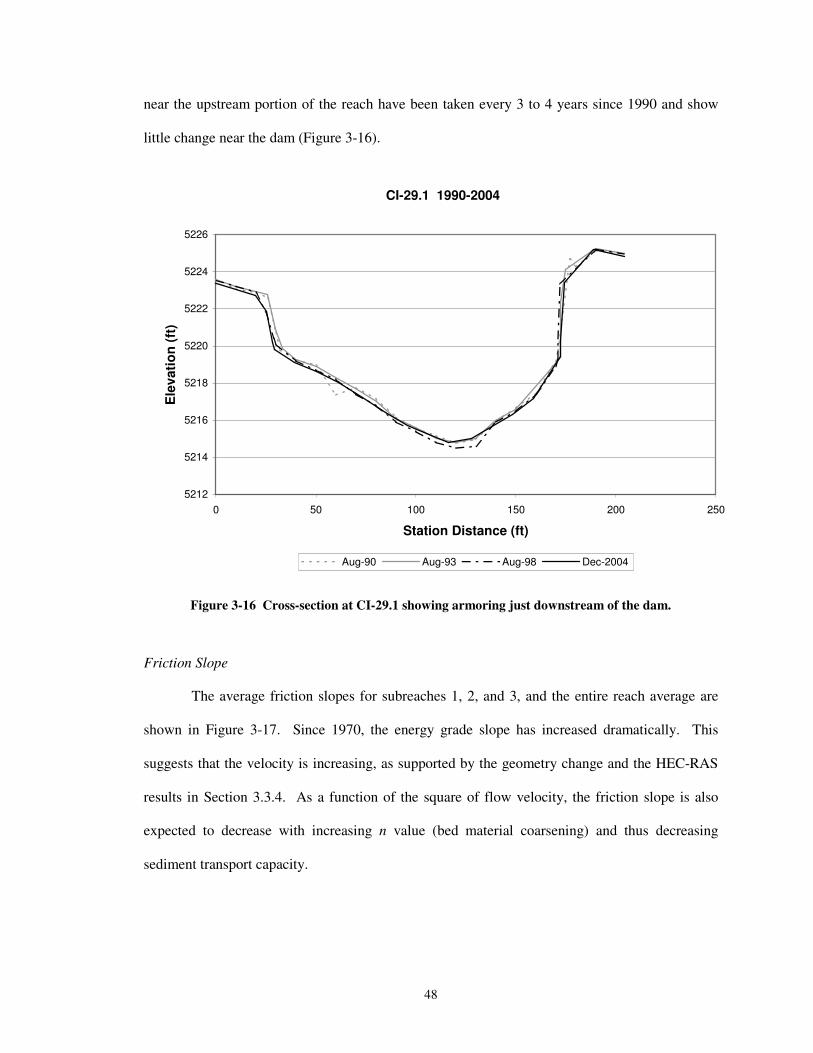
48
near the upstream portion of the reach have been taken every 3 to 4 years since 1990 and show
little change near the dam (Figure 3-16).
CI-29.1 1990-2004
5212
5214
5216
5218
5220
5222
5224
5226
0 50 100 150 200 250
Station Distance (ft)
Ele
vatio
n (f
t)
Aug-90 Aug-93 Aug-98 Dec-2004
�Figure 3-16 Cross-section at CI-29.1 showing armoring just downstream of the dam.
Friction Slope
The average friction slopes for subreaches 1, 2, and 3, and the entire reach average are
shown in Figure 3-17. Since 1970, the energy grade slope has increased dramatically. This
suggests that the velocity is increasing, as supported by the geometry change and the HEC-RAS
results in Section 3.3.4. As a function of the square of flow velocity, the friction slope is also
expected to decrease with increasing n value (bed material coarsening) and thus decreasing
sediment transport capacity.
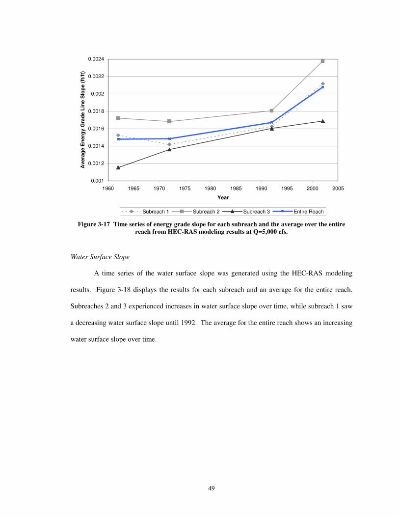
49
0.001
0.0012
0.0014
0.0016
0.0018
0.002
0.0022
0.0024
1960 1965 1970 1975 1980 1985 1990 1995 2000 2005
Year
Ave
rage
Ene
rgy
Gra
de L
ine
Slo
pe (f
t/ft)
Subreach 1 Subreach 2 Subreach 3 Entire Reach�
Figure 3-17 Time series of energy grade slope for each subreach and the average over the entire reach from HEC-RAS modeling results at Q=5,000 cfs.
��
Water Surface Slope
A time series of the water surface slope was generated using the HEC-RAS modeling
results. Figure 3-18 displays the results for each subreach and an average for the entire reach.
Subreaches 2 and 3 experienced increases in water surface slope over time, while subreach 1 saw
a decreasing water surface slope until 1992. The average for the entire reach shows an increasing
water surface slope over time.
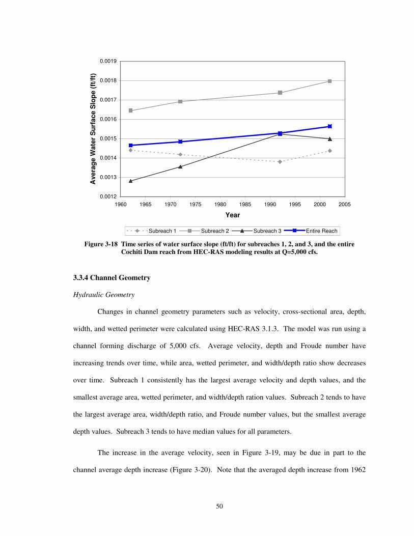
50
0.0012
0.0013
0.0014
0.0015
0.0016
0.0017
0.0018
0.0019
1960 1965 1970 1975 1980 1985 1990 1995 2000 2005
Year
Ave
rage
Wat
er S
urfa
ce S
lope
(ft/f
t)
Subreach 1 Subreach 2 Subreach 3 Entire Reach�
Figure 3-18 Time series of water surface slope (ft/ft) for subreaches 1, 2, and 3, and the entire Cochiti Dam reach from HEC-RAS modeling results at Q=5,000 cfs.
�
3.3.4 Channel Geometry
Hydraulic Geometry
Changes in channel geometry parameters such as velocity, cross-sectional area, depth,
width, and wetted perimeter were calculated using HEC-RAS 3.1.3. The model was run using a
channel forming discharge of 5,000 cfs. Average velocity, depth and Froude number have
increasing trends over time, while area, wetted perimeter, and width/depth ratio show decreases
over time. Subreach 1 consistently has the largest average velocity and depth values, and the
smallest average area, wetted perimeter, and width/depth ration values. Subreach 2 tends to have
the largest average area, width/depth ratio, and Froude number values, but the smallest average
depth values. Subreach 3 tends to have median values for all parameters.
The increase in the average velocity, seen in Figure 3-19, may be due in part to the
channel average depth increase (Figure 3-20). Note that the averaged depth increase from 1962
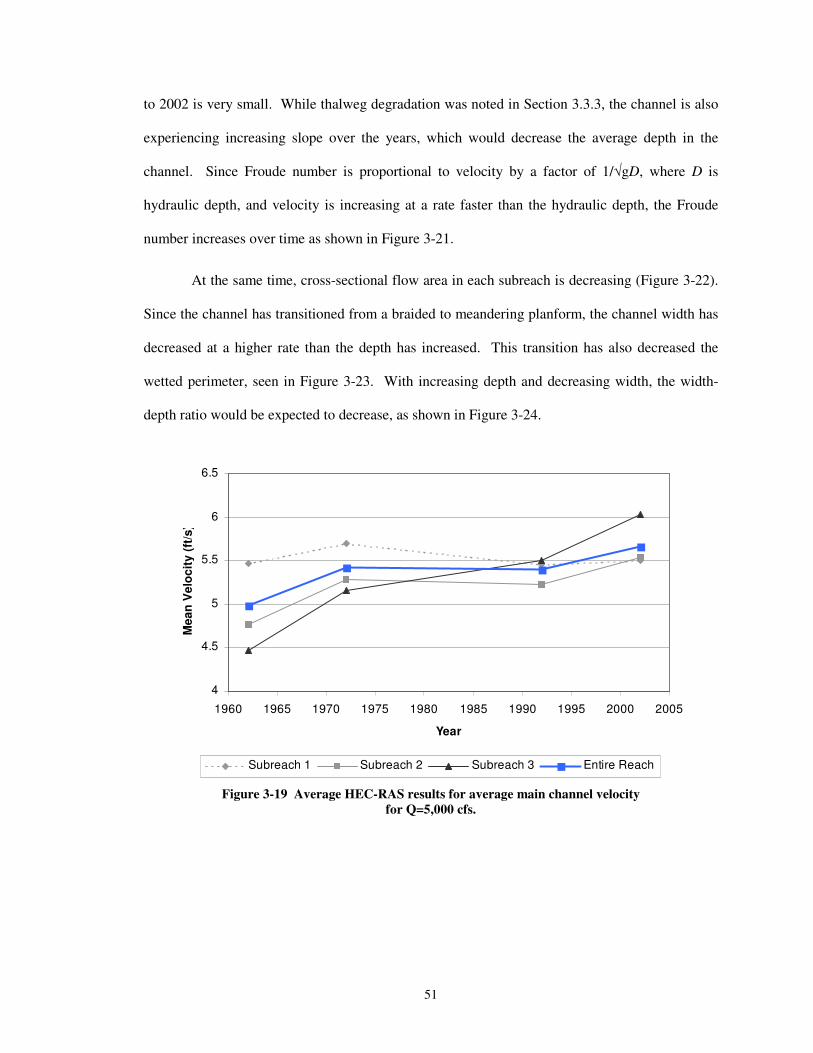
51
to 2002 is very small. While thalweg degradation was noted in Section 3.3.3, the channel is also
experiencing increasing slope over the years, which would decrease the average depth in the
channel. Since Froude number is proportional to velocity by a factor of 1/�gD, where D is
hydraulic depth, and velocity is increasing at a rate faster than the hydraulic depth, the Froude
number increases over time as shown in Figure 3-21. �
At the same time, cross-sectional flow area in each subreach is decreasing (Figure 3-22).
Since the channel has transitioned from a braided to meandering planform, the channel width has
decreased at a higher rate than the depth has increased. This transition has also decreased the
wetted perimeter, seen in Figure 3-23. With increasing depth and decreasing width, the width-
depth ratio would be expected to decrease, as shown in Figure 3-24.
4
4.5
5
5.5
6
6.5
1960 1965 1970 1975 1980 1985 1990 1995 2000 2005
Year
Mea
n V
eloc
ity (f
t/s)
Subreach 1 Subreach 2 Subreach 3 Entire Reach�
Figure 3-19 Average HEC-RAS results for average main channel velocity for Q=5,000 cfs.
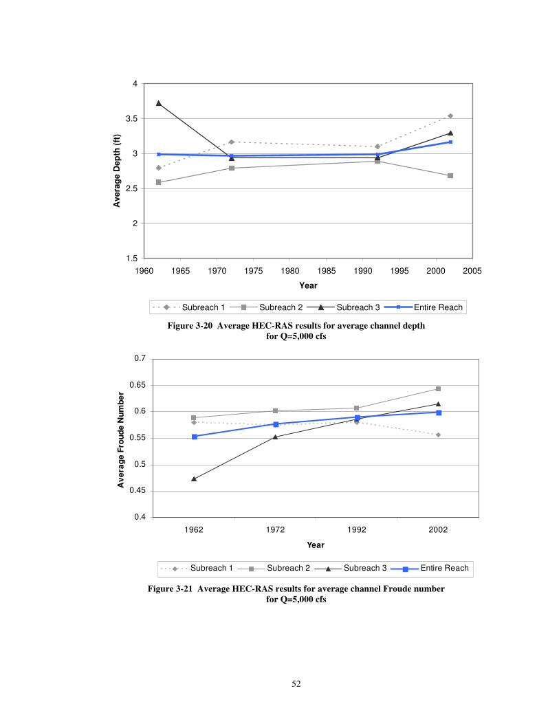
52
1.5
2
2.5
3
3.5
4
1960 1965 1970 1975 1980 1985 1990 1995 2000 2005
Year
Ave
rage
Dep
th (f
t)
Subreach 1 Subreach 2 Subreach 3 Entire Reach�
Figure 3-20 Average HEC-RAS results for average channel depth for Q=5,000 cfs
0.4
0.45
0.5
0.55
0.6
0.65
0.7
1962 1972 1992 2002
Year
Ave
rage
Fro
ude
Num
ber
Subreach 1 Subreach 2 Subreach 3 Entire Reach�
Figure 3-21 Average HEC-RAS results for average channel Froude number for Q=5,000 cfs
�
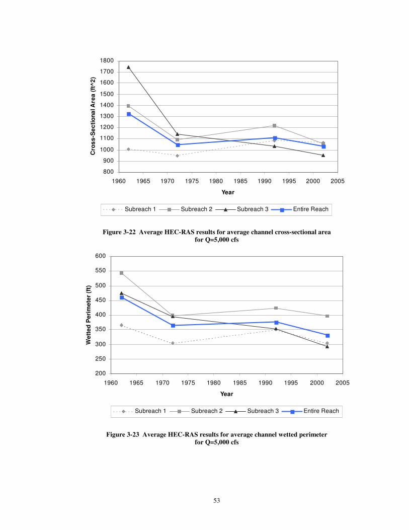
53
800
900
1000
1100
1200
1300
1400
1500
1600
1700
1800
1960 1965 1970 1975 1980 1985 1990 1995 2000 2005
Year
Cro
ss-S
ectio
nal A
rea
(ft^
2)
Subreach 1 Subreach 2 Subreach 3 Entire Reach�
Figure 3-22 Average HEC-RAS results for average channel cross-sectional area
for Q=5,000 cfs
200
250
300
350
400
450
500
550
600
1960 1965 1970 1975 1980 1985 1990 1995 2000 2005
Year
Wet
ted
Per
imet
er (f
t)
Subreach 1 Subreach 2 Subreach 3 Entire Reach�
�Figure 3-23 Average HEC-RAS results for average channel wetted perimeter
for Q=5,000 cfs
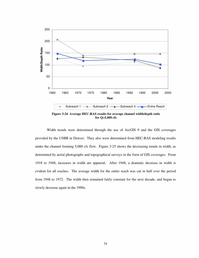
54
0
50
100
150
200
250
1960 1965 1970 1975 1980 1985 1990 1995 2000 2005
Year
Wid
th/D
epth
Rat
io
Subreach 1 Subreach 2 Subreach 3 Entire Reach�
Figure 3-24 Average HEC-RAS results for average channel width/depth ratio for Q=5,000 cfs
�
Width trends were determined through the use of ArcGIS 9 and the GIS coverages
provided by the USBR in Denver. They also were determined from HEC-RAS modeling results
under the channel forming 5,000 cfs flow. Figure 3-25 shows the decreasing trends in width, as
determined by aerial photographs and topographical surveys in the form of GIS coverages. From
1918 to 1948, increases in width are apparent. After 1948, a dramatic decrease in width is
evident for all reaches. The average width for the entire reach was cut in half over the period
from 1948 to 1972. The width then remained fairly constant for the next decade, and began to
slowly decrease again in the 1990s.
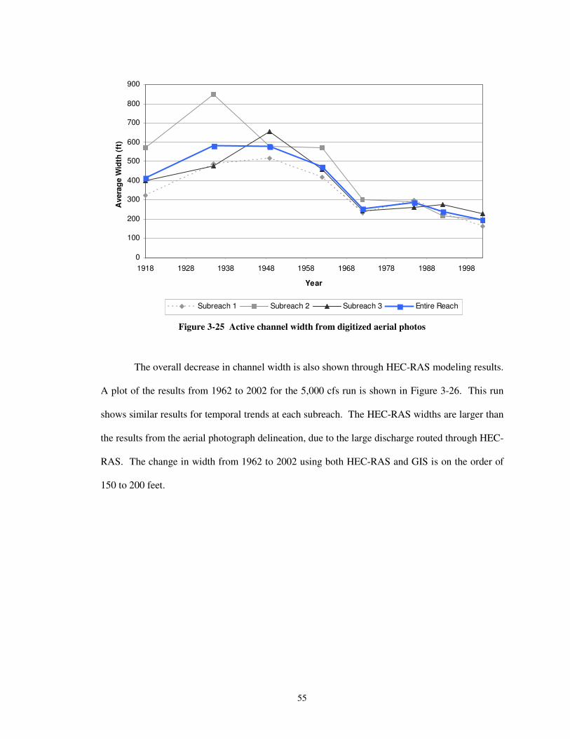
55
0
100
200
300
400
500
600
700
800
900
1918 1928 1938 1948 1958 1968 1978 1988 1998
Year
Ave
rage
Wid
th (f
t)
Subreach 1 Subreach 2 Subreach 3 Entire Reach
�Figure 3-25 Active channel width from digitized aerial photos
The overall decrease in channel width is also shown through HEC-RAS modeling results.
A plot of the results from 1962 to 2002 for the 5,000 cfs run is shown in Figure 3-26. This run
shows similar results for temporal trends at each subreach. The HEC-RAS widths are larger than
the results from the aerial photograph delineation, due to the large discharge routed through HEC-
RAS. The change in width from 1962 to 2002 using both HEC-RAS and GIS is on the order of
150 to 200 feet.
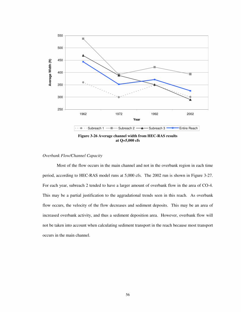
56
250
300
350
400
450
500
550
1962 1972 1992 2002
Year
Ave
rage
Wid
th (f
t)
Subreach 1 Subreach 2 Subreach 3 Entire Reach�
Figure 3-26 Average channel width from HEC-RAS results at Q=5,000 cfs
�
Overbank Flow/Channel Capacity
Most of the flow occurs in the main channel and not in the overbank region in each time
period, according to HEC-RAS model runs at 5,000 cfs. The 2002 run is shown in Figure 3-27.
For each year, subreach 2 tended to have a larger amount of overbank flow in the area of CO-4.
This may be a partial justification to the aggradational trends seen in this reach. As overbank
flow occurs, the velocity of the flow decreases and sediment deposits. This may be an area of
increased overbank activity, and thus a sediment deposition area. However, overbank flow will
not be taken into account when calculating sediment transport in the reach because most transport
occurs in the main channel.
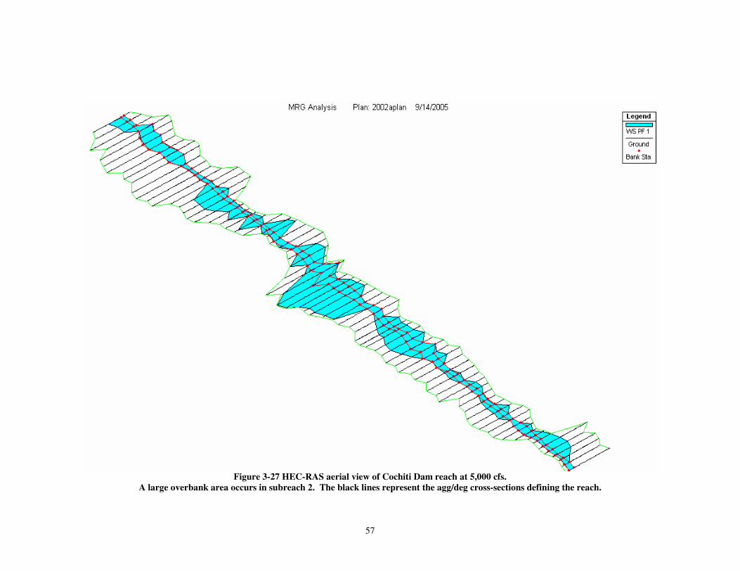
57
�Figure 3-27 HEC-RAS aerial view of Cochiti Dam reach at 5,000 cfs.
A large overbank area occurs in subreach 2. The black lines represent the agg/deg cross-sections defining the reach.
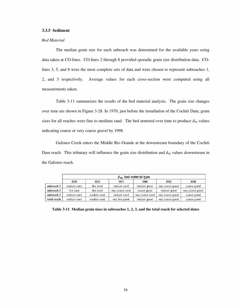
58
3.3.5 Sediment
Bed Material
The median grain size for each subreach was determined for the available years using
data taken at CO-lines. CO-lines 2 through 8 provided sporadic grain size distribution data. CO-
lines 3, 5, and 8 were the most complete sets of data and were chosen to represent subreaches 1,
2, and 3 respectively. Average values for each cross-section were computed using all
measurements taken.
Table 3-11 summarizes the results of the bed material analysis. The grain size changes
over time are shown in Figure 3-28. In 1970, just before the installation of the Cochiti Dam, grain
sizes for all reaches were fine to medium sand. The bed armored over time to produce d50 values
indicating coarse or very coarse gravel by 1998.
Galisteo Creek enters the Middle Rio Grande at the downstream boundary of the Cochiti
Dam reach. This tributary will influence the grain size distribution and d50 values downstream in
the Galisteo reach.
�
Table 3-11 Median grain sizes in subreaches 1, 2, 3, and the total reach for selected dates �
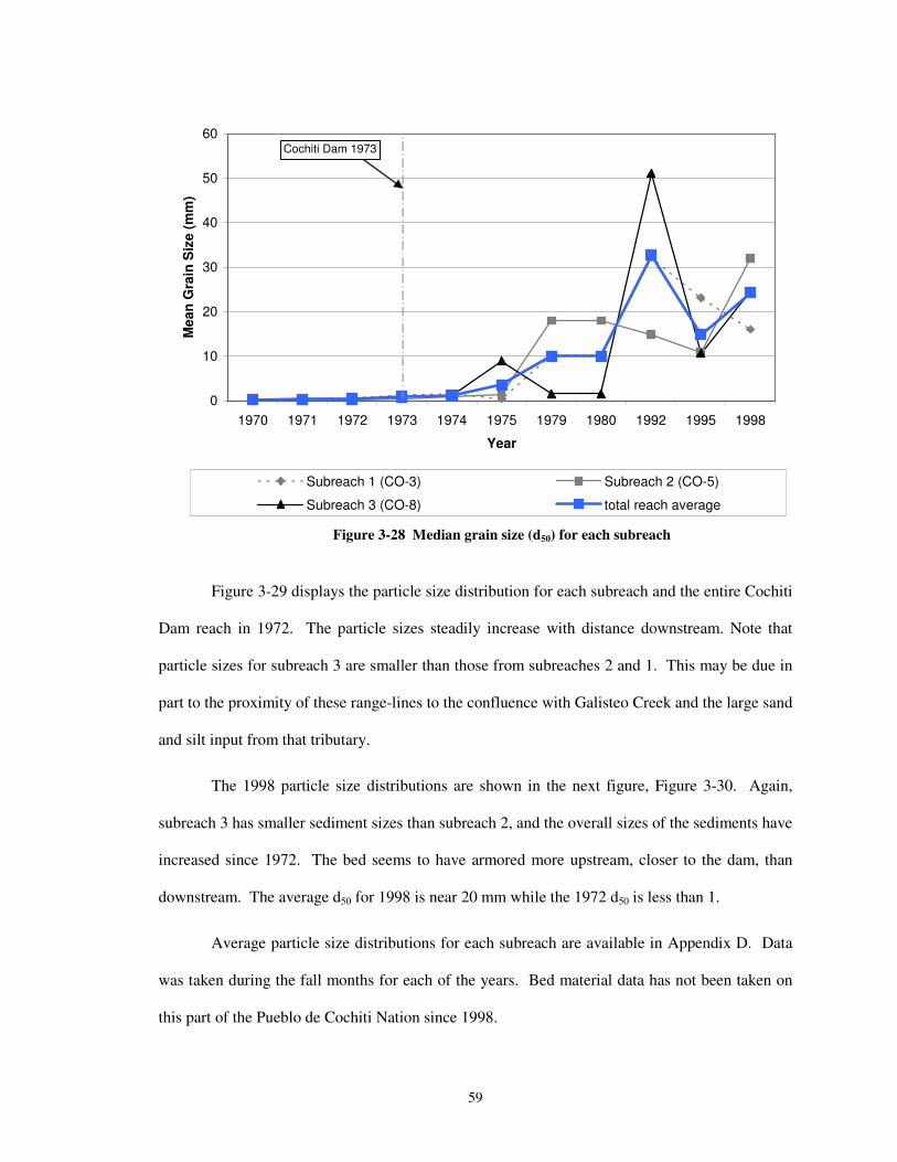
59
0
10
20
30
40
50
60
1970 1971 1972 1973 1974 1975 1979 1980 1992 1995 1998
Year
Mea
n G
rain
Siz
e (m
m)
Subreach 1 (CO-3) Subreach 2 (CO-5)
Subreach 3 (CO-8) total reach average
Cochiti Dam 1973
� Figure 3-28 Median grain size (d50) for each subreach
��
Figure 3-29 displays the particle size distribution for each subreach and the entire Cochiti
Dam reach in 1972. The particle sizes steadily increase with distance downstream. Note that
particle sizes for subreach 3 are smaller than those from subreaches 2 and 1. This may be due in
part to the proximity of these range-lines to the confluence with Galisteo Creek and the large sand
and silt input from that tributary.
The 1998 particle size distributions are shown in the next figure, Figure 3-30. Again,
subreach 3 has smaller sediment sizes than subreach 2, and the overall sizes of the sediments have
increased since 1972. The bed seems to have armored more upstream, closer to the dam, than
downstream. The average d50 for 1998 is near 20 mm while the 1972 d50 is less than 1.
Average particle size distributions for each subreach are available in Appendix D. Data
was taken during the fall months for each of the years. Bed material data has not been taken on
this part of the Pueblo de Cochiti Nation since 1998.
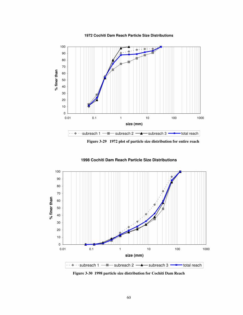
60
1972 Cochiti Dam Reach Particle Size Distributions
0
10
20
30
40
50
60
70
80
90
100
0.01 0.1 1 10 100 1000
size (mm)
% fi
ner
than
subreach 1 subreach 2 subreach 3 total reach�
Figure 3-29 1972 plot of particle size distribution for entire reach
1998 Cochiti Dam Reach Particle Size Distributions
0
10
20
30
40
50
60
70
80
90
100
0.01 0.1 1 10 100 1000
size (mm)
% fi
ner
than
subreach 1 subreach 2 subreach 3 total reach�
Figure 3-30 1998 particle size distribution for Cochiti Dam Reach
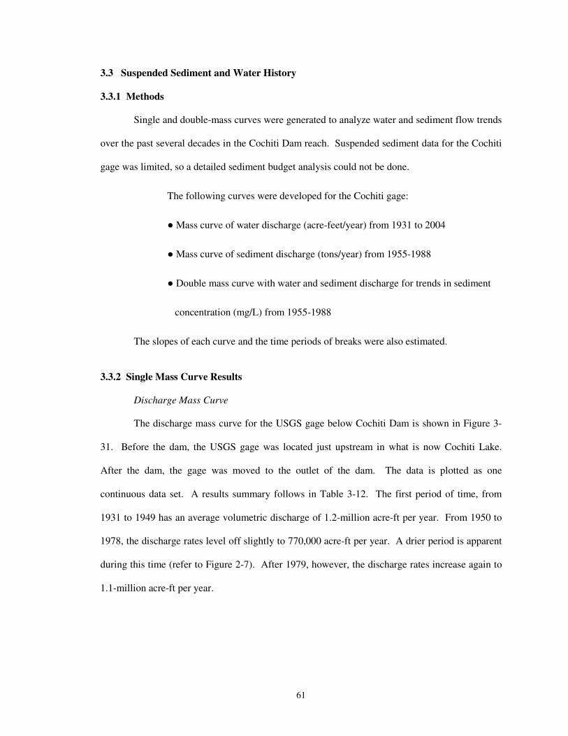
61
3.3 Suspended Sediment and Water History
3.3.1 Methods
Single and double-mass curves were generated to analyze water and sediment flow trends
over the past several decades in the Cochiti Dam reach. Suspended sediment data for the Cochiti
gage was limited, so a detailed sediment budget analysis could not be done.
The following curves were developed for the Cochiti gage:
� Mass curve of water discharge (acre-feet/year) from 1931 to 2004
� Mass curve of sediment discharge (tons/year) from 1955-1988
� Double mass curve with water and sediment discharge for trends in sediment
concentration (mg/L) from 1955-1988
The slopes of each curve and the time periods of breaks were also estimated.
3.3.2 Single Mass Curve Results
Discharge Mass Curve
The discharge mass curve for the USGS gage below Cochiti Dam is shown in Figure 3-
31. Before the dam, the USGS gage was located just upstream in what is now Cochiti Lake.
After the dam, the gage was moved to the outlet of the dam. The data is plotted as one
continuous data set. A results summary follows in Table 3-12. The first period of time, from
1931 to 1949 has an average volumetric discharge of 1.2-million acre-ft per year. From 1950 to
1978, the discharge rates level off slightly to 770,000 acre-ft per year. A drier period is apparent
during this time (refer to Figure 2-7). After 1979, however, the discharge rates increase again to
1.1-million acre-ft per year.
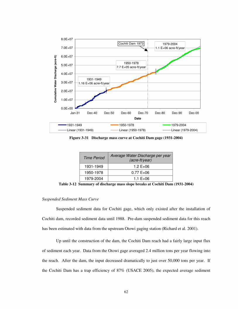
62
1931-19491.16 E+06 acre-ft/year
1950-19787.7 E+05 acre-ft/year
1979-20041.1 E+06 acre-ft/year
0.0E+00
1.0E+07
2.0E+07
3.0E+07
4.0E+07
5.0E+07
6.0E+07
7.0E+07
8.0E+07
Jan-31 Dec-40 Dec-50 Dec-60 Dec-70 Dec-80 Dec-90 Dec-00
Date
Cum
ulat
ive
Wat
er D
isch
arge
(acr
e-ft
)
1931-1949 1950-1978 1979-2004
Linear (1931-1949) Linear (1950-1978) Linear (1979-2004)
Cochiti Dam 1973
�Figure 3-31 Discharge mass curve at Cochiti Dam gage (1931-2004)
Time Period Average Water Discharge per year (acre-ft/year)
1931-1949 1.2 E+06
1950-1978 0.77 E+06
1979-2004 1.1 E+06 Table 3-12 Summary of discharge mass slope breaks at Cochiti Dam (1931-2004)
�
Suspended Sediment Mass Curve
Suspended sediment data for Cochiti gage, which only existed after the installation of
Cochiti dam, recorded sediment data until 1988. Pre-dam suspended sediment data for this reach
has been estimated with data from the upstream Otowi gaging station (Richard et al. 2001).
Up until the construction of the dam, the Cochiti Dam reach had a fairly large input flux
of sediment each year. Data from the Otowi gage averaged 2.4 million tons per year flowing into
the reach. After the dam, the input decreased dramatically to just over 50,000 tons per year. If
the Cochiti Dam has a trap efficiency of 87% (USACE 2005), the expected average sediment
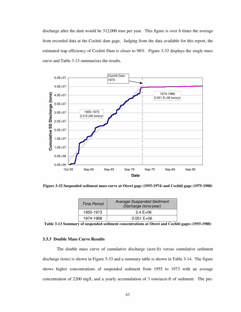
63
discharge after the dam would be 312,000 tons per year. This figure is over 6 times the average
from recorded data at the Cochiti dam gage. Judging from the data available for this report, the
estimated trap efficiency of Cochiti Dam is closer to 98%. Figure 3-32 displays the single mass
curve and Table 3-13 summarizes the results.
1955-19732.4 E+06 tons/yr
1974-19880.051 E+06 tons/yr
0.0E+00
5.0E+06
1.0E+07
1.5E+07
2.0E+07
2.5E+07
3.0E+07
3.5E+07
4.0E+07
4.5E+07
5.0E+07
Oct-55 Sep-60 Sep-65 Sep-70 Sep-75 Sep-80 Sep-85
Date
Cum
ulat
ive
SS
Dis
char
ge (t
ons)
Cochiti Dam 1973
�Figure 3-32 Suspended sediment mass curve at Otowi gage (1955-1974) and Cochiti gage (1975-1988)
��
Time Period Average Suspended Sediment Discharge (tons/year)
1955-1973 2.4 E+06
1974-1988 0.051 E+06 Table 3-13 Summary of suspended sediment concentrations at Otowi and Cochiti gages (1955-1988)
��
3.3.3 Double Mass Curve Results
The double mass curve of cumulative discharge (acre-ft) versus cumulative sediment
discharge (tons) is shown in Figure 3-33 and a summary table is shown in Table 3-14. The figure
shows higher concentrations of suspended sediment from 1955 to 1973 with an average
concentration of 2200 mg/L and a yearly accumulation of 3 tons/acre-ft of sediment. The pre-
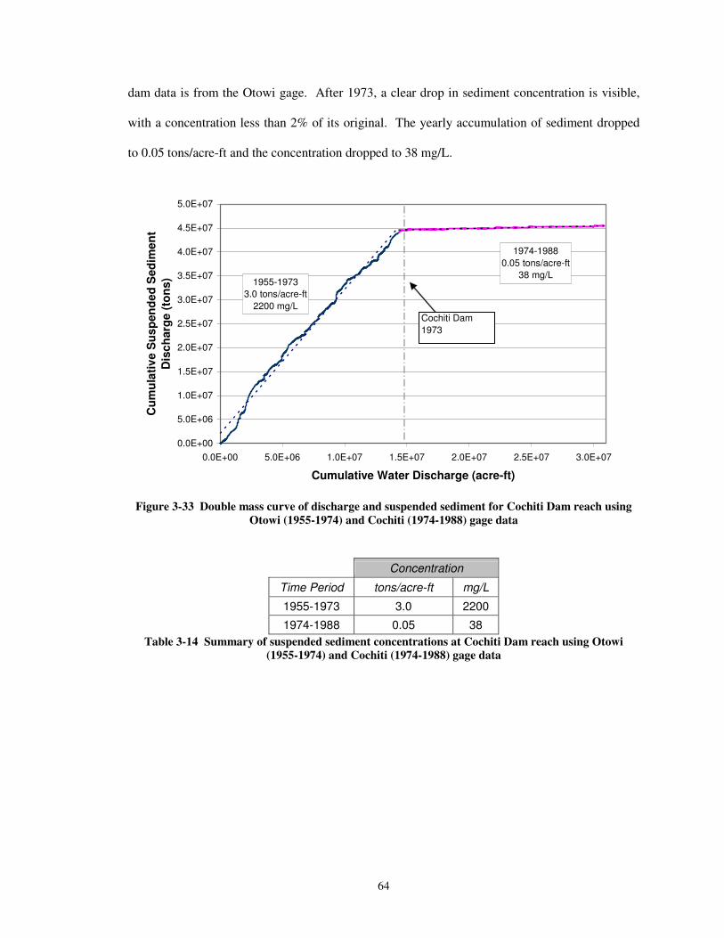
64
dam data is from the Otowi gage. After 1973, a clear drop in sediment concentration is visible,
with a concentration less than 2% of its original. The yearly accumulation of sediment dropped
to 0.05 tons/acre-ft and the concentration dropped to 38 mg/L.
1955-19733.0 tons/acre-ft
2200 mg/L
1974-19880.05 tons/acre-ft
38 mg/L
0.0E+00
5.0E+06
1.0E+07
1.5E+07
2.0E+07
2.5E+07
3.0E+07
3.5E+07
4.0E+07
4.5E+07
5.0E+07
0.0E+00 5.0E+06 1.0E+07 1.5E+07 2.0E+07 2.5E+07 3.0E+07
Cumulative Water Discharge (acre-ft)
Cum
ulat
ive
Sus
pend
ed S
edim
ent
Dis
char
ge (t
ons)
Cochiti Dam 1973
�Figure 3-33 Double mass curve of discharge and suspended sediment for Cochiti Dam reach using
Otowi (1955-1974) and Cochiti (1974-1988) gage data �
Concentration
Time Period tons/acre-ft mg/L
1955-1973 3.0 2200
1974-1988 0.05 38 Table 3-14 Summary of suspended sediment concentrations at Cochiti Dam reach using Otowi
(1955-1974) and Cochiti (1974-1988) gage data
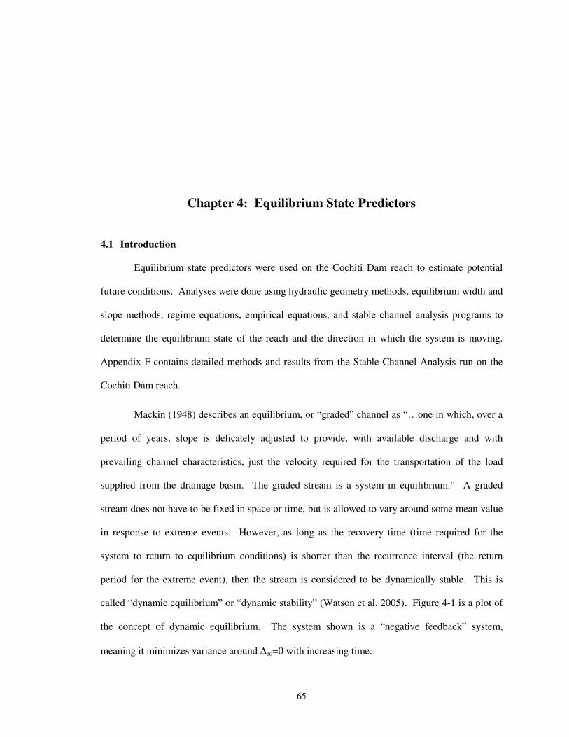
65
Chapter 4: Equilibrium State Predictors
4.1 Introduction
Equilibrium state predictors were used on the Cochiti Dam reach to estimate potential
future conditions. Analyses were done using hydraulic geometry methods, equilibrium width and
slope methods, regime equations, empirical equations, and stable channel analysis programs to
determine the equilibrium state of the reach and the direction in which the system is moving.
Appendix F contains detailed methods and results from the Stable Channel Analysis run on the
Cochiti Dam reach.
Mackin (1948) describes an equilibrium, or “graded” channel as “…one in which, over a
period of years, slope is delicately adjusted to provide, with available discharge and with
prevailing channel characteristics, just the velocity required for the transportation of the load
supplied from the drainage basin. The graded stream is a system in equilibrium.” A graded
stream does not have to be fixed in space or time, but is allowed to vary around some mean value
in response to extreme events. However, as long as the recovery time (time required for the
system to return to equilibrium conditions) is shorter than the recurrence interval (the return
period for the extreme event), then the stream is considered to be dynamically stable. This is
called “dynamic equilibrium” or “dynamic stability” (Watson et al. 2005). Figure 4-1 is a plot of
the concept of dynamic equilibrium. The system shown is a “negative feedback” system,
meaning it minimizes variance around ∆eq=0 with increasing time.
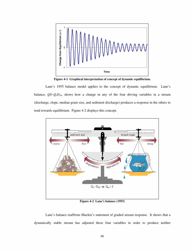
66
-1
0
1
Time
Cha
nge
from
Equ
ilibr
ium
(+/-)
�Figure 4-1 Graphical interpretation of concept of dynamic equilibrium.
Lane’s 1955 balance model applies to the concept of dynamic equilibrium. Lane’s
balance, QS~QsD50, shows how a change in any of the four driving variables in a stream
(discharge, slope, median grain size, and sediment discharge) produces a response in the others to
tend towards equilibrium. Figure 4-2 displays this concept.
�Figure 4-2 Lane’s balance (1955)
Lane’s balance reaffirms Mackin’s statement of graded stream response. It shows that a
dynamically stable stream has adjusted these four variables in order to produce neither
67
aggradation nor degradation in the stream, effectively transporting all available sediment through
the reach. In actuality, the situation of dynamic stability, when sediment input exactly matches
output, is a special case that won’t persist over long periods of time and that may only occur in
subreaches of a system (Watson et al. 2005).
Thus, in the Middle Rio Grande, major events such as floods, droughts, construction, or
other temporary variations may affect the channel regime. These local instabilities are the
stream’s response to the varying hydrologic inputs. This chapter will assess whether or not
equilibrium conditions can potentially exist, and if so, it will attempt to quantify these conditions.
4.2 Methods
4.2.1 Sediment Transport Analysis
The sediment load exiting Cochiti Dam is quite small (refer to Figure 3-31). After 1973,
the suspended sediment discharge out of the dam was only 0.05 tons/acre-ft (38 mg/L), or
approximately 2% of the suspended sediment discharging at the Otowi gage. This amount was
also approximately 9% of the sediment discharge occurring at the same time period at the
Bernalillo gage. The sediment discharge from Cochiti Dam may be assumed to be entirely
washload, due to the large settling basin upstream (Cochiti Reservoir) and the concrete footing at
the base of the dam, which prevents initial bedload transport. Since the sediment estimated from
Figure 3-33 is very small, the sediment discharge entering the reach is assumed to average 38
mg/L of washload. The equilibrium slope was calculated using the program developed by
Claudia Leon (2003) which estimates equilibrium slope for a reach with varying widths. This
will be discussed in the Equilbrium Channel Slope Analysis section.
Channel transport capacities for each subreach in the Cochiti Reach were estimated for
1962, 1972, 1992, and 2002 using the stable channel design tool in HEC-RAS 3.1.3. This
program utilized several different sediment transport equations: Laursen (1958), Engelund and
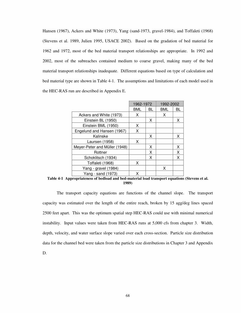
68
Hansen (1967), Ackers and White (1973), Yang (sand-1973, gravel-1984), and Toffaleti (1968)
(Stevens et al. 1989, Julien 1995, USACE 2002). Based on the gradation of bed material for
1962 and 1972, most of the bed material transport relationships are appropriate. In 1992 and
2002, most of the subreaches contained medium to coarse gravel, making many of the bed
material transport relationships inadequate. Different equations based on type of calculation and
bed material type are shown in Table 4-1. The assumptions and limitations of each model used in
the HEC-RAS run are described in Appendix E.
1962-1972 1992-2002 BML BL BML BL
Ackers and White (1973) X X Einstein BL (1950) X X
Einstein BML (1950) X Engelund and Hansen (1967) X
Kalinske X X Laursen (1958) X
Meyer-Peter and Müller (1948) X X Rottner X X
Schoklitsch (1934) X X Toffaleti (1968) X
Yang - gravel (1984) X Yang - sand (1973) X
Table 4-1 Appropriateness of bedload and bed-material load transport equations (Stevens et al. 1989) �
The transport capacity equations are functions of the channel slope. The transport
capacity was estimated over the length of the entire reach, broken by 15 agg/deg lines spaced
2500 feet apart. This was the optimum spatial step HEC-RAS could use with minimal numerical
instability. Input values were taken from HEC-RAS runs at 5,000 cfs from chapter 3. Width,
depth, velocity, and water surface slope varied over each cross-section. Particle size distribution
data for the channel bed were taken from the particle size distributions in Chapter 3 and Appendix
D.
69
4.2.2 Equilibrium Channel Slope Analysis
The equilibrium slope of the channel was estimated using the program created by Claudia
Leon (2003) for the Bosque del Apache reach of the Middle Rio Grande. This program utilizes
discharge, temperature, mean bed elevation, width, and sediment data to estimate the equilibrium
slope, time to equilibrium, aggradation, and degradation of the channel bed under certain
specified conditions. The program assumes that the width of the channel remains fixed over time,
although it may vary spatially.
The program was run using mean bed elevation, bed slope and width data from the three
subreaches from 1972, daily discharge and temperature data from the USGS from 1970 to 2004,
and median grain sizes from 1972.
In addition, depth to armoring was calculated to provide a base elevation in the reach to
which scouring was possible for each of the three subreaches. This was calculated by estimating
the minimum grain size at the beginning of motion, dsc, in each subreach. The scour depth, �z,
was then calculated based on the percent-finer value of each size claste at each subreach in each
year. Next, a maximum peak flow scouring was calculated. This result was added to the scour
calculated from 1972 to 1998 to estimate the total depth to armoring that is possible in the reach.
Each subreach retained a maximum scour depth during the model run to prevent infinite
degradation.
4.2.3 Hydraulic Geometry
Hydraulic geometry equations were obtained from several different sources. These
equations were developed to estimate the characteristics of stable channels under channel forming
discharge. These methods may incorporate bed material size, channel slope, sediment
concentration, or a combination of these. The equations were developed for simplified situations,
such as man-made canals or single-thread channels. Unless specified differently, the variable Q
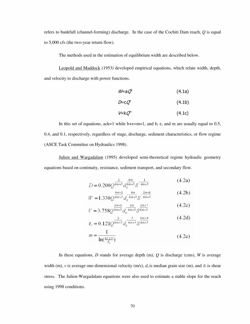
70
refers to bankfull (channel-forming) discharge. In the case of the Cochiti Dam reach, Q is equal
to 5,000 cfs (the two-year return flow).
The methods used in the estimation of equilibrium width are described below.
Leopold and Maddock (1953) developed empirical equations, which relate width, depth,
and velocity to discharge with power functions.
34�5��� � � 0�'�1�
�4�5�� � � � 0�'�1�
6475��� � � 0�'�1�
In this set of equations, ack=1 while b+e+m=1, and b, e, and m are usually equal to 0.5,
0.4, and 0.1, respectively, regardless of stage, discharge, sediment characteristics, or flow regime
(ASCE Task Committee on Hydraulics 1998).
Julien and Wargadalam (1995) developed semi-theoretical regime hydraulic geometry
equations based on continuity, resistance, sediment transport, and secondary flow.
In these equations, D stands for average depth (m), Q is discharge (cms), W is average
width (m), v is average one-dimensional velocity (m/s), ds is median grain size (m), and τ* is shear
stress. The Julien-Wargadalam equations were also used to estimate a stable slope for the reach
using 1998 conditions.
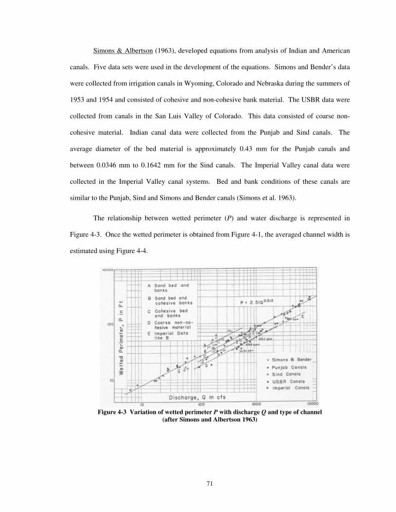
71
Simons & Albertson (1963), developed equations from analysis of Indian and American
canals. Five data sets were used in the development of the equations. Simons and Bender’s data
were collected from irrigation canals in Wyoming, Colorado and Nebraska during the summers of
1953 and 1954 and consisted of cohesive and non-cohesive bank material. The USBR data were
collected from canals in the San Luis Valley of Colorado. This data consisted of coarse non-
cohesive material. Indian canal data were collected from the Punjab and Sind canals. The
average diameter of the bed material is approximately 0.43 mm for the Punjab canals and
between 0.0346 mm to 0.1642 mm for the Sind canals. The Imperial Valley canal data were
collected in the Imperial Valley canal systems. Bed and bank conditions of these canals are
similar to the Punjab, Sind and Simons and Bender canals (Simons et al. 1963).
The relationship between wetted perimeter (P) and water discharge is represented in
Figure 4-3. Once the wetted perimeter is obtained from Figure 4-1, the averaged channel width is
estimated using Figure 4-4.
�Figure 4-3 Variation of wetted perimeter P with discharge Q and type of channel
(after Simons and Albertson 1963) �
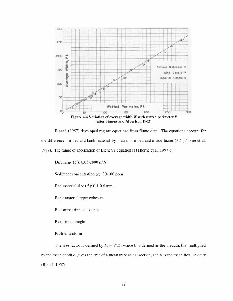
72
� Figure 4-4 Variation of average width W with wetted perimeter P
(after Simons and Albertson 1963) �
Blench (1957) developed regime equations from flume data. The equations account for
the differences in bed and bank material by means of a bed and a side factor (Fs) (Thorne et al.
1997). The range of application of Blench’s equation is (Thorne et al. 1997):
Discharge (Q): 0.03-2800 m3/s
Sediment concentration (c): 30-100 ppm
Bed material size (ds): 0.1-0.6 mm
Bank material type: cohesive
Bedforms: ripples – dunes
Planform: straight
Profile: uniform
The size factor is defined by Fs = V3/b, where b is defined as the breadth, that multiplied
by the mean depth d, gives the area of a mean trapezoidal section, and V is the mean flow velocity
(Blench 1957).
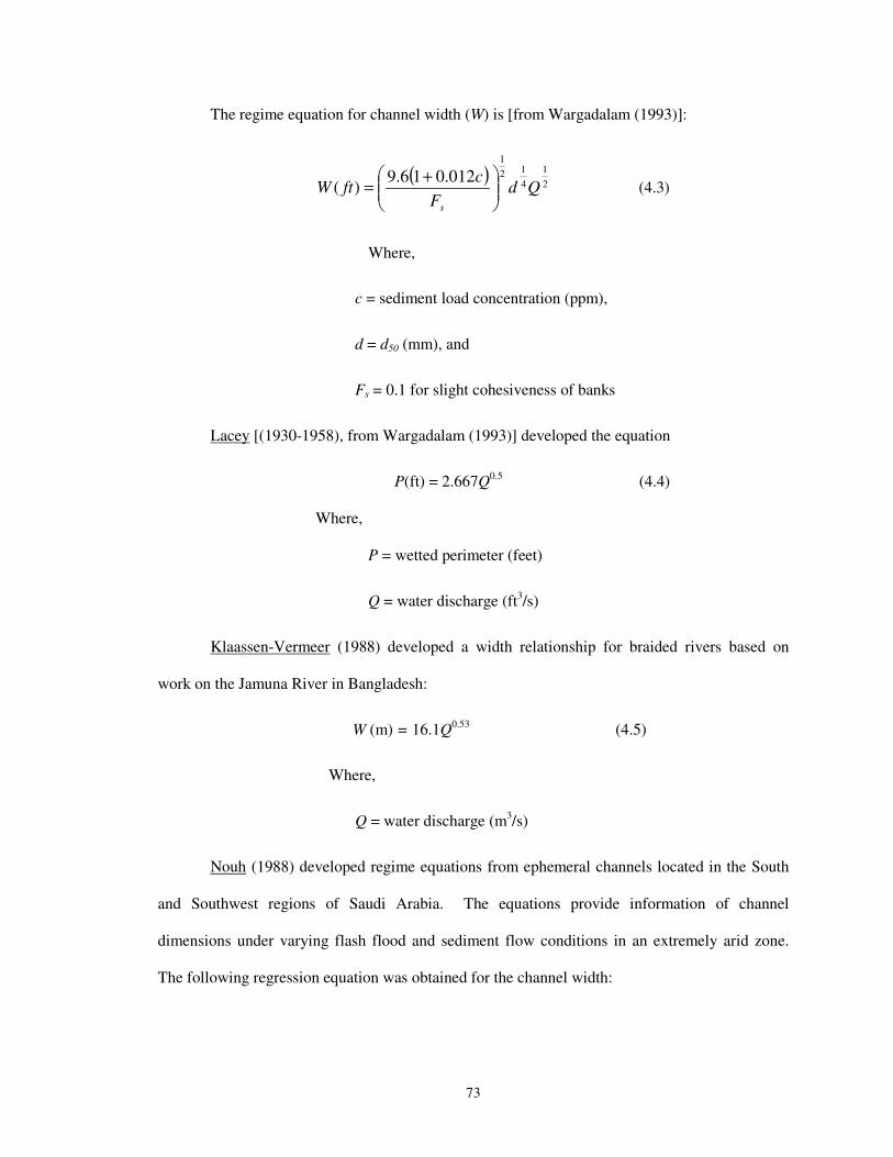
73
The regime equation for channel width (W) is [from Wargadalam (1993)]:
( ) 21
412
1
012.016.9)( Qd
Fc
ftWs
���
����
� += (4.3)
Where,
c = sediment load concentration (ppm),
d = d50 (mm), and
Fs = 0.1 for slight cohesiveness of banks
Lacey [(1930-1958), from Wargadalam (1993)] developed the equation
P(ft) = 2.667Q0.5 (4.4)
Where,
P = wetted perimeter (feet)
Q = water discharge (ft3/s)
Klaassen-Vermeer (1988) developed a width relationship for braided rivers based on
work on the Jamuna River in Bangladesh:
W (m) = 16.1Q0.53 (4.5)
Where,
Q = water discharge (m3/s)
Nouh (1988) developed regime equations from ephemeral channels located in the South
and Southwest regions of Saudi Arabia. The equations provide information of channel
dimensions under varying flash flood and sediment flow conditions in an extremely arid zone.
The following regression equation was obtained for the channel width:
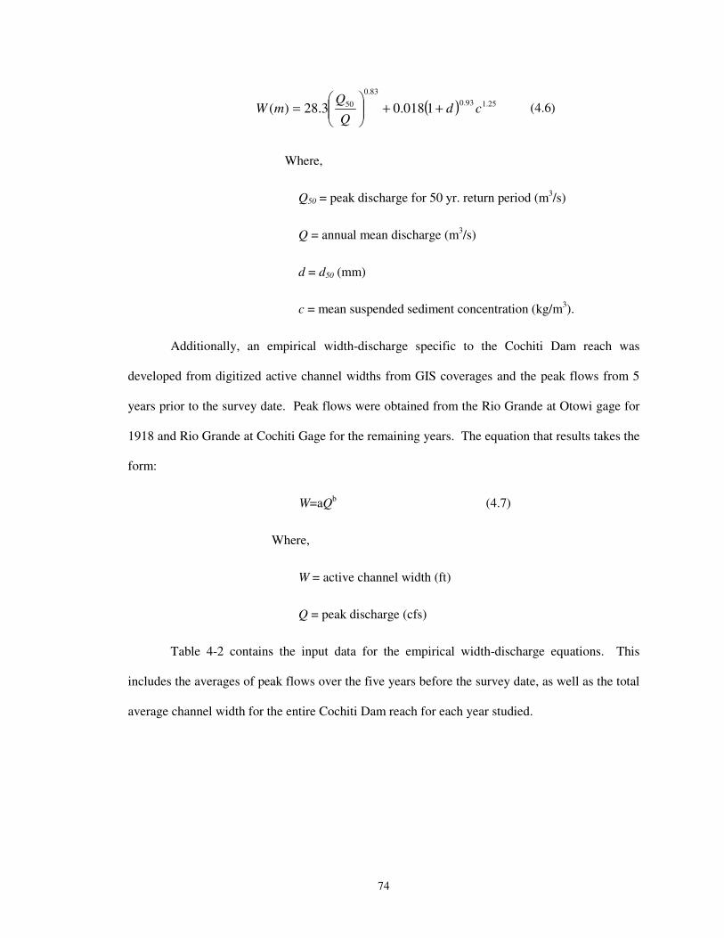
74
( ) 25.193.083.0
50 1018.03.28)( cdQ
QmW ++��
�
����
�= (4.6)
Where,
Q50 = peak discharge for 50 yr. return period (m3/s)
Q = annual mean discharge (m3/s)
d = d50 (mm)
c = mean suspended sediment concentration (kg/m3).
Additionally, an empirical width-discharge specific to the Cochiti Dam reach was
developed from digitized active channel widths from GIS coverages and the peak flows from 5
years prior to the survey date. Peak flows were obtained from the Rio Grande at Otowi gage for
1918 and Rio Grande at Cochiti Gage for the remaining years. The equation that results takes the
form:
W=aQb (4.7)
Where,
W = active channel width (ft)
Q = peak discharge (cfs)
Table 4-2 contains the input data for the empirical width-discharge equations. This
includes the averages of peak flows over the five years before the survey date, as well as the total
average channel width for the entire Cochiti Dam reach for each year studied.
�
�
�
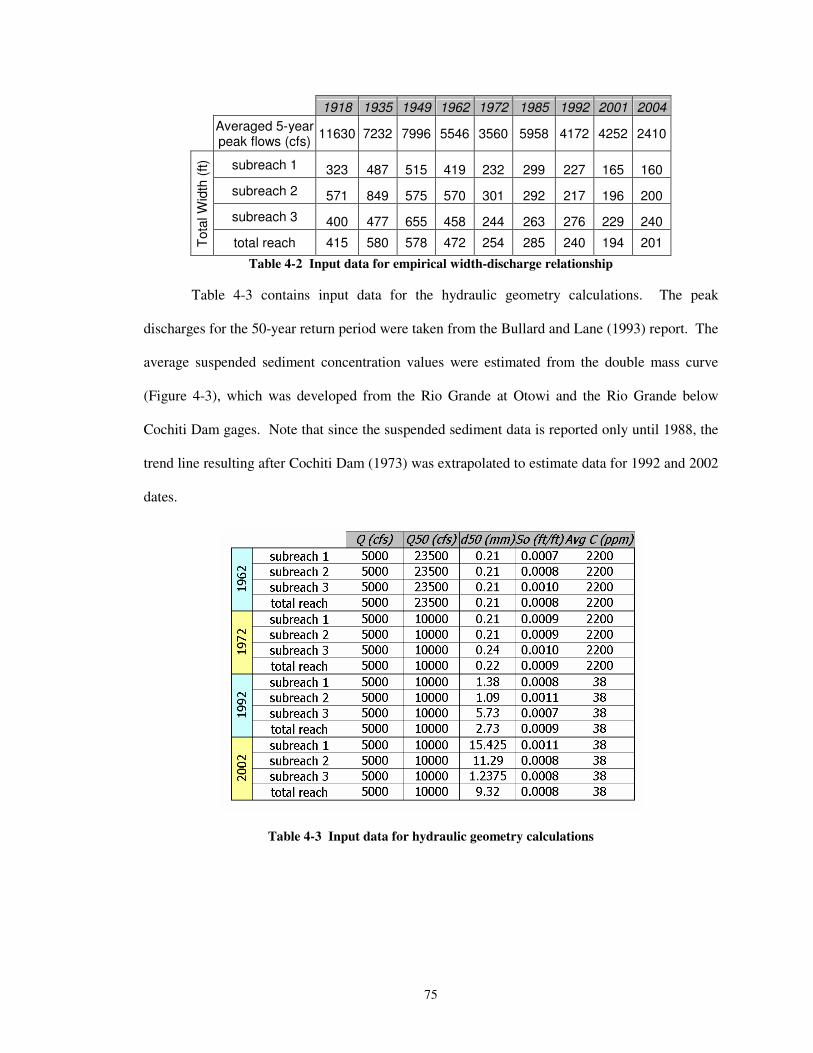
75
1918 1935 1949 1962 1972 1985 1992 2001 2004
Averaged 5-year peak flows (cfs) 11630 7232 7996 5546 3560 5958 4172 4252 2410
subreach 1 323 487 515 419 232 299 227 165 160
subreach 2 571 849 575 570 301 292 217 196 200
subreach 3 400 477 655 458 244 263 276 229 240 To
tal W
idth
(ft)
total reach 415 580 578 472 254 285 240 194 201
Table 4-2 Input data for empirical width-discharge relationship
Table 4-3 contains input data for the hydraulic geometry calculations. The peak
discharges for the 50-year return period were taken from the Bullard and Lane (1993) report. The
average suspended sediment concentration values were estimated from the double mass curve
(Figure 4-3), which was developed from the Rio Grande at Otowi and the Rio Grande below
Cochiti Dam gages. Note that since the suspended sediment data is reported only until 1988, the
trend line resulting after Cochiti Dam (1973) was extrapolated to estimate data for 1992 and 2002
dates.
�
Table 4-3 Input data for hydraulic geometry calculations
76
4.2.4 Equilibrium Channel Width
Williams and Wolman (1984) studied the downstream effects of dams on alluvial rivers.
The method developed describes the changes in channel width with time using hyperbolic
equations of the form:
(1/(Wt/Wi)) = C1 + C2 (1/t) (4.8)
Where,
Wt/Wi = the relative change in channel width,
C1 and C2 = empirical coefficients, and
t = time in years after the onset of the particular channel change.
The relative change in channel width is equal to the ratio of the width at time t (Wt) to the
initial width (Wi). Coefficients C1 and C2 may be functions of flow discharges and boundary
materials.
Hyperbolic equations were fitted to the entire Cochiti Dam reach and to each subreach
data set from 1949 to 2004. The time t = 0 was taken as 1949, when narrowing of the channel
began. The data to which the hyperbolic regressions were applied are in Table 4-4.
�
�
�
�
�
�
�
�
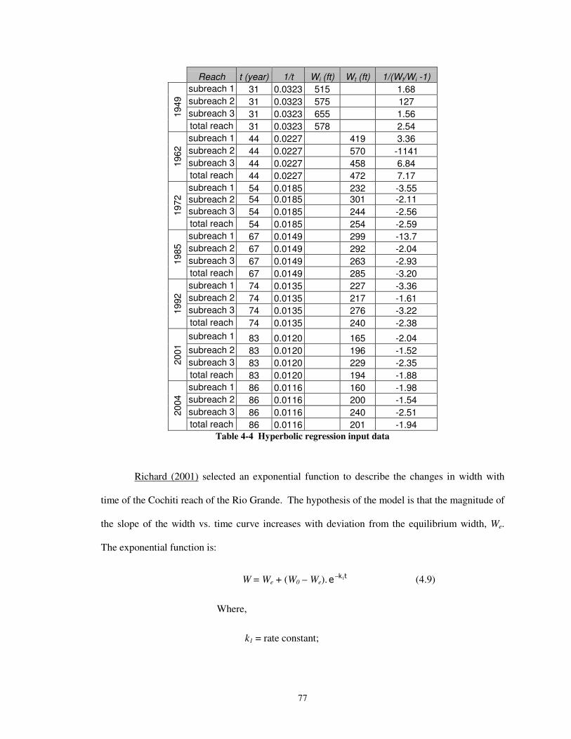
77
Reach t (year) 1/t Wi (ft) Wt (ft) 1/(Wt/Wi -1) subreach 1 31 0.0323 515 1.68 subreach 2 31 0.0323 575 127 subreach 3 31 0.0323 655 1.56 19
49
total reach 31 0.0323 578 2.54 subreach 1 44 0.0227 419 3.36 subreach 2 44 0.0227 570 -1141 subreach 3 44 0.0227 458 6.84 19
62
total reach 44 0.0227 472 7.17 subreach 1 54 0.0185 232 -3.55 subreach 2 54 0.0185 301 -2.11 subreach 3 54 0.0185 244 -2.56 19
72
total reach 54 0.0185 254 -2.59 subreach 1 67 0.0149 299 -13.7 subreach 2 67 0.0149 292 -2.04 subreach 3 67 0.0149 263 -2.93 19
85
total reach 67 0.0149 285 -3.20 subreach 1 74 0.0135 227 -3.36 subreach 2 74 0.0135 217 -1.61 subreach 3 74 0.0135 276 -3.22 19
92
total reach 74 0.0135 240 -2.38 subreach 1 83 0.0120 165 -2.04 subreach 2 83 0.0120 196 -1.52 subreach 3 83 0.0120 229 -2.35 20
01
total reach 83 0.0120 194 -1.88 subreach 1 86 0.0116 160 -1.98 subreach 2 86 0.0116 200 -1.54 subreach 3 86 0.0116 240 -2.51 20
04
total reach 86 0.0116 201 -1.94 Table 4-4 Hyperbolic regression input data
Richard (2001) selected an exponential function to describe the changes in width with
time of the Cochiti reach of the Rio Grande. The hypothesis of the model is that the magnitude of
the slope of the width vs. time curve increases with deviation from the equilibrium width, We.
The exponential function is:
W = We + (W0 – We). �7� 1− (4.9)
Where,
k1 = rate constant;
78
We = Equilibrium width toward which channel is moving (ft),
W0 = Channel width (ft) at time t0 (yrs), and
W = Channel width (ft) at time t (yrs).
Richard used three methods to estimate k1 and We. The first method consists of
empirically estimating the value of k1 and We by plotting the width change rate vs. the width and
generating a regression line. The rate constant, k1, is the slope of the regression line and the
intercept is k1We. The second method consists of using the empirically determined k-values from
the first method and varying the equilibrium width values to produce a “best-fit” equation that
minimized the sum-square error (SSE) between the predicted and observed widths. This method
was developed in an effort to better estimate the equilibrium width. The third method consists of
estimating the equilibrium width, We, using a hydraulic geometry equation. The k1-value was
determined by varying it until the SSE between the predicted and observed width was minimized.
In addition, a “Best Engineering Estimate” equation was estimated visually, as well as a
least-squares regression. These were plotted in addition to Richard’s method in an effort to
develop a better fit to the data. The least squares fit was developed by taking the partial
derivative of the exponential equation W=(a-c)e(-bt)+c with respect to each variable and setting
them equal to zero. This produced three equations and three variables which were solved
simultaneously.
�
4.3 Results
4.3.1 Sediment Transport Analysis
Sediment transport capacities were calculated for the Cochiti Dam reach using several
methods in HEC-RAS. Assuming all suspended sediment discharge consists of washload when
entering the reach, Figure 4-5 shows the sediment rating curve for suspended sediment
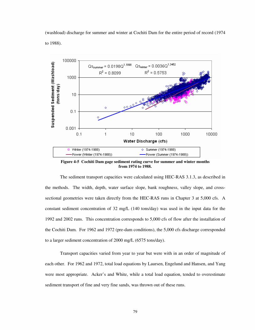
79
(washload) discharge for summer and winter at Cochiti Dam for the entire period of record (1974
to 1988).
�Figure 4-5 Cochiti Dam gage sediment rating curve for summer and winter months
from 1974 to 1988. �
The sediment transport capacities were calculated using HEC-RAS 3.1.3, as described in
the methods. The width, depth, water surface slope, bank roughness, valley slope, and cross-
sectional geometries were taken directly from the HEC-RAS runs in Chapter 3 at 5,000 cfs. A
constant sediment concentration of 32 mg/L (140 tons/day) was used in the input data for the
1992 and 2002 runs. This concentration corresponds to 5,000 cfs of flow after the installation of
the Cochiti Dam. For 1962 and 1972 (pre-dam conditions), the 5,000 cfs discharge corresponded
to a larger sediment concentration of 2000 mg/L (6575 tons/day).
Transport capacities varied from year to year but were with in an order of magnitude of
each other. For 1962 and 1972, total load equations by Laursen, Engelund and Hansen, and Yang
were most appropriate. Acker’s and White, while a total load equation, tended to overestimate
sediment transport of fine and very fine sands, was thrown out of these runs.
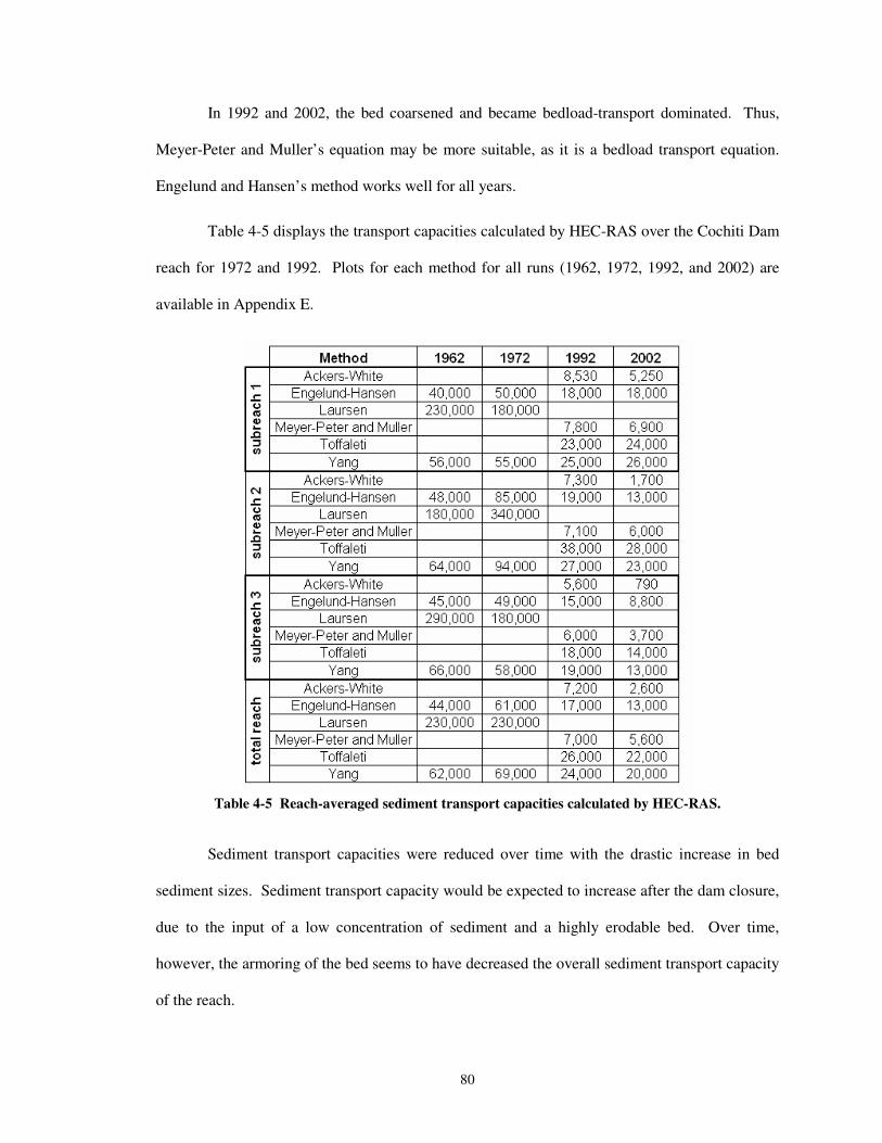
80
In 1992 and 2002, the bed coarsened and became bedload-transport dominated. Thus,
Meyer-Peter and Muller’s equation may be more suitable, as it is a bedload transport equation.
Engelund and Hansen’s method works well for all years.
Table 4-5 displays the transport capacities calculated by HEC-RAS over the Cochiti Dam
reach for 1972 and 1992. Plots for each method for all runs (1962, 1972, 1992, and 2002) are
available in Appendix E.
�Table 4-5 Reach-averaged sediment transport capacities calculated by HEC-RAS.
Sediment transport capacities were reduced over time with the drastic increase in bed
sediment sizes. Sediment transport capacity would be expected to increase after the dam closure,
due to the input of a low concentration of sediment and a highly erodable bed. Over time,
however, the armoring of the bed seems to have decreased the overall sediment transport capacity
of the reach.
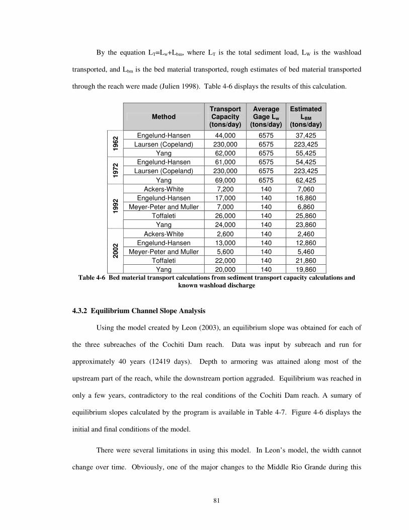
81
By the equation LT=Lw+Lbm, where LT is the total sediment load, LW is the washload
transported, and Lbm is the bed material transported, rough estimates of bed material transported
through the reach were made (Julien 1998). Table 4-6 displays the results of this calculation.
Method
Transport Capacity
(tons/day)
Average Gage Lw
(tons/day)
Estimated LBM
(tons/day)
Engelund-Hansen 44,000 6575 37,425 Laursen (Copeland) 230,000 6575 223,425
1962
Yang 62,000 6575 55,425 Engelund-Hansen 61,000 6575 54,425
Laursen (Copeland) 230,000 6575 223,425
1972
Yang 69,000 6575 62,425 Ackers-White 7,200 140 7,060
Engelund-Hansen 17,000 140 16,860 Meyer-Peter and Muller 7,000 140 6,860
Toffaleti 26,000 140 25,860
1992
Yang 24,000 140 23,860 Ackers-White 2,600 140 2,460
Engelund-Hansen 13,000 140 12,860 Meyer-Peter and Muller 5,600 140 5,460
Toffaleti 22,000 140 21,860
2002
Yang 20,000 140 19,860 Table 4-6 Bed material transport calculations from sediment transport capacity calculations and
known washload discharge �
4.3.2 Equilibrium Channel Slope Analysis
Using the model created by Leon (2003), an equilibrium slope was obtained for each of
the three subreaches of the Cochiti Dam reach. Data was input by subreach and run for
approximately 40 years (12419 days). Depth to armoring was attained along most of the
upstream part of the reach, while the downstream portion aggraded. Equilibrium was reached in
only a few years, contradictory to the real conditions of the Cochiti Dam reach. A sumary of
equilibrium slopes calculated by the program is available in Table 4-7. Figure 4-6 displays the
initial and final conditions of the model.
There were several limitations in using this model. In Leon’s model, the width cannot
change over time. Obviously, one of the major changes to the Middle Rio Grande during this
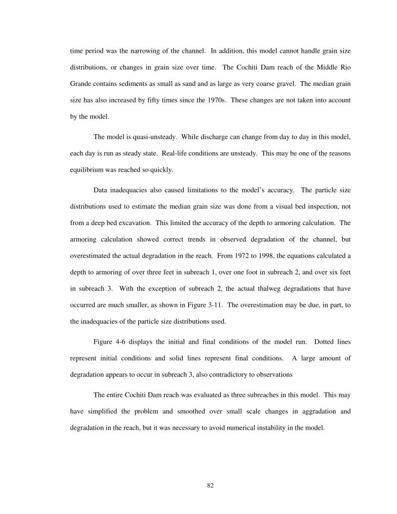
82
time period was the narrowing of the channel. In addition, this model cannot handle grain size
distributions, or changes in grain size over time. The Cochiti Dam reach of the Middle Rio
Grande contains sediments as small as sand and as large as very coarse gravel. The median grain
size has also increased by fifty times since the 1970s. These changes are not taken into account
by the model.
The model is quasi-unsteady. While discharge can change from day to day in this model,
each day is run as steady state. Real-life conditions are unsteady. This may be one of the reasons
equilibrium was reached so quickly.
Data inadequacies also caused limitations to the model’s accuracy. The particle size
distributions used to estimate the median grain size was done from a visual bed inspection, not
from a deep bed excavation. This limited the accuracy of the depth to armoring calculation. The
armoring calculation showed correct trends in observed degradation of the channel, but
overestimated the actual degradation in the reach. From 1972 to 1998, the equations calculated a
depth to armoring of over three feet in subreach 1, over one foot in subreach 2, and over six feet
in subreach 3. With the exception of subreach 2, the actual thalweg degradations that have
occurred are much smaller, as shown in Figure 3-11. The overestimation may be due, in part, to
the inadequacies of the particle size distributions used.
Figure 4-6 displays the initial and final conditions of the model run. Dotted lines
represent initial conditions and solid lines represent final conditions. A large amount of
degradation appears to occur in subreach 3, also contradictory to observations
The entire Cochiti Dam reach was evaluated as three subreaches in this model. This may
have simplified the problem and smoothed over small scale changes in aggradation and
degradation in the reach, but it was necessary to avoid numerical instability in the model.
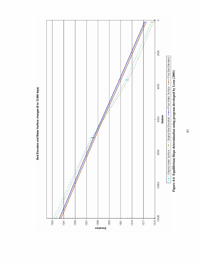
83
�Fi
gure
4-6
Equ
ilibr
ium
Slo
pe d
eter
min
atio
n us
ing
prog
ram
dev
elop
ed b
y L
eon
(200
1)
84
In addition, the model had a fourth upstream “dummy” reach to represent upstream
conditions that would take the place of Cochiti Dam. Without this reach, the upstream part of the
bed would not have been allowed to degrade.
Equilibrium Slopes Reach Water Bed
subreach 1 0.001261 0.001261 subreach 2 0.001287 0.001297 subreach 3 0.001234 0.001224 total reach 0.001258 0.001256
Table 4-7 Equilibrium slopes predicted by Leon’s (2001) model
4.3.3 Hydraulic Geometry
The equilibrium widths predicted by the hydraulic geometry equations for HEC-RAS
model data run at 5,000 cfs are summarized in Table 4-8 and displayed graphically in Figure 4-7.
Simons and Albertson’s, Julien-Wargadalam’s and Lacey’s equations all underestimate the width
for all subreaches for all years. Blench’s equation overestimates the width for all subreaches in
1962 and 1972, but predicts widths fairly closely to the observed values in 1992 and 2002.
Nouh’s equation vastly overestimates the width for all subreaches in 1962 and 1972, and also
greatly underestimates the widths for all subreaches in 1992 and 2002. Klassen and Vermeer’s
equation overestimates the width for all subreaches for all years analyzed.
From Figure 4-9, Blench’s 1992 and 2002 calculations produce width values close to the
channel width obtained by HEC-RAS analysis. The most accurate regime equations are from
Julien-Wargadalam, which underpredicts the HEC-RAS values. Overall, the regime equations
tend to inaccurately predict historical widths. However, they correctly predict little change in
channel width with time, as observed in this reach since the 1960’s. The Julien-Wargadalam,
Simons and Albertson, and Lacey equations also predict that the channel is becoming close to
equilibrium with time. This is indicated by the movement of the predicted widths towards the 1:1
line with observed widths.
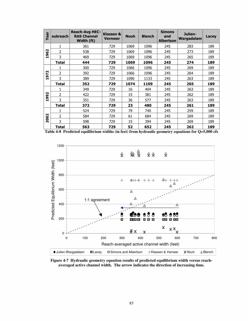
85
�����
��������
������!��"#��
�����������$����%&'�
(�� ���)�
*��+����,��� �������
��+� �
��������� ��
-������
$��������+�.���/�
� �� ���� ���� ���� �� � �� � ���
�� �� ���� ���� ���� �� � �� � ���
� ���� ���� ���� ���� �� � �� � ���0123�
4��� 555� 631� 0721� 0712� 358� 365� 091�
� ��� ���� ���� ���� �� � ���� ���
�� ��� ���� ���� ���� �� � ���� ���
� ��� ���� ���� � �� � �� � ���0163�
4��� :83� 631� 0765� 0071� 358� 328� 091�
� ��� ���� �� ���� �� � �� � ���
�� ���� ���� � �� �� � ���� ���
� � ���� �� ��� �� � �� � ���0113�
4��� :63� 631� 3:� 597� 358� 320� 091�
� ��� ���� ��� ���� �� � � �� ���
�� ��� ���� �� ���� �� � ���� ���
� ��� ���� � ��� �� � ���� ���3773�
4��� 82:� 631� 83� 283� 358� 323� 091�
Table 4-8 Predicted equilibrium widths (in feet) from hydraulic geometry equations for Q=5,000 cfs
0
200
400
600
800
1000
1200
0 100 200 300 400 500 600 700 800
Reach-averaged active channel width (feet)
Pre
dict
ed E
quili
briu
m W
idth
(fee
t)
Julien-Wargadalam Lacey Simons and Albertson Klassen & Vemeer Nouh Blench
1:1 agreement
�Figure 4-7 Hydraulic geometry equation results of predicted equilibrium width versus reach-
averaged active channel width. The arrow indicates the direction of increasing time.
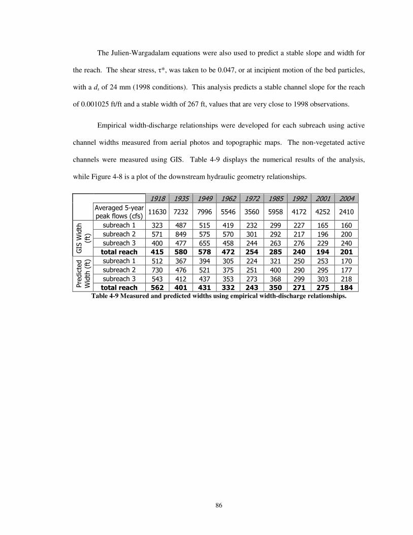
86
The Julien-Wargadalam equations were also used to predict a stable slope and width for
the reach. The shear stress, �*, was taken to be 0.047, or at incipient motion of the bed particles,
with a ds of 24 mm (1998 conditions). This analysis predicts a stable channel slope for the reach
of 0.001025 ft/ft and a stable width of 267 ft, values that are very close to 1998 observations.
Empirical width-discharge relationships were developed for each subreach using active
channel widths measured from aerial photos and topographic maps. The non-vegetated active
channels were measured using GIS. Table 4-9 displays the numerical results of the analysis,
while Figure 4-8 is a plot of the downstream hydraulic geometry relationships.
�� �� ��� � � ���� ���� ���� �� � ���� ���� �����
��
!(�$�.�/� �8��$�
���7�*���&�0�*&1�� �� �� �� ����� ��� ��� � �� ���� �� �� ����
&"�$������ � � ���� � ��� � �� ���� ���� � � ���
&"�$������� �� ���� � � ��� �� ���� ��� ��� ����
&"�$����� � ���� ���� � � � �� ���� �� � ���� ���� ����
�9��3
/���
0*�1�
��������� 508� 897� 869� 563� 385� 398� 357� 015� 370�
&"�$������ �� ��� ��� � � ���� �� � �� � � ���
&"�$������� � �� ���� �� � � � � ���� ���� �� � ���
&"�$����� � � � ��� � �� � �� � ��� ���� � � ���
:$�/���/�
3/���0*�1�
��������� 823� 570� 5:0� ::3� 35:� :87� 360� 368� 095�Table 4-9 Measured and predicted widths using empirical width-discharge relationships.
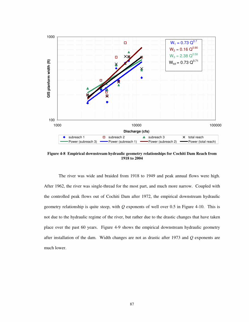
87
100
1000
1000 10000 100000
Discharge (cfs)
GIS
pla
nfor
m w
idth
(ft)
subreach 1 subreach 2 subreach 3 total reachPower (subreach 3) Power (subreach 1) Power (subreach 2) Power (total reach)
W1 = 0.73 Q0.7
W2 = 0.16 Q0.90
W3 = 2.38 Q0.58
Wtot = 0.73 Q0.71
�Figure 4-8 Empirical downstream hydraulic geometry relationships for Cochiti Dam Reach from
1918 to 2004
The river was wide and braided from 1918 to 1949 and peak annual flows were high.
After 1962, the river was single-thread for the most part, and much more narrow. Coupled with
the controlled peak flows out of Cochiti Dam after 1972, the empirical downstream hydraulic
geometry relationship is quite steep, with Q exponents of well over 0.5 in Figure 4-10. This is
not due to the hydraulic regime of the river, but rather due to the drastic changes that have taken
place over the past 60 years. Figure 4-9 shows the empirical downstream hydraulic geometry
after installation of the dam. Width changes are not as drastic after 1973 and Q exponents are
much lower.
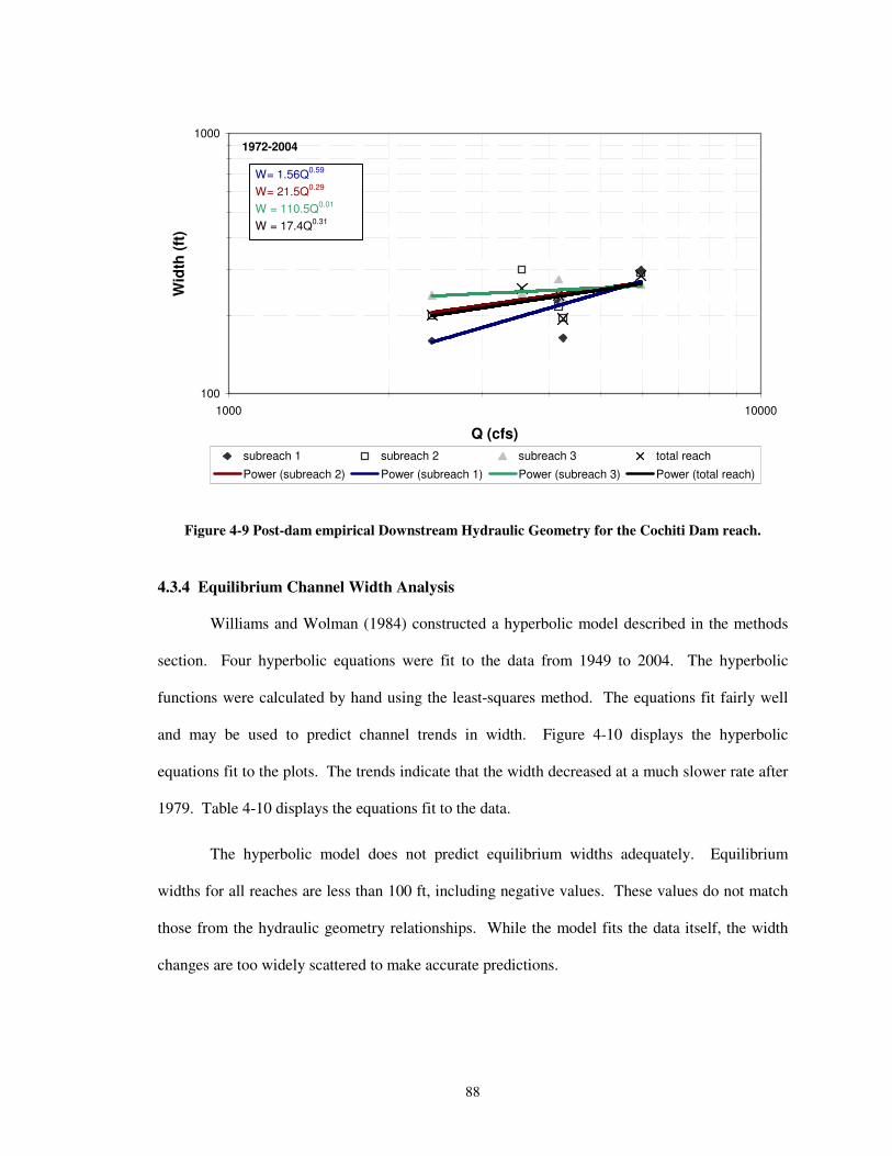
88
1972-2004
100
1000
1000 10000
Q (cfs)
Wid
th (f
t)
subreach 1 subreach 2 subreach 3 total reach
Power (subreach 2) Power (subreach 1) Power (subreach 3) Power (total reach)
W= 1.56Q0.59
W= 21.5Q0.29
W = 110.5Q0.01
W = 17.4Q0.31
�Figure 4-9 Post-dam empirical Downstream Hydraulic Geometry for the Cochiti Dam reach.
�
4.3.4 Equilibrium Channel Width Analysis
Williams and Wolman (1984) constructed a hyperbolic model described in the methods
section. Four hyperbolic equations were fit to the data from 1949 to 2004. The hyperbolic
functions were calculated by hand using the least-squares method. The equations fit fairly well
and may be used to predict channel trends in width. Figure 4-10 displays the hyperbolic
equations fit to the plots. The trends indicate that the width decreased at a much slower rate after
1979. Table 4-10 displays the equations fit to the data.
The hyperbolic model does not predict equilibrium widths adequately. Equilibrium
widths for all reaches are less than 100 ft, including negative values. These values do not match
those from the hydraulic geometry relationships. While the model fits the data itself, the width
changes are too widely scattered to make accurate predictions.
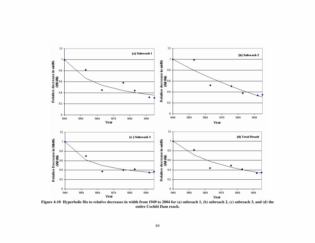
89
�Figure 4-10 Hyperbolic fits to relative decreases in width from 1949 to 2004 for (a) subreach 1, (b) subreach 2, (c) subreach 3, and (d) the
entire Cochiti Dam reach.

90
�Table 4-10 Hyperbolic fits to relative width plots using least-squares method.
�
Richard’s (2001) exponential model was fitted to the observed active channel width data
from aerial photos and topographic surveys of the Cochiti Dam reach. The k1 and We values were
estimated using methods 1 and 2. Due to the inexact results from the hydraulic geometry
equations, method 3 was not implemented.
Figure 4-11 shows the results of method 1. Change in active channel width was plotted
against active channel width to estimate the initial k1 and We values. Table 4-11 summarizes the
results. Method 2 produced very similar results with a slightly higher degree of accuracy. In this
method, the value of We was varied until the sum of the square of errors was minimized between
We and the observed width. The results are shown in Table 4-12 and a plot of the results of
methods 1 and 2 is shown in Figure 4-14. The exponential equations produced by methods 1 and
2 are summarized in Tables 4-13 and 4-14.
Richard’s model computes an exponential line from the first data point in 1949. Because
the widths in the Cochiti Dam reach vary so widely from year to year, this method does not make
a best-fit estimate for all the data points. For this reason, a Best Engineering Estimate fit was also
applied visually. The fits and resulting equations are shown in Figure 4.12, Table 4.13, and Table
14.
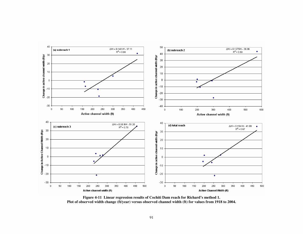
91
�Figure 4-11 Linear regression results of Cochiti Dam reach for Richard’s method 1.
Plot of observed width change (ft/year) versus observed channel width (ft) for values from 1918 to 2004.
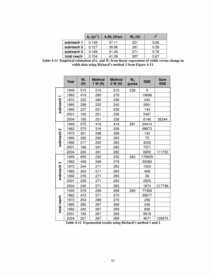
92
�
k1 (yr-1) k1We (ft/yr) We (ft) r2
subreach 1 0.148 37.11 251 0.66 subreach 2 0.127 36.96 291 0.59 subreach 3 0.189 51.26 271 0.78 total reach 0.154 41.09 267 0.67
Table 4-11 Empirical estimation of k1 and We from linear regressions of width versus change in width data using Richard’s method 1 from Figure 4-11.
��
Year Wt
(ft) Method 1 W (ft)
Method 2 W (ft)
We guess SSE Sum
SSE
1949 515 515 515 238 0 1962 419 289 279 19686 1972 232 260 248 240 1985 299 252 240 3561 1992 227 251 239 143 2001 165 251 238 5467 su
brea
ch 1
2004 160 251 238 6146 35244 1949 575 419 419 281 24414 1962 570 316 308 68873 1972 301 298 289 142 1985 292 292 283 75 1992 217 292 282 4225 2001 196 291 282 7371 su
brea
ch 2
2004 200 291 282 6650 111750 1949 655 232 232 283 178929 1962 458 268 279 32080 1972 244 271 283 1523 1985 263 271 283 409 1992 276 271 283 59 2001 229 271 283 2925 su
brea
ch 3
2004 240 271 283 1874 217798 1949 578 299 299 269 77469 1962 472 271 273 39577 1972 254 268 270 256 1985 285 267 269 246 1992 240 267 269 836 2001 194 267 269 5618 tota
l rea
ch
2004 201 267 269 4671 128674 Table 4-12 Exponential results using Richard’s method 1 and 2
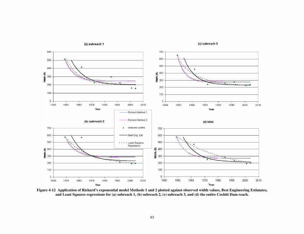
93
�Figure 4-12 Application of Richard’s exponential model Methods 1 and 2 plotted against observed width values, Best Engineering Estimates,
and Least Squares regressions for (a) subreach 1, (b) subreach 2, (c) subreach 3, and (d) the entire Cochiti Dam reach.
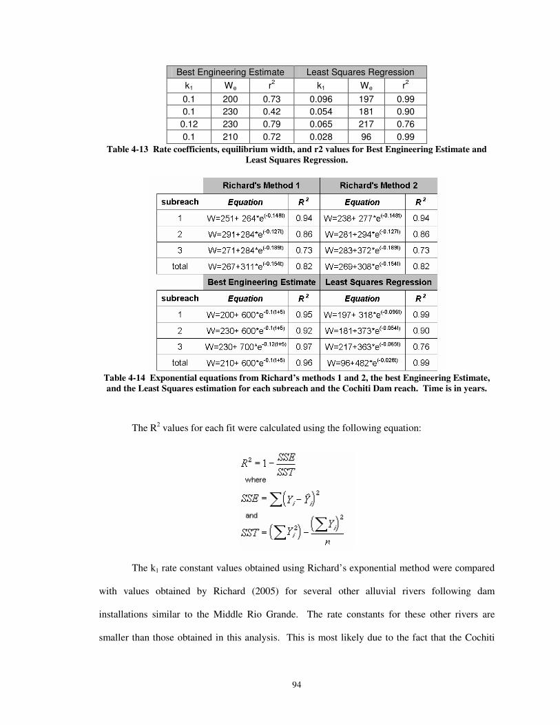
94
Best Engineering Estimate Least Squares Regression k1 We r2 k1 We r2 0.1 200 0.73 0.096 197 0.99 0.1 230 0.42 0.054 181 0.90 0.12 230 0.79 0.065 217 0.76 0.1 210 0.72 0.028 96 0.99
Table 4-13 Rate coefficients, equilibrium width, and r2 values for Best Engineering Estimate and Least Squares Regression.
Table 4-14 Exponential equations from Richard’s methods 1 and 2, the best Engineering Estimate, and the Least Squares estimation for each subreach and the Cochiti Dam reach. Time is in years.
The R2 values for each fit were calculated using the following equation:
����
The k1 rate constant values obtained using Richard’s exponential method were compared
with values obtained by Richard (2005) for several other alluvial rivers following dam
installations similar to the Middle Rio Grande. The rate constants for these other rivers are
smaller than those obtained in this analysis. This is most likely due to the fact that the Cochiti
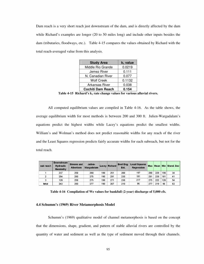
95
Dam reach is a very short reach just downstream of the dam, and is directly affected by the dam
while Richard’s examples are longer (20 to 50 miles long) and include other inputs besides the
dam (tributaries, floodways, etc.). Table 4-15 compares the values obtained by Richard with the
total reach-averaged value from this analysis.
Study Area k1 value Middle Rio Grande 0.0219
Jemez River 0.111 N. Canadian River 0.077
Wolf Creek 0.1132 Arkansas River 0.038
Cochiti Dam Reach 0.154 Table 4-15 Richard’s k1 rate change values for various alluvial rivers.
All computed equilibrium values are compiled in Table 4-16. As the table shows, the
average equilibrium width for most methods is between 200 and 300 ft. Julien-Wargadalam’s
equations predict the highest widths while Lacey’s equations predict the smallest widths.
William’s and Wolman’s method does not predict reasonable widths for any reach of the river
and the Least Squares regression predicts fairly accurate widths for each subreach, but not for the
total reach.
Table 4-16 Compilation of We values for bankfull (2-year) discharge of 5,000 cfs. �
4.4 Schumm’s (1969) River Metamorphosis Model
�Schumm’s (1969) qualitative model of channel metamorphosis is based on the concept
that the dimensions, shape, gradient, and pattern of stable alluvial rivers are controlled by the
quantity of water and sediment as well as the type of sediment moved through their channels.
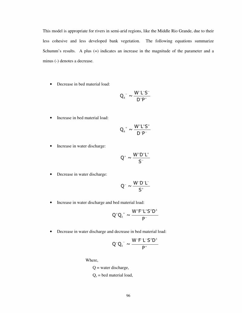
96
This model is appropriate for rivers in semi-arid regions, like the Middle Rio Grande, due to their
less cohesive and less developed bank vegetation. The following equations summarize
Schumm’s results. A plus (+) indicates an increase in the magnitude of the parameter and a
minus (-) denotes a decrease.
�
• Decrease in bed material load:
++
−−−−
:�
�;3<5&
• Increase in bed material load:
−−
++++
:�
�;3<5&
• Increase in water discharge:
−
++++
�
;�3<5
• Decrease in water discharge:
+
−−−−
�
;�3<5
• Increase in water discharge and bed material load:
−
±±+++++
:
��;�3<55 �
• Decrease in water discharge and decrease in bed material load:
+
±±−−−−−
:
��;�3<55 �
Where,
Q = water discharge,
Qs = bed material load,
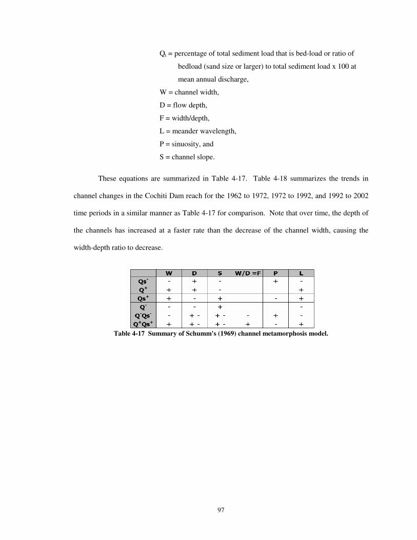
97
Qt = percentage of total sediment load that is bed-load or ratio of
bedload (sand size or larger) to total sediment load x 100 at
mean annual discharge,
W = channel width,
D = flow depth,
F = width/depth,
L = meander wavelength,
P = sinuosity, and
S = channel slope.
These equations are summarized in Table 4-17. Table 4-18 summarizes the trends in
channel changes in the Cochiti Dam reach for the 1962 to 1972, 1972 to 1992, and 1992 to 2002
time periods in a similar manner as Table 4-17 for comparison. Note that over time, the depth of
the channels has increased at a faster rate than the decrease of the channel width, causing the
width-depth ratio to decrease.
Table 4-17 Summary of Schumm's (1969) channel metamorphosis model.
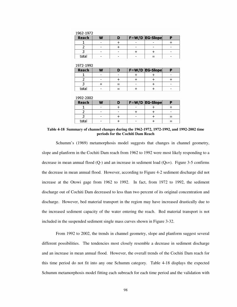
98
�Table 4-18 Summary of channel changes during the 1962-1972, 1972-1992, and 1992-2002 time
periods for the Cochiti Dam Reach
Schumm’s (1969) metamorphosis model suggests that changes in channel geometry,
slope and planform in the Cochiti Dam reach from 1962 to 1992 were most likely responding to a
decrease in mean annual flood (Q-) and an increase in sediment load (Qs+). Figure 3-5 confirms
the decrease in mean annual flood. However, according to Figure 4-2 sediment discharge did not
increase at the Otowi gage from 1962 to 1992. In fact, from 1972 to 1992, the sediment
discharge out of Cochiti Dam decreased to less than two percent of its original concentration and
discharge. However, bed material transport in the region may have increased drastically due to
the increased sediment capacity of the water entering the reach. Bed material transport is not
included in the suspended sediment single mass curves shown in Figure 3-32.
From 1992 to 2002, the trends in channel geometry, slope and planform suggest several
different possibilities. The tendencies most closely resemble a decrease in sediment discharge
and an increase in mean annual flood. However, the overall trends of the Cochiti Dam reach for
this time period do not fit into any one Schumm category. Table 4-18 displays the expected
Schumm metamorphosis model fitting each subreach for each time period and the validation with
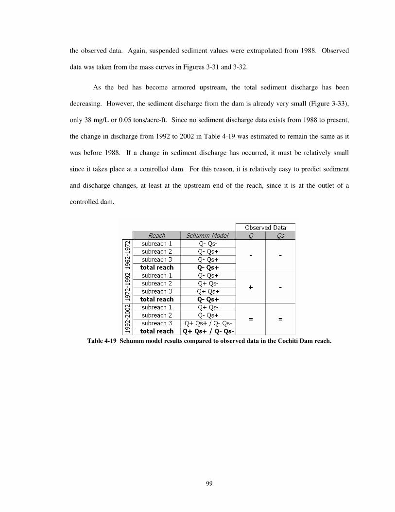
99
the observed data. Again, suspended sediment values were extrapolated from 1988. Observed
data was taken from the mass curves in Figures 3-31 and 3-32.
As the bed has become armored upstream, the total sediment discharge has been
decreasing. However, the sediment discharge from the dam is already very small (Figure 3-33),
only 38 mg/L or 0.05 tons/acre-ft. Since no sediment discharge data exists from 1988 to present,
the change in discharge from 1992 to 2002 in Table 4-19 was estimated to remain the same as it
was before 1988. If a change in sediment discharge has occurred, it must be relatively small
since it takes place at a controlled dam. For this reason, it is relatively easy to predict sediment
and discharge changes, at least at the upstream end of the reach, since it is at the outlet of a
controlled dam.
�Table 4-19 Schumm model results compared to observed data in the Cochiti Dam reach.
�
�
�
�
�
�
100
Chapter 5: Summary and Conclusions
The morphologic analysis of the Cochiti Dam reach of the Middle Rio Grande entailed a
detailed examination of channel characteristics including geometry, planform, and bed material.
Discharge and suspended sediment were also studied and were input into several modeling
programs for further analysis.
5.1 Summary
Discharge – Total annual discharge at the Cochiti gage decreased after 1950 to two-thirds
of its previous annual discharge from 1931 to 1950 (see Figure 4-1). After 1978, the total annual
discharge increased again by a factor of 1.5. Factors such as dam management, climate changes,
irrigation and other water diversions may be responsible for these changes.
Suspended Sediment – The total annual suspended sediment discharge at the Cochiti gage
reveals staunch evidence of the trap efficiency of the dam (see Figure 3-32). After the dam was
installed, the suspended sediment discharge exiting the dam dropped to 2% of its original
concentration at Otowi gage.
Bed Material – The median bed material at the Cochiti Dam gage was fine to medium
sand in 1970, very coarse sand to coarse gravel in 1980, and coarse gravel to very coarse gravel in
1998 (refer to Table 3-11).
Coarsening of the bed sediments increased overall with distance downstream and with
time. The median grain size was sand until the dam was built. Armoring clearly began with the
101
appearance of gravel as the median sediment size in the mid 1970s. Subreach 1 generally had bed
sediment trends that were representative of the entire reach.
Channel pattern – From GIS analysis, the overall trend of the channel from 1918 to 2004
has been a narrowing of the width and a shift from a braided to meandering planform. According
to the width measurements from the digitized aerial photos, the overall width of the reach
increased from 1918 to 1949, drastically decreased after 1949 to 1973, and then decreased
slightly from 1973 to 2004. This finding is supported by the HEC-RAS modeling results from
1973 to 2002. This suggests that the channelization efforts beginning in the 1930s may have had
more of an impact on the river than the dam itself. Average sinuosity increased slightly from
1.20 in 1918 to 1962 and decreased from 1962 to 2004 from 1.21 to 1.13.
Channel Classification – The channel classification methods produced mixed results.
From the 1962 planforms, Lane, Henderson, and van den Berg’s methods were most accurate.
They described the channel as braided, which can be verified by the aerial photos. Van den
Berg’s method also described the channel as low sinuosity, which can be verified by the sinuosity
trends seen in Figure 3-10. After 1962, the channel appeared to be narrowing and becoming
mostly single-thread. For these years, Ackers and Charlton, Rosgen, and Parker produced
accurate results. They predicted meandering channels for each subreach and the total reach. Van
den Berg also predicted that the channel would be single-thread. Overall, van den Berg’s method
produced the most complete and accurate representation of the Cochiti Dam reach from 1962 to
2004.
Vertical Movement – Thalweg analysis was done on CO-lines 2 through 8. The
thalweg degraded over almost every CO-line in the reach between 1 and 3 feet from 1962 to
2002. Thalweg analysis from 1962 to 2002 demonstrated a degradation of almost 3 feet at CO-5
and an aggradation of almost 2 feet just upstream at CO-4. The aggradation here may be due to
102
an overbank area (Figure 3-24). With the exclusion of CO-4, the average reach degradation was
2.15 feet.
Based on mean bed elevations from Agg/Deg surveys, the mean bed elevation degraded
slightly after 1962, but began aggrading in the 1970s. Total mean bed degradation from 1962 to
1972 averaged over the entire reach was approximately one third of a foot. Mean bed elevation
increase in the reach from 1972 to 2002 totaled about one-half of a foot. Further analysis of the
discrepancy between thalweg degradation and mean bed aggradation led to the conclusion that
the “aggradation” seen in the agg/deg range-lines are most likely average mean bed elevation
changes due to a channel geometry change, not of actual aggradation in the channel bed.
Channel Geometry – General trends in channel geometry are summarized in Table 5-1.
The changes are summarized for each subreach and the total reach. Note that a plus (+) indicates
an increase in parameter value, a negative (-) denotes a decrease, and an equality (=) indicates no
change. Overall from 1962 to 2002, there was a decrease in width, area, width/depth ratio and
wetted perimeter. There was an increase in energy grade slope, velocity, depth, Froude number,
and water surface slope.
From GIS coverages, the width changes are similar to those modeled in HEC-RAS.
From digitized aerial photos, the width increased from 1918 to 1949, decreased drastically from
1949 to 1972, increased slightly from 1972 to 1985, and finally decreased slightly from 1985 to
2004 (see Figure 3-26). From the analysis of width and depth trends, it appears that most
narrowing of the channel occurred before the dam. The dam may act as a control, which may
have kept the channel at the relatively the same width for the last few decades.
Overbank Flow/Channel Capacity – Based on the HEC-RAS modeling results at a
discharge of 5,000 cfs, a small amount of overbank flow occurs in subreach 2 for all years (see
Figure 3-24). This may explain the aggradational trend seen at CO-4 (see Figure 3-7).
103
Equilibrium Predictors – Several predictors were used to estimate equilibrium and stable
conditions in the reach. Leon’s (2003) modeling program predicted an equilibrium slope much
shallower than the slopes observed in the reach (between 70% and 85% of the observed slopes).
Both Williams and Wolman (1984) and Richard’s (2001) models fit accurate decreasing trends to
the historic width-discharge data. None of the hydraulic geometry equations accurately predict
width; however, they accurately estimate unchanging width trends with time. Julien-
Wargadalam’s equations predict stable slope and width that are very close to those observed for
1998.
5.2 Conclusions
The hydraulic modeling of the Cochiti Dam reach on the Middle Rio Grande River, NM,
produced a detailed characterization of the river over space and time. The highly controlled
dam’s reduced flows and clearwater discharge induced major changes to the channel and its flow
regime.
The Middle Rio Grande Database was organized and updated for facilitation of this
analysis. The discharge, sediment, and geometric data in this database, in addition to the
numerous literature resources, were then compiled to analyze spatial and temporal trends in the
Cochiti Dam reach of the Middle Rio Grande River.
After the dam closure in 1973, floods were nearly eliminated since peak annual flows did
not exceed 10,000 cfs. The channel narrowed by 50 - 100 feet after the dam closure. Both
average width-depth ratio and cross-sectional area were reduced by a third and thalweg
degradation averaged 2 feet over the entire reach. Median bed sediment sizes jumped from an
average of 0.1 mm in 1962 to an average of 24 mm in 1998, armoring the bed. This was due to
the 98% decrease in suspended sediment after the dam construction. The changes in bed
sediment sizes are more apparent in subreach 1 than subreach 3, indicating a decrease of dam
effects with distance downstream. This is corroborated by outside analyses on downstream
104
reaches of the Middle Rio Grande. Overall, Cochiti dam had a much more noticeable effect on
bed sediment than channel geometry.
Equilibrium analysis of the reach using sediment transport functions, equilibrium channel
width and slope analysis, and regime equations suggested that the Cochiti Dam reach is moving
towards stable channel conditions and the channel may begin experiencing lateral motion, which
will begin eroding the banks.
�
�
�
�
�
�
�
�
�
�
�
�
�
�
�
�
�
�
105
References
Ackers, P. (1982). Meandering Channels and the Influence of Bed Material. Gravel Bed Rivers.
Fluvial Processes, Engineering and Management. Edited by R.D. Hey, J.C. Bathurst and C.R.Thorne. John Wiley & Sons Ltd. 389-414
Albert, J., Sixta, M., Leon, C., and Julien, P.Y. (2003). Corrales Reach. Corrales Flood Channel
to Montano Bridge. Hydraulic Modeling Analysis. 1962-2001. Middle Rio Grande, New Mexico. Prepared for U.S. Bureau of Reclamation. Albuquerque, New Mexico. Colorado State University, Fort Collins, CO.
Albert, J. (2004) Hydraulic Analysis and Double Mass Curves of the Middle Rio Grande from
Cochiti to San Marcial, New Mexico. M.S. Thesis. Colorado State University, Fort Collins, CO. 207 pp.
Baird, D. C. (1996). River Mechanics Experience on the Middle Rio Grande. 6th Federal
Interagency Sediment Conference. March 11-14. 8 pp. Bauer, T. R. (2000). Morphology of the Middle Rio Grande from Bernalillo Bridge to the San
Acacia Diversion Dam, New Mexico. M.S. Thesis. Colorado State University, Fort Collins, CO. 308 pp.
Blench, T. (1957). Regime Behaviour of Canals and Rivers. London: Butterworths Scientific
Publications. 138 pp. Bullard, K.L. and Lane, W.L. (1993). Middle Rio Grande Peak Flow Frequency Study. U.S.
Department of the Interior, Bureau of Reclamation, Albuquerque, NM. 36 pp. Burkholder, J.L., Report of the Chief Engineer. Middle Rio Grande Conservancy District.
Albuquerque, New Mexico. Dated March 19, 1929. Chang, H.H. (1979). Minimum Stream Power and River Channel Patterns. Journal of
Hydrology, 41, 303-327. Crawford, C.S., Culley, A.C., Leutheuser, R., Sifuentes, M.S., White, L.H., Wilber, J.P. (1993).
Middle Rio Grande Ecosystem: Bosque Biological Management Plan. U.S. Fish and Wildlife Service, Albuquerque, New Mexico.
Dewey, J.D., Roybal, F.E., Funderburg, D.E., (1979). Hydraulic Data on Channel Adjustments
1970 to 1975, on the Rio Grande Downstream from Cochiti Dam, New Mexico Before and After Closure. U.S. Geological Survey, Water Resources Investigations.
Graf, W.L. (1994). Plutonium and the Rio Grande. Environmental Change and Contamination
in the Nuclear Age. New York : Oxford University Press. Henderson, F.M. (1966). Open Channel Flow. New York, NY : Macmillan Publishing Co., Inc.
106
Hereford, R., (1984) Climate and ephemeral-stream processes: Twentieth-century geomorphology and alluvial stratigraphy of the Little Colorado River, Arizona. Geological Society of America Bulletin, v. 95, p. 654-668.
Holmquist-Johnson, C. (2005) Personal Communication. Hydraulic Engineer. Representing U.S.
Bureau of Reclamation, Sedimentation and Hydraulics Group. Denver, CO. Julien, P.Y. (1995) Erosion and Sedimentation. New York, NY: Cambridge University Press. 280
pp. Julien, P.Y. (1998) River Mechanics. New York, NY: Cambridge University Press. 434 pp. Julien, P.Y. and Wargadalam, J. (1995). Alluvial Channel Geometry: Theory and Applications.
Journal of Hydraulic Engineering, 121(4), 312-325. Klaassen, G.J. and Vermeer, K. (1988). Channel Characteristics of the Braiding Jamuna River,
Bangladesh. International Conference on River Regime, 18-20 May 1988. W.R. White (ed.), Hydraulics Research Ltd., Wallingford, UK. pp 173-189.
Knighton, A.D. and Nanson, G.C. (1993). Anastomosis and the Continuum of Channel Pattern.
Earth Surface Processes and Landforms, 18, 613-625. Lagasse, P.F. (1980). An Assessment of the Response of the Rio Grande to Dam Construction –
Cochiti to Isleta Reach. U.S. Army Corps of Engineers. Albuquerque, NM. Lagasse, P. F. (1994). Variable Response of the Rio Grande to Dam Construction, The
Variability of Large Alluvial Rivers. ASCE Press, New York, NY. Lane, E.W., Borland, W.M., (1953), River Bed Scour During Floods. Transactions, ASCE, Paper
No. 2712. Lane, E.W. (1955). The importance of fluvial morphology in hydraulic engineering. Proc.
ASCE, 81(745):1-17. Leon, C. (1998). Morphology of the Middle Rio Grande from Cochiti Dam to Bernalillo Bridge,
New Mexico. M.S. Thesis. Colorado State University, Fort Collins, CO. 210 pp. Leon, C. and Julien, P.Y. (2001a). Hydraulic Modeling on the Middle Rio Grande, NM.
Corrales Reach. Corrales Flood Channel to Montano Bridge. Prepared for U.S. Bureau of Reclamation. Albuquerque, New Mexico. Colorado State University, Fort Collins, CO. 83 pp.
Leon, C. and Julien, P.Y. (2001b). Bernalillo Bridge Reach. Highway 44 Bridge to Corrales
Flood Channel Outfall. Hydraulic Modeling Analysis. 1962-1992. Middle Rio Grande, New Mexico. Prepared for the U.S. Bureau of Reclamation. Albuquerque, New Mexico. Colorado State University, Fort Collins, CO. 85 pp.
Leon, C. (2003). Analysis of Equivalent Widths of Alluvial Channels and Application for
Instream Habitat in the Rio Grande. Ph.D. Dissertation. Colorado State University, Fort Collins, CO. 308 pp.
107
Leopold, L.B. and Maddock, T. Jr. (1953). The Hydraulic Geometry of Stream Channels and Some Physiographic Implications. USGS Professional Paper 252, 57 pp.
Leopold, L.B. and Wolman, M.G. (1957). River Channel Patterns: Braided, Meandering and
Straight, USGS Professional Paper 282-B. 85 pp. Mackin, J. H. (1948). Concept of the graded river. Geol. Soc. Am. Bull., 59:463-512 Mosley, J. and Boelman, S. (1998). Santa Ana Reach. Geomorphic Report – Draft. U.S. Bureau
of Reclamation, Albuquerque, NM. Nanson, G.C. and Croke, J.C. (1992). A genetic classification of floodplains. Geomorphology. 4,
459-486. New Mexico Culturenet. The science of the river. Available at:
http://www.nmculturenet.org/heritage/river/pdf_files/science/day_nine_science.pdf. Accessed August 3, 2005.
Nordin, C.F. Jr., Beverage, J.P., (1965) Sediment Transport in the Rio Grande, New Mexico,
USGS Professional Paper 462-F. Nouh, M. (1988). Regime Channels of an Extremely Arid Zone. International Conference on
River Regime, 18-20 May 1988. W.R. White (ed.). Hydraulics Research Ltd., Wallingford, UK. pp 55-66.
Novak, S.J., Julien, P.Y. (2005 draft). Cochiti Dam Reach. Cochiti Dam to Galisteo Creek.
Hydraulic Modeling Analysis. 1962-2002. Middle Rio Grande, New Mexico. Prepared for U.S. Bureau of Reclamation. Albuquerque, New Mexico. Colorado State University, Fort Collins, CO.
Ortiz, R.M., Meyer, G.A. Downstream Effects of Cochiti Dam on the Middle Rio Grande and the
Channel Transition Zone near Albuquerque, New Mexico. 2005 Salt Lake City Annual Meeting, Geological Society of America, Paper No. 145-3.
Parker, G. (1976). On the Cause and Characteristic Scales of Meandering and Braiding in Rivers.
Journal of Fluid Mechanics, vl. 76, part 3, pp 457-480. Pueblo de Cochiti Farm Enterprise. The Official Web site of the Cochiti Pueblo. Available at:
http://www.pueblodecochiti.org/farm.html. Accessed August 2, 2005. Richard, G., Leon, C., and Julien, P.Y. (2001). Hydraulic Modeling on the Middle Rio Grande,
New Mexico. Rio Puerco Reach. Prepared for U.S. Bureau of Reclamation. Albuquerque, New Mexico. Colorado State University, Fort Collins, CO.
Richard, G. (2001). Quantification and Prediction of Lateral Channel Adjustments Downstream
from Cochiti Dam, Rio Grande, NM. Ph.D. Dissertation. Colorado State University, Fort Collins, CO. 244 pp.
Richard,G., Julien, P.Y., and Baird, D. (2005). Case Study: Modeling the Lateral Mobility of the
Rio Grande below Cochiti Dam, New Mexico. Journal of Hydraulic Engineering. Vol. 131 No. 11. pp. 931-941.
108
Richardson, E.V., Simons, D. B. and Julien, P.Y. (1990). Highways in the River Environment.
U.S. Department of Transportation. Federal Highway Administration. 610 pp. Rosgen, D. (1996). Applied River Morphology, Pagosa Springs, CO: Wildland Hydrology. 360
pp. Sanchez, V. and Baird, D. (1997). River Channel Changes Downstream of Cochiti Dam. Middle
Rio Grande, New Mexico. Proceedings of the Conference of Management of Landscapes Disturbed by Channel Incision. University of Mississippi, Oxford, MS.
Schembera, R.E., (1963). Development of Hydraulics and Sediment Transport Relationships and
Their Use for Channel Design of Middle Rio Grande Channelization. U.S. Bureau of Reclamation, Albuquerque, New Mexico.
Schumm, S.A. (1969). River Metamorphosis. Journal of the Hydraulics Division. Vol. 95, No. 1.
pp 255-273. Schumm, S. A. and Khan, H.R. (1972). Experimental Study of Channel Patterns. Geological
Society of America Bulletin, 83, 1755-1770. Scurlock, D. (1998). From the Rio to the Sierra. An Environmental History of the Middle Rio
Grande Basin. General Technical Report RMRS-GTR5. USDA, Forest Service, Rocky Mountain Research Station, Fort Collins, CO. 440 pp.
Simons, D.B. and Albertson, M.L. (1963). Uniform Water Conveyance Channels in Alluvial
Material. Transactions of the American Society of Civil Engineers. Paper No. 3399. Vol. 128, Part I. pp 65-107.
Sixta, M., Albert, J., Leon, C., and Julien, P.Y. (2003a). Bernalillo Bridge Reach. Highway 44
Bridge to Corrales Flood Channel Outfall. Hydraulic Modeling Analysis. 1962-2001. Middle Rio Grande, New Mexico. Prepared for U.S. Bureau of Reclamation. Albuquerque, New Mexico. Colorado State University, Fort Collins, CO. 87 pp.
Sixta, M., Albert, J., Leon, C., and Julien, P.Y. (2003b) San Felipe Reach. Arroyo Tonque to
Angostura Diversion Dam. Hydraulic Modeling Analysis. 1962-1998. Middle Rio Grande, New Mexico. Prepared for U.S. Bureau of Reclamation. Albuquerque, New Mexico. Colorado State University, Fort Collins, CO. 85 pp.
Sixta, M. (2004). Hydraulic Modeling and Meander Migration of the Middle Rio Grande, New
Mexico. M.S. Thesis. Colorado State University, Fort Collins, CO. 109 pp. U.S. Army Corps of Engineers, USACE (2002). HEC-RAS River Analysis System. User’s
Manual. v. 3.1. U.S. Army Corps of Engineers Institute for Water Resources. Hydrologic Engineering Center, Davis, CA.
U.S. Army Corps of Engineers, USACE (2005). Upper Rio Grande Water Operations Model
Physical Accounting Model Documentation. Retrieved September 15, 2005 from http://www.spa.usace.army.mil/urgwom/docintro.htm
109
U.S. Bureau of Reclamation, USBR. Middle Rio Grande Project Water Data. Available at http://www.usbr.gov/dataweb/html/ucmrgwatdata.html. Accessed September 1, 2005.
U.S. Geological Survey, USGS. Middle Rio Grande Basin Study. U.S. Department of the
Interior, U.S. Geological Survey, Albuquerque, NM. Available at http://nm.water.usgs.gov/mrg/index.htm. Accessed August 20, 2005.
Van den Berg, J.H. (1995). Prediction of Alluvial Channel Pattern of Perennial Rivers.
Geomorphology. 12, 259-279. Williams, G. and Wolman, G. (1984). Downstream Effects of Dams on Alluvial Rivers. U.S.
Geological Survey Professional Paper 1286, 83 pp. Wargadalam, J. (1993). Hydraulic Geometry of Alluvial Channels. Ph.D. Dissertation.
Colorado State University, Fort Collins, CO. 203 pp. Watson, C., Biedenharn, D., Thorne, C. (2005) Stream Rehabilitation. Cottonwood Research
LLC. Fort Collins, Colorado. 202pp. Woodson, R.C. (1961). Stabilization of the Middle Rio Grande in New Mexico. Proceedings of
the American Society of Civil Engineers. Journal of the Waterways and Harbor Division. 87:No. WW4: pp. 1-15
Woodson, R.C. and Martin, J.T. (1962). The Rio Grande Comprehensive Plan in New Mexico
and its Effects on the River Regime Through the Middle Valley. Control of Alluvial Rivers by Steel Jetties. Proceedings of the American Society of Civil Engineers. Journal of Waterways and Harbor Division. Carlson, E. J. and Dodge E. A. eds. American Society of Civil Engineers, New York, NY, 53-81.

110
A P P E N D I X A – A E R I A L P H O T O I N F OR M A T I O N
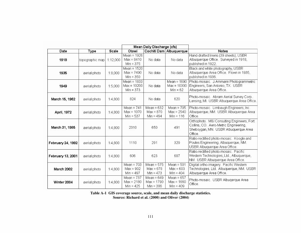
111
�Table A-1 GIS coverage source, scale, and mean daily discharge statistics.
Source: Richard et al. (2000) and Oliver (2004)
112
�
�
�
�
�
�
�
�
�
�
�
A P P E N D I X B – C R O S S - S E C T I O N P L OT S
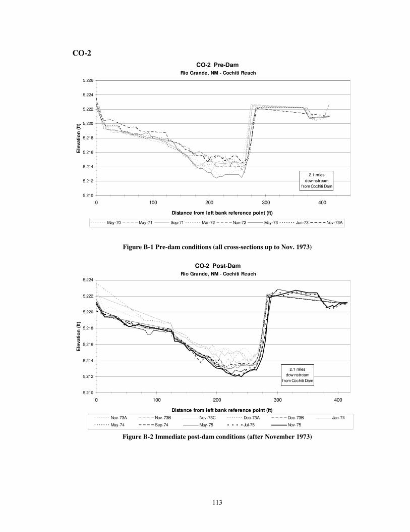
113
CO-2 CO-2 Pre-Dam
Rio Grande, NM - Cochiti Reach
5,210
5,212
5,214
5,216
5,218
5,220
5,222
5,224
5,226
0 100 200 300 400
Distance from left bank reference point (ft)
Ele
vatio
n (ft
)
May-70 May-71 Sep-71 Mar-72 Nov-72 May-73 Jun-73 Nov-73A
2.1 miles dow nstream
from Cochiti Dam
Figure B-1 Pre-dam conditions (all cross-sections up to Nov. 1973)
CO-2 Post-Dam Rio Grande, NM - Cochiti Reach
5,210
5,212
5,214
5,216
5,218
5,220
5,222
5,224
0 100 200 300 400
Distance from left bank reference point (ft)
Ele
vatio
n (ft
)
Nov-73A Nov-73B Nov-73C Dec-73A Dec-73B Jan-74
May-74 Sep-74 May-75 Jul-75 Nov-75
2.1 miles dow nstream
from Cochiti Dam
�Figure B-2 Immediate post-dam conditions (after November 1973)
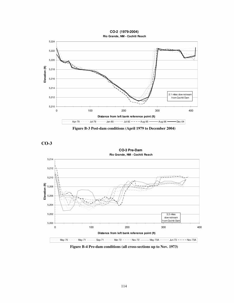
114
CO-2 (1979-2004) Rio Grande, NM - Cochiti Reach
5,210
5,212
5,214
5,216
5,218
5,220
5,222
5,224
0 100 200 300 400
Distance from left bank reference point (ft)
Ele
vatio
n (ft
)
Apr-79 Jul-79 Jan-80 Jul-92 Aug-95 Aug-98 Dec-04
2.1 miles dow nstream from Cochiti Dam
�Figure B-3 Post-dam conditions (April 1979 to December 2004)
�
CO-3 CO-3 Pre-Dam
Rio Grande, NM - Cochiti Reach
5,200
5,202
5,204
5,206
5,208
5,210
5,212
5,214
0 100 200 300 400
Distance from left bank reference point (ft)
Ele
vatio
n (ft
)
May-70 May-71 Sep-71 Mar-72 Nov-72 May-73A Jun-73 Nov-73A
3.3 miles dow nstream
from Cochiti Dam
�Figure B-4 Pre-dam conditions (all cross-sections up to Nov. 1973)
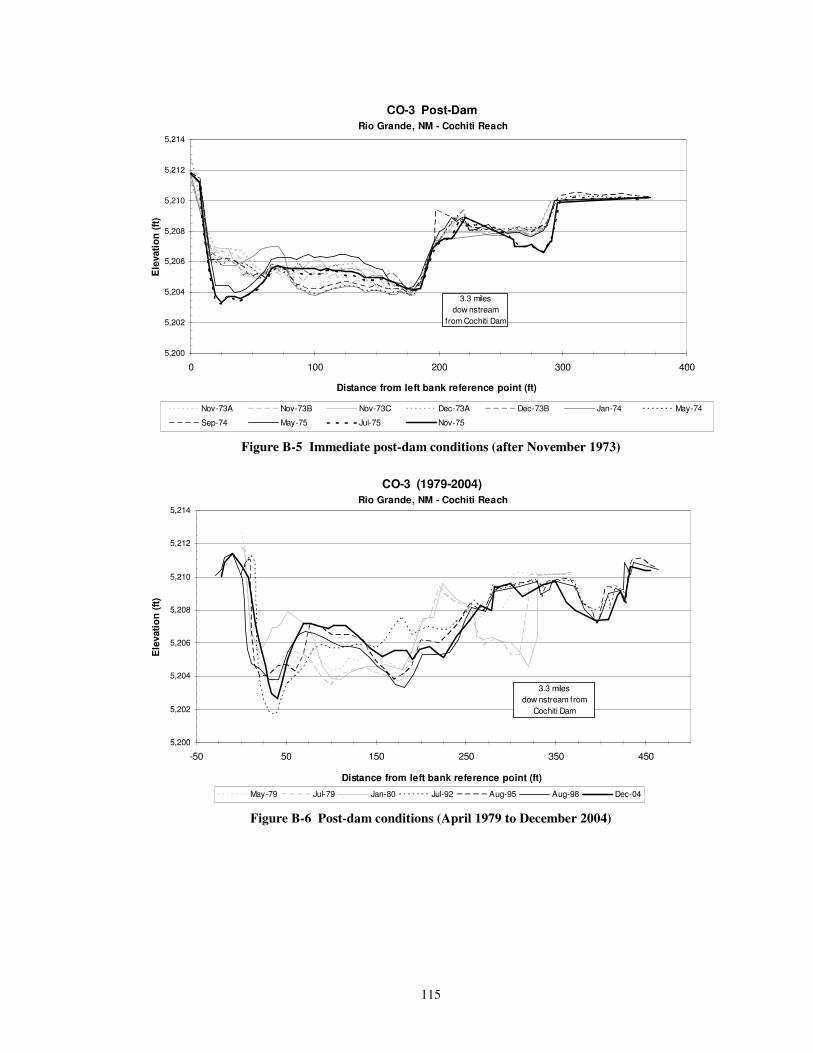
115
CO-3 Post-Dam Rio Grande, NM - Cochiti Reach
5,200
5,202
5,204
5,206
5,208
5,210
5,212
5,214
0 100 200 300 400
Distance from left bank reference point (ft)
Ele
vatio
n (ft
)
Nov-73A Nov-73B Nov-73C Dec-73A Dec-73B Jan-74 May-74
Sep-74 May-75 Jul-75 Nov-75
3.3 miles dow nstream
from Cochiti Dam
�Figure B-5 Immediate post-dam conditions (after November 1973)
CO-3 (1979-2004) Rio Grande, NM - Cochiti Reach
5,200
5,202
5,204
5,206
5,208
5,210
5,212
5,214
-50 50 150 250 350 450
Distance from left bank reference point (ft)
Ele
vatio
n (ft
)
May-79 Jul-79 Jan-80 Jul-92 Aug-95 Aug-98 Dec-04
3.3 miles dow nstream from
Cochiti Dam
�Figure B-6 Post-dam conditions (April 1979 to December 2004)
�
�
�
�
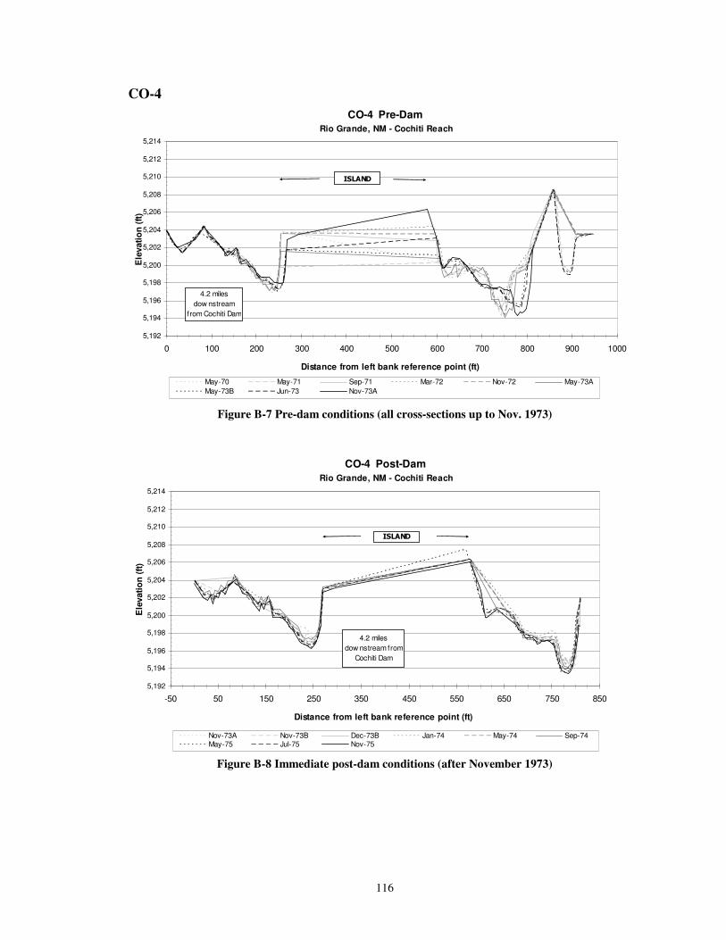
116
CO-4 CO-4 Pre-Dam
Rio Grande, NM - Cochiti Reach
5,192
5,194
5,196
5,198
5,200
5,202
5,204
5,206
5,208
5,210
5,212
5,214
0 100 200 300 400 500 600 700 800 900 1000
Distance from left bank reference point (ft)
Ele
vatio
n (ft
)
May-70 May-71 Sep-71 Mar-72 Nov-72 May-73AMay-73B Jun-73 Nov-73A
4.2 miles dow nstream
from Cochiti Dam
��.�,�
�Figure B-7 Pre-dam conditions (all cross-sections up to Nov. 1973)
CO-4 Post-Dam Rio Grande, NM - Cochiti Reach
5,192
5,194
5,196
5,198
5,200
5,202
5,204
5,206
5,208
5,210
5,212
5,214
-50 50 150 250 350 450 550 650 750 850
Distance from left bank reference point (ft)
Ele
vatio
n (ft
)
Nov-73A Nov-73B Dec-73B Jan-74 May-74 Sep-74May-75 Jul-75 Nov-75
4.2 miles dow nstream from
Cochiti Dam
��.�,�
�Figure B-8 Immediate post-dam conditions (after November 1973)
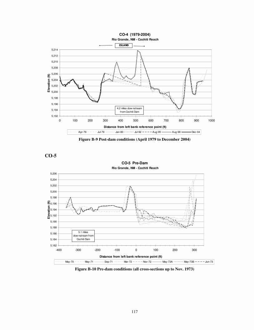
117
CO-4 (1979-2004) Rio Grande, NM - Cochiti Reach
5,192
5,194
5,196
5,198
5,200
5,202
5,204
5,206
5,208
5,210
5,212
5,214
0 100 200 300 400 500 600 700 800 900 1000
Distance from left bank reference point (ft)
Ele
vatio
n (ft
)
Apr-79 Jul-79 Jan-80 Jul-92 Aug-95 Aug-98 Dec-04
4.2 miles dow nstream from Cochiti Dam
��.�,�
�Figure B-9 Post-dam conditions (April 1979 to December 2004)
�
CO-5 CO-5 Pre-Dam
Rio Grande, NM - Cochiti Reach
5,182
5,184
5,186
5,188
5,190
5,192
5,194
5,196
5,198
5,200
5,202
5,204
5,206
-400 -300 -200 -100 0 100 200 300
Distance from left bank reference point (ft)
Ele
vatio
n (ft
)
May-70 May-71 Sep-71 Mar-72 Nov-72 May-73A May-73B Jun-73
5.1 miles dow nstream from
Cochiti Dam
�Figure B-10 Pre-dam conditions (all cross-sections up to Nov. 1973)
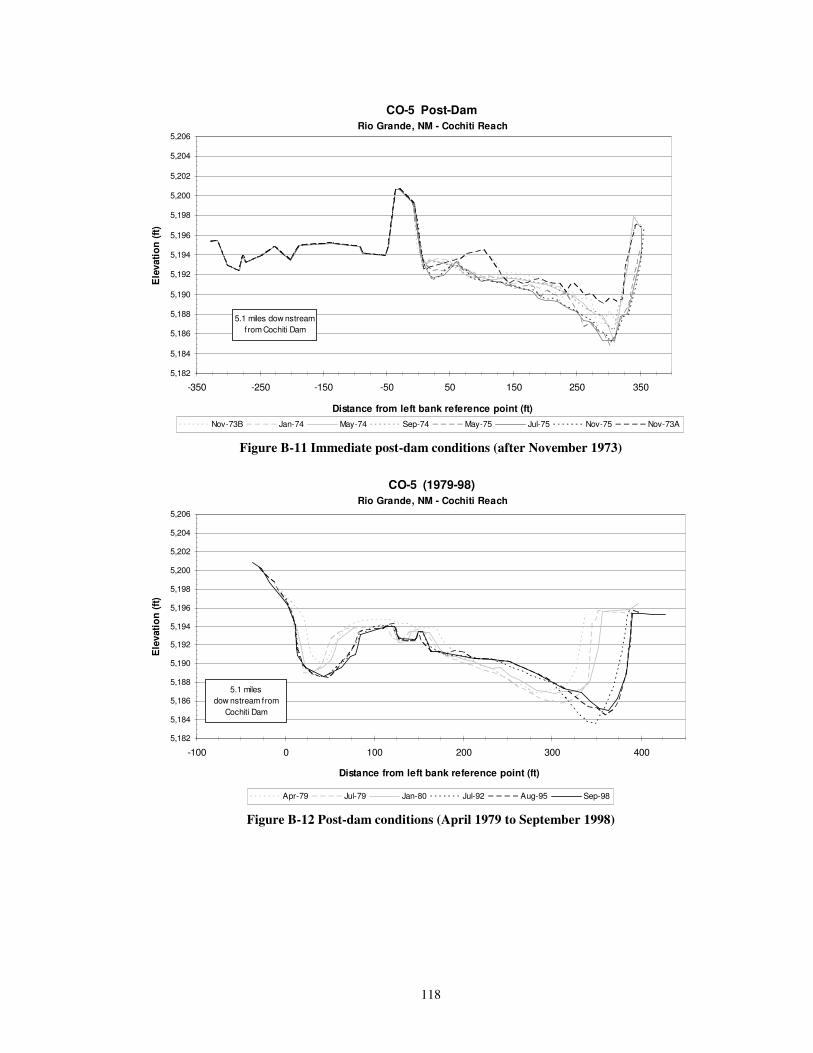
118
CO-5 Post-Dam Rio Grande, NM - Cochiti Reach
5,182
5,184
5,186
5,188
5,190
5,192
5,194
5,196
5,198
5,200
5,202
5,204
5,206
-350 -250 -150 -50 50 150 250 350
Distance from left bank reference point (ft)
Ele
vatio
n (ft
)
Nov-73B Jan-74 May-74 Sep-74 May-75 Jul-75 Nov-75 Nov-73A
5.1 miles dow nstream from Cochiti Dam
�Figure B-11 Immediate post-dam conditions (after November 1973)
CO-5 (1979-98) Rio Grande, NM - Cochiti Reach
5,182
5,184
5,186
5,188
5,190
5,192
5,194
5,196
5,198
5,200
5,202
5,204
5,206
-100 0 100 200 300 400
Distance from left bank reference point (ft)
Ele
vatio
n (ft
)
Apr-79 Jul-79 Jan-80 Jul-92 Aug-95 Sep-98
5.1 miles dow nstream from
Cochiti Dam
�Figure B-12 Post-dam conditions (April 1979 to September 1998)
�
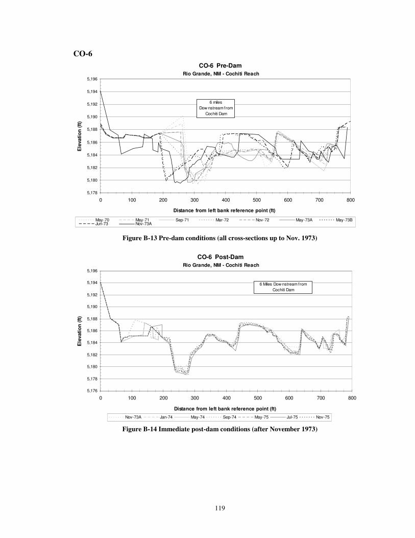
119
CO-6 CO-6 Pre-Dam
Rio Grande, NM - Cochiti Reach
5,178
5,180
5,182
5,184
5,186
5,188
5,190
5,192
5,194
5,196
0 100 200 300 400 500 600 700 800
Distance from left bank reference point (ft)
Ele
vatio
n (ft
)
May-70 May-71 Sep-71 Mar-72 Nov-72 May-73A May-73BJun-73 Nov-73A
6 miles Dow nstream from
Cochiti Dam
�Figure B-13 Pre-dam conditions (all cross-sections up to Nov. 1973)
CO-6 Post-Dam Rio Grande, NM - Cochiti Reach
5,176
5,178
5,180
5,182
5,184
5,186
5,188
5,190
5,192
5,194
5,196
0 100 200 300 400 500 600 700 800
Distance from left bank reference point (ft)
Ele
vatio
n (ft
)
Nov-73A Jan-74 May-74 Sep-74 May-75 Jul-75 Nov-75
6 Miles Dow nstream from Cochiti Dam
�Figure B-14 Immediate post-dam conditions (after November 1973)
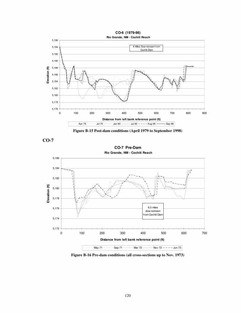
120
CO-6 (1979-98) Rio Grande, NM - Cochiti Reach
5,176
5,178
5,180
5,182
5,184
5,186
5,188
5,190
5,192
5,194
5,196
0 100 200 300 400 500 600 700 800 900
Distance from left bank reference point (ft)
Ele
vatio
n (ft
)
Apr-79 Jul-79 Jan-80 Jul-92 Aug-95 Sep-98
6 Miles Dow nstream from Cochiti Dam
�Figure B-15 Post-dam conditions (April 1979 to September 1998)
CO-7
CO-7 Pre-Dam Rio Grande, NM - Cochiti Reach
5,172
5,174
5,176
5,178
5,180
5,182
5,184
5,186
0 100 200 300 400 500 600 700
Distance from left bank reference point (ft)
Ele
vatio
n (ft
)
May-71 Sep-71 Mar-72 Nov-72 Jun-73
6.5 miles dow nstream
from Cochiti Dam
�Figure B-16 Pre-dam conditions (all cross-sections up to Nov. 1973)
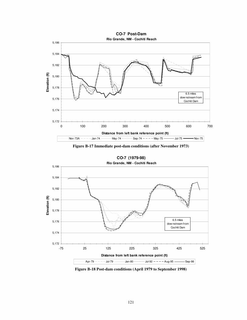
121
CO-7 Post-Dam Rio Grande, NM - Cochiti Reach
5,172
5,174
5,176
5,178
5,180
5,182
5,184
5,186
0 100 200 300 400 500 600 700
Distance from left bank reference point (ft)
Ele
vatio
n (ft
)
Nov-73A Jan-74 May-74 Sep-74 May-75 Jul-75 Nov-75
6.5 milesdow nstream from
Cochiti Dam
�Figure B-17 Immediate post-dam conditions (after November 1973)
CO-7 (1979-98) Rio Grande, NM - Cochiti Reach
5,172
5,174
5,176
5,178
5,180
5,182
5,184
5,186
-75 25 125 225 325 425 525
Distance from left bank reference point (ft)
Ele
vatio
n (ft
)
Apr-79 Jul-79 Jan-80 Jul-92 Aug-95 Sep-98
6.5 miles dow nstream from
Cochiti Dam
�Figure B-18 Post-dam conditions (April 1979 to September 1998)
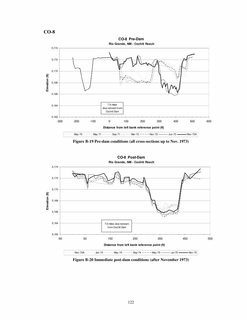
122
CO-8 CO-8 Pre-Dam
Rio Grande, NM - Cochiti Reach
5,162
5,164
5,166
5,168
5,170
5,172
5,174
-300 -200 -100 0 100 200 300 400 500 600
Distance from left bank reference point (ft)
Ele
vatio
n (ft
)
May-70 May-71 Sep-71 Mar-72 Nov-72 Jun-73 Nov-73A
7.6 miles dow nstream from
Cochiti Dam
�Figure B-19 Pre-dam conditions (all cross-sections up to Nov. 1973)
CO-8 Post-Dam Rio Grande, NM - Cochiti Reach
5,162
5,164
5,166
5,168
5,170
5,172
5,174
-50 50 150 250 350 450 550
Distance from left bank reference point (ft)
Ele
vatio
n (ft
)
Nov-73A Jan-74 May-74 Sep-74 May-75 Jul-75 Nov-75
7.6 miles dow nstream from Cochiti Dam
�Figure B-20 Immediate post-dam conditions (after November 1973)
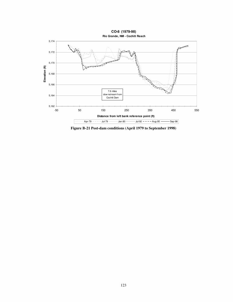
123
CO-8 (1979-98) Rio Grande, NM - Cochiti Reach
5,162
5,164
5,166
5,168
5,170
5,172
5,174
-50 50 150 250 350 450 550
Distance from left bank reference point (ft)
Ele
vatio
n (ft
)
Apr-79 Jul-79 Jan-80 Jul-92 Aug-95 Sep-98
7.6 miles dow nstream from
Cochiti Dam
�Figure B-21 Post-dam conditions (April 1979 to September 1998)
�
�
�
�
�
�
�
�
�
�
�
�
�
�
124
�
�
�
�
�
�
�
�
�
�
A P P E N D I X C – H E C - R A S H Y D R A U L I C G E O M E T R Y R E S U L T S
�
�
�
�
�
�
�
�
�
�
�
�
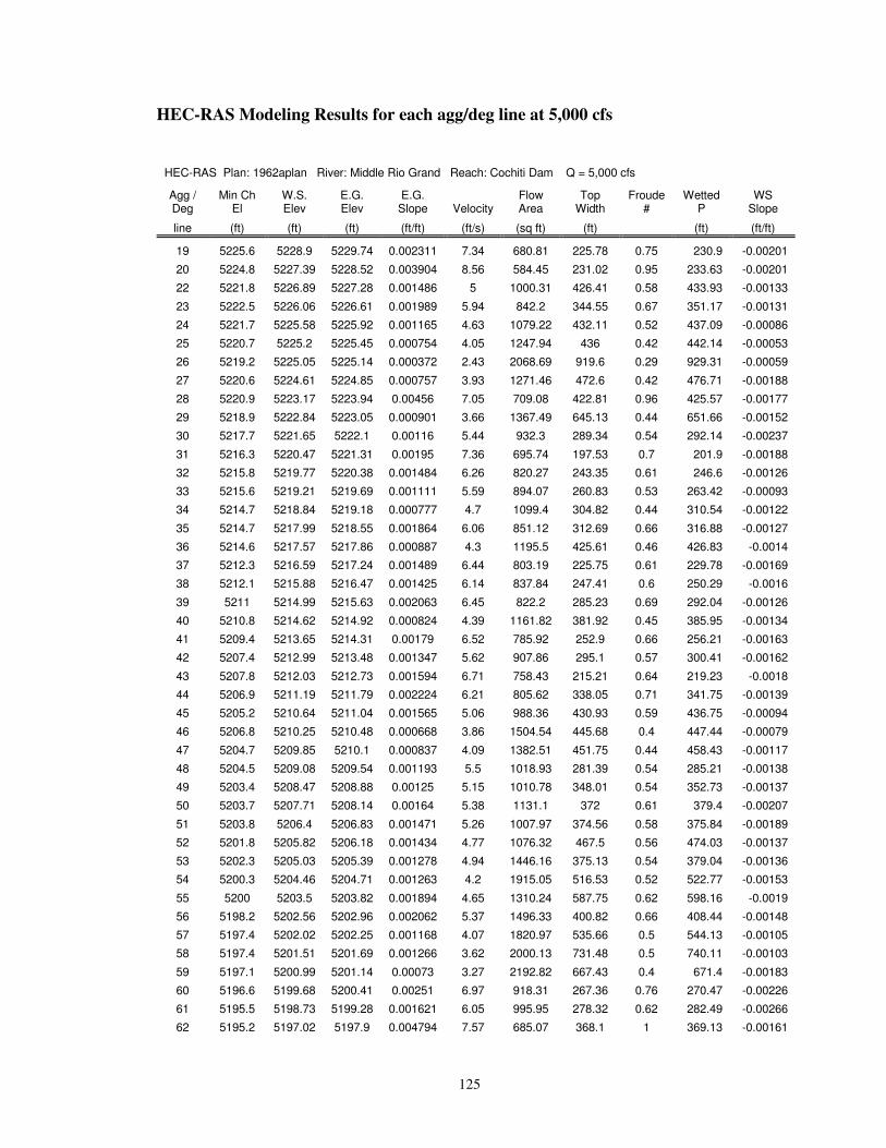
125
HEC-RAS Modeling Results for each agg/deg line at 5,000 cfs
HEC-RAS Plan: 1962aplan River: Middle Rio Grand Reach: Cochiti Dam Q = 5,000 cfs
Agg / Deg
Min Ch El
W.S. Elev
E.G. Elev
E.G. Slope Velocity
Flow Area
Top Width
Froude #
Wetted P
WS Slope
line (ft) (ft) (ft) (ft/ft) (ft/s) (sq ft) (ft) (ft) (ft/ft)
19 5225.6 5228.9 5229.74 0.002311 7.34 680.81 225.78 0.75 230.9 -0.00201
20 5224.8 5227.39 5228.52 0.003904 8.56 584.45 231.02 0.95 233.63 -0.00201
22 5221.8 5226.89 5227.28 0.001486 5 1000.31 426.41 0.58 433.93 -0.00133
23 5222.5 5226.06 5226.61 0.001989 5.94 842.2 344.55 0.67 351.17 -0.00131
24 5221.7 5225.58 5225.92 0.001165 4.63 1079.22 432.11 0.52 437.09 -0.00086
25 5220.7 5225.2 5225.45 0.000754 4.05 1247.94 436 0.42 442.14 -0.00053
26 5219.2 5225.05 5225.14 0.000372 2.43 2068.69 919.6 0.29 929.31 -0.00059
27 5220.6 5224.61 5224.85 0.000757 3.93 1271.46 472.6 0.42 476.71 -0.00188
28 5220.9 5223.17 5223.94 0.00456 7.05 709.08 422.81 0.96 425.57 -0.00177
29 5218.9 5222.84 5223.05 0.000901 3.66 1367.49 645.13 0.44 651.66 -0.00152
30 5217.7 5221.65 5222.1 0.00116 5.44 932.3 289.34 0.54 292.14 -0.00237
31 5216.3 5220.47 5221.31 0.00195 7.36 695.74 197.53 0.7 201.9 -0.00188
32 5215.8 5219.77 5220.38 0.001484 6.26 820.27 243.35 0.61 246.6 -0.00126
33 5215.6 5219.21 5219.69 0.001111 5.59 894.07 260.83 0.53 263.42 -0.00093
34 5214.7 5218.84 5219.18 0.000777 4.7 1099.4 304.82 0.44 310.54 -0.00122
35 5214.7 5217.99 5218.55 0.001864 6.06 851.12 312.69 0.66 316.88 -0.00127
36 5214.6 5217.57 5217.86 0.000887 4.3 1195.5 425.61 0.46 426.83 -0.0014
37 5212.3 5216.59 5217.24 0.001489 6.44 803.19 225.75 0.61 229.78 -0.00169
38 5212.1 5215.88 5216.47 0.001425 6.14 837.84 247.41 0.6 250.29 -0.0016
39 5211 5214.99 5215.63 0.002063 6.45 822.2 285.23 0.69 292.04 -0.00126
40 5210.8 5214.62 5214.92 0.000824 4.39 1161.82 381.92 0.45 385.95 -0.00134
41 5209.4 5213.65 5214.31 0.00179 6.52 785.92 252.9 0.66 256.21 -0.00163
42 5207.4 5212.99 5213.48 0.001347 5.62 907.86 295.1 0.57 300.41 -0.00162
43 5207.8 5212.03 5212.73 0.001594 6.71 758.43 215.21 0.64 219.23 -0.0018
44 5206.9 5211.19 5211.79 0.002224 6.21 805.62 338.05 0.71 341.75 -0.00139
45 5205.2 5210.64 5211.04 0.001565 5.06 988.36 430.93 0.59 436.75 -0.00094
46 5206.8 5210.25 5210.48 0.000668 3.86 1504.54 445.68 0.4 447.44 -0.00079
47 5204.7 5209.85 5210.1 0.000837 4.09 1382.51 451.75 0.44 458.43 -0.00117
48 5204.5 5209.08 5209.54 0.001193 5.5 1018.93 281.39 0.54 285.21 -0.00138
49 5203.4 5208.47 5208.88 0.00125 5.15 1010.78 348.01 0.54 352.73 -0.00137
50 5203.7 5207.71 5208.14 0.00164 5.38 1131.1 372 0.61 379.4 -0.00207
51 5203.8 5206.4 5206.83 0.001471 5.26 1007.97 374.56 0.58 375.84 -0.00189
52 5201.8 5205.82 5206.18 0.001434 4.77 1076.32 467.5 0.56 474.03 -0.00137
53 5202.3 5205.03 5205.39 0.001278 4.94 1446.16 375.13 0.54 379.04 -0.00136
54 5200.3 5204.46 5204.71 0.001263 4.2 1915.05 516.53 0.52 522.77 -0.00153
55 5200 5203.5 5203.82 0.001894 4.65 1310.24 587.75 0.62 598.16 -0.0019
56 5198.2 5202.56 5202.96 0.002062 5.37 1496.33 400.82 0.66 408.44 -0.00148
57 5197.4 5202.02 5202.25 0.001168 4.07 1820.97 535.66 0.5 544.13 -0.00105
58 5197.4 5201.51 5201.69 0.001266 3.62 2000.13 731.48 0.5 740.11 -0.00103
59 5197.1 5200.99 5201.14 0.00073 3.27 2192.82 667.43 0.4 671.4 -0.00183
60 5196.6 5199.68 5200.41 0.00251 6.97 918.31 267.36 0.76 270.47 -0.00226
61 5195.5 5198.73 5199.28 0.001621 6.05 995.95 278.32 0.62 282.49 -0.00266
62 5195.2 5197.02 5197.9 0.004794 7.57 685.07 368.1 1 369.13 -0.00161
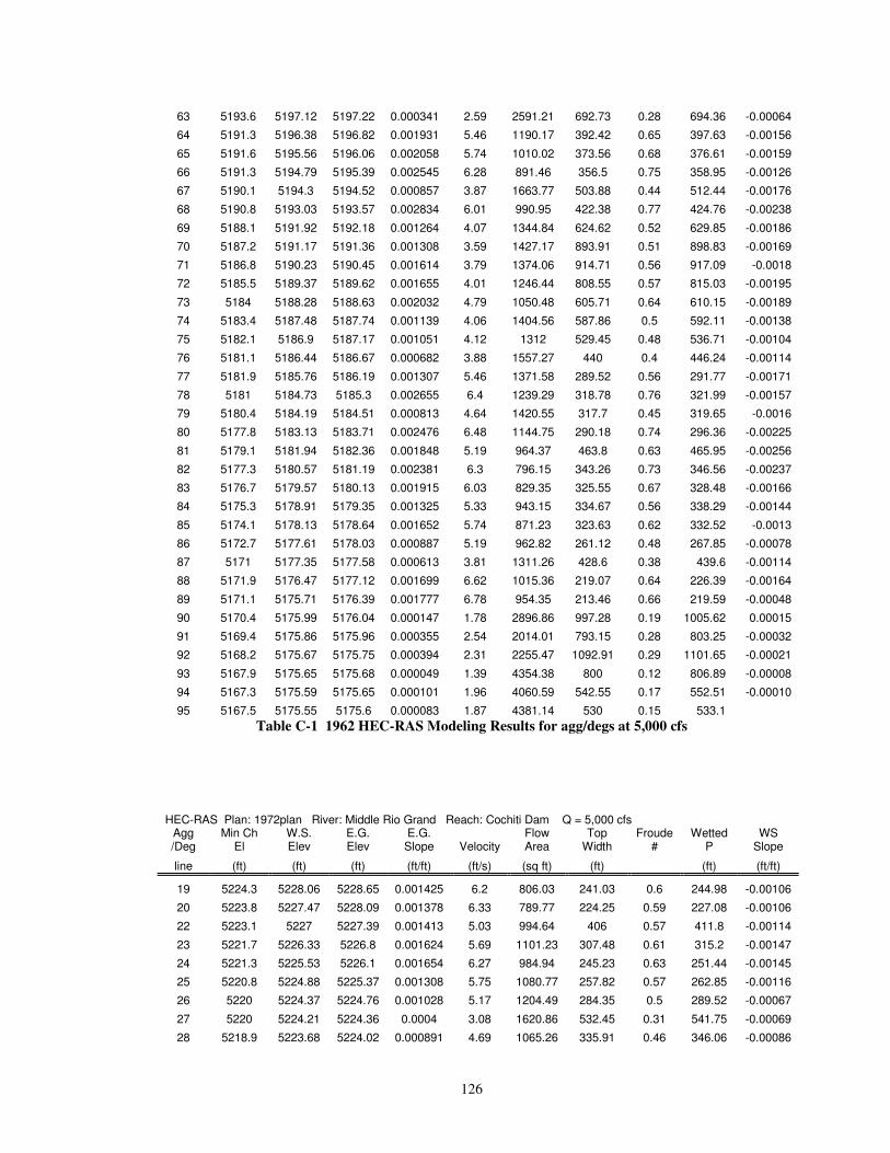
126
63 5193.6 5197.12 5197.22 0.000341 2.59 2591.21 692.73 0.28 694.36 -0.00064
64 5191.3 5196.38 5196.82 0.001931 5.46 1190.17 392.42 0.65 397.63 -0.00156
65 5191.6 5195.56 5196.06 0.002058 5.74 1010.02 373.56 0.68 376.61 -0.00159
66 5191.3 5194.79 5195.39 0.002545 6.28 891.46 356.5 0.75 358.95 -0.00126
67 5190.1 5194.3 5194.52 0.000857 3.87 1663.77 503.88 0.44 512.44 -0.00176
68 5190.8 5193.03 5193.57 0.002834 6.01 990.95 422.38 0.77 424.76 -0.00238
69 5188.1 5191.92 5192.18 0.001264 4.07 1344.84 624.62 0.52 629.85 -0.00186
70 5187.2 5191.17 5191.36 0.001308 3.59 1427.17 893.91 0.51 898.83 -0.00169
71 5186.8 5190.23 5190.45 0.001614 3.79 1374.06 914.71 0.56 917.09 -0.0018
72 5185.5 5189.37 5189.62 0.001655 4.01 1246.44 808.55 0.57 815.03 -0.00195
73 5184 5188.28 5188.63 0.002032 4.79 1050.48 605.71 0.64 610.15 -0.00189
74 5183.4 5187.48 5187.74 0.001139 4.06 1404.56 587.86 0.5 592.11 -0.00138
75 5182.1 5186.9 5187.17 0.001051 4.12 1312 529.45 0.48 536.71 -0.00104
76 5181.1 5186.44 5186.67 0.000682 3.88 1557.27 440 0.4 446.24 -0.00114
77 5181.9 5185.76 5186.19 0.001307 5.46 1371.58 289.52 0.56 291.77 -0.00171
78 5181 5184.73 5185.3 0.002655 6.4 1239.29 318.78 0.76 321.99 -0.00157
79 5180.4 5184.19 5184.51 0.000813 4.64 1420.55 317.7 0.45 319.65 -0.0016
80 5177.8 5183.13 5183.71 0.002476 6.48 1144.75 290.18 0.74 296.36 -0.00225
81 5179.1 5181.94 5182.36 0.001848 5.19 964.37 463.8 0.63 465.95 -0.00256
82 5177.3 5180.57 5181.19 0.002381 6.3 796.15 343.26 0.73 346.56 -0.00237
83 5176.7 5179.57 5180.13 0.001915 6.03 829.35 325.55 0.67 328.48 -0.00166
84 5175.3 5178.91 5179.35 0.001325 5.33 943.15 334.67 0.56 338.29 -0.00144
85 5174.1 5178.13 5178.64 0.001652 5.74 871.23 323.63 0.62 332.52 -0.0013
86 5172.7 5177.61 5178.03 0.000887 5.19 962.82 261.12 0.48 267.85 -0.00078
87 5171 5177.35 5177.58 0.000613 3.81 1311.26 428.6 0.38 439.6 -0.00114
88 5171.9 5176.47 5177.12 0.001699 6.62 1015.36 219.07 0.64 226.39 -0.00164
89 5171.1 5175.71 5176.39 0.001777 6.78 954.35 213.46 0.66 219.59 -0.00048
90 5170.4 5175.99 5176.04 0.000147 1.78 2896.86 997.28 0.19 1005.62 0.00015
91 5169.4 5175.86 5175.96 0.000355 2.54 2014.01 793.15 0.28 803.25 -0.00032
92 5168.2 5175.67 5175.75 0.000394 2.31 2255.47 1092.91 0.29 1101.65 -0.00021
93 5167.9 5175.65 5175.68 0.000049 1.39 4354.38 800 0.12 806.89 -0.00008
94 5167.3 5175.59 5175.65 0.000101 1.96 4060.59 542.55 0.17 552.51 -0.00010
95 5167.5 5175.55 5175.6 0.000083 1.87 4381.14 530 0.15 533.1 Table C-1 1962 HEC-RAS Modeling Results for agg/degs at 5,000 cfs
HEC-RAS Plan: 1972plan River: Middle Rio Grand Reach: Cochiti Dam Q = 5,000 cfs Agg /Deg
Min Ch El
W.S. Elev
E.G. Elev
E.G. Slope Velocity
Flow Area
Top Width
Froude #
Wetted P
WS Slope
line (ft) (ft) (ft) (ft/ft) (ft/s) (sq ft) (ft) (ft) (ft/ft)
19 5224.3 5228.06 5228.65 0.001425 6.2 806.03 241.03 0.6 244.98 -0.00106
20 5223.8 5227.47 5228.09 0.001378 6.33 789.77 224.25 0.59 227.08 -0.00106
22 5223.1 5227 5227.39 0.001413 5.03 994.64 406 0.57 411.8 -0.00114
23 5221.7 5226.33 5226.8 0.001624 5.69 1101.23 307.48 0.61 315.2 -0.00147
24 5221.3 5225.53 5226.1 0.001654 6.27 984.94 245.23 0.63 251.44 -0.00145
25 5220.8 5224.88 5225.37 0.001308 5.75 1080.77 257.82 0.57 262.85 -0.00116
26 5220 5224.37 5224.76 0.001028 5.17 1204.49 284.35 0.5 289.52 -0.00067
27 5220 5224.21 5224.36 0.0004 3.08 1620.86 532.45 0.31 541.75 -0.00069
28 5218.9 5223.68 5224.02 0.000891 4.69 1065.26 335.91 0.46 346.06 -0.00086
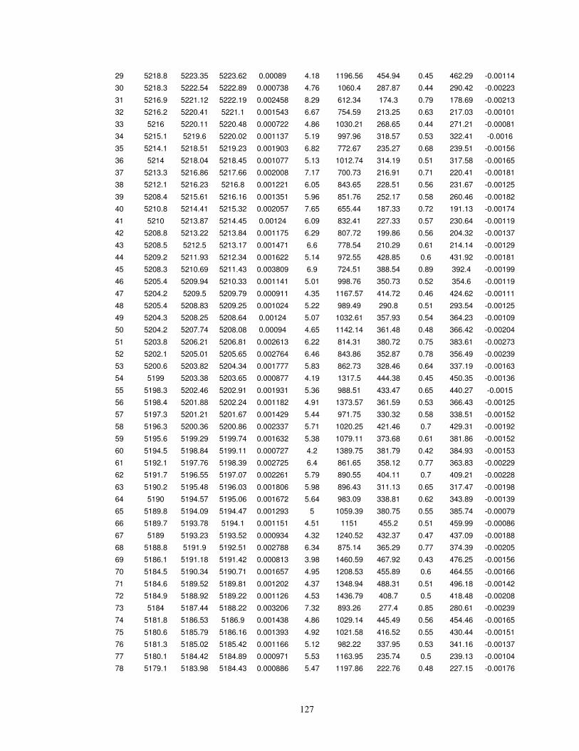
127
29 5218.8 5223.35 5223.62 0.00089 4.18 1196.56 454.94 0.45 462.29 -0.00114
30 5218.3 5222.54 5222.89 0.000738 4.76 1060.4 287.87 0.44 290.42 -0.00223
31 5216.9 5221.12 5222.19 0.002458 8.29 612.34 174.3 0.79 178.69 -0.00213
32 5216.2 5220.41 5221.1 0.001543 6.67 754.59 213.25 0.63 217.03 -0.00101
33 5216 5220.11 5220.48 0.000722 4.86 1030.21 268.65 0.44 271.21 -0.00081
34 5215.1 5219.6 5220.02 0.001137 5.19 997.96 318.57 0.53 322.41 -0.0016
35 5214.1 5218.51 5219.23 0.001903 6.82 772.67 235.27 0.68 239.51 -0.00156
36 5214 5218.04 5218.45 0.001077 5.13 1012.74 314.19 0.51 317.58 -0.00165
37 5213.3 5216.86 5217.66 0.002008 7.17 700.73 216.91 0.71 220.41 -0.00181
38 5212.1 5216.23 5216.8 0.001221 6.05 843.65 228.51 0.56 231.67 -0.00125
39 5208.4 5215.61 5216.16 0.001351 5.96 851.76 252.17 0.58 260.46 -0.00182
40 5210.8 5214.41 5215.32 0.002057 7.65 655.44 187.33 0.72 191.13 -0.00174
41 5210 5213.87 5214.45 0.00124 6.09 832.41 227.33 0.57 230.64 -0.00119
42 5208.8 5213.22 5213.84 0.001175 6.29 807.72 199.86 0.56 204.32 -0.00137
43 5208.5 5212.5 5213.17 0.001471 6.6 778.54 210.29 0.61 214.14 -0.00129
44 5209.2 5211.93 5212.34 0.001622 5.14 972.55 428.85 0.6 431.92 -0.00181
45 5208.3 5210.69 5211.43 0.003809 6.9 724.51 388.54 0.89 392.4 -0.00199
46 5205.4 5209.94 5210.33 0.001141 5.01 998.76 350.73 0.52 354.6 -0.00119
47 5204.2 5209.5 5209.79 0.000911 4.35 1167.57 414.72 0.46 424.62 -0.00111
48 5205.4 5208.83 5209.25 0.001024 5.22 989.49 290.8 0.51 293.54 -0.00125
49 5204.3 5208.25 5208.64 0.00124 5.07 1032.61 357.93 0.54 364.23 -0.00109
50 5204.2 5207.74 5208.08 0.00094 4.65 1142.14 361.48 0.48 366.42 -0.00204
51 5203.8 5206.21 5206.81 0.002613 6.22 814.31 380.72 0.75 383.61 -0.00273
52 5202.1 5205.01 5205.65 0.002764 6.46 843.86 352.87 0.78 356.49 -0.00239
53 5200.6 5203.82 5204.34 0.001777 5.83 862.73 328.46 0.64 337.19 -0.00163
54 5199 5203.38 5203.65 0.000877 4.19 1317.5 444.38 0.45 450.35 -0.00136
55 5198.3 5202.46 5202.91 0.001931 5.36 988.51 433.47 0.65 440.27 -0.0015
56 5198.4 5201.88 5202.24 0.001182 4.91 1373.57 361.59 0.53 366.43 -0.00125
57 5197.3 5201.21 5201.67 0.001429 5.44 971.75 330.32 0.58 338.51 -0.00152
58 5196.3 5200.36 5200.86 0.002337 5.71 1020.25 421.46 0.7 429.31 -0.00192
59 5195.6 5199.29 5199.74 0.001632 5.38 1079.11 373.68 0.61 381.86 -0.00152
60 5194.5 5198.84 5199.11 0.000727 4.2 1389.75 381.79 0.42 384.93 -0.00153
61 5192.1 5197.76 5198.39 0.002725 6.4 861.65 358.12 0.77 363.83 -0.00229
62 5191.7 5196.55 5197.07 0.002261 5.79 890.55 404.11 0.7 409.21 -0.00228
63 5190.2 5195.48 5196.03 0.001806 5.98 896.43 311.13 0.65 317.47 -0.00198
64 5190 5194.57 5195.06 0.001672 5.64 983.09 338.81 0.62 343.89 -0.00139
65 5189.8 5194.09 5194.47 0.001293 5 1059.39 380.75 0.55 385.74 -0.00079
66 5189.7 5193.78 5194.1 0.001151 4.51 1151 455.2 0.51 459.99 -0.00086
67 5189 5193.23 5193.52 0.000934 4.32 1240.52 432.37 0.47 437.09 -0.00188
68 5188.8 5191.9 5192.51 0.002788 6.34 875.14 365.29 0.77 374.39 -0.00205
69 5186.1 5191.18 5191.42 0.000813 3.98 1460.59 467.92 0.43 476.25 -0.00156
70 5184.5 5190.34 5190.71 0.001657 4.95 1208.53 455.89 0.6 464.55 -0.00166
71 5184.6 5189.52 5189.81 0.001202 4.37 1348.94 488.31 0.51 496.18 -0.00142
72 5184.9 5188.92 5189.22 0.001126 4.53 1436.79 408.7 0.5 418.48 -0.00208
73 5184 5187.44 5188.22 0.003206 7.32 893.26 277.4 0.85 280.61 -0.00239
74 5181.8 5186.53 5186.9 0.001438 4.86 1029.14 445.49 0.56 454.46 -0.00165
75 5180.6 5185.79 5186.16 0.001393 4.92 1021.58 416.52 0.55 430.44 -0.00151
76 5181.3 5185.02 5185.42 0.001166 5.12 982.22 337.95 0.53 341.16 -0.00137
77 5180.1 5184.42 5184.89 0.000971 5.53 1163.95 235.74 0.5 239.13 -0.00104
78 5179.1 5183.98 5184.43 0.000886 5.47 1197.86 222.76 0.48 227.15 -0.00176
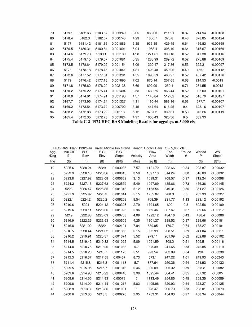
128
79 5179.1 5182.66 5183.57 0.003249 8.05 866.03 211.21 0.87 214.94 -0.00168
80 5178.4 5182.3 5182.57 0.000743 4.23 1356.7 375.8 0.43 378.85 -0.00124
81 5177 5181.42 5181.86 0.001886 5.35 933.85 429.45 0.64 436.83 -0.00199
82 5176.5 5180.31 5180.84 0.001801 5.94 1063.4 306.49 0.64 315.67 -0.00169
83 5174.6 5179.73 5180.1 0.001139 4.98 1271.61 339.18 0.52 347.38 -0.00116
84 5175.4 5179.15 5179.57 0.001081 5.35 1288.99 269.72 0.52 275.88 -0.00109
85 5173.5 5178.64 5179.02 0.001154 5.09 1320.47 317.36 0.53 322.31 -0.00097
86 5173 5178.18 5178.45 0.001041 4.31 1428.48 450.26 0.49 455.1 -0.00112
87 5172.6 5177.52 5177.84 0.001201 4.55 1098.59 460.27 0.52 467.42 -0.00176
88 5172 5176.42 5177.16 0.001895 7.02 870.14 207.65 0.68 214.53 -0.0019
89 5171.8 5175.62 5176.29 0.002136 6.69 892.99 259.1 0.71 264.55 -0.0012
90 5170.2 5175.22 5175.41 0.001404 3.53 1460.75 966.44 0.52 985.03 -0.00101
91 5170.8 5174.61 5174.91 0.001198 4.37 1145.04 512.62 0.52 516.79 -0.00127
92 5167.7 5173.95 5174.24 0.001327 4.31 1160.44 566.16 0.53 577.7 -0.00107
93 5169.2 5173.54 5173.72 0.000702 3.45 1447.64 616.25 0.4 623.16 -0.00107
94 5168.2 5172.88 5173.29 0.00118 5.12 976.02 332.61 0.53 343.26 -0.00119
95 5165.4 5172.35 5172.73 0.001024 4.97 1005.43 325.36 0.5 332.33 Table C-2 1972 HEC-RAS Modeling Results for agg/degs at 5,000 cfs
HEC-RAS Plan: 1992plan River: Middle Rio Grand Reach: Cochiti Dam Q = 5,000 cfs Agg /Deg
Min Ch El
W.S. Elev
E.G. Elev
E.G. Slope Velocity
Flow Area
Top Width
Froude #
Wetted P
WS Slope
line (ft) (ft) (ft) (ft/ft) (ft/s) (sq ft) (ft) (ft) (ft/ft)
19 5225.6 5228.24 5229 0.003036 7.57 1121.72 222.66 0.84 223.87 -0.00032
20 5223.9 5228.16 5228.36 0.000615 3.58 1397.13 514.24 0.38 516.03 -0.00032
22 5223.8 5227.92 5228.08 0.000602 3.13 1599.31 708.57 0.37 712.24 -0.00098
23 5224.2 5227.18 5227.63 0.002579 5.49 1097.09 485.66 0.73 486.36 -0.00145
24 5223 5226.47 5226.85 0.001313 5.12 1163.54 349.31 0.56 351.27 -0.00126
25 5221.9 5225.92 5226.3 0.001014 5.15 1255.87 280.3 0.5 282.93 -0.00227
26 5222.1 5224.2 5225.2 0.006258 8.54 768.39 291.77 1.13 293.12 -0.00192
27 5219.6 5224 5224.12 0.000395 2.79 1794.65 690 0.3 692.56 -0.00109
28 5219.6 5223.11 5223.66 0.001923 5.96 839.46 337.67 0.67 339.66 -0.00117
29 5219 5222.83 5223.09 0.000768 4.09 1222.12 434.16 0.43 436.4 -0.00086
30 5216.9 5222.25 5222.53 0.000505 4.25 1201.27 288.52 0.37 289.66 -0.00181
31 5216.8 5221.02 5222 0.002121 7.94 630.95 176.7 0.74 178.27 -0.00181
32 5216.5 5220.44 5221.02 0.001358 6.15 822.99 238.51 0.59 241.04 -0.00111
33 5216.2 5219.91 5220.37 0.001074 5.52 979.11 261.09 0.52 262.88 -0.00102
34 5214.5 5219.42 5219.82 0.001025 5.09 1091.59 308.2 0.51 309.51 -0.00116
35 5214.8 5218.75 5219.26 0.001068 5.7 908.39 241.65 0.53 242.85 -0.00119
36 5214.5 5218.23 5218.7 0.001173 5.51 923.54 282.89 0.54 284 -0.00238
37 5212.3 5216.37 5217.55 0.00457 8.73 573.1 247.22 1.01 249.93 -0.00243
38 5211.4 5215.8 5216.3 0.001113 5.7 877.64 250.36 0.54 251.93 -0.00132
39 5209.5 5215.05 5215.7 0.001316 6.46 800.09 205.32 0.59 208.2 -0.00082
40 5209.6 5214.98 5215.22 0.000446 3.98 1395.44 304.41 0.35 307.32 -0.0005
41 5209.6 5214.55 5214.93 0.00076 5 1113.49 254.85 0.45 258.35 -0.00089
42 5209.8 5214.09 5214.44 0.001217 5.03 1405.98 320.93 0.54 323.27 -0.00125
43 5208.9 5213.3 5213.86 0.001031 6 898.47 206.79 0.53 208.01 -0.00073
44 5208.6 5213.36 5213.5 0.000276 2.95 1753.31 454.83 0.27 458.34 -0.00044
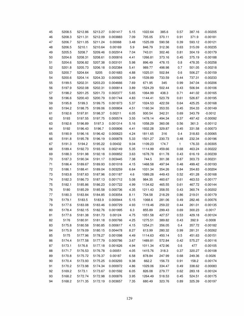
129
45 5208.5 5212.86 5213.27 0.001417 5.15 1022.64 385.6 0.57 387.16 -0.00205
46 5208.3 5211.31 5212.09 0.003883 7.09 705.05 370.11 0.91 371.9 -0.00181
47 5206.7 5211.05 5211.24 0.00068 3.48 1525.09 590.58 0.39 593.12 -0.00121
48 5206.5 5210.1 5210.64 0.00169 5.9 846.79 312.36 0.63 315.09 -0.00235
49 5205.5 5208.7 5209.46 0.002914 7.04 743.01 302.46 0.81 304.19 -0.00179
50 5204.6 5208.31 5208.61 0.000816 4.41 1266.81 373.16 0.45 375.19 -0.00188
51 5204.6 5206.82 5207.38 0.003101 5.98 896.49 478.15 0.8 478.35 -0.00258
52 5201.8 5205.73 5206.18 0.002384 5.41 989.77 498.98 0.7 501.05 -0.00218
53 5200.7 5204.64 5205 0.001683 4.88 1025.01 502.84 0.6 506.27 -0.00159
54 5200.6 5204.14 5204.33 0.000925 3.49 1539.89 733.59 0.44 737.31 -0.00233
55 5199.5 5202.31 5203.23 0.004666 7.69 671.95 345 0.99 347.04 -0.00206
56 5197.9 5202.08 5202.31 0.000814 3.89 1524.29 502.44 0.43 506.94 -0.00106
57 5198.2 5201.25 5201.73 0.002377 5.65 1064.99 438.3 0.71 441.02 -0.00165
58 5196.6 5200.43 5200.79 0.001744 4.83 1144.41 523.79 0.61 526.87 -0.00195
59 5195.8 5199.3 5199.75 0.001873 5.37 1024.53 422.59 0.64 425.25 -0.00168
60 5194.2 5198.75 5199.06 0.000804 4.51 1160.34 353.55 0.45 354.33 -0.00149
61 5192.6 5197.81 5198.37 0.00211 6.05 930.54 342.31 0.69 343.79 -0.0012
62 5193 5197.55 5197.75 0.000574 3.55 1478.14 494.34 0.37 497.42 -0.00092
63 5192.6 5196.89 5197.3 0.001314 5.16 1058.29 360.08 0.56 361.3 -0.00112
64 5192 5196.43 5196.7 0.000806 4.41 1932.28 329.87 0.45 331.58 -0.00073
65 5190.9 5196.16 5196.42 0.000623 4.24 1811.65 316 0.4 318.83 -0.00065
66 5191.8 5195.78 5196.19 0.000878 5.33 1501.27 230.73 0.48 232.34 -0.00196
67 5191.3 5194.2 5195.22 0.00432 9.04 1109.23 174.7 1 176.33 -0.00305
68 5189.4 5192.73 5193.16 0.002149 5.35 1114.99 459.66 0.68 463.24 -0.00222
69 5188.3 5191.98 5192.18 0.000852 3.63 1678.78 611.78 0.43 616.19 -0.00239
70 5187.3 5190.34 5191.17 0.003445 7.38 744.5 301.38 0.87 303.73 -0.00231
71 5186.4 5189.67 5189.93 0.001018 4.15 1468.58 497.94 0.48 499.42 -0.00193
72 5186.1 5188.41 5189.04 0.003259 6.64 1031.34 354.26 0.84 354.83 -0.00204
73 5183.8 5187.63 5187.96 0.001187 4.6 1089.28 449.43 0.52 451.28 -0.00168
74 5182.3 5186.73 5187.13 0.001712 5.08 984.35 460.67 0.61 463.53 -0.00177
75 5182.1 5185.86 5186.23 0.001722 4.99 1134.62 465.55 0.61 467.72 -0.00144
76 5180 5185.29 5185.58 0.000736 4.35 1211.43 358.55 0.43 360.74 -0.00202
77 5180.3 5183.84 5184.85 0.003054 8.11 704.58 218.29 0.86 219.01 -0.00179
78 5179.1 5183.5 5183.9 0.000944 5.15 1068.6 281.06 0.49 282.46 -0.00076
79 5177.6 5183.08 5183.46 0.000729 4.93 1119.46 259.22 0.44 261.01 -0.00135
80 5178.4 5182.15 5182.76 0.001995 6.3 855.89 299.43 0.69 300.23 -0.0017
81 5177.6 5181.38 5181.73 0.00124 4.75 1051.58 427.57 0.53 429.18 -0.00124
82 5176 5180.91 5181.18 0.000766 4.25 1275.51 389.82 0.43 392.9 -0.0008
83 5175.8 5180.58 5180.85 0.000617 4.15 1254.21 356.05 0.4 357.72 -0.00182
84 5175.9 5179.09 5180.15 0.004478 8.27 613.99 280.32 0.99 281.31 -0.00262
85 5175 5177.96 5178.27 0.001098 4.49 1114.63 450.14 0.5 451.63 -0.00151
86 5174.4 5177.58 5177.79 0.000786 3.67 1489.81 572.84 0.42 575.27 -0.00116
87 5173.1 5176.8 5177.18 0.001626 4.94 1011.34 472.96 0.6 477 -0.00105
88 5171.7 5176.53 5176.78 0.00051 4.05 1415.76 318.3 0.37 320.27 -0.00108
89 5170.8 5175.72 5176.37 0.00187 6.58 878.84 247.99 0.68 249.36 -0.0026
90 5170.4 5173.93 5175.25 0.003293 9.38 662.2 156.73 0.91 158.2 -0.00174
91 5170.2 5173.98 5174.34 0.000972 4.86 1029.06 334.47 0.49 338.62 -0.00083
92 5169.2 5173.1 5173.67 0.001592 6.05 826.08 279.77 0.62 283.18 -0.00124
93 5168.2 5172.74 5172.98 0.000876 3.95 1264.49 518.53 0.45 524.51 -0.00175
94 5168.2 5171.35 5172.19 0.003657 7.35 680.49 323.76 0.89 325.39 -0.00197
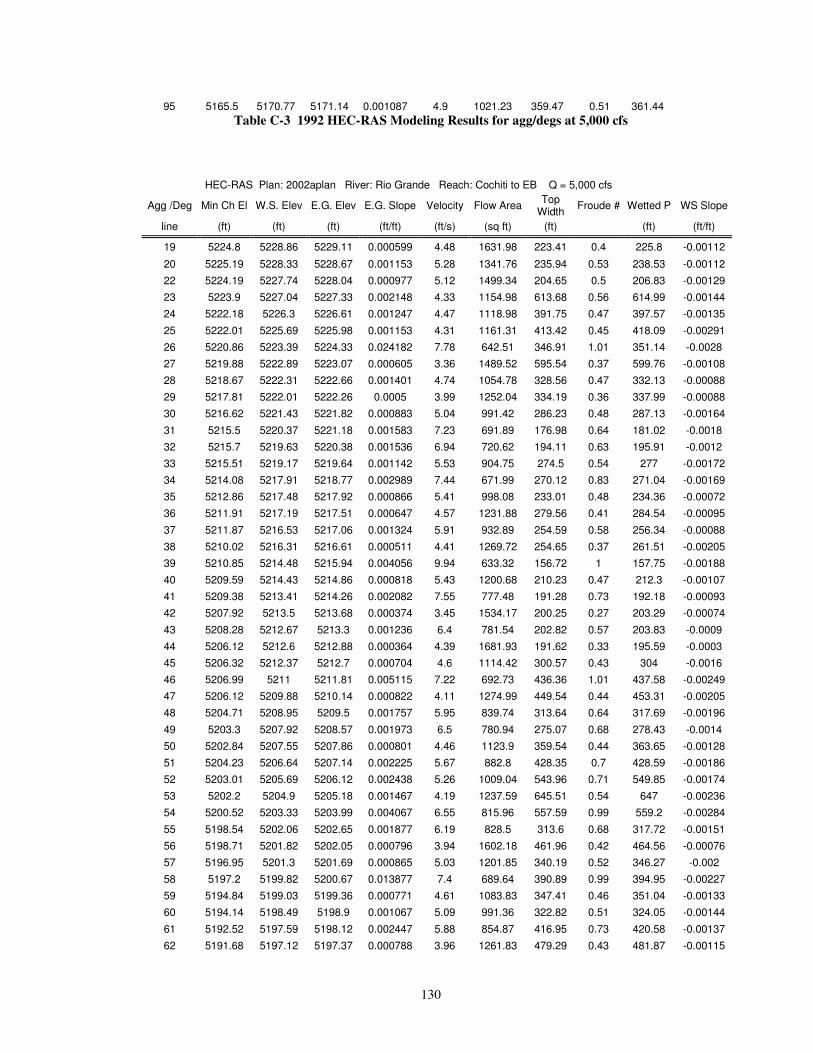
130
95 5165.5 5170.77 5171.14 0.001087 4.9 1021.23 359.47 0.51 361.44 Table C-3 1992 HEC-RAS Modeling Results for agg/degs at 5,000 cfs
HEC-RAS Plan: 2002aplan River: Rio Grande Reach: Cochiti to EB Q = 5,000 cfs
Agg /Deg Min Ch El W.S. Elev E.G. Elev E.G. Slope Velocity Flow Area Top Width Froude # Wetted P WS Slope
line (ft) (ft) (ft) (ft/ft) (ft/s) (sq ft) (ft) (ft) (ft/ft)
19 5224.8 5228.86 5229.11 0.000599 4.48 1631.98 223.41 0.4 225.8 -0.00112
20 5225.19 5228.33 5228.67 0.001153 5.28 1341.76 235.94 0.53 238.53 -0.00112
22 5224.19 5227.74 5228.04 0.000977 5.12 1499.34 204.65 0.5 206.83 -0.00129
23 5223.9 5227.04 5227.33 0.002148 4.33 1154.98 613.68 0.56 614.99 -0.00144
24 5222.18 5226.3 5226.61 0.001247 4.47 1118.98 391.75 0.47 397.57 -0.00135
25 5222.01 5225.69 5225.98 0.001153 4.31 1161.31 413.42 0.45 418.09 -0.00291
26 5220.86 5223.39 5224.33 0.024182 7.78 642.51 346.91 1.01 351.14 -0.0028
27 5219.88 5222.89 5223.07 0.000605 3.36 1489.52 595.54 0.37 599.76 -0.00108
28 5218.67 5222.31 5222.66 0.001401 4.74 1054.78 328.56 0.47 332.13 -0.00088
29 5217.81 5222.01 5222.26 0.0005 3.99 1252.04 334.19 0.36 337.99 -0.00088
30 5216.62 5221.43 5221.82 0.000883 5.04 991.42 286.23 0.48 287.13 -0.00164
31 5215.5 5220.37 5221.18 0.001583 7.23 691.89 176.98 0.64 181.02 -0.0018
32 5215.7 5219.63 5220.38 0.001536 6.94 720.62 194.11 0.63 195.91 -0.0012
33 5215.51 5219.17 5219.64 0.001142 5.53 904.75 274.5 0.54 277 -0.00172
34 5214.08 5217.91 5218.77 0.002989 7.44 671.99 270.12 0.83 271.04 -0.00169
35 5212.86 5217.48 5217.92 0.000866 5.41 998.08 233.01 0.48 234.36 -0.00072
36 5211.91 5217.19 5217.51 0.000647 4.57 1231.88 279.56 0.41 284.54 -0.00095
37 5211.87 5216.53 5217.06 0.001324 5.91 932.89 254.59 0.58 256.34 -0.00088
38 5210.02 5216.31 5216.61 0.000511 4.41 1269.72 254.65 0.37 261.51 -0.00205
39 5210.85 5214.48 5215.94 0.004056 9.94 633.32 156.72 1 157.75 -0.00188
40 5209.59 5214.43 5214.86 0.000818 5.43 1200.68 210.23 0.47 212.3 -0.00107
41 5209.38 5213.41 5214.26 0.002082 7.55 777.48 191.28 0.73 192.18 -0.00093
42 5207.92 5213.5 5213.68 0.000374 3.45 1534.17 200.25 0.27 203.29 -0.00074
43 5208.28 5212.67 5213.3 0.001236 6.4 781.54 202.82 0.57 203.83 -0.0009
44 5206.12 5212.6 5212.88 0.000364 4.39 1681.93 191.62 0.33 195.59 -0.0003
45 5206.32 5212.37 5212.7 0.000704 4.6 1114.42 300.57 0.43 304 -0.0016
46 5206.99 5211 5211.81 0.005115 7.22 692.73 436.36 1.01 437.58 -0.00249
47 5206.12 5209.88 5210.14 0.000822 4.11 1274.99 449.54 0.44 453.31 -0.00205
48 5204.71 5208.95 5209.5 0.001757 5.95 839.74 313.64 0.64 317.69 -0.00196
49 5203.3 5207.92 5208.57 0.001973 6.5 780.94 275.07 0.68 278.43 -0.0014
50 5202.84 5207.55 5207.86 0.000801 4.46 1123.9 359.54 0.44 363.65 -0.00128
51 5204.23 5206.64 5207.14 0.002225 5.67 882.8 428.35 0.7 428.59 -0.00186
52 5203.01 5205.69 5206.12 0.002438 5.26 1009.04 543.96 0.71 549.85 -0.00174
53 5202.2 5204.9 5205.18 0.001467 4.19 1237.59 645.51 0.54 647 -0.00236
54 5200.52 5203.33 5203.99 0.004067 6.55 815.96 557.59 0.99 559.2 -0.00284
55 5198.54 5202.06 5202.65 0.001877 6.19 828.5 313.6 0.68 317.72 -0.00151
56 5198.71 5201.82 5202.05 0.000796 3.94 1602.18 461.96 0.42 464.56 -0.00076
57 5196.95 5201.3 5201.69 0.000865 5.03 1201.85 340.19 0.52 346.27 -0.002
58 5197.2 5199.82 5200.67 0.013877 7.4 689.64 390.89 0.99 394.95 -0.00227
59 5194.84 5199.03 5199.36 0.000771 4.61 1083.83 347.41 0.46 351.04 -0.00133
60 5194.14 5198.49 5198.9 0.001067 5.09 991.36 322.82 0.51 324.05 -0.00144
61 5192.52 5197.59 5198.12 0.002447 5.88 854.87 416.95 0.73 420.58 -0.00137
62 5191.68 5197.12 5197.37 0.000788 3.96 1261.83 479.29 0.43 481.87 -0.00115
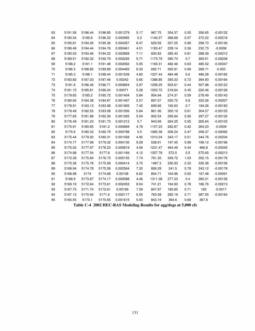
131
63 5191.56 5196.44 5196.85 0.001279 5.17 967.75 354.37 0.55 356.65 -0.00132
64 5190.54 5195.8 5196.22 0.000992 5.2 1140.27 368.69 0.57 372.22 -0.00218
65 5190.81 5194.26 5195.36 0.004357 8.47 629.59 257.25 0.99 258.73 -0.00136
66 5189.49 5194.44 5194.76 0.000461 4.51 1183.47 228.14 0.36 232.73 -0.0008
67 5190.03 5193.46 5194.22 0.002869 7.11 830.83 285.43 0.81 288.39 -0.00212
68 5189.51 5192.32 5192.79 0.002226 5.71 1173.79 390.74 0.7 393.51 -0.00236
69 5188.2 5191.1 5191.48 0.002062 5.05 1183.31 482.46 0.63 485.52 -0.00347
70 5186.3 5188.85 5189.89 0.004483 8.33 692.71 265.91 0.99 268.71 -0.003
71 5185.3 5188.1 5188.44 0.001539 4.82 1227.44 484.48 0.6 486.28 -0.00182
72 5183.82 5187.03 5187.46 0.00242 5.65 1388.85 393.33 0.72 394.93 -0.00164
73 5181.8 5186.46 5186.71 0.000854 3.97 1258.25 503.61 0.44 507.98 -0.00122
74 5181.15 5185.81 5186.24 0.00071 5.28 1053.72 218.64 0.45 220.46 -0.00126
75 5179.65 5185.2 5185.72 0.001404 5.84 954.94 274.31 0.59 278.49 -0.00143
76 5180.65 5184.38 5184.87 0.001497 5.57 897.07 330.72 0.6 332.26 -0.00207
77 5178.91 5183.13 5183.98 0.001905 7.42 699.66 192.63 0.7 194.26 -0.00183
78 5178.49 5182.55 5183.08 0.001556 5.84 861.06 302.19 0.61 304.57 -0.00125
79 5177.65 5181.88 5182.36 0.001265 5.54 902.54 295.64 0.56 297.27 -0.00132
80 5176.49 5181.23 5181.73 0.001212 5.7 943.69 264.25 0.55 265.64 -0.00103
81 5175.91 5180.85 5181.2 0.000669 4.78 1157.23 262.87 0.42 264.23 -0.0009
82 5175.6 5180.33 5180.79 0.000788 5.5 1085.38 206.24 0.47 208.37 -0.00092
83 5175.44 5179.93 5180.31 0.001058 4.95 1010.24 343.17 0.51 344.76 -0.00234
84 5174.77 5177.99 5179.32 0.004135 9.28 538.91 197.45 0.99 199.12 -0.00196
85 5175.02 5177.97 5178.23 0.000819 4.06 1231.47 464.49 0.44 466.8 -0.00045
86 5174.88 5177.54 5177.8 0.001169 4.12 1357.78 572.5 0.5 575.65 -0.00213
87 5172.39 5175.84 5176.73 0.005155 7.74 761.35 349.72 1.03 352.15 -0.00176
88 5170.36 5175.78 5175.99 0.000414 3.75 1487.3 330.93 0.33 335.36 -0.00106
89 5169.94 5174.78 5175.58 0.002564 7.32 806.29 241.5 0.78 243.12 -0.00178
90 5168.98 5174 5174.68 0.00108 6.62 854.71 164.96 0.55 167.48 -0.00091
91 5168.9 5173.87 5174.17 0.000588 4.46 1311.38 277.23 0.4 280.21 -0.00136
92 5169.19 5172.64 5173.61 0.002453 8.04 741.21 184.93 0.78 186.76 -0.00213
93 5167.75 5171.74 5172.61 0.00199 7.59 847.97 180.65 0.71 183 -0.0017
94 5167.13 5170.94 5171.6 0.002117 6.55 763.08 285.19 0.71 287.55 -0.00164
95 5165.55 5170.1 5170.65 0.001615 5.93 843.19 364.6 0.69 367.8
Table C-4 2002 HEC-RAS Modeling Results for agg/degs at 5,000 cfs �
�
�
�
�
�
�
�
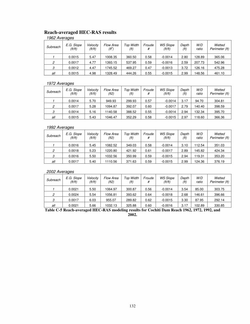
132
Reach-averaged HEC-RAS results 1962 Averages
Subreach E.G. Slope (ft/ft)
Velocity (ft/ft)
Flow Area (ft2)
Top Width (ft)
Froude #
WS Slope (ft/ft)
Depth (ft)
W/D ratio
Wetted Perimeter (ft)
1 0.0015 5.47 1008.35 360.50 0.58 -0.0014 2.80 128.89 365.06
2 0.0017 4.77 1393.15 537.95 0.59 -0.0016 2.59 207.73 542.96
3 0.0012 4.47 1745.52 469.27 0.47 -0.0013 3.72 126.16 475.28
all 0.0015 4.98 1328.49 444.26 0.55 -0.0015 2.99 148.56 461.10
1972 Averages
Subreach E.G. Slope (ft/ft)
Velocity (ft/ft)
Flow Area (ft2)
Top Width (ft)
Froude #
WS Slope (ft/ft)
Depth (ft)
W/D ratio
Wetted Perimeter (ft)
1 0.0014 5.70 949.93 299.93 0.57 -0.0014 3.17 94.70 304.81
2 0.0017 5.28 1094.87 392.07 0.60 -0.0017 2.79 140.40 398.59
3 0.0014 5.16 1140.58 388.52 0.55 -0.0014 2.94 132.34 395.70
all 0.0015 5.43 1046.47 352.29 0.58 -0.0015 2.97 118.60 366.36
1992 Averages
Subreach E.G. Slope (ft/ft)
Velocity (ft/ft)
Flow Area (ft2)
Top Width (ft)
Froude #
WS Slope (ft/ft)
Depth (ft)
W/D ratio
Wetted Perimeter (ft)
1 0.0016 5.45 1082.52 349.03 0.58 -0.0014 3.10 112.54 351.03
2 0.0018 5.23 1220.80 421.92 0.61 -0.0017 2.89 145.82 424.34
3 0.0016 5.50 1032.56 350.99 0.59 -0.0015 2.94 119.31 353.20
all 0.0017 5.40 1110.56 371.63 0.59 -0.0015 2.99 124.36 376.19
2002 Averages
Subreach E.G. Slope (ft/ft)
Velocity (ft/ft)
Flow Area (ft2)
Top Width (ft)
Froude #
WS Slope (ft/ft)
Depth (ft)
W/D ratio
Wetted Perimeter (ft)
1 0.0021 5.50 1064.97 300.87 0.56 -0.0014 3.54 85.00 303.75
2 0.0024 5.54 1056.81 393.62 0.64 -0.0018 2.68 146.61 396.66
3 0.0017 6.03 955.07 289.82 0.62 -0.0015 3.30 87.95 292.14
all 0.0021 5.66 1032.13 325.88 0.60 -0.0016 3.17 102.89 330.85 Table C-5 Reach-averaged HEC-RAS modeling results for Cochiti Dam Reach 1962, 1972, 1992, and
2002. �
�
�
�
�
�
�

133
�
�
�
�
�
�
�
�
�
�
�
A P P E N D I X D – B E D M A T E R I A L P L O T S
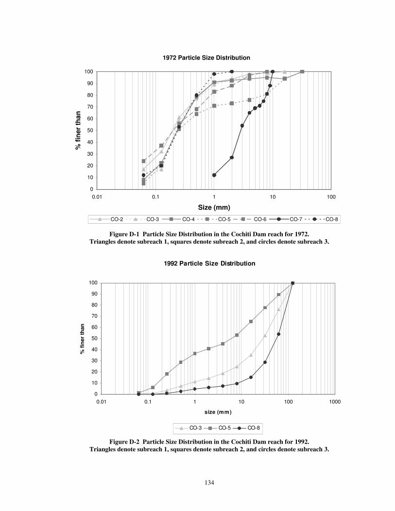
134
1972 Particle Size Distribution
0
10
20
30
40
50
60
70
80
90
100
0.01 0.1 1 10 100
Size (mm)
% fi
ner
than
CO-2 CO-3 CO-4 CO-5 CO-6 CO-7 CO-8
�Figure D-1 Particle Size Distribution in the Cochiti Dam reach for 1972.
Triangles denote subreach 1, squares denote subreach 2, and circles denote subreach 3.
1992 Particle Size Distribution
0
10
20
30
40
50
60
70
80
90
100
0.01 0.1 1 10 100 1000
size (mm)
% fi
ner
than
CO-3 CO-5 CO-8
Figure D-2 Particle Size Distribution in the Cochiti Dam reach for 1992.
Triangles denote subreach 1, squares denote subreach 2, and circles denote subreach 3.
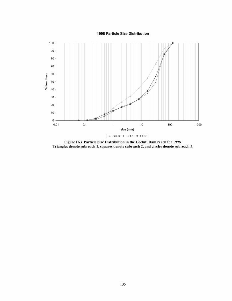
135
1998 Particle Size Distribution
0
10
20
30
40
50
60
70
80
90
100
0.01 0.1 1 10 100 1000
size (mm)
% fi
ner
than
CO-3 CO-5 CO-8 Figure D-3 Particle Size Distribution in the Cochiti Dam reach for 1998.
Triangles denote subreach 1, squares denote subreach 2, and circles denote subreach 3.
136
A P P E N D I X E – S E D I M E N T T R A N S P OR T C A P A C I T Y
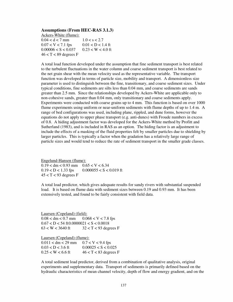
137
Assumptions (From HEC-RAS 3.1.3) Ackers-White (flume): 0.04 < d < 7 mm 1.0 < s < 2.7 0.07 < V < 7.1 fps 0.01 < D < 1.4 ft 0.00006 < S < 0.037 0.23 < W < 4.0 ft 46 < T < 89 degrees F A total load function developed under the assumption that fine sediment transport is best related to the turbulent fluctuations in the water column and coarse sediment transport is best related to the net grain shear with the mean velocity used as the representative variable. The transport function was developed in terms of particle size, mobility and transport. A dimensionless size parameter is used to distinguish between the fine, transitionary, and coarse sediment sizes. Under typical conditions, fine sediments are silts less than 0.04 mm, and coarse sediments are sands greater than 2.5 mm. Since the relationships developed by Ackers-White are applicable only to non-cohesive sands, greater than 0.04 mm, only transitionary and coarse sediments apply. Experiments were conducted with coarse grains up to 4 mm. This function is based on over 1000 flume experiments using uniform or near-uniform sediments with flume depths of up to 1.4 m. A range of bed configurations was used, including plane, rippled, and dune forms, however the equations do not apply to upper phase transport (e.g. anti-dunes) with Froude numbers in excess of 0.8. A hiding adjustment factor was developed for the Ackers-White method by Profitt and Sutherland (1983), and is included in RAS as an option. The hiding factor is an adjustment to include the effects of a masking of the fluid properties felt by smaller particles due to shielding by larger particles. This is typically a factor when the gradation has a relatively large range of particle sizes and would tend to reduce the rate of sediment transport in the smaller grade classes. Engelund-Hansen (flume): 0.19 < dm < 0.93 mm 0.65 < V < 6.34 0.19 < D < 1.33 fps 0.000055 < S < 0.019 ft 45 < T < 93 degrees F A total load predictor, which gives adequate results for sandy rivers with substantial suspended load. It is based on flume data with sediment sizes between 0.19 and 0.93 mm. It has been extensively tested, and found to be fairly consistent with field data. Laursen (Copeland) (field): 0.08 < dm < 0.7 mm 0.068 < V < 7.8 fps 0.67 < D < 54 ft 0.0000021 < S < 0.0018 63 < W < 3640 ft 32 < T < 93 degrees F Laursen (Copeland) (flume): 0.011 < dm < 29 mm 0.7 < V < 9.4 fps 0.03 < D < 3.6 ft 0.00025 < S < 0.025 0.25 < W < 6.6 ft 46 < T < 83 degrees F A total sediment load predictor, derived from a combination of qualitative analysis, original experiments and supplementary data. Transport of sediments is primarily defined based on the hydraulic characteristics of mean channel velocity, depth of flow and energy gradient, and on the
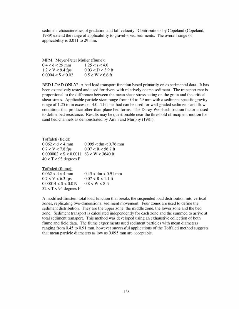
138
sediment characteristics of gradation and fall velocity. Contributions by Copeland (Copeland, 1989) extend the range of applicability to gravel-sized sediments. The overall range of applicability is 0.011 to 29 mm. MPM. Meyer-Peter Muller (flume): 0.4 < d < 29 mm 1.25 < s < 4.0 1.2 < V < 9.4 fps 0.03 < D < 3.9 ft 0.0004 < S < 0.02 0.5 < W < 6.6 ft BED LOAD ONLY! A bed load transport function based primarily on experimental data. It has been extensively tested and used for rivers with relatively coarse sediment. The transport rate is proportional to the difference between the mean shear stress acting on the grain and the critical shear stress. Applicable particle sizes range from 0.4 to 29 mm with a sediment specific gravity range of 1.25 to in excess of 4.0. This method can be used for well-graded sediments and flow conditions that produce other-than-plane bed forms. The Darcy-Weisbach friction factor is used to define bed resistance. Results may be questionable near the threshold of incipient motion for sand bed channels as demonstrated by Amin and Murphy (1981). Toffaleti (field): 0.062 < d < 4 mm 0.095 < dm < 0.76 mm 0.7 < V < 7.8 fps 0.07 < R < 56.7 ft 0.000002 < S < 0.0011 63 < W < 3640 ft 40 < T < 93 degrees F Toffaleti (flume): 0.062 < d < 4 mm 0.45 < dm < 0.91 mm 0.7 < V < 6.3 fps 0.07 < R < 1.1 ft 0.00014 < S < 0.019 0.8 < W < 8 ft 32 < T < 94 degrees F A modified-Einstein total load function that breaks the suspended load distribution into vertical zones, replicating two-dimensional sediment movement. Four zones are used to define the sediment distribution. They are the upper zone, the middle zone, the lower zone and the bed zone. Sediment transport is calculated independently for each zone and the summed to arrive at total sediment transport. This method was developed using an exhaustive collection of both flume and field data. The flume experiments used sediment particles with mean diameters ranging from 0.45 to 0.91 mm, however successful applications of the Toffaleti method suggests that mean particle diameters as low as 0.095 mm are acceptable.
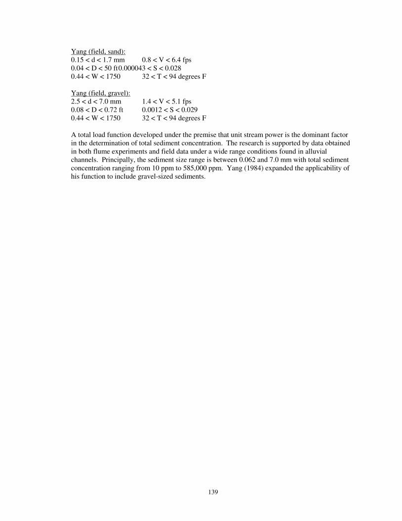
139
Yang (field, sand): 0.15 < d < 1.7 mm 0.8 < V < 6.4 fps 0.04 < D < 50 ft 0.000043 < S < 0.028 0.44 < W < 1750 32 < T < 94 degrees F Yang (field, gravel): 2.5 < d < 7.0 mm 1.4 < V < 5.1 fps 0.08 < D < 0.72 ft 0.0012 < S < 0.029 0.44 < W < 1750 32 < T < 94 degrees F A total load function developed under the premise that unit stream power is the dominant factor in the determination of total sediment concentration. The research is supported by data obtained in both flume experiments and field data under a wide range conditions found in alluvial channels. Principally, the sediment size range is between 0.062 and 7.0 mm with total sediment concentration ranging from 10 ppm to 585,000 ppm. Yang (1984) expanded the applicability of his function to include gravel-sized sediments.
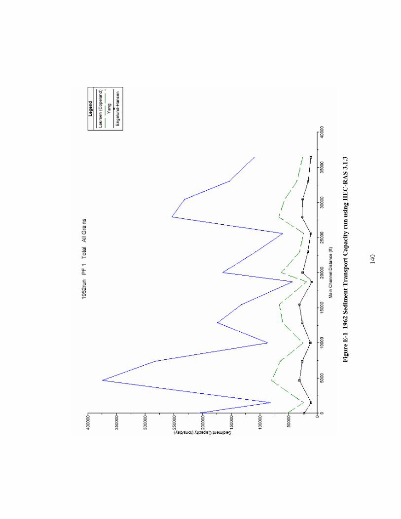
14
0
Fi
gure
E-1
196
2 Se
dim
ent T
rans
port
Cap
acity
run
usi
ng H
EC
-RA
S 3.
1.3
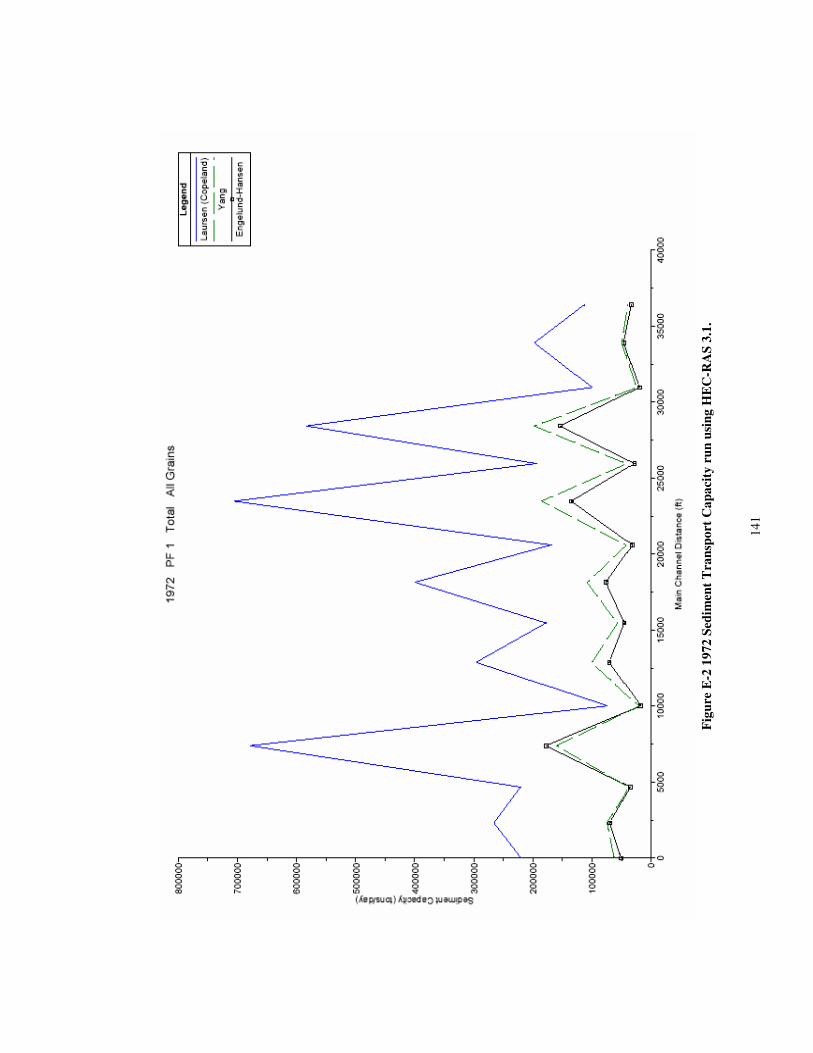
14
1
�Fi
gure
E-2
197
2 Se
dim
ent T
rans
port
Cap
acity
run
usi
ng H
EC
-RA
S 3.
1.
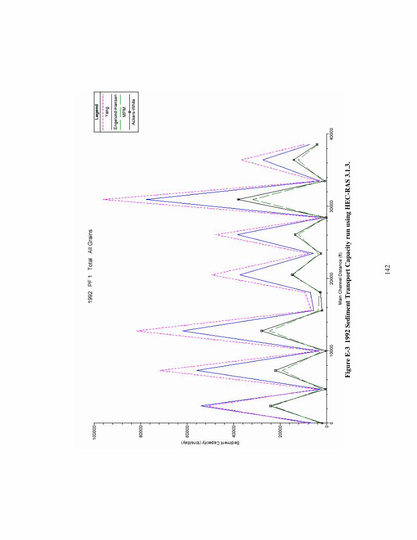
14
2
Fi
gure
E-3
199
2 Se
dim
ent T
rans
port
Cap
acity
run
usi
ng H
EC
-RA
S 3.
1.3.
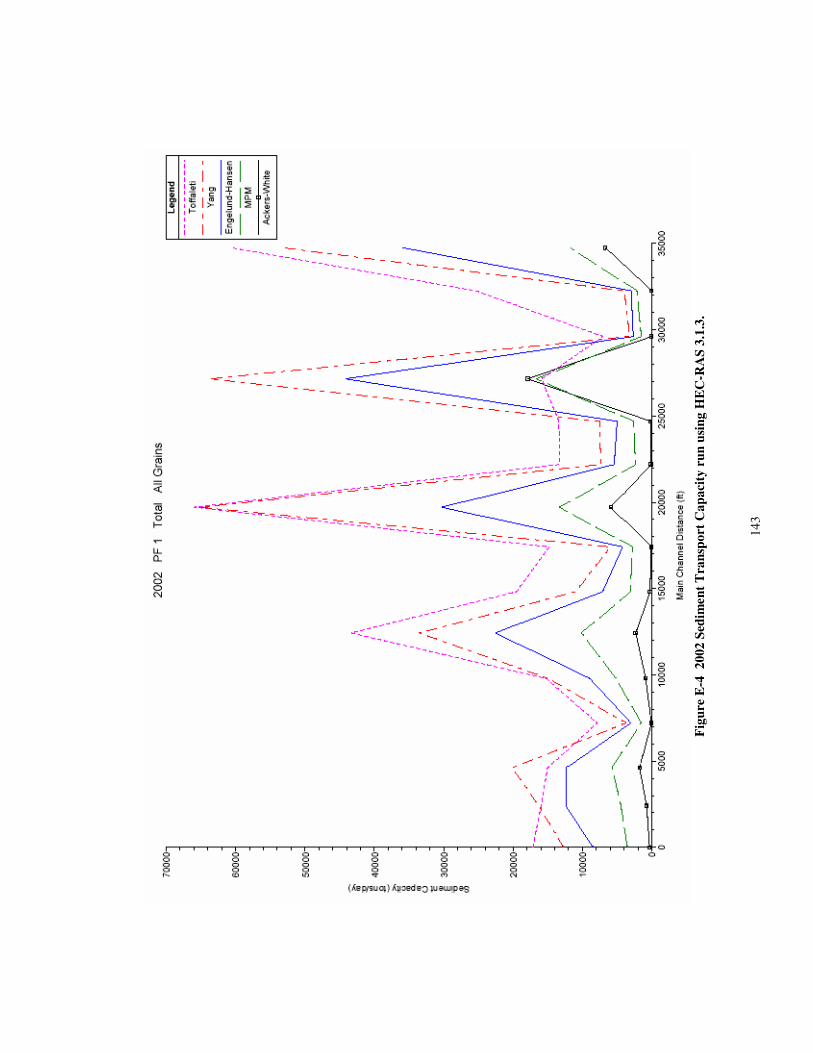
14
3
Fi
gure
E-4
200
2 Se
dim
ent T
rans
port
Cap
acity
run
usi
ng H
EC
-RA
S 3.
1.3.
144
A P P E N D I X F – S T A B L E C H A N N E L A N A L Y S I S
145
F.1 Methods
Two stable channel design programs were available for use: the USACE’s HEC-RAS
3.1.3 and SE-CAP (unpublished by Shih, Watson, and Yang). HEC-RAS’s hydraulic stable
channel design function, based on the SAM Hydraulic Design Package for Flood Control
Channels, was not used for the Cochiti Dam reach. The package uses Brownlie’s flow resistance
and sediment transport equations to produce multiple solutions for the width and slope given at
the input values. Brownlie’s method is for sand-sized bed material, with a maximum d50 of 2
mm. In the Cochiti Dam reach, the d50 is 24 for the total reach, putting it well outside the bounds
of reasonable results.
Instead of SAM, the Visual Basic program SE-CAP was utilized. The program uses
Yang-Copeland’s procedure, which balances sediment transport and capacity by means of the
user’s choice of regime equations. For the Cochiti Dam reach, Ackers and White (1973) and
Meyer-Peter and Muller (1948) were used for stable channel calculations. The program also has
the capacity to use Yang’s gravel (1984), Yang’s sand (1979) (for both low and high
concentrations), Engelund and Hansen (1967), and Bagnold (1966).
Ackers and White’s total load function was chosen because of the higher degree of
compatibility with the channel characteristics. This method has limitations, including the
applicability of the equations to only non-cohesive sands, and a median grain size maximum of 7
mm. The Middle Rio Grande has fairly non-cohesive banks, so this assumption was acceptable.
It was also developed for channel widths much smaller than the study reach. Meyer-Peter and
Muller’s bed load function can handle a median grain size up to 29 mm, making it a better fit for
the bed material in the Cochiti Dam reach. However, this function was also developed for
channel widths much smaller than the Middle Rio Grande.
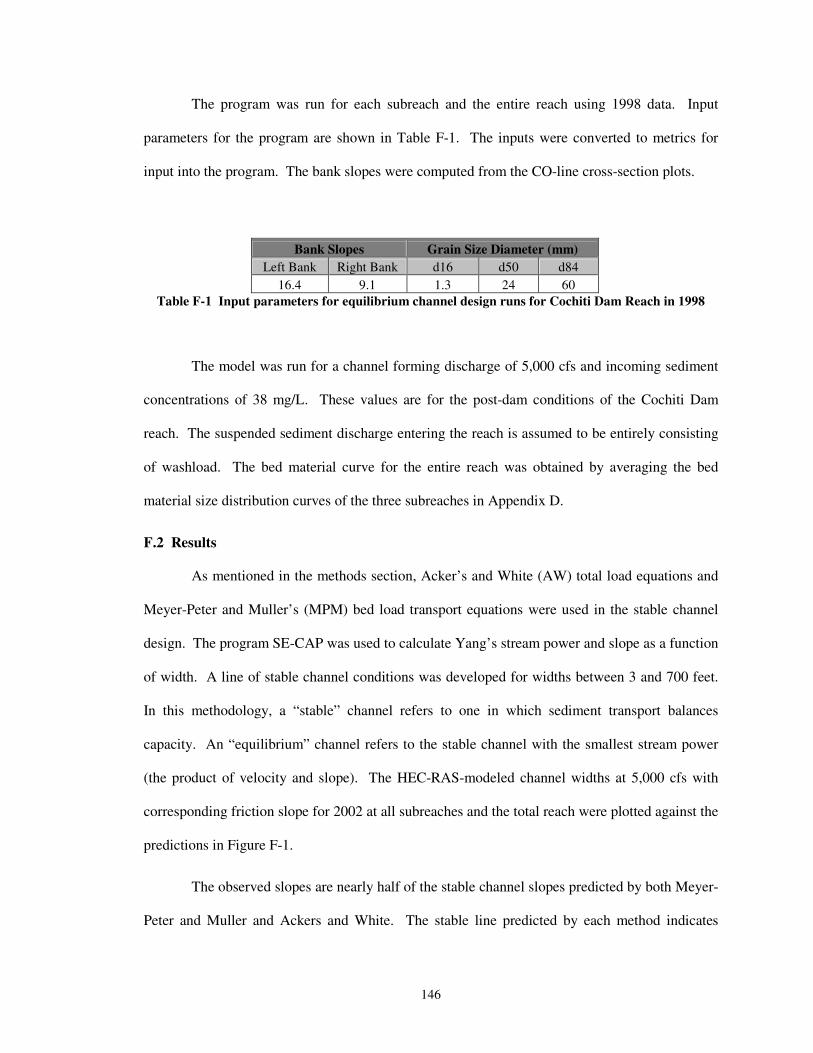
146
The program was run for each subreach and the entire reach using 1998 data. Input
parameters for the program are shown in Table F-1. The inputs were converted to metrics for
input into the program. The bank slopes were computed from the CO-line cross-section plots.
Bank Slopes Grain Size Diameter (mm) Left Bank Right Bank d16 d50 d84
16.4 9.1 1.3 24 60 Table F-1 Input parameters for equilibrium channel design runs for Cochiti Dam Reach in 1998
The model was run for a channel forming discharge of 5,000 cfs and incoming sediment
concentrations of 38 mg/L. These values are for the post-dam conditions of the Cochiti Dam
reach. The suspended sediment discharge entering the reach is assumed to be entirely consisting
of washload. The bed material curve for the entire reach was obtained by averaging the bed
material size distribution curves of the three subreaches in Appendix D.
F.2 Results
As mentioned in the methods section, Acker’s and White (AW) total load equations and
Meyer-Peter and Muller’s (MPM) bed load transport equations were used in the stable channel
design. The program SE-CAP was used to calculate Yang’s stream power and slope as a function
of width. A line of stable channel conditions was developed for widths between 3 and 700 feet.
In this methodology, a “stable” channel refers to one in which sediment transport balances
capacity. An “equilibrium” channel refers to the stable channel with the smallest stream power
(the product of velocity and slope). The HEC-RAS-modeled channel widths at 5,000 cfs with
corresponding friction slope for 2002 at all subreaches and the total reach were plotted against the
predictions in Figure F-1.
The observed slopes are nearly half of the stable channel slopes predicted by both Meyer-
Peter and Muller and Ackers and White. The stable line predicted by each method indicates
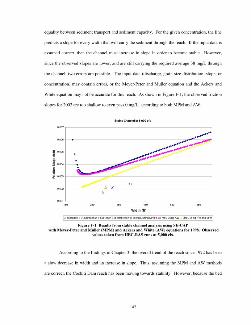
147
equality between sediment transport and sediment capacity. For the given concentration, the line
predicts a slope for every width that will carry the sediment through the reach. If the input data is
assumed correct, then the channel must increase in slope in order to become stable. However,
since the observed slopes are lower, and are still carrying the required average 38 mg/L through
the channel, two errors are possible. The input data (discharge, grain size distribution, slope, or
concentration) may contain errors, or the Meyer-Peter and Muller equation and the Ackers and
White equation may not be accurate for this reach. As shown in Figure F-1, the observed friction
slopes for 2002 are too shallow to even pass 0 mg/L, according to both MPM and AW.
Stable Channel at 5,000 cfs
0.001
0.002
0.003
0.004
0.005
0.006
0.007
150 250 350 450 550 650
Width (ft)
Fric
tion
Slo
pe (f
t/ft)
subreach 1 subreach 2 subreach 3 total reach 38 mg/L using MPM 38 mg/L using AW 0mgL using AW and MPM
Figure F-1 Results from stable channel analysis using SE-CAP
with Meyer-Peter and Muller (MPM) and Ackers and White (AW) equations for 1998. Observed values taken from HEC-RAS runs at 5,000 cfs.
According to the findings in Chapter 3, the overall trend of the reach since 1972 has been
a slow decrease in width and an increase in slope. Thus, assuming the MPM and AW methods
are correct, the Cochiti Dam reach has been moving towards stability. However, because the bed
148
of the Cochiti Dam reach is armored, little degradation is expected in the future. This leaves the
channel little choice but to begin moving laterally, eroding the banks and increasing sinuosity.
�

149
A P P E N D I X G – M I D D L E R I O G R A N D E D A T A B A S E U P D A T E S
150
G.1 Introduction
The Rio Grande Database was a project for the US Bureau of Reclamation started in the
late 1990s. The original database was compiled and discussed by Colorado State University’s
Claudia Leon in her thesis and dissertation. The database included cross-sectional plots,
discharge data, and sediment data for both USGS gaging stations and range-lines along the Rio
Grande. The reach in question stretched from Cochiti Dam to the San Acacia Diversion Dam.
This area is still under study for biological, hydrological, and geological changes.
The MRG Database was compiled in order to facilitate analyses performed to better
understand the changes that are affecting the Middle Rio Grande River. Studies have been done
on meander migration patterns, lateral migration, and general morphology of the river. As more
research is done, the database must be continually added to, organized, and updated.
G.2 The Existing Database
The existing data consisted of several different computer disks, text files, and
spreadsheets, as well as hard-copy data compiled from research projects on several reaches of the
Middle Rio Grande. The existing formal database contained some data analyses done for
research. Some data was raw, and was not yet manipulated.
There were several types of data collected for the MRG Database. Discharge data was
measured along the river at several USGS gaging stations. Instantaneous discharge
measurements were taken at some range-line cross-sections and were available in part from the
USBR.
Cross-sectional measurements of bed elevation, water surface elevation, and thalweg
were taken at several range-lines. Many different cross-sections were collected. The Cochiti
Range-Lines (CO) are the most frequently used by MRG researchers. In addition,
Aggredation/Deggredation (Agg/Deg), Abeyta’s Heading (AH), Bernardo Jack (BJ), Bernalillo
Island (BI), Calabacillas (CA), and Casa Colorada (CC) lines were included.

151
Sediment data was collected at both USGS Gaging Stations as well as at Range-Lines.
Bed Material and Suspended Sediment data were collected from the USGS and the USBR.
Hydraulic Summaries and Total Load Summaries were also collected from the USBR. The
sediment database was expanded with analyses of sediment continuity and sediment transport.
FLO Engineering also contributed sediment data for the early to mid 1990’s. Some sedimentary
and water quality data was received from the EPA as well.
Claudia Leon’s 1998 thesis, “Morphology of the Middle Rio Grande from Cochiti Dam to
Bernalillo Bridge, New Mexico” contains more detailed information about the exact dates and
sources of available data. This thesis is available in the database.
G.3 Database Updates
G.3.1 New Data
New updated information was added through the USGS, the USBR, the EPA, and from
hardcopy reports and files.
The USGS website provided updated discharge data for USGS gaging stations up through
water-year 2002. It also provided some of the needed suspended sediment data for USGS gaging
stations. Particle-size distributions were readily available for each USGS Gaging Station in
service for up to 2004. These were available from the “Water Quality” section of the USGS
website. Suspended Sediment Discharge data was also available through this website; however,
the most recent of this data was 1996.
Cross-sectional data was provided at all available range-lines through spreadsheets and
Auto-CAD drawing files from the USBR-Albuquerque office. Water-surface elevations, bed
elevations, and thalweg depths were also provided by the USBR.
Not every range-line was surveyed each year. The available range-lines varied from
year-to-year, and also varied between discharge, sediment, and cross-sections. CO-lines were the
152
most commonly surveyed and the most widely available; however, even they were not surveyed
each year. These cross-sections were available up to 2002 in a few cases, and at least to 2001 in
most cases.
The EPA’s STORET database was used to obtain a small amount of Albuquerque-area
sediment data as well. Data retrieved from this data-storage facility was sparse and non-uniform.
It was for the most part unusable, however, in the future, more data may become available from
this source.
As recent USBR Hydraulic Modeling Analysis reports been produced, and as recent
theses and dissertations by CSU graduate students have been published, more data has become
available in hard-copy form. The data available in hard-copy form included sediment, discharge,
and cross-sectional figures for the mid to late 90’s. These reports were combed for new data that
was added to the database.
Some data could not be updated. Certain USGS gages have been discontinued or
removed. In addition, the USBR’s Albuquerque office has been missing certain files since their
system upgrade. New discharge and velocity measurements at range-lines below Bernalillo
Bridge were unavailable. In addition, suspended sediment data was sparse and had several gaps
in the records. The Albuquerque office staff was unaware of the missing recent data until this
updating project brought their attention to it. As they find the missing data, it will be sent to be
added to the updates.
G.3.2 Database Organization
New information was added into the existing data files. Any duplicate data was checked
for consistency of numbers. In some older files, the data was based on estimates or on “real-
time” data instead of official daily values. These values were used because the official values
were unavailable. During the updates, the estimates or “real-time” data was replaced with the
153
official values if they were available. This kept the database from having too many unnecessary
duplicate entries.
Some data files overlap dates. It was necessary to keep these duplicate files because
different analyses were performed on each set of data. In some cases, an original, raw data set
was kept for further or new analyses.
After the new information was obtained, it was organized into the database by reach and
then by sub reach. The entire database was then reorganized for clarity and ease of use. A
webpage interface was created to tie the folders together.
In the case that a researcher needed all discharge data for the Corrales reach, she could
simply go directly to that folder. Any HEC-RAS data and analyses for the Bernardo reach could
be easily accessed in the same way. The overall organization is shown in Figures G-1 through
G-5. Finally, a “Readme” file was added to each subfolder to describe the contents of each
section.
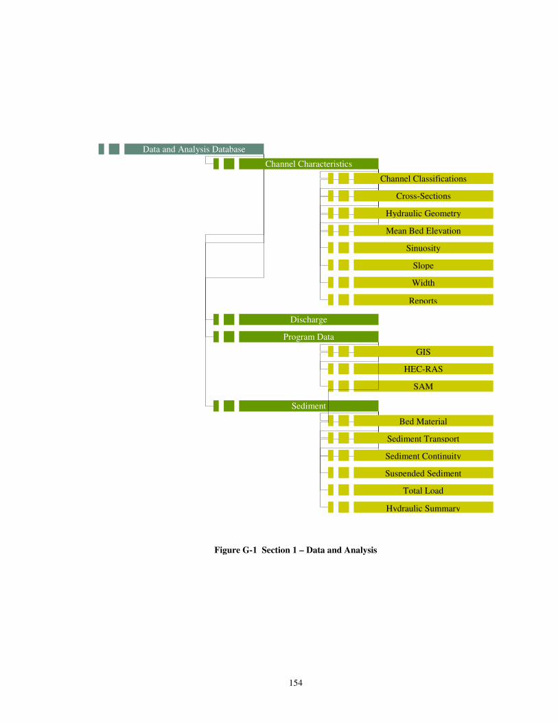
154
Figure G-1 Section 1 – Data and Analysis
Data and Analysis Database
Channel Characteristics
Discharge
Program Data
Sediment
Channel Classifications
Cross-Sections
Hydraulic Geometry
Mean Bed Elevation
Sinuosity
Slope
GIS
HEC-RAS
SAM
Bed Material
Sediment Transport
Sediment Continuity
Suspended Sediment
Width
Total Load
Hydraulic Summary
Reports
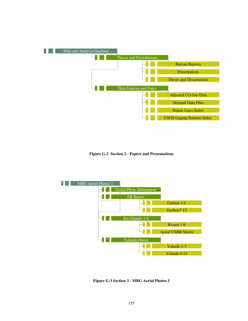
155
Figure G-2 Section 2 - Papers and Presentations
Figure G-3 Section 3 - MRG Aerial Photos 1
MRG Aerial Photos 1 Aerial Photo Information
EB Reserv
Rio Grande 1-9
Valarde-Otowi
Riogra 1-9
Aerial USBR Sheets
Valarde 1-7
Valarde 8-14
Gorbon 1-6
Gorbon7-12
Data and Analysis Database
Theses and Presentations
Data Sources and Dates
Bureau Reports
Presentations
Theses and Dissertations
Adjusted CO-line Data
Original Data Files
Range Lines Index
USGS Gaging Stations Index
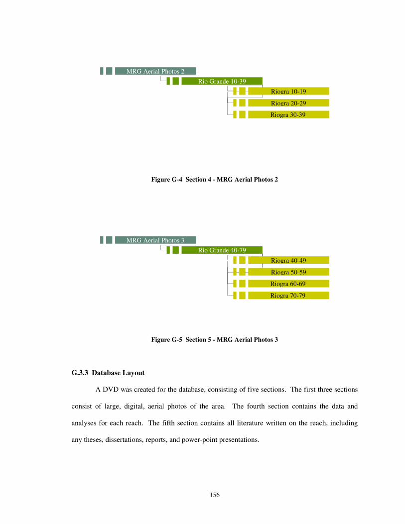
156
�
Figure G-4 Section 4 - MRG Aerial Photos 2
Figure G-5 Section 5 - MRG Aerial Photos 3
G.3.3 Database Layout
A DVD was created for the database, consisting of five sections. The first three sections
consist of large, digital, aerial photos of the area. The fourth section contains the data and
analyses for each reach. The fifth section contains all literature written on the reach, including
any theses, dissertations, reports, and power-point presentations.
MRG Aerial Photos 3 Rio Grande 40-79
Riogra 40-49
Riogra 50-59
Riogra 60-69
Riogra 70-79
MRG Aerial Photos 2
Rio Grande 10-39
Riogra 10-19
Riogra 20-29
Riogra 30-39
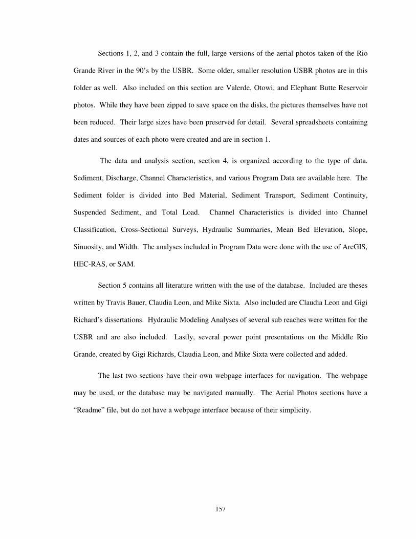
157
Sections 1, 2, and 3 contain the full, large versions of the aerial photos taken of the Rio
Grande River in the 90’s by the USBR. Some older, smaller resolution USBR photos are in this
folder as well. Also included on this section are Valerde, Otowi, and Elephant Butte Reservoir
photos. While they have been zipped to save space on the disks, the pictures themselves have not
been reduced. Their large sizes have been preserved for detail. Several spreadsheets containing
dates and sources of each photo were created and are in section 1.
The data and analysis section, section 4, is organized according to the type of data.
Sediment, Discharge, Channel Characteristics, and various Program Data are available here. The
Sediment folder is divided into Bed Material, Sediment Transport, Sediment Continuity,
Suspended Sediment, and Total Load. Channel Characteristics is divided into Channel
Classification, Cross-Sectional Surveys, Hydraulic Summaries, Mean Bed Elevation, Slope,
Sinuosity, and Width. The analyses included in Program Data were done with the use of ArcGIS,
HEC-RAS, or SAM.
Section 5 contains all literature written with the use of the database. Included are theses
written by Travis Bauer, Claudia Leon, and Mike Sixta. Also included are Claudia Leon and Gigi
Richard’s dissertations. Hydraulic Modeling Analyses of several sub reaches were written for the
USBR and are also included. Lastly, several power point presentations on the Middle Rio
Grande, created by Gigi Richards, Claudia Leon, and Mike Sixta were collected and added.
The last two sections have their own webpage interfaces for navigation. The webpage
may be used, or the database may be navigated manually. The Aerial Photos sections have a
“Readme” file, but do not have a webpage interface because of their simplicity.
�
�
158
G.4 MRG Database DVD
The database DVD is the final product of this project. The DVD can be navigated using
the webpage interfaces included, or it can be explored manually through each folder. A
“Readme” file is included in each folder to facilitate use of the database for those who have not
read this report.
�