Hydraulic Behavior and Performance of Breastshot WaterWheels for Different Numbers of Blades

Emanuele Quaranta1 and Roberto Revelli2

Abstract: Thanks to their efficiency and simplicity of contruction, breastshot water wheels represent an attractive low head hydropowerconverter. In this work, a breastshot wheel is investigated by numerical simulations, and the results are validated with experimental tests.The average discrepancy between the numerical shaft torque and the experimental torque is lower than 5%. The numerical model is thenused to investigate the performance and the hydraulic behavior of the wheel for different numbers of blades (16, 32, 48, and 64 blades)and at different hydraulic conditions. The increase in efficiency from 16 blades to the optimal blades number ranges between 12 to 16% infunction of the hydraulic conditions. Empirical laws are also reported to quantify the improvement in efficiency with the blades number.These laws can support the design process of similar breastshot water wheels. The optimal blades number for this kind of wheel isidentified in 48. DOI: 10.1061/(ASCE)HY.1943-7900.0001229. © 2016 American Society of Civil Engineers.

Author keywords: Blades number; Computational fluid dynamics (CFD); Hydropower; Mini-hydro; Water wheels.

Introduction

In the European Commission legislations, electricity productionin large scale from renewable energy sources has become a majorpurpose for meeting the important renewable energy targets andto limit greenhouse gas emissions. As a consequence, a new andwide interest on renewable sources is spreading in Europe and alsoworldwide, especially the energy production by wind, solar, andhydro power. With respect to wind and solar energy production,hydroelectricity generally exhibits some advantages. Hydro plantsare more responsive to load management requirements (they canbe managed by human control easier), and hydro output is morepredictable than solar and wind output. The drawback of wind andsolar resources is their variability in time, which introduces theneed of additional storage capacity (Bodis et al. 2014).

However, in Europe, sites suitable for large plants have alreadybeen exploited, and their environmental impacts are generally notwell accepted. Mini/micro hydropower plants (net power inputlower than 1 MW and 100 kW, respectively) are instead more sus-tainable and eco-friendly. They are becoming more attractive thanbig power plants, mainly in rural and decentralized areas for self-sustainment. In the industrialized countries, mini/micro hydro-power is also useful for meeting the nonfossil fuel targets, whereasin developing countries, it may contribute to satisfy the rising de-mand of decentralized electricity.

However, most low-head and low-discharge sites are currentlynot exploited because standard turbines cannot be employedeconomically in such conditions. As a consequence, there exists a

demand for a cost-effective low-head hydropower converter, andwater wheels may represent an attractive solution to this problem(Bozhinova et al. 2013; Müller and Kauppert 2004). This is espe-cially supported by their fast payback periods and simplicity ofconstruction. Water wheels fit well into the ecosystems; thus, theyare considered not out of place when installed along a river. Waterwheels can also contribute to the preservation of the cultural her-itage (the restoration of old water mills), hence to the developmentof eco-tourism and promotion of social activities. Therefore, theemployment of classical water wheels for the generation of renew-able energy from water is becoming a cost-effective and sustainablesolution in the mini/micro hydro field.

Water wheels were introduced more than 2,000 years ago inorder to produce energy, pump water, grind grain, forge iron, sawwood and stones, work with metal, and tan leather. Nowadays, thetotal number of existing historic small and micro hydropower sitesin Europe is estimated to be around 350,000 (ESHA 2014).

The oldest water wheel had a vertical axle, whereas the firstkind, with a horizontal axle, was the stream water wheel (alreadydescribed by Vitruvius in 27 BC). In stream water wheels, nowa-days employed in flowing water and in sites with null or very lowheads, the water flows below the wheel (Muller et al. 2007). Streamwheels are impulse machines; thus, the kinetic energy of water ismainly exploited, although recent studies have introduced consid-erable improvement, where also the hydrostatic force is employed(Gotoh 2001).

In 1759, John Smeaton published experimental data (Capecchi2013) demonstrating the higher efficiency of gravity wheels overthe efficiency of impulse stream wheels. In gravity water wheels,the water acts by its weight, and the potential energy of water ismainly exploited. The stream kinetic energy can give its contribu-tion during the filling time, when the water fills into the bucketsand impacts against the blades. In the eighteenth and nineteenthcenturies, some theories and experimental tests on water wheelswere performed (Poncelet 1843; Morin and Morris 1843; Weisbach1849; Bach 1886; Chaudy 1896; Garuffa 1897; Church 1914).However, theories were generally developed separately from exper-imental tests. Theories were often not validated, and several pre-scriptions on water wheels’ design were empirical and not basedon scientific evidence. Furthermore, the experimental tests were

1Ph.D. Candidate, Dept. of Environment, Land and InfrastructureEngineering, Politecnico di Torino, DIATI, Corso Duca degli Abruzzi 24,10129 Torino, Italia (corresponding author). E-mail: emanuele.quaranta@polito.it; quarantaemanuele@yahoo.it

2Professor, Dept. of Environment, Land and Infrastructure Engineering,Politecnico di Torino, DIATI, Corso Duca degli Abruzzi 24, 10129 Torino,Italia. E-mail: roberto.revelli@polito.it

Note. This manuscript was submitted on December 5, 2015; approvedon June 21, 2016; published online on August 16, 2016. Discussion per-iod open until January 16, 2017; separate discussions must be submittedfor individual papers. This paper is part of the Journal of HydraulicEngineering, © ASCE, ISSN 0733-9429.

© ASCE 04016072-1 J. Hydraul. Eng.

J. Hydraul. Eng., 04016072

Dow

nloa

ded

from

asc

elib

rary

.org

by

DIP

Idr

aulic

a/T

rasp

orti

E o

n 08

/19/

16. C

opyr

ight

ASC

E. F

or p

erso

nal u

se o

nly;

all

righ

ts r

eser

ved.

carried out more than one century ago, with several uncertainties.At the end of the nineteenth century, the advent of modern turbines(such as Pelton, Francis, and Kaplan turbines, employed in big hy-droelectric plants) replaced the classical water wheels, and energyproduction from low head sites was practically forgotten.

Nowadays, because of the new interest in mini hydropower asdescribed previously, the scientific research on water wheels isexperiencing a revival. However, the engineering information onwater wheels is ancient (hundreds of years), and there are still sev-eral uncertainties concerning their optimal working conditions, op-timal geometric design, and fluid dynamic behavior. Hence, furtherwork is necessary.

Types of Gravity Water Wheels

Among gravity wheels, overshot, breastshot, and undershot waterwheels can be identified, depending on the water entry point withrespect to the wheel. In gravity wheels, the potential energy ofwater is mainly exploited, whereas the flow kinetic energy effec-tively exploited by the wheel depends strictly on the hydraulicimpact conditions and on the blades’ design (Quaranta and Revelli2015b), such as blades number and shape.

In overshot wheels (Quaranta and Revelli 2015a), the waterfills the buckets along the downstream side of the wheel, enteringfrom the top of the wheel. In breastshot water wheels (Quaranta andRevelli 2015b), the water enters into the wheel approximately incorrespondence of the rotation axle. They can be divided in highand low breastshot wheels, when the water enters into the cells overthe axle or below it, respectively. Breastshot wheels rotate in thereverse direction with respect to overshot wheels. The water is car-ried by the buckets to the outlet, downstream of the wheel, where itis released into the tailrace. Low breastshot wheels employed atvery low head sites are called undershot water wheels (Quarantaand Müller 2016). In particular, breastshot water wheels are usedin sites with head differences between 1.5 to 4 m, which are typicalsituations that can be found, for example, in irrigation canals.However, the most of the available design information is ancient(hundreds of years) (Poncelet 1843; Morin and Morris 1843;Weisbach 1849; Bach 1886; Chaudy 1896; Garuffa 1897; Church1914), and very few fluid dynamics evidence is available in theliterature, especially on the effects of the blades number on theirperformance.

Scope of the Paper

Based on the scientific gaps exposed in the previous sections, themain purpose of the present paper is the investigation of the effectof the blades number on the performance of a breastshot waterwheel and to study, in more detail, the fluid dynamic interactionwith the flow. The investigated wheel is 2.12 m in diameter, andit is a physical scaled model of a real one. The wheel will be betterdescribed in the “Method” section.

Considering that an attractive opportunity for studying hy-draulic problems and hydraulic machinery is now represented bycomputational fluid dynamics (CFD) simulations, CFD tools areused in this work to achieve the purpose mentioned previously.In the last decades, the employment of CFD tools for solving fluiddynamic problems has been developing more and more becauseCFD tools enable access to local flow properties with relatively lowcosts and with a substantial reduction in the experimental expendi-ture. For these motivations, fluid dynamic simulations may alsorepresent a suitable and efficient method to investigate the hy-draulic behavior of water wheels, obtaining useful information fortheir design. The involved phenomena are generally quite complex

because they involve an unsteady 3D turbulent regime, a biphasesformulation (a primary and a secondary phase, air and water, re-spectively), the gravity external force, and the moving and curvedbody of the wheel.

CFD simulations for horizontal water wheels (Pujol et al. 2010)and stream wheels (Liu and Peymani 2015; Akinyemi and Liu2015a, b) have been already presented in scientific journals,whereas to the best of the authors’ knowledge, CFD results forgravity water wheels can rarely be found. By the present work,the suitability of fluid dynamic simulations will be hence demon-strated also for breastshot water wheels; the numerical results arecompared with those obtained by testing the same breastshot wheel(with 32 blades) in the laboratory, showing that the numerical sol-ution can be considered accurate.

The investigation of the optimal blades number for breastshotwater wheels is justified by the fact that, in the scientific literature,the effect of the blades number on the performance of water wheelshas been investigated mainly for stream water wheels. In Lutheret al. (2013), the efficiency of a stream wheel with straight bladesincreased from 4 to 8 paddles, whereas in Tevata and Chainarong(2011), a water wheel with straight blades has been tested, and theefficiency decreased passing from 6 to 12 blades. The global behav-ior deducted from the last two papers suggests that for streamwheels, an optimum blades number can be identified. Moreover, inMüller et al. (2010), it is illustrated that the efficiency of a floatingwater wheel increased from 8 to 24 blades, with a substantial im-provement from 8 to 12; the result also suggests that, in this case, anoptimal blades number exists. Considering the previous deductions,the authors are, hence, stimulated to achieve similar results also forbreastshot water wheels.

In the following sections, the numerical setup and experimentalmethod will be described. The numerical results will be comparedwith the experimental ones and discussed in detail. Practical engi-neering information concerning optimal numbers of blades for sim-ilar breastshot wheels in different hydraulic conditions will bereported.

Method

A breastshot water wheel in an open channel was numerically in-vestigated by CFD tools, in order to understand the effect of theblades number on its hydraulic behavior and performance, thus onthe power output and efficiency. The diameter and the width of thetested wheel are D ¼ 2.12 m and b ¼ 0.65 m, respectively, andthe height of the blades is 0.29 m; the investigated numbers of thecurved blades are nb ¼ 16; 32; 48; 64. A physical model of thesame dimension, with nb ¼ 32 and a total weight of W ≃ 3500 N,has also been installed in the Laboratory of Hydraulics at Politec-nico di Torino, and the experimental results are used to validate thenumerical ones.

CFD Model: Geometry and Mesh

The computational domain is constituted of three subdomains: thestationary domain of the channel, which conveys water to thewheel; the rotating domain of the wheel, which interacts withthe channel; and stationary domain outside of the wheel, filled onlywith air. A sliding mesh approach was used. The stationary air do-main is subdivided in an internal domain, in contact with the wheel,and an external domain. The latter has the scope to locate the boun-dary conditions sufficiently far away from the wheel and to stabilizethe solution (Fig. 1).

The channel and the wheel are meshed with tetrahedral ele-ments, whose dimensions range between 0.01 and 0.02 m (a mesh

© ASCE 04016072-2 J. Hydraul. Eng.

J. Hydraul. Eng., 04016072

Dow

nloa

ded

from

asc

elib

rary

.org

by

DIP

Idr

aulic

a/T

rasp

orti

E o

n 08

/19/

16. C

opyr

ight

ASC

E. F

or p

erso

nal u

se o

nly;

all

righ

ts r

eser

ved.

size of 0.02 m in the buckets ensures a mesh independent solution,as illustrated in the “Results” section). The stationary air domainis meshed with tetrahedron and cubic elements, whose dimensionsrange between 0.02 m near the wheel and the channel, up to 0.1 mat the boundaries of the external domain. The coarse mesh near theboundaries of the external domain does not affect the interactionbetween water and wheel. In order to reduce computational timewithout losing accuracy in the solution, it is not necessary to sim-ulate the whole domain of the wheel (2π rad); half a wheel is suf-ficient to simulate the wheel-stream interaction (Barstad 2012), andthe remaining half portion of the wheel is simulated with a coarsermesh and without blades (reducing the domain complexity). Thefinal mesh has 1.3 million cells (Fig. 2).

CFD Model: Simulation Setup

The Reynolds Averaged Navier–Stokes (RANS) equations wereemployed for solving the flow field in the computational domains.The RANS equations include three momentum equations (oneequation for each Cartesian coordinate) and the continuity equa-tion. In the RANS equations, each variable y (pressure and thevelocity) is decomposed in a time averaged value y and a fluctuat-ing component y 0, the latter representing the difference between theinstantaneous value of variable y and the time averaged value y.

Because the problem involves two phases (air and water,separated by a free surface), it is essential to add to the RANSequations an additional continuity equation to solve the multiphaseproblem. The additional continuity equation allows to determinein each cell of the domain the fraction volume of water and air.Knowing the volume fraction of each phase in all the cells of thedomain, the physical properties (viscosity and density) of the mix-ture can be quantified [Eqs. (2) and (3)] and used to solve theRANS equations of the mixture.

The volume of fluid method (VOF) was used to solve themultiphase problem. This method can be used with two or moreimmiscible fluids. A continuity equation for phase q is solved,tracking the volume fraction αq of the phase throughout thedomain [Eq. (1)]

∂αq

∂t þ ∂ðαquiÞ∂xi þ ∂ðαqujÞ

∂xj þ ∂ðαquwÞ∂xw ¼ 0 ð1Þ

Fig. 1. Computational domain and the boundary conditions (B.C.) of the numerical model; the figure represents a longitudinal section on the verticalsymmetry plane; some representative dimensions are reported (m)

Fig. 2. Computational meshed domain; the figure represents a long-itudinal section on the vertical symmetry plane; the portion of the wheelwith the blades is meshed with finer elements, which after approxi-mately 1 s, begin to interact with the stream

© ASCE 04016072-3 J. Hydraul. Eng.

J. Hydraul. Eng., 04016072

Dow

nloa

ded

from

asc

elib

rary

.org

by

DIP

Idr

aulic

a/T

rasp

orti

E o

n 08

/19/

16. C

opyr

ight

ASC

E. F

or p

erso

nal u

se o

nly;

all

righ

ts r

eser

ved.

where αq = volume fraction of phase q (the so called secondaryphase, that, in this case, is represented by water) in each cell;αq ¼ 1 means that the cell is filled of water; αq ¼ 0 means thatthe cell is filled of air; 0 < αq < 1 means that the cell is near thefree surface; xi, xj, and xw = directions of the Cartesian referencecoordinate system; and generic uy = time averaged velocity of themixture [Eq. (5)] in the xy direction. Once the volume fraction ofphase q is identified, the volume fraction of phase p (air) is calcu-lated by αp ¼ 1 − αq.

For the solution of the VOF equation, an implicit interpolationscheme was used, coupled with the level-set method, which is awell-established interface-tracking method for computing two-phases flows with topologically complex interfaces. Because thelevel-set function is smooth and continuous (Osher and Sethian1988), its spatial gradients can be accurately calculated. Therefore,the interface curvature and surface tension forces caused by thecurvature are estimated accurately. However, the level-set methodhas a deficiency in preserving volume conservation (Olsson et al.2007). On the other hand, the VOF method is naturally volume-conserved; it calculates the volume fraction of a particular phasein each cell, instead of the interface itself. The weakness of theVOF method is the calculation of its spatial derivatives becausethe volume fraction of a particular phase is discontinuous across theinterface. To overcome the lack of the level-set method and thelack of the VOF method, a coupled level-set and VOF approachwas used.

After the determination of fraction volume αq and αp of thephases in each cell, the mixture properties are calculated:

ρ ¼ αqρq þ αpρp ð2Þ

μ ¼ αqμq þ αpμp ð3Þ

where ρ and μ = density and dynamic viscosity of the mixture, re-spectively, and ρy and μy = properties of the generic phase y.

The RANS continuity and momentum equations for the mix-ture are then solved. For an incompressible fluid the continuityequation is

∂ui∂xi þ

∂uj∂xj þ

∂uw∂xw ¼ 0 ð4Þ

The momentum equation for the mixture in direction xi, is

ρ

�∂ui∂t þ ui

∂ui∂xi þ uj

∂ui∂xj þ uw

∂ui∂xw

�

¼ ρgi − ∂p∂xi þ μ∇2ui þ

∂∂xi ð−ρu

0iu 0

iÞ þ∂∂xj ð−ρu

0iu 0

jÞ

þ ∂∂xw ð−ρu

0iu 0

wÞ ð5Þ

where ρ and μ = density and dynamic viscosity of the mixture; g =gravitational acceleration; p = time averaged pressure; and ui =mixture time averaged velocity along the direction xi. Analogousmomentum equations are solved along the direction xj and xw.

The terms ρu 0iu 0

j are the Reynolds turbulent stresses, and theycan be expressed as

τ i;j ¼ −ρu 0iu 0

j ¼ μt

�∂ui∂xj þ

∂uj∂xi

�− 2

3ρkδij ð6Þ

where μt = turbulent viscosity; k = turbulent kinetic energy; andδij = Kronecker delta.

The turbulence viscosity is modeled using the shear-stress trans-port (SST) k − ω model (Menter 1994). In this model, the turbulentviscosity is expressed as a function of the turbulent kinetic energy kand the specific dissipation rate ω ¼ ϵ=k, where ϵ is the turbulencedissipation. The solution of two evolution equations (for predictingk and ω) determines the turbulent viscosity μt, that resolves theclosure problem of the RANS formulation

μt ¼ ρkω

1

max�

1α� ; SF

a1ω

� ð7Þ

where α� damps the turbulent viscosity causing a low-Reynoldsnumber correction; a1 = constant; S = strain rate magnitude; andF = blending function. The SST turbulence model is known to per-form better than the k − ϵ model in regions with adverse pressuregradients and separations and near the walls (Menter 1994).

The k − ω equations are, respectively

∂ðρkÞ∂t þ ∂ðρkuiÞ

∂xi þ ∂ðρkujÞ∂xj þ ∂ðρkuwÞ

∂xw¼ ∂

∂xi�Γk

∂k∂xi

�þ ∂∂xj

�Γk

∂k∂xj

�

þ ∂∂xw

�Γk

∂k∂xw

�þ Gk þ Yk þ Sk ð8Þ

∂ðρωÞ∂t þ ∂ðρωuiÞ

∂xi þ ∂ðρωujÞ∂xj þ ∂ðρωuwÞ

∂xw¼ ∂

∂xi�Γω

∂ω∂xi

�þ ∂∂xj

�Γω

∂ω∂xj

�

þ ∂∂xw

�Γω

∂ω∂xw

�þGω þ Yω þ Sω þDω ð9Þ

where G = generation of turbulent kinetic energy (or generationof dissipation); Γ = effective diffusivity; Y = dissipation of k (or ω);D = cross-diffusion term; and S = eventual user-defined sourceterms.

In free-surface flows, a high-velocity gradient at the interfacebetween two fluids results in high turbulence generation, in boththe phases. Therefore, the turbulence damping option is suggestedin the interface area to model such flows correctly. The curvaturecorrection is suggested to sensitize the model to streamline curva-ture and system rotation.

The pressure-velocity coupling was solved by the Piso scheme,and the spatial discretizations were made by the Presto scheme forpressure and the Second-Order Upwind scheme for momentumand turbulent kinetic energy. The modified High Resolution Inter-face Capturing scheme (HRIC) is used for computing the volumefraction (which, in this case, allowed adopting a larger temporaldiscretization).

The time step chosen for the unsteady simulation was8 · 10−4 s, although during some simulations, it was reduced to5 · 10−4 s. A Second-Order Implicit scheme in time was used forthe temporal discretization; 20 inner iterations were carried out be-tween two consecutive time steps for the pressure-velocity solving.

Boundary Conditions

The mass flow rate was imposed at the inlet of the channel, speci-fying the free-surface level and the quantity of entry flow rate inkg=s. At the inlet, a fixed value of the turbulence intensity I ¼ 0.05(a turbulence intensity of 0.01 or less is generally considered low,and turbulence intensity greater than 0.1 is considered high) and a

© ASCE 04016072-4 J. Hydraul. Eng.

J. Hydraul. Eng., 04016072

Dow

nloa

ded

from

asc

elib

rary

.org

by

DIP

Idr

aulic

a/T

rasp

orti

E o

n 08

/19/

16. C

opyr

ight

ASC

E. F

or p

erso

nal u

se o

nly;

all

righ

ts r

eser

ved.

fixed value of the turbulent viscosity ratio μt=μ ¼ 10 were im-posed, where μ is the dynamic viscosity of water; both the quan-tities are fixed by default, and a literature review confirms them(Pujol et al. 2010). At the outlet of the channel and at the externalsurfaces of the external air domain, the pressure outlet option wasadopted ensuring the atmospheric pressure. At the top of theexternal domain, the symmetry boundary condition was imposed(although this condition is not physical, it gives more stability tothe solution, and it does not affect the interaction between waterand wheel). Because the wheel is symmetric with respect to a ver-tical plane perpendicular to the rotation axle passing for the axlecenter, the symmetry boundary condition was imposed on this sur-face, and only one half of the wheel is simulated, saving computa-tional time. At the walls (blades surfaces, channel’s bed and wheel)the no-slip boundary condition was imposed (Fig. 1).

Experimental Tests and Cases Selection for theNumerical Analyses

A 1:2 steel scale model of a real breastshot wheel has been installedin the Laboratory of Hydraulics at Politecnico di Torino (Fig. 3),with Froude similarity. The diameter of the wheel wasD ¼ 2.12 m,and the width was b ¼ 0.65 m; the number of the curved blades,fastened to the lateral shrouds, was nb ¼ 32, and the weight of thewheel was W ≃ 3500 N. A sluice gate was installed 0.7 m (Fig. 1)upstream of the entry point of water to the wheel. During experi-ments, the working conditions could be varied acting on theentry flow rate (Q) by a pump (0.02 < Q < 0.1 m3=s, with ΔQ ¼0.01 m3=s), the entry stream velocity to the wheel by the sluicegate (sluice gate opening 0.05 < a < 0.15 m, Δa ¼ 0.025 m) andthe wheel rotational speed (N) by an electromagnetic brake (0.2 <N < 2.1 rad=s).

The flow rate was detected by a flowmeter with an accuracyof �0.5 · 10−3 m3=s, whereas a torque transducer registered theoutput torque Cexp at the shaft with a precision of �6 Nm. Thewheel was connected to a brake system, constituted of a generatorand a resistor. An electrical energy analyzer and a control of theelectrical resistance were installed to manage the electrical poweroutput of the generator and the load on the wheel, regulating thewheel angular velocity. Between the wheel and the brake, a gearboxwas installed for providing an optimum speed and torque range onthe generator shaft. Along the shaft, an inductive proximity sensor

was installed in order to acquire the wheel rotational speed. Thewheel rotational speed was measured by the internal clock ofthe acquisition board, which could discretize the output signal fre-quency of the proximity sensor until 100 MHz. The experimentalpower output Pexp ¼ Cexp · N could be determined, multiplying thetorqueCexp for the angular velocityN. The power accuracy dependsmainly on the torque transducer accuracy because the wheel veloc-ity is monitored with very high rigor (the power accuracy is≃� 6 · Pexp · C−1

exp).The power input to the wheel was evaluated by the following

equation:

Pin ¼ ρgQH ð10Þwhere ρ ¼ 1000 kg=m3 = density of water; Q = total flow rate; andH = head difference available to the wheel (energy head differencebetween the inlet and the exit point, Fig. 1). The efficiency can beexpressed as the ratio of the power output to the power input

η ¼ Pexp

Pinð11Þ

For further information on the experimental results and setup, referto Quaranta and Revelli (2015b) and Vidali et al. (2016), where theexperiments are described in detail. The experimental results areused to validate the numerical ones, using as control parameterthe shaft torque.

In the numerical simulations, a sluice gate opening was fixed,and three particular cases were chosen, each one with a specificflow rate and wheel rotational speed. An opening of 0.075 m wasadopted: (1) in order to achieve high stream velocity interactingwith the blades (the power output increases with the reductionin the sluice gate opening, and for this sluice gate opening, a widerrange of flow rates has been experimentally investigated with re-spect to the sluice gate opening a ¼ 0.05 m); (2) flow rates of0.05 m3=s (Case 1), 0.06 m3=s (Case 2), and 0.07 m3=s (case3) were adopted; and (3) wheel rotational speeds were chosen inorder to investigate optimal working conditions of the breastshotwater wheel (0.78, 0.79, and 0.89 rad=s, respectively). Thesevelocities are also similar to compare the performance at differentflow rates and approximately constant rotational speed. In theseconditions, the water depth at a location 0.27 m upstream of thewheel was 0.05 m.

In order to generalize the achieved results, the investigatedhydraulic conditions are also presented in dimensionless terms byusing the normalized head, normalized rotational speed, and nor-malized flow rate.

The normalized head is defined as

H� ¼ HD

ð12Þ

which is the ratio of the energy head (in meter) to the wheeldiameter.

The normalized flow rate is defined as

Q� ¼ QðN · RÞH2

ð13Þ

as defined in Vidali et al. (2016) (using the energy head differenceH instead of the geometric head difference between the upstreamand downstream channel’s bed).

The normalized rotational speed is defined as

N� ¼ N · Rffiffiffiffiffiffiffiffiffiffiffi2 gH

p ð14Þ

which is normalized on the Torricelli termffiffiffiffiffiffiffiffiffiffiffi2 gH

p, which repre-

sents the absolute velocity of a particle falling from a total height

Fig. 3. Experimental water wheel; at the shaft, the cylinder on the left isthe generator, whereas the rectangular box is the gearbox; the wheel’sdiameter is 2.12 m

© ASCE 04016072-5 J. Hydraul. Eng.

J. Hydraul. Eng., 04016072

Dow

nloa

ded

from

asc

elib

rary

.org

by

DIP

Idr

aulic

a/T

rasp

orti

E o

n 08

/19/

16. C

opyr

ight

ASC

E. F

or p

erso

nal u

se o

nly;

all

righ

ts r

eser

ved.

equal to H. In Quaranta and Revelli (2016), the optimal range ofnormalized velocity, defined as in Eq. (14), was between 0.3 to 0.4.Therefore, in the present paper, normalized velocities of approxi-mately 0.3 were chosen. Table 1 reports the investigated workingconditions.

Once the numerical model with 32 blades is validated, it is pos-sible to obtain a performance optimization by changing the numberof blades in the geometry setup.

Results and Discussion

Post Processing of the Results

In the present study, the aim of the CFD simulations is to determinehow the performance of the breastshot water wheel is affected bythe blades number. Each time step took approximately 2 min in aprocessor at 2.40 GHz with 8 Gb RAM, for a total time of approx-imately 7–10 days for simulation.

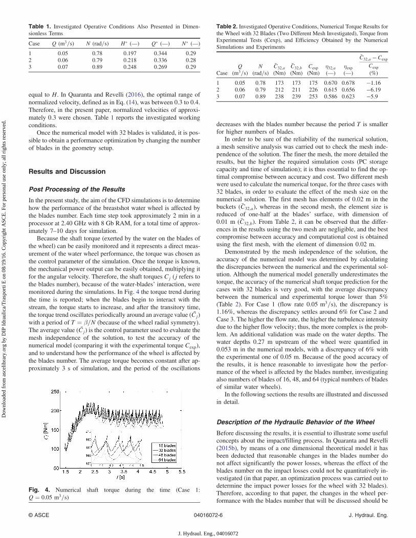
Because the shaft torque (exerted by the water on the blades ofthe wheel) can be easily monitored and it represents a direct meas-urement of the water wheel performance, the torque was chosen asthe control parameter of the simulation. Once the torque is known,the mechanical power output can be easily obtained, multiplying itfor the angular velocity. Therefore, the shaft torques Cj (j refers tothe blades number), because of the water-blades’ interaction, weremonitored during the simulations. In Fig. 4 the torque trend duringthe time is reported; when the blades begin to interact with thestream, the torque starts to increase, and after the transitory time,the torque trend oscillates periodically around an average value (Cj)with a period of T ¼ β=N (because of the wheel radial symmetry).The average value (Cj) is the control parameter used to evaluate themesh independence of the solution, to test the accuracy of thenumerical model (comparing it with the experimental torque Cexp),and to understand how the performance of the wheel is affected bythe blades number. The average torque becomes constant after ap-proximately 3 s of simulation, and the period of the oscillations

decreases with the blades number because the period T is smallerfor higher numbers of blades.

In order to be sure of the reliability of the numerical solution,a mesh sensitive analysis was carried out to check the mesh inde-pendence of the solution. The finer the mesh, the more detailed theresults, but the higher the required simulation costs (PC storagecapacity and time of simulation); it is thus essential to find the op-timal compromise between accuracy and cost. Two different meshwere used to calculate the numerical torque, for the three cases with32 blades, in order to evaluate the effect of the mesh size on thenumerical solution. The first mesh has elements of 0.02 m in thebuckets (C32;a), whereas in the second mesh, the element size isreduced of one-half at the blades’ surface, with dimension of0.01 m (C32;b). From Table 2, it can be observed that the differ-ences in the results using the two mesh are negligible, and the bestcompromise between accuracy and computational cost is obtainedusing the first mesh, with the element of dimension 0.02 m.

Demonstrated by the mesh independence of the solution, theaccuracy of the numerical model was determined by calculatingthe discrepancies between the numerical and the experimental sol-ution. Although the numerical model generally underestimates thetorque, the accuracy of the numerical shaft torque prediction for thecases with 32 blades is very good, with the average discrepancybetween the numerical and experimental torque lower than 5%(Table 2). For Case 1 (flow rate 0.05 m3=s), the discrepancy is1.16%, whereas the discrepancy settles around 6% for Case 2 andCase 3. The higher the flow rate, the higher the turbulence intensitydue to the higher flow velocity; thus, the more complex is the prob-lem. An additional validation was made on the water depths. Thewater depths 0.27 m upstream of the wheel were quantified in0.053 m in the numerical models, with a discrepancy of 6% withthe experimental one of 0.05 m. Because of the good accuracy ofthe results, it is hence reasonable to investigate how the perfor-mance of the wheel is affected by the blades number, investigatingalso numbers of blades of 16, 48, and 64 (typical numbers of bladesof similar water wheels).

In the following sections the results are illustrated and discussedin detail.

Description of the Hydraulic Behavior of the Wheel

Before discussing the results, it is essential to illustrate some usefulconcepts about the impact/filling process. In Quaranta and Revelli(2015b), by means of a one dimensional theoretical model it hasbeen deducted that reasonable changes in the blades number donot affect significantly the power losses, whereas the effect of theblades number on the impact losses could not be quantitatively in-vestigated (in that paper, an optimization process was carried out todetermine the impact power losses for the wheel with 32 blades).Therefore, according to that paper, the changes in the wheel per-formance with the blades number that will be discussed should be

Table 1. Investigated Operative Conditions Also Presented in Dimen-sionless Terms

Case Q (m3=s) N (rad=s) H� (—) Q� (—) N� (—)

1 0.05 0.78 0.197 0.344 0.292 0.06 0.79 0.218 0.336 0.283 0.07 0.89 0.248 0.269 0.29

Fig. 4. Numerical shaft torque during the time (Case 1:Q ¼ 0.05 m3=s)

Table 2. Investigated Operative Conditions, Numerical Torque Results forthe Wheel with 32 Blades (Two Different Mesh Investigated), Torque fromExperimental Tests (Cexp), and Efficiency Obtained by the NumericalSimulations and Experiments

CaseQ

(m3=s)N

(rad=s)C32;a(Nm)

C32;b(Nm)

Cexp(Nm)

η32;a(—)

ηexp(—)

C32;a − Cexp

Cexp

(%)

1 0.05 0.78 173 173 175 0.670 0.678 −1.162 0.06 0.79 212 211 226 0.615 0.656 −6.193 0.07 0.89 238 239 253 0.586 0.623 −5.9

© ASCE 04016072-6 J. Hydraul. Eng.

J. Hydraul. Eng., 04016072

Dow

nloa

ded

from

asc

elib

rary

.org

by

DIP

Idr

aulic

a/T

rasp

orti

E o

n 08

/19/

16. C

opyr

ight

ASC

E. F

or p

erso

nal u

se o

nly;

all

righ

ts r

eser

ved.

mainly attributed to the consequences on the impact and fillingprocess.

When the tip of the blade is coincident with the channel’s bedjust upstream of the wheel (Step 1), the impact configurations are intheir optimal conditions. In this situation, the stream flows alongthe blade without falling as a free jet and minimizing the impactpower losses (as long as the relative stream velocity is approxima-tively parallel to the blade inclination, as a correct design shouldprovide). If in Step 1 there are not other blades directly exposed tothe water stream (as an optimal design for this kind of breastshotwheels also should guarantee), the exerted impact torque on theconsidered blade in this configuration is not affected by the bladesnumber. While the blade rotates, the impact conditions begin tobecome more and more distant from the optimal ones; the relativeentry velocity moves away from the blade inclination, and the watermay also fall into the buckets as a free jet (Step 2). In this step, thebuckets are already partially filled; thus, the water flow impingesagainst a water volume (dissipating a portion of its kinetic energy),instead of performing useful work directly interacting with theblades. Hence, the impact power losses are very sensitive to theinstantaneous configuration, and they are significantly affectedby the wheel rotation.

Therefore, the temporal trend of the torque would experiencea peak value (Step 1) and after the peak, a decrease. When a newblade begins to interact with the flow, the impact torque increasesagain. As a consequence, the lower the blades number the longerthe decreasing part of the trend, and as a result, with the peakvalues reasonably coincident (because in the optimal configuration,Step 1, the kinetic energy of the flow transferred to the blade is notaffected by the blades number), the average torque decreases withthe decrease in the blades number. Moreover, the lower the bladesnumber, the bigger the water, which cumulates inside each bucketand interferes with the approaching water flow; thus, the higher thedissipation of the water kinetic energy.

The previous conjecture is confirmed observing Fig. 4. Consid-ering the numerical results for 32, 48, and 64 blades (as illustratedin the next paragraph), the monitored torque trend corresponds to

the expected trend described previously. The amplitude of the os-cillations decreases with the blades number and the peak values areclose together (the zoom reported in Fig. 4 clarifies the aspect, atthe temporal instant t ¼ 4.12 s). Instead, the torque correspondingto 16 blades is quite flat, and the peak of the torque is significantlylower. The qualitative and quantitative differences in the trend haveto be attributed to the different water behavior inside the filledbuckets, which now moves with pronounced oscillations.

Indeed, observing Fig. 5, the water surface in the buckets can beconsidered practically horizontal and at rest only in the range from32 to 64 blades, whereas in the case of 16 blades, the water insidethe buckets moves with bigger oscillations. This is a consequenceof the longer interaction between the entry stream and the watervolume already in the buckets because of the larger distance be-tween the blades (the water inside the buckets is also less confinedin the cases with 16 blades). Fig. 6 confirms what can be seen inFig. 5; in cases of 16 blades, the turbulent viscosity, as well as theturbulence intensity, is higher [μt ≃ 0.23 kg=ðm · sÞ at 16 bladesand μt ≃ 0.08 kg=ðm · sÞ at 64 blades] because a large amount ofkinetic energy of the entry flow causes an increase in the turbulenceof the water volume in the bucket, in spite of performing usefulwork on the blades. Therefore, in the range from 32 to 64 bladesit is reasonable to attribute the changes in the wheel performance(because of the different blades number) mainly to the blades num-ber effects on the impact and filling process, hence on the transferprocess of kinetic energy between the water flow and the blades.At 16 blades, additional power losses are also generated by thewater movements in the buckets and by the sooner release of waterinto the tailrace, situations that should be avoided.

Practical Results and Performance

As explained in the previous section, the torque was monitoredduring the time for each simulation, and the average value was usedas a main control parameter to evaluate the accuracy of the CFDmodel and to quantify the blades number effects on the perfor-mance of the wheel. The scope of the present section is to show

Fig. 5. Contour of volume fraction for Case 1: (a) 16; (b) 32; (c) 48; (d) 64 blades; white corresponds to the cells with only water present, and blackare those with only air; the transition between the two colors indicates the free surface and that the two fluids are mixed

© ASCE 04016072-7 J. Hydraul. Eng.

J. Hydraul. Eng., 04016072

Dow

nloa

ded

from

asc

elib

rary

.org

by

DIP

Idr

aulic

a/T

rasp

orti

E o

n 08

/19/

16. C

opyr

ight

ASC

E. F

or p

erso

nal u

se o

nly;

all

righ

ts r

eser

ved.

how the efficiency of the wheel is affected by the blades numberand to suggest some practical recommendations.

In Fig. 7 and Table 3, the shaft torque from numerical simula-tions is reported versus the blades number, whereas in Fig. 8 and

Table 4, the results are reported in terms of efficiency. The trendequation of the efficiency versus the blades number, which inter-polates the data in Fig. 8 and Table 4, is assumed to be

ηnum ¼ ayn2b þ bynb þ cy ð15Þ

where subscript y = each investigated case and

½a1; b1; c1� ¼ ½−3.7 · 10−5; 5.0 · 10−3; 0.55�;½a2; b2; c2� ¼ ½−6.0 · 10−5; 6.3 · 10−3; 0.49�;½a3; b3; c3� ¼ ½−5.7 · 10−5; 5.9 · 10−3; 0.45�

Eq. (15) is also reported in Fig. 8, where it can be observed thatthe number of blades affects the efficiency of the wheel. The maxi-mum increase in performance passing from 16 blades to the optimalblades number can be quantified between 12 and 16%, depending

Fig. 6. Contour of turbulent viscosity (kg=m · s) for Case 1: (a) 16 and (b) 64 blades

Fig. 7. Shaft torque from numerical simulations and experimental testsversus the blades number

Table 3. Investigated Operative Conditions, Numerical Torque Resultsfor the Wheel with 16, 32 (Two Different Mesh Investigated), 48, and64 Blades

CaseQ

(m3=s)N

(rad=s)C16

(Nm)C32;a(Nm)

C32;b(Nm)

C48

(Nm)C64

(Nm)C72

(Nm)

1 0.05 0.78 160 173 173 182 184 1852 0.06 0.79 199 212 211 229 224 —3 0.07 0.89 216 238 239 245 243 —

Note: Simulation for 72 blades was added for practical reasons to Case 1,as explained in the “Practical Results” section.

Fig. 8. Efficiency from numerical simulations versus the blades num-ber and trend equations

© ASCE 04016072-8 J. Hydraul. Eng.

J. Hydraul. Eng., 04016072

Dow

nloa

ded

from

asc

elib

rary

.org

by

DIP

Idr

aulic

a/T

rasp

orti

E o

n 08

/19/

16. C

opyr

ight

ASC

E. F

or p

erso

nal u

se o

nly;

all

righ

ts r

eser

ved.

on the flow rate. For Cases 2 and 3 (Q ¼ 0.06 and Q ¼0.07 m3=s, respectively) the optimal blades number among the in-vestigated ones is 48; after that, the efficiency starts to decrease.In Case 1 (Q ¼ 0.05 m3=s), the torque trend does not exhibit amaximum in the explored range. Therefore, an additional simula-tion was added for 72 blades to understand the performance forhigher numbers of blades (although 72 blades is not suggested forthis kind of wheel, for practical reasons).

Observing the trend lines in Fig. 8 for Cases 2 and 3, the theo-retical maximums are close to 48 blades, whereas for Case 1 themaximum is close to 64. This is a reasonable result because thehigher the flow rate, the bigger the buckets’ dimension can be.Because in Case 1 the performance practically does not changeafter 48 blades, nb ¼ 48 is suggested as the optimal blades numberfor this kind of breastshot water wheel.

Therefore, also in this work, an optimal blades number is iden-tified, as in the reference papers reported in the “Introduction” con-cerning stream water wheels. The achievement of optimal bladesnumbers is justified by the following practical motivations. Whenthe blades number is too small, only a few blades interact with thestream. When the water enters into the cells, the water flow loses ahigher amount of potential energy with respect to higher numbersof blades because the distance between two blades is larger.Furthermore, the jet dissipates a bigger amount of kinetic energy(see the previous section for further details), and the water will bethen released into the tailrace sooner. When the blades number istoo high, the space between two blades is too small to determineobstructions and additional power losses in the filling process; as aconsequence, the efficiency does not increase any more and gen-erally, the efficiency decreases.

Eq. (15) can be used as practical and simple tool to determineoptimal numbers of blades for geometrically similar breastshotwater wheels in similar working conditions. For these motivations,in order to make the results generically applicable, the hydraulicconditions are reported in Table 4 in dimensionless terms, whichare the dimensionless head and flow rate. It is also recommendedthat the optimal rotational wheel speed be included in the range0.3 < N� < 0.4 (Quaranta and Revelli 2016).

Although the present results illustrate that the number of bladesaffects the performance of the wheel, the blades number doesnot affect significantly the upstream and downstream conditions(Fig. 5). This means that it is possible to change the blades numberof similar breastshot water wheels without significant consequen-ces on the exploited channel.

Conclusion and Future Work

Although water wheels are a sustainable and efficient technology togenerate energy, only a small amount of research has been spent ontheir performance characteristics in the last century. They have beenanalyzed by several scientists in the eighteenth and early nineteenth

centuries, but the advent of modern turbines and electric motorsinterrupted the use of water wheels. In the last few years, the at-tention on water wheels has seen a revival, both from scientists andfrom some companies, which are currently manufacturing waterwheels for electricity generation. Water wheels are economicallyconvenient, environmentally friendly, and efficient hydropowerconverters for very low heads. Water wheels can therefore consti-tute an interesting investment both in industrialized countries and,in particular, in rural areas and the developing world.

In the present work, the effects of the blades number on the per-formance (thus on the power output and efficiency) of a breastshotwater wheel was reported, and the hydraulic behavior of the wheelwas investigated. In this paper, the range from 16 to 64 blades wasinvestigated. The results were carried out through numerical CFDanalyses for three hydraulic conditions (0.05, 0.06, and 0.07 m3=s,respectively); these conditions correspond to normalized head dif-ferences of H=D ¼ 0.197, H=D ¼ 0.218, and H=D ¼ 0.248 andnormalized flow rates of 0.344, 0.336, and 0.269, respectively.

The simulations show that the number of blades affects the per-formance of breastshot water wheels. The lower the blades number,the higher the loss of potential energy during the filling process andthe dissipation of the flow kinetic energy, the more significant thewater oscillations in the buckets and the sooner the release of waterdownstream. When the blades number is too high, the interferenceeffect on the entry water flow by the blades gives rise to powerlosses. The more the blades are, the more the volume that is sub-tracted from the buckets, and the maximum flow volume that canbe discharged may decrease. The maximum limit of the bladesnumber is also dictated by practical installation reasons. Therefore,the correct design of the number of the blades represents an impor-tant issue in water wheels design, particularly for breastshot wheelssimilar to the investigated one.

In the present case, the maximum increase in torque and effi-ciency from 16 blades to the optimal one is from 12 to 16%,depending on the flow rate. The optimal blades number can beestimated in 48 blades, which is the recommended prescriptionfor practical applications in similar working conditions. Eq. (15)can be used to estimate the effect of the blades number on the per-formance of similar breastshot water wheels.

For the future, CFD simulations will be used to investigate over-shot water wheels and the effect of the blades shape on breastshotwater wheels’ performance.

Acknowledgments

The research leading to these results has received funding fromORME (Energy optimization of traditional water wheels)—Granted by Regione Piemonte via the ERDF 2007–2013 (GrantNumber: #0186000275)—Partners Gatta srl, BCE srl, RigamontiGhisa srl, Promec Elettronica srl and Politecnico di Torino.

Notation

The following symbols are used in this paper:a = sluice gate opening;b = wheel width;

Cexp = experimental torque;Cj = numerical torque for blades number j;D = wheel diameter;g = gravitational acceleration;H = energy head;H� = normalized energy head;I = turbulent intensity;

Table 4. Investigated Operative Conditions in Dimensionless Terms andEfficiency for the Wheel with 16, 32, 48, and 64 Blades

CaseHD

N · Rffiffiffiffiffiffiffiffiffi2gH

p QðN · RÞH2 η16 η32;a η48 η64 η72

1 0.197 0.29 0.344 0.62 0.67 0.70 0.71 0.722 0.218 0.28 0.336 0.58 0.62 0.67 0.65 —3 0.248 0.29 0.269 0.53 0.58 0.60 0.59 —

Note: R is the wheel radius; for Case 1, 72 blades were also investigated forpractical reasons, as explained in the “Practical Results” section.

© ASCE 04016072-9 J. Hydraul. Eng.

J. Hydraul. Eng., 04016072

Dow

nloa

ded

from

asc

elib

rary

.org

by

DIP

Idr

aulic

a/T

rasp

orti

E o

n 08

/19/

16. C

opyr

ight

ASC

E. F

or p

erso

nal u

se o

nly;

all

righ

ts r

eser

ved.

k = turbulence kinetic energy;N = wheel rotational speed;N� = normalized wheel rotational speed;nb = blades number;

Pexp = experimental power output;Pin = power input;p = time averaged pressure;Q = flow rate;Q� = normalized flow rate;R = wheel radius;T = period of torque oscillations;t = time;ui = time averaged flow velocity in direction xi;u 0i = velocity fluctuation in direction xi;

xi, xj, xw = orthogonal components of the reference system;αq = volume fraction of phase q;β = angular distance between two blades;ϵ = turbulent dissipation;η = efficiency;μ = dynamic viscosity of the mixture;μt = dynamic turbulent viscosity;ρ = density;τ = tangential turbulent stress; andω = specific dissipation rate.

References

Akinyemi, O. S., and Liu, Y. (2015a). “CFD modeling and simulationof a hydropower system in generating clean electricity from water flow.”Int. J. Energy Environ. Eng., 6(4), 357–366.

Akinyemi, O. S., and Liu, Y. (2015b). “Evaluation of the power generationcapacity of hydrokinetic generator device using computational analysisand hydrodynamics similitude.” J. Power Energy Eng., 3(8), 71–82.

Bach, C. (1886). Die Wasserräder: Atlas (The water wheels: Technicaldrawings), Konrad Wittwer Verlag, Stuttgart, Germany (in German).

Barstad, L. F. (2012). “CFD analysis of a pelton turbine.” M.Sc. thesis,Norwegian Univ. of Science and Technology, NTNU, Trondheim,Norway.

Bodis, K., Monforti, F., and Szabo, S. (2014). “Could Europe havemore mini hydro sites? A suitability analysis based on continentallyharmonized geographical and hydrological data.” Renewable Sustain-able Energy Rev., 37, 794–808.

Bozhinova, S., Kisliakov, D., Müller, G., Hecht, V., and Schneider, S.(2013). “Hydropower converters with head differences below 2.5 m.”Proc. ICE-Energy, 166(3), 107–119.

Capecchi, D. (2013). “Over and undershot waterwheels in the 18th century.Science-technology controversy.” Adv. Historical Stud., 2(3), 131–139.

Chaudy, F. (1896). “Machines hydrauliques.” Bibliothèque du conducteurde travaux publics, Vve. C. Dunod et P. Vicq (in French), Sablonse,France.

Church, I. P. (1914). Hydraulic motors, with related subjects, includingcentrifugal pumps, pipes, and open channels, designed as a text-bookfor engineering schools, Wiley, London.

ESHA (European Small Hydropower Association). (2014). Small andmicro hydropower restoration handbook, National Technical Univ.of Athens, Athens, Greece.

Garuffa, E. (1897). “Macchine motrici ed operatrici a fluido.” Meccanicaindustrial, Univ. of California, Oakland, CA (in Italian).

Gotoh, M., Kowata, H., Okuyama, T., and Katayama, S. (2001). “Charac-teristics of a current water wheel set in a rectangular channel.” Proc.,ASME Fluids Engineering Division Summer Meeting, Vol. 2, ASME,New York, 707–712.

Liu, Y. C., and Peymani, F. Y. (2015). “Development and computationalverification of an analytical model to evaluate performance of paddlewheel in generating electricity from moving fluid.” Distrib. Gener.Altern. Energy J., 30(1), 58–80.

Luther, S., Wardana, I. N. G., Soenoko, R., and Wahyudi, S. (2013).“Performance of a straight-bladed water-current turbine.” Adv. Nat.Appl. Sci., 7(5), 455–461.

Menter, F. (1994). “Two-equation eddy-viscosity turbulence models forengineering applications.” AIAA J., 32(8), 1598–1605.

Morin, A., and Morris, E. (1843). Experiments on water wheels having avertical axis, called turbines, Franklin Institute, Metz, Paris.

Müller, G., Denchfield, S., Marth, R., and Shelmerdine, R. (2007). “Streamwheels for applications in shallow and deep water.” Proc., 32nd IAHRCongress, IAHR, Venice, Vol. 32, 707–716.

Müller, G., Jenkins, R., and Batten, W. M. J. (2010). Potential,performance limits and environmental effects of floating water mills,A. Dittrich, Ka. Koll, J. Aberle, and P. Geisenhainer, eds., Univ. ofSouthampton, Highfield, U.K.

Müller, G., and Kauppert, K. (2004). “Performance characteristics of waterwheels.” J. Hydraul. Res., 42(5), 451–460.

Olsson, E., Kreiss, G., and Zahedi, S. (2007). “A conservative levelset method for two phase flow II.” J. Comput. Phys., 225(1),785–807.

Osher, S., and Sethian, J. A. (1988). “Fronts propagating with curvature-dependent speed: Algorithms based on Hamilton-Jacobi formulations.”J. Comput. Phys., 79(1), 12–49.

Poncelet, J. V. (1843). Memoria sulle ruote idrauliche a pale curve, mossedi sotto, seguita da sperienze sugli effetti meccanici di tali ruote,E. Dombré, ed., Dalla tipografia Flautina, Napoli, Italy.

Pujol, T., Solà, J., Montoro, L., and Pelegrí, M. (2010). “Hydraulic perfor-mance of an ancient Spanish watermill.” Renewable Energy, 35(2),387–396.

Quaranta, E., and Müller, G. (2016). “Zuppinger and Sagebien waterwheels for very low head applications.” J. Hydraul. Res., in press.

Quaranta, E., and Revelli, R. (2015a). “Output power and power lossesestimation for an overshot water wheel.” Renewable Energy, 83,979–987.

Quaranta, E., and Revelli, R. (2015b). “Performance characteristics, powerlosses and mechanical power estimation for a breastshot water wheel.”Energy, 87, 315–325.

Quaranta, E., and Revelli, R. (2016). “Optimization of breastshot waterwheels performance using different inflow configurations.” RenewableEnergy, 97, 243–251.

Tevata, A., and Chainarong, I. (2011). “The effect of paddle number andimmersed radius ratio on water wheel performance.” Energy Procedia,9, 359–365.

Vidali, C., Fontan, S., Quaranta, E., Cavagnero, P., and Revelli, R. (2016).“Experimental and dimensional analysis of a breastshot water wheel.”J. Hydraul. Res., 54(4), 473–479.

Weisbach, J. (1849). Principles of the mechanics of machinery andengineering, Lea & Blanchard, PA.

© ASCE 04016072-10 J. Hydraul. Eng.

J. Hydraul. Eng., 04016072

Dow

nloa

ded

from

asc

elib

rary

.org

by

DIP

Idr

aulic

a/T

rasp

orti

E o

n 08

/19/

16. C

opyr

ight

ASC

E. F

or p

erso

nal u

se o

nly;

all

righ

ts r

eser

ved.