hybridization of particle swarm optimization with …
TRANSCRIPT

HYBRIDIZATION OF PARTICLE SWARM OPTIMIZATION WITH BAT ALGORITHM FOR OPTIMAL REACTIVE POWER DISPATCH
by
EMMANUEL EMENIKE AGBUGBA
submitted in accordance with the requirements for the degree of
MAGISTER TECHNOLOGIAE
In the subject
ELECTRICAL ENGINEERING
at the
University of South Africa
Supervisor: Prof. Zenghui Wang
June 2017

ii
DECLARATION
Name: EMMANUEL EMENIKE AGBUGBA Student number: 57441022 Degree: MAGISTER TECHNOLOGIAE Exact wording of the title of the dissertation or thesis as appearing on the copies submitted for examination:
HYBRIDIZATION OF PARTICLE SWARM OPTIMIZATION WITH BAT ALGORITHM FOR
OPTIMAL REACTIVE POWER DISPATCH
I declare that the above dissertation/thesis is my own work and that all the sources that I have
used or quoted have been indicated and acknowledged by means of complete references.
13 – 06 - 2017 ________________________ _____________________ SIGNATURE DATE

iii
This dissertation is dedicated to my loving wife Loveth Mmirmma Agbugba

iv
ACKNOWLEDGEMENT
I would like to thank my supervisor Professor Zenghui Wang, Department of Electrical and Mining
Engineering for his constant motivation and support during the course of my dissertation. I am
thankful for his valued tutelage and support all through the period of my study. I am highly
indebted to him for being patient with me. I was honoured to have him as my supervisor.
I owe all to my wife Loveth and children Emmanuel (Jnr.), Grace and Joshua. Without their
unconditional love and support I would not have reached this height and dream.
I owe a debt of gratitude to my mother Comfort Ejindu Agbugba for her love and prayers.
I am eternally grateful to my brothers Francis, Anthony and Michael; and my sisters Mary and
Catherine for their support, understanding and constant encouragement.

v
ABSTRACT
This research presents a Hybrid Particle Swarm Optimization with Bat Algorithm (HPSOBA) based
approach to solve Optimal Reactive Power Dispatch (ORPD) problem. The primary objective of
this project is minimization of the active power transmission losses by optimally setting the control
variables within their limits and at the same time making sure that the equality and inequality
constraints are not violated. Particle Swarm Optimization (PSO) and Bat Algorithm (BA)
algorithms which are nature-inspired algorithms have become potential options to solving very
difficult optimization problems like ORPD. Although PSO requires high computational time, it
converges quickly; while BA requires less computational time and has the ability of switching
automatically from exploration to exploitation when the optimality is imminent. This research
integrated the respective advantages of PSO and BA algorithms to form a hybrid tool denoted as
HPSOBA algorithm. HPSOBA combines the fast convergence ability of PSO with the less
computation time ability of BA algorithm to get a better optimal solution by incorporating the BA’s
frequency into the PSO velocity equation in order to control the pace. The HPSOBA, PSO and BA
algorithms were implemented using MATLAB programming language and tested on three (3)
benchmark test functions (Griewank, Rastrigin and Schwefel) and on IEEE 30- and 118-bus test
systems to solve for ORPD without DG unit. A modified IEEE 30-bus test system was further used
to validate the proposed hybrid algorithm to solve for optimal placement of DG unit for active
power transmission line loss minimization. By comparison, HPSOBA algorithm results proved to
be superior to those of the PSO and BA methods.
In order to check if there will be a further improvement on the performance of the HPSOBA, the
HPSOBA was further modified by embedding three new modifications to form a modified Hybrid
approach denoted as MHPSOBA. This MHPSOBA was validated using IEEE 30-bus test system to
solve ORPD problem and the results show that the HPSOBA algorithm outperforms the modified
version (MHPSOBA).
Keywords—Hybridization; Hybrid Particle Swarm Optimization (HPSOBA); Modified Hybrid
Particle Swarm Optimization (MHPSOBA); Optimal Power Flow (OPF); Optimal Reactive Power
Dispatch (ORPD); Particle Swarm Optimization (PSO); Bat Algorithm (BA); Active Power Loss
Minimization; Benchmark Functions; Distributed Generation (DG); Conventional Optimization
Technique; Evolutionary Optimization Technique; Artificial Intelligence; Equality Constraints;
Inequality Constraints; Penalty Function.

vi
TABLE OF CONTENTS
Declaration ii
Dedication iii
Acknowledgement iv
Abstract v
Table of Contents vi
List of Tables ix
List of Figures x
Acronyms and Abbreviations xi
Chapter 1: Introduction 1
1.1 Research Background 1
1.2 Motivation 3
1.3 Objectives 4
1.4 Research Questions 4
1.5 Scope of the Research 5
1.6 Outline of the Disssertation 5
Chapter 2: Literature Review 7
2.1 Optimal Reactive Power Dispatch 7
2.1.1 Conventional Optimization Techniques 8
2.1.2 Evolutionary Optimization Techniques 10
2.2 The ORPD Problem Formulation 13
2.2.1 Equality Constraints 14
2.2.2 Inequality Constraints 14
2.2.3 Penalty Function 15
2.3 Particle Swarm Optimization 16
2.3.1 PSO Algorithm Pseudo Code 19
2.3.2 Basic Fundamentals of The PSO 22
2.4 Bat Algorithm 24
2.4.1 Movements of Virtual Bats 25

vii
2.4.2 Loudness and Pulse Emission 26
2.4.3 Bat Algorithm Pseudo code 27
2.5 Hybridization of Evolutionary Algorithms to solve ORPD 30
2.6 Optimal Placement of DG Unit(s) 33
2.7 Summary 34
Chapter 3: Hybrid PSO-BA Model 35
3.1 Motivation for Hybridization of PSO with BA 35
3.2 Proposed Hybrid PSO-BA (HPSOBA) Methodology 36
3.3 Test Function Optimization using HPSOBA 39
3.3.1 Simulation Results and Analysis of Test Function
Optimization 39
3.4 Solving ORPD Problem Using HPSOBA 41
3.4.1 Case I: Simulation Results and Analylsis of Solving
ORPD Without A DG Unit 41
3.4.1.1 IEEE 30-Bus Test System 42
3.4.1.2 IEEE 118-Bus Test System 46
3.4.2 Case II: Optimal placement of A DG unit Using HPSOBA 51
3.4.2.1 Simulation Results and Analylsis of
Solving ORPD With A DG Unit 51
3.5 Summary 57
Chapter 4: Modified HPSOBA 58
4.1 Overview 58
4.2 Modifications of HPSOBA Algorithm 58
4.2.1 1st Modification (Pulse Frequency) 58
4.2.2 2nd Modification (Velocity Vector) 59
4.2.3 3rd Modification (Pulse rate and Loudness Update) 59
4.3 Simulation Results and Analysis of Solving ORPD Using

viii
MHPSOBA 60
4.4 Summary 61
Chapter 5: Conclusion and Future Work 62
5.1 Conclusion 62
5.2 Future Work 64
List of Publications 65
References 66
Appendices 77
Appendix A: Standard IEEE 30- and 118-Bus Test Systems Data
Appendix A.1 Standard IEEE 30-Bus Test System Data 77
Appendix A.2 Standard IEEE 118-Bus Test System Data 78
Appendix B: Sample Codes for Algorithms of ORPD
(IEEE 30-Bus Test System)
Appendix B.1 MATLAB codes for PSO Algorithm for ORPD 85
Appendix B.2 MATLAB codes For BA Algorithm for ORPD 89
Appendix B.3 MATLAB codes for HPSOBA Algorithm
for ORPD 93
Appendix C: Sample Codes for Algorithms of ORPD
(IEEE 118-Bus Test System)
Appendix C.1 MATLAB codes for PSO Algorithm for ORPD 98
Appendix C.2 MATLAB codes For BA Algorithm for ORPD 108
Appendix C.3 MATLAB codes for HPSOBA Algorithm
for ORPD 118

ix
LIST OF TABLES
Table Page
I. Comparison between different algorithms on 3 standard
benchmark functions 40
II. Parameters and data settings for the proposed algorithms 41
III. IEEE 30-bus test system control variables limits for ORPD 43
IV. Comparative results of IEEE 30-bus test system 45
V. Values of control variables before and after optimization
for IEEE 30-bus test system 45
VI. IEEE 118-bus test system control variables limits for ORPD 47
VII. Comparative results of IEEE 118-bus test system 49
VIII. Values of control variables before and after optimization
for IEEE 118-bus test system 49
IX. Modified IEEE 30-bus test system constraints for DG Unit
Optimal Installation 52
X. Comparative results of the DG Unit placement on each bus 52
XI. Comparative results of HPSOBA Algorithm for with and
without DG Unit placement 54
XII. Values of control variables before and after optimal placement of DG Unit
for modified IEEE 30-bus test system 55
XIII. Comparative results of MHPSOBA algorithm with HPSOBA
for solving ORPD problem 60
XIV. Comparative values of control variables after optimization for HPSOBA and
MHPSOBA methods for IEEE 30-bus test system 61
XV. Algorithm performance summary for solving ORPD problem 63

x
LIST OF FIGURES
Figure Page
1. Conventional PSO Flowchart 20
2. Conventional BA Flowchart 29
3. Proposed HPSOBA Flowchart 38
4. Single-line diagram of IEEE 30-bus test system 42
5. Average convergence curve of PSO for IEEE 30-bus test system 43
6. Average convergence curve of BA for IEEE 30-bus test system 44
7. Average convergence curve of HPSOBA for IEEE 30-bus test system 44
8. Single-line diagram of IEEE 118-bus test system 46
9. Average convergence curve of PSO for IEEE 118-bus test system 47
10. Average convergence curve of BA for IEEE 118-bus test system 48
11. Average convergence curve of HPSOBA for IEEE118-bus test system 48
12. Graph of the comparative results of the DG unit placement on each bus 53
13. Average convergence curve of HPSOBA for modified 30-bus test system 54
xi
ACRONYMS AND ABBREVIATIONS
ABC Artificial Bee Colony
ACO Ant Colony Optimization
AGA Adaptive Genetic Algorithm
ALC Aging Leader and Challengers
BA Bat Algorithm
BFO Bacterial Foraging Optimization
BHBO Black Hole Based Optimization
CA Coordinated Aggregation
CLPSO Comprehensive Learning Particle Swarm
Optimization
CS Cuckoo Search
CSO Cat Swarm Optimization
CSO Competitive Swarm Optimizer
DDE Double Differential Evolution
DE Differential Evolution
DG Distributed Generation
DLP Dual Linear Programming
DSA Differential Search Algorithm
EP Evolutionary Programming
FA Firefly Algorithm
GA Genetic Algorithm
GPAC General Passive Congregation
GPM Gradient Projection Method
GSA Gravitational Search Algorithm
GWO Gray Wolf Optimizer
HAS Harmony Search Algorithm
HBA Hybrid BA
HBO Honey Bees Optimization
HPSOBA Hybrid Particle Swarm Optimization with Bat
Algorithm
HPSOM Hybrid Particle Swarm Optimization with Mutation
IBA Improved Bat Algorithm
ICA Imperialist Competitive Algorithm

xii
IEEE Institute of Electrical and Electronics Engineers
IEP Improved Evolutionary Programming
IGA Improved Genetic Algorithm
IHSA Improved Harmony Search Algorithm
IP Interior Point
IPM Interior Point Method
IWO Invasive Weed Optimization
LP Linear Programming
LPAC Local Passive Congregation
MAPSO Multi-Agent PSO
MAS Multi-Agent System
MHPSOBA Modified Hybrid Particle Swarm Optimization with
Bat Algorithm
MICA Modified Imperialist Competitive Algorithm
MTLA Modified Teaching Learning Algorithm
MW Mega Watts
NM Nelder Mead
OGSA Opposition Based Gravitational Search Algorithm
OPF Optimal Power Flow
ORPD Optimal Reactive Power Dispatch
PCSO Parallel Cat Swarm Optimization Algorithm
PL Active Power Transmission Loss
PSO Particle Swarm Optimization
PSO-TVAC PSO with Time Varying Acceleration Coefficients
QIPM Quadratic Interior Point Method
QOBL Quasi-Opposition Based Learning
QP Quadratic Programming
QPSO Quantum Behaved PSO
s Seconds
SOA Seeker Optimization Algorithm
SQP Sequential Quadratic Programming
TCSC Thyristor Controlled Series Capacitor
TLBO Teaching Learning Based Optimization
TS Tabu Search
UPFC Unified Power Flow Controller

xiii
VAR Volt Amperes Reactive
VSL Voltage Stability Limit

1
CHAPTER 1
INTRODUCTION
1.1 RESEARCH BACKGROUND
Electric power systems are comprised of large and complex components that produce electrical
energy. A modern electric power system has the following components: 1) generating power plants,
2) transmission lines, 3) distribution lines, and 4) loads. The long transmission lines carry the
generated electric power from the generating stations to the loads. Every power system has the
primary objective of supplying cheap, reliable and optimized power to the consumers. In the bid to
optimize the power supplied to the various loads, the system encounters problems which are
summarily referred to as Power System Optimization problems.
Optimization problems, which are widely encountered in electric power systems, can be very
complex and non-linear depending on the nature of the fitness function. The goal of an optimization
problem can be stated thus: finding the amalgamation of control or decision variables that optimize
a given objective function to be maximized or minimized, possibly subject to some constraints on
the allowed parameter values. Generally, the classifications of the optimization problems are done
according to the mathematical features of the fitness function, constraints and control variables. The
problem formulation of any optimization problem can be thought of as a sequence of steps [1].
These steps are:
1) Choosing the design variables (control and state variables)
2) Formulating constraints
3) Formulating objective functions
4) Setting up variable limits
5) Choosing an optimization technique to solve the problem
6) Solving the problem in order to obtain the optimal solution.
In recent years, the electric power industry has experienced a major turn-around in the form of
deregulation or restructuring. Deregulation is all about of removing or reducing government
monopolistic control over prices with the introduction of independent power providers thereby
giving consumers the power to choose their utility providers [2]. This led to competitive market in
the power industry which results in lowering of electricity prices, innovation and expansion of the
power industry. This competitive market reduces cost but unarguably bring uncertainty to
generation forecasting as power producers compete to sell electricity. Meanwhile, in most places,
2
the rate of energy consumption has outpaced infrastructure development, placing pressure on the
aging equipment. These factors contribute to the increasing need for fast and reliable optimization
methods that can address both security and economic issues simultaneously in support of power
system operation and control [3].
One of the most significant optimization problems in electric power systems is Optimal Power Flow
(OPF) which was introduced by Carpentier [4] in 1962, and since then there has been a tremendous
development and algorithmic improvement. The primary objective of OPF is to obtain the optimal
state of the control variables by minimizing an objective function for a particular power system
while keeping all constraints (equality and inequality constraints) within limits [5]. Optimal
Reactive Power Dispatch (ORPD) is a sub-problem of the OPF problem, which determines all kinds
of controllable variables for optimal operation. In an ORPD, the values of some (or all) of the
control variables need to be found so as to optimize (maximize or minimize) a predefined objective
function. It is also important that the proper problem definition with clearly stated objective be
given at the onset. The most common ORPD objective functions are minimization of active power
transmission loss, minimization of generation cost, maximization of power quality (often by
minimizing voltage deviation) and minimization of capital cost during system planning [6]. The
active power transmission line loss leads to power shortages which affects the economic growth of
a country. For reliable operation of any power system, the power transmission losses are to be
minimized. This objective can be accomplished by optimizing the control variables such as
generator bus voltages (continuous variable), transformer tap ratio or position, and reactive power
output of shunt compensations (discrete variables) [7].
The ORPD problem is a non-continuous and non-linear objective function optimization problem
which requires a more complex formulation, as the set of equations involved may not be linearized.
Solving ORPD problems has the advantage of, but not limited to, minimization of active power
transmission loss and power factor improvement in the distribution system. The ORPD problem can
also be described as a complex and combinatorial optimization problem which contains both
continuous and discrete control variables [8]. In this case, non-linear optimization
methods/techniques must be employed. There are two optimization methods used in solving ORPD
optimization problems namely Conventional and Evolutionary/Artificial Intelligence Optimization
Techniques. A number of conventional techniques such as Newton-Raphson Method [9], Quadratic
Programming (QP) [10, 11], Interior Point Method (IPM) [12, 13] and Linear Programming (LP)
[14, 15] have been successfully applied to solving the ORPD problem. Traditional optimization
methods which use gradients for the search of the optimum, need a function that is at least twice
3
differentiable and are inefficient in dealing with discrete variables-based problems which results in
their incapability for solving ORPD problems [16]. In the past, some evolutionary methods have
been applied to solve the ORPD problems in a bid to surmount the disadvantages imposed by the
conventional methods. Such evolutionary methods include Evolutionary Programming (EP) [17],
Genetic Algorithm (GA) [18, 19], Bat Algorithm (BA) [20], Seeker Optimization Algorithm (SOA)
[21], Differential Evolution (DE) [22–24], Bacterial Foraging Optimization (BFO) [25], Differential
Evolution (DE) [26] and Particle Swarm Optimization (PSO) [27]. Thus, evolutionary optimization
techniques have become an alternative to traditional optimization techniques for solving ORPD
problems since real-world problems are non-convex, non-differentiable and discontinuous.
1.2 MOTIVATION
The electric power system conveys bulk electrical energy from the generating plants to the
consumers via power substations, while sustaining tolerable or standardized power and voltage
qualities and limits for all consumers. The electrical energy from the generating station is delivered
to the consumer terminals through transmission and distribution networks. The generating stations
supply both active power and reactive power to the consumers. The consumer terminals need a
substantially constant voltage for satisfactory operation, but in practice, electric loads are time
variant which means that the consumer loads change over time causing power and current
fluctuations. On no-load conditions, the reactive power is required for magnetizing purposes while
on load conditions, the reactive power requirement depends on the nature of the load which can be
real, reactive or both.
Reactive power requirement changes continuously with load and system configuration. The change
in reactive power causes voltage variations in the system. Any change in the system formation or in
power demands may results in the change of voltage levels in the system. Injecting reactive power
into the power system raises voltages while absorbing the reactive power from the system lowers
voltages. The main task of a power system is to sustain the load bus voltages within the nominal
range for consumer satisfaction especially in a deregulated or restructured power industry. Despite
the importance of deregulation which includes but is not limited to removal or reduction of
government control over the power industry and electricity price reduction etc., it leads to
expansion and reconfiguration of the power system. This situation, if not properly handled, can lead
to huge active power transmission line losses. These power transmission losses lead to power
shortage, voltage collapse and electrical blackouts which affects the economic growth of the
country. For reliable operation of any power system, the active power transmission losses are to be
minimized. This situation can be improved by the operator through reallocation of reactive power

4
generation in the system by modelling it as an ORPD optimization problem (without and without a
DG unit optimally installed) with the active power transmission loss as the objective function.
1.3 OBJECTIVES
The following are some of the objectives of this research:
1) To explore the advantages and disadvantages of PSO and BA optimization techniques.
2) To explore the applications of the PSO and BA optimization techniques in solving the
ORPD problems (with and without a DG unit).
3) To design a hybrid method of PSO with BA optimization techniques in order to extend the
PSO capabilities and improve its accuracy in solving ORPD problems (with and without a
DG unit).
4) To demonstrate the application and implementation of the hybridized PSO-BA algorithm in
solving ORPD problems (with and without a DG unit) for active power transmission loss
minimization.
5) To investigate the effects of BA’s frequency (f1) or two frequencies (f1and f2) on the PSO
algorithm’s velocity update equation.
6) To investigate the effect of optimal placement of a DG unit in solving an ORPD problem
using the hybrid approach.
7) To compare the results from the above and draw conclusion.
1.4 RESEARCH QUESTIONS
The major question this project tends to answer is:
“How can a standard PSO be hybridized with a BA algorithm to solve an ORPD problem for an
Active Power Transmission Loss Minimization Objective Function?”
In the quest to finding an answer to the above research question, the following sub-questions need
to be answered as well:
Q1) What are the advantages and disadvantages of the PSO algorithm and BA algorithm?
Q2) Can the drawbacks of premature convergence of a PSO algorithm be avoided by
hybridization with a BA algorithm?
Q3) Is it possible to combine PSO and BA algorithms to solve ORPD problem?
Q4) If Q3 is possible, how then can the combination be achieved?
Q5) What are the effects of the BA’s frequency (f1) or two frequencies (f1and f2) on the PSO
algorithm’s velocity update equation?
5
Q6) What is the effect of removing randomness from the PSO algorithm’s velocity and
position vectors thereby allowing pbest and gbest to govern the update during iteration
in the hybrid approach?
Q7) What are the effects of monotonically increasing and decreasing the pulse rate and
loudness respectively during the hybrid approach iterative update?
Q8) How can the equality and inequality constraints of the ORPD problem be restricted
without violation?
Q9) Where necessary, what kind of penalty function is imposed?
Q10) What can be done to further reduce the active power transmission line losses?
Q11) How can a distributed generation unit be optimally placed in a distribution network?
Q12) What is the effect of optimal placement of a DG unit in solving an ORPD problem using
a PSO-BA hybrid approach?
1.5 SCOPE OF THE RESEARCH
The research is limited to form a hybrid algorithm by combining PSO with BA for solving an
ORPD problem (denoted as HPSOBA). The research is also limited to investigating only the active
power transmission loss objective function and validation by using standard benchmark test
functions (Griewank, Rastrigin and Schwefel) and on IEEE 30- and 118-bus test systems to solve
for an ORPD problem without a DG unit on a MATLAB programming platform. A modified IEEE
30-bus test system was further used to validate the proposed algorithm to solve for optimal
placement of a DG unit for active power transmission line loss minimization. The equality and
inequality constraints are also taken into consideration and where necessary a penalty function is
imposed when constraints are violated.
A further modification of the HPSOBA algorithm was also considered to check if there will an
improvement of the hybrid approach performance in solving for ORPD problem or not.
1.6 OUTLINE OF THE DISSERTATION
The organization of the thesis is as follows:
Chapter 1, “Introduction” presents the research background, motivation, objectives, research
questions, scope and outline of this dissertation.
Chapter 2, “Literature Review” surveys the methods applied in solving the ORPD problem in the
past and the current scenario are presented considering the PSO and BA methods. The ORPD is
also presented alongside its problem formulation and objective functions. The ORPD problem

6
formulation consists of equality (power flow) and inequality (control variables) constraints. The
restriction of state variables is done by adding them as quadratic penalty terms to the objective
function. It also describes the PSO and BA pseudo code and their basic fundamentals.Also
presented in this chapter is the review and application of optimal placement of DG unit(s) to solving
an ORPD problem.
Chapter 3, “Hybrid PSO-BA Model” describes the hybridization of the PSO with the BA algorithm
including its motivations. The approach was carefully designed to achieve a better and quality
optimized result. Standard benchmark test functions and IEEE 30- and IEEE 118-bus test systems
were used to validate the robustness, accuracy and efficiency of the proposed approach. The
simulation results and analysis of the test function optimization and ORPD problem were presented
and compared with other results in the literature. A modified IEEE 30-bus test system was further
used to validate the proposed algorithm to solve for optimal placement of DG unit for active power
transmission line loss minimization.
Chapter 4, “Modified HPSOBA” The hybrid approach (HPSOBA) proposed by this research was
further modified to form a modified hybrid approach denoted as MHPSOBA by embedding three
new modifications. IEEE 30-bus test system was used to validate this approach to solve for the
ORPD problem. The evaluated results were compared with the base case and HPSOBA methods.
Chapter 5, “Conclusion” summarizes the outcomes of the research and outlines the contributions
of this research to the development of power systems.

7
CHAPTER 2
LITERATURE REVIEW
This chapter reviews the ORPD problem as part of optimization problems encountered in electric
power systems and some of the optimization techniques applied in solving the ORPD problem. A
brief discussion of both conventional and evolutionary techniques is presented. PSO, BA and
hybridization of evolutionary techniques to solving ORPD problem are also reviewed as well as the
optimal placement of the DG unit(s) in the distribution networks to reduce active power
transmission line losses. This chapter also covers the ORPD problem formulation, the constraints
(both equality and inequality) to which the objective function is subjected to are also defined here.
2.1 OPTIMAL REACTIVE POWER DISPATCH
The difficulty of solving ORPD problems increases significantly with increasing network size and
complexity. Recent industry developments have greatly increased electric power system
complexity. In prior decades, utilities had relatively few generators compared to the numbers
introduced today by the advent of independent power producers. Meanwhile, demand response
programs add variables to the load side of ORPD problems. Unfortunately, these developments
have discouraged the use of ORPD in many real-world applications [28, 29]. However, many
ORPD solution methods have been developed, each with distinct mathematical characteristics and
computational requirements. ORPD solutions methods vary considerably in their adaptability to the
modelling and solution requirements of different power system applications.
ORPD optimization problem formulations differ greatly depending on the particular selection of
variables, objective(s) and constraints. Because of the specialized nature of ORPD, the formulation
selection often has implications for both solution method design and solution accuracy. The two
major types are Conventional and Evolutionary optimization techniques.
Traditionally, conventional methods are effectively used to solve ORPD problems. They have been
applied to solving ORPD problems to suit the different objective functions and constraints. These
techniques are based on mathematical formulations which have to be simplified in order to get an
optimal solution. Some of the weakness of the conventional methods include: limited ability in
solving real-world large scale optimization problems, weakness in handling constraints, poor
convergence and stagnation, slow computational time (especially if the number of variables are
large) and expensive in computing large power system solutions [30].

8
To overcome the shortcomings of conventional techniques, evolutionary methods and their
hybridized versions have been developed and applied to ORPD problems in the recent past. The
major advantages of the evolutionary methods include: fast convergence rate, appropriate for
solving non-linear optimization problems, ability to find global optimum solutions, suitable for
solving multi-objective optimization problems, pertinent in finding multiple optimal solutions in a
single simulation run and versatile in handling constraints [31].
2.1.1 CONVENTIONAL OPTIMIZATION TECHNIQUES
The development of conventional optimization techniques and their applications to solve ORPD
problems are briefed here.
In reference [32], Mamundur and Chenoweth used Dual Linear Programming (DLP) to determine
the optimal settings of the ORPD control variables simultaneously satisfying the constraints. The
method employs linearized sensitivity relationships of power systems to establish both the objective
function for minimizing the active power transmission line losses and the system performance
sensitivities relating dependent and control variables. This technique is particularly suitable to
minimize system losses under operating conditions.
Reference [33]used P-Q decomposition approach to formulate OPF based upon the decoupling
principle well recognized in bulk power transmission load flow. This approach decomposes the
OPF formulation into a P-problem (real power model) and Q-problem (reactive power model),
thereby showing ORPD as a sub-problem of OPF. The Q-Problem is defined as the minimization of
real power transmission line losses by optimally setting the generator voltages, transformer tap
settings and shunt reactive power compensations. The problem of enforcing state variables
(inequality constraints) is included in the problem formulation by use of penalty functions. This
approach simplifies the formulation, improves computation time and permits certain flexibility in
the types of calculations desired (i.e. P-Problem, Q-Problem or both).
Burchett et al. [34] in their paper proposed a Quadratic Programming (QP) solution to the OPF
problem. This method used the second derivatives of the objective function to find the optimal
solution. This method is suitable for optimization problems with infeasible or divergent starting
points.
Lee et al. [35] broadly solved the OPF problem by decomposing the problem into P-optimization
module and Q-optimization module and solved them using the Gradient Projection Method (GPM)

9
for the first time in a power system optimization study. This GPM technique allows the use of
functional constraints without the need of penalty functions or Lagrange multipliers among other
advantages. Mathematical formulations were developed to represent the sensitivity relationships
between the state and control variables for both P-optimization and Q-optimization modules.
Mota-Palomino and Quintana [36] presented a Linear Programming based solution for the reactive
power dispatch problem. The reactive power model of the fast decoupled load flow algorithm was
used to derive linear sensitivities. A suitable criterion was suggested to form a sparse reactive
power sensitivity matrix. The sparse sensitivity matrix was modelled as a bipartite graph to define
an efficient constraint relaxation strategy to solve linearized reactive power dispatch problems.
In reference [37], Nanda et al. developed Fletcher’s Quadratic Programming to solve the OPF
problem. The algorithm decoupled the OPF problem into sub-problems with two different objective
functions: minimization of generation cost and minimization of active power transmission line
losses. These sub-problems were solved to optimally set the control variables while restricting the
system constraints without violations. This algorithm showed some potential for online solving of
OPF problems.
Transforming discrete control variables such as shunt reactive compensations and transformer tap
settings into continuous control variables and rounding these off to the nearest step is not suitable
for controls with large step sizes because this transformation brings about optimal solution
degradation. Solving discrete variable controls involves a combinatorial search procedure which
slows the system in real-time applications. Reference [38] solved this problem by proposing a
penalty based discretization technique which eliminated combinatorial search in providing a near
optimal discrete solution.
Granville [39] presented an Interior Point Method (IPM) technique based on the primal dual method
to solve the ORPD problem in large scale power systems. In the problem formulation, the inequality
constraints were eliminated by incorporating them as a logarithmic barrier function. The main
feature of the IPM is:
1) Insusceptibility of the size of power system to the number of iterations
2) Numerical robustness
3) Effectiveness in solving ORPD problems in large scale power systems

10
Reference [40] proposed a new Newton method approach to solve the OPF problem which
incorporates an augmented Lagrangian function which has the function of combining all the
equality and inequality constraints. The mathematical formulation and computation of the method is
exploited using the sparsity of the Hessian matrix of the augmented Lagrangian. Optimal solutions
were achieved by this method and can be utilized for an infeasible starting point as its set of
constraints does not have to be identified.
Momoh and Zhu [41] proposed an improved Quadratic Interior Point Method (QIPM) to solve the
OPF problem. The proposed method has the features of fast convergence and a general starting
point, rather than selected good point as in the general IPM.
2.1.2 EVOLUTIONARY OPTIMIZATION TECHNIQUES
There has been tremendous success in the development of evolutionary optimization techniques in
recent past. This section explores the development of evolutionary optimization techniques and
their applications to solve an ORPD problem or OPF problem in general.
Reference [42] presented the application of Evolutionary Programming (EP) to solve the ORPD
problem and also control of the voltage profile in power systems. The method proved to be
applicable in solving large scale power system global optimization problems.
Wu et al. [43] presented an Adaptive Genetic Algorithm (AGA) for solving the ORPD problem and
control of the voltage profile in power systems. Depending on the objective functions of the
solutions and the normalized fitness distances between the solutions in the evolution process, the
crossover and mutation probabilities were varied using the proposed AGA method to prevent
premature convergence and at the same time improve the convergence performance of genetic
algorithms.
Abido [44] presented an efficient and reliable Tabu Search (TS) based method to solve the OPF
problem. The method employed TS method to optimally set the control variables of the OPF
problem. In order to reduce the computational rate, the method integrated TS as a derivative-free
optimization technique. The TS algorithm as presented by Abido has as an advantage its robustness
as it can set its own parameters as well as the initial solution. TS has the ability of avoiding
entrapment in a local optimum thereby preventing cycling by using a flexible memory of the search
history.
11
Genetic Algorithm (GA) - based technique [45] was proposed for solving the ORPD problem
including a Voltage Stability Limit (VSL) in power systems. The monitoring methodology for
voltage stability is based on the L-index of load buses. A binary coded GA with tournament
selection, two point crossovers and bit-wise mutation was used to solve the ORPD problem.
Optimal location and control of a Unified Power Flow Controller (UPFC) along with transformer
taps are tuned with a view to simultaneously optimize the real power losses and the VSL of a mesh
power network using the Bacteria Foraging Optimization (BFO) technique [46]. The problem was
formulated as a nonlinear equality and inequality constrained optimization problem with an
objective function incorporating both the real power loss and the VSL.
Devaraj [47] presented an improved GA approach for solving the multi-objective reactive power
dispatch problem. Loss minimization and maximization of the voltage stability margin were taken
as the objectives. In the proposed GA, voltage magnitudes are represented as floating point numbers
and transformer tap-settings and the reactive power generation of a capacitor bank were represented
as integers. This alleviates the problems associated with conventional binary-coded GAs to deal
with real variables and integer variables. Crossover and mutation operators which can deal with
mixed variables were proposed.
Abbasy and Hosseini [48] applied Ant Colony Optimization (ACO) technique to solve the ORPD
problem. The approach consisted of mapping the solution space on a search graph, where artificial
ants walk. They proposed four variants of the ant systems: 1) basic ant system, 2) elitist ant system,
3) rank based ant system and 4) max-min ant system. They also portrayed that applying the elitist
and ranking strategies to the basic ant system improves the algorithm's performance in every
respect.
Liang et al. [49] showed that due to DE’s simpler reproduction and selection schemes, it uses less
time than other evolutionary methods do to achieve solutions with better quality. They also showed
that their method is robust (reproducing close results in different runs) and has a simple parameter
setting. They identified one short coming of DE; that it requires relatively large populations to
avoid premature convergence which leads to a long computational time.
Reference [50] presented an Improved Genetic Algorithm (IGA) approach for solving the multi-
objective ORPD problem. Minimization of real power loss and total voltage deviation were the
objectives of this reactive power optimization problem. They applied some modifications to the

12
original GA to take into account the discrete nature of transformer tap settings and capacitor banks.
For effective genetic operation, the crossover and mutation operators which can directly deal with
the floating point numbers and integers were used.
Dai et al. [51] proposed a Seeker Optimization Algorithm (SOA) for solving the reactive power
dispatch problem. The SOA is based on the concept of simulating the act of human searching,
where the search direction is based on the empirical gradient by evaluating the response to the
position changes and the step length is based on uncertainty reasoning by a simple Fuzzy Logic
rule. The algorithm directly uses search direction and step length to update the position. A
proportional selection rule is implemented for selecting the best position.
Reference [52] proposed an approach which employs the DE algorithm for optimal settings of the
ORPD control variables with different objectives that reflect power loss minimization, voltage
profile improvement, and voltage stability enhancement. They demonstrated the potential of the
proposed method and showed its effectiveness and robustness to solve the ORPD problem.
Ayan and Kilic [53] presented an Artificial Bee Colony (ABC) algorithm based on the intelligent
foraging behaviour of a honeybee swarm in solving the ORPD problem. They showed that the
advantage of the ABC algorithm is that it does not require cross over and mutation rates as in the
case of Genetic Algorithm and Differential Evolution. The other advantage is that the global search
ability of the algorithm is implemented by introducing a neighbourhood source production
mechanism which is similar to a mutation process.
A newly developed Teaching Learning Based Optimization (TLBO) algorithm [54] was presented
to solve a multi-objective ORPD problem by minimizing real power loss, voltage deviation and
voltage stability index. To accelerate the convergence speed and to improve the solution quality, a
Quasi Opposition Based Learning (QOBL) concept is incorporated in original TLBO algorithm.
Dharmaraj and Ravi [55] presented an Improved Harmony Search Algorithm (IHSA) to solve
multi-objective ORPD problem by minimizing active power loss, voltage deviation and voltage
stability index. To accelerate the convergence speed and to enhance the solution quality dynamic
pitch adjusting rate and variable band width are incorporated in the original HSA.
The TLBO algorithm [56] was based on the influence of a teacher on learners. In their work, the
authors used this technique to solve the OPF problem. They proved that the TLBO technique

13
provided an effective and robust high-quality solution when solving the OPF problem with different
complexities.
Another new nature-inspired meta-heuristic algorithm was proposed to solve the OPF problem in a
power system. This algorithm was inspired by the black hole phenomenon and called Black-Hole-
Based Optimization (BHBO) approach [57]. A black hole is a region of space-time whose
gravitational field is so strong that nothing which enters it, not even light, can escape.
Reference [58] presented a multi-level methodology based on the optimal reactive power planning
problem considering voltage stability as the initial solution of the fuel cost minimization problem.
To improve the latter, the load voltage deviation problem is applied to improve the system voltage
profile. They also showed that the reactive power planning problem and the load voltage deviation
minimization problems are solved using an optimization method namely the Differential Search
Algorithm (DSA) and the fuel cost minimization problem is solved using IPM.
In [59], a Gray Wolf Optimizer (GWO) algorithm (which was inspired from gray wolves’
leadership and hunting behaviour) is presented to solve the ORPD problem. GWO is utilized to find
the best combination of control variables such as generator voltages, tap changing transformers’
ratios as well as the amount of reactive compensation devices so that the loss and voltage deviation
minimizations can be achieved.
The Honey Bee Optimization (HBO) algorithm [60], which is a nature inspired algorithm that
mimics the mating behaviour of the bee in the exploration and exploitation search, is also employed
to solve ORPD. There are three kinds of bees in the colony, the queen, the workers and the drones.
This technique was realised by sorting of all drones based on their fitness function. Crossover and
mutation operators were applied to this technique to solve the ORPD problem.
2.2 THE ORPD PROBLEM FORMULATION
The objective of the ORPD is to minimize the active power loss in the transmission network, which
can be described as follows:
Minimize f (x, u) (1)
while satisfying
g (x, u) = 0 (2)
h (x, u) ≤ 0 (3)

14
where f(x, u) is the objective function to be optimized, g(x, u) and h(x, u) are the set of equality and
inequality constraints respectively. x is a vector of state variables, and u is the vector of control
variables. The state variables are the load bus (PQ bus) voltages, phase angles, generator bus
voltages and the slack active generation power. The control variables are the generator bus voltages,
the shunt capacitors/reactors and the transformers tap settings.
The objective function of the ORPD is to minimize the active power losses in the transmission
lines/network, which can be defined as follows:
(4)
where k refers to the branch between buses i and j; PLoss and Gk are the active loss and mutual
conductance of branch k respectively; δi and δj are the voltage angles at bus i and j; NL is the total
number of transmission lines.
The above minimization objective function is subjected to the both equality and inequality
constraints.
2.2.1 EQUALITY CONSTRAINTS
The equality constraints are the load flow equations given as:
(5)
(6)
where PGi and QGi are the active and reactive power generations at bus i respectively; PDi and QDi
are the active and reactive power load demands at bus i respectively; Bk is the mutual susceptance of
branch k; NB is the total number of buses.
2.2.2 INEQUALITY CONSTRAINTS
The inequality constraints are:
1) Generator Constraints: The generator voltages VG and reactive power outputs QG are
restricted by their limits as shown below in Eq. (7) and Eq. (8):
VGi min ≤ VGi ≤ VGi
max ; i=1,…, NG (7)
QGi min ≤ QGi ≤ QGi
max ; i= 1,…, NG (8)
where NG is the total number of generators
PGi – PDi – Vi ∑ Vj [Gk cos(δi – δj) + Bk sin(δi – δj)] = 0 NB
k=1
QGi – QDi – Vi ∑ Vj [Gk sin(δi – δj) + Bk cos(δi – δj)] = 0
NB
k=1
F = Min. PLoss = ∑ Gk [Vi2 + Vj
2 – 2ViVj cos(δi – δj)] NL
k=1

15
2) Reactive Compensation Sources: These devices are limited as follows:
QCi min ≤ QCi ≤ QCi
max ; i= 1,…, NC (9)
where NC is the number of reactive compensation devices
3) Transformer Constraints: Tap settings are restricted by the upper and lower bounds on the
transformer tap ratios:
Ti min ≤ Ti ≤ Ti
max ; i= 1,…, NT (10)
where NT is the number of transformers
2.2.3 PENALTY FUNCTION
The most efficient and easiest way to handle constraints in optimization problems is by the use of
penalty functions. The direction of the search process and thus, the quality of the optimal solution
are hugely impacted by these functions. A suitable penalty function has to be chosen in order to
solve a particular problem. The main goal of a penalty function is to maintain the systems security.
These penalty functions are associated with numerous user defined coefficients which have to be
rigorously tuned to suit the given problem. This research used a quadratic penalty function method
in which a penalty term is added to the objective function for any violation of constraints. The
inequality constraints which include the generator constraints, reactive compensation sources and
transformer constraints are combined into the objective function as a penalty term, while the
equality constraints and generator reactive power limits are satisfied by the Newton-Raphson load
flow method. By adding the inequality constraints to the objective function F in Eq. (4), the
augmented objective function FT to be minimized becomes:
(11)
where λV, λC , λT are the penalty factors; and Vi lim, Qci
lim, and Ti lim are defined as:
Vi lim ; if Vi
< Vi min
Vi lim ; if Vi
> Vi max (12)
Qci lim ; if Qci
< Qci min
Qci lim ; if Qci
> Qci max (13)
{ Vi lim =
{ Qci lim =
FT = F + λV ∑ (Vi – Vi
lim)2 + λC ∑ (Qci – Qci lim)2 + λT ∑ (Ti – Ti
lim)2 NB
k=1
NB
k=1
NB
k=1

16
Ti lim ; if Ti
< Ti min
Ti lim ; if Ti
> Ti min (14)
By using the concept of the penalty function method [61], the constrained optimization problem is
transformed into an unconstrained optimization problem in which the augmented objective function
as described above is minimized.
2.3 PARTICLE SWARM OPTIMIZATION
PSO is a population-based stochastic optimization technique introduced by Kennedy and Eberhart
[62] in 1995. PSO is inspired by the social foraging behaviour of some animals such as the flocking
behaviour of birds and schooling behaviour of fish. PSO exploits a population of individuals to
explore promising regions within the search space. This algorithm optimizes a problem by
iteratively improving the candidate solution. In PSO, there is a population of candidate solutions
(particles) that move around in the search space according to mathematical formulas. In the search
procedure, each individual (particle) moves within the decision space over time and changes its
position in accordance with its own best experience and the current best particle [63]. The particle is
characterised by a d-dimensional vector representing the position of the particle in the search space.
The position vector represents a potential solution to an optimization problem. During the
evolutionary process, the particles traverse the entire solution space with a certain velocity. Each
particle is associated with a fitness value evaluated using the objective function at the particle’s
current position. Each particle memorizes its individual best position encountered by it during its
exploration and the swarm remembers the position of the best performer among the population. At
each iterative process, the particles update their position by adding a certain velocity. The velocity
of each particle is influenced by its previous velocity, the distance from its individual best position
(cognitive) and the distance from the best particle in the swarm (social).
The particle therefore appends its previous flying experiences to control the speed and direction of
its journey. Apart from its own performances, the particle also interacts with its neighbours and
share information regarding their previous experiences. The particle also utilizes this social
information to build their future searching trajectory. During the iterative procedure the particles
update their velocity so as to stochastically move towards its local and global best positions. The
particle therefore tracks the optimal solution by cooperation and competition among the particles in
the swarm.
{ Ti lim =
17
Compared with other evolutionary optimization methods, PSO has comparable or superior
convergence rate and stability for several difficult optimization problems [64]. However, as with
many evolutionary approaches, a primary drawback of standard PSO is premature convergence
when the parameters are not chosen correctly, especially while handling problems with many local
optima [65]. But when compared with other heuristic optimization methods, PSO has comparable or
superior convergence rate and stability for several difficult optimization problems. Despite this
major drawback, PSO has many advantages over other traditional optimization techniques [66]
which can be summarized as follows:
1) PSO is a population-based search algorithm (i.e., PSO has implicit parallelism). This
property ensures that PSO is less susceptible to being trapped on local minima.
2) PSO uses payoff (performance index or objective function) information to guide the
search in the problem space. Therefore, PSO can easily deal with non-differentiable
objective functions. In addition, this property relieves PSO of assumptions and
approximations, which are often required by traditional optimization models.
3) PSO uses probabilistic transition rules and not deterministic rules. Hence, PSO is a
kind of stochastic optimization algorithm that can search a complicated and
uncertain area. This makes PSO more flexible and robust than conventional
methods.
4) Unlike the genetic and other heuristic algorithms, PSO has the flexibility to control
the balance between global and local exploration of the search space. This unique
feature of a PSO overcomes the premature convergence problem and enhances
search capability.
5) Unlike traditional methods, the solution quality of the proposed approach does not
depend on the initial population. Starting anywhere in the search space, the
algorithm ensures convergence to the optimal solution.
Some of the attempts made to develop and apply PSO to solve an ORPD problem are briefed
below:
Kennedy and Eberhart [62] proposed a new methodology by simulating the movements of birds and
flocks called PSO for optimization of continuous non-linear functions. The population is responding
to the quality factors like pbest and gbest. The adjustment toward pbest and gbest is conceptually
similar to the crossover operation in genetic algorithms. Much of the success of particle swarms
seems to lie in the agents’ tendency to hurtle past their target.
18
Yoshida et al. [67] proposed a PSO technique for the solution of the reactive power and voltage
control problem. The control problem was formulated as a mixed-integer non-linear optimization
problem. The continuation power flow and contingency analysis methods were used to assess the
voltage security.
Abido [30] presented a PSO technique to solve the OPF problem. The problem formulation
considered three objectives, such as, minimization of fuel cost, improvement of voltage profile and
voltage stability enhancement through the L-index method. PSO is a population based search
algorithm which avoids trapping into local optima. PSO can easily deal with non-differentiable and
non-convex objective functions. PSO uses probabilistic rules for particle movements rather than
deterministic rules.
In [68], Stacey et al. integrated a mutation operator into a PSO. A PSO converges rapidly during the
initial stages of a search, but often slows considerably and can get trapped in local optima. This
behaviour has been attributed to the loss of diversity in the population. The searched points are
tightly clustered and the velocities are close to zero. During the search process, these points are
becoming local optimum points and hence there is no further improvement. The mutation operator
used speeds up convergence and escapes local minima.
Zhao et al. [69] presented a Multi-Agent PSO (MAPSO) for the solution of the ORPD problem.
This method integrated the Multi-Agent System (MAS) and the PSO algorithms. An agent in
MAPSO represents a particle in PSO and a candidate solution to the optimization problem. All
agents live in a lattice-like environment, with each agent fixed on a lattice point. In order to obtain
an optimal solution quickly, each agent competes and cooperates with its neighbours and it can also
learn by using its knowledge. Making use of these agent–agent interactions and the evolution
mechanism of PSO, MAPSO realizes the purpose of optimizing the value of an objective function.
Vlachogiannis and Lee [70] presented three new versions of PSO for optimal steady-state
performance of power systems with respect to reactive power and voltage control. Two of the three
introduced (the enhanced GPAC PSO and LPAC PSO) were based on global and local-
neighbourhood variant PSOs respectively. They are hybridized with the constriction factor
approach together with a reflection operator. The third technique is based on CA and simulates how
the achievements of particles can be distributed in the swarm affecting its manipulation.
19
To overcome the drawback of premature convergence in PSO, a learning strategy can be introduced
in PSO and this approach is called Comprehensive Learning PSO (CLPSO) [71]. In this CLPSO,
for each particle, besides its own pbest, pbest of other particles were also used as exemplars. Each
particle learns potentially from the behaviour of all particles in the swarm.
In [72], Lenin presented a Quantum-behaved Particle Swarm Optimization algorithm (QPSO) for
solving the multi-objective ORPD problem. QPSO as presented by the authors was designed as a
result of stimulations by the traditional PSO method and quantum procedure theories.
Reference [73] presented a PSO based approach for solving the ORPD problem for minimizing
power losses without violating the inequality constraints and satisfying the equality constraints. The
control variables are bus voltage magnitudes (continuous type), transformer tap settings (discrete
type) and reactive power generation of capacitor banks (discrete type).
Ben et al. [74] applied a PSO-Thyristor Controlled Series Capacitor (PSO-TVAC) algorithm to
solve the ORPD. The ORPD problem was formulated as a nonlinear, non-convex constrained
optimization problem considering both continuous and discrete control variables. It also had both
equality constraints and inequality constraints. The acceleration coefficients in the PSO algorithm
were varied adaptively during iterations to improve the solution quality of the original PSO and
avoided premature convergence.
2.3.1 PSO ALGORITHM PSEUDO CODE
The flowchart in Fig. 1 delineates the steps of the standard PSO algorithm and its pseudo code is
presented as thus:
Pseudo code of the Standard PSO algorithm
Input: PSO population of particles Xi = (xi1, xi2, . . . , xid)T for i = 1, . . . , N, MAX FE.
Output: The best solution Gbest and its corresponding value fmin = min (f(x)). 1: init_particles; 2: eval = 0; 3: while termination_condition_not_meet do 4: for i = 1 to N do 5: fi = evaluate_the_new_solution (Xi); 6: eval = eval + 1; 7: if fi ≤ Pbesti then 8: Pi = Xi; Pbesti= fi; / / save the local best solution 9: end if 10: if fi ≤ fmin then 11: Gbest = Xi; fmin = fi; / / save the global best solution 12: end if 13: Xi = generate_new_solution (Xi);

20
14: end for 15: end while
Fig. 1 Conventional PSO Flowchart
In a PSO algorithm, the population has N particles that represent candidate solutions and the
coordinates of each particle represent a possible solution associated with two vectors, the position Xi
and velocity Vi vectors. In a d-dimensional search or solution space, Xi = [xi1, xi2, …, xid] and Vi =
[vi1, vi2, …, vid] are the two vectors associated each particle i. The best previous position of ith
particle, based on the evaluation of fitness function is represented by Pbesti = [Pbesti1, Pbesti2, …,
Pbestid] and the index of the best particle among all particles in the group is represented by Gbest.
The swarm, which consists of a number of particles, flies through the feasible solution space to
explore optimal solutions. The steps of the PSO technique can be described as follows:
Generate an initial swarm
Calculate the objective function for each particle
Check constraints
Update personal best and global best
i = i+1
Update each velocity and swarm
Start
Is stopping criteria satisfied?
End
No
Yes

21
Step 1: Initialization: Set k = 0 and generate random N particles {Xi (0); i = 1, 2, . . ., N}. Each
particle is considered to be a solution for the problem and it can be described as Xi (0) = [xi1(0),
xi2(0), . . . , xiN(0)]. Each control variable has a range [xmin, xmax]. Each particle in the initial
population is evaluated using the objective function f. If the candidate solution is a feasible solution
(i.e., all problem constraints have been met), then go to Step 2; else repeat this step.
Step 2: Counter updating: Update the counter k = k + 1.
Step 3: Compute the objective function.
Step 4: Velocity updating: Using the global best and individual best, the i th particle velocity in the
j th dimension is updated according to the following equation:
Vijk+1=w*V ij
k+c1*r 1*(Pbestijk-Xij
k)+c2*r 2*(Gbestjk–Xij
k) (15)
i = 1, 2, …, N; j = 1, 2, …, d
where c1 and c2 are acceleration constants; r1 and r2 are two random numbers with a range of [0, 1];
w is the inertia weight and k is the iteration index.
Then, check the velocity limits. If the velocity violates its limit, set it at its proper limit. The second
term of the above equation represents the cognitive part of the PSO where the particle changes its
velocity based on its own thinking and memory. The third term represents the social part of the PSO
where the particle changes its velocity based on the social–psychological adaptation of knowledge.
Step 5: Position updating: Each particle updates its position based on its best exploration, best
swarm overall experience, and its previous velocity vector according to Eq. (16):
Xij (k+1) = Xij (k) + Vij (k+1) (16)
i = 1, 2, …, N; j = 1, 2, …, d
Step 6: Individual best updating: Each particle is evaluated and updated according to the update
position.
Step 7: Minimum value search: Search for the minimum value in the individual best for all
iterations and consider it as the best solution.
Step 8: Stopping criteria: If one of the stopping criteria is satisfied, then stop; otherwise go to Step
2.
22
2.3.2 BASIC FUNDAMENTALS OF THE PSO
The basic fundamentals of the PSO technique are stated and defined as follows:
1) Particle Xi (k): A candidate solution represented by a d-dimensional real-valued vector, where d
is the number of optimized parameters; at iteration k, the i th particle Xi (k) can be described as
Xi (k) = [xi1 (k), xi2 (k), . . . , xid(k) ]
where the x’s are the optimized parameters and d represents the number of control variables.
2) Population: This is a set of N particles at iteration k.
Pop (k) = [X1 (k), X2 (k), . . . , XN (k) ]
where N represents the number of candidate solutions.
3) Swarm: This is an apparently disorganized population of moving particles that tend to cluster
together and each particle seems to be moving in a random direction.
4) Particle velocity Vi (k): The velocity of the moving particles represented by a d-dimensional
real-valued vector; at iteration k, the i th particle Vi (k) can be described as
Vi (k) = [vi1 (k), vi2 (k), . . . , vid(k) ]
where vid(k) is the velocity component of the i th particle with respect to the dth dimension.
5) Inertia weight w(k): This is a control parameter, used to control the impact of the previous
velocity on the current velocity. In other words, it controls the momentum of the particle by
weighing the contribution of the previous velocity. Hence, it influences the trade-off between the
global and local exploration abilities of the particles. For initial stages of the search process, a large
inertia weight to enhance global exploration is recommended whereas it should be reduced at the
last stages for better local exploration. Therefore, the inertia factor decreases linearly from about 0.9
to 0.4 during a run. In general, this factor is set according to Eq. (17):
(17)
where itermax is the maximum number of iterations and iter is the current number of
iterations.
6) Constriction Factor χ : The constriction coefficient was developed by Clerc [75]. This
coefficient is extremely important to control the exploration and exploitation trade-off in order to
ensure convergence behaviour. The constriction coefficient guarantees convergence of the particles
w = (wmax - wmin)
itermax wmax – * iter

23
over time and also prevents collapse [76]. The velocity update equation with the constriction factor
can be expressed as follows:
Vijk+1 = χ [w*Vij
k + c1* r1*(Pbestijk – Xij
k) + c2* r2*(Gbestjk – Xij
k)] (18)
where
(19)
With Ø = Ø1 + Ø2; Ø1 = c1r1; Ø2 = c2r2. Eq. (19) is used under the constraint that Ø ≥ 4
If Ø < 4, then all particles would slowly spiral toward and around the best solution in the searching
space without convergence guarantee, but if Ø > 4, then all particles are guaranteed to converge
quickly [77].
7) Acceleration Constants c1 and c2: The acceleration coefficients govern the relative velocity of
the particle towards its local and global best position. These parameters have to be tuned based on
the complexity of the problem. A suitable constriction factor calculated from these parameters will
ensure cyclic behaviour for the particles [78, 79]. The acceleration coefficients together with the
random vectors r1 and r2, control the stochastic influence of the cognitive and social components on
the overall velocity of a particle. The constants c1 and c2 are also referred to as trust parameters,
where c1 expresses how much confidence a particle has in itself, while c2 expresses how much
confidence a particle has in its neighbours.
8) Individual best Pbesti: During the movement of a particle through the search space, it compares
its fitness value at the current position to the best fitness value it has ever reached at any iteration up
to the current iteration. The best position that is associated with the best fitness encountered thus far
is called the individual best Pbesti. For each particle in the swarm, Pbesti can be determined and
updated during the search. For the i th particle, individual best can be expressed as:
Pbesti = [Pbesti1, Pbesti2, …, Pbestid] (20)
9) Global best Gbest: This is the best position among all of the individual best positions achieved
thus far.
10) Stopping criteria: The search process will be terminated whenever one of the following criteria
is satisfied.
• The number of iterations since the last change of the best solution is greater than a pre-
specified
number.
χ = 2
| 2 – Ø – Ø (Ø – 4) |
24
• The number of iterations reaches the maximum allowable number.
2.4 BAT ALGORITHM
Since the appearance of the original paper on the BA optimization method in 2010 by Xin-She
Yang [80], literature abounded with a wide range of applications. The original paper outlined the
main formulation of the algorithm and applied the BA to study function optimization with
promising results. A BA simulates parts of the echolocation characteristics of the micro-bat in an
uncomplicated way. Three major characteristics of the micro-bat are employed to construct the
basic structure of BA. Hence, the first characteristic is the echolocation behaviour. The second
characteristic is the signal frequency. The signal is sent by the micro-bat with frequency f and with a
variable wavelength λ. The third is the loudness A0 of the emitted sound, which is used to search for
prey.
The approximate or idealized rules in this method as listed by Xin-She Yang are as follows:
1) All bats use echolocation to sense distance and they also ‘know’ the difference between
food/prey and background barriers in some magical way;
2) Bats fly randomly with velocity vi at position xi and emit sounds with a fixed frequency fmin,
varying wavelength λ and loudness A0 to search for prey. They can automatically adjust the
wavelength (or frequency) of their emitted pulses and adjust the rate of pulse emission r ∈
[0,1], depending on the proximity of their target;
3) Although the loudness can vary in many ways, an assumption is made that the loudness
varies from a large (positive) A0 to a minimum constant value Amin.
Another obvious simplification is that no ray tracing is used in estimating the time delay and three
dimensional topography. The following approximations are also used to simplify matters even
further:
1) Speed of sound in air is taken as v = 340 m/s
2) The range of frequencies [fmin , fmax] correspond to the range of wavelengths [λmin , λmax].
Since λ = (21)
a frequency range of [20 kHz, 500 kHz] corresponds to a wavelength range of [0.7 mm, 17 mm].
Nowadays, BA and its variants are applied for solving many optimization and classification
problems. BA has been applied to the following classes of optimization problems: continuous,
constrained and multi-objective [81, 82]. In addition, it is used for classification problems in:
v f

25
clustering, neural networks and feature selection. Finally, BAs are also used in many branches of
engineering [83, 84]. In this research, the focus is on the ORPD optimization problem.
Biswal et al. [85] solved OPF using a bio-inspired BA with cost as an objective function. They were
able to prove that their method has good convergence property and a better quality of solution than
some other results reported in their paper. The main advantage of their technique is easy
implementation and the capability of finding a feasible near global optimal solution with less
computational effort.
Reference [86] presented an Improved BA (IBA) to solve an ORPD problem. The algorithm
utilized chaotic behaviour to produce a candidate solution in behaviours analogous to acoustic
monophony and was applied to reduce real power loss in a power system.
In [87], a BA was used to solve the OPF problem with the TCSC. The TCSC was used to reduce the
transmission line losses and improve the voltage profile of the power system. This method proved
to be effective.
A modified version of the meta-heuristic algorithm based on bat behaviour was proposed in [88] to
find the best system configuration with a low loss rate. The method presented two different
approaches: reduction of search space and introduction of a sigmoid function to fit the algorithm to
the problem. The main advantages of the proposed methodology are: easy implementation and less
computational efforts to find an optimal solution.
Integration of distributed generation in power systems challenges the operation and management of
power distribution networks. Latif et al. [89] presented a Modified BA (MBA) for the OPRD of a
distributed generation of voltage support in a distribution network. An objective function with
constraints of voltage, DG reactive power and thermal limits of lines was presented. Their results
showed that the MBA was quite effective for voltage profile improvement and loss minimization.
2.4.1 MOVEMENTS OF VIRTUAL BATS
In BA, the virtual bats (naturally used for simulations) are defined by their positions xi, velocities vi,
and frequencies fi in a d-dimensional search space. The new solutions xti and velocities vt
i at time
step t are given by
fi = fmin + (fmax − fmin)β (22)
vti = vi
t−1 + (xit − xbest) fi (23)
26
xit = xi
t−1 + vit (24)
where β ∈ [0,1] is a random vector drawn from a uniform distribution; xbest is the current global best
location (solution) which is located after comparing all the solutions among all the n bats.
From Eq. (21), the product λi fi determines the velocity increment. To adjust the velocity change,
either fi (or λi) can used while fixing the other factor λi (or fi) depending on the type of the problem
of interest. In implementation, fmin = 0 and fmax = 100 will be used, depending the domain size of the
problem of interest. Initially, each bat is randomly assigned a frequency which is drawn uniformly
from [ fmin, fmax].
For the local search part, once a solution is selected among the current best solutions, a new
solution for each bat is generated locally using random walk
xnew = xold + εAt (25)
where ε ∈ [−1, 1] is a random number, while At is the average loudness of all the bats at this time
step.
The update of the velocities and positions of bats have some similarity to the procedure in the
standard PSO as fi essentially controls the pace and range of the movement of the swarming
particles.
2.4.2 LOUDNESS AND PULSE EMISSION
Furthermore, in order to provide an effective mechanism to control the exploration and exploitation
and to switch to the exploitation stage when necessary, the loudness Ai and the rate r i of pulse
emission have to be varied during the iterations. Since the loudness usually decreases once a bat has
found its prey, while the rate of pulse emission increases, the loudness can be chosen as any value
of convenience, between Amin and Amax. Assuming Amin = 0 means that a bat has just found its prey
and temporarily stopped emitting any sound. With these assumptions, the loudness Ait and the
emission pulse rate r it are updated accordingly as the iterations proceed as shown in Eq. (26) and
Eq. (27)
Ait+1 = αAi
t (26)
r it+1 = r i
0[1 − exp(−γt)] (27)
where α and γ are constants; r i0 is the initial emission pulse rate. For any 0 <α < 1 and γ > 0, we
have
Ait → 0, ri
t → ri0, as t →∞. (28)
The choice of parameters requires some experimenting. Initially, each bat should have different
values of loudness and pulse emission rate, and this can be achieved by randomization.

27
Loosely speaking, the pulse rate controls the movements of the bats by switching between Eq. (25)
(local search) and Eq. (24) (global search). At the beginning of iterations, a BA tends to promote a
global search over local random walks so as to explore the search space more effectively. This
mechanism is obtained by attributing a low value to the initial emission rate r i0. However, this value
should not be too low, thus allowing a small fraction of bats to exploit the solutions of the bat with
the good positions. As the iterations approach the end, a large value should be assigned to the pulse
rate so that exploitation takes over from exploration. The loudness Ai controls the acceptance or
rejection of a new generated solution. The importance of this parameter is that by rejecting some
solutions, it allows the algorithm to avoid being trapped in local optima (and thus avoid premature
convergence as well).
2.4.3 BAT ALGORITHM PSEUDO CODE
The flowchart in Fig. 2 delineates the steps of the standard BA algorithm and its pseudo code given
as follows:
Pseudo code of the Standard Bat Algorithm
Objective function f (x), x = (x1, ...,xd)T
Initialize the bat population xi (i = 1,2, ...,n) and vi
Define pulse frequency fi at xi
Initialize pulse rates ri and the loudness Ai
while (t <Max number of iterations)
Generate new solutions by adjusting frequency,
and updating velocities and locations/solutions [Eqs. (22) to (24)]
if (rand > ri)
Select a solution among the best solutions
Generate a local solution around the selected best solution
end if
Generate a new solution by flying randomly
if (rand < Ai & f (xi) < f (xGbest))
Accept the new solutions
Increase ri and reduce Ai
end if
Rank the bats and find the current best xGbest
end while
Post process results and visualization

28
The BA technique steps can be described as follows:
Step 1: Initialization: Set t = 0 and generate random N bats {Xi (0); i = 1, 2, . . ., N}. Each bat is
considered to be a solution for the problem and it can be described as Xi (0) = [xi1(0), xi2(0), . . . ,
xiN(0)]. Each control variable has a range [xmin, xmax]. Each bat in the initial population is evaluated
using the objective function f. If the candidate solution is a feasible solution (i.e., all problem
constraints have been met), then go to Step 2; else repeat this step. Velocity vi, Pulse rate r i and
Loudness Ai are also initialized while Pulse Frequency fi is defined at xi.
Step 2: Counter updating: Update the counter t = t + 1.
Step 3: Individual best updating: Each particle is evaluated and individual and global best
solutions are updated.
Step 4: Frequency Adjustment: The pulse frequencies are adjusted using Eq. (22)
Step 5: Velocity updating: Using the global best position and the bat’s pulse frequency, the i th bat’s
velocity in the d- dimension is updated according to Eq. (23)
Step 6: Position updating: Each bat updates its position based on its previous velocity vector
according to Eq. (24)
Step 7: Check if rand is greater than ri: If true select a solution among the best solutions and
generate a local solution around the selected best solution, else generate a new solution by flying
randomly using a random walk according to Eq. (25).
Step 8: Compute the objective function: Each bat is evaluated and updated according to the
update position.
Step 9: Check if rand is less than Ai and f(xi) is less than f(xGbest): If it is, accept the new
solutions. Increase r i using Eq. (26) and reduce Ai using Eq. (27).
Step 10: Rank the Solutions: Search for the minimum value in the individual best for all iterations
and consider it as the best solution.
Step 11: Stopping criteria: If one of the stopping criteria is satisfied, then stop; else go to Step 2.
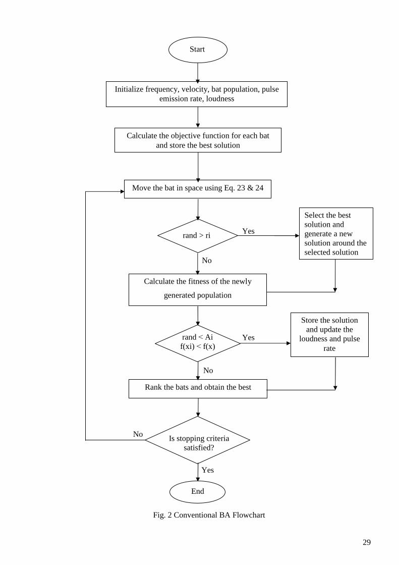
29
Fig. 2 Conventional BA Flowchart
Initialize frequency, velocity, bat population, pulse emission rate, loudness
Calculate the objective function for each bat and store the best solution
Move the bat in space using Eq. 23 & 24
Calculate the fitness of the newly
generated population
Select the best solution and generate a new solution around the selected solution
Store the solution and update the
loudness and pulse rate
Is stopping criteria satisfied?
End
Start
Rank the bats and obtain the best
rand > ri
rand ˂ Ai f(xi) ˂ f(x)
No
Yes
No
Yes
Yes
No

30
2.5 HYBRIDIZATION OF EVOLUTIONARY ALGORITHMS TO SOLVE ORPD
The essence of hybridization is to alleviate the limitations of one algorithm with diversification
aspects of the other. Researchers have observed that a combination of one evolutionary algorithm
with either another evolutionary or a conventional algorithm may result in a potent algorithm
capable of dealing with complex optimization problems [90]. In this section an overview of the
attempts made in recent years to hybridize an evolutionary algorithm with either an evolutionary or
a conventional algorithm in solving an ORPD problem will be presented.
Das and Patvardhan [91] presented a method for solving the ORPD problem based on Evolutionary
Strategy (ES). Some major improvements were added to the traditional ES in order to improve the
convergence and to find a better solution. This improved technique is referred to as Hybrid
Evolutionary Strategy (HES). A conscious effort was made in the design of HES to reduce the
number of load flow executions so that computational requirements were within reasonable limits.
In [92], Yang et al. presented an Improved Evolutionary Programming (IEP) and its hybrid version
combined with the nonlinear IP technique to solve ORPD problems. In an IEP method, the common
practices in regulating reactive power were followed in adjusting the mutation direction of control
variables in order to increase the possibility of keeping the state variables within bounds. The IEP
was also hybridized with the IP method to obtain a fast initial solution, which was then used as a
highly evolved individual in the initial population of the improved EP method.
Esmin et al. [93] proposed a Hybrid PSO with Mutation (HPSOM) for loss minimization. The study
was carried out in two steps. In the first step, using the tangent vector technique, the critical area of
the power system was identified under the point of view of voltage instability. In the second step,
after identifying the critical area, the PSO technique was used to calculate the amount of shunt
reactive power compensation of each bus. The HPSOM algorithm is basically the standard PSO
combined with arithmetic mutation. The notion of mutation in the hybrid model was introduced as
in any other genetic algorithm.
By integrating GA with a nonlinear IPM, a novel hybrid method for the ORPD problem was
proposed in [94]. The method was divided into two parts. The first part was to solve the ORPD with
the IPM by relaxing the discrete variables. The second part was to decompose the original ORPD
into two sub-problems: continuous optimization and discrete optimization. The GA was used to
solve the discrete optimization with the continuous variables being fixed, whereas the IPM solved
the continuous optimization with the discrete variables being constant. The optimal solution was

31
obtained by solving the two sub-problems alternately. A dynamic adjustment strategy was also
presented to make the GA and the IPM to complement each other and to enhance the efficiency of
the hybrid method.
DE is a promising evolutionary algorithm for solving the ORPD problem, but it requires relatively
large population size to avoid premature convergence, which will increase the computational time.
On the other hand, EP has been proved to have a good global search ability. Exploiting this
complementary feature, a hybrid algorithm of DE and EP, denoted as DEEP, was proposed in [95]
to reduce the required population size. The hybridisation was designed as a novel primary–auxiliary
model to minimise the additional computational cost.
In [96], Subbaraj et al. presented a two-phase hybrid PSO approach in solving ORPD problem. In
their hybrid approach, PSO was used to explore the optimal region and a direct search was used as a
local optimization technique for finer convergence.
Fister et al. [97] presented a hybrid tool based on the BA. BA was hybridized with DE strategies.
This hybridization showed very promising results on standard benchmark functions and also
significantly improved the original BA.
Reference [98] presented a reliable and effective algorithm based on Hybrid Modified Imperialist
Competitive Algorithm (MICA) and Invasive Weed Optimization (IWO) for solving the ORPD
problem. The original Imperialist Competitive Algorithm (ICA) often converges to local optima. In
order to avoid this shortcoming, a new method was proposed that profited from the IWO method to
improve local search near the global best and a series of modifications were added to the
assimilation policy rule of ICA in order to further enhance the algorithm's rate of convergence for
achieving a better solution quality.
Mojtaba et al. [99] introduced a hybrid tool to handle the ORPD problem by combining Modified
Teaching Learning Algorithm (MTLA) and Double Differential Evolution (DDE) algorithm. Their
hybrid method also proved to be efficient and showed faster convergence.
In [100], Lenin et al. presented Hybridization of a BA with Harmony Search Algorithm (BAHS) for
solving an ORPD problem. The approach included the addition of a pitch modification procedure in
Harmony Search, serving as a mutation operator during the procedure of the bat updating with the

32
aim of speeding up convergence, thus making the approach more feasible for a wider range of real-
world applications.
Hybridization of a Simulated Annealing and a Nelder-Mead (SANM) algorithm was proposed in
[101] to solve an ORPD problem. The proposed algorithm (SANM) started with a primary solution,
which was generated arbitrarily and then the solution was alienated into partitions. The
neighbourhood zone was generated, an arbitrary number of partitions were selected and a variable
updating procedure was started in order to generate a trail neighbour solution. This process helped
the SANM algorithm to explore the region around the current iterated solution. The Nelder- Mead
(NM) algorithm was used in the final stage in order to progress the best solution found so far and
accelerates the convergence in the final stage.
Singh et al. [102] presented a PSO with an Aging Leader and Challengers (ALC) (denoted as ALC-
PSO) for the solution of an ORPD problem. The ORPD problem was formulated as a nonlinear
constrained single-objective optimization problem where the real power loss and the total voltage
deviation was to be minimized separately.
Reference [103] presented a novel hybrid algorithm combining a Firefly Algorithm (FA) and the
NM simplex method for solving ORPD problems. Like many other general purpose optimization
methods, the original FA often traps into local optima and in order to overcome this shortcoming,
an efficient local search method called the NM simplex subroutine was introduced in the internal
architecture of the original FA algorithm. This method proved to avoid premature convergence of
the original FA by exploration with a FA and exploitation with a NM simplex.
A Hybrid BA (HBA) was proposed in [104] to reduce the real power loss in ORPD problem.
Swarm Intelligence based BA was hybridized with a DE strategy to solve the problem. The HBA
was used to find the optimal settings of generator bus voltage, transformer tap settings and reactive
power of a shunt compensator.
Radosavljevic and Jevtiv [105] presented a new hybrid algorithm (Hybrid GSA-SQP) consisting of
the Gravitational Search Algorithm (GSA) and the Sequential Quadratic Programming (SQP) for
solving the ORPD problem. The performance of this hybrid algorithm for the ORPD problem was
formulated for two different objective functions, namely minimization of real power loss and
voltage profile improvement.

33
Reference [106] presented a hybrid approach based on an ICA and a PSO to find the solution of
ORPD of power systems. This hybrid method was proved to be and has higher capability in finding
better solutions.
2.6 OPTIMAL PLACEMENT OF DG UNIT(S)
Power system generating stations are located either close to the resources (water, coal and gas) or
otherwise located far from the load centres. These generating stations are designed to take
advantage of available economies of scale in a site specific manner and are built as “one-off”
custom projects. Over the years, electric power transmission line losses increase as a result of
increasingly age deterioration and capacity constraints upon the transmission networks. This led to
the introduction of a new technology called distributed generation (DG) unit or system. DG units
refer to the installation of small-scale generating technologies or stations from a few kilowatts up to
50 MW to the existing power networks at the distribution level [107]. These small-scale generating
stations, which include but are not limited to photovoltaic (PV) or solar cells (typically rooftop solar
PV); small wind power system or wind turbines and combined heat power (CHP), are connected in
parallel with the utility power networks. They are located near the consumer loads to reduce
transmission line losses and improve voltage profiles. In general, DG units tend to produce some or
all of the power required by the consumer loads. However, due to the renewable nature of the DG
unit’s energy sources, there are times when these energy sources will be insufficient. In such
circumstances, the consumer will need to receive power from the utility grid. When the DG units
produce more power than the consumer needs at a specific moment, the excess power is available to
the utility grid. The integration of DGs in the distribution network has diverse advantages which
include reduction of active power losses, improvement of voltage profile, reduction of
environmental pollution, less capital intensive, increased efficiency and reliability of the system
network [108].
Numerous methods (conventional and evolutionary techniques) have earlier been used to optimally
install DG unit(s) in the distribution networks to reduce active power transmission line losses. A
number of conventional techniques such as gradient search (GS) [109], linear programming (LP)
[110], Newton-Raphson Extended Method [111] have been successfully applied to optimally install
DG unit(s). While, some evolutionary methods such as GA [112], BA [113], PSO [114, 115], CS
[116], ABC [117], Competitive Swarm Optimizer (CSO) [118], Cat Swarm Optimization (CSO)
[119], Parallel Cat Swarm Optimization Algorithms (PCSO) [119] etc, have also been applied in the
past to optimally install DG unit(s).

34
2.7 SUMMARY
This chapter reviews the development and application of conventional and evolutionary
optimization techniques to solve the ORPD problem by different authors in the field of electrical
power system. It also gives detailed information about ORPD problem formulation and the
application of PSO, as well as BA in solving an ORPD problem. It also reviews the development
and application of some hybrid methods to solve the ORPD as well as optimal placement of DG
unit(s) in the distribution networks to reduce active power transmission line losses. The next chapter
presents the hybridization of PSO and BA to form HPSOBA and show in a flow chat how they can
be used to solve the ORPD problem as well as the simulation results and analysis of using the
proposed hybrid method on the test cases.

35
CHAPTER 3
HYBRID PSO-BA MODEL
This chapter covers the hybridization tool used in this research and the proposed methodology for
the hybridization. There are different methods by which these two optimization techniques can be
hybridized so as to come up with a better method to solve the problem at hand. This chapter
presents the hybridization of PSO and BA to form HPSOBA and the details of the proposed
methodology.
3.1 MOTIVATION FOR HYBRIDIZATION OF PSO WITH BA
The objective function of this research is to minimize the active power loss in a transmission
network using a hybrid algorithm which is a combination of PSO and BA methods. The PSO has
been applied many times to solve optimization problems but in this research considering the PSO’s
shortcomings of premature convergence and required computational time in most cases, an attempt
is made to improve the PSO algorithm. By finding and analyzing a variety of evolutionary
optimization algorithms which were raised in recent years, it was found that the BA is gradually and
excellently applied in the field of power systems. Although the BA cannot guarantee a fast
convergence because it completely depends on random walk, it is proficient at controlling the
exploration and exploitation of the search space and also requires less computational time. Thus
exploring their possible hybridization is a step in the right direction to solve power system
optimization problems.
The use of hybrid algorithms is a new and successful trend in solving optimization problems. The
main aim of this research is to obtain a better performing algorithm that combines the advantages of
individual algorithms. Hybrid algorithms benefit from synergy. However, choosing an adequate
combination of component algorithms to achieve a better overall performance in a particular
situation or problem is important. This research tends to combine the PSO and BA optimization
techniques to form a hybrid tool that can out-perform the algorithms when individually applied in
solving power system optimization problems.
At the start of every optimization process, a global exploration of the search space is required to
probe a wider region for the perspective solution and later on search for a better solution in the
vicinity of a given starting solution within a more promising region. PSO can quickly identify

36
promising areas in the search space while BA can quickly determine the best solution within those
areas.
PSO, which is one of the most popular meta-heuristic approaches, is based on information sharing
among the particles and is transmitted by the most optimistic, global best particle to other particles.
One of the main advantages of PSO, rapid convergence, can also be its main weakness, as
premature convergence to a suboptimal solution may stagnate the swarm without any pressure to
continue exploration. The PSO algorithm has found it difficult to converge to an optimal solution as
the particles arrive in the vicinity of the optimal solution and thus causes slow convergence in the
refined search stage.
On the other hand, the BA has a capability of automatically zooming into a region where promising
solutions have been found and also a strong local search ability controlled by the loudness and pulse
rate. The local search method is applied by using a random walk method in order to refine the best-
found solution at each iteration. Despite its less computational time advantage, it converges very
quickly at the early stage and then convergence rate slows down.
In order to alleviate the drawbacks of both PSO and BA optimization techniques a new hybrid
algorithm, the HPSOBA, is proposed.
3.2 PROPOSED HYBRID PSO-BA (HPSOBA) METHODOLOGY
The proposed HPSOBA optimization method by this research, integrated the respective advantages
of PSO and BA to form a hybrid PSO with a BA denoted as HPSOBA. It combines the fast
convergence ability of a PSO with the less computation time ability of a BA to get a better optimal
solution. The PSO’s Eq. (15) was modified by introducing the BA’s frequency fi as shown in Eq.
(29) below for the HPSOBA. The frequency fi, which controls the pace and range of the movement
of the swarming particles, is generated as shown in Eq. (22). Maximum number of iterations is set
as a stopping criterion.
Vi k+1 = w*V i
k + (c1*rand*(Pbesti k – Xi
k) + c2*rand*(Gbest k – Xi
k)) * f i (29)
The flowchart in Fig. 3 delineates the steps of the HPSOBA algorithm for solving ORPD and its
pseudo code given as follows:
Step1: The bat solutions Xi and their velocities Vi are initialized
For each bat i, define pulse frequency fi at Xi
Initialize emission pulse rates r and the loudness A
The lower and lower boundaries/limits of every control variables are identified.
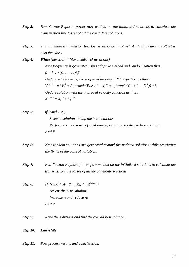
37
Step 2: Run Newton-Raphson power flow method on the initialized solutions to calculate the
transmission line losses of all the candidate solutions.
Step 3: The minimum transmission line loss is assigned as Pbest. At this juncture the Pbest is
also the Gbest.
Step 4: While (iteration < Max number of iterations)
New frequency is generated using adaptive method and randomization thus:
fi = fmin +(fmax - fmin)*β
Update velocity using the proposed improved PSO equation as thus:
Vi k+1 = w*V i
k + (c1*rand*(Pbesti k – Xi
k) + c2*rand*(Gbest k – Xi
k)) * f i
Update solution with the improved velocity equation as thus:
Xi k+1 = Xi
k + Vi k+1
Step 5: if (rand > ri )
Select a solution among the best solutions
Perform a random walk (local search) around the selected best solution
End if
Step 6: New random solutions are generated around the updated solutions while restricting
the limits of the control variables.
Step 7: Run Newton-Raphson power flow method on the initialized solutions to calculate the
transmission line losses of all the candidate solutions.
Step 8: If (rand ˂ Ai & f(Xi) ˂ f(XGbest))
Accept the new solutions
Increase ri and reduce Ai
End if
Step 9: Rank the solutions and find the overall best solution.
Step 10: End while
Step 11: Post process results and visualization.
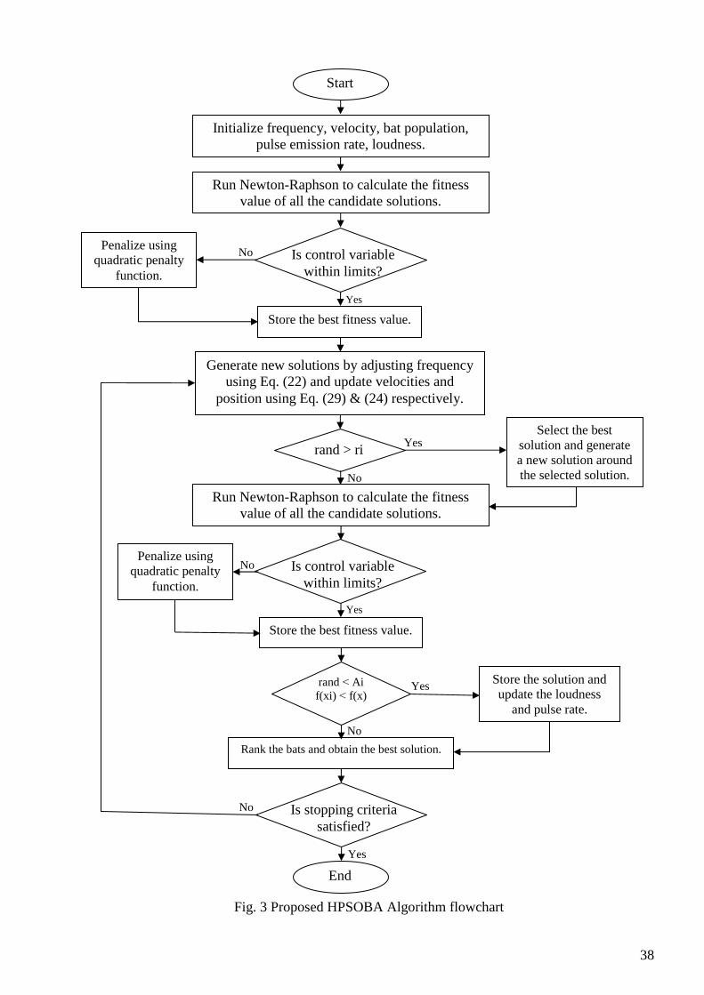
38
Fig. 3 Proposed HPSOBA Algorithm flowchart
Initialize frequency, velocity, bat population, pulse emission rate, loudness.
Run Newton-Raphson to calculate the fitness value of all the candidate solutions.
Store the best fitness value.
Penalize using quadratic penalty
function.
Select the best solution and generate a new solution around the selected solution.
Store the solution and update the loudness
and pulse rate.
Rank the bats and obtain the best solution.
solution
Generate new solutions by adjusting frequency using Eq. (22) and update velocities and
position using Eq. (29) & (24) respectively.
Run Newton-Raphson to calculate the fitness value of all the candidate solutions.
Start
Is control variable within limits?
rand > ri
Store the best fitness value.
Is control variable within limits?
rand ˂ Ai f(xi) ˂ f(x)
Is stopping criteria satisfied?
End
Penalize using quadratic penalty
function.
No
Yes
Yes
No
Yes
No
Yes
No
No
Yes

39
3.3 TEST FUNCTION OPTIMIZATION USING HPSOBA
Test functions also known as standard benchmarks play an important role in validating and
comparing the general performance, convergence rate, accuracy and robustness of optimization
algorithms [120]. The test functions should have some diverse properties, which can be useful in
testing of any new algorithm. The efficiency, reliability and validation of optimization algorithms
can be done by using a set of standard benchmarks or test functions. For any new optimization
technique, it is necessary to validate its performance and compare it with other existing algorithms
using a good set of test functions. These test functions whose details such as search range and
optima positions were provided, were applied to the proposed HPSOBA method to assess its
performance and robustness. PSO and BA methods were also developed in the course of developing
the proposed HPSOBA method.
3.3.1 SIMULATION RESULTS AND ANALYLSIS OF TEST FUNCTION
OPTIMIZATION
The proposed hybrid approach (HPSOBA) including the other two approaches (PSO and BA)
developed by this research were first tested on three standard benchmark/test functions to confirm
their accuracy and robustness. The test functions used for this case study include Griewank,
Rastrigin and Schwefel. The results of this research’s extensive numerical experiments are
summarized in Table I. The table shows the results of PSO, BA and HPSOBA optimization
methods for solving the test functions with dimensions d = 5, 30 and 100. The maximum number of
iterations and number of bats or particles are 2000 and 10 respectively. Each method was performed
for 30 trials to solve the given test function problem.
Griewank Function
(30)
xi ∈ [-600, 600], for all i = 1, …, d
Rastrigin Function
(31)
xi ∈ [-5.12, 5.12], for all i = 1, …, d
Schwefel Function
(32)
xi2
4000 xi
√ i i = 1
d
i = 1
d
f (x) = ∑ − ∏ cos + 1
f (x) = 10d + ∑[ xi2 − 10 cos(2πxi)]
i = 1
d
f (x) = 418.9829d − ∑ xi sin(√| xi |) i = 1
d

40
xi ∈ [-500, 500], for all i = 1, …, d
TABLE I. COMPARISON BETWEEN DIFFERENT ALGORITHMS ON 3 STANDARD
BENCHMARK FUNCTIONS
ALGORITHM DIMENSIONS VALUE PSO BA HPSOBA
GRIEWANK 5 BEST 57.8285 1.1711 5.4514
WORST 328.2437 260.0861 214.7897
MEAN 157.1529 108.0102 66.7185
STD. DEV 68.0770 64.1219 47.5775
30 BEST 522.9148 16.1033 101.3931
WORST 1.1506e+03 1.0745e+03 885.3280
MEAN 861.0965 629.3576 534.6278
STD. DEV 149.3709 281.0386 196.5750
100 BEST 2.4095e+03 1.0826e+03 884.6522
WORST 3.5618e+03 3.3493e+03 3.0002e+03
MEAN 2.9961e+03 2.5574e+03 2.3906e+03
STD. DEV 292.2196 532.6977 572.2150
RASTRIGIN 5 BEST -284.8841 -379.7818 -240.4818
WORST 98.9437 121.6203 99.3437
MEAN 23.1221 10.6579 -0.2336
STD. DEV 92.3501 122.5785 103.1661
30 BEST -162.9674 -789.3809 -1.0689e+03
WORST 569.9399 655.3263 638.5661
MEAN 377.1201 353.9556 336.1339
STD. DEV 158.1019 326.2176 394.9394
100 BEST 1.6055e+03 561.5273 1.1438e+03
WORST 1.9659e+03 2.1029e+03 1.9657e+03
MEAN 1.7608e+03 1.7002e+03 1.6662e+03
STD. DEV 100.1611 292.4334 225.8081
SCHWEFEL 5 BEST -2.5234e+03 -1.2745e+04 -1.8619e+04
WORST 3.1426e+03 2.7637e+03 3.0274e+03
MEAN 1.8502e+03 -2.6896e+03 -2.7273e+03
STD. DEV 1.4914e+03 5.0362e+03 6.6470e+03
30 BEST -2.1333e+04 -6.8378e+04 -4.7411e+04
WORST 1.6043e+04 1.4204e+04 1.4623e+04
MEAN 8.9964e+03 -3.0271e+03 -6.0857e+03
STD. DEV 8.8948e+03 2.2048e+04 1.9236e+04
100 BEST -1.2534e+03 -5.4329e+04 -9.1366e+04
WORST 4.4911e+04 4.3968e+04 4.4159e+04
MEAN 3.4320e+04 2.0747e+04 1.2664e+04

41
STD. DEV 1.0954e+04 2.5903e+04 3.9666e+04
As reflected in Table I, the proposed hybrid algorithm (HPSOBA) when tested on the chosen
standard benchmark/test functions (Griewank, Rastrigin and Schwefel) outperformed the other two
approaches (PSO and BA) also developed and analyzed by this research for 5, 30 and 100 different
dimensions.
3.4 SOLVING ORPD USING HPSOBA
This section presents the simulation results and analysis of using the proposed HPSOBA algorithm
to solve an ORPD problem. There are two case studies conducted as part of this resarch in solving
an ORPD problem. The first case study deals with solving an ORPD problem (active power
transmission line loss minimization objective function) without a DG unit installed using the
proposed HPSOBA approach on IEEE 30- and 118-bus systems, while the second case study is
about installing a new DG unit in the distribution system (load bus) and using the proposed hybrid
approach (HPSOBA) only to optimally place the DG unit on a modified IEEE 30-bus system for
active power transmission line loss minimization.
3.4.1 CASE 1: SIMULATION RESULTS AND ANALYSIS OF SOLVING AN ORPD
WITHOUT A DG UNIT
The proposed HPSOBA optimization method alongside PSO and BA were tested on the IEEE 30-
bus and 118-bus test systems with an objective function of minimizing the active power
transmission losses in an electric power system. The data for these systems can be found in [100].
The algorithms of the PSO, BA and HPSOBA methods were coded in MATLAB R2012b
incorporated with MATPOWER 5.1 and run on an Intel (R) Pentium (R) CPU @ 2.00 GHz with 2
GB of RAM PC. The parameters and data settings of the proposed algorithms for the test systems
are summarized in Table II. Due to the randomness in the PSO, BA and HPSOBA techniques, each
method was executed for 30 runs to solve the given ORPD problem (without a DG unit installed)
objective function when applied to the test systems.
TABLE II. PARAMETERS AND DATA SETTINGS FOR THE PROPOSED ALGORITHMS
PARAMETER SYMBOL PSO BA HPSOBA
Swarm/Bat size N 50 20 20
Maximum number of iterations Iteration/N_gen 200 200 200
Number of variables nvars/d 12 12 12
Acceleration constants c1= c2 2.05 - 2.05
Adaptive inertia weight w 0.9 - 0.4 0.9 - 0.4 0.9 - 0.4

42
PARAMETER SYMBOL PSO BA HPSOBA
Minimum frequency fmin - 0 0
Maximum frequency fmax - 2 2
Minimum pulse rate rmin - 0 0
Maximum pulse rate rmax - 1 1
Minimum loudness Amin - 1 1
Maximum loudness Amax - 2 2
Loudness constant α - 0.99 0.99
Pulse rate constant γ - 0.9 0.9
Constriction factor χ 0.729 - -
3.4.1.1 IEEE 30-BUS TEST SYSTEM
In order to validate the proposed hybrid approach (HPSOBA) for ORPD without a DG unit as well
as the PSO and BA developed in the course of achieving the hybrid approach, an IEEE 30-bus test
system was used. The single-line diagram of the IEEE 30-bus test case is shown in Fig. 4. It
consists of six generator buses, 24 load buses and 41 branches in which four branches are tap
changing transformers branches at lines 6-9, 6-10, 4-12, and 28-27. In addition, buses 10 and 24
have been selected as shunt VAR compensation buses. Hence, a total of 12 optimized control
variables were taken for this ORPD problem. The branch parameters and loads were taken from
[121].
Fig. 4 Single-line diagram of IEEE 30-bus test system [122].

43
The test was carried out by solving the ORPD problem of the active power transmission loss
objective in which variable limits (as given in Table III) were used as system constraints. For
comparison purposes, Newton-Raphson Method, PSO, BA and HPSOBA optimization methods
were applied to solve this test case and compared with other methods in the literature. The initial
system loads, total generation and power losses for IEEE 30-bus system from the actual load flow
study using Newton-Raphson method (base case) are given as follows:
Pload = 283.40; Qload = 126.20
The initial total generation and power losses are as follows:
PG = 301.21; QG = 160.94
Ploss = 17.807; Qloss = 69.61
TABLE III. IEEE 30-BUS TEST SYSTEM CONTROL VARIABLE LIMITS FOR ORPD
CONTROL VARIABLES (p.u) MINIMUM MAXIMUM
Generator Voltage 0.95 1.10
Transformer Tap Setting 0.90 1.10
Reactive Power Compensation 0.00 0.20
The average convergence curves of the PSO, BA and HPSOBA techniques are shown in Figs. 5-7
respectively for IEEE 30-bus test system. Delving into the figures, it will be observed that the
HPSOBA hybrid approach showed better convergence characteristics than the PSO and BA
methods. While the PSO in Fig. 5 starts converging at about the 48th iteration, the BA in Fig. 6
starts to converge at about the 110th iteration and the HPSOBA in Fig. 7 starts to converge at about
the 30th iteration.
Fig. 5 Average convergence curve of the PSO
Convergence Point

44
Fig. 6 Average convergence curve of the BA
Fig. 7 Average convergence curve of the HPSOBA
The simulation results of this research for solving an ORPD (without a DG unit) on an IEEE 30-bus
system were compared with the results of PSO, DE, DE-ABC and ABC algorithms from previous
studies as shown in Table IV. The table shows that the other two algorithms (PSO and BA)
outperformed the results of the previous studies in the literature and the Newton-Raphson method
Convergence Point
Convergence Point

45
(base case), while the proposed hybrid approach (HPSOBA) developed by this research
outperformed all.
TABLE IV. COMPARATIVE RESULTS OF IEEE 30-BUS TEST SYSTEM
ALGORITHM
ACTIVE POWER LOSSES (MW)
Min.
Losses
Max.
Losses
Mean
Losses
Std.
Deviation
BASE CASE - - 17.807 -
PSO [123] - - 16.1810 -
DE [124] 16.2184 16.6272 16.1376 0.089508
DE-ABC [124] 16.2163 16.2164 16.2163 2.34e-05
ABC [124] 16.2325 17.693 16.5908 0.034919
PSO 16.163 16.166 16.165 7.65e-04
BA 16.061 16.185 16.133 2.79e-02
HPSOBA 16.059 16.169 16.125 2.80e-02
Table V shows values of the various control variables after optimization for the PSO, BA, and
HPSOBA algorithms. It can be observed from the table that the control variables are restricted
within their respective constraint’s limits and inviolate. Further more, Table V also showed that the
HPSOBA computation time of 257.01 seconds outperforms that of the PSO and BA. Vg indicates
generated voltage, T indicates transformer tap setting and Qc indicates shunt compensation
respectively in p.u. These optimal setting of various control variables minimizes the objective
function to an optimum solution after a maximum of 200 iterations.
TABLE V. VALUES OF CONTROL VARIABLES BEFORE AND AFTER OPTIMIZATION
FOR IEEE 30-BUS TEST SYSTEM
CONTROL
VARIABLES (p.u)
BASE
CASE
PSO BA HPSOBA
Vg1 1.06 1.10 1.10 1.10
Vg2 1.04 1.09 1.09 1.09
Vg5 1.01 1.05 1.05 1.05
Vg8 1.01 1.06 1.06 1.06
Vg11 1.08 1.10 1.10 1.10
Vg13 1.07 1.10 1.10 1.10
T9-6 0.98 1.06 1.02 1.02
T10-6 0.97 0.90 0.98 0.96
T12-4 0.93 1.05 0.99 1.06
T28-27 0.97 0.98 0.99 0.98

46
CONTROL
VARIABLES (p.u)
BASE
CASE
PSO BA HPSOBA
Qc10 0.19 0.15 0.10 0.11
Qc24 0.04 0.15 01.0 0.10
POWER LOSS (MW) 17.807 16.165 16.133 16.125
CPU TIME (s) - 744.50 273.20 257.01
3.4.1.2 IEEE 118-BUS TEST SYSTEM
To further test the proposed technique in solving an ORPD without a DG unit on a large-scale
power system, a standard IEEE 118-bus test system was considered. The single-line diagram of the
IEEE 118-bus test case is shown in Fig. 8. The test case system has 77 dimensions/variables, that is
54 generator buses, 64 load buses, 186 transmission lines, 9 transformer taps and 14 reactive power
sources. The system line and bus data were taken from [121].
Fig. 8 Single-line diagram of IEEE 118-bus test system [125].
The maximum and minimum limits of reactive power sources, voltage and tap setting limits were
given in Table VI, while the initial values of the control variables are in Table VIII. The initial
system loads, total generation and power losses for an IEEE 118-bus system from the actual load
flow study using Newton-Raphson method are as follows:
Pload = 4242.00; Qload = 1438.00

47
The initial total generation and power losses are as follows:
PG = 4375.35; QG = 881.06
Ploss = 133.350; Qloss = 785.09
TABLE VI. IEEE 118-BUS TEST SYSTEM CONTROL VARIABLE LIMITS FOR ORPD
CONTROL VARIABLES (p.u) MMINMUM MAXIMUM
Generator Voltage 0.95 1.10
Transformer Tap Setting 0.90 1.10
Reactive Power Compensation 0.00 0.25
Figs. 9-11 below show the average convergence curves of PSO, BA and HPSOBA techniques
respectively for an IEEE 118-bus system. Delving into the figures, it will be observed that the
HPSOBA hybrid approach showed better convergence characteristics than the PSO and BA
techniques. While the PSO in Fig. 9 showed a little irregular convergence trait, the BA in Fig. 10
starts to converge at about the 175th iteration and the HPSOBA in Fig. 11 starts to converge at about
the 65th iteration.
Fig. 9 Average convergence curve of the PSO
Convergence Point

48
Fig. 10 Average convergence curve of the BA
Fig. 11 Average convergence curve of the HPSOBA
The simulation results achieved without a DG unit on an IEEE 118-bus system were compared with
the results of the PSO, CLPSO, GSA and OGSA algorithms from previous studies as shown in
Table VII. The table shows that the other two algorithms (PSO and BA) outperformed the results of
the Newton-Raphson method (base case) and that of the previous studies in the literature, while the
main proposed hybrid approach (HPSOBA) developed by this research outperformed all. Further
Convergence Point
Convergence Point
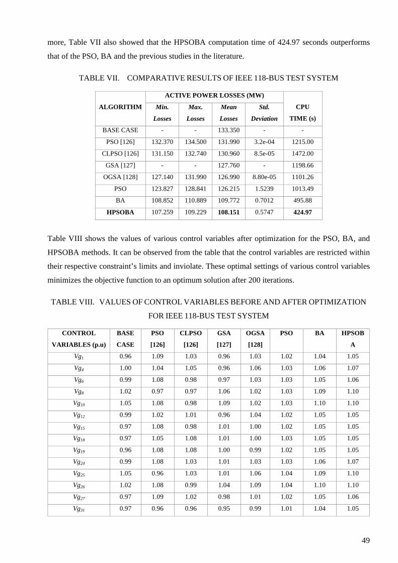
49
more, Table VII also showed that the HPSOBA computation time of 424.97 seconds outperforms
that of the PSO, BA and the previous studies in the literature.
TABLE VII. COMPARATIVE RESULTS OF IEEE 118-BUS TEST SYSTEM
ALGORITHM
ACTIVE POWER LOSSES (MW)
CPU
TIME (s)
Min.
Losses
Max.
Losses
Mean
Losses
Std.
Deviation
BASE CASE - - 133.350 - -
PSO [126] 132.370 134.500 131.990 3.2e-04 1215.00
CLPSO [126] 131.150 132.740 130.960 8.5e-05 1472.00
GSA [127] - - 127.760 - 1198.66
OGSA [128] 127.140 131.990 126.990 8.80e-05 1101.26
PSO 123.827 128.841 126.215 1.5239 1013.49
BA 108.852 110.889 109.772 0.7012 495.88
HPSOBA 107.259 109.229 108.151 0.5747 424.97
Table VIII shows the values of various control variables after optimization for the PSO, BA, and
HPSOBA methods. It can be observed from the table that the control variables are restricted within
their respective constraint’s limits and inviolate. These optimal settings of various control variables
minimizes the objective function to an optimum solution after 200 iterations.
TABLE VIII. VALUES OF CONTROL VARIABLES BEFORE AND AFTER OPTIMIZATION
FOR IEEE 118-BUS TEST SYSTEM
CONTROL
VARIABLES (p.u)
BASE
CASE
PSO
[126]
CLPSO
[126]
GSA
[127]
OGSA
[128]
PSO BA HPSOB
A
Vg1 0.96 1.09 1.03 0.96 1.03 1.02 1.04 1.05
Vg4 1.00 1.04 1.05 0.96 1.06 1.03 1.06 1.07
Vg6 0.99 1.08 0.98 0.97 1.03 1.03 1.05 1.06
Vg8 1.02 0.97 0.97 1.06 1.02 1.03 1.09 1.10
Vg10 1.05 1.08 0.98 1.09 1.02 1.03 1.10 1.10
Vg12 0.99 1.02 1.01 0.96 1.04 1.02 1.05 1.05
Vg15 0.97 1.08 0.98 1.01 1.00 1.02 1.05 1.05
Vg18 0.97 1.05 1.08 1.01 1.00 1.03 1.05 1.05
Vg19 0.96 1.08 1.08 1.00 0.99 1.02 1.05 1.05
Vg24 0.99 1.08 1.03 1.01 1.03 1.03 1.06 1.07
Vg25 1.05 0.96 1.03 1.01 1.06 1.04 1.09 1.10
Vg26 1.02 1.08 0.99 1.04 1.09 1.04 1.10 1.10
Vg27 0.97 1.09 1.02 0.98 1.01 1.02 1.05 1.06
Vg31 0.97 0.96 0.96 0.95 0.99 1.01 1.04 1.05
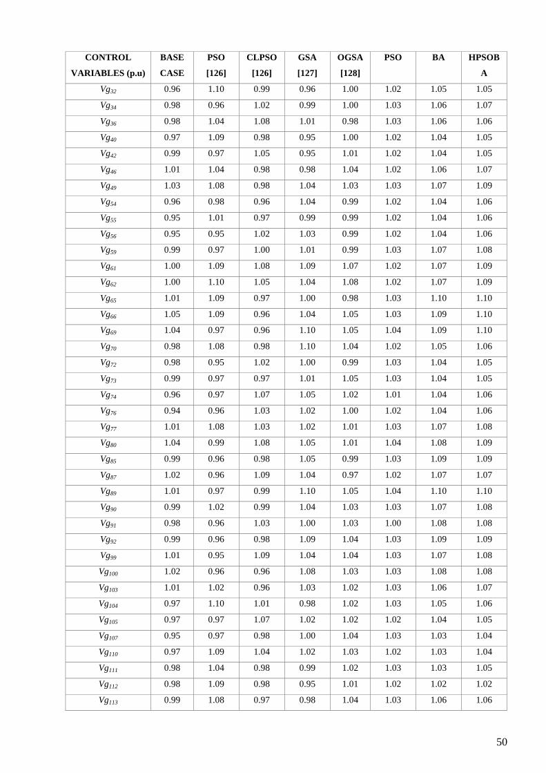
50
CONTROL
VARIABLES (p.u)
BASE
CASE
PSO
[126]
CLPSO
[126]
GSA
[127]
OGSA
[128]
PSO BA HPSOB
A
Vg32 0.96 1.10 0.99 0.96 1.00 1.02 1.05 1.05
Vg34 0.98 0.96 1.02 0.99 1.00 1.03 1.06 1.07
Vg36 0.98 1.04 1.08 1.01 0.98 1.03 1.06 1.06
Vg40 0.97 1.09 0.98 0.95 1.00 1.02 1.04 1.05
Vg42 0.99 0.97 1.05 0.95 1.01 1.02 1.04 1.05
Vg46 1.01 1.04 0.98 0.98 1.04 1.02 1.06 1.07
Vg49 1.03 1.08 0.98 1.04 1.03 1.03 1.07 1.09
Vg54 0.96 0.98 0.96 1.04 0.99 1.02 1.04 1.06
Vg55 0.95 1.01 0.97 0.99 0.99 1.02 1.04 1.06
Vg56 0.95 0.95 1.02 1.03 0.99 1.02 1.04 1.06
Vg59 0.99 0.97 1.00 1.01 0.99 1.03 1.07 1.08
Vg61 1.00 1.09 1.08 1.09 1.07 1.02 1.07 1.09
Vg62 1.00 1.10 1.05 1.04 1.08 1.02 1.07 1.09
Vg65 1.01 1.09 0.97 1.00 0.98 1.03 1.10 1.10
Vg66 1.05 1.09 0.96 1.04 1.05 1.03 1.09 1.10
Vg69 1.04 0.97 0.96 1.10 1.05 1.04 1.09 1.10
Vg70 0.98 1.08 0.98 1.10 1.04 1.02 1.05 1.06
Vg72 0.98 0.95 1.02 1.00 0.99 1.03 1.04 1.05
Vg73 0.99 0.97 0.97 1.01 1.05 1.03 1.04 1.05
Vg74 0.96 0.97 1.07 1.05 1.02 1.01 1.04 1.06
Vg76 0.94 0.96 1.03 1.02 1.00 1.02 1.04 1.06
Vg77 1.01 1.08 1.03 1.02 1.01 1.03 1.07 1.08
Vg80 1.04 0.99 1.08 1.05 1.01 1.04 1.08 1.09
Vg85 0.99 0.96 0.98 1.05 0.99 1.03 1.09 1.09
Vg87 1.02 0.96 1.09 1.04 0.97 1.02 1.07 1.07
Vg89 1.01 0.97 0.99 1.10 1.05 1.04 1.10 1.10
Vg90 0.99 1.02 0.99 1.04 1.03 1.03 1.07 1.08
Vg91 0.98 0.96 1.03 1.00 1.03 1.00 1.08 1.08
Vg92 0.99 0.96 0.98 1.09 1.04 1.03 1.09 1.09
Vg99 1.01 0.95 1.09 1.04 1.04 1.03 1.07 1.08
Vg100 1.02 0.96 0.96 1.08 1.03 1.03 1.08 1.08
Vg103 1.01 1.02 0.96 1.03 1.02 1.03 1.06 1.07
Vg104 0.97 1.10 1.01 0.98 1.02 1.03 1.05 1.06
Vg105 0.97 0.97 1.07 1.02 1.02 1.02 1.04 1.05
Vg107 0.95 0.97 0.98 1.00 1.04 1.03 1.03 1.04
Vg110 0.97 1.09 1.04 1.02 1.03 1.02 1.03 1.04
Vg111 0.98 1.04 0.98 0.99 1.02 1.03 1.03 1.05
Vg112 0.98 1.09 0.98 0.95 1.01 1.02 1.02 1.02
Vg113 0.99 1.08 0.97 0.98 1.04 1.03 1.06 1.06
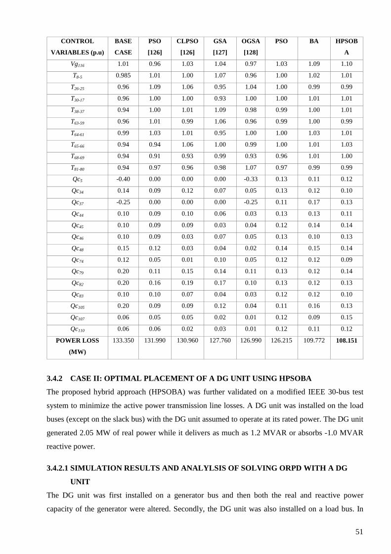
51
CONTROL
VARIABLES (p.u)
BASE
CASE
PSO
[126]
CLPSO
[126]
GSA
[127]
OGSA
[128]
PSO BA HPSOB
A
Vg116 1.01 0.96 1.03 1.04 0.97 1.03 1.09 1.10
T8-5 0.985 1.01 1.00 1.07 0.96 1.00 1.02 1.01
T26-25 0.96 1.09 1.06 0.95 1.04 1.00 0.99 0.99
T30-17 0.96 1.00 1.00 0.93 1.00 1.00 1.01 1.01
T38-37 0.94 1.00 1.01 1.09 0.98 0.99 1.00 1.01
T63-59 0.96 1.01 0.99 1.06 0.96 0.99 1.00 0.99
T64-61 0.99 1.03 1.01 0.95 1.00 1.00 1.03 1.01
T65-66 0.94 0.94 1.06 1.00 0.99 1.00 1.01 1.03
T68-69 0.94 0.91 0.93 0.99 0.93 0.96 1.01 1.00
T81-80 0.94 0.97 0.96 0.98 1.07 0.97 0.99 0.99
Qc5 -0.40 0.00 0.00 0.00 -0.33 0.13 0.11 0.12
Qc34 0.14 0.09 0.12 0.07 0.05 0.13 0.12 0.10
Qc37 -0.25 0.00 0.00 0.00 -0.25 0.11 0.17 0.13
Qc44 0.10 0.09 0.10 0.06 0.03 0.13 0.13 0.11
Qc45 0.10 0.09 0.09 0.03 0.04 0.12 0.14 0.14
Qc46 0.10 0.09 0.03 0.07 0.05 0.13 0.10 0.13
Qc48 0.15 0.12 0.03 0.04 0.02 0.14 0.15 0.14
Qc74 0.12 0.05 0.01 0.10 0.05 0.12 0.12 0.09
Qc79 0.20 0.11 0.15 0.14 0.11 0.13 0.12 0.14
Qc82 0.20 0.16 0.19 0.17 0.10 0.13 0.12 0.13
Qc83 0.10 0.10 0.07 0.04 0.03 0.12 0.12 0.10
Qc105 0.20 0.09 0.09 0.12 0.04 0.11 0.16 0.13
Qc107 0.06 0.05 0.05 0.02 0.01 0.12 0.09 0.15
Qc110 0.06 0.06 0.02 0.03 0.01 0.12 0.11 0.12
POWER LOSS
(MW)
133.350 131.990 130.960 127.760 126.990 126.215 109.772 108.151
3.4.2 CASE II: OPTIMAL PLACEMENT OF A DG UNIT USING HPSOBA
The proposed hybrid approach (HPSOBA) was further validated on a modified IEEE 30-bus test
system to minimize the active power transmission line losses. A DG unit was installed on the load
buses (except on the slack bus) with the DG unit assumed to operate at its rated power. The DG unit
generated 2.05 MW of real power while it delivers as much as 1.2 MVAR or absorbs -1.0 MVAR
reactive power.
3.4.2.1 SIMULATION RESULTS AND ANALYLSIS OF SOLVING ORPD WITH A DG
UNIT
The DG unit was first installed on a generator bus and then both the real and reactive power
capacity of the generator were altered. Secondly, the DG unit was also installed on a load bus. In

52
addition to modifying the real and reactive power capacity, the voltage magnitude of the newly
installed DG unit was treated as a new control variable, thereby increasing the total number of
control variables from 12 to 13. Each of the modified DG units installed on the buses were
evaluated for 30 independent runs and the mean value was taken for the real power minimization
objective function. The simulation results were compared with that of a HPSOBA method without a
DG unit installed. The load bus, generator bus and branch parameters of the test system were taken
from [121] while the control variables as well as the installed DG unit’s real and reactive power
limits used as system constraints are as given in Table IX.
TABLE IX. MODIFIED IEEE 30-BUS TEST SYSTEM CONSTRAINTS FOR DG UNIT OPTIMAL INSTALLATION
CONTROL VARIABLES MMINMUM MAXIMUM Generator Voltage (p.u) 0.95 1.10
Transformer Tap Setting (p.u) 0.90 1.10
Reactive Power Compensation (p.u) 0.00 0.20
DG Reactive Power Output (MVAR) -1.0 1.2
DG Real Power Output (MW) 0 2.05
The simulation results of the DG unit’s placements on each load bus except on the slack bus are
shown in Table X and the simulation graph shown in Fig. 12. It is observed that installing the DG
unit on bus 24 gave the best result of 15.738MW as indicated in bold in the table. That is an 11.62%
real power transmission line loss reduction, making bus 24 the optimum location. It can also be
observed from Table X that installing the DG unit on bus 18 gave the best computation time of
230.92 seconds (also indicated in bold in the table).
TABLE X. COMPARATIVE RESULTS OF THE DG UNIT PLACEMENT ON EACH BUS
Bus No Loss (MW)
Loss Reduction (%)
CPU Time (s)
1 0 0 -
2 16.026 10.00 243.35
3 15.988 10.22 240.65
4 15.924 10.57 245.12
5 15.861 10.93 272.11
6 15.829 11.11 250.94
7 15.835 11.07 247.25
8 15.883 10.80 238.33
9 15.820 11.16 241.20
10 15.819 11.16 252.44
11 15.910 10.65 261.23
12 15.901 10.70 239.78
13 15.947 10.45 254.09
14 15.891 10.76 243.95

53
Bus No Loss (MW)
Loss Reduction (%)
CPU Time (s)
15 15.856 10.96 240.28
16 15.894 10.74 232.29
17 15.850 10.99 238.93
18 15.820 11.16 230.92
19 15.815 11.19 266.78
20 15.838 11.06 255.63
21 15.759 11.50 231.99
22 15.789 11.33 298.63
23 15.790 11.33 237.45
24 15.738 11.62 238.26
25 15.831 11.10 237.34
26 15.807 11.23 237.07
27 15.881 10.82 246.02
28 15.882 10.81 245.91
29 15.870 10.88 236.88
30 15.793 11.31 232.02
Fig. 12 Graph of the comparative results of the DG unit placement on each bus
Table XI showed the comparative results of the proposed HPSOBA approach with and without the
DG unit placement on each load bus. The table showed that the proposed HPSOBA algorithm
developed by this research have better results when the DG unit is installed on bus 24 than without
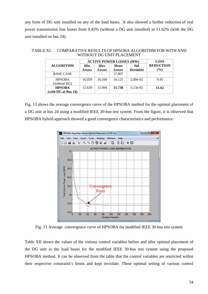
54
any form of DG unit installed on any of the load buses. It also showed a further reduction of real
power transmission line losses from 9.45% (without a DG unit installed) to 11.62% (with the DG
unit installed on bus 24).
TABLE XI. COMPARATIVE RESULTS OF HPSOBA ALGORITHM FOR WITH AND WITHOUT DG UNIT PLACEMENT
ALGORITHM ACTIVE POWER LOSSES (MW) LOSS
REDUCTION (%)
Min. Losses
Max. Losses
Mean Losses
Std. Deviation
BASE CASE - - 17.807 - -
HPSOBA (without DG)
16.059 16.169 16.125 2.80e-02 9.45
HPSOBA (with DG at Bus 24)
15.639 15.894 15.738 5.13e-02 11.62
Fig. 13 shows the average convergence curve of the HPSOBA method for the optimal placement of
a DG unit at bus 24 using a modified IEEE 30-bus test system. From the figure, it is observed that
HPSOBA hybrid approach showed a good convergence characteristics and performance.
Fig. 13 Average convergence curve of HPSOBA for modified IEEE 30-bus test system
Table XII shows the values of the various control variables before and after optimal placement of
the DG unit in the load buses for the modified IEEE 30-bus test system using the proposed
HPSOBA method. It can be observed from the table that the control variables are restricted within
their respective constraint’s limits and kept inviolate. These optimal setting of various control
Convergence Point
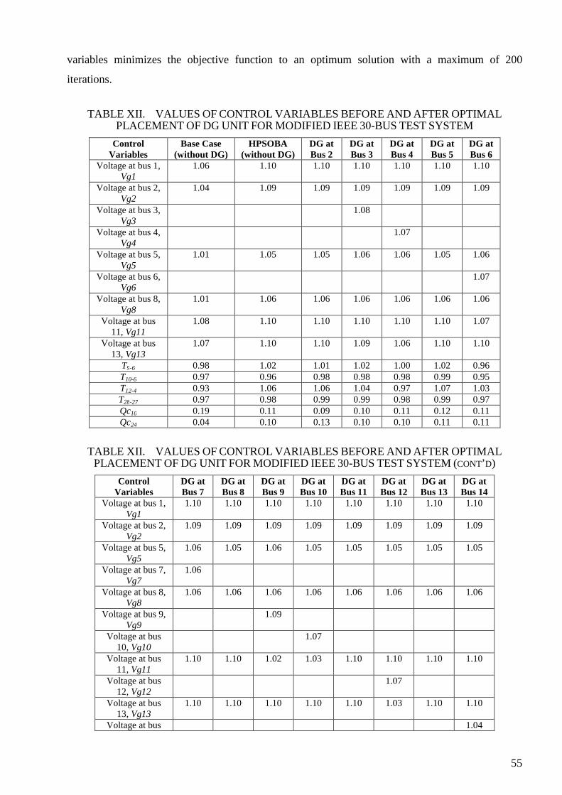
55
variables minimizes the objective function to an optimum solution with a maximum of 200
iterations.
TABLE XII. VALUES OF CONTROL VARIABLES BEFORE AND AFTER OPTIMAL PLACEMENT OF DG UNIT FOR MODIFIED IEEE 30-BUS TEST SYSTEM
Control Variables
Base Case (without DG)
HPSOBA (without DG)
DG at Bus 2
DG at Bus 3
DG at Bus 4
DG at Bus 5
DG at Bus 6
Voltage at bus 1, Vg1
1.06 1.10 1.10 1.10 1.10 1.10 1.10
Voltage at bus 2, Vg2
1.04 1.09 1.09 1.09 1.09 1.09 1.09
Voltage at bus 3, Vg3
1.08
Voltage at bus 4, Vg4
1.07
Voltage at bus 5, Vg5
1.01 1.05 1.05 1.06 1.06 1.05 1.06
Voltage at bus 6, Vg6
1.07
Voltage at bus 8, Vg8
1.01 1.06 1.06 1.06 1.06 1.06 1.06
Voltage at bus 11, Vg11
1.08 1.10 1.10 1.10 1.10 1.10 1.07
Voltage at bus 13, Vg13
1.07 1.10 1.10 1.09 1.06 1.10 1.10
T9-6 0.98 1.02 1.01 1.02 1.00 1.02 0.96 T10-6 0.97 0.96 0.98 0.98 0.98 0.99 0.95 T12-4 0.93 1.06 1.06 1.04 0.97 1.07 1.03 T28-27 0.97 0.98 0.99 0.99 0.98 0.99 0.97 Qc10 0.19 0.11 0.09 0.10 0.11 0.12 0.11 Qc24 0.04 0.10 0.13 0.10 0.10 0.11 0.11
TABLE XII. VALUES OF CONTROL VARIABLES BEFORE AND AFTER OPTIMAL PLACEMENT OF DG UNIT FOR MODIFIED IEEE 30-BUS TEST SYSTEM (CONT’D)
Control Variables
DG at Bus 7
DG at Bus 8
DG at Bus 9
DG at Bus 10
DG at Bus 11
DG at Bus 12
DG at Bus 13
DG at Bus 14
Voltage at bus 1, Vg1
1.10 1.10 1.10 1.10 1.10 1.10 1.10 1.10
Voltage at bus 2, Vg2
1.09 1.09 1.09 1.09 1.09 1.09 1.09 1.09
Voltage at bus 5, Vg5
1.06 1.05 1.06 1.05 1.05 1.05 1.05 1.05
Voltage at bus 7, Vg7
1.06
Voltage at bus 8, Vg8
1.06 1.06 1.06 1.06 1.06 1.06 1.06 1.06
Voltage at bus 9, Vg9
1.09
Voltage at bus 10, Vg10
1.07
Voltage at bus 11, Vg11
1.10 1.10 1.02 1.03 1.10 1.10 1.10 1.10
Voltage at bus 12, Vg12
1.07
Voltage at bus 13, Vg13
1.10 1.10 1.10 1.10 1.10 1.03 1.10 1.10
Voltage at bus 1.04

56
14, Vg14 T9-6 1.01 1.02 1.03 1.05 1.01 0.99 1.01 1.01 T10-6 0.98 0.97 1.00 1.02 0.98 0.96 0.99 0.99 T12-4 1.05 1.06 1.02 1.01 1.06 1.07 1.06 1.06 T28-27 0.98 0.98 0.97 0.96 0.98 0.97 0.98 0.99 Qc10 0.10 0.08 0.09 0.10 0.09 0.08 0.10 0.10 Qc24 0.10 0.11 0.09 0.10 0.10 0.11 0.12 0.09
TABLE XII. VALUES OF CONTROL VARIABLES BEFORE AND AFTER OPTIMAL PLACEMENT OF DG UNIT FOR MODIFIED IEEE 30-BUS TEST SYSTEM (CONT’D)
Control Variables
DG at Bus 15
DG at Bus 16
DG at Bus 17
DG at Bus 18
DG at Bus 19
DG at Bus 20
DG at Bus 21
DG at Bus 22
Voltage at bus 1, Vg1
1.10 1.10 1.10 1.10 1.10 1.10 1.10 1.10
Voltage at bus 2, Vg2
1.09 1.09 1.09 1.09 1.09 1.09 1.09 1.09
Voltage at bus 5, Vg5
1.06 1.06 1.05 1.05 1.06 1.05 1.05 1.05
Voltage at bus 8, Vg8
1.06 1.06 1.06 1.06 1.06 1.06 1.06 1.06
Voltage at bus 11, Vg11
1.10 1.10 1.10 1.10 1.10 1.10 1.10 1.10
Voltage at bus 13, Vg13
1.10 1.10 1.10 1.10 1.10 1.10 1.10 1.10
Voltage at bus 15, Vg15
1.05
Voltage at bus 16, Vg16
1.04
Voltage at bus 17, Vg17
1.06
Voltage at bus 18, Vg18
1.04
Voltage at bus 19, Vg19
1.03
Voltage at bus 20, Vg20
1.04
Voltage at bus 21, Vg21
1.05
Voltage at bus 22, Vg22
1.05
T9-6 1.00 1.02 1.01 1.01 1.03 1.02 1.02 1.03 T10-6 1.00 0.99 0.98 0.99 0.99 0.99 1.00 0.99 T12-4 1.06 1.06 1.04 1.05 1.06 1.05 1.03 1.04 T28-27 0.99 0.99 0.97 0.98 0.98 0.99 0.97 0.98 Qc10 0.10 0.09 0.10 0.15 0.11 0.10 0.10 0.11 Qc24 0.13 0.09 0.11 0.09 0.11 0.09 0.08 0.09
TABLE XII. VALUES OF CONTROL VARIABLES BEFORE AND AFTER OPTIMAL PLACEMENT OF DG UNIT FOR MODIFIED IEEE 30-BUS TEST SYSTEM (CONT’D)
Control Variables
DG at Bus 23
DG at Bus 24
DG at Bus 25
DG at Bus 26
DG at Bus 27
DG at Bus 28
DG at Bus 29
DG at Bus 30
Voltage at bus 1, Vg1
1.10 1.10 1.10 1.10 1.10 1.10 1.10 1.10
Voltage at bus 2, Vg2
1.09 1.09 1.09 1.09 1.09 1.09 1.09 1.09
Voltage at bus 5, Vg5
1.05 1.05 1.05 1.05 1.05 1.05 1.05 1.05

57
Voltage at bus 8, Vg8
1.06 1.06 1.06 1.06 1.06 1.06 1.06 1.06
Voltage at bus 11, Vg11
1.10 1.10 1.10 1.10 1.10 1.10 1.10 1.10
Voltage at bus 13, Vg13
1.10 1.10 1.10 1.10 1.10 1.10 1.10 1.10
Voltage at bus 23, Vg23
1.04
Voltage at bus 24, Vg24
1.03
Voltage at bus 25, Vg25
1.04
Voltage at bus 26, Vg26
1.03
Voltage at bus 27, Vg27
1.05
Voltage at bus 28, Vg28
1.06
Voltage at bus 29, Vg29
1.03
Voltage at bus 30, Vg30
1.02
T9-6 1.02 1.02 1.01 1.02 1.00 0.99 1.00 1.02 T10-6 0.98 1.01 0.98 0.97 0.98 0.99 1.00 0.97 T12-4 1.06 1.06 1.05 1.06 1.05 1.05 1.06 1.07 T28-27 0.99 1.00 1.00 0.99 1.04 0.98 1.00 1.01 Qc10 0.09 0.10 0.11 0.11 0.10 0.12 0.12 0.12 Qc24 0.10 0.10 0.10 0.13 0.11 0.10 0.12 0.11
3.5 SUMMARY
This chapter dealt with the hybridization of the already chosen optimization techniques and their
step implementation. It also discussed the simulation procedures and results obtained using the
proposed HPSOBA to solve for test function optimization and ORPD problems. The results
obtained from solving the ORPD problem using the HPSOBA considered two case studies of with
and with a DG unit installed. The first case study of solving an ORPD problem without a DG unit
installed was tested of both IEEE 30-bus and 118-bus test systems, while the second case study of
solving an ORPD problem with a DG unit installed was tested on a modified IEEE 30-bus test
system. The simulation results were compared with other evolutionary algorithms in the literature.
The next chapter presents the modification of the proposed HPSOBA to check if there will be
further improvement on its performance or not.

58
CHAPTER 4
MODIFIED HPSOBA
4.1 OVERVIEW
This chapter presents three new modifications embedded into this research’s proposed HPSOBA to
check if there will be further improvement on its performance or not. The modified HPSOBA
denoted as MHPSOBA also followed the line of the HPSOBA in fulfilling the local search by using
the random walk operation mechanism of a BA whereas the global search is accomplished by a
PSO operator. Using this combination it maintains a balance between ‘exploration’ and
‘exploitation’ and enjoying the best of both the algorithms (BA and PSO). The MHPSOBA has the
same pseudo code and flowchart as the proposed HPOSBA. It was also tested on a modified IEEE
30-bus system to solve an ORPD problem (active power transmission line loss minimization
objective function) without a DG unit installed.
4.2 MODIFICATIONS OF HPSOBA
The MHPSOBA method emanated from three new modifications embedded into the proposed
HPSOBA method and is captured in this subsection:
4.2.1 1st MODIFICATION (Pulse Frequency)
Microbats use echolocation as their main navigation system. During their flights, bats emit
continuously short pulses that last a few milliseconds. By analyzing the echoes, they can create a
3D mental image of their surroundings. The information of other bats such as their positions can be
useful to guide the search process. In addition, pulses can travel in different directions and thus it
may be useful to assume that each bat emits two pulses into two different directions before deciding
in which direction it will fly and this feature can be used to simulate the time difference or delay
between echoes received by two ears. It is also assumed that the two pulses emitted have the same
pulse rates but different pulse frequencies f1 and f2. To extend further along this line of thinking, it
can also be assumed that all the bats emit a pulse in the direction of the best bat (solution) where the
food is considered to exist, and the other pulse to the direction of a randomly chosen bat. From the
echoes (feedback), the bat can know if food exists around these two bats or not.
The frequencies f1 and f2 of the two pulses are updated as follows:
fi1= fmin +(fmax - fmin)*rand1 (33)
fi 2= fmin +(fmax - fmin)*rand2 (34)
Both rand1 and rand2 are two random vectors between 0 and 1.
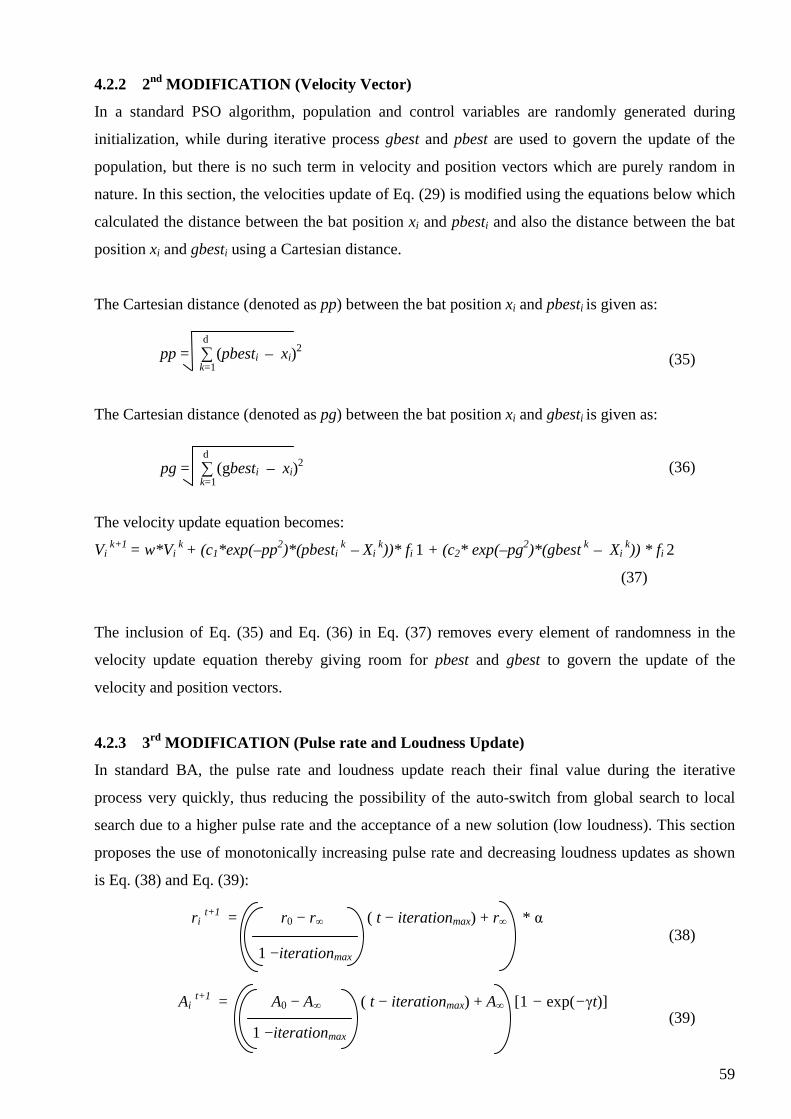
59
4.2.2 2nd MODIFICATION (Velocity Vector)
In a standard PSO algorithm, population and control variables are randomly generated during
initialization, while during iterative process gbest and pbest are used to govern the update of the
population, but there is no such term in velocity and position vectors which are purely random in
nature. In this section, the velocities update of Eq. (29) is modified using the equations below which
calculated the distance between the bat position xi and pbesti and also the distance between the bat
position xi and gbesti using a Cartesian distance.
The Cartesian distance (denoted as pp) between the bat position xi and pbesti is given as:
(35)
The Cartesian distance (denoted as pg) between the bat position xi and gbesti is given as:
(36)
The velocity update equation becomes:
Vi k+1 = w*V i
k + (c1*exp(–pp2)*(pbesti k – Xi
k))* f i 1 + (c2* exp(–pg2)*(gbest k – Xi
k)) * f i 2
(37)
The inclusion of Eq. (35) and Eq. (36) in Eq. (37) removes every element of randomness in the
velocity update equation thereby giving room for pbest and gbest to govern the update of the
velocity and position vectors.
4.2.3 3rd MODIFICATION (Pulse rate and Loudness Update)
In standard BA, the pulse rate and loudness update reach their final value during the iterative
process very quickly, thus reducing the possibility of the auto-switch from global search to local
search due to a higher pulse rate and the acceptance of a new solution (low loudness). This section
proposes the use of monotonically increasing pulse rate and decreasing loudness updates as shown
is Eq. (38) and Eq. (39):
(38)
(39)
pp = ∑ (pbesti – xi)
2 d
k=1
pg = ∑ (gbesti – xi)
2 d
k=1
r i t+1 = r0 − r∞ ( t − iterationmax) + r∞ * α
1 −iterationmax
Ai t+1 = A0 − A∞ ( t − iterationmax) + A∞ [1 − exp(−γt)]
1 −iterationmax
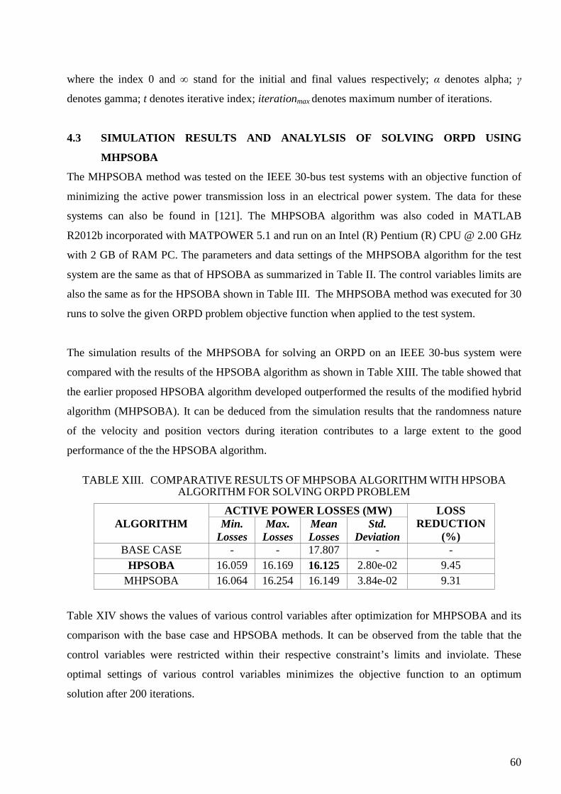
60
where the index 0 and ∞ stand for the initial and final values respectively; α denotes alpha; γ
denotes gamma; t denotes iterative index; iterationmax denotes maximum number of iterations.
4.3 SIMULATION RESULTS AND ANALYLSIS OF SOLVING ORPD USING
MHPSOBA
The MHPSOBA method was tested on the IEEE 30-bus test systems with an objective function of
minimizing the active power transmission loss in an electrical power system. The data for these
systems can also be found in [121]. The MHPSOBA algorithm was also coded in MATLAB
R2012b incorporated with MATPOWER 5.1 and run on an Intel (R) Pentium (R) CPU @ 2.00 GHz
with 2 GB of RAM PC. The parameters and data settings of the MHPSOBA algorithm for the test
system are the same as that of HPSOBA as summarized in Table II. The control variables limits are
also the same as for the HPSOBA shown in Table III. The MHPSOBA method was executed for 30
runs to solve the given ORPD problem objective function when applied to the test system.
The simulation results of the MHPSOBA for solving an ORPD on an IEEE 30-bus system were
compared with the results of the HPSOBA algorithm as shown in Table XIII. The table showed that
the earlier proposed HPSOBA algorithm developed outperformed the results of the modified hybrid
algorithm (MHPSOBA). It can be deduced from the simulation results that the randomness nature
of the velocity and position vectors during iteration contributes to a large extent to the good
performance of the the HPSOBA algorithm.
TABLE XIII. COMPARATIVE RESULTS OF MHPSOBA ALGORITHM WITH HPSOBA ALGORITHM FOR SOLVING ORPD PROBLEM
ALGORITHM ACTIVE POWER LOSSES (MW) LOSS
REDUCTION (%)
Min. Losses
Max. Losses
Mean Losses
Std. Deviation
BASE CASE - - 17.807 - - HPSOBA 16.059 16.169 16.125 2.80e-02 9.45
MHPSOBA 16.064 16.254 16.149 3.84e-02 9.31
Table XIV shows the values of various control variables after optimization for MHPSOBA and its
comparison with the base case and HPSOBA methods. It can be observed from the table that the
control variables were restricted within their respective constraint’s limits and inviolate. These
optimal settings of various control variables minimizes the objective function to an optimum
solution after 200 iterations.

61
TABLE XIV. COMPARATIVE VALUES OF CONTROL VARIABLES AFTER
OPTIMIZATION FOR HPSOBA AND MHPSOBA METHODS FOR IEEE 30-BUS TEST
SYSTEM
CONTROL
VARIABLES (p.u)
BASE
CASE
HPSOBA MHPSOBA
Vg1 1.06 1.10 1.10
Vg2 1.04 1.09 1.09
Vg5 1.01 1.05 1.05
Vg8 1.01 1.06 1.06
Vg11 1.08 1.10 1.10
Vg13 1.07 1.10 1.09
T9-6 0.98 1.02 1.01
T10-6 0.97 0.96 0.99
T12-4 0.93 1.06 1.05
T28-27 0.97 0.98 0.98
Qc10 0.19 0.11 0.12
Qc24 0.04 0.10 0.11
POWER LOSS (MW) 17.807 16.125 16.149
CPU TIME (s) - 257.01 276.24
4.4 SUMMARY
This chapter dealt with the modification of the proposed algorithm denoted as MHPSOBA to check
if there will be further improvement on the performance of the HPSOBA or not. The MHPSOBA
has the same pseudo code and flowchart as the proposed HPOSBA and it was tested on a modified
IEEE 30-bus test system to solve an ORPD problem (active power transmission line loss
minimization objective function) without a DG unit installed. It also discussed the simulation
results obtained from solving the ORPD problem without a DG unit installed using the MHPSOBA.
The simulation results were compared with that of HPSOBA. The next chapter presents the
modification of the proposed HPSOBA to check if there will be further improvement on its
performance or notconclusion and future work.
62
CHAPTER 5
CONCLUSION AND FUTURE WORK
5.1 CONCLUSION
The HPSOBA approach was evaluated and tested on IEEE 30-bus and IEEE 118-bus test systems to
solve the ORPD (with and without DG unit optimally installed) as well as benchmark test functions.
Simulation results confirm the robustness of the proposed HPSOBA algorithm when tested on test
functions such as Griewank, Rastrigin and Schwefel. When tested on the IEEE 30-bus and IEEE
118-bus test systems to solve for the ORPD without a DG unit and on modified IEEE 30-bus test
system for solving an ORPD with a DG unit optimally installed, it was observed that the proposed
HPSOBA algorithm yields optimal settings of the control variables of the test power systems and
reduced the active power transmission line losses with less computational time. The results obtained
from the simulations demonstrate its effectiveness and superiority over the Newton-Raphson
method and other evolutionary algorithms such as PSO, DE, ABC, CLPSO, GSA and OGSA
mentioned in this research in solving the ORPD problem of power systems.
In conclusion, the contributions of this research can be divided into three parts designated as Part I:
benchmark function optimization; Part II: solving the ORPD problem for active power transmission
line loss minimization; and Part III: Modification of the proposed hybrid approach and its test on an
IEEE 30-bus system for solving the ORPD problem.
Contributions of Part I: In solving benchmark functions, the results show that HPSOBA
outperformed the other two algorithms of PSO and BA for both high and low dimensions in terms
of general performance. The proposed method was found to be accurate, robust and efficient.
Contributions of Part II: This can be divided into two case studies namely solving the ORPD
without a DG unit installed and solving the ORPD by optimal installation of a DG unit. For solving
the ORPD problem without a DG unit (first case study), the proposed HPSOBA method was
validated using IEEE 30- and 118- bus test systems. The simulation results show that HPSOBA
method reduced the the active power transmission line losses from 17.807 MW (base case) to
16.125 MW (9.45% loss reduction) for the IEEE 30-bus system and from 133.350 MW (base case)
to 108.151 MW (18.90% loss reduction) for the IEEE 118-bus system.
For the second case study, optimal placement of a DG unit for real power transmission line loss
minimization was successfully solved in this research using the hybrid algorithm (HPSOBA). The

63
proposed algorithm was validated using a modified IEEE 30-bus test system and compared for with
and without a DG unit installed on the load buses. The outcome of the simulation tests proved that
the hybrid approach (HPSOBA) further reduced the real power transmission line losses from 16.125
MW (without DG unit installed) to 15.738 MW (with DG unit installed on bus 24), representing
11.62% loss reduction while maintaining the control variables within their respective limits.
Contributions of Part III: The proposed HPSOBA was modified to check if there will be further
improvement in its performance. The simulation results of the MHPSOBA showed that the earlier
proposed HPSOBA algorithm developed by this research also outperformed the results of this
modified hybrid approach (MHPSOBA). The simulation results also show that the random nature of
the velocity and position vectors during iteration contributes to a large extent to the good
performance of the HPSOBA algorithm.
Summarily, Table XV shows that the hybrid approach (HPSOBA) outperformed the PSO, BA and
MHPSOBA methods for both IEEE 30- and 118- bus test systems.
TABLE XV. ALGORITHM PERFORMANCE SUMMARY FOR SOLVING ORPD PROBLEM
ALGORITHM IEEE 30-BUS
POWER LOSS (MW)
IEEE 118-BUS
POWER LOSS (MW)
BASE CASE 17.807 133.350
PSO 16.165 126.215
BA 16.133 109.772
HPSOBA 16.125 108.151
HPSOBA (with DG at Bus 24)
15.738 -
MHPSOBA 16.149 -
In general, the contributions of this research, apart from optimally installing a DG unit using a
HPSOBA, can be summarized as follows: (1) minimization of active power transmission losses, (2)
load bus voltage levels are maintained within their respective limits, (3) reactive power generation
is kept within limits and (4) transformer tap settings are maintained within limits.
The simulation test results show that the proposed HPSOBA method not only improves the
solution’s quality but also reduces the computational time and is suitable for solving an ORPD,
optimal placement of a DG unit for real power loss minimization as well as benchmark function
optimization problems.

64
5.2 FUTURE WORK
Three areas are proposed for further research:
1) This research considered only one DG unit, further research needs to be done on adding
more DG units in solving an ORPD problem. The computational time must also be
considered.
2) Reduction in computational time of the proposed HPSOBA should be investigated.
3) Application of the proposed HPSOBA on real-world ORPD problems should also be
investigated.

65
LIST OF PUBLICATIONS
1. Agbugba, E., & Wang, Z., “A Hybrid Particle Swarm Optimization with Bat Algorithm
for Optimal Reactive Power Dispatch,” submitted to IEEE Transaction on Power
System with manuscript No: TPWRS-00546-2017, (submitted April 2017).
2. Agbugba, E., & Wang, Z., “Modified Hybrid Particle Swarm Optimization with Bat
Algorithm for Optimal Placement of Distributed Generation,” A draft paper to be
submitted to a conference.

66
REFERENCES
[1] Soliman, S.A., & Mantawy, A.H. (2012). Modern Optimization Techniques with
Applications in Electric Power Systems. Florida, Springer Science LLC. 1–430.
[2] Abhyankar, A. R., & Khaparde, S. A. (2013). Introduction to deregulation in power
industry. Report by Indian Institute of Technology, Mumbai.
[3] Tong, X., Zhang, Y. & Wu, F. (2006) A Decoupled Semi Smooth Newton Method for
Optimal Power Flow. in: IEEE Power Engineering Society General Meeting.
[4] Carpentier, J. (1962) Contribution to the Economic Dispatch Problem. Bullentin de la
Societe Francoise des Electricien. 3 (8), 431–47.
[5] Dommel, H. W. & Tinney, W. F. (1968) Optimal Power Flow Solutions. IEEE
Transactions on Power Apparatus Systems. PAS-87 (10), 1866 –1876.
[6] Zhang, X. P. (2010) Fundamentals of Electric Power Systems. New York, John Wiley &
Sons, Inc. 1–52.
[7] Mamandur, K. R. C. & Chenoweth, R. D. (1981) Optimal Control of Reactive Power flow
for Improvements in Voltage Profiles and for Real Power Loss Minimization. in IEEE
Transactions on Power Apparatus and Systems. PAS-100 (7), 3185–3194.
[8] Biskas, P., Ziogos, N., Tellidou, A., Zoumas, C., Bakirtzis, A., Petridis, V. & Tsakoumis
A. (2005) Comparison of two Metaheuristics with Mathematical Programming Methods
for the Solution of OPF. in: Proceedings of the 13th International Conference on
Intelligent Systems Application to Power Systems.
[9] Bjelogrlic, M.R., Calovic, M.S., Babic, B.S. & Ristanovic, P. (1990) Application of
Newton’s Optimal Power Flow in Voltage/Reactive Power Control. IEEE Trans. on Power
Systems. 5, 1447–1454.
[10] Quintana, V.H. & Nieto, M. S. (1989) Reactive Power Dispatch by Successive Quadratic
Programming. IEEE Trans. on Energy Conversion. 4, 425–435.
[11] Grudinin, N. (1998) Reactive Power Optimization Using Successive Quadratic
Programming Method. IEEE Trans. on Power Systems. 13, 1219–1225.
[12] Ramos, J.L.M., Expo´sito, A.G., & Quintana, V.H. (2005) Transmission power loss
reduction by interior-point methods: implementation issues and practical experience. IEE
Proc. Gener., Trans. Distrib. 152 (1), 90–98.
[13] Rezania, E. & Shahidehpour, S.M. (2001) Real power loss minimization using interior
point method. Int. J. Electr. Power Energy Syst. 23 (1), 45–56.
67
[14] Alsac, O., Bright, J., Prais, M., Scott, B. & Marinho, J.L. (1990) Further Developments in
LP Based Optimal Power Flow. IEEE Transactions on Power Systems. 5, 697–711.
[15] Deeb, N. I. & Shahidehpour, S. M. (1988) An Efficient Technique for Reactive Power
Dispatch Using a Revised Linear Programming Approach. Electric Power System
Research. 15, 121–134.
[16] AlRashidi, M. R. & El-Hawary, M. E. (2009) Applications of Computational Intelligence
Techniques for Solving the Revived Optimal Power Flow Problem. Electrical Power
Systems Res. 79 (4), 694–702.
[17] Wu, Q.H., & Ma, J.T. (1995) Power System Optimal Reactive Power Dispatch Using
Evolutionary Programming. IEEE Trans. Power Syst. 10 (3), 1243–1249.
[18] Durairaj, S., Devaraj, D., & Kannan, P.S. (1998) Genetic Algorithm Applications to
Optimal Reactive Power Dispatch with Voltage Stability Enhancement. Journal of the
Institution of Engineers (India): Electrical Engineering Division. (87), 42–47.
[19] Abdullah, W. N. W., Saibon, H., Zain, A. A. M., & Lo, K. L. (1998) Genetic Algorithm for
Optimal Reactive Power Dispatch. in proc. Energy Management and Power Delivery conf.
1, 160–164.
[20] Fister Jr, I., Fong, S., Brest, J. & Fister, I. (2014) A Novel Hybrid Self-Adaptive Bat
Algorithm. The Scientific World Journal. 2014, 1–12.
[21] Dai, C., Chen, W., Zhu, Y. & Zhang, X. (2009) Seeker Optimization Algorithm for
Optimal Reactive Power Dispatch. IEEE Trans. Power Syst. 24 (3), 1218–1231.
[22] Ela, A.A.A.E, Abido, M.A. & Spea, S.R. (2011) Differential Evolution Algorithm for
Optimal Reactive Power Dispatch. Electr. Power Syst. Res. 81, 458–464.
[23] Liang, C.H., Chung, C.Y., Wong, K.P., Duan, X.Z. & Tse, C.T. (2007) Study of
Differential Evolution for Optimal Reactive Power Flow. IEE Proc. Gen. Trans. Distrib. 1
(2), 253–260.
[24] Varadarajan, M. & Swarup, K.S. (2008) Network Loss Minimization with Voltage
Security Using Differential Evolution. Electr. Power Syst. Res. 78, 815–823.
[25] Tripathy, M. & Mishra, S. (2007) Bacteria Foraging Based Solution to Optimize Both Real
Power Loss and Voltage Stability Limit. IEEE Trans. Power Syst. 22 (1), 2408.
[26] Abou El Ela, A. A., Abido, M. A., & Spea, S. R. (2011) Differential Evolution Algorithm
for Optimal Reactive Power Dispatch. Electric Power Systems Research. 81, 458–464.
68
[27] Yoshida, H., Kawata, K., Fukuyama, Y., Takamura, S., & Nakanishi, Y. (2000) A Particle
Swarm Optimization for Reactive Power and Voltage Control Considering Voltage
Security Assessment. IEEE Trans. Power Syst. 15 (4), 1232–1239.
[28] Rau, N. (2003) Issues in the Path toward an RTO and Standard Markets. IEEE
Transactions on Power Systems. 2 (18), 435–443.
[29] Azmy, A. (2007) Optimal Power Flow to Manage Voltage Profiles in Interconnected
Networks Using Expert Systems. IEEE Transactions on Power Systems. 4 (22), 1622–
1628.
[30] Abido, M. A. (2002) Optimal power flow using particle swarm optimization. International
journal of electrical power & energy systems. 24(7), 563–571.
[31] Fogel, D. B. (1997). The Advantages of Evolutionary Computation. Proceedings of
Biocomputing and emergent computation (BCEC). 1–11.
[32] Mamandur, K. R. C. & Chenoweth, R. D. (1981) Optimal control of reactive power flow
for improvements in voltage profiles and for real power loss minimization. in IEEE
Transaction on PAS. 100(7), 3185–3194.
[33] Shoults, R. R. & Sun, D. T.( 1982) Optimal Power Flow Based Upon P-Q Decomposition.
IEEE Transactions on Power Apparatus and Systems. PAS-101(2), 397–405.
[34] Burchett, R.C., Happ, H.H. & Vierath, D.R. (1984) Quadratically convergent optimal
power flow. IEEE Transactions on Power Apparatus System. 103(11), 3267–3276.
[35] Lee, K. Y., Park, Y. M. & Ortiz, J. L. (1985) A United Approach to Optimal Real and
Reactive Power Dispatch. in IEEE Power Engineering Review. PER-5(5), 42–43.
[36] Mota-Palomino, R. & Quintana, V. H. (1986) Sparse Reactive Power Scheduling by a
Penalty Function-Linear Programming Technique. in IEEE Power Engineering Review.
PER-6(8), 21–21.
[37] Nanda, J., Kothari, D. P. & Srivastava, S. C. (1989) New optimal power-dispatch
algorithm using Fletcher's quadratic programming method. in IEE Proceedings C -
Generation, Transmission and Distribution. 136(3), 153–161.
[38] Liu, W. H. E., Papalexopoulos, A. D. & Tinney, W. F. (1992) Discrete shunt controls in a
Newton optimal power flow. in IEEE Transactions on Power Systems. 7(4), 1509–1518.
[39] Granville, S. (1994) Optimal reactive dispatch through interior point methods. in IEEE
Transactions on Power Systems. 9(1), 136–146.

69
[40] Santos, A. & da Costa, G. R. M. (1995) Optimal-power-flow solution by Newton's method
applied to an augmented Lagrangian function. in IEE Proceedings - Generation,
Transmission and Distribution. 142(1), 33–36.
[41] Momoh, J. A. & Zhu, J. Z. (1999) Improved interior point method for OPF problems. in
IEEE Transactions on Power Systems. 14(3), 1114–1120.
[42] Wu, Q. H. & Ma, J. T. (1995) Power system optimal reactive power dispatch using
evolutionary programming. IEEE Transaction on Power Systems. 10(3), 1243–1249.
[43] Wu, Q. H., Cao, Y. J. & Wen, J. Y. (1998) Optimal reactive power dispatch using an
adaptive genetic algorithm. International Journal of Electrical Power Energy Systems.
20(8), 563–569.
[44] Abido, M. A. (2002) Optimal power flow using Tabu search algorithm. Electric Power
Components and Systems. 30(5), 469–483.
[45] Durairaj, S., Devaraj, D., & Kannan, P. S. (2006) Genetic algorithm applications to optimal
reactive power dispatch with voltage stability enhancement. Journal of the Institution of
Engineers (India): Electrical Engineering Division. 87, 42–47.
[46] Tripathy, M. & Mishra, S. (2007) Bacteria foraging-based solution to optimize both real
power loss and voltage stability limit. IEEE Transactions on Power Systems. 22(1), 240–
248
[47] Devaraj, D. (2007) Improved genetic algorithm for multi-objective reactive power dispatch
problem. European Transactions on Electrical Power. 17(6), 569–581.
[48] Abbasy, A. & Hosseini, S. H. (2007) Ant Colony Optimization-Based Approach to
Optimal Reactive Power Dispatch: A Comparison of Various Ant Systems. 2007 IEEE
Power Engineering Society Conference and Exposition in Africa - PowerAfrica,
Johannesburg. 1–8.
[49] Liang, C. H., Chung, C. Y., Wong, K. P., Duan, X. Z. & Tse, C. T. (2007) Study of
differential evolution for optimal reactive power flow. in IET Generation, Transmission &
Distribution. 1(2), 253–260.
[50] Devaraj, D., Durairaj, S. & Kannan, P. S. (2008) Real parameter genetic algorithm to multi
objective reactive power dispatch. Int J Power Energy Syst. 28(1), 1710–2243.
[51] Dai, C., Chen, W., Zhu, Y. & Zhang, X. (2009) Seeker Optimization Algorithm for
Optimal Reactive Power Dispatch. in IEEE Transactions on Power Systems. 24(3), 1218–
1231.
[52] Ela, A. A. A. E., Abido, M. A. & Spea, S. R (2011) Differential evolution algorithm for
optimal reactive power dispatch. Electric Power Systems Research. 81, 458–464.

70
[53] Ayan, K. & Kilic, U. (2012) Artificial Bee Colony algorithm solution for optimal reactive
power flow. Applied Soft Computing. 12, 1477–1482.
[54] Mandal, B. & Roy, P. K. (2013) Optimal reactive power dispatch using quasi-oppositional
teaching learning based optimization. International Journal of Electrical Power & Energy
Systems. 53, 123–134.
[55] Dharmaraj, K. & Ravi, G. (2014) Optimal Reactive Power Dispatch of Power System
using Improved Harmony Search Algorithm. International review of Electrical
Engineering. 9(3), 620–628.
[56] Bouchekara, H. R. E. H., Abido, M. A. & Boucherma, M. (2014) Optimal power flow
using Teaching-Learning-Based Optimization technique. Electric Power Systems
Research. 114, 49–59.
[57] Bouchekara, H. R. E. H. (2014) Optimal power flow using black-hole-based optimization
approach. Applied Soft Computing. 24, 879–888.
[58] Amrane, Y., Boudour, M., & Belazzoug, M. (2015) A new optimal reactive power
planning based on differential search algorithm. International Journal of Electrical Power
& Energy Systems. 64, 551–561.
[59] Sulaimana, M. H., Mustaffab, Z., Mohameda, M. R. & Omar Alimana. (2015) Using the
gray wolf optimizer for solving optimal reactive power dispatch problem Applied Soft
Computing. 32, 286–292.
[60] Lenin, K., Reddy, B. R., & Kalavathi, M .S. (2016) Honey Bees Optimization Algorithm
for Solving Optimal Reactive Power Problem. International Journal Of Research in
Electronics and Communication Technology. 3(4).
[61] Dutta, P. & Sinha, A. K. (2006). Voltage Stability Constrained Multi-objective Optimal
Power Flow using Particle Swarm Optimization. 1st International Conference on Industrial
and Information Systems. 8(11), 161–166.
[62] Kennedy, J. & Eberhart, R. (1995) Particle Swarm Optimization. in Proc. IEEE
International Conference on Neural Networks. 4, 1942–1948.
[63] Poli, J., Kennedy, Blackwell, T. & Freitas, A. (ed), (2008) Particle Swarms: The Second
Decade. USSR, Hindawi Publishing Corp.
[64] 64Mo, N., Zou, Z., Chan, K. & Pong, T. (2007) Transient Stability Constrained Optimal
Power Flow Using Particle Swarm Optimization. IET Generation, Transmission &
Distribution. 3(1) 476–483.

71
[65] Gaing, Z. L. & Liu, X. H. (2007) New Constriction Particle Swarm Optimization for
Security-Constrained Optimal Power Flow Solution. in: International Conference on
Intelligent Systems Applications to Power Systems, ISAP. 1–6.
[66] Mantawy, A. H., & Al-Ghamdi, M. S. (2003). A new reactive power optimization
algorithm. in IEEE Power Tech Conference Proceedings. 4, 6–10.
[67] Yoshida, H., Kawata, K., Fukuyama, Y., Takayama, S. & Nakanishi, Y. (2000) A particle
swarm optimization for reactive power and voltage control considering voltage security
assessment. in IEEE Transactions on Power Systems. 15(4), 1232–1239.
[68] Stacey, A., Jancic M. & Grundy, I. (2003) Particle swarm optimization with mutation,"
The Congress on Evolutionary Computation. 2, 1425–1430.
[69] Zhao, B., Guo C. X. & Cao, Y. J. (2005) A multiagent-based particle swarm optimization
approach for optimal reactive power dispatch. in IEEE Transactions on Power Systems. 20
(2), 1070–1078.
[70] Vlachogiannis J. G. & Lee, K. Y. (2006) A Comparative Study on Particle Swarm
Optimization for Optimal Steady-State Performance of Power Systems. in IEEE
Transactions on Power Systems. 21 (4), 1718–1728.
[71] Mahadevan K. & Kannan P.S. (2010) Comprehensive learning particle swarm optimization
for reactive power dispatch. Applied Soft Computing. 10, 641–652.
[72] Lenin K. & Reddy, B.R. (2014) Quantum Particle Swarm Optimization Algorithm for
Solving Optimal Reactive Power Dispatch Problem. International Journal of Information
Engineering and Electronic Business. 6 (4), 32–37.
[73] Kumar, S. & Goyal, S. K. (2015) A Particle Swarm Optimization for Optimal Reactive
Power Dispatch. International Journal of Research in Science & Technology. 2 (4), 36–44.
[74] Ben, K., Medani, O. & Sayah, S. (2016) Optimal reactive power dispatch using particle
swarm optimization with time varying acceleration coefficients. 8th International
Conference on Modelling, Identification and Control (ICMIC). 780–785.
[75] Clerc, M. (1999) The swarm and the queen: towards a deterministic and adaptive particle
swarm optimization. Proceedings of the IEEE Congress on Evolutionary Computation.
1951–957.
[76] Eberhart, R.C. & Shi, Y. (2000) Comparing inertia weights and constriction factors in
particle swarm optimization. Proceedings of the IEEE Conference on Evolutionary
Computation. 84–88.
[77] Bratton, D. & Kennedy, J. (2007) Defining a Standard for Particle Swarm Optimization. in
IEEE Swarm Intelligence Symposium. 120–127.

72
[78] Ratnaweera, A., Halgamuge, S. K., & Watson, H. C. (2004). Self-organizing hierarchical
particle swarm optimizer with time-varying acceleration coefficients. in IEEE Transactions
on Evolutionary Computation, 8( 3), 240–255.
[79] Sun, P., Sun, H., Feng, W., Zhao, Q., & Zhao, H. (2010). A Study of Acceleration
Coefficients in Particle Swarm Optimization Algorithm Based on CPSO, 2nd International
Conference on Information Engineering and Computer Science, 1–4.
[80] Yang. X. (2010) A new metaheuristic bat-inspired algorithm. In Nature inspired
cooperative strategies for optimization. Springer. pages 65–74.
[81] Yang. X. (2011) Bat algorithm for multi-objective optimisation. International Journal of
Bio-Inspired Computation. 3(5), 267–274.
[82] Yang X. & Gandomi, A. H. (2012) Bat algorithm: a novel approach for global engineering
optimization. Engineering Computations, 29 (5), 464–483.
[83] Fister, I., (2013) A comprehensive review of bat algorithms and their hybridization,
Masters thesis, University of Maribor, Slovenia.
[84] Yang, X. & He. X. (2013) Bat algorithm: literature review and applications. International
Journal of Bio-Inspired Computation. 5 (3), 141–149.
[85] Biswal, S. Barisal, A. K. Behera A. & Prakash, T. (2013) Optimal power dispatch using
Bat Algorithm. International Conference on Energy Efficient Technologies for
Sustainability, Nagercoil. 1018–1023.
[86] Lenin, K., Ravindhranath, B. B., Reddy, M. & Kalavathi, S. (2014) Reduction of Real
Power Loss by using Improved Bat Algorithm. International Journal of Research in
Electrical and Electronics Technology (IJREET). 1(2).
[87] Rao, B.V., & Kumar, G.V. N. (2014) Optimal Location of Thyristor Controlled Series
Capacitor for reduction of Transmission Line losses using Bat Search Algorithm. WSEAS
Transactions on Power Systems. 9, 459 – 470.
[88] Djossou, A. A., (2015) A Modified Bat Algorithm for Power Loss Reduction in Electrical
Distribution System. TELKOMNIKA Indonesian Journal of Electrical Engineering. 14 (1),
55– 61.
[89] Latif, A., Ahmad, I., Palensky P., & Gawlik, W. (2016) Multi-objective reactive power
dispatch in distribution networks using modified bat algorithm. IEEE Green Energy and
Systems Conference (IGSEC). 1–7.
[90] Thangaraj, R., Pant, M., Abraham, A., & Bouvry, P. (2011). Particle swarm optimization:
hybridization perspectives and experimental illustrations. Applied Mathematics and
Computation, 217(12), 5208–5226.
73
[91] Das, B. & Patvardhan, C. (2003) A new hybrid evolutionary strategy for reactive power
dispatch. Electric Power Systems Research. 65 (2), 83–90.
[92] Yan, W., Lu, S. & Yu, D. C. (2004) A novel optimal reactive power dispatch method based
on an improved hybrid evolutionary programming technique. In: IEEE Transactions on
Power Systems, 19 (2), 913–918.
[93] Esmin, A.A.A., Lambert-Torres, G., & De-Souza A.C.Z. (2005) A hybrid particle swarm
optimization applied to loss power minimization. IEEE Transactions on Power Systems. 20
(2), 859–866.
[94] Yan, W., Liu, F., Chung, C. Y. & Wong, K. P. (2006) A hybrid genetic algorithm-interior
point method for optimal reactive power flow. in IEEE Transactions on Power Systems, 21
(3), 1163-1169.
[95] Chung, C. Y., Liang, C. H., Wong K. P. & Duan, X. Z. (2010) Hybrid algorithm of
differential evolution and evolutionary programming for optimal reactive power flow. in
IET Generation, Transmission & Distribution. 4 (1), 84–93.
[96] Subbaraj, P. & Rajnarayanan, P. N. (2010) Hybrid Particle Swarm Optimization Based
Optimal Reactive Power Dispatch. International Journal of Computer Applications. 1 (5),
65–70.
[97] Fister Jr, I., Fister, D. & Yang, X. S. (2013) A hybrid bat algorithm. Elektrotehniski
vestnik. 80 (1-2), 1–7.
[98] Ghasem, M., Ghavidel, S., Ghanbarian, M. M., & Habibi, A. (2014) A new hybrid
algorithm for optimal reactive power dispatch problem with discrete and continuous
control variables. Applied Soft Computing. 22, 126–140.
[99] Ghasemi, M., Ghanbarian, M. M., Ghavidel, S., Rahmani, S., & Moghaddam, E. M. (2014)
Modified teaching learning algorithm and double differential evolution algorithm for
optimal reactive power dispatch problem: A comparative study. Information Sciences. 278
(10), 231–249.
[100] Lenin, K., Reddy B. R., & Kalavathic, M. S. (2014) Diminution of Real Power Loss by
Using Hybridization of Bat Algorithm with Harmony Search Algorithm. International
Journal of Computer. 15(1), 59–78.
[101] Lenin, K., & Reddy B. R. (2014) Minimization of Active power loss by using
Hybridization of Simulated Annealing and Nelder-Mead algorithm. Journal of Energy
Management. 3 (4).
74
[102] Singh, R. P., Mukherjeeb, V., Ghoshal, S. P. (2015) Optimal reactive power dispatch by
particle swarm optimization with an aging leader and challengers. Applied Soft Computing.
29, 298–309.
[103] Rajan, A., & Malakar, T. (2015) Optimal reactive power dispatch using hybrid Nelder-
Mead simplex based firefly algorithm. International Journal of Electrical Power & Energy
Systems. 66, 9–24.
[104] Lenin, K., Reddy, B. R. & Suryakalavathi, M. (2015) Hybrid Bat Algorithm for solving
reactive power problem. International Journal of Energy. 9, 7–11.
[105] Radosavljevic, J. & Jevtic, M. (2016) Solution of Optimal Reactive Power Dispatch by a
Hybrid GSA-SQP Algorithm, Elektronika ir Elektrotechnika, 22 (3), 3–6.
[106] Mehdinejad, M., Mohammadi-Ivatloo, B., Dadashzadeh-Bonab, R. & Zare, K. (2016)
Solution of optimal reactive power dispatch of power systems using hybrid particle swarm
optimization and imperialist competitive algorithms. International Journal of Electrical
Power & Energy Systems. 83, 104–116.
[107] Electric Power Research Institute web-page (1998):
http://www.epri.com/gg/newgen/disgen/index.html
[108] Kazemi, A., & Sagedhi, M., (2009) A load flow based method for optimal location of
dispersed generation units. Power Systems Conference and Exposition. 1–5.
[109] Rau, N. S., & Wan, Y. H., (1994) Optimum location of resources in distributed planning.
IEEE Trans. Power Syst. 9 (4), 2014–2020.
[110] Keane, A., & O'Malley, M., (2005) Optimal allocation of embedded generation on
distribution networks. IEEE Trans. Power Syst. 20 (3), 1640–1646.
[111] Dulău, L. I., Abrudean, M., & Bică, D., (2016) Optimal Location of a Distributed
Generator for Power Losses Improvement. Procedia Technology. 22, 734–739.
[112] Vinothkumar, K., & Selvan, M. P., (2011) Fuzzy embedded genetic algorithm method for
distributed generation planning. Electr. Power Compon. Syst. 39 (4), 346–366.
[113] Prakash, R., & Sujatha, B. C., (2016) Optimal placement and sizing of DG for power loss
minimization and VSI improvement using bat algorithm. 2016 National Power Systems
Conference (NPSC). 1–6.
[114] Prommee, W., & Ongsakul, W., (2011) Optimal multiple distributed generation placement
in microgrid system by improved reinitialized social structures particle swarm
optimization. Eur. Trans. Electr. Power. 21 (1), 489–504.

75
[115] Sarfaraz, N., Bansal, A., & Singh, S. (2016) Optimal allocation and sizing of distributed
generation for power loss reduction. International Conference & Workshop on Electronics
& Telecommunication Engineering (ICWET 2016). 15–20.
[116] Tan, W. S., Hassan, M. Y., Majid M. S., & Rahman, H. A., (2012) Allocation and sizing of
DG using Cuckoo Search algorithm. 2012 IEEE International Conference on Power and
Energy (PECon). 133–138.
[117] Abu-Mouti, F. S., & El-Hawary, M. E., (2011) Optimal Distributed Generation Allocation
and Sizing in Distribution Systems via Artificial Bee Colony Algorithm. IEEE
Transactions on Power Delivery. 26 (4), 2090–2101.
[118] Kumarappan, N., & Arulraj, R., (2016) Optimal installation of multiple DG units using
competitive swarm optimizer (CSO) algorithm. 2016 IEEE Congress on Evolutionary
Computation (CEC). 3955–3960.
[119] El-Ela, A. A. A., El-Sehiemy, R. A., Kinawy, A. M., & Ali, E. S., (2016) Optimal
placement and sizing of distributed generation units using different cat swarm optimization
algorithms. 2016 Eighteenth International Middle East Power Systems Conference
(MEPCON). 975–981.
[120] Kaur, E. A., & Kaur, E. M. (2015). A Comprehensive Survey of Test Functions for
Evaluating the Performance of Particle Swarm Optimization Algorithm. International
Journal of Hybrid Information Technology, 8(5), 97–104.
[121] Power system test case archive; Available at:
http://www.ee.washington.edu/research/pstca/
[122] https://www.researchgate.net/figure/233427613_fig1_Figure-2-Single-line-diagram-of-
IEEE-30-bus-system
[123] Pandya, S. & Roy, R. (2015) Particle Swarm Optimization Based Optimal Reactive Power
Dispatch. IEEE International Conference on Electrical, Computer and Communication
Technologies (ICECCT). 1–5.
[124] Li, Y., Wang, Y., & Li, B. (2013) A hybrid Artificial Bee Colony assisted Differential
Evolution algorithm for optimal reactive power flow. Electrical Power System Research.
52, 25–33.
[125] www.al-roomi.org/multimedia/Power_Flow/118BusSystem/IEEE118BusSystemB.jpg
[126] Mahadevan, K. & Kannan, P. S. (2010) Comprehensive learning particle swarm
optimization for reactive power dispatch. Applied Soft Computing. 10, 641–652.

76
[127] Duman, S., Sönmez, Y., Güvenc, U. & Yörükeren, N. (2012) Optimal reactive power
dispatch using a gravitational search algorithm. IET Generation, Transmission &
Distribution. 6 (6), 563–576.
[128] Shaw, B., Mukherjee, V., & Ghoshal, S. P., (2014) Solution of reactive power dispatch of
power systems by an opposition-based gravitational search algorithm. International
Journal of Electrical Power & Energy Systems. 55, 29–40.

77
APPENDICES
APPENDIX A STANDARD IEEE 30- (case_ieee30) AND IEEE 118- (case118) BUS
TEST SYSTEMS DATA
APPENDIX A.1 STANDARD IEEE 30-BUS TEST SYSTEM DATA
% CASE_IEEE30 Power flow data for IEEE 30-bus test case. % Power Flow Data % system MVA base baseMVA = 100; % bus data bus_i type Pd Qd Gs Bs area Vm Va baseKV Vmax Vmin 1 3 0 0 0 0 1 1.06 0 132 1.10 0.95 2 2 21.7 12.7 0 0 1 1.043 -5.48 132 1.10 0.95 3 1 2.4 1.2 0 0 1 1.021 -7.96 132 1.05 0.95 4 1 7.6 1.6 0 0 1 1.012 -9.62 132 1.05 0.95 5 2 94.2 19 0 0 1 1.01 -14.37 132 1.10 0.95 6 1 0 0 0 0 1 1.01 -11.34 132 1.05 0.95 7 1 22.8 10.9 0 0 1 1.002 -13.12 132 1.05 0.95 8 2 30 30 0 0 1 1.01 -12.1 132 1.10 0.95 9 1 0 0 0 0 1 1.051 -14.38 1 1.05 0.95 10 1 5.8 2 0 0.19 1 1.045 -15.97 33 1.05 0.95 11 2 0 0 0 0 1 1.082 -14.39 11 1.10 0.95 12 1 11.2 7.5 0 0 1 1.057 -15.24 33 1.05 0.95 13 2 0 0 0 0 1 1.071 -15.24 11 1.10 0.95 14 1 6.2 1.6 0 0 1 1.042 -16.13 33 1.05 0.95 15 1 8.2 2.5 0 0 1 1.038 -16.22 33 1.05 0.95 16 1 3.5 1.8 0 0 1 1.045 -15.83 33 1.05 0.95 17 1 9 5.8 0 0 1 1.04 -16.14 33 1.05 0.95 18 1 3.2 0.9 0 0 1 1.028 -16.82 33 1.05 0.95 19 1 9.5 3.4 0 0 1 1.026 -17.00 33 1.05 0.95 20 1 2.2 0.7 0 0 1 1.03 -16.8 33 1.05 0.95 21 1 17.5 11.2 0 0 1 1.033 -16.42 33 1.05 0.95 22 1 0 0 0 0 1 1.033 -16.41 33 1.05 0.95 23 1 3.2 1.6 0 0 1 1.027 -16.61 33 1.05 0.95 24 1 8.7 6.7 0 .043 1 1.021 -16.78 33 1.05 0.95 25 1 0 0 0 0 1 1.017 -16.35 33 1.05 0.95 26 1 3.5 2.3 0 0 1 1.000 -16.77 33 1.05 0.95 27 1 0 0 0 0 1 1.023 -15.82 33 1.05 0.95 28 1 0 0 0 0 1 1.007 -11.97 132 1.05 0.95 29 1 2.4 0.9 0 0 1 1.003 -17.06 33 1.05 0.95 30 1 10.6 1.9 0 0 1 0.992 -17.94 33 1.05 0.95 % generator data bus Pg Qg Qmax Qmin Vg mBase status Pmax Pmin 1 260.2 -16.1 10 0 1.06 100 1 360.2 0 2 40 50 50 -40 1.045 100 1 140 0 5 0 37 40 -40 1.01 100 1 100 0 8 0 37.3 40 -10 1.01 100 1 100 0 11 0 16.2 24 -6 1.082 100 1 100 0 13 0 10.6 24 -6 1.071 100 1 100 0

78
% branch data Fbus tbus r x b rateA rateB rateC ratio angle status 1 2 0.0192 0.0575 0.0528 0 0 0 1 0 1 1 3 0.0452 0.1652 0.0408 0 0 0 1 0 1 2 4 0.057 0.1737 0.0368 0 0 0 1 0 1 3 4 0.0132 0.0379 0.0084 0 0 0 1 0 1 2 5 0.0472 0.1983 0.0418 0 0 0 1 0 1 2 6 0.0581 0.1763 0.0374 0 0 0 1 0 1 4 6 0.0119 0.0414 0.009 0 0 0 1 0 1 5 7 0.046 0.116 0.0204 0 0 0 1 0 1 6 7 0.0267 0.082 0.017 0 0 0 1 0 1 6 8 0.012 0.042 0.009 0 0 0 1 0 1 6 9 0 0.208 0 0 0 0 0.978 0 1 6 10 0 0.556 0 0 0 0 0.969 0 1 9 11 0 0.208 0 0 0 0 1 0 1 9 10 0 0.11 0 0 0 0 1 0 1 4 12 0 0.256 0 0 0 0 0.932 0 1 12 13 0 0.14 0 0 0 0 1 0 1 12 14 0.1231 0.2559 0 0 0 0 1 0 1 12 15 0.0662 0.1304 0 0 0 0 1 0 1 12 16 0.0945 0.1987 0 0 0 0 1 0 1 14 15 0.221 0.1997 0 0 0 0 1 0 1 16 17 0.0524 0.1923 0 0 0 0 1 0 1 15 18 0.1073 0.2185 0 0 0 0 1 0 1 18 19 0.0639 0.1292 0 0 0 0 1 0 1 19 20 0.034 0.068 0 0 0 0 1 0 1 10 20 0.0936 0.209 0 0 0 0 1 0 1 10 17 0.0324 0.0845 0 0 0 0 1 0 1 10 21 0.0348 0.0749 0 0 0 0 1 0 1 10 22 0.0727 0.1499 0 0 0 0 1 0 1 21 22 0.0116 0.0236 0 0 0 0 1 0 1 15 23 0.1 0.202 0 0 0 0 1 0 1 22 24 0.115 0.179 0 0 0 0 1 0 1 23 24 0.132 0.27 0 0 0 0 1 0 1 24 25 0.1885 0.3292 0 0 0 0 1 0 1 25 26 0.2544 0.38 0 0 0 0 1 0 1 25 27 0.1093 0.2087 0 0 0 0 1 0 1 28 27 0 0.396 0 0 0 0 0.968 0 1 27 29 0.2198 0.4153 0 0 0 0 1 0 1 27 30 0.3202 0.6027 0 0 0 0 1 0 1 29 30 0.2399 0.4533 0 0 0 0 1 0 1 8 28 0.0636 0.2 0.0428 0 0 0 1 0 1 6 28 0.0169 0.0599 0.013 0 0 0 1 0 1
APPENDIX A.2 STANDARD IEEE 118-BUS TEST SYSTEM DATA
%CASE118 Power flow data for IEEE 118-bus test case. % system MVA base baseMVA = 100 % bus data bus_i type Pd Qd Gs Bs area Vm Va baseKV Vmax Vmin 1 2 51 27 0 0 1 0.955 10.67 138 1.06 0.94; 2 1 20 9 0 0 1 0.971 11.22 138 1.06 0.94; 3 1 39 10 0 0 1 0.968 11.56 138 1.06 0.94; 4 2 39 12 0 0 1 0.998 15.28 138 1.06 0.94; 5 1 0 0 0 -0.4 1 1.002 15.73 138 1.06 0.94;

79
6 2 52 22 0 0 1 0.99 13 138 1.06 0.94; 7 1 19 2 0 0 1 0.989 12.56 138 1.06 0.94; 8 2 28 0 0 0 1 1.015 20.77 345 1.06 0.94; 9 1 0 0 0 0 1 1.043 28.02 345 1.06 0.94; 10 2 0 0 0 0 1 1.05 35.61 345 1.06 0.94; 11 1 70 23 0 0 1 0.985 12.72 138 1.06 0.94; 12 2 47 10 0 0 1 0.99 12.2 138 1.06 0.94; 13 1 34 16 0 0 1 0.968 11.35 138 1.06 0.94; 14 1 14 1 0 0 1 0.984 11.5 138 1.06 0.94; 15 2 90 30 0 0 1 0.97 11.23 138 1.06 0.94; 16 1 25 10 0 0 1 0.984 11.91 138 1.06 0.94; 17 1 11 3 0 0 1 0.995 13.74 138 1.06 0.94; 18 2 60 34 0 0 1 0.973 11.53 138 1.06 0.94; 19 2 45 25 0 0 1 0.963 11.05 138 1.06 0.94; 20 1 18 3 0 0 1 0.958 11.93 138 1.06 0.94; 21 1 14 8 0 0 1 0.959 13.52 138 1.06 0.94; 22 1 10 5 0 0 1 0.97 16.08 138 1.06 0.94; 23 1 7 3 0 0 1 1 21 138 1.06 0.94; 24 2 13 0 0 0 1 0.992 20.89 138 1.06 0.94; 25 2 0 0 0 0 1 1.05 27.93 138 1.06 0.94; 26 2 0 0 0 0 1 1.015 29.71 345 1.06 0.94; 27 2 71 13 0 0 1 0.968 15.35 138 1.06 0.94; 28 1 17 7 0 0 1 0.962 13.62 138 1.06 0.94; 29 1 24 4 0 0 1 0.963 12.63 138 1.06 0.94; 30 1 0 0 0 0 1 0.968 18.79 345 1.06 0.94; 31 2 43 27 0 0 1 0.967 12.75 138 1.06 0.94; 32 2 59 23 0 0 1 0.964 14.8 138 1.06 0.94; 33 1 23 9 0 0 1 0.972 10.63 138 1.06 0.94; 34 2 59 26 0 0.14 1 0.986 11.3 138 1.06 0.94; 35 1 33 9 0 0 1 0.981 10.87 138 1.06 0.94; 36 2 31 17 0 0 1 0.98 10.87 138 1.06 0.94; 37 1 0 0 0 -0.25 1 0.992 11.77 138 1.06 0.94; 38 1 0 0 0 0 1 0.962 16.91 345 1.06 0.94; 39 1 27 11 0 0 1 0.97 8.41 138 1.06 0.94; 40 2 66 23 0 0 1 0.97 7.35 138 1.06 0.94; 41 1 37 10 0 0 1 0.967 6.92 138 1.06 0.94; 42 2 96 23 0 0 1 0.985 8.53 138 1.06 0.94; 43 1 18 7 0 0 1 0.978 11.28 138 1.06 0.94; 44 1 16 8 0 0.1 1 0.985 13.82 138 1.06 0.94; 45 1 53 22 0 0.1 1 0.987 15.67 138 1.06 0.94; 46 2 28 10 0 0.1 1 1.005 18.49 138 1.06 0.94; 47 1 34 0 0 0 1 1.017 20.73 138 1.06 0.94; 48 1 20 11 0 0.15 1 1.021 19.93 138 1.06 0.94; 49 2 87 30 0 0 1 1.025 20.94 138 1.06 0.94; 50 1 17 4 0 0 1 1.001 18.9 138 1.06 0.94; 51 1 17 8 0 0 1 0.967 16.28 138 1.06 0.94; 52 1 18 5 0 0 1 0.957 15.32 138 1.06 0.94; 53 1 23 11 0 0 1 0.946 14.35 138 1.06 0.94; 54 2 113 32 0 0 1 0.955 15.26 138 1.06 0.94; 55 2 63 22 0 0 1 0.952 14.97 138 1.06 0.94; 56 2 84 18 0 0 1 0.954 15.16 138 1.06 0.94; 57 1 12 3 0 0 1 0.971 16.36 138 1.06 0.94; 58 1 12 3 0 0 1 0.959 15.51 138 1.06 0.94; 59 2 277 113 0 0 1 0.985 19.37 138 1.06 0.94; 60 1 78 3 0 0 1 0.993 23.15 138 1.06 0.94; 61 2 0 0 0 0 1 0.995 24.04 138 1.06 0.94; 62 2 77 14 0 0 1 0.998 23.43 138 1.06 0.94;

80
63 1 0 0 0 0 1 0.969 22.75 345 1.06 0.94; 64 1 0 0 0 0 1 0.984 24.52 345 1.06 0.94; 65 2 0 0 0 0 1 1.005 27.65 345 1.06 0.94; 66 2 39 18 0 0 1 1.05 27.48 138 1.06 0.94; 67 1 28 7 0 0 1 1.02 24.84 138 1.06 0.94; 68 1 0 0 0 0 1 1.003 27.55 345 1.06 0.94; 69 3 0 0 0 0 1 1.035 30 138 1.06 0.94; 70 2 66 20 0 0 1 0.984 22.58 138 1.06 0.94; 71 1 0 0 0 0 1 0.987 22.15 138 1.06 0.94; 72 2 12 0 0 0 1 0.98 20.98 138 1.06 0.94; 73 2 6 0 0 0 1 0.991 21.94 138 1.06 0.94; 74 2 68 27 0 0.12 1 0.958 21.64 138 1.06 0.94; 75 1 47 11 0 0 1 0.967 22.91 138 1.06 0.94; 76 2 68 36 0 0 1 0.943 21.77 138 1.06 0.94; 77 2 61 28 0 0 1 1.006 26.72 138 1.06 0.94; 78 1 71 26 0 0 1 1.003 26.42 138 1.06 0.94; 79 1 39 32 0 0.2 1 1.009 26.72 138 1.06 0.94; 80 2 130 26 0 0 1 1.04 28.96 138 1.06 0.94; 81 1 0 0 0 0 1 0.997 28.1 345 1.06 0.94; 82 1 54 27 0 0.2 1 0.989 27.24 138 1.06 0.94; 83 1 20 10 0 0.1 1 0.985 28.42 138 1.06 0.94; 84 1 11 7 0 0 1 0.98 30.95 138 1.06 0.94; 85 2 24 15 0 0 1 0.985 32.51 138 1.06 0.94; 86 1 21 10 0 0 1 0.987 31.14 138 1.06 0.94; 87 2 0 0 0 0 1 1.015 31.4 161 1.06 0.94; 88 1 48 10 0 0 1 0.987 35.64 138 1.06 0.94; 89 2 0 0 0 0 1 1.005 39.69 138 1.06 0.94; 90 2 163 42 0 0 1 0.985 33.29 138 1.06 0.94; 91 2 10 0 0 0 1 0.98 33.31 138 1.06 0.94; 92 2 65 10 0 0 1 0.993 33.8 138 1.06 0.94; 93 1 12 7 0 0 1 0.987 30.79 138 1.06 0.94; 94 1 30 16 0 0 1 0.991 28.64 138 1.06 0.94; 95 1 42 31 0 0 1 0.981 27.67 138 1.06 0.94; 96 1 38 15 0 0 1 0.993 27.51 138 1.06 0.94; 97 1 15 9 0 0 1 1.011 27.88 138 1.06 0.94; 98 1 34 8 0 0 1 1.024 27.4 138 1.06 0.94; 99 2 42 0 0 0 1 1.01 27.04 138 1.06 0.94; 100 2 37 18 0 0 1 1.017 28.03 138 1.06 0.94; 101 1 22 15 0 0 1 0.993 29.61 138 1.06 0.94; 102 1 5 3 0 0 1 0.991 32.3 138 1.06 0.94; 103 2 23 16 0 0 1 1.001 24.44 138 1.06 0.94; 104 2 38 25 0 0 1 0.971 21.69 138 1.06 0.94; 105 2 31 26 0 0.2 1 0.965 20.57 138 1.06 0.94; 106 1 43 16 0 0 1 0.962 20.32 138 1.06 0.94; 107 2 50 12 0 0.06 1 0.952 17.53 138 1.06 0.94; 108 1 2 1 0 0 1 0.967 19.38 138 1.06 0.94; 109 1 8 3 0 0 1 0.967 18.93 138 1.06 0.94; 110 2 39 30 0 0.06 1 0.973 18.09 138 1.06 0.94; 111 2 0 0 0 0 1 0.98 19.74 138 1.06 0.94; 112 2 68 13 0 0 1 0.975 14.99 138 1.06 0.94; 113 2 6 0 0 0 1 0.993 13.74 138 1.06 0.94; 114 1 8 3 0 0 1 0.96 14.46 138 1.06 0.94; 115 1 22 7 0 0 1 0.96 14.46 138 1.06 0.94; 116 2 184 0 0 0 1 1.005 27.12 138 1.06 0.94; 117 1 20 8 0 0 1 0.974 10.67 138 1.06 0.94; 118 1 33 15 0 0 1 0.949 21.92 138 1.06 0.94;

81
% generator data bus Pg Qg Qmax Qmin Vg mBase status Pmax Pmin 1 0 0 15 -5 0.955 100 1 100 0 4 0 0 300 -300 0.998 100 1 100 0 6 0 0 50 -13 0.99 100 1 100 0 8 0 0 300 -300 1.015 100 1 100 0 10 450 0 200 -147 1.05 100 1 550 0 12 85 0 120 -35 0.99 100 1 185 0 15 0 0 30 -10 0.97 100 1 100 0 18 0 0 50 -16 0.973 100 1 100 0 19 0 0 24 -8 0.962 100 1 100 0 24 0 0 300 -300 0.992 100 1 100 0 25 220 0 140 -47 1.05 100 1 320 0 26 314 0 1000 -1000 1.015 100 1 414 0 27 0 0 300 -300 0.968 100 1 100 0 31 7 0 300 -300 0.967 100 1 107 0 32 0 0 42 -14 0.963 100 1 100 0 34 0 0 24 -8 0.984 100 1 100 0 36 0 0 24 -8 0.98 100 1 100 0 40 0 0 300 -300 0.97 100 1 100 0 42 0 0 300 -300 0.985 100 1 100 0 46 19 0 100 -100 1.005 100 1 119 0 49 204 0 210 -85 1.025 100 1 304 0 54 48 0 300 -300 0.955 100 1 148 0 55 0 0 23 -8 0.952 100 1 100 0 56 0 0 15 -8 0.954 100 1 100 0 59 155 0 180 -60 0.985 100 1 255 0 61 160 0 300 -100 0.995 100 1 260 0 62 0 0 20 -20 0.998 100 1 100 0 65 391 0 200 -67 1.005 100 1 491 0 66 392 0 200 -67 1.05 100 1 492 0 69 516.4 0 300 -300 1.035 100 1 805.2 0 70 0 0 32 -10 0.984 100 1 100 0 72 0 0 100 -100 0.98 100 1 100 0 73 0 0 100 -100 0.991 100 1 100 0 74 0 0 9 -6 0.958 100 1 100 0 76 0 0 23 -8 0.943 100 1 100 0 77 0 0 70 -20 1.006 100 1 100 0 80 477 0 280 -165 1.04 100 1 577 0 85 0 0 23 -8 0.985 100 1 100 0 87 4 0 1000 -100 1.015 100 1 104 0 89 607 0 300 -210 1.005 100 1 707 0 90 0 0 300 -300 0.985 100 1 100 0 91 0 0 100 -100 0.98 100 1 100 0 92 0 0 9 -3 0.99 100 1 100 0 99 0 0 100 -100 1.01 100 1 100 0 100 252 0 155 -50 1.017 100 1 352 0 103 40 0 40 -15 1.01 100 1 140 0 104 0 0 23 -8 0.971 100 1 100 0 105 0 0 23 -8 0.965 100 1 100 0 107 0 0 200 -200 0.952 100 1 100 0 110 0 0 23 -8 0.973 100 1 100 0 111 36 0 1000 -100 0.98 100 1 136 0 112 0 0 1000 -100 0.975 100 1 100 0 113 0 0 200 -100 0.993 100 1 100 0 116 0 0 1000 -1000 1.005 100 1 100 0
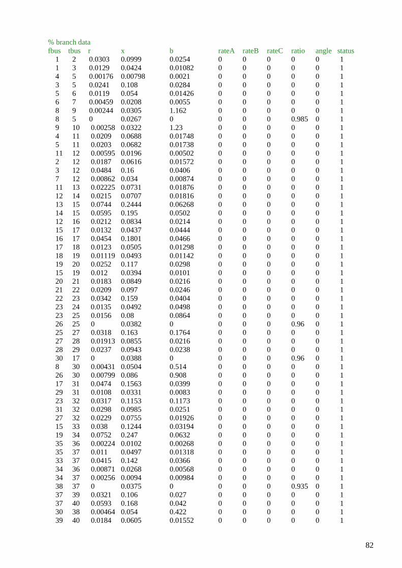
82
% branch data fbus tbus r x b rateA rateB rateC ratio angle status 1 2 0.0303 0.0999 0.0254 0 0 0 0 0 1 1 3 0.0129 0.0424 0.01082 0 0 0 0 0 1 4 5 0.00176 0.00798 0.0021 0 0 0 0 0 1 3 5 0.0241 0.108 0.0284 0 0 0 0 0 1 5 6 0.0119 0.054 0.01426 0 0 0 0 0 1 6 7 0.00459 0.0208 0.0055 0 0 0 0 0 1 8 9 0.00244 0.0305 1.162 0 0 0 0 0 1 8 5 0 0.0267 0 0 0 0 0.985 0 1 9 10 0.00258 0.0322 1.23 0 0 0 0 0 1 4 11 0.0209 0.0688 0.01748 0 0 0 0 0 1 5 11 0.0203 0.0682 0.01738 0 0 0 0 0 1 11 12 0.00595 0.0196 0.00502 0 0 0 0 0 1 2 12 0.0187 0.0616 0.01572 0 0 0 0 0 1 3 12 0.0484 0.16 0.0406 0 0 0 0 0 1 7 12 0.00862 0.034 0.00874 0 0 0 0 0 1 11 13 0.02225 0.0731 0.01876 0 0 0 0 0 1 12 14 0.0215 0.0707 0.01816 0 0 0 0 0 1 13 15 0.0744 0.2444 0.06268 0 0 0 0 0 1 14 15 0.0595 0.195 0.0502 0 0 0 0 0 1 12 16 0.0212 0.0834 0.0214 0 0 0 0 0 1 15 17 0.0132 0.0437 0.0444 0 0 0 0 0 1 16 17 0.0454 0.1801 0.0466 0 0 0 0 0 1 17 18 0.0123 0.0505 0.01298 0 0 0 0 0 1 18 19 0.01119 0.0493 0.01142 0 0 0 0 0 1 19 20 0.0252 0.117 0.0298 0 0 0 0 0 1 15 19 0.012 0.0394 0.0101 0 0 0 0 0 1 20 21 0.0183 0.0849 0.0216 0 0 0 0 0 1 21 22 0.0209 0.097 0.0246 0 0 0 0 0 1 22 23 0.0342 0.159 0.0404 0 0 0 0 0 1 23 24 0.0135 0.0492 0.0498 0 0 0 0 0 1 23 25 0.0156 0.08 0.0864 0 0 0 0 0 1 26 25 0 0.0382 0 0 0 0 0.96 0 1 25 27 0.0318 0.163 0.1764 0 0 0 0 0 1 27 28 0.01913 0.0855 0.0216 0 0 0 0 0 1 28 29 0.0237 0.0943 0.0238 0 0 0 0 0 1 30 17 0 0.0388 0 0 0 0 0.96 0 1 8 30 0.00431 0.0504 0.514 0 0 0 0 0 1 26 30 0.00799 0.086 0.908 0 0 0 0 0 1 17 31 0.0474 0.1563 0.0399 0 0 0 0 0 1 29 31 0.0108 0.0331 0.0083 0 0 0 0 0 1 23 32 0.0317 0.1153 0.1173 0 0 0 0 0 1 31 32 0.0298 0.0985 0.0251 0 0 0 0 0 1 27 32 0.0229 0.0755 0.01926 0 0 0 0 0 1 15 33 0.038 0.1244 0.03194 0 0 0 0 0 1 19 34 0.0752 0.247 0.0632 0 0 0 0 0 1 35 36 0.00224 0.0102 0.00268 0 0 0 0 0 1 35 37 0.011 0.0497 0.01318 0 0 0 0 0 1 33 37 0.0415 0.142 0.0366 0 0 0 0 0 1 34 36 0.00871 0.0268 0.00568 0 0 0 0 0 1 34 37 0.00256 0.0094 0.00984 0 0 0 0 0 1 38 37 0 0.0375 0 0 0 0 0.935 0 1 37 39 0.0321 0.106 0.027 0 0 0 0 0 1 37 40 0.0593 0.168 0.042 0 0 0 0 0 1 30 38 0.00464 0.054 0.422 0 0 0 0 0 1 39 40 0.0184 0.0605 0.01552 0 0 0 0 0 1
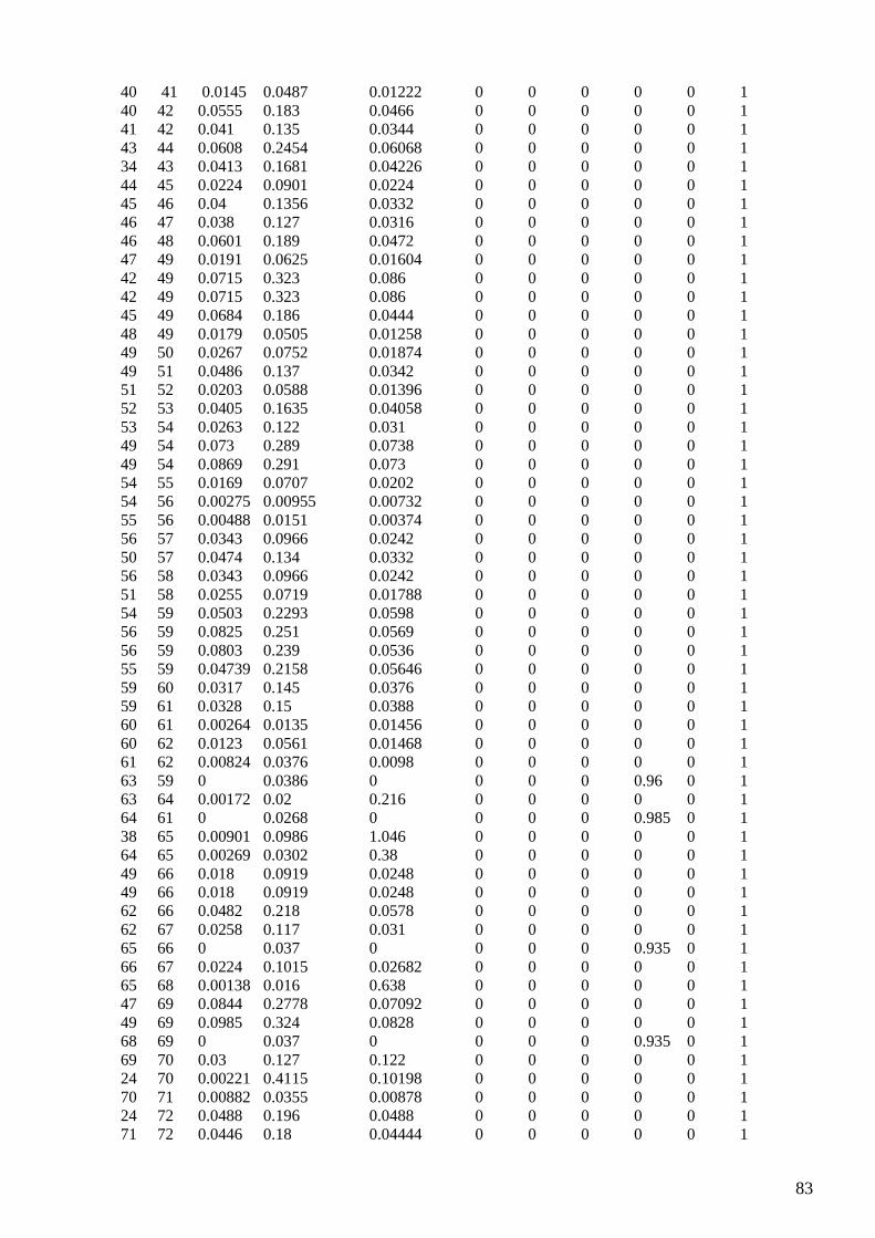
83
40 41 0.0145 0.0487 0.01222 0 0 0 0 0 1 40 42 0.0555 0.183 0.0466 0 0 0 0 0 1 41 42 0.041 0.135 0.0344 0 0 0 0 0 1 43 44 0.0608 0.2454 0.06068 0 0 0 0 0 1 34 43 0.0413 0.1681 0.04226 0 0 0 0 0 1 44 45 0.0224 0.0901 0.0224 0 0 0 0 0 1 45 46 0.04 0.1356 0.0332 0 0 0 0 0 1 46 47 0.038 0.127 0.0316 0 0 0 0 0 1 46 48 0.0601 0.189 0.0472 0 0 0 0 0 1 47 49 0.0191 0.0625 0.01604 0 0 0 0 0 1 42 49 0.0715 0.323 0.086 0 0 0 0 0 1 42 49 0.0715 0.323 0.086 0 0 0 0 0 1 45 49 0.0684 0.186 0.0444 0 0 0 0 0 1 48 49 0.0179 0.0505 0.01258 0 0 0 0 0 1 49 50 0.0267 0.0752 0.01874 0 0 0 0 0 1 49 51 0.0486 0.137 0.0342 0 0 0 0 0 1 51 52 0.0203 0.0588 0.01396 0 0 0 0 0 1 52 53 0.0405 0.1635 0.04058 0 0 0 0 0 1 53 54 0.0263 0.122 0.031 0 0 0 0 0 1 49 54 0.073 0.289 0.0738 0 0 0 0 0 1 49 54 0.0869 0.291 0.073 0 0 0 0 0 1 54 55 0.0169 0.0707 0.0202 0 0 0 0 0 1 54 56 0.00275 0.00955 0.00732 0 0 0 0 0 1 55 56 0.00488 0.0151 0.00374 0 0 0 0 0 1 56 57 0.0343 0.0966 0.0242 0 0 0 0 0 1 50 57 0.0474 0.134 0.0332 0 0 0 0 0 1 56 58 0.0343 0.0966 0.0242 0 0 0 0 0 1 51 58 0.0255 0.0719 0.01788 0 0 0 0 0 1 54 59 0.0503 0.2293 0.0598 0 0 0 0 0 1 56 59 0.0825 0.251 0.0569 0 0 0 0 0 1 56 59 0.0803 0.239 0.0536 0 0 0 0 0 1 55 59 0.04739 0.2158 0.05646 0 0 0 0 0 1 59 60 0.0317 0.145 0.0376 0 0 0 0 0 1 59 61 0.0328 0.15 0.0388 0 0 0 0 0 1 60 61 0.00264 0.0135 0.01456 0 0 0 0 0 1 60 62 0.0123 0.0561 0.01468 0 0 0 0 0 1 61 62 0.00824 0.0376 0.0098 0 0 0 0 0 1 63 59 0 0.0386 0 0 0 0 0.96 0 1 63 64 0.00172 0.02 0.216 0 0 0 0 0 1 64 61 0 0.0268 0 0 0 0 0.985 0 1 38 65 0.00901 0.0986 1.046 0 0 0 0 0 1 64 65 0.00269 0.0302 0.38 0 0 0 0 0 1 49 66 0.018 0.0919 0.0248 0 0 0 0 0 1 49 66 0.018 0.0919 0.0248 0 0 0 0 0 1 62 66 0.0482 0.218 0.0578 0 0 0 0 0 1 62 67 0.0258 0.117 0.031 0 0 0 0 0 1 65 66 0 0.037 0 0 0 0 0.935 0 1 66 67 0.0224 0.1015 0.02682 0 0 0 0 0 1 65 68 0.00138 0.016 0.638 0 0 0 0 0 1 47 69 0.0844 0.2778 0.07092 0 0 0 0 0 1 49 69 0.0985 0.324 0.0828 0 0 0 0 0 1 68 69 0 0.037 0 0 0 0 0.935 0 1 69 70 0.03 0.127 0.122 0 0 0 0 0 1 24 70 0.00221 0.4115 0.10198 0 0 0 0 0 1 70 71 0.00882 0.0355 0.00878 0 0 0 0 0 1 24 72 0.0488 0.196 0.0488 0 0 0 0 0 1 71 72 0.0446 0.18 0.04444 0 0 0 0 0 1

84
71 73 0.00866 0.0454 0.01178 0 0 0 0 0 1 70 74 0.0401 0.1323 0.03368 0 0 0 0 0 1 70 75 0.0428 0.141 0.036 0 0 0 0 0 1 69 75 0.0405 0.122 0.124 0 0 0 0 0 1 74 75 0.0123 0.0406 0.01034 0 0 0 0 0 1 76 77 0.0444 0.148 0.0368 0 0 0 0 0 1 69 77 0.0309 0.101 0.1038 0 0 0 0 0 1 75 77 0.0601 0.1999 0.04978 0 0 0 0 0 1 77 78 0.00376 0.0124 0.01264 0 0 0 0 0 1 78 79 0.00546 0.0244 0.00648 0 0 0 0 0 1 77 80 0.017 0.0485 0.0472 0 0 0 0 0 1 77 80 0.0294 0.105 0.0228 0 0 0 0 0 1 79 80 0.0156 0.0704 0.0187 0 0 0 0 0 1 68 81 0.00175 0.0202 0.808 0 0 0 0 0 1 81 80 0 0.037 0 0 0 0 0.935 0 1 77 82 0.0298 0.0853 0.08174 0 0 0 0 0 1 82 83 0.0112 0.03665 0.03796 0 0 0 0 0 1 83 84 0.0625 0.132 0.0258 0 0 0 0 0 1 83 85 0.043 0.148 0.0348 0 0 0 0 0 1 84 85 0.0302 0.0641 0.01234 0 0 0 0 0 1 85 86 0.035 0.123 0.0276 0 0 0 0 0 1 86 87 0.02828 0.2074 0.0445 0 0 0 0 0 1 85 88 0.02 0.102 0.0276 0 0 0 0 0 1 85 89 0.0239 0.173 0.047 0 0 0 0 0 1 88 89 0.0139 0.0712 0.01934 0 0 0 0 0 1 89 90 0.0518 0.188 0.0528 0 0 0 0 0 1 89 90 0.0238 0.0997 0.106 0 0 0 0 0 1 90 91 0.0254 0.0836 0.0214 0 0 0 0 0 1 89 92 0.0099 .0505 0.0548 0 0 0 0 0 1 89 92 0.0393 0.1581 0.0414 0 0 0 0 0 1 91 92 0.0387 0.1272 0.03268 0 0 0 0 0 1 92 93 0.0258 0.0848 0.0218 0 0 0 0 0 1 92 94 0.0481 0.158 0.0406 0 0 0 0 0 1 93 94 0.0223 0.0732 0.01876 0 0 0 0 0 1 94 95 0.0132 0.0434 0.0111 0 0 0 0 0 1 80 96 0.0356 0.182 0.0494 0 0 0 0 0 1 82 96 0.0162 0.053 0.0544 0 0 0 0 0 1 94 96 0.0269 0.0869 0.023 0 0 0 0 0 1 80 97 0.0183 0.0934 0.0254 0 0 0 0 0 1 80 98 0.0238 0.108 0.0286 0 0 0 0 0 1 80 99 0.0454 0.206 0.0546 0 0 0 0 0 1 92 100 0.0648 0.295 0.0472 0 0 0 0 0 1 94 100 0.0178 0.058 0.0604 0 0 0 0 0 1 95 96 0.0171 0.0547 0.01474 0 0 0 0 0 1 96 97 0.0173 0.0885 0.024 0 0 0 0 0 1 98 100 0.0397 0.179 0.0476 0 0 0 0 0 1 99 100 0.018 0.0813 0.0216 0 0 0 0 0 1 100 101 0.0277 0.1262 0.0328 0 0 0 0 0 1 92 102 0.0123 0.0559 0.01464 0 0 0 0 0 1 101 102 0.0246 0.112 0.0294 0 0 0 0 0 1 100 103 0.016 0.0525 0.0536 0 0 0 0 0 1 100 104 0.0451 0.204 0.0541 0 0 0 0 0 1 103 104 0.0466 0.1584 0.0407 0 0 0 0 0 1 103 105 0.0535 0.1625 0.0408 0 0 0 0 0 1 100 106 0.0605 0.229 0.062 0 0 0 0 0 1 104 105 0.00994 0.0378 0.00986 0 0 0 0 0 1 105 106 0.014 0.0547 0.01434 0 0 0 0 0 1
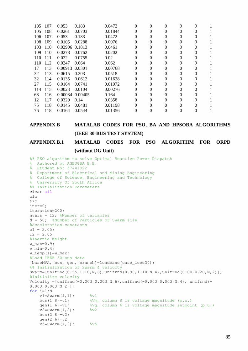
85
105 107 0.053 0.183 0.0472 0 0 0 0 0 1 105 108 0.0261 0.0703 0.01844 0 0 0 0 0 1 106 107 0.053 0.183 0.0472 0 0 0 0 0 1 108 109 0.0105 0.0288 0.0076 0 0 0 0 0 1 103 110 0.03906 0.1813 0.0461 0 0 0 0 0 1 109 110 0.0278 0.0762 0.0202 0 0 0 0 0 1 110 111 0.022 0.0755 0.02 0 0 0 0 0 1 110 112 0.0247 0.064 0.062 0 0 0 0 0 1 17 113 0.00913 0.0301 0.00768 0 0 0 0 0 1 32 113 0.0615 0.203 0.0518 0 0 0 0 0 1 32 114 0.0135 0.0612 0.01628 0 0 0 0 0 1 27 115 0.0164 0.0741 0.01972 0 0 0 0 0 1 114 115 0.0023 0.0104 0.00276 0 0 0 0 0 1 68 116 0.00034 0.00405 0.164 0 0 0 0 0 1 12 117 0.0329 0.14 0.0358 0 0 0 0 0 1 75 118 0.0145 0.0481 0.01198 0 0 0 0 0 1 76 118 0.0164 0.0544 0.01356 0 0 0 0 0 1
APPENDIX B MATALAB CODES FOR PSO, BA AND HPSOBA ALGORITHMS
(IEEE 30-BUS TEST SYSTEM)
APPENDIX B.1 MATALAB CODES FOR PSO ALGORITHM FOR ORPD
(without DG Unit)
%% PSO algorithm to solve Optimal Reactive Power Di spatch % Authored by AGBUGBA E.E. % Student No: 57441022 % Department of Electrical and Mining Engineering % College of Science, Engineering and Technology % University Of South Africa %% Initialization Parameters clear all clc tic iter=0; iteration=200; nvars = 12; %Number of variables N = 50; %Number of Particles or Swarm size %Acceleration constants c1 = 2.05; c2 = 2.05; %Inertia Weight w_max=0.9; w_min=0.4; w_temp(1)=w_max; %Load IEEE 30-bus data [baseMVA, bus, gen, branch]=loadcase(case_ieee30); %% Initialization of Swarm & velocity Swarm=[unifrnd(0.95,1.10,N,6),unifrnd(0.90,1.10,N,4 ),unifrnd(0.00,0.20,N,2)]; %Initialize velocity Velocity =[unifrnd(-0.003,0.003,N,6),unifrnd(-0.003 ,0.003,N,4), unifrnd(-0.003,0.003,N,2)]; for i=1:N v1=Swarm(i,1); %v1 bus(1,8)=v1; %Vm, column 8 is voltage magnitude (p.u.) gen(1,6)=v1; %Vg, column 6 is voltage magnitude setpoint (p.u.) v2=Swarm(i,2); %v2 bus(2,8)=v2; gen(2,6)=v2; v5=Swarm(i,3); %v5
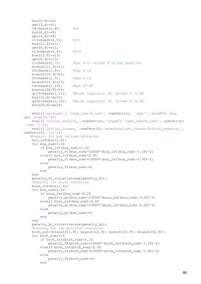
86
bus(5,8)=v5; gen(3,6)=v5; v8=Swarm(i,4); %v8 bus(8,8)=v8; gen(4,6)=v8; v11=Swarm(i,5); %v11 bus(11,8)=v11; gen(5,6)=v11; v13=Swarm(i,6); %v13 bus(13,8)=v13; gen(6,6)=v13; t1=Swarm(i,7); %tp1 6-9, column 9 is tap position branch(11,9)=t1; t2=Swarm(i,8); %tp2 6-10 branch(12,9)=t2; t3=Swarm(i,9); %tp3 4-12 branch(15,9)=t3; t4=Swarm(i,10); %tp4 27-28 branch(36,9)=t4; qc10=Swarm(i,11); %Shunt capacitor 10, column 6 is BS bus(10,6)=qc10; qc24=Swarm(i,12); %Shunt capacitor 10, column 6 is BS bus(24,6)=qc24; eval([ 'savecase (''case_ieee30_test' , num2str(i), '.mat'', baseMVA, bus, gen, branch)' ]); eval([ 'initial_results_' ,num2str(i), '=runpf(''case_ieee30_test' , num2str(i) '.mat'')' ]); eval([ 'initial_losses_' ,num2str(i), '=sum(real(get_losses(initial_results_' , num2str(i), ')))' ]); %Penalty for bus voltage violation bus_inf=bus(:,8); for bus_num=1:30 if bus_inf(bus_num)>1.10 penalty_Vl(bus_num)=10000*(bus_inf(bus_ num)-1.10)^2; elseif bus_inf(bus_num)<0.95 penalty_Vl(bus_num)=10000*(bus_inf(bus_ num)-0.95)^2; else penalty_Vl(bus_num)=0; end end penalty_Vl_violation=sum(penalty_Vl); %Penalty for shunt violation buus_inf=bus(:,6); for bus_num=1:30 if buus_inf(bus_num)>0.20 penalty_Qc(bus_num)=10000*(buus_inf(bus _num)-0.20)^2; elseif buus_inf(bus_num)<0.00 penalty_Qc(bus_num)=10000*(buus_inf(bus _num)-0.00)^2; else penalty_Qc(bus_num)=0; end end penalty_Qc_violation=sum(penalty_Qc); %Penalty for tap position violation brch_inf=[branch(11,9); branch(12,9); branch(15 ,9); branch(36,9)]; for brch_num=1:4 if brch_inf(brch_num)>1.10 penalty_Tk(brch_num)=10000*(brch_inf(br ch_num)-1.10)^2; elseif brch_inf(brch_num)<0.90 penalty_Tk(brch_num)=10000*(brch_inf(br ch_num)-0.90)^2; else penalty_Tk(brch_num)=0; end

87
end penalty_Tk_violation=sum(penalty_Tk); %objective function=sum of active power losses of t he transmission lines losses(i)=eval([ 'initial_losses_' ,num2str(i)]); %sum of real power losses of all branches Obj_fun_initial(i)=losses(i)+penalty_Vl_violation+p enalty_Qc_violation+penalty_Tk_violation; %augumented objective function with penalty functio n end %% Initialize best position (Pbest) and global best postion (Gbest) matrix Pbest=Swarm; Val_Pbest=Obj_fun_initial; %finding best particle in initial population [Val_Gbest,m]=min(Val_Pbest); Gbest=Swarm(m,:); %used to keep track of the best particle ever Gbest_calc=repmat(Swarm(m,:),N,1); %% PSO LOOP figure( 'NumberTitle' , 'off' , 'Name' , 'PSO Algorithm Based Optimal Reactive Power Dispatch' ); title( 'ACTIVE POWER LOSS MINIMIZATION' ); ylabel( 'Total Active Power Loss (MW)' ); xlabel( 'Iteration Number' ); grid on; hold on for iter=1:iteration % Update the value of the inertia weight w if iter <= iteration w_temp(iter)=w_max + (((w_min-w_max)/iterati on)*iter); %Change inertia weight end %generate random numbers R1=rand(N,nvars); R2=rand(N,nvars); % constriction factor %2.05+2.05=4.1; %2/abs(2-4.1-sqrt(4.1*4.1-4*4.1))=0.729 %calculate velocity Velocity=(w_temp(iter)*Velocity+c1*R1.*(Pbest-S warm)+c2*R2.*(Gbest_calc-Swarm)); for v_iter=1:nvars if v_iter==nvars Outstep=Velocity(:,v_iter)>0.003; Velocity(find(Outstep),v_iter)=0.003; Outstep=Velocity(:,v_iter)<-0.003; Velocity(find(Outstep),v_iter)=-0.003; else Outstep=Velocity(:,v_iter)>0.01; Velocity(find(Outstep),v_iter)=0.01; Outstep=Velocity(:,v_iter)<-0.01; Velocity(find(Outstep),v_iter)=-0.01; end end %update positions of particles Swarm=Swarm+0.729*Velocity; %evaluate a new swarm for k=1:N v1=Swarm(k,1); %v1 bus(1,8)=v1; %Vm, column 8 is voltage magnitude (p.u.) gen(1,6)=v1; %Vg, column 6 is voltage magnitude setpoint (p.u.) v2=Swarm(k,2); %v2 bus(2,8)=v2; gen(2,6)=v2; v5=Swarm(k,3); %v5 bus(5,8)=v5; gen(3,6)=v5;

88
v8=Swarm(k,4); %v8 bus(8,8)=v8; gen(4,6)=v8; v11=Swarm(k,5); %v11 bus(11,8)=v11; gen(5,6)=v11; v13=Swarm(k,6); %v13 bus(13,8)=v13; gen(6,6)=v13; t1=Swarm(k,7); %tp1 6-9, column 9 is tap position branch(11,9)=t1; t2=Swarm(k,8); %tp2 6-10 branch(12,9)=t2; t3=Swarm(k,9); %tp3 4-12 branch(15,9)=t3; t4=Swarm(k,10); %tp4 27-28 branch(36,9)=t4; qc10=Swarm(k,11); %Shunt capacitor 10, column 6 is BS bus(10,6)=qc10; qc24=Swarm(k,12); %Shunt capacitor 10, column 6 is BS bus(24,6)=qc24; eval([ 'savecase (''case_ieee30_test' , num2str(k), '.mat'', baseMVA, bus, gen, branch)' ]); eval([ 'final_results_' ,num2str(k), '=runpf(''case_ieee30_test' , num2str(k) '.mat'')' ]); eval([ 'final_losses_' ,num2str(k), '=sum(real(get_losses(final_results_' ,num2str(k), ')))' ]); %Penalty for bus voltage violation bus_inf=bus(:,8); for bus_num=1:30 if bus_inf(bus_num)>1.10 penalty_Vl(bus_num)=10000*(bus_inf( bus_num)-1.10)^2; elseif bus_inf(bus_num)<0.95 penalty_Vl(bus_num)=10000*(bus_inf( bus_num)-0.95)^2; else penalty_Vl(bus_num)=0; end end penalty_Vl_violation=sum(penalty_Vl); %Penalty for shunt violation buus_inf=bus(:,6); for bus_num=1:30 if buus_inf(bus_num)>0.20 penalty_Qc(bus_num)=10000*(buus_inf (bus_num)-0.20)^2; elseif buus_inf(bus_num)<0.00 penalty_Qc(bus_num)=10000*(buus_inf (bus_num)-0.00)^2; else penalty_Qc(bus_num)=0; end end penalty_Qc_violation=sum(penalty_Qc); %Penalty for tap position violation brch_inf=[branch(11,9); branch(12,9); branc h(15,9); branch(36,9)]; for brch_num=1:4 if brch_inf(brch_num)>1.10 penalty_Tk(brch_num)=10000*(brch_in f(brch_num)-1.10)^2; elseif brch_inf(brch_num)<0.90 penalty_Tk(brch_num)=10000*(brch_in f(brch_num)-0.90)^2; else penalty_Tk(brch_num)=0; end end
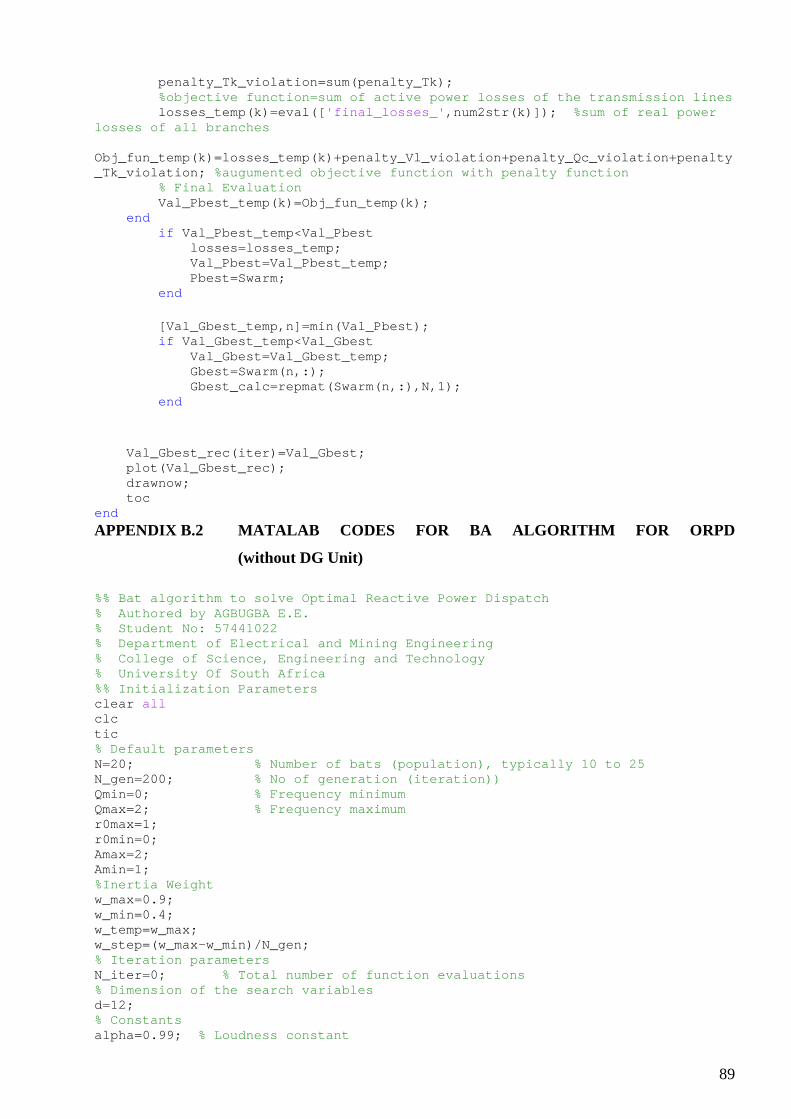
89
penalty_Tk_violation=sum(penalty_Tk); %objective function=sum of active power losses of t he transmission lines losses_temp(k)=eval([ 'final_losses_' ,num2str(k)]); %sum of real power losses of all branches Obj_fun_temp(k)=losses_temp(k)+penalty_Vl_violation +penalty_Qc_violation+penalty_Tk_violation; %augumented objective function with penalty functio n % Final Evaluation Val_Pbest_temp(k)=Obj_fun_temp(k); end if Val_Pbest_temp<Val_Pbest losses=losses_temp; Val_Pbest=Val_Pbest_temp; Pbest=Swarm; end [Val_Gbest_temp,n]=min(Val_Pbest); if Val_Gbest_temp<Val_Gbest Val_Gbest=Val_Gbest_temp; Gbest=Swarm(n,:); Gbest_calc=repmat(Swarm(n,:),N,1); end Val_Gbest_rec(iter)=Val_Gbest; plot(Val_Gbest_rec); drawnow; toc end APPENDIX B.2 MATALAB CODES FOR BA ALGORITHM FOR ORPD
(without DG Unit)
%% Bat algorithm to solve Optimal Reactive Power Di spatch % Authored by AGBUGBA E.E. % Student No: 57441022 % Department of Electrical and Mining Engineering % College of Science, Engineering and Technology % University Of South Africa %% Initialization Parameters clear all clc tic % Default parameters N=20; % Number of bats (population), typically 10 to 25 N_gen=200; % No of generation (iteration)) Qmin=0; % Frequency minimum Qmax=2; % Frequency maximum r0max=1; r0min=0; Amax=2; Amin=1; %Inertia Weight w_max=0.9; w_min=0.4; w_temp=w_max; w_step=(w_max-w_min)/N_gen; % Iteration parameters N_iter=0; % Total number of function evaluations % Dimension of the search variables d=12; % Constants alpha=0.99; % Loudness constant

90
gamma=0.9; % Pulse rate constant %Load IEEE 30-bus data [baseMVA, bus, gen, branch]=loadcase(case_ieee30); %% Initialization of Population/ Solutions, Frequen cy & velocity % Initialize velocity Velocity =[unifrnd(-0.003,0.003,N,6),unifrnd(-0.003 ,0.003,N,4), unifrnd(-0.003,0.003,N,2)]; % Initialize frequency Freq=zeros(N,1); % Frequency; % Initialize solutions/locations Sol=[unifrnd(0.95,1.10,N,6),unifrnd(0.90,1.10,N,4), unifrnd(0,0.20,N,2)]; r=(rand(N,1).*(r0max-r0min))+r0min; A=(rand(N,1).*(Amax-Amin))+Amin; for i=1:N v1=Sol(i,1); %v1 bus(1,8)=v1; %Vm, column 8 is voltage magnitude (p.u.) gen(1,6)=v1; %Vg, column 6 is voltage magnitude setpoint (p.u.) v2=Sol(i,2); %v2 bus(2,8)=v2; gen(2,6)=v2; v5=Sol(i,3); %v5 bus(5,8)=v5; gen(3,6)=v5; v8=Sol(i,4); %v8 bus(8,8)=v8; gen(4,6)=v8; v11=Sol(i,5); %v11 bus(11,8)=v11; gen(5,6)=v11; v13=Sol(i,6); %v13 bus(13,8)=v13; gen(6,6)=v13; t1=Sol(i,7); %tp1 6-9, column 9 is tap position branch(11,9)=t1; t2=Sol(i,8); %tp2 6-10 branch(12,9)=t2; t3=Sol(i,9); %tp3 4-12 branch(15,9)=t3; t4=Sol(i,10); %tp4 27-28 branch(36,9)=t4; qc10=Sol(i,11); %Shunt capacitor 10, column 6 is BS bus(10,6)=qc10; qc24=Sol(i,12); %Shunt capacitor 10, column 6 is BS bus(24,6)=qc24; eval([ 'savecase (''2case_ieee30_test' , num2str(i), '.mat'', baseMVA, bus, gen, branch)' ]); eval([ 'results_' ,num2str(i), '=runpf(''2case_ieee30_test' , num2str(i) '.mat'')' ]); eval([ 'losses_' ,num2str(i), '=sum(real(get_losses(results_' ,num2str(i), ')))' ]); %Penalty for bus voltage violation bus_inf=bus(:,8); for bus_num=1:30 if bus_inf(bus_num)>1.10 penalty_bus(bus_num)=10000*((bus_inf(bu s_num)-1.10)^2); elseif bus_inf(bus_num)<0.95 penalty_bus(bus_num)=10000*((bus_inf(bu s_num)-0.95)^2); else penalty_bus(bus_num)=0; end end penalty_bus_violation=sum(penalty_bus); %Penalty for shunt violation
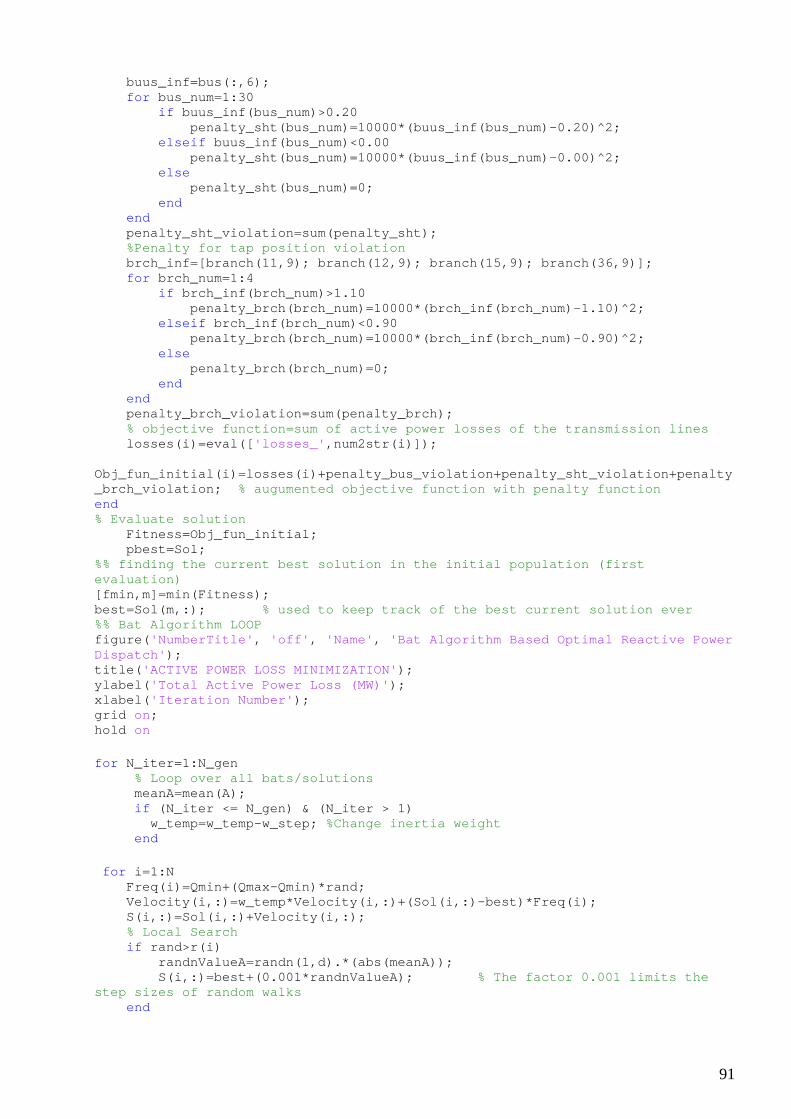
91
buus_inf=bus(:,6); for bus_num=1:30 if buus_inf(bus_num)>0.20 penalty_sht(bus_num)=10000*(buus_inf(bu s_num)-0.20)^2; elseif buus_inf(bus_num)<0.00 penalty_sht(bus_num)=10000*(buus_inf(bu s_num)-0.00)^2; else penalty_sht(bus_num)=0; end end penalty_sht_violation=sum(penalty_sht); %Penalty for tap position violation brch_inf=[branch(11,9); branch(12,9); branch(15 ,9); branch(36,9)]; for brch_num=1:4 if brch_inf(brch_num)>1.10 penalty_brch(brch_num)=10000*(brch_inf( brch_num)-1.10)^2; elseif brch_inf(brch_num)<0.90 penalty_brch(brch_num)=10000*(brch_inf( brch_num)-0.90)^2; else penalty_brch(brch_num)=0; end end penalty_brch_violation=sum(penalty_brch); % objective function=sum of active power losses of the transmission lines losses(i)=eval([ 'losses_' ,num2str(i)]); Obj_fun_initial(i)=losses(i)+penalty_bus_violation+ penalty_sht_violation+penalty_brch_violation; % augumented objective function with penalty functi on end % Evaluate solution Fitness=Obj_fun_initial; pbest=Sol; %% finding the current best solution in the initial population (first evaluation) [fmin,m]=min(Fitness); best=Sol(m,:); % used to keep track of the best current solution e ver %% Bat Algorithm LOOP figure( 'NumberTitle' , 'off' , 'Name' , 'Bat Algorithm Based Optimal Reactive Power Dispatch' ); title( 'ACTIVE POWER LOSS MINIMIZATION' ); ylabel( 'Total Active Power Loss (MW)' ); xlabel( 'Iteration Number' ); grid on; hold on for N_iter=1:N_gen % Loop over all bats/solutions meanA=mean(A); if (N_iter <= N_gen) & (N_iter > 1) w_temp=w_temp-w_step; %Change inertia weight end for i=1:N Freq(i)=Qmin+(Qmax-Qmin)*rand; Velocity(i,:)=w_temp*Velocity(i,:)+(Sol(i,:)-be st)*Freq(i); S(i,:)=Sol(i,:)+Velocity(i,:); % Local Search if rand>r(i) randnValueA=randn(1,d).*(abs(meanA)); S(i,:)=best+(0.001*randnValueA); % The factor 0.001 limits the step sizes of random walks end
92
v1=S(i,1); %v1 bus(1,8)=v1; %Vm, column 8 is voltage magnitude (p.u.) gen(1,6)=v1; %Vg, column 6 is voltage magnitude setpoint (p.u.) v2=S(i,2); %v2 bus(2,8)=v2; gen(2,6)=v2; v5=S(i,3); %v5 bus(5,8)=v5; gen(3,6)=v5; v8=S(i,4); %v8 bus(8,8)=v8; gen(4,6)=v8; v11=S(i,5); %v11 bus(11,8)=v11; gen(5,6)=v11; v13=S(i,6); %v13 bus(13,8)=v13; gen(6,6)=v13; t1=S(i,7); %tp1 6-9, column 9 is tap position branch(11,9)=t1; t2=S(i,8); %tp2 6-10 branch(12,9)=t2; t3=S(i,9); %tp3 4-12 branch(15,9)=t3; t4=S(i,10); %tp4 27-28 branch(36,9)=t4; qc10=S(i,11); %Shunt capacitor 10, column 6 is BS bus(10,6)=qc10; qc24=S(i,12); %Shunt capacitor 10, column 6 is BS bus(24,6)=qc24; eval([ 'savecase (''2case_ieee30_test' , num2str(i), '.mat'', baseMVA, bus, gen, branch)' ]); eval([ 'results_' ,num2str(i), '=runpf(''2case_ieee30_test' , num2str(i) '.mat'')' ]); eval([ 'losses_' ,num2str(i), '=sum(real(get_losses(results_' ,num2str(i), ')))' ]); %Penalty for bus voltage violation bus_inf=bus(:,8); for bus_num=1:30 if bus_inf(bus_num)>1.10 penalty_bus(bus_num)=10000*((bus_inf(bu s_num)-1.10)^2); elseif bus_inf(bus_num)<0.95 penalty_bus(bus_num)=10000*((bus_inf(bu s_num)-0.95)^2); else penalty_bus(bus_num)=0; end end penalty_bus_violation=sum(penalty_bus); %Penalty for shunt violation buus_inf=bus(:,6); for bus_num=1:30 if buus_inf(bus_num)>0.20 penalty_sht(bus_num)=10000*(buus_inf(bu s_num)-0.20)^2; elseif buus_inf(bus_num)<0.00 penalty_sht(bus_num)=10000*(buus_inf(bu s_num)-0.00)^2; else penalty_sht(bus_num)=0; end end penalty_sht_violation=sum(penalty_sht);

93
%Penalty for tap position violation brch_inf=[branch(11,9); branch(12,9); branch(15 ,9); branch(36,9)]; for brch_num=1:4 if brch_inf(brch_num)>1.10 penalty_brch(brch_num)=10000*(brch_inf( brch_num)-1.10)^2; elseif brch_inf(brch_num)<0.90 penalty_brch(brch_num)=10000*(brch_inf( brch_num)-0.90)^2; else penalty_brch(brch_num)=0; end end penalty_brch_violation=sum(penalty_brch); %sum of real power losses of all branches losses_final(i)=eval([ 'losses_' ,num2str(i)]); Obj_fun_final(i)=losses_final(i)+penalty_bus_violat ion+penalty_sht_violation+penalty_brch_violation; % Evaluate new solutions Fitness_final(i)=Obj_fun_final(i); %% If the solution improves or not too loud if (Fitness_final(i)<=Fitness(i)) & (rand<A(i)) losses(i)=losses_final(i); Sol(i,:)=S(i,:); % replace initial solution with improved solution Fitness(i)=Fitness_final(i); % replace initial FITNESS with improved fitness A(i)=A(i)*alpha; % update loudness of bats r(i)=r(i)*(1-exp(-gamma*N_iter)); % update the pitch of bats end [fnew,n]=min(Fitness_final); % Update the current best if fnew<=fmin best=S(n,:); fmin=fnew; end end fmin_rec(N_iter)=fmin; plot(fmin_rec); drawnow; toc end
APPENDIX B.3 MATALAB CODES FOR HPSOBA ALGORITHM FOR ORPD
(without DG Unit)
%% Hybrid PSO-BA algorithm to solve Optimal Reactiv e Power Dispatch % Authored by AGBUGBA E.E. % Student No: 57441022 % Department of Electrical and Mining Engineering % College of Science, Engineering and Technology % University Of South Africa %% Initialization Parameters clear all clc tic % Dimension of the search variables d=12; % Bat Algorithm Default parameters

94
N=20; % Number of bats (population), typically 10 to 25 N_gen=200; % No of generation (iteration) Q_max=2; % Frequency maximum Q_min=0; % Frequency minimum r_max=1; % Maximum pulse rate r_min=0; % Minimum pulse rate A_max=2; % Maximum loudness A_min=1; % Minimum loudness % Constants alpha=0.99; % Loudness constant gamma=0.9; % Pulse rate constant % PSO Algorithm Default parameters % Inertia Weight w_max=0.9; w_min=0.4; w_temp(1)=w_max; % Acceleration constants c1=2.05; c2=2.05; % Iteration parameters N_iter=0; %Load IEEE 30-bus data [baseMVA, bus, gen, branch]=loadcase(case_ieee30); %% Initialization of Population/ Solutions, Frequen cy & velocity % Initialize velocity Velocity =[unifrnd(-0.003,0.003,N,6),unifrnd(-0.003 ,0.003,N,4), unifrnd(-0.003,0.003,N,2)]; % Initialize frequency Freq=zeros(N,1); % Frequency; % Initialize solutions/locations Sol=[unifrnd(0.95,1.10,N,6),unifrnd(0.90,1.10,N,4), unifrnd(0,0.20,N,2)]; % Initialize pulse rate r=(rand(N,1).*(r_max-r_min))+r_min; % Initialize loudness A=(rand(N,1).*(A_max-A_min))+A_min; for i=1:N v1=Sol(i,1); %v1 bus(1,8)=v1; %Vm, column 8 is voltage magnitude (p.u.) gen(1,6)=v1; %Vg, column 6 is voltage magnitude setpoint (p.u.) v2=Sol(i,2); %v2 bus(2,8)=v2; gen(2,6)=v2; v5=Sol(i,3); %v5 bus(5,8)=v5; gen(3,6)=v5; v8=Sol(i,4); %v8 bus(8,8)=v8; gen(4,6)=v8; v11=Sol(i,5); %v11 bus(11,8)=v11; gen(5,6)=v11; v13=Sol(i,6); %v13 bus(13,8)=v13; gen(6,6)=v13; t1=Sol(i,7); %tp1 6-9, column 9 is tap position branch(11,9)=t1; t2=Sol(i,8); %tp2 6-10 branch(12,9)=t2; t3=Sol(i,9); %tp3 4-12

95
branch(15,9)=t3; t4=Sol(i,10); %tp4 27-28 branch(36,9)=t4; qc10=Sol(i,11); %Shunt capacitor 10, column 6 is BS bus(10,6)=qc10; qc24=Sol(i,12); %Shunt capacitor 10, column 6 is BS bus(24,6)=qc24; eval([ 'savecase (''2case_ieee30_test' , num2str(i), '.mat'', baseMVA, bus, gen, branch)' ]); eval([ 'results_' ,num2str(i), '=runpf(''2case_ieee30_test' , num2str(i) '.mat'')' ]); eval([ 'losses_' ,num2str(i), '=sum(real(get_losses(results_' ,num2str(i), ')))' ]); %Penalty for bus voltage violation bus_inf=bus(:,8); for bus_num=1:30 if bus_inf(bus_num)>1.10 penalty_bus(bus_num)=10000*(bus_inf(bus _num)-1.10)^2; elseif bus_inf(bus_num)<0.95 penalty_bus(bus_num)=10000*(bus_inf(bus _num)-0.95)^2; else penalty_bus(bus_num)=0; end end penalty_bus_violation=sum(penalty_bus); %Penalty for reactive shunt violation buus_inf=bus(:,6); for bus_num=1:30 if buus_inf(bus_num)>0.20 penalty_sht(bus_num)=10000*(buus_inf(bu s_num)-0.20)^2; elseif buus_inf(bus_num)<0.00 penalty_sht(bus_num)=10000*(buus_inf(bu s_num)-0.00)^2; else penalty_sht(bus_num)=0; end end penalty_sht_violation=sum(penalty_sht); %Penalty for tap position violation brch_inf=[branch(11,9); branch(12,9); branch(15 ,9); branch(36,9)]; for brch_num=1:4 if brch_inf(brch_num)>1.10 penalty_brch(brch_num)=10000*(brch_inf( brch_num)-1.10)^2; elseif brch_inf(brch_num)<0.90 penalty_brch(brch_num)=10000*(brch_inf( brch_num)-0.90)^2; else penalty_brch(brch_num)=0; end end penalty_brch_violation=sum(penalty_brch); % objective function=sum of active power losses of the transmission lines losses(i)=eval([ 'losses_' ,num2str(i)]); Obj_fun_initial(i)=losses(i)+penalty_bus_violation+ penalty_sht_violation+penalty_brch_violation; % augumented objective function with penalty functi on end % Evaluate solution Fitness=Obj_fun_initial; pbest=Sol; %% finding the current best solution in the initial population (first evaluation) [fmin,m]=min(Fitness);
96
best=Sol(m,:); % used to keep track of the best current solution e ver %% Hybrid PSO-BA Algorithm LOOP figure( 'NumberTitle' , 'off' , 'Name' , 'Hybrid PSO-BA Algorithm Based Optimal Reactive Power Dispatch' ); title( 'ACTIVE POWER LOSS MINIMIZATION' ); ylabel( 'Total Active Power Loss (MW)' ); xlabel( 'Iteration Number' ); grid on; hold on for N_iter=1:N_gen % Loop over all bats/particles meanA=mean(A); % Update the value of the inertia weight w if N_iter <= N_gen w_temp(N_iter)=w_max + (((w_min-w_max)/N_gen )*N_iter); %Change inertia weight end for k=1:N Freq(k)=Q_min+(Q_max-Q_min)*rand; Velocity(k,:)=w_temp(N_iter).*Velocity(k,:)+(c1 *rand*(pbest(k,:)-Sol(k,:))+c2*rand*(best-Sol(k,:)))*Freq(k); for v_iter=1:d if v_iter==d Outstep=Velocity(:,v_iter)>0.003; Velocity(find(Outstep),v_iter)=0.003; Outstep=Velocity(:,v_iter)<-0.003; Velocity(find(Outstep),v_iter)=-0.003; else Outstep=Velocity(:,v_iter)>0.01; Velocity(find(Outstep),v_iter)=0.01; Outstep=Velocity(:,v_iter)<-0.01; Velocity(find(Outstep),v_iter)=-0.01; end end Sol(k,:)=best+Velocity(k,:); % Local Search if rand>r(k) randnValueA=randn(1,d).*(abs(meanA)); Sol(k,:)=best+(0.001*randnValueA); % The factor 0.001 limits the step sizes of random walks end v1=Sol(k,1); %v1 bus(1,8)=v1; %Vm, column 8 is voltage magnitude (p.u.) gen(1,6)=v1; %Vg, column 6 is voltage magnitude setpoint (p.u.) v2=Sol(k,2); %v2 bus(2,8)=v2; gen(2,6)=v2; v5=Sol(k,3); %v5 bus(5,8)=v5; gen(3,6)=v5; v8=Sol(k,4); %v8 bus(8,8)=v8; gen(4,6)=v8; v11=Sol(k,5); %v11 bus(11,8)=v11; gen(5,6)=v11; v13=Sol(k,6); %v13 bus(13,8)=v13; gen(6,6)=v13; t1=Sol(k,7); %tp1 6-9, column 9 is tap position

97
branch(11,9)=t1; t2=Sol(k,8); %tp2 6-10 branch(12,9)=t2; t3=Sol(k,9); %tp3 4-12 branch(15,9)=t3; t4=Sol(k,10); %tp4 27-28 branch(36,9)=t4; qc10=Sol(k,11); %Shunt capacitor 10, column 6 is BS bus(10,6)=qc10; qc24=Sol(k,12); %Shunt capacitor 10, column 6 is BS bus(24,6)=qc24; eval([ 'savecase (''2case_ieee30_test' , num2str(k), '.mat'', baseMVA, bus, gen, branch)' ]); eval([ 'results_' ,num2str(k), '=runpf(''2case_ieee30_test' , num2str(k) '.mat'')' ]); eval([ 'losses_' ,num2str(k), '=sum(real(get_losses(results_' ,num2str(k), ')))' ]); %Penalty for bus voltage violation bus_inf=bus(:,8); for bus_num=1:30 if bus_inf(bus_num)>1.10 penalty_bus(bus_num)=10000*(bus_inf(bus _num)-1.10)^2; elseif bus_inf(bus_num)<0.95 penalty_bus(bus_num)=10000*(bus_inf(bus _num)-0.95)^2; else penalty_bus(bus_num)=0; end end penalty_bus_violation=sum(penalty_bus); %Penalty for reactive shunt violation buus_inf=bus(:,6); for bus_num=1:30 if buus_inf(bus_num)>0.20 penalty_sht(bus_num)=10000*(buus_inf(bu s_num)-0.20)^2; elseif buus_inf(bus_num)<0.00 penalty_sht(bus_num)=10000*(buus_inf(bu s_num)-0.00)^2; else penalty_sht(bus_num)=0; end end penalty_sht_violation=sum(penalty_sht); %Penalty for tap position violation brch_inf=[branch(11,9); branch(12,9); branch(15 ,9); branch(36,9)]; for brch_num=1:4 if brch_inf(brch_num)>1.10 penalty_brch(brch_num)=10000*(brch_inf( brch_num)-1.10)^2; elseif brch_inf(brch_num)<0.90 penalty_brch(brch_num)=10000*(brch_inf( brch_num)-0.90)^2; else penalty_brch(brch_num)=0; end end penalty_brch_violation=sum(penalty_brch); %sum of real power losses of all branches losses_final(k)=eval([ 'losses_' ,num2str(k)]); Obj_fun_final(k)=losses_final(k)+penalty_bus_violat ion+penalty_sht_violation+penalty_brch_violation; % Evaluate new solutions Fitness_final(k)=Obj_fun_final(k);

98
%% If the solution improves or not too loud if Fitness_final(k)<=Fitness(k) & (rand<A(k)) losses(k)=losses_final(k); pbest(k,:)=Sol(k,:); % replace initial solution with improved solution Fitness(k)=Fitness_final(k); % replace initial FITNESS with improved fitness A(k)=A(k)*alpha; % update loudness of bats r(k)=r(k)*(1-exp(-gamma*N_iter)); % update the pitch of bats end [fnew,n]=min(Fitness_final); % Update the current best if fnew<=fmin best=Sol(n,:); fmin=fnew; end end fmin_rec(N_iter)=fmin; plot(fmin_rec); drawnow; toc end APPENDIX C MATALAB CODES FOR PSO, BA AND HPSOBA ALGORITHMS
(IEEE 118-BUS TEST SYSTEM)
APPENDIX C.1 MATALAB CODES FOR PSO ALGORITHM FOR ORPD
(without DG Unit)
%% PSO algorithm to solve Optimal Reactive Power Di spatch % Authored by AGBUGBA E.E. % Student No: 57441022 % Department of Electrical and Mining Engineering % College of Science, Engineering and Technology % University Of South Africa %% Initialization Parameters clear all clc tic iter=0; iteration=200; nvars = 77; %Number of variables N = 50; %Number of Particles or Swarm size %Acceleration constants c1 = 2.05; c2 = 2.05; %Inertia Weight w_max=0.9; w_min=0.4; w_temp(1)=w_max; %Load IEEE 118-bus data [baseMVA, bus, gen, branch]=loadcase(case118); %% Initialization of Swarm & velocity % Random 50*77 matrix Swarm=[unifrnd(0.95,1.10,N,54),unifrnd(0.90,1.10,N, 9),unifrnd(0.00,0.25,N,14)]; %Initialize velocity Velocity =[unifrnd(-0.003,0.003,N,54),unifrnd(-0.00 3,0.003,N,9), unifrnd(-0.003,0.003,N,14)]; for i=1:N
99
v1=Swarm(i,1); %v1 bus(1,8)=v1; %Vm, column 8 is voltage magnitude (p.u.) gen(1,6)=v1; %Vg, column 6 is voltage magnitude setpoint (p.u.) v4=Swarm(i,2); %v4 bus(4,8)=v4; gen(2,6)=v4; v6=Swarm(i,3); %v6 bus(6,8)=v6; gen(3,6)=v6; v8=Swarm(i,4); %v8 bus(8,8)=v8; gen(4,6)=v8; v10=Swarm(i,5); %v10 bus(10,8)=v10; gen(5,6)=v10; v12=Swarm(i,6); %v12 bus(12,8)=v12; gen(6,6)=v12; v15=Swarm(i,7); %v15 bus(15,8)=v15; gen(7,6)=v15; v18=Swarm(i,8); %v18 bus(18,8)=v18; gen(8,6)=v18; v19=Swarm(i,9); %v19 bus(19,8)=v19; gen(9,6)=v19; v24=Swarm(i,10); %v24 bus(24,8)=v24; gen(10,6)=v24; v25=Swarm(i,11); %v25 bus(25,8)=v25; gen(11,6)=v25; v26=Swarm(i,12); %v26 bus(26,8)=v26; gen(12,6)=v26; v27=Swarm(i,13); %v27 bus(27,8)=v27; gen(13,6)=v27; v31=Swarm(i,14); %v31 bus(31,8)=v31; gen(14,6)=v31; v32=Swarm(i,15); %v32 bus(32,8)=v32; gen(15,6)=v32; v34=Swarm(i,16); %v34 bus(34,8)=v34; gen(16,6)=v34; v36=Swarm(i,17); %v36 bus(36,8)=v36; gen(17,6)=v36; v40=Swarm(i,18); %v40 bus(40,8)=v40; gen(18,6)=v40; v42=Swarm(i,19); %v42 bus(42,8)=v42; gen(19,6)=v42; v46=Swarm(i,20); %v46 bus(46,8)=v46; gen(20,6)=v46; v49=Swarm(i,21); %v49 bus(49,8)=v49; gen(21,6)=v49; v54=Swarm(i,22); %v54

100
bus(54,8)=v54; gen(22,6)=v54; v55=Swarm(i,23); %v55 bus(55,8)=v55; gen(23,6)=v55; v56=Swarm(i,24); %v56 bus(56,8)=v56; gen(24,6)=v56; v59=Swarm(i,25); %v59 bus(59,8)=v59; gen(25,6)=v59; v61=Swarm(i,26); %v61 bus(61,8)=v61; gen(26,6)=v61; v62=Swarm(i,27); %v62 bus(62,8)=v62; gen(27,6)=v62; v65=Swarm(i,28); %v65 bus(65,8)=v65; gen(28,6)=v65; v66=Swarm(i,29); %v66 bus(66,8)=v66; gen(29,6)=v66; v69=Swarm(i,30); %v69 bus(69,8)=v69; gen(30,6)=v69; v70=Swarm(i,31); %v70 bus(70,8)=v70; gen(31,6)=v70; v72=Swarm(i,32); %v72 bus(72,8)=v72; gen(32,6)=v72; v73=Swarm(i,33); %v73 bus(73,8)=v73; gen(33,6)=v73; v74=Swarm(i,34); %v74 bus(74,8)=v74; gen(34,6)=v74; v76=Swarm(i,35); %v76 bus(76,8)=v76; gen(35,6)=v76; v77=Swarm(i,36); %v77 bus(77,8)=v77; gen(36,6)=v77; v80=Swarm(i,37); %v80 bus(80,8)=v80; gen(37,6)=v80; v85=Swarm(i,38); %v85 bus(85,8)=v85; gen(38,6)=v85; v87=Swarm(i,39); %v87 bus(87,8)=v87; gen(39,6)=v87; v89=Swarm(i,40); %v89 bus(89,8)=v89; gen(40,6)=v89; v90=Swarm(i,41); %v90 bus(90,8)=v90; gen(41,6)=v90; v91=Swarm(i,42); %v91 bus(91,8)=v91; gen(42,6)=v91; v92=Swarm(i,43); %v92 bus(92,8)=v92;

101
gen(43,6)=v92; v99=Swarm(i,44); %v99 bus(99,8)=v99; gen(44,6)=v99; v100=Swarm(i,45); %v100 bus(100,8)=v100; gen(45,6)=v100; v103=Swarm(i,46); %v103 bus(103,8)=v103; gen(46,6)=v103; v104=Swarm(i,47); %v104 bus(104,8)=v104; gen(47,6)=v104; v105=Swarm(i,48); %v105 bus(105,8)=v105; gen(48,6)=v105; v107=Swarm(i,49); %v107 bus(107,8)=v107; gen(49,6)=v107; v110=Swarm(i,50); %v110 bus(110,8)=v110; gen(50,6)=v110; v111=Swarm(i,51); %v111 bus(111,8)=v111; gen(51,6)=v111; v112=Swarm(i,52); %v112 bus(112,8)=v112; gen(52,6)=v112; v113=Swarm(i,53); %v113 bus(113,8)=v113; gen(53,6)=v113; v116=Swarm(i,54); %v116 bus(116,8)=v116; gen(54,6)=v116; t1=Swarm(i,55); %tp1 8-5, column 9 is tap position branch(8,9)=t1; t2=Swarm(i,56); %tp2 26-25 branch(32,9)=t2; t3=Swarm(i,57); %tp3 30-17 branch(36,9)=t3; t4=Swarm(i,58); %tp4 38-37 branch(51,9)=t4; t5=Swarm(i,59); %tp5 63-59 branch(93,9)=t5; t6=Swarm(i,60); %tp6 64-61 branch(95,9)=t6; t7=Swarm(i,61); %tp7 65-66 branch(102,9)=t7; t8=Swarm(i,62); %tp8 68-69 branch(107,9)=t8; t9=Swarm(i,63); %tp9 81-80 branch(127,9)=t9; qc5=Swarm(i,64); %Shunt capacitor 5, column 6 is BS bus(5,6)=qc5; qc34=Swarm(i,65); %Shunt capacitor 34, column 6 is BS bus(34,6)=qc34; qc37=Swarm(i,66); %Shunt capacitor 37, column 6 is BS bus(37,6)=qc37; qc44=Swarm(i,67); %Shunt capacitor 44, column 6 is BS bus(44,6)=qc44; qc45=Swarm(i,68); %Shunt capacitor 45, column 6 is BS bus(45,6)=qc45; qc46=Swarm(i,69); %Shunt capacitor 46, column 6 is BS bus(46,6)=qc46;
102
qc48=Swarm(i,70); %Shunt capacitor 48, column 6 is BS bus(48,6)=qc48; qc74=Swarm(i,71); %Shunt capacitor 74, column 6 is BS bus(74,6)=qc74; qc79=Swarm(i,72); %Shunt capacitor 79, column 6 is BS bus(79,6)=qc79; qc82=Swarm(i,73); %Shunt capacitor 82, column 6 is BS bus(82,6)=qc82; qc83=Swarm(i,74); %Shunt capacitor 83, column 6 is BS bus(83,6)=qc83; qc105=Swarm(i,75); %Shunt capacitor 105, column 6 is BS bus(105,6)=qc105; qc107=Swarm(i,76); %Shunt capacitor 107, column 6 is BS bus(107,6)=qc107; qc110=Swarm(i,77); %Shunt capacitor 110, column 6 is BS bus(110,6)=qc110; eval([ 'savecase (''case118_test' , num2str(i), '.mat'', baseMVA, bus, gen, branch)' ]); eval([ 'initial_results_' ,num2str(i), '=runpf(''case118_test' , num2str(i) '.mat'')' ]); eval([ 'initial_losses_' ,num2str(i), '=sum(real(get_losses(initial_results_' , num2str(i), ')))' ]); %Penalty for bus voltage violation bus_inf=bus(:,8); for bus_num=1:118 if bus_inf(bus_num)>1.10 penalty_Vl(bus_num)=1000*(bus_inf(bus_n um)-1.10)^2; elseif bus_inf(bus_num)<0.95 penalty_Vl(bus_num)=1000*(bus_inf(bus_n um)-0.95)^2; else penalty_Vl(bus_num)=0; end end penalty_Vl_violation=sum(penalty_Vl); %Penalty for shunt violation buus_inf=bus(:,6); for bus_num=1:118 if buus_inf(bus_num)>0.25 penalty_Qc(bus_num)=1000*(buus_inf(bus_ num)-0.25)^2; elseif buus_inf(bus_num)<0.00 penalty_Qc(bus_num)=1000*(buus_inf(bus_ num)-0.00)^2; else penalty_Qc(bus_num)=0; end end penalty_Qc_violation=sum(penalty_Qc); %Penalty for tap position violation brch_inf=[branch(8,9); branch(32,9); branch(36, 9); branch(51,9); branch(93,9); branch(95,9); branch(102,9); branch(1 07,9); branch(127,9)]; for brch_num=1:9 if brch_inf(brch_num)>1.10 penalty_Tk(brch_num)=1000*(brch_inf(brc h_num)-1.10)^2; elseif brch_inf(brch_num)<0.90 penalty_Tk(brch_num)=1000*(brch_inf(brc h_num)-0.90)^2; else penalty_Tk(brch_num)=0; end end penalty_Tk_violation=sum(penalty_Tk); %objective function=sum of active power losses of t he transmission lines

103
losses(i)=eval([ 'initial_losses_' ,num2str(i)]); %sum of real power losses of all branches Obj_fun_initial(i)=losses(i)+penalty_Vl_violation+p enalty_Qc_violation+penalty_Tk_violation; %augumented objective function with penalty functio n end %% Initialize best position (Pbest) and global best postion (Gbest) matrix Pbest=Swarm; Val_Pbest=Obj_fun_initial; %finding best particle in initial population [Val_Gbest,m]=min(Val_Pbest); Gbest=Swarm(m,:); %used to keep track of the best particle ever Gbest_calc=repmat(Swarm(m,:),N,1); %% PSO LOOP figure( 'NumberTitle' , 'off' , 'Name' , 'PSO Algorithm Based Optimal Reactive Power Dispatch' ); title( 'ACTIVE POWER LOSS MINIMIZATION' ); ylabel( 'Total Active Power Loss (MW)' ); xlabel( 'Iteration Number' ); grid on; hold on for iter=1:iteration % Update the value of the inertia weight w if iter <= iteration w_temp(iter)=w_max + (((w_min-w_max)/iterati on)*iter); %Change inertia weight end %generate random numbers R1=rand(N,nvars); R2=rand(N,nvars); % constriction factor %2.05+2.05=4.1; %2/abs(2-4.1-sqrt(4.1*4.1-4*4.1))=0.729 %calculate velocity Velocity=(w_temp(iter).*Velocity+c1*R1.*(Pbest- Swarm)+c2*R2.*(Gbest_calc-Swarm)); for v_iter=1:nvars if v_iter==nvars Outstep=Velocity(:,v_iter)>0.003; Velocity(find(Outstep),v_iter)=0.003; Outstep=Velocity(:,v_iter)<-0.003; Velocity(find(Outstep),v_iter)=-0.003; else Outstep=Velocity(:,v_iter)>0.01; Velocity(find(Outstep),v_iter)=0.01; Outstep=Velocity(:,v_iter)<-0.01; Velocity(find(Outstep),v_iter)=-0.01; end end %update positions of particles Swarm=Swarm+0.729*Velocity; %evaluate a new swarm for k=1:N v1=Swarm(k,1); %v1 bus(1,8)=v1; %Vm, column 8 is voltage magnitude (p.u.) gen(1,6)=v1; %Vg, column 6 is voltage magnitude setpoint (p.u.) v4=Swarm(k,2); %v4 bus(4,8)=v4; gen(2,6)=v4; v6=Swarm(k,3); %v6

104
bus(6,8)=v6; gen(3,6)=v6; v8=Swarm(k,4); %v8 bus(8,8)=v8; gen(4,6)=v8; v10=Swarm(k,5); %v10 bus(10,8)=v10; gen(5,6)=v10; v12=Swarm(k,6); %v12 bus(12,8)=v12; gen(6,6)=v12; v15=Swarm(k,7); %v15 bus(15,8)=v15; gen(7,6)=v15; v18=Swarm(k,8); %v18 bus(18,8)=v18; gen(8,6)=v18; v19=Swarm(k,9); %v19 bus(19,8)=v19; gen(9,6)=v19; v24=Swarm(k,10); %v24 bus(24,8)=v24; gen(10,6)=v24; v25=Swarm(k,11); %v25 bus(25,8)=v25; gen(11,6)=v25; v26=Swarm(k,12); %v26 bus(26,8)=v26; gen(12,6)=v26; v27=Swarm(k,13); %v27 bus(27,8)=v27; gen(13,6)=v27; v31=Swarm(k,14); %v31 bus(31,8)=v31; gen(14,6)=v31; v32=Swarm(k,15); %v32 bus(32,8)=v32; gen(15,6)=v32; v34=Swarm(k,16); %v34 bus(34,8)=v34; gen(16,6)=v34; v36=Swarm(k,17); %v36 bus(36,8)=v36; gen(17,6)=v36; v40=Swarm(k,18); %v40 bus(40,8)=v40; gen(18,6)=v40; v42=Swarm(k,19); %v42 bus(42,8)=v42; gen(19,6)=v42; v46=Swarm(k,20); %v46 bus(46,8)=v46; gen(20,6)=v46; v49=Swarm(k,21); %v49 bus(49,8)=v49; gen(21,6)=v49; v54=Swarm(k,22); %v54 bus(54,8)=v54; gen(22,6)=v54; v55=Swarm(k,23); %v55 bus(55,8)=v55; gen(23,6)=v55; v56=Swarm(k,24); %v56 bus(56,8)=v56;
105
gen(24,6)=v56; v59=Swarm(k,25); %v59 bus(59,8)=v59; gen(25,6)=v59; v61=Swarm(k,26); %v61 bus(61,8)=v61; gen(26,6)=v61; v62=Swarm(k,27); %v62 bus(62,8)=v62; gen(27,6)=v62; v65=Swarm(k,28); %v65 bus(65,8)=v65; gen(28,6)=v65; v66=Swarm(k,29); %v66 bus(66,8)=v66; gen(29,6)=v66; v69=Swarm(k,30); %v69 bus(69,8)=v69; gen(30,6)=v69; v70=Swarm(k,31); %v70 bus(70,8)=v70; gen(31,6)=v70; v72=Swarm(k,32); %v72 bus(72,8)=v72; gen(32,6)=v72; v73=Swarm(k,33); %v73 bus(73,8)=v73; gen(33,6)=v73; v74=Swarm(k,34); %v74 bus(74,8)=v74; gen(34,6)=v74; v76=Swarm(k,35); %v76 bus(76,8)=v76; gen(35,6)=v76; v77=Swarm(k,36); %v77 bus(77,8)=v77; gen(36,6)=v77; v80=Swarm(k,37); %v80 bus(80,8)=v80; gen(37,6)=v80; v85=Swarm(k,38); %v85 bus(85,8)=v85; gen(38,6)=v85; v87=Swarm(k,39); %v87 bus(87,8)=v87; gen(39,6)=v87; v89=Swarm(k,40); %v89 bus(89,8)=v89; gen(40,6)=v89; v90=Swarm(k,41); %v90 bus(90,8)=v90; gen(41,6)=v90; v91=Swarm(k,42); %v91 bus(91,8)=v91; gen(42,6)=v91; v92=Swarm(k,43); %v92 bus(92,8)=v92; gen(43,6)=v92; v99=Swarm(k,44); %v99 bus(99,8)=v99; gen(44,6)=v99; v100=Swarm(k,45); %v100 bus(100,8)=v100; gen(45,6)=v100;

106
v103=Swarm(k,46); %v103 bus(103,8)=v103; gen(46,6)=v103; v104=Swarm(k,47); %v104 bus(104,8)=v104; gen(47,6)=v104; v105=Swarm(k,48); %v105 bus(105,8)=v105; gen(48,6)=v105; v107=Swarm(k,49); %v107 bus(107,8)=v107; gen(49,6)=v107; v110=Swarm(k,50); %v110 bus(110,8)=v110; gen(50,6)=v110; v111=Swarm(k,51); %v111 bus(111,8)=v111; gen(51,6)=v111; v112=Swarm(k,52); %v112 bus(112,8)=v112; gen(52,6)=v112; v113=Swarm(k,53); %v113 bus(113,8)=v113; gen(53,6)=v113; v116=Swarm(k,54); %v116 bus(116,8)=v116; gen(54,6)=v116; t1=Swarm(k,55); %tp1 8-5, column 9 is tap position branch(8,9)=t1; t2=Swarm(k,56); %tp2 26-25 branch(32,9)=t2; t3=Swarm(k,57); %tp3 30-17 branch(36,9)=t3; t4=Swarm(k,58); %tp4 38-37 branch(51,9)=t4; t5=Swarm(k,59); %tp5 63-59 branch(93,9)=t5; t6=Swarm(k,60); %tp6 64-61 branch(95,9)=t6; t7=Swarm(k,61); %tp7 65-66 branch(102,9)=t7; t8=Swarm(k,62); %tp8 68-69 branch(107,9)=t8; t9=Swarm(k,63); %tp9 81-80 branch(127,9)=t9; qc5=Swarm(k,64); %Shunt capacitor 5, column 6 is BS bus(5,6)=qc5; qc34=Swarm(k,65); %Shunt capacitor 34, column 6 is BS bus(34,6)=qc34; qc37=Swarm(k,66); %Shunt capacitor 37, column 6 is BS bus(37,6)=qc37; qc44=Swarm(k,67); %Shunt capacitor 44, column 6 is BS bus(44,6)=qc44; qc45=Swarm(k,68); %Shunt capacitor 45, column 6 is BS bus(45,6)=qc45; qc46=Swarm(k,69); %Shunt capacitor 46, column 6 is BS bus(46,6)=qc46; qc48=Swarm(k,70); %Shunt capacitor 48, column 6 is BS bus(48,6)=qc48; qc74=Swarm(k,71); %Shunt capacitor 74, column 6 is BS bus(74,6)=qc74; qc79=Swarm(k,72); %Shunt capacitor 79, column 6 is BS bus(79,6)=qc79; qc82=Swarm(k,73); %Shunt capacitor 82, column 6 is BS
107
bus(82,6)=qc82; qc83=Swarm(k,74); %Shunt capacitor 83, column 6 is BS bus(83,6)=qc83; qc105=Swarm(k,75); %Shunt capacitor 105, column 6 is BS bus(105,6)=qc105; qc107=Swarm(k,76); %Shunt capacitor 107, column 6 is BS bus(107,6)=qc107; qc110=Swarm(k,77); %Shunt capacitor 110, column 6 is BS bus(110,6)=qc110; eval([ 'savecase (''case118_test' , num2str(k), '.mat'', baseMVA, bus, gen, branch)' ]); eval([ 'final_results_' ,num2str(k), '=runpf(''case118_test' , num2str(k) '.mat'')' ]); eval([ 'final_losses_' ,num2str(k), '=sum(real(get_losses(final_results_' ,num2str(k), ')))' ]); %Penalty for bus voltage violation bus_inf=bus(:,8); for bus_num=1:118 if bus_inf(bus_num)>1.10 penalty_Vl(bus_num)=1000*(bus_inf(b us_num)-1.10)^2; elseif bus_inf(bus_num)<0.95 penalty_Vl(bus_num)=1000*(bus_inf(b us_num)-0.95)^2; else penalty_Vl(bus_num)=0; end end penalty_Vl_violation=sum(penalty_Vl); %Penalty for shunt violation buus_inf=bus(:,6); for bus_num=1:118 if buus_inf(bus_num)>0.25 penalty_Qc(bus_num)=1000*(buus_inf( bus_num)-0.25)^2; elseif buus_inf(bus_num)<0.00 penalty_Qc(bus_num)=1000*(buus_inf( bus_num)-0.00)^2; else penalty_Qc(bus_num)=0; end end penalty_Qc_violation=sum(penalty_Qc); %Penalty for tap position violation brch_inf=[branch(8,9); branch(32,9); branch (36,9); branch(51,9); branch(93,9); branch(95,9); branch(102,9); branch(1 07,9); branch(127,9)]; for brch_num=1:9 if brch_inf(brch_num)>1.10 penalty_Tk(brch_num)=1000*(brch_inf (brch_num)-1.10)^2; elseif brch_inf(brch_num)<0.90 penalty_Tk(brch_num)=1000*(brch_inf (brch_num)-0.90)^2; else penalty_Tk(brch_num)=0; end end penalty_Tk_violation=sum(penalty_Tk); %objective function=sum of active power losses of t he transmission lines losses_temp(k)=eval([ 'final_losses_' ,num2str(k)]); %sum of real power losses of all branches Obj_fun_temp(k)=losses_temp(k)+penalty_Vl_violation +penalty_Qc_violation+penalty_Tk_violation; %augumented objective function with penalty functio n % Final Evaluation Val_Pbest_temp(k)=Obj_fun_temp(k);

108
end if Val_Pbest_temp<Val_Pbest losses=losses_temp; Val_Pbest=Val_Pbest_temp; Pbest=Swarm; end [Val_Gbest_temp,n]=min(Val_Pbest); if Val_Gbest_temp<Val_Gbest Val_Gbest=Val_Gbest_temp; Gbest=Swarm(n,:); Gbest_calc=repmat(Swarm(n,:),N,1); end Val_Gbest_rec(iter)=Val_Gbest; plot(Val_Gbest_rec); drawnow; toc end
APPENDIX C.2 MATALAB CODES FOR BA ALGORITHM FOR ORPD
%% Bat algorithm to solve Optimal Reactive Power Di spatch % Authored by AGBUGBA E.E. % Student No: 57441022 % Department of Electrical and Mining Engineering % College of Science, Engineering and Technology % University Of South Africa %% Initialization Parameters clear all clc tic % Default parameters N=20; % Number of bats (population), typically 10 to 25 N_gen=200; % No of generation (iteration) Qmin=0; % Frequency minimum Qmax=2; % Frequency maximum r0max=1; r0min=0; Amax=2; Amin=1;
%Inertia Weight w_max=0.9; w_min=0.4; w_temp=w_max; w_step=(w_max-w_min)/N_gen; % Iteration parameters N_iter=0; % Total number of function evaluations % Dimension of the search variables d=77; % Constants alpha=0.99; % Loudness constant gamma=0.9; % Pulse rate constant %Load IEEE 118-bus data [baseMVA, bus, gen, branch]=loadcase(case118); %% Initialization of Population/ Solutions, Frequen cy & velocity % Initialize velocity Velocity =[unifrnd(-0.003,0.003,N,54),unifrnd(-0.00 3,0.003,N,9), unifrnd(-0.003,0.003,N,14)]; % Initialize frequency
109
Freq=zeros(N,1); % Frequency; % Initialize solutions/locations Sol=[unifrnd(0.95,1.10,N,54),unifrnd(0.90,1.10,N,9) ,unifrnd(0.00,0.25,N,14)]; r=(rand(N,1).*(r0max-r0min))+r0min; A=(rand(N,1).*(Amax-Amin))+Amin; for i=1:N v1=Sol(i,1); %v1 bus(1,8)=v1; %Vm, column 8 is voltage magnitude (p.u.) gen(1,6)=v1; %Vg, column 6 is voltage magnitude setpoint (p.u.) v4=Sol(i,2); %v4 bus(4,8)=v4; gen(2,6)=v4; v6=Sol(i,3); %v6 bus(6,8)=v6; gen(3,6)=v6; v8=Sol(i,4); %v8 bus(8,8)=v8; gen(4,6)=v8; v10=Sol(i,5); %v10 bus(10,8)=v10; gen(5,6)=v10; v12=Sol(i,6); %v12 bus(12,8)=v12; gen(6,6)=v12; v15=Sol(i,7); %v15 bus(15,8)=v15; gen(7,6)=v15; v18=Sol(i,8); %v18 bus(18,8)=v18; gen(8,6)=v18; v19=Sol(i,9); %v19 bus(19,8)=v19; gen(9,6)=v19; v24=Sol(i,10); %v24 bus(24,8)=v24; gen(10,6)=v24; v25=Sol(i,11); %v25 bus(25,8)=v25; gen(11,6)=v25; v26=Sol(i,12); %v26 bus(26,8)=v26; gen(12,6)=v26; v27=Sol(i,13); %v27 bus(27,8)=v27; gen(13,6)=v27; v31=Sol(i,14); %v31 bus(31,8)=v31; gen(14,6)=v31; v32=Sol(i,15); %v32 bus(32,8)=v32; gen(15,6)=v32; v34=Sol(i,16); %v34 bus(34,8)=v34; gen(16,6)=v34; v36=Sol(i,17); %v36 bus(36,8)=v36; gen(17,6)=v36; v40=Sol(i,18); %v40 bus(40,8)=v40; gen(18,6)=v40; v42=Sol(i,19); %v42 bus(42,8)=v42; gen(19,6)=v42; v46=Sol(i,20); %v46
110
bus(46,8)=v46; gen(20,6)=v46; v49=Sol(i,21); %v49 bus(49,8)=v49; gen(21,6)=v49; v54=Sol(i,22); %v54 bus(54,8)=v54; gen(22,6)=v54; v55=Sol(i,23); %v55 bus(55,8)=v55; gen(23,6)=v55; v56=Sol(i,24); %v56 bus(56,8)=v56; gen(24,6)=v56; v59=Sol(i,25); %v59 bus(59,8)=v59; gen(25,6)=v59; v61=Sol(i,26); %v61 bus(61,8)=v61; gen(26,6)=v61; v62=Sol(i,27); %v62 bus(62,8)=v62; gen(27,6)=v62; v65=Sol(i,28); %v65 bus(65,8)=v65; gen(28,6)=v65; v66=Sol(i,29); %v66 bus(66,8)=v66; gen(29,6)=v66; v69=Sol(i,30); %v69 bus(69,8)=v69; gen(30,6)=v69; v70=Sol(i,31); %v70 bus(70,8)=v70; gen(31,6)=v70; v72=Sol(i,32); %v72 bus(72,8)=v72; gen(32,6)=v72; v73=Sol(i,33); %v73 bus(73,8)=v73; gen(33,6)=v73; v74=Sol(i,34); %v74 bus(74,8)=v74; gen(34,6)=v74; v76=Sol(i,35); %v76 bus(76,8)=v76; gen(35,6)=v76; v77=Sol(i,36); %v77 bus(77,8)=v77; gen(36,6)=v77; v80=Sol(i,37); %v80 bus(80,8)=v80; gen(37,6)=v80; v85=Sol(i,38); %v85 bus(85,8)=v85; gen(38,6)=v85; v87=Sol(i,39); %v87 bus(87,8)=v87; gen(39,6)=v87; v89=Sol(i,40); %v89 bus(89,8)=v89; gen(40,6)=v89; v90=Sol(i,41); %v90 bus(90,8)=v90;
111
gen(41,6)=v90; v91=Sol(i,42); %v91 bus(91,8)=v91; gen(42,6)=v91; v92=Sol(i,43); %v92 bus(92,8)=v92; gen(43,6)=v92; v99=Sol(i,44); %v99 bus(99,8)=v99; gen(44,6)=v99; v100=Sol(i,45); %v100 bus(100,8)=v100; gen(45,6)=v100; v103=Sol(i,46); %v103 bus(103,8)=v103; gen(46,6)=v103; v104=Sol(i,47); %v104 bus(104,8)=v104; gen(47,6)=v104; v105=Sol(i,48); %v105 bus(105,8)=v105; gen(48,6)=v105; v107=Sol(i,49); %v107 bus(107,8)=v107; gen(49,6)=v107; v110=Sol(i,50); %v110 bus(110,8)=v110; gen(50,6)=v110; v111=Sol(i,51); %v111 bus(111,8)=v111; gen(51,6)=v111; v112=Sol(i,52); %v112 bus(112,8)=v112; gen(52,6)=v112; v113=Sol(i,53); %v113 bus(113,8)=v113; gen(53,6)=v113; v116=Sol(i,54); %v116 bus(116,8)=v116; gen(54,6)=v116; t1=Sol(i,55); %tp1 8-5, column 9 is tap position branch(8,9)=t1; t2=Sol(i,56); %tp2 26-25 branch(32,9)=t2; t3=Sol(i,57); %tp3 30-17 branch(36,9)=t3; t4=Sol(i,58); %tp4 38-37 branch(51,9)=t4; t5=Sol(i,59); %tp5 63-59 branch(93,9)=t5; t6=Sol(i,60); %tp6 64-61 branch(95,9)=t6; t7=Sol(i,61); %tp7 65-66 branch(102,9)=t7; t8=Sol(i,62); %tp8 68-69 branch(107,9)=t8; t9=Sol(i,63); %tp9 81-80 branch(127,9)=t9; qc5=Sol(i,64); %Shunt capacitor 5, column 6 is BS bus(5,6)=qc5; qc34=Sol(i,65); %Shunt capacitor 34, column 6 is BS bus(34,6)=qc34; qc37=Sol(i,66); %Shunt capacitor 37, column 6 is BS bus(37,6)=qc37;
112
qc44=Sol(i,67); %Shunt capacitor 44, column 6 is BS bus(44,6)=qc44; qc45=Sol(i,68); %Shunt capacitor 45, column 6 is BS bus(45,6)=qc45; qc46=Sol(i,69); %Shunt capacitor 46, column 6 is BS bus(46,6)=qc46; qc48=Sol(i,70); %Shunt capacitor 48, column 6 is BS bus(48,6)=qc48; qc74=Sol(i,71); %Shunt capacitor 74, column 6 is BS bus(74,6)=qc74; qc79=Sol(i,72); %Shunt capacitor 79, column 6 is BS bus(79,6)=qc79; qc82=Sol(i,73); %Shunt capacitor 82, column 6 is BS bus(82,6)=qc82; qc83=Sol(i,74); %Shunt capacitor 83, column 6 is BS bus(83,6)=qc83; qc105=Sol(i,75); %Shunt capacitor 105, column 6 is BS bus(105,6)=qc105; qc107=Sol(i,76); %Shunt capacitor 107, column 6 is BS bus(107,6)=qc107; qc110=Sol(i,77); %Shunt capacitor 110, column 6 is BS bus(110,6)=qc110; eval([ 'savecase (''case118_test' , num2str(i), '.mat'', baseMVA, bus, gen, branch)' ]); eval([ 'results_' ,num2str(i), '=runpf(''case118_test' , num2str(i) '.mat'')' ]); eval([ 'losses_' ,num2str(i), '=sum(real(get_losses(results_' , num2str(i), ')))' ]); %Penalty for bus voltage violation bus_inf=bus(:,8); for bus_num=1:118 if bus_inf(bus_num)>1.10 penalty_bus(bus_num)=10000*((bus_inf(bu s_num)-1.10)^2); elseif bus_inf(bus_num)<0.95 penalty_bus(bus_num)=10000*((bus_inf(bu s_num)-0.95)^2); else penalty_bus(bus_num)=0; end end penalty_bus_violation=sum(penalty_bus); %Penalty for shunt violation buus_inf=bus(:,6); for bus_num=1:118 if buus_inf(bus_num)>0.25 penalty_sht(bus_num)=10000*(buus_inf(bu s_num)-0.25)^2; elseif buus_inf(bus_num)<0.00 penalty_sht(bus_num)=10000*(buus_inf(bu s_num)-0.00)^2; else penalty_sht(bus_num)=0; end end penalty_sht_violation=sum(penalty_sht); %Penalty for tap position violation brch_inf=[branch(8,9); branch(32,9); branch(36, 9); branch(51,9); branch(93,9); branch(95,9); branch(102,9); branch(1 07,9); branch(127,9)]; for brch_num=1:9 if brch_inf(brch_num)>1.10 penalty_brch(brch_num)=10000*(brch_inf( brch_num)-1.10)^2; elseif brch_inf(brch_num)<0.90 penalty_brch(brch_num)=10000*(brch_inf( brch_num)-0.90)^2; else penalty_brch(brch_num)=0;

113
end end penalty_brch_violation=sum(penalty_brch); % objective function=sum of active power losses of the transmission lines losses(i)=eval([ 'losses_' ,num2str(i)]); Obj_fun_initial(i)=losses(i)+penalty_bus_violation+ penalty_sht_violation+penalty_brch_violation; % augumented objective function with penalty functi on end % Evaluate solution Fitness=Obj_fun_initial; pbest=Sol; %% finding the current best solution in the initial population (first evaluation) [fmin,m]=min(Fitness); best=Sol(m,:); % used to keep track of the best current solution e ver %% Bat Algorithm LOOP figure( 'NumberTitle' , 'off' , 'Name' , 'Bat Algorithm Based Optimal Reactive Power Dispatch' ); title( 'ACTIVE POWER LOSS MINIMIZATION' ); ylabel( 'Total Active Power Loss (MW)' ); xlabel( 'Iteration Number' ); grid on; hold on for N_iter=1:N_gen % Loop over all bats/solutions %mean of loudness meanA=mean(A); if (N_iter <= N_gen) & (N_iter > 1) w_temp=w_temp-w_step; %Change inertia weight end for i=1:N Freq(i)=Qmin+(Qmax-Qmin)*rand; Velocity(i,:)=w_temp*Velocity(i,:)+(Sol(i,:)-be st)*Freq(i); S(i,:)=Sol(i,:)+Velocity(i,:); % Local Search if rand>r(i) randnValueA=randn(1,d).*(abs(meanA)); S(i,:)=best+(0.001*randnValueA); % The factor 0.001 limits the step sizes of random walks end v1=S(i,1); %v1 bus(1,8)=v1; %Vm, column 8 is voltage magnitude (p.u.) gen(1,6)=v1; %Vg, column 6 is voltage magnitude setpoint (p.u.) v4=S(i,2); %v4 bus(4,8)=v4; gen(2,6)=v4; v6=S(i,3); %v6 bus(6,8)=v6; gen(3,6)=v6; v8=S(i,4); %v8 bus(8,8)=v8; gen(4,6)=v8; v10=S(i,5); %v10 bus(10,8)=v10; gen(5,6)=v10; v12=S(i,6); %v12 bus(12,8)=v12; gen(6,6)=v12;
114
v15=S(i,7); %v15 bus(15,8)=v15; gen(7,6)=v15; v18=S(i,8); %v18 bus(18,8)=v18; gen(8,6)=v18; v19=S(i,9); %v19 bus(19,8)=v19; gen(9,6)=v19; v24=S(i,10); %v24 bus(24,8)=v24; gen(10,6)=v24; v25=S(i,11); %v25 bus(25,8)=v25; gen(11,6)=v25; v26=S(i,12); %v26 bus(26,8)=v26; gen(12,6)=v26; v27=S(i,13); %v27 bus(27,8)=v27; gen(13,6)=v27; v31=S(i,14); %v31 bus(31,8)=v31; gen(14,6)=v31; v32=S(i,15); %v32 bus(32,8)=v32; gen(15,6)=v32; v34=S(i,16); %v34 bus(34,8)=v34; gen(16,6)=v34; v36=S(i,17); %v36 bus(36,8)=v36; gen(17,6)=v36; v40=S(i,18); %v40 bus(40,8)=v40; gen(18,6)=v40; v42=S(i,19); %v42 bus(42,8)=v42; gen(19,6)=v42; v46=S(i,20); %v46 bus(46,8)=v46; gen(20,6)=v46; v49=S(i,21); %v49 bus(49,8)=v49; gen(21,6)=v49; v54=S(i,22); %v54 bus(54,8)=v54; gen(22,6)=v54; v55=S(i,23); %v55 bus(55,8)=v55; gen(23,6)=v55; v56=S(i,24); %v56 bus(56,8)=v56; gen(24,6)=v56; v59=S(i,25); %v59 bus(59,8)=v59; gen(25,6)=v59; v61=S(i,26); %v61 bus(61,8)=v61; gen(26,6)=v61; v62=S(i,27); %v62 bus(62,8)=v62; gen(27,6)=v62; v65=S(i,28); %v65
115
bus(65,8)=v65; gen(28,6)=v65; v66=S(i,29); %v66 bus(66,8)=v66; gen(29,6)=v66; v69=S(i,30); %v69 bus(69,8)=v69; gen(30,6)=v69; v70=S(i,31); %v70 bus(70,8)=v70; gen(31,6)=v70; v72=S(i,32); %v72 bus(72,8)=v72; gen(32,6)=v72; v73=S(i,33); %v73 bus(73,8)=v73; gen(33,6)=v73; v74=S(i,34); %v74 bus(74,8)=v74; gen(34,6)=v74; v76=S(i,35); %v76 bus(76,8)=v76; gen(35,6)=v76; v77=S(i,36); %v77 bus(77,8)=v77; gen(36,6)=v77; v80=S(i,37); %v80 bus(80,8)=v80; gen(37,6)=v80; v85=S(i,38); %v85 bus(85,8)=v85; gen(38,6)=v85; v87=S(i,39); %v87 bus(87,8)=v87; gen(39,6)=v87; v89=S(i,40); %v89 bus(89,8)=v89; gen(40,6)=v89; v90=S(i,41); %v90 bus(90,8)=v90; gen(41,6)=v90; v91=S(i,42); %v91 bus(91,8)=v91; gen(42,6)=v91; v92=S(i,43); %v92 bus(92,8)=v92; gen(43,6)=v92; v99=S(i,44); %v99 bus(99,8)=v99; gen(44,6)=v99; v100=S(i,45); %v100 bus(100,8)=v100; gen(45,6)=v100; v103=S(i,46); %v103 bus(103,8)=v103; gen(46,6)=v103; v104=S(i,47); %v104 bus(104,8)=v104; gen(47,6)=v104; v105=S(i,48); %v105 bus(105,8)=v105; gen(48,6)=v105; v107=S(i,49); %v107 bus(107,8)=v107;

116
gen(49,6)=v107; v110=S(i,50); %v110 bus(110,8)=v110; gen(50,6)=v110; v111=S(i,51); %v111 bus(111,8)=v111; gen(51,6)=v111; v112=S(i,52); %v112 bus(112,8)=v112; gen(52,6)=v112; v113=S(i,53); %v113 bus(113,8)=v113; gen(53,6)=v113; v116=S(i,54); %v116 bus(116,8)=v116; gen(54,6)=v116; t1=S(i,55); %tp1 8-5, column 9 is tap position branch(8,9)=t1; t2=S(i,56); %tp2 26-25 branch(32,9)=t2; t3=S(i,57); %tp3 30-17 branch(36,9)=t3; t4=S(i,58); %tp4 38-37 branch(51,9)=t4; t5=S(i,59); %tp5 63-59 branch(93,9)=t5; t6=S(i,60); %tp6 64-61 branch(95,9)=t6; t7=S(i,61); %tp7 65-66 branch(102,9)=t7; t8=S(i,62); %tp8 68-69 branch(107,9)=t8; t9=S(i,63); %tp9 81-80 branch(127,9)=t9; qc5=S(i,64); %Shunt capacitor 5, column 6 is BS bus(5,6)=qc5; qc34=S(i,65); %Shunt capacitor 34, column 6 is BS bus(34,6)=qc34; qc37=S(i,66); %Shunt capacitor 37, column 6 is BS bus(37,6)=qc37; qc44=S(i,67); %Shunt capacitor 44, column 6 is BS bus(44,6)=qc44; qc45=S(i,68); %Shunt capacitor 45, column 6 is BS bus(45,6)=qc45; qc46=S(i,69); %Shunt capacitor 46, column 6 is BS bus(46,6)=qc46; qc48=S(i,70); %Shunt capacitor 48, column 6 is BS bus(48,6)=qc48; qc74=S(i,71); %Shunt capacitor 74, column 6 is BS bus(74,6)=qc74; qc79=S(i,72); %Shunt capacitor 79, column 6 is BS bus(79,6)=qc79; qc82=S(i,73); %Shunt capacitor 82, column 6 is BS bus(82,6)=qc82; qc83=S(i,74); %Shunt capacitor 83, column 6 is BS bus(83,6)=qc83; qc105=S(i,75); %Shunt capacitor 105, column 6 is BS bus(105,6)=qc105; qc107=S(i,76); %Shunt capacitor 107, column 6 is BS bus(107,6)=qc107; qc110=S(i,77); %Shunt capacitor 110, column 6 is BS bus(110,6)=qc110;
117
eval([ 'savecase (''case118_test' , num2str(i), '.mat'', baseMVA, bus, gen, branch)' ]); eval([ 'results_' ,num2str(i), '=runpf(''case118_test' , num2str(i) '.mat'')' ]); eval([ 'losses_' ,num2str(i), '=sum(real(get_losses(results_' , num2str(i), ')))' ]); %Penalty for bus voltage violation bus_inf=bus(:,8); for bus_num=1:118 if bus_inf(bus_num)>1.10 penalty_bus(bus_num)=10000*((bus_inf(bu s_num)-1.10)^2); elseif bus_inf(bus_num)<0.95 penalty_bus(bus_num)=10000*((bus_inf(bu s_num)-0.95)^2); else penalty_bus(bus_num)=0; end end penalty_bus_violation=sum(penalty_bus); %Penalty for shunt violation buus_inf=bus(:,6); for bus_num=1:118 if buus_inf(bus_num)>0.25 penalty_sht(bus_num)=10000*(buus_inf(bu s_num)-0.25)^2; elseif buus_inf(bus_num)<0.00 penalty_sht(bus_num)=10000*(buus_inf(bu s_num)-0.00)^2; else penalty_sht(bus_num)=0; end end penalty_sht_violation=sum(penalty_sht); %Penalty for tap position violation brch_inf=[branch(8,9); branch(32,9); branch(36, 9); branch(51,9); branch(93,9); branch(95,9); branch(102,9); branch(1 07,9); branch(127,9)]; for brch_num=1:9 if brch_inf(brch_num)>1.10 penalty_brch(brch_num)=10000*(brch_inf( brch_num)-1.10)^2; elseif brch_inf(brch_num)<0.90 penalty_brch(brch_num)=10000*(brch_inf( brch_num)-0.90)^2; else penalty_brch(brch_num)=0; end end penalty_brch_violation=sum(penalty_brch); %sum of real power losses of all branches losses_final(i)=eval([ 'losses_' ,num2str(i)]); Obj_fun_final(i)=losses_final(i)+penalty_bus_violat ion+penalty_sht_violation+penalty_brch_violation; % Evaluate new solutions Fitness_final(i)=Obj_fun_final(i); %% If the solution improves or not too loud if (Fitness_final(i)<=Fitness(i)) & (rand<A(i)) losses(i)=losses_final(i); Sol(i,:)=S(i,:); % replace initial solution with improved solution Fitness(i)=Fitness_final(i); % replace initial FITNESS with improved fitness A(i)=A(i)*alpha; % update loudness of bats r(i)=r(i)*(1-exp(-gamma*N_iter)); % update the pitch of bats end

118
[fnew,n]=min(Fitness_final); % Update the current best if fnew<=fmin best=S(n,:); fmin=fnew; end end fmin_rec(N_iter)=fmin; plot(fmin_rec); drawnow; toc end
APPENDIX C.3 MATALAB CODES FOR HPSOBA ALGORITHM FOR ORPD
%% Hybrid PSO-BA algorithm to solve Optimal Reactiv e Power Dispatch % Authored by AGBUGBA E.E. % Student No: 57441022 % Department of Electrical and Mining Engineering % College of Science, Engineering and Technology % University Of South Africa %% Initialization Parameters clear all clc tic % Dimension of the search variables d=77; % Bat Algorithm Default parameters N=20; % Number of bats (population), typically 10 to 25 N_gen=200; % No of generation (iteration) Q_max=2; % Frequency maximum Q_min=0; % Frequency minimum r_max=1; % Maximum pulse rate r_min=0; % Minimum pulse rate A_max=2; % Maximum loudness A_min=1; % Minimum loudness % Constants alpha=0.99; % Loudness constant gamma=0.9; % Pulse rate constant % PSO Algorithm Default parameters % Inertia Weight w_max=0.9; w_min=0.4; w_temp(1)=w_max; % Acceleration constants c1=2.05; c2=2.05; % Iteration parameters N_iter=0; %Load IEEE 118-bus data [baseMVA, bus, gen, branch]=loadcase(case118); %% Initialization of Population/ Solutions, Frequen cy & velocity % Initialize velocity %Velocity=zeros(N,d); Velocity =[unifrnd(-0.003,0.003,N,54),unifrnd(-0.00 3,0.003,N,9), unifrnd(-0.003,0.003,N,14)]; % Initialize frequency Freq=zeros(N,1); % Frequency; % Initialize solutions/locations Sol=[unifrnd(0.95,1.10,N,54),unifrnd(0.90,1.10,N,9) ,unifrnd(0.00,0.25,N,14)]; % Initialize pulse rate r=(rand(N,1).*(r_max-r_min))+r_min; % Initialize loudness

119
A=(rand(N,1).*(A_max-A_min))+A_min; for i=1:N v1=Sol(i,1); %v1 bus(1,8)=v1; %Vm, column 8 is voltage magnitude (p.u.) gen(1,6)=v1; %Vg, column 6 is voltage magnitude setpoint (p.u.) v4=Sol(i,2); %v4 bus(4,8)=v4; gen(2,6)=v4; v6=Sol(i,3); %v6 bus(6,8)=v6; gen(3,6)=v6; v8=Sol(i,4); %v8 bus(8,8)=v8; gen(4,6)=v8; v10=Sol(i,5); %v10 bus(10,8)=v10; gen(5,6)=v10; v12=Sol(i,6); %v12 bus(12,8)=v12; gen(6,6)=v12; v15=Sol(i,7); %v15 bus(15,8)=v15; gen(7,6)=v15; v18=Sol(i,8); %v18 bus(18,8)=v18; gen(8,6)=v18; v19=Sol(i,9); %v19 bus(19,8)=v19; gen(9,6)=v19; v24=Sol(i,10); %v24 bus(24,8)=v24; gen(10,6)=v24; v25=Sol(i,11); %v25 bus(25,8)=v25; gen(11,6)=v25; v26=Sol(i,12); %v26 bus(26,8)=v26; gen(12,6)=v26; v27=Sol(i,13); %v27 bus(27,8)=v27; gen(13,6)=v27; v31=Sol(i,14); %v31 bus(31,8)=v31; gen(14,6)=v31; v32=Sol(i,15); %v32 bus(32,8)=v32; gen(15,6)=v32; v34=Sol(i,16); %v34 bus(34,8)=v34; gen(16,6)=v34; v36=Sol(i,17); %v36 bus(36,8)=v36; gen(17,6)=v36; v40=Sol(i,18); %v40 bus(40,8)=v40; gen(18,6)=v40; v42=Sol(i,19); %v42 bus(42,8)=v42; gen(19,6)=v42; v46=Sol(i,20); %v46 bus(46,8)=v46;

120
gen(20,6)=v46; v49=Sol(i,21); %v49 bus(49,8)=v49; gen(21,6)=v49; v54=Sol(i,22); %v54 bus(54,8)=v54; gen(22,6)=v54; v55=Sol(i,23); %v55 bus(55,8)=v55; gen(23,6)=v55; v56=Sol(i,24); %v56 bus(56,8)=v56; gen(24,6)=v56; v59=Sol(i,25); %v59 bus(59,8)=v59; gen(25,6)=v59; v61=Sol(i,26); %v61 bus(61,8)=v61; gen(26,6)=v61; v62=Sol(i,27); %v62 bus(62,8)=v62; gen(27,6)=v62; v65=Sol(i,28); %v65 bus(65,8)=v65; gen(28,6)=v65; v66=Sol(i,29); %v66 bus(66,8)=v66; gen(29,6)=v66; v69=Sol(i,30); %v69 bus(69,8)=v69; gen(30,6)=v69; v70=Sol(i,31); %v70 bus(70,8)=v70; gen(31,6)=v70; v72=Sol(i,32); %v72 bus(72,8)=v72; gen(32,6)=v72; v73=Sol(i,33); %v73 bus(73,8)=v73; gen(33,6)=v73; v74=Sol(i,34); %v74 bus(74,8)=v74; gen(34,6)=v74; v76=Sol(i,35); %v76 bus(76,8)=v76; gen(35,6)=v76; v77=Sol(i,36); %v77 bus(77,8)=v77; gen(36,6)=v77; v80=Sol(i,37); %v80 bus(80,8)=v80; gen(37,6)=v80; v85=Sol(i,38); %v85 bus(85,8)=v85; gen(38,6)=v85; v87=Sol(i,39); %v87 bus(87,8)=v87; gen(39,6)=v87; v89=Sol(i,40); %v89 bus(89,8)=v89; gen(40,6)=v89; v90=Sol(i,41); %v90 bus(90,8)=v90; gen(41,6)=v90;

121
v91=Sol(i,42); %v91 bus(91,8)=v91; gen(42,6)=v91; v92=Sol(i,43); %v92 bus(92,8)=v92; gen(43,6)=v92; v99=Sol(i,44); %v99 bus(99,8)=v99; gen(44,6)=v99; v100=Sol(i,45); %v100 bus(100,8)=v100; gen(45,6)=v100; v103=Sol(i,46); %v103 bus(103,8)=v103; gen(46,6)=v103; v104=Sol(i,47); %v104 bus(104,8)=v104; gen(47,6)=v104; v105=Sol(i,48); %v105 bus(105,8)=v105; gen(48,6)=v105; v107=Sol(i,49); %v107 bus(107,8)=v107; gen(49,6)=v107; v110=Sol(i,50); %v110 bus(110,8)=v110; gen(50,6)=v110; v111=Sol(i,51); %v111 bus(111,8)=v111; gen(51,6)=v111; v112=Sol(i,52); %v112 bus(112,8)=v112; gen(52,6)=v112; v113=Sol(i,53); %v113 bus(113,8)=v113; gen(53,6)=v113; v116=Sol(i,54); %v116 bus(116,8)=v116; gen(54,6)=v116; t1=Sol(i,55); %tp1 8-5, column 9 is tap position branch(8,9)=t1; t2=Sol(i,56); %tp2 26-25 branch(32,9)=t2; t3=Sol(i,57); %tp3 30-17 branch(36,9)=t3; t4=Sol(i,58); %tp4 38-37 branch(51,9)=t4; t5=Sol(i,59); %tp5 63-59 branch(93,9)=t5; t6=Sol(i,60); %tp6 64-61 branch(95,9)=t6; t7=Sol(i,61); %tp7 65-66 branch(102,9)=t7; t8=Sol(i,62); %tp8 68-69 branch(107,9)=t8; t9=Sol(i,63); %tp9 81-80 branch(127,9)=t9; qc5=Sol(i,64); %Shunt capacitor 5, column 6 is BS bus(5,6)=qc5; qc34=Sol(i,65); %Shunt capacitor 34, column 6 is BS bus(34,6)=qc34; qc37=Sol(i,66); %Shunt capacitor 37, column 6 is BS bus(37,6)=qc37; qc44=Sol(i,67); %Shunt capacitor 44, column 6 is BS
122
bus(44,6)=qc44; qc45=Sol(i,68); %Shunt capacitor 45, column 6 is BS bus(45,6)=qc45; qc46=Sol(i,69); %Shunt capacitor 46, column 6 is BS bus(46,6)=qc46; qc48=Sol(i,70); %Shunt capacitor 48, column 6 is BS bus(48,6)=qc48; qc74=Sol(i,71); %Shunt capacitor 74, column 6 is BS bus(74,6)=qc74; qc79=Sol(i,72); %Shunt capacitor 79, column 6 is BS bus(79,6)=qc79; qc82=Sol(i,73); %Shunt capacitor 82, column 6 is BS bus(82,6)=qc82; qc83=Sol(i,74); %Shunt capacitor 83, column 6 is BS bus(83,6)=qc83; qc105=Sol(i,75); %Shunt capacitor 105, column 6 is BS bus(105,6)=qc105; qc107=Sol(i,76); %Shunt capacitor 107, column 6 is BS bus(107,6)=qc107; qc110=Sol(i,77); %Shunt capacitor 110, column 6 is BS bus(110,6)=qc110; eval([ 'savecase (''case118_test' , num2str(i), '.mat'', baseMVA, bus, gen, branch)' ]); eval([ 'results_' ,num2str(i), '=runpf(''case118_test' , num2str(i) '.mat'')' ]); eval([ 'losses_' ,num2str(i), '=sum(real(get_losses(results_' , num2str(i), ')))' ]); %Penalty for bus voltage violation bus_inf=bus(:,8); for bus_num=1:118 if bus_inf(bus_num)>1.10 penalty_bus(bus_num)=10000*(bus_inf(bus _num)-1.10)^2; elseif bus_inf(bus_num)<0.95 penalty_bus(bus_num)=10000*(bus_inf(bus _num)-0.95)^2; else penalty_bus(bus_num)=0; end end penalty_bus_violation=sum(penalty_bus); %Penalty for reactive shunt violation buus_inf=bus(:,6); for bus_num=1:118 if buus_inf(bus_num)>0.25 penalty_sht(bus_num)=10000*(buus_inf(bu s_num)-0.25)^2; elseif buus_inf(bus_num)<0.00 penalty_sht(bus_num)=10000*(buus_inf(bu s_num)-0.00)^2; else penalty_sht(bus_num)=0; end end penalty_sht_violation=sum(penalty_sht); %Penalty for tap position violation brch_inf=[branch(8,9); branch(32,9); branch(36, 9); branch(51,9); branch(93,9); branch(95,9); branch(102,9); branch(1 07,9); branch(127,9)]; for brch_num=1:9 if brch_inf(brch_num)>1.10 penalty_brch(brch_num)=10000*(brch_inf( brch_num)-1.10)^2; elseif brch_inf(brch_num)<0.90 penalty_brch(brch_num)=10000*(brch_inf( brch_num)-0.90)^2; else penalty_brch(brch_num)=0; end
123
end penalty_brch_violation=sum(penalty_brch); % objective function=sum of active power losses of the transmission lines losses(i)=eval([ 'losses_' ,num2str(i)]); Obj_fun_initial(i)=losses(i)+penalty_bus_violation+ penalty_sht_violation+penalty_brch_violation; % augumented objective function with penalty functi on End
% Evaluate solution Fitness=Obj_fun_initial; pbest=Sol; %% finding the current best solution in the initial population (first evaluation) [fmin,m]=min(Fitness); best=Sol(m,:); % used to keep track of the best current solution e ver %% Hybrid PSO-BA Algorithm LOOP figure( 'NumberTitle' , 'off' , 'Name' , 'Hybrid PSO-BA Algorithm Based Optimal Reactive Power Dispatch' ); title( 'ACTIVE POWER LOSS MINIMIZATION' ); ylabel( 'Total Active Power Loss (MW)' ); xlabel( 'Iteration Number' ); grid on; hold on for N_iter=1:N_gen % Loop over all bats/particles %mean pf loudness meanA=mean(A); % Update the value of the inertia weight w if N_iter <= N_gen w_temp(N_iter)=w_max + (((w_min-w_max)/N_gen )*N_iter); %Change inertia weight end for k=1:N Freq(k)=Q_min+(Q_max-Q_min)*rand; Velocity(k,:)=w_temp(N_iter).*Velocity(k,:)+(c1 *rand*(pbest(k,:)-Sol(k,:))+c2*rand*(best-Sol(k,:)))*Freq(k); for v_iter=1:d if v_iter==d Outstep=Velocity(:,v_iter)>0.003; Velocity(find(Outstep),v_iter)=0.003; Outstep=Velocity(:,v_iter)<-0.003; Velocity(find(Outstep),v_iter)=-0.003; else Outstep=Velocity(:,v_iter)>0.01; Velocity(find(Outstep),v_iter)=0.01; Outstep=Velocity(:,v_iter)<-0.01; Velocity(find(Outstep),v_iter)=-0.01; end end Sol(k,:)=best+Velocity(k,:); % Local Search if rand>r(k) randnValueA=randn(1,d).*(abs(meanA)); Sol(k,:)=best+(0.001*randnValueA); % The factor 0.001 limits the step sizes of random walks end v1=Sol(k,1); %v1 bus(1,8)=v1; %Vm, column 8 is voltage magnitude (p.u.) gen(1,6)=v1; %Vg, column 6 is voltage magnitude setpoint (p.u.)
124
v4=Sol(k,2); %v4 bus(4,8)=v4; gen(2,6)=v4; v6=Sol(k,3); %v6 bus(6,8)=v6; gen(3,6)=v6; v8=Sol(k,4); %v8 bus(8,8)=v8; gen(4,6)=v8; v10=Sol(k,5); %v10 bus(10,8)=v10; gen(5,6)=v10; v12=Sol(k,6); %v12 bus(12,8)=v12; gen(6,6)=v12; v15=Sol(k,7); %v15 bus(15,8)=v15; gen(7,6)=v15; v18=Sol(k,8); %v18 bus(18,8)=v18; gen(8,6)=v18; v19=Sol(k,9); %v19 bus(19,8)=v19; gen(9,6)=v19; v24=Sol(k,10); %v24 bus(24,8)=v24; gen(10,6)=v24; v25=Sol(k,11); %v25 bus(25,8)=v25; gen(11,6)=v25; v26=Sol(k,12); %v26 bus(26,8)=v26; gen(12,6)=v26; v27=Sol(k,13); %v27 bus(27,8)=v27; gen(13,6)=v27; v31=Sol(k,14); %v31 bus(31,8)=v31; gen(14,6)=v31; v32=Sol(k,15); %v32 bus(32,8)=v32; gen(15,6)=v32; v34=Sol(k,16); %v34 bus(34,8)=v34; gen(16,6)=v34; v36=Sol(k,17); %v36 bus(36,8)=v36; gen(17,6)=v36; v40=Sol(k,18); %v40 bus(40,8)=v40; gen(18,6)=v40; v42=Sol(k,19); %v42 bus(42,8)=v42; gen(19,6)=v42; v46=Sol(k,20); %v46 bus(46,8)=v46; gen(20,6)=v46; v49=Sol(k,21); %v49 bus(49,8)=v49; gen(21,6)=v49; v54=Sol(k,22); %v54 bus(54,8)=v54; gen(22,6)=v54; v55=Sol(k,23); %v55

125
bus(55,8)=v55; gen(23,6)=v55; v56=Sol(k,24); %v56 bus(56,8)=v56; gen(24,6)=v56; v59=Sol(k,25); %v59 bus(59,8)=v59; gen(25,6)=v59; v61=Sol(k,26); %v61 bus(61,8)=v61; gen(26,6)=v61; v62=Sol(k,27); %v62 bus(62,8)=v62; gen(27,6)=v62; v65=Sol(k,28); %v65 bus(65,8)=v65; gen(28,6)=v65; v66=Sol(k,29); %v66 bus(66,8)=v66; gen(29,6)=v66; v69=Sol(k,30); %v69 bus(69,8)=v69; gen(30,6)=v69; v70=Sol(k,31); %v70 bus(70,8)=v70; gen(31,6)=v70; v72=Sol(k,32); %v72 bus(72,8)=v72; gen(32,6)=v72; v73=Sol(k,33); %v73 bus(73,8)=v73; gen(33,6)=v73; v74=Sol(k,34); %v74 bus(74,8)=v74; gen(34,6)=v74; v76=Sol(k,35); %v76 bus(76,8)=v76; gen(35,6)=v76; v77=Sol(k,36); %v77 bus(77,8)=v77; gen(36,6)=v77; v80=Sol(k,37); %v80 bus(80,8)=v80; gen(37,6)=v80; v85=Sol(k,38); %v85 bus(85,8)=v85; gen(38,6)=v85; v87=Sol(k,39); %v87 bus(87,8)=v87; gen(39,6)=v87; v89=Sol(k,40); %v89 bus(89,8)=v89; gen(40,6)=v89; v90=Sol(k,41); %v90 bus(90,8)=v90; gen(41,6)=v90; v91=Sol(k,42); %v91 bus(91,8)=v91; gen(42,6)=v91; v92=Sol(k,43); %v92 bus(92,8)=v92; gen(43,6)=v92; v99=Sol(k,44); %v99 bus(99,8)=v99;

126
gen(44,6)=v99; v100=Sol(k,45); %v100 bus(100,8)=v100; gen(45,6)=v100; v103=Sol(k,46); %v103 bus(103,8)=v103; gen(46,6)=v103; v104=Sol(k,47); %v104 bus(104,8)=v104; gen(47,6)=v104; v105=Sol(k,48); %v105 bus(105,8)=v105; gen(48,6)=v105; v107=Sol(k,49); %v107 bus(107,8)=v107; gen(49,6)=v107; v110=Sol(k,50); %v110 bus(110,8)=v110; gen(50,6)=v110; v111=Sol(k,51); %v111 bus(111,8)=v111; gen(51,6)=v111; v112=Sol(k,52); %v112 bus(112,8)=v112; gen(52,6)=v112; v113=Sol(k,53); %v113 bus(113,8)=v113; gen(53,6)=v113; v116=Sol(k,54); %v116 bus(116,8)=v116; gen(54,6)=v116; t1=Sol(k,55); %tp1 8-5, column 9 is tap position branch(8,9)=t1; t2=Sol(k,56); %tp2 26-25 branch(32,9)=t2; t3=Sol(k,57); %tp3 30-17 branch(36,9)=t3; t4=Sol(k,58); %tp4 38-37 branch(51,9)=t4; t5=Sol(k,59); %tp5 63-59 branch(93,9)=t5; t6=Sol(k,60); %tp6 64-61 branch(95,9)=t6; t7=Sol(k,61); %tp7 65-66 branch(102,9)=t7; t8=Sol(k,62); %tp8 68-69 branch(107,9)=t8; t9=Sol(k,63); %tp9 81-80 branch(127,9)=t9; qc5=Sol(k,64); %Shunt capacitor 5, column 6 is BS bus(5,6)=qc5; qc34=Sol(k,65); %Shunt capacitor 34, column 6 is BS bus(34,6)=qc34; qc37=Sol(k,66); %Shunt capacitor 37, column 6 is BS bus(37,6)=qc37; qc44=Sol(k,67); %Shunt capacitor 44, column 6 is BS bus(44,6)=qc44; qc45=Sol(k,68); %Shunt capacitor 45, column 6 is BS bus(45,6)=qc45; qc46=Sol(k,69); %Shunt capacitor 46, column 6 is BS bus(46,6)=qc46; qc48=Sol(k,70); %Shunt capacitor 48, column 6 is BS bus(48,6)=qc48; qc74=Sol(k,71); %Shunt capacitor 74, column 6 is BS

127
bus(74,6)=qc74; qc79=Sol(k,72); %Shunt capacitor 79, column 6 is BS bus(79,6)=qc79; qc82=Sol(k,73); %Shunt capacitor 82, column 6 is BS bus(82,6)=qc82; qc83=Sol(k,74); %Shunt capacitor 83, column 6 is BS bus(83,6)=qc83; qc105=Sol(k,75); %Shunt capacitor 105, column 6 is BS bus(105,6)=qc105; qc107=Sol(k,76); %Shunt capacitor 107, column 6 is BS bus(107,6)=qc107; qc110=Sol(k,77); %Shunt capacitor 110, column 6 is BS bus(110,6)=qc110; eval([ 'savecase (''case118_test' , num2str(k), '.mat'', baseMVA, bus, gen, branch)' ]); eval([ 'results_' ,num2str(k), '=runpf(''case118_test' , num2str(k) '.mat'')' ]); eval([ 'losses_' ,num2str(k), '=sum(real(get_losses(results_' ,num2str(k), ')))' ]); %Penalty for bus voltage violation bus_inf=bus(:,8); for bus_num=1:118 if bus_inf(bus_num)>1.10 penalty_bus(bus_num)=10000*(bus_inf(bus _num)-1.10)^2; elseif bus_inf(bus_num)<0.95 penalty_bus(bus_num)=10000*(bus_inf(bus _num)-0.95)^2; else penalty_bus(bus_num)=0; end end penalty_bus_violation=sum(penalty_bus); %Penalty for reactive shunt violation buus_inf=bus(:,6); for bus_num=1:18 if buus_inf(bus_num)>0.25 penalty_sht(bus_num)=10000*(buus_inf(bu s_num)-0.25)^2; elseif buus_inf(bus_num)<0.00 penalty_sht(bus_num)=10000*(buus_inf(bu s_num)-0.00)^2; else penalty_sht(bus_num)=0; end end penalty_sht_violation=sum(penalty_sht); %Penalty for tap position violation brch_inf=[branch(8,9); branch(32,9); branch(36, 9); branch(51,9); branch(93,9); branch(95,9); branch(102,9); branch(1 07,9); branch(127,9)]; for brch_num=1:9 if brch_inf(brch_num)>1.10 penalty_brch(brch_num)=10000*(brch_inf( brch_num)-1.10)^2; elseif brch_inf(brch_num)<0.90 penalty_brch(brch_num)=10000*(brch_inf( brch_num)-0.90)^2; else penalty_brch(brch_num)=0; end end penalty_brch_violation=sum(penalty_brch); %sum of real power losses of all branches losses_final(k)=eval([ 'losses_' ,num2str(k)]); Obj_fun_final(k)=losses_final(k)+penalty_bus_violat ion+penalty_sht_violation+penalty_brch_violation;

128
% Evaluate new solutions Fitness_final(k)=Obj_fun_final(k); %% If the solution improves or not too loud if Fitness_final(k)<=Fitness(k) & (rand<A(k)) losses(k)=losses_final(k); pbest(k,:)=Sol(k,:); % replace initial solution with improved solution Fitness(k)=Fitness_final(k); % replace initial FITNESS with improved fitness A(k)=A(k)*alpha; % update loudness of bats r(k)=r(k)*(1-exp(-gamma*N_iter)); % update the pitch of bats end [fnew,n]=min(Fitness_final); % Update the current best if fnew<=fmin best=Sol(n,:); fmin=fnew; end end fmin_rec(N_iter)=fmin; plot(fmin_rec); drawnow; toc end