hybrid intelligent systems for dna microarray data...

Soft Computing Lab ®

Hybrid Intelligent Systems forDNA Microarray Data Analysis

November 27, 2007

Sung-Bae ChoComputer Science Department, Yonsei University

S.-B. Cho, Soft Computing Lab ® 2

What do I think with Bioinformatics?

DiseaseBlackbox

Cause

Biological Objects

Function

Expression Data

Identification

modeling

Predict Cancer(Classify Disease)Drug Design(Personal Medicine)Identify Risk Factors

clustering

classificationoptimal features & classifiers

ensemble approach


AcknowledgementsBioinformatics team members (including OB’s)

C.-H. Park, K.-J. Kim, J.-H. Hong, H.-S. Park,S.-H. Yoo, H.-H. Won, J. Ryu, and H.-J. Kwon


Outline

Overview of DNA microarray technology

Classification– Comprehensive comparisons– Ensemble approaches


DNA Microarray Technology


Data Mining in Biological Data

1014 cells in human body3*109 letters in DNA code in every cell in human body

Only 0.2% differ between humansHuman DNA is 98% identical to that of chimpanzees97% of human DNA has no known function

Bioinformatics– Solving problems arising from biology using methodology from

computer science– Drug design, identification of risk factors, personal medicine, etc.

Related topics– Classification, clustering, gene modeling, gene identification


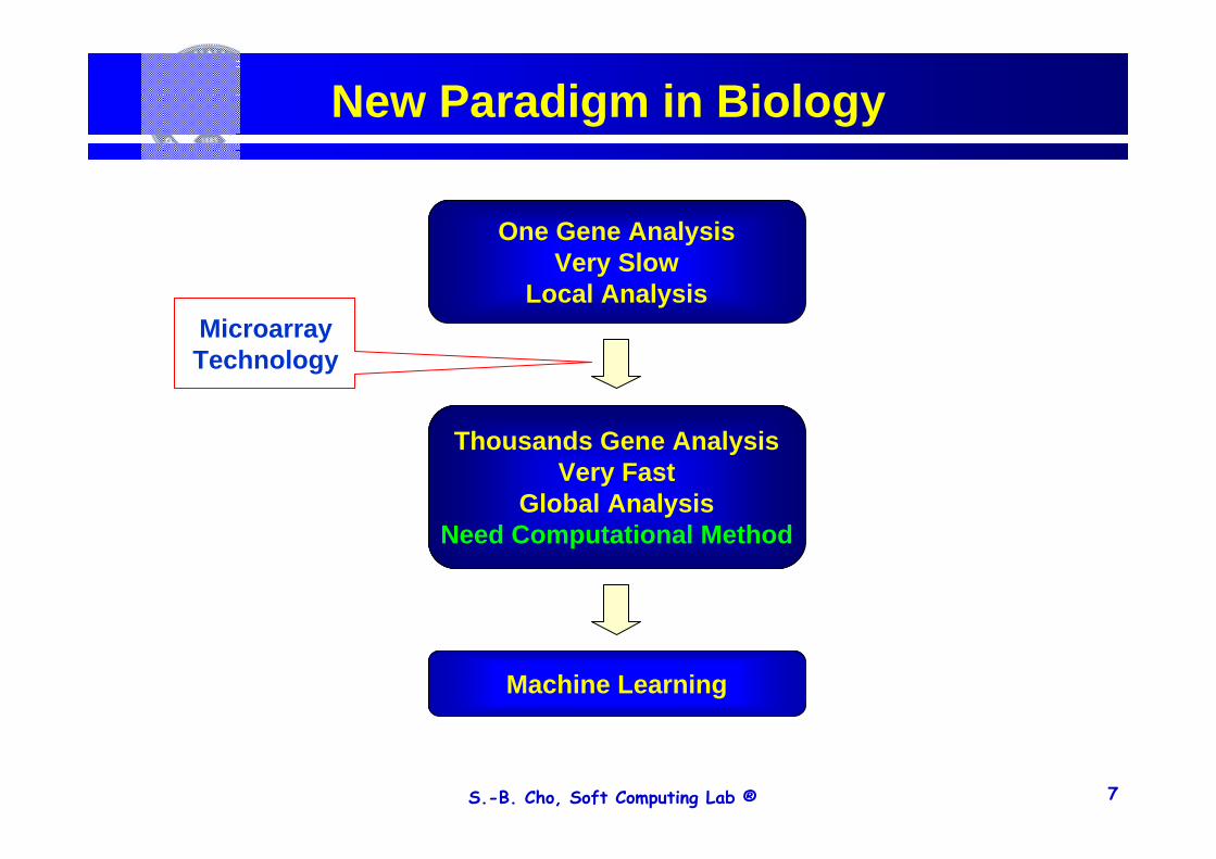
New Paradigm in Biology

Thousands Gene AnalysisVery Fast

Global AnalysisNeed Computational Method

MicroarrayTechnology

One Gene AnalysisVery Slow

Local Analysis

Machine Learning


Overview

DNA microarray– A chip or slide that has been printed with a large number of DNA

spots

DNA microarray technology– Enables the simultaneous analysis of thousands of gene

expression levels for genetic and genomic research and for diagnostics

– Gene : sequence of DNA that includes genetic information

Two major techniques– Hybridization method

cDNA microarray/ Oligonucleotide microarray– Sequencing method

Serial analysis of gene expression (SAGE)

DNA Microarray


Data Acquisition

microarray image

sample 1sample 2

sample 3

samples

gene

s

accumulated microarray image(colors)

gene expression data matrix(numbers)

)3()5(

2 CyIntCyIntlog

samples

gene

s

Microarray data consist of large number of genes in small samples!!

DNA Microarray


Example

Gene Description Gene Accession Number AML AML ALL AML AML ALL

GB DEF = BAC clone RG293F11 from 7q21-7q22, complete sequence AC000066_at 32 42 16 2 -26 39

Metabotropic glutamate receptor 8 mRNA AC000099_at 245 125 117 124 99 130

WUGSC:H_GS188P18.1a gene extracted from Human BAC clone GS188P18 AC000115_cds1_at -98 -19 97 86 -57 -78

A-589H1.1 from Homo sapiens Chromosome 16 BAC clone CIT987-SKA-589H1 ~complete genomic sequence, complete sequence./ntype=DNA /annot=mRNA

AC002045_xpt1_at 70 180 51 92 150 119

WUGSC:DJ515N1.2 gene extracted from Human PAC clone DJ515N1 from 22q11.2-q22 AC002073_cds1_at 146 224 634 15 -87 -1

GUANINE NUCLEOTIDE-BINDING PROTEIN G(T), ALPHA-1 SUBUNIT AC002077_at -260 -638 -322 -402 -862 -233

GB DEF = PAC clone DJ525N14 from Xq23, complete sequence AC002086_at 117 0 79 -12 -34 -5

COX6B gene (COXG) extracted from Human DNA from overlapping chromosome 19 cosmids R31396, F25451, and R31076 containing COX6B and UPKA, genomic sequence

AC002115_cds1_at 2236 5198 3001 4263 3083 3392

F25451_3 gene extracted from Human DNA from overlapping chromosome 19 cosmids R31396, F25451, and R31076 containing COX6B and UPKA, genomic sequence

AC002115_cds3_at 729 533 881 960 675 380

UPKA gene extracted from Human DNA from overlapping chromosome 19 cosmids R31396, F25451, and R31076 containing COX6B and UPKA, genomic sequence

AC002115_cds4_at -1031 -1029 -1266 -1667 -942 -223

A part of Leukemia dataset, before log transformation (Golub, et al., 1999)sample

gene

DNA Microarray


Two Types of Data

Single time point in different states – States : disease or tumor type– Goal : classifying samples using informative genes– Can be used for gene identification– Feature selection/extraction– Classification problem

Monitoring each gene in multiple times– Time series data– Goal : identifying functionally related genes– Can be used for gene regulatory network– Clustering problem

DNA Microarray


Challenges

Noise– Microarray data contain a high level of noise due to experimental

procedures– The labeling of cDNA and the scanning of the slides frequently

show non-linear characteristics

Sparseness– Microarray data are sparse– Several thousands of genes are monitored, while the number of

samples is often restricted to hundreds or less

High redundancy– Many genes are highly correlated, which leads to redundancy in

the data– Adding coexpressed genes to the classification system does not

increase information for the system

DNA Microarray


Classification

Comprehensive comparisonsEnsemble approaches


Motivation

Many researchers have been studying many problems of cancer classification using gene expression profiles and attempting to propose the optimal classification technique to work out these problems

We need a thorough effort to give the evaluation of the possible methods to solve the problems of analyzing gene expression data

There are several microarray datasets– leukemia cancer dataset, colon cancer dataset, lymphoma dataset,

breast cancer dataset, NCI60 dataset, and ovarian cancer dataset

Three datasets for our study– Leukemia cancer dataset– Colon cancer dataset– Lymphoma cancer dataset


Classification Scheme

Class 1

Class 2

Feature selection Classification

DNA microarray data Selected features


Overview

Selecting informative features appropriate to specific goalVariable selection/ gene selection

Microarray data consist of large number of genes in small samplesAll genes are not needed for classification

It is essential to select some genes highly related with particular classes for classification, which is called informative genes (Golub et al., 1999)

Many selection/extraction techniques based on measures– Correlation-based measures– Similarity-based measures– Information theory-based measures– Principal component analysis

Feature Selection


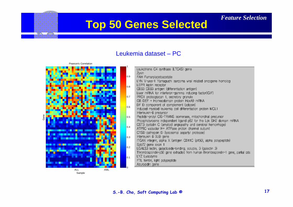
Top 50 Genes Selected

0

0.1

0.2

0.3

0.4

0.5

0.6

0.7

0.8

0.9

1

Sample

Gen

e

Pearson's Correlation

ALL AML

Leukemia dataset – PC

Feature Selection


Rank-based Selection

Representative feature selection methodGene selection according to the significance order of each gene

Gene number SignificanceGene 1 0.5Gene 2 0.7Gene 3 0.9Gene 4 0.6

Selecting order

Gene 3 Gene 2 Gene 4 Gene 1

Feature Selection

How can we calculate the significance?


Correlation Measures

Measuring how much each gene is correlated with the classgideal = (0, 0, 0, …, 1, 1, 1) class pattern

Pearson correlation coefficients (PC)– Parametric

Spearman correlation coefficients (SC)– Non-parametric

0 0.1 0.2 0.3 0.4 0.5 0.6 0.7 0.8 0.9 10

0.1

0.2

0.3

0.4

0.5

0.6

0.7

0.8

0.9

1

0 0.1 0.2 0.3 0.4 0.5 0.6 0.7 0.8 0.9 10

0.1

0.2

0.3

0.4

0.5

0.6

0.7

0.8

0.9

1

Positive correlation

Negative correlation

Feature 1

Feature 2

No correlationFeature 1

Feature 2

Feature Selection

class 1 class 2


Similarity Measures

Calculating geometrical similarity between ideal gene vector and each gene vector

Euclidean distance (ED)– Geometric distance

Cosine coefficient (CC)– Difference of direction

θ

d

Feature Selection


Information Theoretic Measures

Measuring feature-goodness based on the frequency of the feature satisfying condition Q (whether genes are induced or not)

Using frequency or mean and standard deviation of data to calculate the significance of genes

Information gain (IG)Mutual information (MI)Signal to noise ratio (SN)

1µ2µ

21 µµ −

1σ2σ

Feature Selection


Mathematical Definitions

)()()()(),(

)()(log

)()(log

)()(log

)(

)1()(61

))()()((

21

21

22cos

2

2

2

22

22

ggggcgP

CABAAMI

DBBABB

CABAAAIG

YXXYr

YXr

NNDyDxr

NYY

NXX

NYXXY

r

ine

euclidean

spearman

pearson

σσµµ

+−

=

+⋅+=

+⋅+⋅+

+⋅+⋅=

∑∑

∑=

−∑=

−−∑

−=

∑−∑

∑−∑

∑∑−∑=Pearson’s correlation

coefficient (PC)

Euclidean distance (ED)

Spearman’s correlationcoefficient (SC)

Cosine coefficient (CC)

Information gain (IG)

Mutual information (MI)

Signal to noise ratio (SN)

Feature Selection


Principal Component Analysis

Widely used for dimensionality reductionGiven N vectors in k-dimension, find c (<= k) orthogonal vectors that can be best used to represent data

The original data set is reduced to one consisting of N vectors on cprincipal components (reduced dimensions) Each vector is a linear combination of the c principal components

Principal components are directions of variance from the highest– The first principal component (PC) is the direction of maximum

variance, the second is that of the next highest variance, etc

∑=

=n

kkjikij mpt

1

n : the number of significant principal components pik : the score of sample i on component kmkj : the loading on component k of variable j

Feature Selection


Overview

Supervised learningNeed reliable and precise classification essential for successful cancer treatment Current methods for classifying human malignancies rely on a variety of morphological, clinical and molecular variablesUncertainties in diagnosis remain; likely that existing classes are heterogeneousCharacterize molecular variations among tumors by monitoring gene expression (microarray)

Hope: microarrays will lead to more reliable tumor classification (and therefore more appropriate treatments and better outcomes)

Decision boundary

Class 1

Class 2

Classifier


Classifiers

Multilayer perceptron

K-nearest neighbor

Support vector machine

Decision tree

Structure adaptive self-organizing map

Classifier


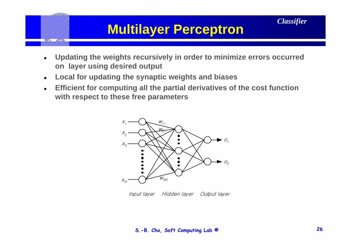
Multilayer Perceptron

Updating the weights recursively in order to minimize errors occurred on layer using desired outputLocal for updating the synaptic weights and biasesEfficient for computing all the partial derivatives of the cost function with respect to these free parameters

x1

x2

x3

xN

w11

w21

wKN

o1

o2

Input layer Hidden layer Output layer

Classifier


K-Nearest Neighbor

One of the most common methods in memory based induction

Deciding the labels of k known data based on similarities with known exemplars

– Sim(X, di) : Pearson’s correlation similarity function– k : # of neighbors – bj : a bias term

jjikNNd

ij bcdPdXcXPi

−= ∑∈

),(),Sim(),(

Classifier


Support Vector Machine

Introduced by Vapnik in 1995Constructing a hyperplane as the decision surface in such a way that the margin of separation between positive and negative examples is maximizedGiven a labeled set of M training samples (Xi, yi), where Xi ∈ RN and yiis the associated label, yi ∈ -1, 1, the discriminant hyperplane is defined by:

Linear and RBF kernels are used

∑=

+=M

iiii bXXkyXf

1),()( α

Classifier


Decision Tree

A graph (tree) based model used primarily for classificationPopular method for inductive inferenceA method for approximating discrete-valued target functionsEasy to convert learned tree into if-then rules

P2

P21

P32

P2 <= 0.03 P2 > 0.03

tumor

normal

P21 > 0.2P21 <= 0.2

normal tumor

P32 <= 0.22 P32 > 0.22

Classifier


Structure Adaptive SOM

Dynamic node splitting classifier based on self organizing map (SOM)Overcome the shortcoming of SOM– The structure of nodes does not have to be determined before

training in advance

P0 P4

P1

P2

P3

P0

P1

P2

P3

C0

C3C2

C1

Classifier


Classification Performance

MLP SASOMSVM KNN

Avg.Linear RBF Cosine PearsonPC 77.6 67.6 66.4 66.8 78.4 78.0 72.5SC 78.8 67.2 68.0 68.0 78.4 76.8 72.9ED 75.2 62.8 66.4 66.4 76.0 77.6 70.7CC 80.0 64.4 72.4 72.4 78.0 78.4 74.3IG 85.2 75.2 77.6 77.6 81.6 83.2 80.1MI 80.0 67.6 67.2 67.2 76.4 77.2 72.6SN 81.2 70.8 68.0 68.4 78.8 79.2 74.4

Avg. 79.7 67.9 69.4 69.5 78.2 78.6 73.9

Lymphoma cancer dataset

Comparisons


Classification Performance

MLP SASOMSVM KNN

DT Avg.Linear RBF Cosine Pearson

PC 74.2 74.2 64.5 64.5 71.0 77.4 41.9 66.8

SC 58.1 45.2 64.5 64.5 61.3 67.7 51.6 59.0

ED 67.8 67.6 64.5 64.5 83.9 83.9 54.8 69.6

CC 83.9 64.5 64.5 64.5 80.7 80.7 71.0 72.8

IG 71.0 71.0 71.0 71.0 74.2 80.7 67.7 72.4

MI 71.0 71.0 71.0 71.0 74.2 80.7 67.7 72.4

SN 64.5 45.2 64.5 64.5 64.5 71.0 54.8 61.3

Avg. 70.1 62.7 66.4 66.4 72.7 77.4 58.5 67.7

Colon cancer dataset

Comparisons


Classification

Comprehensive comparisonsEnsemble approaches


Overview

Limitation of machine learning classifiers in solving practical problems– Incomplete dataset– Noise in data– Imperfection of classification algorithm

Solution– Searching for effective features of input patterns

Utilizing multiple featuresProviding multiple pathways (more chance) to the optimal solution

– Improving classification performanceCombining multiple classifiersCombining several prospective models may produce better prediction

Ensemble Classifier


Rationale

High and complex space

1Φ

2Φ

3Φ F3

F2

F1

Optimal solution

Estimated solution by ensemble

Feature space Solution spaceSelected feature

Feature selection Classification

Ensemble Classifier


Ensemble Approach

A good ensemble includes base classifiers that– Are accurate

easy– Make their errors in different parts of the problem domain

difficult

Issues for ensemble classifiers– How to generate good base classifiers

From combinations of features and classifiers– How to combine the base classifiers

Majority votingWeighted votingBorda countBKS, …

Ensemble Classifier


Ensemble Generation

Feature selection

Pearson correlation coefficients (PC)Spearman correlation coefficients (SC)

Cosine coefficients (CC)Euclidean distance (ED)

Information gain (IG)Mutual information (MI)

Signal to noise ratio (SN)Principal component analysis (PCA)

Classification

Multilayer perceptron (MLP)K-nearest neighbor (KNN(C), KNN(P))

Support vector machine (SVM(L), SVM(R))Structure adaptive self-organizing map (SASOM)

Feature-classifier pair 1

Feature-classifier pair 2

Feature-classifier pair mn

… Huge number of available ensembles

2mn

m n

mn

Combination

Ensemble Classifier


Ensemble Strategies

Mutually exclusive features

Negatively correlated features

Combinatorial ensemble

GA optimization

Speciated GA optimization

Ensemble Classifier


Overview

Combining classifiers with mutually exclusive features through the analysis of correlation of features

Combiningmodule

Input pattern

SVMRBFSVMlinearKNNMLPSVMRBFKNNMLP SVMlinear

Featurea Featurebmutuallyexclusive

Mutually Exclusive Features


Classification Rates

40

50

60

70

80

90

100R

ecog

nitio

n ra

te [%

]

MLP KNN SVMRBF SVMlinear KNNcosine SOM DT

Leukemia dataset



Correlation of Features

Three representative cases of correlations– Pearson’s correlation between features has been calculated

Pearson’s correlation

(a) Negative correlation(coefficient: -0.52)

Euc

lidea

n di

stan

ce


(b) Neutral(coefficient: -0.03)

Sign

al to

noi

se r

atio


(c) Positive correlation(coefficient: 0.80)

Cos

ine

coef

ficie

nt



Comparison of Accuracy

case(a)Negative

correlation

case (b)Neutral

case (c)Positive

correlation

Rec

ogni

tion

accu

racy

[%]

all feature

41.2

64.7

85.391.294.197.1

100.0Neural networkMajority voting



Overview

Idea– With two ideal gene vectors, select features whose expression

patterns are similar to one of ideal gene vectors– Train classifiers with two feature sets and combine them

Method – Sim(X, Y) : similarity between vector X and Y

– Ideal gene vector AGene set whose expression pattern is similar to (1,1,1,…,0,0,0)SGS I = argmaxSim(genei, Ideal Gene Vector A)

– Ideal gene vector BGene set whose expression pattern is similar to (0,0,0,…,1,1,1)SGS II = argmaxSim(genei, Ideal Gene Vector B)

Negatively Correlated Features


Example

Ideal Gene A(1,1,1,1,1,1,0,0,0,0,0,0)

Ideal Gene B(0,0,0,0,0,0,1,1,1,1,1,1)

NegativeCorrelationGene 1 Gene 1'

Gene 2 Gene 2'



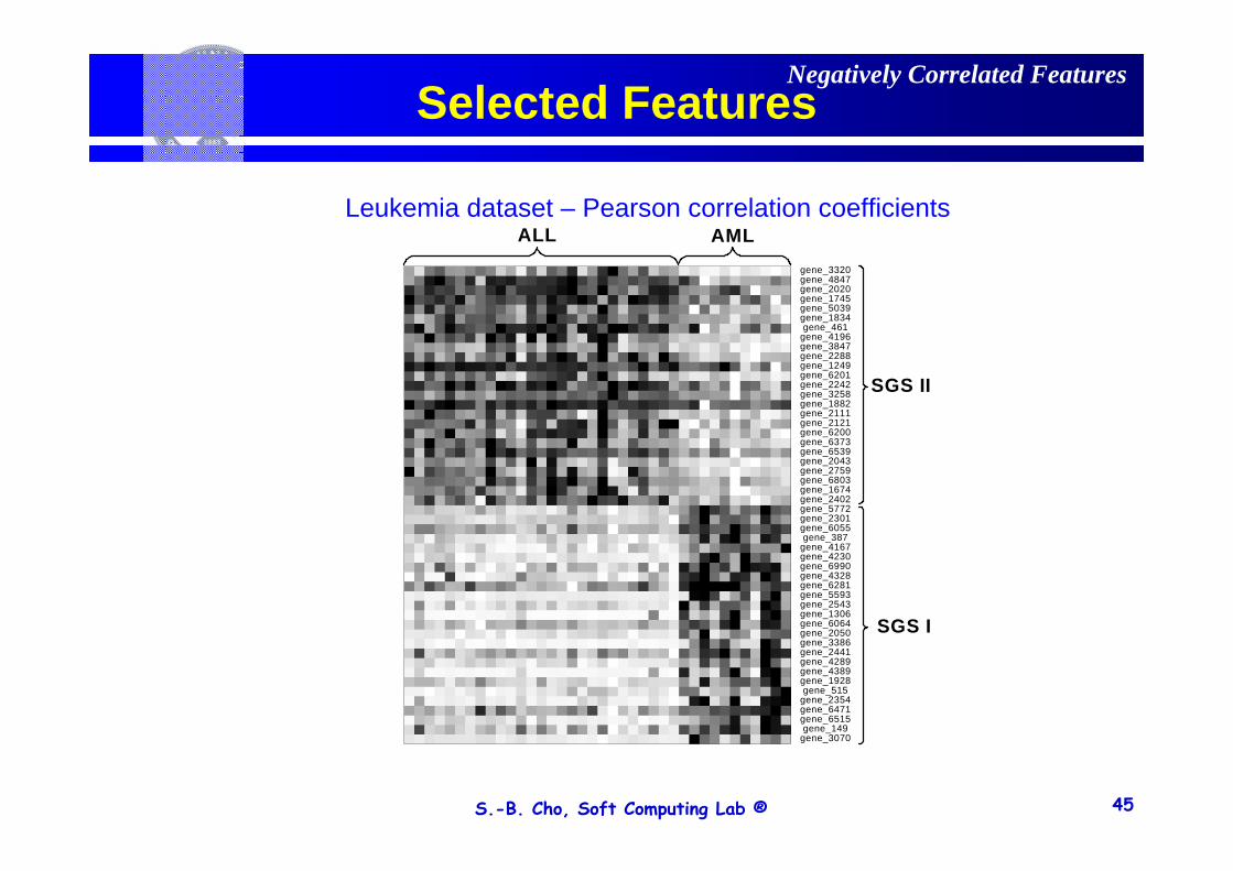
Selected Features

ALL AMLgene_3320gene_4847gene_2020gene_1745gene_5039gene_1834gene_461

gene_4196gene_3847gene_2288gene_1249gene_6201gene_2242gene_3258gene_1882gene_2111gene_2121gene_6200gene_6373gene_6539gene_2043gene_2759gene_6803gene_1674gene_2402gene_5772gene_2301gene_6055gene_387

gene_4167gene_4230gene_6990gene_4328gene_6281gene_5593gene_2543gene_1306gene_6064gene_2050gene_3386gene_2441gene_4289gene_4389gene_1928gene_515

gene_2354gene_6471gene_6515gene_149

gene_3070

SGS II

SGS I

Leukemia dataset – Pearson correlation coefficients



PCA 3D Plot

Select 25 genes from SGS I + 25 genes from SGS II by Pearson correlation coefficients and extract 3 principal components

Well classifying AML and ALL

-0.26-0.24

-0.22-0.2

-0.18-0.16

-0.14-0.12

-0.1-0.08

-0.4

-0.3

-0.2

-0.1

0

0.1

0.2

0.3

-0.4

-0.2

0

0.2

0.4

0.6

First PCSecond PC

Third

PC

Red : ALLBlue : AML



Comparison of Performance

accuracy(%) sensitivity(%) specificity(%)

Leukemia

MLP I 97.1 92.9 100.0

MLP II 82.4 64.3 95.0

MLP I + MLP II 97.1 92.9 100.0

Colon

MLP I 80.6 95.0 54.5

MLP II 77.4 95.0 45.5

MLP I + MLP II 87.1 95.0 72.7

Lymphoma

MLP I 64 36.4 85.7

MLP II 76 72.7 78.6

MLP I + MLP II 92 90.9 92.9



Overview

In theory, a good ensemble should include base classifiers that– Are accurate– Make their errors in different parts of the problem domain

In practice– Easy to obtain weak classifiers whose accuracy is about 50%– Very difficult to get uncorrelated classifiers

large number of classifiers do not guarantee the good performance of ensemble

Testing ensembles combinatorially until the promising number of ensembles instead of all available ensembles

Combinatorial Ensemble


Structure

GeneExpression

Data

F1

F2

F3

Fi

C1

C2

C3

Cj

...

...

Feature SelectionMethods

ClassifiersF1 C1

F1

C2

F1

C2

Fi Cj...

n Feature-Classifier Sets

Combinatorial

Selection

(nC5)

EnsembleMethod

1

c

...

Class prediction




Combining method # of classifiers Leukemia Colon Lymphoma

Majority voting

3 97.1 93.5 96.0

5 97.1 93.5 100.0

7 97.1 93.5 100.0

All 91.2 71.0 80.0

Weighted voting

3 97.1 93.5 96.0

5 97.1 93.5 100.0

7 97.1 93.5 100.0

All 97.1 71.0 88.0

Bayesian Combination

3 97.1 93.5 96.0

5 97.1 93.5 100.0

7 97.1 93.5 100.0

All 97.1 74.2 92.0

3 is less accurate, 7 is expensive



Overview

There are so many available ensembles from several classifiers– Exponentially increase with respect to the number of classifiers– 48 base feature-classifier pairs make

Exhaustive searching is very time-consuming

Use GA to find optimal ensemble in a short time – Ensemble is made from 48 base feature-classifier pairs from 8

feature selection methods and 6 classifiers

248 ensembles

GA Optimization


Structure

FeatureSelector

1

Classifier 1

Classifier 2

Classifier n

FeatureSelector

2

FeatureSelector

m

...

...

GA searching

... ...

x xo x o x

Cancer Normal

feature-classifier pairs

fitness evaluation

...

... ......

Normalized Gene Expression Profiles

Ensemble

GA Optimization


GA Chromosome

0

1

1

0

0

1

0

0

0

...

48 bits

CC-MLP

ED-MLP

IG-MLP

MI-MLP

PC-MLP

PCA-MLP

SN-MLP

SC-MLP

SC-SVM(RBF)

Genotype(chromosome)

Phenotype(feature-classifier)

...

1 0 1 0 1 0 1 1 - 62.5%

0 0 0 1 1 0 0 1 - 62.5%

1 1 0 0 0 1 0 1 - 75%

Result of feature-classifier pair

1 0 0 0 1 0 0 1 - 87.5%

1 1 0 0 1 0 0 1

ensemble result

actual class

Majority voting

Fitness of a chromosome ch:chchchFit

by samples classified totalof #by samples classifiedcorrectly of #)( =

GA Optimization


Change of Average Fitness

0 50 100 150 200 250 300 350 400 450 5000.81

0.82

0.83

0.84

0.85

0.86

0.87

0.88

0.89

0.9

0.91

Iteration

Fitn

ess

Increase until the number of iterations reaches 150Saturated after 150 iterations

GA Optimization


Leave-one-out-cross Validation

55

60

65

70

75

80

85

90

95

100

Acc

urac

y(%

)

Lymphoma Colon

training

training validation (single)

validation (single)

validation(ensemble) validation(ensemble)

test

test

range

average

Optimal ensemble searched by GA outperforms!!

GA Optimization



1 2 3 4 5 6 7 8 9 10

85

90

95

100

experiment

accu

racy

best singleensemble of good classifiersbest ensemble among 1 milion random ensemblebest ensemble among 1 milion - simple GA, sharingbest ensemble among 1 milion - crowding

GA > best single classifier > ensemble of good classifiers

GA Optimization


Some Optimal EnsemblesGA Optimization

Feature-classifier pair

Accuracy(%)

CC-KNN(P) 75.0

MI-KNN(C) 83.3

SN-KNN(C) 79.2

SC-SASOM 62.5

IG-SVM(L) 91.7

Ensemble 100

Feature-classifier pair

Accuracy(%)

IG-KNN(C) 91.7

MI-KNN(C) 83.3

SN-KNN(C) 79.2

SN-KNN(P) 79.2

CC-SASOM 54.2

IG-SASOM 83.3

PC-SVM(R) 62.5

Ensemble 100

Majority voting Weighted voting


Overview

Among all the 2mn ensembles– Standard GA does not guarantee optimal solution– GA usually converges to local optima

There may be many optimal ensembles– The number is unknown– GA just finds one of them

Use of speciated GA instead of standard GA

Fitness sharing Deterministic crowding

Speciated GA Optimization


Concept

Observation space

Solution space

genetic drift

Solutions searched by simple GASolutions searched by speciated GA

Ω



Structure

PC SC ED CC IG MI SN PCA

MLP KNN(C) KNN(P) SVM(L) SVM(R) SASOM

......

FC1 FC2 ...... FC48

......FC2

Ensemble maker

speciated GA searching

Optimal ensemble

Tumor Normal

new instance

Feature selection

Classifier

FCs

Ensemble

Searching

Evaluation

Training

Validation

Test

Microarray data

Gene expression data matrixPreprocessing



Fitness Function

)(1*)()( chNumchAccchFitness α−=

Fitness of a chromosome ch

chchchAcc

by samples classified totalof #by samples classifiedcorrectly of #)( =

chchNum chromosomein s1'bit of #)(1 =

constant:α

where The shorter, the better



Deterministic Crowding

Input: g - number of generations to run, s - population sizeOutput: P(g) - the final population

P(0) initialize()for t 1 to g do

P(t) shuffle(P(t-1))for i 0 to s/2 -1 do

p1 a2i+1(t)p2 a2i+2(t)c1, c2 recombination(p1, p2)c1' mutate(c1)c2' mutate(c2)if[d(p1,c1')+d(p2,c2')] ≤ [d(p1,c2')+d(p2,c1')] then

if F(c1') > F(p1) then a2i+1(t) c1' fiif F(c2') > F(p2) then a2i+2(t) c2' fi

elseif F(c2') > F(p1) then a2i+1(t) c2' fiif F(c1') > F(p2) then a2i+1(t) c1' fi

fiod

Od



Fitness Sharing

A strategy that maintains diversity of chromosomes through lowering the fitnesses of individuals that are located close– Use shared fitness F’(i) instead of original fitness F(i)

)()()('imiFiF =

∑−

=µ

1)),(()(

jjidshim =)(dsh

otherwise 0 if )/(1 shareshare σdd <− ασ

sharing

fitness

shared fitness



Comparison of Diversity

Experiment sGA sharing crowding1 1 1 2462 0 0 533 0 0 1134 1 1 3455 2 1 4606 0 0 207 0 0 678 0 0 1979 1 1 37810 1 2 233

The number of optimal ensembles found by each method on one dataset

crowding >> sGA ≈ sharing



Change of Fitness and Accuracy

0 100 200 300 400 500 600 700 800 900 10000.6

0.65

0.7

0.75

0.8

0.85

0.9

0.95

1

iteration

fitne

ss, a

ccur

acy

simple GA, fitnesssimple GA, accuracysharing, fitnesssharing, accuracycrowding, fitnesscrowding, accuracy

crowding >> sGA ≈ sharing



Search Efficiency

Common GA Sharing Crowding

0

200

400

600

800

1000

1200

Itera

tions

Execution time per iteration: simple GA < crowding < sharing



Conclusion

Classification – Comparisons of feature/classifiers– Exploration of ensemble approaches

hybrid intelligent systems for dna microarray data...

Documents