hybrid combining of directional antennas for periodic
TRANSCRIPT

Hybrid Combining of Directional Antennas for Periodic BroadcastV2V Communication
Downloaded from: https://research.chalmers.se, 2021-11-24 05:26 UTC
Citation for the original published paper (version of record):Bencheikh Lehocine, C., Ström, E., Brännström, F. (2020)Hybrid Combining of Directional Antennas for Periodic Broadcast V2V CommunicationIEEE Transactions on Intelligent Transportation Systems, In Presshttp://dx.doi.org/10.1109/TITS.2020.3033094
N.B. When citing this work, cite the original published paper.
©2020 IEEE. Personal use of this material is permitted.However, permission to reprint/republish this material for advertising or promotional purposesor for creating new collective works for resale or redistribution to servers or lists, or toreuse any copyrighted component of this work in other works must be obtained fromthe IEEE.
This document was downloaded from http://research.chalmers.se, where it is available in accordance with the IEEE PSPBOperations Manual, amended 19 Nov. 2010, Sec, 8.1.9. (http://www.ieee.org/documents/opsmanual.pdf).
(article starts on next page)
1
Hybrid Combining of Directional Antennas forPeriodic Broadcast V2V Communication
Chouaib Bencheikh Lehocine, Erik G. Strom, Senior Member, IEEE, and Fredrik Brannstrom, Member, IEEE
Abstract—A hybrid analog-digital combiner for broadcastvehicular communication is proposed. It has an analog part thatdoes not require any channel state information or feedback fromthe receiver, and a digital part that uses maximal ratio combining(MRC). We focus on designing the analog part of the combinerto optimize the received signal strength along all azimuth anglesfor robust periodic vehicle-to-vehicle (V2V) communication, in ascenario of one dominant component between the communicatingvehicles (e.g., highway scenario). We show that the parametersof a previously suggested fully analog combiner solves theoptimization problem of the analog part of the proposed hybridcombiner. Assuming L directional antennas with uniform angularseparation together with the special case of a two-port receiver,we show that it is optimal to combine groups of dL/2e andbL/2c antennas in analog domain and feed the output of eachgroup to one digital port. This is shown to be optimal undera sufficient condition on the sidelobes level of the directionalantenna. Moreover, we derive a performance bound for thehybrid combiner to guide the choice of antennas needed to meetthe reliability requirements of the V2V communication links.
Index Terms—Broadcast V2V communication, directional an-tennas, hybrid combining, periodic communication.
I. INTRODUCTION
COOPERATIVE intelligent transportation systems (C-ITS) have the promise to make our roads safer, more
efficient, and environment-friendly. To enable cooperationbetween intelligent transportation systems, vehicular commu-nication is needed. In contrast to applications supported by tra-ditional mobile broadband communication, C-ITS applicationscan have ultra high requirements on reliability and latency,and good designs of antenna systems are key to meet thosereliability requirements. Typically, vehicles are equipped withomnidirectional antenna elements that are mounted on theroof. However, the vehicle body and the mounting positionof antennas affect the omnidirectional characteristics of theradiation patterns [1], [2]. Consequently, the distorted omni-directional pattern may have very low gains or blind spots atcertain azimuth angles. In scenarios where the received signalhas only one dominant component, e.g., highway scenarios,problems of decoding the packets may arise if the angle ofarrival (AOA) of the signal coincides with a very low gain ofthe receiving antenna. Hence, we need the antenna system tobe robust in all directions of arrivals.
This research has been carried out in the antenna systems center ChaseOnin a project financed by Swedish Governmental Agency of Innovation Systems(Vinnova), Chalmers, Bluetest, Ericsson, Keysight, RISE, Smarteq, and VolvoCars.
The authors are with the Communication Systems Group, Departmentof Electrical Engineering, Chalmers University of Technology, 412 96Gothenburg, Sweden (e-mail: [email protected]; [email protected];[email protected])
For a robust broadcast antenna system in spite of bodyand placement effects, multiple antennas with complementarypatterns can be combined to achieve an effective patternwith better omnidirectional characteristics than the distortedpatterns of single antennas. In particular, directional antennasthat are pointing towards different directions can be used forthis purpose. Since the main contribution of these antennasis through the main lobe, we may have more flexibility—compared to omnidirectional antennas—in mounting themsuch that the distortions do not coincide with their main lobes.That may reduce the severity of distortions and lead to anoverall better effective pattern.
The classical way of combining antennas is done in thedigital domain through either selection combining (SC), equalgain combining (EGC), or maximal ratio combining (MRC). Ingeneral, these fully digital solutions require a radio frequency(RF) chain per antenna element which results in high cost andpower consumption.
A recent trend in deploying multiple antenna systems is theuse of hybrid analog-digital combiners/beamformers. Hybridcombiners (HCs) require less number of RF chains thanantennas, which translates to a reduction of cost and powerconsumption with respect to the fully digital solutions. HCshave been studied extensively and state-of-the-art designs andparadigms are well summarized in [3]–[5]. The main archi-tectures considered use phase shifters in the RF part, whichlimits the HC to have a constant-modulus complex RF weight.Design strategies of HCs take into account instantaneous oraverage channel state information (CSI) to attempt findingthe optimal analog and digital combining coefficients [4]. Thedesign objective is, typically, maximizing the rate or the signal-to-noise ratio (SNR) experienced by the user [3]. An exampleof a study of HCs that take into account vehicular usersis [6]. There, a general framework is set for the design ofhybrid beamformers/combiners according to three main archi-tectures. Performance is evaluated in a cellular infrastructure-to-everything scenario considering vehicular users.
Aside from the fully digital and hybrid combining schemes,fully analog solutions have been investigated in several pub-lications including [7] and [8]. In [7], three architectures ofanalog combiners (ACs) have been proposed. The differentarchitectures have varying complexity depending on the com-bination of RF components used (variable gain amplifiers,variable gain amplifiers and sign switches or variable phaseshifters). Optimization of the RF weights in these architectureswas done with the objective of maximizing the SNR at theoutput of the combiner, assuming perfect knowledge of CSI.In [8], an analog combiner based on phase shifters was pro-posed for broadcast vehicle-to-vehicle (V2V) communication.
V2V broadcast communication is mainly based on periodicdissemination of status messages. The solution presented in [8]takes advantage of the periodic behavior of the status messagesand the redundancy of their content and attempt to findthe optimal phase shifters that minimize the probability ofconsecutive packet errors in the system. That is done inabsence of CSI or feedback from the receiver. Hence, besidethe low cost and low power consumption, this AC has verylow complexity. However, it does not leverage on the benefitof digital combining.
To take advantage of digital combining high performancebenefits and analog combining low-cost, low-complexity bene-fits, we propose, in this work, a hybrid analog-digital combinerthat is tailored for periodic broadcast V2V communication. Wetake a modular approach in our HC design, that is, we assumethat the digital baseband combining is done using a multiportreceiver that applies standard MRC. Given that we do not haveaccess to CSI or any feedback from the receiver, we attemptto design the analog part of the HC to minimize the errorprobability of consecutive status messages. That is a similardesign approach to what was followed in [8]. The proposedHC has the advantage of having the analog part independentof the digital part. Hence, the RF part can be located closer towhere the antennas are placed. Moreover, we use directionalantennas in this setting and we investigate the optimal HCconfiguration, i.e., the optimal way to connect antennas to thedigital ports, in the special case of a two-port digital receiver.The main contributions of this work can be summarized asfollows.• We propose a hybrid low-cost combining scheme for
broadcast vehicular communication that results in robustperformance at all AOAs.
• We show that the obtained parameters for the phase shiftnetwork in [8] are also a solution to the optimizationof the analog part of HC when MRC is used in base-band. Depending on the setup, the proposed HC eitherminimizes or provides a lower bound on the burst errorprobability of the full system.
• We analytically identify the optimal number of antennasper port when feeding L directional antennas to the HCwith two digital ports. It is found that it is optimal to feeddL/2e antenna to one port and bL/2c antenna to the otherport, when a sufficient condition on the sidelobes of theantennas is satisfied.
• In addition, we derive a performance bound of the HC,which can be used as a guideline when designing theantenna system.
II. SYSTEM MODEL
In this section we start by presenting the system model. Wenote that this is the system model as presented in [8], extendedto multiple ports receiver case.
A. Antenna System
We assume the use of L antennas that are mounted atthe same height on the vehicle. The antennas are verticallypolarized [9]. Taking into account the relative comparable
height of different vehicles, we assume that the incident wavesarrive in the azimuth plane. Thus, we can represent the far-field response of the antennas as a function of the azimuthangle φ only. That is,
gl(φ, θ) = gl(φ, π/2) = gl(φ), (1)
where θ is the elevation angle and l is the antenna index.
B. Channel Model
We consider a scenario of vehicle-to-vehicle communicationin a scarce multi-path (MP) environment with a dominantcomponent. This component could be a line-of-sight (LOS)or a first order single bounce reflection from a local reflector.This is typical in communication between cars in highways.In such scenario, it has been shown through measurementsthat only a few MP components with small azimuth angularspread contribute to the total received power [10]. Thus, thechannel gain at an antenna output can be modeled by a singledominant component arriving at a particular AOA φ. Takinginto account the far-field function of the receiver antennas, thechannel gain of antenna l can be stated as [11, Eq. 8]
hl(t) = a(t)gl(φ)e−Ωl(t), (2)
where a(t) and Ωl(t) are the complex gain and the phase shift,respectively, of the dominant MP component with AOA φ,received at antenna l. The phase shift depends on the distanceas Ωl(t) = 2π
λ dl(t), where λ is the wavelength of the carrierfrequency and dl(t) is the distance of the path followed fromthe transmitter to the lth receiver antenna. Taking the antennawith index l = 0 as a reference, we can express the relativephase differences with respect to the reference antenna asΩl(t) = Ωl(t) − Ω0(t) with Ω0(t) = 0. The channel modelcan be expressed consequently as
hl(t) = a(t)gl(φ)e−Ωl(t), (3)
with a(t) = a(t)e−Ω0(t). The relative phase differences canbe assumed slowly varying over a period of a few seconds.This holds if the main component between the two vehicleswith approximately the same AOA is still present over thatduration. From (3) we can see that in case an antenna l haspoor gain at the AOA of the signal, the received power will below, which could lead to the loss of the received packet. Thus,we aim to design our analog combiner such that the overallscheme is robust for any AOA.
C. IEEE802.11p Broadcast Communication
Cooperative awareness in intelligent transportation systemsthat are based on IEEE802.11p, is created through the dissem-ination of periodic messages that contain status informationlike position, speed, heading, lane position, etc. These arecalled cooperative awareness messages (CAMs). CAMs aretransmitted periodically with a frequency that is dependenton both the change of status of the transmitting vehicle (e.g.,change of lane), and on the traffic on the radio channel [12].The period between two consecutive CAMs, T , has a mini-mum duration of 100 ms and a maximum of 1000 ms [12],
Page 2
while the duration of a CAM packet Tm is in the range of0.5−2 ms [8]. We note that the period is much longer than thepacket duration, T Tm. Due to the high frequency of CAMdissemination, their content is highly correlated over the timeof few periods. At the level of a C-ITS application runningon a vehicle, if a CAM packet from a neighboring vehicleis lost, the C-ITS application can still use the previouslyavailable status information about the neighboring vehicle andfunction properly. This is provided that the age of the alreadyavailable status information is not too large (i.e., the availablestatus information is not outdated). Following this line ofthought, it has been proposed in several works including [13],to assess the reliability of broadcast V2V systems using age-of-information rather than the classical overall packet deliveryratio metric. The age-of-information at a certain time instanceis equal to the latency of the latest successfully received packetplus the time elapsed since its reception. We recall that latencyof a packet is commonly defined as the time elapsed betweenthe generation and reception of the packet. If we considerthe latency as negligible or fixed from packet to packet, therandomness in the age-of-information peak values is deter-mined by the time separating two consecutive successful CAMpacket receptions. We note that packet inter-reception time(acronymed IRT or PIR) and T-window are similar metricsand they are elaborated in [14], [15], and [16], respectively.To relate the application-level age-of-information metric tothe reliability of V2V communication, a parameter labeledBurst Error probability (BrEP) has been proposed and usedin [8] to design an analog combiner for V2V communication.Using this parameter, outage is declared when K consecutiveCAMs are not decoded correctly. In our work we follow asimilar approach, that is, taking into account the correlatedstatus information (position, speed, heading, lane position,etc.) contained in consecutive CAMs, we assume that onlysome packets out of a burst of K consecutive CAMs need tobe decoded correctly for the proper functionality of a particularC-ITS application that depend on their content. Therefore, wetarget the minimization of the BrEP of K CAMs, which iflatency is negligible (or constant) is equivalent to minimizingthe probability of not satisfying the maximum allowable age-of-information Amax = KT (or Amax = KT + const.) setby the C-ITS application. Aside from reliability, robustness isan important quality of V2V broadcast systems. To take thatinto account in our design, we consider a scenario where theAOA remains approximately constant for the time it takes totransmit K packets. In such case, there is a risk of losingall the K packets if the AOA coincides with a blind spot ora notch of low gain of the radiation pattern of the receivingantenna system. Hence, we target to combine the antennas tominimize the probability that a burst of K consecutive packetsis received with error when the AOA coincides with the worst-case AOA.
D. Analog Combiner
Given L antennas, we use an AC to combine these antennasignals to P < L receiver ports. The digital receiver performsMRC based on the estimated effective channel and noise
variance after the analog combining. The AC does not useany CSI or feedback from the receiver. Therefore, we restrictit to be composed of time varying phase shifters and adders.The phase shifters are modeled as a linear function of time.The complex analog gain from antenna l to port p is modeledas
sl,pe(αl,pt+βl,p) (4)
where αl,p and βl,p are the slope and the initial phase offset,respectively, of the time-varying analog phase shifter, andsl,p ∈ R is the gain from the output of antenna l to the inputof port p. For the AC to be power-conserving, it must satisfy
P−1∑p=0
s2l,p = 1. (5)
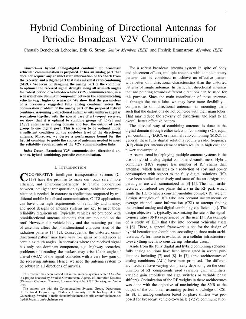
We define S ∈ RL×P to be the matrix with elements [S]l,p =sl,p. Depending on how antennas are connected to RF chains,the HC can have either a sub-connected, a fully-connected oran overlapping configuration [3]. As shown Fig. 1(a), in thesub-connected configuration each antenna is connected to onlyone RF chain. This results in P disjoint groups, each groupcomprised of Lp > 0 antennas and
∑P−1p=0 Lp = L. The set of
sub-connected configurations can be expressed as
S =S ∈ 0, 1L×P :
STS = diag(L0, L1, . . . , LP−1),
P−1∑p=0
Lp = L. (6)
In the fully connected configuration all antennas are connectedto all RF chains as shown in Fig. 1(b), while in the overlappingconfiguration at least one antenna is connected to more thanone RF chain. Although the fully connected and overalppingconfigurations are more general than the sub-connected con-figuration, they have the drawback that the noise componentsat the receiver ports might be correlated, which complicatesthe optimal digital receiver. Moreover, the fully connected andoverlapping configurations imply the use of power splitters,which leads to insertion loss and added complexity. For thesereasons, we chose in this paper to design the HC following asub-connected configuration.
III. DESIGN OF THE ANALOG COMBINER
A. SNR after the Hybrid Combining
We start by deriving the SNR expression of a receivedpacket after the analog combining and MRC, where the analogcombining is performed in sub-connected fashion with lineartime varying phase shifters. We have that the received signalat the output of antenna l is given by
yl(t) = hl(t)x(t) + nl(t), (7)
where x(t) is the transmitted signal, hl(t) is the channel gainat the antenna input modeled by (3) and nl(t) is independent,zero-mean complex Gaussian and white noise over the signal
Page 3
RF chain
RF chain
Digital
Combining
(MRC)
DataP
L0
LP−1
(a) Sub-connected configuration
RF chain
RF chain
Digital
Combining
(MRC)
DataPL
(b) Fully-connected configuration
Fig. 1. Sub-connected and fully connected architectures of Hybrid combiners.
bandwidth, with average power σ2n. Given the analog combiner
complex gain modelled by (4), the input to receiver port p is
rp(t) =
L−1∑l=0
sl,pe(αl,pt+βl,p)yl(t)
= a(t)x(t)
L−1∑l=0
sl,pgl(φ)e−(
Ωl(t)−αl,pt−βl,p)
+
L−1∑l=0
sl,pnl(t)e(αl,pt+βl,p)
= a(t)x(t)cp(t) + np(t), (8)
where cp(t) and np(t) are the equivalent channel gains andnoise signals respectively, at the input of receiver port p.Since np(t) is a sum of phase shifted zero-mean complexGaussian white noise signals, it has a Gaussian distributionCN (0, Lpσ
2n), where Lp =
∑L−1l=0 sl,p is the number of
antennas connected to port p.We assume that the time variation of the equivalent gain
cp(t) is negligible over the duration of a packet Tm, andtherefore we make the approximation
cp(t) ≈ cp(kT ), kT ≤ t ≤ kT + Tm, k = 0, . . . ,K − 1.(9)
Moreover, as stated before, in our scenario of interest therelative phase difference Ωl(t) can be assumed to experiencenegligible variation over a duration KT [8] and thus, it can beapproximated as Ωl(t) ≈ Ωl , Ωl(0). Furthermore, we defineψl,p , mod (Ωl − βl,p − ∠(gl(φ)), 2π) to accommodatefor the effective phase response at antenna l and we writecp adopting the previous approximations as,
cp(kT ) =
L−1∑l=0
sl,p|gl(φ)|e−(ψl,p−αl,pkT ). (10)
The receiver uses a MRC weight vector to combine the signals.In the sub-connected configuration there is no correlationbetween the noise processes at the input of the receiver,and therefore the optimal MRC weight applied at port p isc∗p(kT )/Lp [17]. Following that, the SNR of the kth packetafter the MRC can be found to be
γk =Pr
σ2n
P−1∑p=0
|cp(kT )|2
Lp, (11)
where Pr = E|a(t)x(t)|2 is the average signal power,and it is assumed to remain constant over the period of Kconsecutive packets.
We would like to express γk as a function of the ACparameters that need to be optimized. We note that only phaseslopes αl,p of the phase shifters that are connected to a port,i.e., for the pairs (l, p) such that sl,p = 1, need to be consideredin the optimization problem. Therefore, we define the vectorsαp ∈ RLp , p = 0, 1, . . . , P − 1 where
[αp]i : i = 0, . . . , Lp − 1 = αl,p : sl,p = 1,
l = 0, ..., L− 1. (12)
We assume that the mapping between the elements of the setsis such that it assigns i = 0 in the first set to the smallest l inthe second set, and i = 1 to the second smallest l and so on.We also define the vectors ψp as [ψp]i, i = 0, ..., Lp − 1 =ψl,p : sl,p = 1, l = 0, ..., L − 1, where the mapping from ito l is similar to the mapping used when defining the vectorsαp. Moreover, we define L-element vectors, α and ψ as α =[αT
0,αT1, ...,α
TP−1]T and ψ = [ψT
0,ψT1, ...,ψ
TP−1]T. Then, we
can readily express the SNR in (11) as γk(φ,S,ψ,α).
B. Optimization Problem of the Analog CombinerTo formulate the optimization problem of the analog part
of the HC, the burst error probability needs to be derived.Given a burst of K packets, under the assumptions thatpackets are of the same length, are transmitted using thesame modulation and coding scheme, and packet errors arestatistically independent, the BrEP is
PB(φ,S,ψ,α) =
K−1∏k=0
Pe
(γk(φ,S,ψ,α)
), (13)
where Pe(γk(φ,S,ψ,α)) is the packet error probability (PEP)of the kth packet. Since we are interested in robustness,the design goal is to minimize the bust-error probability forthe worst-case propagation, i.e., when all power arrives inthe least favorable AOA, and the worst-case effective phaseresponse at the antennas outputs, ψ. Design variables arethe grouping configuration and phase slopes defined by Sand α, respectively. Hence, the optimal analog combiner isdetermined by S? and α?, where
(S?,α?) , arg infS∈Sα∈RL
supφ∈[0,2π)
ψ∈[0,2π)L
PB(φ,S,ψ,α). (14)
Page 4
We will start by finding the optimal phase slopes for a givenconfiguration S, i.e.,
α?(S) = arg infα∈RL
supφ∈[0,2π)
ψ∈[0,2π)L
PB(φ,S,ψ,α), (15)
and then find the optimal configuration as
S? = arg infS∈S
supφ∈[0,2π)
ψ∈[0,2π)L
PB(φ,S,ψ,α?(S)). (16)
C. Optimal Phase Slopes
The choice of the phase slopes αl,p applied to the antennas,is made according to (15). The solutions to this optimizationproblem depends on the PEP function. For the special case ofexponential PEP function defined as
Pe(γ) = a exp(−bγ), (17)
where a, b > 0 are constants, the BrEP can be expressed as
PB(φ,S,ψ,α) = aK exp(− b
K−1∑k=0
γk(φ,S,ψ,α)). (18)
To solve (15), we first formulate a problem to find the optimalphase slopes for any AOA, that is α?(φ,S). Then, we candeduce the optimal phase slopes for the worst-case AOA. Wehave,
α?(φ,S) = arg infα∈RL
supψ∈[0,2π)L
PB(φ,S,ψ,α). (19)
Introducing the logarithm function to (18) and substituting inthe previous equation, we get
α?(φ,S) = arg infα∈RL
supψ∈[0,2π)L
ln(PB(φ,S,ψ,α)
)= arg sup
α∈RLinf
ψ∈[0,2π)L
K−1∑k=0
γ(φ,S,ψ,α, k)
= arg supα∈RL
infψ∈[0,2π)L
=J(φ,S,ψ,α)︷ ︸︸ ︷P−1∑p=0
K−1∑k=0
|cp(kT )|2
Lp︸ ︷︷ ︸=Jp(φ,S,ψp,αp)
. (20)
We note that the elements αp that compose the vec-tor α are independent of each other. The same thing ap-plies to ψ. Following that, we can decompose the jointoptimization of J(φ,S,ψ,α) to the separate optimizationof the terms Jp(φ,S,ψp,αp). After separate optimizationof these terms, we can readily reconstruct the optimalphase slopes vector for the overall system as α?(φ,S) =[α?0(φ,S),α?1(φ,S), ...,α?P−1(φ,S)]T where
α?p(φ,S) = arg supαp∈RLp
infψp∈[0,2π)Lp
Jp(φ,S,ψp,αp). (21)
The problem in (21), i.e., the optimization of an analogcombiner for a single port receiver, has been tackled in [8]. Thesolutions to this problem are stated in the following theorem.
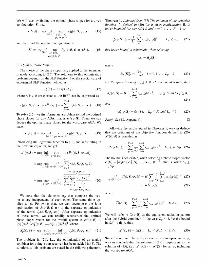
Theorem 1. [adopted from [8]] The optimum of the objectivefunction Jp defined in (20) for a given configuration S, islower bounded for any AOA φ and p = 0, 1, . . . , P − 1 as,
J?p (φ,S) ≥ K 1
Lp
L−1∑l=0
sl,p|gl(φ)|2, Lp ≤ K, (22)
this lower bound is achievable when selecting
αp = αp(S),
where
[αp(S)]i =i2π
KT, i = 0, 1, . . . , Lp − 1. (23)
For the special case of Lp ≤ 3, this lower bound is tight, thus
J?p (φ,S) = K1
Lp
L−1∑l=0
sl,p|gl(φ)|2, Lp ≤ K and Lp ≤ 3,
(24)and
α?p(φ,S) = αp(S), Lp ≤ K and Lp ≤ 3. (25)
Proof. See [8, Appendix].
Following the results stated in Theorem 1, we can deducethat the optimum of the objective function defined in (20)J?(φ,S) is bounded as
J?(φ,S) ≥ KP−1∑p=0
1
Lp
L−1∑l=0
sl,p|gl(φ)|2, Lp ≤ K,∀p. (26)
The bound is achievable, when selecting a phase slopes vectorα(S) = [αT
0(S), αT1(S), . . . , αT
P−1(S)]T. That is, when Lp ≤K, ∀p,
infψ∈[0,2π)L
J(φ,S,ψ, α) = K
P−1∑p=0
1
Lp
L−1∑l=0
sl,p|gl(φ)|2 (27)
= KG(φ,S), (28)
where
G(φ,S) =
P−1∑p=0
1
Lp
L−1∑l=0
sl,p|gl(φ)|2, S ∈ S. (29)
We will refer to G(φ,S) as the equivalent radiation patternafter the hybrid combiner. In the case Lp ≤ 3, ∀p the boundin (26) is tight, thus
α?(φ,S) = α(S), Lp ≤ K,Lp ≤ 3,∀p. (30)
Since the optimal phase slopes vectors are independent of φ,we can conclude that the solution of (19) is equivalent to thesolution of (15), i.e., α?(φ,S) = α?(S) for all φ, includingthe worst-case AOA.
Page 5
D. Optimal Sub-connected Configuration
In (16) we stated the problem of finding the optimal sub-connected configuration S? that corresponds to the optimalphase slopes α?(S), defined according to (15). In the pastsubsection we found the phase slopes α(S) that ensures anupper bound on the BrEP for the configurations S ∈ S :Lp ≤ K,∀p. For the configurations in the subset S ∈ S :Lp ≤ K and Lp ≤ 3,∀p, the phase slopes are optimal, thatis, α(S) = α?(S). However, for the configurations S ∈ S :∃p, Lp > K, no analytical solution is available for phaseslopes that minimizes or achieves an upper bound on BrEP.Taking that into account, let us define a subset of S,
S = S ∈ S : Lp ≤ K, ∀p (31)
together with an optimization problem to find the optimalconfiguration for the hybrid combiner with an analog part thatuses phase shifters with slopes α(S), that is
S , arg infS∈S
supφ∈[0,2π)
ψ∈[0,2π)L
PB(φ,S,ψ, α(S)). (32)
The solution to (16) for the configurations S ∈ S : Lp ≤ Kand Lp ≤ 3,∀p is a special case of (32). We follow similarsteps as used to derive (20) to express (32) as
S = arg supS∈S
infφ∈[0,2π)
ψ∈[0,2π)L
J(φ,S,ψ, α) (33)
= arg supS∈S
infφ∈[0,2π)
KG(φ,S), (34)
where (34) follows from (27). The optimal configuration Sdepends on the radiation patterns of the combined antennas.Given a set of antennas, we pick the configuration thatsatisfies (34). That is the configuration that maximizes thesum of the SNRs from the K packets for the worst-case AOAφ. Since the BrEP is inversely proportional to the equivalentgain G(φ,S) for all φ, the overall system performance canbe assessed according to the gain of the worst-case AOAof the equivalent radiation pattern after hybrid combining,minφG(φ,S). We observe that S maximizes the bound onJ?(φ,S) in (26). Hence, the hybrid combiner with the con-figuration S gives the best upper bound on the BrEP at theworst-case AOA. We identify two special cases of (32),
• If S = S = S ∈ S : Lp ≤ K and Lp ≤ 3,∀p,then the solution to (14) is given by (S?,α?) = (S, α).That is the optimal sub-connected analog combiner thatminimizes the BrEP for the worst AOA when MRC isused for digital combining.
• If S = ∅ then we need to solve (14) numericallyto attempt to find phase slopes and configuration thatminimizes or achieves an upper bound on the BrEP.
Assuming that S 6= ∅, we expect high performance, i.e., a highgain at the worst-case AOA of the equivalent radiation patternafter the HC with an analog part defined by (S, α(S)) andMRC combining. To assess the limits of the hybrid combiner,a performance bound is derived in the following lemma.
Lemma 1. Let G(φ,S) be defined according to (29) and letthe average radiation of all antenna elements be the same inthe azimuth plane, that is
1
2π
∫2π
|gl(φ)|2dφ = G2π, ∀l. (35)
Then,inf
φ∈[0,2π)G(φ, S) ≤ PG2π, (36)
where S is defined according to (32).
Proof. See Appendix A.
An example of a scenario where (35) holds is the deploy-ment of identical directional antennas pointing at differentdirections along the azimuth plane. We can observe from theright-hand side of (36) that the bound on the performance isproportional both to the average gain of the antenna elementsand the number of ports. However, it is not dependent on thenumber of antennas L. In Section V, it will be shown throughsome examples, that the performance bound can be approachedwith limited number of directional antennas, which impliesthat the conditions associated with the use of α, (S 6= ∅) donot set a limitation on the use of the HC.
IV. HYBRID COMBING OF DIRECTIONAL ANTENNAS
For a generic far field functions gl(φ), it is hard to analyt-ically solve the problem stated in (34). This however, can besolved given some characterization of the far field function ofantennas. In the following we assume the use of L identicaldirectional antennas elements that are evenly spread around theazimuth plane. We attempt to solve (34) analytically for theHC with analog phase shifters slopes α(S) and a digital MRCreceiver with P = 2. Let G(φ) = |g(φ)|2 be the radiationpattern of the antenna in the azimuth plane centered aroundφ = 0, where g(φ) is the far field function of the antenna.Then, the radiation pattern of antenna l is given by
Gl(φ) = G(φ− l2π/L), φ ∈ [−π, π). (37)
We assume that the radiation pattern G(φ) is symmetric1
around φ = 0 with G(0) = maxφG(φ). Let GSL be the gainof the highest sidelobes such that the sidelobes level (SLL) isobtained as 10 log10
(GSL/G(0)
). We define φB as
φB = minφ ∈ [0, π) : G(φ) = GSL. (38)
Following this, G(φ) can be lower bounded as
G(φ) > GSL, φ ∈ (−φB, φB). (39)
We refer to this region of the pattern where φ ∈ (−φB, φB) asthe main lobe of the pattern. The remaining region is referredto as the sidelobes region of the pattern, in which G(φ) isupper bounded as
G(φ) ≤ GSL, φ ∈ [−π,−φB] ∪ [φB, π). (40)
1The assumption is needed only to simplify the definition of the main loberegion and sidelobes region of the pattern. If the assumption is dropped, weneed minor modifications on the definition of the main lobe and sidelobesregions of the pattern for the results of this section to hold.
Page 6
Also, we refer to φB as the break point of the radiationpattern, as it separates the main lobe region of the patternfrom the sidelobes region. Due to the directional behavior ofantennas, we assume that2 φB < π/2. Then, we attempt tofind the configuration S that maximizes the gain at the worst-case AOA of the effective radiation pattern after the analog-digital combining, that is G(φ,S). We consider sub-connectedconfigurations that group adjacent antennas together. We groupL0 consecutive antennas together and the remaining consec-utive L1 = L − L0 antennas together. In such setting S canbe determined from L0 and therefore we write, with someabuse of notation, G(φ,L0) instead of G(φ,S). Without lossof generality, we let L/2 ≤ L0 ≤ L− 1 and given P = 2, theequivalent radiation pattern obtained from (29) is
G(φ,L0) =
L0−1∑l=0
1
L0Gl(φ) +
L−1∑l=L0
1
L− L0Gl(φ). (41)
Due to the adjacent grouping of antennas, S ∈ S is equivalentto L0 ∈ l ∈ N : L/2 ≤ l ≤ L − 1 and l ≤ K. Thus, (34)can be expressed only in terms of L0 as
L0 = arg supdL/2e≤L0≤L−1
L0≤K
infφ∈[0,2π)
G(φ,L0), L1 = L− L0.
(42)Note that (S)TS = diag(L0, L − L0), according to (6). Thesolution to a relaxed version of this problem is formulated inthe following theorem.
Theorem 2. Suppose P = 2. Consider L antennas with radi-ation patterns Gl(φ) = G(φ− 2π/L) for l = 0, 1, . . . , L− 1,where G(φ) is such that G(φ) = G(−φ), G(0) = supφG(φ),and has break point φB < π/2, where φB is defined in (38).If the gain of the highest sidelobe GSL of G(φ) satisfies
GSL <bL/2cdL/2e
infφ∈J
1
L− 1
L−2∑l=0
Gl(φ), (43)
where J = [φB− 2πL , (L−1) 2π
L −φB], then (i) φB > π/L and(ii) the solution to (42), with the constraint L0 ≤ K relaxed,is
L0 = dL/2e, L1 = bL/2c. (44)
Proof. See Appendix B.
Corollary 1. Given the assumptions in Theorem 2, if
GSL <bL/2cdL/2e
infφ∈[0,2π/L)
1
L
L−1∑l=0
Gl(φ) (45)
is satisfied, then (43) holds.
Proof. See Appendix C.
Theorem 2 gives the solution to a relaxed version of (42),under the fulfillment of (43). The condition requires a compu-tation of only one infimum, which is simpler than solving theproblem stated in (42). Condition (45) presented in Corollary 1is stricter than (43), but requires a computation of the infimumover a simpler interval. Both (43) and (45) are sufficient but not
2This upper bound is used to simplify the proof of Theorem 2.
necessary conditions for the optimality of (44), and thereforeif neither of them holds then (44) may be still the optimalsolution of the relaxed version of (42), which can be solvednumerically in that case. Another result of the theorem isthat (43) implies φB > π/L. Since we are interested in areliable system, antennas with φB ≤ π/L are not a suitablechoice in the first place. The main lobes of such antennasdo not intersect, which results in low performance in thedirections covered by only sidelobes, in spite of the chosenconfiguration. Hence we can infer that (43) omits the choiceof such antennas that lead to low performance.
Given that (43) holds and assuming that dL/2e ≤ K,we can conclude that the configuration that has grouping ofantennas according to (44) is feasible in (42) and thus optimal.The HC with analog part given by (S, α(S)), where S hasL0 = dL/2e, achieves the best lower bound (with respects tobounds achieved using other configurations) on the gain of theequivalent radiation pattern at the worst-case AOA. As donein the previous section, special cases of (42) are identified asfollows.• If L − 1 ≤ K and L − 1 ≤ 3, then S = S = S ∈S : Lp ≤ K and Lp ≤ 3,∀p, where S is restricted toadjacent configurations. Therefore, the solution to (14) isgiven by S? with L?0 = L0 = dL/2e, and α? = α(S).This minimizes the BrEP for the worst-case AOA amongthe hybrid combiners with adjacent configurations.
• If dL/2e > K, then S = ∅. Thus, (14) needs to besolved numerically.
Assuming that dL/2e ≤ K, (thus excluding the case whendL/2e > K) and given that the analog combiner is definedby the configuration S that has (dL/2e, bL/2c) and the phaseslopes α(S), we use Lemma 1 to deduce that
infφ∈[0,2π)
G(φ, L0) ≤ 2G2π. (46)
This is the performance bound when deploying the HC withP = 2 and L identical directional antennas with equidistantangular separation. The bound is the same for both adjacentand non-adjacent configurations. We make the observationthat when L is even, the optimal adjacent configuration withL0 = dL/2e = L/2 has the same equivalent radiation patternG(φ,L/2) = L/2
∑L−1l=0 Gl(φ) as non-adjacent configurations
with L0 = L/2. Moreover, we will show later in the numericalresults section that performance bound can be approachedwhen L is even, with configuration that has an adjacent setting.Therefore adjacent grouping of antennas is not suboptimal.From another aspect, we will illustrate that only a limitednumber of antennas is needed to approach this bound. Thus,the assumption dL/2e ≤ K does not limit the use of thedesigned HC.
V. NUMERICAL RESULTS
A. Testing (43) and (45) with Patterns of Varying SLL
In this section we would like to assess if conditions (43)and (45) presented in Theorem 2 and Corollary 1, respec-tively, can be easily met when using some standard analyticaldirectional patterns (ADPs). We keep the same settings as
Page 7
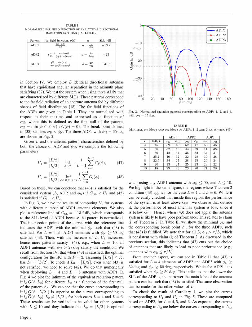
TABLE INORMALIZED FAR FIELD FUNCTION OF ANALYTICAL DIRECTIONAL
RADIATION PATTERNS [18, TABLE 2]
Pattern Far field function: g(φ) a SLL [dB]ADP1 sin(aφ)
aφa = π
φN−13.2
ADP2 (π2
)2cos(aφ)
(π2)2−(aφ)2
a = 3π2φN
−23
ADP3 π2
aφsin(aφ)
(π)2−(aφ)2a = 2π
φN−31.5
in Section IV. We employ L identical directional antennasthat have equidistant angular separation in the azimuth planesatisfying (37). We test the system when using three ADPs thatare characterized by different SLLs. These patterns correspondto the far field radiation of an aperture antenna fed by differentshapes of field distribution [18]. The far field functions ofthe ADPs are given in Table I. They are normalized withrespect to their maxima and expressed as a function ofφN, where this is defined as the first null of the pattern,φN = minφ ∈ [0, π) : G(φ) = 0. The break point definedin (38) satisfies φB < φN. The three ADPs with φN = 65 degare shown in Fig. 2.
Given L and the antenna pattern characteristics defined byboth the choice of ADP and φN, we compute the followingparameters
U1 =bL/2cdL/2e
infφ∈J
1
L− 1
L−2∑l=0
Gl(φ), (47)
U2 =bL/2cdL/2e
infφ∈[0,2π/L)
1
L
L−1∑l=0
Gl(φ). (48)
Based on these, we can conclude that (43) is satisfied for theconsidered system (L, ADP, and φN) if GSL < U1 and (45)is satisfied if GSL < U2.
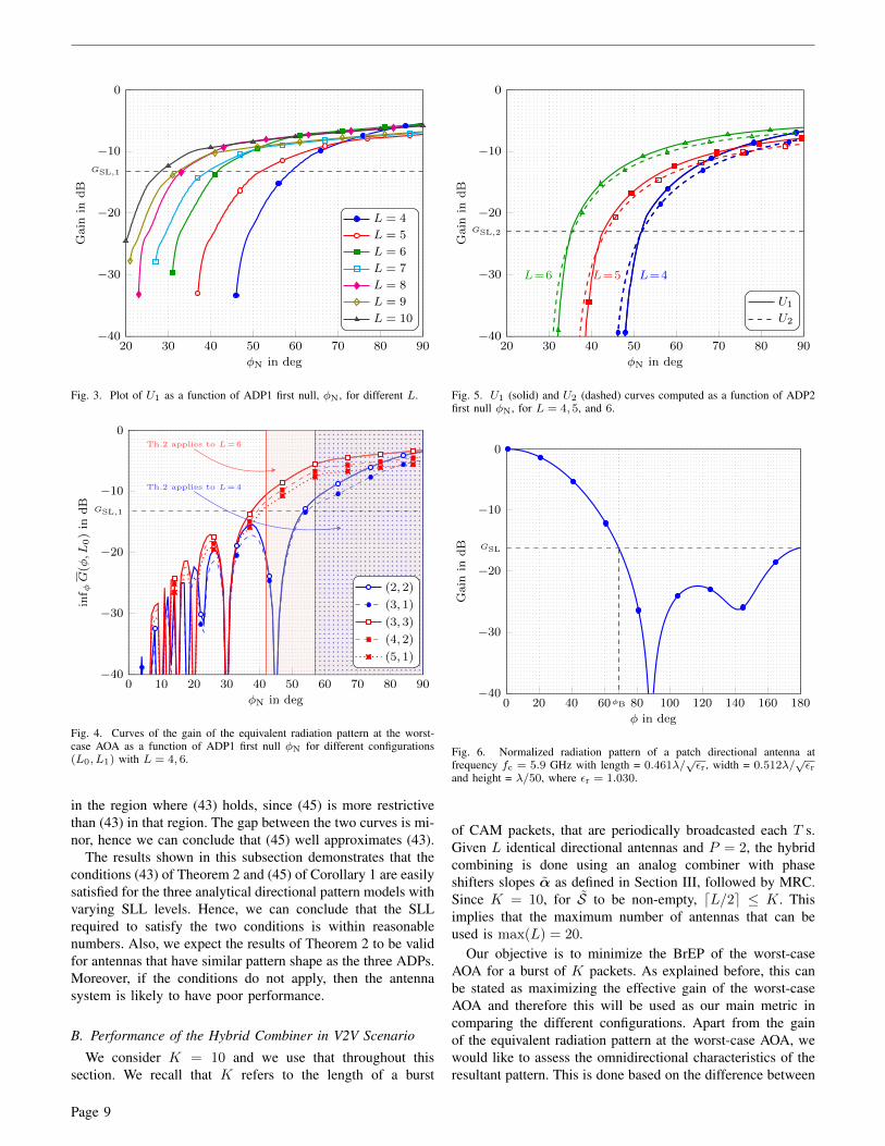
In Fig. 3, we have the results of computing U1 for systemswith different number of ADP1 antenna elements. We alsoplot a reference line of GSL = −13.2 dB, which correspondsto the SLL level of ADP1 because the pattern is normalized.The intersection points of the curves with the reference lineindicates the ADP1 with the minimal φN such that (43) issatisfied. For L = 4 all ADP1 antennas with φN ≥ 59 degsatisfies (43). Then, with the increase of L, U1 increases,hence more patterns satisfy (43), e.g., when L = 10, allADP1 antennas with φN > 28 deg satisfy the condition. Werecall from Section IV, that when (43) is satisfied, the optimalconfiguration for the HC with P = 2, assuming dL/2e ≤ K,has L0 = dL/2e. To check if L0 = dL/2e, even when (43) isnot satisfied, we need to solve (42). We do that numericallywhen deploying L = 4 and L = 6 antennas with ADP1. InFig. 4 we plot the infimum of the equivalent radiation patterninfφG(φ,L0) for different L0 as a function of the first nullof the pattern φN. We can see that the curve corresponding toinfφG(φ, dL/2e) is superior to the curves corresponding toinfφG(φ,L0), L0 6= dL/2e, for both cases L = 4 and L = 6.These results can be verified to be valid for other systemswith L ≤ 10 and they indicate that L0 = dL/2e is optimal
0 20 40 60 80 100 120 140 160 180−40
−30
−20
−10
0
GSL,1
GSL,2
GSL,3
φ in deg
Gain
indB
ADP1
ADP2
ADP3
Fig. 2. Normalized radiation patterns corresponding to ADPs 1, 2, and 3,with φN = 65 deg.
TABLE IIMINIMAL φN (deg) AND φB (deg) OF ADPS 1, 2 AND 3 SATISFYING (43)
ADP1 ADP2 ADP3L 180/L φN φB φN φB φN φB4 45 59 48 52 47 50 465 36 52 42 43 39 41 386 30 42 34 36 32 34 317 25.7 40 32 32 28 30 288 22.5 34 27 28 25 26 249 20 33 27 25 23 23 2210 18 29 23 23 20 21 20
when using any ADP1 antenna with φN ≤ 90, and L ≤ 10.We highlight in the same figure, the regions where Theorem 2condition (43) applies for the case L = 4 and L = 6. While itcan be easily checked that inside this region, the performanceof the system is at least above GSL, we observe that outsideit, the performance of most antennas system is low, since itis below GSL. Hence, when (43) does not apply, the antennasystem is likely to have poor performance. This relates to claim(i) of Theorem 2. In Table II, we show the minimal φN andthe corresponding break point φB for the three ADPs, suchthat (43) is fulfilled. We note that for all L, φB > π/L, whichis consistent with claim (i) of Theorem 2. As discussed in theprevious section, this indicates that (43) cuts out the choiceof antennas that are likely to lead to poor performance (e.g.,antennas with φB ≤ π/L).
From another aspect, we can see in Table II that (43) issatisfied for L = 4 elements of ADP2 and ADP3 with φN ≥52 deg and φN ≥ 50 deg, respectively. While for ADP1 it issatisfied when φN ≥ 59 deg. This indicates that the lower theSLL of the ADP is, the narrower the main lobe of the antennapattern can be, such that (43) is satisfied. The same observationcan be made for the other values of L.
To check the result of Corollary 1, we plot the curvescorresponding to U1 and U2 in Fig. 5. These are computedbased on ADP2, for L = 4, 5, and 6. As expected, the curvescorresponding to U2 are below the curves corresponding to U1,
Page 8
20 30 40 50 60 70 80 90−40
−30
−20
−10
0
GSL,1
φN in deg
Gain
indB
L = 4
L = 5
L = 6
L = 7
L = 8
L = 9
L = 10
Fig. 3. Plot of U1 as a function of ADP1 first null, φN, for different L.
0 10 20 30 40 50 60 70 80 90−40
−30
−20
−10
0
GSL,1
Th.2 applies to L=6
Th.2 applies to L=4
φN in deg
inf φ
G(φ
,L0)in
dB
(2, 2)
(3, 1)
(3, 3)
(4, 2)
(5, 1)
Fig. 4. Curves of the gain of the equivalent radiation pattern at the worst-case AOA as a function of ADP1 first null φN for different configurations(L0, L1) with L = 4, 6.
in the region where (43) holds, since (45) is more restrictivethan (43) in that region. The gap between the two curves is mi-nor, hence we can conclude that (45) well approximates (43).
The results shown in this subsection demonstrates that theconditions (43) of Theorem 2 and (45) of Corollary 1 are easilysatisfied for the three analytical directional pattern models withvarying SLL levels. Hence, we can conclude that the SLLrequired to satisfy the two conditions is within reasonablenumbers. Also, we expect the results of Theorem 2 to be validfor antennas that have similar pattern shape as the three ADPs.Moreover, if the conditions do not apply, then the antennasystem is likely to have poor performance.
B. Performance of the Hybrid Combiner in V2V Scenario
We consider K = 10 and we use that throughout thissection. We recall that K refers to the length of a burst
20 30 40 50 60 70 80 90−40
−30
−20
−10
0
GSL,2
L=4L=5L=6
φN in deg
Gain
indB
U1
U2
Fig. 5. U1 (solid) and U2 (dashed) curves computed as a function of ADP2first null φN, for L = 4, 5, and 6.
0 20 40 60 80 100 120 140 160 180−40
−30
−20
−10
0
φB
GSL
φ in deg
Gain
indB
Fig. 6. Normalized radiation pattern of a patch directional antenna atfrequency fc = 5.9 GHz with length = 0.461λ/
√εr, width = 0.512λ/
√εr
and height = λ/50, where εr = 1.030.
of CAM packets, that are periodically broadcasted each T s.Given L identical directional antennas and P = 2, the hybridcombining is done using an analog combiner with phaseshifters slopes α as defined in Section III, followed by MRC.Since K = 10, for S to be non-empty, dL/2e ≤ K. Thisimplies that the maximum number of antennas that can beused is max(L) = 20.
Our objective is to minimize the BrEP of the worst-caseAOA for a burst of K packets. As explained before, this canbe stated as maximizing the effective gain of the worst-caseAOA and therefore this will be used as our main metric incomparing the different configurations. Apart from the gainof the equivalent radiation pattern at the worst-case AOA, wewould like to assess the omnidirectional characteristics of theresultant pattern. This is done based on the difference between
Page 9
the highest and lowest gain of the equivalent pattern in dB,
R(L0) = 10 log10
supφG(φ,L0)
infφG(φ,L0). (49)
We use a patch antenna for our computations. These are low-profile antennas that are characterized by directional patterns.They are cheap to manufacture and can be integrated intomultiple positions on the vehicle [9, Ch. 4.1]. Hence, theyare suitable for vehicular multiple antenna systems. The nor-malized analytical pattern of the patch antenna used is shownin Fig. 6. The normalization is performed with respect tothe maximum directive gain of 9.21 dBi. The highest sidelobegain of the normalized pattern is GSL = −16.15 dB and thecorresponding break point is φB ≈ 69 deg.
We start by testing the performance of a system with L = 6.The antennas are distributed around the azimuth plan withuniform separation of 2π/L according to (37). To know whichconfiguration is optimal, we use the results of Theorem 2 orCorollary 1. We check here both conditions (43) and (45)by computing U1 and U2, which are given by (47) and (48),respectively. We get that U1 = −6.86 dB and U2 = −7.63 dB.Since GSL = −16.15 dB < U2 < U1, then we conclude thatthe optimal configuration has (L0, L1) = (3, 3). It can berepresented as S = [s0, s1] with s0 = [1, 1, 1, 0, 0, 0]T ands1 = [0, 0, 0, 1, 1, 1]T. The analog part of the HC is realizedusing
α0(S) = [α0,0, α1,0, α2,0]T = [0,2π
KT,
4π
KT]T,
α1(S) = [α3,1, α4,1, α5,1]T = [0,2π
KT,
4π
KT]T.
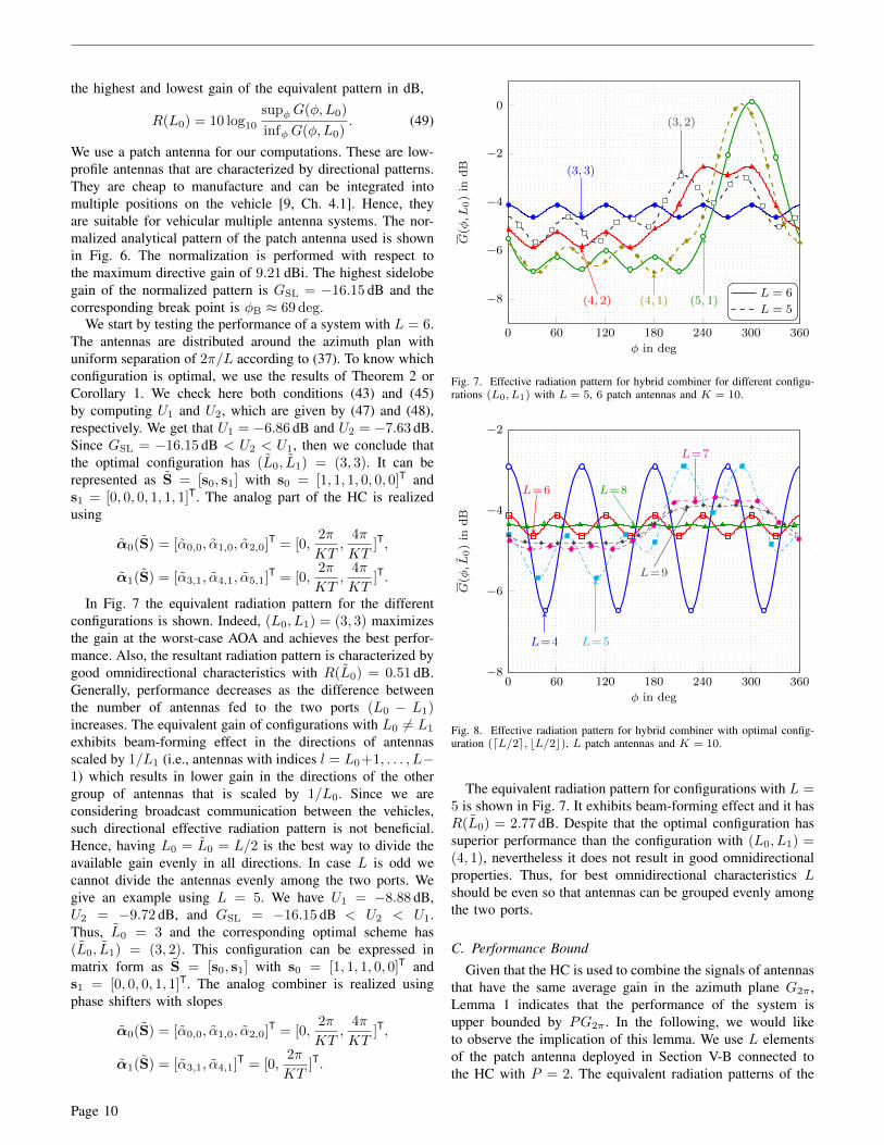
In Fig. 7 the equivalent radiation pattern for the differentconfigurations is shown. Indeed, (L0, L1) = (3, 3) maximizesthe gain at the worst-case AOA and achieves the best perfor-mance. Also, the resultant radiation pattern is characterized bygood omnidirectional characteristics with R(L0) = 0.51 dB.Generally, performance decreases as the difference betweenthe number of antennas fed to the two ports (L0 − L1)increases. The equivalent gain of configurations with L0 6= L1
exhibits beam-forming effect in the directions of antennasscaled by 1/L1 (i.e., antennas with indices l = L0+1, . . . , L−1) which results in lower gain in the directions of the othergroup of antennas that is scaled by 1/L0. Since we areconsidering broadcast communication between the vehicles,such directional effective radiation pattern is not beneficial.Hence, having L0 = L0 = L/2 is the best way to divide theavailable gain evenly in all directions. In case L is odd wecannot divide the antennas evenly among the two ports. Wegive an example using L = 5. We have U1 = −8.88 dB,U2 = −9.72 dB, and GSL = −16.15 dB < U2 < U1.Thus, L0 = 3 and the corresponding optimal scheme has(L0, L1) = (3, 2). This configuration can be expressed inmatrix form as S = [s0, s1] with s0 = [1, 1, 1, 0, 0]T ands1 = [0, 0, 0, 1, 1]T. The analog combiner is realized usingphase shifters with slopes
α0(S) = [α0,0, α1,0, α2,0]T = [0,2π
KT,
4π
KT]T,
α1(S) = [α3,1, α4,1]T = [0,2π
KT]T.
0 60 120 180 240 300 360
−8
−6
−4
−2
0
(5, 1)(4, 2) (4, 1)
(3, 3)
(3, 2)
φ in deg
G(φ
,L0)in
dB
L = 6
L = 5
Fig. 7. Effective radiation pattern for hybrid combiner for different configu-rations (L0, L1) with L = 5, 6 patch antennas and K = 10.
0 60 120 180 240 300 360−8
−6
−4
−2
L=4
L=6 L=8
L=5
L=7
L=9
φ in deg
G(φ
,L0)in
dB
Fig. 8. Effective radiation pattern for hybrid combiner with optimal config-uration (dL/2e, bL/2c), L patch antennas and K = 10.
The equivalent radiation pattern for configurations with L =5 is shown in Fig. 7. It exhibits beam-forming effect and it hasR(L0) = 2.77 dB. Despite that the optimal configuration hassuperior performance than the configuration with (L0, L1) =(4, 1), nevertheless it does not result in good omnidirectionalproperties. Thus, for best omnidirectional characteristics Lshould be even so that antennas can be grouped evenly amongthe two ports.
C. Performance Bound
Given that the HC is used to combine the signals of antennasthat have the same average gain in the azimuth plane G2π ,Lemma 1 indicates that the performance of the system isupper bounded by PG2π . In the following, we would liketo observe the implication of this lemma. We use L elementsof the patch antenna deployed in Section V-B connected tothe HC with P = 2. The equivalent radiation patterns of the
Page 10
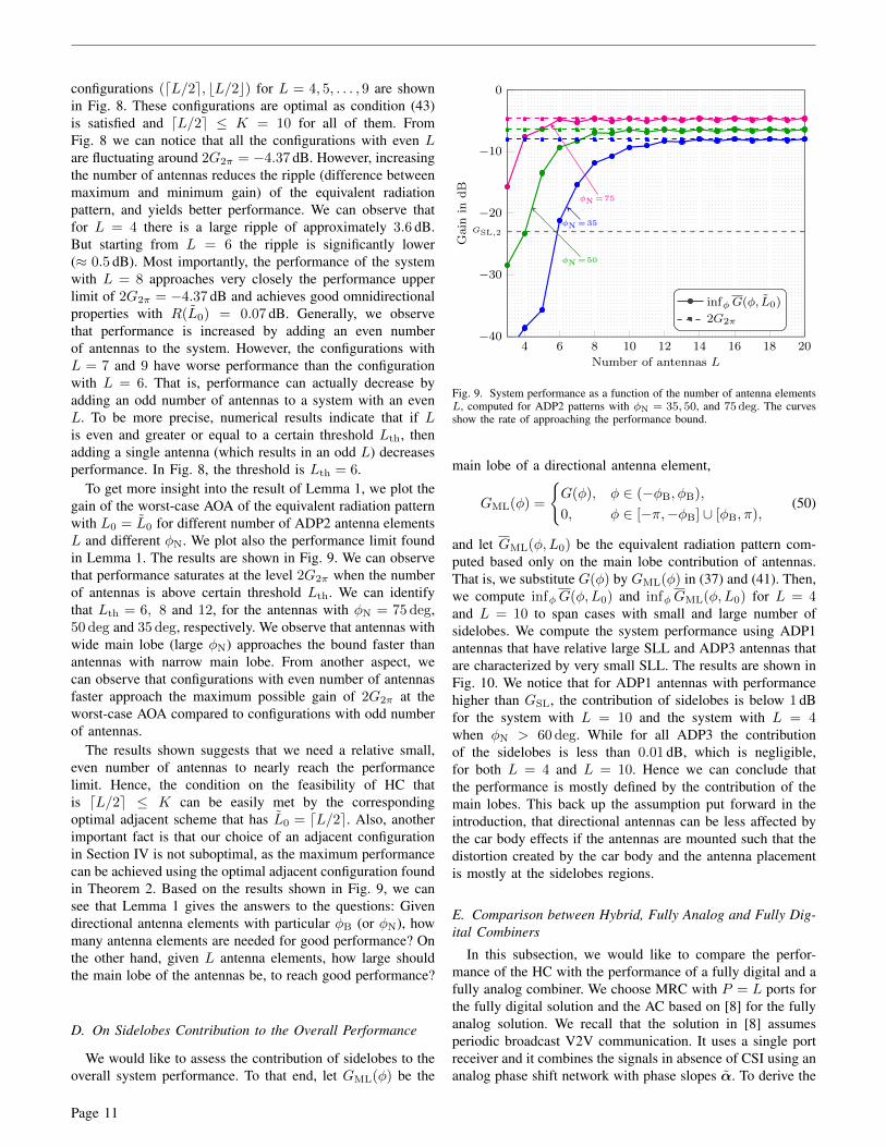
configurations (dL/2e, bL/2c) for L = 4, 5, . . . , 9 are shownin Fig. 8. These configurations are optimal as condition (43)is satisfied and dL/2e ≤ K = 10 for all of them. FromFig. 8 we can notice that all the configurations with even Lare fluctuating around 2G2π = −4.37 dB. However, increasingthe number of antennas reduces the ripple (difference betweenmaximum and minimum gain) of the equivalent radiationpattern, and yields better performance. We can observe thatfor L = 4 there is a large ripple of approximately 3.6 dB.But starting from L = 6 the ripple is significantly lower(≈ 0.5 dB). Most importantly, the performance of the systemwith L = 8 approaches very closely the performance upperlimit of 2G2π = −4.37 dB and achieves good omnidirectionalproperties with R(L0) = 0.07 dB. Generally, we observethat performance is increased by adding an even numberof antennas to the system. However, the configurations withL = 7 and 9 have worse performance than the configurationwith L = 6. That is, performance can actually decrease byadding an odd number of antennas to a system with an evenL. To be more precise, numerical results indicate that if Lis even and greater or equal to a certain threshold Lth, thenadding a single antenna (which results in an odd L) decreasesperformance. In Fig. 8, the threshold is Lth = 6.
To get more insight into the result of Lemma 1, we plot thegain of the worst-case AOA of the equivalent radiation patternwith L0 = L0 for different number of ADP2 antenna elementsL and different φN. We plot also the performance limit foundin Lemma 1. The results are shown in Fig. 9. We can observethat performance saturates at the level 2G2π when the numberof antennas is above certain threshold Lth. We can identifythat Lth = 6, 8 and 12, for the antennas with φN = 75 deg,50 deg and 35 deg, respectively. We observe that antennas withwide main lobe (large φN) approaches the bound faster thanantennas with narrow main lobe. From another aspect, wecan observe that configurations with even number of antennasfaster approach the maximum possible gain of 2G2π at theworst-case AOA compared to configurations with odd numberof antennas.
The results shown suggests that we need a relative small,even number of antennas to nearly reach the performancelimit. Hence, the condition on the feasibility of HC thatis dL/2e ≤ K can be easily met by the correspondingoptimal adjacent scheme that has L0 = dL/2e. Also, anotherimportant fact is that our choice of an adjacent configurationin Section IV is not suboptimal, as the maximum performancecan be achieved using the optimal adjacent configuration foundin Theorem 2. Based on the results shown in Fig. 9, we cansee that Lemma 1 gives the answers to the questions: Givendirectional antenna elements with particular φB (or φN), howmany antenna elements are needed for good performance? Onthe other hand, given L antenna elements, how large shouldthe main lobe of the antennas be, to reach good performance?
D. On Sidelobes Contribution to the Overall Performance
We would like to assess the contribution of sidelobes to theoverall system performance. To that end, let GML(φ) be the
4 6 8 10 12 14 16 18 20−40
−30
−20
−10
0
GSL,2
φN =35
φN =50
φN =75
Number of antennas L
Gain
indB
infφ G(φ, L0)
2G2π
Fig. 9. System performance as a function of the number of antenna elementsL, computed for ADP2 patterns with φN = 35, 50, and 75 deg. The curvesshow the rate of approaching the performance bound.
main lobe of a directional antenna element,
GML(φ) =
G(φ), φ ∈ (−φB, φB),
0, φ ∈ [−π,−φB] ∪ [φB, π),(50)
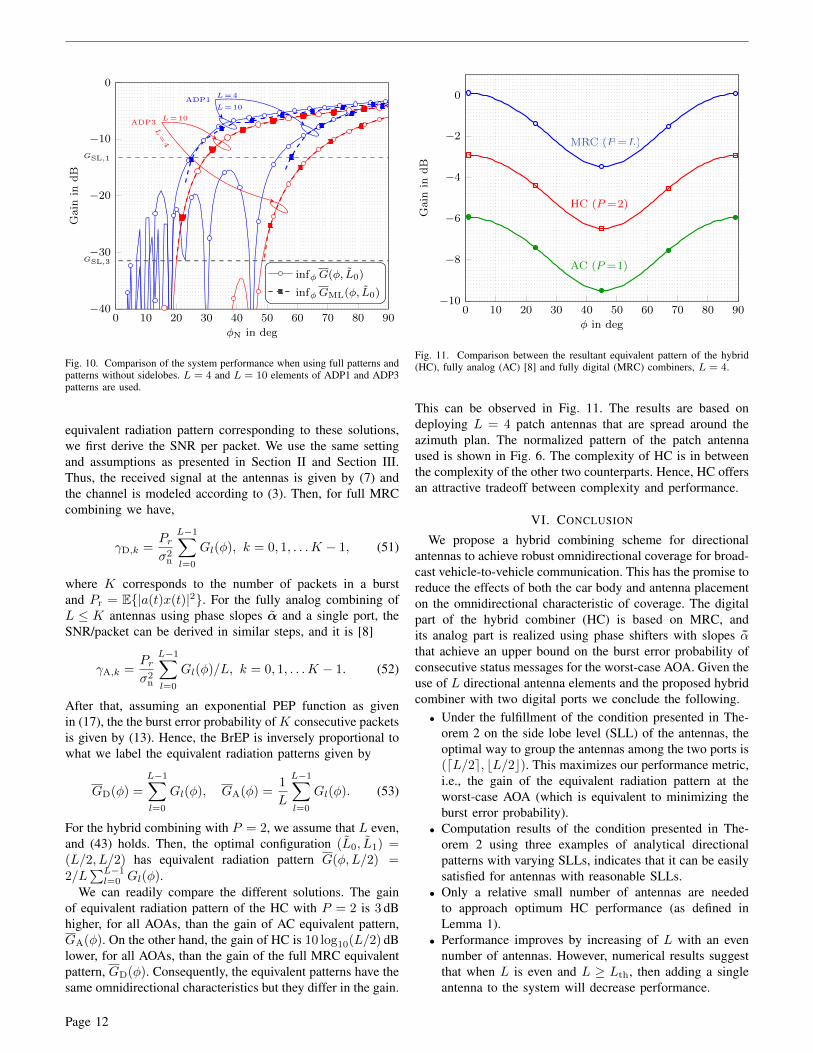
and let GML(φ,L0) be the equivalent radiation pattern com-puted based only on the main lobe contribution of antennas.That is, we substitute G(φ) by GML(φ) in (37) and (41). Then,we compute infφG(φ,L0) and infφGML(φ,L0) for L = 4and L = 10 to span cases with small and large number ofsidelobes. We compute the system performance using ADP1antennas that have relative large SLL and ADP3 antennas thatare characterized by very small SLL. The results are shown inFig. 10. We notice that for ADP1 antennas with performancehigher than GSL, the contribution of sidelobes is below 1 dBfor the system with L = 10 and the system with L = 4when φN > 60 deg. While for all ADP3 the contributionof the sidelobes is less than 0.01 dB, which is negligible,for both L = 4 and L = 10. Hence we can conclude thatthe performance is mostly defined by the contribution of themain lobes. This back up the assumption put forward in theintroduction, that directional antennas can be less affected bythe car body effects if the antennas are mounted such that thedistortion created by the car body and the antenna placementis mostly at the sidelobes regions.
E. Comparison between Hybrid, Fully Analog and Fully Dig-ital Combiners
In this subsection, we would like to compare the perfor-mance of the HC with the performance of a fully digital and afully analog combiner. We choose MRC with P = L ports forthe fully digital solution and the AC based on [8] for the fullyanalog solution. We recall that the solution in [8] assumesperiodic broadcast V2V communication. It uses a single portreceiver and it combines the signals in absence of CSI using ananalog phase shift network with phase slopes α. To derive the
Page 11
0 10 20 30 40 50 60 70 80 90−40
−30
−20
−10
0
GSL,1
GSL,3
ADP3L=10
L=
4
ADP1L=4
L=10
φN in deg
Gain
indB
infφ G(φ, L0)
infφ GML(φ, L0)
Fig. 10. Comparison of the system performance when using full patterns andpatterns without sidelobes. L = 4 and L = 10 elements of ADP1 and ADP3patterns are used.
equivalent radiation pattern corresponding to these solutions,we first derive the SNR per packet. We use the same settingand assumptions as presented in Section II and Section III.Thus, the received signal at the antennas is given by (7) andthe channel is modeled according to (3). Then, for full MRCcombining we have,
γD,k =Prσ2
n
L−1∑l=0
Gl(φ), k = 0, 1, . . .K − 1, (51)
where K corresponds to the number of packets in a burstand Pr = E|a(t)x(t)|2. For the fully analog combining ofL ≤ K antennas using phase slopes α and a single port, theSNR/packet can be derived in similar steps, and it is [8]
γA,k =Prσ2
n
L−1∑l=0
Gl(φ)/L, k = 0, 1, . . .K − 1. (52)
After that, assuming an exponential PEP function as givenin (17), the the burst error probability of K consecutive packetsis given by (13). Hence, the BrEP is inversely proportional towhat we label the equivalent radiation patterns given by
GD(φ) =
L−1∑l=0
Gl(φ), GA(φ) =1
L
L−1∑l=0
Gl(φ). (53)
For the hybrid combining with P = 2, we assume that L even,and (43) holds. Then, the optimal configuration (L0, L1) =(L/2, L/2) has equivalent radiation pattern G(φ,L/2) =2/L
∑L−1l=0 Gl(φ).
We can readily compare the different solutions. The gainof equivalent radiation pattern of the HC with P = 2 is 3 dBhigher, for all AOAs, than the gain of AC equivalent pattern,GA(φ). On the other hand, the gain of HC is 10 log10(L/2) dBlower, for all AOAs, than the gain of the full MRC equivalentpattern, GD(φ). Consequently, the equivalent patterns have thesame omnidirectional characteristics but they differ in the gain.
0 10 20 30 40 50 60 70 80 90−10
−8
−6
−4
−2
0
MRC (MRC (MRC (PP ==LL))
HC (P =2)
AC (P =1)
φ in deg
Gain
indB
Fig. 11. Comparison between the resultant equivalent pattern of the hybrid(HC), fully analog (AC) [8] and fully digital (MRC) combiners, L = 4.
This can be observed in Fig. 11. The results are based ondeploying L = 4 patch antennas that are spread around theazimuth plan. The normalized pattern of the patch antennaused is shown in Fig. 6. The complexity of HC is in betweenthe complexity of the other two counterparts. Hence, HC offersan attractive tradeoff between complexity and performance.
VI. CONCLUSION
We propose a hybrid combining scheme for directionalantennas to achieve robust omnidirectional coverage for broad-cast vehicle-to-vehicle communication. This has the promise toreduce the effects of both the car body and antenna placementon the omnidirectional characteristic of coverage. The digitalpart of the hybrid combiner (HC) is based on MRC, andits analog part is realized using phase shifters with slopes αthat achieve an upper bound on the burst error probability ofconsecutive status messages for the worst-case AOA. Given theuse of L directional antenna elements and the proposed hybridcombiner with two digital ports we conclude the following.• Under the fulfillment of the condition presented in The-
orem 2 on the side lobe level (SLL) of the antennas, theoptimal way to group the antennas among the two ports is(dL/2e, bL/2c). This maximizes our performance metric,i.e., the gain of the equivalent radiation pattern at theworst-case AOA (which is equivalent to minimizing theburst error probability).
• Computation results of the condition presented in The-orem 2 using three examples of analytical directionalpatterns with varying SLLs, indicates that it can be easilysatisfied for antennas with reasonable SLLs.
• Only a relative small number of antennas are neededto approach optimum HC performance (as defined inLemma 1).
• Performance improves by increasing of L with an evennumber of antennas. However, numerical results suggestthat when L is even and L ≥ Lth, then adding a singleantenna to the system will decrease performance.
Page 12

• To best approach the performance bound and for bestomnidirectional characteristics of the equivalent radiationpattern, the number of directional elements per portshould be the same, and thus L should be even.
• The HC uses (L−2) less ports than full MRC combiningto achieve an equivalent radiation pattern with a similaromnidirectional properties when L is even. However, theHC gain is 10 log10(L/2) dB less than full MRC (for anyAOA).
APPENDIX APROOF OF LEMMA 1
Proof. Let G(φ,S) defined as in (29), and let the averageradiation of all antennas in the azimuth plane be the same,
1
2π
∫2π
|gl(φ)|2dφ = G2π, ∀l. (54)
Then, it is easy to check that
1
2π
∫2π
G(φ,S)dφ = PG2π, S ∈ S. (55)
By the monotonicity of Riemann integral it follows that∫2π
infφ∈[0,2π)
G(φ,S)dφ ≤∫
2π
G(φ,S)dφ, S ∈ S. (56)
Thus, we can deduce that
infφ∈[0,2π)
G(φ,S) ≤ PG2π, S ∈ S. (57)
By definition (32), S ∈ S . Replacing S by S in the previousequation, (36) follows.
APPENDIX BPROOF OF THEOREM 2
Proof. We start by fixing L and defining the function
fN (φ) ,L−1∑l=N
Gl(φ), N = 0, 1, . . . , L− 1, (58)
where Gl(φ) = G(φ − l2π/L) and G(φ) is as defined as inTheorem 2. We specifically recall that φB < π/2.
We can divide Gl(φ) into main lobe regions and sidelobesregions. The principal main lobe region for Gl(φ) is definedas
Ll ,(l2π/L− φB, l2π/L+ φB
), l ∈ Z. (59)
Clearly, Gl(φ) > GSL for φ ∈ Ll. In fact, since Gl(φ) isperiodic with period 2π, Gl(φ) > GSL for φ ∈ Ll+nL for anyinteger n. Since adjacent antennas are spaced with 2π/L, theirprincipal main lobe regions will overlap when φB > π/L, i.e.,
(φB > π/L)⇔ (inf Ll < supLl−1). (60)
We note that fN (φ) is periodic with period 2π, and we willstudy its properties in the following interval of length 2π,
I , [supL−1, supLL−1). (61)
We define
Ic0(N) , (inf LN , supLL−1), N = 0, 1, . . . , L− 1, (62)
and
I0(N) , I \ Ic0(N), N = 0, 1, . . . , L− 1, (63)
= [supL−1, inf LN ], N = 0, 1, . . . , L− 1. (64)
Hence, the principal main lobes of the Gl(φ) terms constitut-ing fN (φ) are contained in Ic
0(N), that is
Ll ⊆ Ic0(N), l = N, . . . , L− 1. (65)
Conversely, the Gl(φ) terms in fN (φ) have only sidelobescontributions in I0(N). The combinations of φB and N thatimply that I0(N) 6= ∅ are characterized by the followinglemma.
Lemma 2. Let
nB , LφB/π − 1, (66)
M , m ∈ N : dnBe ≤ m ≤ L− 1, (67)
where N = 0, 1, 2, . . .. Then the following conditions areequivalent
(I0(N) 6= ∅)⇔ (N ∈M). (68)
Proof. We see from the definitions (61), (62), and (63) thatI0(N) is nonempty if, and only if, inf LN ≥ supL−1, i.e., if(N(2π/L)− φB ≥ −(2π/L) + φB). The latter condition canbe rewritten as N ≥ nB or, since N ≤ L−1, as N ∈M.
From the above lemma and (65), we conclude that the termsin fN (φ) can be bounded as
Gl(φ) ≤ GSL, φ ∈ I0(N), N ≤ l ≤ L− 1, N ∈M. (69)
We can now restate the main condition for the theorem (43)by noting that J = I0(L− 1), as
GSL <bL/2cdL/2e
infφ∈I0(L−1)
1
L− 1
L−2∑l=0
Gl(φ). (70)
Lemma 3. If (70) holds then φB > πL .
Proof. We will use a proof of contradiction, i.e., we assumethat (70) holds and φB ≤ π/L and derive a contradiction.
If φB ≤ π/L, then nB ≤ 0 and thus 0 ∈ M, where nB
and M are defined according to (66) and (67), respectively.By Lemma 2, I0(0) 6= ∅, then (69) implies that
GSL ≥ infφ∈I0(0)
1
L− 1
L−2∑l=0
Gl(φ) (71)
≥ infφ∈I0(L−1)
1
L− 1
L−2∑l=0
Gl(φ), (72)
where the last inequality holds since I0(0) ⊂ I0(L− 1).If (70) holds and since bL/2c/dL/2e ≤ 1 then
GSL < infφ∈I0(L−1)
1
L− 1
L−2∑l=0
Gl(φ), (73)
which contradicts (72) and the lemma follows.
The above lemma proves claim (i) of the theorem. Followingthis result, we can assume φB > π/L for the remainder of theproof.
Page 13
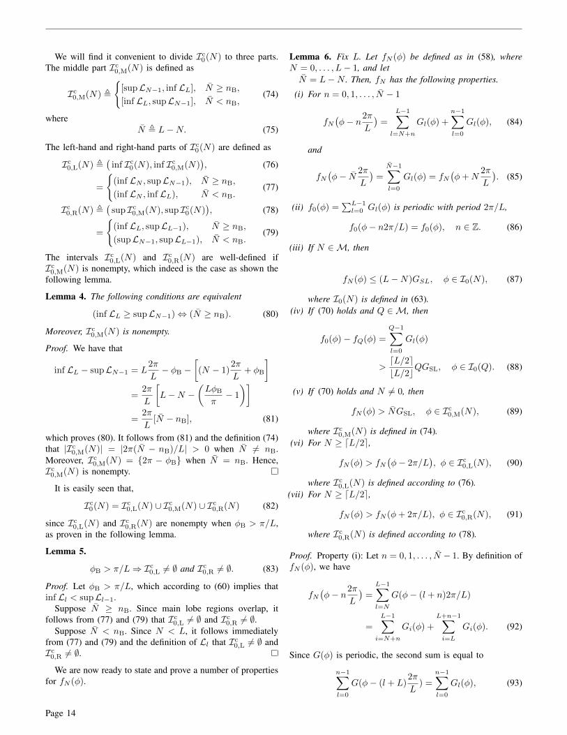
We will find it convenient to divide Ic0(N) to three parts.
The middle part Ic0,M(N) is defined as
Ic0,M(N) ,
[supLN−1, inf LL], N ≥ nB,
[inf LL, supLN−1], N < nB,(74)
whereN , L−N. (75)
The left-hand and right-hand parts of Ic0(N) are defined as
Ic0,L(N) ,
(inf Ic
0(N), inf Ic0,M(N)
), (76)
=
(inf LN , supLN−1), N ≥ nB,
(inf LN , inf LL), N < nB.(77)
Ic0,R(N) ,
(sup Ic
0,M(N), sup Ic0(N)
), (78)
=
(inf LL, supLL−1), N ≥ nB,
(supLN−1, supLL−1), N < nB.(79)
The intervals Ic0,L(N) and Ic
0,R(N) are well-defined ifIc
0,M(N) is nonempty, which indeed is the case as shown thefollowing lemma.
Lemma 4. The following conditions are equivalent
(inf LL ≥ supLN−1)⇔ (N ≥ nB). (80)
Moreover, Ic0,M(N) is nonempty.
Proof. We have that
inf LL − supLN−1 = L2π
L− φB −
[(N − 1)
2π
L+ φB
]=
2π
L
[L−N −
(LφB
π− 1
)]=
2π
L[N − nB], (81)
which proves (80). It follows from (81) and the definition (74)that |Ic
0,M(N)| = |2π(N − nB)/L| > 0 when N 6= nB.Moreover, Ic
0,M(N) = 2π − φB when N = nB. Hence,Ic
0,M(N) is nonempty.
It is easily seen that,
Ic0(N) = Ic
0,L(N) ∪ Ic0,M(N) ∪ Ic
0,R(N) (82)
since Ic0,L(N) and Ic
0,R(N) are nonempty when φB > π/L,as proven in the following lemma.
Lemma 5.
φB > π/L⇒ Ic0,L 6= ∅ and Ic
0,R 6= ∅. (83)
Proof. Let φB > π/L, which according to (60) implies thatinf Ll < supLl−1.
Suppose N ≥ nB. Since main lobe regions overlap, itfollows from (77) and (79) that Ic
0,L 6= ∅ and Ic0,R 6= ∅.
Suppose N < nB. Since N < L, it follows immediatelyfrom (77) and (79) and the definition of Ll that Ic
0,L 6= ∅ andIc
0,R 6= ∅.
We are now ready to state and prove a number of propertiesfor fN (φ).
Lemma 6. Fix L. Let fN (φ) be defined as in (58), whereN = 0, . . . , L− 1, and letN = L−N . Then, fN has the following properties.
(i) For n = 0, 1, . . . , N − 1
fN(φ− n2π
L
)=
L−1∑l=N+n
Gl(φ) +
n−1∑l=0
Gl(φ), (84)
and
fN(φ− N 2π
L
)=
N−1∑l=0
Gl(φ) = fN(φ+N
2π
L
). (85)
(ii) f0(φ) =∑L−1l=0 Gl(φ) is periodic with period 2π/L,
f0(φ− n2π/L) = f0(φ), n ∈ Z. (86)
(iii) If N ∈M, then
fN (φ) ≤ (L−N)GSL, φ ∈ I0(N), (87)
where I0(N) is defined in (63).(iv) If (70) holds and Q ∈M, then
f0(φ)− fQ(φ) =
Q−1∑l=0
Gl(φ)
>dL/2ebL/2c
QGSL, φ ∈ I0(Q). (88)
(v) If (70) holds and N 6= 0, then
fN (φ) > NGSL, φ ∈ Ic0,M(N), (89)
where Ic0,M(N) is defined in (74).
(vi) For N ≥ dL/2e,
fN (φ) > fN(φ− 2π/L
), φ ∈ Ic
0,L(N), (90)
where Ic0,L(N) is defined according to (76).
(vii) For N ≥ dL/2e,
fN (φ) > fN (φ+ 2π/L), φ ∈ Ic0,R(N), (91)
where Ic0,R(N) is defined according to (78).
Proof. Property (i): Let n = 0, 1, . . . , N − 1. By definition offN (φ), we have
fN(φ− n2π
L
)=
L−1∑l=N
G(φ− (l + n)2π/L)
=
L−1∑i=N+n
Gi(φ) +
L+n−1∑i=L
Gi(φ). (92)
Since G(φ) is periodic, the second sum is equal to
n−1∑l=0
G(φ− (l + L)2π
L) =
n−1∑l=0
Gl(φ), (93)
Page 14
13 73 133 193 253 313 3730
0.2
0.4
0.6
0.8
1
L0
LN−1
LN
LL−1
LL
I0(N) Ic0,L(N) Ic
0,M(N) Ic0,R(N)
Ic0(N)
φ in deg
Gain
(a) Case N ≥ nB, (N = 4)
13 73 133 193 253 313 3730
0.2
0.4
0.6
0.8
1
L0
LN−1
LL−1
LL
I0(N) Ic0,L(N)Ic
0,M(N)Ic0,R(N)
Ic0(N)
φ in deg
Gain
(b) Case N < nB, (N = 5)
Fig. 12. Illustration of the intervals I0(N), Ic0(N), Ic0,M(N), Ic0,R(N) and Ic0,L(N) for different cases, L = 6, φB = 73 deg.
which proves (84). To prove (85), we have
fN(φ− N 2π
L
)=
L−1∑l=N
G(φ− (l + L−N)2π/L)
=
L−1∑l=N
G(φ+N2π/L− l2π/L) (94)
=
N−1∑l=0
G(φ− l2π/L). (95)
From another aspect, (94) can be expressed as
L−1∑l=N
G(φ+N2π/L− l2π/L) = fN (φ+N2π/L). (96)
Putting this together with (95) proves (85) and the propertyfollows.
Property (ii): Let n = kL + n′, where n′, k ∈ Z and 0 ≤n′ ≤ (L− 1). Then,
f0
(φ− n2π/L
)= f0
(φ− n′2π/L
)(97)
=
L−1∑l=n′
Gl(φ) +
n′−1∑l=0
Gl(φ) (98)
= f0(φ), (99)
where (97) holds since f0 is periodic with period 2π, and (98)follows from (84) (since N = 0, n′ < N = L).
Property (iii): Follows directly from (69).Property (iv): By assumption (70) holds. It implies that
(L−1)−1∑l=0
Gl(φ) > a(L− 1)GSL, φ ∈ I0(L− 1), (100)
where a = dL/2e/bL/2c ≥ 1. Hence the property holds forQ = L− 1. Now, let Q < L− 1, then for φ ∈ I0(L− 1),Q−1∑l=0
Gl(φ) =
L−2∑l=0
Gl(φ)−L−2∑l=Q
Gl(φ)
> a(L− 1)GSL −L−2∑l=Q
Gl(φ) (101)
= aQGSL + a(L− 1−Q)GSL −L−2∑l=Q
Gl(φ),
(102)
where (101) follows from (100). Since Q < L− 1, it followsfrom the definition of I0(N) that I0(Q) ⊂ I0(L− 1). Hence,(102) holds in particular for φ ∈ I0(Q). What remains is toshow that the sum of last two terms in (102) is nonnegative. Tothis end, let φ ∈ I0(Q). Then by (69), we have that Gl(φ) ≤GSL, for l = Q,Q+ 1, . . . , L− 1 and
a(L− 1−Q)GSL −L−2∑l=Q
Gl(φ)
≥ a(L− 1−Q)GSL − (L− 1−Q)GSL
= (a− 1)(L− 1−Q)GSL
≥ 0, (103)
since a ≥ 1, and the property follows.Property (v): Let N 6= 0, then N ≤ L − 1. Based on the
definition of Ic0,M(N) we divide the proof into two cases N ≥
nB and N < nB.We start tackling the case N ≥ nB. From (74) we
have Ic0,M(N) = [supLN−1, inf LL]. Since (70) holds and
nB ≤ N ≤ L− 1, that is N ∈ M, Lemma 6 property (iv) isapplicable with Q = N . We can use (85), (88), and the factthat dL/2e/bL/2c ≥ 1 to show
fN (φ′ +N2π/L) > NGSL, φ′ ∈ I0(N). (104)
Now if φ′ ∈ I0(N), then by definition,
−2π/L+ φB ≤ φ′ ≤ N2π/L− φB. (105)
Page 15

Adding N2π/L to the inequality sides we get,
φ′ +N2π/L ≥ (N − 1)2π/L+ φB
φ′ +N2π/L ≤ (N +N)2π/L− φB, (106)
which, since N +N = L, is equivalent to
supLN−1 ≤ φ′ +N2π/L ≤ inf LL.
Thus, if φ′ ∈ I0(N), then φ = (φ′+N2π/L) ∈ Ic0,M(N) and
(104) can be written as
fN (φ) > NGSL, φ ∈ Ic0,M(N), (107)
which proves the property for the case when N ≥ nB.We now move to the case N < nB where Ic
0,M(N) =[inf LL, supLN−1]. From the definition of Ll it follows thatfor l = N,N + 1, . . . L− 1,
inf Ic0,M(N) = inf LL > inf Ll (108)
sup Ic0,M(N) = supLN−1 < supLl, (109)
which implies that Ic0,M(N) ⊂ Ll for l = N,N + 1, . . . L− 1
and
fN (φ) =
L−1∑l=N
Gl(φ) > (L−N)GSL, φ ∈ Ic0,M(N).
(110)Hence, (89) holds when N < nB as well, and the propertyfollows.
Property (vi): We recall that φB > π/L, which impliesIc
0,R(N) 6= ∅ (Lemma 5). Using (84), we have that
fN (φ− 2π/L) =
L−1∑l=N+1
Gl(φ) +G0(φ), (111)
and
fN (φ)− fN (φ− 2π/L) = GN (φ)−G0(φ). (112)
From here, we prove (90) by showing that GN (φ) is a mainlobe term and G0(φ) is a sidelobes term when φ ∈ Ic
0,L(N).We demonstrate this for the two cases N ≥ nB and N < nB.
Let N ≥ nB. By definition (77), we have that Ic0,L(N) =
(inf LN , supLN−1). Since supLN−1 < supLN , we see thatIc
0,L(N) ⊂ LN , and
GN (φ) > GSL, φ ∈ Ic0,L(N). (113)
Then it is enough to show that G0(φ) ≤ GSL, when φ ∈Ic
0,L(N) for (90) to hold. This is equivalent to Ic0,L(N) ⊂
(supL0, inf LL). Since N ≥ dL/2e, and we recall that φB <π/2, then inf Ic
0,L(N) = N2π/L − φB ≥ π − φB > φB =supL0. Hence,
inf Ic0,L(N) > supL0. (114)
On the other hand, since N ≥ nB, then by (80)
sup Ic0,L(N) = supLN−1 ≤ inf LL, (115)
and thus we can conclude that G0(φ) ≤ GSL for φ ∈ Ic0,L(N),
and the property is proved for N ≥ nB.Now we proceed to the case N < nB. By definition we
have that Ic0,L(N) = (inf LN , inf LL). Then, again, since
N ≥ dL/2e, we have that inf Ic0,L(N) > supL0 and,
therefore, G0(φ) ≤ GSL for φ ∈ Ic0,L(N). Moreover, by (80),
we have inf LL < supLN−1 < supLN . Thus, it followsthat Ic
0,L(N) ⊂ LN and GN (φ) > GSL for φ ∈ Ic0,L(N).
Hence, (90) holds when N < nB as well and this ends theproof of the property.
Property (vii): Following the same steps as used toprove Property (vi), we can write fN (φ)− fN (φ+ 2π/L) =GL−1(φ) − GN−1(φ). Then we can deduce that Ic
0,R(N) ⊂LL−1 and Ic
0,R(N) ⊂ (supLN−1, inf LN−1 + 2π) and there-fore (91) holds.
Lemma 7. Let
L+ , l ∈ Z : L/2 < l ≤ L− 1. (116)
If L0 ∈ L+, then L0 ∈M.
Proof. We recall that π/L < φB < π/2. Let L0 ∈ L+. Wehave minM = dnBe = dLφB/πe − 1 < dL/2e − 1 < L/2 <L0. Hence, minM < L0 ≤ maxM, and the lemma follows.
Lemma 8. Let G(φ,L0) and I0(L0) be defined accordingto (41) and (63), respectively. If L0 ∈ L+ and (70) is satisfied,then
infφ∈[0,2π)
G(φ,L0) = infφ∈I0(L0)
G(φ,L0). (117)
Proof. Since G(φ,L0) is periodic and |I| = 2π,
φ0 = arg infφ∈[0,2π)
G(φ,L0) = arg infφ∈I
G(φ,L0), (118)
where I is defined in (61) and I = I0(L0) ∪ Ic0(L0),
where Ic0(L0) is defined according to (62). Hence, to prove
the lemma, it is sufficient to show that φ0 ∈ I0(L0) or,equivalently, that
φ0 /∈ Ic0(L0) (119)
since Ic0(L0) = I \ I0(L0).
We express G(φ,L0) in terms of fN (φ), where these aredefined according to (29) and (58), respectively, as
G(φ,L0) =(f0(φ) + bfL0
(φ))/L0, (120)
with b = (2L0 − L)/(L− L0) > 0.We note that Lemma 6 property (iv) and (v) holds in both
cases. Also, since L0 > L/2 implies that L0 ≥ dL/2e,Lemma 6 property (vi) and (vii) holds. Moreover, we knowfrom Lemma 7 that L0 ∈ M. Lastly, we recall that (70)implies φB > π/L (Lemma 3), and hence we let φB > π/Land proceed to show (119).
By (82) we have Ic0(L0) = Ic
0,L(L0)∪Ic0,M(L0)∪Ic
0,R(L0),where these intervals are nonempty and defined accordingto (76), (74) and (78), respectively. To prove (119), we usecontradictions to show that φ0 /∈ Ic
0,M(L0), φ0 /∈ Ic0,L(L0)
and φ0 /∈ Ic0,R(L0).
First, suppose φ0 ∈ Ic0,M(L0), Lemma 6 property (v) im-
plies
fL0(φ) > (L− L0)GSL, φ ∈ Ic
0,M(L0). (121)
Page 16
Substituting in (120) and taking into account the assumptionthat φ0 ∈ Ic
0,M(L0), we get
G(φ0, L0) >(f0(φ0) + (2L0 − L)GSL
)/L0. (122)
Now we attempt to find a φ′ /∈ Ic0,M(L0) such that
G(φ′, L0) < G(φ0, L0). Since L0 > L/2 then
|I0(L0)| = (L0 + 1)2π/L− 2φB > π + 2π/L− 2φB.
Recalling that φB < π/2, we get |I0(L0)| > 2π/L. Addingthat to the fact that f0(φ) is periodic with 2π/L (Lemma 6property (ii)), we deduce that ∃ φ′ ∈ I0(L0) such thatf0(φ′) = inf f0(φ). On the other hand, using Lemma 6property (iii) we have
fL0(φ) < (L− L0)GSL, φ ∈ I0(L0). (123)
Following this we can upper bound G(φ′, L0) as
G(φ′, L0) <(f0(φ′) + (2L0 − L)GSL
)/L0. (124)
Comparing (124) with (122) and taking into account the factthat f0(φ′) ≤ f0(φ0) we deduce that
G(φ′, L0) < G(φ0, L0). (125)
This contradicts the claim that the infimum of G(φ,L0), φ0 ∈Ic
0,M(L0), therefore φ0 /∈ Ic0,M(L0).
Secondly, suppose φ0 ∈ Ic0,R(L0), to find a contradiction to
this claim, we let φ′ = φ0 − 2π/L. By periodicity of f0(φ),we have that f0(φ′) = f0(φ0), then
G(φ′, L0) =(f0(φ0) + bfL0
(φ′))/L0. (126)
Moreover, by Lemma 6 property (vi) we have fL0(φ′) <
fL0(φ0). Therefore,
G(φ′, L0) <(f0(φ0) + bfL0(φ0)
)/L0 = G(φ0, L0). (127)
This is a contradiction. So we can conclude that φ0 /∈Ic
0,L(L0).Lastly, suppose φ0 ∈ Ic
0,R(L0), by similar argument to theprevious one, if we let φ′ = φ0 + 2π/L and use Lemma 6property (vii) we can deduce that G(φ′, L0) < G(φ0, L0) andthus φ0 /∈ Ic
0,R(L0).We have shown that if (70) holds then φ0 /∈ Ic
0,M(N), φ0 /∈Ic
0,R(N) and φ0 /∈ Ic0,L(N). Therefore, φ0 /∈ Ic
0(L0) and thisconcludes the proof of the Lemma.
Now we are set to show the main result of Theorem 2,i.e., claim (ii). We recall that claim (i) was already proven inLemma 3. By assumption, the gain of the highest sidelobesGSL satisfies (43), which is restated in (70). Then, we wantto prove that the solution to (42), with the constraint L0 ≤ Krelaxed, is (44), that is L0 = dL/2e, L1 = L− L0 = bL/2c.To prove this, it is enough to show that for L0 ∈ L+\dL/2e,
infφ∈[0,2π)
G(φ,L0) < infφ∈[0,2π)
G(φ, dL/2e), (128)
where G(φ,L0) is the equivalent radiation pattern givenby (41) and L+ is defined in (116).
We tackle the demonstration of (128) in two steps. In thefirst step we will show that for L0 ∈ L+ \ dL/2e,
infφ∈[0,2π)
G(φ,L0) < infφ∈I0(L0)
G(φ, dL/2e). (129)
And in the second step, we will demonstrate that
infφ∈[0,2π]
G(φ, dL/2e) = infφ∈I0(L0)
G(φ, dL/2e). (130)
We start the first step by forming
D(L0) = G(φ, dL/2e)−G(φ,L0)
=
(1
dL/2e− 1
L0
) dL/2e−1∑l=0
Gl(φ)
+
(1
bL/2c− 1
L0
) L0−1∑l=dL/2e
Gl(φ)
+
(1
bL/2c− 1
L− L0
) L−1∑l=L0
Gl(φ)
≥(
1
dL/2e− 1
L0
) L0−1∑l=0
Gl(φ)
+
(1
bL/2c− 1
L− L0
) L−1∑l=L0
Gl(φ)
= b
( L0−1∑l=0
Gl(φ)− a L0
L− L0fL0
(φ)
), (131)
where the inequality follows since 1/bL/2c ≥ 1/dL/2e andwhere fL0(φ) is defined in (58), a = dL/2e/bL/2c and b =(L0 − dL/2e)/(L0dL/2e).
From Lemma 7 we can deduce that L0 ∈ L+ \ dL/2e,implies L0 ∈ M. Hence, we can readily use Lemma 6property (iii) to get
fL0(φ) ≤ (L− L0)GSL, φ ∈ I0(L0). (132)
Moreover, since (70) holds, Lemma 6 property (iv) is appli-cable with Q = L0 and
L0−1∑l=0
Gl(φ) > aL0GSL, φ ∈ I0(L0). (133)
Substituting (132) and (133) into (131), and noting that b > 0for L0 ∈ L+\dL/2e, yields that D(L0) > 0 for φ ∈ I0(L0).This implies that
infφ∈I0(L0)
G(φ,L0) < infφ∈I0(L0)
G(φ, dL/2e). (134)
Finally, since
infφ∈[0,2π)
G(φ,L0) ≤ infφ∈I0(L0)
G(φ,L0), (135)
we have shown that (129) holds. By this we are halfwaythrough the proof of (128). To complete it we proceed to thesecond step: to show (130). We divide the demonstration intwo cases, the case L is even and the case L is odd.
Suppose L is even, then according to Lemma 6 property (ii)G(φ,L/2) = 2f0(φ)/L is periodic with period 2π/L. More-over, since φB < π/2, then |I0(L0)| > 2π/L and (130) holds(when L is even).
Page 17
Suppose L be odd, then minL+ = dL/2e. Lemma 8, forthe special case L0 = dL/2e, yields
infφ∈[0,2π]
G(φ, dL/2e) = infφ∈I0(dL/2e)
G(φ, dL/2e). (136)
By definition I0(dL/2e) ⊂ I0(L0), for L0 ∈ L+ \ dL/2e,and (136) therefore implies that (130) holds (when L is odd).
We have showed that (129) and (130) holds, therefore (128)holds and this ends the proof of the theorem.
APPENDIX CPROOF OF COROLLARY 1
Proof. Let us assume that (45) holds. Since f0(φ) is periodicwith period 2π/L (Lemma 6 property (ii)) and |I0(L− 1)| >2π/L, where these are defined according to (58) and (63),respectively, then (45) implies
L−1∑l=0
Gl(φ) > aLGSL, φ ∈ I0(L− 1),
L−2∑l=0
Gl(φ) > aLGSL −GL−1(φ), φ ∈ I0(L− 1). (137)
where a = dL/2e/(bL/2c
)≥ 1. Based on (69), GL−1(φ) ≤
GSL when φ ∈ I0(L − 1). Hence, aLGSL − GL−1(φ) ≥a(L− 1)GSL and thus (43) holds since I0(L− 1) = J .
REFERENCES
[1] S. Kaul, K. Ramachandran, P. Shankar, S. Oh, M. Gruteser, I. Seskar,and T. Nadeem, “Effect of antenna placement and diversity on vehicularnetwork communications,” in 2007 4th Annu. IEEE Commun. Soc. Conf.on Sensor, Mesh and Ad Hoc Commun. and Netw., pp. 112–121, June2007.
[2] L. Ekiz, A. Posselt, O. Klemp, and C. F. Mecklenbrauker, “Assessmentof design methodologies for vehicular 802.11p antenna systems,” in 2014Int. Conf. on Connected Vehicles and Expo (ICCVE), pp. 215–221, Nov.2014.
[3] I. Ahmed, H. Khammari, A. Shahid, A. Musa, K. S. Kim, E. De Poorter,and I. Moerman, “A survey on hybrid beamforming techniques in 5G:Architecture and system model perspectives,” IEEE Commun. SurveysTuts., vol. 20, pp. 3060–3097, Fourthquarter 2018.
[4] A. F. Molisch, V. V. Ratnam, S. Han, Z. Li, S. L. H. Nguyen, L. Li,and K. Haneda, “Hybrid beamforming for massive MIMO: A survey,”IEEE Commun. Mag., vol. 55, pp. 134–141, Sep. 2017.
[5] S. Kutty and D. Sen, “Beamforming for millimeter wave communi-cations: An inclusive survey,” IEEE Commun. Surveys Tuts., vol. 18,pp. 949–973, Secondquarter 2016.
[6] S. A. Busari, K. M. S. Huq, S. Mumtaz, J. Rodriguez, Y. Fang,D. C. Sicker, S. Al-Rubaye, and A. Tsourdos, “Generalized hybridbeamforming for vehicular connectivity using THz massive MIMO,”IEEE Trans. Veh. Technol, vol. 68, pp. 8372–8383, Sep. 2019.
[7] F. Gholam, J. Via, and I. Santamaria, “Beamforming design for simpli-fied analog antenna combining architectures,” IEEE Trans. Veh. Technol,vol. 60, pp. 2373–2378, June 2011.
[8] K. K. Nagalapur, E. G. Strom, F. Brannstrom, J. Carlsson, and K. Karls-son, “Robust connectivity with multiple directional antennas for vehic-ular communications,” IEEE Trans. Intell. Transp. Syst., Dec. 2019.
[9] E. C. Neira, “Antenna evaluation for vehicular applications in multipathenvironment,” Licentiate thesis, Dept. of Signals and Syst., ChalmersUniv. of Tech., Gothenburg, Sweden, 2017.
[10] T. Abbas, J. Karedal, F. Tufvesson, A. Paier, L. Bernado, and A. F.Molisch, “Directional analysis of vehicle-to-vehicle propagation chan-nels,” in 2011 IEEE 73rd Veh. Tech. Conf. (VTC Spring), May 2011.
[11] J. Karedal, F. Tufvesson, N. Czink, A. Paier, C. Dumard, T. Zemen,C. F. Mecklenbrauker, and A. F. Molisch, “A geometry-based stochasticMIMO model for vehicle-to-vehicle communications,” IEEE Trans.Wireless Commun., vol. 8, pp. 3646–3657, July 2009.
[12] “Intelligent transport systems vehicular communications; basic set of ap-plications; part 2: Specification of cooperative awareness basic service,”ETSI EN 302 637-2 V1.3.2, Nov. 2014.
[13] S. Kaul, M. Gruteser, V. Rai, and J. Kenney, “Minimizing age ofinformation in vehicular networks,” in IEEE Commun. Soc. Conf. onSensor, Mesh and Ad Hoc Commun. and Netw., pp. 350–358, June 2011.
[14] M. E. Renda, G. Resta, P. Santi, F. Martelli, and A. Franchini, “IEEE802.11p VANets: Experimental evaluation of packet inter-receptiontime,” Comput. Commun., vol. 75, pp. 26–38, 2016.
[15] T. Elbatt, S. Goel, G. Holland, H. Krishnan, and J. Parikh, “Cooperativecollision warning using dedicated short range wireless communications,”in Proc. of ACM VANET, vol. 2006, Sept. 2006.
[16] Fan Bai and H. Krishnan, “Reliability analysis of DSRC wirelesscommunication for vehicle safety applications,” in IEEE Intell. Transp.Syst. Conf., Sept. 2006.
[17] B. Holter and G. Øien, “The optimal weights of maximum ratiocombiner using an eigenfilter approach,” in Proc. 5th IEEE Nordic SignalProcess. Symp. (NORSIG 2002), Oct. 2002.
[18] “Mathematical models for radiodetermination radar systems antenna pat-terns for use in interference analyses,” Recommendation ITU-R M1851-1, Jan. 2018.
Chouaib Bencheikh Lehocine received his B.Sc.degree from M’Hamed Bouguerra University ofBoumerdes, Boumerdes, Algeria in 2014 and hisM.Sc. degree from Politecnico di Milano, Milan,Italy in 2017. Since 2017, he has been with theCommunication Systems Group, Chalmers Univer-sity of Technology, Gothenburg, Sweden, where heis pursuing a Ph.D. degree. His research interests areoriented towards physical and medium access layersof wireless communication networks. Currently, heis working on developing MIMO signal processing
techniques and antennas solutions for vehicular communication.
Erik G. Strom (S’93–M’95–SM’01) received theM.S. degree from the Royal Institute of Technology(KTH), Stockholm, Sweden, in 1990, and the Ph.D.degree from the University of Florida, Gainesville,in 1994, both in electrical engineering. He accepteda postdoctoral position at the Department of Signals,Sensors, and Systems at KTH in 1995. In February1996, he was appointed Assistant Professor at KTH,and in June 1996 he joined Chalmers University ofTechnology, Goteborg, Sweden, where he is nowa Professor in Communication Systems since June
2003. Dr. Strom currently heads the Division of Communications, Antennas,and Optical Networks, is the director of ChaseOn, a Vinnova CompetenceCenter focused on antenna system, and leads the competence area Sensorsand Communications at the traffic safety center SAFER, which is hostedby Chalmers. His research interests include signal processing and commu-nication theory in general, and constellation labelings, channel estimation,synchronization, multiple access, medium access, multiuser detection, wirelesspositioning, and vehicular communications in particular. Since 1990, he hasacted as a consultant for the Educational Group for Individual Development,Stockholm, Sweden. He is a contributing author and associate editor forRoy. Admiralty Publishers FesGas-series, and was a co-guest editor for theProceedings of the IEEE special issue on Vehicular Communications (2011)and the IEEE Journal on Selected Areas in Communications special issueson Signal Synchronization in Digital Transmission Systems (2001) and onMultiuser Detection for Advanced Communication Systems and Networks(2008). Dr. Strom was a member of the board of the IEEE VT/COM SwedishChapter 2000–2006. He received the Chalmers Pedagogical Prize in 1998 andthe Chalmers Ph.D. Supervisor of the Year award in 2009.
Page 18
Fredrik Brannstrom (S’98-M’05) is Professor andHead of Communication Systems Group, Depart-ment of Electrical Engineering, Chalmers Universityof Technology, Gothenburg, Sweden. He receivedthe M.Sc. degree from Lulea University of Technol-ogy, Lulea, Sweden, in 1998, and the Ph.D. degreein Communication Theory from the Departmentof Computer Engineering, Chalmers University ofTechnology, Gothenburg, Sweden, in 2004. From2004 to 2006, he was a Post-Doctoral Researcher atthe Department of Signals and Systems, Chalmers
University of Technology. From 2006 to 2010, he was a Principal DesignEngineer with Quantenna Communications, Inc., Fremont, CA, USA. He wasa recipient of the 2013 IEEE Communication Theory Workshop Best PosterAward. In 2014, he received the Department of Signals and Systems BestTeacher Award. He has co-authored the papers that received the 2016 and2017 Best Student Conference Paper and the 2018 Best Student Journal Paper,all awarded by the IEEE Sweden Joint VT-COM-IT Chapter. His currentresearch interests include algorithms, resource allocation, synchronization,antenna concepts, and protocol design for vehicular communication systems,as well as different applications of coding.
Page 19