hw8 ece 332 feedback control · 2019-11-28 · 3 0.1 problem 1 i. - ece 332 homework f $ derivc a...

HW8 ECE 332 Feedback Control

Fall 2015Electrical engineering departmentUniversity of Wisconsin, Madison

Instructor: Professor B Ross Barmish

By

Nasser M. Abbasi

November 28, 2019

Contents

0.1 Problem 1 . . . . . . . . . . . . . . . . . . . . . . . . . . . . . . . . . . . . . . . 30.2 Problem 2 . . . . . . . . . . . . . . . . . . . . . . . . . . . . . . . . . . . . . . . 12

0.2.1 Part(a) . . . . . . . . . . . . . . . . . . . . . . . . . . . . . . . . . . . . . 120.2.2 Part(b) . . . . . . . . . . . . . . . . . . . . . . . . . . . . . . . . . . . . . 15

0.3 Problem 3 . . . . . . . . . . . . . . . . . . . . . . . . . . . . . . . . . . . . . . . 180.3.1 Part (a) . . . . . . . . . . . . . . . . . . . . . . . . . . . . . . . . . . . . 180.3.2 Part (b) . . . . . . . . . . . . . . . . . . . . . . . . . . . . . . . . . . . . 19

0.4 Problem 4 . . . . . . . . . . . . . . . . . . . . . . . . . . . . . . . . . . . . . . . 200.4.1 part(a) . . . . . . . . . . . . . . . . . . . . . . . . . . . . . . . . . . . . . 200.4.2 Part(b) . . . . . . . . . . . . . . . . . . . . . . . . . . . . . . . . . . . . . 230.4.3 Part(c) . . . . . . . . . . . . . . . . . . . . . . . . . . . . . . . . . . . . . 24

List of Figures

List of Tables

2

3

0.1 Problem 1

I .

- ECE 332 Homework f $

Derivc a modcl for thc opcn-loop transfer function for thc system whocc frcqucncyrelponT plots a^re given on the last pagc. T\rrn in the plot with the ctraight-linc Bodcapproximationr of qho Td l% gain drawn on top of tUe true Bode plot. Will theclocedJoop aystem be rteble with ncgative unity-feedback? What "r"'tUu gain andphase marginr?

Giveo thc forwa,rd loop traosfer function for a negativc unity-feedbaclc aystem

r,t -\ - (r + 5)(r + 3)t i f a l F- \ - '

s ( r+ l ) ( r z * r+4 ) '

(a) invertigate thc atability of the cyrtem uring both Nyquist atrd Bode in Matlab,(b) fiod the gain aod phrse ma,rginc from eich method and their corresponding

clusover frequenciea. Dieplay thc gain and phase margins on the plots whcretbey occur

The block diagram shown in Figure I represents a model of a hydroelectric alternator,turbine, and penstock with transfer function Gr(r) being givenby

G ' ( s ) - ' 2 5 ( l + 5 s )(sr * 49.277s2 *25.172s + 2.526)

The parameter values are r = L, K - 0.05, M = 10, and D = I with tr(s) = g.

Figure l: Hydroelectric Syotem Block Diagram(a) Using the Bode plots, genereated using Mottab if you wish, find the maximum

nalue of K to retain stability.(b) Find the gain marEin, qh.". matgin and the corresponding crossover frequencier

aod label them on the Bode plots.

Gr(c)

Bode plot for Problem I'

40

llagnilutb ReePonse

@Ecg -20

-40

-60

- - 1

1 0 't02lot100

Itl

B - 1Eo-

Frequency (tad/se)

Phase Re$ome

Frcquency (teUsc)

SOLUTION:

The first step is to find number of poles and number of zeros. Looking at the phase plot, wesee that at high frequency the phase is −2700. Therefore, there are 3 more poles than zeros.(A pole adds −900 at high frequency and zero adds +900). Now we look at the magnitudeplot and look for any slope change in the positive direction. There is none. The slope starts

4

at −20 dB/decade and remains negative going to −40 dB/decade, then −60 dB/decade.

This implies there are no zeros since a zero makes the slope positive. We now know thatthere are 3 poles and no zeros.

Next we look at where the phase starts. We see it starting at −900. This means this is type1 system (i.e. one pole at the origin.). So now we can say that our system has this generalform

𝐺 (𝑠) =𝐾

𝑠 �1 + 𝑠𝜏1� �1 + 𝑠

𝜏2�

A pole at zero always starts at 40 dB at low frequency since 20 log 1𝜔 = −20 log𝜔, and using

𝜔 = 0.01 as the small frequency value (by convention), we obtain −20 log 0.01 = 40 dB. Itdrops by −20 dB/decade. Now we need to find the locations of the break points 𝜏1 and 𝜏2(also called corner frequencies).

To find 𝜏1 we draw an asymptotic lines between the first segment which has slop of −20dB/decade and the next segment which has slope of −40 dB per decade and look for theintersection point. We find it is 𝜏1 ≈ 1 rad/sec as illustrated below. Similarly between thesecond segment which has slope of −40 dB/decade and the third segment which has slopeof −60 dB/decade we find the intersection to be around 𝜏1 ≈ 10 rad/sec

5

1 rad/sec

10 rad/sec

Now that we found the corner frequencies, our system has this form

𝐺 (𝑠) =𝐾

𝑠 (1 + 𝑠) �1 + 𝑠10�

The only thing left is to determine gain 𝐾. This is done by looking at low frequency. Byconvention this is 𝜔 = 0.01 rad/sec. At 𝜔 = 0.1 we see the gain is about 45 dB, and since theslope is −20 dB/decade we go back one decade, and conclude that magnitude at 𝜔 = 0.01rad/sec must be 65 dB.

Since pole at zero at 40 dB, then the di�erence, which is 25 dB, must be due to the gain 𝐾.Hence we solve for 𝐾 from

20 log𝐾 = 25

𝐾 = 102520 = 17.78

6

Therefore our system is now complete. The open loop transfer function is

𝐺 (𝑠) = 17.78𝑠(1+𝑠)�1+ 𝑠

10 �

Now we Draw the magnitude straight line approximation (this below was drawn by handusing drawing program. This is not computer generated)

0.01 0.1 1 10 100

−80

−60−40

−20

0

20

40

60

−20db per decade

−40db per decade

−60db per decade

|G(jω)| db

log(ω) rad/sec

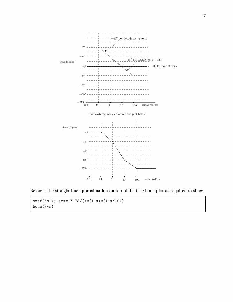
Now we draw the phase straight line approximation. Phase goes down by −450 for each pole,starting one decade before the corner frequency, and ending one decade after the cornerfrequency. This is only for the approximation factors in the form 1

1+ 𝑠𝜏. For the exact pole 1

𝑠 , it

starts at −900 and remains over the whole frequency range. For 𝜏1 = 1 rad/sec, we start from0.1 up to 10 rad/sec. For 𝜏1 = 10 rad/sec, we start from 1 rad/sec up to 100 rad/sec. Using thisinformation, below is sketch of the phase straight line approximation.

7

0.01 0.1 1 10 100

−2250

−1800

−1350

−900

phase (degree)

log(ω) rad/sec−2700

−450

00

−450 per decade for τ1 term

−450 per decade for τ2 term

−900 for pole at zero

0.01 0.1 1 10 100

−2250

−1800

−1350

−900

phase (degree)

log(ω) rad/sec

−2700

Sum each segment, we obtain the plot below

Below is the straight line approximation on top of the true bode plot as required to show.

s=tf('s'); sys=17.78/(s*(1+s)*(1+s/10))bode(sys)

8

Since the open loop is stable as it has poles at {0, −1, −0.1}, then the closed loop will be stableif there is zero net clock wise encirclement around −1. This translates to having positivephase margin when magnitude of �𝐺 �𝑗𝜔𝑔𝑐�� is unity and positive gain margin with phase is−1800.

To find the gain margin and the phase margins, we first plot our approximation of the systemfound above: 𝐺 (𝑠) = 17.78

𝑠(1+𝑠)�1+ 𝑠10 �

using the bode command. Here it is, showing on it the 𝜔𝑝𝑐

frequency (where phase is −1800) and the corresponding �𝐺 �𝑗𝜔𝑝𝑐�� in dB found, which wewill use to find the gain margin from

9

Mag

nitu

de (

dB)

-100

-50

0

50

10-1 100 101 102

Pha

se (

deg)

-270

-180

-90

HW8, problem 1, approximation of the system

Frequency (rad/s)

System: sysFrequency (rad/s): 3.2Phase (deg): -180

System: sysFrequency (rad/s): 3.19Magnitude (dB): 4

We see that at −1800, the frequency is 3.2 rad/sec. This is called 𝜔𝑝𝑐. Going back to themagnitude plot, we see that at 𝜔𝑝𝑐 then �𝐺 �𝑗𝜔𝑝𝑐��

𝑑𝐵= 4 dB. This means the gain margin

𝐺𝑀𝑑𝐵 is

𝐺𝑀𝑑𝐵 = −4 dB

Notice that 𝐺𝑀𝑑𝐵 is negative of �𝐺 �𝑗𝜔𝑝𝑐��𝑑𝐵. The reason is due to the definition of 𝐺𝑀𝑑𝐵,

which is

𝐺𝑀𝑑𝐵 = 20 log101

�𝐺 �𝑗𝜔𝑝𝑐��

But �𝐺 �𝑗𝜔𝑝𝑐�� = 10�𝐺�𝑗𝜔𝑝𝑐��𝑑𝐵

20 . Substituting this in the above gives

10

𝐺𝑀𝑑𝐵 = 20 log101

10�𝐺�𝑗𝜔𝑝𝑐��𝑑𝐵

20

= −20 log10 10�𝐺�𝑗𝜔𝑝𝑐��𝑑𝐵

20

= − �𝐺 �𝑗𝜔𝑝𝑐��𝑑𝐵

log10 10

= − �𝐺 �𝑗𝜔𝑝𝑐��𝑑𝐵

Therefore, 𝐺𝑀𝑑𝑏 is the negative of �𝐺 �𝑗𝜔𝑝𝑐��𝑑𝑏as read from bode plot. Since 𝐺𝑀𝑑𝐵 < 0 then

closed loop is not stable . To find the phase margin. we find the frequency 𝜔𝑔𝑚 which is

where magnitude plot is at 0 dB. We see that the frequency is 𝜔𝑔𝑚 = 4 rad/sec as shown inthe plot below.

Mag

nitu

de (

dB)

-100

-50

0

50

10-1 100 101 102

Pha

se (

deg)

-270

-180

-90

HW8, problem 1, approximation of the system

Frequency (rad/s)

System: sysFrequency (rad/s): 3.98Phase (deg): -188

System: sysFrequency (rad/s): 4.01Magnitude (dB): -0.0374

At 𝜔𝑔𝑚, the phase is −1880. Subtracting 1800 from this phase gives −70. Hence

11

phase margin = −70

Phase margin must be positive for stable closed loop stable. The closed loop is not stable.

Note that both the phase margin and the gain margin must be positive for stable closedloop system.

12

0.2 Problem 2

I .




r,t -\ - (r + 5)(r + 3)t i f a l F- \ - '

s ( r+ l ) ( r z * r+4 ) '




G ' ( s ) - ' 2 5 ( l + 5 s )(sr * 49.277s2 *25.172s + 2.526)





Gr(c)

SOLUTION:

The open loop

𝐺 (𝑠) =(𝑠 + 5) (𝑠 + 3)

𝑠 (𝑠 + 1) �𝑠2 + 𝑠 + 4�

has poles at 𝑠 = 0, 𝑠 = −1 and 𝑠 = −12 ±

√32 𝑗, therefore it is stable. So we expect the closed

loop to be stable only if the Nyquist plot has a net of zero clockwise encirclement around −1.When looking at the bode plot, the rules are these. The closed loop is stable, if both theseconditions are met:

1. The gain margin 𝐺𝑀𝑑𝑏 is positive. Or in other words, if �𝐺 �𝑗𝜔𝑔𝑐��𝑑𝑏is negative as read

from the bode plot.

2. The phase margin is positive.

0.2.1 Part(a)

Here is Nyquist plot

s=tf('s');sys=(s+5)*(s+3)/(s*(s+1)*(s^2+s+4));nyquist1(sys)

13

Real Axis-5 0 5 10 15 20 25 30 35

Imag

Axi

s

-40

-30

-20

-10

0

10

20

30

40Nyquist plot, problem 2, HW8

It shows there is one encirclement around −1. We can zoom in to make sure:

Real Axis-3 -2 -1 0 1 2 3

Imag

Axi

s

-8

-6

-4

-2

0

2

4

6

8

10

Nyquist plot, problem 2, HW8

The above shows that the closed loop is not stable. We will now look at Bode plot. Here isthe result, where I showed the gain and phase margins on the generated Matlab plot. Thisshows that the gain margin is negative, hence not stable, and it also shows that the phasemargin is negative, also indicating it is not stable.

14

We can also ask Matlab to give us the margins and the corresponding break frequencies.Matlab was correct and found that the closed system is also not stable:

>> [gm,pm,gwc,pwc]=margin(sys)Warning: The closed-loop system is unstable.> In ctrlMsgUtils.warning (line 25)In DynamicSystem/margin (line 65)gm =0.4254pm =-42.9450gwc =1.9239pwc =2.4785

Notice that Matlab gives the gain margin 𝐺𝑀 in linear value. We see it says 𝐺𝑀 = 0.4254above, which is −7.42 dB. Since it is negative, then closed loop is not stable.

15

0.2.2 Part(b)

We can display the cross over frequencies using Matlab either by using the margin commandor using the GUI by using the mouse as shown below. First we find the frequency where thephase is −1800, this is called 𝜔𝑝𝑐. We see it is 1.93 rad/sec. Then using the mouse, we locatethis frequency on the magnitude plot and read |𝐺(𝑗𝜔)| in dB. We see that |𝐺(𝑗𝜔)| in dB ispositive, hence 𝐺𝑀 is negative, and closed loop is not stable.

Find frequency at -180 phase

Use it to locate magnitude here.

To determine the stability using phase margin, we do the reverse. We locate the frequencywhere the magnitude is zero dB using the mouse. This is called 𝜔𝑔𝑚. We see it is at 2.48rad/sec. Then on the phase plot, we locate the phase at this frequency using the mouse. Wesee it is −2280 . Adding −1800 gives −480. Since this is negative, then the close loop is notstable.

16

Find frequency where magnitude is 0 db

Locate phase at this frequency in order to find phase margin

Using Nyquist to determine stability, we plot Nyquist. Then make a unit circle around theorigin to locate the gain and phase margin, as illustrated below

<

=

1Gm

Pm

−1

Locating gain and phase margin on Nyquist plot

Plotting the Nyquist plot using Matlab, and zooming in, and making a unit circle (Circlewas added by hand on top of the Matlab Nyquist plot), one can measure the gain and phasemargin as below

17

GM= 1/(2.34) = 0.42Phase margin = -42 degree

(angle between real line and intersection with circle)

18

0.3 Problem 3

I .




r,t -\ - (r + 5)(r + 3)t i f a l F- \ - '

s ( r+ l ) ( r z * r+4 ) '




G ' ( s ) - ' 2 5 ( l + 5 s )(sr * 49.277s2 *25.172s + 2.526)





Gr(c)

SOLUTION:

0.3.1 Part (a)

The open loop transfer function is

𝐺 (𝑠) =25 (1 + 5𝑠)

𝑠3 + 42.277𝑠2 + 25.772𝑠 + 2.526 �1 − 𝑇𝑠

1 + 0.5𝑇𝑠� �1

𝑀𝑠 + 𝐷� �1𝐾�

We start with 𝑇 = 1,𝑀 = 10,𝐷 = 1, 𝐾 = 1.

𝐺 (𝑠) =25 (1 + 5𝑠)

𝑠3 + 42.277𝑠2 + 25.772𝑠 + 2.526 �1 − 𝑠

1 + 0.5𝑠� �1

10𝑠 + 1�

And make a bode plot, then find the �𝐺 �𝑗𝜔𝑝𝑐�� at corresponding −1800.

19

Mag

nitu

de (

dB)

-150

-100

-50

0

50

10-2 10-1 100 101 102 103

Pha

se (

deg)

-180

0

180

360

HW8, problem 3

Frequency (rad/s)

System: sysFrequency (rad/s): 0.637Phase (deg): 180

System: sysFrequency (rad/s): 0.636Magnitude (dB): -3.79

But the phase do not cross −1800. This indicates an infinite gain margin. Similarly we findthat the phase margin is infinite. Hence we conclude that we can make 𝐾 as close to zero(since it is in denominator) as we want, while keeping the system stable and can make it aslarge as we want. Note that we are assuming that gain itself can only be positive here.

0.3.2 Part (b)

Both the gain and the phase margin are infinite. There is no corresponding crossoverfrequencies.

20

0.4 Problem 4

t :

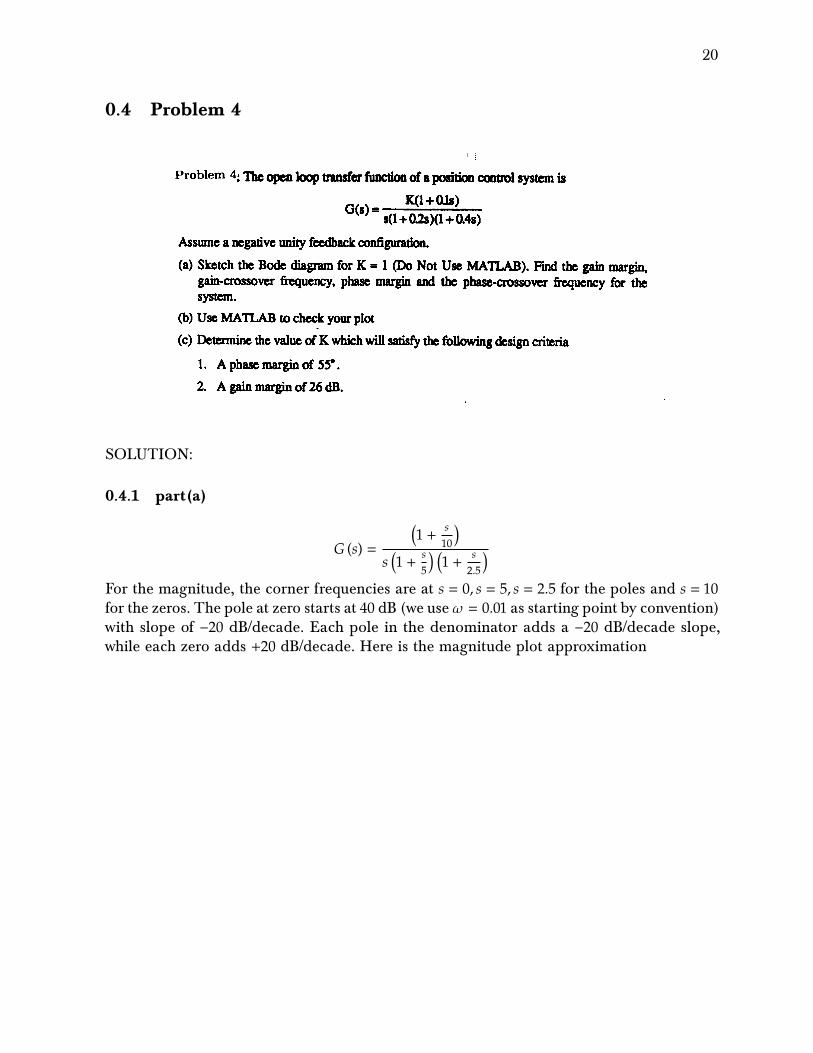
Problem 4: Thc opcn bop tnndcr ftnctim of r podtirur omuol sysrm is

G(s)-ffiAssrure a rcguive unity ftcdbackconfiguntion.

(a) Skcrch thc Bodc diagram for K = I (Do Not Usc MATLAB). Fird rhc gsin nargiagain-crossover frcquerrcn plusc margin ard thc phasc-crossorrcr @ucncy for thcsystcm.

(b) Usc MATLAB ocbcctyourplot

(c) Detcrmine the valuc of K which will satisfy thc following design criaria

l. Aphascmarginof55".

2. A gain margn of 2,6 dB.

SOLUTION:

0.4.1 part(a)

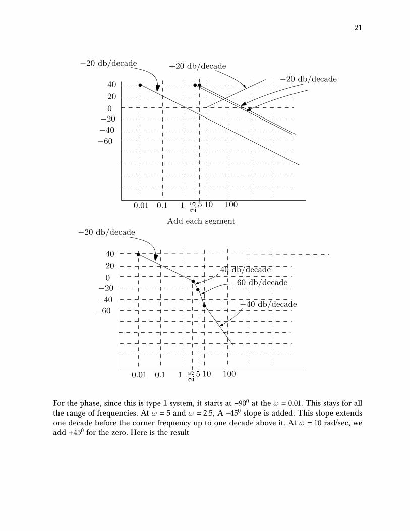
𝐺 (𝑠) =�1 + 𝑠

10�

𝑠 �1 + 𝑠5� �1 + 𝑠

2.5�

For the magnitude, the corner frequencies are at 𝑠 = 0, 𝑠 = 5, 𝑠 = 2.5 for the poles and 𝑠 = 10for the zeros. The pole at zero starts at 40 dB (we use 𝜔 = 0.01 as starting point by convention)with slope of −20 dB/decade. Each pole in the denominator adds a −20 dB/decade slope,while each zero adds +20 dB/decade. Here is the magnitude plot approximation

21

40

20

0−20

−40

−60

0.01 0.1 1 10 100

2.5 5

−20 db/decade

+20 db/decade−20 db/decade

40

20

0−20

−40

−60

0.01 0.1 1 10 100

2.5 5

−20 db/decade

Add each segment

−40 db/decade

−60 db/decade

−40 db/decade

For the phase, since this is type 1 system, it starts at −900 at the 𝜔 = 0.01. This stays for allthe range of frequencies. At 𝜔 = 5 and 𝜔 = 2.5, A −450 slope is added. This slope extendsone decade before the corner frequency up to one decade above it. At 𝜔 = 10 rad/sec, weadd +450 for the zero. Here is the result

22

−900

−1350

−1800

−2250

−2700

0.01 0.1 1 10 100

2.5 5

−450 per decade for 2.5

−450 per decade for 5

+450 per decade for zero at 10


Add all segments

0.01 0.1 1

2.5 5


Add all segments

−900

−1350

−1800

−2250

−2700

0.25

25

10010

50

0.5

Now to answer the part about the gain and phase margins. For this, we show both �𝐺 �𝑗𝜔��and phase plot that we sketched above in one diagram and mark on them the gain andphase related quantities. This is the result.

23

In next part, we use Matlab to get accurate margin values, which shows that gain marginis 30 dB and phase margin is 640. The gain cross over frequency is 7 rad/sec and the phasecross over frequency is 0.92 rad/sec. The closed loop is stable.

0.4.2 Part(b)

Using Matlab

24

clears=tf('s');sys=tf( (1+s/10)/(s*(1+s/5)*(1+s/2.5)));bode(sys);grid[gm,pm,gcw,pcw]=margin(sys)gm =30.0007pm =64.4735gcw =7.0711pcw =0.9260

Mag

nitu

de (

dB)

-100

-50

0

50

10-1 100 101 102

Pha

se (

deg)

-225

-180

-135

-90

HW 8, problem 4, part(b)

Frequency (rad/s)

0.4.3 Part(c)

Part(1)

For phase margin of 550 we want the phase at −1250 to correspond to 0 dB in the magnitudeplot. At phase −1250 the frequency is 1.3 rad/sec from the plot. At this frequency the magni-tude is −3.55 dB and not zero dB. Hence positive gain margin of 3.55 dB. We want to shift

25

this up to 0 dB. So we need to solve for additional gain from

20 log10 𝐾 = 3.55

𝐾 = 10� 3.5520 �

= 1.5

Hence

𝐾 = 1.5

To verify, here is the Matlab margin command, which shows the phase margin is indeednow 550 when using 𝐾 = 1.5

clears=tf('s');K=1.5;sys=tf( K* (1+s/10)/(s*(1+s/5)*(1+s/2.5)));bode(sys);grid[gm,pm,gcw,pcw]=margin(sys)gm =20.0005pm =55.3798gcw =7.0711pcw =1.2991

Part(2)

At −1800 in the phase plot, we want the corresponding gain margin to be 26 dB whichmeans we want �𝐺 �𝑗𝜔𝑔𝑐�� = −26 dB. Currently, we see that at −1800, the frequency is 7.1. Themagnitude is −30 dB at this frequency. We want magnitude to be −26 dB instead. Hence we

want to shift up by 4 dB the magnitude plot, or 𝐾 = 10� 420 � = 1.585

𝐾 = 1.585

To verify, here is the Matlab margin command, which shows the gain margin is close to 26dB now using 𝐾 = 1.585. (Matlab gives 𝑔𝑚 = 18.92 which is 25.54 dB)

26

clears=tf('s');K=1.585;sys=tf( K* (1+s/10)/(s*(1+s/5)*(1+s/2.5)));[gm,pm,gcw,pcw]=margin(sys)gm =18.9279pm =54.0559gcw =7.0711pcw =1.3568>> 20*log10(gm)25.5420

hw8 ece 332 feedback control · 2019-11-28 · 3 0.1 problem 1 i. - ece 332 homework f $ derivc a...

Documents