human resource planning models for … · temps, son application semble ^etre peu adapt ee a des...
TRANSCRIPT
HUMAN RESOURCE PLANNING MODELS FOR HOME HEALTH CARE
SERVICES: ASSIGNMENT AND ROUTING PROBLEMS
by
SEMIH YALCINDAG
Submitted in partial fulfillment of the requirements for the degree of
Doctor of Philosophy under a Cotutelle arrangement with
Ecole Centrale Paris and Politecnico di Milano
July 2014

c©Semih Yalcındag 2014
All Rights Reserved

To my parents

Acknowledgments
It is a pleasure to thank the people who made this thesis possible. I would like to express
my gratitude to my supervisors, Evren Sahin and Andrea Matta for their guidance, advice and
support. I would also like to thank George Shanthikumar, Paola Cappanera and Maria Grazia
Scutella for their collaboration and friendly attitude.
I also thank Jean-Charles Billaut and Nadine Meskens for their interest in this thesis for
accepting to be the reporters. My gratitude also goes to Maria Di Mascolo who did me the
honor of being the president of my thesis committee.
I am very thankful to all the members of Industrial Engineering Laboratory of Ecole Centrale
Paris and Mechanical Engineering Department of Politecnico di Milano for their warm welcome
and friendship. I am also very grateful to my friends from Turkey for their great support and
making me feel at home all the period that I spent abroad.
Finally, I would never have been able to overcome all the difficulties without unconditional
support, encouragement and love of my parents. This work is dedicated to them.
Abstract
The care givers’ assignment and routing problems are relevant issues for Home Health Care
(HHC) service providers. The first problem consists of deciding which care givers will provide
services to which patients, whereas the second aims at determining the visiting sequences of
care givers. From a modelling perspective, these problems can be solved with either a two-
stage approach or a simultaneous approach. Although the currently most known simultaneous
approach yields more accurate results by solving the assignment and routing problems at the same
time, its resolution remains computationally difficult and not viable for large scale applications.
In this thesis, we focus on the two-stage approach that sequentially solves an assignment and
a routing problem in order to compare its performances to those of the simultaneous approach.
Hence, several variants of mathematical models are developed by taking into account: (1) the
skill compatibilities between patients and operators; (2) single or multiple planning periods;
(3) imposed or released operator capacity restrictions. An important point regarding the two
stage approach concerns the estimation of care givers’ travel times that are required to solve
the assignment problem. For this purpose, we propose an empirical data-driven method that
is based on the Kernel Regression technique to estimate travel times. Such a method uses care
givers’ historical travel times that integrate several realistic factors such as cared patients’ clinical
conditions and locations or care givers’ personal preferences to estimate the time necessary for
visiting a set of patients located in the HHC service area.
Numerical studies based on realistic problem instances are used to analyze the performances
of the proposed data-driven travel time estimation method and the two-stage approach. Results
obtained show that both the newly developed travel time estimation method and the two-stage
models are promising approaches for the HHC human resource planning process.
Keywords: Home health care; human resource planning; assignment; routing; skill manage-
ment; travel time estimation; kernel regression

Resume
L’affectation des patients aux soignants et le sequencement des visites a effectuer par les
soignants sont deux problematiques interessantes observees dans les etablissements de soins
decentralises tels que les etablissements d’HAD (Hospitalisation a Domicile), de SSIAD (Soins et
services infirmiers a Domicile) ou de MAD (Maintien a Domicile). Le premier probleme consiste
en effet a decider quels soignants fourniront quels services (visites) a quels patients, tandis que
le second vise a determiner la sequence de visites de chaque soignant. Du point de vue de la
modelisation, ces deux problemes peuvent etre resolus par une approche sequentielle qui com-
prend deux etapes ou une approche simultanee. Bien que les resultats de l’approche simultanee
soient plus precis en raison de la resolution des problemes d’affectation et de routage en meme
temps, son application semble etre peu adaptee a des situations reelles, souvent de grande echelle.
Dans cette these, nous nous concentrons sur l’approche en deux etapes qui considere successive-
ment le probleme d’affectation (assignment) et de sequencement (routing) afin de comparer ses
performances a celles obtenues par l’approche simultanee. Ainsi, plusieurs variantes de modeles
mathematiques sont developpes en tenant compte de : (1) la compatibilite de competences entre
les patients et les operateurs, (2) periodes de planification uniques ou multiples, (3) contraintes
au niveau des capacites disponibles des soignants.Le verrou scientifique au niveau de l’approche
en deux etapes concerne essentiellement l’estimation de la duree des deplacements des soignants,
estimations qui sont necessaires pour resoudre le probleme d’affectation. A cette fin, nous pro-
posons une methode utilisant des donnees empiriques basee sur la technique de regression de
Kernel (Kernel Regression Technique) permettant d’estimer les durees de deplacement. Cette
methode utilise des donnees historiques sur les durees de deplacement qui integrent plusieurs
facteurs realistes concernant les conditions cliniques des patients et les conditions geographiques,
ou encore les preferences personnelles des soignants afin d’estimer la duree necessaire pour visiter
un ensemble de patients situes dans la zone de service donnee. Des etudes numeriques basees sur
des donnees reelles en provenance d’un etablissement d’HAD Italien sont realisees pour analy-
ser les performances de la methode d’estimation proposee. Les resultats obtenus montrent que
cette nouvelle methode d’estimation ainsi que l’approche en deux etapes sont des approches
prometteuses pour traiter des problematiques de planification de ressources humaines dans les
etablissements d’ HAD, SSIAD ou MAD.
Mots-cles : Hospitalisation a domicile ; planification de ressources humaines ; affectation ;
routage ; gestion des competences ; estimation durees de deplacement ; regression de kernel
Table of Contents
Acknowledgments iv
Abstract v
Resume vi
GENERAL INTRODUCTION 1Contributions . . . . . . . . . . . . . . . . . . . . . . . . . . . . . . . . . . . . . . . . . 3Outline . . . . . . . . . . . . . . . . . . . . . . . . . . . . . . . . . . . . . . . . . . . . 5
1 HUMAN RESOURCE PLANNING FOR HOME HEALTH CARE SYSTEM 81.1 INTRODUCTION . . . . . . . . . . . . . . . . . . . . . . . . . . . . . . . . . . . 81.2 HOME HEALTH CARE SYSTEM IN FRANCE AND ITALY . . . . . . . . . . 101.3 DECISION MAKING PROCESS ON THE HUMAN RESOURCE PLANNING 111.4 FUNDAMENTAL ELEMENTS OF THE ASSIGNMENT AND ROUTING PROB-
LEMS . . . . . . . . . . . . . . . . . . . . . . . . . . . . . . . . . . . . . . . . . . 12
2 ASSIGNMENT AND ROUTING PROBLEMS 252.1 INTRODUCTION . . . . . . . . . . . . . . . . . . . . . . . . . . . . . . . . . . . 252.2 ASSUMPTIONS FOR THE ASSIGNMENT AND ROUTING PROBLEMS . . . 27
I THE SIMULTANEOUS APPROACH 33I.1 INTRODUCTION . . . . . . . . . . . . . . . . . . . . . . . . . . . . . . . . . . . 34I.2 LITERATURE REVIEW FOR THE SIMULTANEOUS APPROACH . . . . . . 34I.3 MATHEMATICAL MODELS . . . . . . . . . . . . . . . . . . . . . . . . . . . . . 38
II THE TWO-STAGE APPROACH 49II.1 INTRODUCTION . . . . . . . . . . . . . . . . . . . . . . . . . . . . . . . . . . . 50II.2 LITERATURE REVIEW ON THE ASSIGNMENT MODELS . . . . . . . . . . 52II.3 PROPOSED MATHEMATICAL MODELS FOR THE ASSIGNMENT PROBLEM 54II.4 MATHEMATICAL MODELS FOR THE ROUTING PROBLEM . . . . . . . . 602.3 CONCLUSION . . . . . . . . . . . . . . . . . . . . . . . . . . . . . . . . . . . . 63
3 TRAVEL TIME ESTIMATION METHODS 653.1 INTRODUCTION . . . . . . . . . . . . . . . . . . . . . . . . . . . . . . . . . . . 653.2 OPERATOR INDEPENDENT ESTIMATION TECHNIQUE . . . . . . . . . . . 65
vii
3.3 OPERATOR SPECIFIC ESTIMATION TECHNIQUE . . . . . . . . . . . . . . 663.4 CONCLUSION . . . . . . . . . . . . . . . . . . . . . . . . . . . . . . . . . . . . . 73
4 SOLUTION APPROACHES 764.1 INTRODUCTION . . . . . . . . . . . . . . . . . . . . . . . . . . . . . . . . . . . 764.2 GENETIC ALGORITHMS . . . . . . . . . . . . . . . . . . . . . . . . . . . . . . 774.3 HOW TO CALL THE TRAVEL TIME FUNCTION . . . . . . . . . . . . . . . . 854.4 CONCLUSION . . . . . . . . . . . . . . . . . . . . . . . . . . . . . . . . . . . . . 85
5 COMPUTATIONAL STUDY 875.1 INTRODUCTION . . . . . . . . . . . . . . . . . . . . . . . . . . . . . . . . . . . 87
III ASSESSING THE PERFORMANCE OF TRAVEL TIME ESTIMATIONMETHODS USED IN THE TWO-STAGE PLANNING APPROACH 89
III.1 INTRODUCTION . . . . . . . . . . . . . . . . . . . . . . . . . . . . . . . . . . . 90III.2 DESIGN OF EXPERIMENTS . . . . . . . . . . . . . . . . . . . . . . . . . . . . 90III.3 EXPERIMENTAL SETTINGS . . . . . . . . . . . . . . . . . . . . . . . . . . . . 91III.4 NUMERICAL RESULTS . . . . . . . . . . . . . . . . . . . . . . . . . . . . . . . 95III.5 CONCLUSION . . . . . . . . . . . . . . . . . . . . . . . . . . . . . . . . . . . . 106
IV ASSESSING THE IMPACT OF THE SKILL MANAGEMENT 108IV.1 INTRODUCTION . . . . . . . . . . . . . . . . . . . . . . . . . . . . . . . . . . . 109IV.2 DESIGN OF EXPERIMENTS . . . . . . . . . . . . . . . . . . . . . . . . . . . . 109IV.3 EXPERIMENTAL SETTINGS . . . . . . . . . . . . . . . . . . . . . . . . . . . . 110IV.4 NUMERICAL RESULTS . . . . . . . . . . . . . . . . . . . . . . . . . . . . . . . 113IV.5 CONCLUSION . . . . . . . . . . . . . . . . . . . . . . . . . . . . . . . . . . . . 119
6 CONCLUSION AND PERSPECTIVES 1216.1 CONCLUSION . . . . . . . . . . . . . . . . . . . . . . . . . . . . . . . . . . . . 121
Bibliography 123
viii

List of Figures
1 The structure of the Manuscript . . . . . . . . . . . . . . . . . . . . . . . . . . . 5
1.1 Old vs Young Population Change between 2002 and 2012 for France and Itlay . . 91.2 Expected Old Person Dependency Ratio in France, Italy and Europe . . . . . . . 91.3 Alternatives for the Decision Making Process on the Human Resource Planning . 131.4 Human Resource Planning Elements . . . . . . . . . . . . . . . . . . . . . . . . . 141.5 Human Resource Planning Horizon . . . . . . . . . . . . . . . . . . . . . . . . . . 171.6 Operator Availability . . . . . . . . . . . . . . . . . . . . . . . . . . . . . . . . . . 19
2.1 Two-Stage Approach vs. Simultaneous Approach . . . . . . . . . . . . . . . . . . 28II.1 Alternative Models for the Two-Stage Approach . . . . . . . . . . . . . . . . . . 51
3.1 Optimal vs Realized (executed) Operator Tour . . . . . . . . . . . . . . . . . . . 743.2 Procedure for Implementing Kernel Technique . . . . . . . . . . . . . . . . . . . . 75
4.1 Chromosome representation for simultaneous approach with 3 operators, 10 pa-tients and 4 patterns . . . . . . . . . . . . . . . . . . . . . . . . . . . . . . . . . . 79
4.2 Chromosome representation after flipping the genes between 3th and 8th genes . 804.3 Chromosome representation for the assignment problem with KR approach . . . 824.4 Chromosome representation for TSP with 10 patients . . . . . . . . . . . . . . . 84
III.1 Example for the map of cities and patient locations . . . . . . . . . . . . . . . . . 92III.2 The trade-off between the workload balancing and the total travel time minimiza-
tion for the assignment phase of the two-stage model . . . . . . . . . . . . . . . . 101III.3 Results with Instance Group B with m=100 for Model III, IV and V . . . . . . . 104III.4 Sensitivity Analysis with Instance Group B for m=100 and m=1000 . . . . . . . 105III.5 The Trade-Off Anaylsis for the Assignment Phase Of the Two-Stage Model with
the KR and OSAV methods with m=100 . . . . . . . . . . . . . . . . . . . . . . 107III.6 Sensitivity Analysis on the Iteration Number of the GA with Instance B.1.1 and
m=100 . . . . . . . . . . . . . . . . . . . . . . . . . . . . . . . . . . . . . . . . . . 107IV.1 Comparison Between the MinMax and MinCost Objectives with Hierarchical Skills 116IV.2 Trade-off Analysis for MinMax and MinCost Objectives with Hierarchical Skills
with Medium-Sized Instances . . . . . . . . . . . . . . . . . . . . . . . . . . . . . 117IV.3 Trade-off Analysis for MinMax and MinCost Objectives with Hierarchical Skills
with Large-Sized Instances . . . . . . . . . . . . . . . . . . . . . . . . . . . . . . . 119
ix
List of Tables
1.1 Assignment and Routing Decision Attributes in HHC Services . . . . . . . . . . . 24
I.1 Classification of Existing Models Related to the Simultaneous Approach in HHCservices . . . . . . . . . . . . . . . . . . . . . . . . . . . . . . . . . . . . . . . . . 39
II.1 Classification of Existing Models Related to the First Stage of the Two-StageApproach in HHC services . . . . . . . . . . . . . . . . . . . . . . . . . . . . . . . 53
3.1 Error between the estimated and optimal travel times (as average over 100 samples) 73
4.1 Solution Methods for Different Models . . . . . . . . . . . . . . . . . . . . . . . . 774.2 Performance Analysis of the GA implemented for the simultaneous approach . . 824.3 Performance Analysis of the GA implemented for the routing problem of the two-
stage approach . . . . . . . . . . . . . . . . . . . . . . . . . . . . . . . . . . . . . 85
5.1 Summary for the Experimentations . . . . . . . . . . . . . . . . . . . . . . . . . . 87III.1 Location and probabilities of cities . . . . . . . . . . . . . . . . . . . . . . . . . . 92III.2 Parameter values used for Group B experiments . . . . . . . . . . . . . . . . . . 94III.3 Results for Group A.1, γ = 1/100, m=100 . . . . . . . . . . . . . . . . . . . . . . 97III.4 Results with Group A.2, γ = 1/750, m=100 . . . . . . . . . . . . . . . . . . . . . 97III.5 Model I results for Group A.1 and γ = 1/100 with different travel time estimators 98III.6 Model I results for Group A.2 and γ = 1/750 with different travel time estimators 98III.7 Results with 56 patients and γ = 1/100 with increasing the number of history
from 100 to 1000 . . . . . . . . . . . . . . . . . . . . . . . . . . . . . . . . . . . . 99III.8 Results with 150 patients and γ = 1/750 with increasing the number of history
from 100 to 1000 . . . . . . . . . . . . . . . . . . . . . . . . . . . . . . . . . . . . 99III.9 Results for Instance B.1.1 with different γ values and m=100 for Models III, IV
and V . . . . . . . . . . . . . . . . . . . . . . . . . . . . . . . . . . . . . . . . . . 101III.10Results for Instance Group B with m=100 for Models III and V . . . . . . . . . 102III.11Results for Instance Group B with m=100 for Model IV and V . . . . . . . . . . 103IV.1 Instance parameters for the experiment Group C . . . . . . . . . . . . . . . . . . 112IV.2 Results for Hierarchical Skills with Instance Group C.1 and Balancing Objective 115IV.3 Results for Hierarchical Skills with Instance Group C.1 and Cost Minimization
Objective . . . . . . . . . . . . . . . . . . . . . . . . . . . . . . . . . . . . . . . . 115IV.4 Results for Hierarchical Skills with Instance Group C.2, Group C.3 and Balancing
Objective . . . . . . . . . . . . . . . . . . . . . . . . . . . . . . . . . . . . . . . . 118IV.5 Results for Hierarchical Skills with Instance Group C.2, Group C.3 and Cost
Minimization Objective . . . . . . . . . . . . . . . . . . . . . . . . . . . . . . . . 118
x
GENERAL INTRODUCTION
With the ever increasing costs of operations, the service industry is faced with the tough challenge
of offering better service quality while keeping costs as low as possible. This issue is even more
important for mobile services that involve the traveling of service operators among customer sites
and eventually, the realization of on-site activities. Indeed, home delivery, appliance (elevator,
technical equipment, etc.) installation and repair services are typical examples of such services
that include the transportation of goods and personnel (competencies) spending some time at
customers’ places. Hence, with the increase in energy costs and various constraints coming from
customers or operators (e.g. different service offerings that require different skills, customer time
windows or service preferences, lunch break constraints, etc.), to be able to tackle the human
resource planning process for service operations becomes even more challenging.
Home Health Care (HHC) is an example of such mobile services that has known a fast growth
recently in the health care sector, representing an alternative to the conventional hospitalization
in developed countries [39]. As such, HHC providers deliver medical, paramedical and social
services to patients in their homes. The development of the HHC concept can be attributed
to demographic changes related to population aging, social changes in families, more people
having chronic diseases, improved medical technologies, new drugs and governmental pressures to
contain health care costs ( [2,19]). Since many resources are involved in the HHC service delivery,
including operators (e.g., nurses, physicians, physiotherapists, social workers, psychologists, home
support workers, etc.), the human resource planning process is of particular interest and consists
of several decisions such as: resource dimensioning (see [16]), partitioning of a territory into
districts (see [9]), allocation of resources to districts (see [23]), assignment of operators to patients
(or to visits) and routing (see [7]). In this research, we focus on the last two levels of planning
that are the assignment and the routing problems. Although the importance of these short
term processes, most of HHC providers still lack of methodologies and tools to improve the
performance of these processes.
1
The assignment problem refers to the decision of which operators will take care of which
patients, whereas the routing problem specifies the sequence in which the patients are visited.
To determine each operator’s route, the assignment lists of operators and, thus, the travel times
between the assigned patients should be known. Traditionally, these two problems are solved
simultaneously by using a single model. In this manuscript, we refer to this integrated model as
the ”simultaneous approach” which, in terms of modelling, corresponds to the Vehicle Routing
Problem (VRP) that exists in the current HHC literature. An alternative approach is to solve
these two problems sequentially: first, the assignment problem is solved, and then, the assignment
results and travel times between patients serve as inputs to define the routing that each operator
will perform. In this case, the individual operator route is often obtained by solving a Traveling
Salesman Problem (TSP). This approach is often used in practice and in this manuscript, we
refer to this sequential approach model as the ”two-stage procedure”.
As will be detailed in the coming chapters, the current HHC literature mostly focuses on the
simultaneous decision of assigning patients to operators and defining their routes. Because both
decisions are made at the same time, the simultaneous approach is known as theoretically the
best alternative to solve such problems. One main drawback of this approach is that it requires
solving an NP-Hard problem. In particular, in practice, there are several features that would have
an impact on the assignment and routing decisions such as the geographical locations of patients,
the care profile of patients, the availability of the person that provides help to the operator and
the geographical aspects of the territory where the HHC provider is operating. Because of these
features, in practice, minimizing total travel time may (as in the most of the existing works in
HHC literature) not be the only criterion that is required to be achieved. However, modeling and
using these features in the simultaneous approach would not be computationally tractable since
each feature would be formulated and integrated as a new decision variable or a new constraint
in the formulation of the model. An alternative method to capture such features can be obtained
by using the available historical data which would provide information regarding the choices
made in previous tours accomplished by operators. Thus, these features can be integrated into
the models with the use of the data-driven approach which will allow to make future assignment
and routing decisions based on the operator’s past behaviors. However, it is still complicated to
incorporate the data-driven technique into the simultaneous approach modeling framework.
In the two-stage approach, since the routing optimization can be considered independently
2

and exact travel times between patients are unavailable when the assignment problem is solved,
an estimation of operator travel times is required to solve the assignment problem. Travel times
can be estimated through different approaches. In this research we first use a basic approach
based on Average Values (AV) which indicates the average traveling time to reach a patient from
all other patients. Although this approach is intuitive, more accurate travel time estimation
methods might be necessary to obtain results that would more closely approximate the results
of the simultaneous approach. Thus, we propose to use the operator specific estimates via two
different techniques. As the first one, we use an extended version of the AV technique, Operator
Specific Average Value (OSAV), where each average value is calculated only with the assigned
patients of a specific operator and repeated for each operator independently. The second operator
specific estimate is proposed with the use of the previously discussed data-driven approach which
might enable the capture the accomplished route choices and permitting travel time estimations
based on the past behaviors.
Finally, we also developed different models to be able to consider several realistic situations
where different operator and patient skills are incorporated hierarchically (simultaneously) or
independently for single (i.e. a day) and multiple planning periods (i.e. multiple days). Since in
real practice patients usually have different care requirements and operators have various qual-
ification (skills), alternative skill management ways for the skill compatibility between patients
and operators are crucial. Thus, in addition to the case where all skill levels are managed inde-
pendently, we also consider the case where over skilled operators are able to care patients with
lower skill requirements (i.e. hierarchical skill management). Such variety of models enable us
to consider as much different cases as possible that can be applicable to differently structured
health care providers from different regions and countries.
Contributions
This work has several contributions that can be described as follows:
The first one is to present the existing HHC literature that is available for the assignment
and routing problems. To do this, we first present a detailed framework in Chapter 1 which is
used to classify the important features (i.e. travel time, service time, planning period etc.) of the
assignment and routing problems based on organization, geography and patient related aspects.
We then, classify the existing works according to this framework in Chapter 2, section I.2 and
3

II.2 respectively. To our knowledge, such a recent literature review does not exist.
The second contribution is to propose a methodology to decompose the assignment and
routing problems into two stages by considering several criteria such as operators’ workload
balancing, continuity of care, multiple operator and patient skills, multiple planning periods and
travel time reduction. Details related to the models are provided in Chapter 2. The two-stage
approach provides a significant contribution to the HHC literature since it enables to take into
account more realistic situations than the currently available simultaneous approach and also
allows to tackle complex instances characterized by larger number of patients and operators.
The third contribution, which is presented in Chapter 3, is to provide alternative travel time
estimation methods for the assignment problem of the two-stage approach. Among the presented
estimation methods, data-driven technique is the most crucial one for HHC services because it
uses the travel times observed from previous periods to estimate the time for visiting a set of
patients located in specific geographical locations.
The last contribution of this thesis is to analyze the performance of the proposed two-stage
models in comparison to the simultaneous approach. To this end, several numerical experiments
are conducted in Chapter 5.
All these goals have already been or will be presented in journals or conference publications
as follows:
• The presented literature review in Chapter 2 is published in the proceedings of the 37th
Conference on Operational Research Applied to Health Services (ORAHS 2011) with the
title ”Human Resource Scheduling and Routing Problems in Home Health Care Context:
A Literature Review”.
• The two-stage approach model (presented in Chapter 2) with the average travel time esti-
mation technique ( provided in Chapter 3) is published in the proceedings of the 8th annual
IEEE International Conference on Automation Science and Engineering (CASE 2012) with
the title ” Operator Assignment and Routing Problems in Home Health Care Services”.
• A new data-driven travel time estimation method (provided in Chapter 3) for the assign-
ment problem of the two-stage approach is developed and published in the proceedings of
the 1st International Conference on Health Care Systems Engineering (HCSE 2013) with
the title ”A Two-Stage Approach for Solving Assignment and Routing Problems in Home
4
Health Care Services”.
• An extension of the work published in the proceedings of HCSE 2013 has been submitted
to European Journal of Operational Research for publication with the title ”The Assign-
ment Problem in Home Health Care: A Data-Driven Method to Estimate Travel Times of
Operators”.
• Models considering skill management alternatives that are presented in Chapter 2 for the
two-stage and simultaneous approaches are being compared in the ongoing work and will
be submitted to the Journal of Production and Operations Management.
Outline
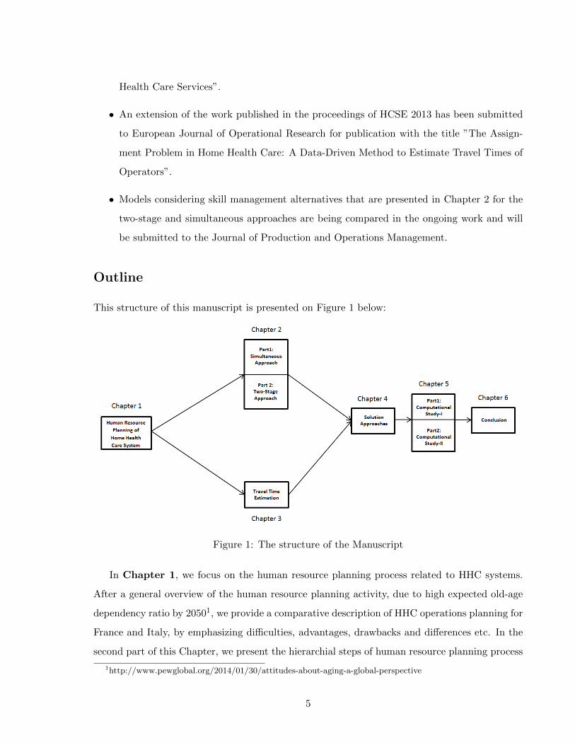
This structure of this manuscript is presented on Figure 1 below:
Figure 1: The structure of the Manuscript
In Chapter 1, we focus on the human resource planning process related to HHC systems.
After a general overview of the human resource planning activity, due to high expected old-age
dependency ratio by 20501, we provide a comparative description of HHC operations planning for
France and Italy, by emphasizing difficulties, advantages, drawbacks and differences etc. In the
second part of this Chapter, we present the hierarchial steps of human resource planning process
1http://www.pewglobal.org/2014/01/30/attitudes-about-aging-a-global-perspective
5
including the assignment and routing problems that are analyzed in further details afterwards.
As such, a framework that classifies HHC attributes related to organization, geography and the
patient is proposed to classify the existing work in the HHC literature.
Chapter 2 consists of two main parts. Part I presents the simultaneous approach where
we first provide a comprehensive literature review based on the framework presented in Chapter
1.4. Then, we present the mathematical programming models including assumptions considered
and different modeling alternatives. Part II describes the two-stage approach that we propose.
We start with the first-stage, the assignment problem, of the presented approach and then we
provide details for the second-stage where details related to the routing problem are given. For
the first-stage, we present the literature related to the stand-alone assignment problem applied to
HHC services and then we provide the existing and newly developed mathematical programming
models with the related assumptions and alternatives. Finally, the routing models that are used
to solve the second stage of the two-stage process are presented in details.
Chapter 3 focuses on the travel time estimation methods to be able to use the two-stage
process. We first explicitly present the details of the different alternative methods based on
the average value and data-driven approaches. Since data-driven approach is one of the main
focus of this thesis, the chapter ends with a convergence and accuracy analysis of this estimation
alternative.
Chapter 4 presents the solution techniques that are used throughout this research. We
present two different approaches that are adopted to solve the previously detailed mathematical
models where the first one is based on a commercial CPLEX solver and the second one is based
on a heuristic approach. Since, the choice of the solution algorithm depends on the used travel
time estimation method, implementation details for each travel time function are also provided
throughout this chapter.
In Chapter 5, several experiments are executed with the instances generated from real data
and then associated numerical analysis is presented under two main parts. The first part (see
Part III) presents the results with hierarchical skill models and the second part (see Part IV)
provide results for the independent skill models. According to the analysis based presented in
these parts, it is observed that the two-stage provides as good solutions as the simultaneous
approach does based on the objective functions. It is also seen that the presented data-driven
approach performs better than other travel time estimation methods. Thus, this makes the two-
6

stage approach with the data-driven travel time estimation technique as a promising method for
future works.
Finally in Chapter 6, conclusions, limits of this research are discussed. Some future per-
spectives are also provided.
7
Chapter 1
HUMAN RESOURCE PLANNING FOR HOME HEALTH CARE SYSTEM
1.1 INTRODUCTION
HHC services emerge as an increasingly promising alternative for providing health and social
services to patients at their homes. Many factors drive the need and demand for HHC such as
the demographic trends, changes in the epidemiological landscape of disease, the increased focus
on user-centered services, the availability of new support technologies and the pressing need to
reconfigure health systems to improve responsiveness, continuity, efficiency and equity. HHC
aims at satisfying people’s health and social needs at their home by providing appropriate and
high-quality health and social services within a balanced and affordable continuum of care.
HHC is considered and serviced differently around the countries across Europe. The differen-
tiation occurs because health services are usually regulated within the framework of a national
health system (i.e. Greece, Italy, the United Kingdom) or a national social insurance system
(i.e. Austria, France, Germany and the Netherlands), while the social welfare systems usually
administered by regional or local governments.
The proportion of older people in the general population is increasing in many European
countries and is predicted to rise further in the coming decades. In this thesis, we consider 2
European countries, France and Italy, where this case is observed for the last 10 year1 (See Figure
1.1). In particular, the ratio of care-dependent people in these counties are expected to increase
steadily even more than many other European Countries (i.e. 25 Countries) for the coming three
decades as well2 (See Figure 1.2).
1http://www.who.int/2http://epp.eurostat.ec.europa.eu/portal/page/portal/population/data/main tables
8

Figure 1.1: Old vs Young Population Change between 2002 and 2012 for France and Itlay
Figure 1.2: Expected Old Person Dependency Ratio in France, Italy and Europe
In the following part, we present the health care system of these countries to better analyze
the differences and similarities of the provided HHC service. In particular, we provide details for
2 real health care providers from France and Italy as well. Lastly, we mention and position the
human resource planning process in the HHC services.
9
1.2 HOME HEALTH CARE SYSTEM IN FRANCE AND ITALY
HHC services are organized under different structures in France and Italy. Generally, in France,
the organization is managed by social insurance and local government or by the municipality.
On the other hand, in Italy central or regional government takes care the organization issue of
the HHC services. In France, the service delivery is provided to different age categories (i.e.
child care or elderly people etc). On the contrary, in Italy although several age categories are
considered as well, the main focus is on the elderly people. One other difference in the HHC
system of these counties is the pricing condition. In France, big percent of the HHC service cost
(i.e. around %80) is supported by the health insurance and the remaining part is paid by the
patient. In Italy, HHC services are delivered free of charge and supported directly by the national
health system and by the local health units. Beside the differences, the admission conditions for
HHC services are mainly similar in both service structures. In both countries, the patient is
moved from hospital to home care with the decision of the doctor in charge. In particular, after
the decision of the doctor, family members of the patient should also agree with the transfer from
hospital to the home environment. Here below details for 2 real service providers are presented.
1. CHU Grenoble, France:
It is founded in 1969 as the first HHC provider of the province. It is dedicated to home
support for adults, pediatric patients with relatively severe disease and requiring hospital
care, and maternity patients. The service is provided in a geographical area ranging up to
about 40 km from the hospital that the operators mainly work for. They have capacity of
80 people, divided into three areas: 58 adults, 14 seats maternity and 8 pediatric patients
and these patients are served by the team consists of 48 people including doctors, nurses,
social workers, coordinator etc.
2. MOSAICO Milan, Italy:
MOSAIC is a company of SEGESTA group that provides health and social care services at
home. Since 1999 it works in partnership with local health authorities (ASL and hospitals)
in the provinces of Milan, Monza and Pavia. MOSAICO provides free service to the patients
mainly with age of 65 and over (i.e. around % 87 of the total capacity) without considering
their economic conditions. The service is provided with different category of operators
including doctors, nurses, physiotherapists, coordinator etc.
10
As it can be recognized, these providers have different management strategies where the one
from France is a part of the hospital and resources are shared between the hospital and home
services. On the other hand, the Italian provider serves as an autonomous center and receives
patients from several hospitals. Although it is also possible to see this management structure in
France as well, the reverse case is not available. In particular, although both provide service to
different age categories, the Italian provider has higher percentage of caring older patients than
the French provider. Thus, we can conclude that different countries have different considerations
and management strategies for the HHC services.
Even there are differences in the HHC systems, human resource planning process is always
in the center of attention almost in all countries. Although we can also observe differences on
the human resource planning strategies, the decision making processes is quite general. Hence,
in the following section, we present details of the general decision making process in details.
1.3 DECISION MAKING PROCESS ON THE HUMAN RESOURCE PLAN-
NING
There are several issues that should be considered in the decision making process of the human
resource planning of the HHC services, such as the resource dimensioning, partitioning of a
territory into districts, allocation of resources to districts, assignments of operators to patients
or the visits and the operator routing.
These issues can be classified as long, medium or short term decisions. Among them, parti-
tioning of a territory into districts can be considered as a long term decision whereas assignment
and routing processes of operators can be considered as medium and/or short term decisions.
Although the focus of this thesis is on resource assignment and routing processes, it is also
interesting to be aware of processes that take place before the assignment and routing processes.
Figure 1.3A presents all the procedure explicitly. The first step is the resource dimensioning issue.
Here, the number of operators are determined to meet the predetermined care demand with the
minimum cost and the adequate service quality. The second step is partitioning of a territory
into districts. This consists of grouping small geographic areas into larger clusters, which are
named as districts, according to relevant criteria where each district is under the responsibility
of a multidisciplinary team. Once districts are determined, resources are assigned to districts
and then to patients equitably. After that the successive steps are the assignment and routing
11
processes.
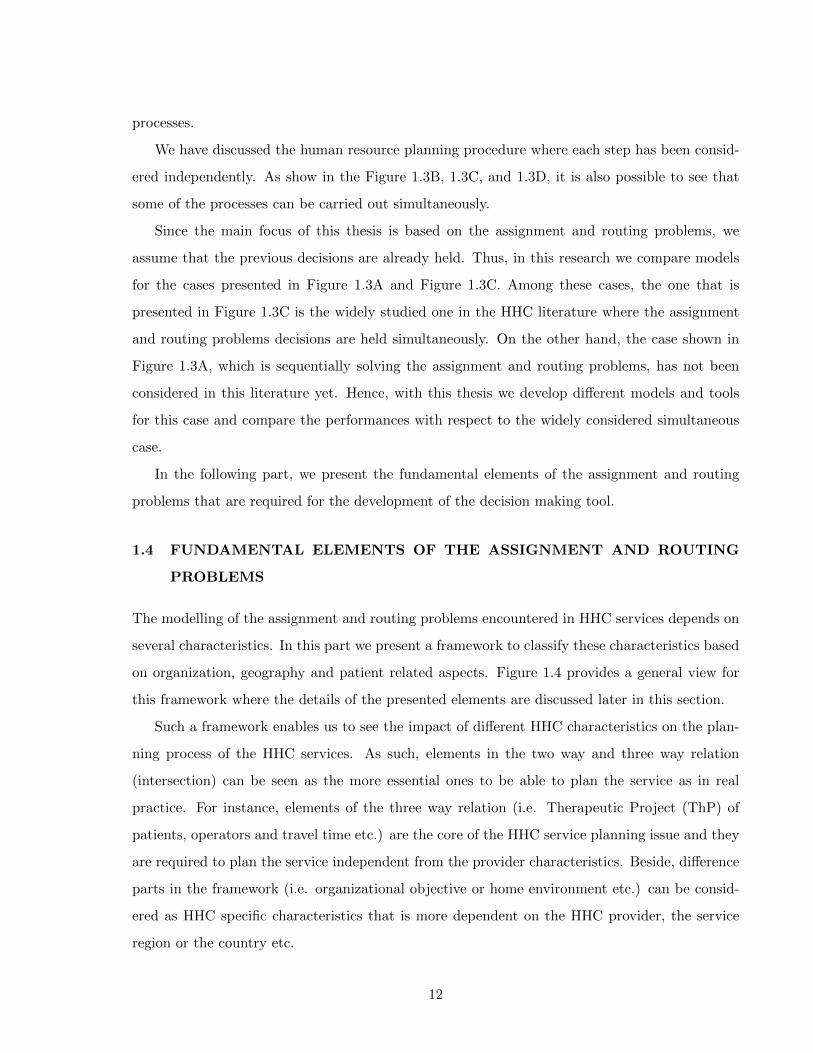
We have discussed the human resource planning procedure where each step has been consid-
ered independently. As show in the Figure 1.3B, 1.3C, and 1.3D, it is also possible to see that
some of the processes can be carried out simultaneously.
Since the main focus of this thesis is based on the assignment and routing problems, we
assume that the previous decisions are already held. Thus, in this research we compare models
for the cases presented in Figure 1.3A and Figure 1.3C. Among these cases, the one that is
presented in Figure 1.3C is the widely studied one in the HHC literature where the assignment
and routing problems decisions are held simultaneously. On the other hand, the case shown in
Figure 1.3A, which is sequentially solving the assignment and routing problems, has not been
considered in this literature yet. Hence, with this thesis we develop different models and tools
for this case and compare the performances with respect to the widely considered simultaneous
case.
In the following part, we present the fundamental elements of the assignment and routing
problems that are required for the development of the decision making tool.
1.4 FUNDAMENTAL ELEMENTS OF THE ASSIGNMENT AND ROUTING
PROBLEMS
The modelling of the assignment and routing problems encountered in HHC services depends on
several characteristics. In this part we present a framework to classify these characteristics based
on organization, geography and patient related aspects. Figure 1.4 provides a general view for
this framework where the details of the presented elements are discussed later in this section.
Such a framework enables us to see the impact of different HHC characteristics on the plan-
ning process of the HHC services. As such, elements in the two way and three way relation
(intersection) can be seen as the more essential ones to be able to plan the service as in real
practice. For instance, elements of the three way relation (i.e. Therapeutic Project (ThP) of
patients, operators and travel time etc.) are the core of the HHC service planning issue and they
are required to plan the service independent from the provider characteristics. Beside, difference
parts in the framework (i.e. organizational objective or home environment etc.) can be consid-
ered as HHC specific characteristics that is more dependent on the HHC provider, the service
region or the country etc.
12

Figure 1.3: Alternatives for the Decision Making Process on the Human Resource Planning
13
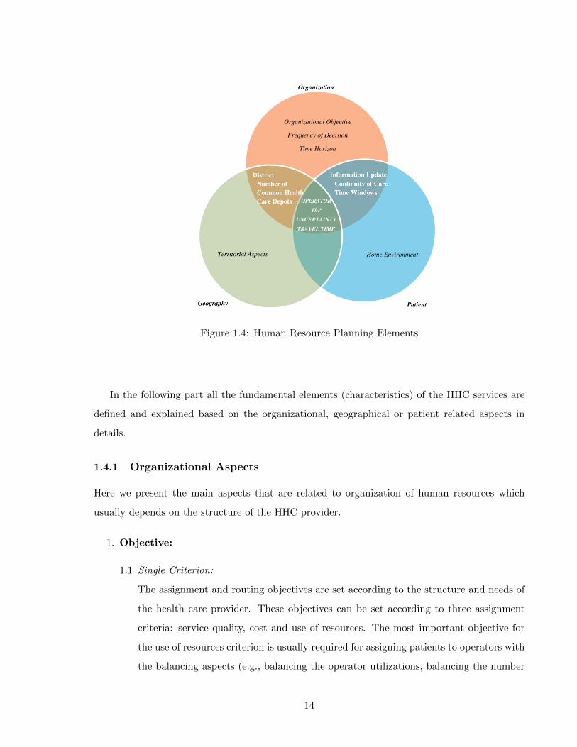
Figure 1.4: Human Resource Planning Elements
In the following part all the fundamental elements (characteristics) of the HHC services are
defined and explained based on the organizational, geographical or patient related aspects in
details.
1.4.1 Organizational Aspects
Here we present the main aspects that are related to organization of human resources which
usually depends on the structure of the HHC provider.
1. Objective:
1.1 Single Criterion:
The assignment and routing objectives are set according to the structure and needs of
the health care provider. These objectives can be set according to three assignment
criteria: service quality, cost and use of resources. The most important objective for
the use of resources criterion is usually required for assigning patients to operators with
the balancing aspects (e.g., balancing the operator utilizations, balancing the number
14
of patients per operator etc.). An objective related to the cost criterion can be required
for the both assignment and routing decisions. For the routing, it can be the reduction
of travel times traversed by all of the operators or reduction of penalty costs of visiting
other districts. For the assignment case, cost criteria can be the reduction of the cost of
hiring external operator or the reduction of overtime costs etc. Moreover, the objective
for the service quality aspect can be imposed by considering the continuity of care issue
especially for the assignment decision.
1.2 Trade-off Function:
Depending on the service structure, it is also possible to consider trade-off between the
use of resources and cost criteria (i.e., trade-off between the balancing values and total
travel times of operators) while assigning patients to operators and obtaining visiting
sequences of operators.
2. Time Horizon:
Planning horizon in HHC context is a time period, during which, health care provider will
plan the service. In the planning horizon, decision is based on three aspects: elementary
assignment and/or routing period, assignment and routing horizon and information update
interval.
2.1 Assignment and routing horizon (T):
Planning process in the HHC is based on the available information (e.g., patient de-
mand). To make decisions, planners should consider the maximum length of the avail-
able information (for how many periods the data is available). Thus, the assignment
and routing horizon is the period where the overall assignment and routing decisions
are supposed to be planned based on the length of the available information.
2.2 Information update interval (U):
The health care provider should also decide how to update the assignment plan. Infor-
mation update is usually based on the information related to patients and operators
(i.e., patient demand, operator availability, etc.). Since new patients are entering to
the system, the conditions of previously admitted patients and operator availibilies are
subject to change, the information update interval is important to respond the needs
of patients at the right time. Different alternative cases are present and can be clas-
15
sified under two main groups: decision with a fixed time frequency or decision with a
condition.
In the fixed time frequency case, independent from the specific patient or operator
information, the information can be updated at the beginning of each period (e.g., day,
week or month). Alternatively, in the decision with a condition case, information can
be updated by a given condition. This condition can be updating with the arrival of
each new patient (when a patient enters to the system, assignment process is held) or
with the arrival of certain number of new patients (group of patients).
Using one of these alternatives depends on the organizational structure of the health
care provider. Each provider may decide to use either alternative depending on their
structure. If the provider chooses to use the second alternative, they also need to decide
the condition of the decision. As indicated before, condition can be repeating decisions
for each single newly admitted patient or a batch of patients. The single patient case
can be used to increase the quality of the service. Serving patients as they arrive to
the system will help to increase their satisfaction levels because they do not wait in
the system and as soon as they enter, they are served with an operator. Decreasing
waiting times is one of the important aspects to serve with a higher quality. On the
other hand, assigning when the predetermined number of patients are obtained can
be more efficient. This case is similar to the inventory control problem. With this
alternative health care provider is also able to have more control over the capacity of
the HHC system. In addition, health care provider can assign nurses to the waiting
patients to do pre-assisting and this could be useful to avoid the quality problems due
to waiting times to obtain the predetermined number of arrivals.
2.3 Elementary assignment (A) and/or routing (R) period (P):
Previous parts provided details for the planning horizon based on the whole decision
period and the plans update interval. In addition to these information, it is also im-
portant to emphasize the elementary period where this responds the question of when
to make or repeat each assignment and routing decisions. Usually, the whole decision
period is relatively larger than this elementary decision period. This period(s) can be
considered as sub-periods of the whole decision period where the assignment and rout-
ing decisions are held. For example, HHC provider may decide to do the assignments
16
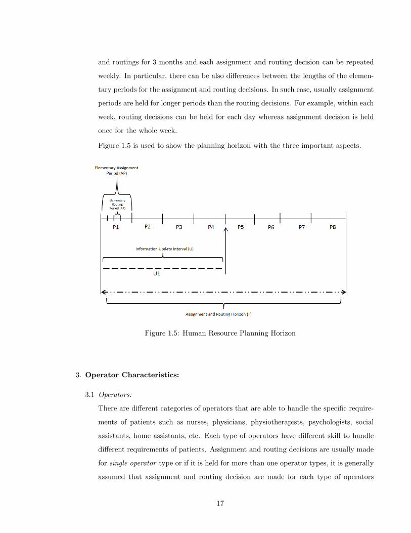
and routings for 3 months and each assignment and routing decision can be repeated
weekly. In particular, there can be also differences between the lengths of the elemen-
tary periods for the assignment and routing decisions. In such case, usually assignment
periods are held for longer periods than the routing decisions. For example, within each
week, routing decisions can be held for each day whereas assignment decision is held
once for the whole week.
Figure 1.5 is used to show the planning horizon with the three important aspects.
Figure 1.5: Human Resource Planning Horizon
3. Operator Characteristics:
3.1 Operators:
There are different categories of operators that are able to handle the specific require-
ments of patients such as nurses, physicians, physiotherapists, psychologists, social
assistants, home assistants, etc. Each type of operators have different skill to handle
different requirements of patients. Assignment and routing decisions are usually made
for single operator type or if it is held for more than one operator types, it is generally
assumed that assignment and routing decision are made for each type of operators
17

independently. In another case, if it is decided to use more than one operator type
simultaneously, this can be considered as the team assignment and routing decisions.
3.2 Operator Skills:
Operators from each type have a main skill and may also have some additional skills
to serve the different needs of the patients. The main skill of the operator is the one
that is best suited to care a particular patient from a specific category (full knowledge
of patient characteristics, etc.). With the additional skills an operator is also able to
handle patients from different categories in addition to the category of his/her main
skill.
For example, if a provider is serving for both palliative and non-palliative patients,
hierarchial skilled operators can take care of both palliative patients (main skill) and
non-palliative patients (additional skill). On the other hand, if the service is provided
to only one type of patients, operators will be called identical skilled operators. In this
case, there is not a distinction between main and additional skills.
3.3 Operator Availability:
Operator availability is the period, over a time frame, where the operator is able to
serve the patients. Operator availability is usually considered according to the working
contract and reliability. Availability is based on the contract type of the operator.
The operator can be full time, half time or external employee of the provider. Full
time employment is the general case where the health care provider is just accepting
new patients according to its available capacity. Some health care providers may want
to work in shifts (with half time employees) and instead of using an operator during
whole day, they may want to split daily workload among different operators and ask
operators work half a day (i.e., according to specific operator time windows. Although
planning working days in shifts can be more complex to organize, asking less work
during a day might be useful to increase operators motivation levels. Lastly, due to
some special care types or insufficient number of operators, the health care provider
may also need to use employees from external resources. Depending on the structure
of the health care provider, they can use one, two or all of these different contract
types to response the needs of the patients. Reliability of the operator is another
important aspect related to the availability of the operator. Reliability is the ability
18

of a operator to perform and maintain its functions in routine circumstances. Due to
personal reasons or illnesses, one or more operators may not be available during some
time periods. Thus, considering the unavailability might be crucial to make better
decisions. Other important concepts related to the contract and reliability aspects are
the utilization rates, overtime hours and efficiency of operators. Utilization rate is the
ratio between the actual workload and the operators capacity. This rate can be used
to measure the availability of the operator. In addition, it is also possible for operators
to work beyond their capacities according to the need of the HHC provider (overtime)
(i.e., soft operator time window). In such case, HHC provider usually need to pay
additional costs for each overtime hour exceeding the regular capacity of an operator.
In particular, efficiency is defined as the ratio of time that the operator is available to
the total time it is required.
Figure 1.6 is used to show the differences between operator capacity, operator avail-
ability and the overtime period.
Figure 1.6: Operator Availability
3.4 Service Time:
The service time is the duration in which the operator provides the required care service
to the patient. In real practice, since the service is provided with different operators to
different patients, the service time can be variable. There are several factors that may
cause this variability. The main factor is the operator-patient match which is based
on the Thp of the patient. For example, different operator skills require different care
durations according to the associated complexities. Similarly, if an operator has an
19
additional skill, the intervention times of using the additional skill might be longer in
comparison to his/her main skills. Thus, this results in different operation times. In
particular, in some cases where all patients have identical requirements from identical
skilled operators, service time can also be identical and fixed (i.e., 45 minutes per visit).
1.4.2 Geographical Aspects
Here are the main aspects that are related to territory where the HHC provider is providing the
service on.
1. District:
Districts are clusters where operators and patients grouped according to relevant criteria
such as territory, skill and compatibility condition of the patient. There are two main ways
of considering districts: single district or multi districts.
1.1 Single District:
The organizational structure has a important impact on the provider’s districting
scheme. The single district case is the simpler alternative that the provider does not
split the geography into smaller clusters. However, to fully exploit special skills, opera-
tors can be preferred to be controlled among multiple districts. In such case, the health
care provider is managing more than one district to serve its patients. Since there are
more than one district, the provider may decide to serve each district independently
as an autonomous decision center.
1.2 Multiple District:
Alternatively, the provider can also decide to serve districts in a integrated way. In
this way, operators are also able to serve other districts that are not their primary
one with a penalty cost. In another case, districts can also be formulated as they
are intersecting. This provides more flexibility to the provider and they can allocate
operators to more than one district without any additional cost.
2. Health Care Center:
2.1 Single Health Care Center:
20

In general, operators start and finish their daily activities in a common health care
center.
2.2 Multiple Health Care Center:
If the service area is big and not easily accessible because of territorial aspects (i.e.,
urban, non-urban area), there can be more than one common health care centers and
operators start and finish their service in one of these centers. Another alternative
location can be the houses of the operators. In such a case, operators may only need
to visit the common center on the beginning of the planning period and in the rest of
the time they can serve their patients starting from their own houses.
1.4.3 Patient Related Aspects
Here are the aspects that characterizes the main profiles of patients that are associated to the
HHC provider.
1. Patient:
1.1 Classification:
Patients are usually classified into different categories depending on the type (required
operator type and skill) and intensity (volume) of the service requested (e.g., palliative
and non palliative). Patients are also classified according to their physical presence in
the system such as currently in service or planned future arrivals. With the admission
to the system, the health care provider performs the Therapeutic Project (ThP). Once
a ThP is defined, a category, namely care profile (CP), is assigned to the patient
based on the pathology, requested operator type, required number of visits and home
environment (either the people at home eligible to do services like cleaning or not).
1.2 Demand:
Patient demand is the service requirement of each patient in the given time period.
There are different cases related to the patient demand as considering only the demand
of the single period or multiple periods. It is also possible to update the demand
information according to the condition of the patient. More detailed information was
given in the time horizon part of this section.
21
1.3 Availability:
Patient availability is usually identified by the physical presence or time window of
the patient. As described before according to ThP of the patient, a CP is assigned
to the patient and this is usually revised periodically. According to this information,
sometimes patients need to be served at hospital instead of their home. In such case, the
patient is removed from the HHC system for some periods and he/she is not anymore
available (physically not present) until the next arrival. In particular, time windows
(i.e., hard time windows) restrict the times at which a patient is available to receive a
service. Other than these time slots, patients are considered as unavailable and it is not
possible to serve them. On the other hand, the patient may also ask to be visited on the
preferred time slots due to some personal reasons. This case is commonly considered
as soft time windows and these time windows can be violated with a certain penalty.
2. Continuity of Care:
The continuity of care aspect can be grouped as full, partial or no continuity of care. The
provider use one of these groups according to the patient availability, operator availability
and also the length of assignment horizon. The full continuity of care is pursued by several
HHC providers to assign a patient to only one operator who is responsible for the care
during his/her stay in the HHC service. Since loss of information between operators is
avoided and the patient does not need to develop new relations with new operators, the
full continuity of care is considered as a crucial indicator of the service quality. The partial
continuity of care is also important where a patient requires more than one type of care. If
one of the care types is more frequent (more than fifty percent of total care required), then
a reference operator can also be assigned (like in the full continuity of care case) but some
other operators are also needed to provide other required care services. In the no continuity
of care case the provider does not need to respect the operator-patient assignments from
previous periods. Each new assignment period starts with new assignment process where all
available operators can be assigned to all patients according to their skills and requirements.
3. Uncertainty:
In real practice, it is usually not possible to know all the necessary information at the
beginning of the planning horizon such as patient demand, patient availability, operator
availability, travel time or service time. Since all these information are usually uncertain,
22
to have more realistic assignment and routing solutions considering the uncertainty of one
or more than one of these elements might be significant.
4. Travel Time:
Travel time is the duration that the operator spends on the way between each patients and
the common health care center (depot).
4.1 Real Travel Time:
If the assignment and routing decisions are held at the same time by the simultaneous
approach, real travel times (i.e. euclidian distance ) between each patient is available.
4.2 Estimated Travel Time:
The time needed to travel from one patient to the other depends on the sequence of
visits defined for each operator. In the two stage problem, the optimal visit sequence is
obtained by solving a sequencing problem based on patients assigned to a given oper-
ator. That is why, for the stand-alone assignment problem since the visiting sequence
of patients are not yet obtained (i.e. the sequencing problem is not solved), relevant
travel time estimations are necessary. This modeling aspect and different alternatives
of the travel time estimation will be discussed on following chapters.
Until now, we have identified and detailed characteristics for the assignment and routing
problems of the HHC services. Here below, Table 1.1 summarizes these characteristics in the
light of the framework that we have developed and with respect to the available HHC literature.
This table will be used in the following chapter (in Section I.2 and Section II.2) for presenting
and comparing the available literature.
Note that this is a subjective analysis where each attribute is considered in one of the three
attribute families according to our choice. Other considerations like considering operator under
patient attribute family can also be a alternative representation.
In the following chapter, we present the assumptions, literature reviews and models for the
assignment and routing problems of the HHC services.
23

1 Organization1.1 Objective
1.1.1 Single Criterion1.1.1.1 Travel Time Minimization1.1.1.2 Penalty Cost Minimization1.1.1.3 Workload Balancing
1.1.2 Trade-off Function1.2 Time Horizon
1.2.1 Single Period1.2.2 Multiple Period
1.3 Operator Characteristics1.3.1 Single Operator1.3.2 Multiple Operator1.3.3 Identically Skilled Operators1.3.4 Different Skilled Operators1.3.5 Operator Availability1.3.6 Operator Capacity1.3.7 Full Time Contract1.3.8 Half Time Contract1.3.9 External Operator1.3.10 Service Time
1.3.10.1 Identical1.3.10.2 Variable
1.3.11 Time Windows2 Geography
2.1 Number of District2.1.1 Single District2.1.2 Multiple Districts
2.2 Number of Common Health Care Center2.2.1 Single Health Care Center2.2.2 Multiple Health Care Centers
3 Patient3.1 Time Window Constraint on Visits3.2 Continuity of Care3.3 Uncertainty3.4 Travel Time
3.4.1 Real Travel Time3.4.2 Estimated Travel Time3.4.3 Travel Time is Not Explicitly Considered
Table 1.1: Assignment and Routing Decision Attributes in HHC Services
24
Chapter 2
ASSIGNMENT AND ROUTING PROBLEMS
2.1 INTRODUCTION
As presented in Section 1.4, once the patient is admitted to the HHC service, according to his/her
therapeutic project, the resource assignment and routing problems are solved to plan the visiting
activities of operators. The assignment problem decides which operator will provide care for
which patients and the operator routing problem specifies the sequence in which the patients
assigned are visited. The planner tries to provide patients with convenient service according
to their specific needs such as planning visit to the patient within appropriate time interval
according to the availability of the person who provides help to the operator. He/she also tries
to minimize operational costs in terms of distances traveled by operators such as planning the
visiting sequence of an operator according the the geographical locations of the assigned patients
(i.e. visiting the closely located patients one another). Lastly, the planner also tries to satisfy
eventual operator preferences such as avoiding the planning of specific patient visits (i.e. located
in the city center) in rush hours.
To specify each operator’s route, the assignment lists of operators as well as the travel times
between the assigned patients should be known. Most of existing work in the literature solve
these two problems simultaneously where the assignment and routing decisions are held at the
same time (i.e. VRP). Generally, this problem is formulated in a single model using data such as
required visiting frequencies of patients (i.e., number of times that the patient should be visited
in a given week), durations of patient visits, operators’ capacities, operators’ skills, and Euclidean
distances that separate patients, which are deduced from their geographical locations (given by
Euclidean distances).
Because both decisions occur at the same time, the simultaneous approach is known as
25
theoretically the best alternative to solve such problems. However, in practice, other features
than the geographical locations of patients (i.e., euclidian distances) would have an impact on
the assignment of patients and the routes that each operator would use. Examples of such
features can stem from features related to patient care requirements (i.e., their care profiles) or
the geographical aspects of the territory the HHC provider is operating. For instance, the visit
of a patient requiring a blood test would most probably be done early in the morning, although
it could be optimal to visit him/her at the end of the day if only a travel time minimization
criterion is applied. Furthermore, because of physical constraints over the territory or implicit
operator personnel preferences, some sequences of visits would never be realized in practice
(although possible theoretically). Other features such as information regarding the availability,
for a given day, of patient family members that help operator is another feature that would drive
the operator to modify the planned sequence of visits. Because of these features, in practice,
the HHC planner would assign a patient to a different operator than the one to whom she/he
would be assigned when only the geographical criterion based on average or euclidian traveling
values is used. In other words, minimizing total travel time may not be the only criterion that
is wanted to be achieved.
Modeling and integrating such features to the simultaneous approach would not be compu-
tationally tractable since one would have to formulate each feature as a new decision variable
or a new constraint and integrate it to the formulation of the model. Thus, we propose a new
approach where assignment and routing problems are solved sequentially with the two-stage pro-
cedure: first, the assignment problem is solved, and then, assignment results serve as inputs to
define the route that each operator performs. In this case, the individual operator route is often
obtained by solving a Traveling Salesman Problem (TSP) model.
In the first stage, the assignment problem needs to be solved to obtain the assignment list of
each operator based on patients’ care requirements (i.e., required visiting frequency, service time
and operator skill) and operator availabilities. Because the routing optimization is considered
independently and exact travel times between patients are unavailable when the assignment
problem is solved, an estimation of the travel time necessary to reach each patient is also required
to solve the assignment. To this end, in Chapter 3 we present different travel estimation methods
in details. Even if the two-stage approach is an approximation of the simultaneous approach,
it has several advantages that makes it worth to use. First, it enables to take into account
26
the impact of several factors and operator behaviors observed in practice while HHC planners
determine operator assignment lists and routes. Thus, this makes it a more realistic planning
approach than the existing ones (i.e., simultaneous models). Second, most of time in practice,
while operator assignment lists are defined over long periods (i.e., weekly or monthly planning
horizon), operators’ routes might be required for shorter periods (i.e., daily routes). In such
cases, the two stage approach would enable to reach an increased planning flexibility since it
would permit to work over different horizons when solving the assignment and routing problems.
Third, depending on patients’ needs, some adjustments of the scheduled plans (of the assignments
and/or routes) may be necessary in practice. With the simultaneous approach, it could be
difficult to make these adjustments directly because both the assignment and routing decisions
have to be determined at the same time such that adjusting only one of them might be impossible.
Although the simultaneous approach can be expressed over several periods, this expression results
in complex formulations that would require demanding solution procedures and computational
times.
Figure 2.1 represents the general framework for the simultaneous and two-stage approaches
where input parameters (i.e. travel times, service times etc.) and output decisions (i.e. assign-
ment lists and/or visiting sequences of operators) for each approach are explicitly identified.
We divide this chapter into two main parts: first, the simultaneous approach (see Part I), and
then, the two-stage approach (see Part II) are presented. In Part I, we first present the existing
literature for the simultaneous approach. Since this approach is used for the benchmark analysis
(i.e. to be able to compare the models of two-stage approach), we refer to the existing models
from the literature. We also develop non existing variant models by applying minor modifications
on these models. On the other hand, in Part II, models for the two-stage approach are presented.
In this part, in addition to the existing literature, newly developed mathematical models for the
first stage problem and modified mathematical formulations (i.e. with respect to the existing
routing literature) for the second stage problem with alternative considerations are presented. In
the following section all the associated assumptions for both approaches are identified explicitly.
2.2 ASSUMPTIONS FOR THE ASSIGNMENT AND ROUTING PROBLEMS
In this thesis, we present several variants of the assignment and routing problems for both
the simultaneous and two-stage approaches. For simplicity, all models are presented in the
27
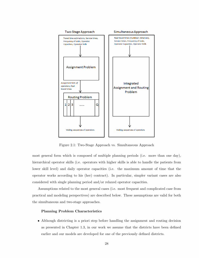
Figure 2.1: Two-Stage Approach vs. Simultaneous Approach
most general form which is composed of multiple planning periods (i.e. more than one day),
hierarchical operator skills (i.e. operators with higher skills is able to handle the patients from
lower skill level) and daily operator capacities (i.e. the maximum amount of time that the
operator works according to his (her) contract). In particular, simpler variant cases are also
considered with single planning period and/or relaxed operator capacities.
Assumptions related to the most general cases (i.e. most frequent and complicated case from
practical and modeling perspectives) are described below. These assumptions are valid for both
the simultaneous and two-stage approaches.
Planning Problem Characteristics
• Although districting is a priori step before handling the assignment and routing decision
as presented in Chapter 1.3, in our work we assume that the districts have been defined
earlier and our models are developed for one of the previously defined districts.
28

• We consider a planning period W (i.e. see for Chapter 1.4 for more details), usually a week
(i.e. Elementary assignment period is a week and elementary routing period is a day, see
Figure 1.5 in Chapter 1) for the models with multiple planning periods .
Patient Characteristics
• Models are defined on a complete directed network G = (N,A) with n nodes, where each
node j corresponds to a patient (with j = 1, . . . , |N |). We assume to have an extra node
(node 0), which is used to denote the common health care center (i.e. basis of the operators)
where each operator starts and comes back for each daily tour.
• A set K of k levels of skill is assumed for patients, where skill k corresponds to the highest
skill (i.e. main skill of the operator) and skill 1 to the lowest level. All the available skill
levels lower than k is also considered as the additional skill of operators.
• Each patient is assumed to have a care plan rj indicating weekly total service requests from
one or more skill levels to be operated according to his/her therapeutic project. In other
words, for each level of skill k, the care plan associated with patient j specifies the number
(frequency) of visits required by patient j in the planning period W relatively to that skill.
Thus, each care plan rj is composed of one or more skill requests and each is denoted by
rjk with k ∈ K, representing the number of visits of skill k required by j in the planning
period.
• It is assumed that the patient requests are operated according to a set P of a priori
given (i.e. input parameters) patterns and they are used to identify all of the possible
visiting combinations. For example, if a patient requires three visits of a given skill in
the planning period, they can be operated according one of the pre-determined patterns
Monday-Wednesday-Friday or Monday-Tuesday-Thursday etc. Formally, for each pattern
p ∈ P we define p(d) = 0 if no service is offered at day d, while it is p(d) = k if a visit of
skill k is operated according to pattern p on day d. Each patient is visited once in the day.
• Each patient j is assumed to have a deterministic demand λj (expressed in time), which
denotes the total amount of care volume (in terms of service and travel time) the patient
requires in the planning period. The demand of patient j is assumed to be calculated as
follows:
29
λj =k∑
k=1
rjk(τj + svj) (2.1)
where svj is the service time that an operator spends at a patient location during a visit.
It is considered as a standard value and without loss of generality, is assumed to have the
same value for all patients. τj is the estimated travel time (or can be replaced with tij
as Euclidean distances) to reach the patient from any other patient or from the common
health care center.
• Each patient receives at most 1 visit per day in total.
• Patient visits do not have precise time windows to be respected.
• We do not consider synchronous visits (i.e. only one operator is simultaneously required
to visit a patient).
Operator Characteristics
• We consider a single category of operators (nurses or doctors).
• Each operator t, t ∈ Ω = 1, ..., O, is assumed to have a deterministic capacity at, which
corresponds to the maximum amount of daily time that he/she works according to his (her)
contract (see Figure 1.6 in Chapter 1).
• The set of available operators on day d, for each d ∈W is denoted by Od.
• HHC operators usually have a main skill and also some additional skills to serve the different
needs of the patients. The main skill of the operator is the one that is best suited to care
a particular patient from a specific category (full knowledge of patient characteristics,
etc.). With the additional skills an operator is also able to handle patients from different
categories in addition to the category of his/her main skill. In this work, we assume a
hierarchical structure of skill levels where an operator with skill k is able to handle all the
requests characterized by a skill level up to k and this is denoted with st. For instance, if
two skill levels are assumed with skill 1 as ordinary (basic) request (non-palliative) and skill
2 as intensive request (palliative). Then, operator t with skill level 2 (i.e. characterized by
st ≥ 1) is able to handle patients from both skill 1 and skill 2 levels. In this thesis, we also
30

assume independent operators skills for some models. If this is the case, operators are only
allowed to handle patients belonging to his/her main skill level.
• Each patient can be assigned to only one operator in the set of existing operators who is
responsible for the care during his/her stay in the HHC service (i.e. Continuity of care is
ensured).
• Each visit requires only one operator.
In this thesis, in the light of these assumptions the assignment and routing problems for
HHC problems are addressed with three types of decision, the care plan scheduling, operator
assignment and routing decisions, for both simultaneous and two-stage approaches. The care
plan scheduling consist in assigning a pattern from P to each patient j to be able to schedule the
requests of a patient j (i.e expressed by rj) during the planning horizon. This is a crucial decision
in the case of several planning days (i.e. multiple planning periods). On the other hand, the
operator assignment decision corresponds to assigning operators to patients for each day where
requests of patients have been scheduled. Lastly, the routing is the decision of computing the
tour of each operator for each scheduled day.
In addressing these decisions, the skill constraints (i.e. the compatibility between the skills
associated with patient requests and the skills of operators) and the daily workload constraints
for the operators are taken into account as well as the continuity of care consideration. Models
are solved under three types of objective functions that are: workload balancing, travel time
minimization and workload balancing/travel time trade-off. Workload balancing refers to the
case where the utilization rates of operators (defined as the ratio between the actual workload
of the operator and his (her) capacity) are to be balanced. The second objective function, cost
minimization, is used to minimize the total traveling times of operators. Lastly, the trade-
off objective function tries to balance the trade off that exists between these two functions
(i.e., workload balancing and travel time minimization). The selection of the objective function
depends on the preference of the HHC service provider as presented in Chapter 1.4.
As a simple case, it is possible to consider the models with single planning period (i.e. a day)
and without operator capacities. Such cases are applicable to real practice as well especially for
small providers (i.e. few operators and small set of patients) or providers working with external
operators. As such, the visiting plan is created one day before the service with the permission
31

of overtime (i.e. no restriction on operator capacities). Overtime is usually allowed when the
operators are paid based on the visiting frequency and not the working time (i.e 8 hours per day).
The single planning period can be easily obtained by assuming W = 1, rj = 1, ∀j ∈ N \ 0 and
P = 1.
In the following parts, first we present the details of the considered models from literature
for the simultaneous approach and then, we provide models that are developed for the two-stage
approach.
32

Part I
THE SIMULTANEOUS APPROACH
33
I.1 INTRODUCTION
As described before, the simultaneous approach (VRP) is used to decide the assignment and
routing decisions at the same time. It is important to note that, since VRP is a well known and
widely studied approach in the literature, in this work, we do not intend to have a significant
contribution to the VRP literature. Rather, we try to use this problem as the benchmark to be
able to analyze the performance of the two-stage approach.
In Section I.2, we first present the literature review for the simultaneous approach of HHC
services. Then, in Section I.3 we provide the general mathematical modeling formulation for this
approach which is developed in a recent work of Cappanera and Scutella [17] where assumptions
such as hierarchical operator skills, and multiple planning periods are considered. We also
formulate other variants of this model by considering independent operator skills and/or single
planning period.
The main contribution of this part is the presentation of the existing model from the literature
(see [17]) and formulation of other variants for benchmark analysis with the models that are
developed for the two-stage approach.
I.2 LITERATURE REVIEW FOR THE SIMULTANEOUS APPROACH
Almost all the existing assignment and routing models in the HHC literature are devoted to the
simultaneous approach. Hence, in this section, we provide a general overview for existing papers
on this topic (see also [26,49]).
This literature review is provided according to the chronological order of the existing works.
Table I.1 provides the overview of the existing works according to the framework provided in
Section 1.4 (see Table 1.1).
Begur et al. [3] propose a Spatial Decision Support System (SDSS) that contains a special
module for the daily scheduling of operators’ activities. This module assigns simultaneously care
providers to visits and generates the sequence in which the visits would be carried out. It is
based on a heuristic approach that combines a set of procedures for building and improving the
daily routes of care providers. The objective of this heuristic is to minimize the total travelling
time while respecting constraints related to the route construction, care providers time windows,
and skills requirements.
34
In the work of Cheng and Rich [21], a daily scheduling problem is developed as a multi-depot
VRP with time windows (VRPTW) and the compability information. The problem is formulated
as a mixed integer linear program. The objective is to minimize the total cost associated with
the amount of overtime hours of full-time nurses and the amount of hours assigned to part-time
nurses. Meanwhile this objective is obtained with respect to visiting each patient exactly once,
assigning each nurse at least one patient, starting and ending at his/her home, taking a lunch
break within the given time interval and respecting the maximum nurse shift length constraints.
The problem is solved by a two-phase heuristic: the first phase falls into the parallel tour-building
procedure category and the second phase attempts to make an improvement on tours identified
in the first phase.
Eveborn et al. [27] develop a decision support system for the local authorities in Sweden,
called Laps Care. In this system, they formulate the scheduling problem as a VRPTW with
the set partitioning model and then solved by a repeated matching algorithm. The objective
is to minimize a total cost related to the travel time, scheduled hours, preferences, etc., while
respecting the following constraints: time windows for visits, operators’ skill requirements, and
accomplishment of each visit by one operator.
Bertels and Fahle [10] propose a weekly plan by using the VRPTW which combines linear
programming, constraint programming, and heuristics in order to assign operators to visits and
sort visits assigned to each operator optimally. The objective is to minimize the total trans-
portation cost while maximizing the satisfaction level of patients and operators with respect to
a variety of soft constraints. These soft constraints include affinities between the patients and
care providers, preferences for certain visits and soft visits’ and care providers’ time windows.
Besides, there are also some hard constraints that must be satisfied: skill requirements, work
time limitations, time window constraints for visits, and the assignment of each visit exactly
once.
Thomsen [47] addresses the daily scheduling problem as a VRPTW and shared visits (visits
by two operators). The objective of this model is to minimize the total travelling cost, the
number of unshared (visit is carried out by a non-reference operator) and unlocked visits and
the number of shared (visit is carried out by two non-reference operators) and unlocked visits.
The constraints of the model are as follows: respecting the visits’ and operators’ time windows,
assignment of at least one visit to each operator and starting, ending a shared visit at the same
35
time. The model is solved by using an insertion heuristic and Tabu search technique.
Akjiratikarl et al. [1] generate daily schedules by using the VRPTW. Since this problem
is a combinatorial optimization problem, they develop a heuristic based approach to solve it.
They develop the Particle Swarm Optimization Problem (PSO) and also incorporate the Local
Improvement Procedure (LIP) into the PSO solution approach to improve their solutions. Finally,
they combine their approach with the Earliest Start Time Priority with Minimum Distance
Assignment technique to generate the initial solutions. Within this framework, they focus on
the determination of routes for each operator while minimizing the total distance travelled with
respect to visits’ and operators’ time windows and assignment of each visit to only one operator.
Ben Bachouch et al. [5] develop the VRP with time windows as a mixed linear programming
model with the objective of minimizing the total distance travelled by the operators. The model
is subject to visits’ and operators’ time windows, nurses’ meal breaks, care continuity and the
restriction on the nurses’ maximum distance travel limit constraints.
Elbenani et al. [25] develop a model for determining routes for operators that incorporates
constraints of the VRP with the medical and continuity of care constraints. Here, each patient is
assigned to a region with respect to his/her home address. Similarly, each nurse is also assigned
to a region but there can be more than one nurse in a specific region. They allow a nurse to
visit a different region with a certain penalty. In this model, they add blood sample related
constraints as a medical constraint and they consider the objective function as minimizing the
total travelling cost of operators. As a final step, they solve this problem with a meta-heuristic
approach based on Tabu search.
Ben Bachouch et al. [6] address the daily drug delivery problem in the French home care
structure as a VRP with time windows. The objective of the model is to minimize the total dis-
tance travelled. In this model they assign carriers to specific regions so that each tour is realized
by the same carrier. In addition, they develop four different strategies as follows: starting deliv-
eries when a specified number of deliveries is received, starting deliveries if a specified distance
is reached regarding to the planned deliveries, starting deliveries on a fixed number of deliveries
per carrier, and starting deliveries on fixed hours. They compare results for each strategy in
order to identify which one is the most efficient to solve the drug delivery problem in the HHC
context.
Chahed et al. [20] couple the production and distribution of anti-cancer drugs within the
36
context of the chemotherapy at home. They present six models based on three main criteria:
time windows, objective function and distribution of drugs. The objective is either to minimize
the delivery cost or maximize the number of visited patients.
Bredstorm and Ronnqvist [12] develop a mathematical model that incorporates synchroniza-
tion and precedence constraints between visits. The proposed model is based on the traditional
VRP with the additional synchronization and precedence constraints. They use a heuristic ap-
proach based on the local branching heuristic to solve their model. In their previous study (see
Bredstorm and Ronnqvist [11]), they developed a branch-and-price algorithm to solve the same
model without including the precedence constraints.
Kergosien et al. [33]) formulate the routing problem of the HHC operators as a Multiple
Traveling Salesman Problem (MTSP) with time windows. The objective of the proposed model
is to minimize the total travelling cost while respecting visits’ and operators’ time windows
constraints, the assignment of each service to one operator constraints, synchronized (some visits
require more than one operator) and disjunctive (some operators cannot work together) services
constraints, continuity of care and the assignment of all operator constraints.
Trautsamwieser et al. [48] develop a model for the daily planning of the HHC services. The
main aim of their work is securing the HHC services in times of natural disasters. They develop
the daily scheduling model as a VRP with state-dependent breaks. The objective of the model
is minimizing the sum of travel times and waiting times, and also the dissatisfaction levels of
the patients and health care operators. The proposed model is first solved for small data with
a state of art solver. Then, they also solve the real life-sized data with a neighborhood search
based heuristic.
Recently, Rasmussen et al. [45] address the daily scheduling problem as a multi-depot VRPTW
and connections between visits. They use a multi-criteria objective rather than only minimizing
the total distance travelled. The proposed formulation is very similar to the one that is developed
by Bredstorm and Ronnqvist [11] but here they allow also a visit to be uncovered (visit is not
carried out). Thus, the proposed multi-criteria objective includes the minimization of uncovered
visits, the maximization of operator-visit preference and the minimization of the total distance
travelling costs. In particular, in the objective function they assign a higher priority to the
uncovered visit criterion than the other criteria. Finally, the constraints of this model include:
each visit can be covered exactly once or left as uncovered, operators can only handle allowed
37

visits, visits’ and operators’ time windows and precedence relations of visits.
Nickel et al. et al. [44] address the weekly scheduling problem as the combination of the
VRPTW and the nurse rostering problem. The objective of the proposed model is minimizing
the weighted sum of the patient-nurse loyalty (continuity of care), unscheduled tasks, the overtime
costs, and the traveling distance. They solve the proposed models using different meta-heuristics
combined with methods from constraint programming which allows a very flexible treatment of
realistic constraints.
Lastly Cappanera and Scutella [17] propose an extended VRP models to formulate the weekly
planning of HHC services by considering skill compatibility between patients and operators. They
develop a hierarchical skill management concept where they allow the over skilled operators to
serve patients with lower skill requirements. The developed model aim at balancing the operator
workload via two objectives with respect to continuity of care and operator skill constraints. The
first considered objective is to maximize the minimum operator utilization factor whereas the
alternative one is to minimize the maximum operator utilization factor. Finally, they analyze
the computational results on a set of real instances.
Note that, the literature on the simultaneous assignment and routing problems is also recently
reviewed by Hulshof et al. [32] that proposes a taxonomic review on planning-related decisions
in health care services, including HHC.
This literature review is provided to present the details of the works that has been provided
for the HHC VRP literature. Table 1.1 presents more specific details of these works as well.
In the following sections, we present the mathematical models for the simultaneous approach
that will be used as the benchmark models for the two-stage models in Chapter 5.
I.3 MATHEMATICAL MODELS
In this section, we present the most general simultaneous model that is considered in this thesis.
The term most general corresponds to the case where hierarchical operator skills, multiple plan-
ning periods and operator capacities are assumed. Then, we also formulate the models where
independent operator skills (i.e. operators assigned only according to their main skill) are con-
sidered. Several alternative models are presented since in practice there are several different
structured health care providers according to their budget, patient and operator profile, region,
country etc. For example, some providers only provide unique service (i.e. blood sample testing)
38
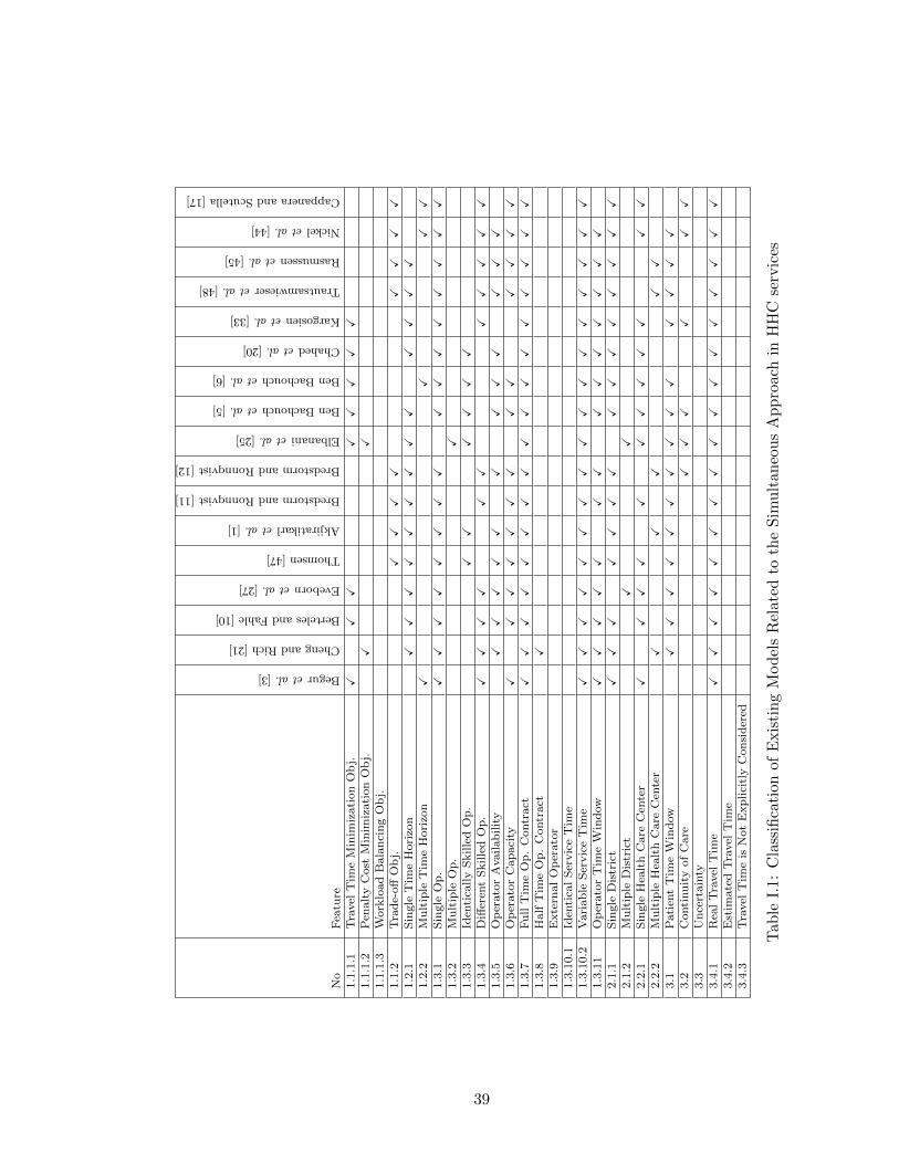
No
Fea
ture
Beguretal.[3]
ChengandRich[21]
BertelesandFahle[10]
Evebornetal.[27]
Thomsen[47]
Akjiratikarletal.[1]
BredstormandRonnqvist[11]
BredstormandRonnqvist[12]
Elbananietal.[25]
BenBachouchetal.[5]
BenBachouchetal.[6]
Chahedetal.[20]
Kargosienetal.[33]
Trautsamwieseretal.[48]
Rasmussenetal.[45]
Nickeletal.[44]
CappaneraandScutella[17]
1.1
.1.1
Tra
vel
Tim
eM
inim
izati
on
Ob
j.X
XX
XX
XX
X1.1
.1.2
Pen
alt
yC
ost
Min
imiz
ati
on
Ob
j.X
X1.1
.1.3
Work
load
Bala
nci
ng
Ob
j.1.1
.2T
rad
e-off
Ob
j.X
XX
XX
XX
X1.2
.1S
ingle
Tim
eH
ori
zon
XX
XX
XX
XX
XX
XX
X1.2
.2M
ult
iple
Tim
eH
ori
zon
XX
XX
1.3
.1S
ingle
Op
.X
XX
XX
XX
XX
XX
XX
XX
X1.3
.2M
ult
iple
Op
.X
1.3
.3Id
enti
cally
Skille
dO
p.
XX
XX
XX
1.3
.4D
iffer
ent
Skille
dO
p.
XX
XX
XX
XX
XX
X1.3
.5O
per
ato
rA
vail
ab
ilit
yX
XX
XX
XX
XX
XX
X1.3
.6O
per
ato
rC
ap
aci
tyX
XX
XX
XX
XX
XX
XX
1.3
.7F
ull
Tim
eO
p.
Contr
act
XX
XX
XX
XX
XX
XX
XX
XX
X1.3
.8H
alf
Tim
eO
p.
Contr
act
X1.3
.9E
xte
rnal
Op
erato
r1.3
.10.1
Iden
tica
lS
ervic
eT
ime
1.3
.10.2
Vari
ab
leS
ervic
eT
ime
XX
XX
XX
XX
XX
XX
XX
XX
X1.3
.11
Op
erato
rT
ime
Win
dow
XX
XX
XX
XX
XX
XX
XX
2.1
.1S
ingle
Dis
tric
tX
XX
XX
XX
XX
XX
XX
XX
2.1
.2M
ult
iple
Dis
tric
tX
X2.2
.1S
ingle
Hea
lth
Care
Cen
ter
XX
XX
XX
XX
XX
XX
2.2
.2M
ult
iple
Hea
lth
Care
Cen
ter
XX
XX
X3.1
Pati
ent
Tim
eW
ind
ow
XX
XX
XX
XX
XX
XX
XX
3.2
Conti
nu
ity
of
Care
XX
XX
XX
3.3
Un
cert
ain
ty3.4
.1R
eal
Tra
vel
Tim
eX
XX
XX
XX
XX
XX
XX
XX
XX
3.4
.2E
stim
ate
dT
ravel
Tim
e3.4
.3T
ravel
Tim
eis
Not
Exp
lici
tly
Con
sid
ered
Tab
leI.
1:C
lass
ifica
tion
ofE
xis
tin
gM
od
els
Rel
ated
toth
eS
imult
aneo
us
Ap
pro
ach
inH
HC
serv
ices
39

to their patients thus, a model with independent operator skill for multiple planning periods is
required to be able to formulate such case. On the other, some providers serve patients with
regular (non-palliative patients) or intensive (palliative patients) service requirements. Hence,
such case can be formulated with a model considering the hierarchical skills either for multiple
or single planning period.
In order to formulate the HHC models in a more formal way, let us recall or define the
following definitions:
W the planning period
K the set of skill levels
k the highest skill
rjk the number of visits required by patient j in W from skill k, j ∈ N(j 6= 0), k ∈ K
svj the service time that an operator spends at the location of patient j
tij the traveling time from patient i to j, (i, j) ∈ A
at the daily capacity of operator t, t ∈ O
Od the set of available operators on day d, for each d ∈W
Dtd the daily workload of operator t, t ∈ Od, d ∈W
The following variables are used to model the care plan scheduling, the assignment and the
routing decisions:
zjp =
1 if pattern p is assigned to patient j
0 otherwisej ∈ N \ 0, p ∈ P
utj =
1 if operator t is assigned to patient j
0 otherwiset ∈ O, j ∈ N \ 0
xtdij =
1 if operator t travels along (i, j) on day d
0 otherwise(i, j) ∈ A, i 6= j, d ∈W , t ∈ Od
and
40

ydij auxiliary flow variable which represents the number of the patients visited after patient i
by the operator moving along (i, j) on day d, (i, j) ∈ A, d ∈W .
Using these variables and definitions, in the following section we present the simultaneous
hierarchical skill model (see [17]). Then, variant of this model with independent skills is formu-
lated. For both cases, variant models including multiple and single planning periods with and
without capacity constraints are also presented.
I.3.1 Hierarchical Skill, Multiple Planning Periods Model
Remind that the hierarchical skill corresponds to the case where an operator with skill k is able
to handle all the requests characterized by a skill level up to k. In particular, multiple planning
periods are defined as W ≥ 2.
In this case, it is assumed that the previously mentioned three decisions are considered
simultaneously for all patient types (i.e., with all required skill levels) and for all skill levels
of operators via a joint approach. In other words, a single simultaneous problem is formulated
involving all operators (i.e. from each skill level), to handle all the patient requirements from each
skill level with the use of the hierarchical skill consideration. This refers to the case where more
qualified operator, e.g. with skill level k = 2, is assumed to serve patients that belong to either
skill k = 1 and/or skill k = 2 levels. This hierarchical skill consideration for the simultaneous
approach with the workload balancing objective is given by the following model:
41

min h (2.2)∑i∈N
∑t∈O
xtdij ≤∑
p:p(d)≥1
zjp ∀j ∈ N \ 0, ∀d ∈W (2.3)
∑i∈N
∑t∈st≥k
xtdij ≥∑
p:p(d)=k
zjp ∀j ∈ N \ 0, ∀d ∈W, ∀k ∈ K (2.4)
∑p∈P
zjp = 1 ∀j ∈ N \ 0 (2.5)
∑t∈O
utj = 1 ∀j ∈ N \ 0 (2.6)
xtdij ≤ utj ∀(i, j) ∈ A,∀j ∈ N \ 0,∀d ∈W, ∀t ∈ Od (2.7)
utj ≤∑i∈N
∑d∈W
xtdij ∀j ∈ N \ 0, ∀t ∈ O (2.8)
Dtd =∑
(i,j)∈A
(tij + svj) · xtdij ≤ at ∀d ∈W, ∀t ∈ Od (2.9)
∑i∈N
xtdij =∑i∈N
xtdji ∀j ∈ N \ 0, ∀d ∈W, ∀t ∈ Od (2.10)
∑j∈N
yd0j =∑
j∈N\0
∑p:p(d)≥1
zjp ∀d ∈W (2.11)
∑i∈N
ydij −∑i∈N
ydji =∑
p:p(d)≥1
zjp ∀j ∈ N \ 0, ∀d ∈W (2.12)
ydij ≤ n∑t∈Od
xtdij ∀(i, j) ∈ A,∀d ∈W (2.13)∑d∈W Dtd
|W | · at≤ h ∀t ∈ O (2.14)
Constraint (2.3) states that (exactly) one operator per day can visit patient j only if a visit
has been scheduled on that day for node j. Constraint (2.4) guarantees that, on day d, exactly
one operator, of adequate skill, must visit patient j if a service of that skill has been scheduled
for j on day d. In particular, the least skilled operators can perform only visits of skill 1 (case
k = 1), whereas the most skilled operators can perform all types of visits (case k = k). Constraint
(2.5) ensures that each patient is assigned exactly to one pattern. Constraint (2.6) ensures that
exactly one operator is assigned to each patient during the planning period. This is included in
order to guarantee the continuity of care. Constraint (2.7) guarantees that an operator can visit
42

a patient only if he/she has been assigned to that patient (links between routing and assignment
variables). Furthermore, constraint (2.8) forces variables utj to zero if operator t never visits
patient j during the planning period. Constraint (2.9) ensures that the workload of each operator
in each day, expressed as the sum of the service times and the traveling times, does not exceed the
corresponding daily capacity. Constraint (2.10) is the classical flow conservation constraint on
the routing variables. Constraint (2.11) and (2.12) are the flow conservation constraints on the
auxiliary y variables, which are introduced to avoid sub-tours in solutions. They also guarantee
the link between scheduling decisions and auxiliary flow variables. Finally, constraints (2.13)
link together routing variables and auxiliary flow variables.
Note that a pattern variable zjp can have a value other than zero only if:
|d : p(d) = k| = rjk ∀k ∈ K. (2.15)
Therefore, in the preprocessing step zjp = 0 if anyone of the k constraints (2.15) is not
satisfied. In addition, in the preprocessing step xtdij = 0 if patients i and j have only requests of
skill at least k during the planning horizon, and t is an operator of skill less than k (i.e. st ≤ k).
The objective function defines a workload balancing between operators over the planning
period by minimizing the maximum operator utilization rate.
An alternative objective function considers the cost minimization where total travel time of
operators are considered like in the classical VRP model. The model with the cost minimization
can be formulated as follows:
min v (2.16)
Constraints (2.3)− (2.13) (2.17)∑d∈W
∑(i,j)∈A
tij · xtdij = v ∀t ∈ O, (2.18)
where the auxiliary variable v defines the total traveling time of operators in the planning period.
The last alternative objective functions is defined as the trade-off function that balances the
trade-off that exists between workload balancing and total travel time minimization. This case
is defined as follows:
43
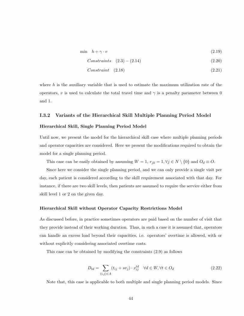
min h+ γ · v (2.19)
Constraints (2.3)− (2.14) (2.20)
Constraint (2.18) (2.21)
where h is the auxiliary variable that is used to estimate the maximum utilization rate of the
operators, v is used to calculate the total travel time and γ is a penalty parameter between 0
and 1.
I.3.2 Variants of the Hierarchical Skill Multiple Planning Period Model
Hierarchical Skill, Single Planning Period Model
Until now, we present the model for the hierarchical skill case where multiple planning periods
and operator capacities are considered. Here we present the modifications required to obtain the
model for a single planning period.
This case can be easily obtained by assuming W = 1, rjk = 1, ∀j ∈ N \ 0 and Od ≡ O.
Since here we consider the single planning period, and we can only provide a single visit per
day, each patient is considered according to the skill requirement associated with that day. For
instance, if there are two skill levels, then patients are assumed to require the service either from
skill level 1 or 2 on the given day.
Hierarchical Skill without Operator Capacity Restrictions Model
As discussed before, in practice sometimes operators are paid based on the number of visit that
they provide instead of their working duration. Thus, in such a case it is assumed that, operators
can handle an excess load beyond their capacities, i.e. operators’ overtime is allowed, with or
without explicitly considering associated overtime costs.
This case can be obtained by modifying the constraints (2.9) as follows
Dtd =∑
(i,j)∈A
(tij + svj) · xtdij ∀d ∈W, ∀t ∈ Od (2.22)
Note that, this case is applicable to both multiple and single planning period models. Since
44
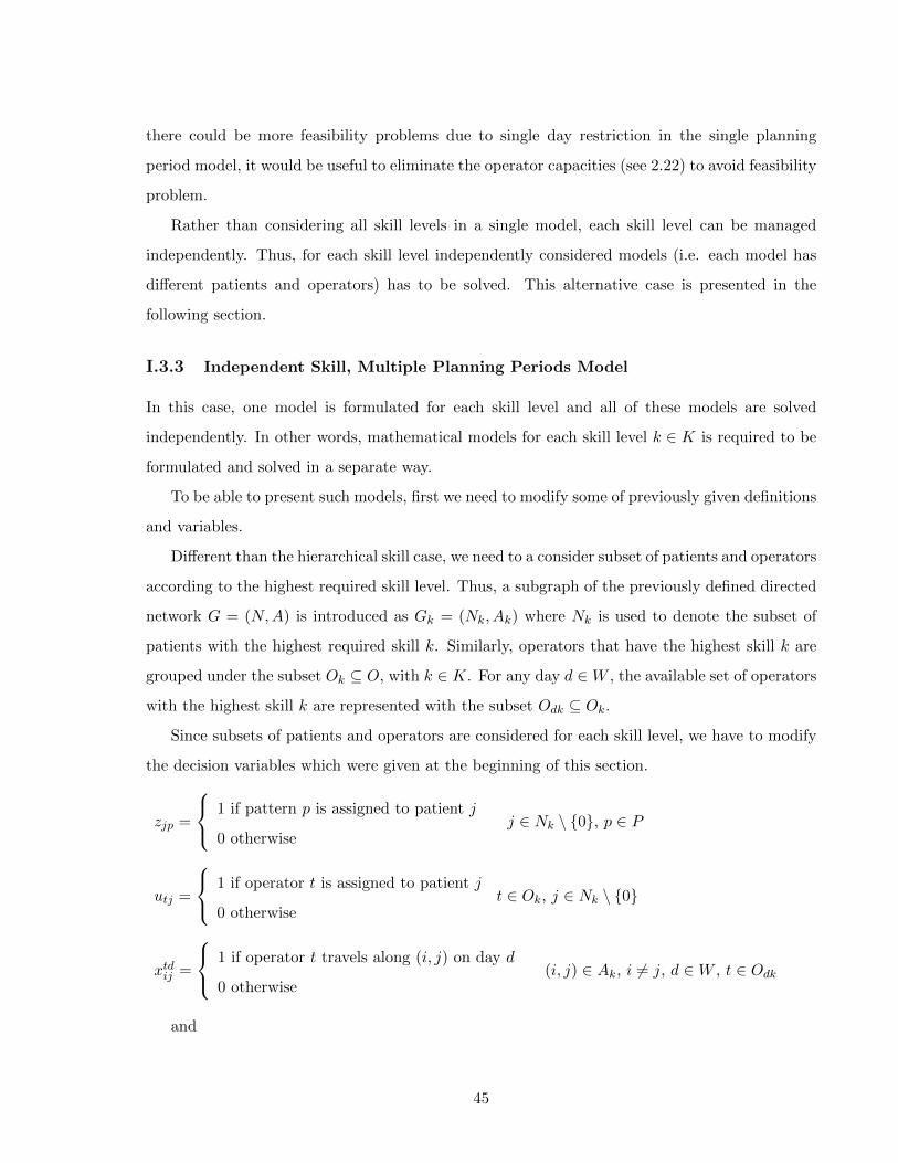
there could be more feasibility problems due to single day restriction in the single planning
period model, it would be useful to eliminate the operator capacities (see 2.22) to avoid feasibility
problem.
Rather than considering all skill levels in a single model, each skill level can be managed
independently. Thus, for each skill level independently considered models (i.e. each model has
different patients and operators) has to be solved. This alternative case is presented in the
following section.
I.3.3 Independent Skill, Multiple Planning Periods Model
In this case, one model is formulated for each skill level and all of these models are solved
independently. In other words, mathematical models for each skill level k ∈ K is required to be
formulated and solved in a separate way.
To be able to present such models, first we need to modify some of previously given definitions
and variables.
Different than the hierarchical skill case, we need to a consider subset of patients and operators
according to the highest required skill level. Thus, a subgraph of the previously defined directed
network G = (N,A) is introduced as Gk = (Nk, Ak) where Nk is used to denote the subset of
patients with the highest required skill k. Similarly, operators that have the highest skill k are
grouped under the subset Ok ⊆ O, with k ∈ K. For any day d ∈W , the available set of operators
with the highest skill k are represented with the subset Odk ⊆ Ok.
Since subsets of patients and operators are considered for each skill level, we have to modify
the decision variables which were given at the beginning of this section.
zjp =
1 if pattern p is assigned to patient j
0 otherwisej ∈ Nk \ 0, p ∈ P
utj =
1 if operator t is assigned to patient j
0 otherwiset ∈ Ok, j ∈ Nk \ 0
xtdij =
1 if operator t travels along (i, j) on day d
0 otherwise(i, j) ∈ Ak, i 6= j, d ∈W , t ∈ Odk
and
45
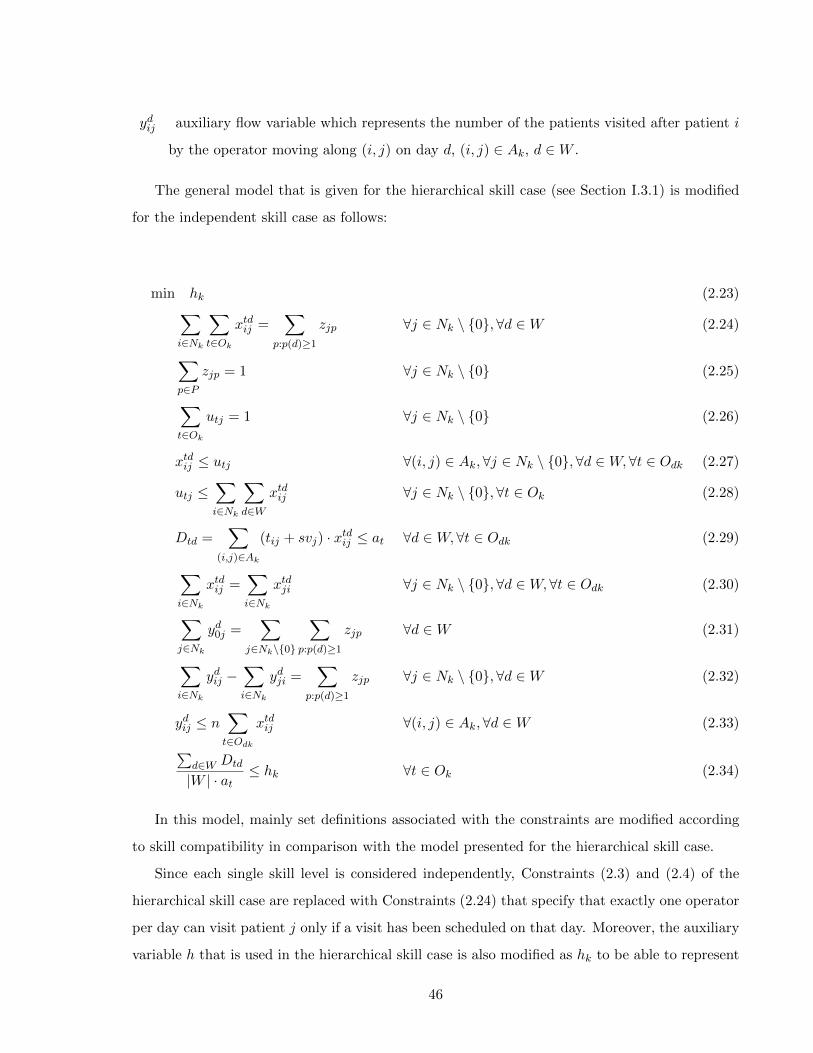
ydij auxiliary flow variable which represents the number of the patients visited after patient i
by the operator moving along (i, j) on day d, (i, j) ∈ Ak, d ∈W .
The general model that is given for the hierarchical skill case (see Section I.3.1) is modified
for the independent skill case as follows:
min hk (2.23)∑i∈Nk
∑t∈Ok
xtdij =∑
p:p(d)≥1
zjp ∀j ∈ Nk \ 0, ∀d ∈W (2.24)
∑p∈P
zjp = 1 ∀j ∈ Nk \ 0 (2.25)
∑t∈Ok
utj = 1 ∀j ∈ Nk \ 0 (2.26)
xtdij ≤ utj ∀(i, j) ∈ Ak,∀j ∈ Nk \ 0,∀d ∈W, ∀t ∈ Odk (2.27)
utj ≤∑i∈Nk
∑d∈W
xtdij ∀j ∈ Nk \ 0, ∀t ∈ Ok (2.28)
Dtd =∑
(i,j)∈Ak
(tij + svj) · xtdij ≤ at ∀d ∈W, ∀t ∈ Odk (2.29)
∑i∈Nk
xtdij =∑i∈Nk
xtdji ∀j ∈ Nk \ 0, ∀d ∈W, ∀t ∈ Odk (2.30)
∑j∈Nk
yd0j =∑
j∈Nk\0
∑p:p(d)≥1
zjp ∀d ∈W (2.31)
∑i∈Nk
ydij −∑i∈Nk
ydji =∑
p:p(d)≥1
zjp ∀j ∈ Nk \ 0, ∀d ∈W (2.32)
ydij ≤ n∑t∈Odk
xtdij ∀(i, j) ∈ Ak,∀d ∈W (2.33)∑d∈W Dtd
|W | · at≤ hk ∀t ∈ Ok (2.34)
In this model, mainly set definitions associated with the constraints are modified according
to skill compatibility in comparison with the model presented for the hierarchical skill case.
Since each single skill level is considered independently, Constraints (2.3) and (2.4) of the
hierarchical skill case are replaced with Constraints (2.24) that specify that exactly one operator
per day can visit patient j only if a visit has been scheduled on that day. Moreover, the auxiliary
variable h that is used in the hierarchical skill case is also modified as hk to be able to represent
46
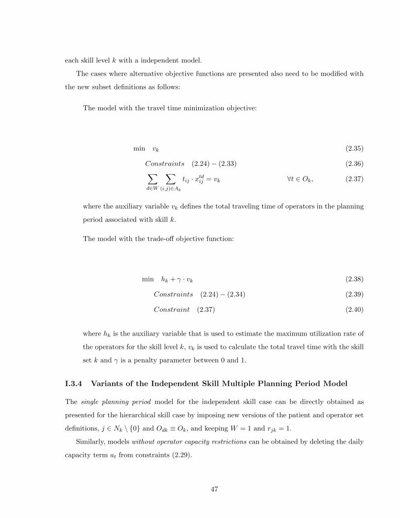
each skill level k with a independent model.
The cases where alternative objective functions are presented also need to be modified with
the new subset definitions as follows:
The model with the travel time minimization objective:
min vk (2.35)
Constraints (2.24)− (2.33) (2.36)∑d∈W
∑(i,j)∈Ak
tij · xtdij = vk ∀t ∈ Ok, (2.37)
where the auxiliary variable vk defines the total traveling time of operators in the planning
period associated with skill k.
The model with the trade-off objective function:
min hk + γ · vk (2.38)
Constraints (2.24)− (2.34) (2.39)
Constraint (2.37) (2.40)
where hk is the auxiliary variable that is used to estimate the maximum utilization rate of
the operators for the skill level k, vk is used to calculate the total travel time with the skill
set k and γ is a penalty parameter between 0 and 1.
I.3.4 Variants of the Independent Skill Multiple Planning Period Model
The single planning period model for the independent skill case can be directly obtained as
presented for the hierarchical skill case by imposing new versions of the patient and operator set
definitions, j ∈ Nk \ 0 and Odk ≡ Ok, and keeping W = 1 and rjk = 1.
Similarly, models without operator capacity restrictions can be obtained by deleting the daily
capacity term at from constraints (2.29).
47

Note that if we consider the independent skill case (i.e. for any skill level k) for a single
planning period and without capacity restrictions then, this model turns out to be the well-
known Multiple Traveling Salesman Problem (MTSP) that has been extensively studied in the
VRP domain (for more details please refer to [4]).
48

Part II
THE TWO-STAGE APPROACH
49
II.1 INTRODUCTION
In this part, we present an alternative approach for solving the assignment and routing problems
of HHC services. As presented before, in this procedure first the assignment problem, and then,
the routing problem are solved independently. Note that, to the best our of knowledge there is
no work related to the two-stage approach for the assignment and routing problems in the HHC
literature. Thus, with this part, we contribute to the related HHC literature by providing a new
two-stage approach concerning several variants of the assignment and routing problems.
Several new models for the two-stage approach for the hierarchical and independent skill cases
are developed for single or multiple planning periods. Since the visiting sequences for operators
are not known in the assignment phase of these models, an estimation τj for the travel times is
required to be able solve the assignment and routing problems with the two-stage approach. To
this end, different travel times estimation methods are considered and presented in Chapter 3.
Remind that in the multiple planing period case (i.e. W ≥ 2), in addition to the Assignment
(A) and Routing (R) decision, we also need to consider the Care Plan (CP) decision (i.e. pattern
assignment). In the two-stage approach, this decision can be incorporated via three alternative
scenarios. The first one (i.e. Model II) is solving the assignment model for the whole planning
period W by considering all patient service requirements but without deciding the care plan
schedules of the patients (i.e. no pattern assignment). Then, with the assignment decisions from
the first stage, routing models with care plan decision is required to be solved for each operator.
The second alternative (i.e. Model III) is simultaneously deciding the assignment and care plan
decision and then solving several routing models for each day and for each operator. The last
scenario (i.e. Model IV) is the combination of these two previous alternatives where care plan
decision is incorporated into both stages of the two-stage approach. To present complete schema,
we provide Figure II.1 with all alternative cases for models with multiple planning periods as
well as the model with the single planning period (i.e. Model I).
All these models are important to analyze several scenarios encountered in the two-stage
approach especially for the multiple planning periods. For example, Model II and Model III are
useful to analyze when to make the care plan decision to be able to obtain solutions close to
the ones obtained from the simultaneous approach. Particularly, Model IV can be considered
as the combination of the Model II and III where the care plan decision that is obtained in the
assignment stage is modified in the routing stage. This model (Model IV) might be useful to
50
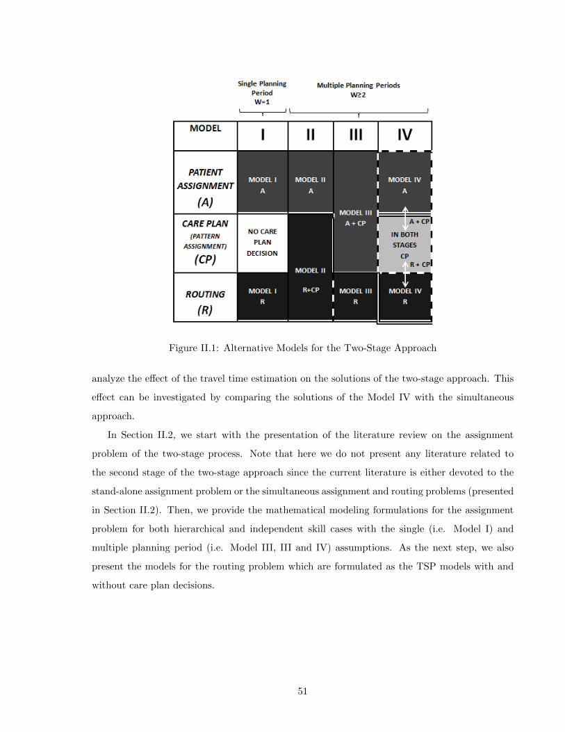
Figure II.1: Alternative Models for the Two-Stage Approach
analyze the effect of the travel time estimation on the solutions of the two-stage approach. This
effect can be investigated by comparing the solutions of the Model IV with the simultaneous
approach.
In Section II.2, we start with the presentation of the literature review on the assignment
problem of the two-stage process. Note that here we do not present any literature related to
the second stage of the two-stage approach since the current literature is either devoted to the
stand-alone assignment problem or the simultaneous assignment and routing problems (presented
in Section II.2). Then, we provide the mathematical modeling formulations for the assignment
problem for both hierarchical and independent skill cases with the single (i.e. Model I) and
multiple planning period (i.e. Model III, III and IV) assumptions. As the next step, we also
present the models for the routing problem which are formulated as the TSP models with and
without care plan decisions.
51
II.2 LITERATURE REVIEW ON THE ASSIGNMENT MODELS
As in the previous literature review presented in SectionI.2, the overview of the existing works
is also provided for the stand-alone assignment problem in Table II.1.
The assignment problem in the HHC literature has been rarely studied as a stand-alone
problem (i.e. without considering the routing problem). Hertz and Lahrichi [30] propose two
different mixed integer programming models for assigning operators to patients. The objective
of both models is to balance the nurses’ workloads by minimizing a weighted sum of the visit
load (based on the weight of each visit), the case load (due to the number of patients assigned)
and the travel load (related to the distances traveled) while respecting constraints related to
maximum acceptable loads and continuity of care. The travel load is calculated on the basis
of the average distance of the patient location from the district where operator works. Since
the estimate does not consider sequencing, it should be accurate for small districts. Borsani et
al. [15] propose assignment and scheduling models where the output of the assignment model
is incorporated as the input to the scheduling model. In this work, the assignment process is
held to ensure workload balance among operators while respecting continuity of care, qualification
requirements and geographical coherence constraints. Travel times are constant and independent
from the sequence.
An extended modeling framework related to the assignment problems of the HHC services
was developed by Lanzarone et al. [36], where the authors provide different assignment models
to balance the operators’ workloads by considering several peculiarities of HHC services, such
as the operators’ skills, the geographical locations of patients and operators, and the stochastic
patient requests. Travel times are modeled as in [15]. The same problem with stochastic demand
is then tackled in the works of Lanzarone and Matta [35, 37] who propose simple policies to
assign patients to operators instead of mathematical programming. Carello and Lanzarone [18]
develop a cardinality–constrained robust assignment model where their aim is to exploit the
potentialities of a mathematical programming formulation and to evaluate the capability of such
model in reducing the costs related to nurses’ overtimes. Also in this case, the travel time for
reaching homes is the same for all the patients and operators. Lastly, Koeleman et al. [34]
represent the HHC system as a Markov chain and they develop admittance policies for patients
with the use of a trunk reservation heuristic to control the system by considering a general
visiting time containing a travel load that does not consider routes.
52
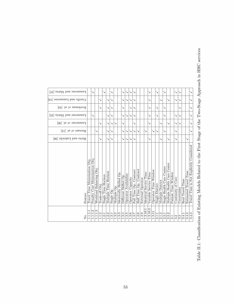
No
Fea
ture
HertzandLahrichi[30]
Borsanietal.[15]
Lanzaroneetal.[36]
LanzaroneandMatta[35]
Koelemanetal.[34]
CarelloandLanzarone[18]
LanzaroneandMatta[37]
1.1
.1.1
Tra
vel
Tim
eM
inim
izati
on
Ob
j.1.1
.1.2
Pen
alt
yC
ost
Min
imiz
ati
on
Ob
j.X
X1.1
.1.3
Work
load
Bala
nci
ng
Ob
j.X
1.1
.2T
rad
e-off
Ob
j.X
XX
X1.2
.1S
ingle
Tim
eH
ori
zon
X1.2
.2M
ult
iple
Tim
eH
ori
zon
XX
XX
XX
1.3
.1S
ingle
Op
.X
XX
XX
XX
1.3
.2M
ult
iple
Op
.X
1.3
.3Id
enti
cally
Skille
dO
p.
1.3
.4D
iffer
ent
Skille
dO
p.
XX
XX
XX
X1.3
.5O
per
ato
rA
vail
abil
ity
XX
XX
X1.3
.6O
per
ato
rC
ap
aci
tyX
XX
XX
X1.3
.7F
ull
Tim
eO
p.
Contr
act
XX
XX
XX
X1.3
.8H
alf
Tim
eO
p.
Contr
act
X1.3
.9E
xte
rnal
Op
erato
r1.3
.10.1
Iden
tica
lS
ervic
eT
ime
X1.3
.10.2
Vari
ab
leS
ervic
eT
ime
XX
XX
XX
1.3
.11
Op
erato
rT
ime
Win
dow
X2.1
.1S
ingle
Dis
tric
tX
XX
X2.1
.2M
ult
iple
Dis
tric
tX
XX
2.2
.1S
ingle
Hea
lth
Care
Cen
ter
XX
XX
2.2
.2M
ult
iple
Hea
lth
Care
Cen
ter
XX
X3.1
Pati
ent
Tim
eW
ind
ow
3.2
Conti
nu
ity
of
Care
XX
XX
XX
3.3
Un
cert
ain
tyX
XX
XX
3.4
.1R
eal
Tra
vel
Tim
e3.4
.2E
stim
ate
dT
ravel
Tim
eX
3.4
.3T
ravel
Tim
eis
Not
Exp
lici
tly
Con
sid
ered
XX
XX
XX
Tab
leII
.1:
Cla
ssifi
cati
on
of
Exis
tin
gM
od
els
Rel
ated
toth
eF
irst
Sta
geof
the
Tw
o-S
tage
Ap
pro
ach
inH
HC
serv
ices
53
A common characteristics of the assignment related papers is the need of balancing the
workload among operators. Indeed, this problem is extremely important to have equal working
conditions in the same organization. However, these papers does not consider the hierarchical
skills and they do not focus on the travel time estimation methods. These are two important
issues that has to be considered to be able to better reflect the real cases. To this end, in
the following sections, we present new mathematical models with hierarchical skills that we have
developed for the assignment problem of the two-stage approach. Then, in Chapter 3, we provide
different travel time estimation methods.
II.3 PROPOSED MATHEMATICAL MODELS FOR THE ASSIGNMENT PROB-
LEM
In this section, we present the models that are developed for the first stage of the two-stage
approach. As shown in Figure II.1, single and multiple planning period cases are considered for
the assignment problem. In particular, for the multiple planning period case, two main models
are developed where in the first one the assignment decision is held with the care plan decision
(i.e. Model III and IV) whereas in the second one only the assignment decision is considered
(i.e. Model I and II) and the care plan decision is left for the routing stage. Furthermore, all
these models are investigated under two skill cases, hierarchical and independent skills, as in the
simultaneous approach.
In the literature of the assignment models for HHC services, there are works that considers
different operator skills however, there is no work that focus on the management of the skills
independently or hierarchically. In particular, considering the care plan decision within the
assignment problem is also new to the literature.
In this section, models are presented mainly based on definitions, notations and variables
given for the simultaneous approach. The only new variable is defined as follows:
µtdj =
1 if operator t is assigned to patient j on day d
0 otherwisej ∈ N \ 0, d ∈W , t ∈ O
Note that this notation is provided only for the hierarchical skill case. In the independent
skill case, the given set definitions are modified as j ∈ Nk \ 0 for patients and t ∈ Ok for
operators.
54
II.3.1 Hierarchical Skill Case
We first start by presenting the models with multiple planning periods (see Model II (A), Model
III (A+CP) and Model IV (A+CP)) in Figure II.1). As detailed before, two alternative modeling
structures are proposed where the first one includes simultaneous assignment and care plan
decisions (Model III (AC+P) and Model IV (AC+P)) and the second one is only based on the
assignment decision (Model II (A)). The main difference between these models lies on the care
plan decision which is included in the assignment stage of Model III and IV and not considered
in the assignment stage of Model II.
1. Model III (A+CP) and Model IV (A+CP) with Hierarchical Skills
Model III (A+CP) and Model IV (A+CP) is represented with the same assignment model
where care plan decision is also made. The aim of the model is to assign patients to
operators with the daily scheduling information (e.g. Patient 3 (with 2 visit requirements)
is assigned to the Operator 1 and the visits are scheduled on Monday and Thursday).
The formulation of this model is given as follows:
55
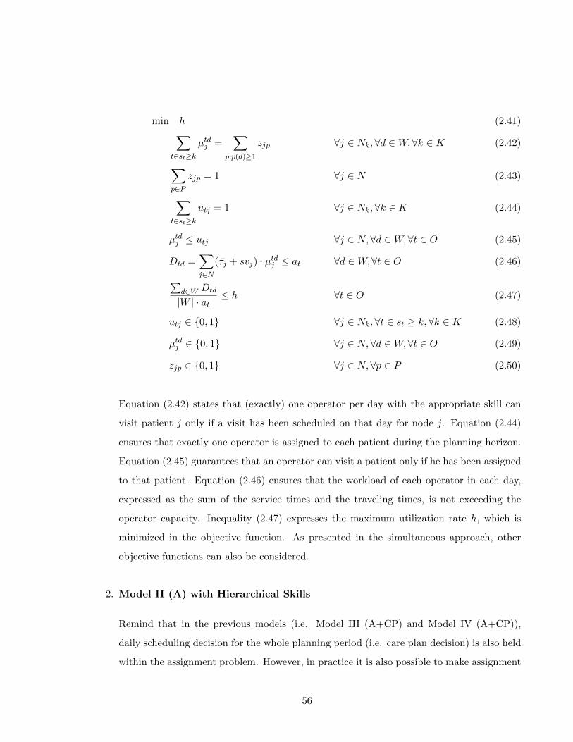
min h (2.41)∑t∈st≥k
µtdj =∑
p:p(d)≥1
zjp ∀j ∈ Nk,∀d ∈W, ∀k ∈ K (2.42)
∑p∈P
zjp = 1 ∀j ∈ N (2.43)
∑t∈st≥k
utj = 1 ∀j ∈ Nk,∀k ∈ K (2.44)
µtdj ≤ utj ∀j ∈ N, ∀d ∈W, ∀t ∈ O (2.45)
Dtd =∑j∈N
(τj + svj) · µtdj ≤ at ∀d ∈W, ∀t ∈ O (2.46)∑d∈W Dtd
|W | · at≤ h ∀t ∈ O (2.47)
utj ∈ 0, 1 ∀j ∈ Nk,∀t ∈ st ≥ k, ∀k ∈ K (2.48)
µtdj ∈ 0, 1 ∀j ∈ N, ∀d ∈W, ∀t ∈ O (2.49)
zjp ∈ 0, 1 ∀j ∈ N, ∀p ∈ P (2.50)
Equation (2.42) states that (exactly) one operator per day with the appropriate skill can
visit patient j only if a visit has been scheduled on that day for node j. Equation (2.44)
ensures that exactly one operator is assigned to each patient during the planning horizon.
Equation (2.45) guarantees that an operator can visit a patient only if he has been assigned
to that patient. Equation (2.46) ensures that the workload of each operator in each day,
expressed as the sum of the service times and the traveling times, is not exceeding the
operator capacity. Inequality (2.47) expresses the maximum utilization rate h, which is
minimized in the objective function. As presented in the simultaneous approach, other
objective functions can also be considered.
2. Model II (A) with Hierarchical Skills
Remind that in the previous models (i.e. Model III (A+CP) and Model IV (A+CP)),
daily scheduling decision for the whole planning period (i.e. care plan decision) is also held
within the assignment problem. However, in practice it is also possible to make assignment
56
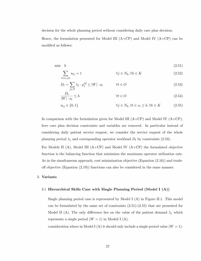
decision for the whole planning period without considering daily care plan decision.
Hence, the formulation presented for Model III (A+CP) and Model IV (A+CP) can be
modified as follows:
min h (2.51)∑t∈st≥k
utj = 1 ∀j ∈ Nk, ∀k ∈ K (2.52)
Dt =∑j∈N
λj · µtdj ≤ |W | · at ∀t ∈ O (2.53)
Dt
|W | · at≤ h ∀t ∈ O (2.54)
utj ∈ 0, 1 ∀j ∈ Nk, ∀t ∈ st ≥ k,∀k ∈ K (2.55)
In comparison with the formulation given for Model III (A+CP) and Model IV (A+CP),
here care plan decision constraints and variables are removed. In particular instead of
considering daily patient service request, we consider the service request of the whole
planning period λj and corresponding operator workload Dt by constraints (2.53).
For Models II (A), Model III (A+CP) and Model IV (A+CP) the formulated objective
function is the balancing function that minimizes the maximum operator utilization rate.
As in the simultaneous approach, cost minimization objective (Equation (2.16)) and trade-
off objective (Equation (2.19)) functions can also be considered in the same manner.
3. Variants
3.1 Hierarchical Skills Case with Single Planning Period (Model I (A))
Single planning period case is represented by Model I (A) in Figure II.1. This model
can be formulated by the same set of constraints (2.51)-(2.55) that are presented for
Model II (A). The only difference lies on the value of the patient demand λj which
represents a single period (W = 1) in Modeil I (A).
consideration where in Model I (A) it should only include a single period value (W = 1).
57
3.2 Hierarchical Skills Case without Operator Capacity Restrictions
The capacity restrictions of operators can be relaxed by omitting the right-hand-side
terms ≤ at from equation (2.46) and ≤ |W | · at from equation (2.52).
All models presented with the hierarchical skill case are also applicable to the independent
skill case. The following part presents the details of Model I (A), Model II (A), Model III (A+CP)
and Model IV (A+CP) for the independent skill case.
II.3.2 Independent Skill Case
As discussed in Section I.3.3, k (i.e. the number of available skill level) models are required to be
able to manage each skill level independently. Set definitions, notations and variables presented
in Section I.3.3 are also valid for this case. The set definition of the assignment variable µtdj that
is presented in the previous section is modified according to independent skill compatibility and
this modification is presented in the model formulation.
Here below, we first present the developed model with the multiple planning periods (Model
II (A), Model III (A+CP) and Model IV (A+CP)), and then, the model with the single planning
period (Model I) respectively.
1. Model III (A+CP) and Model IV (A+CP) with Independent Skills
Remind that Model III (A+CP) and Model IV (A+CP) represents the case where the
assignment decision is held simultaneously with the care plan decision for multiple periods.
The corresponding formulation with independent skills (i.e. for each skill level k) and the
balancing objective are shown as follows:
58
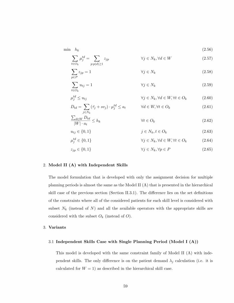
min hk (2.56)∑t∈Ok
µtdj =∑
p:p(d)≥1
zjp ∀j ∈ Nk,∀d ∈W (2.57)
∑p∈P
zjp = 1 ∀j ∈ Nk (2.58)
∑t∈Ok
utj = 1 ∀j ∈ Nk (2.59)
µtdj ≤ utj ∀j ∈ Nk,∀d ∈W, ∀t ∈ Ok (2.60)
Dtd =∑j∈Nk
(τj + svj) · µtdj ≤ at ∀d ∈W, ∀t ∈ Ok (2.61)∑d∈W Dtd
|W | · at≤ hk ∀t ∈ Ok (2.62)
utj ∈ 0, 1 j ∈ Nk, t ∈ Ok (2.63)
µtdj ∈ 0, 1 ∀j ∈ Nk,∀d ∈W, ∀t ∈ Ok (2.64)
zjp ∈ 0, 1 ∀j ∈ Nk,∀p ∈ P (2.65)
2. Model II (A) with Independent Skills
The model formulation that is developed with only the assignment decision for multiple
planning periods is almost the same as the Model II (A) that is presented in the hierarchical
skill case of the previous section (Section II.3.1). The difference lies on the set definitions
of the constraints where all of the considered patients for each skill level is considered with
subset Nk (instead of N) and all the available operators with the appropriate skills are
considered with the subset Ok (instead of O).
3. Variants
3.1 Independent Skills Case with Single Planning Period (Model I (A))
This model is developed with the same constraint family of Model II (A) with inde-
pendent skills. The only difference is on the patient demand λj calculation (i.e. it is
calculated for W = 1) as described in the hierarchical skill case.
59
Note that all of previously presented alternative objective functions are applicable to
the models of the independent skill case as well.
3.2 Independent Skills Case without Operator Capacity Restrictions
The operator capacity relation can also be obtained as it is presented in the hierarchical
skill case of the two-stage approach.
Till now we have only presented the models for the first stage of the two-stage approach
where we obtain either the assignment or the assignment and care plan decisions. In the following
section, we present the details of the second-stage models where the visiting sequences of the
operators are obtained.
II.4 MATHEMATICAL MODELS FOR THE ROUTING PROBLEM
At this level of the two-stage approach, TSP models are used to create each operator’s route
with the information obtained from the assignment step for the given planning period.
Different than the existing routing models in the HHC services, here the stand alone routing
problem with the care plan decision is formulated. In particular, travel time balancing among
operators with the already assigned patients is also new to this literature.
As presented in Figure II.1, similar to the assignment decision, the routing decision can be
held with (Model II (R+CP) and Model IV (R+CP)) or without the care plan decision (Model
I (R) and Model III (R)). In this thesis, these cases are formulated with two TSP formulations
(with care plan decision (R+CP) or without care plan decision (R)) independent from the skill
compatibility issue. The first mathematical formulations is used to consider Model II (R+CP)
and Model IV (R+CP) where the routing decision is held with the care plan decision. The other
formulation is considered for the stand-alone routing decision to be able to solve Model I (R)
and Model III (R).
Since the operator to patient assignment has already been decided according to the appro-
priate skill configuration in the first stage of the problem, this issue is not incorporated into the
routing models.
In this part, we need to reconsider the previously given definitions, notation and variables for
the simultaneous approach and present some new ones. The new definitions are given as follows:
60

• The subset of patients that are assigned to operator t is denoted with subset Nt
• The feasible subset of patterns associated with operator t is presented by Pt where it must
be created in a way that p ∈ Pt implies p(d) = 0 if t /∈ Od
• The pattern assignment variable zjp is modified according to assigned patients and feasible
pattern subset of the operator t as follows:
zjp =
1 if pattern p is assigned to patient j
0 otherwisej ∈ Nt \ 0, p ∈ Pt
1. TSP Formulation for Model II (R+CP) and Model IV (R+CP)
The following formulation presents the model for the routing and care plan decisions of
operators with multiple planning periods.
min∑
d∈W :t∈Od
∑(i,j)∈A
tij · xtdij (2.66)
∑i∈N
xtdij =∑
p:p(d)≥1
zjp ∀j ∈ Nt, ∀d ∈W : t ∈ Od (2.67)
∑p∈Pt
zjp = 1 ∀j ∈ Nt (2.68)
Dtd =∑
(i,j)∈A
(τj + svj) · xtdij ≤ at ∀d ∈W : t ∈ Od (2.69)
∑i∈N
xtdij =∑i∈N
xtdji ∀j ∈ N \ 0,∀d ∈W : t ∈ Od (2.70)
∑j∈N
yd0j =∑j∈Nt
∑p:p(d)≥1
zjp ∀d ∈W : t ∈ Od (2.71)
∑i∈N
ydij −∑i∈N
ydji =∑
p:p(d)≥1
zjp ∀j ∈ Nt, ∀d ∈W : t ∈ Od (2.72)
ydij ≤ |Nt|xtdij ∀(i, j) ∈ A,∀d ∈W : t ∈ Od (2.73)
ydij ≥ 0 ∀(i, j) ∈ A,∀d ∈W (2.74)
xtdij ∈ 0, 1 ∀(i, j) ∈ A,∀d ∈W : t ∈ Od (2.75)
zjp ∈ 0, 1 ∀j ∈ Nt \ 0,∀p ∈ Pt (2.76)
61

Constraint (2.67) states that operator t must visit patient j ∈ Nt, on day d, if a visit
has been scheduled on that day for node j. Constraint (2.68) ensures that each patient
is assigned exactly to a pattern. Constraint (2.69) imposes that the workload of t in each
day where t is available, expressed as the sum of the service times and the traveling times,
does not exceed the duration of a workday for operator t. Constraint (2.70) is the classical
flow conservation constraints on the routing variables. Constraints (2.71) and (2.72) are
the flow conservation constraints on the auxiliary y variables, which are introduced to
avoid subtours in the model solutions. They also guarantee the correct linking between
scheduling decisions and auxiliary flow variables. Finally, constraints (2.73) link together
routing variables and auxiliary flow variables.
The objective function (2.66) is trying to minimize the overall traveling cost of operators
where the set of assigned patients has already been given as input information. In other
words, with the presented model several TSP models are simultaneously solved to be able
to minimize the utilization rates of operators and obtain a balanced utilization rate among
them. Such a balancing objective is selected to be able to solve both stages of the two-stage
problem with the same type of function.
The other alternative objective can be directly minimizing the traveling cost (i.e. travel
cost minimization) of operators without considering any balancing among them. Such a
case can be obtained by solving the presented TSP model for each operator independently
with the following objective function:
min∑d∈W
∑(i,j)∈At
tij · xtdij , (2.77)
where At represents the (i, j) couples for only the assigned patient of operator t. Since each
operator is considered independently, the set of all patient N should be replaced with the
subset of assigned patient Nt in all necessary constraints. In particular, the term related
to operators t ∈ Od should also be removed from all necessary constraints because of the
same reason.
Further observe that, for each j ∈ Nt, a pattern variable zjp can assume a value other than
zero only if:
62
|d : p(d) = k| = rjk ∀k ∈ K. (2.78)
Therefore, in the preprocessing phase zjp = 0 if anyone of the k constraints (2.78) is not
satisfied.
2. TSP Formulation for Model I (R) and Model III (R)
If only the routing decision is required from the second stage then , several basic TSP (i.e.
without care plan decision) models have to be solved to obtain the visiting sequences of
operators.
The corresponding TSP model for Model I (R) can be simply obtained by considering
W = 1 and providing each t value (for only cost minimization objective) as input parameter
in the previous model. The formulation for Model III (R) can be easily represented by
using each d and t (for only cost minimization objective) values as input information in the
previous model as well. Actually in both cases models are formulated for a single period
and single operator thus, the formulations that are used for these models are equivalent.
Although the TSP formulation for Model I (R) and Model III (R) are equivalent, the
number of times that this model has to be solved is different. For example, if we consider
the travel cost minimization objective, for Model I (R) |O| and for Model III (R)∑
d∈W |Od|
independent TSP models has to be solved.
As an alternative the formulation proposed by Miller et al. [41] can also be adopted to solve
the Model I (R) and Model III (R).
2.3 CONCLUSION
In this chapter, we demonstrate the newly developed two-stage models to cope with the com-
putational and modeling complexities encountered in the models of the simultaneous approach.
We start by demonstrating the existing simultaneous models from the literature. Then, we also
show some variant simultaneous models that are also developed for benchmark analysis. After
presenting these models, we provide newly developed two-stage models as the main contribution
of this chapter. These models reflect several realistic cases by considering multiple planning
periods and skill compatibility between operators and patients etc.
63

Although several models are developed for the two-stage approach, travel time estimations
methods are required to be able to solve the assignment problem of this approach. Hence, in the
following chapter (Chapter 3), we provide different estimation methods. Performances of these
estimators and correspondingly the two-stage approach are further analyzed in Chapter 5.
64
Chapter 3
TRAVEL TIME ESTIMATION METHODS
3.1 INTRODUCTION
In the two-stage approach, the routing optimization is considered independently from the assign-
ment decision thus, exact travel times (Euclidean distances) among patients are not available
when the assignment problem is solved. Hence, to be able to solve the assignment problem,
an estimation of travel times is required. In this chapter, we present three alternative travel
time estimation methods based on two techniques: operator specific and operator independent
estimations. The difference between these two techniques is based on how the patients are con-
sidered. In the operator independent case, the estimation is done based on the data relative
to all patients whereas in the operator specific case, it is done based on the subset of patients
specifically assigned to a given operator.
Section 3.2 presents a basic approach for the operator independent estimation technique
based on Average Values (AV). Then, Section 3.3 provides the operator specific estimates via
two different approaches where the first one is the Operator Specific Average Value (OSAV)
approach and the second one is the data-driven approach based on Kernel Regression (KR)
technique.
3.2 OPERATOR INDEPENDENT ESTIMATION TECHNIQUE
In this part, we present a first approach based on Average Values (AV) which does not depend
on operator related information (i.e. assigned patients).
In the AV approach, the estimation of the travel time required to visit a particular patient is
calculated as the weighted average travel time to reach him/her from all other patients. In such
65

cases, the weights can be assumed to be proportional to the weight of the visits required by each
patient. Thus, the following estimator τj is used:
τj =
N∑i=1
rjtij
N∑j=1
rj
(3.1)
where tij denotes the real time (Euclidean distances) separating patient i from j (expressed in
time unit), (i, j) ∈ A, i 6= j, and rj is the weight (i.e. frequency of required visits) related to
patient j.
Because an average value is used to calculate the time to reach a patient, higher travel
times might be observed compared to the optimal travel times that would be obtained with
the simultaneous approach. This difference occurs because the AV approach assumes a uniform
probability of passing by patient j and does not integrate operator specific information (i.e.
assigned patients). Thus, better estimation methods are needed to solve the assignment problem
independently. To this end, in the following section we propose operator specific estimates.
3.3 OPERATOR SPECIFIC ESTIMATION TECHNIQUE
Instead of focusing on all patients for estimating travel times, it could be more relevant to
calculate the travel time estimation relative to each operator based on patients assigned to
him/her. Here below two operator specific estimation techniques are presented where the first
one is the variant of the AV approach and the second is a data-driven learning procedure.
3.3.1 Operator Specific Average Value (OSAV) Approach
In this case, the previously defined AV value approach is used to calculate the estimated travel
time for each operator based on patients assigned to him/her. To apply the AV approach, the
previously defined patient related estimate value τj is modified as an operator specific value τt
and the estimate for the given operator t is calculated with equation (3.1) with the set of assigned
patients Nt.
66
3.3.2 Operator Specific Data-Driven Approach
Due to the distribution-free property of non-parametric methods and the asymptotic convergence
of some estimators, we use a data-driven non-parametric method to estimate travel times from
real data observations with the KR technique.
KR is a non-parametric regression technique that does not require a predetermined form,
as the predictor is built with the information derived from existing data [52]. KR exploits
correlations that exists among observations by assuming a radial basis function explaining the
data. In our context, since HHC patients have unique characteristics depending on their features
(i.e., geographical location, care profile, etc.), KR seems to be proper to estimate the travel time
to visit a set of patients. Indeed, such data-driven approach is important for HHC services since
historical observations would enable to capture what really happened in the system in terms
of executed planning decisions. For instance, for some reason, if a patient has been visited in
the first order of the visiting sequence for a certain period of time, then it is likely to observe
similar behaviors for the following periods. Thus, the KR technique would enable to capture
this situation when estimating travel times by assigning a certain weight to that patient for that
specific sequence based on the information coming from historical observations. Hence, travel
times can be estimated in a more realistic way via the use of KR.
To our knowledge, although such data–driven approaches and the KR technique have been
used for problems such as inventory control, call center staffing and dynamic assortment opti-
mization [51], they have not been applied to the HHC setting yet.
There are some advantages to use this technique in HHC services. First, this method uses
past data to infer the travel time related to a set of patients with specific attributes. Since
the method needs several samples to build its estimators, HHC service fits quite well because it
consists of a periodic and repetitive service. Thus, a particular patient can be observed several
times in the past observations and the Kernel estimator gains significance by time. Another
advantage is related to districting, which is a priori step involved in the HHC planning problem
before the assignment is tackled. The districting process consists of partitioning a territory into
smaller areas [8]. The use of Kernel or other regression techniques for larger areas would require a
more important volume of historical data not available in practice. Hence, the proposed method
is an efficient way to estimate travel times for smaller regions without requiring a lot of historical
information.
67
The travel time of a HHC operator may be affected by several patient related features (at-
tributes) such as the care profiles of patients (i.e., pathology, type and intensity of care), temporal
constraints (i.e., availability of the family member that is present for help) and geographical loca-
tions of patients. In this work, we basically focus on features that are related to the geographical
locations of patients, but the mathematical expressions proposed for estimating travel time is
general enough to consider other kinds of patient attributes.
We use historical information to bring the routing consideration into the assignment prob-
lem by estimating operators’ travel times based on patients’ geographical locations, depending
on the related operator’s past behavior. Indeed, there are several factors related to patients’
geographical locations that would have an impact on the travel time of a operators. Examples
of such factors are related to daily traffic conditions (i.e., dense or calm), personal preferences of
operators and/or difficulties related to the access to patients’ homes.
To illustrate this, the following section provides an example observed in a real case to emphasize
the importance of using the data–driven approach in HHC services.
Real Case Example
This example presents a real operator tour which has to visit 7 patients (identified as A-F) in a
particular day. The operator considers several geographical and physical aspects while planning
his/her visits. For example, due to high traffic density, he/she chooses to visit patient A at the
end of his/her working day. Similarly, due to the absence of elevator at patient D, he/she chooses
to visit patient D at the beginning of his working day since he/she feels more energetic. Thus,
according to such personal preferences, he/she executes a route that may be non optimal from a
total travel time minimization perspective.
For the given case, if he/she wanted to obtain his/her route as the optimal one, according to
the travel distance (time) minimization, he/she would need to travel 16.2 km with the following
sequence Center-A-B-C-D-E-F-Center, see Figure 3.1 (i.e., real patient locations are used to
obtain the total travel distance). However, since he/she considers other features (i.e., high traffic
density or personal preferences), the observed executed tour length turns out to be 20 km with
the sequence of Center-D-C-E-F-B-A-Center, see Figure 3.1 (i.e., provided by the real case).
Indeed, in practice, planners not only take into account the criteria regarding travel distances
but also other geographical and physical features while planning visits. On way to assess the
68
effect of geographical locations or other features on the corresponding operator’s route is to
consider his/her past behavior based on a data-driven technique (i.e., Kernel Regression).
In the following section, we present the mathematical derivation and implementation details
of the KR technique.
Mathematical Derivation and Implementation Details
The KR technique estimates the expectation of the outcome array Y (i.e., an operator’s total
travel time) conditional on the random variable array X (i.e., patients’ geographical locations),
E(Y |X). In our work, the outcome array Y is denoted with its component, Yp, that is used to
express the total travel time of an operator to reach the assigned patients on the given period
p (with p = 1, ...,m). Similarly, the geographical location array, X, is also denoted with its
component, Xp, to represent the geographical locations of patients in each period p. The main
reason for using KR is that doing so imposes few restrictions on the functional relationship
between the covariate array X and the outcome array Y . This relationship can be formulated
as follows:
Y = τ(X) + ε (3.2)
where τ is an unknown function, and ε is the error term, which is independent and identically
distributed with [0, σ2(X)]. In our work, we replace τ with τk to be able to present the estimation
of total travel time function related to each operator k.
We consider the case of Multivariate Kernel Regression method because our response vari-
able Y depends on a vector of exogenous variables X. Thus, we aim to estimate the following
conditional expectation:
E(Y |X) = E(Y |x1, ..., xd) = τ(X), (3.3)
where X = (x1, ..., xd)T , d is the dimension of the covariate X.
In our case, d corresponds to the number of patient locations that an operator t visited in
one of the periods p, over all of the historical periods m.
To estimate the unknown function, we use the Nadaraya-Watson estimator [52]:
69

τ(x) =
∑mp=1K(
Xp−xh )Yp∑m
p=1K(Xp−x
h ), (3.4)
where K(.) is a d dimensional kernel function, h is the bandwidth array and the point x cor-
responds to the newly assigned patients according to which total travel time estimation should
be calculated. In the Nadaraya-Watson approach, the function τ is estimated with a locally
weighted average by using the kernel as a weighting function. The selection of the bandwidth
value is relevant, as it affects the predictor’s smoothness. Several methods are available in the
literature to select an optimal value for h ( [14]).
The kernel function, K(Zp), is chosen as the widely applied Gaussian Kernel,
K(Zp) =1√2πe−Z
2p , (3.5)
where Zp =Xp−x
h .
As a summary, in this work, Xp and Yp values are used to estimate the total travel time
function, τt, with the use of newly assigned patients, x. Hence, in the KR approach, the main
objective is to estimate the total travel time of an operator k, τt, with the given set of newly
assigned patients, x, and his/her history on the previously realized tours, X and Y. Thus, τt
can be estimated based on operators’ past behavior. Figure 3.2 presents the implementation
procedure of the KR technique.
As can be seen from Figure 3.2, the Kernel procedure starts with the data gathering or
data generation step. Within this step, all required information to calculate the estimation
function should be provided (see Step 1 in the figure). The required information includes the
geographical locations of patients, Xp, and the corresponding total travel times, Yp, for each
period p. Bandwidth (h) values should also be calculated or estimated according to the given
historical data. With the provided historical information, the next step is to estimate the travel
time according to the newly admitted patients (x) (see Step 2.1 in the figure). Then, the next step
is the deviation calculation for each period p (Zp) between the locations of the newly admitted
patients, x, and historical patients, Xp (see Step 2.2 in the figure) which is directly used in Step
2.3. Step 2.3 is the weight calculation (Fp) step of each historical period p that is used to identify
which past periods will have more impact on the estimation according to the newly admitted
patients. The last step is the incorporation of the calculated weights, Fp, to the Equation 3.4
70

and the calculation of the travel time estimate of an operator (see Step 2.4 in the figure).
Note that, in this thesis, we randomly generate the historical data that is composed of loca-
tions of patients. With this information visiting sequences and corresponding total travel times
of operators are optimally calculated by using the TSP model and no other geography related
information is incorporated. If real historical data is available, the following KR procedure can
be easily applied to incorporate other available attributes (i.e., other geographical information,
care profile, temporal constraint etc.) as well.
Convergence and Accuracy
In this part we provide some information on the convergence properties of the multivariate kernel
estimate. Then, we present the accuracy analysis with numerical experiments.
Here we list some of the important aspects of the convergence properties as follows (for more
information see [43,46]):
• In higher dimensions d the observations are sparsely distributed even for large sample sizes
where the estimator has lower performance.
• Speed of convergence decreases dramatically for higher dimensions.
• Convergence rete of the nonparametric estimator behave like m4/5 if τ is assumed to have
an integrable second derivative.
• In d dimensions the risk behaves like m−4/(4+d)
• To maintain the given degree of accuracy with lower dimensions, the sample size must
increase exponentially with d.
• In higher dimensions, the distribution tails is more important.
• Beyond three dimensions (d ≥ 3), the number of observations required for reliable estima-
tion is very large.
• In practice d ≥ 10 requires very high sample size.
To test the accuracy of the proposed KR technique, we use a small instance generated from
real data. In the experiment, we randomly generate five patients in a geographical area where
71
these locations are obtained from real data provided by an Italian HHC. A single operator is
considered for this analysis.
We first conduct an experiment to calculate the predictor for new patients with equation (3.4)
using the historical (observed) total travel times. Each historical total travel time represents one
observation (of m observations) based on which the predictor is developed. We use different sizes
of historical data (m = 5, 100, 500, 750, 2500, 5000, 7500, 15000, . . . days) to study the behavior of
the predictor as the number of observations increases. For each data set, we calculate τ based
on m observations. Then, the predictor is used to estimate the travel times for 100 new data
sets (with each data set composed of 5 new patients) randomly generated out-of-sample. After
obtaining the estimated travel time using the KR approach, the TSP model was used to calculate
the optimal travel time to visit the new patients according to the travel time minimization
criterion. Optimal travel times are used as benchmarks to determine the estimator’s accuracy.
The error percentage between the estimated values, T (KR), and the optimal TSP values,
T (TSP ), are given in Table 3.1. The term T(.) indicates the total travel time value obtained by
the KR approach or the TSP. As the number of historical observations increases, the predictor
provides more accurate estimates. Because of the large amount of historical data (m=10,000,000
days) and the associated computational complexity, results presented in Table 3.1 correspond to
the case of five patients and a single operator.
To obtain the bandwidth array, h, we follow the optimal bandwidth technique suggested by
Bowman and Azzalini [14]:
hp = σp
(4
(d+ 2)r
)1/d+4
, p = 1, ..., d. (3.6)
Here r indicates the number of points to be used for the regression analysis and σp is the standard
deviation of the pth variate.
With Table 3.1, we can conclude that with more historical data, we can better observe the
real operator behavior and obtain assignment lists that are similar to the ones that operators
usually have.
72
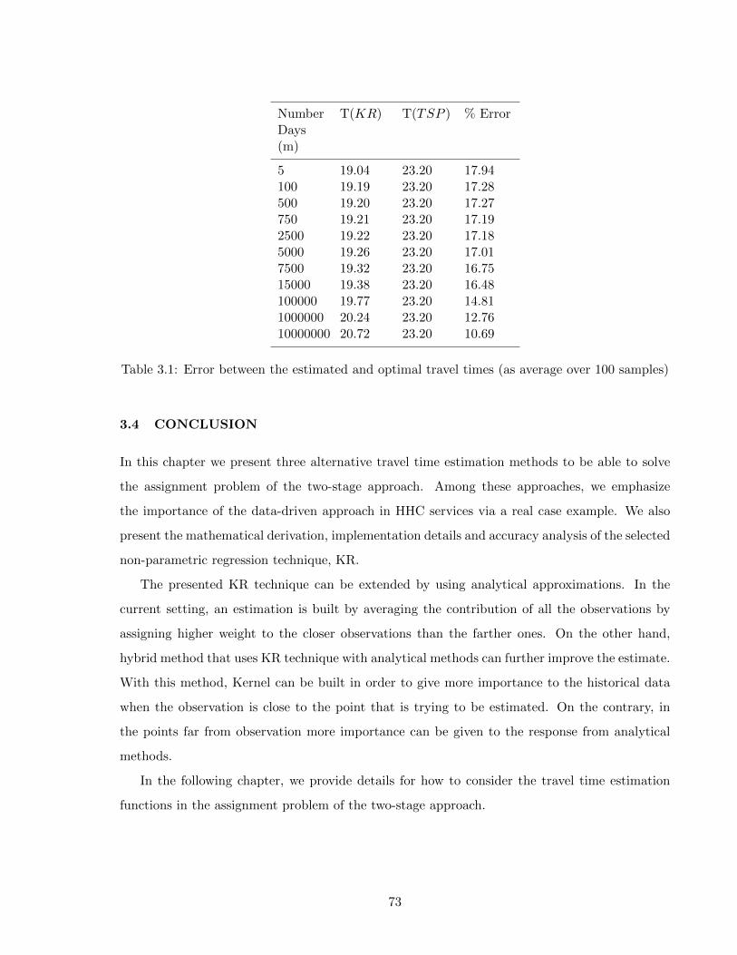
NumberDays(m)
T(KR) T(TSP ) % Error
5 19.04 23.20 17.94100 19.19 23.20 17.28500 19.20 23.20 17.27750 19.21 23.20 17.192500 19.22 23.20 17.185000 19.26 23.20 17.017500 19.32 23.20 16.7515000 19.38 23.20 16.48100000 19.77 23.20 14.811000000 20.24 23.20 12.7610000000 20.72 23.20 10.69
Table 3.1: Error between the estimated and optimal travel times (as average over 100 samples)
3.4 CONCLUSION
In this chapter we present three alternative travel time estimation methods to be able to solve
the assignment problem of the two-stage approach. Among these approaches, we emphasize
the importance of the data-driven approach in HHC services via a real case example. We also
present the mathematical derivation, implementation details and accuracy analysis of the selected
non-parametric regression technique, KR.
The presented KR technique can be extended by using analytical approximations. In the
current setting, an estimation is built by averaging the contribution of all the observations by
assigning higher weight to the closer observations than the farther ones. On the other hand,
hybrid method that uses KR technique with analytical methods can further improve the estimate.
With this method, Kernel can be built in order to give more importance to the historical data
when the observation is close to the point that is trying to be estimated. On the contrary, in
the points far from observation more importance can be given to the response from analytical
methods.
In the following chapter, we provide details for how to consider the travel time estimation
functions in the assignment problem of the two-stage approach.
73

Figure 3.1: Optimal vs Realized (executed) Operator Tour
74

Figure 3.2: Procedure for Implementing Kernel Technique
75
Chapter 4
SOLUTION APPROACHES
4.1 INTRODUCTION
In this chapter, we use two solution methods based on the standard CPLEX solver and Genetic
Algorithm (GA) to solve models presented in Chapter 2. The aim of this chapter is to present
the details of the considered solution methods especially the GA. The chapter is organized by
first presenting a general procedure for the GA and then, providing details for the developed
GAs. Finally, information related to embedding the travel time functions are given.
Although it is possible to use CPLEX to solve both the two-stage and simultaneous ap-
proaches, in some cases GA is preferred because of three main reasons. The first one is the
computational complexity encountered in the simultaneous approach, especially for large in-
stances. The second reason is that KR and OSAV functions are fitted to calculate directly the
total travel time of an operator (not on each patient separately) and considering this in a GA
method is much more easier rather than in a mathematical programming model. The last reason
is the non-linear property of the Kernel function.
Note that, in Chapter 5 results of the numerical experiment are provided and these results
are grouped in two parts (i.e. in Part III and Part IV). The first part is used to analyze the
performance of different travel time estimation methods on the two-stage approach whereas the
second part is based on the different skill management (i.e. hierarchical or independent skill
management) alternatives. Different models are considered in each part and they are solved with
either CPLEX solver or GA in the first part and only CPLEX solver is used in the second part.
Table 4.1 summarizes the considered solutions methods for each part and case explicitly.
To sum up, as presented in Table 4.1 while a GA is used for the simultaneous approach in
Part III of Chapter 5 and the two-stage approach using the KR and OSAV functions (i.e. in
76
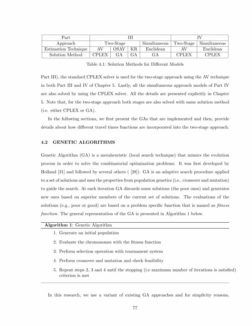
Part III IV
Approach Two-Stage Simultaneous Two-Stage Simultaneous
Estimation Technique AV OSAV KR Euclidean AV Euclidean
Solution Method CPLEX GA GA GA CPLEX CPLEX
Table 4.1: Solution Methods for Different Models
Part III), the standard CPLEX solver is used for the two-stage approach using the AV technique
in both Part III and IV of Chapter 5. Lastly, all the simultaneous approach models of Part IV
are also solved by using the CPLEX solver. All the details are presented explicitly in Chapter
5. Note that, for the two-stage approach both stages are also solved with same solution method
(i.e. either CPLEX or GA).
In the following sections, we first present the GAs that are implemented and then, provide
details about how different travel times functions are incorporated into the two-stage approach.
4.2 GENETIC ALGORITHMS
Genetic Algorithm (GA) is a metaheuristic (local search technique) that mimics the evolution
process in order to solve the combinatorial optimization problems. It was first developed by
Holland [31] and followed by several others ( [28]). GA is an adaptive search procedure applied
to a set of solutions and uses the properties from population genetics (i.e., crossover and mutation)
to guide the search. At each iteration GA discards some solutions (the poor ones) and generates
new ones based on superior members of the current set of solutions. The evaluations of the
solutions (e.g., poor or good) are based on a problem specific function that is named as fitness
function. The general representation of the GA is presented in Algorithm 1 below.
Algorithm 1: Genetic Algorithm
1. Generate an initial population
2. Evaluate the chromosomes with the fitness function
3. Perform selection operation with tournament system
4. Perform crossover and mutation and check feasibility
5. Repeat steps 2, 3 and 4 until the stopping (i.e maximum number of iterations is satisfied)criterion is met
In this research, we use a variant of existing GA approaches and for simplicity reasons,
77
we refer to it as GA as well. Different than the classical published GA works that deal with
the assignment and routing problems ( [42]), here we produce children from a single parent so
crossover operator transforms a single chromosome. Due to such a property, the GA procedure
turns out to be a random local search method where new solutions are derived from a current
solution by transformation, but without any neighborhood exploration. Since management of
populations solutions is similar to the classical GA, our approach can be considered as a variant
of the GA.
Since GA is applied for both the two-stage and simultaneous approaches, there exits differ-
ences between each GA. The following parts provide details on the first GA that is used to solve
the simultaneous approach (see Section 4.2.1), the second one is adopted for the assignment
problem of the two-stage approach (see Section 4.2.2), the last one is used to solve the routing
problem of the two stage approach (see Section 4.2.3).
Note that the presented GAs are only applied to the models with independent skill, multiple
planning periods and capacity constraints of operators. The models with hierarchical skills are
solved using the two-stage approach by only considering the AV technique. Thus, the corre-
sponding solutions are obtained with the CPLEX solver and no GA is developed neither for this
two-stage approach nor for the benchmark approach.
4.2.1 Simultaneous Approach
In this section we present each phase of the GA such as the encoding, fitness function evaluation,
population selection procedure, crossover and mutation operations, and the feasibility. Finally,
we also provide a performance analysis of the developed GA.
Encoding (Representation)
Each solution in GA is represented as a chromosome where in each chromosome, the visiting
sequences of each operator is identified with ones. In particular, for each chromosome, patients
and associated patterns are identified with numbers between 2 and N+1 for patients, 2 and P+1
for patterns. Figure 4.1 represents the chromosome for the visiting sequence with 3 operators
with 10 patients and 4 patterns (i.e. each gene is divided into two parts representing the id of
the patient and id of the assigned pattern (|patient|pattern|)).
78
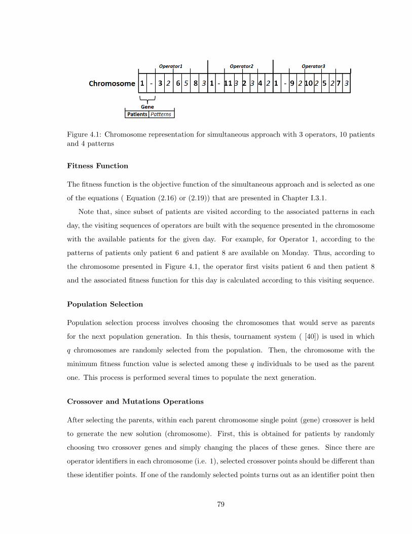
Figure 4.1: Chromosome representation for simultaneous approach with 3 operators, 10 patientsand 4 patterns
Fitness Function
The fitness function is the objective function of the simultaneous approach and is selected as one
of the equations ( Equation (2.16) or (2.19)) that are presented in Chapter I.3.1.
Note that, since subset of patients are visited according to the associated patterns in each
day, the visiting sequences of operators are built with the sequence presented in the chromosome
with the available patients for the given day. For example, for Operator 1, according to the
patterns of patients only patient 6 and patient 8 are available on Monday. Thus, according to
the chromosome presented in Figure 4.1, the operator first visits patient 6 and then patient 8
and the associated fitness function for this day is calculated according to this visiting sequence.
Population Selection
Population selection process involves choosing the chromosomes that would serve as parents
for the next population generation. In this thesis, tournament system ( [40]) is used in which
q chromosomes are randomly selected from the population. Then, the chromosome with the
minimum fitness function value is selected among these q individuals to be used as the parent
one. This process is performed several times to populate the next generation.
Crossover and Mutations Operations
After selecting the parents, within each parent chromosome single point (gene) crossover is held
to generate the new solution (chromosome). First, this is obtained for patients by randomly
choosing two crossover genes and simply changing the places of these genes. Since there are
operator identifiers in each chromosome (i.e. 1), selected crossover points should be different than
these identifier points. If one of the randomly selected points turns out as an identifier point then
79

the selection process is repeated until a patient point is found. This operation corresponds to
either changing the operator-patient match or keeping the match same and changing the visiting
sequence of the selected patients for an operator. For example, in Figure 4.1, if crossover is
held for the 2nd and 6th patients (corresponds to 3rd and 7th genes of the chromosome) then
in the new chromosome, patient 2 will be visited by Operator 1 and patient 6 will be visited
by Operator 2. As the next step, this crossover operation is also repeated for the patterns by
randomly choosing two points from the second part of each gene (i.e. first part of the gene is not
replaced thus, only associated patterns of patients are changed) without considering the gene
that corresponds to the operator identifier.
With the mutation operation two new solutions are generated by using a parent chromosome.
The first one is obtained by moving a gene randomly to another position in the chromosome (slide
the gene). For example, moving the second gene (i.e. patient 3 with pattern 2) to the last position
in Figure 4.1 where both the selected gene and the new position is chosen randomly. In the new
chromosome patient 3 is assigned to Operator 3 and will be visited according to the associated
pattern. The second mutation operation is the flipping where the order of the selected genes are
flipped. For example, 3rd and 8th genes are randomly chosen from the chromosome of Figure
4.1 and all genes in between are flipped. The new chromosome is presented in Figure 4.2. Here
the only concern is again the selected gene. Any selected gene should not contain the operator
identifier 1.
Figure 4.2: Chromosome representation after flipping the genes between 3th and 8th genes
Feasibility
Since each operator should have at least one assigned patient and each patient can only be as-
signed to a single operator, for each new chromosome generated by the crossover and mutation
operations, the feasibility should be checked. The structure of the population matrix (see chro-
mosome representation) always ensures the constraint where each patient can only be assigned
once. Thus, no extra effort is required for this constraint. Concerning the pattern feasibility,
80
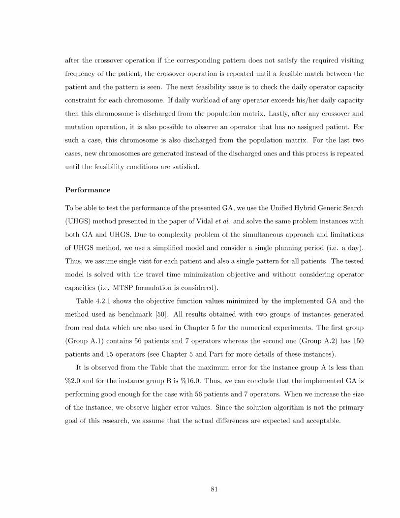
after the crossover operation if the corresponding pattern does not satisfy the required visiting
frequency of the patient, the crossover operation is repeated until a feasible match between the
patient and the pattern is seen. The next feasibility issue is to check the daily operator capacity
constraint for each chromosome. If daily workload of any operator exceeds his/her daily capacity
then this chromosome is discharged from the population matrix. Lastly, after any crossover and
mutation operation, it is also possible to observe an operator that has no assigned patient. For
such a case, this chromosome is also discharged from the population matrix. For the last two
cases, new chromosomes are generated instead of the discharged ones and this process is repeated
until the feasibility conditions are satisfied.
Performance
To be able to test the performance of the presented GA, we use the Unified Hybrid Generic Search
(UHGS) method presented in the paper of Vidal et al. and solve the same problem instances with
both GA and UHGS. Due to complexity problem of the simultaneous approach and limitations
of UHGS method, we use a simplified model and consider a single planning period (i.e. a day).
Thus, we assume single visit for each patient and also a single pattern for all patients. The tested
model is solved with the travel time minimization objective and without considering operator
capacities (i.e. MTSP formulation is considered).
Table 4.2.1 shows the objective function values minimized by the implemented GA and the
method used as benchmark [50]. All results obtained with two groups of instances generated
from real data which are also used in Chapter 5 for the numerical experiments. The first group
(Group A.1) contains 56 patients and 7 operators whereas the second one (Group A.2) has 150
patients and 15 operators (see Chapter 5 and Part for more details of these instances).
It is observed from the Table that the maximum error for the instance group A is less than
%2.0 and for the instance group B is %16.0. Thus, we can conclude that the implemented GA is
performing good enough for the case with 56 patients and 7 operators. When we increase the size
of the instance, we observe higher error values. Since the solution algorithm is not the primary
goal of this research, we assume that the actual differences are expected and acceptable.
81
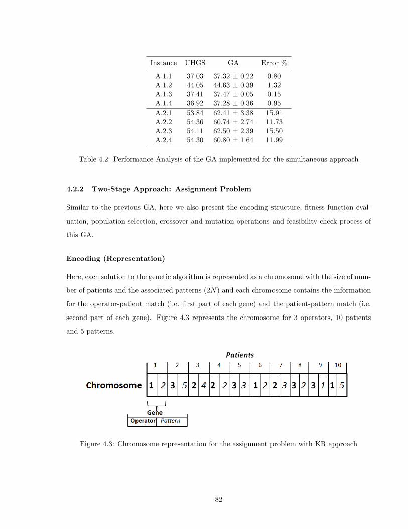
Instance UHGS GA Error %
A.1.1 37.03 37.32 ± 0.22 0.80A.1.2 44.05 44.63 ± 0.39 1.32A.1.3 37.41 37.47 ± 0.05 0.15A.1.4 36.92 37.28 ± 0.36 0.95
A.2.1 53.84 62.41 ± 3.38 15.91A.2.2 54.36 60.74 ± 2.74 11.73A.2.3 54.11 62.50 ± 2.39 15.50A.2.4 54.30 60.80 ± 1.64 11.99
Table 4.2: Performance Analysis of the GA implemented for the simultaneous approach
4.2.2 Two-Stage Approach: Assignment Problem
Similar to the previous GA, here we also present the encoding structure, fitness function eval-
uation, population selection, crossover and mutation operations and feasibility check process of
this GA.
Encoding (Representation)
Here, each solution to the genetic algorithm is represented as a chromosome with the size of num-
ber of patients and the associated patterns (2N) and each chromosome contains the information
for the operator-patient match (i.e. first part of each gene) and the patient-pattern match (i.e.
second part of each gene). Figure 4.3 represents the chromosome for 3 operators, 10 patients
and 5 patterns.
Figure 4.3: Chromosome representation for the assignment problem with KR approach
82
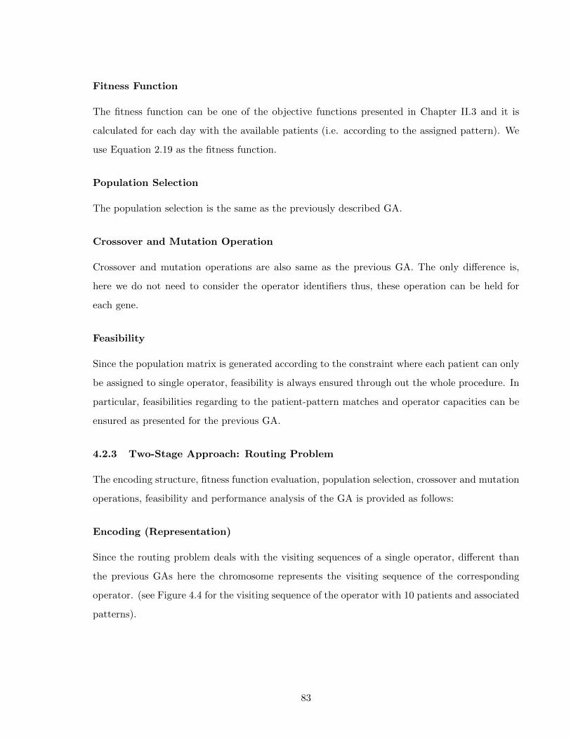
Fitness Function
The fitness function can be one of the objective functions presented in Chapter II.3 and it is
calculated for each day with the available patients (i.e. according to the assigned pattern). We
use Equation 2.19 as the fitness function.
Population Selection
The population selection is the same as the previously described GA.
Crossover and Mutation Operation
Crossover and mutation operations are also same as the previous GA. The only difference is,
here we do not need to consider the operator identifiers thus, these operation can be held for
each gene.
Feasibility
Since the population matrix is generated according to the constraint where each patient can only
be assigned to single operator, feasibility is always ensured through out the whole procedure. In
particular, feasibilities regarding to the patient-pattern matches and operator capacities can be
ensured as presented for the previous GA.
4.2.3 Two-Stage Approach: Routing Problem
The encoding structure, fitness function evaluation, population selection, crossover and mutation
operations, feasibility and performance analysis of the GA is provided as follows:
Encoding (Representation)
Since the routing problem deals with the visiting sequences of a single operator, different than
the previous GAs here the chromosome represents the visiting sequence of the corresponding
operator. (see Figure 4.4 for the visiting sequence of the operator with 10 patients and associated
patterns).
83
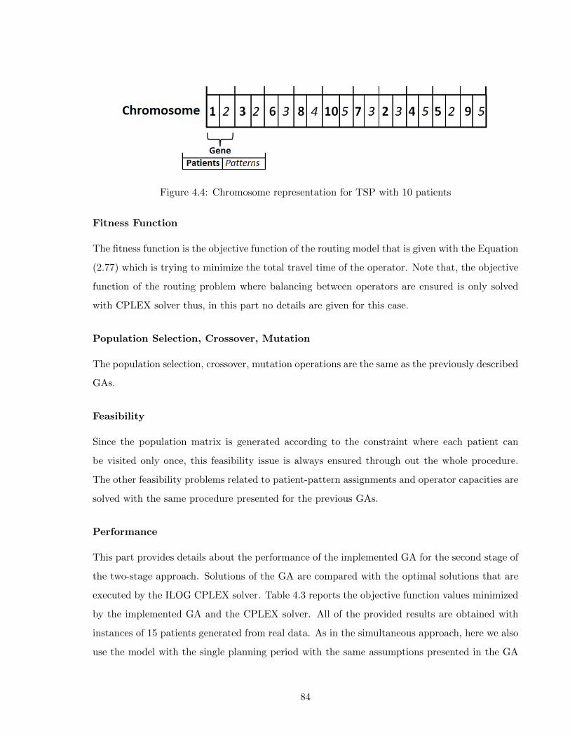
Figure 4.4: Chromosome representation for TSP with 10 patients
Fitness Function
The fitness function is the objective function of the routing model that is given with the Equation
(2.77) which is trying to minimize the total travel time of the operator. Note that, the objective
function of the routing problem where balancing between operators are ensured is only solved
with CPLEX solver thus, in this part no details are given for this case.
Population Selection, Crossover, Mutation
The population selection, crossover, mutation operations are the same as the previously described
GAs.
Feasibility
Since the population matrix is generated according to the constraint where each patient can
be visited only once, this feasibility issue is always ensured through out the whole procedure.
The other feasibility problems related to patient-pattern assignments and operator capacities are
solved with the same procedure presented for the previous GAs.
Performance
This part provides details about the performance of the implemented GA for the second stage of
the two-stage approach. Solutions of the GA are compared with the optimal solutions that are
executed by the ILOG CPLEX solver. Table 4.3 reports the objective function values minimized
by the implemented GA and the CPLEX solver. All of the provided results are obtained with
instances of 15 patients generated from real data. As in the simultaneous approach, here we also
use the model with the single planning period with the same assumptions presented in the GA
84

for the simultaneous approach (i.e. basic TSP model is considered). It is possible to observe that
the GA for the TSP always provided the optimal solution.
Instance CPLEX GA Error %
1 333.94 333.94 0.02 327.66 327.66 0.03 341.43 341.43 0.04 321.21 321.21 0.0
Table 4.3: Performance Analysis of the GA implemented for the routing problem of the two-stageapproach
The following section provides details about how the travel time estimation functions that
are presented in Chapter 3 can be implemented into the two-stage approach.
4.3 HOW TO CALL THE TRAVEL TIME FUNCTION
Regarding the AV approach, since the average travel times are calculated over all patients before
solving the assignment problem, the incorporation of calculated estimations can be accomplished
by using these values as patient related input parameters. Then putting them into the relevant
equation (e.g. Equations (2.46)) provides the total travel time estimation of each operator.
With respect to KR and OSAV estimations, because the functions are fitted to calculate
directly the total travel time of an operator, the incorporation of these estimations into the
assignment problem is more difficult than the AV approach. As mentioned before, GA is adopted
to be able to cope with such complexities. Indeed, it is not difficult to embed these functions into
this heuristic approach since in each iteration of the GA, the assignment list of each operator is
known. Thus, direct computation of total travel times for each operator can be completed using
either the generated KR (each operator has its own KR function based on his learning) or OSAV
functions. Then, the algorithm can proceed for the next step where the fitness value is obtained.
4.4 CONCLUSION
In this chapter, we present the solution methods used in order to analyze the performance of the
models proposed for two-stage approach (cf. Part II of Chapter 2 ). Note that, in this thesis,
our objective is to assess the performance of the simultaneous and two-stage approaches (i.e. in
85

terms of objective function and total travel time of operators). In other words, the performances
of the presented GAs are not the main interest since we are not trying to contribute to the VRP
literature, rather we try to develop new decision tools for the assignment and routing problems
of the HHC literature. Hence, in the following chapter, we use these GAs to solve and present
the results of the two-stage approach using KR and OSAV techniques. On the other hand, the
commercial CPLEX solver is used to obtain the solutions of the models with AV approach.
In addition to the developed GAs, another proper approach to solve the two-stage models
with KR and OSAV functions can be the enumeration of all possible assignment combinations
for all operators and the estimation of the related travel times using these functions. These two
steps can be completed off-line, i.e., before solving the assignment problem and the corresponding
values can be evaluated with the use of a exact method like Column Generation (CG). However,
in this thesis, we only implement the GA as a solution method for the two-stage approach with
KR and OSAV.
86
Chapter 5
COMPUTATIONAL STUDY
5.1 INTRODUCTION
In this chapter, we present results of the numerical experiments that analyze the performance of
models proposed for the two-stage approach with respect to the simultaneous approach.
Results are grouped in two parts where Part III assesses the performance of different travel
time estimation methods on the two-stage approach and Part IV assesses the impact of alterna-
tives in terms of operator skill management. In each part different models and different solution
techniques are used to analyze the performance of some specific cases considered. More specif-
ically, the first part mainly focuses on the performance of the travel time estimation methods.
Thus, different travel time estimation methods are used for different variants of the two-stage
model. Since the nature of operator skills is not the focus, we assume that operators have iden-
tical skills. The focus of the second part is the skill management issue. Both two-stage and
simultaneous approach models are tested with independently and hierarchically managed oper-
ator skills by considering the AV technique as the travel time estimation method (see Table 5.1
for the summary).
Part III IV
FocusPerformance of Travel Time Skill Management
Estimation Methods Alternatives
Models I,III,IV,V I,II,III,IV,V
Travel Time Estimation Method AV,OSAV,KR and Euclidean AV and Euclidean
Operator Skills Single and Identical 2 Skill Levels and Not Identical
Planning Period Single and Multiple Multiple
Solution Approach GA and CPLEX CPLEX
Table 5.1: Summary for the Experimentations
87

Each part starts by presenting the design of experiments carried and then, provides infor-
mation related to the experimental settings used for the instances as well as solution methods.
Finally, several numerical results are analyzed in details.
Note that all instances used in this work are obtained from real data provided by an Italian
HHC provider for which patient locations, patient demands and standard service times for the
past four years are available.
88

Part III
ASSESSING THE PERFORMANCE OF TRAVEL TIME ESTIMATION
METHODS USED IN THE TWO-STAGE PLANNING APPROACH
89
III.1 INTRODUCTION
The aim of this part is to analyze the performance of each travel time estimation method used in
the two-stage approach (i.e. the AV, OSAV and KR methods) in comparison to models developed
for the simultaneous approach.
All alternative modeling scenarios (excluding Model II) that are proposed for the two-stage
approach (cf. Figure II.1 in Chapter 2) are tested on several instances. Numerical studies
are developed for various settings such as single or multiple planning periods, with or without
operator capacity restrictions.
Section III.2, provides details on the design of experiments . Then, in Section III.3, we present
parameters related to the instances and solution methods considered. Lastly, in Section IV.4,
numerical results are provided with a detailed analysis.
Note that in addition to modeling scenarios presented for the two-stage approach (cf. Figure
II.1) the model referring to the simultaneous approach is called Model V in the rest of this thesis.
III.2 DESIGN OF EXPERIMENTS
Two groups of experiments are considered: Group A experiments that are based on a single
planning period and Group B that considers multiple planning periods. In Group A, Model
I (two-stage model) and Model V (simultaneous model) are used to test the performances of
different travel time estimation methods (i.e. AV, OSAV and KR) based on the simplest model
setting that assumes a single day of planning and released operator capacities.
Group B experiments focus more on the performance of the two-stage approach using the
KR technique. In order to do this, in addition to the KR technique, we also consider a second
travel time estimation technique (either AV or OSAV) that yields the best performance in the
experiments carried in Group A. Different than Group A experiment, the considered modeling
assumptions are multiple planning periods assumption and restricted operator capacities. This
enables to further analyze the performances of the KR technique and the two-stage approach
under more complex conditions.
In both experiment groups, we assume that all operators are identical in terms of skill qualifi-
cations and daily working capacities. Furthermore, all models are solved to balance the trade-off
between operators’ workload balancing and operators’ total travel times (i.e. Equation 2.19). In
90
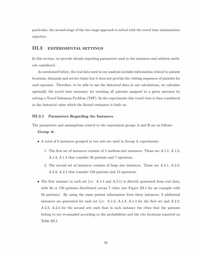
particular, the second-stage of the two stage approach is solved with the travel time minimization
objective.
III.3 EXPERIMENTAL SETTINGS
In this section, we provide details regarding parameters used in the instances and solution meth-
ods considered.
As mentioned before, the real data used in our analysis includes information related to patient
locations, demands and service times but it does not provide the visiting sequences of patients for
each operator. Therefore, to be able to use the historical data in our calculations, we calculate
optimally the travel time necessary for reaching all patients assigned to a given operator by
solving a Travel Salesman Problem (TSP). In the experiments this travel time is then considered
as the historical value which the Kernel estimator is built on.
III.3.1 Parameters Regarding the Instances
The parameters and assumptions related to the experiment groups A and B are as follows:
Group A:
• A total of 8 instances grouped in two sets are used in Group A experiments.
1. The first set of instances consists of 4 medium-size instances. Those are A.1.1, A.1.2,
A.1.3, A.1.4 that consider 56 patients and 7 operators.
2. The second set of instances consists of large size instances. Those are A.2.1, A.2.2,
A.2.3, A.2.4 that consider 150 patients and 15 operators.
• The first instance in each set (i.e. A.1.1 and A.2.1) is directly generated from real data,
with 56 or 150 patients distributed across 7 cities (see Figure III.1 for an example with
56 patients). By using the same patient information from these instances, 3 additional
instances are generated for each set (i.e. A.1.2, A.1.3, A.1.4 for the first set and A.2.2,
A.2.3, A.2.4 for the second set) such that in each instance the cities that the patients
belong to are re-sampled according to the probabilities and the city locations reported on
Table III.1.
91
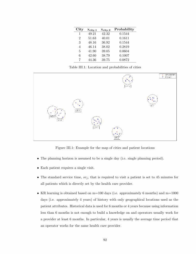
City xcity,1 xcity,2 Probability
1 49.21 42.32 0.15442 51.63 40.01 0.16113 48.16 36.92 0.15444 46.14 38.02 0.28195 41.90 39.05 0.06046 42.60 38.79 0.10077 44.36 39.75 0.0872
Table III.1: Location and probabilities of cities
Figure III.1: Example for the map of cities and patient locations
• The planning horizon is assumed to be a single day (i.e. single planning period).
• Each patient requires a single visit.
• The standard service time, svj , that is required to visit a patient is set to 45 minutes for
all patients which is directly set by the health care provider.
• KR learning is obtained based on m=100 days (i.e. approximately 6 months) and m=1000
days (i.e. approximately 4 years) of history with only geographical locations used as the
patient attributes. Historical data is used for 6 months or 4 years because using information
less than 6 months is not enough to build a knowledge on and operators usually work for
a provider at least 6 months. In particular, 4 years is usually the average time period that
an operator works for the same health care provider.
92
• The trade-off parameter γ is assumed to be 1/100 for medium-sized and 1/750 for large-
sized instances. In addition to these values, in Section III.4.2.2, we also provide a sensitivity
analysis to show that for several other γ values the solutions are consistent according to
the nature of the trade-off function (i.e. increasing γ results in higher total travel time
values and lower balance between operators).
Group B:
• A total of 10 instances are considered in Group B. All instances are medium-size instances
that use 44 to 56 patients and 4 operators as reported in Table III.2.
• Different than Group A instances, all instance are directly generated from real data.
• Operators are allowed to work 400, 350, 300 and 300 minutes per day respectively and
these values are directly obtained from the data given by the health care provider.
• The planning horizon consists of 6 days (i.e. multiple planning periods).
• Each patient requires 1 to 4 visits in total during the planning period of 6 days. The total
number of visits required among all patients is provided in column 3 of Table III.2.
• Remind that a pattern is a priori given schedule for a given set of visits (i.e. in total 2
visits on Tuesday and Friday etc.) and several patterns are usually defined to satisfy the
requirements of all patients. In this work, patterns for care plan decision are generated
with the flow based pattern policy given in the work of Cappanera and Scutella [17] for
each instance.
• The standard service time, svj , that is required to visit a patient is set to 45 minutes for
all patients.
• KR learning is obtained based on m=100 and m=1000 days of history with only geograph-
ical locations qs in the Group A instances.
• Several values between 0 and ∞ are assumed for the trade-off parameter γ to be able
to analyze the effect of workload balancing on the total travel times and vice versa. All
these values are specified explicitly in Section III.4.2. In particular, in Section III.4.2.4, a
sensitivity analysis is also done for different γ values as we do for the Group A instances.
93
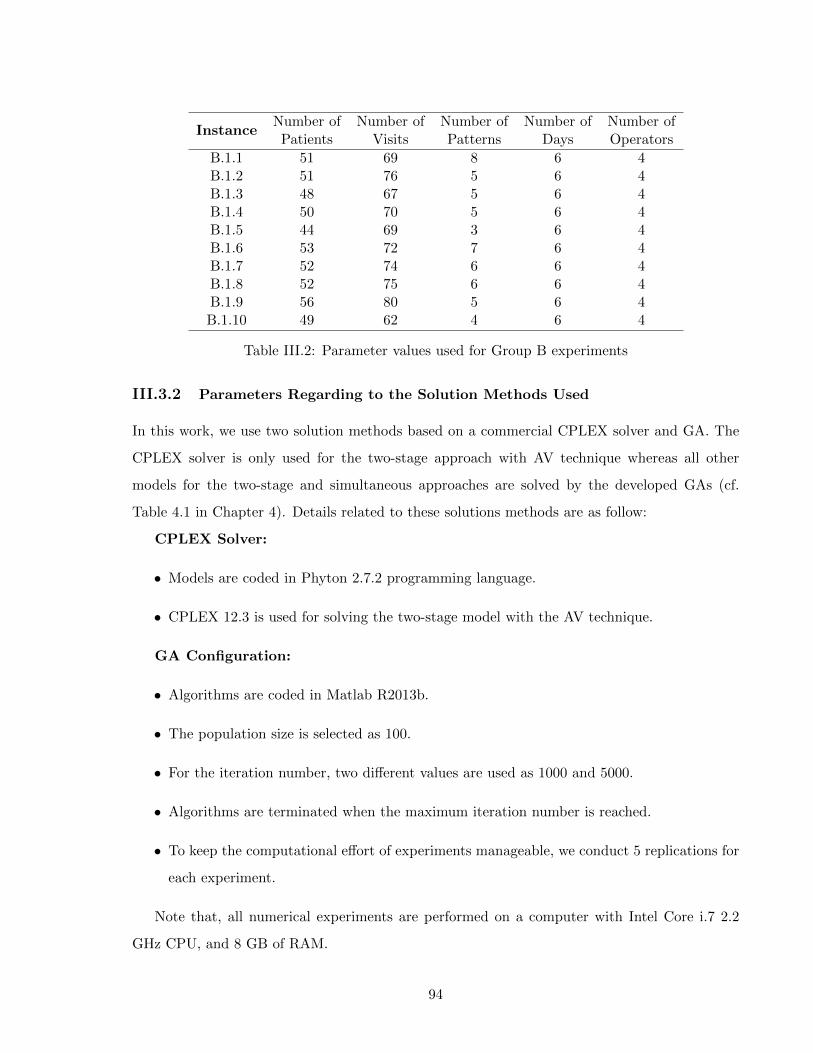
InstanceNumber of Number of Number of Number of Number ofPatients Visits Patterns Days Operators
B.1.1 51 69 8 6 4B.1.2 51 76 5 6 4B.1.3 48 67 5 6 4B.1.4 50 70 5 6 4B.1.5 44 69 3 6 4B.1.6 53 72 7 6 4B.1.7 52 74 6 6 4B.1.8 52 75 6 6 4B.1.9 56 80 5 6 4B.1.10 49 62 4 6 4
Table III.2: Parameter values used for Group B experiments
III.3.2 Parameters Regarding to the Solution Methods Used
In this work, we use two solution methods based on a commercial CPLEX solver and GA. The
CPLEX solver is only used for the two-stage approach with AV technique whereas all other
models for the two-stage and simultaneous approaches are solved by the developed GAs (cf.
Table 4.1 in Chapter 4). Details related to these solutions methods are as follow:
CPLEX Solver:
• Models are coded in Phyton 2.7.2 programming language.
• CPLEX 12.3 is used for solving the two-stage model with the AV technique.
GA Configuration:
• Algorithms are coded in Matlab R2013b.
• The population size is selected as 100.
• For the iteration number, two different values are used as 1000 and 5000.
• Algorithms are terminated when the maximum iteration number is reached.
• To keep the computational effort of experiments manageable, we conduct 5 replications for
each experiment.
Note that, all numerical experiments are performed on a computer with Intel Core i.7 2.2
GHz CPU, and 8 GB of RAM.
94
III.4 NUMERICAL RESULTS
In this section, the proposed two-stage approach is compared to the simultaneous approach using
Group A and B instances. Section III.4.1 presents the performance indicators used to analyze
results. Then, in Section III.4.2 numerical results for the simple setting with Model I and Model
V are provided (i.e single period and no restriction on operator capacity) by using the instances
from Group A. The performances of KR, AV and OSAV methods in the two-stage approach
are evaluated. As the next step, we extend the numerical analysis to the cases where multiple
planning periods and operator capacities are considered. Results are developed for Group B.1
instances. Hence, Model III, Model IV and Model V are used to analyze the performance of the
two-stage approach with KR technique and the operator specific travel time estimation method
OSAV. Since we show that the OSAV method outperforms the AV method, the AV technique is
not included in further analysis. Lastly, sensitivity analysis is also carried out for both Group A
and B instances.
III.4.1 Performance Indicators
Three indicators are used to assess the performance of each model analyzed.
The total travel time of all operators obtained in the two-stage approach with the AV, OSAV
and KR methods are represented by T(AV ), T(OSAV ) and T(KR), respectively, and the work-
load balance value between the maximally and minimally utilized operators are represented by
B(AV ), B(OSAV ) and B(KR), respectively. Similarly, the total travel time in the simultaneous
approach is denoted by T(V RP ), and the balancing value is denoted by B(V RP ). Because the
models are solved to balance the trade-off between operators’ workload and total travel times,
the corresponding value is denoted as Obj., which equals to h(.) + γT (.) where h(.) corresponds
to the maximum operator utilization level.
T(AV ), T(OSAV ) and T(KR) values are obtained by solving several (as the number of
operators) independent TSP models (i.e. the objective function is travel time minimization),
with the outputs obtained from the assignment stage and summing up the results obtained from
each TSP model across the seven operators. T(V RP ) values are directly calculated from the
corresponding simultaneous model as the sum of each operator’s route time.
Because we use a genetic algorithm for both the two-stage approach with the KR and OSAV
techniques as well as the simultaneous approach, T(.) and B(.) values are obtained as the average
95
values from 5 replications of the algorithms, and corresponding Obj. values are calculated based
on a %95 confidence interval. Moreover, the results of the two-stage approach using the AV
technique are obtained with the ILOG Cplex solver for both stages thus, we do not provide a
confidence interval for the two-stage approach using the AV technique.
III.4.2 Results
Section III.4.2.1 presents the results associated with Group A instances that compare Model I
to Model V where AV, OSAV and KR methods are used as travel time estimators in the first
stage of Model I. Then, Section III.4.2.3 provides other results with Group B instances for Model
III, Model IV and Model V. In this case, only OSAV and KR methods are used as travel time
estimator within the Model III and Model IV. In Section III.4.2.2 and Section III.4.2.4, results
for the sensitivity analysis are presented as well.
III.4.2.1 Results Pertaining to Group A Instances
In this section, we analyze the performance of the KR technique in comparison to AV and OSAV
techniques. Then, we conduct a sensitivity analysis based on different historical data (i.e. m)
values.
Results for Group A.1 Instances:
As Table III.3 indicates, there are two types of results related to the two-stage approach.
One of them is referred as the Non Uniformized two-stage KR approach (cf. columns 2,3,4) and
the other one is called the Uniformized (Unif.) two-stage KR approach (cf. columns 5,6,7). For
the second case, we consider the uniformization of the input data used in the KR function. For
example, a patient can occupy the first position (i.e., the rank in the input matrix) in a planning
horizon and can be considered in the third position in the following horizon. Thus, if we do
not uniformize the input data, the KR function might not recognize that these patients refer
to the same patient and may spend unnecessary time providing a better estimate by building
a structure across all the dimensions (as the number of patients). To avoid this computation,
we use a simple ordering technique for the input data that sorts patients according to their
geographical locations (based on X and Y coordinates). This technique calculates an Order
Value (OV) for each patient, OV = X + aY (a is a positive integer), and generates the input
data by sorting patients in descending order of their OV values.
96
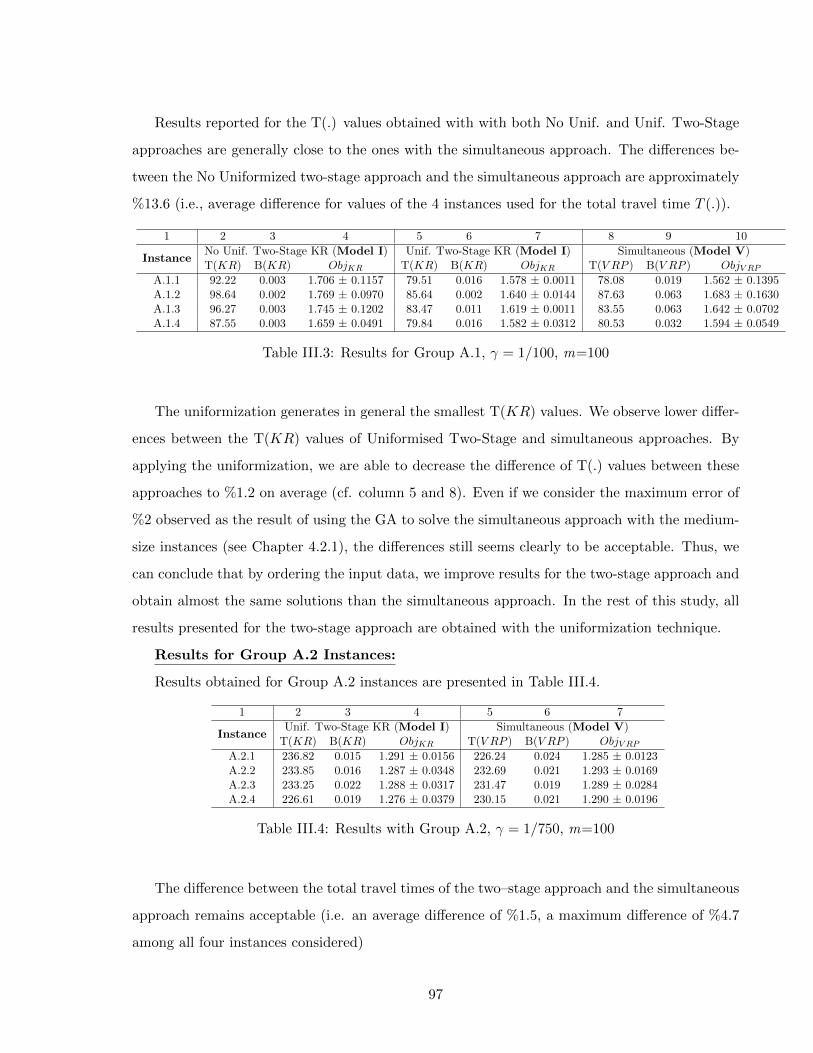
Results reported for the T(.) values obtained with with both No Unif. and Unif. Two-Stage
approaches are generally close to the ones with the simultaneous approach. The differences be-
tween the No Uniformized two-stage approach and the simultaneous approach are approximately
%13.6 (i.e., average difference for values of the 4 instances used for the total travel time T (.)).
1 2 3 4 5 6 7 8 9 10
InstanceNo Unif. Two-Stage KR (Model I) Unif. Two-Stage KR (Model I) Simultaneous (Model V)T(KR) B(KR) ObjKR T(KR) B(KR) ObjKR T(V RP ) B(V RP ) ObjV RP
A.1.1 92.22 0.003 1.706 ± 0.1157 79.51 0.016 1.578 ± 0.0011 78.08 0.019 1.562 ± 0.1395A.1.2 98.64 0.002 1.769 ± 0.0970 85.64 0.002 1.640 ± 0.0144 87.63 0.063 1.683 ± 0.1630A.1.3 96.27 0.003 1.745 ± 0.1202 83.47 0.011 1.619 ± 0.0011 83.55 0.063 1.642 ± 0.0702A.1.4 87.55 0.003 1.659 ± 0.0491 79.84 0.016 1.582 ± 0.0312 80.53 0.032 1.594 ± 0.0549
Table III.3: Results for Group A.1, γ = 1/100, m=100
The uniformization generates in general the smallest T(KR) values. We observe lower differ-
ences between the T(KR) values of Uniformised Two-Stage and simultaneous approaches. By
applying the uniformization, we are able to decrease the difference of T(.) values between these
approaches to %1.2 on average (cf. column 5 and 8). Even if we consider the maximum error of
%2 observed as the result of using the GA to solve the simultaneous approach with the medium-
size instances (see Chapter 4.2.1), the differences still seems clearly to be acceptable. Thus, we
can conclude that by ordering the input data, we improve results for the two-stage approach and
obtain almost the same solutions than the simultaneous approach. In the rest of this study, all
results presented for the two-stage approach are obtained with the uniformization technique.
Results for Group A.2 Instances:
Results obtained for Group A.2 instances are presented in Table III.4.
1 2 3 4 5 6 7
InstanceUnif. Two-Stage KR (Model I) Simultaneous (Model V)
T(KR) B(KR) ObjKR T(V RP ) B(V RP ) ObjV RP
A.2.1 236.82 0.015 1.291 ± 0.0156 226.24 0.024 1.285 ± 0.0123A.2.2 233.85 0.016 1.287 ± 0.0348 232.69 0.021 1.293 ± 0.0169A.2.3 233.25 0.022 1.288 ± 0.0317 231.47 0.019 1.289 ± 0.0284A.2.4 226.61 0.019 1.276 ± 0.0379 230.15 0.021 1.290 ± 0.0196
Table III.4: Results with Group A.2, γ = 1/750, m=100
The difference between the total travel times of the two–stage approach and the simultaneous
approach remains acceptable (i.e. an average difference of %1.5, a maximum difference of %4.7
among all four instances considered)
97
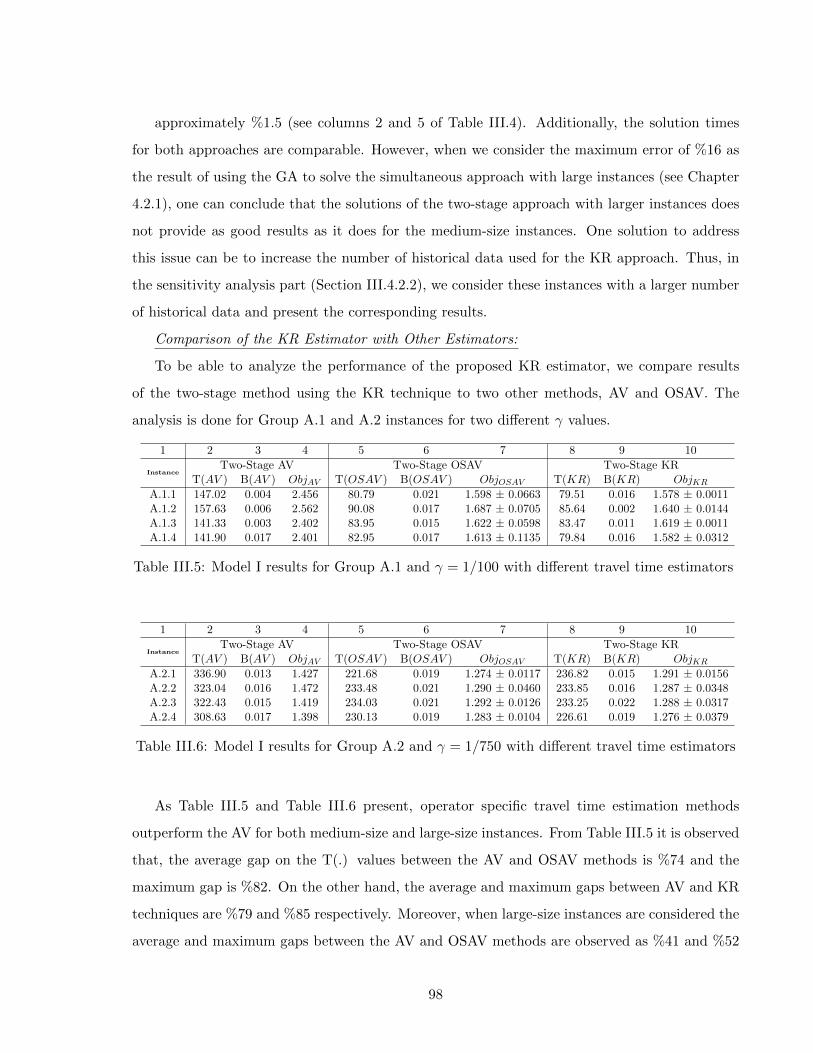
approximately %1.5 (see columns 2 and 5 of Table III.4). Additionally, the solution times
for both approaches are comparable. However, when we consider the maximum error of %16 as
the result of using the GA to solve the simultaneous approach with large instances (see Chapter
4.2.1), one can conclude that the solutions of the two-stage approach with larger instances does
not provide as good results as it does for the medium-size instances. One solution to address
this issue can be to increase the number of historical data used for the KR approach. Thus, in
the sensitivity analysis part (Section III.4.2.2), we consider these instances with a larger number
of historical data and present the corresponding results.
Comparison of the KR Estimator with Other Estimators:
To be able to analyze the performance of the proposed KR estimator, we compare results
of the two-stage method using the KR technique to two other methods, AV and OSAV. The
analysis is done for Group A.1 and A.2 instances for two different γ values.
1 2 3 4 5 6 7 8 9 10
InstanceTwo-Stage AV Two-Stage OSAV Two-Stage KR
T(AV ) B(AV ) ObjAV T(OSAV ) B(OSAV ) ObjOSAV T(KR) B(KR) ObjKR
A.1.1 147.02 0.004 2.456 80.79 0.021 1.598 ± 0.0663 79.51 0.016 1.578 ± 0.0011A.1.2 157.63 0.006 2.562 90.08 0.017 1.687 ± 0.0705 85.64 0.002 1.640 ± 0.0144A.1.3 141.33 0.003 2.402 83.95 0.015 1.622 ± 0.0598 83.47 0.011 1.619 ± 0.0011A.1.4 141.90 0.017 2.401 82.95 0.017 1.613 ± 0.1135 79.84 0.016 1.582 ± 0.0312
Table III.5: Model I results for Group A.1 and γ = 1/100 with different travel time estimators
1 2 3 4 5 6 7 8 9 10
InstanceTwo-Stage AV Two-Stage OSAV Two-Stage KR
T(AV ) B(AV ) ObjAV T(OSAV ) B(OSAV ) ObjOSAV T(KR) B(KR) ObjKR
A.2.1 336.90 0.013 1.427 221.68 0.019 1.274 ± 0.0117 236.82 0.015 1.291 ± 0.0156A.2.2 323.04 0.016 1.472 233.48 0.021 1.290 ± 0.0460 233.85 0.016 1.287 ± 0.0348A.2.3 322.43 0.015 1.419 234.03 0.021 1.292 ± 0.0126 233.25 0.022 1.288 ± 0.0317A.2.4 308.63 0.017 1.398 230.13 0.019 1.283 ± 0.0104 226.61 0.019 1.276 ± 0.0379
Table III.6: Model I results for Group A.2 and γ = 1/750 with different travel time estimators
As Table III.5 and Table III.6 present, operator specific travel time estimation methods
outperform the AV for both medium-size and large-size instances. From Table III.5 it is observed
that, the average gap on the T(.) values between the AV and OSAV methods is %74 and the
maximum gap is %82. On the other hand, the average and maximum gaps between AV and KR
techniques are %79 and %85 respectively. Moreover, when large-size instances are considered the
average and maximum gaps between the AV and OSAV methods are observed as %41 and %52
98
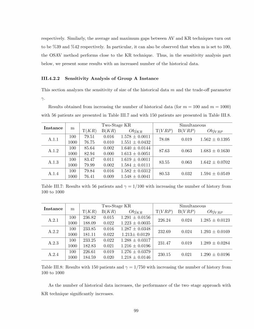
respectively. Similarly, the average and maximum gaps between AV and KR techniques turn out
to be %39 and %42 respectively. In particular, it can also be observed that when m is set to 100,
the OSAV method performs close to the KR technique. Thus, in the sensitivity analysis part
below, we present some results with an increased number of the historical data.
III.4.2.2 Sensitivity Analysis of Group A Instance
This section analyzes the sensitivity of size of the historical data m and the trade-off parameter
γ.
Results obtained from increasing the number of historical data (for m = 100 and m = 1000)
with 56 patients are presented in Table III.7 and with 150 patients are presented in Table III.8.
Instance mTwo-Stage KR Simultaneous
T(KR) B(KR) ObjKR T(V RP ) B(V RP ) ObjV RP
A.1.1100 79.51 0.016 1.578 ± 0.0011
78.08 0.019 1.562 ± 0.13951000 76.75 0.010 1.551 ± 0.0432
A.1.2100 85.64 0.002 1.640 ± 0.0144
87.63 0.063 1.683 ± 0.16301000 82.94 0.000 1.613 ± 0.0051
A.1.3100 83.47 0.011 1.619 ± 0.0011
83.55 0.063 1.642 ± 0.07021000 79.99 0.002 1.584 ± 0.0111
A.1.4100 79.84 0.016 1.582 ± 0.0312
80.53 0.032 1.594 ± 0.05491000 76.41 0.009 1.548 ± 0.0041
Table III.7: Results with 56 patients and γ = 1/100 with increasing the number of history from100 to 1000
Instance mTwo-Stage KR Simultaneous
T(KR) B(KR) ObjKR T(V RP ) B(V RP ) ObjV RP
A.2.1100 236.82 0.015 1.291 ± 0.0156
226.24 0.024 1.285 ± 0.01231000 188.09 0.022 1.223 ± 0.0035
A.2.2100 233.85 0.016 1.287 ± 0.0348
232.69 0.024 1.293 ± 0.01691000 181.11 0.022 1.213± 0.0129
A.2.3100 233.25 0.022 1.288 ± 0.0317
231.47 0.019 1.289 ± 0.02841000 182.83 0.021 1.216 ± 0.0196
A.2.4100 226.61 0.019 1.276 ± 0.0379
230.15 0.021 1.290 ± 0.01961000 184.59 0.020 1.218 ± 0.0146
Table III.8: Results with 150 patients and γ = 1/750 with increasing the number of history from100 to 1000
As the number of historical data increases, the performance of the two–stage approach with
KR technique significantly increases.
99

When the T(.) values of KR solutions from Tables III.7 and III.8 are compared with solutions
of the OSAV method from Table III.5 and Table III.6, one can remark that when the number of
historical days is increased to 1000, the KR technique starts to perform much more better than
the OSAV approach.
In particular, in the previous analysis, we observe that for large-size instances with m=100,
the results of KR approach do not seem to be as good as the ones of the medium-sized instances.
However, when we compare the solutions of the large-sized instances of the KR approach with
m=1000 (cf. Table III.8) with the solutions of the simultaneous approach ( cf. Table III.4) by
also considering the GA error of %16, we can conclude that with an enough number of historical
points, the two-stage approach with KR method presents similar solutions in comparison to the
simultaneous approach even for large instances.
For simplicity, all results presented so far are obtained by using two trade-off values, γ = 1/100
(i.e. Group A.1 instances) and γ = 1/750 (i.e. Group A.2 instances). Two different γ values are
chosen for each group since number of patients and operators are different as well. To be able
to show that the two-stage approach using KR estimation (i.e. OSAV performs similar as well,
see the sensitivity analysis in Section III.4.2.4) is also consistent with other penalty values, we
plot Figure III.2 using one of the medium-size instances. With this figure, we show the trade-off
between the workload balancing and total travel times of operators for decreasing values of the
trade-off term; results refer to the assignment phase of the two-stage process. As expected, it is
evident that when we decrease the trade-off value, the effect of the total travel time decreases
while better workload balancing is ensured. Thus, the KR predictor seems to correctly guide the
assignment problem in different situations.
In the following part, we extend our analysis with Group B instances to analyze the perfor-
mance of the two-stage approach with KR under more complex conditions.
III.4.2.3 Results with Group B Instances
We consider a single set of 10 instances to analyze the models with multiple planning periods
and operator capacities. Instances consist of 44 to 56 patients and 4 operators as presented on
Table III.2.
We start our analysis with a single instance (i.e. Instance B.1.1) and we consider 6 trade-off
values, γ, between zero and infinity. Then, for simplicity, we restrict our computations with two
100
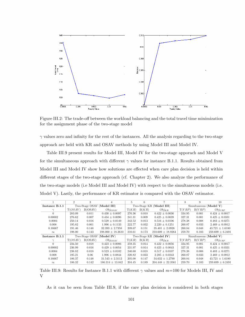
Figure III.2: The trade-off between the workload balancing and the total travel time minimizationfor the assignment phase of the two-stage model
γ values zero and infinity for the rest of the instances. All the analysis regarding to the two-stage
approach are held with KR and OSAV methods by using Model III and Model IV.
Table III.9 present results for Model III, Model IV for the two-stage apporach and Model V
for the simultaneous approach with different γ values for instance B.1.1. Results obtained from
Model III and Model IV show how solutions are effected when care plan decision is held within
different stages of the two-stage approach (cf. Chapter 2). We also analyze the performance of
the two-stage models (i.e Model III and Model IV) with respect to the simultaneous models (i.e.
Model V). Lastly, the performance of KR estimator is compared with the OSAV estimator.
1 2 3 4 5 6 7 8 9 10
Instance B.1.1 Two-Stage OSAV (Model III) Two-Stage KR (Model III) Simultaneous (Model V)γ T(OSAV ) B(OSAV) ObjOSAV T(KR) B(KR) ObjKR T(V RP ) B(V RP ) ObjV RP
0 283.09 0.011 0.430 ± 0.0097 276.36 0.010 0.422 ± 0.0036 334.95 0.001 0.424 ± 0.00170.00002 276.62 0.007 0.434 ± 0.0096 241.31 0.009 0.425 ± 0.0039 327.31 0.001 0.425 ± 0.03310.0004 250.14 0.016 0.529 ± 0.0149 242.52 0.013 0.516 ± 0.0106 278.38 0.008 0.483 ± 0.02710.008 195.82 0.061 1.996 ± 0.1133 222.77 0.032 2.220 ± 0.1251 260.87 0.033 2.469 ± 0.0912
0.16667 191.46 0.148 32.393 ± 2.7358 209.67 0.151 35.401 ± 2.0926 260.84 0.048 43.721 ± 1.6180∞ 198.00 0.143 198.000 ± 18.2610 210.61 0.173 210.609 ± 18.9264 259.70 0.103 259.699 ± 6.2491
Instance B.1.1 Two-Stage OSAV (Model IV) Two-Stage KR (Model IV) Simultaneous (Model V)γ T(OSAV ) B(OSAV) ObjOSAV T(KR) B(KR) ObjKR T(V RP ) B(V RP ) ObjV RP
0 234.50 0.018 0.423 ± 0.0086 259.35 0.014 0.422 ± 0.0056 334.95 0.001 0.424 ± 0.00170.00002 236.99 0.016 0.429 ± 0.0054 231.97 0.014 0.423 ± 0.0043 327.31 0.001 0.425 ± 0.03310.0004 238.82 0.018 0.523 ± 0.0102 240.60 0.018 0.517 ± 0.0107 278.38 0.008 0.483 ± 0.02710.008 195.21 0.06 1.996 ± 0.0844 220.82 0.033 2.205 ± 0.0243 260.87 0.033 2.469 ± 0.0912
0.16667 186.37 0.148 31.543 ± 2.3112 205.08 0.147 34.632 ± 1.2790 260.84 0.048 43.721 ± 1.6180∞ 186.32 0.142 186.314 ± 13.042 204.45 0.189 204.448 ± 22.3561 259.70 0.103 259.699 ± 6.2491
Table III.9: Results for Instance B.1.1 with different γ values and m=100 for Models III, IV andV
As it can be seen from Table III.9, if the care plan decision is considered in both stages
101
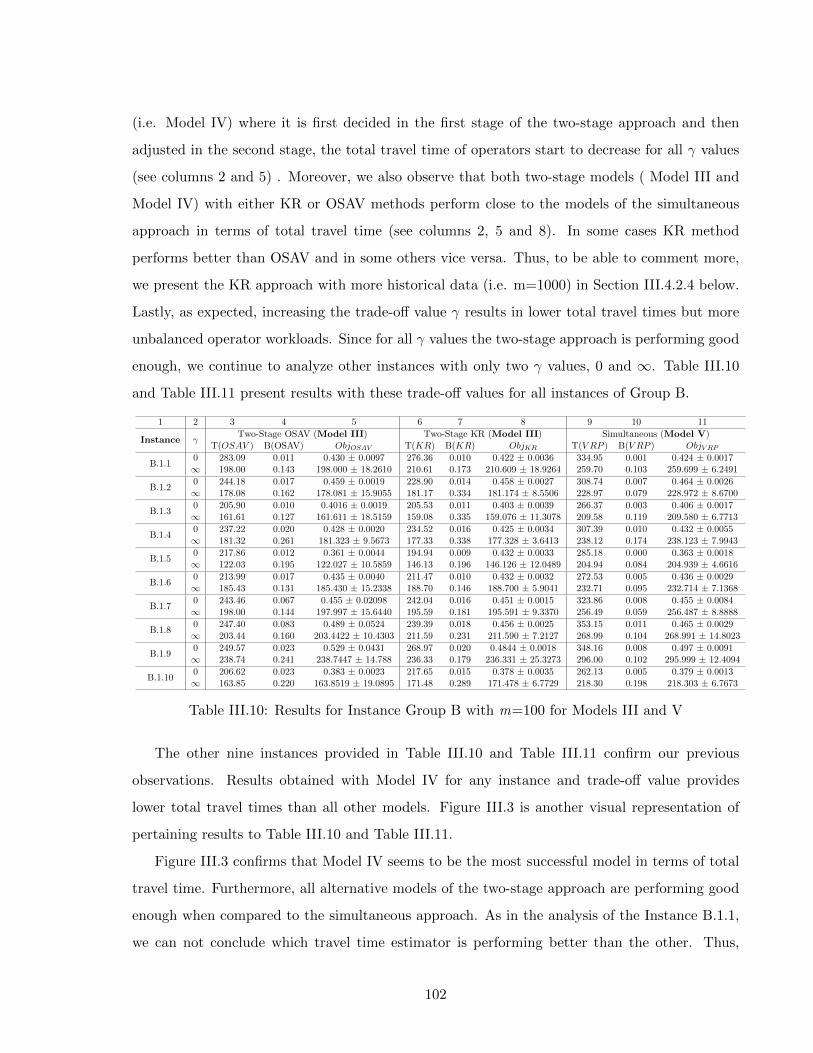
(i.e. Model IV) where it is first decided in the first stage of the two-stage approach and then
adjusted in the second stage, the total travel time of operators start to decrease for all γ values
(see columns 2 and 5) . Moreover, we also observe that both two-stage models ( Model III and
Model IV) with either KR or OSAV methods perform close to the models of the simultaneous
approach in terms of total travel time (see columns 2, 5 and 8). In some cases KR method
performs better than OSAV and in some others vice versa. Thus, to be able to comment more,
we present the KR approach with more historical data (i.e. m=1000) in Section III.4.2.4 below.
Lastly, as expected, increasing the trade-off value γ results in lower total travel times but more
unbalanced operator workloads. Since for all γ values the two-stage approach is performing good
enough, we continue to analyze other instances with only two γ values, 0 and ∞. Table III.10
and Table III.11 present results with these trade-off values for all instances of Group B.
1 2 3 4 5 6 7 8 9 10 11
Instance γTwo-Stage OSAV (Model III) Two-Stage KR (Model III) Simultaneous (Model V)
T(OSAV ) B(OSAV) ObjOSAV T(KR) B(KR) ObjKR T(V RP ) B(V RP ) ObjV RP
B.1.10 283.09 0.011 0.430 ± 0.0097 276.36 0.010 0.422 ± 0.0036 334.95 0.001 0.424 ± 0.0017∞ 198.00 0.143 198.000 ± 18.2610 210.61 0.173 210.609 ± 18.9264 259.70 0.103 259.699 ± 6.2491
B.1.20 244.18 0.017 0.459 ± 0.0019 228.90 0.014 0.458 ± 0.0027 308.74 0.007 0.464 ± 0.0026∞ 178.08 0.162 178.081 ± 15.9055 181.17 0.334 181.174 ± 8.5506 228.97 0.079 228.972 ± 8.6700
B.1.30 205.90 0.010 0.4016 ± 0.0019 205.53 0.011 0.403 ± 0.0039 266.37 0.003 0.406 ± 0.0017∞ 161.61 0.127 161.611 ± 18.5159 159.08 0.335 159.076 ± 11.3078 209.58 0.119 209.580 ± 6.7713
B.1.40 237.22 0.020 0.428 ± 0.0020 234.52 0.016 0.425 ± 0.0034 307.39 0.010 0.432 ± 0.0055∞ 181.32 0.261 181.323 ± 9.5673 177.33 0.338 177.328 ± 3.6413 238.12 0.174 238.123 ± 7.9943
B.1.50 217.86 0.012 0.361 ± 0.0044 194.94 0.009 0.432 ± 0.0033 285.18 0.000 0.363 ± 0.0018∞ 122.03 0.195 122.027 ± 10.5859 146.13 0.196 146.126 ± 12.0489 204.94 0.084 204.939 ± 4.6616
B.1.60 213.99 0.017 0.435 ± 0.0040 211.47 0.010 0.432 ± 0.0032 272.53 0.005 0.436 ± 0.0029∞ 185.43 0.131 185.430 ± 15.2338 188.70 0.146 188.700 ± 5.9041 232.71 0.095 232.714 ± 7.1368
B.1.70 243.46 0.067 0.455 ± 0.02098 242.04 0.016 0.451 ± 0.0015 323.86 0.008 0.455 ± 0.0084∞ 198.00 0.144 197.997 ± 15.6440 195.59 0.181 195.591 ± 9.3370 256.49 0.059 256.487 ± 8.8888
B.1.80 247.40 0.083 0.489 ± 0.0524 239.39 0.018 0.456 ± 0.0025 353.15 0.011 0.465 ± 0.0029∞ 203.44 0.160 203.4422 ± 10.4303 211.59 0.231 211.590 ± 7.2127 268.99 0.104 268.991 ± 14.8023
B.1.90 249.57 0.023 0.529 ± 0.0431 268.97 0.020 0.4844 ± 0.0018 348.16 0.008 0.497 ± 0.0091∞ 238.74 0.241 238.7447 ± 14.788 236.33 0.179 236.331 ± 25.3273 296.00 0.102 295.999 ± 12.4094
B.1.100 206.62 0.023 0.383 ± 0.0023 217.65 0.015 0.378 ± 0.0035 262.13 0.005 0.379 ± 0.0013∞ 163.85 0.220 163.8519 ± 19.0895 171.48 0.289 171.478 ± 6.7729 218.30 0.198 218.303 ± 6.7673
Table III.10: Results for Instance Group B with m=100 for Models III and V
The other nine instances provided in Table III.10 and Table III.11 confirm our previous
observations. Results obtained with Model IV for any instance and trade-off value provides
lower total travel times than all other models. Figure III.3 is another visual representation of
pertaining results to Table III.10 and Table III.11.
Figure III.3 confirms that Model IV seems to be the most successful model in terms of total
travel time. Furthermore, all alternative models of the two-stage approach are performing good
enough when compared to the simultaneous approach. As in the analysis of the Instance B.1.1,
we can not conclude which travel time estimator is performing better than the other. Thus,
102

1 2 3 4 5 6 7 8 9 10 11
Instance γTwo-Stage OSAV (Model IV) Two-Stage KR (Model IV) Simultaneous (Model V)
T(OSAV ) B(OSAV) ObjOSAV T(KR) B(KR) ObjKR T(V RP ) B(V RP ) ObjV RP
B.1.10 234.50 0.018 0.423 ± 0.0086 259.35 0.014 0.422 ± 0.0056 334.95 0.001 0.424 ± 0.0017∞ 186.32 0.142 186.314 ± 13.042 204.45 0.189 204.448 ± 22.3561 259.70 0.103 259.699 ± 6.2491
B.1.20 225.60 0.013 0.456 ± 0.0020 226.09 0.016 0.458 ± 0.0015 308.74 0.007 0.464 ± 0.0026∞ 167.45 0.163 167.452 ± 10.3921 179.74 0.333 179.742 ± 12.3954 228.97 0.079 228.972 ± 8.6700
B.1.30 186.45 0.013 0.402 ± 0.0032 201.74 0.014 0.405 ± 0.0049 266.37 0.003 0.406 ± 0.0017∞ 156.37 0.130 156.374 ± 15.9795 152.00 0.334 151.999 ± 10.7377 209.58 0.119 209.580 ± 6.7713
B.1.40 221.69 0.023 0.426 ± 0.0011 227.25 0.019 0.425 ± 0.0042 307.39 0.010 0.432 ± 0.0055∞ 180.17 0.244 180.174 ± 6.8892 175.86 0.333 175.859 ± 8.6199 238.12 0.174 238.123 ± 7.9943
B.1.50 204.49 0.012 0.361 ± 0.0067 181.10 0.006 0.354 ± 0.0019 285.18 0.000 0.363 ± 0.0018∞ 119.93 0.211 119.928 ± 15.9631 144.25 0.204 144.253 ± 9.8666 204.94 0.084 204.939 ± 4.6616
B.1.60 173.51 0.016 0.429 ± 0.0032 208.54 0.012 0.432 ± 0.0032 272.53 0.005 0.436 ± 0.0029∞ 160.11 0.107 160.113 ± 12.5401 184.70 0.102 184.6977 ± 2.8198 232.71 0.095 232.714 ± 7.1368
B.1.70 227.08 0.098 0.492 ± 0.0439 229.67 0.022 0.452 ± 0.0025 323.86 0.008 0.455 ± 0.0084∞ 189.38 0.145 189.383 ± 7.1874 188.79 0.180 188.794 ± 19.0097 256.49 0.059 256.487 ± 8.88884
B.1.80 237.53 0.082 0.488 ± 0.0587 229.85 0.023 0.457 ± 0.0039 353.15 0.011 0.465 ± 0.0029∞ 186.21 0.105 186.210 ± 20.2977 210.60 0.228 210.600 ± 11.1603 268.99 0.104 268.991 ± 14.8023
B.1.90 231.90 0.023 0.562 ± 0.0955 255.62 0.021 0.483 ± 0.0038 348.16 0.008 0.497 ± 0.0091∞ 226.96 0.135 226.9577 ± 12.7062 209.99 0.119 209.990 ± 24.6529 296.00 0.102 295.999 ± 12.4094
B.1.100 205.51 0.017 0.378 ± 0.0147 215.54 0.011 0.378 ± 0,0027 262.13 0.005 0.379 ± 0.0013∞ 162.00 0.246 161.996 ±4.1591 167.12 0.290 167.119 ± 14.8358 218.30 0.198 218.303 ± 6.7673
Table III.11: Results for Instance Group B with m=100 for Model IV and V
here below we conduct a sensitivity analysis to investigate the effect of increasing the size of the
historical data on KR in comparison to OSAV. We variate values of γ and GA iterations.
III.4.2.4 Sensitivity Analysis of Group B Instance
We conduct a sensitivity analysis based on different γ, m and GA iteration values.
Figure III.4 presents the comparison between two travel time estimates KR and OSAV. This
figure is generated by solving instances with a single γ (i.e. selected as ∞ ) value for Model III
and Model IV. This case is specifically chosen since setting γ to ∞ is the most unfavorable case
for the KR method.
In this figure, in addition to the previous analysis based on 100 historical data, we also
incorporate the case with 1000 historical data for the KR method. This case is held for two main
reasons. The first one is to show how KR method performs when the size of the historical data
increases even for the most unfavorable case and the second one is to be able to comment on the
comparison between KR and OSAV. Remind that in the previous analysis, we were not able to
provide a general conclusion for these methods.
103
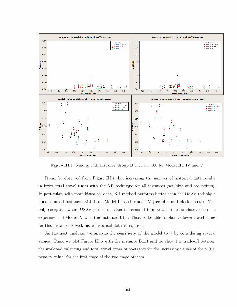
Figure III.3: Results with Instance Group B with m=100 for Model III, IV and V
It can be observed from Figure III.4 that increasing the number of historical data results
in lower total travel times with the KR technique for all instances (see blue and red points).
In particular, with more historical data, KR method performs better than the OSAV technique
almost for all instances with both Model III and Model IV (see blue and black points). The
only exception where OSAV performs better in terms of total travel times is observed on the
experiment of Model IV with the Instance B.1.8. Thus, to be able to observe lower travel times
for this instance as well, more historical data is required.
As the next analysis, we analyze the sensitivity of the model to γ by considering several
values. Thus, we plot Figure III.5 with the instance B.1.1 and we show the trade-off between
the workload balancing and total travel times of operators for the increasing values of the γ (i.e.
penalty value) for the first stage of the two-stage process.
104
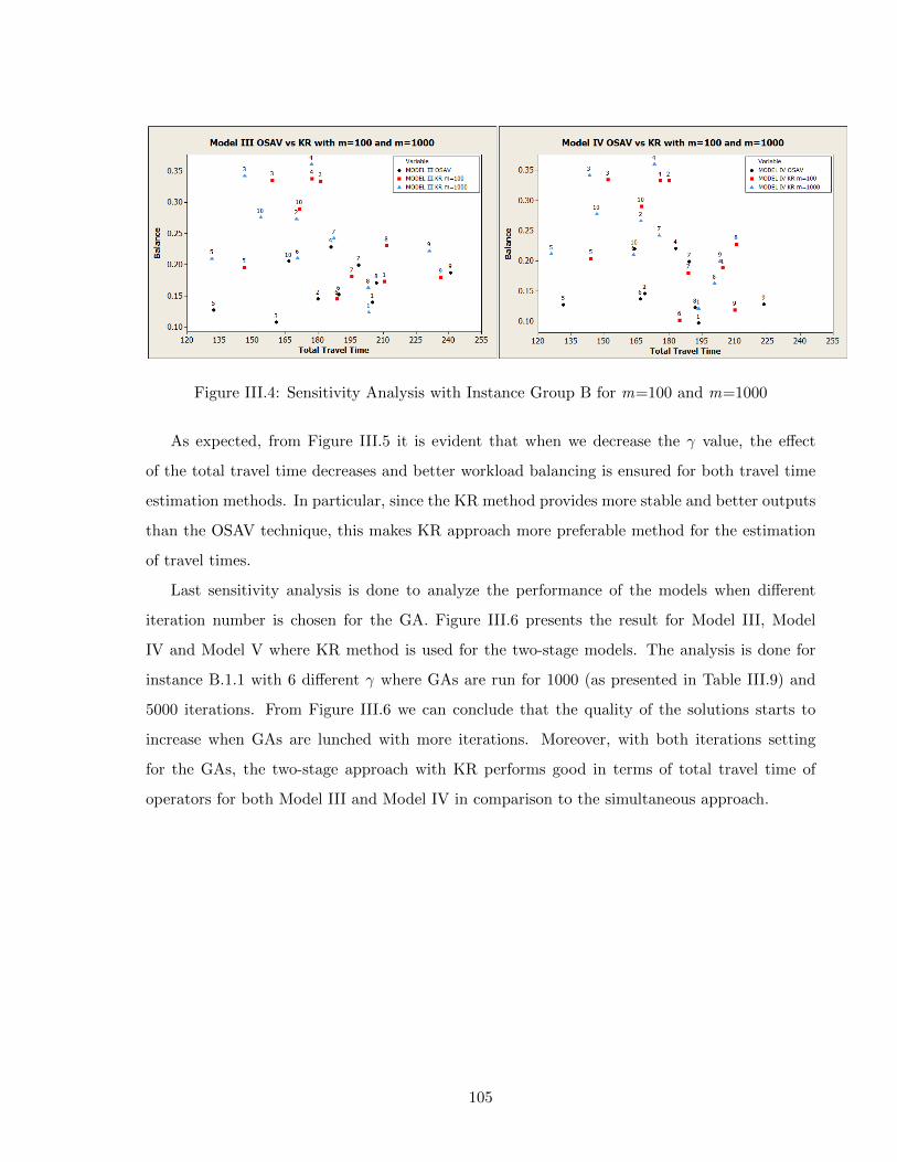
Figure III.4: Sensitivity Analysis with Instance Group B for m=100 and m=1000
As expected, from Figure III.5 it is evident that when we decrease the γ value, the effect
of the total travel time decreases and better workload balancing is ensured for both travel time
estimation methods. In particular, since the KR method provides more stable and better outputs
than the OSAV technique, this makes KR approach more preferable method for the estimation
of travel times.
Last sensitivity analysis is done to analyze the performance of the models when different
iteration number is chosen for the GA. Figure III.6 presents the result for Model III, Model
IV and Model V where KR method is used for the two-stage models. The analysis is done for
instance B.1.1 with 6 different γ where GAs are run for 1000 (as presented in Table III.9) and
5000 iterations. From Figure III.6 we can conclude that the quality of the solutions starts to
increase when GAs are lunched with more iterations. Moreover, with both iterations setting
for the GAs, the two-stage approach with KR performs good in terms of total travel time of
operators for both Model III and Model IV in comparison to the simultaneous approach.
105
III.5 CONCLUSION
In this part, we analyze the impact of the travel time estimation methods especially the KR
technique in a two-stage planning approach. We conduct several experiments with different
modeling assumptions such as single or multiple planning periods, existing or relaxed operator
capacities restrictions. All assumptions are tested with two-stage models, Model I, Model III
and Model IV and compared to the simultaneous approach models, Model V.
As the result of all these experiments and analysis, we see that the two-stage approach with
KR method provides similar results to those of the simultaneous approach. Particularly, adjusting
the care plan decision, which is initially held in the assignment stage of the two-stage approach,
in the routing stage provides lower total travel times (i.e. results with Model IV). Another
important observation is based on the size of the historical data. As the size of the historical
data increases (i.e. m = 1000), the total travel time values start to decrease as well. Hence,
we can conclude that the KR technique used in Model IV with a realistic number of historical
data seems to be a promising tool for approximately solving the HHC VRP (i.e m = 1000 can
be considered as a realistic case since an operator usually works 250 days per year).
The experiments in this part have some limitations. For example, operator qualifications has
not been considered while analyzing the travel time estimation methods. Thus, one important
extension will be to include operator skills to analyze more realistic situations. Another limitation
is only focusing on the geographical locations of patients which actually might not be the only
criteria for defining operators’ visits. In some cases, operators might also need to consider other
significant HHC specific features while planning their visits, such as patients’ care profiles (i.e.,
corresponding pathology), special service requests (i.e., requests for clinical tests) and temporal
constraints (i.e., requests for visits at specific times). Using these features is also important
for capturing real operator behaviors and estimating more accurate travel times. Lastly, an
exact solution approach based on the Column Generation method can be implemented to better
analyze the performance of the travel time estimators and the two-stage approach.
106

Figure III.5: The Trade-Off Anaylsis for the Assignment Phase Of the Two-Stage Model withthe KR and OSAV methods with m=100
Figure III.6: Sensitivity Analysis on the Iteration Number of the GA with Instance B.1.1 andm=100
107

Part IV
ASSESSING THE IMPACT OF THE SKILL MANAGEMENT
108

IV.1 INTRODUCTION
In this part, we present the results of the two-stage models considering different patient require-
ments and different operators skills. The issue of different requirements/skills is relevant from
a practical perspective since patients would often require various services that can be grouped
as regular or specific/intensive requirements. These services are usually provided by operators
having different abilities. For instance, patients with regular requirements would be served by
operators having basic skills whereas patients having intensive requirements should be cared by
more qualified operators. Hence, the health care provider has to manage skill compatibility is-
sues to ensure that the required skill is deployed for a given type of patient requirement. Note
that, generally operators that are able to serve patients with intensive requirements are capable
to serve regular patients as well. Thus, the HHC providers can either manage operator skills
independently (i.e. without allowing an overskilled operator performing care activities that re-
quire a lower level of skill) or they can use more qualified operators for basic services as well
(i.e. hierarchial skill management). Hence, the goal of this section is to analyze the impact of
the alternative skill management ways (i.e. independent or hierarchical skill management) on
the two-stage approach and compare the impact with the ones of the simultaneous planning
approaches.
The alternative modeling variants of the two-stage approach presented in Figure II.1 (cf.
Chapter II) for the multiple planning periods are tested on several instances. Daily operator
capacity restrictions are considered in all experiments.
In Section IV.2, details of the experiments are presented. Then, in Section IV.3, parameter
settings for the instances and solution methods are identified. Finally, numerical results and the
corresponding analysis are presented in Section IV.4.
IV.2 DESIGN OF EXPERIMENTS
Experiments are done based on a single instance group (Group C) generated from real data.
We consider three sets of instances depending on the size of instances, (i.e. one medium-sized,
Group C.1, and two large-sized sets, Group C.2 and C.3). These instances are used for both the
two-stage and simultaneous approach models with different operator and patient skills, multiple
planning periods and operator capacity restriction assumptions.
109

Several two-stage modeling scenarios are considered (i.e Model II, Model III and Model IV)
and compared to the simultaneous models (i.e. Model V). With Group C.1 instances, Model II,
Model III and Model IV are used for the two-stage approach with independent and hierarchical
skills. Then, as the result of the analysis made on these models, the best model in terms of
solution quality is identified (i.e. Model IV) and used for further analysis with Group C.2 and
C.3 instances.
The two-stage models are solved by only considering the AV approach as the travel time
estimation method for the first stage of the two-stage approach. In particular, two different
objective functions are used to solve each model where the first one is the balancing objective
(i.e. minimizing the maximum operator utilization factor, MinMax) and the second one is the
cost minimization objective (i.e. minimizing total travel time of all operators, MinCost). The
formulation of these objectives in the simultaneous approach is straightforward. On the other
hand, the formulation of these two objectives for the two-stage approach needs more attention.
Thus, when we refer to the case of balancing objective (MinMax), we try to minimize the max-
imum operator utilization factor in the both objective functions. However, when we consider
the travel time minimization objective (MinCost), we use balancing objective in the first stage
and travel time minimization in the second stage. Since the assignment problem (i.e. first stage
problem) is already solved to balance the workloads of operators, we try to analyze if it is worth
to consider by possibly increasing the tour lengths of some operators and balance the workloads
in the second stage problem as well (with MinMax objective).
In the following section, we present the selected parameter settings of the considered instances
and solution methods in more details.
IV.3 EXPERIMENTAL SETTINGS
In this section, we present the details of the instance and solution method parameter settings
respectively.
IV.3.1 Parameters Regarding the Instances
Group C:
• 2 skill levels are assumed for patients.
110
1. Skill 1 (i.e. patients having regular requirements) and Skill 2 patients (i.e. patients
having with intensive requirements)
• 2 skill levels are assumed for operators.
1. Skill 1 (i.e. ability to care patients with regular requirements) and Skill 2 operators
(i.e. ability to care patients with regular and intensive requirements)
• A total of 20 instances are grouped in three sets and used in Group C experiments, see
Table IV.1 for all the details.
1. The first set of instances consists of 10 medium-size instances (i.e. Group C.1). Those
are identified between C.1.1 and C.1.10 that consider 60 patients and 4 operators.
(a) Group C.1: 44 to 56 skill 1, 4 to 16 skill 2 patients and 2 skill 1, 2 skill 2 operators.
2. The second and third set of instances consists in total of 10 large-size instances (i.e.
Group C.2 and Group C.3). The second set is identified between C.2.1 and C.2.5 for
Group C.2 that consider 100 patients and 7 operators. The third set of the instances
are identified between C.3.1 and C.3.5 for Group C.3 that consider 200 patients and
10 operators.
(a) Group C.2: 80 to 88 skill 1, 12 to 20 skill 2 patients and 4 skill 1, 3 skill 2
operators.
(b) Group C.3: 159 to 174 skill 1, 26 to 41 skill 2 patients and 6 skill 1, 4 skill 2
operators.
• Daily operator capacities for each instance are as follows:
1. Group C.1: 400 and 350 minutes respectively for skill 1 operators and 300 minutes
for each skill 2 operator.
2. Group C.2: 400, 350, 300 and 300 minutes respectively for skill 1 operators and 300
minutes for each skill 2 operator.
3. Group C.3: 500, 500, 400, 400, 350, 350 minutes respectively for skill 1 operators and
300 minutes for each skill 2 operator.
• All the instances in each set is directly generated from read data, with 60, 100 and 200
patients and distributed across 7 cities as it is in Part III.
111
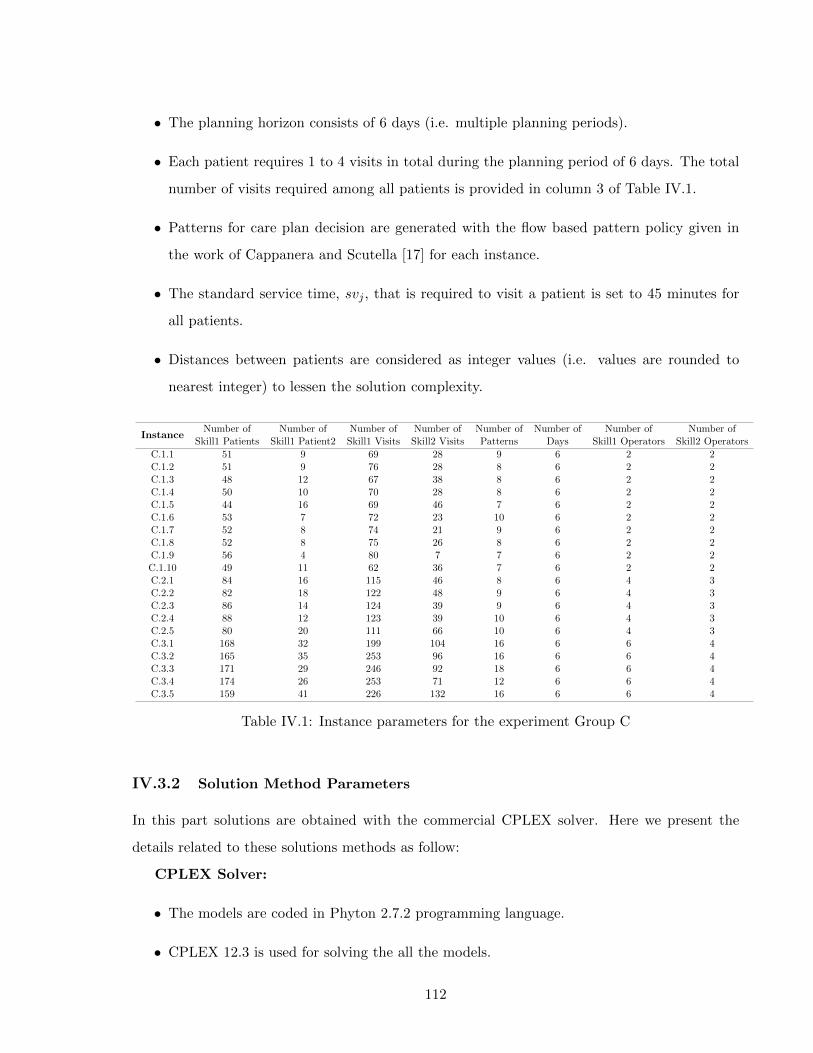
• The planning horizon consists of 6 days (i.e. multiple planning periods).
• Each patient requires 1 to 4 visits in total during the planning period of 6 days. The total
number of visits required among all patients is provided in column 3 of Table IV.1.
• Patterns for care plan decision are generated with the flow based pattern policy given in
the work of Cappanera and Scutella [17] for each instance.
• The standard service time, svj , that is required to visit a patient is set to 45 minutes for
all patients.
• Distances between patients are considered as integer values (i.e. values are rounded to
nearest integer) to lessen the solution complexity.
InstanceNumber of Number of Number of Number of Number of Number of Number of Number of
Skill1 Patients Skill1 Patient2 Skill1 Visits Skill2 Visits Patterns Days Skill1 Operators Skill2 Operators
C.1.1 51 9 69 28 9 6 2 2C.1.2 51 9 76 28 8 6 2 2C.1.3 48 12 67 38 8 6 2 2C.1.4 50 10 70 28 8 6 2 2C.1.5 44 16 69 46 7 6 2 2C.1.6 53 7 72 23 10 6 2 2C.1.7 52 8 74 21 9 6 2 2C.1.8 52 8 75 26 8 6 2 2C.1.9 56 4 80 7 7 6 2 2C.1.10 49 11 62 36 7 6 2 2C.2.1 84 16 115 46 8 6 4 3C.2.2 82 18 122 48 9 6 4 3C.2.3 86 14 124 39 9 6 4 3C.2.4 88 12 123 39 10 6 4 3C.2.5 80 20 111 66 10 6 4 3C.3.1 168 32 199 104 16 6 6 4C.3.2 165 35 253 96 16 6 6 4C.3.3 171 29 246 92 18 6 6 4C.3.4 174 26 253 71 12 6 6 4C.3.5 159 41 226 132 16 6 6 4
Table IV.1: Instance parameters for the experiment Group C
IV.3.2 Solution Method Parameters
In this part solutions are obtained with the commercial CPLEX solver. Here we present the
details related to these solutions methods as follow:
CPLEX Solver:
• The models are coded in Phyton 2.7.2 programming language.
• CPLEX 12.3 is used for solving the all the models.
112

• CPU time limit is set as 12 hours.
• Memory limit is set equal to 1 Gb.
• In the tables that are presented in numerical result section, a ? is used to denote an instance
for which the memory limit is exceeded and a is used to show that the presented results
are reported with the upper CPU time limit.
Note that, all these numerical experiments are performed on a computer with Intel Core i.7
2.2 GHz CPU, and 8 GB of RAM.
IV.4 NUMERICAL RESULTS
The proposed two-stage models with hierarchical and independent skills are tested and com-
pared to the simultaneous approach. We start by presenting the performance indicators used
to analyze the results. Then, numerical results with Model II, Model III, Model IV and Model
V are provided. With the provided results, we try to analyze the the impact of different skill
management cases on the two-stage and simultaneous approaches. In particular, by using dif-
ferent modeling scenarios for the two-stage approach, we try to investigate the best model to
consider the assignment, care plan and routing decisions via two-stage approach. Hence, we start
solving all the indicated models with the medium-sized instances and then extend our analysis
with large-sized instances by only considering the best two-stage model among the alternatives.
For all the set of the instances models of the simultaneous approach are solved and compared
with the ones of the two-stage approach as well.
IV.4.1 Performance Indicators
Four indicators are used to assess the performance of each model analyzed. Total travel time
of all operators obtained in the two-stage and simultaneous approaches is shown by T , and the
workload balance value between the maximally and minimally utilized operators is shown by B.
The models are solved with either balancing (i.e. MinMax) or cost minimization (i.e. MinCost)
objectives thus, the corresponding objective function value is denoted as Obj and is either set
equal to h or T value where h corresponds to the maximum operator utilization level. Lastly,
NOvSk is used for the hierarchial skill case. It is used to denote the total number of times that
113

operators with skill level 2 are used for lower skilled patients (i.e. with patients belonging to skill
level 1) for the models with hierarchical skill consideration.
The T values for the two-stage models are obtained by solving several independent TSP
models either with balancing or travel time minimization objectives with the outputs obtained
from the assignment stage and summing the results of each TSP model across the all opera-
tors. On the other hand, T values for the simultaneous models are directly calculated from the
corresponding model as the sum of each operator’s route time.
IV.4.2 Results
We first present the results for the medium-sized instances (i.e. Group C.1) to compare Model
II, Model III and Model IV of the two-stage approach with the models of the simultaneous
approach. Then we also provide results with the best performing two-stage model (according
to the analysis based on Group C.1 instances) and corresponding simultaneous model for the
large-sized instances (i.e. Group C.2 and Group C.3). All the instances are solved with the
independent and hierarchical skill cases by considering both the balancing and cost minimization
objectives.
IV.4.2.1 Results with the Instance Group C
We consider three subset of instances for Group C to analyze the models with 2 skill levels,
multiple planning periods and operator capacity restrictions.
Results for Group C.1 Instances:
Table IV.2 and Table IV.3 provide results for Model III, Model IV and Model V with the
hierarchical operator skills. Regarding the solutions of the independent skill case where an
operator can perform only the visits requiring exactly his/her skill, all of the instances turn
out to be infeasible. One possible cause of this infeasibility might be the insufficient number of
patterns. However, when the skills are managed hierarchically, we are able to obtain feasible
solutions for the two-stage and simultaneous models with most of the instances even with the
same pattern sets. The only exception is observed for Model II of the two-stage approach. Results
of this model also turns out to be in feasible with all of the instances except the Instance C.1.9.
The reason for these infeasibilities are also possibly the number of used pattern.
Although we observe infeasibilities in some cases due to limited number of pattern, we con-
114
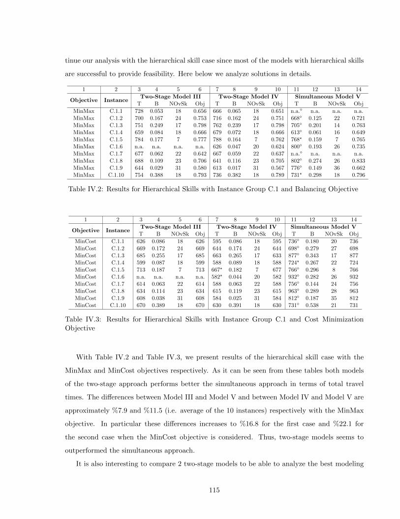
tinue our analysis with the hierarchical skill case since most of the models with hierarchical skills
are successful to provide feasibility. Here below we analyze solutions in details.
1 2 3 4 5 6 7 8 9 10 11 12 13 14
Objective InstanceTwo-Stage Model III Two-Stage Model IV Simultaneous Model V
T B NOvSk Obj T B NOvSk Obj T B NOvSk Obj
MinMax C.1.1 728 0.053 18 0.656 666 0.065 18 0.651 n.a. n.a. n.a. n.a.MinMax C.1.2 700 0.167 24 0.753 716 0.162 24 0.751 668 0.125 22 0.721MinMax C.1.3 751 0.249 17 0.798 762 0.239 17 0.798 705 0.201 14 0.763MinMax C.1.4 659 0.084 18 0.666 679 0.072 18 0.666 613 0.061 16 0.649MinMax C.1.5 784 0.177 7 0.777 788 0.164 7 0.762 768? 0.159 7 0.765MinMax C.1.6 n.a. n.a. n.a. n.a. 626 0.047 20 0.624 800 0.193 26 0.735MinMax C.1.7 677 0.062 22 0.642 667 0.059 22 0.637 n.a. n.a. n.a. n.a.MinMax C.1.8 688 0.109 23 0.706 641 0.116 23 0.705 802 0.274 26 0.833MinMax C.1.9 644 0.029 31 0.580 613 0.017 31 0.567 776 0.149 36 0.662MinMax C.1.10 754 0.388 18 0.793 736 0.382 18 0.789 731? 0.298 18 0.796
Table IV.2: Results for Hierarchical Skills with Instance Group C.1 and Balancing Objective
1 2 3 4 5 6 7 8 9 10 11 12 13 14
Objective InstanceTwo-Stage Model III Two-Stage Model IV Simultaneous Model VT B NOvSk Obj T B NOvSk Obj T B NOvSk Obj
MinCost C.1.1 626 0.086 18 626 595 0.086 18 595 736 0.180 20 736MinCost C.1.2 669 0.172 24 669 644 0.174 24 644 698 0.279 27 698MinCost C.1.3 685 0.255 17 685 663 0.265 17 633 877 0.343 17 877MinCost C.1.4 599 0.087 18 599 588 0.089 18 588 724? 0.267 22 724MinCost C.1.5 713 0.187 7 713 667? 0.182 7 677 766 0.296 8 766MinCost C.1.6 n.a. n.a. n.a. n.a. 582? 0.044 20 582 932 0.282 26 932MinCost C.1.7 614 0.063 22 614 588 0.063 22 588 756 0.144 24 756MinCost C.1.8 634 0.114 23 634 615 0.119 23 615 963 0.289 28 963MinCost C.1.9 608 0.038 31 608 584 0.025 31 584 812 0.187 35 812MinCost C.1.10 670 0.389 18 670 630 0.391 18 630 731 0.538 21 731
Table IV.3: Results for Hierarchical Skills with Instance Group C.1 and Cost MinimizationObjective
With Table IV.2 and Table IV.3, we present results of the hierarchical skill case with the
MinMax and MinCost objectives respectively. As it can be seen from these tables both models
of the two-stage approach performs better the simultaneous approach in terms of total travel
times. The differences between Model III and Model V and between Model IV and Model V are
approximately %7.9 and %11.5 (i.e. average of the 10 instances) respectively with the MinMax
objective. In particular these differences increases to %16.8 for the first case and %22.1 for
the second case when the MinCost objective is considered. Thus, two-stage models seems to
outperformed the simultaneous approach.
It is also interesting to compare 2 two-stage models to be able to analyze the best modeling
115
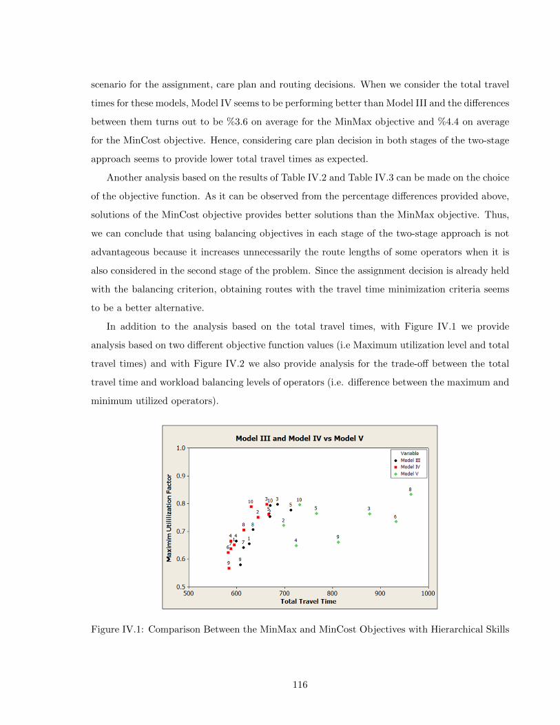
scenario for the assignment, care plan and routing decisions. When we consider the total travel
times for these models, Model IV seems to be performing better than Model III and the differences
between them turns out to be %3.6 on average for the MinMax objective and %4.4 on average
for the MinCost objective. Hence, considering care plan decision in both stages of the two-stage
approach seems to provide lower total travel times as expected.
Another analysis based on the results of Table IV.2 and Table IV.3 can be made on the choice
of the objective function. As it can be observed from the percentage differences provided above,
solutions of the MinCost objective provides better solutions than the MinMax objective. Thus,
we can conclude that using balancing objectives in each stage of the two-stage approach is not
advantageous because it increases unnecessarily the route lengths of some operators when it is
also considered in the second stage of the problem. Since the assignment decision is already held
with the balancing criterion, obtaining routes with the travel time minimization criteria seems
to be a better alternative.
In addition to the analysis based on the total travel times, with Figure IV.1 we provide
analysis based on two different objective function values (i.e Maximum utilization level and total
travel times) and with Figure IV.2 we also provide analysis for the trade-off between the total
travel time and workload balancing levels of operators (i.e. difference between the maximum and
minimum utilized operators).
Figure IV.1: Comparison Between the MinMax and MinCost Objectives with Hierarchical Skills
116

Figure IV.2: Trade-off Analysis for MinMax and MinCost Objectives with Hierarchical Skillswith Medium-Sized Instances
Similar to the previous analysis, from Figure IV.1 it can be observed that two-stage models
and especially Model IV provides better solutions (i.e. more balanced workloads with lower total
travel time) by considering both objective function values (i.e. Obj values). In particular, from
Figure IV.2 we can see that MinCost objective provides more stable and better solutions than
the MinMax objective.
Hence, from all these analysis we can conclude that if we manage different skills in a hierarchi-
cal way, we are able to obtain feasible and interesting results. In particular, we also observe that
making the assignment, care plan and routing decisions via two stage approach provides better
solutions (i.e. in terms of balancing and total travel time) than the ones of the simultaneous
approach especially with the MinCost objective. Particularly, the best alternative is observed
when the first stage care plan decision is modified in the second stage of the problem (i.e. Model
IV).
In the following part, we extend the analysis with large-size instances by considering the best
performing two-stage model (i.e. Model IV) and the simultaneous model.
Results for Group C.2 and C.3 Instances:
Here we present results with larger instances. Similar to the previous analysis of the medium-
size instances, we can not obtain any feasible solution for the independent skill case. In addition
117
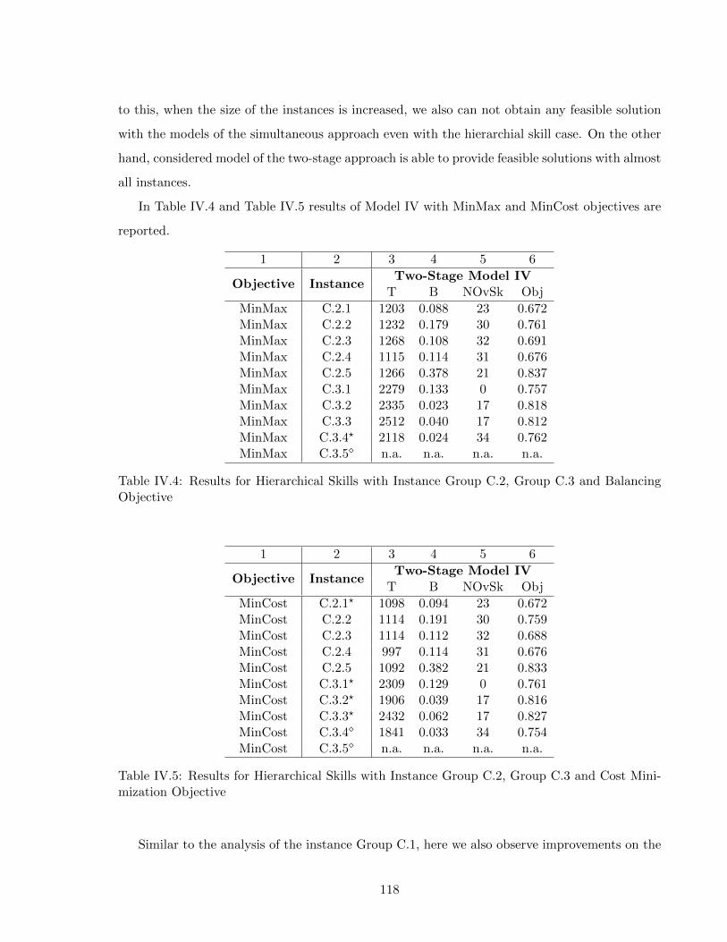
to this, when the size of the instances is increased, we also can not obtain any feasible solution
with the models of the simultaneous approach even with the hierarchial skill case. On the other
hand, considered model of the two-stage approach is able to provide feasible solutions with almost
all instances.
In Table IV.4 and Table IV.5 results of Model IV with MinMax and MinCost objectives are
reported.
1 2 3 4 5 6
Objective InstanceTwo-Stage Model IV
T B NOvSk Obj
MinMax C.2.1 1203 0.088 23 0.672MinMax C.2.2 1232 0.179 30 0.761MinMax C.2.3 1268 0.108 32 0.691MinMax C.2.4 1115 0.114 31 0.676MinMax C.2.5 1266 0.378 21 0.837MinMax C.3.1 2279 0.133 0 0.757MinMax C.3.2 2335 0.023 17 0.818MinMax C.3.3 2512 0.040 17 0.812MinMax C.3.4? 2118 0.024 34 0.762MinMax C.3.5 n.a. n.a. n.a. n.a.
Table IV.4: Results for Hierarchical Skills with Instance Group C.2, Group C.3 and BalancingObjective
1 2 3 4 5 6
Objective InstanceTwo-Stage Model IV
T B NOvSk Obj
MinCost C.2.1? 1098 0.094 23 0.672MinCost C.2.2 1114 0.191 30 0.759MinCost C.2.3 1114 0.112 32 0.688MinCost C.2.4 997 0.114 31 0.676MinCost C.2.5 1092 0.382 21 0.833MinCost C.3.1? 2309 0.129 0 0.761MinCost C.3.2? 1906 0.039 17 0.816MinCost C.3.3? 2432 0.062 17 0.827MinCost C.3.4 1841 0.033 34 0.754MinCost C.3.5 n.a. n.a. n.a. n.a.
Table IV.5: Results for Hierarchical Skills with Instance Group C.2, Group C.3 and Cost Mini-mization Objective
Similar to the analysis of the instance Group C.1, here we also observe improvements on the
118
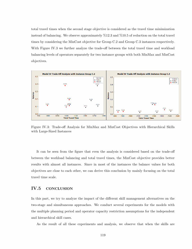
total travel times when the second stage objective is considered as the travel time minimization
instead of balancing. We observe approximately %12.3 and %10.5 of reduction on the total travel
times by considering the MinCost objective for Group C.2 and Group C.3 instances respectively.
With Figure IV.3 we further analyze the trade-off between the total travel time and workload
balancing levels of operators separately for two instance groups with both MinMax and MinCost
objectives.
Figure IV.3: Trade-off Analysis for MinMax and MinCost Objectives with Hierarchical Skillswith Large-Sized Instances
It can be seen from the figure that even the analysis is considered based on the trade-off
between the workload balancing and total travel times, the MinCost objective provides better
results with almost all instances. Since in most of the instances the balance values for both
objectives are close to each other, we can derive this conclusion by mainly focusing on the total
travel time scale.
IV.5 CONCLUSION
In this part, we try to analyze the impact of the different skill management alternatives on the
two-stage and simultaneous approaches. We conduct several experiments for the models with
the multiple planning period and operator capacity restriction assumptions for the independent
and hierarchical skill cases.
As the result of all these experiments and analysis, we observe that when the skills are
119
managed independently, we could not obtain any feasible solutions. On the other hand, hierar-
chically considering the skills helps us to obtain feasible solutions with both the two-stage and
simultaneous approaches.
We also see that the solutions of the two-stage models outperformed the solutions of the
simultaneous models. Especially, when the size of the instances are increased the simultaneous
approach does not make possible providing feasible solutions whereas the two-stage approach
does. Moreover, for the two-stage models considering the assignment problem with the balancing
objective and routing problem with the cost minimization objective provides the best solutions.
Additionally, we also compare three modeling scenarios for deciding the assignment, care plan
and routing decisions for the two-stage models. This comparison shows us that considering the
care plan decision in both stages seems to be the best alternative modeling case.
One limitation regarding to the experiments of this part can be considered as the number of
patterns used to solve the models. Due to limited number of patterns, we are not able to observe
feasible solutions for the independent skill case. Thus, it will be interesting to repeat all these
experiments with the increased number of patterns and compare the corresponding solutions with
ones of the hierarchical skill case. Another extension can be done by considering data-driven
travel time estimation method (i.e. KR approach) instead of using the AV approach. In the
previous part (see Part III), we show that the performance of the KR approach outperforms the
AV approach. Hence, all the reported solutions of this part can be improved by considering the
KR technique.
120
Chapter 6
CONCLUSION AND PERSPECTIVES
6.1 CONCLUSION
In this study, we develop new methods and models to support the human resource planning
process of the HHC services. We particularly focus on the assignment and routing problems of
the human resource planning process. To this end, we first consider an alternative and more
convenient method than the widely used simultaneous approach. Hence, we focus on the two-
stage approach that is an approximate approach for sequentially solving the assignment and
routing problems rather than solving them at the same time. We propose several two-stage
models with various realistic assumptions such as skill compatibility between operators and
patients, multiple planning periods and operator capacity restrictions. Then, we analyze the
performance of these models in comparison to the simultaneous approach models. In particular,
since the assignment decision of the two-stage approach is typically made without knowing the
visiting sequence, we also need to consider good travel time estimates for being used in the
assignment problem. Thus, we propose a Kernel Regression method to estimate travel times
using the historical routing information of the operators. Then, we analyze the performance of
the proposed estimator and show the improvements achieved in comparison with the AV and
OSAV methods via two-stage approach.
As a result of a comprehensive computational study, we observe that the solutions of the
two-stage approach are comparable with the simultaneous approach and this process seems to be
a promising tool for approximately solving the HHC VRP. It is observed that the use of the KR
technique is promising as well in practical HHC organizations where the number of patients and
operators can be significant and the assignment and routing problems have different time scales,
e.g. operators’ assignment lists are gathered weekly, and routes are obtained daily. In particular,
121
among different skill management alternatives, the hierarchical skill case turns out to be a better
alterative than the independent skill case with feasible solution for almost all instances. Lastly,
among several modeling alternatives for the two-stage approach (See Figure II.1 in Chapter 2
Part II), it is seen that the Model IV, where the care plan decision is held in both stages, turns
out to be the best alternative with lower total travel times and equitably distributed workload
balancing levels.
As presented in the previous chapters, there are some limitation of this research and so
several research paths to follow. For example, while estimating the travel times of operators with
the KR method, we only consider the geographical locations of patients. However, to capture
real operator behavior, we also need to consider other features such as patients’ care profiles,
special service requests and temporal constraints. Hence, as a future work more accurate travel
time estimates can be obtained by using these features. In particular, KR estimates can be
further improved by using analytical approximations. In the current setting, KR uses a spatial
correlation function (generally radial basis functions) to build a predictor in the unobserved
domain space. However, the knowledge from analytical methods about some structural properties
of the function can help to build the estimator, particularly when the point we want to evaluate
is far from unobserved points and spatial correlation is not likely to hold. Another limitation
of this research is based on the solution approach. Since our main goal in this research is
towards modeling approaches, we do not intent to propose efficient solution algorithms and we
use basic solution methods based on GA and CPLEX solver. However, to better analyze the
performance of two-stage approach (i.e. with any travel time estimation method) with respect
to the simultaneous approach, an efficient exact solution method (i.e. Column Generation) could
be useful and provide more transparent analysis. Such approach could also enable to avoid the
randomness occur due to use of GA or it could decrease the time of finding feasible solutions for
the complex cases (i.e. solving the simultaneous approach with the instance Group C.3) when
the CPLEX solver is used. Lastly, in this research we assume equal costs for different skill levels
while using the hierarchial skill case. Although using this case is more efficient, it could increase
the total resource cost incurred when we assume different costs for different skill levels. Thus, a
further analysis with different cost policies should be investigated as a future work.
122

Bibliography
[1] Akjiratikarl C., Yenradee P., Drake P.R.: PSO-based algorithm for home care worker
scheduling in the UK, Computers and Industrial engineering, 53, 559–583, (2007).
[2] Asquer G., Borsani V., Matta A.: Analysis of the organizational structure of the home
care providers (in Italian), Politiche Sanitarie, 8, 95–117, (2007).
[3] Begur S.V., Miller D.M., Weaver J.R.: An integrated spatial Decision Support System for
scheduling and routing home health care nurses, Interfaces, 27, 35–48, (1997).
[4] Bektas T.: The multiple traveling salesman problem: an overview of formulations and
solution procedures, Omega, 34, 209–219, (2006).
[5] Ben Bachouch R., Fakhfakh M., Guinet A., Hajri-Gabouj S.: Planification de la tournee
des infirmiers dans une structure de soins a domicile, Conference Francophone en Gestion
et Ingenierie des Systemes Hospitaliers (GISEH), Switzerland, (2008).
[6] Ben Bachouch R., Fakhfakh M., Guinet A., Hajri-Gabouj S.: A model for scheduling drug
deliveries in a French homecare, International Conference on Industrial Engineering and
Systems Management (IESM), Montreal, Canada, (2009).
[7] Ben Bachouch R.: Pilotage operationnel des structures d’hospitalisation a domicile, These
de doctorat de l’Institut national des sciences appliques de Lyon, (2010).
[8] Benzarti E., Sahin E., Dallery Y.: Operations management applied to home care services:
Analysis of the districting problem. Decision Support Systems 55, 587–598, (2013).
[9] Benzarti E.: Home health care operations management: applying the districting approach
to home health care, Ph.D Thesis, Ecole Centrale Paris, (2012).
123
[10] Bertels S., Fahle T.: A hybrid setup for a hybrid scenario: combining heuristics for the
home health care problem, Computers and Operations Research, 33, 2866–2890, (2006).
[11] Bredstorm D., Ronnqvist M.: A branch and price algorithm for the combined vehicle rout-
ing and scheduling problem with synchronization constraints. Technical report, Depart-
ment of Finance and Management Science, Norwegian School of Economics and Business
Administration, (2007).
[12] Bredstorm D. and Ronnqvist M.: Combined vehicle routing and scheduling with temporal
precedence and synchronization constraints, European Journal of Operational Research,
191(1), 19–31, (2008).
[13] Brucker P., Qu R., Burke E.: Personnel scheduling: Models and complexity, European
Journal of Operational Research, 210(3), 467–473, (2011).
[14] Bowman A. W. and Azzalini A.: Applied Smoothing Techniques for Data Analysis: The
Kernel Approach with S-Plus Illustrations. Oxford: Oxford University Press., (1997).
[15] Borsani V., Matta A., Beschi G., Sommaruga, F.: A home care scheduling model for human
resources, in Proceedings of Int. Conf. on Service Systems and Service Management, France,
449–454, (2006).
[16] Busby C.R., Carter M.W.: A Decision Tool for Negotiating Home Care Funding Levels in
Ontario, HHC Services Quarterly, 25, p.91-106, (2006).
[17] Cappanera, P., Scutella, M.G.: Joint assignment, scheduling and routing models to home
care optimization: a pattern based approach. Technical Report, TR-13-05, Dipartimento
di Informatica, Universita di Pisa, (2013).
[18] Carello, G., Lanzarone, E.: A cardinality-constrained robust model for the assignment
problem in Home Care services, European Journal of Operational Research, 2, 748–762,
(2014).
[19] Chahed S., Matta A., Sahin E., Dallery Y.: perations management related activities in
home health care structures, Proceedings of INCOM Conference (Information Control
Problems in Manufacturing), Saint–Etienne, France, 3, 641–646, (2006).
124
[20] Chahed S., Marcon E., Sahin E., Feillet D., Dallery Y.: Exploring new operational research
opportunities within the Home Care context: the chemotherapy at home, Health Care
Management Science, 12, 179–191, (2009).
[21] Cheng E., Rich J.L.: A home care routing and scheduling problem. Technical Report TR98-
04, Department of Computational And Applied Mathematics, Rice University, (1998).
[22] Cordeau J.F., Laporte G., Pasin F., Ropke S.: Scheduling technicians and tasks in a
telecommunications company, Journal of Scheduling, 13(4), 393–409, (2010).
[23] De Angelis V.: Planning Home Assistance for AIDS Patients in the City of Rome, Italy,
Interfaces, 28,75–83, (1998).
[24] De Causmaecker P., Demeester P., Vanden Berghe G., Verbeke B.: Analysis of real-world
personnel scheduling problems, in: Proceedings of the 5th International Conference on the
Practice and Theory of Automated Timetabling, Pittsburgh, PA, USA, 183–198, (2005).
[25] Elbenani, B., Ferland, J.A., Gascon, V.: Mathematical Programming Approach for Routing
Home Care Nurses, Proceedings of the 2008 IEEE, (2008)
[26] Ernst, A.T., Jiang, H., Krishnamoorthy, M., Owens, B., Sier, D.: An annotated bibliog-
raphy of personnel scheduling and rostering, Annals of Operations Research, 127(1–4),
21–144, (2004).
[27] Eveborn P., Flisberg P., Ronnqvist M.: LAPS CAREan operational system for staff plan-
ning of home care, European Journal of Operational Research, 171, 962–976, (2006).
[28] Goldberg D.E.: Genetic algorithms in search optimization and machine learning, Addison
Wesley Publishing Company, USA, (1989).
[29] Gyorfi L.: The rate of convergence of k-nn regression estimates and classification rules,
IEEE Transactionosn Information Theory, 27(3), 362–364, (1981).
[30] Hertz A., Lahrichi N.: A patient assignment algorithm for home care services, Journal of
the Operational Research Society, 60, 481–495 (2009).
[31] Holland J.H.: Adaptation in natural and artificial systems, University of Michigan Press,
Ann Arbor, Michigan, (1975).
125
[32] Hulshof, P.J.H., Kortbeek, N., Boucherie, R.J., Hans, E.W., Bakker, P.J.M.: Taxonomic
classification of planning decisions in health care: a review of the state of the art in OR/MS.
Health Systems, 1, 129–175, (2012).
[33] Kergosien Y., Lente Ch., Billaut J.-C., Home health care problem: An extended multiple
Traveling Salesman Problem, Multidisciplinary International Conference on Scheduling:
Theory and Applications (MISTA), Dublin, Ireland, (2009).
[34] Koeleman P.M. , Bhulai S., Van Meersbergen M.: Optimal patient and personnel scheduling
policies for care-at-home service facilities, European Journal of Operational Research, 219,
557–563,
[35] Lanzarone E., Matta A.: A cost assignment policy for home care patients, Flexible Service
and Manufacturing Journal, 24(4), 465–495, (2012).
[36] Lanzarone E., Matta A., Sahin E.: Operations Management Applied to Home Care Ser-
vices: The Problem of Assigning Human Resources to Patients,” Systems, Man and Cy-
bernetics, Part A: Systems and Humans, IEEE Transactions, 42, 1346–1363, (2012).
[37] Lanzarone, E., Matta, A. : Robust nurse-to-patient assignment in home care services to
minimize overtimes under continuity of care. Operations Research for Health Care, In
Press.
[38] Lim A., Rodrigues B., Song L.: Manpower allocation with time windows, Journal of the
Operational Research Society, 55, 1178–1186, (2004).
[39] Matta A., Chahed S., Sahin E., Dallery Y.: Modelling home care organisations from an
operations management perspective, Flexible Services and Manufacturing Journal, (2012).
[40] Miller B.L, Goldberg D.E.: Genetic algorithms, tournament selection, and the effects of
noise, Journal of Complex Systems, 9, 193–212, (1995).
[41] Miller C.E., Tucker A.W. and Zemlin R.A.: Integer programming formulation for traveling
salesman problems, Journal of the ACM, 3, 326–329, (1960).
[42] Mutingi M. and Mbohwa C.: Home Healthcare Worker Scheduling: A Group Genetic Al-
gorithm Approach, In Proceedings of the World Congress on Engineering (WCE), London,
U.K, (2013).
126
[43] Nadaraya, E.: On estimating regression. Theory of Probability and its Applications, 10,
186196, (1964).
[44] Nickel S., Schroder M., Steeg J.: Mid-term and short-term planning support for home
health care services, European Journal of Operational Research, 60, 574–587, (2012).
[45] Rasmussen M. S., Justesen T., Dohn A., Larsen J., Home care crew scheduling problem:
Preference-based visit clustering and temporal dependencies, European Journal of Opera-
tional Research, 219(3), 598–610,(2012).
[46] Scholkopf, B., Smola, A.: Learning with kernels, (2002).
[47] Thomsen K.: Optimization on home care, Thesis Report, Informatics and Mathematical
Modeling, Technical University of Denmark, (2006).
[48] Trautsamwieser A., Gronalt M., Hirsch P.: Securing home health care in times of natural
disasters, OR Spectrum, 3, 787–813, (2011).
[49] Van Den Bergh, J., BeliEn, J., De Bruecker, P., Demeulemeester, E., De Boeck, L.: Person-
nel scheduling: A literature review, European Journal of Operational Research, 226(3),
367–385, (2013).
[50] Vidal, T., Crainic, T. G., Gendreau, M., Prins, C.: A unified solution framework for
multi–attribute vehicle routing problems. Operations Research, 234(3), 658–673, (2014).
[51] Vivek R.: Data Driven Learning Approaches in Operations Management Problems, Ph.D.
Thesis, UC Berkeley: Industrial Engineering and Operations Research, (2012).
[52] Wand M.P., Jones M.C.: Kernel Smoothing. London: Chapman and Hall, (1995).
127