Human Dielectric Equivalent Phantom Final Report

Team Dec 15-02

12/8/2015

Team Members

Cory Snooks

Stephen Nelson

Jacob Schoneman

Andrew Connelly

Advisor

Dr. Jiming Song

2

Contents Table of Figures ......................................................................................................................... 4

Introduction ................................................................................................................................ 5

Project Definition .................................................................................................................... 5

Problem Statement ................................................................................................................. 5

Project Goals .......................................................................................................................... 5

Deliverables............................................................................................................................ 5

System Level Design ................................................................................................................. 6

Functional Requirements ........................................................................................................ 6

Non-Functional Requirements ................................................................................................ 6

Functional Decomposition ...................................................................................................... 6

Formulation ............................................................................................................................ 7

Agar Based Formulation ........................................................................................................................ 7

Computer Simulation.................................................................................................................. 8

Computational Phantom ......................................................................................................... 8

Design Process ...................................................................................................................... 9

Phantom Conversion .............................................................................................................. 9

Conversion Process ............................................................................................................................. 10

Simulation .............................................................................................................................14

Physical Properties & Testing ...................................................................................................18

Longevity ...............................................................................................................................18

Durability ...............................................................................................................................19

Low Frequency ......................................................................................................................19

Ohmic Cell ........................................................................................................................................... 19

Saline Model ....................................................................................................................................... 20

High Frequency .....................................................................................................................20

Network Analyzer ................................................................................................................................ 20

Matlab ................................................................................................................................................. 22

Verification and Validation .........................................................................................................22

Small Scale Repeatability ......................................................................................................22

Signal Propagation Test ........................................................................................................23

Network Analyzer Validation ..................................................................................................25

Conclusion ................................................................................................................................25

3

Appendix I Procedures ..............................................................................................................26

1.1 Animal Hide Gelatin Test Sample Formulation ................................................................26

1.2 Agar Test Sample Formulation ........................................................................................27

1.3 Agar Full Scale Formulation.............................................................................................28

1.4 TX-151 Formulation .........................................................................................................30

Appendix II Alternative designs .................................................................................................32

Gelatin Based Phantom Formulation .................................................................................................. 32

Physiological Saline phantom ............................................................................................................. 32

Appendix III Operation Manual ..................................................................................................33

Computer Simulation .............................................................................................................33

Appendix IV Code .....................................................................................................................35

Network Analyzer Data Analysis Code ..................................................................................35

Code for Data Conversion .....................................................................................................37

Code Explanation ..................................................................................................................43

File Format Examples ............................................................................................................44

Example Input File ............................................................................................................................... 44

Cube.off ............................................................................................................................................... 44

Cube.stl ............................................................................................................................................... 45

References ...............................................................................................................................47

4

Table of Figures Figure 1: High Level Design Process ......................................................................................... 6 Figure 2: Completed torso phantom ........................................................................................... 8 Figure 3: Process for converting phantom data and running the simulation. ............................... 9 Figure 4: (Left) Tetrahedral.off in MeshLab. (Right) Tetrahedral.stl in HFSS. ............................10 Figure 5: (Left) Cube.off in MeshLab. (Right) Cube.stl in HFSS. ...............................................10 Figure 6: (Left) Head.off in MeshLab. (Right) Head.stl in HFSS. ...............................................12 Figure 7: (Left) Human.off in MeshLab. (Right) Human.stl in HFSS ..........................................12 Figure 8: Misaligned geometry in HFSS. ...................................................................................13 Figure 9: (Left) Phantom before reconstruction. (Right) Phantom after reconstruction. .............13 Figure 10: Seawater cylinder encased in a cylinder of air. .........................................................14 Figure 11: L = 29 cm (R = 50.21Ω) ............................................................................................14 Figure 12: L = 0.8 cm. ...............................................................................................................15 Figure 13: L = 200 cm. ..............................................................................................................15 Figure 14: Puck material with identical dielectric properties of the physical model material. ......15 Figure 15: Simulation results of puck. .......................................................................................16 Figure 16: Simplistic approximation of a human torso. ..............................................................16 Figure 17: More complex approximation of a human torso. .......................................................17 Figure 18: Electric field result from 21MHz signal applied at the top of the head. ......................17 Figure 19: The sample on the left was untreated and mold growth is visible. The sample on the right was treated and no mold growth is visible. ........................................................................18 Figure 20: The ohmic cell used for initial testing is shown above. .............................................19 Figure 21: The plot above shows the data from the ohmic cell testing. The conductivity of the solution increased linearly as the ratio of NaCl to water was increased. ....................................20 Figure 23: The network analyzer test fixtures are show above. The fixture on the left introduced error in the measurements due to the long wires. The fixture on the right has shorter wires which led to more accurate data. ........................................................................................................21 Figure 24: The plot above shows six different samples that were tested on the network analyzer from 300 kHz to 40 MHz. Each sample contained a different amount of salt which correlated to a conductivity value. .....................................................................................................................21 Figure 25: The phantom network analyzer test fixture is shown above. Identical test fixtures were used for each wrist to get the two port parameters. ..........................................................22 Figure 26: Small scale repeatability test. Five identical samples were prepared and conductivity was tested. ................................................................................................................................23 Figure 27: Signal propagation at 21MHz for the phantom. ........................................................24 Figure 28: Signal propagation results for a human ....................................................................24 Figure 29: S21 for multiple torso tests on the network analyzer are shown above. The green and yellow signals came from a medical grade electrode and the red and blues signals came from research grade electrodes.........................................................................................................25 Figure 30: Orientation of vertex numbering for cubal voxels. .....................................................43

5

Introduction

Project Definition Construct a physical phantom with readily available and relatively low cost materials, in order to mimic the dielectric properties of the human body. This phantom will then take the place of a human in testing low power signal transmission through the body. The initial plan was to simulate a computational phantom using Ansys High Frequency Structural Simulator (HFSS), in order to help verify the physical phantom’s accuracy. Unfortunately due to time constraints this was not completed. Instead documented literature sources, and other testing means will serve as means of verification and validation.

Problem Statement Honeywell has identified a need for a phantom to be used in the development of a body area network communication system (BAN). The phantom will be used to test low power electric transmission and thus it is important that the phantom accurately simulates the dielectric properties of the human body. Honeywell originally identified three frequency ranges to be targeted. These ranges were 3 kHz to 100 kHz, 10 MHz to 20 MHz, and 150 MHz to 600 MHz. We narrowed these ranges down to one, 300 kHz to 40 MHz. This range was chosen due to it encapsulating the frequency range of IEEE Body Area Network standard (802.15.6).

Project Goals The following goals have been set and achieved during the course of this project.

Research the physical and electrical properties of the various tissues found in the human body. Research various phantom types and their associated strengths and weaknesses. Develop a recipe for constructing a homogeneous physical dielectric phantom. Create a full size homogeneous physical dielectric torso phantom. Test the physical phantom in order to verify that the phantom has an accuracy of 75% when

comparing the gain of the signal through a body vs the phantom. Obtain a voxelized computational phantom of the human body. Create a method to convert the computer phantom into a form that can be used in HFSS.

Deliverables A physical phantom model that exhibits similar dielectric properties as the human body in the frequency range of 300 kHz to 40 MHz. The physical phantom must have a signal propagation accuracy of 75% when compared to the gain of the signal through a body.

6

System Level Design Functional Requirements

Simulate frequencies in the 300 kHz - 40 MHz range The phantom will only model the torso Accuracy of dielectric properties of at least 75% when compared to a human body Multiple means of transmission coupling Only low power signals will be used

Non-Functional Requirements The phantom should have a shelf life of 2 weeks Withstand temperatures beyond human comfort zones The phantom will be maintenance free during its lifetime

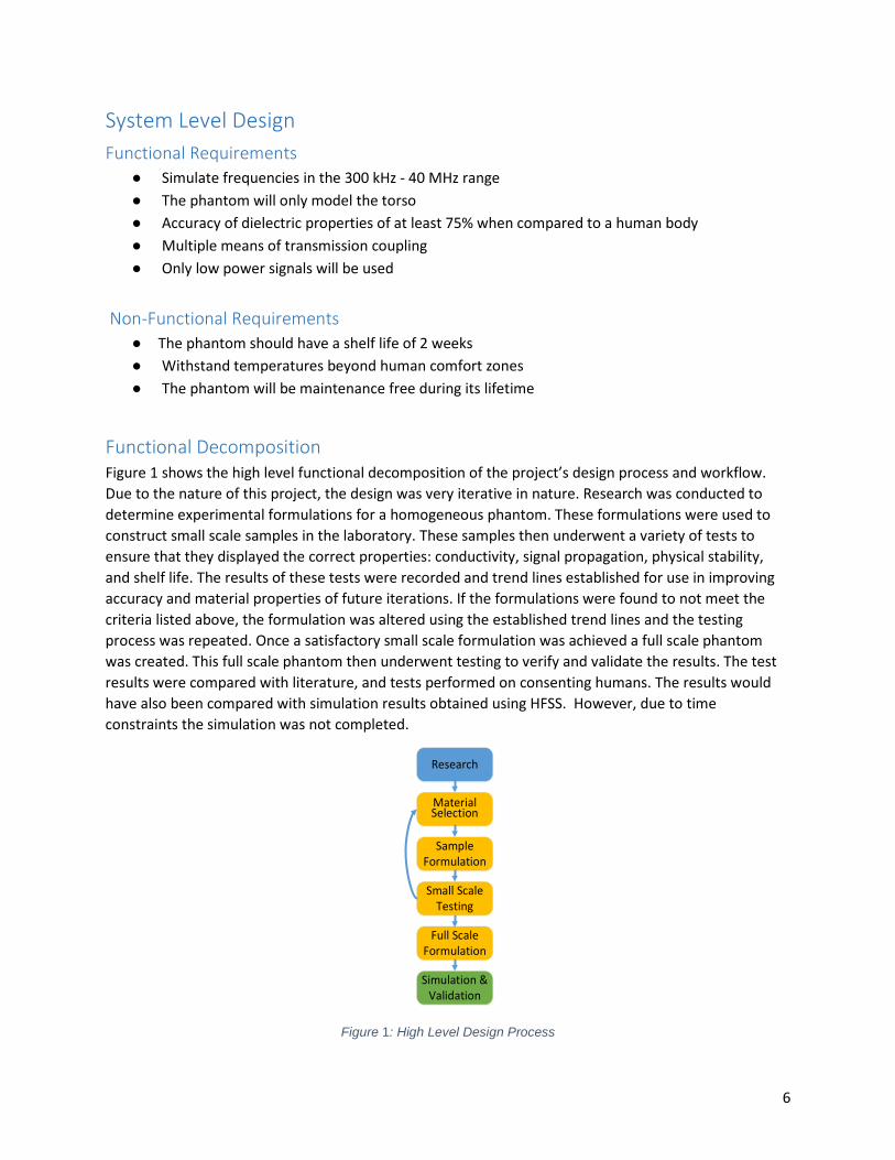
Functional Decomposition Figure 1 shows the high level functional decomposition of the project’s design process and workflow. Due to the nature of this project, the design was very iterative in nature. Research was conducted to determine experimental formulations for a homogeneous phantom. These formulations were used to construct small scale samples in the laboratory. These samples then underwent a variety of tests to ensure that they displayed the correct properties: conductivity, signal propagation, physical stability, and shelf life. The results of these tests were recorded and trend lines established for use in improving accuracy and material properties of future iterations. If the formulations were found to not meet the criteria listed above, the formulation was altered using the established trend lines and the testing process was repeated. Once a satisfactory small scale formulation was achieved a full scale phantom was created. This full scale phantom then underwent testing to verify and validate the results. The test results were compared with literature, and tests performed on consenting humans. The results would have also been compared with simulation results obtained using HFSS. However, due to time constraints the simulation was not completed.

Research

Sample Formulation

Small Scale Testing

Simulation & Validation

Material Selection

Full Scale Formulation

Figure 1: High Level Design Process

7

Formulation Three primary formulations were used during the course of the project. The first formulation tested was gelatin based, the next iteration was a physiological saline encapsulated in a 4 mil poly vinyl chloride bag, and the final iteration was an agar based model. The Agar formulation will be discussed in this section the others can be found in appendix II.

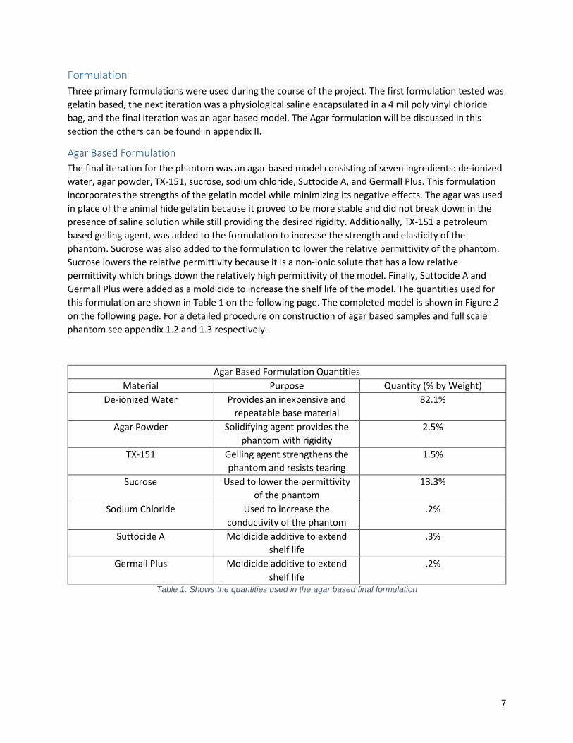
Agar Based Formulation The final iteration for the phantom was an agar based model consisting of seven ingredients: de-ionized water, agar powder, TX-151, sucrose, sodium chloride, Suttocide A, and Germall Plus. This formulation incorporates the strengths of the gelatin model while minimizing its negative effects. The agar was used in place of the animal hide gelatin because it proved to be more stable and did not break down in the presence of saline solution while still providing the desired rigidity. Additionally, TX-151 a petroleum based gelling agent, was added to the formulation to increase the strength and elasticity of the phantom. Sucrose was also added to the formulation to lower the relative permittivity of the phantom. Sucrose lowers the relative permittivity because it is a non-ionic solute that has a low relative permittivity which brings down the relatively high permittivity of the model. Finally, Suttocide A and Germall Plus were added as a moldicide to increase the shelf life of the model. The quantities used for this formulation are shown in Table 1 on the following page. The completed model is shown in Figure 2 on the following page. For a detailed procedure on construction of agar based samples and full scale phantom see appendix 1.2 and 1.3 respectively.

Agar Based Formulation Quantities Material Purpose Quantity (% by Weight)

De-ionized Water Provides an inexpensive and repeatable base material

82.1%

Agar Powder Solidifying agent provides the phantom with rigidity

2.5%

TX-151 Gelling agent strengthens the phantom and resists tearing

1.5%

Sucrose Used to lower the permittivity of the phantom

13.3%

Sodium Chloride Used to increase the conductivity of the phantom

.2%

Suttocide A Moldicide additive to extend shelf life

.3%

Germall Plus Moldicide additive to extend shelf life

.2%

Table 1: Shows the quantities used in the agar based final formulation

8

Figure 2: Completed torso phantom

Computer Simulation Computational Phantom The first step was to obtain a suitable computer model of the human body referred to as a phantom. Dr. George Zubal of Yale University makes his phantom readily available for academic use found at http://noodle.med.yale.edu/zubal/data.htm. The available phantom data is provided in a binary format as a stack of 2-D greyscale images segmented into 39 different tissues. Each pixel’s coloring signifies a different tissue. Each pixel represents a 10x10x10mm3 cubal voxel. The original plan was to simulate a signal propagating through the phantom and use the results to verify the accuracy of the physical model. The simulation would use each tissue’s individual dielectric properties. These properties are available through the Foundation for Research on Information Technologies in Society (IT’IS). Due to time constraints the simulation was not completed..

Alternative phantoms maintained by IT’IS as part of the ‘Virtual Population’ were considered. These phantoms are in a higher resolution at 0.5x0.5x0.5mm3 and segmented into approximately 300 organs and tissues. The high resolution and the number of different tissues would significantly impact the amount of time needed to run a simulation. Thus it was decided to not use these phantoms until we were able simulate the lower resolution phantom.

9

Design Process

Figure 3: Process for converting phantom data and running the simulation.

After finding a suitable phantom a simulation software was chosen. Ansys High Frequency Structural Simulator (HFSS) was chosen due to its availability on campus and at Honeywell. The next step was to convert the model into a HFSS compatible format and setup the simulation and use the results as a target for the physical model.

Phantom Conversion The Zubal model is available in a format where each voxel is specified by an X-Y-Z coordinate followed by the color specifying the tissue. This format could not be imported into HFSS directly. The model format was converted to the common stereolithography (.stl) format. An example can be found in Appendix IV. This format was chosen because HFSS is able to import STL files and the open source software MeshLab is able to manipulate STL files. MeshLab is a 3-D mesh processing software. This software was used to view the data as well as a conversion tool. Before beginning the conversion process we needed to ensure the STL file generated by MeshLab could be successfully imported into HFSS. This is illustrated in Figure 4 below.

10

Figure 4: (Left) Tetrahedral.off in MeshLab. (Right) Tetrahedral.stl in HFSS.

Conversion Process The phantom data was first converted into Object File Format (.off) by the Java code found in Appendix IV. This conversion was necessary to import the data into MeshLab. An example of an .off file encoded in ASCII text is also located in Appendix IV. The coloring was preserved by adding the color at the end of each face definition. In order to convert this data into OFF each cube needed to be specified by its vertices and faces. The vertices were extracted from the center point by adding and subtracting 0.5 from each X, Y, and Z coordinate. This yields all eight of the cube’s vertices. The faces were then defined by the four vertices in a counter clockwise order. This was done because the normal of the face is calculated using the right hand rule.

This process was done first with a single cube, then using MeshLab, converted into STL and then imported into HFSS. This is illustrated in Figure 5 below.

Figure 5: (Left) Cube.off in MeshLab. (Right) Cube.stl in HFSS.

After this was successful it was done with just the head of the model shown in Figure 6 on the following page. This was done because the process of converting and importing the 102,735 voxels comprising the phantom is a resource and time consuming process. It was therefore prudent to ensure this process would be successful with a smaller subset of the data before attempting it with the whole phantom.

12

Figure 6: (Left) Head.off in MeshLab. (Right) Head.stl in HFSS.

Following the successful importation into HFSS this was repeated with the whole phantom shown below in Figure 7.

Figure 7: (Left) Human.off in MeshLab. (Right) Human.stl in HFSS

One challenge that arose during this process was the coloring used to signify which tissue a voxel represents was not preserved following the importation into HFSS.. The process formulated to overcome this obstacle was to separate each organ and convert them individually. However, the first attempt at implementing this showed the geometry was not correctly aligned this is shown in Figure 8 on the following page. The process was repeated to ensure the two tissues were converted identically and yielded the same result. Due to time constraints realigning the geometry was not pursued further. It

13

was decided at this time it would still be useful to have a simulation with a homogenous material defined with the same properties as the target material of the physical model.

Figure 8: Misaligned geometry in HFSS.

Since we decided to use a homogeneous material the complicated geometry used to keep the different tissues separated was no longer needed. Therefore a Poisson surface reconstruction was performed on the phantom which would greatly reduce the size of the file and the amount of time needed to run a simulation. The results were a rough approximation of the outside surface of the phantom shown in Figure 9 below.

Figure 9: (Left) Phantom before reconstruction. (Right) Phantom after reconstruction.

14

Simulation The first simulation ran was a cylinder of seawater. This was done because the conductivity of seawater is known to be 4 S/m thus allowing verifiable simulation results. The simulation was setup with the ends of the cylinder defined as perfect conductors. The cylinder was then enclosed in an air cylinder with two of its faces defined as radiated boundaries. The face in contact with the seawater cylinder was defined as the ground. The length of the cylinder is 8 mm and the radius is 32 mm shown in Figure 10 below. These dimensions are identical to the puck used for testing the conductivity of the various possible materials used for the physical model. Then a frequency sweep was setup from 300 kHz to 40 MHz. Using the equation 𝑅𝑅 = 𝑙𝑙 (𝜎𝜎𝜎𝜎) the conductivity was calculated with the real part of the resulting Z-

matrix. Simulations were ran with the length of seawater cylinder ranging from 8 mm to 2000 mm. This was done due to early errors in the simulation setup the yielded a conductivity of 4 S/m only when R was close to 50Ω. After these errors were corrected these different simulations showed the conductivity to be more consistent. These results are shown in Figures 11-13.

Figure 10: Seawater cylinder encased in a cylinder of air.

Figure 11: L = 29 cm (R = 50.21Ω)

15

Figure 12: L = 0.8 cm.

Figure 13: L = 200 cm.

After the simulations yielded consistent results the sea water cylinder was assigned a new material defined with the same dielectric properties as the target material for the physical model shown in Figure 14 below. The results of the simulation for the puck are shown in Figure 15 on the following page.

Figure 14: Puck material with identical dielectric properties of the physical model material.

16

Figure 15: Simulation results of puck.

At this point the complexity of the geometry was increased. These simulations were setup with a finite conductivity boundaries and wave ports defined at the end of each arm. The resulting electric fields were taken at 21MHz shown in Figure 16 and Figure 17. Unfortunately, neither of these simulations yielded convincing results. The resulting S-parameters were below -275 dB. The material was replaced with a lossless dielectric by setting the conductivity to 0 S/m and the results were in the same range. Thus there was an error in the initial setup. Due to time constraints we were unable to fully investigate and correct the errors.

Figure 16: Simplistic approximation of a human torso.

17

Figure 17: More complex approximation of a human torso.

At this point the reconstructed human phantom was imported into HFSS. A simulation was setup by applying a 21 MHz voltage to a perfect conducting plate touching the top of the head. The resulting electric field is shown below. The simulation for the reconstructed phantom was setup this way because the arms were not separated in the reconstruction process. This is shown in Figure 18 below.

Figure 18: Electric field result from 21MHz signal applied at the top of the head.

18

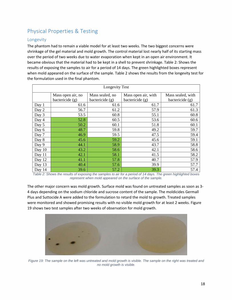
Physical Properties & Testing Longevity The phantom had to remain a viable model for at least two weeks. The two biggest concerns were shrinkage of the gel material and mold growth. The control material lost nearly half of its starting mass over the period of two weeks due to water evaporation when kept in an open air environment. It became obvious that the material had to be kept in a shell to prevent shrinkage. Table 2: Shows the results of exposing the samples to air for a period of 14 days. The green highlighted boxes represent when mold appeared on the surface of the sample. Table 2 shows the results from the longevity test for the formulation used in the final phantom.

Longevity Test

Mass open air, no bactericide (g)

Mass sealed, no bactericide (g)

Mass open air, with bactericide (g)

Mass sealed, with bactericide (g)

Day 1 61.6 61.6 61.7 61.7 Day 2 56.7 61.2 57.9 61.3 Day 3 53.5 60.8 55.1 60.8 Day 4 52.8 60.5 53.6 60.6 Day 5 50.2 60.1 51.8 60.1 Day 6 48.7 59.8 49.2 59.7 Day 7 46.9 59.5 47.5 59.4 Day 8 45.6 59.2 45.6 59.1 Day 9 44.1 58.9 43.7 58.8 Day 10 43.2 58.6 42.1 58.6 Day 11 42.1 58.1 41.5 58.2 Day 12 41.1 57.8 40.7 57.9 Day 13 40.4 57.6 39.9 57.7 Day 14 39.6 57.2 39.3 57.4

Table 2: Shows the results of exposing the samples to air for a period of 14 days. The green highlighted boxes represent when mold appeared on the surface of the sample.

The other major concern was mold growth. Surface mold was found on untreated samples as soon as 3-4 days depending on the sodium chloride and sucrose content of the sample. The moldicides Germall Plus and Suttocide A were added to the formulation to retard the mold to growth. Treated samples were monitored and showed promising results with no visible mold growth for at least 2 weeks. Figure 19 shows two test samples after two weeks of observation for mold growth.

Figure 19: The sample on the left was untreated and mold growth is visible. The sample on the right was treated and

no mold growth is visible.

19

Durability The phantom material had to be hard enough to stand on its own and soft enough to be moldable for a workable amount of time. Multiple iterations of testing led to a formulation that set up hard enough to stand on its own while maintaining the target electrical properties. Unfortunately, the material was susceptible to shrinkage when left in the open air. A hard plastic torso shell was used to solve that problem and add rigidity to the model.

Low Frequency Ohmic Cell The ohmic cell shown in Figure 20 was built for initial conductivity testing of liquid or soft gel solutions at low frequencies. The conductivity was found by filling the ohmic cell with a testing medium and applying a voltage of 6.5 Vpp across the two leads with the function generator. The solution consisted of 500 mL of DI water with varying concentrations of salt by weight. The current that went through the ohmic cell was then measured. The frequency was set from 1 kHz to 3 kHz in steps to measure conductivity at different frequencies. The conductivity was then calculated from the equation σ = l/(R*A) where l is the length between the two electrodes, R is the resistance of the material, and A is the surface area of the electrodes. The resistance was calculated using Ohm's law V = IR. Sample results from ohmic cell testing conducted at 3 KHz are shown in Figure 21.

Figure 20: The ohmic cell used for initial testing is shown above.

20

Figure 21: The plot above shows the data from the ohmic cell testing. The conductivity of the solution increased

linearly as the ratio of NaCl to water was increased.

Saline Model A saline model was the next logical step after completing the ohmic cell and parallel plate capacitor testing. As such, a 0.9% physiological saline model was constructed using 4 mil PVC to simulate human skin. A plastic sealer was purchased to seal the seams of the PVC in order for it to hold the liquid solution. The tubular model was tested at lower frequencies using a function generator to supply the differential input signal while the output was differentially measured with an oscilloscope. The PVC proved to be too resistive as no signal was received. Since the test results were so poor, the saline model was abandoned.

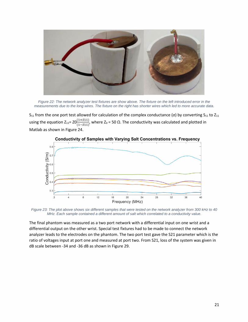
High Frequency Network Analyzer The network analyzer was used to find one and two port S parameter values. The network analyzer had to be calibrated prior to performing tests using an ideal open, ideal short, and a 50 Ω termination for one and two port tests and an ideal through for the two port tests. The one port tests were conducted using the test fixture shown in Figure 23, where the bottom copper plate served as the ground connection and the top copper plate served as the network input.

0

0.2

0.4

0.6

0.8

1

1.2

1.4

1.6

0 0.5 1 1.5 2 2.5 3 3.5

Cond

uctiv

ity (S

/m)

NaCl (g)

Small Scale Ohmic Cell Salt vs Conductivity

21

Figure 22: The network analyzer test fixtures are show above. The fixture on the left introduced error in the

measurements due to the long wires. The fixture on the right has shorter wires which led to more accurate data.

S11 from the one port test allowed for calculation of the complex conductance (σ) by converting S11 to Z11

using the equation Z11= Z0(1+𝑆𝑆11)(1−𝑆𝑆11)

, where Z0 = 50 Ω. The conductivity was calculated and plotted in

Matlab as shown in Figure 24.

Figure 23: The plot above shows six different samples that were tested on the network analyzer from 300 kHz to 40

MHz. Each sample contained a different amount of salt which correlated to a conductivity value.

The final phantom was measured as a two port network with a differential input on one wrist and a differential output on the other wrist. Special test fixtures had to be made to connect the network analyzer leads to the electrodes on the phantom. The two port test gave the S21 parameter which is the ratio of voltages input at port one and measured at port two. From S21, loss of the system was given in dB scale between -34 and -36 dB as shown in Figure 29.

22

Figure 24: The phantom network analyzer test fixture is shown above. Identical test fixtures were used for each wrist

to get the two port parameters.

Matlab Matlab was used to import the S parameter files from the network analyzer and manipulate the data. In order to find the conductivity of the samples, the S values had to be first be converted from the decibels

(S11 dB) scale to the linear magnitude scale (|S11|) using the equation |S| =10𝑆𝑆11(𝑑𝑑𝑑𝑑)

20 . It is important to note that the S11 dB value is divided by 20 because the S parameters are ratios of voltages. The phase angle of the S11 parameter was also considered in σ and was given by the network analyzer in degrees. The complex value of σ was very small compared to the real value and was neglected in the σ calculations. The code used in analysis of S parameter data can be found in appendix IV.

Verification and Validation Small Scale Repeatability The first stage of the validation process was ensuring repeatability of the tuned small-scale sample. To do that five samples were made using the same formulation, and all five were tested using the network analyzer to ensure a repeatable and accurate conductivity was achievable. The results of that test are shown in Figure 26 below. Completion of this test showed a max conductivity of .48 S/m and a minimum conductivity of .41 S/m. The test revealed a maximum percent difference of 4.1% and a maximum percent error of 10.8% when compared with the target conductivity of .46 S/m. The error found at 21 MHz (the IEEE standard for human body networks) was 4.45% which is well within tolerance. From this data the small scale formulation was confirmed to be repeatable and accurate.

23

Figure 25: Small scale repeatability test. Five identical samples were prepared and conductivity was tested.

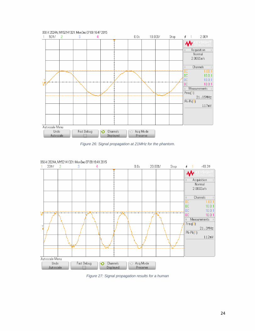
Signal Propagation Test The first verification and validation test the phantom underwent was a signal propagation test. This test utilized a function generator and oscilloscope. In this test a 21 MHz signal was applied to the phantom via galvanic coupling and the signal was received utilizing a galvanically coupled oscilloscope. The received voltage was then compared to the results of the same test being performed on consenting humans. A sample of these test results is shown in Figure 27 and Figure 28 below. The largest percent error in signal propagation found during this test was 19.7% and the smallest percent error in signal propagation was 4.3%. This range of signal propagation differences was determined to be acceptable due to the requirement that the phantom be 25% accurate in signal propagation. Additionally, the signal attenuation was calculated and converted to a log scale to be compared with results received from the network analyzer verification and validation test which will be discussed in the next section.

24

Figure 26: Signal propagation at 21MHz for the phantom.

Figure 27: Signal propagation results for a human

25

Network Analyzer Validation The plot shown in Figure 29 for multiple torso tests on the network analyzer are shown below. The green and yellow signals came from a medical grade electrode and the orange and blues signals came from a research grade electrode. Figure 29 shows four separate tests on the phantom from 300 kHz to 40 MHz. Two of the electrodes were “wet” with conductive gel and the other two electrodes were “dry” or used without any conductive gel. Little variance between the tests was expected since the phantom was modeled as wet skin and the surface of the model is a moist gel. The measured values were mostly constant at -34 for the wet electrodes and -36 dB for the dry electrodes between 300 kHz and 21 MHz with a growing pattern of oscillation above 21 MHz. Data was not collected above 40 MHz and it is unknown whether the oscillations continue to grow or not for higher frequencies.

Figure 28: S21 for multiple torso tests on the network analyzer are shown above. The green and yellow signals came

from a medical grade electrode and the red and blues signals came from research grade electrodes.

The gain listed in literature for similar tests ranges between -50 dB and -10 dB. The measured range of -34 to -36 dB is in the expected range and matches the data collected from the oscilloscope tests shown in Figure 27and Figure 28. The possible sources of the oscillation could come from the calibration of the network analyzer or from instabilities of the material.

Conclusion A physical phantom was designed, developed and constructed in order to match the dielectric properties of the human body. The phantom has signal attenuation accuracy of 75% or greater when compared to the signal attenuation through the human body. In addition to a physical phantom, a computational phantom would have been simulated in HFSS but due to time constraints was not able to be completed. In order to verify and validate our physical phantoms accuracy, the physical phantom would have been compared to the computational phantom’s simulation results. The team was also told that taking measurement of an actual human with the network analyzer was not allowed due to ethical concerns of human testing. Instead documented literature sources and other test means will serve as the verification and validation of the physical phantom. Honeywell will use the physical phantom in order to test body area networks (BAN's) without the risk associated with human subject testing. Since the physical phantom will have a minimum two week shelf life, Honeywell can run multiple test cycles without the phantom degrading.

26

Appendix I Procedures 1.1 Animal Hide Gelatin Test Sample Formulation Purpose

Develop samples to be used for tuning the conductivity of the gelatin based formulation. These sample will be used to determine to perform various tests on. The results of these test will either be accepted as the final formulation or used in developing future formulations.

Materials

1. De-ionized Water (23.5 ⁰C) 2. Animal Hide Gelatin Powder 3. NaCl (Sodium Chloride) 4. Sterile Paper Towels 5. Anti-Bacterial Detergent

Equipment

1. 100mL Graduated Cylinder 2. 10mL Beaker 3. Glass Stir Rod 4. Magnetic Stir Bar 5. Corning PC-420D Hot Plate with Magnetic Stirring 6. Cylindrical Mold measuring 5.08 cm in diameter by 5.08 cm tall 7. Evaporating Dish (3) 8. Mettler Toledo ML Digital Balance 9. Nitrile Gloves 10. Lab Coat 11. Eye Protection

Procedure

1. Thoroughly clean all equipment using soap and de-ionized water. 2. Dry all equipment using sterile paper towels. 3. Using the Graduated Cylinder measure 50 ml of de-ionized water 4. Poor 50 ml of de-ionized water into 100 ml beaker. 5. Add magnetic stir bar to the 100 ml beaker. 6. Place beaker on the stir plate and set the stir plate to 600 RPM. 7. Using and evaporating dish and digital balance weigh the appropriate quantity of Gelatin. 8. Using and evaporating dish and digital balance weigh the appropriate quantity of sodium

chloride. 9. Add the weighed sodium chloride and gelatin to the beaker containing 50ml of de-ionized water. 10. Allow to stir at 600 RPM for 1 min ensure that that Gelatin and sodium chloride has been

thoroughly dissolved. 11. Heat on a 400 ⁰C hot plate while stirring at 600 RPM until the mixture has reached 90 ⁰C. 12. Poor the solution into the cylindrical mold.

27

13. Allow the mixture to set up at room temperature for 6 min prior to removing from the mold.

1.2 Agar Test Sample Formulation Purpose

Develop samples to be used for tuning the conductivity of the agar based formulation. These sample will be used to determine to perform various tests on. The results of these test will either be accepted as the final formulation or used in developing future formulations.

Materials

1. De-ionized Water (23.5 ⁰C) 2. Agar Powder 3. TX-151 4. C12H22011 (Sucrose) 5. NaCl (Sodium Chloride) 6. Sterile Paper Towels 7. Anti-Bacterial Detergent

Equipment

1. 100mL Graduated Cylinder 2. 10mL Beaker 3. Glass Stir Rod 4. Magnetic Stir Bar 5. Corning PC-420D Hot Plate with Magnetic Stirring 6. Cylindrical Mold measuring 5.08 cm in diameter by 5.08 cm tall 7. Evaporating Dish (4) 8. Mettler Toledo ML Digital Balance 9. Nitrile Gloves 10. Lab Coat 11. Eye Protection

Procedure

1. Thoroughly clean all equipment using soap and de-ionized water. 2. Dry all equipment using sterile paper towels. 3. Using the Graduated Cylinder measure 50 ml of de-ionized water 4. Poor 50 ml of de-ionized water into 100 ml beaker. 5. Add magnetic stir bar to the 100 ml beaker. 6. Place beaker on the stir plate and set the stir plate to 600 RPM. 7. Using and evaporating dish and digital balance weigh the appropriate quantity of Agar. 8. Using and evaporating dish and digital balance weigh the appropriate quantity of sodium

chloride. 9. Using and evaporating dish and digital balance weigh the appropriate quantity of sucrose. 10. Using and evaporating dish and digital balance weigh the appropriate quantity of TX-151.

28

11. Add the weighed sodium chloride and agar to the beaker containing 50ml of de-ionized water. 12. Allow to stir at 600 RPM for 1 min ensure that that Agar and sodium chloride has been

thoroughly dissolved. 13. Heat on a 400 ⁰C hot plate while stirring at 600 RPM until the mixture has reached 90 ⁰C 14. Add the weighed TX-151 and sucrose to the de-ionized water, sodium chloride and agar

solution. 15. Set stir plate to 1150 RPM and stir the solution for 30 seconds. 16. Poor the solution into the cylindrical mold 17. Allow the mixture to set up at room temperature for 6 min prior to removing from the mold.

1.3 Agar Full Scale Formulation Purpose

This procedure outlines how the final full scale phantom will be made. The final phantom will require 49 liters of solution.

Materials

1. De-ionized Water (23.5 ⁰C) 2. Agar Powder 3. TX-151 4. C12H22011 (Sucrose) 5. NaCl (Sodium Chloride) 6. Germall Plus 7. Suttocide A 8. Human torso mold 9. Sterile Paper Towels 10. Anti-Bacterial Detergent

Equipment

1. 1 L Graduated Cylinder 2. 600 mL Beaker (6) 3. Glass Stir Rod 4. Magnetic Stir Bar (6) 5. Corning PC-420D Hot Plate with Magnetic Stirring (6) 6. Evaporating Dish (20) 7. Mettler Toledo ML Digital Balance (4) 8. Nitrile Gloves 9. Lab Coat 10. Eye Protection 11. Electric Drill 12. Paint Stirrer

Procedure

1. Thoroughly clean all equipment using soap and de-ionized water.

29

2. Dry all equipment using sterile paper towels. 3. Using the Graduated Cylinder measure 500 ml of de-ionized water 4. Poor 500 ml of de-ionized water into 600 ml beaker. 5. Add magnetic stir bar to the 600 ml beaker. 6. Place beaker on the stir plate and set the stir plate to 600 RPM. 7. Using and evaporating dish and digital balance weigh the appropriate quantity of Agar.

Quantities are shown in the table in the formulation section. 8. Using and evaporating dish and digital balance weigh the appropriate quantity of sodium

chloride. Quantities are shown in the table in the formulation section. 9. Using and evaporating dish and digital balance weigh the appropriate quantity of sucrose.

Quantities are shown in the table in the formulation section. 10. Using and evaporating dish and digital balance weigh the appropriate quantity of TX-151.

Quantities are shown in the table in the formulation section. 11. Add the weighed sodium chloride and agar to the beaker containing 500 ml of de-ionized water. 12. Allow to stir at 600 RPM for 1 min ensure that that Agar and sodium chloride has been

thoroughly dissolved. 13. Heat on a 400 ⁰C hot plate while stirring at 600 RPM until the mixture has reached 90 ⁰C 14. Add the weighed TX-151 and sucrose to the de-ionized water, sodium chloride and agar

solution. 15. Stir using drill and paint stirrer 16. Poor the solution into the human torso mold

Formulation

Gelatin Based Formulation Quantities Material Purpose Quantity (% by Weight)

De-ionized Water Provides an inexpensive and repeatable base material

82.1%

Agar Powder Solidifying agent provides the phantom with rigidity

2.5%

TX-151 Gelling agent strengthens the phantom and resists tearing

1.5%

Sucrose Used to lower the permittivity of the phantom

13.3%

Sodium Chloride Used to increase the conductivity of the phantom

.2%

Suttocide A Moldicide additive to extend shelf life

.3%

Germall Plus Moldicide additive to extend shelf life

.2%

30

1.4 TX-151 Formulation Purpose

Develop samples to be used for baseline conductivity and permittivity testing. These sample will be used to determine the feasibility of the formulation. If the formulation is found feasible further analysis will be performed and trend lines developed for further design.

Materials

1. De-ionized Water (23.5 ⁰C) 2. TX-151 3. C12H22011 (Sucrose) 4. NaCl (Sodium Chloride) 5. Sterile Paper Towels 6. Anti-Bacterial Detergent

Equipment

1. 100mL Graduated Cylinder 2. 10mL Beaker 3. Glass Stir Rod 4. Magnetic Stir Bar 5. Corning PC-410D Stir Plate 6. Cylindrical Mold measuring 5.08 cm in diameter by 5.08 cm tall 7. Evaporating Dish (3) 8. Mettler Toledo ML Digital Balance 9. Nitrile Gloves 10. Lab Coat 11. Eye Protection

Procedure

1. Thoroughly clean all equipment using soap and de-ionized water. 2. Dry all equipment using sterile paper towels. 3. Using the Graduated Cylinder measure 50 ml of de-ionized water 4. Poor 50 ml of de-ionized water into 100 ml beaker. 5. Add magnetic stir bar to the 100 ml beaker. 6. Place beaker on the stir plate and set the stir plate to 600 RPM. 7. Using and evaporating dish and digital balance weigh the appropriate quantity of sodium

chloride. Quantities can be found in the table in the formulation section. 8. Using and evaporating dish and digital balance weigh the appropriate quantity of sucrose.

Quantities can be found in the table in the formulation section 9. Using and evaporating dish and digital balance weigh the appropriate quantity of TX-151. 10. Add the weighed sodium chloride and sucrose to the beaker containing 50ml of de-ionized

water. 11. Allow to stir at 600 RPM for 1 min ensure that that sucrose and sodium chloride has been

thoroughly dissolved.

31

12. Add the weighed TX-151 to the sodium chloride, sucrose, and de-ionized water solution. 13. Set stir plate to 1150 RPM and stir the sodium chloride, sucrose, and de-ionized water solution

for 30 seconds. 14. Poor the sodium chloride, sucrose, TX-151, and de-ionized water solution into the cylindrical

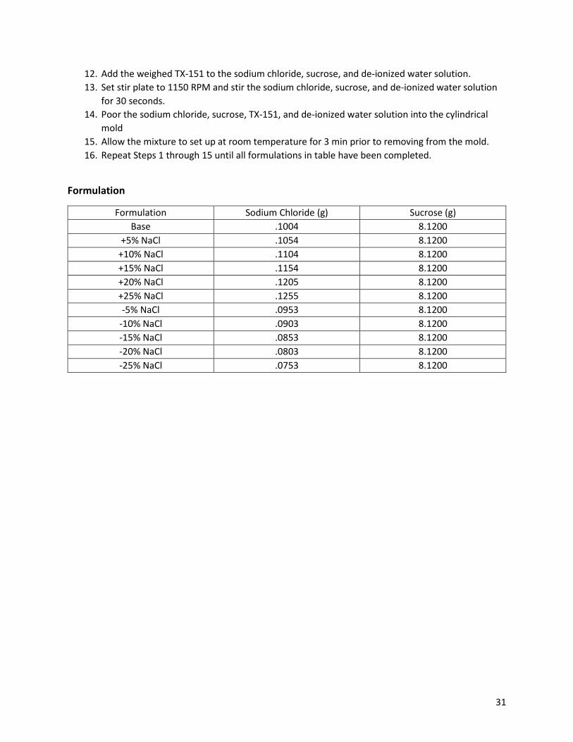
mold 15. Allow the mixture to set up at room temperature for 3 min prior to removing from the mold. 16. Repeat Steps 1 through 15 until all formulations in table have been completed.

Formulation

Formulation Sodium Chloride (g) Sucrose (g) Base .1004 8.1200

+5% NaCl .1054 8.1200 +10% NaCl .1104 8.1200 +15% NaCl .1154 8.1200 +20% NaCl .1205 8.1200 +25% NaCl .1255 8.1200 -5% NaCl .0953 8.1200

-10% NaCl .0903 8.1200 -15% NaCl .0853 8.1200 -20% NaCl .0803 8.1200 -25% NaCl .0753 8.1200

32

Appendix II Alternative designs Gelatin Based Phantom Formulation The first iteration of the physical phantom was based around gelatin this material was chosen due to its accessibility, cost, and ease of use. The initial formulation consisted of three ingredients: de-ionized was three ingredients: de-ionized water, animal hide gelatin, and sodium chloride. The quantities of materials used in this formulation are shown in the table below, for a detailed procedure see appendix 1.1. We found this formulation to be adequate in producing the desired conductivity results of .46 S/m. unfortunately while performing longevity test it was found that this formulation breaks down in the presence of saline solution and is susceptible to molding. Due to these shortcomings the formulation was abandoned.

Gelatin Based Formulation Quantities Material Purpose Quantity (% by Weight)

De-ionized Water Provides an inexpensive and repeatable base material

97.4%

Gelatin Solidifying agent 2.4% Sodium Chloride Conductivity Control .2%

Physiological Saline phantom The second iteration consisted of bags made of various plastics filled with a mixture of 9% physiological saline. This iteration was chosen due to the similar properties physiological saline shares with human body fluid and the fact that the body contains a high percentage of body fluid by volume. Testing showed the physiological saline to have a conductivity of 1.5 S/m which is comparable body fluids conductivity. Testing was also performed to select the best plastic sheeting for bag material which was found to be poly vinyl chloride (PVC). This formulation showed initial promise due to its relative ease of construction, simplicity, repeatability, and longevity. However, quickly after beginning electrical testing it became apparent that though transmission across the bags was possible it was not simulating a human. This is largely attributed to the high resistance of the PVC sheeting the high conductivity of the fluid compared to the average conductivity of the body.

33

Appendix III Operation Manual Computer Simulation

1. Compile and run the Java code in Appendix IV with two command line arguments “HUGO_stand_10mm.vox” and “humanCubeDemo.off”.

2. Open MeshLab and select File -> Import Mesh and select the newly created file “humanCubeDemo.off”.

3. In MeshLab select Filters -> Remeshing, Simplification and Reconstruction -> Surface Reconstruction: Poisson.

4. Set Octree Depth to 6, Solver Divide to 6, Samples per Node to 1, and Surface offsetting to 1 then select Apply.

5. Select File -> Export Mesh As then in the Files of type drop down menu select Stereolithography (*.stl).

6. Name the file “humanCubeDemo.stl” and select Save. 7. Open HFSS and create a new project. 8. Select Project -> Insert HFSS Design. 9. Select Modeler -> Import File and locate the newly created STL file and select Open. 10. At this step HFSS takes some time to read in the STL file. 11. After the model has finished rendering, select HFSS -> Solution Type and ensure Modal and

Network Analysis are selected. 12. Select HFSS -> Analysis Setup -> Add Solution Setup. 13. Set solution frequency to 21 MHz and select OK. 14. Select Draw -> Rectangle and at the bottom of the screen enter 0 for the X-coordinate, 0 for the

Y-coordinate and 0.1 for the Z-coordinate. 15. Then enter in 6 for X displacement, 4 for Y displacement and 0 for Z displacement. 16. Select Edit -> Select -> Faces. 17. Select Edit -> Select -> By Name then locate the rectangle just created. 18. Select HFSS -> Boundaries -> Assign -> Perfect E. 19. Select Edit -> Select -> By Name -> bounding_box1. (This box is imported with the human

phantom.) 20. Select every face except the one located at the phantom’s face while holding CTRL. 21. Select HFSS -> Boundaries -> Assign -> Radiation. 22. Select Edit -> Select -> By Name -> bounding_box1, and select the face located at the phantom’s

feet. 23. Select HFSS -> Boundaries -> Assign -> Perfect E, then select the Infinite Ground Plane check box

and select OK. 24. Right click on bounding_box1 located in the design tree and select Edit -> Arrange -> Move and

enter 0 for the X-coordinate, 0 for the Y-coordinate and -9.4 for the Z-coordinate. 25. Select Edit -> Select -> By Name -> Rectangle1. 26. Select HFSS -> Excitations -> Voltage then specify the E-Field direction and select OK. 27. Right click on bounding_box1 in the design tree and select Assign Materials. 28. Change the material to “air”. 29. Right click on STL in the design tree and select Assign Materials then select Add Material. 30. Name the new material “Human”.

34

31. Change Relative Permittivity to 68.0089. 32. Change Bulk Conductivity to 0.46 and select Validate Material then OK. 33. Select HFSS -> Validation Check and ensure the simulation setup is validated. 34. Select HFSS -> Analyze All. 35. After the simulation is completed select STL from the design tree and select Fields -> Plot Fields

-> E -> Mag_E to plot the electric field distribution inside the phantom. 36. By clicking the legend the field plot scale and coloring can be adjusted.

35

Appendix IV Code Network Analyzer Data Analysis Code clear all close all length = .0072; surface = 0.032^2*pi; Z0 = 50; Y0 = 1/Z0; count = 0; %Flag is set to 1 after first file read so only the header comments are %deleted. Flag = inputdlg('Has this code been run before? Enter 1 for Yes, 0 for No.'); if str2num(Flag1) == 0 for i = 1:14 FileToRewrite = ['A' num2str(i) '.S1P']; % phase 1 : read the ith S1P file fid = fopen(FileToRewrite,'r'); TextDat = textscan(fid,'%s','delimiter','\n'); fclose(fid); % phase 2 : just take from the 4th line (3 headers) until the end-3 % (3 footers) NewTextDat = TextDat1(5+1:end); % phase 3 : rewrite the file with the new data fid = fopen(FileToRewrite,'wt'); fprintf(fid,'Freq \tdB \tPhase\n'); fprintf(fid,'%s\n',NewTextDat:); %scan data for tabs and add comma %M = [M fscanf(fid, '\t')]; fclose(fid); %Flag = 1; end for i = 1:14 FileToRewrite = ['B' num2str(i) '.S1P']; % phase 1 : read the ith S1P file fid = fopen(FileToRewrite,'r'); TextDat = textscan(fid,'%s','delimiter','\n'); fclose(fid); % phase 2 : just take from the 4th line (3 headers) until the end-3 % (3 footers) NewTextDat = TextDat1(5+1:end); % phase 3 : rewrite the file with the new data fid = fopen(FileToRewrite,'wt'); fprintf(fid,'Freq \tdB \tPhase\n'); fprintf(fid,'%s\n',NewTextDat:); %scan data for tabs and add comma %M = [M fscanf(fid, '\t')]; fclose(fid); %Flag = 1; end end

36

%X= struct('Freq',tdfread('A1.S1P','\t'),'Db',tdfread('A1.S1P','\t'),'Phase',); %X = tdfread('A1.S1P','\t') %Read the csv files M = []; for i=1:14 M = [M tdfread(strcat('A', num2str(i),'.S1P'))]; count = count +1; end for i=1:14 M = [M tdfread(strcat('B', num2str(i),'.S1P'))]; count = count + 1; end %Process non-uniformly named files. These files must manipulated manually %prior to using this code. Delete the first 5 lines of code. Then set %the top line as "Freq" tab "dB" tab "Phase". M = [M tdfread(strcat('PLASTIC.S1P'))]; count = count + 1; M = [M tdfread(strcat('SHORT.S1P'))]; count = count + 1; M = [M tdfread(strcat('OPEN.S1P'))]; count = count + 1; %s11 = 0.254*exp(1i*-178.875/180*pi); %Find S parameters. S parameters from the Network Analyzer are given in dB %and must be converted. The theta value must be in radians. %Find the Z and Y parameters from the S parameter. S = []; Y = []; Z = []; for i=1:count S = [S 10.^(M(i).dB/20).*exp(1i*M(i).Phase/180*pi)]; Y = [Y Y0*(1-S(:,i))./(1+S(:,i))]; Z = [Z Z0*(1+S(:,i))./(1-S(:,i))]; end %Sigma = G*lenth/Surface area Roe = real(Z).*(surface/length); Sigma = 1./Roe; %Plot Sigma values for all samples on one graph plot(Sigma); hold on title('Sigma'); xlabel('Sample'); ylabel('Resistivity') %axis([1 501 0 1.5]); %figure

37

hold off

Code for Data Conversion package voxel_test; import java.io.IOException; public class byteMain public static void main(String[] args) throws IOException ByteToOFF off; if(args.length == 2) off = new ByteToOFF(args[0], args[1]); else off = new ByteToOFF(); off.process();

package voxel_test; import java.io.*; import java.util.ArrayList; import java.util.Scanner; public class ByteToOFF private String fileName = "HUGO_stand_10mm.vox"; private String outputFile = "humanCube.off"; static int x_size = 60; static int y_size = 35; static int z_size = 190; static int numCubes = 0; ArrayList<Vertex> vertices = new ArrayList<>(); ArrayList<Face> faces = new ArrayList<>(); public ByteToOFF(String fName, String outFile) fileName = fName; outputFile = outFile; public ByteToOFF() super(); public void process() throws IOException int[] vertex = new int[8]; for(int j = 0; j < 8; j++) vertex[j] = j; FileWriter out = new FileWriter(outputFile); out.write("OFF\n"); processFile();

38

out.write(vertices.size() + " " + faces.size() + " 0\n"); for(int i = 0; i < vertices.size(); i ++) out.write(vertices.get(i).toString() + "\n"); for(int k = 0; k < faces.size(); k++) out.write(faces.get(k).toString() + "\n"); out.close(); System.out.println(numCubes); public void processFile() throws IOException try(FileInputStream in = new FileInputStream(fileName)) BufferedReader br = new BufferedReader(new InputStreamReader(in, "UTF-8")); String line = null; while((line = br.readLine()) != null) if(processLine(line) == 1) break; in.close(); br.close(); public int processLine(String line) Scanner scan = new Scanner(line); scan.useDelimiter(" "); int x = scan.nextInt(); int y = scan.nextInt(); int z = scan.nextInt(); int value = 0; if(scan.hasNextInt()) value = scan.nextInt(); Vertex[] cubeV = new Vertex[8]; int[] v = new int[8]; Face[] cubeF = new Face[6]; /* Code used to separate model parts and tissues. if(z == 24) scan.close(); return 1; else if(value != 5) scan.close(); return 0; */ numCubes++; //The below code removes any duplicated vertices shared between two adjacent voxels. for(int i = 0; i < 8; i++) cubeV[i] = new Vertex(getV(x,y,z,i)); for(int i = 0; i < 8; i++) if(vertices.contains(cubeV[i]))

39

v[i] = vertices.indexOf(cubeV[i]); else v[i] = vertices.size(); vertices.add(cubeV[i]); cubeF[0] = new Face(v[0], v[1], v[3], v[2], value); cubeF[1] = new Face(v[2], v[3], v[5], v[4], value); cubeF[2] = new Face(v[4], v[5], v[7], v[6], value); cubeF[3] = new Face(v[6], v[7], v[1], v[0], value); cubeF[4] = new Face(v[1], v[7], v[5], v[3], value); cubeF[5] = new Face(v[6], v[0], v[2], v[4], value); for(int i = 0; i < 6; i++) //if(!faces.contains(cubeF[i])) faces.add(cubeF[i]); // System.out.println(numCubes); scan.close(); return 0; public double[] getV(int x, int y, int z, int v) switch (v) case 0: return getV0(x,y,z); case 1: return getV1(x,y,z); case 2: return getV2(x,y,z); case 3: return getV3(x,y,z); case 4: return getV4(x,y,z); case 5: return getV5(x,y,z); case 6: return getV6(x,y,z); default: return getV7(x,y,z); public double[] getV0(int x, int y, int z) double v0x = x - 0.5; double v0y = y - 0.5; double v0z = z + 0.5; double[] arr = new double[3]; arr[0] = v0x; arr[1] = v0y; arr[2] = v0z; return arr; public double[] getV1(int x, int y, int z) double v0x = x + 0.5; double v0y = y - 0.5; double v0z = z + 0.5; double[] arr = new double[3];

40

arr[0] = v0x; arr[1] = v0y; arr[2] = v0z; return arr; public double[] getV2(int x, int y, int z) double v0x = x - 0.5; double v0y = y + 0.5; double v0z = z + 0.5; double[] arr = new double[3]; arr[0] = v0x; arr[1] = v0y; arr[2] = v0z; return arr; public double[] getV3(int x, int y, int z) double v0x = x + 0.5; double v0y = y + 0.5; double v0z = z + 0.5; double[] arr = new double[3]; arr[0] = v0x; arr[1] = v0y; arr[2] = v0z; return arr; public double[] getV4(int x, int y, int z) double v0x = x - 0.5; double v0y = y + 0.5; double v0z = z - 0.5; double[] arr = new double[3]; arr[0] = v0x; arr[1] = v0y; arr[2] = v0z; return arr; public double[] getV5(int x, int y, int z) double v0x = x + 0.5; double v0y = y + 0.5; double v0z = z - 0.5; double[] arr = new double[3]; arr[0] = v0x; arr[1] = v0y; arr[2] = v0z; return arr; public double[] getV6(int x, int y, int z) double v0x = x - 0.5; double v0y = y - 0.5; double v0z = z - 0.5; double[] arr = new double[3]; arr[0] = v0x; arr[1] = v0y; arr[2] = v0z; return arr; public double[] getV7(int x, int y, int z) double v0x = x + 0.5;

41

double v0y = y - 0.5; double v0z = z - 0.5; double[] arr = new double[3]; arr[0] = v0x; arr[1] = v0y; arr[2] = v0z; return arr; package voxel_test; public class Face int vertex1; int vertex2; int vertex3; int vertex4; int color; public Face(int v1, int v2, int v3, int v4, int c) vertex1 = v1; vertex2 = v2; vertex3 = v3; vertex4 = v4; color = c; @Override public boolean equals(Object obj) if (this == obj) return true; if (obj == null) return false; if (getClass() != obj.getClass()) return false; Face other = (Face) obj; if (color != other.color) return false; if (vertex1 != other.vertex1) return false; if (vertex2 != other.vertex2) return false; if (vertex3 != other.vertex3) return false; if (vertex4 != other.vertex4) return false; return true; @Override

public String toString() if(color != 0) return "4 " + vertex1 + " " + vertex2 + " " + vertex3 + " " + vertex4 + " " + color; else

42

return "4 " + vertex1 + " " + vertex2 + " " + vertex3 + " " + vertex4; public int getVertex1() return vertex1; public void setVertex1(int vertex1) this.vertex1 = vertex1; public int getVertex2() return vertex2; public void setVertex2(int vertex2) this.vertex2 = vertex2; public int getVertex3() return vertex3; public void setVertex3(int vertex3) this.vertex3 = vertex3; public int getColor() return color; public void setColor(int color) this.color = color;

package voxel_test; public class Vertex double x_coord; double y_coord; double z_coord; public Vertex(double[] arr) x_coord = arr[0]; y_coord = arr[1]; z_coord = arr[2]; public double getX_coord() return x_coord; public double getY_coord()

43

return y_coord; public double getZ_coord() return z_coord; @Override public boolean equals(Object obj) if (this == obj) return true; if (obj == null) return false; if (getClass() != obj.getClass()) return false; Vertex other = (Vertex) obj; if (Double.doubleToLongBits(x_coord) != Double.doubleToLongBits(other.x_coord)) return false; if (Double.doubleToLongBits(y_coord) != Double.doubleToLongBits(other.y_coord)) return false; if (Double.doubleToLongBits(z_coord) != Double.doubleToLongBits(other.z_coord)) return false; return true; @Override public String toString() return x_coord + " " + y_coord + " " + z_coord;

Code Explanation

Figure 29: Orientation of vertex numbering for cubal voxels.

This numbering is identical to how the vertices are numbered in the above code. The code reads the XYZ coordinate from the input file which is interpreted as the center of the cube. From here the code calculates vertex 0 by subtracting 0.5 from the X-coordinate, then subtracting 0.5 from the Y-coordinate and then adding 0.5 to the Z-coordinate. The reason 0.5 is added and subtracted to each individual

44

coordinate is because each voxel is a 1x1x1 cube with a resolution of 10mm. The Cube.off file shown below was used to compare against the output given an input of 0 0 0. After the vertices are calculated for a voxel, each vertex is tested against the current list of vertices to prevent duplicates being written to the output file. This test was done using ArrayList’s contains method. Because the contains method uses an object’s equals method, the vertices and faces were encapsulated in objects. Then by implementing a toString method for the two objects the list of vertices could be iterated through and written to the output file followed by the list of the faces.

File Format Examples Example Input File The first number represents the X-coordinate, the second number represents the Y-coordinate, and the third number represents the Z-coordinate. The fourth number is the 8-bit greyscale color signifying the tissue type.

29 14 2 143 30 14 2 143 28 15 2 5 29 15 2 17 30 15 2 111 31 15 2 5 32 15 2 143 27 16 2 143 28 16 2 111

Cube.off Produced using the above Java code. The faces are defined first by the number of vertices and then by their vertices in a counter clockwise direction. The vertices are selected by their zero indexed order of appearance in the file. The first vertex is vertex 0, the second vertex is vertex 1 and so on.

OFF 8 6 0 -0.500000 -0.500000 0.500000 0.500000 -0.500000 0.500000 -0.500000 0.500000 0.500000 0.500000 0.500000 0.500000 -0.500000 0.500000 -0.500000 0.500000 0.500000 -0.500000 -0.500000 -0.500000 -0.500000 0.500000 -0.500000 -0.500000 4 0 1 3 2 4 2 3 5 4 4 4 5 7 6 4 6 7 1 0 4 1 7 5 3 4 6 0 2 4

45

Cube.stl Produced using MeshLab.

solid STL generated by MeshLab facet normal 5.000000e-001 -7.071068e-001 5.000000e-001 outer loop vertex -3.535534e-001 -7.071068e-001 3.535534e-001 vertex 3.535534e-001 -7.071068e-001 -3.535534e-001 vertex 8.535534e-001 0.000000e+000 1.464466e-001 endloop endfacet facet normal 5.000000e-001 -7.071068e-001 5.000001e-001 outer loop vertex -3.535534e-001 -7.071068e-001 3.535534e-001 vertex 8.535534e-001 0.000000e+000 1.464466e-001 vertex 1.464466e-001 0.000000e+000 8.535534e-001 endloop endfacet facet normal 5.000000e-001 7.071068e-001 5.000000e-001 outer loop vertex 1.464466e-001 0.000000e+000 8.535534e-001 vertex 8.535534e-001 0.000000e+000 1.464466e-001 vertex 3.535534e-001 7.071068e-001 -3.535534e-001 endloop endfacet facet normal 5.000001e-001 7.071068e-001 5.000000e-001 outer loop vertex 1.464466e-001 0.000000e+000 8.535534e-001 vertex 3.535534e-001 7.071068e-001 -3.535534e-001 vertex -3.535534e-001 7.071068e-001 3.535534e-001 endloop endfacet facet normal -5.000000e-001 7.071068e-001 -5.000000e-001 outer loop vertex -3.535534e-001 7.071068e-001 3.535534e-001 vertex 3.535534e-001 7.071068e-001 -3.535534e-001 vertex -1.464466e-001 0.000000e+000 -8.535534e-001 endloop endfacet facet normal -5.000001e-001 7.071068e-001 -5.000000e-001 outer loop vertex -3.535534e-001 7.071068e-001 3.535534e-001 vertex -1.464466e-001 0.000000e+000 -8.535534e-001 vertex -8.535534e-001 0.000000e+000 -1.464466e-001 endloop endfacet facet normal -5.000000e-001 -7.071068e-001 -5.000000e-001 outer loop vertex -8.535534e-001 0.000000e+000 -1.464466e-001 vertex -1.464466e-001 0.000000e+000 -8.535534e-001 vertex 3.535534e-001 -7.071068e-001 -3.535534e-001 endloop endfacet facet normal -5.000000e-001 -7.071068e-001 -5.000001e-001 outer loop vertex -8.535534e-001 0.000000e+000 -1.464466e-001

46

vertex 3.535534e-001 -7.071068e-001 -3.535534e-001 vertex -3.535534e-001 -7.071068e-001 3.535534e-001 endloop endfacet facet normal 7.071068e-001 0.000000e+000 -7.071068e-001 outer loop vertex 3.535534e-001 -7.071068e-001 -3.535534e-001 vertex -1.464466e-001 0.000000e+000 -8.535534e-001 vertex 3.535534e-001 7.071068e-001 -3.535534e-001 endloop endfacet facet normal 7.071068e-001 0.000000e+000 -7.071068e-001 outer loop vertex 3.535534e-001 -7.071068e-001 -3.535534e-001 vertex 3.535534e-001 7.071068e-001 -3.535534e-001 vertex 8.535534e-001 0.000000e+000 1.464466e-001 endloop endfacet facet normal -7.071068e-001 0.000000e+000 7.071068e-001 outer loop vertex -8.535534e-001 0.000000e+000 -1.464466e-001 vertex -3.535534e-001 -7.071068e-001 3.535534e-001 vertex 1.464466e-001 0.000000e+000 8.535534e-001 endloop endfacet facet normal -7.071068e-001 0.000000e+000 7.071068e-001 outer loop vertex -8.535534e-001 0.000000e+000 -1.464466e-001 vertex 1.464466e-001 0.000000e+000 8.535534e-001 vertex -3.535534e-001 7.071068e-001 3.535534e-001 endloop endfacet endsolid vcg

47

References [1]I. Zivkovic, C. Wandrey and B. Bogicevic, 'ALGINATE BEADS AND EPOXY RESIN COMPOSITES AS CANDIDATES FOR MICROWAVE ABSORBERS', PIER C, vol. 28, pp. 127-142, 2012.

[2]I. Zivkovic, R. Mahou, K. Scheffler and C. Wandrey, 'CANDIDATE FOR TISSUE MIMICKING MATERIAL MADE OF AN EPOXY MATRIX LOADED WITH ALGINATE MICROSPHERES', PIER C, vol. 41, pp. 227-238, 2013.

[3]M. Lazebnik, E. Madsen, G. Frank and S. Hagness, 'Tissue-mimicking phantom materials for narrowband and ultrawideband microwave applications', Physics in Medicine and Biology, vol. 50, no. 18, pp. 4245-4258, 2005.

[4]T. Oh, H. Koo, K. Lee, S. Kim, J. Lee, S. Kim, J. Seo and E. Woo, 'Validation of a multi-frequency electrical impedance tomography (mfEIT) system KHU Mark1: impedance spectroscopy and time-difference imaging', Physiol. Meas., vol. 29, no. 3, pp. 295-307, 2008.

[5]M. Hagmann, R. Levin, L. Calloway, A. Osborn and K. Foster, 'Muscle-equivalent phantom materials for 10-100 MHz', IEEE Transactions on Microwave Theory and Techniques, vol. 40, no. 4, pp. 760-762, 1992.

[6]T. Yilmaz, R. Foster and Y. Hao, 'Broadband Tissue Mimicking Phantoms and a Patch Resonator for Evaluating Noninvasive Monitoring of Blood Glucose Levels', IEEE Trans. Antennas Propagat., vol. 62, no. 6, pp. 3064-3075, 2014.

[7]C. Chou, G. Chen, A. Guy and K. Luk, 'Formulas for preparing phantom muscle tissue at various radiofrequencies', Bioelectromagnetics, vol. 5, no. 4, pp. 435-441, 1984.

[8]T. Yamamoto, K. Sano, K. Koshiji, X. Chen, S. Yang, M. Abe and A. Fukuda, 'Development of electromagnetic phantom at low-frequency band', 35th Annual International Conference of the IEEE EMBS, pp. 1887-1890, 2013.

[9]H. Velez, A. Vera and L. Leija, 'Use of Parallel Plates Measurement Method for Designing and Construction of a Measurement System of Measuring Permittivity in Phantoms in 40Hz to 11OMHz Frequencies Range', 2004 I st International Conference on Electrical and Electronics Engineering, pp. 499-504, 2004.

[10]J. Clarys, A. Martin and D. Drinkwater, 'Gross Tissue Weights in the Human Body By Cadaver Dissection', Human Biology, vol. 56, , no. 3, pp. 459-473, 1984.

[11]M. Lazebnik, E. Madsen, G. Frank and S. Hagness, 'Tissue-mimicking phantom materials for narrowband and ultrawideband microwave applications', Physics in Medicine and Biology, vol. 50, no. 18, pp. 4245-4258, 2005.

[12]J. Dardenne, S. Valette, N. Siauve, N. Burais and R. Prost, 'Variational tetrahedral mesh generation from discrete volume data', The Visual Computer, vol. 25, no. 5-7, pp. 401-410, 2009.

[13]M. Wegmueller, M. Oberle, N. Felber, N. Kuster and W. Fichtner, 'Signal Transmission by Galvanic Coupling Through the Human Body', IEEE Trans. Instrum. Meas., vol. 59, no. 4, pp. 963-969, 2010.

48

[14]K. Hachisuka, A. Nakata, T. Takeda, Y. Terauchi, K. Shiba, K. Sasaki, H. Hosaka and K. Itao, 'DEVELOPMENT AND PERFORMANCE ANALYSIS OF AN INTRA-BODY COMMUNICATION DEVICE', The 12th International Conference on Solid State Sensors, Actuators and Microsystems, pp. 1722-1725, 2003.

[15]V. De Santis, P. Beeckman, D. Lampasi and M. Feliziani, 'Assessment of Human Body Impedance for Safety Requirements Against Contact Currents for Frequencies up to 110 MHz', IEEE Transactions on Biomedical Engineering, vol. 58, no. 2, pp. 390-396, 2011.

[16]B. Kibret, M. Seyedi, D. Lai and M. Faulkner, 'Investigation of Galvanic-Coupled Intrabody Communication Using the Human Body Circuit Model', IEEE Journal of Biomedical and Health Informatics, vol. 18, no. 4, pp. 1196-1206, 2014.

[17]T. Ogasawara, A. Sasaki, K. Fujii and H. Morimura, 'Human Body Communication Based on Magnetic Coupling', IEEE Trans. Antennas Propagat., vol. 62, no. 2, pp. 804-813, 2014.

[18]M. Wegmueller, A. Kuhn, J. Froehlich, M. Oberle, N. Felber, N. Kuster and W. Fichtner, 'An Attempt to Model the Human Body as a Communication Channel', IEEE Transactions on Biomedical Engineering, vol. 54, no. 10, pp. 1851-1857, 2007.

[19]S. Gabriel, R. Lau and C. Gabriel, 'The Dielectric Properties of Biological Tissues: II. Measurements in the frequency range 10 Hz to 20 GHz', Physics in Medicine and Biology, vol. 41, no. 11, pp. 2251-2269, 1996.

[20]C. Furse, D. Christensen and C. Durney, Basic Introduction to Bioelectromagnetics. Boca Raton, FL: CRC Press, 2009.

[21]A. Polimeridis, J. Villena, L. Daniel and J. White, 'Stable FFT-JVIE solvers for fast analysis of highly inhomogeneous dielectric objects', Journal of Computational Physics, vol. 269, pp. 280-296, 2014.

[22]A. Christ, W. Kainz, E. Hahn, K. Honegger, M. Zefferer, E. Neufeld, W. Rascher, R. Janka, W. Bautz, J. Chen, B. Kiefer, P. Schmitt, H. Hollenbach, J. Shen, M. Oberle, D. Szczerba, A. Kam, J. Guag and N. Kuster, 'The Virtual Family—development of surface-based anatomical models of two adults and two children for dosimetric simulations', Physics in Medicine and Biology, vol. 55, no. 2, pp. N23-N38, 2009.

[23]H. Kato and T. Ishida, 'Development of an agar phantom adaptable for simulation of various tissues in the range 5-40 MHz.', Physics in Medicine and Biology, vol. 32, no. 2, pp. 221-226, 1987.

[24]I.G. Zubal, C.R Harrell, E.O Smith, Z. Rattner, G. Gindi and P.B. Hoffer, ‘Computerized three-dimensional segmented human anatomy’, Medical Physics, vol. 21, no. 2, pp 299-302, 1994.

[25] Hasgall PA, Di Gennaro F, Baumgartner C, Neufeld E, Gosselin MC, Payne D, Klingenböck A, Kuster N, “IT’IS Database for thermal and electromagnetic parameters of biological tissues,” Version 3.0, September 01st, 2015, DOI: 10.13099/VIP21000-03-0. www.itis.ethz.ch/database