human decision making in recommender systems
TRANSCRIPT

i
Proceedings of the
RecSys 2013
Workshop on
Human Decision Making in Recommender Systems
(Decisions@RecSys’13)
October 12, 2013
In conjunction with the
7th ACM Conference on Recommender Systems
October 12-16, 2013, Hong Kong, China
ii
Preface
Users interact with recommender systems to obtain useful information about products or
services that may be of interest for them. But, while users are interacting with a recommender
system to fulfill a primary task, which is usually the selection of one or more items, they are
facing several other decision problems. For instance, they may be requested to select specific
feature values (e.g., camera’s size, zoom) as criteria for a search, or they could have to identify
features to be used in a critiquing based recommendation session, or they may need to select a
repair proposal for inconsistent user preferences when interacting with a recommender. In all
these scenarios, and in many others, users of recommender systems are facing decision tasks.
The complexity of decision tasks, limited cognitive resources of users, and the tendency to keep
the overall decision effort as low as possible is modeled by theories that conjecture “bounded
rationality”, i.e., users are exploiting decision heuristics rather than trying to take an optimal.
Furthermore, preferences of users will likely change throughout a recommendation session, i.e.,
preferences are constructed in a specific decision context and users may not fully know their
preferences beforehand. Within the scope of a decision process, preferences are strongly
influenced by the goals of the customer, existing cognitive constraints, and the personal
experience of the customer. Due to the fact that users do not have stable preferences, the
interaction mechanisms provided by a recommender system and the information shown to a
user can have an enormous impact on the outcome of a decision process.
Theories from decision psychology and cognitive psychology have already elaborated a number
of methodological tools for explaining and predicting the user behavior in these scenarios. The
major goal of this workshop is to establish a platform for industry and academia to present and
discuss new ideas and research results that are related to the topic of human decision making in
recommender systems. The workshop consists of a mix of six presentations of papers in which
results of ongoing research as reported in these proceedings are presented and two invited
talks: Bart Knijnenburg presenting “Simplifying privacy decisions: towards interactive and
adaptive solutions” and and Jill Freyne and Shlomo Berkovsky presenting: “Food
Recommendations: Biases that Underpin Ratings”. The workshop is closed by a final discussion
session.
Li Chen, Marco de Gemmis, Alexander Felfernig, Pasquale Lops,
Francesco Ricci, Giovanni Semeraro and Martijn Willemsen
September 2013

iii
Workshop Committee
Workshop Co-Chairs
Li Chen, Hong Kong Baptist University
Marco de Gemmis, University of Bari Aldo Moro, Italy
Alexander Felfernig, Graz University of Technology, Austria
Pasquale Lops, University of Bari Aldo Moro, Italy
Francesco Ricci, University of Bozen‐Bolzano, Italy
Giovanni Semeraro, University of Bari Aldo Moro, Italy
Martijn Willemsen, Eindhoven University of Technology, Netherlands
Organization
Gerald Ninaus, Graz University of Technology
Program Committee
David Amid, IBM Haifa Research Center
Shlomo Berkovsky, NICTA
Robin Burke, DePaul University
Li Chen, Hong Kong Baptist University
Marco De Gemmis, Dipartimento di Informatica – University of Bari
Alexander Felfernig, Graz University of Technology
Gerhard Friedrich, Alpen-Adria-Universitaet Klagenfurt
Sergiu Gordea, AIT
Anthony Jameson, DFKI
Dietmar Jannach, TU Dortmund
Bart Knijnenburg, University of California, Irvine
Gerhard Leitner, Alpen-Adria-Universitaet Klagenfurt
Pasquale Lops, University of Bari
Gerald Ninaus, Graz University of Technology
Florian Reinfrank, Graz University of Technology
Francesco Ricci, Free University of Bozen-Bolzano
Giovanni Semeraro, Dipartimento di Informatica – University of Bari
Ofer Shir, IBM Research
Erich Teppan, Alpen-Adria-Universitaet Klagenfurt
Martijn Willemsen, Eindhoven University of Technology
Markus Zanker, Alpen-Adria-Universitaet Klagenfurt

iv
Table of Contents
Accepted papers
Efficiency Improvement of Neutrality-Enhanced Recommendation
Toshihiro Kamishima, Shotaro Akaho, Hideki Asoh and Jun Sakuma 1
Towards User Profile-based Interfaces for Exploration of Large Collections of Items Claudia Becerra, Sergio Jimenez and Alexander Gelbukh 9
Selecting Gestural User Interaction Patterns for Recommender Applications on Smartphones Wolfgang Wörndl, Jan Weicker and Béatrice Lamche 17
The Role of Emotions in Context-aware Recommendation Yong Zheng, Bamshad Mobasher and Robin Burke 21
Managing Irrelevant Contextual Categories in a Movie Recommender System Ante Odić, Marko Tkalcic and Andrej Kosir 29
An Improved Data Aggregation Strategy for Group Recommendations Toon De Pessemier, Simon Dooms and Luc Martens 36
Invited presentations
Simplifying privacy decisions: towards interactive and adaptive solutions
Bart Knijnenburg 40
Food Recommendations: Biases that Underpin Ratings Jill Freyne and Shlomo Berkovsky 42
Copyright © 2013 for the individual papers by the papers' authors. Copying permitted for
private and academic purposes. This volume is published and copyrighted by its editors.
Efficiency Improvementof Neutrality-Enhanced Recommendation
Toshihiro Kamishima, Shotaro Akaho,and Hideki Asoh
National Institute of Advanced Industrial Scienceand Technology (AIST)
AIST Tsukuba Central 2, Umezono 1-1-1,Tsukuba, Ibaraki, 305-8568 Japan
[email protected],[email protected], [email protected]
Jun SakumaUniversity of Tsukuba
1-1-1 Tennodai, Tsukuba, 305-8577 [email protected]
ABSTRACTThis paper proposes an algorithm for making recommen-dations so that neutrality from a viewpoint specified bythe user is enhanced. This algorithm is useful for avoid-ing decisions based on biased information. Such a problemis pointed out as the filter bubble, which is the influencein social decisions biased by personalization technologies.To provide a neutrality-enhanced recommendation, we mustfirst assume that a user can specify a particular viewpointfrom which the neutrality can be applied, because a recom-mendation that is neutral from all viewpoints is no longera recommendation. Given such a target viewpoint, we im-plement an information-neutral recommendation algorithmby introducing a penalty term to enforce statistical inde-pendence between the target viewpoint and a rating. Weempirically show that our algorithm enhances the indepen-dence from the specified viewpoint.
Keywordsrecommender system, neutrality, fairness, filter bubble, col-laborative filtering, matrix factorization, information theory
1. INTRODUCTIONA recommender system searches for items or informa-
tion that is estimated to be useful to a user based on theuser’s prior behaviors and the features of items. Over thepast decade, such recommender systems have been intro-duced and managed at many e-commerce sites to promoteitems sold at those sites. The influence of personalizationtechnologies such as recommender systems or personalizedsearch engines on people’s decision making is considerable.For example, at a shopping site, if a customer checks a rec-ommendation list and finds five-star-rated items, he/she willmore seriously consider buying these strongly recommended
RecSys’13, October 12–16, 2013, Hong Kong, China.Paper presented at the 2013 Decisions@RecSys workshop in conjunc-tion with the 7th ACM conference on Recommender Systems. Copyrightc©2013 for the individual papers by the papers’ authors. Copying permit-
ted for private and academic purposes. This volume is published and copy-righted by its editors..
items. These technologies have thus become an indispens-able tool for users. However, the problem of filter bubble,which is the unintentional bias or the limited diversity of in-formation provided to users, has accompanied the growinginfluence of personalization algorithms.
The term filter bubble was recently coined by Pariser [12].Due to the strong influence of personalized technologies,the topics of information provided to users are becomingrestricted to those originally preferred by them, and thisrestriction is not perceived by users. In this way, each in-dividual is metaphorically enclosed in his/her own separatebubble. Pariser claimed that users lose the opportunity tofind new interests because of the limitations of the bubblescreated around their original interests, and that sharing rea-sonable yet opposing viewpoints on public issues affectingour society is thus becoming more difficult. To discuss thisfilter bubble problem, a panel discussion was held at theRecSys 2011 conference [14].
During the RecSys panel discussion, panelists made thefollowing assertions about the filter bubble problem. Thediversity of topics is certainly biased by the influence of per-sonalization. At the same time, it is impossible to makerecommendations that are absolutely neutral from any view-point, and thus there is a trade-off between focusing on top-ics that better fit users’ interests or needs and enhancing thevarieties of provided topics. To address this problem, thepanelists also pointed out several possible directions: takinginto account users’ immediate needs as well as their long-term needs; optimizing a recommendation list as a whole;and providing tools for perspective-taking.
To our knowledge, there is no major tool that enablesusers to control their perspective to address this filter bub-ble problem. We therefore advocate a new information-neutral recommender system that guarantees the neutralityof recommendations. As pointed out during the RecSys 2011panel discussion, it is impossible to make a recommendationthat is absolutely neutral from all viewpoints, and we there-fore focus on neutrality from a viewpoint or type of informa-tion specified by the user. For example, users can specify afeature of an item, such as a brand, or a user feature, such asa gender or an age, as a viewpoint. An information-neutralrecommender system is designed so that these specified fea-tures will not influence the recommendation results. Thissystem can also be used to ensure fair treatment of contentproviders or product suppliers or to avoid the use of infor-
1

mation that is restricted by law or regulation.Last year at this Decisions workshop, we borrowed the
idea of fairness-aware data mining, which we had proposedearlier [8], to build an information-neutral recommender sys-tem of the type described above [7]. To enhance neutral-ity or independence in recommendations, we introduced aconstraint term that represents the mutual information be-tween a recommendation result and a specified viewpoint.The naive implementation of this constraint term did in-deed enhance the neutrality of recommendations, but thereremained serious shortcomings in its scalability. In this pa-per, therefore, we advocate several new formulations of thisconstraint term that are more scalable.
Our contributions are as follows. First, we present a def-inition of neutrality in recommendation based on the con-sideration of why it is impossible to achieve an absolutelyneutral recommendation. Second, we propose a method toenhance the neutrality of a probabilistic matrix factoriza-tion model. Finally, we demonstrate that the neutrality ofa recommender system can be enhanced.
In section 2, we discuss the filter bubble problem and theconcept of neutrality in recommendation, and define thegoal of an information-neutral recommendation task. Aninformation-neutral recommender system is proposed in sec-tion 3, and the experimental results of its application areshown in section 4. Sections 5 and 6 cover related work andour conclusion, respectively.
2. INFORMATION NEUTRALITYIn this section, we discuss information neutrality in rec-
ommendation based on an examination of the filter bubbleproblem and the ugly duckling theorem.
2.1 The Filter Bubble ProblemWe will first summarize the filter bubble problem posed
by Pariser and the panel discussion about this problem heldat the RecSys 2011 conference. The Filter Bubble problemis the concern that personalization technologies narrow andbias the topics of information provided to people, who donot notice this phenomenon [12].
Pariser demonstrated the following examples in a TEDtalk about this problem [11]. Users of the social networkservice Facebook specify other users as friends with whomthey then can chat, have private discussions, and share in-formation. To help users find their friends, Facebook pro-vides a recommendation list of others who are expected tobe related to a user. When Pariser started to use Face-book, the system showed a friend recommendation list thatconsisted of both conservative and progressive people. How-ever, because he more frequently selected progressive peopleas friends, conservative people were increasingly excludedfrom his recommendation list by a personalization function-ality. Pariser claimed that, in this way, the system excludedconservative people without his permission and that he lostthe opportunity to be exposed to a wide variety of opinions.
Pariser’s claims can be summarized as follows. First, per-sonalization technologies restrict an individual’s opportuni-ties to obtain information about a wide variety of topics.The chance to gain knowledge that could ultimately enhancean individual’s life is lessened. Second, the individual ob-tains information that is too personalized; thus, the amountof shared information and shared debate in our society is de-creased. Pariser asserts that the loss of shared information is
a serious obstacle for building social consensus. He claimedthat the personalization of information thereby becomes aserious obstacle for building consensus.
RecSys 2011 featured a panel discussion on this filter bub-ble problem [14]. The panel concentrated on the followingthree points: (a) Are there filter bubbles? (b) To whatdegree is personalized filtering a problem? and (c) Whatshould we as a community do to address the filter bubbleproblem? Among these points, we focus on the point (c).The panelists presented several directions to explore in ad-dressing the filter bubble problem. First, a system couldconsider users’ immediate needs as well as their long-termneeds. Second, instead of selecting individual items sep-arately, a recommendation list or portfolio could be opti-mized as a whole. And Finally a system could provide toolsfor perspective-taking to see the world through other view-points.
2.2 Neutrality in RecommendationAmong the directions for addressing the filter bubble, we
here take the approach of providing a tool for perspective-taking. Before presenting this tool, we explored the notionof neutrality based on the ugly duckling theorem. The uglyduckling theorem is a classical theorem in pattern recogni-tion literature that asserts the impossibility of classificationwithout weighing certain features or aspects of objects asmore important than others [17]. Consider a case in which2n ducklings are represented by n binary features and areclassified into positive or negative classes based on thesefeatures. It is easy to show that the number of possible de-cision rules based on these features to discriminate an uglyduckling and a normal duckling is equal to the number ofpatterns to discriminate any pair of normal ducklings. Inother words, every duckling resembles a normal duckling andan ugly duckling equally. This counterintuitive conclusionis deduced from the premise that all features are treatedequally. Attention to an arbitrary feature such as blackfeathers makes an ugly duckling ugly. When we classifysomething, we of necessity weigh certain features, aspects,or viewpoints of classified objects. Because recommendationis considered a task for classifying whether items are interest-ing or not, certain features or viewpoints inevitably must beweighed when making a recommendation. Consequently, theabsolutely neutral recommendation is impossible, as pointedout in the RecSys panel.
We propose a neutral recommendation framework otherthan the absolutely neutral recommendation. Recalling theugly duckling theorem, we must focus on certain featuresor viewpoints in classification. This fact indicates that it isfeasible to make a recommendation that is neutral from aspecific viewpoint instead of all viewpoints. We hence ad-vocate an information-neutral recommender system (INRS)that enhances the neutrality in recommendation from theviewpoint specified by a user. In Pariser’s Facebook exam-ple, a system could enhance the neutrality so that recom-mended friends are both conservative and progressive, butthe system would be allowed to make biased decisions interms of the other viewpoints, e.g., the birthplace or age offriends.
We formally model this neutrality by the statistical in-dependence between recommendation results and viewpointvalues, i.e., Pr[R|V ] = Pr[R]. This means that the samerecommendations are made for the cases where all condi-
2

tions are the same except for the viewpoint values. In otherwords, no information of viewpoint features influences therecommendation results according to the information theory.An INRS hence tends to be less accurate, because useableinformation is decreased. In the example of a friend rec-ommendation, no matter what a user’s political convictionis, the conviction is ignored and excluded in the process ofmaking a recommendation.
We wish to emphasize that neutrality is distinct from rec-ommendation diversity, which is the attempt to recommenditems that are mutually less similar. Topic diversification isone of the proposed techniques for enhancing diversity by ex-cluding similar items from a recommendation list [20]. Theconstraint term in [19] is designed to exclude similar itemsfrom a final list. Therefore, while neutrality involves the re-lation between recommendations and single viewpoint fea-tures, diversity concerns the mutual relation among recom-mendations. Inversely, enhancing the diversity cannot sup-press the use of specific information, and an INRS is allowedto offer mutually similar items. In the case of the friend rec-ommendation, if a progressive person is recommended as afriend, the INRS will recommend another person whose con-ditions other than political convictions are the same. In thecase of the diversified recommendation, one of two personswould not be recommended because the two persons are verysimilar.
The INRS is beneficial not only for users but also forsystem managers. It can be used to ensure the fair treat-ment of content providers or product suppliers. The fed-eral trade commission has been investigating Google to de-termine whether the search engine ranks its own serviceshigher than those of competitors [3]. E-commerce sites wantto treat their product suppliers fairly when making recom-mendations to their customers. If a brand of providers orsuppliers is specified as a viewpoint, a system can make rec-ommendations that are neutral in terms of the items’ brands.An information-neutral recommendation is also helpful foravoiding the use of information that is restricted by law orregulation. For example, the use of some information isprohibited for the purpose of making recommendations byprivacy policies. In this case, by treating the prohibited in-formation as a viewpoint, recommendations can be neutralin terms of the prohibited information.
3. THE INFORMATION-NEUTRALRECOMMENDER SYSTEM
We formalize the task of information-neutral recommen-dation and present an algorithm for performing this task.
3.1 Task FormalizationRecommendation tasks can be classified into three types:
recommending good items that meet a user’s interest, op-timizing the utility of users, and predicting item ratings ofitems for a user [5]. Among these tasks, we here concen-trate on the task of predicting ratings. X ∈ {1, . . . , n} andY ∈ {1, . . . ,m} denote random variables for the user anditem, respectively. An event (x, y) is an instance of a pair(X,Y ). R denotes a random variable for the rating of Yas given by X, and its instance is denoted by r. We hereassume that the domain of ratings is the set of real values.These variables are in common with an original predictingratings task.
To enhance information neutrality in recommendation,we additionally introduced a viewpoint random variable, V ,which indicates the viewpoint feature from which the neu-trality is enhanced. This variable is specified by a user, andits value depends on various aspects of an event. Possibleexamples of viewpoint variables are a user’s gender, whichis part of the user component of an event, a movie’s releaseyear, which is part of the item component of an event, andthe timestamp when a user rates an item, which would be-long to both elements in an event. In this paper, we restrictthe domain of a viewpoint variable to a binary type, {0, 1},for simplicity. A training sample consists of an event, (x, y),a viewpoint value for the event, v, and a rating value forthe event, r. A training set is a set of N training samples,D = {(xi, yi, vi, ri)}, i = 1, . . . , N .
Given a new event, (x, y), and its corresponding view-point value, v, a rating prediction function, r(x, y, v), pre-dicts a rating of the item y by the user x, and satisfiesr(x, y, v) = EPr[R|x,y,v][R]. This rating prediction function isestimated by optimizing an objective function having threecomponents: a loss function, loss(r∗, r), a neutrality term,neutral(R, V ), and a regularization term, reg. The loss func-tion represents the dissimilarity between a true rating value,r∗, and a predicted rating value, r. The neutrality termquantifies the expected degree of neutrality of the predictedrating values from a viewpoint expressed by a viewpointfeature, and its larger value indicates the higher level ofneutrality. The aim of the regularization term is to avoidover-fitting. Given a training sample set, D, the goal ofthe information-neutral recommendation (predicting ratingcase) is to acquire a rating prediction function, r(x, y, v), sothat the expected value of the loss function is as small aspossible and the neutral term is as large as possible. Weformulate this goal by finding a rating prediction function,r, so as to minimize the following objective function:∑
D
loss(r, r(x, y, v)) + η neutral(R, V ) + λ reg(Θ), (1)
where η > 0 is a neutrality parameter to balance between theloss and the neutrality, λ > 0 is a regularization parameter,and Θ is a set of model parameters.
3.2 Probabilistic Matrix Factorization ModelIn this paper, we adopt a probabilistic matrix factoriza-
tion model [15] to predict ratings, because this model ishighly effective in its prediction accuracy as well as efficientin its scalability. Though there are several minor variantsof this model, we here use the following model defined asequation (3) in [9]:
r(x, y) = µ+ bx + cy + p>x qy, (2)
where µ, bx, and cy are global, per-user, and per-item biasparameters, respectively, and px and qy are K-dimensionalparameter vectors, which represent the cross effects betweenusers and items. We then adopt the following squared losswith a regularization term:∑
(xi,yi,ri)∈D
(ri − r(xi, yi))2 + λ reg(Θ). (3)
This model is proved to be equivalent to assuming thattrue rating values are generated from a normal distributionwhose mean is equation (2). If all samples over all X and Yare available, the objective function is convex; and thereby
3

globally optimal parameters can be derived by a simple gra-dient descent method. Unfortunately, because not all sam-ples are observed, the loss function (3) is non-convex, andonly local optima can be found. However, it is empiricallyknown that a simple gradient method succeeds in finding agood solution in most cases [9].
We then extend this model to enhance the informationneutrality. First, we modify the model of equation (2) sothat it is dependent on the viewpoint value, v. For each value
of V , 0 and 1, we prepare a parameter set, µ(v), b(v)x , c
(v)y ,
p(v)x , and q
(v)y . One of the parameter sets is chosen according
to the viewpoint value, and we get the rating predictionfunction:
r(x, y, v) = µ(v) + b(v)x + c(v)y + p(v)x
>q(v)y . (4)
By substituting equations (4) into equation (1) and adopt-ing a squared loss function as in the original probabilisticmatrix factorization case, we obtain an objective function ofan information-neutral recommendation model:∑(xi,yi,ri,vi)∈D
(ri−r(xi, yi, vi))2+η neutral(R, V )+λ reg(Θ), (5)
where the regularization term is a sum of L2 regularizers ofparameter sets for each value of v except for global biases,
µ(v). Model parameters, Θ(v) = {µ(v), b(v)x , c
(v)y ,p
(v)x ,q
(v)y },
for v ∈ {0, 1}, are estimated so as to minimize this objective.Once we learn the parameters of the rating prediction func-tion, we can predict a rating value for any event by applyingequation (4).
3.3 Neutrality TermNow, all that remains is to define a neutrality term. As
described in section 2.2, we formalize the neutrality as thestatistical independence between a recommendation resultand a viewpoint feature. We propose neutrality terms thatare based on mutual information and Calders-Verwer’s dis-crimination score, both of which quantify the degree of in-dependence between R and V .
3.3.1 Mutual InformationWe first use the same idea as in [8] and quantify the degree
of the neutrality by negative mutual information under theassumption that neutrality can be regarded as statisticalindependence. Negative mutual information between R andV is defined as:
−I(R;V ) = −∑V
∫Pr[R, V ] log
Pr[R|V ]
Pr[R]dR
≈ − 1
N
∑(xi,yi,vi)∈D
logPr[ri|vi]Pr[ri]
= − 1
N
∑(xi,yi,vi)∈D
logPr[ri|vi]∑
v∈{0,1} Pr[ri|v] Pr[v], (6)
where ri is derived by applying (xi, yi, vi) ∈ D to equa-tion (4). The marginalization over R and V is approximatedby the sample mean over D in the second line, and we usea sample mass function as Pr[V ]. Pr[R|V ] can be derivedby marginalizing Pr[R|X,Y, V ] Pr[X,Y ] over X and Y . Weagain approximate this marginalization by the sample mean
and get:
Pr[r|v] ≈ 1
|D(v)|
∑(xi,yi)∈D(v)
Normal (r; r(xi, yi, v),VD(v)(R)) , (7)
where Normal(·) is a pdf of normal distribution, D(v) con-sists of all training samples whose viewpoint values are equalto v, and VD(v)(R) is a sample variance,
1
|D(v)|
∑ri∈D(v) (ri −MD(v)({r}))2,
where MD({r}) is
MD({r}) = 1|D|∑
(xi,yi,vi)∈D r(xi, yi, vi).
This is very hard to manipulate because this is a mixturedistribution with an enormous number of components. Wehence took an approach of directly modeling Pr[r|v], andused two types of models.
The first one is a histogram model, which was proposedin our preliminary work [7]. Though rating values aretreated as real values, they are originally discrete scores.Therefore, a set of predicted ratings, {ri}, are dividedinto bins. Given a set of intervals, {Intj}, for example{(−∞, 1.5], (1.5, 2.5], . . . , (4.5,∞)} in a five-point-scale case,predicted ratings are placed into the bins correspondingthese intervals. By using these bins, Pr[r|v] is modeled by amultinomial distribution:
Pr[r|v] ≈#Int∏j=1
[∑(xi,yi)∈D(v) I[r(xi, yi, v) ∈ Intj ]
|D(v)|
]I[r∈Intj ], (8)
where I[r ∈ Int] is an indicator function and #Int is the num-ber of intervals. We refer to this model as mi-hist, which is anabbreviation of mutual information modeled by a histogrammodel.
However, because this model has discontinuous points, wedevelop a second new approach, which is to model Pr[r|v] bya single normal distribution, which is continuous and easyto handle. Formally,
Pr[r|v] ≈ Normal (r; MD(v)({r}),VD(v)({r})) , (9)
where VD({r}) is a sample variance over predicted ratingsri from samples in D. We refer to this model as mi-normal,which is an abbreviation of mutual information modeled bya normal distribution model.
Unfortunately, it is not easy to derive an analytical form ofgradients for these neutrality terms. This is because the dis-cretization is a discontinuous transformation in the mi-histcase, and Pr[r] is a normal mixture, which is not a memberof an exponential family, in a mi-normal. We therefore adoptthe Powell optimization method for this class of neutralityterms, because it can be applied without computing gradi-ents. However, this optimization method is too slow to ap-ply to a large data set, and its lack of scalability is a seriousdeficit. In our implementation, these methods failed to com-plete the processing of 100k data in several days, whereasthe methods described in the next section could process thisdataset in minutes.
3.3.2 Calders-Verwer’s Discrimination ScoreTo develop a neutrality term whose gradients can be
derived in analytical form, we borrowed an idea indiscrimination-aware data mining [13]. We here introduceCalders and Verwer’s approach used in [2]. They proposed
4

a score to measure the degree of socially discriminative de-cision, which is here referred by a CV score. This CV scoreis defined as the difference between distributions of targetvariable given V = 0 and V = 1.
Pr[R|V = 0]− Pr[R|V = 1]. (10)
To reduce the influence of V on R, they tried to learn aclassification model that would make the two distributions,Pr[R|V = 0] and Pr[R|V = 1], similar by causing the CVscore to approach zero. It is easy to show that this pro-cess enforces the statistical independence between V andR [6]. Based on this idea, we design two types of neutralityterms the would make the two distributions Pr[R|V = 0]and Pr[R|V = 1] similar.
We design the first type of neutrality term so as to matchthe first-order moment of the two distributions, i.e., themeans. It is formally defined as
−(MD(0)({r})−MD(1)({r}))2. (11)
We refer to this neutrality term as m-match, which is anabbreviation of mean matching. The second type is designedto constrain so that the same ratings are predicted for thesame value pair, x and y, irrelevant of the viewpoint values.This neutrality term is formally defined as
−∑
(xi,yi)∈D
(r(xi, yi, 0)− r(xi, yi, 1))2. (12)
We refer to this neutrality term as r-match, which is an ab-breviation of rating matching.
Because both types of neutrality terms are simple quadraticpolynomials, it is very easy to derive analytical forms of theirderivatives. We hence used a conjugate gradient method forthese neutrality terms in optimization, which is much moreefficient than the Powell method. Even if the size of data setbecomes larger, more scalable optimizers, e.g., a stochasticgradient method, can be used because the gradients can beanalytically calculated.
These terms have the additional merit of being less fre-quently trapped by local minima, because they are simplequadratic formulae. Conversely, it is not straightforwardto extend these CV-score-based neutrality terms so thatthey are applicable to the case in which a viewpoint vari-able is multivariate discrete or continuous, as in mutual-information-based neutrality terms. When comparing m-match and r-match, the computation time for r-match isroughly twice that for m-match, because a rating predictionfunction must be evaluated for the cases of both V = 0 andV = 1 to compute r-match. r-match more strictly formulatesneutrality than m-match. In the case of m-match, becausethe neutrality is enhanced on average over the user popula-tion, the neutrality of one user might be greatly enhanced,but that of the other might not. On the other hand, r-matchis designed so that neutrality is uniformly enhanced almosteverywhere over the domain of users and items. Unlike m-match, r-match treats counterfactual cases. For example,when the gender of a user is a viewpoint, even though thegender does not change, ratings in such a counterfactual casemust be computed for using the r-match term. This fact maybe semantically improper.
4. EXPERIMENTS
We implemented our information-neutral recommender sys-tem and applied it to a benchmark data set. We examinedthe four types of neutrality terms proposed in section 3.3.
4.1 Data SetWe used a Movielens 100k data set [4] in our experi-
ments. Unfortunately, neither of the mutual-information-based methods in section 3.3.1, mi-hist and mi-normal, wereable to process this entire data set. Therefore, we shrank theMovielens data set by extracting events whose user ID anditem ID were less than or equal to 200 and 300, respectively.For scalable m-match and r-match methods, we applied alarger data set as described in section 4.4. This shrunkendata set contained 9, 409 events, 200 users, and 300 items.The purpose of experiments on this small set was to comparethe characteristics of all four neutrality terms. The mutual-information-based methods more strictly modeled the dis-tribution over R and V than the CV-score-based methodsdescribed in section 3.3.2, m-match and r-match. If theCV-score-based methods behaved similarly to the mutual-information-based methods, we would be able to concludethat CV-score-based methods can enhance the neutralityand are scalable.
We tested the following two types of viewpoint variable.The first type of variable, Year, represents whether a movie’srelease year is newer than 1990, which is part of the itemcomponent of an event. In [10], Koren reported that oldermovies have a tendency to be rated more highly, perhapsbecause masterpieces are more likely to survive, and thus theset of older movies has more masterpieces. When adoptingYear as a viewpoint variable, our recommender enhances theneutrality from this masterpiece bias. The second type ofvariable, Gender, represents the user’s gender, which is partof the user component of an event. We expect that the movieratings would depend on the user’s gender.
4.2 Experimental ConditionsWe optimized an objective function (5) with neutrality
terms mi-hist or mi-normal by the Powell method, and thatwith terms m-match or r-match by the conjugate gradientmethod implemented in the SciPy package [16]. To ini-tialize the model parameters, events in a training set, D,were first divided into two sets according to their view-point values. For each value of a viewpoint variable, theparameters were initialized by minimizing an objective func-tion of an original probabilistic matrix factorization model(equation (3)). For convenience in implementation, a lossterm of an objective was re-scaled by dividing it by thenumber of training examples, and an L2 regularizer wasscaled by dividing it by the number of parameters. The fourtypes of neutrality terms were re-scaled so that the mag-nitudes of these terms became roughly equal. Because theoriginal rating values are 1, 2, . . . , 5, we adopted five bins(−∞, 1.5], (1.5, 2.5], . . . , (4.5,∞) for the mi-hist term. Weuse a regularization parameter λ = 0.01 and the number oflatent factors, K = 1, which is the size of vectors p(v) orq(v). It should be notice that this data set was so small thatthe prediction performance was degraded if K > 1. Thoughin the case without cross term, i.e., K = 0, the performancewas better than the case where K = 1, but we tested themodel having the minimum cross terms. Our experimentalcodes are available at http://www.kamishima.net/inrs/.
We evaluated our experimental results in terms of predic-
5

tion errors and the degree of neutrality. Prediction errorswere measured by the mean absolute error (MAE) [5]. Thisindex was defined as the mean of the absolute difference be-tween the observed rating values and predicted rating val-ues. A smaller value of this index indicates better predictionaccuracy. To measure the degree of neutrality, we adoptedmutual information between the predicted ratings and view-point values. The smaller mutual information indicates ahigher level of neutrality. Mutual information is normal-ized into the range [0, 1] by employing the geometrical meanas described in [6]. Note that the distribution Pr[r|v] is re-quired to compute this mutual information, and we used thesame histogram model as in equation (8). We performed afive-fold cross-validation procedure to obtain evaluation in-dices of the prediction errors and the neutrality measures.
4.3 Experimental ResultsExperimental results for the four types of neutrality terms
are shown in Figure 1. The MAE was 0.903, when the rat-ing being offered was held constant at 3.74, which is themean rating over all ratings in the training data. This ap-proximately simulates the case of randomly recommendingitems, and can be considered as the most unbiased and unin-tentional recommendation. We call this case random predic-tion. On the other hand, when applying the original proba-bilistic matrix factorization model (equation (2)), the MAEwas 0.759. Because the trade-off for enhancing the neutral-ity generally worsens the prediction accuracy the accuracyas discussed in section 2.2, this error level can be consideredas the lower bound. We call this case basic prediction.
In Figures 1(a) and (c), the prediction errors were bet-ter than random predictions. Overall, the increase of MAEsas the neutrality parameter, η, was not very great in anyof the neutrality terms. The errors for the r-match termsometimes decreased even if η was increased. As describedin section 4.2, the model without cross terms better per-formed. We think that the cross term effects would be elim-inated by the strong restriction of the r-match terms, andMAEs were improved. Turning to Figure 1(b) and (d), theresults obtained with the r-match term and with the otherthree terms were clearly contrasted. The three terms, mi-hist, mi-normal, and m-match, yielded successfully enhancedneutrality for the Year data, but less enhanced neutralityfor the Gender data. Conversely, the r-match term was ableto enhance neutrality for the Gender data, but it failed todo so for the Year data. We expected that this distinctionwas caused by the original independence between predictedratings and viewpoint values. By comparing the NMIs atη = 0.01 of Figures 1(b) and (d), it was found that the de-pendence between ratings and viewpoint values for the Yeardata was larger that for the Gender data. Additionally, asdescribed in section 3.3.2, while the r-match term is designedso that neutrality is uniformly enhanced over the domain ofusers and items, the other three terms are designed so asto enhance neutrality on average. In the case of the Yeardata, the three terms could enhance neutrality on averagebecause the neutrality was low when η was small. However,the restriction of the r-match term was expected to be toostrong for this data set. On the other hand, because theaveraged neutrality for the Gender data was high at the be-ginning, the three terms failed to improve the neutrality, butthe stronger neutrality-enhancement ability of the r-matchwould be effective in this case.
YearGender
MAE
0.70
0.72
0.74
0.76
0.78
0.80
η0.01 0.1 1 10 100
(a) MAE for the Year and Gender data sets
YearGender
NMI
0.100
0.050
0.010
0.005
0.001
η0.01 0.1 1 10 100
(b) NMI for the Year and Gender data sets
Figure 3: Changes of prediction errors and neutral-ity measures
To further investigate this phenomenon, we show the changesof mean predicted ratings in Figure 2. Two types of neu-trality terms, m-match and r-match, were examined. First,we focus on the case where η = 0.01, in which the neu-trality term was less influenced. By comparing Figures 2(a)and (b), the difference between the mean ratings for old andnew movies was much larger than the difference between themean ratings rated by male and female users. In particular,while the former difference was 0.36, the latter differencewas 0.024. This result again indicates that a higher levelof neutrality is achieved for the Gender data than for theYear data. For the Year data, the m-match term successfullyreduced the difference of two means as the increase of η,but the r-match term failed to do so. For the Gender data,both terms failed to reduce the difference between the twomeans, because the difference was already small and con-straint terms were not effective.
4.4 Experiments on a Larger Data setTo show that our new neutrality terms are applicable to
larger data sets, we made an INRS on the entire Movielens100k data set, which contains 10 times as much data as thedata set in the previous section. In our preliminary work [7],a data set of this size could not be processed. MAE ofrandom and basic predictions for this data set were 0.945and 0.750, respectively. We adopted the m-match neutralityterm, and the other conditions were set as in section 4.2except for K = 3. Figure 3 shows the changes of the MAEand NMI according to the increase of η. Trends similarto those in Figure 1 were observed. While neutrality wassuccessfully enhanced without sacrificing prediction errorsfor the Year data, the m-match term was not effective for
6

mi-histmi-normalm-matchr-match
MAE
0.75
0.80
0.85
0.90
η0.01 0.1 1 10 100
mi-histmi-normalm-matchr-match
NMI
0.001
0.005
0.010
0.050
η0.01 0.1 1 10 100
(a) Prediction error (MAE) for Year data (b) Degree of neutrality (NMI) for Year data
mi-histmi-normalm-matchr-match
MAE
0.75
0.80
0.85
0.90
η0.01 0.1 1 10 100
mi-histmi-normalm-matchr-match
NMI
0.001
0.005
0.010
0.050
η0.01 0.1 1 10 100
(c) Prediction error (MAE) for Gender data (d) Degree of neutrality (NMI) for Gender data
Figure 1: Changes of the degrees of neutrality accompanying the increase of a neutrality parameter
NOTE : Subfigures (a) and (b) are results on the Year data set, and Subfigures (c) and (d) are results on the Gender dataset. Subfigures (a) and (c) show the changes of prediction errors measured by the mean absolute error (MAE in a linearscale). A smaller value of this index indicates better prediction accuracy. Subfigures (b) and (d) show the changes of thenormalized mutual information (NMI in a log scale). A smaller NMI indicates a higher level of neutrality. The X-axes(log-scale) of these figures represent the values of a neutrality parameter, η, which balance the prediction accuracy and theneutrality. These parameters were changed from 0.01, at which the neutrality term was almost completely ignored, to 100,at which the neutrality was strongly enhanced.
m-match oldm-match newr-match oldr-match new
Mea
n R
atin
g
3.6
3.7
3.8
3.9
4.0
η0.01 0.1 1 10 100
m-match oldm-match newr-match oldr-match new
Mea
n R
atin
g
3.6
3.7
3.8
3.9
4.0
η0.01 0.1 1 10 100
(a) Year (b) GenderFigure 2: Changes of mean predicted ratings accompanying the increase of a neutrality parameter
NOTE : In both figures, the X-axes (log-scale) represent the values of a neutrality parameter, η, and the Y-axes representmean predicted ratings for each case with a different viewpoint value. Subfigure (a) shows mean the predicted ratingswhen the viewpoint variable is Year. Means for the movies before 1990 were designated as “old,” and those after 1991 weredesignated as “new.” Subfigure (b) shows the mean predicted ratings when the viewpoint variable is Gender. Means of theratings given by males and females were represented by “M” and “F,” respectively.
the Gender data.Finally, we should comment on the computational time.
Generally, terms based on mutual information were muchslower than those based on CV score. This is because an-alytical forms of gradients can be derived for the m-matchand r-match. In comparing the two terms, m-match and
r-match, the former is found to be faster, as described insection 3.3.2. Empirically, as η increased, the convergenceof optimizers became slower, because the neutrality termswere not smooth compared to the loss term and harder tooptimize. The influence of the increase of η was more seriousfor the r-match than for the m-match.
7

5. RELATED WORKWe adopted techniques for fairness-aware or discrimination-
aware data mining to enhance the neutrality. Fairness-awaredata mining is a general term for mining techniques designedso that sensitive information does not influence the min-ing results. Pedreschi et al. first advocated such miningtechniques, which emphasized the unfairness in associationrules whose consequents include serious determinations [13].Another technique of fairness-aware data mining focuses onclassification designed so that the influence of sensitive in-formation on classification results is reduced [8, 2]. Thesetechniques would be directly useful in the development of aninformation-neutral variant of content-based recommendersystems, because content-based recommenders can be im-plemented by standard classifiers.
Because information-neutral recommenders can be usedto avoid the exploitation of private information, these tech-niques are related to privacy-preserving data mining [1]. Toprotect private information contained in rating information,dummy ratings were added [18].
6. CONCLUSIONIn this paper, we proposed an information-neutral recom-
mender system that enhances neutrality from the viewpointspecified by a user. This system is useful for alleviating thefilter bubble problem. We then developed an information-neutral recommendation algorithm by introducing severaltypes of neutrality terms. Because the neutrality term in ourpreliminary work had poor scalability, we proposed a newand more efficient neutrality term. Finally, we demonstratedthat neutrality in recommendation could be enhanced by ouralgorithm without sacrificing the prediction accuracy.
There are many functionalities required for this information-neutral recommender system. We plan to explore the othertypes of neutrality terms that can more exactly evaluatethe independence between a target variable and a view-point variable while maintaining efficiency. Because view-point variables are currently restricted to binary type, wealso try to develop a neutrality term that can deal with aviewpoint variable that is multivariate discrete or continu-ous. Though our current technique is mainly applicable tothe task of predicting ratings, we will develop another algo-rithm for the task of recommending good items.
7. ACKNOWLEDGMENTSWe would like to thank for providing a data set for
the Grouplens research lab. This work is supportedby MEXT/JSPS KAKENHI Grant Number 16700157,21500154, 23240043, 24500194, and 25540094.
8. REFERENCES[1] C. C. Aggarwal and P. S. Yu, editors.
Privacy-Preserving Data Mining: Models andAlgorithms. Springer, 2008.
[2] T. Calders and S. Verwer. Three naive bayesapproaches for discrimination-free classification. DataMining and Knowledge Discovery, 21:277–292, 2010.
[3] S. Forden. Google said to face ultimatum from FTC inantitrust talks. Bloomberg, Nov. 13 2012.〈http://bloom.bg/PPNEaS〉.
[4] Grouplens research lab, university of minnesota.〈http://www.grouplens.org/〉.
[5] A. Gunawardana and G. Shani. A survey of accuracyevaluation metrics of recommendation tasks. Journalof Machine Learning Research, 10:2935–2962, 2009.
[6] T. Kamishima, S. Akaho, H. Asoh, and J. Sakuma.Considerations on fairness-aware data mining. In Proc.of the IEEE Int’l Workshop on Discrimination andPrivacy-Aware Data Mining, pages 378–385, 2012.
[7] T. Kamishima, S. Akaho, H. Asoh, and J. Sakuma.Enhancement of the neutrality in recommendation. InProc. of the 2nd Workshop on Human DecisionMaking in Recommender Systems, pages 8–14, 2012.
[8] T. Kamishima, S. Akaho, H. Asoh, and J. Sakuma.Fairness-aware classifier with prejudice removerregularizer. In Proc. of the ECML PKDD 2012,Part II, pages 35–50, 2012. [LNCS 7524].
[9] Y. Koren. Factorization meets the neighborhood: Amultifaceted collaborative filtering model. In Proc. ofthe 14th ACM SIGKDD Int’l Conf. on KnowledgeDiscovery and Data Mining, pages 426–434, 2008.
[10] Y. Koren. Collaborative filtering with temporaldynamics. In Proc. of the 15th ACM SIGKDD Int’lConf. on Knowledge Discovery and Data Mining,pages 447–455, 2009.
[11] E. Pariser. The filter bubble.〈http://www.thefilterbubble.com/〉.
[12] E. Pariser. The Filter Bubble: What The Internet IsHiding From You. Viking, 2011.
[13] D. Pedreschi, S. Ruggieri, and F. Turini.Discrimination-aware data mining. In Proc. of the14th ACM SIGKDD Int’l Conf. on KnowledgeDiscovery and Data Mining, pages 560–568, 2008.
[14] P. Resnick, J. Konstan, and A. Jameson. Panel on thefilter bubble. The 5th ACM Conf. on RecommenderSystems, 2011. 〈http://acmrecsys.wordpress.com/2011/10/25/panel-on-the-filter-bubble/〉.
[15] R. Salakhutdinov and A. Mnih. Probabilistic matrixfactorization. In Advances in Neural InformationProcessing Systems 20, pages 1257–1264, 2008.
[16] Scipy.org. 〈http://www.scipy.org/〉.[17] S. Watanabe. Knowing and Guessing – Quantitative
Study of Inference and Information. John Wiley &Sons, 1969.
[18] U. Weinsberg, S. Bhagat, S. Ioannidis, and N. Taft.Blurme: Inferring and obfuscating user gender basedon ratings. In Proc. of the 6th ACM Conf. onRecommender Systems, pages 195–202, 2012.
[19] M. Zhang and N. Hurley. Avoiding monotony:Improving the diversity of recommendation lists. InProc. of the 2nd ACM Conf. on RecommenderSystems, pages 123–130, 2008.
[20] C.-N. Ziegler, S. M. McNee, J. A. Konstan, andG. Lausen. Improving recommendation lists throughtopic diversification. In Proc. of the 14th Int’l Conf.on World Wide Web, pages 22–32, 2005.
8

Towards User Profile-based Interfaces for Exploration of Large Collections of Items
Claudia Becerra
Universidad Nacional de Colombia Bogotá - Colombia www.unal.edu.co
Sergio Jimenez Universidad Nacional de Colombia
Bogotá - Colombia www.unal.edu.co
Alexander Gelbukh Instituto Politécnico Nacional,
Centro de Investigación en Computación, Mexico, D.F
http://nlp.cic.ipn.mx/
ABSTRACT
Collaborative tagging systems allow users to describe and
organize items using labels in a free-shared vocabulary (tags),
improving their browsing experience in large collections of items.
At present, the most accurate collaborative filtering techniques
build user profiles in latent factor spaces that are not interpretable
by users. In this paper, we propose a general method to build
linear-interpretable user profiles that can be used for user
interaction in a recommender system, using the well-known
simple additive weighting model (SAW) for multi-attribute
decision making. In experiments, two kinds of user profiles where
tested: one from free contributed tags and other from keywords
automatically extracted from textual item descriptions. We
compare them for their ability to predict ratings and their potential
for user interaction. As a test bed, we used a subset of the
database of the University of Minnesota’s movie review system—
Movielens, the social tags proposed by Vig et al. (2012) in their
work “The Tag Genome”, and movie synopses extracted from the
Netflix’s API. We found that, in “warm” scenarios, the proposed
tag and keyword-based user profiles produce equal or better
recommendations that those based on latent-factors obtained using
matrix factorization. Particularly, the keyword-based approach
obtained 5.63% of improvement. In cold-start conditions—movies
without rating information, both approaches perform close to
average. Moreover, a user profile visualization is proposed arising
an accuracy vs. interpretability tradeoff between tag and keyword-
based profiles. While keyword-based profiles produce more
accurate recommendations, tag-based profiles seems to be more
readable, meaningful and convenient for creating profile-based
user interfaces.
Categories and Subject Descriptors H.3.3 [Information Storage and Retrieval| Information Search
and Retrieval]: Selection process; H.5.3 [Information Interfaces
and Presentation]: Group and Organization Interfaces–
Collaborative computing; H.5.2 [Information Interfaces and
Presentation]: User Interfaces
General Terms
Algorithms, Experimentation.
Keywords Recommender systems, collaborative filtering, collaborative
tagging systems, social tagging, user interfaces
1. INTRODUCTION An approach for improving the exploration of large collections of
items such as books (librarything.com), films (netflix.com),
pictures (flickr.com), research papers (citeulike.com) and web
bookmarks (del.icio.us) is the leveraging of collaborative
information from the users. This approach allows the knowledge
of certain individuals on certain items in the collection propagates
towards other users. In this way, a self-generated collaborative
intelligence guides users in their exploration by recommendations
tailored to their preferences and away from dislikes.
Currently, collaborative filtering approaches derive user profiles
and produce recommendations based primarily on user feedback
whether explicit (e.g. ratings, “likes”, tagging, reviews) or implicit
(e.g. web logs). As the time goes by, user profiles grow while
their preferences evolve. Generally, users are allowed to update
their explicitly given information with the aim of adjusting their
profiles to get better recommendations. In this scenario, when a
user wants to update his (her) profile, it depends—for instance—
on a large number of ratings making of this a difficult and even
overwhelming task. The users should make a significant number
of targeted edits in their profiles to obtain the desired effect. The
situation worsens in systems based on implicit feedback where
user profiles are not interpretable nor accessible by users.
Most of the state-of-the-art methods for collaborative filtering
build user profiles projected in latent factor spaces. These latent
factors reduce considerably the dimensionality of the user profiles
providing more accurate recommendations at the expense of
interpretability. Unfortunately, users cannot make modifications
on these low-dimensional and highly informative profiles. A first
step to tackle this issue could be the design of interfaces based on
interpretable user profiles. For instance Lops et al. [16] proposed a
system where the user profiles are defined in a space indexed by
keywords automatically extracted from textual item descriptions
—keyword-based user profiles. However, in many cases the
number of extracted keywords is similar or even larger than the
number of items in the collection making it difficult the
interaction of users with their profiles.
Alternatively, user profiles can also be built using tags [2]—tag-
based user profiles. These tags come from collaboratively tagging
systems [29], which allows users in large collections to label
items using a shared free vocabulary. As a result of this social
indexing process [10], the system gradually collects a social
index, which enables users to classify, visualize and query items
in a way that is both personalized and social. Unfortunately, social
indexes suffer of misspellings, typographical errors and extremely
particular tags, making of them a noisy resource for the
Decisions@Recsys’13. October 12--16, 2013, Hong Kong, China.
Paper presented at the 2013 Decisions@RecSys workshop in
conjunction with the 7th ACM conference on Recommender Systems.
Copyright 2013 for the individual papers by the papers' authors.
Copying permitted for private and academic purposes. This volume is
published and copyrighted by its editors.
9

construction of meaningful user profiles. Sen et al. (2009) [23]
proposed an entropy-based measure and a cleaning procedure for
detecting a community-valuable tag set from a noisy social index.
They obtained a clean set of 1,128 tags from nearly 30,000
different tags collected by the MovieLens1 system during the year
2009. Clearly, this tag set has a more convenient size for
designing user interfaces for customizing user profiles based on
social tags.
In this paper, we propose a method based on matrices for building
linear user profiles based either on social tags or on automatically
extracted keywords. From the users’ point of view, these profiles
behave as a linear simple aggregative weighting model SAW [28],
that is one of the most comprehensive method for multi-attribute
decision making [12]. So, the proposed method discovers the
prior weights, or the users’ affinity coefficients with tags or
keywords, that minimize the rating prediction error. These
produced profiles—SAW user profiles—can be used either to
invite users to interact with their own profiles or to explain the
recommendations given by the system.
To evaluate the performance of SAW user the profiles, they were
compared against user profiles based on latent factors obtained
using matrix factorization techniques [15], [4]. This comparison
was made in the rating prediction task for the movie domain. We
observed that the proposed methods outperformed or reached
similar results in cross-validation and cold-start evaluation
settings (respectively) in comparison with strong baselines. That
is the main contribution of this work: a collaborative method to
obtain simple aggregative weighting user profiles without
compromising rating prediction accuracy.
In addition, a visualization of user profiles is provided with the
aim of analyzing the potential of SAW user profiles for the
construction of user interfaces for recommender systems. In that
visualization the profile of a single user is shown as a list of tags,
or keywords, ranked by preference. We argue that the
hypothetical user interaction with the top and the bottom of that
list would provide a mechanism for updating his user profile with
little effort. Simultaneously, the profiles of the nearest users are
also shown as a collaborative resource for suggesting updates.
2. RELATED WORK There have been several works that let users directly interact with
keyword-based user profiles or tag-based user profiles. For
example, the work of Pazzani and Billsus (1997) [9] is the earliest
system that let users directly interact with their keyword-based
user profiles. In that work, users directly assess the conditional
probability of liking or disliking a resource given that a particular
word is found in the resource’s textual description. These user-
provided conditional probabilities are used as priors to train a
Naïve Bayes classifier that, using users’ ratings, estimates the
probability of liking or disliking the resource using keywords as
resource features. They found that these prior profiles increase the
accuracy of the recommendations obtained by the Naïve Bayes
classifier, mainly in cold-start scenarios [21] when users have not
yet given enough ratings.
1 http://www.movielens.org
Another example is the work of Diederich & Iofciu (2006) [6]. In
their work, users directly interact with manually build tag-based
user profiles as a way to query the system for obtaining
recommendations. They used the digital library DBLP2, where
items (research papers) are labeled with tags manually specified
by the authors. In a first stage, the system prepares a tag-based
author profile aggregating the tags associated to the works of the
author (see Table 1). Then, users can get recommendations of
similar authors by using a query profile in which users change the
coefficients assigned to the tags. With this query profile, the
system recommends similar authors to the one queried using
collaborative filtering approaches [11].
The main limitation of the above mentioned approaches is that
only first order relations between user and resource are considered
to build these profiles. Consequently these approaches are
incapable to find new tags or keywords relevant to the profile.
Other approaches integrate collaborative tagging information, and
keywords found in textual descriptions of resources, in
algorithms that outperform classic collaborative filtering
approaches, but they sacrifice interpretability for accuracy [8, 9,
16]. Therefore in this work we propose a collaborative method to
generate linear user profiles in interpretable spaces that can be
inspected and eventually modified by users, without accuracy
sacrifices.
Table 1: Example of a user profile in TBprofile§
User’s personal library Publication title Tags (Keywords)
Magpie: supporting browsing and navigation
on the semantic web named entity
recognition (NER),
semantic web, …
Bootstrapping ontology alignment methods
with APFEL
alignment, mapping,
ontology, …
Swoogle: a search and metadata engine for the
semantic web
rank, search, semantic
web, …
Tag-based author profile
NER Semantic
web
SW
services alignment Mapping ontology …
1 2 1 1 1 1 … § from Diederich & Iofciu (2006) [6]
3. METHODS
3.1 Matrix Factorization Overview Probably, the most popular and accurate method used for product
recommendation is matrix factorization [4], [15]. In this model the
rating estimation ��� that a user � would give to an item � is
estimated as an affinity measure between the user and the item,
both characterized in a latent factor space with a pre-established
dimensionality f . Formally: ���=����→ℛ� ∙ �����→ℛ���
Where ����→ℛ� and ����→ℛ� denotes the characterization of user �
and item � in the latent factor space ℛ� respectively. Here, the
used affinity measures is the dot product. If the components that
characterize the user in the latent space ℛ� are denoted by
2 http://www.informatik.uni-trier.de/~ley/db
10

����→ℛ� = ����, ���, … , ����, and the item vector components are
denoted as ����→ℛ� = ����,���, … ,����, then the dot product
can be rewritten as: ���=∑ (��� ∙ ���)����
where the characterization of ���� and ���� vectors are found
minimizing the prediction error ��, which is calculated using the
following expression:
�� = !��� −#(��� ∙ ���)���� $
�
To avoid overfitting, it is common to introduce a regularization
coefficient % that penalizes the norm of the user and item vectors.
Thus, the regularized prediction error &�� is defined as: &�� = �� + % ()����→ℛ�)� + )����→ℛ�)�*
Finally, user and item vectors are found minimizing the
regularized prediction error over the set of known ratings.
min.��/,0��/ # !��� −#(��� ∙ ���)���� $
�1/2∈ℝ∧1/267 + % ()����→ℛ�)� + )����→ℛ�)�*
In this expression, we organize the known ratings in the matrix ℝ.×0 , of size � ×�, where � is the number of users and � is
the number of items. In this matrix, unknown ratings ��� are
assigned to 0, and known ratings are in the interval [1, 5].
3.2 Proposed Models 3.2.1 A Generic User Profiling Model In spite of the fact that it could be considered incorrect3, we will
use the canonical form of matrix factorization to express the
matrix of estimated ratings ℝ9.×0 as an affinity measure between
the user profile matrix :.� and the item profile matrix ;0�,
both characterized in the same latent factor space. Thus: ℝ9.×0 = :.×� ∙ �;0×���
Now, we can generalize this affinity measure to any space of
dimension < —denoted by ℛ=— using the expression:
3 It is important to keep in mind that, in order to calculate the
approximation of :.� and ;0� matrices, ratings ��� = 0 must
be ignored in the expression to minimize. This is why in the
recommendation study area, instead of using already implemented
matrix decomposition methods, it is preferable to use optimization
methods such us LBFGSB [5]. In these methods, the unknown
ratings are expressly filtered from the training matrix ℝ.×0.
Henceforth, the matrix notation will be used given the conceptual
simplicity that it provides for the further discussion. However, all
matrix factorizations will ignore unknown ratings ���.
ℝ9.×0 = :.×= ∙ (;0×=)�
Where :.×= is the ℛ=-based user profile matrix and ;0×= is the ℛ=-based item profile matrix. The matrix of user profiles in the
space ℛ=, :.×=, of size � × < can also be denoted as:
:.×= = ?��� ⋯ ��=⋮ ⋱ ⋮�.� ⋯ �.=C = D����→ℛE⋮���.→ℛEF
Where ��G represent the affinity coefficient between the user �
and the HIJ dimension in the space ℛ=, for values of � in K1, . . , �N and values of H in K1, . . , <N. In that notation, the vector ����→ℛE is the X-based user profile of user � in the space ℛ=.
Similarly, the ℛ=-based user profile matrix ;0×= can be denoted
as:
;0×= = ?��� ⋯ ��=⋮ ⋱ ⋮�0� ⋯ �0=C = D����→ℛE⋮���0→ℛEF
Where ��G denotes the relevance coefficient of the item � to the HIJ dimension in the space ℛ=, for values of � in K1, . . , �N and H
in K1, . . , <N. ����→ℛE represents the profile of the item m in the
space ℛ=.
Now, if we choose an interpretable space ℛ= in which the item
profile matrix ;0×= can be directly calculated, then all the user
profiles in :.×= can be obtained by the following expression: :.×= = ℝ.×0 ∙ ((;0×=)�)O�
Where ((;0×=)�)O� denotes the pseudo-inverse [18] of the
transposed item profile matrix characterized in ℛ=, and ℝ.×0 is
the matrix of known ratings.
3.2.2 SAW User Profiles
Once the user profiles are obtained the estimated ratings ��� can
be calculated with the expression: ��� = # ��G ∙ ��GG∈K�,…,|=|N
Therefore, from the point of view of decision making, it has the
well-known canonical form of the simple additive weighting
method (SAW) for multi-attribute decision making [13]. In this
model, a linear discriminative function is used to appraise each
resource assigning a value (weight) to each alternative.
Alternatives with higher values are preferred over alternatives
with lower values. Studies in the area [30], [1], [27] have shown
that the intuitiveness of the SAW method makes it more
preferable, for user direct interaction, than other less interpretable
non-linear methods.
Thus, our proposed model, behave as a SAW model for decision
making where: i) the appraisal of the resource is the rating of the
resource ���; ii) ratings are expressed as a weighted linear
combination of the resource features in the interpretable space ℛ=; and iii) weights or the affinity coefficients ��G are discovered
by the proposed model.
In the following subsections 3.2.3 and 3.2.4, we will explain how
this generic model can be applied in two different interpretable
spaces, namely keywords and tags. Besides, we will also show
how the proposed user profiles : can be used in combination with
the matrix factorization model to obtain rating predictions (see
11
subsection 3.2.5). To clarify the notation used in the following
sections, we will replace < for the specific size (dimensionality)
of the space in which we will focus the discussion. Thus, ℛQ will
be used instead of ℛ=, to denote he space of keywords.
Similarity, in subsection 3.2.4, the space defined by the tags will
be denoted by ℛ� .
3.2.3 Keyword-based User Profiles As mentioned before, the proposed model that automatizes the
process of construction of user profiles relies (in turn) in the
construction of the item profiles. Therefore, the matrix :.×Q
(keyword-based user profiles) is calculated using the matrices ;0×Q (keyword-based item profiles) and ℝ.×0 (known ratings)
using the following expression: :.×Q = ℝ.×0 ∙ ((;0×Q)�)O�
Most of the content-based approaches that build keyword-based
item profiles [16] use the vector space model [20] for representing
the textual descriptions of the items as vectors ����→ℛR.
Components of this vector, denoted by ��S, are values that
quantify the relevance of the word w to the item m. Thus, a value
close to 0 indicates that the word is not relevant to the item.
Negative values can also be used if polarized relevance scores are
available.
These relevance scores can be inferred from the occurrences of
the words in the collection of textual descriptions of the items.
The common practice to obtain relevance scores is to use the
popular tf-idf term weighting scheme [14] or weights derived
from the Okapi BM-25 retrieval formula [19]. These techniques
prevent that common words get high relevance scores and
promote less frequent words that occur systematically in particular
textual descriptions.
3.2.4 Tag-based User Profiles
Analogously to the keyword-based profiles, the :.� matrix with
the tag-based user profiles is calculated in the same way: :.×� = ℝ.×0 ∙ ((;0×�)�)O�
Where ;0×� is the matrix with tag-based item profile vectors ���0→ℛT, in which the individual ��I entries indicate the
relevance of the tag t to the item m.
The tag-based item profiles ����→ℛT can be obtained using several
techniques [16], [29]. The simplest approach consists in an item
profile based on Boolean occurrences. That is, set ��I = 1 when
the tag U has been applied to the item � and ��I = 0 otherwise.
It is important to note that the proposed method to obtain the tag-
based user profiles, using the pseudo-inverse, is equivalent to a
linear regression. Therefore, the tags should be independent
among them. That independence can be promoted grouping tags
that are morphologically related using stemmers and lemmatizers.
Lops et al. [17] went beyond grouping tags semantically related
using WordNet synsets [7].
Item profiles with graded, instead of Boolean relevance scores can
be obtained with more sophisticated methods. For instance, Vig et
al. (2012) [26] obtained the tag genome—a tag-based item profile
for movies—by training a support vector regressor [24]. The
training data came from a survey applied to users from the
MovieLens system. The users where asked to estimate the
relevance of the tags applied on selected movies. With these
answers and a set of features extracted from movie reviews,
textual descriptions, metadata and tag applications, among others,
they trained a regressor whose predictions were used as relevance
scores.
3.2.5 Hybrid and Updatable Rating Estimation The proposed method for generating the rating predictions is a
combination of matrix factorization (subsection 3.1) and the user
profiles proposed in subsections 3.2.3 and 3.2.4. The aim of the
method is three fold. First, we look for rating predictions as good
as the ones produced by matrix factorization. Second, the method
should be hybrid, that is, a combination of the collaborative
filtering approach of matrix factorization and the content
information from keywords or tags. Third, the users should be
able to edit their keyword-based (or tag-based) user profiles and
the rating predictions must be updated with little computational
cost. The method comprises four steps:
1. An initial matrix of rating estimations is obtained using
matrix factorization: ℝ9.×07 = :.×� ∙ �;0×���.
2. An initial matrix of keyword-based user profiles is obtained: :.×Q7 = ℝ9.×07 ∙ ((;0×Q)�)O�.
3. The matrix V.×Q, containing users edition operations to
their profiles (positive of negative differences) is added to
obtain updated user profiles: :.×Q = :.×Q7 + V.×Q.
4. Estimations are obtain by: ℝ9.×0 = :.×Q ∙ (;0×Q)�
These four steps can be expressed in a single expression: ℝ9.×0 = �ℝ9.×07 ∙ ((;0×Q)�)O� + V.×Q� ∙ (;0×Q)�
Note that ((;0×Q)�)O� ∙ (;0×Q)� ≅ X0×0 (the identity
matrix) only when the item profiles are linearly independent
among them. The contrary is the common case. Thus, this matrix
multiplication infers the affinities among the items induced by the
keywords content information. In a final post-processing step, the
values on each row in the output matrix ℝ9.×0 are standardized in
the interval [−1,1]. The final rating predictions are obtained
adding to each estimated rating the average rating of the movie
and the user’s bias. The user bias is the average deviation of the
user’s ratings against the average of the entire set of ratings. The
rating estimation using tag-based user profiles is the same but
replacing ;0×Q by ;0×�.
4. EXPERIMENTATION The experiments aim to evaluate the accuracy of the
recommendations produced by the proposed methods. This
section contains a comprehensive description of the data and the
evaluation measure used to compare the proposed models against
baselines.
4.1 Data
This subsection is intended to provide insight about how the used
dataset was obtained and preprocessed. Besides we provide
information about its content, size and distribution.
4.1.1 Movies Collaborative Data
The dataset of users, movies and ratings was obtained from a
production database dump of the MovieLens system in April
2012. From this dataset, we extracted a subset filtering by the
users and movies with more than 1,000 ratings. This filtering
produced a subset of 200 users, 1,462 movies and 150,915 ratings.
The rating scale in MovieLens is in the usual interval [1,5],
12
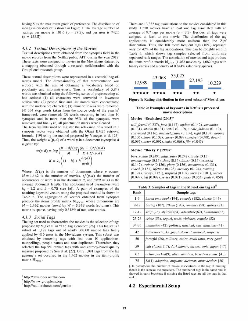
having 5 as the maximum grade of preference. The distribution of
ratings in our dataset is shown in Figure 1. The average number of
ratings per movie is 101.6 (σ = 37.5), and per user is 742.5 (σ = 188.5).
4.1.2 Textual Descriptions of the Movies
Textual descriptions were obtained from the synopsis field in the
movie records from the Netflix public API4 during the year 2012.
These texts were assigned to movies in the MovieLens dataset by
a mapping obtained through a research collaboration with the
GroupLens5 research group.
These textual descriptions were represented in a vectorial bag-of-
words model. The dimensionality of that representation was
reduced with the aim of obtaining a vocabulary based on
popularity and informativeness. Thus, a vocabulary of 5,848
words was obtained using the following series of preprocessing ad
hoc actions: (1) all characters were converted to lowercase
equivalents; (2) people first and last names were concatenated
with the underscore character; (3) numeric tokens were removed;
(4) 334 stop words taken from the source code of the gensim6
framework were removed; (5) words occurring in less than 10
synopses and in more than the 95% of the synopses, were
removed; and finally (6) all punctuation marks were cleaned.
The term weights used to register the relevance of a word in a
synopsis vector were obtained with the Okapi BM25 retrieval
formula [19] using the method proposed by Vanegas et al. [25].
Thus, the weight `(a, b) of a word a in a document (synopsis) b
is given by: `(a, b) = cde f� − bg(a)� h (i� + 1)Ug(a, b)j + Ug(a, b)
j = i� k(1 − l) + l bc(b)mnbc o
Where, bg(a) is the number of documents where a occurs, � = 1,462 is the number of movies, Ug(a, b) the number of
occurrences of word a in the document b, and mnbc = 33 is the
average document length. The additional used parameters were i� = 1.2 and l = 0.75 (see [e]). A pair of examples of the
resulting keyword vectors using the proposed method is shown in
Table 2. The aggregation of vectors obtained from synopses
produce the items profile matrix ;0×Q, whose dimensions are � = 1,462 movies (rows) by s = 5,848 words (columns). This
matrix is sparse, having only 0.518% of non-zero entries.
4.1.3 Social Tags
The tag set used to characterize the movies is the selection of tags
proposed by Vig et al. in “The Tag Genome” [26]. This tag set is a
subset of 1,128 tags out of nearly 30,000 unique tags freely
applied by 416 users in the MovieLens system. This subset was
obtained by removing tags with less than 10 applications,
misspellings, people names and near duplicates. Thereafter, they
selected the top 5% ranked tags with and entropy-based quality
measure proposed by Sen et al. [22]. Only 1,081 tags from the tag
genome’s set occurred in the 1,462 movies in the item-profile
matrix ;0�.
4 http://developer.netflix.com 5 http://www.grouplens.org 6 http://radimrehurek.com/gensim
There are 13,332 tag associations to the movies considered in this
study. 1,370 movies have at least one tag associated with an
average of 9.7 tags per movie (σ = 8.5). Besides, all tags were
assigned at least to one movie. The distribution of the tag
applications is considerably more uniform than the Zipf
distribution. Thus, the 108 more frequent tags (10%) represent
only the 42% of the tag associations. This can be roughly seen in
Table 3, which shows tag samples selected from uniformly
separated rank ranges. The association of movies and tags produce
the items profile matrix ;0� (1,462 movies by 1,082 tags) with
binary entries and a density of 0.844% (also very sparse).
Figure 1: Rating distribution in the used subset of MovieLens
Table 2: Examples of keywords in Netflix’s processed
movie descriptions
Movie: “Bewitched (2005)”
will_ferrell (0.237), jack (0.147), update (0.142), samantha
(0.131), sitcom (0.131), witch (0.119), nicole_kidman (0.119),
convinced (0.116), michael_caine (0.114), right (0.107), hoping
(0.105), know (0.103), career (0.099), perfect (0.098), doesnt
(0.097), actor (0.092), make (0.068), film (0.045)
Movie: “Rocky V (1990)”
burt_young (0.249), talia_shire (0.242), broke (0.15),
upandcoming (0.15), shots (0.15), boxer (0.15), crooked
(0.142), trainer (0.136), glory (0.136), accountant (0.131),
ended (0.131), lifetime (0.128), memory (0.124), training
(0.124), rocky (0.121), inspired (0.107), taking (0.101), career
(0.099), left (0.092), series (0.071), takes (0.063), finds (0.058)
Table 3: Samples of tags in the MovieLens tag set§
Rank Sample tags
1-3 based on a book (194), comedy (182), classic (143)
9-12 boring (107), 70mm (193), romance (98), quirky (91)
17-19 sci fi (78), stylized (64), adventure(62), humorous(62)
25-26 crime (53), sequel, tense, violence, remake (52)
34-35 animation (42), politics, satirical, war, hilarious (41)
42 bittersweet (34), gay, historical, musical, suspense
50 forceful (26), military, satire, small town, very good
59 cult classic (17), dark humor, earnest, epic, japan {17}
67 action packed(9), alien, aviation, based on comic {41}
75 3d(1), adoption, airplane, alcatraz, arms dealer: {80}
§ In parenthesis the number of movie associations to the tag; if missing,
then it is the same as the precedent. The number of tags in the same rank is
showed in curly brackets; if missing the listed tags are all the tags in that
rank.
4.2 Experimental Setup
12,98943,068 55,025
27,19310,229
����� ���� ��� �� �
13
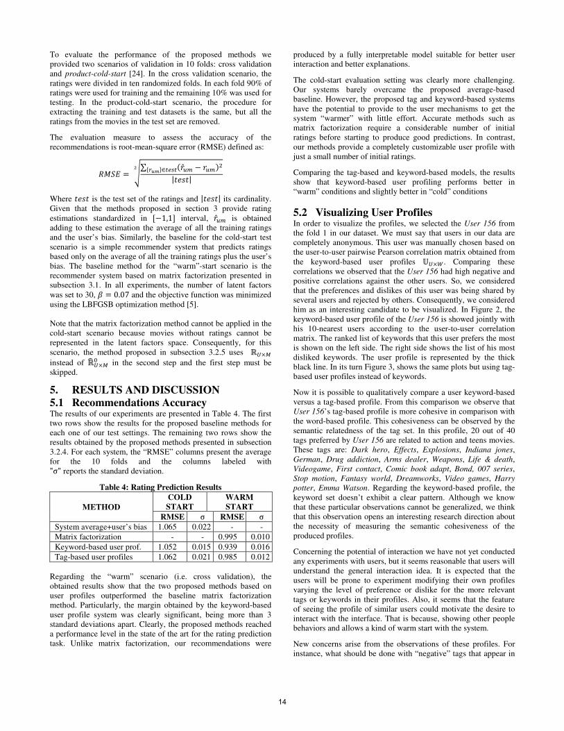
To evaluate the performance of the proposed methods we
provided two scenarios of validation in 10 folds: cross validation
and product-cold-start [24]. In the cross validation scenario, the
ratings were divided in ten randomized folds. In each fold 90% of
ratings were used for training and the remaining 10% was used for
testing. In the product-cold-start scenario, the procedure for
extracting the training and test datasets is the same, but all the
ratings from the movies in the test set are removed.
The evaluation measure to assess the accuracy of the
recommendations is root-mean-square error (RMSE) defined as:
t�uv = w∑ (��� − ���)�K1/2N∈IxyI|U zU|{
Where U zU is the test set of the ratings and |U zU| its cardinality.
Given that the methods proposed in section 3 provide rating
estimations standardized in [−1,1] interval, ��� is obtained
adding to these estimation the average of all the training ratings
and the user’s bias. Similarly, the baseline for the cold-start test
scenario is a simple recommender system that predicts ratings
based only on the average of all the training ratings plus the user’s
bias. The baseline method for the “warm”-start scenario is the
recommender system based on matrix factorization presented in
subsection 3.1. In all experiments, the number of latent factors
was set to 30, % = 0.07 and the objective function was minimized
using the LBFGSB optimization method [5].
Note that the matrix factorization method cannot be applied in the
cold-start scenario because movies without ratings cannot be
represented in the latent factors space. Consequently, for this
scenario, the method proposed in subsection 3.2.5 uses ℝ.×0
instead of ℝ9.×07 in the second step and the first step must be
skipped.
5. RESULTS AND DISCUSSION
5.1 Recommendations Accuracy
The results of our experiments are presented in Table 4. The first
two rows show the results for the proposed baseline methods for
each one of our test settings. The remaining two rows show the
results obtained by the proposed methods presented in subsection
3.2.4. For each system, the “RMSE” columns present the average
for the 10 folds and the columns labeled with "σ" reports the standard deviation.
Table 4: Rating Prediction Results
METHOD
COLD
START
WARM
START
RMSE σ RMSE σ
System average+user’s bias 1.065 0.022 - -
Matrix factorization - - 0.995 0.010
Keyword-based user prof. 1.052 0.015 0.939 0.016
Tag-based user profiles 1.062 0.021 0.985 0.012
Regarding the “warm” scenario (i.e. cross validation), the
obtained results show that the two proposed methods based on
user profiles outperformed the baseline matrix factorization
method. Particularly, the margin obtained by the keyword-based
user profile system was clearly significant, being more than 3
standard deviations apart. Clearly, the proposed methods reached
a performance level in the state of the art for the rating prediction
task. Unlike matrix factorization, our recommendations were
produced by a fully interpretable model suitable for better user
interaction and better explanations.
The cold-start evaluation setting was clearly more challenging.
Our systems barely overcame the proposed average-based
baseline. However, the proposed tag and keyword-based systems
have the potential to provide to the user mechanisms to get the
system “warmer” with little effort. Accurate methods such as
matrix factorization require a considerable number of initial
ratings before starting to produce good predictions. In contrast,
our methods provide a completely customizable user profile with
just a small number of initial ratings.
Comparing the tag-based and keyword-based models, the results
show that keyword-based user profiling performs better in
“warm” conditions and slightly better in “cold” conditions
5.2 Visualizing User Profiles
In order to visualize the profiles, we selected the User 156 from
the fold 1 in our dataset. We must say that users in our data are
completely anonymous. This user was manually chosen based on
the user-to-user pairwise Pearson correlation matrix obtained from
the keyword-based user profiles :.×Q. Comparing these
correlations we observed that the User 156 had high negative and
positive correlations against the other users. So, we considered
that the preferences and dislikes of this user was being shared by
several users and rejected by others. Consequently, we considered
him as an interesting candidate to be visualized. In Figure 2, the
keyword-based user profile of the User 156 is showed jointly with
his 10-nearest users according to the user-to-user correlation
matrix. The ranked list of keywords that this user prefers the most
is shown on the left side. The right side shows the list of his most
disliked keywords. The user profile is represented by the thick
black line. In its turn Figure 3, shows the same plots but using tag-
based user profiles instead of keywords.
Now it is possible to qualitatively compare a user keyword-based
versus a tag-based profile. From this comparison we observe that
User 156’s tag-based profile is more cohesive in comparison with
the word-based profile. This cohesiveness can be observed by the
semantic relatedness of the tag set. In this profile, 20 out of 40
tags preferred by User 156 are related to action and teens movies.
These tags are: Dark hero, Effects, Explosions, Indiana jones,
German, Drug addiction, Arms dealer, Weapons, Life & death,
Videogame, First contact, Comic book adapt, Bond, 007 series,
Stop motion, Fantasy world, Dreamworks, Video games, Harry
potter, Emma Watson. Regarding the keyword-based profile, the
keyword set doesn’t exhibit a clear pattern. Although we know
that these particular observations cannot be generalized, we think
that this observation opens an interesting research direction about
the necessity of measuring the semantic cohesiveness of the
produced profiles.
Concerning the potential of interaction we have not yet conducted
any experiments with users, but it seems reasonable that users will
understand the general interaction idea. It is expected that the
users will be prone to experiment modifying their own profiles
varying the level of preference or dislike for the more relevant
tags or keywords in their profiles. Also, it seems that the feature
of seeing the profile of similar users could motivate the desire to
interact with the interface. That is because, showing other people
behaviors and allows a kind of warm start with the system. New concerns arise from the observations of these profiles. For
instance, what should be done with “negative” tags that appear in
14

the list of preferred tags of users? This situation is illustrated by
the tag “boring!” in the User 156’s “likes” list.
Probably, this tag can be reasonable and predictive for some users,
so, maybe it shouldn’t be removed from the tag set. But trenchant
criticisms of user tastes should be prevented. A possible
alternative to this problem would be the use of a linear regression
algorithm, similar to the one used in a previous work [3], that
could estimate a weight for each tag for knowing if the tag is
intrinsically positive or negative. Thus, if a tag has a negative
connotation we could filter it from the list of “liked” tags.
Figure 2: Keyword-based profile for User 156
6. CONCLUSIONS We proposed a generic method to extract user profiles, in
interpretable spaces, in which it is possibly to directly characterize
items from the collection. The proposed user-profiling methods
were indexed in two different spaces: keywords and tags. Besides
the proposed models are suitable for user interaction in the user
profile component.
The proposed user-profiling methods were evaluated in a subset
of the MovieLens dataset and compared against strong baselines.
It was concluded that in “warm” scenarios both methods produce
recommendations with the same accuracy than those produced by
matrix factorization methods. In a cold-start scenario, both
methods performed slightly better than a recommender system
based on average ratings.
In the warm-start scenario, when the keyword-based profiling and
the tag-based profiling methods are compared, it was observed
that keyword-based method was considerably more accurate than
the matrix factorization method. The RMSE decremented by a
5.63% (more than 3 times σ), while the difference in the error
with the tab-based method was only 1.00%. Consequently, it is
possible to say that the proposed keyword-based method is able to
improve the matrix factorization approach.
Figure 3: Tag-based profile for User 156
Regarding the proposed visualization of the keyword-based and
the tag-based user profiles, we could observe that cohesion of the
profile is an important measure to have into account when two
profiles methods are compared. Non-cohesive profiles might be
misunderstood by users leading them to avoid the interaction with
those profiles. An interesting research question could be how to
discriminate cohesive profiles, from non-cohesive profiles.
The proposed approach also contributed to a better classification
of the content-based recommendation techniques, separating the
user-profiling task from the item-profiling task, suggesting a
uniform framework to share and compare the contributions made
on each one of the tasks.
7. ACKNOWLEDGMENTS
15

Our especial thanks to Prof. John Riedl and Daniel Kluver from
GroupLens, the University of Minnesota; Prof. Shilad Sen of the
Macalester College; and Prof. Fabio Gonzalez of the Universidad
Nacional de Colombia. The work was partially funded by the
Colombian Department for Science, Technology and Innovation
(Colciencias) via the grant 1101-521-28465 from “El Patrimonio
Autónomo Fondo Nacional de Financiamiento para la Ciencia, la
Tecnología y la Innovación, Francisco José de Caldas” and by the
Universidad Nacional de Colombia via the grant DIB QUIPU:
201010016956. The third author recognizes the support from
Mexican Government (SNI, COFAA-IPN, SIP 20131702,
CONACYT 50206-H) and CONACYT–DST India (grant 122030
“Answer Validation through Textual Entailment”).
7. REFERENCES [1] Adomavicius, G., Manouselis, N. and Kwon, Y. 2011.
Multi-Criteria Recommender Systems. Recommender
Systems Handbook. 769–803.
[2] Man Au Yeung, C., Gibbins, N. and Shadbolt, N. 2008. A
Study of User Profile Generation from Folksonomies.
SWKM (2008).
[3] Becerra, C., Gonzalez, F. and Gelbukh, A. 2011.
Visualizable and Explicable Recommendations Obtained
from Price Estimation Functions. Proceedings of the
Human Decision Making in Recommender Systems (2011),
27–34.
[4] Bell R.M., Koren Y. and C, V. 2007. The BellKor solution
to the Net Flix Prize. Technical report, AT&T Labs
Research. (2007).
[5] Byrd, R.H., Lu, P., Nocedal, J. and Zhu, C. 1995. A limited
memory algorithm for bound constrained optimization.
SIAM J. Sci. Comput. 16, 5 (Sep. 1995), 1190–1208.
[6] Diederich, J. and Iofciu, T. 2006. Finding Communities of
Practice from User Profiles Based On Folksonomies.
Proceedings of the 1st International Workshop on Building
Technology Enhanced Learning solutions for Communities
of Practice (2006).
[7] Fellbaum, C. ed. 1998. WordNet An Electronic Lexical
Database. The MIT Press.
[8] De Gemmis, M., Lops, P., Semeraro, G. and Basile, P.
2008. Integrating tags in a semantic content-based
recommender. Proceedings of the 2008 ACM conference
on Recommender systems (New York, NY, USA, 2008),
163–170.
[9] Guan, Z., Wang, C., Bu, J., Chen, C., Yang, K., Cai, D. and
He, X. 2010. Document recommendation in social tagging
services. Proceedings of the 19th international conference
on World wide web (New York, NY, USA, 2010), 391–
400.
[10] Hassan-Montero, Y. and Herrero-Solana, V. 2006.
Improving tag-clouds as visual information retrieval
interfaces. International Conference on Multidisciplinary
Information Sciences and Technologies (2006), 25–28.
[11] Herlocker, J.L., Konstan, J.A. and Riedl, J. 2000.
Explaining collaborative filtering recommendations.
(2000), 241–250.
[12] Hwang, C.L. and Yoon, K.M. 1981. Multiple Attribute
Decision Making. Methods and Applications. Springer-
Verlag, NY. (1981).
[13] Hwang, C.L. and Yoon, K.M. 1981. Multiple Attribute
Decision Making. Methods and Applications. Springer-
Verlag, NY. (1981).
[14] Jones, K.S. 1972. A statistical interpretation of term
specificity and its application in retrieval. Journal of
Documentation. 28, (1972), 11–21.
[15] Koren, Y., Bell, R. and Volinsky, C. 2009. Matrix
Factorization Techniques for Recommender Systems.
Computer. 42, 8 (Aug. 2009), 30–37.
[16] Lops, P., Gemmis, M. and Semeraro, G. 2011. Content-
based Recommender Systems: State of the Art and Trends.
Recommender Systems Handbook. F. Ricci, L. Rokach, B.
Shapira, and P.B. Kantor, eds. Springer US. 73–105.
[17] Lops, P., Gemmis, M., Semeraro, G., Musto, C., Narducci,
F. and Bux, M. 2009. A Semantic Content-Based
Recommender System Integrating Folksonomies for
Personalized Access. Web Personalization in Intelligent
Environments. G. Castellano, L. Jain, and A. Fanelli, eds.
Springer Berlin Heidelberg. 27–47.
[18] Penrose, R. and Todd, J.A. On best approximate solutions
of linear matrix equations. Mathematical Proceedings of
the Cambridge Philosophical Society. null, 01, 17–19.
[19] Robertson, S. 2005. How Okapi Came to TREC. TREC:
Experiment in Information Retrieval. MIT Press. 287–300.
[20] Salton, G., Wong, A.K.C. and Yang, C.-S. 1975. A vector
space model for automatic indexing. Commun. ACM.
18(11), (1975), 613–620.
[21] Schein, A., Pennock, D. and Ungar 2002. Methods and
metrics for cold-start recommendations. SIGIR (2002).
[22] Sen, S., Harper, F.M., LaPitz, A. and Riedl, J. 2007. The
quest for quality tags. Proceedings of the 2007
International ACM Conference on Supporting Group Work
(2007), 361–370.
[23] Sen, S., Vig, J. and Riedl, J. 2009. Learning to recognize
valuable tags. Proceedings of the 13th International
Conference on Intelligent User Interfaces (Sanibel Island,
Florida, USA, 2009), 87–96.
[24] Smola, A.J. and Schölkopf, B. 1998. A Tutorial on Support
Vector Regression,. Royal Holloway College, London,
U.K., NeuroCOLT Tech. Rep..TR 1998-030, 1998. (1998).
[25] Vanegas, J.A., Caicedo, J.C., Camargo, J.E. and Ramos-
Pollán, R. 2012. Bioingenium at ImageCLEF 2012:
Textual and Visual Indexing for Medical Images. CLEF
(Online Working Notes/Labs/Workshop) (Rome, Italy,
2012).
[26] Vig, Jesse, Sen, S. and Riedl, J. The Tag Genome:
Encoding Community Knowledge to Support Novel
Interaction. ACM Transactions on Interactive Inteligent
Systems. 2, 3.
[27] Yeh, C.H. 2002. A problem based selection of multi-
attribute decision-making methods. International
Transactions in Operational Research. 9, 2 (Mar. 2002),
169–181.
[28] Yoon, K. and Hwang, C. 1995. Multiple Attribute Decision
Making. An introduction. Sage university papers series,
no. 07-104. Thousand Oaks, CA: Sage Publications.
(1995).
[29] Zhang, Z.-K., Zhou, T. and Zhang, Y.-C. 2011. Tag-Aware
Recommender Systems: A State-of-the-Art Survey.
Journal of Computer Science and Technology. 26, 5 (Sep.
2011), 767–777.
[30] Zopounidis, C. and Doumpos, M. 2002. Multicriteria
classification and sorting methods: A literature review.
European Journal of Operational Research. 138, 2 (Apr.
2002), 229–246.
16
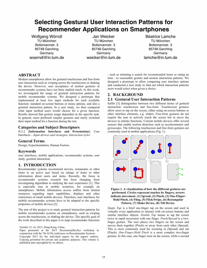
Selecting Gestural User Interaction Patterns for Recommender Applications on Smartphones
Wolfgang Wörndl TU München
Boltzmannstr. 3 85748 Garching
Germany [email protected]
Jan Weicker TU München
Boltzmannstr. 3 85748 Garching
Germany [email protected]
Béatrice Lamche TU München
Boltzmannstr. 3 85748 Garching
Germany [email protected]
ABSTRACT Modern smartphones allow for gestural touchscreen and free-form user interaction such as swiping across the touchscreen or shaking the device. However, user acceptance of motion gestures in recommender systems have not been studied much. In this work, we investigated the usage of gestural interaction patterns for mobile recommender systems. We designed a prototype that implemented at least two input methods for each available function: standard on-screen buttons or menu options, and also a gestural interaction pattern. In a user study, we then compared what input method users would choose for a given function. Results showed that gesture usage depended on the specific task. In general, users preferred simpler gestures and rarely switched their input method for a function during the test.
Categories and Subject Descriptors H.5.2 [Information Interfaces and Presentation]: User Interfaces – Input devices and strategies, Interaction styles
General Terms Design, Experimentation, Human Factors.
Keywords user interfaces, mobile applications, recommender systems, user study, gestural interaction.
1. INTRODUCTION Recommender systems recommend movies, restaurants or other items to an active user based on ratings of items or other information about users and items. Recently, the focus in recommender systems research has been changing from investigating algorithms to studying the user experience [1]. This is especially true in mobile scenarios, for example on smartphones. Mobile information access suffers from limited resources regarding input capabilities, displays and other restrictions of small mobile devices. Therefore, user interfaces for mobile recommender systems have to be adapted to the specific properties of mobile devices [2].
The aim of this project is to study gestural interaction patterns for mobile recommender systems on smartphones, such as swiping across the touchscreen, or shaking the device. The specific goal of the work described in this paper is to map recommender functions
- such as initiating a search for recommended items or rating an item - to reasonable gesture and motion interaction patterns. We designed a prototype to allow comparing user interface options and conducted a user study to find out which interaction patterns users would select when given a choice.
2. BACKGROUND 2.1 Gestural User Interaction Patterns Saffer [3] distinguishes between two different forms of gestural interaction: touchscreen and free-form. Touchscreen gestures allow users to tap on the screen, either using on-screen buttons or other interface elements, e.g. sliders. Free-form gestures do not require the user to actively touch the screen but to move the devices to initiate functions. Current mobile devices offer several sensors that enable motion detection such as accelerometers and gyroscopes. The following touchscreen and free-form gestures are commonly used in mobile applications (Fig. 1).
Figure 1. A visualization of how the different gestures are performed. Circles represent touches by fingers, arrows
indicate movement. (1) Spread, (2) Pinch, (3) One-Finger-Hold Pinch, (4) Fling, (5) Flick/Swipe, (6) Rectangular
Pattern, (7) Shake Device, (8) Tilt Device. Single Tap is a brief one-finger tap on the screen and used in virtually every application to interact with on-screen buttons and similar interface objects. Double Tap means to tap the screen twice in rapid succession with one finger. Pinch/Spread is a two-finger gesture. The user places two fingers on the screen and moves them together (Pinch) or away from each other (Spread). This is most commonly used for zooming in (Spread) and out (Pinch). One-Finger-Hold Pinch is a more complex two-finger gesture. In this case, one finger rests on the screen, while a second
October 12–16, 2013, Hong Kong, China. Paper presented at the 2013 Decisions@RecSys workshop in conjunction with the 7th ACM conference on Recommender Systems. Copyright 2013 for the individual papers by the papers' authors. Copying permitted for private and academic purposes. This volume is published and copyrighted by its editors.
17

finger moves on the screen to adjust a slider or other numerical value, for example.
Slide means to move a single finger over the screen in a continuous motion. Slide is generally used for dragging objects like sliders and slowly scrolling through views exceeding the screen’s dimensions. Fling is a quick, long movement of one finger in one direction and can also be used for quickly scrolling through list views. Flick (or Swipe) is a shorter gesture similar to the longer Fling and commonly used as Swipe-To-Delete in file systems: a Flick gesture performed on an item generally deletes this item from a list. Another usage is moving to the next screen, resembling turning pages in a book. Shake Device and Tilt Device (along x, y or z axis) are free-form motion gestures with no screen interaction required.
Technically, any touch pattern can be drawn on the screen using one or more fingers, e.g. a rectangular pattern. However, finding the balance between gesture detection precise enough to distinguish different patterns, and vague enough to allow for user errors when drawing the patterns is difficult. In addition, explaining complex patterns to the user is challenging and therefore, complex patterns are rarely used in mobile applications.
2.2 Related Work Previous research on the usage of gestures in mobile scenarios focused on the user acceptance of motion gestures in general and hardly applied these techniques for the interaction with recommender systems. In own previous work, we designed a minimalistic user interface for a map-based recommender based on gestural interaction, but for the larger screens of tablets [4]. Cho et al. propose a photo browsing system for mobile devices. They compared three types of interaction: a tilt-based interaction technique, an iPod wheel and a button-based browser to browse and search photos efficiently. The results show that the tilting technique is comparable to the controllability of buttons, more interesting than the other techniques and performed better than the iPod wheel [5]. Negulescu et al. examined the cognitive demands of motion gestures, taps and surface gestures. They show that these three techniques do not differ in reaction time. Moreover they found out that motion gestures result in much less time spent looking at the smartphone during walking than does tapping on the screen. Therefore motion gestures are advantageous in certain scenarios [6]. Rico and Brewster applied a different focus on motion gestures for mobile devices. They found out that location and audience have a significant influence on a user’s willingness to interact with a mobile device by using motion gestures [7].
3. DESIGNING THE TEST APPLICATION 3.1 Overview We implemented the prototype application for Android 2.2 (Froyo) and tested it on a Google Nexus One smartphone with Android. The goal of the test application was to provide different input methods for functions typically found in recommender systems to test which interaction patterns the user would chose in the successive study. The selection of functions in our application is not really specific to mobile recommenders and considers recommenders in a wider sense, i.e. taking also "search" applications into account. The scenario for the prototype is a movie search and recommendation application that resembles the Internet Movie Database (IMDb) mobile application (see http://www.imdb.com/apps).
We provided at least two different input methods for each application function, either
• on-screen buttons, • menu options (the user has to select a specific "menu"
option1 to show additional buttons), or • gestural interface options (cf. Section 2.1).
The next subsection describes considerations for mapping gestures to application-specific functions.
3.2 Considerations for Mapping Gestures to Application-Specific Functions Single Tap is commonly used for interaction with on-screen interface objects and should not be used for other application-specific purposes. The same applies to Slide and Fling for scrolling screens or dragging objects. Contrariwise, Double Tap is not bound to any standard features and thus application-specific features can be mapped to it. As Pinch/Spread is generally used for zooming, mapping it to other application features may be confusing as well. However, the One-Finger-Hold Pinch (OFHP) variation of this gesture is applied in our application.
Since no screen interaction is necessary for the free-form gesture Shake Device, this gesture may be used independently from any interface restrictions, for example for application-wide functions. An application-wide function can be called at any time, regardless of the current screen of the application, e.g. the "home" button on most mobile systems. Functions depending on viewing items on-screen may not be viable for use with Shake Device, since shaking the screen makes focusing on displayed objects on the screen harder. The nature of the other motion gesture, Tilt Device, suggests either a use for simple actions like a binary +/- rating (making use of the left-right or front-back movements of Tilt Device), or for any navigation function along two or three axes. Tilt Device is not applied in our test application, because the application does not use binary ratings.
3.3 Test Application User Interface In the test application, the user can use a search interface to select among movie genres and find items. The search interface can be reached from the start screen, main menu or through the options menu. After searching, a list of corresponding items is shown (Fig. 2, left). Users can scroll up and down the list, remove items from the list or select an item to display more details by using Single Tap. The item details screen (Fig. 2, right) shows information for the selected movie and allows for bookmarking and rating the item. In addition, an options menu is available on every screen to return to the search screen or main menu of the application (Fig. 2, right). The following functions are available and implemented by at least two input options each:
• Bookmark: The user can bookmark an item by using on-screen or options menu buttons (Fig. 2, right), or by using the Double Tap gesture in the item details screen
• Find Random Item: Accessible application-wide through the options menu or by using the Shake Device gesture
• Save Search Parameters: This function is available in the search screen via an on-screen button or by a Double Tap in this screen
• Find Similar: The item details screen shows three movies similar to the selected one ("similar to this
1 On most systems, a dedicated software or hardware button opens
up the options menu
18

movie" part in Fig. 2, right). The user has the option to find more similar items by using an on-screen button or the Flick gesture
• Exclude Item: Available in the list view as an on-screen button (Fig. 2, left) or via the Flick gesture
• Rate Item: Users can rate items in the item details screen by selecting the "Rate" on-screen button (Fig. 2, right). Then, a rating scale of 1 to 10 stars appears. The user can set his or her desired rating by either using the rating scale as an on-screen button or applying the One-Finger-Hold Pinch (cf. Section 2.1) gesture.
Figure 2. List of recommendations (left). Item details with options menu (right).
4. USER STUDY
4.1 Study Setup and Methodology We have conducted a user study to find out what input method for a given function is preferred by the test users. The evaluation was performed with each of the participants individually. To start, each user was given an explanation of the application and was then allowed to practice navigating the different functions and input methods for about ten minutes. The participants then had to perform a set of 18 instructions in the application in a certain order. The list mentioned the required tasks only; the input method to perform them was not specified. By doing so, we tested which input method the test persons found more intuitive to use for a certain task. The beginning of the sequence of instructions read as follows: (1) Find Random Item, (2) Find Similar Item, (3) Rate Item, (4) Open Main Menu, (5) Open My Recommendations, (6) Exclude Item from Recommendations, and so on. Some of the requested functions appeared several times in the list, for example Find Random Item was requested three times. This was used to test whether participants would change their preferred input method for a particular function during the experiment.
We recorded every user action in a log file. After a test user completed the scenario, he or she had to fill out a survey concerning his or her opinions about the input methods for the requested instructions and about the handling of the gestures in particular.
4.2 Log File Analysis 16 persons with mixed backgrounds participated in the study. Other than a few users skipping a few tasks from the instruction list, all subjects completed the given scenario. We first analyzed the log file to understand which input options the users chose to complete a given task.
Out of a total of 44 recorded usages, the Find Random function was initiated 26 times using the Shake Device gesture, and 18 times using the options menu button (see Fig. 2, right). This represents a 59.1% usage rate for the implemented gesture. Interestingly, only one out of the 16 users elected to use both available input methods; every other user exclusively used either the gesture or the button for the three instances of Find Random in our instruction list. The Bookmark Item function is represented three times in the scenario. The users chose to use the Double Tap gesture 27 out of 46 times (58.7%). However, at one instance in the scenario, the activity in focus is the item list, which only implements bookmarking via double tapping. In this case, 11 of 16 users (68.8%) chose the Double Tap gesture, while the rest of the users elected to take additional time to first open an item’s details page and bookmark there. While the users were on an item’s details page, they called only 16 of 35 (45.7%) instances of Bookmark Item using the Double Tap gesture. All differences to 100% in this paragraph are due to the uses of the on-screen bookmark button – the options menu button was never used.
The use of the Save Search Parameters function was requested only once in the scenario and can be called using Double Tap or an on-screen button. This is the function with the clearest favorite among the input methods: 15 out of 16 users (93.8%) chose the on-screen button.
The scenario contained two instances of the Exclude Recommended Item function, operable via Flick gesture or an on-screen button. 18 of 32 (56.3%) calls were made using gestural interaction. A relatively high number of users used both input methods for this task: 4 out of 16 participants (25%). This is even though the two instances of the Exclude Recommended Item task occurred directly after each other in our task list. Rate Item and Find Similar Item each occur two times in the scenario. For both, a clear preference towards the standard input method of an on-screen button can be seen: for Rate Item, only 10 of 32 instances (31.3%) were operated with the One-Finger-Hold Pinch gesture. Even more one-sided, the Find Similar Item function was only initiated using Flick in 3 of 32 cases (9.4%). The remaining percentages represent instances of functions called via on-screen button.
4.3 Survey Results In the first part of the survey we asked the participants how intuitive they find the input methods for the six functions on a scale from 1 to 5. Figure 3 illustrates the results with a higher number meaning "more intuitive". In general, the results correspond to the log file very well: input methods that were actually preferred and used by the participants received higher grades for intuitivity. For example, the participants find the on-screen buttons for Save Search and Find Similar very intuitive. On the other hand, the Shake Device for Find Random Item, Double Tap for Bookmark and Flick for Exclude Item gestures received higher grades in comparison with on-screen or option menu buttons.
19

Figure 3. Average of users' ratings how intuitive each
function’s input method was. The next question was whether inclusion of an on-screen button was worth the necessary screen space for it. Our users mostly were in favor of it: the majority of users denied this question for Exclude Item only (Fig. 4). Interestingly, this is the only on-screen button in the list view (Fig. 2).
Figure 4. Screen space usage for on-screen buttons
The goal of the next part of the survey was to determine the user’s favorite input method for each function. The distribution of choices for each function is shown in Fig. 5 and is comparable to the grades for intuitivity: interaction patterns that users perceived as intuitive were chosen as favorite input method.
Figure 5. Selecting only one input option for each function
We also asked the test users about their prior experience with touchscreen devices and analyzed whether it would relate to differences in the results. The most significant difference was that 62.5% of the users with more prior touchscreen experience rated the Shake Device gesture as intuitive, while only 12.5% did so among the users with less experience. We noted a similar difference regarding the Flick gesture.
Concerning the ease of handling of the four gestures, the participants considered all gestures, except One-Finger-Hold Pinch (OFHP), as easy to handle in general. One of the problems with OFHP was that lifting a finger while adjusting the desired rating for item ends the rating process. In addition, the calibration for the rating scale of one to ten stars was difficult. So this gesture might be more suitable for simpler tasks with fewer options.
5. DISCUSSION AND CONCLUSION The results of the study presented in this work may be used to improve the design of user interfaces for mobile recommender systems and other similar applications. Our study showed that
users preferred the simpler, easier to handle gestures over the more complex ones. Complex gestures like One-Finger-Hold Pinch must be carefully calibrated for ease of handling. Omitting on-screen buttons is only an option in activities where content space is rare, in our case the overview list of items. For the item detail screen, simply touching a button was the favorite input method most of the times. The options menu was not very popular in any of the used cases. This is likely due to the fact that opening the options menu is an extra effort that users do not tend to make when other input methods are available.
While Double Tap for bookmarking items was received very well, the Double Tap gesture for Save Search Parameters was not very popular and received low grades for intuitivity. This may be due to the layout of the corresponding screens because users might have the fear of accidently tapping on other interface elements. In essence, the use of gestural interaction patterns seems to depend on the actual screen and function detail. Interestingly, users did not change their preferred input mode much during the test: they mostly used the same method for the same task throughout the scenario. Users with more experience with touchscreen devices were more open towards gestures than users with less experience.
Future work includes studying in more detail how more complex gestures can be introduced in mobile recommender systems to improve user interaction. Moreover, a long-term study would be interesting because user acceptance might change if smartphone users get more and more used to complex motion gestures.
6. REFERENCES [1] Konstan, J.A., and Riedl, J. 2012. Recommender systems:
from algorithms to user experience. User Model. User-Adapt. Interact. 22, 1-2 (April 2012), 101-123. DOI= http://dx.doi.org/10.1007/s11257-011-9112-x.
[2] Ricci, F. 2011. Mobile recommender systems. J. of IT & Tourism. 12, 3 (April 2010), 205-231. DOI= http://dx.doi.org/10.3727/109830511X12978702284390.
[3] Saffer, D. 2008. Designing Gestural Interfaces. O'Reilly, Sebastopol.
[4] Schulze, F., Woerndl, W., and Ludwig, M. 2012. A gesture-based interface for map-based exploratory search on tablets. In Proc. Mobility and Web Behavior Workshop, MobileHCI '12 Conference (San Francisco, CA, September 21 – 24, 2012).
[5] Cho, S.J., Murray-Smith, R. and Kim, Y.B. 2007. Multi-context photo browsing on mobile devices based on tilt dynamics. In Proc. of the 9th International Conference on Human Computer Interaction with Mobile Devices and Services (Singapore, September 09 – 12, 2007). MobileHCI '07. ACM, New York, NY, 190-197. DOI= http://doi.acm.org/10.1145/1377999.1378006.
[6] Negulescu, M., Ruiz, J., Li, Y., and Lank, E. 2012. Tap, swipe, or move: attentional demands for distracted smartphone input. In Proc. of the Int. Working Conference on Advanced Visual Interfaces (Capri Island, Italy, May 21 – 25, 2012). AVI '12. ACM, New York, NY, 173-180. DOI= http://doi.acm.org/10.1145/2254556.2254589.
[7] Rico, J., and Brewster, S. 2010. Usable gestures for mobile interfaces: evaluating social acceptability. In Proc. of the SIGCHI Conference on Human Factors in Computing Systems (Atlanta, GA, April 10 – 15, 2010). CHI '10. ACM, New York, NY, 887-896. DOI= http://doi.acm.org/10.1145/1753326.1753458.
20

The Role of Emotions in Context-aware Recommendation
Yong Zheng, Robin Burke, Bamshad MobasherCenter for Web Intelligence
School of Computing, DePaul UniversityChicago, Illinois, USA
{yzheng8, rburke, mobasher}@cs.depaul.edu
ABSTRACTContext-aware recommender systems try to adapt to users’ pref-erences across different contexts and have been proven to providebetter predictive performance in a number of domains. Emotion isone of the most popular contextual variables, but few researcher-s have explored how emotions take effect in recommendations –especially the usage of the emotional variables other than the ef-fectiveness alone. In this paper, we explore the role of emotions incontext-aware recommendation algorithms. More specifically, weevaluate two types of popular context-aware recommendation algo-rithms – context-aware splitting approaches and differential contextmodeling. We examine predictive performance, and also explorethe usage of emotions to discover how emotional features interactwith those context-aware recommendation algorithms in the rec-ommendation process.
Categories and Subject DescriptorsH.3.3 [Information Search and Retrieval]: Information filtering
General TermsAlgorithm, Experiment, Performance
KeywordsRecommendation, Context, Context-aware recommendation, Emo-tion, Affective recommender system
1. INTRODUCTIONAdvances in affective computing have enabled recommender sys-tems to take advantage of emotions and personality, leading to thedevelopment of affective recommender systems (ARS) [18]. Atthe same time, the emerging technique of context-aware recom-mender systems (CARS) takes contexts into consideration, convert-ing a two-dimensional matrix of ratings organized by user and item:Users× Items→ Ratings, into a multidimensional rating space [1].CARS have been demonstrated to be effective in a variety of appli-cations and domains [4, 15, 10, 24, 13]. Emotional variables areoften included as contexts in CARS, which enables the further de-velopment of both ARS and CARS. Typical emotional contexts in
RecSys’13, October 12–16, 2013, Hong Kong, China.Paper presented at the 2013 Decisions@RecSys workshop in conjunc-tion with the 7th ACM conference on Recommender Systems. Copyrightc©2013 for the individual papers by the papers’ authors. Copying permitted
for private and academic purposes. This volume is published and copyright-ed by its editors.
recommender system domain are the ones relevant to users’ subjectmoods or feelings, for example, user mood when listening to musictracks (e.g. happy, sad, aggressive, relaxed, etc) [19, 9], or users’emotions after seeing a movie (e.g. user may feel sad after seeinga tragic movie) [13].
Emotional context was first exploited by Gonzalez et al [8] forthe recommender system domain. This work was followed by oth-ers [9, 18, 13, 17] considering emotions as contexts in CARS re-search. While the effectiveness of emotions as contextual variablesis therefore well-established, there is little research that has exam-ined specifically the role that these emotional variables play. Wedefine "the role of emotions" as the concerns from two aspects –whether emotions are useful or effective to improve recommenda-tion performance? And, the usage of emotions in the recommen-dation process – how emotions are used in the recommendationalgorithms, e.g. which emotional variables are selected? whichalgorithm components are they applied to? and so forth. Current-ly, most research are focused on demonstrating the effectiveness ofemotional variables, and few research further explore the usage ofthe emotions in the recommendation process.
In this paper, we explore the role of emotions by two classesof popular context-aware recommendation algorithms – context-aware splitting and differential context modeling. Since both ofthese approaches require that the algorithm learn the importanceand utility of different contextual features, they help reveal howemotions work in each algorithm and what roles they can play inrecommendation.
The purpose of this study is therefore to address the followingresearch questions:
1. Emotional Effect: Are emotions useful contextual variablesfor context-aware recommendation?
2. Algorithm Comparison: What algorithms are best suited tomake use of emotional variables? Do they outperform thebaseline algorithms?
3. Usage of Contexts: How do emotional variables competewith other contextual variables, such as location and time?
4. Roles: How can we understand the specific roles emotionalvariables can play in those context-aware recommendationalgorithms?
2. RELATED WORKGonzalez et al [8] explored emotional context in recommender sys-tems in 2007. They pointed out that,"emotions are crucial for us-er’s decision making in recommendation process. The users alwaystransmit their decisions together with emotions." With the rapid de-velopment of context-aware recommender systems, emotion turns
21

out to be one of important and popular contexts in different kindsof domains, especially in the music and movie domain. For mu-sic recommendation, the emotional context is appealing because itcan be used to establish a bridge between music items and item-s from other different domains, and perform cross-media recom-mendations [6, 1, 9]. Movie recommendation is another domainwhere emotion turns out to be popular in recent years. In 2010,Yue et al [16] produced the overall winner in a recent challengeon context-aware movie recommendation by mining mood-specificmovie similarity with matrix factorization. More recent research[18, 13] motivates the tendency of taking emotions as contextsto assist contextual recommendations. Research has demonstrat-ed that emotions can be influential contextual variables in makingrecommendations, but few of them explore how emotions interactwith recommendation algorithm – the usage of emotional variablesin the recommendation process.
As described in [1], there are three basic approaches to devel-op context-aware recommendation algorithms: pre-filtering, post-filtering, and contextual modeling. A pre-filtering approach appliesa context-dependent criterion to the list of items, selecting thoseappropriate to a given context. Only the filtered items are con-sidered for recommendation. A post-filtering approach is similarbut applies the filter after recommendations have been computed.Contextual modeling takes contextual considerations into the rec-ommendation algorithm itself. In this paper, we explore context-aware splitting approaches (a class of pre-filtering algorithms), anddifferential context modeling (a contextual modeling approach.)
The remainder of this paper is organized as follows. In Sec-tion 3 and Section 4, we formally introduce the two types of recom-mendation algorithms we are studying, including their capability tocapture the role of emotional contexts in recommendation process.Sections 5 and 6 discuss the experimental evaluations and miningthe role of emotions through those context-aware recommendationalgorithms, followed by the conclusions and future work in Sec-tion 7.
3. CONTEXT-AWARE SPLITTINGAPPROACHES
Contextual pre-filtering is popular as it is straightforward to imple-ment, and can be applied with most recommendation techniques.Item splitting [4, 5] is considered one of the most efficient pre-filtering algorithms and it has been well developed in recent re-search. The underlying idea of item splitting is that the nature ofan item, from the user’s point of view, may change in differentcontextual conditions, hence it may be useful to consider it as t-wo different items [5]. User splitting [2, 15] is based on a similarintuition – it may be useful to consider one user as two differentusers, if he or she demonstrates significantly different preferencesacross contexts. In this section, we introduce those two approachesand also propose a new splitting approach – UI splitting, a simplecombination of item and user splitting.
To better understand and represent the splitting approaches, con-sider the following movie recommendation example:
Table 1: Movie Ratings in Contexts
User Item Rating Time Location CompanionU1 T1 3 Weekend Home FriendU1 T1 5 Weekend Cinema GirlfriendU1 T1 ? Weekday Home Family
In Table 1, there are one user U1, one item T1 and two ratings
(the first two rows) in the training data and one unknown rating thatwe are trying to predict (the third row). There are three contextualdimensions – time (weekend or weekday), location (at home or cin-ema) and companion (friend, girlfriend or family). In the followingdiscussion, we use contextual dimension to denote the contextu-al variable, e.g. "Location" in this example. The term contextualcondition refers to a specific value in a contextual dimension, e.g."home" and "cinema" are two contextual conditions for "Location".
3.1 Item SplittingItem splitting tries to find a contextual condition on which to spliteach item. The split should be performed once the algorithm iden-tifies a contextual condition in which items are rated significantlydifferently. In the movie example above, there are three contextu-al conditions in the dimension companion: friend, girlfriend andfamily. Correspondingly, there are three possible alternative con-ditions: "friend and not friend", "girlfriend and not girlfriend","family and not family". Impurity criteria [4] are used to deter-mine whether and how much items were rated differently in thesealternative conditions, for example a t-test or other statistical met-ric can be used to evaluate if the means differ significantly acrossconditions.
Item splitting iterates over all contextual conditions in each con-text dimension and evaluates the splits based on the impurity cri-teria. It finds the best split for each item in the rating matrix andthen items are split into two new ones, where contexts are elimi-nated from the original matrix – it transforms the original multi-dimensional rating matrix to a 2D matrix as a result. Assume thatthe best contextual condition to split item T1 in Table 1 is "Loca-tion = home and not home", T1 can be split into T11 (movie T1being seen at home) and T12 (movie T1 being seen not at home).Once the best split has been identified, the rating matrix can betransformed as shown by Table 2(a).
This example shows a simple split, in which a single contextualcondition is used to split the item. It is also possible to perform acomplex split using multiple conditions across multiple context di-mensions. However, as discussed in [5], there are significant costsof sparsity and potential overfitting when using multiple conditions.We use only simple splitting in this work.
Table 2: Transformed Rating Matrix
(a) by Item Splitting
User Item RatingU1 T11 3U1 T12 5U1 T11 ?
(b) by User Splitting
User Item RatingU12 T1 3U12 T1 5U11 T1 ?
(c) by UI Splitting
User Item RatingU12 T11 3U12 T12 5U11 T11 ?
3.2 User SplittingSimilarly, user splitting tries to split users instead of items. It canbe easily derived from item splitting as introduced above. Similarimpurity criteria can also be used for user splits. Assume that thebest split for user U1 in Table 1 is "Companion = family and notfamily", U1 can be split into U11 (U1 saw the movie with family)and U12 (U1 saw the movie with others). The rating matrix can
22

be transformed as shown by Table 2(b). The first two rows containthe same user U12 because U1 saw this movie with others (i.e. notfamily) rather than family as shown in the original rating matrix.
3.3 UI SplittingUI splitting is a new approach proposed in this paper – it appliesitem splitting and user splitting together. Assuming that the bestsplit for item and user splitting are the same as described above,the rating matrix based on UI splitting can be shown as Table 2(c).Here we see that both users and items were transformed, creatingnew users and new items.
Thus, given n items, m users, k contextual dimensions and d dis-tinct conditions for each dimension, the time complexity for thosethree splitting approaches is the same as O(nmkd) [5]. The pro-cess in UI splitting is simply an application of item splitting fol-lowed by user splitting on the resulting output. We keep the con-textual information in the matrix after the transformation by itemsplitting so that user splitting can be performed afterwards.
3.4 Role of Emotions in SplittingContext-aware splitting approaches have been demonstrated to im-prove predictive performance in previous research, but few of thoseresearch results report on the details of the splitting process. Morespecifically, it is useful to know which contextual dimensions andconditions are selected, and the statistics related to those selection-s. For our purposes, it is possible to explore how emotions interactwith the splitting process by the usage of contexts in the splittingprocess, which may help discover the role of emotions from thisperspective. In this paper, we try all three context-aware splittingapproaches, empirically compare their predictive performance, andalso explore the distributions of the usage of contexts (emotionalvariables included) for splitting operations.
4. DIFFERENTIAL CONTEXT MODELINGDifferential context modeling (DCM) is a general contextual rec-ommendation framework proposed in [23]. It can be applied toany recommendation algorithm. The "differential" part of the tech-nique tries to break down a recommendation algorithm into differ-ent functional components to which contextual constraints can beapplied. The contextual effect for each component is maximized,and the joint effects of all components contribute the best perfor-mance for the whole algorithm. The "modeling" part is focused onhow to model the contextual constraints. There are two approach-es: context relaxation and context weighting, where context relax-ation uses an optimal subset of contextual dimensions, and contextweighting assigns different weights to each contextual factor. Ac-cordingly, we have two approaches in DCM: differential contextrelaxation (DCR) [21, 22, 20] and differential context weighting(DCW) [24].
4.1 DCM in UBCFWe have successfully applied DCM to user-based collaborative fil-tering (UBCF), item-based collaborative filtering (IBCF) and Slope-One recommendation algorithms in our previous research [23], show-ing that DCM is an efficient approach to improve context-awareprediction accuracy. However, we did not explore much about themodeling part in our previous work; that is, how contexts are se-lected, relaxed or weighted.
Recall that we separate different functional components from therecommendation algorithm, therefore, how the algorithms relax orweigh contextual variables can tell the role of the contexts in diff-erent components. In this paper, we continue to apply DCM to
UBCF, where the four components we separate in UBCF can bedescribed as follows:
Figure 1: Algorithm Components in UBCF
Figure 1 shows the original rating prediction by the well-knownResnick’s UBCF algorithm [14], where a is a user, i is an item,and N is a neighborhood of K users similar to a. The algorithmcalculates Pa,i, which is the predicted rating that user a is expectedto assign to item i. Then we decompose it to four components:
Neighborhood selection UBCF applies the well-known k nearest-neighbor (kNN) approach, where we can select the top-kneighbors from users who have rated on the same item i. Ifcontexts are taken into consideration, the neighborhood canbe further restricted so that users have also rated the item iin the same contexts. This gives a context-specific recom-mendation computation. However, the strict application ofsuch a filter greatly increases the sparsity associated with us-er comparisons. There may only be a small number of casesin which recommendations can be made. DCM offers twopotential solutions to this problem. DCR searches for theoptimal relaxation of the context, generalizing the set of con-textual features and contextual conditions to reduce sparsity.DCW uses weighting to increase the influence of neighborsin similar contexts.
Neighbor contribution The neighbor contribution is the differencebetween a neighbor’s rating on an item i and his or her av-erage rating over all items. Context relaxation and contex-t weighting can be applied to the computation of ru. Thiscomputation is replaced by one in which this average is com-puted over ratings from a relaxed set of contexts in DCR, orthe average rating can be aggregated by a weighted averageacross similar contexts under DCW.
User baseline The computation of ra is similar to the neighbor’saverage rating and can be made context-dependent in thesame way.
User similarity The computation of neighbor similarity sim(a, u)involves identifying ratings ru,i and ra,i where the usershave rated items in common. For context-aware recommen-dation, we can additionally add contextual constraints to thispart: use ratings given in matching contexts with context re-laxation or ratings weighted by contextual similarity usingcontext weighting.
With these considerations in mind, we can derive a new ratingprediction formula by applying DCR or DCW to UBCF. More de-tails about the prediction equations and technical specifications canbe found in [24].
23

4.2 The Role of Emotions in DCMOne advantage of DCM is that it allows us to explore the role ofcontexts in each algorithm component. DCM seeks to optimize thecontribution of context in each component, and so, the output ofthe optimization phase, in which contextual dimensions are select-ed and/or weighted, can reveal the relative importance of differentcontextual features in different algorithm components. In this pa-per, we provide comparisons and also explore the role of emotionsin these two classes of context-aware recommendation algorithms.
5. EXPERIMENTAL SETUPIn this section, we introduce the data sets, evaluation protocols andthe specific configurations in our experiments.
5.1 Data SetsWe examine context-aware splitting approaches and DCM with thereal-world data set LDOS-CoMoDa, which is a movie dataset col-lected from surveys and used by Odic et al [12, 13, 17]. After fil-tering out subjects with less than 5 ratings and rating records withincomplete feature information, we got the final data sets contain-ing 113 users, 1186 items, 2094 ratings, 12 contextual dimensionsand the rating scale is 1 to 5. We created five folds for cross val-idation purposes and all algorithms are evaluated on the same fivefolds. Specific descriptions of all the contextual dimensions andconditions can be found in previous work [12] and the descriptionof the data set online 1.
In our experiments, we use all 12 contextual dimensions, includ-ing three emotional contexts: Mood, DominantEmo and EndEmo,and non-emotional contexts, including Location, time, etc. Thegoal is to compare emotional contexts with others. For example,in DCR, only influential contextual variables for a specific compo-nent are selected – whether emotional contexts are selected or notcan indicate the significance of their impacts for this component.For a comprehensive comparison, we also performed experimentswithout emotional contexts to better evaluate the importance of theemotional dimensions.
In this data, there are the three contextual dimensions that con-tain emotional information. "EndEmo" is the emotional state expe-rienced at the end of the movie. "DominantEmo" is the emotion-al state experienced the most during watching, i.e. what emotionwas induced most times during watching. "Mood" is what moodthe user was in during that part of the day when the user watchedthe movie. Mood has lower maximum frequency than emotions,it changes slowly, so we assumed that it does not change duringwatching. "EndEmo" and "DominantEmo" contain the same sev-en conditions: Sad, Happy, Scared, Surprised, Angry, Disgusted,Neutral, where "Mood" only has simple three conditions: Positive,Neutral, Negative.
5.2 ConfigurationsTo evaluate the performance of context-aware splitting approach-es, we used four splitting criteria described in [5]: tmean, tchi,tprop and tIG. tmean estimates the statistical significance of thedifference in the means of ratings associated to each alternativecontextual condition using a t-test. tchi and tprop estimates thestatistical significance of the difference between two proportions –high ratings (>R) and low ratings (≤R) by chi square test and z-test respectively, where we choose R = 3 as in [5]. tIG measuresthe information gain given by a split to the knowledge of the item irating classes which are the same two proportions as above.1http://212.235.187.145/spletnastran/raziskave/um/comoda/comoda.php
Usually, a threshold for the splitting criteria should be set so thatusers or items are only be split when the criteria meets the signifi-cance requirement. We use an arbitrary value of 0.2 in the tIG case.For tmean, tchi and tprop, we use 0.05 as the p-value threshold. Afiner-grained operation is to set another threshold for each impurityvalue and each data set. We deem it as a significant split once thep-value is no larger than 0.05. We rank all significant splits by theimpurity value, and we choose the top first (highest impurity) as thebest split. Items or users without qualified splitting criteria are leftunchanged.
In DCM, we used the same configuration in our previous work[24]: we select the top-10 neighbors in UBCF, choose 100 as themaximal iteration in the optimization process, and Pearson Corre-lation is used as the user similarity measure. See our previous workfor more details.
5.3 Evaluation ProtocolsFor the evaluation of predictive performance, we choose the rootmean square error (RMSE) evaluated using the 5-fold cross vali-dation. The data set is relatively small and some subjects in thesurvey were required to rate specific movies, thus precision and re-call may be not a good metric, but we plan to evaluate them andother metrics in our future work.
We applied DCM only to user-based collaborative filtering. Forsplitting approaches, there are more options – we evaluate the per-formance of three recommendation algorithms: user-based collab-orative filtering (UBCF), item-based collaborative filtering (IBCF)and matrix factorization (MF) for each splitting approach. Ko-ren [11] introduced three MF techniques: MF with rating bias (Bi-asMF), Asymmetric SVD (AsySVD) and SVD++; we found thatBiasMF was the best choice for this data.
We used the open source recommendation engine MyMediaLitev3.07 [7] to evaluate UBCF, IBCF and BiasMF in our experiments.(We choose K=30 for KNN-based UBCF and IBCF.) In order tobetter evaluate MF techniques, we tried a range of different fac-tors (5 ≤ N ≤ 60, increment 5) and training iteration T (10 ≤T ≤ 100, increment 10). Other parameters like learning and reg-ularization factors are handled by MyMediaLite, where stochasticgradient descent is used as the optimization method.
For comparison purposes, we choose the well-known context-aware matrix factorization algorithm (CAMF) [3], i.e. CAMF_C,CAMF_CI and CAMF_CU 2 as the baseline. We tried our bestto fine-tune the configurations (e.g. learning parameters, trainingiterations, etc) for CAMF in order to make a reasonable and com-prehensive comparison.
6. EXPERIMENTAL RESULTSIn this section, the comparisons of predictive performance are in-troduced first, followed by the discussion of emotional roles dis-covered in our experiments.
6.1 PredictionWe use three treatments of the context information – one is thedata with All Contexts where both emotional contexts and non-emotional variables are included, and the second one is the dataomitting the emotional context dimensions marked by No Emo-tions in the table below. The third one is the data with EmotionsOnly emitting all non-emotional variables. The overall experimen-tal results are shown in Table 3, where the numbers in underlinedin italic are the best RMSEs by each approach (i.e. the best one in
2CAMF_CU is a CAMF approach which utilizes the interactionbetween contexts and users. [12]
24

Table 3: Overall Comparison of RMSE(The results for splitting approaches are based on BiasMF.)
Algorithms All Contexts No Emotions Emotions Only
CAMF [3] CAMF_C 1.012 1.066 0.968CAMF_CI 1.032 1.083 1.019CAMF_CU 0.932 1.021 0.902
DCM [24] DCR 1.043 1.057 1.046DCW 1.017 1.037 1.036
SplittingApproaches
Item Splitting 1.011 1.014 1.014User Splitting 0.913 0.971 0.932UI Splitting 0.892 0.942 0.903
each row), and the bold numbers are the best RMSEs by each dataforms (i.e. the best one in each column).
The comparison of performances of those approaches over thethree forms of data can be visualized by Figure 2. We see that in-cluding emotions as contexts can improve RMSE compared withthe situation we only use non-emotional contexts (i.e. No Emotion-s). The results differ when we switch our attention to the "Emo-tions Only" one. In CAMF, it helps achieve the lowest RMSE withEmotions Only data. But, including all of the contextual informa-tion yielded the best RMSE for the other approaches: DCM andcontext-aware splitting algorithms.
0.87
0.9
0.93
0.96
0.99
1.02
1.05
1.08
1.11
CAMF_C CAMF_CI CAMF_CU DCR DCW Item
Splitting
User
Splitting
UI Splitting
All Contexts No Emotions Emotions Only
Figure 2: Comparison of RMSE Over Three Contextual Situations
This result is not surprising because both DCM and splitting ap-proaches choose among contextual features, deciding which to ap-ply in recommendation. CAMF, on the other hand, uses all avail-able context information in performing its factorization. Withoutthe benefit of feature selection, adding additional features to CAM-F may increase noise.
From an overall view, UI splitting has the best RMSE across alldata treatments among those context-aware recommendation algo-rithms. Table 4 shows more details of the predictive performanceamong the three splitting approaches if we include emotions as thecontexts (i.e. using all contexts). The numbers are shown as RMSEvalues, where the numbers in bold are the best performing RMSEvalues for each recommendation algorithm across all three splittingapproaches. The numbers in underlined in italic are the best RMSEvalues achieved for the data set using each splitting approach. Thenumbers in underlined in bold are the global best RMSE for thedata set.
These tables show that adding emotions to contexts is able toprovide improvement in terms of RMSE, thus answering researchquestion 1 in the affirmative. It also suggests an answer to question2: that the UI splitting approach outperforms other two splitting ap-proaches if it is configured optimally. In particular, the best RMSEvalues are achieved by UI splitting using MF as the recommenda-
Table 4: Comparison of Predictive Performance (RMSE) AmongSplitting Approaches
AlgorithmsLDOS-CoMoDa
tmean tchi tprop tIG
ItemSplitting
UBCF 1.040 1.021 1.028 1.043IBCF 1.030 1.024 1.026 1.034
BiasMF 1.020 1.011 1.016 1.020
UserSplitting
UBCF 1.026 0.987 0.999 1.052IBCF 0.985 0.967 0.985 1.039
BiasMF 0.934 0.913 0.928 1.011
UISplitting
UBCF 1.012 0.956 0.989 1.042IBCF 0.972 0.946 0.972 1.020
BiasMF 0.927 0.892 0.915 0.998
tion algorithm with tchi as the splitting criteria.
Item Splitting User Splitting UI Splitting
0.9
00.9
20.9
40.9
60.9
81.0
01.0
2
LDOS−CoMoDa
RM
SE
Figure 3: Boxplot of RMSE Among Splitting Approaches
Generally, MF is the best performing recommendation algorith-m. This is not surprising because splitting increases sparsity andMF approaches are designed to handle sparsity data. Because thedifference in RMSE is small, we show the boxplot of RMSEs a-mong the best performing item splitting, user splitting and UI s-plitting approaches (i.e. the configuration as the underlined valuesin Table 4) in Figure 3. The data in the figure are the 120 RMSEvalues which comes from the training iterations – different factors
25

0%
3%
5%
8%
10%
13%
15%
18%
20%
23%
25%
28%
30%
Tmean Tchi Tprop
Time
DayType
Season
Location
Weather
Social
EndEmo
DominantEmo
Interaction
Figure 4: Item Splitting
0%
3%
6%
9%
12%
15%
18%
21%
24%
27%
30%
33%
36%
Tmean Tchi Tprop
Time
Season
EndEmo
DominantEmo
Mood
Figure 5: User Splitting
Table 5: Context Relaxation and Weighting by DCM
Algorithm Components Context Relaxation By DCR Context Weighting By DCWNeighbor Selection N/A Day, Mood
Neighbor Contribution Movie Year, Genre Movie GenreUser Baseline DominantEmo, EndEmo, Movie Language DominantEmo, EndEmo, Interaction
User Similarity EndEmo, Location DominantEmo
(5 ≤ N ≤ 60, with 5 increment in each step) and training iter-ation T (10 ≤ T ≤ 100, with 10 increment in each step). Thefigure confirms the comparative effectiveness of UI splitting – thebox is significantly lower than the other two approaches with thesame training iterations.
6.2 The Role of EmotionsAs mentioned before, one reason we sought to explore the usageof emotional contexts to discover how emotions interact withincontext-aware recommendation algorithms. Both splitting and D-CM offer insights into how contextual dimensions and features areinfluential for recommendation.
6.2.1 Context-aware SplittingIn splitting approaches, the splitting statistics help discover howcontexts were applied in our experiments. In Figure 4 and 5, weshow the top selected contextual dimensions for item splitting anduser splitting3. The right legend indicates the contextual dimen-sions, and the y axis denotes the percentage of splits (item splitsor user splits) using each dimension. For a clearer representation inthe figures, we only show contextual dimensions used on more than5% (item splitting) or 6% (user splitting) of the recommendations.We do not show results of tIG because this splitting criterion hadthe worst performance.
In general, the top two dimensions are consistent across thosethree impurity criteria: EndEmo and Time for item splitting andEndEmo and DominantEmo for user splitting. However, the per-centages as y axis in the figures are different, not to mention thatthe selected condition in each dimension differs too, which result-s in different performance by using various impurity criteria. Interms of the specific selected emotional conditions, the results arenot consistent – the top context dimension for item and user split-ting is the same – EndEmo, but the most frequent selected condi-tion in this dimension is "Happy" for item splitting and "Neutral"for user splitting.3The actual splitting is based on a specific contextual conditionin a dimension, but the results of selected contextual conditionsare fuzzy, thus the distribution of selected contextual dimensions isexplored and reported here.
EndEmo denotes the emotion of the users after seeing the movie,and this result is consistent with previous work [12] on this da-ta. Obviously, emotion is a personal quality and can be consideredas more dependent with users other than items – we conjecture thatthis may be the underlying clue explaining why user splitting worksbetter than item splitting for the LDOS-CoMoDa data. And in usersplitting, the top two selected contextual dimensions are the twoemotional variables: EndEmo and DominantEmo – emotions aregenerated and owned by users, therefore they are more dependentwith users other than items. This pattern is confirmed by the com-parison between two CAMF approaches: CAMF_CI and CAM-F_CU – contexts are more dependent with users than with items,which results in better performances by CAMF_CU.
In short, the statistics based on splitting approaches reveal theimportance of emotions – at least the top first selected contextualdimension is the "EndEmo" for both item splitting and user split-ting.
6.2.2 Differential Context ModelingIn DCM, the context selection and context weighting can be ex-amined and show, in a detailed way, the contribution of each con-textual dimension in the final optimized algorithm. The results areshown in Table 5, where the four components in UBCF were de-scribed in the previous section. "N/A" in the table indicates nocontextual constrains were placed. For clearer representation, wedid not show specific weights of contexts in DCW; instead, we on-ly list variables which were assigned weights above a threshold of0.7. The weights are normalized to 1, and 0.7 therefore representsa very influential dimension.
We can see in the table that emotional variables are selected inDCR and weighted significantly in DCW and for which compo-nents. Emotion is influential for a specific component but may notfor other ones. In DCR for example, EndEmo turns out to be influ-ential when measuring user similarities and user baselines, but it isnot that significant in computing the neighbor contribution.
It is not surprising that the results from DCW are not fully consis-tent with ones from DCR. DCW is a finer-grained approach. Emo-tional variables are assigned to neighbor selection in DCW but notfor the same component in DCR, and the specific selected emotions
26

Table 6: Comparison of Context-aware Splitting and Differential Context Weighting
Answers Context-aware Splitting Approaches Differential Context WeightingQ1. Emotional Effect Yes. RMSE is improved with emotional context
dimensions.Yes. RMSE is improved with emotional context di-mensions.
Q2. Algorithm Comparison UI splitting is the best and outperforms DCM andCAMF approaches.
DCW is better than DCR and also works better thansome CAMF approaches in specific contextual situ-ations.
Q3. Usage of Contexts Emotional dimension is the top selected dimensionfor context splitting.
Emotional dimensions get more weight than othercontextual variables in most algorithm components.
Q4. Roles EndEmo is used as the top first selected context forboth user and item splitting. DominantEmo is thetop second one in user splitting.
Emotions are significantly influential for some algo-rithm components, e.g. EndEmo and DominantEmofor user similarities and baselines in DCW.
are different too, e.g. it is DominantEmo selected in DCW for usersimilarity calculation, but it is the EndEmo in DCR. In DCW, theweights for EndEmo and DominantEmo are close to 1 (the weightsare all above 0.92) in the component of user baseline, which im-plies significant emotional influence on this component. Emotionalcontexts are important in DCM, where it can be further confirmedby Table 3 – the RMSE values are increased if we remove emotionsfrom the contexts.
The result by DCM is useful for further applications, such as af-fective computing or marketing purposes. Take the results of DCWin Table 5 for example, Mood is influential for selecting neighbors,which implies that if two users rated the same item under the samemood situation, it is highly possible that they are the good neighborcandidates for each other (though neighbor selection also dependson the user similarities). Similarly, DominantEmo is useful to mea-sure user similarities, which infers that users rated items similarlywith the same dominant emotions are probably the good neighborsin user-based collaborative filtering.
7. CONCLUSION AND FUTURE WORKIn conclusion, both context-aware splitting approaches and DCMare able to reveal how emotions interact with algorithms to im-prove recommendation performance by exploring the usage of con-texts in the recommendation or splitting process. More specifically,in context-aware splitting approaches, the percentage of emotionalcontexts used by item splits or user splits can tell the importanceof emotions in distinguishing different user rating behavior. DCMprovides a way to see very specifically which emotional contextsare influential for which components in the recommendation pro-cess.
Table 6 examines how our research questions are answered foreach type of context-aware recommendation. As discussed above,we find that contextual dimensions keyed to emotions are very use-ful in recommendation (Question 1) and that UI splitting outper-forms the DCM and CAMF approaches (Question 2).
Question 3 asks about how emotional dimensions compare withother contextual information. Our results show that emotion-linkedcontext makes an important contribution to context-aware recom-mendation, although other dimensions are also certainly important.For example, we see that EndEmo is the top selected contextualdimension in item and user splitting, with Time running the sec-ond in item splitting, and DominantEmo is the top second selectedcontextual dimension in user splitting.
Our fourth research question asks about how those two class-es of context-aware recommendation algorithms can tell the rolesof emotions by usage of contexts. Context-aware approaches areable to infer the roles by the distribution of usage of emotions se-lected for the splitting process. DCM techniques help answer this
question, by pointing out which components make good use of d-ifferent contextual variables – showing here that DominantEmo isimportant for calculating the user’s baseline. Note that the neigh-bor contribution component in DCW is alone in making significantuse of non-emotional context dimensions. This is interesting be-cause in this component we are determining which movies to useto compute the neighbor’s baseline for prediction. It appears thatthe system prefers to use non-emotional considerations in makinguse of others’ ratings, even though the user’s baseline is computedbased on emotional dimensions.
In addition, we can get extra information from our splitting ex-periments because splitting is performed based on specific contex-tual conditions. As described above, we found in particular that"Happy" vs not-"Happy" was the important split on the EndEmodimension for item splitting. Essentially, the algorithm is indicat-ing that there is an important difference between users who feelhappy at the conclusion of a given movie and those that do not.
In our future work, we plan to continue our exploration of thesealgorithms and more data using additional metrics, such as recalland/or normalized discounted cumulative gain. We are also look-ing at additional data sets to see if similar effects are found withrespect to emotions, as well as the empirical comparison amongthose context-aware recommendation algorithms. We also plan toexamine the effects by the correlations between different contex-tual variables, e.g. how emotional effects change if emotions aresignificantly dependent with other contexts or features. In addition,it is interesting to explore the association among emotions, userprofiles, item features and users’ ratings. For example, user mayfeel "sad" after seeing a tragedy movie, but the emotion could be"happy" because he or she saw such a good movie even if it is atragedy. Therefore, which specific emotions will result in a higherrating? the "sad" or the "happy"?
8. REFERENCES[1] G. Adomavicius, B. Mobasher, F. Ricci, and A. Tuzhilin.
Context-aware recommender systems. AI Magazine,32(3):67–80, 2011.
[2] L. Baltrunas and X. Amatriain. Towards time-dependantrecommendation based on implicit feedback. In ACMRecSys’ 09, Proceedings of the 4th International Workshopon Context-Aware Recommender Systems (CARS 2009),2009.
[3] L. Baltrunas, B. Ludwig, and F. Ricci. Matrix factorizationtechniques for context aware recommendation. InProceedings of the fifth ACM conference on Recommendersystems, pages 301–304. ACM, 2011.
[4] L. Baltrunas and F. Ricci. Context-based splitting of itemratings in collaborative filtering. In Proceedings of the third
27

ACM conference on Recommender systems, pages 245–248.ACM, 2009.
[5] L. Baltrunas and F. Ricci. Experimental evaluation ofcontext-dependent collaborative filtering using item splitting.User Modeling and User-Adapted Interaction, pages 1–28,2013.
[6] S. Berkovsky, T. Kuflik, and F. Ricci. Cross-domainmediation in collaborative filtering. In User Modeling 2007,pages 355–359. Springer, 2007.
[7] Z. Gantner, S. Rendle, C. Freudenthaler, andL. Schmidt-Thieme. Mymedialite: A free recommendersystem library. In Proceedings of the fifth ACM conferenceon Recommender systems, pages 305–308. ACM, 2011.
[8] G. Gonzalez, J. L. de la Rosa, M. Montaner, and S. Delfin.Embedding emotional context in recommender systems. InData Engineering Workshop, 2007 IEEE 23rd InternationalConference on, pages 845–852. IEEE, 2007.
[9] B.-j. Han, S. Rho, S. Jun, and E. Hwang. Music emotionclassification and context-based music recommendation.Multimedia Tools and Applications, 47(3):433–460, 2010.
[10] N. Hariri, B. Mobasher, R. Burke, and Y. Zheng.Context-aware recommendation based on review mining. InIJCAI’ 11, Proceedings of the 9th Workshop on IntelligentTechniques for Web Personalization and RecommenderSystems (ITWP 2011), pages 30–36, 2011.
[11] Y. Koren. Factorization meets the neighborhood: amultifaceted collaborative filtering model. In Proceedings ofthe 14th ACM SIGKDD international conference onKnowledge discovery and data mining, pages 426–434.ACM, 2008.
[12] A. Odic, M. Tkalcic, J. F. Tasic, and A. Košir. Relevantcontext in a movie recommender system: Users’ opinion vs.statistical detection. In ACM RecSys’ 12, Proceedings of the4th International Workshop on Context-Aware RecommenderSystems (CARS 2012), 2012.
[13] A. Odic, M. Tkalcic, J. F. Tasic, and A. Košir. Predicting anddetecting the relevant contextual information in amovie-recommender system. Interacting with Computers,25(1):74–90, 2013.
[14] P. Resnick, N. Iacovou, M. Suchak, P. Bergstrom, andJ. Riedl. Grouplens: an open architecture for collaborativefiltering of netnews. In Proceedings of the 1994 ACMconference on Computer supported cooperative work, pages175–186. ACM, 1994.
[15] A. Said, E. W. De Luca, and S. Albayrak. Inferringcontextual user profiles – improving recommenderperformance. In ACM RecSys’ 11, Proceedings of the 4thInternational Workshop on Context-Aware RecommenderSystems (CARS 2011), 2011.
[16] Y. Shi, M. Larson, and A. Hanjalic. Mining mood-specificmovie similarity with matrix factorization for context-awarerecommendation. In Proceedings of the Workshop onContext-Aware Movie Recommendation, pages 34–40. ACM,2010.
[17] M. Tkalcic, U. Burnik, A. Odic, A. Košir, and J. Tasic.Emotion-aware recommender systems–a framework and acase study. In ICT Innovations 2012, pages 141–150.Springer, 2013.
[18] M. Tkalcic, A. Kosir, and J. Tasic. Affective recommendersystems: the role of emotions in recommender systems. InACM RecSys Workshop on Human Decision Making, 2011.
[19] A. L. Uitdenbogerd and R. G. van Schyndel. A review of
factors affecting music recommender success. In ISMIR,volume 2, pages 204–208, 2002.
[20] Y. Zheng, R. Burke, and B. Mobasher. Assist yourdecision-making in various situations: Differential contextrelaxation for context-aware recommendations. In ResearchColloquium, School of Computing, DePaul University,Chicago IL, USA, 2012.
[21] Y. Zheng, R. Burke, and B. Mobasher. Differential contextrelaxation for context-aware travel recommendation. In 13thInternational Conference on Electronic Commerce and WebTechnologies (EC-WEB 2012), pages 88–99, 2012.
[22] Y. Zheng, R. Burke, and B. Mobasher. Optimal featureselection for context-aware recommendation usingdifferential relaxation. In ACM RecSys’ 12, Proceedings ofthe 4th International Workshop on Context-AwareRecommender Systems (CARS 2012). ACM, 2012.
[23] Y. Zheng, R. Burke, and B. Mobasher. Differential contextmodeling in collaborative filtering. In School of ComputingResearch Symposium. DePaul University, USA, 2013.
[24] Y. Zheng, R. Burke, and B. Mobasher. Recommendationwith differential context weighting. In The 21st Conferenceon User Modeling, Adaptation and Personalization (UMAP2013), pages 152–164, 2013.
28

Managing Irrelevant Contextual Categories in a MovieRecommender System
Ante Odic∗
University of Ljubljana, Facultyof Electrical Engineering
Tržaška cesta 25Ljubljana, Slovenia
Marko TkalcicJohannes Kepler University
Department for ComputationalPerception
Altenberger Str. 69Linz,Austria
Andrej KoširUniversity of Ljubljana, Faculty
of Electrical EngineeringTržaška cesta 25
Ljubljana, [email protected]
lj.si
ABSTRACTSince the users’ decision making depends on the situation theuser is in, contextual information has shown to improve therecommendation procedure in context-aware recommendersystems (RS). In our previous work we have shown thatrelevant contextual factors have significantly improved thequality of rating prediction in RS, while the irrelevant oneshave degraded the prediction. In this work we focus on thedetection of relevant contextual conditions (i.e., values ofcontextual factors) which influence the users’ decision mak-ing process. The goals are (i) to lower the intrusion for theend user by simplifying the acquisition process, and (ii) toreduce the sparsity of the acquired data during the contex-tual modeling. The results showed significant improvementin the rating prediction task, when managing the irrelevantcontextual conditions by the approach that we propose inthis paper.
Keywordscontext-aware, recommender systems, user modeling
1. INTRODUCTIONOver the past decade, employing contextual information
in recommender systems (RS) has been a popular researchtopic. Contextual information is defined as the informationthat can be used to describe the situation and the environ-ment of the entities involved in such systems [5]. Since users’decision making depends on the situation the user is in, con-textual information has shown to improve the recommenda-tion results in context-aware recommender systems (CARS)[1, 3, 10], as well as other personalized services [11].
In this work we follow the terminology described in [4]:contextual factor refers to a specific type of contextual in-
∗Corresponding author.
RecSys’13, October 12–16, 2013, Hong Kong, China.Paper presented at the 2013 Decisions@RecSys workshop in conjunc-tion with the 7th ACM conference on Recommender Systems. Copyrightc©2013 for the individual papers by the papers’ authors. Copying permit-
ted for private and academic purposes. This volume is published and copy-righted by its editors..
formation (e.g. weather), contextual condition refers to aspecific value for a contextual factor (e.g. sunny), and con-textual situation refers to a specific set of these contextualconditions that describe the context in which the user con-sumed the item.
In our previous work [10] we have proposed a method-ology for detecting the relevancy of contextual factors, andhave shown that relevant contextual factors significantly im-proved the quality of rating prediction in RS, while the ir-relevant ones degraded the prediction. Similar results wereachieved in [3] by assessing the relevancy of contextual fac-tors.
In this work we focus on the detection of relevant contex-tual conditions, i.e., the values of contextual factors, whichinfluence the users’ decision making process, with the goal oflowering the intrusion for the end user by simplifying the ac-quisition process, and to reduce the sparsity of the acquireddata during the contextual modeling.
1.1 The Problems of Many Contextual Condi-tions: Sparsity and Acquisition
One of the main problems with contextual factors withmany contextual conditions is the sparsity of rating data.For example, let us say a specific user rated 20 items in dif-ferent contextual situations. For uncontextualized modelingthat would be a fair amount of ratings from that specificuser. However, let us say some contextual factor containsten contextual conditions and users ratings are equally dis-tributed across those conditions. That would mean that foreach condition we only have two ratings from that user. Forthis reason it would be better to have a lower number ofcontextual conditions per contextual factor.
In addition, since the contextual data is often explicitlyacquired through questionnaires (e.g. in [2] or [10]), loweringthe number of questions and possible conditions shortens thequestionnaire. This is important for lowering the amount oftime required from users to provide ratings and the associ-ated context.
To summarize, the acquisition and usage of contextualfactors with many contextual conditions has two negativesides:
• questionnaire size (effort required from a user)
• sparsity (ratings are distributed in many categories)
Therefore, it would be beneficial to reduce the number of
29

contextual conditions of the relevant contextual factors.
1.2 Problem StatementThe problem with the reduction of the number of contex-
tual condition is how to select the conditions to remove andhow to merge the contextual conditions in order to reducetheir number.
By avoiding the relevant contextual conditions we mightlose valuable information. Hence, we need to detect irrel-evant conditions, identify how they should be merged andhandled during the acquisition, and during the training andthe preparation of recommendations.
In this article we propose an approach by which we achievethe following goals:
• we identify contextual conditions which should be avoidedor merged in questionnaires
• we manage irrelevant categories during training to uti-lize provided ratings and decrease the sparsity
In the following sections we describe the approach, datasetused and the experimental results.
1.3 Experimental DesignIn this subsection we describe the experimental design
used in this study. For each contextual variable availablein the dataset we do the following steps in order to manageirrelevant categories.
First we do the contextual-condition-relevancy de-tection. At this stage we use statistical testing in orderto detect which contextual conditions of a specific contex-tual factor are irrelevant and do not have the impact on theratings. We consider a contextual condition to be relevantif the users’ behavior (how users rate items) is different forthat condition than for other conditions. If the users donot rate items differently for that contextual condition thanotherwise, we consider the condition to be irrelevant.
The next step is to determine whether these irrelevantconditions could be merged with the relevant ones. For ex-ample, if rainy weather would be detected as irrelevant, butcloudy weather as relevant, perhaps they could be mergedinto a combined category cloudy/rainy weather. Hence, wecall this step the context-categories-merging determi-nation. Once the merging possibilities are determined, wemay use them for two separate tasks: (i) improving the ques-tionnaire, and (ii) improving the contextualized model ofusers decisions.
Improving the questionnaire. If in a system, aftera sufficient amount of data was collected, it is determinedthat several contextual-factors’ conditions are irrelevant andcould be merged with others, the questionnaire used for thedata acquisition should be modified. (Similarly, if the datais being collected implicitly through sensors, the acquisitionprocedure should be modified). In this way the number ofquestions in the questionnaire could be reduced and thus thetime required from users to fill-in these questionnaires wouldbe reduced. However, it might be the case that the mergesare too complex to employ them in the questionnaire as wewill show in the following sections.
Improving the model. In addition to improving thequestionnaire, merges should be employed in the model aswell. By using the irrelevant conditions in the model duringtraining, the rating data is being used to train the contextu-alized parameters which depend on the irrelevant contextual
conditions. Instead these ratings should be used for train-ing the parameters that depend on the relevant contextualconditions. Hence, by merging categories we are able touse the rating data for the more meaningful task (whichconsequently reduces the sparsity of ratings), which wouldresult in a better trained model. We will evaluate this taskby comparing the root mean square error (RMSE) of therating prediction with and without merging of context cat-egories, and the results form random merging of contextualconditions as a baseline.
Figure 1 shows the whole procedure described in the arti-cle.
Contextual factor
C1 C2 C3 C4 C5 … Cn
contextual-conditions-
relevancy detection
Contextual factor
C1 C2 C3 C4 C5 … Cn
Yes No Yes Yes No … Yes
contextual-conditions-
merges determination
Contextual factor
C1 C2 C3 C4 C5 … Cn
C1 C2 + C1 C3 C4 C5 + C3 … Cn
improving the
questionnaire
improving the
model
Figure 1: Experimental design. For each contex-tual variable, the relevancy of categories is detected,merging possibilities are determined and used to im-prove both the data acquisition and the modelingprocedure.
2. MATERIALS AND METHODSIn this section we describe the dataset used in this study
and describe each step of the experimental design in moredetails.
2.1 DatasetFor the purposes of this work we have used the Context
Movie Dataset (LDOS-CoMoDa), that we have acquired inour previous work [10].
30

We have created an online application for rating movieswhich users are using in order to track the movies theywatched and obtain the recommendations (www.ldos.si/recommender.html). Users are instructed to log into thesystem after watching a movie, enter a rating for a movieand fill in a simple questionnaire created to explicitly acquirethe contextual information describing the situation duringthe consumption.
The part of the dataset used in this study consists of 1611ratings from 89 users to 946 items with 12 associated con-textual factors. Additional information about our ContextMovies Database (LDOS-CoMoDa) can be found in [9] and[10].
All the contextual factors and conditions acquired arelisted in Table 1.
Table 1: Contextual factors in the LDOS-CoMoDadataset.
Contextual variable Descriptiontime morning, afternoon, evening, nightdaytype working day, weekend, holidayseason spring, summer, autumn, winterlocation home, public place, friend’s houseweather sunny/clear, rainy, stormy, snowy,
cloudysocial alone, partner, friends, colleagues, par-
ents, public, familyendEmo sad, happy, scared, surprised, angry,
disgusted, neutraldominantEmo sad, happy, scared, surprised, angry,
disgusted, neutralmood positive, neutral, negativephysical healthy, illdecision user’s choice, given by otherinteraction first, n-th
2.2 Contextual-Condition-Relevancy DetectionIn order to determine if a contextual condition of a specific
contextual factor is relevant, we use the Wilcoxon rank-sum test in the following way. For each condition (e.g.,sunny weather) of a specific contextual factor (e.g., weather),we observe two populations of ratings: ratings associatedwith that condition only (e.g., sunny weather), and ratingsassociated with any other condition of the same contextualfactor (e.g.,rainy, cloudy, snowy and stormy). We use theWilcoxon rank-sum test to compare these two popula-tions. More specifically, we test the null hypothesis that theratings from these two populations are sampled from a con-tinuous distributions with equal medians. If we reject thenull hypothesis, the medians are different, which means thatthe users tend to rate items differently during the tested con-dition (e.g., sunny) compared to the other conditions (e.g.rainy, cloudy, snowy and stormy). If this is the case, wedetermine that the tested contextual condition is relevant.Otherwise we determine that since there is no difference inratings, such condition has no impact and is thus irrelevant.The Wilcoxon rank-sum test was chosen over the t-test be-cause the compared samples were not normally distributed.
The described approach was done on the population level,i.e., on the data from the whole population and not for eachuser separately. Hence, contextual conditions are detectedas relevant or irrelevant with regards the whole population
of users.
2.3 Contextual-Condition-Merges Determina-tion
Once the irrelevant conditions of each contextual factorare detected, we proceed to merge them with relevant cat-egories. In order to determine which categories should bemerged, we compare the distribution of ratings for each ir-relevant condition with the distribution for each relevantcondition separately (e.g. sunny vs. rainy, sunny vs. cloudy,sunny vs. snowy and sunny vs. stormy). Once again, this istested with the Wilcoxon rank-sum test. In this case, ifthe test determined that the medians of the ratings distri-butions for the irrelevant and relevant conditions are equal,we determine that these conditions can be merged. This isbecause there is no difference in rating when users were inthese two separate conditions.
However, the proposed methodology might yield a type oferror during merges. It might occur that we determine thetwo conditions could be merged when in fact they shouldnot. This exception might occur if the distributions weresimilar, yet, for different user-item pairs ratings were drasti-cally different on different contextual conditions. This is anopen issue we plan to address in the future work.
2.4 Merging Contextual ConditionsOnce we determine which contextual condition should be
merged we implement merging in two separate tasks: (i)improving the questionnaire and (ii) improving the model.
2.4.1 Merging in QuestionnairesIn our system we acquire the contextual information ex-
plicitly through questionnaire. Hence, we implement merg-ing in the questionnaire by modifying the list of possiblecontextual conditions users choose from. For example, inour system we have the contextual factor season, whichcontains the following contextual conditions: spring, sum-mer, autumn, winter. Let us say that we have determinedsummer to be an irrelevant condition and that it shouldbe merged with the relevant condition autumn. We wouldsimply change possible answers in the questionnaire into:spring, summer/autumn, winter. In this way we lower theamount of possible answers, and stop associating ratingswith irrelevant contextual condition. Of course, if possible,a new name for the combined condition could be used in thequestionnaire.
If contextual information would be acquired implicitlythrough sensors, merging would be implemented in the stepof processing sensor data into contextual conditions.
2.4.2 Merging during ModelingIn this study we used the contextualized matrix factor-
ization algorithm for modeling the interaction between theusers and the movie items. Matrix factorization (MF) is alatent-factor model that is widely used in RS ([8, 3, 6, 7]).We implement the contextualization by making users’ ratingbiases context dependent as in [10].
The contextualized users’ biases with the matrix factoriza-tion (CUB-MF) approach uses the contextual informationfor the contextualized users’ biases. Only the users’ biasesare context dependent. This approach follows the idea thatthe users’ rating behaviour is different on different occasions.The matrix factorization in CUB-MF was made using the
31

following equation:
r (u, h) = µ+ bh + bu(c) + ~qTh · ~pu, (1)
where r (u, h) is the predicted rating for user u and itemh, ~qh is the item’s latent-feature vector, ~pu is the user’slatent-feature vector. The user’s bias bu and the item’s biasbh measure the deviations of the user’s u and the item’s hratings from the rating average µ.
To inspect the impact of merging contextual conditions ofcontextual factors on the rating prediction, we trained ourmodel for each contextual factor separately, i.e. using onlya single contextual factor at the time.
The standard way, of training (without merging) the con-textualized model is done in the following way: the algo-rithm loops through all the ratings in the training set, andcalculates the prediction error e(u, h, c) = r(u, h, c)−r(u, h, c)for each predicted rating r(u, h, c) and real rating r(u, h, c),for user u, item h and contextual condition c. Among otheruncontextualized parameters, we modify the contextualizeduser’s u bias by the equation:
bu(c)← bu(c) + γ · (e(u, h, c)− λ · bu(c)). (2)
Hence, if the contextual condition was, for example sum-mer, we would update bu(sunny).
When we implement merging during modeling, for eachcalculated error of prediction, we update the contextualizedparameters of all merged conditions, if such exist. There-fore, if, for example, the contextual condition summer hasto be merged with the condition autumn, we would usee(u, i, summer) to update bu(sunny) and bu(autumn) si-multaneously. In this way we reduce the negative impact ofsparsity by utilizing ratings associated with irrelevant con-ditions to train parameters contextualized by the relevantones. In addition, during training, for each calculated er-ror of prediction, we also train the uncontextualized users’biases. Once the model is trained, on the testing set, the un-contextualized users’ biases are used to predict the ratingsassociated with the irrelevant contextual conditions. In thisway, the algorithm simply avoids the contextualized ratingprediction in the case of the irrelevant contextual condition.
2.5 Random Merging as a BaselineIn order to test the positive impact of our procedure for
detecting irrelevant contextual conditions, and determiningmerges, it is important to compare the results from ourapproach with the fair baseline. It could be that the im-provement in the rating prediction is not due to our mergingtechnique, but due to any type of merging simply becausewe lower the sparsity. In another words, it is important totest if we would get equally improved results by randomlymerging several conditions.
Therefore we have implemented a random merging methodin the following way: for every contextual factor we countthe exact number of irrelevant conditions and determinedmerges, and select the same amount of random conditionsand random merges. In this way we replicate the sameamount of merges but select the conditions to be mergedrandomly.
The results for our approach and the random merges areachieved on 10 different folds.
3. RESULTS
In the cases of the time, daytype and location contextualfactors, all conditions were found irrelevant, hence no mergesare possible. In the cases of the decision, interaction, andphysical contextual factors, all conditions were found rele-vant, hence no merges are needed. For the remaining contex-tual factors, table 2 contains the results of the contextual-condition-relevancy detection, and merges determination.
The figures 2, 3, 4, 5, 6 and 7 show the results of thematrix factorization rating prediction.
Figure 2: Rating prediction results for dominantemotion.
On each figure, boxplots are presented: one from ourmerging method (merge) and the second one from the ran-dom merge baseline (randMerge). Both boxplots representthe RMSE difference between the basic model without merg-ing (basic), and the merge and randMerge approaches. There-fore, if the result is above zero, the merging approach per-formed better (lower RMSE) than the basic approach with-out merging.
Figure 3: Rating prediction results for end emotion.
The Wilcoxon signed-rank test was used to test thestatistical significance of the differences between basic andmerging approaches. If the difference was statistically sig-nificant the box plot is colored green, otherwise it is coloredred.
32

Table 2: Results of the contextual-condition-relevancy detection, and merges determination.
SEASONcondition relevancy merges
spring yessummer no autumnautumn yeswinter yes
WEATHERcondition relevancy merges
sunny norainy no
stormy no snowysnowy yescloudy no
SOCIALcondition relevancy merges
alone yespartner yes
alonefriends no partner
familyalone
colleagues no partnerfamily
parents no alonefamilyalone
public no partnerfamily
family yes
END EMOTIONcondition relevancy merges
sad yeshappy yes
sadfear no happy
surprisedsurprised yes
angry yesdisgusted yesneutral yes
DOMINANT EMOTIONcondition relevancy merges
sad yeshappy yes
sadfear no happy
surprisedsurprised yes
angry no neutraldisgusted yesneutral yes
MOODcondition relevancy merges
positive yesneutral yesnegative no neutral
Figure 4: Rating prediction results for mood.
Figure 5: Rating prediction results for season.
3.1 DiscussionIn the previous section we could observe different results
for different contextual factors. It is interesting to note thatcontextual factors for which all the contextual conditionswere detected as irrelevant (time, daytype and location) arethose that were detected irrelevant themselves in our pre-vious work [10]. Similarly, the contextual factors for whichall the contextual conditions were detected as relevant (deci-sion, interaction, and physical) are those that were detectedas relevant themselves in our previous work. Therefore, wemight conclude that such contextual factor for which allthe contextual conditions are detected as irrelevant, can beobserved as irrelevant and left out from the contextualizedmodeling altogether. For the remaining contextual factorswe summarize the results in Table 3.
Implementing merges in questionnaire can be easily achievedfor season, weather and mood, by simply merging conditionsbetween possible answers. However, for social contextualcondition, as it is shown in Table 2, there are conflicts whichprevent us for merging. For example, the condition parentscan be merged with alone and family, but not with partner,as it is the case with the conditions friends, colleagues andpublic.
Furthermore, for end emotion and dominant emotion, theirrelevant condition fear can be merged with multiple condi-
33

Figure 6: Rating prediction results for social.
Figure 7: Rating prediction results for weather.
tions (sad, happy, surprised), however each of them is rele-vant and should be used alone as it is. Therefore, an openedissue remains - how such cases should be handled in ques-tionnaires.
By implementing the proposed procedure for the detec-tion of irrelevant contextual categories, and the proposedway to manage merges during modeling, we achieved signif-icantly better results than without merging for the contex-tual factors weather, social, end emotion and mood. For thecontextual factor season we achieved an improvement, how-ever it was not statistically significant (Figure 5). In eachcase our procedure outperformed random-merging baseline,which did not lead to significantly improved results in anycase. However, even in the case of random merging there istendency towards better results with fewer conditions whichconfirms our assumption from the introduction: many con-textual conditions have a large impact on the sparsity ofratings in the contextualized models.
The only contextual factor for which we observed unex-pected results is the dominant emotion. In this case weachieved significantly worse results for both our approachand the random-merging baseline. We believe that this isan interesting open issue that we plan to address further inthe future.
Table 3: Summary of the results. The table tellswhether there is an improvement in the question-naire or in the model, for each contextual factorseparately.
improvementcontext questionnaire rating predictionseason yes no
weather yes yessocial no yes
endEmo ? yesdomEmo ? no
mood yes yes
4. CONCLUSION AND FUTURE WORKIn this paper we proposed a procedure for detecting the
relevancy of contextual conditions and how to manage suchconditions by merging them with relevant ones. We imple-mented merging of contextual conditions on the question-naire for acquiring contextual data, and into contextualizedmodeling based on matrix factorization. The results showedsignificantly improved results by our method, except in thecase of one specific contextual factor.
For the future work we plan on researching further whyanomalies can occur and how to predict and avoid them.Also, we are interested in solving conflicts described in thispaper regarding the implementation of merges in question-naires.
5. REFERENCES[1] G. Adomavicius and A. Tuzhilin. Toward the next
generation of recommender systems: a survey of thestate-of-the-art and possible extensions. IEEETransactions on Knowledge and Data Engineering,17(6):734–749, June 2005.
[2] L. Baltrunas, B. Ludwig, S. Peer, and F. Ricci.Context-Aware Places of Interest Recommendationsfor Mobile Users. Design, User Experience, andUsability. Theory, Methods, Tools and Practice, pages531–540, 2011.
[3] L. Baltrunas, B. Ludwig, S. Peer, and F. Ricci.Context relevance assessment and exploitation inmobile recommender systems. Personal andUbiquitous Computing, pages 1–20, June 2011.
[4] V. Codina, F. Ricci, and L. Ceccaroni.Semantically-enhanced pre-filtering for context-awarerecommender systems. In Proceedings of the 3rdWorkshop on Context-awareness in Retrieval andRecommendation, pages 15–18. ACM, 2013.
[5] A. Dey and G. Abowd. Towards a betterunderstanding of context and context-awareness.Proceedings of the 1st international symposium onHandheld and Ubiquitous Computing, pages 304–307,1999.
[6] Z. Gantner, S. Rendle, and L. Schmidt-Thieme.Factorization Models for Context- / Time-AwareMovie Recommendations Encoding Time as Context.In Proceedings of the Workshop on Context-AwareMovie Recommendation, pages 14–19, 2010.
[7] B. Hidasi and D. Tikk. Enhancing matrixfactorization through initialization for implicit
34

feedback databases. In Proceedings of the 2ndWorkshop on Context-awareness in Retrieval andRecommendation, CaRR ’12, pages 2–9, New York,NY, USA, 2012. ACM.
[8] Y. Koren. Factorization Meets the Neighborhood : aMultifaceted Collaborative Filtering Model. InProceeding of the 14th ACM SIGKDD internationalconference on Knowledge discovery and data mining,pages 426–434. 2008.
[9] A. Kosir, A. Odic, M. Kunaver, M. Tkalcic, andJ. Tasic. Database for contextual personalization.ELEKTROTEHNISKI VESTNIK, 78(5):270–274,2011.
[10] A. Odic, M. Tkalcic, J. F. Tasic, and A. Kosir.Predicting and detecting the relevant contextualinformation in a movie-recommender system.Interacting with Computers, 25(1):74–90, 2013.
[11] F. Toutain, A. Bouabdallah, R. Zemek, and C. Daloz.Interpersonal Context-Aware CommunicationServices. IEEE Communications Magazine,(January):68–74, 2011.
35

An Improved Data Aggregation Strategyfor Group Recommendations
Toon De PessemieriMinds - Ghent University
G. Crommenlaan 8 box 201B-9050 Ghent, Belgium
Simon DoomsiMinds - Ghent University
G. Crommenlaan 8 box 201B-9050 Ghent, Belgium
Luc MartensiMinds - Ghent University
G. Crommenlaan 8 box 201B-9050 Ghent, Belgium
ABSTRACTAlthough most recommender systems make suggestions forindividual users, in many circumstances the selected items(e.g., movies) are not intended for personal usage but ratherfor consumption in group. Group recommendations canassist a group of users in finding and selecting interestingitems thereby considering the tastes of all group members.Traditionally, group recommendations are generated eitherby aggregating the group members’ recommendations into alist of group recommendations or by aggregating the groupmembers’ preferences (as expressed by ratings) into a groupmodel, which is then used to calculate group recommenda-tions. This paper presents a new data aggregation strategyfor generating group recommendations by combining the twoexisting aggregation strategies. The proposed aggregationstrategy outperforms each individual strategy for differentsizes of the group and in combination with various recom-mendation algorithms.
Categories and Subject DescriptorsH.3.3 [Information Search and Retrieval]: InformationFiltering; H.5.3 [Information Interfaces and Presenta-tion]: Group and Organization Interfaces
General TermsAlgorithms, Experimentation
Keywordsgroup recommendations, aggregation strategy, combining tech-niques
1. INTRODUCTIONAlthough the majority of the currently deployed recom-
mender systems are designed to generate personal sugges-tions for individual users, in many cases content is selectedand consumed by groups of users rather than by individu-als. This strengthens the need for group recommendations,
RecSys’13, October 12–16, 2013, Hong Kong, China.Paper presented at the 2013 Decisions@RecSys workshop in conjunc-tion with the 7th ACM conference on Recommender Systems. Copyrightc©2013 for the individual papers by the papers’ authors. Copying permit-
ted for private and academic purposes. This volume is published and copy-righted by its editors.
providing suggestions thereby considering the tastes of allgroup members. In the literature, group recommendationshave mostly been generated by one of the following two dataaggregation strategies [2].
The first aggregation strategy (aggregating recommenda-tions) generates recommendations for each individual userusing a general recommendation algorithm. Subsequently,the recommendation lists of all group members are aggre-gated into a group recommendation list, which (hopefully)satisfies all group members. Different approaches to aggre-gate the recommendation lists have been proposed duringthe last decade, such as least misery and plurality voting [7].Most of them make a decision based on the algorithm’s pre-diction score, i.e., a prediction of the user’s rating score forthe recommended item. One commonly used way to per-form the aggregation is averaging the prediction scores ofeach member’s recommendation list. The higher the aver-age prediction score is, the better the match between thegroup’s preferences and the recommended item.
The second grouping strategy (aggregating preferences)combines the users’ preferences into group preferences. Thisway, the opinions and preferences of individual group mem-bers constitute a group preference model reflecting the in-terests of all members. Again, the members’ preferencescan be aggregated in different ways, e.g., by calculating therating of the group as the average of the group members’ratings [7, 1]. After aggregating the members’ preferences,the group’s preference model is treated as a pseudo user inorder to produce recommendations for the group using atraditional recommendation algorithm.
This paper presents a new data aggregation strategy, whichcombines the two existing strategies and outperforms each ofthem in terms of accuracy. For both individual data aggre-gation strategies, we used the average function to combinethe individual preferences or recommendations. Although aswitching scheme between both aggregation strategies hasalready been investigated [2], the proposed combined strat-egy is the first to generate group recommendations by usingboth aggregation strategies at once, thereby making a moreinformed decision.
2. EVALUATING GROUP RECOMMENDA-TIONS
A major issue in the domain of group recommender sys-tems is the evaluation of the accuracy, i.e., comparing thegenerated recommendations for a group with the true pref-erences of the group. Performing online evaluations or inter-viewing groups can be partial solutions but are not feasible
36
on a large scale or to extensively test alternative configura-tions. For example, in Section 5, five recommendation algo-rithms in combination with two data aggregation strategiesare evaluated for twelve different group sizes, thereby leadingto 120 different setups of the experiment. Therefore, we areforced to perform an offline evaluation, in which syntheticgroups are sampled from the users of a traditional single-user data set. Since movies are often watched in group, weused the MovieLens (100K) data set for this evaluation.
In the literature, group recommendations have been evalu-ated several times by using a data set with simulated groupsof users. Baltrunas et al. [1] used the MovieLens data setto simulate groups of different sizes (2, 3, 4, 8) and differentdegrees of similarity (high, random) with the aim of eval-uating the effectiveness of group recommendations. Chenet al. [4] also used the MovieLens data set and simulatedgroups by randomly selecting the members of the group toevaluate their proposed group recommendation algorithm.They simulated group ratings by calculating a weighted av-erage of the group members’ ratings based on the users’opinion importance parameter. Quijano-Sanchez et al. [8]used synthetically generated data to simulate groups of peo-ple in order to test the accuracy of group recommendationsfor movies. In addition to this offline evaluation, they con-ducted an experiment with real users to validate the resultsobtained with the synthetic groups. One of the main conclu-sions of their study was that it is possible to realize trustwor-thy experiments with synthetic data, as the online user testconfirmed the results of the experiment with synthetic data.This conclusion justifies the use of an offline evaluation withsynthetic groups to evaluate the group recommendations inour experiment.
This offline evaluation is based on the traditional proce-dure of dividing the data set in two parts: the training set,which is used as input for the algorithm to generate the rec-ommendations, and the test set, which is used to evaluatethe recommendations. In this experiment, we ordered theratings chronologically and assigned the oldest 60% to thetraining set and the most recent 40% to the test set, as thisreflects a realistic scenario the best.
The used evaluation procedure was adopted from Bal-trunas et al. [1] and is performed as follows. Firstly, syn-thetic groups are composed by selecting random users fromthe data set. All users are assigned to one group of a pre-defined size. Secondly, group recommendations are gener-ated for each of these groups based on the ratings of themembers in the training set. Since group recommendationsare intended to be consumed in group and to suit simul-taneously the preferences of all members of the group, allmembers receive the same recommendation list. Thirdly,since no group ratings are available, the recommendationsare evaluated individually as in the classical single-user case,by comparing (the rankings of) the recommendations with(the rankings of) the items in the test set of the user us-ing the Normalized Discounted Cumulative Gain (nDCG)at rank 5. The nDCG is a standard information retrievalmeasure, used to evaluate the recommendation lists [1].
3. RECOMMENDATION ALGORITHMSThe effectiveness of the different aggregation strategies
is measured for different sizes of the group and in combi-nation with various state-of-the art recommendation algo-rithms. The used implementation of Collaborative Fil-
tering (CF) is based on the work of Breese et al [3]. Thisnearest neighbor CF uses the Pearson correlation metric fordiscovering similar users in the user-based approach (UBCF)or similar items in the item-based approach (IBCF) basedon the rating behavior of the users. As Content-Basedrecommender (CB) the InterestLMS predictor of the opensource implementation of the Duine framework [9] is adopted(and extended to consider extra metadata attributes). Basedon the actors, directors, and genres of the content items andthe user’s ratings for these items, the recommender buildsa profile model for every user. This profile contains an es-timation of the user’s preference for each genre, actor, anddirector that is assigned to a rated item, and is used to pre-dict the user’s preference for unseen media items by match-ing the metadata of the items with the user’s profile. Theused hybrid recommender (Hybrid) combines the recom-mendations with the highest prediction score of the IBCFand the CB recommender into a new recommendation list.The result is an alternating list of the best recommendationsoriginating from these two algorithms. A user-centric evalu-ation comparing different algorithms based on various char-acteristics showed that this straightforward combination ofCF and CB recommendations outperforms both individualalgorithms on almost every qualitative metric [6]. As recom-mender based on matrix factorization, we opted for the opensource implementation of the SVD recommender (SVD)of the Apache Mahout project [10]. This recommender isconfigured to use 19 features, which equals the number ofgenres in the MovieLens data set, and the number of itera-tions is set at 50. To compare the results of the various rec-ommenders, the popular recommender was introducedas a baseline. This recommender generates for every useralways the same list of most-popular items, which is basedon the number of received ratings and the mean rating ofeach item.
4. COMBINING STRATEGIESPrevious research [5] has shown that the used aggregation
strategy in combination with the recommendation algorithmhas a major influence on the accuracy of the group recom-mendations. Certain algorithms (such as CB and UBCF)produce more accurate group recommendations when theaggregating preferences strategy is used, whereas other al-gorithms (such as IBCF and SVD) obtain a higher accu-racy in combination with the aggregating recommendationsstrategy. So, the choice of the aggregation strategy is cru-cial for each algorithm in order to obtain the best grouprecommendations. Instead of selecting one individual ag-gregation strategy, traditional aggregation strategies can becombined with the aim of obtaining group recommendationswhich outperform the group recommendations of each indi-vidual aggregation strategy. In this context, Berkovsky andFreyne [2] witnessed that the aggregating recommendationsstrategy yields a lower MAE (Mean Absolute Error) thanthe aggregating preferences strategy if the user profiles havea low density (i.e., containing a low number of consump-tions). In contrast for high-density profiles, the aggregatingpreferences strategy resulted in the lowest MAE, therebyoutperforming the aggregating recommendations strategy interms of accuracy. Therefore, Berkovsky and Freyne pro-posed a switching scheme based on the profile density, whichyielded a small accuracy improvement compared to the in-dividual strategies. However, their results were obtained in
37

a very specific setting. They only considered the accuracyof recommendations generated by a CF algorithm, the MAEmetric was used to estimate the accuracy, and they focusedon the specific use case of recipe recommendations using arather small data set (approximately 3300 ratings). Becauseof these specific settings, we were not able to obtain an ac-curacy improvement by using such a switching scheme onthe MovieLens data set.
Therefore, we propose an advanced data aggregation strat-egy which combines both individual aggregation strategiesthereby yielding an accuracy gain compared to each individ-ual aggregation strategy for different recommendation algo-rithms. This combination of strategies aggregates the pref-erences of the users as well as their recommendations withthe aim of merging the knowledge of the two aggregationstrategies into a final group recommendation list. The ideais that if one of the aggregation strategies comes up witha less suitable or undesirable group recommendation, theother aggregation strategy can correct this mistake. Thismakes the group recommendations resulting from the com-bination of strategies more robust than the group recom-mendations based on a single aggregation strategy.
The two aggregation strategies are combined as follows.First, group recommendations are calculated by using the se-lected recommendation algorithm and the aggregating pref-erences strategy. The result is a list of all items, orderedaccording to their prediction score. In case of an individ-ual aggregation strategy, the top-N items on that list areselected as suggestions for the group. After calculating thegroup recommendations using the aggregating preferencesstrategy, or in parallel with it, group recommendations aregenerated using the chosen algorithm and the aggregatingrecommendations strategy. Again, the result is an orderedlist of items with their corresponding prediction score.
Both of these lists with group recommendation can stillcontain items that are less suitable for the group, even atthe top of the list. The next phase will try to eliminate theseitems by comparing the two resulting recommendation lists.Items that are at the top of both lists are probably interest-ing recommendations, whereas items at the bottom of bothlists are usually less suitable for the group. Less certaintyexists about the items that are at the top of the recom-mendation list that is generated by one of the aggregationstrategies but that are in the middle or even at the bottomof the recommendation list produced by using the other ag-gregation strategy. Therefore, both recommendation listsare adapted by eliminating these uncertain items in orderto contain only items that appear at the top of both recom-mendation lists, thereby reducing the risk of recommendingundesirable or less suitable items to the group. So, itemsthat are ranked below a certain threshold position in (atleast) one of the recommendation lists generated by the twoaggregation strategies, are removed from both lists. If onlyone aggregation strategy is used, identifying uncertain itemsbased on the results of a complementary recommendationlist is not possible. In this experiment, we opted to excludethese items from the recommendation lists, that are not inthe top-5% of both recommendation lists (i.e., the top-84 ofrecommended items for the MovieLens data set). As a re-sult, the recommendation lists contains only items that areidentified as ‘the most suitable’ by both aggregation strate-gies, ordered according to the prediction scores calculatedusing either the aggregating preferences strategy or the ag-
gregating recommendations strategy.Subsequently, the two recommendation lists are combined
into one recommendation list by combining the predictionscores of each aggregation strategy per item. In this ex-periment, we opted for the average as method to combinethe prediction scores. So in the resulting recommendationlist, each item’s prediction score is the average of the item’sprediction score generated by the aggregating preferencesstrategy and the item’s prediction score produced by theaggregating recommendations strategy. Alternative com-bining methods are also possible, e.g., a weighted averageof the prediction scores with weights depending on the per-formance of each individual aggregation strategy. Then, theitems are ordered by their new prediction score in order toobtain the final list of group recommendations.
5. RESULTSOur combined aggregation strategy is compared to the in-
dividual aggregation strategies in Figure 1. Since users arerandomly combined into groups and the accuracy of grouprecommendations is depending on the composition of thegroups, the accuracy slightly varies for each partitioning ofthe users into groups. (Except for the partitioning of theusers into groups of 1 member, which is only possible in 1way.) Therefore, the process of composing groups by takinga random selection of users is repeated 30 times and justas much measurements of the accuracy are performed. So,the graph shows the mean accuracy of these measurementsas an estimation of the quality of the group recommenda-tions (on the vertical axis), as well as the 95% confidenceinterval of the mean value, in relation to the recommen-dation algorithm, aggregation strategy, and the group size.The group size is indicated on the horizonal axis. The ver-tical axis crosses the horizontal axis at the quality level ofthe most-popular recommender. The prefix “Combined” ofthe bar series stands for the proposed aggregation strategywhich combines the aggregating preferences and aggregat-ing recommendations strategy. The prefix “Pref” and “Rec”indicate the accuracy of the two individual strategies, re-spectively the aggregating preferences and aggregating rec-ommendations strategy. For each algorithm, only the mostaccurate individual strategy is shown: aggregating prefer-ences for UBCF and CB, aggregating recommendations forSVD, IBCF, and Hybrid [5].
The non-overlapping confidence intervals indicate a sig-nificant improvement of the combined aggregation strategycompared to the best individual aggregation strategy. Ta-ble 1 shows the results of the statistical T-tests comparingthe mean accuracy of the recommendations generated bythe best individual aggregation strategy and by the com-bined aggregation strategy for groups with size = 5. (Simi-lar results are obtained for other group sizes.) The null hy-pothesis, H0 = the mean accuracy of the recommendationsgenerated by using the best individual aggregation strat-egy is equal to the mean accuracy of the recommendationsgenerated by using the combined aggregation strategy. Thesmall p-values (all smaller than 0.05) prove the significantaccuracy improvement of our proposed aggregation strategy.
6. CONCLUSIONSThis paper presents a new strategy to aggregate the tastes
of multiple users in order to generate group recommenda-
38

0.87
0.875
0.88
0.885
0.89
0.895
0.9
0.905
1 2 3 4 5 6 7 8 9 10 15 20
Mean
nD
CG
Group size (number of users)
Comparison of the best individual aggregation strategy and the combined aggregation strategy
RecSVD CombinedSVD RecHybrid CombinedHybrid RecIBCF CombinedIBCF PrefUBCF CombinedUBCF PrefCB CombinedCB
Figure 1: The accuracy of the group recommendations calculated using the best individual aggregationstrategy and the combined aggregation strategy
Table 1: Statistical T-test comparing the best in-dividual aggregation strategy and the combined ag-gregation strategy for groups with size=5
Algorithm t(58) p-valueSVD -4.39 0.00
Hybrid -2.53 0.01IBCF -2.33 0.02UBCF -2.66 0.01
CB -3.55 0.00
tions. Both existing data aggregation strategies are com-bined to make a more informed decision hereby reducingthe risk of recommending undesirable or less suitable itemsto the group. The results show that the combination of ag-gregation strategies outperforms the individual aggregationstrategies for various sizes of the group and in combinationwith various recommendation algorithms. The proposed ag-gregation strategy can be used to increase the accuracy of(commercial) group recommender systems.
7. REFERENCES[1] L. Baltrunas, T. Makcinskas, and F. Ricci. Group
recommendations with rank aggregation andcollaborative filtering. In Proceedings of the fourthACM conference on Recommender systems, RecSys’10, pages 119–126, New York, NY, USA, 2010. ACM.
[2] S. Berkovsky and J. Freyne. Group-based reciperecommendations: analysis of data aggregationstrategies. In Proceedings of the fourth ACMconference on Recommender systems, RecSys ’10,pages 111–118, New York, NY, USA, 2010. ACM.
[3] J. S. Breese, D. Heckerman, and C. Kadie. Empiricalanalysis of predictive algorithms for collaborative
filtering. In Proceedings of the Fourteenth conferenceon Uncertainty in artificial intelligence, UAI’98, pages43–52, San Francisco, CA, USA, 1998.
[4] Y.-L. Chen, L.-C. Cheng, and C.-N. Chuang. A grouprecommendation system with consideration ofinteractions among group members. Expert Systemswith Applications, 34(3):2082 – 2090, 2008.
[5] T. De Pessemier, S. Dooms, and L. Martens. Designand evaluation of a group recommender system. InProceedings of the sixth ACM conference onRecommender systems, RecSys ’12, pages 225–228,New York, NY, USA, 2012. ACM.
[6] S. Dooms, T. De Pessemier, and L. Martens. Auser-centric evaluation of recommender algorithms foran event recommendation system. In Proceedings ofthe workshop on User-Centric Evaluation ofRecommender Systems and Their Interfaces at ACMConference on Recommender Systems (RECSYS),pages 67–73, 2011.
[7] J. Masthoff. Group modeling: Selecting a sequence oftelevision items to suit a group of viewers. UserModeling and User-Adapted Interaction, 14:37–85,2004.
[8] L. Quijano-Sanchez, J. A. Recio-Garcia, andB. Diaz-Agudo. Personality and social trust in grouprecommendations. In Proceedings of the 2010 22ndIEEE International Conference on Tools with ArtificialIntelligence - Volume 02, ICTAI ’10, pages 121–126,Washington, DC, USA, 2010. IEEE Computer Society.
[9] Telematica Instituut / Novay. Duine Framework,2009. Available at http://duineframework.org/.
[10] The Apache Software Foundation. Apache Mahout,2012. Available at http://mahout.apache.org/.
39

Simplifying Privacy Decisions: Towards Interactive and Adaptive Solutions
Bart P. Knijnenburg Donald Bren School of Information and Computer Sciences
University of California, Irvine [email protected]
1. INTRODUCTION Privacy concerns are an important barrier to the growth of social networks, e-commerce, ubiquitous computing, and location sharing services. The large majority of Internet users takes a pragmatic stance on information disclosure: they trade off the anticipated benefits with the risks of disclosure, a decision process that has been dubbed privacy calculus [10,23]. Privacy decisions are inherently difficult though, because they have delayed and uncertain repercussions that are difficult to trade-off with the possible immediate gratification of disclosure [3,5].
How can we help users to balance the benefits and risks of information disclosure in a user-friendly manner, so that they can make good privacy decisions? Existing research has explored two approaches to this problem, but neither provides a satisfying solution. Below I discuss these two approaches, and introduce a new user-tailored approach that provides more user-friendly privacy decision support.
2. TRANSPARENCY AND CONTROL To help users with their privacy calculus, experts recommend giving users comprehensive control over what data they wish to share, and more transparency about the implications of their deci-sions [1,22]. However, while users claim to want full control over their data, they avoid the hassle of actually exploiting this control [8]. Moreover, the privacy controls of systems like Facebook are so complex that users do not even seem to know the implications of their own settings [25]. Similarly, informing users about the rationale behind information requests does not make them more discerning about their privacy decisions, but merely makes them worry about privacy in general. For example, displaying a privacy label on an e-commerce website—a supposed vote of confidence—may decrease instead of increase purchases [7].
Evidently, transparency and control do not work well in practice. Due to the complexity of privacy decisions and users’ bounded rationality [2,3], an increase in transparency and control often just aggravates the problem by introducing choice overload [12,27] and information overload [11].
3. PRIVACY NUDGES An alternative approach to support privacy decisions is to intro-duce subtle yet persuasive nudges. Carefully designed nudges make it easier for people to make the right choice, without limiting their ability to choose freely [29]. A justification, for example, makes it easier to rationalize decisions and to minimize the regret associated with choosing the wrong option [9]. The effect of justifications in privacy research seems to vary. In my own research I have found that justifications are regarded as helpful, but do not increase users’ disclosure or satisfaction but rather decrease them [18,19]. Sensible defaults are another type of nudge that strongly impact disclosure [4,14,19]. Examples are framing a disclosure decision as either opt-in or opt-in, or changing the order of information requests.
The problem with nudges is that they take a one-size-fits-all approach to privacy: They assume that the “true cost” [13] of disclosure is roughly the same for every user, piece of information, and situation. But privacy decisions are highly user- and context-dependent: The fact that one person has no problems disclosing a certain item in a particular context does not mean that disclosure is equally likely for a different person, a different item, or in a different context [16,24]. Likewise, what is a convincing justification to disclose a certain item in a particular context for a certain person, may be a completely irrelevant reason for a different person, a different item, or a different context [6,21]. What we need, then, is personalized privacy decision support.
4. EXPLICATING PRIVACY The first step towards personalized privacy decision support is to explicate the privacy calculus: to move beyond a mere description towards deeper understanding of people’s cognitive decision-making process. What kind of benefits and threats do users consider when making disclosure decisions? What is the relative weight of each of these aspects? Can the weights be influenced by a justification or a default, and if so, in what context(s)? More research is needed to answer these questions.
For example, I showed in [19] that the effect of justifications on information disclosure decisions is mediated by users’ perceptions of help, trust and self-anticipated satisfaction with the system. In [17], I demonstrated that the effect of decision context (i.e. the available options) in a location-sharing service depends on users’ perception of the privacy and benefits of the available options. Finally, in [20] we show that perceived risk and perceived relevance mediate users’ evaluation of the purpose-specificity of information disclosure requests.
5. CONTEXTUALIZING PRIVACY The second step towards a personalized privacy decision support is to contextualize the privacy calculus: to determine how stable information disclosure is across people, items and situations, and, importantly, where it is context-dependent.
For example, my research shows that although justifications generally do not increase disclosure or satisfaction, tailoring justifications to the user can reduce this negative effect [21]. Such tailored justifications are personalized privacy nudges: they intelligently choose the correct justification for the respective user, or decide to not show any justification at all.
Similarly, personalized defaults can be set up in a way that anticipates people’s disclosure behavior, thereby making the disclosure decisions easier and more convenient. My work and that of others shows that even though privacy preferences vary considerably across users, distinct subgroups of users with similar privacy preferences can be identified in many domains [16,26]. Moreover, these subgroups can be mapped to demographics (e.g. age) and other behaviors (e.g. mobile Internet usage). My recent work shows that these personalized defaults may also be tailored
40

to the website requesting the information: in [20] we show that people are more likely to disclose information that matches the purpose of the website requesting the information.
Finally, in [17] I show that privacy decisions are influenced by the available options to choose from (“context effects”, cf. [15,28,30]). In that study, users of a location-sharing service decided whether to share their location with friends, colleagues and third party applications, with the following options: no sharing, city, city block, or exact location. We manipulated the availability of the “city” and “exact location” options, and showed that their absence or presence had a strong impact on how many users would choose each of the other available options.
6. PRIVACY ADAPTATION PROCEDURE The ultimate purpose of this contextualized and explicated understanding of users’ privacy calculus is to develop a Privacy Adaptation Procedure to support people's privacy decisions. Using recommender system algorithms, the procedure predicts users’ privacy preferences based on their known characteristics. It then provides automatic “smart default” settings in line with users’ disclosure profile. Smart defaults reduce the burden of control, but at the same time respect users’ inherent privacy preferences. Similarly, it provides tailored disclosure justifications, but only to users who can be expected to react rationally to them, so that they will not cause privacy scares in the other users.
This Privacy Adaptation Procedure relieves some of the burden of the privacy decision from the user by providing the right amount of information and control that is useful but not overwhelming or misleading. It thus enables users to make privacy-related decisions within the limits of their bounded rationality.
7. REFERENCES 1. Acquisti, A. and Gross, R. Imagined Communities:
Awareness, Information Sharing, and Privacy on the Facebook. In Privacy Enhancing Technologies. 2006, 36–58.
2. Acquisti, A. and Grossklags, J. Privacy and Rationality in Individual Decision Making. IEEE Security & Privacy 3, 1 (2005), 26–33.
3. Acquisti, A. and Grossklags, J. What Can Behavioral Economics Teach Us About Privacy? In A. Acquisti et al., eds., Digital Privacy. Taylor & Francis, 2008, 363–377.
4. Acquisti, A., John, L.K., and Loewenstein, G. The Impact of Relative Standards on the Propensity to Disclose. Journal of Marketing Research 49, 2 (2012), 160–174.
5. Acquisti, A. Privacy in Electronic Commerce and the Economics of Immediate Gratification. Proceedings of the ACM Conference on Electronic Commerce, (2004), 21–29.
6. Besmer, A., Watson, J., and Lipford, H.R. The impact of social navigation on privacy policy configuration. Proceedings of SOUPS, (2010).
7. Bustos, L. Best Practice Gone Bad: 4 Shocking A/B Tests. GetElastic, 2012. http://www.getelastic.com/best-practice-gone-bad-4-shocking-ab-tests/.
8. Compañó, R. and Lusoli, W. The Policy Maker’s Anguish: Regulating Personal Data Behavior Between Paradoxes and Dilemmas. In T. Moore, D. Pym and C. Ioannidis, eds., Economics of Information Security and Privacy. Springer US, New York, NY, 2010, 169–185.
9. Connolly, T. and Zeelenberg, M. Regret in decision making. Current directions in psych. science 11, 6 (2002), 212–216.
10. Culnan, M.J. “How Did They Get My Name?”: An Exploratory Investigation of Consumer Attitudes toward Secondary Information Use. MISQ 17, 3 (1993), 341–363.
11. Eppler, M.J. and Mengis, J. The Concept of Information Overload: A Review of Literature from Organization Science, Accounting, Marketing, MIS, and Related Disciplines. The Information Society 20, 5 (2004), 325–344.
12. Iyengar, S.S. and Lepper, M.R. When choice is demotivating: Can one desire too much of a good thing? J. of Personality and Social Psychology 79, 6 (2000), 995–1006.
13. John, L.K., Acquisti, A., and Loewenstein, G. Strangers on a Plane: Context-Dependent Willingness to Divulge Sensitive Information. J of Consumer Research 37, 5 (2011), 858–873.
14. Johnson, E.J., Bellman, S., and Lohse, G.L. Defaults, Framing and Privacy: Why Opting In ≠ Opting Out. Marketing Letters 13, 1 (2002), 5–15.
15. Kahneman, D. and Tversky, A. Prospect Theory: An Analysis of Decision under Risk. Econometrica 47, 2 (1979), 263–292.
16. Knijnenburg, B.P., Kobsa, A., and Jin, H. Dimensionality of information disclosure behavior. International Journal of Human-Computer Studies, (2013).
17. Knijnenburg, B.P., Kobsa, A., and Jin, H. Preference-based location sharing: are more privacy options really better? Proceedings of CHI, (2013), 2667–2676.
18. Knijnenburg, B.P., Kobsa, A., and Saldamli, G. Privacy in Mobile Personalized Systems: The Effect of Disclosure Justifications. Proceedings of U-PriSM, (2012).
19. Knijnenburg, B.P. and Kobsa, A. Making Decisions about Privacy: Information Disclosure in Context-Aware Recommender Systems. ACM Transactions on Interactive Intelligent Systems 3, 3 (2013).
20. Knijnenburg, B.P. and Kobsa, A. Counteracting the negative effect of form auto-completion on the privacy calculus. Proceedings of ICIS, (2013).
21. Knijnenburg, B.P. and Kobsa, A. Helping users with information disclosure decisions: potential for adaptation. Proceedings of IUI, (2013), 407–416.
22. Kolter, J. and Pernul, G. Generating User-Understandable Privacy Preferences. 2009 International Conference on Availability, Reliability and Security, IEEE Computer Society (2009), 299–306.
23. Laufer, R.S. and Wolfe, M. Privacy as a Concept and a Social Issue: A Multidimensional Developmental Theory. Journal of Social Issues 33, 3 (1977), 22–42.
24. Li, H., Sarathy, R., and Xu, H. Understanding situational online information disclosure as a privacy calculus. Journal of Computer Information Systems 51, 1 (2010), 62–71.
25. Liu, Y., Gummadi, K.P., Krishnamurthy, B., and Mislove, A. Analyzing facebook privacy settings: user expectations vs. reality. Proc. SIGCOMM 2011, ACM (2011), 61–70.
26. Phelps, J., Nowak, G., and Ferrell, E. Privacy Concerns and Consumer Willingness to Provide Personal Information. Journal of Public Policy & Marketing 19, 1 (2000), 27–41.
27. Scheibehenne, B., Greifeneder, R., and Todd, P.M. Can There Ever Be Too Many Options? A Meta‐Analytic Review of Choice Overload. Journal of Consumer Research 37, 3 (2010), 409–425.
28. Simonson, I. Choice Based on Reasons: The Case of Attraction and Compromise Effects. Journal of Consumer Research 16, 2 (1989), 158–174.
29. Thaler, R.H. and Sunstein, C. Nudge : improving decisions about health, wealth, and happiness. Yale University Press, New Haven, NJ & London, U.K., 2008.
30. Tversky, A. Elimination by aspects: A theory of choice. Psychological Review 79, 4 (1972), 281–299.
41

Food Recommendations: Biases that Underpin Ratings
Shlomo Berkovsky, Jill Freyne CSIRO Computational Informatics
Marsfield, NSW, Australia [email protected]
ABSTRACT The context in which preference information is gathered from users is recognised as one of the important factors in generating user models. Much research has been carried out into sensing and recording the physical and environmental contexts of user interactions, and it was shown that these affect the derived user modelling data. In this talk we introduce a new facet of context called a Reasoning Context, which could be informed by intrinsic factors, such as emotions, mood, biases, or user's thought patterns. If deciphered from the observable rating patterns, this contextual facet can be leveraged both in the user modelling and recommendation stages of the personalisation process.
We illustrate the discovery, stability, and exploitation of the Reasoning Context through a case study that uses a dataset of user ratings for a set of recipes. Each recipe was associated with a pre-populated set of domain features: the cuisine type, the main ingredient, the number of ingredients required, and the cooking complexity of the recipe. We applied a feature selection algorithm to uncover user reasoning patterns in the gathered rating data. The analysis showed which features each user appears to be reasoning on when providing their recipe ratings. For instance, some users were found to reason only on the main ingredient of a recipe, while others appeared to apply more complex reasoning that considered multiple features. We showed that the observed reasoning patterns and bias were stable and predictive.
The value of uncovering the users' reasoning patterns and using these as part of the Reasoning Context is two-fold. By knowing what features are important to users, a user modelling system could adjust the rating acquisition process and obtain ratings bearing high-value information, thus, reducing the data gathering load and alleviating the cold start problem. This knowledge can be invaluable when delivering recommendations aimed at diversity, serendipity and content discovery, since it can fuel an individual user-tailored diversity metric and lead to better recommendations.
42