ECONOMIC GROWTH CENTER YALE UNIVERSITY

P.O. Box 208629 New Haven, CT 06520-8269

http://www.econ.yale.edu/~egcenter/

CENTER DISCUSSION PAPER NO. 989

Human Capital Investment and the Gender Division of Labor

in a Brawn-Based Economy

Mark M. PittBrown University

Mark R. RosenzweigYale University

Nazmul HassanDhaka University (Bangladesh)

September 2010

Notes: Center Discussion Papers are preliminary materials circulated to stimulate discussionsand critical comments.

The research for this paper was supported in part by NIH grant 5R01DK072413.

This paper can be downloaded without charge from the Social Science Research Networkelectronic library at: http://ssrn.com/abstract=1673314

An index to papers in the Economic Growth Center Discussion Paper Series is located at:http://www.econ.yale.edu/~egcenter/publications.html

Human Capital Investment and the Gender Division of Labor in a Brawn-BasedEconomy

Mark M. Pitt

Mark R. Rosenzweig

Nazmul Hassan

Abstract

We use a model of human capital investment and activity choice to explain facts

describing gender differentials in the levels and returns to human capital investments. These

include the higher return to and level of schooling, the small effect of healthiness on wages, and

the large effect of healthiness on schooling for females relative to males. The model

incorporates gender differences in the level and responsiveness of brawn to nutrition in a Roy-

economy setting in which activities reward skill and brawn differentially. Empirical evidence

from rural Bangladesh provides support for the model and the importance of the distribution of

brawn.

JEL Codes: O1, J1, J2

Keywords: Brawn, health, schooling, gender

1

Emerging evidence suggests that returns to investments in schooling and health

systematically differ across men and women across a variety of settings. In particular,

investments in health augment the schooling of women relative to men but increase the earnings

of men relative to women, while investments in schooling have greater returns in the labor

market for women. Two recent prominent randomized field experiments (Miguel and Kremer,

2004; Maluccio et al., 2009) in which the health of young children was experimentally increased,

for example, indicated that schooling outcomes were improved significantly for females, but not

in all cases for males. In Miguel and Kremer, although school attendance rates increased for both

males and females in the first year of their deworming experiment in Kenya, only the school

participation rates of girls in the second year of the experiment were statistically significantly

higher in either treatment school compared with the control schools, and the point estimates were

from 56% to 139% higher in magnitude for the girls (Table VIII, Panel B). And in Maluccio et

al., the schooling attainment of girls but not boys was significantly increased as the result of a

nutritional supplement provided in the first three years of life to children in Guatemala.

Recent reviews of the returns to schooling also suggest that the returns to human capital

investment are higher for women. Dougherty (2005), reviewing 27 studies reporting estimates of

rates of return to schooling based on US data, found that in 18 the schooling coefficient was

higher for females, while in only one study was the estimated return higher for males. Trostel et

al. (2002) obtained estimates of schooling for 28 mainly developed counties and found that in

only four countries was the schooling coefficient higher for men. And of the estimated gender-

specific returns to schooling reported for 95 countries by Psacharopoulos and Patrinos (2004), 72

are higher for women.

The higher female return to schooling cannot simply be attributable to the scarcity of

female schooling. Another emerging fact is that in many counties of the world, schooling levels

and attendance rates of females exceed those of males. This phenomenon is not confined to

developed countries. In Bangladesh, for example, secondary school enrollment rates for girls

even in rural areas is now higher than that of boys and in China enrollment rates of girls in

secondary and tertiary schools has been higher than that of boys since 2005. There is less

systematic empirical evidence on the direct labor market returns to increased health by gender.

In their study they also found that returns to schooling among wage workers was higher1

for women than for men.

2

Thomas and Strauss (1997), in one of the first empirical studies to account for the endogeneity of

health in estimating the earnings effects of health, find that in urban Brazil, while men with

greater body mass earn higher wages, the average relationship between this measure of

nutritional status and wages for women was essentially zero. Consistent with this result, 1

Martorell et al.(2009) found that the nutritional supplement provided to children in the first three

years of life in the randomized field experiment in Guatemala increased the wage rates of men,

but not those of women.

In this paper we construct and empirically apply a parsimonious model of investment in

human capital incorporating heterogeneity in brawn that seeks to account for all of these facts

describing gender differentials in the levels and returns to human capital investments in any

economy in which brawn is productive. We test the model using new panel data from rural

Bangladesh covering a twenty-five year period when both schooling and health improved

substantially in the population. Our framework departs from standard models of human capital

investment in two ways. First, we embed the model in an economy described by the Roy (1951)

model. Workers are bundles of two attributes - brawn and skill - and the returns to each of these

attributes differs across activities. Individuals endowed with different levels of brawn optimally

invest in schooling and nutritional intake and also optimally select an occupation that maximizes

a welfare function. Almost all empirical work on the returns to schooling adopt a framework that

assumes attributes of workers are priced identically across activities, and thus cannot account for

gender differences in attribute returns or explain occupation selection. The Roy model is a

natural framework with which to examine gender differentials, particularly given the marked

differences in occupational distributions of men and women. Our model can account for both the

differentials in attribute returns and the gender division in occupations.

Our second departure from standard models of human capital investment is that we

embed in the model two biological facts about brawn. The first is that men are substantially

stronger than women on average; men have a comparative advantage in brawn (Günther et al.,

2008). The top panel of Figure 1 displays the distribution of measures of grip strength obtained

The difference is believed to be a function of differences in levels of testosterone. 2

Thomas and Strauss obtain results consistent with differential attribute returns by3

activity. They find that returns to health are inversely related to the average educational level ofoccupations. More interestingly, they find that among women, body mass and the wage is onlypositively associated in low-education occupations, with health and wages unrelated on average.Their study, however, does not attempt to take into account optimal occupational selection.

3

from a sample of US men and women (Mathiowetz et al., 1985). The bottom panel of the Figure

plots the grip strength of men and women in rural Bangladesh from our data, described below.

Two features are evident: first, in both populations men are substantially stronger than women -

indeed, in the rural Bangladesh sample, 40% of men are stronger than the strongest women, and

second, the distributions by gender across the populations are similar, consistent with these

differences having biological rather than cultural or economic origins. The second biological fact

we embed in the model, which is less well-known, is that increases in body mass increase

strength substantially more for men than for women. This gender difference in the biological

relationship between body mass and brawn has been documented in the medical literature (e.g.,

Round et al., 1999)). As part of our empirical analysis we show that this significant gender2

difference in the returns to nutrition is also true in our sample.

Prior empirical applications of the Roy model have not been used to address gender

differentials in schooling returns or returns to brawn. Morever, starting with the pioneering work

of Heckman and Sedlacek (1987), empirical applications of the Roy model have assumed that

worker attributes are exogenous and that there are only two activities. In our model, both worker

attributes and occupation are optimally chosen and workers can select among an infinity of

activities, as in the recent Roy-type model of Ohnsorge and Trefler (2007). Only recently have

studies empirically examined the role of brawn in labor markets, but these studies implicitly or

explicitly adopt a framework in which returns to attributes are equalized across activities.

Behrman et al. (2009) estimate an earnings function that is linear in skill and brawn. Our

estimates reject the linear specification, which replicates the Behrman et al. finding of no linear

brawn effects, but find that, consistent with our framework, brawn returns vary significantly with

the brawn-intensity of activities. Rendall (2010) calibrates a model of the US economy3

4

incorporating gender differences in comparative advantage by brawn and skill that seeks to

explain the aggregate changes in the wages and employment of women as arising in part from

technical change that is biased against brawn. In that model, however, the returns to skill and

brawn are assumed to be equalized across activities, so the model cannot be used to explain

gender differentials in returns to schooling that are evident in the US economy, and relationships

between schooling investment and brawn are assumed rather than estimated.

We use data from rural Bangladesh because of the existing rich information at the

individual level on anthropometrics and consumption. Rural Bangladesh, however, is clearly a

brawn-based economy. The occupational distribution, by gender, for urban and rural adult

populations in 2004 in Bangladesh is typical of that for low-income rural areas. Table 1, from the

2004 Demographic and Health Survey for Bangladesh, shows that roughly two-thirds of the men

in rural areas are engaged in activities - e.g., farming, rickshaw pulling and other manual labor -

in which brawn is presumably productive. On the other hand, less than 25% of women are in the

labor force; there is clearly a division of labor by gender.

Although it is attractive to think of economic development as raising the returns to skill

relative to brawn, the rise in and overtaking of the schooling of girls relative to boys in rural

areas of Bangladesh was not the result of changes in technology. The solid line in Figure 2 shows

the ratio of girl to boy secondary school enrollment rates over the period 1981-2002 from

published government sources (Bangladesh Bureau of Educational Information and Statistics,

1987, 1991, 1998, 2003). As can be seen, relative schooling growth for girls has been substantial.

The top discontinuous line, which plots the movement in agricultural wages over the same

period, shows, however, that there has been little or no growth in real wages over this time

interval. Agricultural wages are closely related to agricultural productivity (Rahman, 2009), so

the differential trends in schooling are evidently not the result of productivity growth or technical

change. The rising relative schooling trend also cannot be explained by the growth in micro

credit. The fraction of adult rural women who are micro credit clients is plotted at the bottom of

the figure; as can be seen, the schooling trends began long before microcredit became an

important source of loans for rural women. Bangladesh has put in place a number of educational

initiatives that subsidize schooling, including subsidies that favor female relative to male

5

schooling. While studies have shown that these initiatives have been successful in increasing

schooling and the relative schooling of girls (Ravallion and Wodon, 2000; Khandker et al.,

2003), these programs may have accelerated but could not have initiated the relative rise in

female schooling seen in the figure, as the relative trends in schooling began before any of these

programs were in place.

A major initiative underway in the early 1980's in Bangladesh was the reduction in

diarrheal disease and child mortality in part through educational campaigns that provided

information on the importance of clean water and through improvements in water sources. The

middle discontinuous line in Figure 2 plots the increase in the fraction of the rural population

with improved water sources. This line indeed parallels the trend in the relative gender-specific

school enrollments and, as documented below, the height and body mass of both men and women

rose over the period without any increase in the per-capita caloric intake (Hels et al., 2003),

consistent with a decline in morbidity, which increases the efficacy of nutritional intakes. It is not

possible, of course, to infer causal effects from increased body mass to gender-specific changes

in schooling from these aggregate associations. Health interventions and improved nutrition also

contributed to declining maternal mortality (Hogan et al., 2010)), which may have also affected

the relative return to female schooling (Jayachandran and Lleras-Muney, 2009). Our objective is

not to decompose the trends in relative schooling investments by cause in Bangladesh, but rather

to estimate how changes or variation in brawn affect schooling and activity choice and the

returns to schooling by gender in a framework that is consistent with these temporal changes and

the observed differences by gender in schooling levels, returns and activities in most economies.

In section 1 of the paper we set out the model of human capital investment incorporating

the production of brawn and skill within a Roy economy. The model delivers implications for

how variation in body mass endowments and changes in the efficacy of nutritional intake affect

schooling and activity choices differentially by gender when health and schooling are

complements. Among the key implications of the model are that comparative advantage in brawn

affects activity choice and thus the relative returns to the two attributes and that increases in body

mass increase the schooling of females relative to males. The next section describes the data that

are used in the empirical analysis and presents descriptive statistics on changes in nutrition,

6

anthropometrics and schooling between 1981-2 and 2001-2. In section 3 the method for

measuring body mass endowments using information on body mass and individual-specific

nutrient intakes, which replicates the methods and findings in Pitt et al. (1990), is set out and the

strategy for estimating the effects of the estimated endowments in the presence of measurement

error is described.

In sections 4-6 of the paper reduced-form estimates of the relationships between the

individual body mass endowments and direct assessments of strength, the probabilities of

attending school, completed schooling attainment and participation in energy-intensive

occupations are obtained separately for men and women. The results confirm that body mass

translates into brawn for men substantially more than for women and indicate that, consistent

with the model, males with larger body mass endowments are less likely to attend school when

young, have lower completed schooling and are more likely to be engaged in energy-intensive

activities as adults compared with males with a smaller endowed body size. In contrast, larger

women are marginally more likely to be in school and have higher levels of schooling and

participate less in less energy-intensive activities compared with smaller women, consistent with

health-schooling complementarity. In section 7 we consider two alternative explanations for our

findings on the contrasting gender-specific effects of body mass on schooling and activity choice:

that larger men are no more productive but are simply less inherently skilled and that larger

women have a higher age at menarche, which extends their marriage age and schooling. Our

estimates do not support these alternatives. We find that while body mass is positively associated

with wages for men it is not significantly correlated with performance on the Ravens Matrices

test for either men or women, and that age at menarche for larger women is lower not higher, in

accord with medical evidence.

The penultimate section of the paper is devoted to estimating a wage function that is

consistent with the Roy model in which schooling and activities are optimally selected and in

which activities reward brawn and schooling differentially. The results indicate that the log-linear

wage function that assumes equality of returns across activities commonly estimated in the

literature is rejected, indicating that schooling has a higher return and brawn a lower return in

low energy-intensive occupations. Given that women are less-represented in energy-intensive

In the Roy-model variant set out by Heckman and Sedlacek (1985), there are two sectors,4

but a vector n of worker attributes.

We will directly test this assumption with our data. 5

7

activities, on average the return to schooling is higher among women than among men. The final

section contains a brief summary and considers the implications of our findings for the effects of

alternative development polices on gender gaps in earnings and schooling and the gender

division of labor.

1. The Roy Economy, Human Capital Production and Activity Choice

We assume that investments in schooling and health (body mass) and the choice of

activities (occupation) are made in a Roy-type economy. Specifically, there is a continuum of

tasks or industries indexed by i and each worker provides a bundle of skill H and brawn B to

carry out the tasks. Firms in the economy produce outputs that are the sum of the individual4

outputs of workers from each task. The marginal contribution of a worker to the total output of

the firm is thus the worker’s task output. Assuming a Cobb-Douglas technology for the task

function, the adult worker wage, the value of a worker’s contribution to task output, is given by:

(1) W = ð(i)í(i)(êH) Bá(i) (1-á(i))

where ð(i) = the equilibrium price of the output of task i,í(i) = a task-specific productivity

parameter, and ê = is a scale parameter that converts H into units of brawn,

Following Ohnsorge and Trefler (2007), we order without any loss of generality

i ioccupations/tasks by skill intensity so that á >0, where á =Má/Mi; thus a higher i means a more-

skill-intensive task by definition. That is,

if iN>i, then á(iN) > á(i).

Brawn is a function of body mass M; the production technology for brawn is given by

(2) B = B(ãM) + b,

M MMwhere ã $0, B >0, B <0. ã is a parameter that will be used to capture differences in the

relationship between body mass and brawn by gender. We assume that increased body mass

increases brawn for males, and not (or much less so) for females, consistent with the biomedical

literature. The brawn of females is thus given by the endowment b. Each individual is also5

endowed with an individual-specific body mass m. Body mass can be augmented by effective

In the empirical application, we allow children to participate in three activities:6

schooling, work and home time. Adding a third activity for children would not alter the mainresults from the model.

8

calorie intake èC, that is nutrients that are retained by the body, where C= calorie intake and è

reflects the proportion of calories retained or the efficiency by which calories increase body mass.

We assume that decreases in morbidity, brought about by public health interventions, increase è.

The body mass production function is:

(3) M = M(èC) + m,

1 11 where è>0, M >0, M <0.

The skill production function is

(4) H = H (S; M),

1 2where S = schooling time and H >0, H =0. We assume that a higher body mass (or, equivalently,

12increased nutrition) increases the return to schooling S in augmenting skill, so that H >0.That is,

schooling and health are complements in the production of skill, but health does not directly

augment skill. Finally the wage of a child ù is an increasing function of brawn, but not

schooling:

(5) ù = ù(B),

B BBwhere ù >0, ù <0

To fix ideas using the simplest optimizing model, we assume that a parent chooses

schooling time, calorie consumption and the adult activity of a child to maximize a utility

function that has as arguments the adult wage of the child and his or her effective calorie

consumption. The optimization program is:

(6) max U(èC,W)

C, S, i

subject to the technologies (1)-(5) and to the budget constraint

(7) F = pC + (1 - S)ù + Sñ,

where F=parental income, p=the market price of a calorie and ñ=the direct cost of a unit of

schooling time. The budget constraint reflects the fact that children work and contribute to

income when not in school.6

This property of the model is also true when the task function is CES. We have not7

modeled the general-equilibrium properties of the economy. The condition that task value(ð(i)í(i)) rises as the relative returns to skill increase could be due to more skill-intensiveactivities having higher levels of capital or due to brawn-intensive tasks producing non-tradeableoutput so that output prices for such tasks are lower where brawn is in plentiful supply. We testthis property below.

This point was originally made by Gersovitz (1983) for subsistence economies.8

9

We first solve the model for the case in which ã=0, so that increases in body mass do not

augment brawn. This variant of the model thus more closely describes optimal schooling and

activity choices for women. For ã=0, the FONC are:

C(8) èU = ëp

1(9) Uwá(i)H W/H = ë[ù + ñ]

i i i(10) log(êH/B) = -(ð + í )/á ð(i)

Expressions (8) and (9) are standard, indicating that the marginal cost of a calorie is its market

price and schooling has a direct and opportunity cost. The third first-order condition, however,

reflects the optimal activity choice in the Roy economy. Expression (10) has two important

implications: (a) activity choice depends only on a worker’s relative amounts of brawn and skill,

not on the absolute amounts - comparative advantage - and (b) in an economy in which the ratio

of skill to brawn is less than one (a brawn-based economy), the task price or task productivity

i i i imust rise as skill-intensity rises (ð >0 or í >0, where ð =dð/di and í =dí/di). This is because for a

worker for whom log(êH/B)<0, a shift to a higher á(i) activity would lower his or her output and

thus wage, so either the task price or task productivity must be higher to compensate him or her

for moving.7

For men,ã>0, the FONC for schooling and activity choice are the same as for women, but

that for calories is different:

C M W B 1 M(11) è(U + ãB (1 - á(i))U W/H) = ë[p - ãSù èM B ]

Comparing (8) and (11), we see that the returns to calorie consumption are higher for males and

the net price of calories is lower, as calories augment income provided by boys. Thus, males8

receive more calories than females for two reasons: (a) Calories increase the wage more for men

and (b) men work in more calorie(brawn)-intensive activities with a higher return to brawn than

10

do women, as the ratio H/B is lower for men. But (9) also indicates that if men are in more

brawn-intensive activities because of their higher endowed brawn, the returns to investments in

schooling are also lower for men on average.

We now use the model to ascertain (a) how investments in public health that reduce

morbidity and thus increase calorie efficacy affect optimal human capital investments and

activity choices for men and women; that is, how S,C, and i change, by gender, when è increases

and (b) what happens to S and i when m increases among males. The latter implications will be

directly estimated, but we show that the relationships between m, S, and i are informative about

the changes resulting from interventions that affect è.

We derive from the model, the following proposition:

Proposition 1: When brawn is not affected by calorie consumption (ã=0) a reduction in

morbidity must increase schooling, decrease calorie consumption and

increase the average skill-intensity of occupations as long as effective

calories do not decrease.

Proof:

C CC Assume that U + èCU # 0, then

12 w 22 C CC 21 (12) dS/dè = -(á(i)CH U W/H)Ö + (U + èCU )Ö > 0

12 w 21 C CC 11(13) dC/dè = (á(i)CH U W/H)Ö - (U + èCU )Ö < 0

12 w 32 C CC 31(14) di/dè = (á(i)CH U W/H)Ö - (U + èCU )Ö > 0

22 ii i ii i iwhere Ö = -p (ð /á(i)ð(i) - ð /(á ) ð(i) - 1/á ð )/Ä<02 2

21 ii i ii i iÖ = -p(ù + ñ)(ð /á(i)ð(i) - ð /(á ) ð(i) - 1/á ð )/Ä<02

11 ii i ii i iÖ = -(ù + ñ) (ð /á(i)ð(i) -ð /(á ) ð(i) - 1/á ð )/Ä<02 2

32 1Ö = -p (H /H)/Ä>02

31 1Ö = -p(ù + ñ)(H /H)/Ä>0 by second-order conditions

This proposition says that the reduced-form relationship between an intervention reducing

morbidity and schooling, as in the randomized interventions of Miguel and Kremer (2004) and

Martorell et al. (2008), will reflect the complementarity in skill production, for girls. However,

12from (12), even if schooling and health are not complements in the production of skill (H =0),

schooling may increase when morbidity is reduced because health and the wage are substitutes in

11

the utility function. This is just the basic point that reduced-form interventions usually cannot

identify technology. More importantly,

Proposition 2: When brawn is increased by calorie consumption (ã>0), as for men, a

reduction in morbidity may increase or decrease schooling and the average skill-intensity

of occupations as long as effective calories do not change significantly.

Proof of proposition 2:

C CC Assume that effective calories do not change, so that U + èCU =0, then:

12 w 1 WW B 1 22(15) dS/dè = -(á(i)CH U W/H + ãCH W U (1 - á(i))á(i)/HB - ëãù B )Ö2

1 1 32- (ãCB M /B)Ö

12 w 1 WW B 1 32(16) di/dè = -[á(i)CH U W/H + ãCH W U (1 - á(i))á(i)/HB - ëãù B ]Ö2

1 1 33+ (ãCB M /B)Ö

22 B 1 M ii i ii i iÖ = -[p - ãSù èM B ] (ð /á(i)ð(i) - ð /(á ) ð(i) - 1/á ð )/Ä<0where 2 2

32 B 1 M M i W 1Ö = [p - ãSù èM B ][ãB á U M èW(ù + ñ)/B

i W 1 B 1 M + á U H W(p - ãSù èM B )/H]/Ä>0

33Ö <0, by second-order conditions

Comparing (12) to (15), the effects of changes in è on S, we see that for men there are additional

negative terms reflecting the fact that increasing body mass for men both raises the opportunity

cost of schooling and lowers the return to schooling, as it alters men’s comparative advantage in

favor of participating in more brawn-intensive activities. The net effect on schooling of an

intervention reducing morbidity for males thus may be negligible or even negative, even if

schooling and health are complements, as is assumed.

The model also indicates that among males larger men may receive less schooling and be

over-represented in brawn-intensive activities:

Proposition 3: If brawn and body mass are positively related, an increase in body mass

may increase or decrease schooling and the average skill-intensity of occupations.

Proof of proposition 3:

1 1 WW B 1 22 1 32(17) dS/dm = (-ãB á(i)H [(1 - á(i))W/HB + U W/H] + ëãù B )Ö - (ãB /B)Ö

1 1 WW B 1 32 1 33(18) di/dm = (-ãB á(i)H [(1 - á(i))W/HB + U W/H] + ëãù B )Ö + (ãB /B)Ö

Because larger men have more brawn, they will have higher opportunity costs of schooling and

12

will participate in activities with lower returns to schooling. This will lower the returns to

schooling; on the other hand; offsetting this is that health (body mass) and the adult wage are

12substitutes in the utility function and complements in the production of skill (H >0).

Proposition (3) has unambiguous implications for differences in the effects of augmenting

nutrition for men and women and for differences in observed schooling levels and returns:

Lemma 1: If brawn and body mass are positively related only for males, then increases in

body mass for everyone will decrease schooling for males relative to females and

increase the gender division of labor (difference in average á(i)).

Increasing body mass for men, but not women, raises the opportunity cost of schooling

and directly lowers the relative return to schooling through occupation selection. This offsets any

positive effects of reductions in morbidity on schooling investment only for males.

Lemma 2: If men have more brawn than women, both the amounts of schooling of women

and the “returns” to schooling may be higher for women than for men, since men will be

in lower-á occupations.

Finally, the model also gives rise to the following lemma:

Lemma 3: The estimated returns to schooling for men= á(i)dlogH/dS may be biased

(upward) downward relative to women if brawn heterogeneity is not taken into account in

estimating wage functions and brawnier men obtain (more) less schooling.

Proof:

Substitute (2), (3) and (4) into the wage equation (1), then

(19) dlogW/dS = á(i)dlogH/dS + (1 - á(i))(dlogB/dm)dm/dS

The first term in (19) is the effect of schooling on the log wage due to schooling increasing skill,

the “return” to schooling. The second term arises from optimal schooling choice. From (2), (3)

and (17), dlogB/dm>0 but dm/dS may be positive or negative for men; it is possible that this

additional “bias” term may be negative. For women, dm/dS = 0 so there is no brawn

heterogeneity bias for women. Thus there are two potential reasons that the observed relationship

between schooling and wages on average is higher for women than for men: (a) men, based on

their comparative advantage, will be concentrated in brawn-intensive, low-á(i) occupations

compared with women and (b) the estimated average relationship between wages and schooling

13

for men may be biased downward if brawn is not taken into account and if brawnier (larger) men

obtain less schooling.

2. The Data

The principal objectives of our empirical analysis are to estimate gender-specific effects

of individual body-mass endowments on schooling and occupation choice to test the model of

school investment and activity choice incorporating brawn production and to estimate a wage

function that is consistent with the Roy assumption that schooling and brawn differentially affect

wages across occupations. To carry out the analysis, described below, requires at a minimum data

that provides individual-specific nutrient intakes, anthropometric measures, schooling, wages and

activity choices. We use three data sets describing households in rural Bangladesh that meet

these criteria. The first data set is the Nutrition Survey of Rural Bangladesh 1981-2 (N=4,107), a

probability sample of 50 households in each of 15 villages meant to be representative of the rural

population of Bangladesh in the year the survey was administered. These data were used by Pitt

et al. (1990) to estimate body mass endowments and to assess how these affected the allocation

of nutrients among children and adults within households.

The second data set we use is from the Nutrition Survey of Rural Bangladesh 2001-2 (N=

9,838). This survey was a follow-up to the 1981-2 survey and includes all surviving and resident

individuals surveyed in 1981-2 in fourteen of the fifteen original villages plus a new random

sample of households in the same villages. All individuals in the original survey and all members

of their households were included in the panel no matter where their residence in 2001-2.

Attrition of surviving individuals who still resided in Bangladesh at the time of the survey was

less than 3%. The third data set is from the Nutrition Survey of Rural Bangladesh 2007-8

(N=12,244), which includes all individuals surveyed in 2001-2 and all members of their

households, again regardless of residence at the time of the survey.

These data sets have a number of important and unique features that facilitate the

analysis. First, as noted, there are individual-specific food intakes, recorded over a 24-hour

period by observation and measurement, for all individuals in each round, except for the first

survey in which this information was obtained for only a random 50% of households. Second,

individual-specific activity schedules were obtained for the same 24-hour period, in addition to

14

occupation information. Third, individual anthropometric information on height and weight was

obtained from all individuals in all rounds. These data together enable the estimation of the body

mass production function and thus body-mass endowments, as described below. In addition,

households in two of the villages were interviewed multiple times in the same year in each

survey round. This validation subsample included four repetitions in 1981-2 and two repetitions

in 2001-2 and in 2007-8. The repetition subsamples will enable us to correct for measurement

error in our estimates of the effects of body mass endowments on human capital choices and

wages. Fourth, in the 2007-8 round of the survey we obtained individual-specific assessments of

grip strength, pinch strength and aptitude (Raven’s matrices) for every respondent meeting a

minimum age requirement. Data from these instruments will enable us to directly assess whether

body mass differentially affects brawn by gender and to identify any correlation between body

mass and cognitive ability that may bias our estimates. Finally, the combination of long-term

panel information and repeated random cross-sections will enable us both to assess the

robustness of our structural (production function) estimates to environmental changes over a

twenty-year period as well as to assess the effects of body mass endowments on both

contemporaneous schooling investments and subsequent completed schooling and adult wages.

The activity information in the 1981-2 and 2001-2 surveys is consistent with the official

statistics on rural school enrollment trends. As seen in Figure 3, which plots the fraction of

children aged 10-15 attending school by age and gender, there has been a substantial rise in

school attendance at every age for both boys and girls but the increase has been greater for girls

such that in the 2001-2 round of the survey girls’ school attendance is greater than that of boys

for all ages above age 6, a reversal of the differences in 1981-2. During this period both boys and

girls in this age range also experienced increases in body mass. Figure 4 depicts the changes in

the body mass index (BMI) for girls and boys across the survey interval. Boys appeared to have

experienced a somewhat greater increase in BMI than girls: for boys, BMI has increased at every

age between 5 and 15; the BMI for girls is higher in the later period only for girls above 9. And,

above that age the percentage increase in BMI for boys is 7.1% while that for girls is 2.2%. The

data also indicate that stature has increased in the rural population. The top panel in Figure 5

plots the heights of respondents in the 1981-2 and 2001-2 survey rounds by the age at which the

15

respondent reached 22. These show steady increases across cohorts for both men and women.

The gains in height and body mass have not been due to increased nutrient intakes. The

bottom panel of Figure 5 shows that the level and allocation of calories per person, based on the

individual-specific calorie information taken from comparable months across the survey years,

has not significantly changed over the period: average caloric intake is higher for men and for

women in both periods, consistent with our model in which the brawn effects of nutrition differ

by gender, but average calories levels within gender groups, have not increased for either group.

It is thus likely that the gains in stature and body mass were due to the reductions in morbidity,

which increased the efficacy of nutrient intakes as there has not been a decrease in activity levels,

at least for men. The data indicate that in 1981-2 67% men aged 20-49 were engaged in

“exceptionally active” or “active” occupations, based on energy expenditure levels; in 2001-2 the

proportion increased to 72%. For women, only 9% were participating in such activities, and that

proportion declined to 3% in 2001-2. These figures thus suggest that, consistent with the

predictions of the model, over the twenty-year period in which there were significant increases in

the health of the population, the comparative advantage of women in skill increased as did the

division of labor by gender.

3. Estimation Strategy: Identifying Body Mass Endowment Effects

To assess the effects of changes in body mass for males and females on schooling choice

and occupation selection and to estimate wage functions incorporating schooling and body mass

in which the returns to skill and brawn vary across occupations consistent with the Roy model we

carry out our estimation strategy in three steps. We describe the first two steps here, deferring the

discussion and estimation of the activity-specific Roy-model wage function to the final section.

The first step in our empirical analysis is to obtain estimates of body mass endowments

for the sampled respondents. To do this, we estimate the body-mass production function (3)

using the same specification and econometric methodology as in Pitt et al. (1990) but applied to

the 2001-2 round of data, which contains many more individuals. As in that study, we generalize

(3) to allow activity type to directly affect body mass, because activity type affects energy

expenditure. In the earlier study weight/height was used as the body mass measure to obtain an

estimate of the body-mass endowment because it is especially sensitive to contemporaneous

Less than 16% of the sample respondents in 2001-2 were among the 1981-2 respondents9

for which there was individual-specific food intake information necessary for estimatingendowments.

16

variations in nutrient intakes and activities (energy expenditure). Because measures of inputs and

anthropometric outcomes were obtained in the same interview period, the contributions to the

short-run variation in body mass from endogenous variation in inputs (C) can be identified.

The empirical challenge to obtaining an estimate of the body mass endowment from the

production function is that, as shown in the model, the nutrient inputs and the activity-type will

be correlated with the unobserved endowment that is impounded in the error term. We replicate

the methodology in Pitt et al. and employ instrumental variables, using as instruments village-

level prices interacted with an individual’s age, his or her household land holdings and the

household head’s characteristics - age and schooling. Because we are using the same

specification and estimation procedure as in the earlier study, we expect that the estimated

coefficients corresponding to the work activities, nutrients, age, and gender variables obtained

from the 2001-2 population will be the same as those obtained from the 1981-2 data, despite the

small overlap in the population, if the specification and estimation procedure identify structural,

biological effects. We will directly test the robustness of the estimates to the changes in9

environmental conditions that occurred over the twenty-year interval between surveys. Among

the conditions that importantly changed during the time period, aside from the relative prices of

foods and nonfoods and schooling, are the sources of water used (increased availability of wells)

and water use habits. The specification will also include controls for water sources. Because over

the period information was diffused about water purification and about the relative purity of the

different sources of water, we expect that the coefficients on the water-source variables will, in

contrast to those for nutrients and activities, have shifted over time. That is, a well in 1981 is not

the same as a well in 2001.

The residuals from the estimated body-mass production function contain the body mass

endowments for each sample respondent j. We will use these to estimate the reduced-form

endowment effects on schooling (attainment and attendance), activity choice and the (male) wage

that correspond to the comparative statics of the model. That is, we estimate

17

j j j j(22) y = Z æ + bm + å ,

j j j j j jwhere y = S , W , i ; m = the production function residual; the Z = a vector of exogenous control

j jvariables; and å =an error term, containing measurement error in the y . The main empirical

j jproblem is that the residual m for individual j contains the individual’s true body mass m *, net

jof the influence of contemporaneous consumption and activities, plus measurement error ç ; i.e.,

j j j jm = m * + ç , where m *= the true endowment. Estimation of (22) by OLS would thus yield

biased estimates of both the coefficient vector æ and b.

To deal with the measurement error problem, we use repeated measures from the

validation samples of within-round replicates - households that were visited multiple times

within the same year. For the validation subsample

jr j jr(23) m = m * + ç ,

jwhere r=within-year round number. If we assume classical measurement error properties for ç

j j j j(ç is uncorrelated with Z , y *, and å ) and that the repeated measures have the same mean and*

independent measurement errors we have a set of ‘exchangeable’ replicates. By jointly estimating

the outcome equation (22) and the measurement equation (23) using maximum-likelihood we can

obtain consistent estimates of the parameters in (22) as well as appropriate standard errors that

take into account that the residual measures of endowments are noisy. Owing to the conditional

j jindependence between the measurement errors and the outcome y given m , the likelihood is the*

jproduct of the measurement model (23) and the outcome model (22), integrated over m ,*

assuming normality for the errors (Rabe-Hesketh et al., 2003). We will refer to these estimates,

which accommodate measurement error, as GLLAM (generalized linear latent and mixed model)

estimates.

Finally, the model depicted the behavior of a pair of individuals - parent and child. In the

data individuals are clustered in households with multiple members. We thus allow the allocation

of resources to each individual to be a function not only of his/her own endowment but also the

average endowment of other household members. We also obtain coefficient standard errors that

take into account household clustering. In the empirical analysis we assume only that household

landholdings, the household endowments, age and food prices are exogenous variables that

jbelong in the set Z .

Specifically, this was a test of the pooling hypothesis using a likelihood ratio test.10

18

4. Body Mass Production Function Estimates, Body Mass Endowments and Brawn

The first column of Table 2 reports the two-stage least squares estimates of the body-

mass production function from Table 4 in Pitt et al. (1990), which were obtained using the 1981-

82 survey data. The input variables include the log of individual calorie consumption over a 24-

hour period, indicator variables based on the contemporaneous reported activity of the person of

whether the activity was “very active” or exceptionally active” (the left out categories being

“active” and “not very active”), the log of age and its square, gender and gender interacted with

log age, whether the respondent was pregnant, whether the respondent was lactating, and the

principal source of water for the household, divided into four categories (tube well, well, and

pond, the left out variable being piped water). The prior estimates indicated that net of activities,

and controlling for the state of lactation and pregnancy, increased calorie consumption increased

body mass while, for given calorie intake, working in energy-intensive activities depleted body

mass relative to working in less energy activities. Body mass was also reduced if the household’s

principal water source was not piped water. The second column of Table 2 reports the new two-

stage least squares estimates of the body-mass production function from the 2001-2002 data,

using the same specification and econometric method. Evidently because of the increase in

sample size, the calorie and activity coefficients are measured with more precision. The point

estimates, however, are not only qualitatively the same for those variable coefficients as were

obtained using the earlier-round data, but are quantitatively similar, as is to be expected if

structural parameters are being identified. Indeed, we cannot reject the hypothesis that the set of

calorie intake, activity, age and gender variables are identical using a standard critical-level

criteria. In contrast, the water source effects on body mass are quite different, now indicating10

that the household’s source of water does not matter. This is consistent with households

increasingly purifying water in the home so that point-source water quality is no longer a good

measure of the quality of individual water intake.

We used the second-column production function estimates to compute body-mass

residuals, containing the body mass endowment, for each of the sample respondents in the 2001-

Figure A in the appendix plots the distribution of test results by gender. Note that the11

location difference in “aptitude” is relatively trivial compared with the gender difference instrength, depicted in Figure 1. And, as discussed below, the difference in performance is almostwholly explained by the difference in schooling levels between men and women in this cohort.

19

2 data set. We use the residual-based body mass endowment information to first estimate ã, the

effect of the body mass endowment on brawn. That is, we seek to verify a major assumption of

the model in our data, and confirm findings in the medical literature, that variation in body mass

is related to strength more substantially for males than for females. To obtain a measure of

brawn, in the 2007-8 round of the data we administered grip strength assessments to all adult

sample respondents. Each respondent was asked to squeeze a dynometer three times with each

hand and readings were recorded for all six applications. Our measure of brawn is the maximum

of the per-hand average grip strength reading (in kilograms of pressure). For the sample of

respondents aged 20-49, the mean (standard deviation) grip strength for men was 37.3 (8.36)

while that for women was 24.3 (5.66). Men are clearly brawnier than women on average.11

Table 3 reports GLS and maximum-likelihood GLLAM estimates of ã based on the

estimated body mass endowments and grip strength scores for men and women aged 20-49. The

first column reports the GLS estimates for males, and indicates that men with a greater body

mass endowment are significantly stronger. The GLLAM estimates making use of the auxiliary

replicate subsample in column two indicate that the endowment variable, based on the residuals,

is measured with error (ñ, the proportion of the total variance in the residual that is noise, is

approximately 10%) and the estimate of ã corrected for measurement error, in column two, is

about 10% higher than the corresponding GLS estimate that ignores measurement error. Men

endowed with a larger body mass are indeed brawnier - a one standard deviation increase in the

body mass endowment increases grip strength by a statistically significant 5.9%. The point

estimate of ã for women, however, is less than one-fourth that for men, and is not statistically

significantly different from zero at the .05 significance level. The GLLAM estimates that exploit

the verification sub sample indicate that the body mass endowment is measured with more error

for women than for men, but the ã estimate corrected for measurement error (fourth column)

remains less than one-fourth the corresponding estimate for men. Thus, while larger women may

One possible alternative explanation for these results is that larger men select into12

occupations where they use brawn and thus develop muscle strength while women who are inrelatively sedentary occupations do not. While medical evidence suggests a biologicalexplanation for the results that is independent of activity choice, to ascertain if the genderdivision of labor could cause differences in the brawn-body-mass endowment relationship bygender, we estimated the endowment grip strength relationship in a subsample of males andfemales aged 15 and over all of whom were currently attending school at the time of theassessments, and thus whose activities did not differ. The difference in the GLLAM coefficientsby gender were even stronger than those displayed in Table 3, with the ratio of male-femaleendowment effects on grip strength at 7.7 to one. The estimate of ã is statistically significant formales but not for females in this subsample as well.

20

be healthier, unlike men, they are not significantly brawnier.12

5. Body Mass Endowments and Schooling

We now examine the relationship between the body mass endowment and schooling

investments for children aged 10-15 based on the 2001-2 round of data. We chose this age range

because most children attend primary school so that almost all of the school investment variation

across children is occurring above age 10. We also we need to impose a low age ceiling,

however, because of the young marriage age for girls - approximately 11% of girls in our sample

aged between 15 and 25 married by age 15. Because school attendance information is available

only for household members, given that most women leave the household upon marriage, a

sample of in-household girls aged over 15 would be selective. Children in this age range can be

engaged in one of three principal activities - schooling, work or ‘home time.’ In 1981-2, of the

48.3% of boys not attending school almost 70% were working; in 2001-2, the major alternative

to school for boys was also work - with over 90% of the 17.5% of boys not attending school at

work. For girls, the major alternative to school is home time in both periods. 74% of the 62.4%

of girls not attending school were not working in 1981-2 and 68% of the 12.5% of girls not in

school were at home in 2001-2.

To accommodate the three activity alternatives, we estimate the determinants of activity

choice using multinomial (ML) logit and ML logit GLLAM using the verification subsample to

correct for endowment measurement error. In addition to the own endowment measure, we

include the size of landholdings of the household, an indicator of whether or not the household

owns any land, the average endowment of other household members, and the child’s age.

21

Because we only have endowment measures for half of the respondents in 1981-82, the sample of

10-15-year olds is too small to carry out the analysis using the first-round data. Table 4 reports

the ML logit and ML logit GLLAM estimates for boys and girls in the 2001-2 sample, the left out

category being school attendance. The estimated marginals and their associated t-statistics for the

probability of attending school are provided in Table 5.

Both the ML logit and the ML logit GLLAM estimates indicate that larger boys are

significantly more likely to be working relative to attending school. In contrast, girls with larger

body mass endowments are less likely to work. The marginals in Table 5 indicate that, consistent

with the model in which increased brawn lowers the net return to schooling, boys aged 10-15

with a larger body mass endowment are significantly less likely to be attending school while

larger girls in the same age group are no less likely to be in school than smaller girls. The error-

corrected point estimates indicate that a boy with a body mass endowment one standard deviation

higher than the mean is a statistically significant 6.6% less likely to be in school; a similar gain in

body mass for girls increases the probability of being in school, but by a statistically insignificant

1.5%.

To verify that body mass also affects completed schooling attainment, we make use of the

1981-2/2001-2 panel data. Based on the production function estimates from the 1981-2 data we

have body mass endowments for one-half of respondents in 1981-2 as well as information on

their schooling attainment and wages in 2001-2 from the second-round data. We estimate the

relationship between the body mass endowments estimated for 1981-2 and completed schooling

attainment (years) in 2001-2 for the sample of children aged less than 16 in 1981-2. We again

include in the specification the amount of land owned in the household, an indicator of land

ownership, the average household endowment of other family members, and the child’s age and

age squared, but here the variables refer to the origin households in1981-2. We use both GLS and

GLLAM, making use of the four-round verification subsample in 1981-2.

The estimates of the effects of the body mass endowment on schooling completed by

2001-2 for boys and girls who were less than age 16 in 1981-2 are reported in Table 6. The

results are consistent with the estimates obtained for contemporaneous school attendance: boys

with a higher body mass endowment have fewer completed years of schooling in 2001-2 while

As a first approximation, Thomas and Strauss (1997) stratify their sample of workers by13

education as a way of estimating the returns to health by occupation. The education of the actualworkforce in an occupation, however, could not be used to test the role of comparative advantagein brawn or skill in occupational sorting.

22

larger girls attained marginally higher levels of schooling. The statistically significant error-

corrected point estimate indicates that boys whose body mass endowment is one standard

deviation above the mean have almost one half a year less (0.48) schooling (12%), while girls

who are one standard deviation above the mean attain a (statistically insignificant) 0.2 more

schooling years.

6. Body Mass Endowments and Occupational Sorting

An important implication of the model is that not only does having an absolute advantage

in brawn affect skill investment, but comparative advantage in brawn will affect the choice of

tasks, with those individuals having relatively more brawn allocated to activities where brawn

(schooling) has a higher (lower) relative payoff. To test this implication, we require, as for the

index i in the model, a ranking of activities by their brawn or skill intensity. One method for

doing this would be to compute the fraction of high body mass men by occupation (or average

body mass). However, this would be tautological. We need to characterize the technology of13

tasks that is exogenous to the workforce that is in them. We could obtain estimates of the task

iproduction function parameters (á ) for each of the 34 activities/occupations in the data, taking

into account optimal sorting. However, sample size, as well as tractability, precludes this

approach. Instead we use information on the “energy requirements” of activities, compiled by the

FAO and WHO (2001). This metric by design characterizes the intrinsic characteristics of the

jobs and not the workers participating in them. We additionally assume that activities that require

more energy expenditure per unit of time have a higher relative return to brawn and a lower

return to skill. While we will formally test this assumption in the next section, it seems

reasonable that brawn is more valuable in activities with higher occupational energy

requirements in the rural context that we are examining in which most of the activities involve

physical work. As seen in Table 1, almost two-thirds of men are involved in occupations in

which brawn would appear a relevant task attribute. Using energy requirements as a singulate

The 1977 United States Dictionary of Occupational Titles provides 38 categories of14

occupational attributes for 12,000 occupations. These include in addition to physical strengthrequirements, for example, eleven types of aptitude, temperament, and vocational training andeducational requirements. Rendall (2010) uses factor analysis to reduce the set of 38 occupationcharacteristics for the United States to three, one of which is brawn.

23

measure of relative occupation-specific returns to brawn or skill is not likely to be appropriate,

however, in the context of a complex, industrialized economy where many non-physical

attributes of workers are relevant to productivity and a worker’s physical attributes for many jobs

are irrelevant. 14

The FAO defines the energy requirement of an activity as the amount of food energy that

is required to maintain body size when participating in that activity. Physical activity rates

(PAR’s) are provided for each task, defined as the average energy expenditure per unit of time

needed to carry out the task divided by the basal metabolic rate (energy expenditure at rest,

BMR). The PAR for pulling a rickshaw with two passengers is 7.2, for example; that for weeding

is 4.0 and the PAR’s for sawing hardwood, bed making and filing or reading or writing are 6.6,

3.4 and 1.3, respectively. There is thus significant variation in energy expenditure across the

physical activities of rural workers as well as across physical and non-physical activities.

Moreover, the detailed time allocation information in the 2001-2 survey along with the detailed

activities in the FAO compilation (e.g., bed making, fetching wood) enables us to compute the

“occupational” energy expenditures associated with the specific activities of women who are not

in the labor force. Because the PAR depends on the basal metabolic rate, which differs by gender

and age, we use the adult, prime age PAR’s and calculate energy expenditures for each of the

activities in our data by multiplying the PAR by the adult male BMR (65), expressed as

kilojoules per hour, for both men and women. The occupational energy expenditure variable is

thus an occupational index, and is inversely related to á(i) in the model. Based on the model, we

would expect that men with a higher body mass endowment would participate in higher energy

expenditure (low i) tasks. Among women, however, for whom body mass does not translate into

brawn, to the extent that body mass (greater health) augments skill acquisition, as we have seen

at least marginally with respect to schooling, we should see a negative relationship between body

mass and occupational energy expenditure (inclusive of home tasks).

There is sharecropping in Bangladesh, so some cultivators do not own land.15

24

Table 7 reports the GLS and GLLAM estimates of the relationships between the body

mass endowment and occupation selection for men and women aged 20-49 in 2001-2, as

measured by the occupational energy expenditure variable. An important constraint on

occupational choice in Bangladesh is land ownership. Because those not owning land are less

likely to cultivate, we include the size of owned landholdings and an indicator for the absence15

of any owned land in the occupation choice specification, along with the average body mass

endowments for other family members to capture intrahousehold resource allocations. The

estimates indicate that, while measurement error in the endowment variable evidently

significantly negatively biases the coefficient on body mass, men with a higher body mass

endowment choose occupations with significantly higher average energy requirements while

women with a higher body mass endowment are over-represented in lower energy-expenditure

activities, consistent with the model and the findings that schooling and body mass are negatively

correlated for men and weakly positively correlated for women.

The coefficients on the land ownership variables are also consistent with the schooling

results and with expectations for a rural setting, where, according to the FAO, energy

expenditures are higher for farm worker activities than for farm management activities. The

estimates indicate that for both men and women having no land is associated with activities

having higher energy requirements, consistent with such individuals being primarily in wage

worker activities and/or rickshaw pulling (for men). Occupational energy expenditure declines

with land size, however, only for males. This is consistent with the schooling results in Tables 5

and 6, as males (but not females) from households with larger landholding are more likely to be

in school and attain higher levels of schooling, for given body mass endowments. Men with

larger landholdings are also more likely to be farm managers (no women are farm managers) and

not farm workers. Interestingly, for given own body mass endowment, men but not women are

less likely to be in higher energy-intensive activities if other household members have high

endowments, suggesting within-household occupational diversification among men but not

women. These findings thus suggest that both household characteristics and the endowed

That household attributes in addition to individual comparative advantage also matter16

for occupational sorting will be important in identifying activity-specific returns to brawn andschooling by activity that is a key assumption of the Roy-based model, as discussed below.

Of course this cannot explain why females who have larger body masses do not reduce17

their schooling.

25

individual attributes of workers, in accord with their comparative advantage, sort individuals

across activities.16

7. Alternative Interpretations and Threats to Identification

Before proceeding to test the assumption that schooling and brawn returns differ across

occupations, we consider two alternative explanations for why we find that males with larger

body mass endowments obtain less schooling and enter into occupations where brawn is

important while larger women obtain slightly more schooling and allocate themselves to less

brawn-intensive activities. One alternative explanation to the productivity of brawn influencing

allocation decisions is that body mass or brawn in fact has little productive value but is

negatively correlated with “ability” - thus larger (less able) men attend school less and enter

brawn-intensive activities not because they have a comparative advantage in brawn but because

the only attribute that matters in the economy is cognitive ability and such men are simply less

smart - a one factor model is capable of explaining the results. The second alternative17

explanation for the difference in findings for males and females is that body mass affects age at

menarche for women, which is an important and unique determinant of girls’ marriage age and

schooling (Ambrose and Field, 2008).

We assess the alternative explanation that body mass is just an inverse correlate of

cognitive ability in two ways. First, if body mass and ability are negatively correlated and brawn

is relatively unproductive then the reduced-form relationship for men between the body mass

endowment and wages should unambiguously be negative - we have seen that brawnier men have

less schooling and by this hypothesis they are also less able. On the other hand, if brawn is

productive, as assumed in the model, and independent of cognitive ability, then it must be true

that men who are endowed with more brawn will have higher lifetime earnings than men with

lower brawn, despite lower schooling, if schooling is chosen optimally. It is possible that wages

26

are lower for brawnier men (who have a longer work span), but if it is found that such men earn

higher wages then we can reject the hypothesis that brawn is just an inverse measure of ability.

Second, we can directly test whether cognitive ability and body mass are correlated, by looking at

the relationship between the body mass endowment and performance measures from the

cognitive ability assessments carried out in the 2007-8 survey.

A. Does brawn have a labor market payoff?

The first two columns of Table 8 report the GLS and GLLAM reduced-form estimates,

respectively, of the relationship between the body mass endowment and the log daily wage in

2001-2 for males aged less than 18 in 1981-2, again controlling for household characteristics in

1981-2. Consistent with the assumption of the model that brawn is productive and not just a

negative correlate of ability, men with higher body mass endowments, once measurement error is

taken into account, earn significantly higher wages, despite, as seen in Table 6, having lower

schooling attainment. The error-corrected point estimate indicates that a one standard deviation

increase in the body mass endowment increases the adult wage by 7.1%.

In columns three through six we also explore the sensitivity of the schooling “return”

estimates to the exclusion of brawn, using the conventional Mincer wage specification that is

pervasive in the literature. The log-linear wage function estimate of the schooling return, with the

body mass endowment excluded, is reported in the third column. The return is low at 2.6%, but is

measured with precision. In the fourth and fifth columns the body mass endowment is also

included in the log wage specification, estimated using GLS and GLLAM, respectively. With or

without measurement correction the inclusion of the brawn measure increases the estimated

return to schooling, consistent with the finding that schooling and brawn are negatively

correlated for men. The fifth-column results, which correct for measurement error, indicate that

brawn net of schooling positively affects the wage. The estimates also suggest that by not

considering how heterogeneity in brawn affects schooling attainment and wages, the estimated

Mincer return to schooling is under-estimated by 16%. “Brawn bias” thus can explain at least

part of the gap in the estimated returns to schooling between men and women (when

occupational sorting is ignored), given that body mass and schooling are not negatively correlated

for women. Finally in the last column we allow for ability bias by instrumenting schooling, using

The first-stage estimates are similar to those reported in Table 6 for male schooling18

attainment. The only difference is that males aged less than 18 in 1981-2 are used rather thanmales aged less than 16.

27

the family background variables landholdings, land ownership and the household average

endowment in 1982. The resulting GLLAM-IV schooling coefficient is higher than the GLLAM18

coefficient, indicating some positive ability bias. However, the positive body mass coefficient

and its statistical significance are unchanged. Of course, the wage specification used here, which

assumes there is a common schooling (and body mass) return, is inconsistent with the Roy-based

model. We obtain estimates of a wage function, in the last section of the paper, using the larger

2001-2 sample incorporating schooling, body mass, and occupation that is consistent with the

Roy-type sorting model and that rejects the log-linear specification that assumes that returns are

invariant across activities.

B. Are bigger men, or women, dumber?

The finding that the association between body mass and wages is positive net and gross of

schooling attainment refutes the idea that body mass is merely a negative correlate of ability as an

explanation for why larger males obtain less schooling. However, to the extent there is a

correlation between cognitive ability and body size, the coefficient on body mass will not wholly

reflect the effects of brawn, and it is not obvious how brawn and ability endowments are jointly

distributed in the population. To directly assess whether body mass and ability are significantly

correlated we estimated the association between a respondent’s body mass endowment and his or

her performance on the Raven’s Abridged Matrices tests that were administered to all adult

respondents in 2007-8.

Table 9 reports the GLS and GLLAM estimates, by gender, of the effects of the body

mass endowment on the total number of correct answers (out of nine) for respondents aged 20-49

in 2001-2. The mean (standard deviation) number of correct answers was 3.66 (1.96) for men and

2.94 (1.73) for women, with the complete distribution of test scores by gender depicted in Figure

A in the Appendix. The first two columns of Table 9 indicate that while larger men perform less

well than smaller men, the point estimate is very small - a one standard deviation increase in the

body mass endowment reduces the test score (total correct answers) by less than 3 percent (one

28

tenth of a question). It is well recognized, however, that performance on the Raven’s test, despite

neither requiring literacy nor numeracy, is affected by schooling, and larger men have less

schooling. When schooling attainment is included in the specification in column 3 its coefficient

is indeed highly statistically significant and positive. Moreover, the coefficient on the body mass

endowment is reduced by more than an order of magnitude to essentially zero. Evidently, larger

men, net of schooling, are no less able to carry out mental tasks than are men with less brawn.

For women, the reduced-form relationship between the body mass endowment and test

score performance is positive and marginally statistically significant when measurement error is

taken into account (column 5). However, as for men, schooling and test scores are strongly

positively correlated (column 6) and the effect of body mass on the test score is not statistically

significant when schooling attainment is included in the specification. Although still positive, the

point estimate is also small - a one-standard deviation increase in body mass for women, net of

schooling, increases the number of correct answers by less than a tenth (3.1%). Interestingly,

when schooling is included in the specification, the association between landholdings and test

performance is also eliminated for both men and women - larger landowners do not perform

better on the test once their higher level of schooling is taken into account.

C. Age at menarche and the body mass endowment

Ambrose and Field (2008) show that age at menarche is a strong predictor of completed

schooling for women in Bangladesh because it affects when they marry. If age at menarche is

higher for women with a larger body mass endowment, this could explain the sign reversal,

relative to men, for the estimated body mass effects on schooling. The medical literature,

however, suggests that age at menarche is negatively related to body mass in poor countries

(Khah et al., 1995), including specifically Bangladesh (Bosch et al., 2008). We can use our panel

data to estimate directly the association between the body mass endowment and age at menarche.

Women were asked in the 2001-2 survey to provide their age at menarche. Among women in the

2001-2 sample who were aged less than 13 in 1981-82 for whom we have nutritional intake

information and information on parental landholdings, menarche was at age 12 or less for 21.3%,

at age 13 for 54.8%, at age 14 for 21.8% and at age 15 or above for 2.0% of the sample.

The first two columns of Table 10 report logit and logit GLLAM estimates, respectively,

29

of the effects of the body mass endowment for girls aged less than age 14 in 1981-2 on the

probability that age at menarche occurred after age 13 (delayed menarche) as reported in 2001-2.

As can be seen, girls with a larger body mass, consistent with the medical literature, were

statistically significantly less likely to have a delayed age at menarche. The error-corrected point

estimate indicates that a one standard deviation in the body mass endowment reduces the

probability of menarche after age 13 by 11 percentage points, and the estimates are evidently

robust to the inclusion of controls for cohort (age) or family landholdings, as seen in columns

three and four of the table. These results thus indicate that the relationship between body mass

and menarche cannot be the reason for the positive association between schooling and body mass

among women. Indeed, the estimates in Table 10 suggest that the positive effect of body mass on

schooling for women may be underestimated given the marriage practices tied to age at menarche

in Bangladesh - higher body mass women are more likely to marry earlier and thus truncate their

schooling.

8. Estimating the “Roy” Wage Function

The finding that the body mass endowment differentially affects the choice of activities

for women and men is consistent with the assumption of the Roy model that occupations reward

worker attributes differently, but it could also reflect other factors such as discrimination and/or

tradition. In this section we directly test the assumption that high-energy expenditure occupations

reward brawn relative to skill by estimating a wage function that is consistent with, and derived

from, the Roy-based model in which workers have two productive attributes, brawn and skill, the

returns to the attributes differ across tasks, and there are optimal investments in skill via

schooling. The wage function for a worker j in activity i from the model, with an appended

individual worker productivity error term î, from (1), is:

j j j j(24) W(i) = ð(i)ê(i)(íH ) B îá(i) (1 - á(i))

There are a number of challenges in estimating the parameters describing (24). First,

brawn and skill are not directly observed, so we need to express these attributes in terms of the

observables schooling and the body mass endowment. That is we need to incorporate in (24) the

production functions (2), (3) and (4) that relate brawn to the body mass endowment m and skill to

schooling S. Second, returns (á(i)) differ by activity. Third, both schooling and activity i are

30

joptimally chosen so that they may be related to the unobservable component of productivity î ,

which may contain the unobservable ability of the worker. And fourth, the body mass

endowment contains measurement error. To estimate (24) we therefore need to impose additional

structure. We now formally assume that skill-intensity á(i) is inversely related to the energy

0 1 0 1expenditure å(i) of an occupation by assuming that á(i) = á + á å(i), with á >0 and á <0. In the

model the duple ð(i)ê(i) varies by activity in equilibrium; accordingly we assume that ð(i)ê(i) is

also a function of å(i), such that ð(i)ê(i) = å(i) . We also assume that the skill and brawnä

j jproduction functions are exponential, such that H = e and B = e , where â>0 and ã>0.âS(j) ãm(j)

j jReplacing the unobservable price, brawn and skill terms by the observables å(i), m , and S

using the production function relationships and taking logs yields the estimable wage function in

terms of the structural parameters:

j 0 j 1 j 0 j 1 j j(25) logW(i) = älogå(i) + á âS + á å(i)âS + (1 - á )ãm - á å(i)ãm + logî .

The corresponding estimating equation is:

j 1 j 2 j 3 j 4 j j(26) logW(i) = älogå(i) + õ S + õ å(i)S + õ m - õ å(i)m + logî ,

where the õ are coefficients. The only structural parameter that is identified from the estimation

of (26) is ä, although we cannot distinguish between changes in product prices ð and changes in

overall activity productivity with brawn-intensity. Recall, however, that the sign of ä, from (10),

indicates whether workers in the economy have a comparative advantage in brawn (e.g., ä<0 if

log(íB/H)<0). The model, given our assumptions, also places sign restrictions on three of the

1 2 4 1 2coefficients; in particular, õ >0, õ <0, and õ >0 - the “return” to schooling, õ + õ å(i), should be

lower in energy (brawn)-intensive activities and the return to brawn should be higher in energy-

2intensive activities. Note that the log-linear wage function, which imposes the restrictions that õ

4= 0 and õ = 0, is nested in (26).

To take into account that the body mass endowment is measured with error and that

schooling and activity choice may be related to î, we use GLAMM-IV to estimate (26), making

juse of the repeated measures of m from the verification subsamples and using the household

characteristics landholdings and the endowments of other family members as identifying

instruments. The estimates of schooling attainment and choice of activity, in Tables 6 and 7,

suggest that household variables affect schooling and activity choices in addition to the body

We derive second-stage coefficient standard errors using boostrapping.19

Less than 17% of males in this age group do not report wage earnings. However, less20

than 20% of females in this age group work for wages, so we do not attempt to estimate the wagefunctions for women. Note that the model implies that the parameters of the wage function (26),which take into account differences in activity-specific valuations of worker attributes, should bethe same for men and women; the estimates of returns to schooling in the literature differ bygender because the wage functions that are estimated assume attribute-specific returns areidentical across activities and differences in occupational distributions by gender are irrelevant.

31

mass endowment. These variables should not directly affect a worker’s productivity, given his

skill and brawn. Note that if activity choice was strictly based on individual comparative

j 2advantage and schooling investment depended only on m it would not be possible to estimate í

4and í because S and m would covary perfectly within occupations. That activity choices and

schooling investments are constrained by household attributes aids identification.19

We estimate (26) for males aged 20-49 in 2001-2. Table A in the appendix reports the20

first-stage estimates of the determinants of the activity choice (occupational energy expenditure),

schooling and interaction variables of schooling, the body mass endowment and occupational

energy expenditure. In all cases the F-statistics indicate that the set of instruments contribute

significantly to accounting for the variation in the endogenous variables, consistent with our

earlier findings. Table 11 reports the estimates of the log wage coefficients. In the first column,

the estimate of the schooling coefficient using the standard Mincer specification, in which only

schooling and age and age squared are included, is reported. The Mincer schooling return is

4.1%. The second column reports estimates from a log-linear specification which includes both

schooling and the (error-corrected) body mass endowment. The endowment has a positive but

statistically insignificant effect on the log wage and the schooling coefficient rises by only a

small amount. The weak performance of the body mass endowment is in accord with the findings

in Behrman et al. (2009), who also employ a specification log-linear in schooling and health and

find weak health effects. In the third column the estimated coefficients from the full, Roy-model

consistent specification that allows returns to differ by occupation is estimated, but without using

IV. The coefficient patterns are in conformity with the model - the schooling return is lower and

the endowment return higher in the energy-intensive activities. The set of body mass endowment

32

coefficients is now statistically significant; in contrast to the linear specification estimates, body

mass matters for productivity.

The last column of Table 11 reports the statistically-preferred coefficients obtained using

instrumental variables. The coefficient sign patterns are the same as those estimated without

instruments, indicating that schooling returns decline and body mass returns increase as the

energy expenditure of an occupation rise, but now all of the interaction and linear coefficients are

individually statistically significant. The log-linear specification, augmented or not with health, is

rejected. The point estimates from the full specification indicate that the returns to schooling are

positive only in the least energy-intensive activities, those associated with relatively sedentary

activities engaged in by clerks and tailors. These activities make up a small proportion of total

activities in the rural setting, but they are occupations in which women are over-represented

relative to men. The return to body-mass, however, is positive for activities engaged in by 64% of

male workers. Consistent with these findings, the estimate of ä is negative - high energy-

intensive activities are valued less than low energy-intensive activities, implying that male

workers in rural Bangladesh have a comparative advantage in brawn. The estimates and the

distribution of workers among activities are indeed consistent with rural Bangladesh being a

brawn-based economy.

9. Conclusion

An emerging set of studies suggests that the returns to investments in schooling and

health differ across males and females in a variety of settings. In particular, health investments

augment the schooling of women relative to men, but increase the earnings of men relative to

women, while schooling has greater labor-market returns for women. Moreover, in an increasing

number of countries, both developed and low-income, women acquire greater amounts of

schooling than do men. In this paper we have used a simple model of human capital investment

and activity choice to explain these findings. The model incorporates gender differences in the

level and responsiveness of brawn to nutritional intakes in a setting in which activities reward

skill and brawn differentially. Empirical evidence from rural Bangladesh, where brawn plays a

prominent role in economic activities, appears to support the model and the importance of the

distribution of brawn in explaining gender differences in human capital investments and returns.

33

The estimates indicate that, consistent with the Roy model, returns to schooling and

brawn differ significantly by occupation, with brawn-intensive activities rewarding skill less, and

occupational selection is explained in part by individual comparative advantage in brawn. We

find that because men have a comparative advantage in brawn, men obtain less schooling and

sort into activities with lower returns to skill (and higher rewards for brawn) than do women. Our

estimates also indicate that nutritional investments, because they augment the brawn of men,

directly raise the wages of men. This increases the opportunity cost of schooling and makes it

less profitable for men to enter into activities where schooling has high payoffs, so that despite

schooling and health being complements in a technical sense, optimal schooling for men either

does not increase or actually falls, as in our setting, when there are interventions that augment

health. Among women, however, because strength does not increase significantly when there are

improvements in health, schooling is positively affected by health gains because of this

complementarity.

Our findings also suggest that log wage equations linear in human capital variables can

hide important effects of health variation and cannot account for gender differences in returns.

The estimated average return to schooling in an economy will importantly depend on the

composition of activities and also on the correlation between health and schooling, which we

show differs by gender. In brawn-based economies, for example, the average payoffs to

schooling will be low but will be higher for women, who specialize in skill-intensive activities,

while returns to health may be high for men but not women depending also on the mix of

activities in the economy.

Our findings suggest how development policies will affect gender differences in earnings

and schooling investment. For example, many development economists argue that investments in

health are critical for development. Attention to the role of brawn suggests that health-based

development, similar to the experience in Bangladesh, will, in the absence of any other changes,

increase the schooling of women relative to men, increase occupational differentiation by gender

and thus differences in returns to schooling by gender, but increase the gap in earnings between

men and women. Similarly, a policy that favors agricultural development - a sector in which

brawn has relatively high payoffs - will augment the earnings of men, who have an absolute

34

advantage in brawn, relative to women and increase the gender division of labor across activities.

In contrast, a policy promoting openness to trade and foreign investment that changes the

occupational mix in favor of jobs that are skill-intensive will augment the earnings of women

relative to men, increase schooling investments by women relative to men, and lower the gap in

schooling returns. Given the distribution in brawn between men and women, however, to the

extent that brawn-intensive occupations do not disappear returns to schooling and levels of

schooling will in equilibrium be higher for women than for men in almost all economies.

In future work it would appear useful to consider the general-equilibrium effects of health

investments and other development polices on activity prices and on the returns to brawn and

skill. For example, the new brawn acquired through public health interventions should lower the

overall return to brawn in the aggregate economy and thus possibly narrow the earnings gap

between men and women. A limitation of our empirical analysis is that, because few women earn

wages in our data, it was not possible to test a feature of the model that once occupational sorting

is taken into account the parameters of the wage functions are identical by gender. Although we

were able to estimate the relationship between body mass and a direct measure of one form of

productivity, strength, for both men and women it would also be useful in future work to

examine the payoffs to health and schooling investment in the marriage market and to account

for marital as well as occupational sorting by brawn and skill.

References

Bangladesh Bureau of Educational Information and Statistics (1987, 1991, 1998, 2003),Bangladesh Educational Statistics 1987, 1991, 1997, 2003.

Behrman, Jere R., James Hoddinott, John A. Maluccio, and Reynaldo Martorell (2009), “Brainsversus Brawn: Labor Market Returns to Intellectual and Health Human Capital in a PoorDeveloping Country,” Middlebury College Discussion Paper No. 0907.

Bosch, A. M., F. J. Willekens, A. H. Baqui, J. K. S. Van Ginneken, and I. Hutter (2008),“Association between Age at Menarche and Early-Life Nutritional Status in Rural Bangladesh,”Journal of Biosocial Science (40)2: 223-237.

Dougherty, Christopher (2005), “Why Are the Returns to Schooling Higher for Women than forMen?” The Journal of Human Resources 40(4): 969-988.

Field, Erica and Attila Ambrus (2008), “Early Marriage, Age at Menarche and Female SchoolingAttainment in Bangladesh,” Journal of Political Economy 116(5): 881-930.

Food and Agriculture Organization of the United Nations (2001), Human Energy RequirementsReport of a Joint FAO/WHO/UNU Expert Consultation, Rome: FAO Food and NutritionTechnical Report Series 1: 1-96.

Gersovitz, Mark (1983), “Savings and Nutrition at Low Incomes,” The Journal of PoliticalEconomy 91(5): 841-855.

Glewwe, Paul and Elizabeth M. King (2000). “The impact of early childhood nutritional statuson cognitive development: Does the timing of malnutrition matter?” The World Bank EconomicReview 15 (1): 81–113.

Günther, Christian M., Alexander Bürger, Markus Rickert, Alexander Crispin, andChristoph U. Schulz (2008), “Grip Strength in Healthy Caucasian Adults: Reference Values,”Journal of Hand Surgery 33: 558-565.

James J. Heckman and Guillermo Sedlacek (1985), “Heterogeneity, Aggregation, and MarketWage Functions: An Empirical Model of Self-Selection in the Labor Market,” Journal ofPolitical Economy 93(6): 1077-1125.

Hels, O., N. Hassan, I. Tetens and S. Haraksingh Thilsted (2003), “Food Consumption, Energyand Nutrient Intake and Nutritional Status in Rural Bangladesh: Changes from 1981-1982 to1995-1996,” European Journal of Clinical Nutrition 57: 586-594.

Hoddinott, James, John A. Maluccio, Jere R. Behrman, Rafael Flores, and Reynaldo Martorell(2008), “Eff ect of a Nutrition Intervention during Early Childhood on Economic Productivity inGuatemalan Adults,” The Lancet (371): 411-416.

Hogan, Margaret C., Kyle J. Foreman, Mohsen Naghavi, Stephanie Y. Ahn, Mengru Wang,Susanna M. Makela, Alan D. Lopez, Rafael Lozano, and Christopher J. L. Murray (2010), “Maternal Mortality for 181 Countries, 1980–2008: a Systematic Analysis of Progress TowardsMillennium Development Goal 5,” The Lancet (375): 1609-1623.

Jayachandran, Seema and Adriana Lleras-Muney (2009), “Life Expectancy and Human CapitalInvestments: Evidence from Maternal Mortality Declines,” The Quarterly Journal of Economics124(1): 349-397.

Khah, Awal D., Dirk G. Schroeder, Reynoldo Martorell, and Juan A. Rivera (1995), “Age atMenarche and Nutritional Supplementation,” The Journal of Nutrition, Supplement: 1090S-1096S.

Khandker, Shahidur R., Mark M. Pitt and Nobuhiko Fuwa (2003), “Subsidy to Promote Girls’Secondary Education: The Female Stipend Program in Bangladesh,” mimeo.

Maluccio, John and John Hoddinott, Jere R. Behrman, Reynoldo Martorell, Agnes R.Quisumbing, and Aryeh D. Stein (2009), “The Impact of Improving Nutrition During EarlyChildhood on Education among Guatemalan Adults,” The Economic Journal 119 (537): 734-763.

Mathiowetz, Virgil, Nancy Kashman, Gloria Volland, Karen Weber, Mary Dowe, and SandraRogers (1985), “Grip and Pinch Strength: Normative Data for Adults,” Archives of PhysicalMedicine and Rehabilitation 66: 69-72.

Miguel, Edward and Michael Kremer (2004), “Worms: Identifying Impacts on Education andHealth in the Presence of Treatment Externalities,” Econometrica 72(1): 159-217.

Ohnsorge, Franziska and Daniel Trefler (2007),“Sorting It Out: International Trade withHeterogeneous Workers,” Journal of Political Economy 115(5): 868-892.

Pitt, Mark M., Mark R. Rosenzweig and Nazmul Hassan (1990),“Productivity, Health, andInequality in the Intrahousehold Distribution of Food in Low-Income Countries,” The AmericanEconomic Review 80(5): 1139-1156.

Psacharopoulos, George and Harry Anthony Patrinos (2004), “Returns to Investment inEducation: a Further Update,” Education Economics 12(2): 111-134.

Rabe-Hesketh, Sophia; Anders Skrondal; and Andrew Pickles (2003), “Maximum LikelihoodEstimation of Generalized Linear Models with Covariate Measurement Error,” The Stata Journal3(4): 386–411.

Rahman, Rushidan Islam (2009), “ An Analysis of Real Wage in Bangladesh and Its Implicationsfor Underemployment and Poverty,” Bangladesh Insitute of Deevlopment Studies, mimeo.

Ravallion, Martin and Quentin Wodon (2000), “Does Child Labour Displace Schooling?Evidence on Behavioral Responses to an Enrollment Subsidy,” The Economic Journal 110: 158-175.

Rendall, Michelle (2010), “Brain versus Brawn: The Realization of Women's ComparativeAdvantage,” mimeo.

Round, J. M., D. A. Jones, J. W. Honour and A. M. Nevill (1999), “Hormonal Factors in theDevelopment of Differences in Strength between Boys and Girls during Adolescence: ALongitudinal Study,” Annals of Human Biology 26(1): 49-62.

Roy, A.D. (1951), “ Some Thoughts on the Distribution of Earnings,” Oxford Economic Papers3: 135–146.

Thomas, Duncan and John Strauss (1997), “Health and Wages: Evidence on Men and Women inUrban Brazil,” Journal of Econometrics 77(1): 159-185.

Trostel, Philip, Ian Walker, and Paul Woolley (2002), “Estimates of the Economic Return toSchooling for 28 Countries,” Labour Economics 9 (1):1-16.

0

0.05

0.1

0.15

0.2

0.25

0.3

0 1 2 3 4 5 6 7 8 9

Men (N=1,161)

Women (N=1,209)

Figure A. Distribution of Abridged Raven’s Color Matrices Test Results by Gender:Number of Correct Answers, Respondents Aged 20-49

Appendix Table AFirst-Stage Estimates for the Occupation-Specific Wage Function: Men Aged 20-49 in 2001-2

Dependent variable: Schooling (years)

Schooling xoccupational energy

expenditure

Endowment xoccupational energy

expenditureLog occupational

energy expenditure

Household owned land .00779(8.98)

.943(7.93)

-.00568(2.87)

-.000237(4.76)

No land owned -.815(2.89)

-92.6(2.40)

2.54(3.82)

.0373(2.29)

Endowment -1.57(2.48)

-105.4(1.22)

174.6(113.5)

.534(14.6)

Household average endowment of otherfamily members

2.39(3.08)

208.8(1.96)

-7.27(3.93)

-.140(3.12)

Age .131(0.92)

12.6(0.65)

-.291(0.84)

-.00147(0.18)

Age squared -.00207(1.02)

-.184(0.67)

.00452(0.92)

.0000817(0.70)

F(19, 1022) 15.3 13.0 176.2 20.6

F(3,1022): land, no land, averagehousehold endowment

33.1 27.0 18.4 17.0

F(16,1022): land, no land, averagehousehold endowment + village fe

15.3 14.0 6.35 7.83

N 1,094 1,094 1,094 1,094

Source: NSRB 2001-2. Absolute values of asymptotic t-ratios corrected for clustering within households in parentheses in column. Allspecifications include village fixed-effects.

Figure 1

0

0.2

0.4

0.6

0.8

1

1.2

1.4

1981 1982 1983 1984 1985 1986 1987 1988 1989 1990 1991 1992 1993 1994 1995 1996 1997 1998 1999 2000 2001 2002

Girl/Boy Enrollment Ratio (Secondary School)

Fraction Rural Population with Improved Sanitation

Agricultural Real Wage Index (1949=1)

Fraction of Female Micro-Credit Members in Rural Adult Female Population

Figure 2. Rural Bangladesh 1981-2002: Ratio of Girls to Boys Enrolled in Rural Secondary Schools,Real Agricultural Wage Index, Fraction of Rural Population with Improved Sanitation,

and Fraction of Adult Women Belonging to Micro-Credit Groups

0

0.1

0.2

0.3

0.4

0.5

0.6

0.7

0.8

0.9

1

5 6 7 8 9 10 11 12 13 14 15 16

Boys Girls

Figure 3. School Attendance, by Age, Gender and Survey Year

2001-2

1981-2

Figure 4

Figure 5

Table 1Occupational Distributions in Bangladesh in 2004, by Gender and Rural-Urban

Occupation/ Population Rural Urban

Men

Farmer, agricultural laborer, fisherman 49.4 9.7

Unskilled laborer (rickshaw puller, brick breaking, etc.) 12.0 14.8

Factory worker or blue-collar service 3.3 7.5

Semi-skilled laborer (carpenter, mason, bus/taxi driver) 9.8 22.4

Professional (teacher, doctor, lawyer) 2.4 5.2

Business 16.4 31.3

Other 0.6 0.4

Not working 5.8 8.7

Women

Agricultural worker 1.2 0.4

Home-based manufacturing 3.7 3.1

Unskilled laborer (construction, brick breaking, etc.) 2.7 2.4

Poultry raising, cattle raising, trading 7.8 3.5

Domestic labor 2.0 5.8

Semi-skilled service (tailor, etc.) 3.0 6.4

Professional (teacher, doctor, lawyer) 0.5 1.7

Business 1.7 2.3

Other 0.9 1.8

Not working 76.3 72.6

Source: Bangladesh: Demographic and Health Survey, 2004

Table 22SLS Estimates of the (Cobb-Douglas) Body-Mass Production Function, by Survey Population

Dependent variable: log weight/height

Input/Survey population 1981-2 2001-2b

Log individual total calorie consumption .136a

(3.37).241

(3.76)

Very active occupation -.0119a

(0.23)-.0445(3.20)

Exceptionally active occupation -.0817a

(1.26)-.125(5.65)

Pregnant .326a

(1.34).0273(1.33)

Lactating .513a

(4.65).0339(1.39)

Log age .0987(1.90)

.00804(9.02)

Log age squared .0174(2.37)

-.000092(8.86)

Male -.0578(1.81)

-.00947(2.89)

Male*log age .0687(4.04)

.00116(3.72)

Water drawn from tube well -.0406(2.10)

.00551(0.88)

Water drawn from well -.0693(3.15)

.00118(0.18)

Water drawn from pond -.0649(2.55)

.0216(2.36)

N 1,737 5,750

0 H : calories, age, age squared, male, exceptionally active,very active, male*age = across populations; ÷ (7) (p)2

9.06 (.17)

Sources: NSRB 1981-2 and 2001-2. Endogenous variable: instruments include household head’s age a

and schooling level, land holdings, and price of all foods consumed interacted with individual age andsex variables, land and head’s schooling and age. Reproduced from Pitt et al. (1990). Asymptotic t-b

ratios in parentheses.

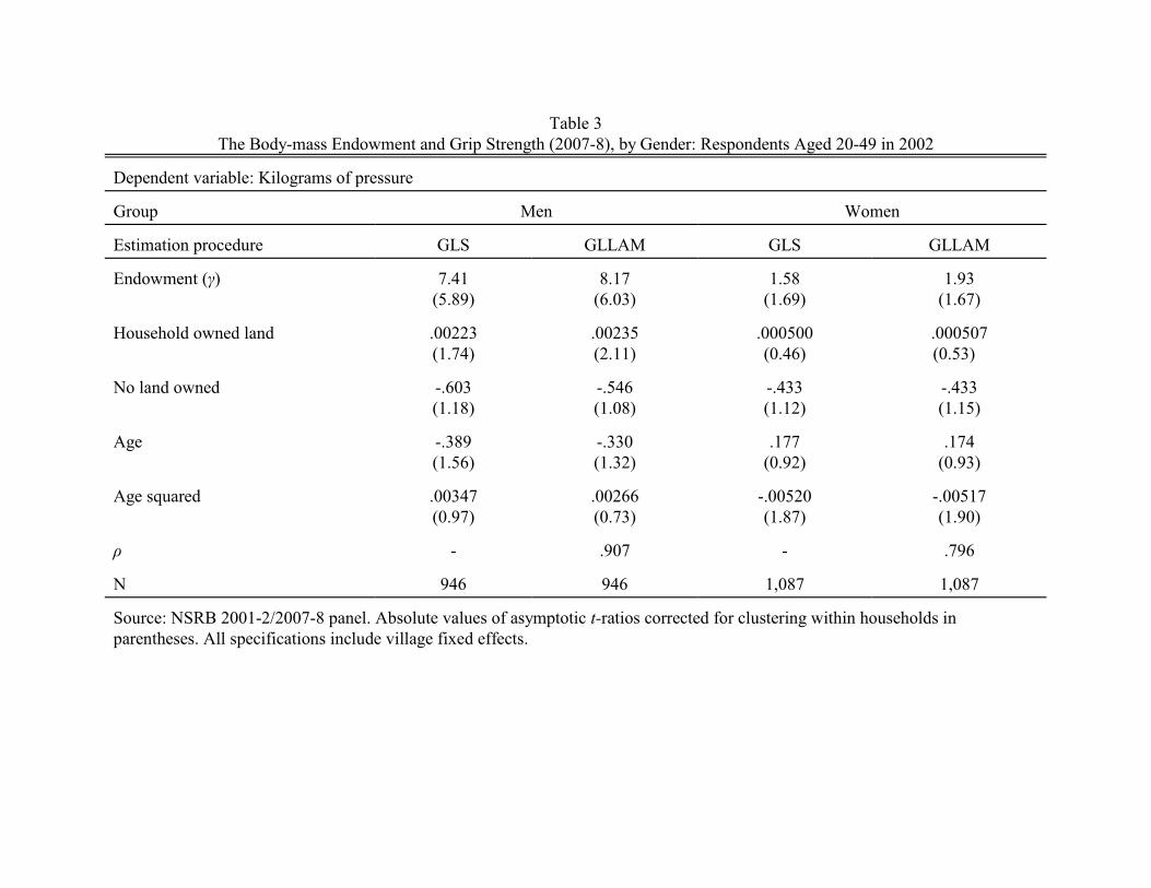
Table 3The Body-mass Endowment and Grip Strength (2007-8), by Gender: Respondents Aged 20-49 in 2002

Dependent variable: Kilograms of pressure

Group Men Women

Estimation procedure GLS GLLAM GLS GLLAM

Endowment (ã) 7.41(5.89)

8.17(6.03)

1.58(1.69)

1.93(1.67)

Household owned land .00223(1.74)

.00235(2.11)

.000500(0.46)

.000507(0.53)

No land owned -.603(1.18)

-.546(1.08)

-.433(1.12)

-.433(1.15)

Age -.389(1.56)

-.330(1.32)

.177(0.92)

.174(0.93)

Age squared .00347(0.97)

.00266(0.73)

-.00520(1.87)

-.00517(1.90)

ñ - .907 - .796

N 946 946 1,087 1,087

Source: NSRB 2001-2/2007-8 panel. Absolute values of asymptotic t-ratios corrected for clustering within households inparentheses. All specifications include village fixed effects.

Table 4Multinomial Logit and Logit-GLLAM Estimates of the Determinants of Children’s Activities:

Children Ages 10-15 in 2001-2 (Left out activity = Schooling)

Estimation method Multinomial Logit ML Logit-GLLAMa b

Activity Work Home Time Work Home Time

Boys

Endowment 2.33(2.42)

.284(0.15)

4.09(3.41)

.426(0.13)

Household land owned -.0599(2.93)

-.0515(1.01)

-.0603(2.94)

-.0515(0.55)

No land owned .356(1.09)

.348(0.45)

.359(1.19)

.344(0.04)

Household average endowment .817(0.57)

1.38(0.58)

.784(0.58)

1.39(0.34)

Age .261(2.82)

.799(2.52)

.254(2.53)

.800(0.16)

N 410 410

Girls

Endowment -5.66(2.62)

1.46(0.89)

-6.87(2.84)

1.72(0.93)

Household land owned .0174(0.84)

-.0386(1.38)

.0157(0.54)

-.0389(1.09)

No land owned .705(1.08)

.607(1.41)

.632(0.88)

.605(1.21)

Household average endowment ofother family members

-1.61(0.90)

-.691(0.47)

-1.94(1.14)

-.642(0.42)

Age -.0178(0.07)

.550(3.18)

-.0994(0.36)

.581(3.06)

N 353 353

Source: NSRB 2001-2. Asymptotic t-ratios corrected for clustering at the household level in columns.a

Bootstrapped t-ratios in parentheses in columns.b

Table 5Estimated Marginal Effects of the Body-Mass Endowment on the Probability of Attending School,

by Gender and Estimation Method: Children Ages 10-15 in 2001-2

Estimation method Multinomial Logit ML Logit-GLLAMa b

Group Boys Girls Boys Girls

Endowment -.248(2.37)

.0600(0.68)

-.436(3.60)

.0983(1.04)

Household land owned .00670(3.23)

.00135(1.14)

.00674(3.42)

.00135(1.11)

No land owned -.0417(1.08)

-.0463(1.64)

-.0420(1.24)

-.0465(1.70)

Household average endowment ofother family members

-.0955(0.62)

.0667(0.87)

-.0927(1.10)

.0784(1.09)

Age -.0332(3.43)

-.0243(2.54)

-.0325(3.23)

-.0236(2.53)

N 410 353 410 353

Source: NSRB 2001-2 and ML Estimates reported in Table 4. Asymptotic t-ratios corrected fora

clustering at the household level in columns. Bootstrapped t-ratios in parentheses in columns. b

Table 6The Body-mass Endowment in 1981-22 and Completed Schooling in 2001-2, by Gender: Respondents Aged 0-15 in 1982

Dependent variable: Completed education (years) in 2001-2

Gender Male Female

Estimation procedure GLS GLLAM GLS GLLAM

Endowment (1981-2) -1.82(2.05)

-2.22(1.94)

1.00(0.86)

.923(0.67)

Age -.164(0.76)

-.161(0.77)

-.110(0.49)

-.123(0.57)

Age squared .00501(0.36)

.00483(0.36)

-.00908(0.60)

-.00787(0.54)

Household owned land (1981-2) .00711(5.49)

.00711(5.66)

.00467(3.05)

.00468(3.17)

No land owned (1981-2) -1.02(1.48)

-1.03(1.54)

-1.05(1.55)

-1.05(1.68)

Average household endowment(1981-2)

.261(0.12)

.270(0.17)

.116(0.06)

.158(0.08)

ñ - .838 - .821

N 311 311 273 273

Source: NSRB 1981-2/2001-2 panel. Absolute values of asymptotic t-ratios corrected for clustering within households inparentheses. All specifications include village fixed effects.

Table 7The Body-mass Endowment and Occupation Choice, by Gender: Respondents Aged 20-49 in 2001-2

Dependent variable: Occupational Energy Expenditure

Group Men Women

Estimation procedure GLS GLLAM GLS GLLAM

Endowment 81.7(14.9)

93.6(11.6)

-5.78(3.62)

-6.78(2.58)

Age .969(0.89)

.957(0.90)

1.05(3.23)

1.06(2.86)

Age squared -.00153(0.10)

-.000825(0.05)

-.0132(2.80)

-.0133(2.63)

Household owned land -.0195(3.13)

-.0212(3.42)

-.000269(0.15)

-.000262(0.18)

No land owned 6.62(2.87)

6.22(2.67)

2.37(3.64)

2.38(3.11)

Average household endowment ofothers (1981-2)

-27.0(4.14)

-29.0(4.53)

-2.02(1.10)

-2.02(.91)

ñ - .901 - .828

N 1,236 1,236 1,338 1,338

Source: NSRB 2001-2. Absolute values of asymptotic t-ratios corrected for clustering within households in parentheses. Allspecifications include village fixed effects.

Table 8The Body-mass Endowment in 1981-2 and Log Wages in 2001-2: Males Aged 0-17 in 1981-2

Dependent variable: Log daily wage in 2002 (tk.)

Estimation procedure GLS GLLAM GLS GLS GLLAM GLLAM-IV

Schooling (2002) - - .0261(2.27)

.0277(2.41)

.0311(3.01)

.0432(2.18)

Endowment (1982) .252(1.21)

.327(2.16)

- .303(1.46)

.370(2.49)

.387(2.39)

Age .100(2.30)

.106(2.73)

.0750(1.90)

.0994(2.33)

.103(2.66)

.100(2.57)

Age squared -.00517(2.08)

-.00536(2.34)

-.00356(1.61)

-.00510(2.08)

-.00527(2.30)

-.00518(2.26)

Household owned land(1982)

.000404(2.03)

.000412(2.51)

- - - -

No land owned (1982) .0528(0.44)

.0607(0.68)

- - - -

Average householdendowment of others (1982)

-.115(0.27)

-.147(0.45)

- - - -

ñ - .838 - - .838 .838

N 225 225 225 225 225 225

Source: NSRB 1981-2/2001-2 panel. Absolute values of asymptotic t-ratios corrected for clustering within households inparentheses in columns 2-6. Bootstrapped t-values in column 7. All specifications include village fixed effects. Instruments for theIV estimates include household owned land, no owned land and the average household endowment of other household members.

Table 9The Body-mass Endowment and Raven’s Matrices Test Performance (2007-8), by Gender: Respondents Aged 20-49 in 2002

Dependent variable: Number of correct answers

Group Men Women

Estimation procedure GLS GLLAM GLLAM GLS GLLAM GLLAM

Endowment -.355(1.05)

-.371(0.96)

-.0251(0.07)

.605(2.14)

.724(1.86)

.347(0.96)

Schooling - - .151(9.92)

- - .180(9.18)

Household owned land .000905(2.52)

.000896(2.55)

.0000958(0.26)

.000561(1.67)

.000561(1.73)

-.000127(0.38)

No land owned -.365(2.63)

-.380(2.77)

-.168(1.31)

-.328(2.83)

-.329(2.80)

-.128(1.13)

Age -.0502(0.73)

-.0475(0.67)

-.0316(0.47)

-.0671(1.16)

-.0682(1.15)

-.0265(0.48)

Age squared .000110(0.11)

.000069(0.07)

-.000031(0.03)

.000429(0.51)

.000561(0.52)

.000112(0.14)

ñ - .872 .872 - .805 .805

N 1,038 1,038 1,038 1,200 1,200 1,200

Source: NSRB 2002-2007 panel. Absolute values of asymptotic t-ratios corrected for clustering within households in parentheses.All specifications include village fixed effects.

Table 10The Body-mass Endowment in 1982 and Age at Menarche Reported in 2001-2, Girls Aged 0-13 in 1982

Dependent variable: Whether age at menarche occurred after age 13, as reported in 2002

Specification (1) (2)

Estimation procedure Logit GLLAM-Logit Logit GLLAM-Logit

Endowment (1982) -2.23(2.11)

-2.81(1.97)

-2.22(2.00)

-2.72(1.85)

Age - - -.132(0.69)

-.119(0.62)

Age squared - - .00710(0.48)

.00586(0.39)

Household owned land (1982) - - -.000785(0.87)

-.000784(0.87)

No land owned (1982) - - .0966(0.20)

.107(0.23)

ñ - .740 - .740

N 216 216 216 216

Source: NSRB 1981-2/2001-2 panel. Absolute values of asymptotic t-ratios corrected for clustering within households inparentheses. All specifications include village fixed effects.

Table 11Occupation-Specific Wage Function Estimates: Men Aged 20-49 in 2001-2

Dependent variable: Log daily wage (tk.)

Estimation procedure GLS GLLAM GLLAM GLLAM-IVa a a b

Schooling .0409(11.6)

.0417(10.1)

.0529(3.34)

.291(2.17)

Schooling x occupationenergy expenditure

- - -.000201(1.85)

-.00222(2.15)

Endowment - .0765(0.84)

-.362(1.05)

-3.10(3.28)

Endowment x occupationenergy expenditure

- - .00358(2.12)

.0216(3.57)

ä - - -.664(7.57)

-1.687(1.98)

Age .0664(3.60)

.0690(3.72)

.0700(3.86)

.0771(3.06)

Age squared -.000854(3.25)

-.000905(3.36)

-.000878(3.37)

-.000884(2.48)

ñ - .889 .888 .888

N 1,094 1,094 1,094 1,094

Source: NSRB 2001-2. Absolute values of asymptotic t-ratios corrected for clustering withina

households in parentheses in column. Bootstrapped t-ratios in parentheses in column.b