human capital formation in childhood and … capital formation in childhood and adolescence flávio...
TRANSCRIPT

Human Capital Formation in Childhood andAdolescence
Flávio Cunha
Rice University
August 7, 2017
Flávio Cunha (Rice University) Human Capital Formation in Childhood and Adolescence August 7, 2017 1 / 186

Evolution of Inequality in USA
Flávio Cunha (Rice University) Human Capital Formation in Childhood and Adolescence August 7, 2017 2 / 186

0.00
0.30
0.60
0.90
1.20
1
FigureRelative Supply and Demand of Skilled Labor
Case 1: Supply and Demand Grow at Same Rate
Relative demand for skilled labor
Relativesupply ofskilledlabor
Relative Skill Premium
Relative stocks of skills

0.00
0.30
0.60
0.90
1.20
1
FigureRelative Supply and Demand of Skilled Labor
Case 1: Supply and Demand Grow at Same Rate
Relative demand for skilled labor
Relativesupply ofskilledlabor
Relative Skill Premium
Relative stocks of skills

0.00
0.30
0.60
0.90
1.20
1
FigureRelative Supply and Demand of Skilled Labor
Case 1: Supply and Demand Grow at Same Rate
Relative demand for skilled labor
Relativesupply ofskilledlabor
Relative Skill Premium
Relative stocks of skills

0.00
0.30
0.60
0.90
1.20
1
FigureRelative Supply and Demand of Skilled Labor
Case 1: Supply and Demand Grow at Same Rate
Relative demand for skilled labor
Relativesupply ofskilledlabor
Relative Skill Premium
Relative stocks of skills
0.00
0.30
0.60
0.90
1.20
1
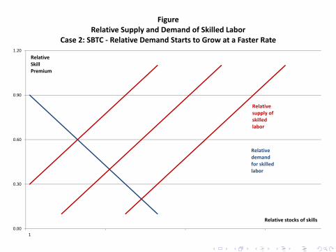
FigureRelative Supply and Demand of Skilled Labor
Case 2: SBTC ‐ Relative Demand Starts to Grow at a Faster Rate
Relativesupply ofskilledlabor
Relative demand for skilled labor
Relative Skill Premium
Relative stocks of skills

0.00
0.30
0.60
0.90
1.20
1
FigureRelative Supply and Demand of Skilled Labor
Case 2: SBTC ‐ Relative Demand Starts to Grow at a Faster Rate
Relativesupply ofskilledlabor
Relative demand for skilled labor
Relative Skill Premium
Relative stocks of skills
0.00
0.30
0.60
0.90
1.20
1
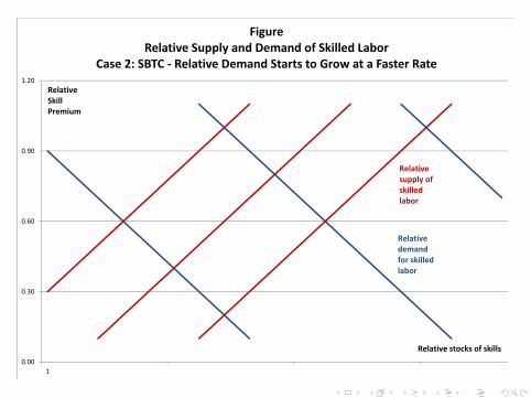
FigureRelative Supply and Demand of Skilled Labor
Case 2: SBTC ‐ Relative Demand Starts to Grow at a Faster Rate
Relativesupply ofskilledlabor
Relative demand for skilled labor
Relative Skill Premium
Relative stocks of skills

0.00
0.30
0.60
0.90
1.20
1
FigureRelative Supply and Demand of Skilled Labor
Case 2: SBTC ‐ Relative Demand Starts to Grow at a Faster Rate
Relativesupply ofskilledlabor
Relative demand for skilled labor
Relative Skill Premium
Relative stocks of skills

0.00
0.30
0.60
0.90
1.20
1
FigureRelative Demand and Supply of Skilled Labor
Case 3: Relative Supply Starts to Grow at Slower Rate
Relativesupply ofskilledlabor
Relative demand for skilled labor
Relative Skill Premium
Relative stocks of skills

0.00
0.30
0.60
0.90
1.20
1
FigureRelative Demand and Supply of Skilled Labor
Case 3: Relative Supply Starts to Grow at Slower Rate
Relativesupply ofskilledlabor
Relative demand for skilled labor
Relative Skill Premium
Relative stocks of skills

0.00
0.30
0.60
0.90
1.20
1
FigureRelative Demand and Supply of Skilled Labor
Case 3: Relative Supply Starts to Grow at Slower Rate
Relativesupply ofskilledlabor
Relative demand for skilled labor
Relative Skill Premium
Relative stocks of skills

0.00
0.30
0.60
0.90
1.20
1
FigureRelative Demand and Supply of Skilled Labor
Case 3: Relative Supply Starts to Grow at Slower Rate
Relativesupply ofskilledlabor
Relative demand for skilled labor
Relative Skill Premium
Relative stocks of skills

Evolution of Inequality in USA
Flávio Cunha (Rice University) Human Capital Formation in Childhood and Adolescence August 7, 2017 15 / 186

Evolution of Inequality in USA
(a)
0
2
4
6
8
10
12
14
16
1900 1910 1920 1930 1940 1950 1960 1970 1980Birth year
Yea
rs o
f ed
ucat
iona
l atta
inm
ent
MaleFemale
(b)
0%
10%
20%
30%
40%
50%
60%
70%
80%
90%
1900 1910 1920 1930 1940 1950 1960 1970 1980Birth year
Sha
re c
ohor
t en
rolli
ng in
col
lege College enrollment, male
College enrollment, female
(c)
0%
5%
10%
15%
20%
25%
30%
35%
40%
45%
1900 1910 1920 1930 1940 1950 1960 1970 1980Birth year
Sha
re c
ohor
t co
mpl
etin
g co
llege
College graduates, maleCollege graduates, female
Figure 8.3 Educational Attainment by Birth Cohort, 1900–1980. (a) Years of Schooling. (b) CollegeEnrollment. (c) College Degree Attainment.
Source: Data are from Goldin and Katz (2008) and tabulated from 1940 to 2000 Census of PopulationIntegrated Public Use Microdata Samples (IPUMS). Observations are for US native-born individualsadjusted to 35 years of age. Figure 8.3a shows the fraction of each birth cohort with at least a high schooldegree, Fig. 8.3b shows the fraction of each cohort with some college attendance, and Fig. 8.3c shows thefraction of each cohort with a college degree. For additional details, see DeLong, Goldin, and Katz (2003).
578 John Bound and Sarah Turner
Flávio Cunha (Rice University) Human Capital Formation in Childhood and Adolescence August 7, 2017 16 / 186

Evolution of Inequality in USA
Comparing across the panels shown in Fig. 8.3, it is clear that changes in collegedegree attainment have not followed changes in college enrollment consistently overthe course of the last 25 years. While college enrollment rates have increased fairly con-sistently, college degree attainment declined before increasing among more recentcohorts. Figure 8.4 presents the trend by birth cohort in the share of enrolled collegestudents who complete a BA degree—essentially the trend shown in Fig. 8.3c dividedby the trend in Fig. 8.3b. For both men and women, the rate of college completion hasbeen below 50% for nearly a half century, with this level appreciably below the rate ofcompletion achieved by men in the early part of the century.
A component of this stagnation has been a growing disparity in college completionrates by parental circumstances. For example, for high school students from the topquartile of the family income distribution, completion rates rose slightly from 67.4 to71% between those starting college in the early 1980s and those starting in the early1990s, while the college completion rates fell for students from other income groups(Bowen, Chingos, and McPherson (2009)). Indeed, for 1992 high school seniors whoenrolled in college, the difference in college completion rates between the students
0%
10%
20%
30%
40%
50%
60%
70%
1900 1910 1920 1930 1940 1950 1960 1970 1980Birth year
Col
lege
com
plet
ion
rate
College graduation rate, maleCollege graduation rate, female
Figure 8.4 Share of College Entrants Receiving BA Degree.
Notes: The completion rate presented in this figure represents the ratio of the number of college degreerecipients (Fig. 8.3c) to the number of individuals with at least some college (Fig. 8.3b). See Fig. 8.3 foradditional notes on the data.
Dropouts and Diplomas 579
Flávio Cunha (Rice University) Human Capital Formation in Childhood and Adolescence August 7, 2017 17 / 186

Evolution of Inequality in USA
Mean SAT/ACT Percentile Score of Colleges, by Colleges' Selectivity in 1962
0
10
20
30
40
50
60
70
80
90
100
1962 1967 1972 1977 1982 1987 1992 1997 2002 2007
Year
Mean SA
T or ACT
Percentile
Score of C
olleges in the
Group
most selective in 1962: 4‐year colleges withselectivity in the 99th %ile in 1962
96th‐98th %ile in 1962
91st‐95th %ile in 1962
81st‐90th %ile in 1962
71st‐80th %ile in 1962
61st‐70th %ile in 1962
51st‐60th %ile in 1962
41st‐50th %ile in 1962
31st‐40th %ile in 1962
21st‐30th %ile in 1962
11th‐20th %ile in 1962
6th‐10th %ile in 1962
least selective in 1962: 4‐year colleges withselectivity in the 1st‐5th %iles in 1962
2 year colleges (estimated)
Figure 1
29
Flávio Cunha (Rice University) Human Capital Formation in Childhood and Adolescence August 7, 2017 18 / 186

Evolution of Inequality in USA
1. Year of reference 2011. Countries are ranked in ascending order of the percentage-point difference between the 25-34 and 55-64 year-old population with tertiary educationSource: OECD. Table A1.3a. See Annex 3 for notes (www.oecd.org/edu/eag.htm ).
Proportion of the 25‐34 year‐old
population with tertiary
education (left axis)
Proportion of the 55‐64 year‐old
population with tertiary
education (left axis)
Difference between the 25‐34 and
55‐64 year‐old population with
tertiary education (right axis)
Israel 44.50 46.52 ‐2.02
United States 44.04 41.81 2.23
Germany 28.96 26.43 2.52
Brazil 14.46 10.17 4.28
Estonia 39.84 35.50 4.34
Austria 23.03 16.73 6.29
Russian Federation 56.97 49.16 7.81
Finland 39.75 31.39 8.36
Chile1 22.48 13.06 9.42
Turkey 21.00 10.32 10.67
Italy 22.25 11.42 10.83
Denmark 40.24 28.67 11.57
Mexico 24.10 12.51 11.59
Switzerland 40.64 28.74 11.90
New Zealand 46.87 34.59 12.28
Canada 57.26 44.49 12.77
Slovak Republic 26.98 13.68 13.30
Iceland 38.38 24.94 13.44
Australia 47.23 33.03 14.20
Greece 34.74 20.04 14.71
Sweden 43.47 28.66 14.82
OECD average 39.20 24.19 15.01
Norway 45.02 29.91 15.11
Hungary 30.43 15.32 15.11
Netherlands 43.04 27.85 15.18
Czech Republic 27.83 12.63 15.20
United Kingdom 47.86 32.62 15.24
Latvia 38.72 22.05 16.68
Portugal 28.33 11.07 17.26
Belgium 42.99 25.34 17.65
Slovenia 35.36 17.14 18.22
Spain 39.26 19.02 20.24
France 42.91 19.60 23.31
Luxembourg 49.88 26.44 23.44
Ireland 49.21 24.86 24.35
Japan 58.55 32.05 26.51
Poland 40.80 12.63 28.17
Korea 65.69 13.54 52.14
Figure 3Percentage of Younger and Older Adults with Tertiary Education
‐10
0
10
20
30
40
50
60
70
‐10
0
10
20
30
40
50
60
70
Israel
United States
German
y
Brazil
Estonia
Austria
Russian Federation
Finland
Chile1
Turkey
Italy
Denmark
Mexico
Switzerlan
d
New
Zealan
d
Can
ada
Slovak Rep
ublic
Iceland
Australia
Greece
Swed
en
OEC
D average
Norw
ay
Hungary
Netherlands
Czech Rep
ublic
United Kingd
om
Latvia
Portugal
Belgium
Slovenia
Spain
Fran
ce
Luxembourg
Irelan
d
Japan
Poland
Korea
Difference between the 25-34 and 55-64 year-old population with tertiary education (right axis)
Proportion of the 25-34 year-old population with tertiary education (left axis)
Proportion of the 55-64 year-old population with tertiary education (left axis)
Perecentage points
Flávio Cunha (Rice University) Human Capital Formation in Childhood and Adolescence August 7, 2017 19 / 186

Simple Model
Let LS and LU denote, respectively, skilled and unskilled labor.Let wS and wU denote, respectively, skilled and unskilled wagerates.Consider the following problem:
minwSLS + wULU
subject to the technology of skill formation:
Y =[γL
φS + (1− γ) L
φU
] 1
φ
where γ ∈ [0, 1] and φ ≤ 1.
Flávio Cunha (Rice University) Human Capital Formation in Childhood and Adolescence August 7, 2017 20 / 186

Simple Model
Taking first-order conditions:
wS = λ[γL
φS + (1− γ) L
φU
] 1−φφ
γLφ−1S
wU = λ[γL
φS + (1− γ) L
φU
] 1−φφ
(1− γ) Lφ−1U
which yields:
lnwS
wU= ln
γ
1− γ+ (φ− 1) ln
LS
LU
Flávio Cunha (Rice University) Human Capital Formation in Childhood and Adolescence August 7, 2017 21 / 186

Evolution of Inequality in USA
Flávio Cunha (Rice University) Human Capital Formation in Childhood and Adolescence August 7, 2017 22 / 186

Model Human Critical Genes Model Est Causality Hetero Age 10 Summary
Figure 1: The Probability of Educational Decisions, by EndowmentLevels, Dropping from Secondary School vs. Graduating
Decile of Cognitive
1 2 3 4 5 6 7 8 9 10
Decile of Socio-Emotional12
34567
8910
Pro
bab
ility
0
0.2
0.4
0.6
0.8
1
Decile of Cognitive
1 2 3 4 5 6 7 8 9 10
Pro
bab
ility
0
0.2
0.4
0.6
0.8
1
Fra
ctio
n
0
0.02
0.04
0.06
0.08
0.1
0.12
0.14
0.16
0.18
0.2
Probability
Decile of Socio-Emotional
1 2 3 4 5 6 7 8 9 10P
rob
abili
ty0
0.2
0.4
0.6
0.8
1
Fra
ctio
n
0
0.02
0.04
0.06
0.08
0.1
0.12
0.14
0.16
0.18
0.2
Probability
Source: Heckman, Humphries, Urzua, and Veramendi (2011).
James Heckman Economics and Econometrics of Human Development

Model Human Critical Genes Model Est Causality Hetero Age 10 Summary
Figure 2: The Probability of Educational Decisions, by EndowmentLevels, HS Graduate vs. College Enrollment
Decile of Cognitive
1 2 3 4 5 6 7 8 9 10
Decile of Socio-Emotional12
34567
8910
Pro
bab
ility
0
0.2
0.4
0.6
0.8
1
Decile of Cognitive
1 2 3 4 5 6 7 8 9 10
Pro
bab
ility
0
0.2
0.4
0.6
0.8
1
Fra
ctio
n
0
0.02
0.04
0.06
0.08
0.1
0.12
0.14
0.16
0.18
0.2
0.22
0.24Probability
Decile of Socio-Emotional
1 2 3 4 5 6 7 8 9 10
Pro
bab
ility
0
0.2
0.4
0.6
0.8
1
Fra
ctio
n
0
0.02
0.04
0.06
0.08
0.1
0.12
0.14
0.16
0.18
0.2
0.22
0.24Probability
Source: Heckman, Humphries, Urzua, and Veramendi (2011).
James Heckman Economics and Econometrics of Human Development

Model Human Critical Genes Model Est Causality Hetero Age 10 Summary
Figure 3: The Probability of Educational Decisions, by EndowmentLevels, Some College vs. 4-year college degree
Decile of Cognitive
1 2 3 4 5 6 7 8 9 10
Decile of Socio-Emotional12
34567
8910
Pro
bab
ility
0
0.2
0.4
0.6
0.8
1
Decile of Cognitive
1 2 3 4 5 6 7 8 9 10
Pro
bab
ility
0
0.2
0.4
0.6
0.8
1
Fra
ctio
n
0
0.05
0.1
0.15
0.2
0.25
0.3
0.35Probability
Decile of Socio-Emotional
1 2 3 4 5 6 7 8 9 10P
rob
abili
ty0
0.2
0.4
0.6
0.8
1
Fra
ctio
n
0
0.05
0.1
0.15
0.2
0.25
0.3Probability
Source: Heckman, Humphries, Urzua, and Veramendi (2011).
James Heckman Economics and Econometrics of Human Development

Model Human Critical Genes Model Est Causality Hetero Age 10 Summary
Figure 4: The Effect of Cognitive and Socio-emotional endowments,(log) Wages
Decile of Cognitive
1 2 3 4 5 6 7 8 9 10
Decile of Socio-Emotional12
34567
8910
Lo
g-w
ages
2.12.22.32.42.52.62.72.82.9
3
Decile of Cognitive
1 2 3 4 5 6 7 8 9 10
Lo
g-w
ages
2.2
2.4
2.6
2.8
3
3.2
Fra
ctio
n
0
0.02
0.04
0.06
0.08
0.1
0.12
0.14
0.16
0.18
0.2
Log-wages
Decile of Socio-Emotional
1 2 3 4 5 6 7 8 9 10L
og
-wag
es2.2
2.4
2.6
2.8
3
3.2
Fra
ctio
n
0
0.02
0.04
0.06
0.08
0.1
0.12
0.14
0.16
0.18
0.2
Log-wages
Source: Heckman, Humphries, Urzua, and Veramendi (2011).
James Heckman Economics and Econometrics of Human Development

Model Human Critical Genes Model Est Causality Hetero Age 10 Summary
Figure 5: The Effect of Cognitive and Socio-emotional endowments,Daily Smoking
Decile of Cognitive
12345678910
Decile of Socio-Emotional
1 2 34 5 6
7 8 910S
mo
ker
0.10.20.30.40.50.60.70.8
Decile of Cognitive
1 2 3 4 5 6 7 8 9 10
Sm
oke
r
0.1
0.2
0.3
0.4
0.5
0.6
0.7
0.8
0.9
Fra
ctio
n
0
0.02
0.04
0.06
0.08
0.1
0.12
0.14
0.16
0.18
0.2
Smoker
Decile of Socio-Emotional
1 2 3 4 5 6 7 8 9 10
Sm
oke
r0.1
0.2
0.3
0.4
0.5
0.6
0.7
0.8
0.9
Fra
ctio
n
0
0.02
0.04
0.06
0.08
0.1
0.12
0.14
0.16
0.18
0.2
Smoker
Source: Heckman, Humphries, Urzua, and Veramendi (2011).
James Heckman Economics and Econometrics of Human Development
Model Human Critical Genes Model Est Causality Hetero Age 10 Summary
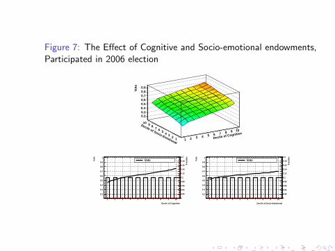
Figure 7: The Effect of Cognitive and Socio-emotional endowments,Participated in 2006 election
Decile of Cognitive
1 2 3 4 5 6 7 8 9 10
Decile of Socio-Emotional12
34567
8910
Vo
te
0.20.30.40.50.60.70.80.9
Decile of Cognitive
1 2 3 4 5 6 7 8 9 10
Vo
te
0.2
0.3
0.4
0.5
0.6
0.7
0.8
0.9
1
Fra
ctio
n
0
0.02
0.04
0.06
0.08
0.1
0.12
0.14
0.16
0.18
0.2
Vote
Decile of Socio-Emotional
1 2 3 4 5 6 7 8 9 10
Vo
te0.2
0.3
0.4
0.5
0.6
0.7
0.8
0.9
1
Fra
ctio
n
0
0.02
0.04
0.06
0.08
0.1
0.12
0.14
0.16
0.18
0.2
Vote
Source: Heckman, Humphries, Urzua, and Veramendi (2011).
James Heckman Economics and Econometrics of Human Development

Model Human Critical Genes Model Est Causality Hetero Age 10 Summary
Figure 8: The Effect of Cognitive and Socio-emotional endowments onProbability of White-collar occupation (age 30)
Decile of Cognitive
1 2 3 4 5 6 7 8 9 10
Decile of Socio-Emotional12
34567
8910
Wh
itec
olla
r
0.10.20.30.40.50.60.70.80.9
1
Decile of Cognitive
1 2 3 4 5 6 7 8 9 10
Wh
itec
olla
r
0.2
0.4
0.6
0.8
1
Fra
ctio
n
0
0.02
0.04
0.06
0.08
0.1
0.12
0.14
0.16
0.18
0.2
Whitecollar
Decile of Socio-Emotional
1 2 3 4 5 6 7 8 9 10
Wh
itec
olla
r
0.2
0.4
0.6
0.8
1
Fra
ctio
n
0
0.02
0.04
0.06
0.08
0.1
0.12
0.14
0.16
0.18
0.2
Whitecollar
Source: Heckman, Humphries, Urzua, and Veramendi (2011).
James Heckman Economics and Econometrics of Human Development

Model Human Critical Genes Model Est Causality Hetero Age 10 Summary
Ever been in jail by age 30, by ability (males)
Polarization
Argument
Skills
Evidence
Critical and Sensitive Periods
Environment
Intuitive
Estimates
Illustration
Summary
.15
.05
.10
.00
NoncognitiveCognitive
0 – 20 21 – 40 41 – 60 61 – 80 81 – 100
Prob
abili
ty
Percentile
Note: This figure plots the probability of a given behavior associated with moving up in one ability distribution for someone after integrating out the other distribution. For example, the lines with markers show the effect of increasing noncognitive ability after integrating the cognitive ability.
Ever Been in Jail by Age 30, by Ability (Males)
Source: Heckman, Stixrud, and Urzua (2006).
Note: This figure plots the probability of a given behavior associated with moving upin one ability distribution for someone after integrating out the other distribution. Forexample, the lines with markers show the effect of increasing socioemotional ability afterintegrating the cognitive ability.
Source: Heckman, Stixrud, and Urzua (2006).
James Heckman Economics and Econometrics of Human Development
Model Human Critical Genes Model Est Causality Hetero Age 10 Summary
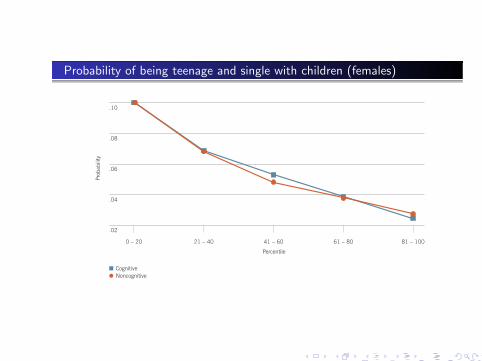
Probability of being teenage and single with children (females)
Polarization
Argument
Skills
Evidence
Critical and Sensitive Periods
Environment
Intuitive
Estimates
Illustration
Summary
Probability of Being Single With Children (Females)
.08
.04
.06
.02
.10
NoncognitiveCognitive
0 – 20 21 – 40 41 – 60 61 – 80 81 – 100
Prob
abili
ty
Percentile
Note: This figure plots the probability of a given behavior associated with moving up in one ability distribution for someone after integrating out the other distribution. For example, the lines with markers show the effect of increasing noncognitive ability after integrating the cognitive ability.
Source: Heckman, Stixrud, and Urzua (2006).
Note: This figure plots the probability of a given behavior associated with moving upin one ability distribution for someone after integrating out the other distribution. Forexample, the lines with markers show the effect of increasing socioemotional ability afterintegrating the cognitive ability.
Source: Heckman, Stixrud, and Urzua (2006).
James Heckman Economics and Econometrics of Human Development

Gaps in Skills in Childhood and AdolescenceCNLSY/79 Data
Introduction Simple Model Structural Model Data and Estimates Conclusion and Future Work
The Gaps in Skill Open Up at Early Ages: Carneiro andHeckman (2002).
-0.8000
-0.6000
-0.4000
-0.2000
0.0000
0.2000
0.4000
0.6000
0.8000
3 5 6 7 8 9 10 11 12 13 14
Age
Bottom Quartile Second Quartile Third Quartile Top Quartile
Flávio Cunha (Rice University) Human Capital Formation in Childhood and Adolescence August 7, 2017 32 / 186

Gaps in Skills in Early ChildhoodHart and Risley (1995)
Flávio Cunha (Rice University) Human Capital Formation in Childhood and Adolescence August 7, 2017 33 / 186
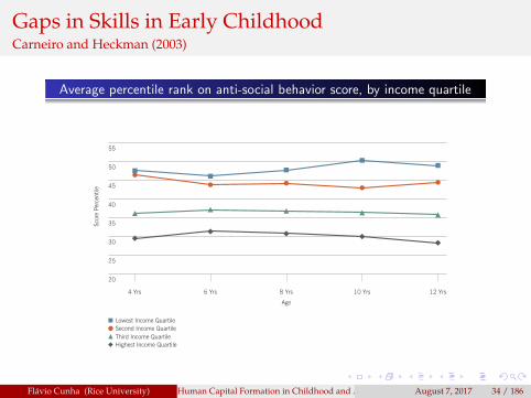
Gaps in Skills in Early ChildhoodCarneiro and Heckman (2003)
Model Human Critical Genes Model Est Causality Hetero Age 10 Summary
Average percentile rank on anti-social behavior score, by income quartile
Polarization
Argument
Skills
Evidence
Critical and Sensitive Periods
Environment
Intuitive
Estimates
Illustration
Summary
Average Percentile Rank on Anti-Social Behavior Score, by Income Quartile
Third Income Quartile
55
30
35
45
40
50
25
20
Second Income Quartile Lowest Income Quartile
Highest Income Quartile
4 Yrs 6 Yrs 12 Yrs
Scor
e Pe
rcen
tile
8 Yrs 10 Yrs
Age
James Heckman Economics and Econometrics of Human Development
Flávio Cunha (Rice University) Human Capital Formation in Childhood and Adolescence August 7, 2017 34 / 186

Gaps in Skills in Early ChildhoodCasey, Lubotsky, and Paxson (2002)
Model Human Critical Genes Model Est Causality Hetero Age 10 Summary
Health and income for children and adults, U.S. National Health Interview Survey
1986-1995.∗
)emocniylimaf(nl110198
5.1
57.1
2
52.2
3-0sega
8-4sega
21-9sega
71-31sega
heal
thsta
tus(
1 =
exce
llent
to5
= po
or)
∗ From Case, A., Lubotsky, D. & Paxson, C. (2002), American Economic Review, Vol. 92, 1308-1334.
James Heckman Economics and Econometrics of Human Development
Flávio Cunha (Rice University) Human Capital Formation in Childhood and Adolescence August 7, 2017 35 / 186

Gaps in Investments in Early ChildhoodCarneiro and Heckman (2003)Inequality in Skills are Partially the Result of Inequality in
Investments: Cunha (2007)
FigureUnadjusted Mean Home Score
by Quartile of Permanent Income of the Family
7 6
7.8
by Quartile of Permanent Income of the Family
7.4
7.6
7.0
7.2
6.6
6.8
6.2
6.4
6.2
0 1‐2 3‐4 5‐6 7‐8 9‐10 11‐12 13‐14
Bottom Quartile 2nd Quartile 3rd Quartile Top QuartileFlávio Cunha and Anton Badev University of Pennsylvania () 10/17 6 / 44
Flávio Cunha (Rice University) Human Capital Formation in Childhood and Adolescence August 7, 2017 36 / 186

Gaps in Investments in Early ChildhoodHart and Risley (1995)
Flávio Cunha (Rice University) Human Capital Formation in Childhood and Adolescence August 7, 2017 37 / 186

Gaps in Investments in Early ChildhoodPSID, CDS
0.2
.4.6
.8
0 1 2 3 4 5Investments (hours per day)
kdensity Bottom kdensity Second
kdensity Third kdensity Top
by Quartiles of Permanent IncomeInvestments in Human Capital of Children
Flávio Cunha (Rice University) Human Capital Formation in Childhood and Adolescence August 7, 2017 38 / 186

Gaps in Investments in Early ChildhoodKalil, Ryan, and Corey (2012)
Figure 3: Education gradient in play time. Source: Kalil, A., Ryan, R., & Corey, M. (2012). Diverging destinies: Maternal education and the developmental gradient in time with children. Demography, 49, 1361-1383.
0.00
10.00
20.00
30.00
40.00
50.00
60.00
70.00
80.00
0‐2 3‐5 6‐13
Minutes in
Play
Child Age
College or Beyond
Some College
HS
< HS
Flávio Cunha (Rice University) Human Capital Formation in Childhood and Adolescence August 7, 2017 39 / 186

Gaps in Investments in Early ChildhoodKalil, Ryan, and Corey (2012)
0.00
2.00
4.00
6.00
8.00
10.00
12.00
14.00
16.00
0‐2 3‐5 6‐13
Minutes in
Teaching
Child Age
College or Beyond
Some College
HS
< HS
Figure 4: Education gradient in teaching time. Source: Kalil, A., Ryan, R., & Corey, M. (2012). Diverging destinies: Maternal education and the developmental gradient in time with children. Demography, 49, 1361-1383.
Flávio Cunha (Rice University) Human Capital Formation in Childhood and Adolescence August 7, 2017 40 / 186

Gaps in Investments in AdolescenceKalil, Ryan, and Corey (2012)
0.00
5.00
10.00
15.00
20.00
25.00
30.00
0‐2 3‐5 6‐13
Minutes in
Managem
ent
Child Age
College or Beyond
Some College
HS
< HS
Figure 5: Education gradient in management time. Source: Kalil, A., Ryan, R., & Corey, M. (2012). Diverging destinies: Maternal education and the developmental gradient in time with children. Demography, 49, 1361-1383.
Flávio Cunha (Rice University) Human Capital Formation in Childhood and Adolescence August 7, 2017 41 / 186

Model Human Critical Genes Model Est Causality Hetero Age 10 Summary
Figure 15: Parental Investment over Childhood among Whites byMother’s Education: Material Resources
0.2
.4.6
Sco
re
4 6 8 10 12 14Age
Less than HS HS More than HS
Data: A balanced panel from Children of National Longitudinal Survey of Youth 1979.
Source: Moon (2012).
James Heckman Economics and Econometrics of Human Development

Model Human Critical Genes Model Est Causality Hetero Age 10 Summary
Figure 16: Parental Investment over Childhood among Whites byMother’s Education: Cognitive Stimulation
−.2
0.2
.4.6
Sco
re
4 6 8 10 12 14Age
Less than HS HS More than HS
Data: A balanced panel from Children of National Longitudinal Survey of Youth 1979.
Source: Moon (2012).
James Heckman Economics and Econometrics of Human Development

Model Human Critical Genes Model Est Causality Hetero Age 10 Summary
Figure 17: Parental Investment over Childhood among Whites byMother’s Education: Emotional Support
0.0
5.1
.15
.2.2
5S
core
4 6 8 10 12 14Age
Less than HS HS More than HS
Data: A balanced panel from Children of National Longitudinal Survey of Youth 1979.
Source: Moon (2012).
James Heckman Economics and Econometrics of Human Development

Model Human Critical Genes Model Est Causality Hetero Age 10 Summary
Figure 18: Parental Investment over Childhood among Whites by FamilyIncome Quartile: Cognitive Stimulation
0.2
.4.6
Sco
re
4 6 8 10 12 14Age
Income Q1 Income Q2 Income Q3 Income Q4
Data: A balanced panel from Children of National Longitudinal Survey of Youth 1979.
Source: Moon (2012).
James Heckman Economics and Econometrics of Human Development

Model Human Critical Genes Model Est Causality Hetero Age 10 Summary
Figure 19: Parental Investment over Childhood among Whites by FamilyType: Cognitive Stimulation
−.2
0.2
.4.6
Sco
re
4 6 8 10 12 14Age
Never−married Single Mom Broken/Blended Intact
Data: A balanced panel from Children of National Longitudinal Survey of Youth 1979.
Source: Moon (2012).
James Heckman Economics and Econometrics of Human Development

The Role of Schools: Araujo et al (2015)
How much, and in what ways, do kindergarten teachers matterfor learning outcomes?Two challenges:
Sorting of students to teachers.
Solution: Randomly match students to teachers.
Data on teachers are weakly correlated with student gain.
Improve the quality of data on teachers.
Flávio Cunha (Rice University) Human Capital Formation in Childhood and Adolescence August 7, 2017 47 / 186

What is the CLASS and why use it? Classroom observa@on tool
Climate (positive or negative), teacher sensitivity, and regard for student perspectives
Emotional support
Behavior management, productivity, and instructional and learning formats Classroom
organization
Concept development, quality of feedback, and language modeling
Instructional support
17

Behavior Management Encompasses the teacher's ability to provide clear behavioral expectations and use effective methods to
prevent and redirect misbehavior. Low (1,2) Mid (3,4,5) High (6,7)
Clear Behavior Expectations Rules and expectations
are absent, unclear, or inconsistently enforced.
Rules and expectations may be stated clearly, but are inconsistently enforced.
Rules and expectations for behavior are clear and are consistently enforced.
▪ Clear expectations ▪ Consistency ▪ Clarity of rules
Proactive
Teacher is reactive and monitoring is absent or ineffective.
Teacher uses a mix of proactive and reactive responses; sometimes monitors but at other times misses early indicators of problems.
Teacher is consistently proactive and monitors effectively to prevent problems from developing.
▪ Anticipates problem behavior or escalation
▪ Rarely reactive ▪ Monitoring
Redirection of Misbehavior
Attempts to redirect misbehavior are ineffective; teacher rarely focuses on positives or uses subtle cues. As a result, misbehavior continues/escalates and takes time away from learning.
Some attempts to redirect misbehavior are effective; teacher sometimes focuses on positives and uses subtle cues. As a result, there are few times when misbehavior continue/escalate or takes time away from learning.
Teacher effectively redirects misbehavior by focusing on positives and making use of subtle cues. Behavior management does not take time away from learning.
▪ Effectively reduces misbehavior ▪ Attention to the positive ▪ Uses subtle cues to redirect ▪ Efficient
Student Behavior There are frequent instances of misbehavior in the classroom.
There are periodic episodes of misbehavior in the classroom.
There are few, if any, instances of student misbehavior in the classroom.
▪ Frequent compliance ▪ Little aggression & defiance Source: Pianta, La Paro & Hamre (2008)
Example: Teacher Behaviors and CLASS Scores for Behavior Management Dimension

The Role of Schools: Araujo et al (2015)
Break analysis in two parts:
Estimate teacher effects: How much does it matter whether a childwas assigned to teacher A or B in a school?Estimate the associations between within-school differences inteacher characteristics or behaviors and child learning outcomes
Flávio Cunha (Rice University) Human Capital Formation in Childhood and Adolescence August 7, 2017 50 / 186
The Role of Schools: Araujo et al (2015)
One standard error in teacher quality leads to increases in childlearning of
11% of standard deviation in math.13% of standard deviation in language.7% of standard deviation in executive function.
Same teachers have their students learn more math and morelanguage year after year.
Cross-year correlation of teacher effects in math is 0.32Cross-year correlation of teacher effects in language is 0.42.
Flávio Cunha (Rice University) Human Capital Formation in Childhood and Adolescence August 7, 2017 51 / 186

The Role of Schools: Araujo et al (2015)
What explains differences in teacher effectiveness?
One standard deviation in teacher IQ increases child’s performanceby 4% of a standard deviation.Students randomly assigned to “rookie” teachers learn 16% ofstandard deviation less.No correlation between teacher personality scores (Big Five) andstudent learning.One standard deviation in CLASS explains 59% of a standarddeviation in student learning.Teachers with better CLASS scores get all their students to learnmore: Effects are not concentrated on girls or boys, on childrenwith high or low levels of development when they enter school, oron children of high or low socioeconomic status
Flávio Cunha (Rice University) Human Capital Formation in Childhood and Adolescence August 7, 2017 52 / 186

The Role of Schools: Araujo et al (2015)
Interestingly, parental reports of teacher quality correlate (veryimperfectly) with teacher effectiveness:
Teachers who produce one standard deviation more learning aregiven a 0.44 higher score (on a scale from 1 to 5).Rookie teachers are given 0.33 lower score by parents.Teachers with higher CLASS scores also get higher scores reportedby parents.
However, parents do not adjust behaviors in response todifferences in teacher quality.
There is no effect on the quality or quantity of parent-childinteraction at home.There is no effect on the child’s dropping out or absenteeism.
Flávio Cunha (Rice University) Human Capital Formation in Childhood and Adolescence August 7, 2017 53 / 186


Model Human Critical Genes Model Est Causality Hetero Age 10 Summary
Figure 22: Causal Effect of Schooling on ASVAB Measures of Cognition
Notes: Effect of schooling on components of the ASVAB. The first four components are averaged to create male’s withaverage ability. We standardize the test scores to have within-sample mean zero, variance one. The model is estimated usingthe NLSY79 sample. Solid lines depict average test scores, and dashed lines, confidence intervals.Source: Heckman, Stixrud and Urzua [2006, Figure 4].
James Heckman Economics and Econometrics of Human Development

Model Human Critical Genes Model Est Causality Hetero Age 10 Summary
Figure 23: Causal Effect of Schooling on Two Measures of Personality
Source: Heckman, Stixrud and Urzua [2006, Figure 5].
James Heckman Economics and Econometrics of Human Development

Increasing Inequality in SkillsReardon (2013)
Figure 1: Trends in race and income achievement gaps, 1943-2001 Cohorts. Source: Reardon, S. (2011). The widening academic achievement gap between the rich and the poor: New evidence and possible explanations. In G. Duncan & R. Murnane (Eds.). Whither Opportunity? Rising Inequality, Schools, and Children's Life Chances (pp. 91-116). New York: Russell Sage Foundation and Spencer Foundation.
Flávio Cunha (Rice University) Human Capital Formation in Childhood and Adolescence August 7, 2017 60 / 186

Increasing Inequality in Skills
Flávio Cunha (Rice University) Human Capital Formation in Childhood and Adolescence August 7, 2017 61 / 186

Trends in Health: Child obesity
Flávio Cunha (Rice University) Human Capital Formation in Childhood and Adolescence August 7, 2017 62 / 186

Increasing Inequality in InvestmentsAltintas (2016)
Flávio Cunha (Rice University) Human Capital Formation in Childhood and Adolescence August 7, 2017 63 / 186

Increasing Inequality in InvestmentsKornrich and Furstenberg (2011)
Figure 7: Enrichment expenditures on children, 1972-2006 (in $2008). Source: Kornrich, S., & Furstenberg, F. (2013). Investing in children: Changes in spending on children, 1972 to 2007. Demography, 50, 1-23.Flávio Cunha (Rice University) Human Capital Formation in Childhood and Adolescence August 7, 2017 64 / 186

Increasing Inequality in Investments
Flávio Cunha (Rice University) Human Capital Formation in Childhood and Adolescence August 7, 2017 65 / 186

Increasing Inequality in Investments
Flávio Cunha (Rice University) Human Capital Formation in Childhood and Adolescence August 7, 2017 66 / 186

Full Circle: College Attendance
Flávio Cunha (Rice University) Human Capital Formation in Childhood and Adolescence August 7, 2017 67 / 186

Full Circle: College Graduation
Flávio Cunha (Rice University) Human Capital Formation in Childhood and Adolescence August 7, 2017 68 / 186

Full Circle: Transition to College
Flávio Cunha (Rice University) Human Capital Formation in Childhood and Adolescence August 7, 2017 69 / 186

Full Circle: Transition to College
Flávio Cunha (Rice University) Human Capital Formation in Childhood and Adolescence August 7, 2017 70 / 186

Full Circle: Transition to College
Flávio Cunha (Rice University) Human Capital Formation in Childhood and Adolescence August 7, 2017 71 / 186

Evidence is Reinforced from Evidence from RCT
Early interventions:Perry Preschool ProgramAbecedarianInfant Health and Development Program (IHDP)Head Start
Interventions at School AgeMontreal Longitudinal Study
Flávio Cunha (Rice University) Human Capital Formation in Childhood and Adolescence August 7, 2017 72 / 186

Early Childhood Education: Elango, Garcia,Heckman, and Hojman (2015)
Table 4: Treatment Effects on Early-life Skills for Samples Pooled Across Gender
Treatment Effect Permutation, one-sided Permutation, two-sided Stepdown, one-sided Stepdown, two-sided
Perry IQ, Age 5 11.422 0.000 0.000 0.000 0.000IQ, Age 8 1.254 0.080 0.430 0.080 0.430Achievement Test Score, Ages 5–10 0.394 0.000 0.000 0.010 0.010Conscientiousness, Ages 4–7 0.273 0.040 0.060 0.050 0.070Achievement Test Score, Age 27 1.795 0.020 0.070 0.080 0.060
ABC IQ, Age 5 6.398 0.030 0.030 0.030 0.030IQ, Age 8 4.500 0.080 0.080 0.180 0.180Achievement Test Score Ages 5–10 0.544 0.010 0.010 0.020 0.020Conscientiousness Ages 4–7 0.047 0.400 0.680 0.860 0.890Achievement Test Score, Age 21 0.422 0.010 0.010 0.120 0.120
IHDP IQ, Age 3 8.475 0.000 0.000 0.000 0.000IQ, Age 8 -0.671 0.680 0.420 0.910 0.430Achievement Test Score, Ages 5–10 -0.012 0.570 0.840 0.830 0.870Conscientiousness, Ages 4–7 0.075 0.060 0.140 0.180 0.190Achievement Test Score, Age 18 0.108 0.470 0.950 0.730 0.930
ETP IQ, Age 7 6.343 0.020 0.080 0.050 0.050IQ, Age, 8 5.743 0.100 0.240 0.150 0.200Achievement Test Score, Ages 5–10 0.534 0.380 0.820 0.510 0.800
Source: Own calculations. Note: Initial sample sizes are: PPP: 123; ABC: 122; IHDP: 985; ETP: 91. Non-parametric permutation p− values account for compromisedrandomization, small sample size, and item non-response. See Heckman et al. (2010a) and Campbell et al. (2014, appendix) for details. Stepdown p − value accountsfor the same and for multiple hypotheses testing. All school-age and adult achievement and conscientiousness measures have mean 0 and standard deviation 1. All IQmeasures have mean 100 and standard deviation 15 and they are standardized using the national population mean and standard deviation. For PPP, IHDP, and ETP atages 5, 3, and 7 we use the Stanford-Binet IQ test. For ABC at 5 we use the Wechsler Preschool and Primary Scale of Intelligence. For PPP and ETP at age 8 we usethe Stanford-Binet IQ test. At this same age, we use Wechsler Intelligence Scale for Children for ABC and IHDP. School Age Achievement is a factor measured througha factor of items at ages 5, 6, and 7. The items analyzed come from the California Achievement Test (ABC, PPP); Metropolitan Achievement Test (ETP); PeabodyIndividual Achievement Test (ABC); Woodcock-Johnson Test of Achievement (ABC, IHDP). School Age Conscientiousness is a factor constructed through a battery ofitems from various questionnaires: Achenbach Child Behavior Checklist (ABC); Classroom Behavior Inventory (ABC); Walker Problem Behavior Identification Checklist(ABC); Teacher rating (PPP, IHDP); Reputation test (PPP, IHDP). Adult achievement is measured by Adult Performance Level (PPP); WoodcockJohnson Test (ABC);Wechsler Adult Intelligence Scale (IHDP). Adult achievement and conscientiousness measures are not available in ETP.
28
Flávio Cunha (Rice University) Human Capital Formation in Childhood and Adolescence August 7, 2017 73 / 186

Early Childhood Education: Elango, Garcia,Heckman, and Hojman (2015)
Table 5: Treatment Effects on Early-life Skills for Females
Treatment Effect Permutation, one-sided Permutation, two-sided Stepdown, one-sided Stepdown, two-sided
Perry IQ, Age 5 12.666 0.000 0.000 0.000 0.000IQ, Age 8 4.240 0.410 0.900 0.700 0.940Achievement Test Score, Ages 5–10 0.564 0.180 0.400 0.300 0.390Conscientiousness, Ages, 4–7 0.515 0.380 0.850 0.610 0.860Achievement Test Score, Age 27 0.407 0.110 0.390 0.330 0.430
ABC IQ, Age 5 3.051 0.050 0.050 0.060 0.060IQ, Age 8 4.573 0.110 0.150 0.360 0.360Achievement Test Score, Ages 5–10 0.822 0.260 0.280 0.410 0.410Conscientiousness, Ages 4–7 0.110 0.600 0.960 0.910 0.960Achievement Test Score, Age 21 0.737 0.240 0.600 0.790 0.840
IHDP IQ Age 3 9.877 0.000 0.000 0.000 0.000IQ Age 8 -0.158 0.780 0.490 0.940 0.600Achievement Test Score Ages 5–10 -0.034 0.500 0.920 0.790 0.970Conscientiousness, Ages 4–7 0.089 0.240 0.440 0.500 0.530Achievement Test Score, Age 18 0.517 0.650 0.790 0.840 0.910
ETP IQ, Age 7 8.611 0.120 0.140 0.180 0.180IQ, Age 8 9.056 0.290 0.540 0.440 0.550Achievement Test Score, Ages 5–10 0.448 0.810 0.350 0.980 0.270
Source: Own calculations. See notes in Table 4.
29
Flávio Cunha (Rice University) Human Capital Formation in Childhood and Adolescence August 7, 2017 74 / 186

Early Childhood Education: Elango, Garcia,Heckman, and Hojman (2015)
Table 6: Treatment Effects on Early-life Skills for Males
Treatment Effect Permutation, one-sided Permutation, two-sided Stepdown, one-sided Stepdown, two-sided
Perry IQ, Age 5 10.607 0.000 0.000 0.010 0.010IQ, Age 8 -0.721 0.060 0.250 0.150 0.190Achievement Test Score, Ages 5–10 0.269 0.000 0.020 0.050 0.050Conscientiousness, Ages4–7 0.087 0.030 0.040 0.040 0.040Achievement Test Score, Age 27 0.214 0.110 0.230 0.160 0.200
ABC IQ, Age 5 9.962 0.530 0.540 0.890 0.890IQ, Age 8 4.174 0.410 0.410 0.760 0.760Achievement Test Score, Ages 5–10 0.277 0.010 0.010 0.030 0.030Conscientiousness, Ages 4–7 0.009 0.590 0.690 0.980 0.980Achievement Test Score, Age 21 0.095 0.070 0.070 0.120 0.120
IHDP IQ, Age 3 6.988 0.000 0.000 0.000 0.000IQ, Age 8 -1.206 0.450 0.930 0.810 0.950Achievement Test Score Ages 5–10 0.012 0.720 0.650 0.900 0.740Conscientiousness, Ages4–7 0.065 0.090 0.170 0.250 0.270Achievement Test Score, Age18 -0.456 0.500 0.820 0.710 0.840
ETP IQ, Age 7 4.111 0.100 0.200 0.160 0.170IQ, Age 8 2.333 0.140 0.210 0.260 0.280Achievement Test Score, Ages 5–10 -0.795 0.180 0.280 0.260 0.280
Source: Own calculations. See notes in Table 4.
30
Flávio Cunha (Rice University) Human Capital Formation in Childhood and Adolescence August 7, 2017 75 / 186

Early Childhood Education: Elango, Garcia,Heckman, and Hojman (2015)
Figure 2: Dynamics of IQ in PPP
(a) Standardized IQ
80
85
90
95
Nu
mb
er
of
Co
rre
ct
An
sw
ers
36 48 60 72 84 96 108 120 132 144Age (Months)
Treated Control
(b) Raw IQ
40
60
80
10
01
20
Nu
mb
er
of
Co
rre
ct
An
sw
ers
36 48 60 72 84 96 108 120 132 144Age (Months)
Treated Control
Source: Reproduced from Hojman (2015). Note: The solid line represents the trajectory of the treatedgroup, and the dotted line represents the trajectory of the control group. Thin lines surroundingtrajectories are asymptotic standard errors. It shows standardized IQ as measured by the Stanford-Binettest in each year. IQ is age-standardized based on a national sample to have a US national mean of 100points and standard deviation of 15 points. In Figure 2b, the scores are not standardized. The scores in itrepresent the raw scores, or the sum of the number of correct questions in each year.
Differences by Gender
A consistent finding across all four programs is the difference in treatment effects for males
and females. This difference is substantial enough to create important gender differences
in both benefit-cost ratios and internal rates of return for PPP and ABC. This pattern is
consistent with the literature on differences in development between girls and boys.40 Girls
develop earlier. Uniform curricula across genders appears to benefit the laggard boys on
many dimensions, but girls benefit as well, as we document in our discussion of the long-
term treatment effects of ABC and PPP. In addition, all programs (except IHDP) target
ages 3–4 when aggressive behavior that predicts adult aggression and participation in crime
begins to manifest itself (White et al., 1994). Gender-specific curricula in preschool may be
an appropriate strategy.
40Lavigueur et al. (1995); Kerr et al. (1997); Masse and Tremblay (1997); Nagin and Tremblay (2001);Bertrand and Pan (2011).
33
Flávio Cunha (Rice University) Human Capital Formation in Childhood and Adolescence August 7, 2017 76 / 186

Early Childhood Education: Elango, Garcia,Heckman, and Hojman (2015)
that persist into adulthood. Non-cognitive outcomes are notably absent due to lack of data.
In PPP and ABC, and for early education programs in general, non-cognitive skills are not
typically followed in the long term.
Table 7: Life-Cycle Outcomes, PPP and ABC
PPP ABCAge Female Male Age Female Male
Cognition and EducationAdult IQ - - - 21c 10.275 2.588
- - - (0.005) (0.130)
High School Graduation 19a 0.56 0.02 21c 0.238 0.176(0.000) (0.416) (0.090) (0.100)
EconomicEmployed 40a -0.01 .29 30c 0.147 0.302
(0.615) (0.011) (0.135) (0.005)
Yearly Labor Income, 2014 USD 40a $6,166 $8,213 30c $3,578 $17,214(0.224) (0.150) (0.000) (0.110)
HI by Employer 40a 0.129 0.206 31b 0.043 0.296(0.055) (0.103) (0.512) (0.035)
Ever on Welfare 18–27a -0.27 0.03 30c 0.006 -0.062(0.049) (0.590) (0.517) (0.000)
CrimeNo. of Arrestsd ≤40a -2.77 -4.88 ≤34c -5.061 -6.834
(0.041) (0.036) (0.051) (0.187)
No. of Non-Juv. Arrests ≤40a -2.45 -4.85 ≤34c -4.531 -6.031One-sided permutation (0.051) (0.025) (0.061) (0.181)
LifestyleSelf-reported Drug User - - - 30c 0.031 -0.438- - - - (0.590) (0.030)
Not a Daily Smoker 27a 0.111 0.119 - - -(0.110) (0.089) - - -
Not a Daily Smoker 40a 0.067 0.194 - - -(0.206) (0.010) - - -
Physical Activity 40a 0.330 0.090 21b 0.249 0.084(0.002) (0.545) (0.004) (0.866)
HealthObesity (BMI >30) - - - 30–34c 0.221 -0.292
- - - (0.920) (0.060)
Hypertension I - - - 30–34c 0.096 0.339- - - (0.380) (0.010)
Source: a Heckman et al. (2010a). b Campbell et al. (2014). c Elango et al. (2015). Note: This table displaysstatistics for the treatment effects of PPP and ABC on important life-cycle outcome variables. HypertensionI is the first stage of high blood pressure—systolic blood pressure between 140 and 159 and diastolic pressurebetween 90 and 99. “HI by employer” refers to health insurance provided by the employer and is conditional
on being employed. d “No. of Arrests” includes offenses in the case of ABC, even where more than one of-fense was charged per arrest. For the further definitions of the outcomes, see the respective web appendicesof the cited papers. Outcomes from Heckman et al. (2010a) are reported with one-sided p − value which isbased on Freedman-Lane procedure, using the linear covariates of maternal employment, paternal presenceand SB (Stanford-Binet) IQ, and restricting permutation orbits within strata formed by a Socio-economicStatus index being above or below the sample median and permuting siblings as a block. p− values for theoutcomes from Campbell et al. (2014) are one-sided single hypothesis constrained permutation p − value’s,based on the IPW (Inverse Probability Weighting) t-statistic associated with the difference in means be-tween treatment groups; probabilities of IPW are estimated using the variables gender, presence of father inhome at entry, cultural deprivation scale, child IQ at entry (SB), number of siblings and maternal employ-ment status. p − values for the outcomes from Elango et al. (2015) are bootstrapped with 1000 resamples,corrected for attrition with Inverse Probability Weights, with treatment effects conditioned on treatmentstatus, cohort, number of siblings, mothers IQ, and the ABC high risk index.
35
Flávio Cunha (Rice University) Human Capital Formation in Childhood and Adolescence August 7, 2017 77 / 186

Early Childhood Education: Elango, Garcia,Heckman, and Hojman (2015)
Figure 3: Decompositions of Treatment Effects of PPP on Male Adult Outcomes
0.056
0.149
0.077
0.161
0.085
0.136
0.046
0.089
0.062
0.071
0.071 0.557
0.403
0.086
0.013
0.018
0.204
0.088
0.141
0.027
0.144
0.246
0.114
0% 20% 40% 60% 80% 100%
Employed, age 40 (0.200**)
# of lifetime arrests, age 40 (-4.20*)
# of adult arrests (misd.+fel.), age 40 (-4.26**)
# of felony arrests, age 40 (-1.14*)
# of misdemeanor arrests, age 40 (-3.13**)
Use tobacco, age 27 (-0.119*)
Monthly income, age 27 (0.876**)
# of adult arrests (misd.+fel.), age 27 (-2.33**)
# of felony arrests, age 27 (-1.12)
# of misdemeanor arrests, age 27 (-1.21**)
CAT total at age 14, end of grade 8 (0.566*)
Cognitive Factor Externalizing Behavior Academic Motivation Other Factors
Source: Reproduced from Heckman et al. (2013). Note: The total treatment effects are shown inparentheses. Each bar represents the total treatment effect normalized to 100 percent. One-sidedp− values are shown above each component of the decomposition. See the Web Appendix of Heckmanet al. (2013) for detailed information about the simplifications made to produce the figure. “CAT total”denotes California Achievement Test total score normalized to control mean 0 and variance of 1. Asterisksdenote statistical significance: * – 10% level; ** – 5% level; *** – 1% level. Monthly income is adjusted tothousands of 2006 dollars using annual national CPI.
Figure 4: Decompositions of Treatment Effects of PPP on Female Adult Outcomes
0.224
0.057
0.046
0.066
0.269
0.339
0.120
0.099
0.199
0.497
0.344
0.256
0.042
0.283
0.533
0.185
0.528
0.050
0.352
0.320
0.369
0.371
0.150
0.127
0.319
0.305
0.109
0.153
0.071
0.228
0.232
0% 20% 40% 60% 80% 100%
Months in all marriages, age 40 (39.6*)
# of lifetime violent crimes, age 40 (-0.574**)
# of felony arrests, age 40 (-0.383**)
# of misdemeanor violent crimes, age 40 (-0.537**)
Ever tried drugs other than alcohol or weed, age 27 (-0.227**)
Jobless for more than 1 year, age 27 (-0.292*)
# of felony arrests, age 27 (-0.269**)
# of misdemeanor violent crimes, age 27 (-0.423**)
Mentally impaired at least once, age 19 (-0.280**)
Any special education, age 14 (-0.262**)
CAT total, age 14 (0.806**)
CAT total, age 8 (0.565*)
Cognitive Factor Externalizing Behavior Academic Motivation Other Factors
Source: Reproduced from Heckman et al. (2013). See note in Figure 3.
37
Flávio Cunha (Rice University) Human Capital Formation in Childhood and Adolescence August 7, 2017 78 / 186

Early Childhood Education: Elango, Garcia,Heckman, and Hojman (2015)
Figure 3: Decompositions of Treatment Effects of PPP on Male Adult Outcomes
0.056
0.149
0.077
0.161
0.085
0.136
0.046
0.089
0.062
0.071
0.071 0.557
0.403
0.086
0.013
0.018
0.204
0.088
0.141
0.027
0.144
0.246
0.114
0% 20% 40% 60% 80% 100%
Employed, age 40 (0.200**)
# of lifetime arrests, age 40 (-4.20*)
# of adult arrests (misd.+fel.), age 40 (-4.26**)
# of felony arrests, age 40 (-1.14*)
# of misdemeanor arrests, age 40 (-3.13**)
Use tobacco, age 27 (-0.119*)
Monthly income, age 27 (0.876**)
# of adult arrests (misd.+fel.), age 27 (-2.33**)
# of felony arrests, age 27 (-1.12)
# of misdemeanor arrests, age 27 (-1.21**)
CAT total at age 14, end of grade 8 (0.566*)
Cognitive Factor Externalizing Behavior Academic Motivation Other Factors
Source: Reproduced from Heckman et al. (2013). Note: The total treatment effects are shown inparentheses. Each bar represents the total treatment effect normalized to 100 percent. One-sidedp− values are shown above each component of the decomposition. See the Web Appendix of Heckmanet al. (2013) for detailed information about the simplifications made to produce the figure. “CAT total”denotes California Achievement Test total score normalized to control mean 0 and variance of 1. Asterisksdenote statistical significance: * – 10% level; ** – 5% level; *** – 1% level. Monthly income is adjusted tothousands of 2006 dollars using annual national CPI.
Figure 4: Decompositions of Treatment Effects of PPP on Female Adult Outcomes
0.224
0.057
0.046
0.066
0.269
0.339
0.120
0.099
0.199
0.497
0.344
0.256
0.042
0.283
0.533
0.185
0.528
0.050
0.352
0.320
0.369
0.371
0.150
0.127
0.319
0.305
0.109
0.153
0.071
0.228
0.232
0% 20% 40% 60% 80% 100%
Months in all marriages, age 40 (39.6*)
# of lifetime violent crimes, age 40 (-0.574**)
# of felony arrests, age 40 (-0.383**)
# of misdemeanor violent crimes, age 40 (-0.537**)
Ever tried drugs other than alcohol or weed, age 27 (-0.227**)
Jobless for more than 1 year, age 27 (-0.292*)
# of felony arrests, age 27 (-0.269**)
# of misdemeanor violent crimes, age 27 (-0.423**)
Mentally impaired at least once, age 19 (-0.280**)
Any special education, age 14 (-0.262**)
CAT total, age 14 (0.806**)
CAT total, age 8 (0.565*)
Cognitive Factor Externalizing Behavior Academic Motivation Other Factors
Source: Reproduced from Heckman et al. (2013). See note in Figure 3.
37
Flávio Cunha (Rice University) Human Capital Formation in Childhood and Adolescence August 7, 2017 79 / 186

Early Childhood Education: Elango, Garcia,Heckman, and Hojman (2015)
Table 9: Evidence Across Studies of the Impacts of Head Start
Study Currie andThomas (1995)
Garces et al.(2002)
Ludwig andMiller (2007)
Deming (2009) Carneiro andGinja (2014)
Feller et al.(2014)
Kline andWalters (2014)
Zhai et al.(2014)
Perry Preschool Abecedarian(Various sources) (Various sources)
Dataset C-NLSY PSID Multiple C-NLSY C-NLSY HSIS HSIS HSISSubpopulation AA AA, mother AA Males AA, low child 98% AA, low
edu. ≤ IQ at entry & SES mother IQ, & low SEShigh school
Years of birth 1979-1987 1966-1977 1960-1975 1979-1986 1977-1996 1998-1999 1998-1999 1998-1999 1959-1964 1972-1977Impacts
IQ/achievement, ages 3-4 - - - - - 0.230 0.375 0.30a - 0.880b
- - - - - (0.038) (0.047) - - (0.147)Behavior, ages 3-4 - - - - - - - 0.35-0.19a - -
- - - - - - - - - -IQ/achievement, ages 5-6 0.46 - - 0.287 - - - - 0.763c 0.427c
(0.129) - - (0.095) - - - - (0.127) (0.227)IQ/achievement, ages 7-21 0.201 - - 0.031 - - - - 0.084c 0.300 c
(NA) - - (0.076) - - - - (0.059) (0.213)
Grade retention ever -0.008 - - -0.107 - - - - - -0.244b
(0.098) - - (0.056) - - - - (0.151)
High School Grad. (no GED) - 0.00 0.117 0.067 - - - - 0.56 d 0.185b
- (0.071) (0.080) (0.044) - - - - (0.093) (0.210)Attended some college - 0.031 0.028 0.136 - - - - - -
- (0.067) (0.019) 0.049 - - - - -
Earnings, ages 23-40 - 0.051 - - - - - - $6,166d $8,499b
- (0.357) - - - - - - (8244) (8018)Idle - - - -0.030 - - - - - -
- - - (0.053) - - - - - -
Ever booked crime - -0.126 - 0.051 - - - - -2.77d -5.739b
- (0.05) - 0.050 - - - - (1.590) (4.250)Behavior Index, ages 12-13 - - - - -0.647 - - - - -
- - - - (0.582) - - - - -Depression Scale, ages 16-17 - - - - -0.552 - - - - -
- - - - (0.489) - - - -
Note: Impacts are in bold whenever they would be significant in a t-test at the 10% significance level. SES stands for sociso-economic status. Impacts on IQ/achievement scores are reported in standard deviations. Currie and Thomas(1995) originally report impacts on IQ/achievement in terms of test scores: PPVT at age 8 in Currie and Thomas (1995) is calculated using their interaction of Head Start and Peabody Picture Vocabulary Tests coefficient. The SE for thepredicted impact at this age is not reported. Our calculations use bootstrapped standard errors. Grade retention is measured at age 5 in Currie and Thomas (1995) and at age 18 in all other studies. Earnings in Garces et al. (2002) aremeasured in logs. Ludwig and Miller (2007) use census data, Vital Statistics, and the NELS. For the sake of brevity, we limit the number of estimates we present from Ludwig and Miller (2007) to only one per data set: the impact oftreatment on mortality is from the Vital Statistics, impact on high school completion is from the NELS, and impact on attending some college is from the census. Impact on high school completion and college attendance are for childrenroughly 18-24 years old. Feller et al. (2014) originally reported 95% posterior intervals of 0.15, 0.30 during the Head Start Program. Impacts reported in Kline and Walters (2014) are estimated from a summary index created from PeabodyPicture Vocabulary Tests and Woodcock-Johnson III Preacademic Skills tests taken in Spring 2003; this index is standardized to have mean 0 and a standard deviation of 1. The Center for Epidemiological Studies Depression Scale inCarneiro and Ginja (2014) measures symptoms of depression in percentile scores, where higher scores are negative. AA: African-American. aFor IQ in Zhai et al. (2014), we report effect sizes on PPVT at ages 3 and 4 (they coincide).For behavior we report hyperactiveness at these same ages. Only Zhai et al. (2014) accounts for multiple hypotheses testing, across similar outcomes. For the studies using HSIS data, all treatment effects are reported in terms of effectsizes and, thus, are comparable across studies. For the estimation results that are reported separately for 3-year-old and 4-year-old cohorts, we use simple averages. For ages 3–4, we report the results in Feller et al. (2014), Kline andWalters (2014) and Zhai et al. (2014), measured after the Head Start year. For ages 5–6, we report the results in Zhai et al. (2014) measured after the children finish kindergarten. The comparable results in Puma et al. (2012) are 0.135 for
ages 3–4 and 0.085 for ages 5–6. b Impacts are reproduced from the Web Appendix for Elango et al. (2015). IQ is reported at age 3 using the Stanford-Binet Intelligence Scale. Grade retention is reported for K-12 schooling. High schoolgraduation is reported at age 19. Income is reported at age 30 in 2014 dollars. “Ever booked crime” represents total arrests by age 34. c Own calculations. See Table 4; impacts are in bold whenever they have a significant one-sided,
permutation p − value. IQ for ABC is reported at age 5 and 8 using the Wechsler Intelligence Scale. d Results taken from Table 7; see the corresponding table note for details. This table only displays results for females from PPP. “Everbooked crime” represents total arrests by age 40.
55
Flávio Cunha (Rice University) Human Capital Formation in Childhood and Adolescence August 7, 2017 80 / 186

Early Childhood Education: Duncan and Sojourner(2015) Duncan and Sojourner - 34
Table 4
Treatment effects on IQ z-score by low-income status using IHDP HLBW sample with ECLS-B
weights.
Outcome Model (sample size) A B C
Age 1 IQ Treatment 0.109 0.112 0.065 (n=330) (0.132) (0.133) (0.177)
Low income -0.037 -0.072 (0.122) (0.171) Treatment x
(Low income) 0.097
(0.253) Age 2 IQ Treatment 0.793*** 0.878*** 0.433* (n=322) (0.160) (0.223) (0.219)
Low income -0.875*** -1.181*** (0.244) (0.270) Treatment x
(Low income) 0.872**
(0.280) Age 3 IQ Treatment 0.903*** 1.001*** 0.323 (n=328) (0.147) (0.181) (0.210)
Low income -1.017*** -1.482*** (0.192) (0.240) Treatment x
(Low income) 1.319***
(0.308) Age 5 IQ Treatment 0.102 0.148 -0.264 (n=295) (0.116) (0.166) (0.201)
Low income -0.509* -0.820*** (0.246) (0.231) Treatment x 0.861*** (Low income) (0.201)
Age 8 IQ Treatment 0.156 0.224 -0.067 (n=311) (0.158) (0.169) (0.323)
Low income -0.595** -0.806*** (0.185) (0.196) Treatment x 0.572 (Low income) (0.361) Coefficient significance (within site correlation corrected standard errors): *0.10 **0.05 ***0.01.
All models also condition on child gender, birth weight, gestational age at birth, neonatal health
index and site indicators. Estimates in appendix.
Flávio Cunha (Rice University) Human Capital Formation in Childhood and Adolescence August 7, 2017 81 / 186

MELS: Algan et al (2014)
Flávio Cunha (Rice University) Human Capital Formation in Childhood and Adolescence August 7, 2017 82 / 186

MELS: Algan et al (2014)
Figure 1. Non-cognitive skills and school performance during adolescence. A, B and C show distributions for non-cognitive skills measured in early adolescence for the control, treatment and non-disruptive groups (the non-disruptive boys being those who were not disruptive in kindergarten and did not participate in the experiment as treatment or control: they serve as a normative population baseline). Kolmorgorov-Smirnov test for equality of Treatment and Control distributions gives p-value of 0.003 for Trust, 0.036 for Aggression Control, and 0.023 for Attention-Impulse Control. D shows the increasing gap in the percent of subjects held back at each age. P-value from χ2 test between Treatment and Control groups is 0.60 at age 10 and 0.01 at age 17.
17
Flávio Cunha (Rice University) Human Capital Formation in Childhood and Adolescence August 7, 2017 83 / 186

MELS: Algan et al (2014)
Figure 2. Young Adult Outcomes. As young adults, treatment subjects commit fewer crimes, are more likely to graduate from secondary school, are more likely to be active fulltime in school or work, and are more likely to belong to a social or civic group. The intervention closed part or all of the gap between boys ranked as disruptive in kindergarten but not treated (the control group) and the non-disruptive boys (who represent the normative population). Raw differences are significant for secondary diploma (p-value=0.04) and group membership (p-value=0.05), conditional differences (controlling for group imbalances) are significant for number of crimes (p-value=0.09) and percent active fulltime (p-value=0.03).
18
Flávio Cunha (Rice University) Human Capital Formation in Childhood and Adolescence August 7, 2017 84 / 186

Early Childhood Education: Algan et al (2014)
Figure 3. School achievement explained by IQ and non-cognitive skills. The non-cognitive skills measured in this paper explain a higher proportion of school performance than IQ. The bars plot the adjusted R-squared from uncontrolled OLS regressions of IQ or non-cognitive skills (Trust, Aggression Control, and Attention-Impulse Control), or both, on different measures of school achievement.
19
Flávio Cunha (Rice University) Human Capital Formation in Childhood and Adolescence August 7, 2017 85 / 186

Early Childhood Education: Algan et al (2014)
Figure 4. Proportion of impact on Grades and Young Adult Outcomes explained by Aggression Control, Attention-Impulse Control, and Trust. Increases in non-cognitive skills explain a substantial portion of the impact on several outcomes. Calculated percentages and p-values presented in Supplementary materials section F.
20
Flávio Cunha (Rice University) Human Capital Formation in Childhood and Adolescence August 7, 2017 86 / 186

Theory
Next, I will try to make sense of this data by proposing a verysimple model of human capital formation.At the core of this model, there will be two important parameters:
Self-productivity of skills: I learn how to read, then I use reading tolearn other skills.Dynamic complementarity: The returns to the development ofadvanced skills are higher for the individuals who learned basicskills.
Flávio Cunha (Rice University) Human Capital Formation in Childhood and Adolescence August 7, 2017 87 / 186

Optimal Early and Late Investments in Children
Consider the following cost minimization problem:
min xE +1
1+ rxL
subject to the technology of skill formation:
h =[γx
φE + (1− γ) x
φL
] 1
φ
where γ ∈ [0, 1] and φ ≤ 1.Note that:
The parameter γ captures self-productivity.The parameter φ captures dynamic complementarity.
Flávio Cunha (Rice University) Human Capital Formation in Childhood and Adolescence August 7, 2017 88 / 186

Boundary Solution when φ = 1
In this case, h = γxE + (1− γ) xL.Two investment strategies: Invest early and produce γ units ofhuman capital per unit of investment.Save in physical assets early and invest 1+ r late and produce(1+ r) (1− γ) units of human capital.Should invest all early if, and only if:
γ >1+ r
2+ r
Flávio Cunha (Rice University) Human Capital Formation in Childhood and Adolescence August 7, 2017 89 / 186

Boundary Solution when φ→ −∞
In this case, h = min {xE , xL}The solution to this problem is xE = xL for whatever values of r .
Flávio Cunha (Rice University) Human Capital Formation in Childhood and Adolescence August 7, 2017 90 / 186

Interior Solution when−∞ < φ < 1
The solution to this problem is:
xE = γ1
1−φ[γ
1
1−φ +(1−γ)1
1−φ (1+r )φ
1−φ
] 1
φh
xL = (1−γ)1
1−φ (1+r )1
1−φ[γ
1
1−φ +(1−γ)1
1−φ (1+r )φ
1−φ
] 1
φh
Note that we have the following ratio:
lnxE
xL=
1
1− φln
(γ
1− γ
)+
1
1− φln
(1
1+ r
)
Flávio Cunha (Rice University) Human Capital Formation in Childhood and Adolescence August 7, 2017 91 / 186

Textbook Model of Investments in ChildrenModel Human Critical Genes Model Est Causality Hetero Age 10 Summary
The Ratio of Early to Late Investment in Human Capital As a Function ofthe Skill Multiplier for Different Values of Complementarity
0.1 0.2 0.3 0.4 0.5 0.6 0.7 0.8 0.90
0.5
1
1.5
2
2.5
3
3.5
4
Figure 2The Ratio of Early to Late Investment in Human Capital
As a function of the Skill Multiplier for Different Values of Complementarity
Leontief= - 0.5
CobbDouglas= 0.5
Skill Multiplier ( )
This figure shows the optimal ratio of early to late investments, 1
2
as a function of the skill multiplierparameter for di erent values of the complementarity parameter assuming that the interest rate is zero.The optimal ratio 1
2
is the solution of the parental problem of maximizing the present value of the child’s wealththrough investments in human capital, and transfers of risk-free bonds, In order to do that, parents have todecide how to allocate a total of dollars into early and late investments in human capital, 1 and 2 respectively,and risk-free bonds. Let denote the present value as of period “3” of the future prices of one e ciency unit ofhuman capital: =
P=3 (1+ ) 3 The parents solve
max
μ1
1 +
¶2[ + ]
subject to the budget constraint
1 +2
(1 + )+(1 + )2
=
and the technology of skill formation:
=h
1 + (1 ) 2
i
for 0 1 0 1 and 1 From the first-order conditions it follows that 1
2
=h(1 )(1+ )
i 1
1
This
ratio is plotted in this figure when (Leontief), = 0 5 = 0 (Cobb-Douglas) and = 0 5 and forvalues of the skill multiplier between 0 1 and 0 9
(Assumes r = 0)
Source: Cunha et al. (2007, 2009).
James Heckman Economics and Econometrics of Human DevelopmentFlávio Cunha (Rice University) Human Capital Formation in Childhood and Adolescence August 7, 2017 92 / 186

Dual Side of Dynamic Complementarity
Returns to late investments are higher for the individuals thathave high early investments.BUTReturns to early investments are higher for the individuals whowill also have high late investments.In other words, if the child will not receive high late investments,then the impacts of early investments will be diminished.
Flávio Cunha (Rice University) Human Capital Formation in Childhood and Adolescence August 7, 2017 93 / 186

Estimating Parameters of the Technology of SkillFormation: Parameterization
There are S different developmental stages: s = 1, ...,S . Thetechnology for skill k , at period t and stage s is:
θk,t+1 = eηc,t+1 × fs,k
where
fs,k = [γs,k,1θφs,cc,t +γs,k,2θ
φs,cn,t +γs,k,3x
φs,c
k,t +γs,k,4θφs,cc,p +γs,k,5θ
φs,cn,p ]
1
φs,c
Flávio Cunha (Rice University) Human Capital Formation in Childhood and Adolescence August 7, 2017 94 / 186
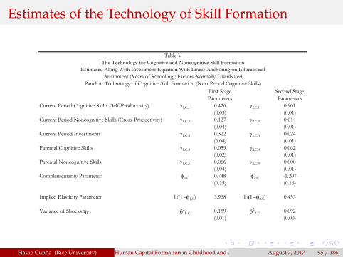
Estimates of the Technology of Skill Formation
First Stage Parameters
Second Stage Parameters
Current Period Cognitive Skills (Self-Productivity) g1,C,1 0.426 g2,C,1 0.901(0.03) (0.01)
Current Period Noncognitive Skills (Cross-Productivity) g1,C,2 0.127 g2,C,2 0.014(0.04) (0.01)
Current Period Investments g1,C,3 0.322 g2,C,3 0.024(0.04) (0.01)
Parental Cognitive Skills g1,C,4 0.059 g2,C,4 0.062(0.02) (0.01)
Parental Noncognitive Skills g1,C,5 0.066 g2,C,5 0.000(0.04) (0.01)
Complementarity Parameter f1,C 0.748 f2,C -1.207(0.25) (0.16)
Implied Elasticity Parameter 1/(1-f1,C) 3.968 1/(1-f2,C) 0.453Variance of Shocks hC,t d21,C 0.159 d22,C 0.092
(0.01) (0.00)
First Stage Parameters
Second Stage Parameters
Current Period Cognitive Skills (Cross-Productivity) g1,N,1 0.000 g2,N,1 0.000(0.02) (0.01)
Current Period Noncognitive Skills (Self-Productivity) g1,N,2 0.712 g2,N,2 0.868(0.03) (0.01)
Current Period Investments g1,N,3 0.195 g2,N,3 0.121(0.03) (0.03)
Parental Cognitive Skills g1,N,4 0.000 g2,N,4 0.000(0.01) (0.01)
Parental Noncognitive Skills g1,N,5 0.093 g2,N,5 0.011(0.03) (0.02)
Complementarity Parameter f1,N 0.017 f2,N -0.323(0.27) (0.21)
Elasticity Parameter 1/(1-f1,N) 1.017 1/(1-f2,N) 0.756Variance of Shocks hN,t d21,N 0.170 d22,N 0.104
(0.01) (0.00)Note: Standard errors in parenthesis.
Panel B: Technology of Noncognitive Skill Formation (Next Period Noncognitive Skills)
Table VEstimated Along With Investment Equation With Linear Anchoring on Educational
Panel A: Technology of Cognitive Skill Formation (Next Period Cognitive Skills)
The Technology for Cognitive and Noncognitive Skill FormationAttainment (Years of Schooling); Factors Normally Distributed
Flávio Cunha (Rice University) Human Capital Formation in Childhood and Adolescence August 7, 2017 95 / 186

Estimates of the Technology of Skill Formation
First Stage Parameters
Second Stage Parameters
Current Period Cognitive Skills (Self-Productivity) 1,C,1 0.426 2,C,1 0.901(0.03) (0.01)
Current Period Noncognitive Skills (Cross-Productivity) 1,C,2 0.127 2,C,2 0.014(0.04) (0.01)
Current Period Investments 1,C,3 0.322 2,C,3 0.024(0.04) (0.01)
Parental Cognitive Skills 1,C,4 0.059 2,C,4 0.062(0.02) (0.01)
Parental Noncognitive Skills 1,C,5 0.066 2,C,5 0.000(0.04) (0.01)
Complementarity Parameter 1,C 0.748 2,C -1.207(0.25) (0.16)
Implied Elasticity Parameter 1,C) 3.968 2,C) 0.453
Variance of Shocks C,t C 0.159 C 0.092(0.01) (0.00)
First Stage Parameters
Second Stage Parameters
Current Period Cognitive Skills (Cross-Productivity) 1,N,1 0.000 2,N,1 0.000(0.02) (0.01)
Current Period Noncognitive Skills (Self-Productivity) 1,N,2 0.712 2,N,2 0.868(0.03) (0.01)
Current Period Investments 1,N,3 0.195 2,N,3 0.121(0.03) (0.03)
Parental Cognitive Skills 1,N,4 0.000 2,N,4 0.000(0.01) (0.01)
Parental Noncognitive Skills 1,N,5 0.093 2,N,5 0.011(0.03) (0.02)
Complementarity Parameter 1,N 0.017 2,N -0.323(0.27) (0.21)
Elasticity Parameter 1,N) 1.017 2,N) 0.756
Variance of Shocks N,t N 0.170 N 0.104(0.01) (0.00)
Note: Standard errors in parenthesis.
Panel B: Technology of Noncognitive Skill Formation (Next Period Noncognitive Skills)
Table V
Estimated Along With Investment Equation With Linear Anchoring on Educational
Panel A: Technology of Cognitive Skill Formation (Next Period Cognitive Skills)
The Technology for Cognitive and Noncognitive Skill Formation
Attainment (Years of Schooling); Factors Normally Distributed
Flávio Cunha (Rice University) Human Capital Formation in Childhood and Adolescence August 7, 2017 96 / 186

Interpretation of Findings: Maximizing AverageEducation
Suppose that H children are born, h = 1, ...,H .These children represent draws from the distribution of initialconditions F (θc,1,h, θn,1,h, θc,p, θn,p,π).We want to allocate finite resources B across these children forearly and late investments.Formally:
S∗ = max1
H
[H
∑h=1
S(θc,3, θn,3,πh)
]subject to the technologies for the formation of cognitive andnoncognitive skills as well as:
∑H
h=1(x1,h + x2,h) = B
Flávio Cunha (Rice University) Human Capital Formation in Childhood and Adolescence August 7, 2017 97 / 186

Interpretation of Findings: Minimizing Average Crime
Another possibility is to minimize aggregate crime (average crimeper individual).This will lead to different optimal ratios as crime is more sensitiveto changes in noncognitive skills.Relative to cognitive skills, noncognitive skills are more malleableat later ages.
Flávio Cunha (Rice University) Human Capital Formation in Childhood and Adolescence August 7, 2017 98 / 186

COGNITIVE AND NONCOGNITIVE SKILL FORMATION 925
FIGURE 5.—Ratio of early to late investments by maternal cognitive and noncognitive skillsmaximizing aggregate education (left) and minimizing aggregate crime (right) (other endow-ments held at mean levels).
FIGURE 6.—Densities of ratio of early to late investments maximizing aggregate educationversus minimizing aggregate crime.

Books Ages 3‐4Mom Reads to Child Ages 3‐4Eats with Mom/Dad Ages 3‐4
Magazines Ages 3‐4CD player Ages 3‐4Outings Ages 5‐6Books Ages 5‐6
Mom Reads to Child Ages 5‐6Eats with Mom/Dad Ages 5‐6
Magazines Ages 5‐6
Figure 5AShare of Residual Variance in Measurements of Investments
Due to the Variance of Investment Factor (Signal) and Due to the Variance of Measurement Error (Noise)
0% 10% 20% 30% 40% 50% 60% 70% 80% 90% 100%
Outings BirthBooks Birth
Mom Reads to Child BirthSoft Toys Birth
Push/Pull Toys BirthEats with Mom/Dad Birth
Mom Calls from Work BirthOutings Ages 1‐2Books Ages 1‐2
Mom Reads to Child Ages 1‐2Soft Toys Ages 1‐2
Push/Pull Toys Ages 1‐2Eats with Mom/Dad Ages 1‐2Mom Calls from Work Ages …
Outings Ages 3‐4
Percentage
Signal Error

Special Lessons Ages 7‐8Musical Shows Ages 7‐8
Family Gatherings Ages 7‐8Praises Ages 7‐8
Encouragement Ages 7‐8Books Ages 9‐10
Mom Reads to Child Ages 9‐10Eats with Mom/Dad Ages 9‐10
Museum Ages 9‐10Musical Instruments Ages 9‐10
Figure 5BShare of Residual Variance in Measurements of Investments
Due to the Variance of Investment Factor (Signal) and Due to the Variance of Measurement Error (Noise)
0% 10% 20% 30% 40% 50% 60% 70% 80% 90% 100%
CD player Ages 5‐6Museum Ages 5‐6
Musical Instruments Ages 5‐6Daily Newspapers Ages 5‐6
Special Lessons Ages 5‐6Musical Shows Ages 5‐6
Family Gatherings Ages 5‐6Praises Ages 5‐6
Encouragement Ages 5‐6Books Ages 7‐8
Mom Reads to Child Ages 7‐8Eats with Mom/Dad Ages 7‐8
Museum Ages 7‐8Musical Instruments Ages 7‐8
Daily Newspapers Ages 7‐8
Percentage
Signal Error

E t A 11 12Books Ages 13‐14
Eats with Mom/Dad Ages …Museum Ages 13‐14
Musical Instruments Ages …Daily Newspapers Ages 13‐14
Special Lessons Ages 13‐14Musical Shows Ages 13‐14
Family Gatherings Ages 13‐14Praises Ages 13‐14
Encouragement Ages 13‐14
Figure 5CShare of Residual Variance in Measurements of Investments
Due to the Variance of Investment Factor (Signal) and Due to the Variance of Measurement Error (Noise)
0% 10% 20% 30% 40% 50% 60% 70% 80% 90% 100%
Daily Newspapers Ages 9‐10Special Lessons Ages 9‐10Musical Shows Ages 9‐10
Family Gatherings Ages 9‐10Praises Ages 9‐10
Encouragement Ages 9‐10Books Ages 11‐12
Eats with Mom/Dad Ages …Museum Ages 11‐12
Musical Instruments Ages …Daily Newspapers Ages 11‐12
Special Lessons Ages 11‐12Musical Shows Ages 11‐12
Family Gatherings Ages 11‐12Praises Ages 11‐12
Encouragement Ages 11‐12
Percentage
Signal Error

Home Observation for the Measurement of theEnvironment
Created by Bettye Caldwell and Robert Bradley in late 1960s, early1970s (first published in 1980s)Evaluates a child’s home environment as well as parent-childinteraction.Administered by trained professional at the child’s home withboth child and primary caregiver present.Semi-structured interview and observation period: 45-60 minutes.
Flávio Cunha (Rice University) Human Capital Formation in Childhood and Adolescence August 7, 2017 103 / 186

HOME: Strenghts and Weakenesses
Strenghts
Easy to administer and score.Reliability and validity.Easy to adapt for specific purposes.Provides objective information on home, child, and parent-childinteraction.
Weakenesses:
Training of administrators to follow standardized measurement.Only Yes/No questions.Score: Simple summation gives “too much” weight to items that donot vary a lot across households.
Flávio Cunha (Rice University) Human Capital Formation in Childhood and Adolescence August 7, 2017 104 / 186

HOME: IRT Analysis
Let θi denote the latent quality of the environment experienced bychild i .Let d∗i ,j = aj (θi − bj ) + εi ,j and define di ,j = 0 if d∗i ,j ≤ 0 anddi ,j = 1, otherwise.Assume εi ,j has logistic distribution and let θi be normallydistributed with mean zero and variance σ2.Parameter aj is item discrimination while bj is item difficulty.
Flávio Cunha (Rice University) Human Capital Formation in Childhood and Adolescence August 7, 2017 105 / 186

Interpretation of IRT Parameters
Section 5: The two-parameter logistic (2PL) model 25
tradition; the same is true of the symbol a since slopes are usually denoted with b instatistics.
We saw on Figure 6 that the IRF in a 1PL model run parallel to each other andnever cross; different difficulty parameters solely shift the curve to the left or to theright while its shape remains unchanged.
Pi(θ, bi, ai)
−4 −3 −2 −1 0 1 2 3 40
0.5
1.0
θ
Figure 13: The item response functions ofthree 2PL items
A very different picture is observed onFigure 13. Two of the items have the samedifficulty of −1.0. As in the 1PL, the difficultyis found at the ability level that yields a proba-bility of 0.5. However, the blue curve is muchsteeper than the black one. This is becausethe item with the blue curve has a higher dis-crimination parameter than the item with theblack curve. The discrimination parametersai are sometimes called slope parameters, justlike the item difficulties are a.k.a. location pa-rameters. The slope of the 2PL item response
function at b is equal to a/4.What about the green curve? It has the same slope as the black one but it is
shifted to the right — hence the item with the green curve has the same discrimina-
Flávio Cunha (Rice University) Human Capital Formation in Childhood and Adolescence August 7, 2017 106 / 186

Properties of an Informative IRT Scale
Flávio Cunha (Rice University) Human Capital Formation in Childhood and Adolescence August 7, 2017 107 / 186

Properties of an Informative IRT Scale: IIF
Flávio Cunha (Rice University) Human Capital Formation in Childhood and Adolescence August 7, 2017 108 / 186

Properties of an Informative IRT Scale: TCC
Flávio Cunha (Rice University) Human Capital Formation in Childhood and Adolescence August 7, 2017 109 / 186

Properties of an Informative IRT Scale: TIF
Flávio Cunha (Rice University) Human Capital Formation in Childhood and Adolescence August 7, 2017 110 / 186

HOME: IRT Analysis
In few words, an informative scale (as presented in the last fourgraphs) would have items that have good discriminatory poweras well as variability in difficulty.This combination allows us to identify, with a lot of precision,households that have low, medium, and high qualityenvironments.Unfortunately, the HOME Scale does not have this property.As I will show below, that are “too many” easy items and “toofew” medium and difficult items.For this reason, the HOME Scale will be able to separate very lowquality home environments from okay ones, but it will not havepower to separate okay from great home environments.
Flávio Cunha (Rice University) Human Capital Formation in Childhood and Adolescence August 7, 2017 111 / 186

IRT Properties of Full Scale HOME
Flávio Cunha (Rice University) Human Capital Formation in Childhood and Adolescence August 7, 2017 112 / 186

IRT Properties of Full Scale HOME
Flávio Cunha (Rice University) Human Capital Formation in Childhood and Adolescence August 7, 2017 113 / 186

IRT Properties of Full Scale HOME
Flávio Cunha (Rice University) Human Capital Formation in Childhood and Adolescence August 7, 2017 114 / 186

IRT Properties of Full Scale HOME
Flávio Cunha (Rice University) Human Capital Formation in Childhood and Adolescence August 7, 2017 115 / 186

Why does the IRT Properties of the HOME Matter?
It probably affects the estimation of the technology of skillformation.Why? Medium and high quality environments are difficult toseparate.It is possible that differences between medium and high qualityenvironments are more (or less) important for child developmentthan differences between medium and low quality environments.Either case may lead to biases in the estimation of the technologyof skill formation.
Flávio Cunha (Rice University) Human Capital Formation in Childhood and Adolescence August 7, 2017 116 / 186

Monte Carlo Exercise
Let h1 denote human capital, θ denote investments, and ζ denoteuncorrelated shocks. Consider the simple technology of skillformation:
h1 = 1.0+ 0.5θ − 0.25θ2 + ζ (1)
To obtain an idea about potential problems of using the HOME asa measure of investment to be used in the estimation of (1):
Generate a HOME Scale with desirable IRT properties as the“desired” HOME Scale;Generate a HOME Scale that has “flawed” IRT properties as the“actual” HOME Scale;Estimate θdesired from “desired” HOME Scale and θflawed from“actual” HOME Scale;Regress h1 on quadratic function of θdesired and compare estimatedwith true coefficients;Regress h1 on quadratic function of θflawed and compare estimatedwith true coefficients.
Flávio Cunha (Rice University) Human Capital Formation in Childhood and Adolescence August 7, 2017 117 / 186

Flávio Cunha (Rice University) Human Capital Formation in Childhood and Adolescence August 7, 2017 118 / 186

Measuring Quality and Quantity of Time: LENA Pro
Flávio Cunha (Rice University) Human Capital Formation in Childhood and Adolescence August 7, 2017 119 / 186

Measuring Quality and Quantity of Time: LENA Pro
Flávio Cunha (Rice University) Human Capital Formation in Childhood and Adolescence August 7, 2017 120 / 186

Reliability: Adult Word Counts
Flávio Cunha (Rice University) Human Capital Formation in Childhood and Adolescence August 7, 2017 121 / 186

Measuring Quality and Quantity of Time: LENA Pro
Flávio Cunha (Rice University) Human Capital Formation in Childhood and Adolescence August 7, 2017 122 / 186

Measuring Quantity of Time: Meaningful TimePhiladelphia Human Development Study
Flávio Cunha (Rice University) Human Capital Formation in Childhood and Adolescence August 7, 2017 123 / 186

Measuring Quality of Time: Conversation TurnCountsPhiladelphia Human Development Study
Flávio Cunha (Rice University) Human Capital Formation in Childhood and Adolescence August 7, 2017 124 / 186

Measuring Quality and Quantity of Time: LENA ProPhiladelphia Human Development Study
Flávio Cunha (Rice University) Human Capital Formation in Childhood and Adolescence August 7, 2017 125 / 186

Count Data
This dependence between mean and variance (in hours when themean is high, the variance is also high) is typical in count data.One may think of taking the natural log of conversation turncounts and proceed with OLS-type analysis.Not a good idea with count data:
There are many zeros; taking the logs will eliminate the zeros fromthe analysis, which means it reduces cases of poor languageenvironment.We want to identify households in terms of expected number ofcounts, not the expected log of number of counts (nonlineartransformation).
Flávio Cunha (Rice University) Human Capital Formation in Childhood and Adolescence August 7, 2017 126 / 186

Analysis of LENA Conversation Turn Counts Data
Let Yi ,j denote the jth observation on conversation turn countsbetween an adult and child i .Because these are counts, we model each observation as a Poissonrandom variable with parameter εi λi ,j where εi is a random effectterm and λi ,j is such that:
lnλi ,j = Xi ,j δj + ln si ,j (2)
Vector Xi ,j contains variables that describe the context ofmeasurement and si ,j is “exposure” (i.e., number of seconds thatthe LENA device was on during the jth measurement).
Flávio Cunha (Rice University) Human Capital Formation in Childhood and Adolescence August 7, 2017 127 / 186

Flávio Cunha (Rice University) Human Capital Formation in Childhood and Adolescence August 7, 2017 128 / 186

Flávio Cunha (Rice University) Human Capital Formation in Childhood and Adolescence August 7, 2017 129 / 186

Flávio Cunha (Rice University) Human Capital Formation in Childhood and Adolescence August 7, 2017 130 / 186

Analysis of LENA Conversation Turn Counts Data
Conditional on εi , the probability of observing a count equal to:
Pr (yi ,j | εi ) =(εi λi ,j )
yi ,j
yi ,j !e−εi λi ,j
where Pr (yi ,j | εi ) = Pr (Yi ,j = yi ,j | εi ) is the probability that thecount of variable Yi ,j is equal to yi ,j conditional on εi .Assume that, conditional on εi , the events are independent. Thus:
Pr (yi ,1, ..., yi ,J | εi ) =
{[J
∏j=1
(λi ,j )yi ,j
yi ,j !
]ε
∑Jj=1 yi ,j
i e−εi ∑Jj=1 λi ,j
}(3)
Because we don’t observe the random effect εi , we need tointegrate it out.We assume that εi has gamma distribution with mean one andvariance 1
α
Flávio Cunha (Rice University) Human Capital Formation in Childhood and Adolescence August 7, 2017 131 / 186

Flávio Cunha (Rice University) Human Capital Formation in Childhood and Adolescence August 7, 2017 132 / 186

Analysis of LENA Conversation Turn Counts Data
Let Mi ,j denote the share of meaningful time of adult-childinteraction in jth observation.Because these are proportion data, we model each observation asthe following logistic regression:
ln
{Mi ,j
1−Mi ,j
}= Xi ,j ρj + µi + νi ,j
where µi is a random effect with mean zero and variance σ2µ .
We are interested in estimating the unobserved heterogeneitycaptured by µi across families.
Flávio Cunha (Rice University) Human Capital Formation in Childhood and Adolescence August 7, 2017 133 / 186

Flávio Cunha (Rice University) Human Capital Formation in Childhood and Adolescence August 7, 2017 134 / 186

Flávio Cunha (Rice University) Human Capital Formation in Childhood and Adolescence August 7, 2017 135 / 186

Flávio Cunha (Rice University) Human Capital Formation in Childhood and Adolescence August 7, 2017 136 / 186

Introducing Heterogeneity in Beliefs
0 5 10 15 20 25 30 35 400
20
40
60
80
100
120
Child Development
Oth
er E
xpen
ditu
res
FigureChoice Set and Preferences
Red: Mother underestimates returnsBlue: Mother has unbiased returns
Flávio Cunha (Rice University) Human Capital Formation in Childhood and Adolescence August 7, 2017 137 / 186

Why Heterogeneity in Beliefs?
Language acquisition: Hart and Risley (1995); Rowe (2008).Time spent in activities that are appropriate for the child’s age(Kalil et al, 2012).Home visitation programs on parenting:
Nurse-Family Partnership (Olds et al, 2012).Jamaican Nutrition Supplementation and Cognitive StimulationProgram (Gertler et al, 2014; Attanasio et al, 2014).HIPPY Program (Baker et al, 2002).Parent as Teachers (PAT, Wagner et al, 1998)Play and Learning Strategies (PALS, Landry et al, 1996).Thirty Million Words Program (Suskind and Lefler, 2013).Many others (Healthy Families, Healthy Start, CHIP of Virginia,MOM of Philadelphia, etc.)
Flávio Cunha (Rice University) Human Capital Formation in Childhood and Adolescence August 7, 2017 138 / 186

Research Questions
My current research aims to answer the following questions:
Can we measure parental beliefs about the technology of skillformation?If so:
How do parental beliefs compare with objective estimates of thetechnology of skill formation?Is there heterogeneity in parental beliefs?
If so, does the heterogeneity in beliefs predict heterogeneity ininvestments?If so, can we change parental investments by affecting parentalbeliefs?
Flávio Cunha (Rice University) Human Capital Formation in Childhood and Adolescence August 7, 2017 139 / 186

Model: The technology of skill formation
The technology of skill formation is:
ln hi ,1 = ψ0 + ψ1 ln h0,i + ψ2 ln xi + ψ3 ln h0,i lnXi + νi
Flávio Cunha (Rice University) Human Capital Formation in Childhood and Adolescence August 7, 2017 140 / 186

Model: The mother’s information set
Let Ψi denote the mother’s information set.Let E (ψj | h0,i , xi ,Ψi ) = µi ,j and assume that E (νi |Ψi ) = 0.From the point of view of the mother:
E ( ln hi ,1| h0,i , xi ,Ψi ) = µi ,0 + µi ,1 ln h0,i + µi ,2 ln xi + µi ,3 ln h0,i ln xi
Flávio Cunha (Rice University) Human Capital Formation in Childhood and Adolescence August 7, 2017 141 / 186

Model: Preferences and budget constraint
Consider a simple static model. Parent’s utility is:
u (ci , hi ,1; αi ,1, αi ,2) = ln ci + αi ,1 ln hi ,1 + αi ,2 ln xi
Budget constraint is:ci + pxi = yi .
Flávio Cunha (Rice University) Human Capital Formation in Childhood and Adolescence August 7, 2017 142 / 186

Model
The problem of the mother is to maximize expected utility subjectto the mother’s information set, the budget constraint, and thetechnology of skill formation.The solution is
xi =
[αi ,1 (µi ,2 + µi ,3 ln h0,i ) + αi ,2
1+ αi ,1 (µi ,2 + µi ,3 ln h0,i ) + αi ,2
]yi
p
Clearly, we cannot separately identify αi from µi ,γ if we onlyobserve xi , yi , and p.
Flávio Cunha (Rice University) Human Capital Formation in Childhood and Adolescence August 7, 2017 143 / 186

Identification
Elicit maternal beliefs.Elicit maternal preferences.Estimate the technology of skill formation.
Flávio Cunha (Rice University) Human Capital Formation in Childhood and Adolescence August 7, 2017 144 / 186

Eliciting beliefs: Steps
Measure actual child development: MSD and Item ResponseTheory (IRT).Develop the survey instrument to elicit beliefs E [ ln hi ,1| h0, x ,ψi ]:
Reword MSD items.Create hypothetical scenarios of h0 and x .
Estimate beliefs from answers allowing for error in responses.
Flávio Cunha (Rice University) Human Capital Formation in Childhood and Adolescence August 7, 2017 145 / 186


Eliciting beliefs: Item response theory
Let d∗i ,j = b0,j + b1,j
(ln ai +
b2,jb1,j
θi
)+ ηi ,j
We observe di ,j = 1 if d∗i ,j ≥ 0 and di ,j = 0, otherwise.
Measure of (log of) human capital: ln hi = ln ai +b2,jb1,j
θi .
In this sense, θi is deviation from typical development for age.
Flávio Cunha (Rice University) Human Capital Formation in Childhood and Adolescence August 7, 2017 147 / 186

0.2
5.5
.75
1P
roba
bilit
y
0 4 8 12 16 20 24 28 32 36 40 44 48Child Age (Months)
Speak partial sentence, data Speak partial sentence, predicted
Probability as a Function of Child's AgeFigure 4

Eliciting beliefs: Changing wording of the MSDInstrument
In order to measure E [ ln hi ,1| h0, x ,ψi ], we take the tasks from theMSD Scale, but instead of asking: “Has your child ever spoken apartial sentence with three words or more?”, we ask:Method 1: How likely is it that a baby will speak a partialsentence with three words or more by age 24 months?Method 2: What is the youngest and oldest age a baby learns tospeak a partial sentence with three words or more?
Flávio Cunha (Rice University) Human Capital Formation in Childhood and Adolescence August 7, 2017 149 / 186

Eliciting beliefs: Scenarios of human capital andinvestments
We consider four scenarios:
Scenario 1: Child is healthy at birth (e.g., normal gestation, birthweight, and birth length) and investment is high (e.g., six hours perday).Scenario 2: Child is healthy at birth and investment is low (e.g., twohours per day).Scenario 3: Child is not healthy at birth (e.g., premature, low birthweight, and small at birth) and investment is high.Scenario 4: Child is not healthy at birth and investment is low.
Scenarios are described to survey respondents through a video.
Flávio Cunha (Rice University) Human Capital Formation in Childhood and Adolescence August 7, 2017 150 / 186

Method 1: Transforming probabilities into meanbeliefs
Method 1: How likely is it that a baby will speak a partialsentence with three words or more by age 24 months?Let’s say that when investment is high – that is, when x = x – themother states that there is a 75% chance that the child will learnhow to speak a partial sentence with three words or more.And when investment is low– that is, when x = x – the motherstates that there is a 25% chance that the child will learn how tospeak a partial sentence with three words or more.We convert this probability statement into an age-equivalentstatement using the NHANES data.
Flávio Cunha (Rice University) Human Capital Formation in Childhood and Adolescence August 7, 2017 151 / 186

0.2
5.5
.75
1P
roba
bilit
y
0 4 8 12 16 20 24 28 32 36 40 44 48Child Age (Months)
Speak partial sentence, data Speak partial sentence, predicted
Probability as a Function of Child's AgeFigure 4

Method 2: Transforming age ranges into probabilies
Method 2: What is the youngest and oldest age a baby learns tospeak a partial sentence with three words or more?Let’s say that when investment is high, so that x = x , the motherstates that the youngest and oldest ages a baby will learn how tospeak a sentence with three words or more are, respectively, 18and 28 months.And when investment is low, so that x = x , the mother states thatthe ages are 20 and 30 months.We need to transform the age ranges into probabilities. We use theage ranges to estimate a mother-specific IRT model.
Flávio Cunha (Rice University) Human Capital Formation in Childhood and Adolescence August 7, 2017 153 / 186

0.2
5.5
.75
1P
roba
bilit
y
0 4 8 12 16 20 24 28 32 36 40 44 48Age (in months)
High investment
Transforming age range into probabilityFigure 3

0.2
5.5
.75
1P
roba
bilit
y
0 4 8 12 16 20 24 28 32 36 40 44 48Age (in months)
Logistic prediction, high High investment
Transforming age range into probabilityFigure 3

0.2
5.5
.75
1P
roba
bilit
y
0 4 8 12 16 20 24 28 32 36 40 44 48Age (in months)
Logistic prediction, high High investment
Transforming age range into probabilityFigure 3

0.2
5.5
.75
1P
roba
bilit
y
0 4 8 12 16 20 24 28 32 36 40 44 48Age (in months)
Logistic prediction, high High investment
Logistic prediction, low Low investment
Transforming age range into probabilityFigure 3

0.2
5.5
.75
1P
roba
bilit
y
0 4 8 12 16 20 24 28 32 36 40 44 48Age (in months)
Logistic prediction, high High investment
Logistic prediction, low Low investment
Transforming age range into probabilityFigure 3

Method 2: Transforming probabilities into meanbeliefs
Method 2: Given scenario for h0 and x , how likely is it that ababy will speak a partial sentence with three words or more byage 24 months?Given maternal supplied age range and the logistic assumption,we conclude that when x = x , the mother believes that there is a75% chance that the child will learn how to speak a partialsentence with three words or more.Analogously, when x = x , the mother believes that there is a 25%chance that the child will learn how to speak a partial sentencewith three words or more.We convert this probability statement into an age-equivalentstatement using the NHANES data.
Flávio Cunha (Rice University) Human Capital Formation in Childhood and Adolescence August 7, 2017 159 / 186

0.2
5.5
.75
1P
rob
ab
ility
0 4 8 12 16 20 24 28 32 36 40 44 48Child Age (in months)
High x Low x
Speak partial sentence - MKIDSAge range to probability
0.2
5.5
.75
1P
rob
ab
ility
0 4 8 12 16 20 24 28 32 36 40 44 48Child Age (Months)
Data Predicted
Speak partial sentence - NHANESProbability to expected development
Expected development for two levels of investments (x)Figure 3

Recovering mean beliefs: Measurement error model
Let ln qLi ,j ,k denote an error-ridden measure of E [ ln hi ,1| h0,k , xk ,ψi ]
generated by “how likely” questions:
ln qLi ,j ,k = E [ ln hi ,1| h0,k , xk ,ψi ] + εL
i ,j ,k .
Let ln qAi ,j ,k denote an error-ridden measure of E [ ln hi ,1| h0,k , xk ,ψi ]
generated by “age range” questions:
ln qAi ,j ,k = E [ ln hi ,1| h0,k , xk ,ψi ] + εA
i ,j ,k .
For each scenario, we have multiple measures of the sameunderlying latent variable.
Flávio Cunha (Rice University) Human Capital Formation in Childhood and Adolescence August 7, 2017 161 / 186

Recovering mean beliefs:
Use technology of skill formation, and the mother’s informationset, to obtain:
ln qLi ,j ,k = µi ,0 + µi ,1 ln h0,k + µi ,2 ln xk + µi ,3 ln h0,k ln xk + εL
i ,j ,k
ln qAi ,j ,k = µi ,0 + µi ,1 ln h0,k + µi ,2 ln xk + µi ,3 ln h0,k ln xk + εA
i ,j ,k ..
We have a factor model where:
µi = (µi ,0, µi ,1, µi ,2, µi ,3) are the latent factors;λk = (1, h0,k , ln xk , ln h0,k ln xk ) are the factor loadings;
εi ,j,k =(
εLi ,j,k , εA
i ,j,k
)are the uniquenesses.
Flávio Cunha (Rice University) Human Capital Formation in Childhood and Adolescence August 7, 2017 162 / 186

Eliciting beliefs: Intuitive explanation
Let E [ ln hi ,1| h0, h,Ψi ] denote maternal expectation of childdevelopment at age 24 months conditional on the child’s intiallevel of human capital, investments, and the mother’s informationset.Assume, for now, technology is Cobb-Douglas.Suppose we measure E [ ln hi ,1| h0, x ,Ψi ] at two different levels ofinvestments:
E [ ln hi ,1| h0, x ,Ψi ] = µi ,0 + µi ,1 ln h0 + µi ,2 ln x
E [ ln hi ,1| h0, x ,Ψi ] = µi ,0 + µi ,1 ln h0 + µi ,2 ln x
Subtracting and re-organizing terms:
µi ,2 =E [ ln hi ,1| h0, x ,Ψi ]− E [ ln hi ,1| h0, x ,Ψi ]
ln x − ln x
Flávio Cunha (Rice University) Human Capital Formation in Childhood and Adolescence August 7, 2017 163 / 186

Important issue
We could use only one MSD item to elicit beliefs.But, if we use more items, we can relax assumptions aboutmeasurement error.And, we can check for consistency in answers.
Flávio Cunha (Rice University) Human Capital Formation in Childhood and Adolescence August 7, 2017 164 / 186

Speaks partial sentence
Knows own age and sex
0.2
5.5
.75
1
0 4 8 12 16 20 24 28 32 36 40 44 48Age (in months)
Age range into probabilitySpeaks partial sentence
Knows own age and sex
0.2
5.5
.75
1
0 4 8 12 16 20 24 28 32 36 40 44 48Child Age (Months)
Probability into expected development
Speaks partial sentence
Knows own age and sex
0.2
5.5
.75
1
0 4 8 12 16 20 24 28 32 36 40 44 48Age (in months)
Speaks partial sentence
Knows own age and sex
0.2
5.5
.75
1
0 4 8 12 16 20 24 28 32 36 40 44 48Child Age (Months)
Comparing answers across scenariosFigure 5

Estimation of Preferences
The investment policy function is:
xi =
[αi ,1 (µi ,2 + µi ,3 ln h0,i ) + αi ,2
1+ αi ,1 (µi ,2 + µi ,3 ln h0,i ) + αi ,2
]yi
p
where αi ,1 and αi ,2 captures heterogeneity in preferences.The usual procedure is to work with observed investment data.We are in the field collecting these investment data.
Flávio Cunha (Rice University) Human Capital Formation in Childhood and Adolescence August 7, 2017 166 / 186

Estimation of Preferences
Today, we elicit the preference parameters by stated-choice data(as it is commonly applied in Marketing).We tell the respondent to assume that the child’s initial level ofhuman capital is high.Then, we create nine hypothetical scenarios of monthly incomeand prices:
Parental preferences
I Our approach is to elicit the preference parameter bystated-choice data.
I We first tell the respondent to assume that the child’s healthcondition at birth is “high”.
I Then, we create nine hypothetical scenarios of monthlyincome and prices:
Price
Income
$30 $45 $60$1500 Scenario 1 Scenario 2 Scenario 3$2000 Scenario 4 Scenario 5 Scenario 6$2500 Scenario 7 Scenario 8 Scenario 9
Flávio Cunha (Rice University) Human Capital Formation in Childhood and Adolescence August 7, 2017 167 / 186

Estimation of Preferences
In order to link investment to time, we prepared a three-minutevideo in which we explain to the respondent that the more timethat the mother interacts with the child, the more money she hasto spend every month buying educational goods such as childbooks and educational toys.Our goal is to pass on to the respondent the idea that investmentis costly.Respondents are not familiar with the concept of “opportunitycost.”
Flávio Cunha (Rice University) Human Capital Formation in Childhood and Adolescence August 7, 2017 168 / 186

Estimation of Preferences
For each combination of prices and income, we ask therespondents the following question: Suppose that your householdincome is $y per month and that for each hour per day that the motherspends interacting with the child she has to spend $p per month oneducational goods. Consider the following four options:The four options correspond to two, three, four, and five hours ofinvestments per day.Thus, if the respondent reports xi ,m,n hours of investment per daywhen price is pm and income is yn, then share of income allocatedto investments, sm,n is:
si ,m,n =pmxi ,m,n
yn
Flávio Cunha (Rice University) Human Capital Formation in Childhood and Adolescence August 7, 2017 169 / 186

Estimation of Preferences
Note that the ratio, ri ,m,n is:
ri ,m,n =si ,m,n
1− si ,m,n= αi ,1 (µi ,2 + µi ,3 ln h0,i ) + αi ,2 + ξi ,m,n
.The parameters αi ,1 and αi ,2 can be estimated as a simplerandom-effects model.
Flávio Cunha (Rice University) Human Capital Formation in Childhood and Adolescence August 7, 2017 170 / 186

Descriptive Information about Participants: MKIDSand PHDPilot Study: Maternal Knowledge of Infant Development Study (MKIDS)
777 participants, all African-American.MKIDS: 60% are primiparous; PHD: 100% are primiparous.80% are single (not cohabiting or married).80% are at most 25 years-old.Median household income is below the second decile of U.S.distribution.Low education sample: only 12% of respondents have a two-yearcollege degree or more.
Flávio Cunha (Rice University) Human Capital Formation in Childhood and Adolescence August 7, 2017 171 / 186

N % N % N %
20 6.2 0 0.0 20 2.6233 72.1 0 0.0 233 30.070 21.7 454 100.0 524 67.4
323 100.0 0 0.0 323 41.6323 100.0 454 100.0 777 100.0323 100.0 454 100.0 777 100.0323 100.0 454 100.0 777 100.0323 100.0 454 100.0 777 100.0323 100.0 0 0.0 323 41.6323 100.0 0 0.0 323 41.6323 100.0 0 0.0 323 41.6
158 48.9 454 100.0 612 78.842 13.0 0 0.0 42 5.491 28.2 0 0.0 91 11.732 9.9 0 0.0 32 4.1
Table 1Comparison of Datasets
TotalMKIDS PHD454 777Number of observations 323
Type of Elicitation MethodOnly probabilityOnly age ranges
158 48.9
Stated choice dataHypothetical scenarios for prices
of investment and income
Hypothetical scenariosBaseline
Alternative scenario #1Alternative scenario #2Alternative scenario #3
158 20.3
Both methodsMSD Items
Wearing wet pants bothers childSpeak partial sentenceSay first and last name
Count 3 objects correctlyKnow own age and sex
Says the names of 4 colorsCount out loud up to 10
Draw picture of man/woman
0 0.0

Rank Item Description Obs. 1 2 3 4 Obs. 1 2 3 4
0.78 0.55 0.70 0.51 0.64 0.55 0.50 0.43(0.24) (0.27) (0.27) (0.26) (0.33) (0.36) (0.36) (0.37)
0.81 0.63 0.61 0.45 0.60 0.44 0.42 0.31(0.18) (0.22) (0.20) (0.20) (0.36) (0.38) (0.38) (0.36)
0.84 0.67 0.62 0.47 0.41 0.32 0.26 0.19(0.18) (0.22) (0.20) (0.20) (0.38) (0.36) (0.33) (0.30)
0.83 0.66 0.62 0.47 0.33 0.26 0.23 0.17(0.19) (0.23) (0.21) (0.21) (0.36) (0.33) (0.31) (0.29)
0.80 0.64 0.60 0.46 0.31 0.24 0.22 0.17(0.20) (0.22) (0.21) (0.21) (0.36) (0.33) (0.31) (0.29)
0.81 0.59 0.74 0.56 0.26 0.22 0.19 0.16(0.23) (0.28) (0.22) (0.27) (0.31) (0.29) (0.28) (0.26)
0.80 0.58 0.75 0.53 0.24 0.20 0.19 0.16(0.20) (0.27) (0.19) (0.27) (0.30) (0.28) (0.28) (0.27)
0.71 0.51 0.67 0.48 0.15 0.15 0.14 0.13(0.25) (0.28) (0.21) (0.26) (0.26) (0.26) (0.26) (0.25)
7
Note: Standard errors in parenthesis.
8
Child says the names of at least 4 colors
303
3030.02 90
90
5
6
1
2
3
4
Table 2Basic Features of Raw Data
MSD Items ranked in ascending order of difficulty
0.07 90
303
757
757
757
757
303
0.39 544
0.31 544
0.20
Chils lets someone know that wearing wet pants bothers him/her?
Child speaks a partial sentence of 3 words or more
Child says first and last name together without someone's help
Child draws a picture of a man/woman, 2 parts besides head
0.99
Child counts 3 objects correctly?
Child counts out loud up to 10?
Child knows own age and sex
90
0.72 544
0.26 544
ScenariosScenariosProbability Age ranges
NHANES

Beliefs about the technology of skill formation
25th percentile Median 75th
percentile Mean Variance
-0.015 0.101 0.236 0.115 0.035(0.009) (0.008) (0.009) (0.007) (0.002)0.077 0.296 0.554 0.365 0.204
(0.011) (0.016) (0.022) (0.016) (0.026)0.065 0.166 0.285 0.192 0.046
(0.006) (0.007) (0.010) (0.008) (0.005)-0.008 0.094 0.335 0.190 0.320(0.007) (0.010) (0.024) (0.020) (0.051)
Note: Standard errors in parenthesis.
Table 3Maternal Beliefs about the Technology of Skill Formation
,0
,1
,3
,2
Flávio Cunha (Rice University) Human Capital Formation in Childhood and Adolescence August 7, 2017 174 / 186

Sensitivity analysis
F Test,0 ,1 ,2 ,3 (p-value)0.018 0.147 0.112 0.070 -
(0.017) (0.043) (0.022) (0.062) -0.067 -0.027 -0.032 -0.081 1.080
(0.037) (0.094) (0.048) (0.136) (0.364)0.280 0.469 0.175 0.424 33.910
(0.028) (0.071) (0.037) (0.103) (0.000)0.206 0.027 0.051 0.091 6.750
(0.041) (0.104) (0.054) (0.152) (0.000)
Table 4Alternative Definition of Scenarios and Maternal Beliefs
Note: Standard errors in parenthesis, except in the F-test column where we report p-values.
Dependent variablesRegressors
Intercept (baseline)
Dummy for alternative scenario #1
Dummy for alternative scenario #3
Dummy for alternative scenario #2
Flávio Cunha (Rice University) Human Capital Formation in Childhood and Adolescence August 7, 2017 175 / 186

3.2
3.4
3.6
3.8
44
.2
30 40 50 60Price
Income = $1500 Income = $2000
Income = $2500
Demand curves
3.2
3.4
3.6
3.8
44
.2
1500 2000 2500Income
Price = $30 Price = $45
Price = $45
Engel curves
Figure 9

Preferences
25th percentile Median 75th
percentile Mean Variance
0.0261 0.0312 0.0400 0.0313 0.0002(0.0004) (0.0002) (0.0007) (0.0004) (0.0000)0.0669 0.0777 0.0942 0.0795 0.0003(0.0005) (0.0008) (0.0007) (0.0005) (0.0000)
Note: Standard errors in parenthesis.
Table 5Maternal Beliefs about the Technology of Skill Formation
i,1
i,2
Flávio Cunha (Rice University) Human Capital Formation in Childhood and Adolescence August 7, 2017 177 / 186

Preferences
Median 75th percentile
% Change in investments
% Change in parameter Elasticity
1 1.70 1.73 1.6% 28.0% 5.8%2 1.70 2.01 18.3% 21.4% 85.2%,2 1.70 1.77 4.1% 72.0% 5.8%,3 1.70 1.70 0.2% 257.1% 0.1%,3 1.70 1.86 9.3% 257.1% 3.6%
Table 7Comparative Statics of Investments
This table shows the comparative statics of optimal investments in relation to preference and belief parameters. Each row shows what happens to investments as we move one parameter and fix the other parameters at the median value. In the last row, we replace the human capital at birth from the mean value to the value at the first percentile.
Flávio Cunha (Rice University) Human Capital Formation in Childhood and Adolescence August 7, 2017 178 / 186

Cases Factual investment
Counterfactual investment % Change Effect size
,2 = 0.267,3 = 0.000
,2 = 0.454,3 = 0.000
1.84 2.05 11.7% 26.9%
Table 8Maternal Beliefs and Technology
1.84 1.92 4.4% 10.3%

Beliefs and Investments: Anthropology
!Kung San in the Kalahari desert in Botswana and Namibia (e.g.,Lee, 1979) vs. Ache in Paraguay (see Kaplan and Dove, 1987; Hilland Hurtado, 1996).
Both groups believe that the development of motor skills bychildren depends on parental encouragement and teaching.Different environmnents lead both groups to behave in verydifferent ways.
Gusii in Kenya (see LeVine et al, 1994).
Flávio Cunha (Rice University) Human Capital Formation in Childhood and Adolescence August 7, 2017 180 / 186

Expectations and Investments: Psychology
The argument that low subjective expectations about returns mayaffect investments has been recognized in developmentalpsychology for over 50 years (Hunt, 1961; Vygostky, 1978).Huge empirical literature attempting to estimate what parentsknow about child developmental milestones (Epstein, 1979; Hesset al., 1980; Ninio, 1988; Mansbach and Greenbaum, 1999).
Flávio Cunha (Rice University) Human Capital Formation in Childhood and Adolescence August 7, 2017 181 / 186

Epstein (1979)
Expecting too little, too late however is not characteristic ofteenagers’ knowledge in all areas of development. In fact, when welook at items about basic care, health and nutrition, and perceptualand motor development, we discover that their expectations arequite accurate. By contrast, when we look at how they view infantneeds and abilities in the areas of mental development – cognitive,social, and language, it is here that we find teenagers attributingskills to babies many months too late. And, not surprisingly, ouranalyses show that it is the younger infant who is most likelyviewed as a creature of physical needs and growth withoutcorresponding mental activity.
This view of the infant is also evident in teenagers’ responses tothe videotape measure. Mean ratings indicate that they can neitherobserve the signs of learning in babies nor recognize the appropriateactivities by which adults support this learning.
Flávio Cunha (Rice University) Human Capital Formation in Childhood and Adolescence August 7, 2017 182 / 186

Beliefs and Investments: Sociology
Lynd and Lynd (1929, 1937) reported that working-class mothersranked “strict obedience” as their most important childrearinggoal more frequently than higher-SES mothers did. Many studies,conducted in the US in the 1990s or in other developed countries,replicate these findings.Kohn (1963) argues that the stronger preferences towardssocio-emotional skills by lower-SES mothers reflect those mothers’forecasts for their children choosing occupations in whichobedience and conformity have relatively higher returns.This finding is also reported in Lareau’s ethnographic studyUnequal Childhood:“Natural Accomplishment of Growth” and“Concerted Cultivation.”
Flávio Cunha (Rice University) Human Capital Formation in Childhood and Adolescence August 7, 2017 183 / 186

Beliefs and Investments: Economics
Aizer and Stroud (2010) track the smoking habits of educated andnon-educated pregnant women before and after the release of the1964 Surgeon General Report on Smoking and Health.Before the release of the report, educated and non-educatedpregnant women smoked at roughly the same rates.After the report, the smoking habits of educated womendecreased immediately, and there was suddenly a ten-percentagepoint gap between pregnant women who were educated andnon-educated in smoking.Could the divergence of early investments in the last 20 years bethe result of divergence in expectations? We don’t know, but it ispossible that this is the case.
Flávio Cunha (Rice University) Human Capital Formation in Childhood and Adolescence August 7, 2017 184 / 186

Discussion
I presented research in which we aim to formulate a model ofhuman development in which mothers have subjectiveexpectations about a parameter of the technology of skillformation.The model is useful to understand how maternal knowledgeabout the importance of investments in children affect investmentchoices.Large body of literature in many fields suggest that beliefs mayplay an important role in determining familial investments inchildren.
Flávio Cunha (Rice University) Human Capital Formation in Childhood and Adolescence August 7, 2017 185 / 186

Discussion
At the same time, the literature suggests that these beliefs areendogenous.Parents expectations about future occupations of children, or theskills that will be most important for their survival, determineparental beliefs about what skills children should learn, and whatskills they believe are malleable.So, if correct, this framework suggests that it may be difficult tochange parental beliefs.At the same time, research in economics shows that most educatedparents react to information that improves children’s health.And some home visitation programs have been very successful inpositively affecting children’s health (but not all).So, future research should aim to understand the process of beliefformation.
Flávio Cunha (Rice University) Human Capital Formation in Childhood and Adolescence August 7, 2017 186 / 186