hst.583 functional magnetic resonance imaging: … director: dr. randy gollub. 10/22/08 hst.583 ......

MIT OpenCourseWare http://ocw.mit.edu

HST.583 Functional Magnetic Resonance Imaging: Data Acquisition and AnalysisFall 2008

For information about citing these materials or our Terms of Use, visit: http://ocw.mit.edu/terms.

http://ocw.mit.edu

http://ocw.mit.edu/terms

10/22/08 HST.583 | Diffusion weighted imaging 0/33

Diffusion weighted imaging

Anastasia Yendiki

HMS/MGH/MIT Athinoula A. Martinos Center for Biomedical Imaging

HST.583: Functional Magnetic Resonance Imaging: Data Acquisition and Analysis, Fall 2008Harvard-MIT Division of Health Sciences and TechnologyCourse Director: Dr. Randy Gollub.


Why diffusion imaging?

• White matter (WM) is organized in fiber bundles

• Identifying these WM pathways is important for:

– Inferring connections b/w brain regions

– Understanding effects of neurodegenerative diseases, stroke, aging,development …

From Gray's Anatomy: IX. Neurology


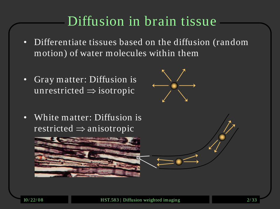
Diffusion in brain tissue

• Gray matter: Diffusion is unrestricted ⇒ isotropic

• White matter: Diffusion is restricted ⇒ anisotropic

• Differentiate tissues based on the diffusion (random motion) of water molecules within them


Diffusion MRI

• Magnetic resonance imaging can provide “diffusion encoding”

• Magnetic field strength is varied by gradients in different directions

• Image intensity is attenuated depending on water diffusion in each direction

• Compare with baseline images to infer on diffusion process No

diffusion encoding

Diffusion encoding in direction g1

g2g3

g4g5

g6


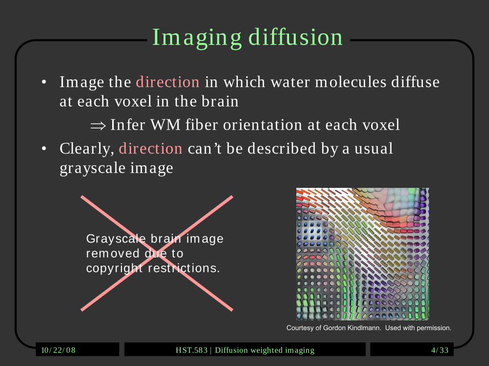
Imaging diffusion

• Image the direction in which water molecules diffuse at each voxel in the brain

⇒ Infer WM fiber orientation at each voxel

• Clearly, direction can’t be described by a usual grayscale image

Grayscale brain image removed due to copyright restrictions.

Courtesy of Gordon Kindlmann. Used with permission.


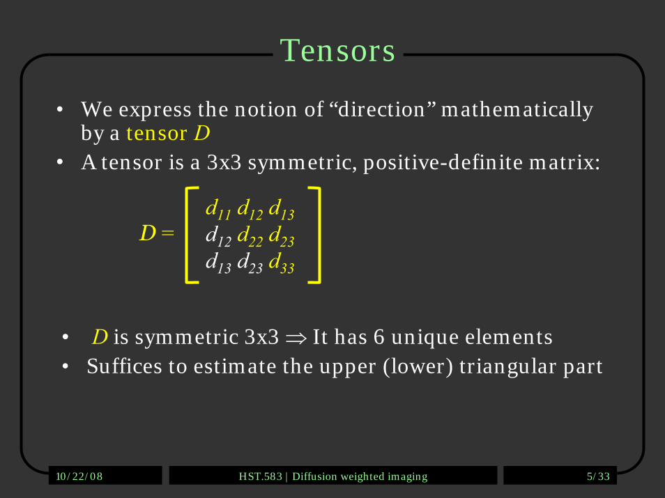
Tensors

• We express the notion of “direction” mathematically by a tensor D

• A tensor is a 3x3 symmetric, positive-definite matrix:

• D is symmetric 3x3 ⇒ It has 6 unique elements• Suffices to estimate the upper (lower) triangular part

d11 d12 d13d12 d22 d23d13 d23 d33

D =


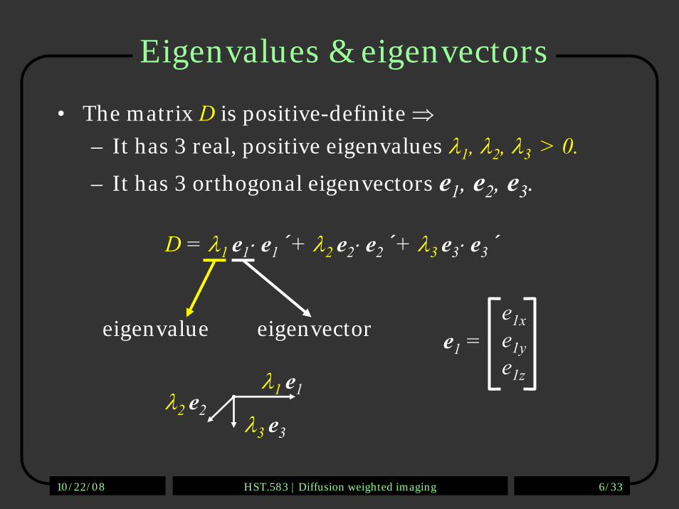
Eigenvalues & eigenvectors

• The matrix D is positive-definite ⇒– It has 3 real, positive eigenvalues λ1, λ2, λ3 > 0.– It has 3 orthogonal eigenvectors e1, e2, e3.

D = λ1 e1⋅ e1´ + λ2 e2⋅ e2´ + λ3 e3⋅ e3´

eigenvaluee1xe1ye1z

e1 =eigenvector

λ1 e1λ2 e2

λ3 e3


Physical interpretation

• Eigenvectors express diffusion direction

• Eigenvalues express diffusion magnitude

λ1 e1

λ2 e2λ3 e3

λ1 e1λ2 e2

λ3 e3

Isotropic diffusion:λ1 ≈ λ2 ≈ λ3

• One such ellipsoid at each voxel: Likelihood of water molecule displacements at that voxel

Anisotropic diffusion:λ1 >> λ2 ≈ λ3


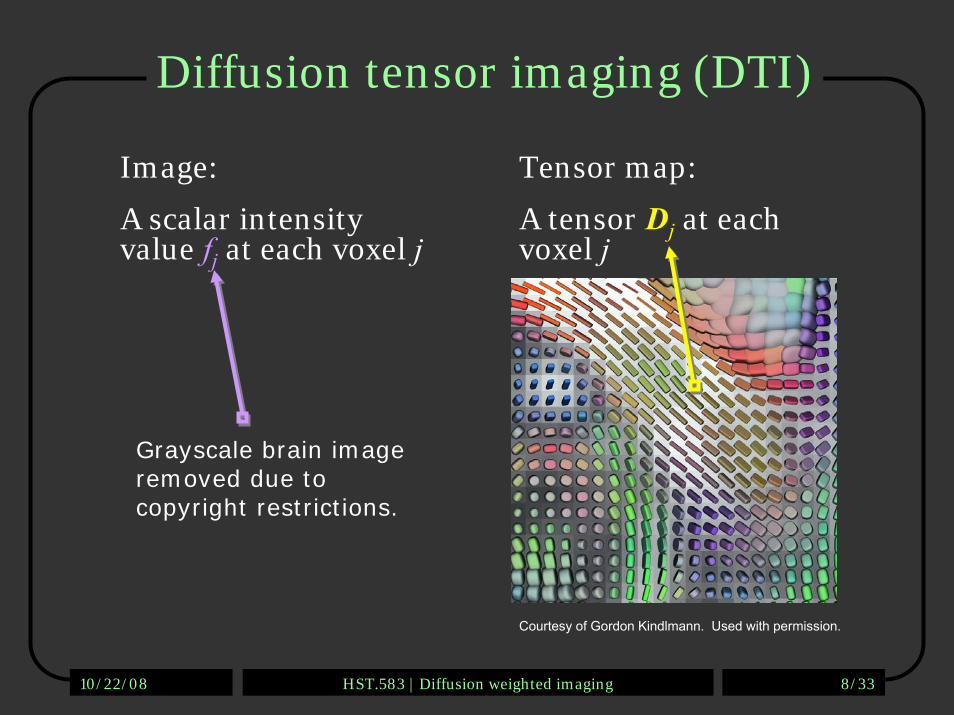
Diffusion tensor imaging (DTI)

Image:

A scalar intensity value fj at each voxel j

Tensor map:

A tensor Dj at each voxel j

Grayscale brain image removed due to copyright restrictions.

Courtesy of Gordon Kindlmann. Used with permission.


Summary measures

• Mean diffusivity (MD):Mean of the 3 eigenvalues

• Fractional anisotropy (FA):Variance of the 3 eigenvalues, normalized so that 0≤ (FA) ≤1

Fasterdiffusion

Slowerdiffusion

Anisotropicdiffusion

Isotropicdiffusion

[λ1(j)-MD(j)]2 + [λ2(j)-MD(j)]2 + [λ3(j)-MD(j)]2

FA(j)2 =λ1(j)2 + λ2(j)2 + λ3(j)2

MD(j) = [λ1(j)+λ2(j)+λ3(j)]/3

3

2


More summary measures

• Axial diffusivity: Greatest eigenvalue

• Radial diffusivity: Average of 2 lesser eigenvalues

• Inter-voxel coherence: Average angle b/w the major eigenvector at some voxel and the major eigenvector at the voxels around it

AD(j) = λ1(j)

RD(j) = [λ2(j) + λ3(j)]/2


Other models of diffusion• The tensor is an imperfect model: What if more than

one major diffusion direction in the same voxel?

• High angular resolution diffusion imaging (HARDI)

– A mixture of the usual (“rank-2”) tensors [Tuch’02]

– A tensor of rank > 2 [Frank’02, Özarslan’03]

– An orientation distribution function [Tuch’04]

– A diffusion spectrum (DSI) [Wedeen’05]

• More parameters at each voxel ⇒ More data needed


Example: DTI vs. DSI

Source: Wedeen, V. J. et al., “Mapping complex tissue architecture with diffusion spectrum magnetic resonance imaging.” MRM 54, no. 6 (2005): 1377-1386. Copyright (c) 2005 Wiley-Liss, Inc., a subsidiary of John Wiley & Sons, Inc. Reprinted with permission of John Wiley & Sons., Inc.


Back to the tensor

• Remember: A tensor hassix unique values

d11

d13d12

d22d23d33

• Must estimate six times as many values at each voxel

⇒ Must collect (at least) six times as much data!

d11 d12 d13d12 d22 d23d13 d23 d33

D =


MR data acquisition

Measure raw MR signal(frequency-domain samples of transverse magnetization)

Reconstruct an image oftransverse magnetization


Diffusion MR data acquisition

Must acquire at least 6 times as many MR signal measurements

Need to reconstruct 6 times as many values

⇐

d11

d13d12

d22d23d33


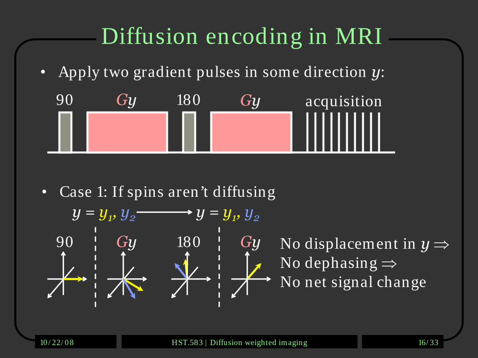
Diffusion encoding in MRI• Apply two gradient pulses in some direction y:

90� 180�Gy Gy

• Case 1: If spins aren’t diffusingy = y1, y2 y = y1, y2

90� 180�Gy Gy No displacement in y ⇒No dephasing ⇒No net signal change

acquisition


Diffusion encoding in MRI• Apply two gradient pulses:

90� 180�Gy Gy

• Case 2: If spins are diffusing

90� 180�Gy Gy

y = y1, y2

Displacement in y ⇒Dephasing ⇒Signal attenuation

y = y1 + Δy1, y2 + Δy2

acquisition


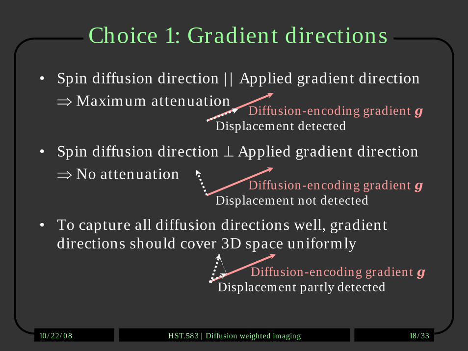
Choice 1: Gradient directions

• Spin diffusion direction || Applied gradient direction

⇒ Maximum attenuation

• Spin diffusion direction ⊥ Applied gradient direction

⇒ No attenuation

• To capture all diffusion directions well, gradient directions should cover 3D space uniformly

Diffusion-encoding gradient gDisplacement detected

Diffusion-encoding gradient gDisplacement not detected

Diffusion-encoding gradient gDisplacement partly detected


How many directions?

• Acquiring with more gradient directions leads to:

+ More reliable estimation of diffusion measures

– Increased imaging time ⇒ Subject discomfort, more susceptible to artifacts due to motion, respiration, etc.

• DTI:

– Six directions is the minimum

– Usually a few 10’s of directions

– Diminishing returns after a certain number [Jones, 2004]

• HARDI/DSI:

– Usually a few 100’s of directions


Choice 2: The b-value

• The b-value depends on acquisition parameters:

b = γ2 G2 δ2 (Δ - δ/3)– γ the gyromagnetic ratio

– G the strength of the diffusion-encoding gradient

– δ the duration of each diffusion-encoding pulse

– Δ the interval b/w diffusion-encoding pulses

90� 180� acquisition

G

Δ

δ


How high b-value?

• Increasing the b-value leads to:

+ Increased contrast b/w areas of higher and lower diffusivity in principle

– Decreased signal-to-noise ratio ⇒ Less reliable estimation of diffusion measures in practice

• DTI: b ~ 1000 sec/mm2

• HARDI/DSI: b ~ 10,000 sec/mm2

• Data can be acquired at multiple b-values for trade-off

• Repeat acquisition and average to increase signal-to-noise ratio


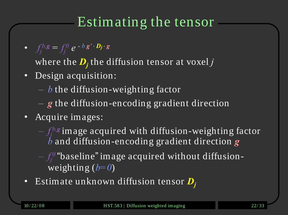
Estimating the tensor

• fjb,g = fj

0 e - b g′ ⋅ Dj ⋅ g

where the Dj the diffusion tensor at voxel j• Design acquisition:

– b the diffusion-weighting factor

– g the diffusion-encoding gradient direction

• Acquire images:

– fjb,g image acquired with diffusion-weighting factor

b and diffusion-encoding gradient direction g– fj

0 “baseline” image acquired without diffusion-weighting (b=0)

• Estimate unknown diffusion tensor Dj


Noise in diffusion-weighted images

• Due to signal attenuation by diffusion encoding, signal-to-noise ratio in DW images can be an order of magnitude lower than “baseline” image

• Eigenvalue decomposition is sensitive to noise, may result in negative eigenvalues

Baselineimage

DWimages


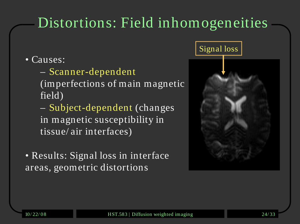
Distortions: Field inhomogeneities

• Causes:– Scanner-dependent(imperfections of main magnetic field)– Subject-dependent (changes in magnetic susceptibility in tissue/air interfaces)

• Results: Signal loss in interface areas, geometric distortions

Signal loss


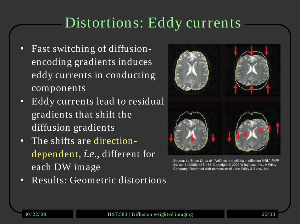
Distortions: Eddy currents

• Fast switching of diffusion-encoding gradients induces eddy currents in conducting components

• Eddy currents lead to residual gradients that shift the diffusion gradients

• The shifts are direction-dependent, i.e., different for each DW image

• Results: Geometric distortions

Source: Le Bihan D., et al. “Artifacts and pitfalls in diffusion MRI.” JMRI24, no. 3 (2006): 478-488. Copyright © 2006 Wiley-Liss, Inc., A Wiley Company. Reprinted with permission of John Wiley & Sons., Inc.


Distortion correction

Post-process images to reduce distortions due to field inhomogeneities and eddy-currents:

– Either register distorted DW images to an undistorted (non-DW) image [Haselgrove’96, Bastin’99, Horsfield’99, Andersson’02, Rohde’04, Ardekani’05, Mistry’06]

– Or use information on distortions from separate scans (field map, residual gradients)[Jezzard’98, Bastin’00, Chen’06; Bodammer’04, Shen’04]


Tractography

• Challenges in tractography:- Noisy, distorted images- Pathway crossings- High-dimensional space

• Many methods to overcome them…

???

• What does one do with diffusion data?

– Statistical analysis on MD, FA, tensors…

– Tractography: Given the diffusion data, determine “best” pathway between two brain regions


Deterministic vs. probabilistic

• Deterministic methods:Model geometry of diffusion data, e.g., tensor/eigenvectors [Conturo ‘99, Jones ‘99, Mori ‘99, Basser ‘00, Catani ‘02, Parker ‘02, O’Donnell ‘02, Lazar ‘03, Jackowski ‘04, Pichon ‘05, Fletcher ‘07, Melonakos ‘07, …]

???

• Probabilistic methods:Also model statistics of diffusion data [Behrens ‘03, Hagmann ‘03, Pajevic ‘03, Jones ‘05, Lazar ‘05, Parker ‘05, Friman ‘06, Jbabdi ‘07, …]


Local vs. global

• Local: Uses local information to determine next step, errors propagate from areas of high uncertainty

• Global: Integrates information along the entire path


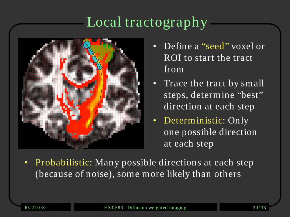
Local tractography

• Define a “seed” voxel or ROI to start the tract from

• Trace the tract by small steps, determine “best”direction at each step

• Deterministic: Only one possible direction at each step

• Probabilistic: Many possible directions at each step (because of noise), some more likely than others


Some issues

• Not constrained to a connection of the seed to a target region

• How do we isolate a specific connection? We can set a threshold, but how?

• What if we want a non-dominant connection? We can define waypoints, but there’s no guarantee that we’ll reach them.

• Not symmetric between tract “start” and “end” point


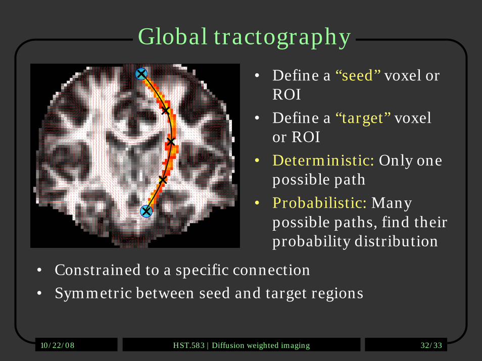
Global tractography

• Define a “seed” voxel or ROI

• Define a “target” voxel or ROI

• Deterministic: Only one possible path

• Probabilistic: Many possible paths, find their probability distribution

• Constrained to a specific connection

• Symmetric between seed and target regions


Application: Huntington’s diseaseData courtesy of Dr. D. Rosas, MGH

Healthy Huntington’s (premanifest) Huntington’s (advanced)

hst.583 functional magnetic resonance imaging: … director: dr. randy gollub. 10/22/08 hst.583 ......

Documents