Low-Latency Trading

Joel Hasbrouck and Gideon Saar

This version: October 2, 2010

Joel Hasbrouck is from the Stern School of Business, 44 West 4th

Street, New York, NY 10012 (Tel: 212-

998-0310, jhasbrou@stern.nyu.edu). Gideon Saar is from the Johnson Graduate School of Management,

Cornell University, 455 Sage Hall, Ithaca, NY 14853 (Tel: 607-255-7484, gs25@cornell.edu). We are

grateful for comments from seminar (or conference) participants at Arhuus University, Humbolt

University, New York University, the Chicago Quantitative Alliance / Society of Quantitative Analysts, the

Investment Industry Regulatory Organization of Canada / DeGroote School, and the World Federation of

Stock Exchanges Statistics Advisory Group.

Low-Latency Trading

Abstract

This paper studies market activity in the ―millisecond environment,‖ where computer

algorithms respond to each other almost instantaneously. Using order-level NASDAQ

data, we find that the millisecond environment consists of activity by some traders who

respond to market events (like changes in the limit order book) within roughly 2-3 ms,

and others who seem to cycle in wall-clock time (e.g. access the market every second).

We define low-latency activity as strategies that respond to market events in the

millisecond environment, the hallmark of proprietary trading by a variety of players

including electronic market makers and statistical arbitrage desks. We construct a

measure of low-latency activity by identifying ―strategic runs,‖ which are linked

submissions, cancellations, and executions that are likely to be parts of a dynamic

strategy. We use this measure to study the impact that low-latency activity has on market

quality both during normal market conditions and during a period of declining prices and

heightened economic uncertainty. Our conclusion is that increased low-latency activity

improves traditional market quality measures such as short-term volatility, spreads, and

displayed depth in the limit order book.

1

I. Introduction

Our financial environment is characterized by the ever increasing pace of both

information gathering and the actions prompted by this information. Speed is important

to traders in financial markets for two main reasons. First, the inherent fundamental

volatility of financial securities means that rebalancing positions faster could result in

higher utility. Second, irrespective of the absolute speed, being faster than other traders

can create profit opportunities by enabling a prompt response to news or market-

generated events. This latter consideration appears to drive an ―arms race‖ where traders

employ cutting-edge technology and locate computers in close proximity to the trading

venue in order to cut down on the latency of their orders and gain an advantage. As a

result, today‘s markets experience intense activity in the ―millisecond environment,‖

where computer algorithms respond to each other at a pace 100 times faster than it would

take for a human trader to blink.

While there are many definitions for the term ―latency,‖ we view it in the context

of the time it takes to observe a market event (e.g., a new bid price in the limit order

book), through the time it takes to analyze this event and send an order to the exchange

that responds to the event.1 Exchanges have been investing heavily in upgrading their

systems to reduce the time it takes to send information to customers as well as to accept

and handle customers‘ orders. They also began offering traders the ability to co-locate

their computer systems in close proxy to the exchange‘s system, reducing the time it

takes for messages to reach customers to less than a millisecond (a thousand of a second).

As traders have also invested in the technology to process information faster, the entire

information-processing-action cycle has been reduced by some traders to a few

milliseconds.

1 More specifically, we define latency as the sum of three components: the time it takes for information to

reach the trader, the time it takes for the trader‘s algorithms to analyze the information, and the time it takes

for the generated action to reach the exchange and get implemented. The latencies claimed by many trading

venues, however, are usually defined much more narrowly, typically as the processing delay measured

from the entry of the order (at the vendor‘s computer) to the transmission of an acknowledgement (from the

vendor‘s computer).

2

An important question is who benefits from such massive investment in

technology. After all, most trading is a zero sum game, and the reduction in fundamental

risk mentioned above would seem incomprehensibly small for time intervals in the order

of several milliseconds. There is a new set of traders in the market who implement low-

latency strategies, which we define as strategies that respond to market events in the

millisecond environment. These traders now generate most message activity in financial

markets and according to some accounts also take part in the majority of the trades.2

While it appears that intermediated trading is on the rise (with these low-latency traders

providing liquidity to other market participants), it is unclear whether low-latency activity

harms or helps market quality.

Our goal in this paper is to examine the influence of these low-latency traders on

the market environment. We begin by studying the millisecond environment to ascertain

how low-latency strategies affect the time-series properties of market activity. We then

ask the following question: how does the interaction of these traders in the millisecond

environment impact the quality of markets that human investors can observe? In other

words, we would like to know how their activity aggregates to affect attributes such as

the short-term volatility of stocks, the total price impact of trades, and the depth of the

market. To investigate these questions, we utilize NASDAQ order-level data (TotalView-

ITCH) that are identical to those supplied to subscribers, providing real-time information

about orders and executions on the NASDAQ system. Each entry (submission,

cancellation, or execution of an order) is time-stamped to the millisecond, and hence

these data provide a very detailed view of activity on the NASDAQ system.

We find that the millisecond environment shows evidence of two types of

activities: one by traders who respond to market events and the other by traders who

seem to operate according to a schedule (e.g., access the market every second). The

activity of the latter creates periodicities in the time-series properties of market activity

based on wall-clock time. We believe that low-latency activity (i.e., strategies that

2 See, for example, the discussion of high-frequency traders in the SEC‘s Concept Release on Equity

Market Structure.

3

respond to market events) is the hallmark of proprietary trading by electronic market

making firms as well as statistical arbitrage operations in hedge funds and other financial

firms. On the other hand, the periodicity is more likely generated by the activity of

agency algorithms employed to minimize trading costs of buy-side money managers. The

interaction among different types of algorithms gives rise to intense episodes of

submissions and cancellations of limit orders that start and stop abruptly, but these need

not lead to intensified trading in the stocks. In other words, observing these episodes

reveals that intense high-frequency activity in the millisecond environment need not

translate into a surge in high-frequency trading.

We use the data to construct ―strategic runs‖ of linked messages that describe

dynamic order placement strategies. By tracking submissions, cancellations, and

executions that can be associated with each other, we create a measure of low-latency

activity. We use a simultaneous equation framework to examine how the intensity of low-

latency activity affects market quality measures. We find that an increase in low-latency

activity lowers short-term volatility, reduces quoted spreads and the total price impact of

trades, and increases depth in the limit order book. If our econometric framework

successfully corrects for the simultaneity between low-latency activity and market

attributes, then the activity of low-latency traders is beneficial by traditional standards

about which investors care.

Furthermore, we employ two distinct sample periods to investigate whether the

impact of low-latency trading on market quality (and the millisecond environment in

general) differs between ―normal times‖ and periods of declining prices and heightened

uncertainty in the market. Our first sample period, October 2007, is characterized by a

relatively flat (or slightly increasing) market. Our second sample period, June 2008, is

characterized by declining prices (the NASDAQ was down 8% in that month) and high

uncertainty following the fire sale of Bear Sterns. We find that the millisecond

environment with its various attributes is rather similar across the two sample periods.

More importantly, low-latency activity enhances market quality is both environments

4

though during stressful times it appears to help reduce volatility in smaller stocks more

than it does in larger stocks.3

Our paper relates to the small but growing strands in the literature on speed in

financial markets as well as on algorithmic trading. In particular, Riordan and

Storkenmaier (2008), Easley, Hendershott, and Ramadorai (2009), and Hendershott and

Moulton (2009) examine market-wide changes in technology that affect the latency of

information transmission and execution, but reach conflicting conclusions as to the

impact of such changes on market quality. There are several papers on algorithmic

trading that characterize the trading environment on the Deutsche Boerse (Gsell (2008),

Gsell and Gomber (2008), Groth (2009), Prix, Loistl, and Huetl (2007), Hendershott and

Riordan (2009)), and two papers that study U.S. markets: Hendershott, Jones, and

Menkveld (2009) and Brogaard (2010). None of these papers study the characteristics of

the millisecond environment, but the latter two papers attempt to evaluate the impact of

algorithmic trading on market quality in the U.S., a goal we share as well.4

The rest of this paper proceeds as follows. The next section describes the sample

and the dataset we use. Section III characterizes the new trading environment. We

provide evidence on the intensity, periodicity, and episodic nature of activity in the

―millisecond environment,‖ and construct a measure of low-latency activity by linking

orders to strategic runs that represent dynamic strategies. Section IV studies how the

activity of low-latency traders in the millisecond environment influences attributes of

market quality such as liquidity and short-term volatility. In Section V we discuss related

papers and how our findings fit within the context of the literature. Section VI concludes

the paper with a discussion of low-latency trading from the perspectives of market

microstructure and the regulatory environment.

3 We note that this does not imply that the activity of low-latency traders would help curb volatility during

extremely brief episodes such as the ―flash crash‖ of May 2010, in which the market declined by about 7%

over a 15-minute interval before partially rebounding. 4 The joint CFTC/SEC report on the ―flash crash‖ of May 6, 2010, looks at the role of high-frequency

trading in this extreme episode (U. S. Commodity Futures Trading Commission and the U.S. Securities and

Exchange Commission, 2010). Although much can be learned from extreme events, our study, in contrast,

uses sample periods that are longer and arguably more representative.

5

II. Data and Sample

II.A. NASDAQ Order-Level Data

The NASDAQ Stock Market is a pure agency market. It operates an electronic limit order

book that utilizes the INET architecture (which was purchased by NASDAQ in 2005).5

All submitted orders must be price-contingent (i.e., limit orders), and traders who seek

immediate execution need to price the limit orders to be marketable (e.g., a buy order

priced at or above the prevailing ask price). Traders can designate their orders to display

in the NASDAQ book or mark them as ―non-displayed,‖ in which case they reside in the

book but are invisible to all traders. Execution priority follows price, visibility, and time.

All displayed quantities at a price are executed before non-displayed quantities at that

price can trade.

The NASDAQ data we use, TotalView-ITCH, are identical to those supplied to

subscribers, providing real-time information about orders and executions on the

NASDAQ system. These data are comprised of time-sequenced messages that describe

the history of trade and book activity. Each message is time-stamped to the millisecond

(i.e., one-thousand of a second), and hence these data provide a detailed picture of the

trading process and the state of the NASDAQ book. We are able to observe four different

types of messages in the TotalView-ITCH dataset: (i) the addition of a displayed order to

the book, (ii) the cancellation of a displayed order, (iii) the execution of a displayed

order, and (iv) the execution of a non-displayed order.

With respect to executions, we believe that the meaningful economic event is the

arrival of the marketable order. In the data, when an incoming order executes against

multiple standing orders in the book, separate messages are generated for each standing

order. We view these as single marketable order arrival, so we group as one event

multiple execution messages that have the same millisecond time stamp, are in the same

direction, and occur in a sequence unbroken by any non-execution message. The

component executions need not occur at the same price, and some (or all) of the

executions may occur against non-displayed quantities.

5 See Hasbrouck and Saar (2009) for a more detailed description of the INET market structure.

6

II.B. Sample

Our sample is constructed to capture variation across firms and across market conditions.

We begin by identifying all common, domestic stocks in CRSP that are NASDAQ-listed

in the last quarter of 2007.6 We then take the top 500 stocks, ranked by market

capitalization as of September 30, 2007. Our first sample period is October of 2007 (23

trading days). The market was relatively flat during that time, with the S&P 500 Index

starting the month at 1,547.04 and ending it at 1549.38. The NASDAQ Composite Index

was relatively flat but ended the month up 4.34%. Our 2007 sample is intended to reflect

a ―normal‖ market environment.

Our second sample period is June 2008 (21 trading days), which represents a time

of heightened uncertainty in the market between the fire sale of Bear Sterns in March of

2008 and the Chapter 11 filing of Lehman Brothers in September of that year. During the

month of June, the S&P 500 Index lost 7.58%, and the NASDAQ Composite Index was

down 7.99%. In the second period, we continue to follow the firms in the 2007 sample,

less 29 stocks that were acquired or switched primary listing. For brevity, we refer to the

October 2007 and June 2008 samples as ―2007‖ and ―2008,‖ respectively.

In our dynamic analysis we use summary statistics constructed over 10-minute

intervals. To ensure the accuracy of these statistics, we impose a minimum message

count cutoff. A firm is excluded from a sample if more than ten percent of the 10-minute

intervals had fewer than 250 messages. Google and Apple are excluded due to

computational limitations. Net of these exclusions, the 2007 sample contains 345 stocks,

and the 2008 sample contains 394 stocks.

Table 1 provides summary statistics for the stocks in both sample periods using

information from CRSP and the NASDAQ dataset. Panel A summarizes the measures

obtained from CRSP. In the 2007 sample, market capitalization ranges from $789 Million

to $276 Billion, with a median of slightly over $2 Billion. The sample also spans a range

of trading activity and price levels. The most active stock exhibits an average daily

6 NASDASQ introduced the three-tier initiative for listed stocks in July of 2006. We use CRSP‘s

NMSIND=5 and NMSIND=6 codes to identify eligible NASDAQ stocks for the sample (which is roughly

equivalent to the former designation of ―NASDAQ National Market‖ stocks).

7

volume of 77 million shares; the median is about one million shares. Average closing

prices range from $2 to $272 with a median of $29. Panel B summarizes data collected

from NASDAQ. In 2007 the median firm had 27,130 order submissions (daily average),

24,374 cancellations and 2,489 executions. Statistics for the 2008 sample are similar.

III. Characterizing the New Trading Environment

III.A. Intensity, periodicity, and High-Frequency Episodes

III.A.a Intensity

Current market observers often comment on the rapid pace of activity. In fact, the typical

average message rate is unremarkable. The sum of the median number of submissions

and cancellations for 2007 is 66,587. With 23,400 seconds in a 6.5 hour trading session, a

representative average message arrival rate appears to be roughly three messages per

second.

The average, however, belies the intensely episodic nature of the activity. To

illustrate this, we estimate the hazard rate for the inter-message durations. The hazard rate

is the message arrival intensity (for a given stock), conditional on the time elapsed since

the last message (for that stock). Figure 1 depicts graphs of the hazard functions for two

types of messages: (i) those that do not involve the execution of trades (arrivals and

cancellations of nonmarketable limit orders), and (ii) executions of trades (against both

displayed and non-displayed limit orders). Panel A presents the hazard rates up to 100

ms, while Panel B shows the hazard rates up to 1000 ms (i.e., one second). The hazard

rates we observe in the market exhibit three striking characteristics: a very high initial

level, a rapid decline, and (in the case of non-execution events) a small number of

apparent peaks.

In the first millisecond (after the preceding message) the hazard rate for

submissions/cancellations is 334 messages per second in 2007, and 283 messages per

second in 2008, i.e., roughly one hundred times the average arrival intensity. These high

values, however, rapidly dissipate. In 2008, the initial hazard rate drops by about 90

percent in the first ten milliseconds, and by about 98% in the first hundred milliseconds.

8

A declining hazard rate is consistent with event clustering. This is a common

feature of financial data, and is often modeled statistically by dependent duration models

(e.g., Engle and Russell (1998), and Hautsch (2004)). From an economic perspective,

variation in trading intensity has long been believed to reflect variation in information

intensity. While the information can be diverse in type and origin, it is often viewed as

relating to the fundamental value of the stock and originating from outside the market

(e.g., a news conference with the CEO or a change in an analyst‘s earnings forecast). At

horizons of extreme brevity, however, there is simply not sufficient time for an agent to

be reacting to anything except very local market information. The information is about

whether someone is interested in buying or selling, and it may lead to a transient price

movement rather than a permanent shift.

While the hazard rate graphs are dominated by the rapid decay, they also exhibit

local peaks. Over the very short run (Panel A), submissions/cancellations have distinct

peaks in both the 2007 and 2008 samples at 60 ms. There are also discernible peaks at 11-

12 ms. These are somewhat less visible because they occur in a region dominated by the

rapid decay. They are nevertheless about 25% higher than the average surrounding

values. These peaks do not appear as distinctly in the execution hazard rates. The latter,

however, also peak around 2-3 ms, a feature discussed in more detail below. Over a

longer interval (Panel B), submissions/cancellations exhibit peaks around 100 and

(partially visible) 1,000 ms.

What do these peaks represent? The peaks at 60, 100 and 1,000 ms correspond to

―natural‖ rates (1,000 times per minute, ten times per second, and once per second), and

so may reflect algorithms that access the market periodically. The peaks at shorter

durations, however, may represent strategic responses to market events, and so serve as

useful indications of effective latency. Both possibilities warrant further investigation.

We turn next to the periodicities, deferring the analysis of strategic responses to Section

III.C.

9

III.A.b Periodicity

To further characterize the periodicities, we examine the level of activity in wall-clock

time (the hazard rate analyses are effectively set in event time). The timestamps in the

data are milliseconds past midnight. Therefore for a given timestamp t, the quantity

mod ,1000t is the millisecond remainder, i.e., a millisecond time stamp within the

second. Assuming that message arrival rates are constant or (if stochastic) well-mixed

within a sample we would expect the millisecond remainders to be uniformly distributed

over the integers {0,1,…,999}.

The data, however, tell a different story. Panel A of Figure 2 depicts the sample

distribution of the millisecond remainders. The null hypothesis is indicated by the

horizontal line at 0.001. The distributions in both sample periods exhibit marked

departures from uniformity. Both feature strong peaks occurring shortly after the one-

second boundary (at roughly 10-30 ms.), and also around 150 ms. Broad elevations occur

around 600 ms. We believe that these peaks are indicative of automated trading systems

that periodically access the market, near the second and the half-second. These intervals

are substantially longer than the sub-100 ms horizon that characterizes the elevated

hazard rates.

In other words, unlike low-latency traders who respond to market-created events,

these algorithms submit a message and revisit it at fixed intervals. For example, if an

algorithm were to revisit the possibility of modifying an order every five calendar

seconds, we would observe that the algorithm revises the message at 5 ms or 15 ms or 55

ms depending on how fast it sends a message (e.g., cancellation, submission) to the

market. In other words, we observe several peaks rather than one probably due to

differences in the location of traders (e.g., the round-trip New York to Chicago

transmission time is about twelve milliseconds) and the computing technology they

utilize. Algorithms that cycle every half a second could be generating the peak at the 550

reminder.

To investigate whether there might exist longer periodicities, we construct the

sample distribution of timestamps mod 10,000 (Figure 2, Panel B). These graphs are

10

dominated by the strong one-second cycles, but also appear to contain two- and ten-

second variations.

One could suggest that even if a significant fraction of market participants were to

have their algorithms cycle in a one-second frequency, the occurrence times would be

more smoothly distributed due to randomness in clock synchronizations. We believe,

however, that the periodicity can be initiated even by a few, relatively large, market

participants. Furthermore, as long as someone is sending messages in a periodic manner,

their actions will provoke strategic responses by others who monitor the market

continuously (the low-latency traders) and these responses will tend to amplify the

periodicity.

III.A.c High-Frequency Episodes

Both the short-term intensity dependence and clock-time periodicity could in principle be

modeled statistically with standard time series decomposition techniques. Our attempts to

accomplish this (with spectral and wavelet analysis), however, were not very fruitful.

Despite this, certain idiosyncrasies of the decompositions did reveal to us another

characteristic of the millisecond environment. Much high-frequency activity is not only

episodic, but is also strikingly abrupt in commencement and completion.

Panel A of Figure 3 shows both submissions and cancellations (the bars) and

cumulative executions (the dashed line) for ticker symbol INWK (InnerWorkings Inc.) on

June 2, 2008 at about 2:08pm.7 The first noteworthy feature of this figure is that the burst

of high-frequency submissions and cancellations (around 100 messages per second) starts

suddenly and stops abruptly after about one minute and forty seconds. The level of

activity during this time is over 100 times the level of activity in terms of submissions

and cancellations before and after the episode. The second noteworthy feature of the

7 One could identify these episodes simply by looking at (many) plots of submission and cancellation

counts. Our attention was drawn to them, however, by wavelet decompositions that flagged particularly

strong components in message activity at various frequencies. Measures we constructed from the wavelet

analysis were unable to consistently characterize the intensity of low-latency responses to market events,

but they quickly located the instances of high-frequency activity discussed here.

11

figure is that the number and pattern of executions (in the dashed line) does not change

much during this high-frequency episode.

Panel B of Figure 3 shows another such episode in ticker symbol SANM

(Sanmina-SCI Corp.) on June 17, 2008 at around 12:07pm, while Panel C of the figure

presents an episode in GNTX (Gentex Corp.) on June 12, 2008 at around 12:18pm. They

all share the same features: (i) a sudden onset of intense activity of submissions and

cancellations of limit orders that stops abruptly after a short period of time, and (ii) lack

of change in the pattern of executions before, during, or after these high-frequency

episodes. These figures suggest to us that the term ―high-frequency trading‖ that is used

to describe some low-latency activity is generally a misnomer: there is indeed high-

frequency activity, but it does not lead necessarily to intense trading. It simply manifests

in intense submissions and cancellations of orders. And while the episodes in Figure 2

last from one minute and twenty seconds to three minutes, other episodes we have

observed could last only a couple of seconds but contain thousands of messages.8

The millisecond environment therefore consists of activity by some traders who

respond to market events and others who seem to cycle in wall-clock time. This activity

could give rise to intense episodes of submissions and cancellations of limit orders that

start and stop abruptly, but these episodes need not be accompanied by intensified trading

in the stocks. Before we proceed to measure low latency trading and investigate its

impact on market quality, it would be useful to have a short discussion of the type of

market participants whose activity shapes the millisecond environment.

III.B. The Players: Proprietary Algorithms and Agency Algorithms

Much trading and message activity in U.S. equity markets is commonly attributed to

trading algorithms.9 However, not all algorithms serve the same purpose and therefore the

8 A recent newspaper article notes that such episodes are called ―quote stuffing‖ by practitioners (Lauricella

and Strasburg (2010)). Some suspect that these are used by proprietary traders to manipulate prices and

create profit opportunities for executing trades. While this is certainly possible, our observation that there is

no change in the pattern of executions during or immediately after many of these episodes suggests that the

story behind this phenomenon may be more complex. 9 The SEC‘s Concept Release on Equity Market Structure cites media reports that attribute 50% or more of

equity market volume to proprietary algorithms (the ―high-frequency traders‖). A report by the Tabb Group

12

patterns they induce in market data and the impact they have on market quality could

depend on their specific objectives. Broadly speaking, however, we can categorize

algorithmic activity into two separate branches with very different properties: Agency

Algorithms (AA) and Proprietary Algorithms (PA). The first category is comprised of

algorithms used by buy-side institutions to minimize the cost of executing trades in the

process of implementing changes in their investment portfolios. The second category is

comprised of algorithms used by electronic market makers, hedge funds, proprietary

trading desks of large financial firms, and independent statistical arbitrage firms that are

meant to profit from the trading environment itself (as opposed to investing in stocks).10

Agency Algorithms (AA): These are used by buy-side institutions as well as the

brokers who serve them to buy and sell shares. They have been in existence for about two

decades, but the last ten years have witnessed a dramatic increase in their appeal due to

the change to trading in penny increments (in 2001) and increased fragmentation in U.S.

equity markets (following Reg ATS in 1998 and Reg NMS in 2005). These algorithms

break up large orders into pieces that are then sent over time to multiple trading venues.11

The algorithms determine the size, timing, and venue for each piece depending on input

parameters for each order (e.g., the desired horizon for the execution), algorithm-specific

parameters that are estimated from historical data, possibly real-time data received from

the market, and feedback about the execution of the different pieces.

The key characteristic of AA is that the choice of which stock to trade and how

much to buy or sell is made by a portfolio manager who has an investing (rather than

trading) horizon in mind. The algorithms are meant to minimize execution costs relative

to a specific benchmark (e.g., volume-weighted average price or market price at the time

the order arrives at the trading desk), and they are most often developed by sell-side

brokers or independent software vendors to serve buy-side clients. Their ultimate goal is

to execute a desired position change and hence can be viewed as demanding liquidity

(July 14, 2010) suggests that buy-side institutions use ―low-touch‖ agency algorithms for about a third of

their trading needs. 10

Sellberg (2010) refers to these two categories as ―alpha-preserving‖ (agency) and ―alpha-creating‖

(proprietary) algorithms. 11

See, for example, Bergan and Devine (2005).

13

even if they are implemented using a dynamic limit order strategy that utilizes

nonmarketable limit orders.

Proprietary Algorithms (PA): This is a collective name for many strategies and

hence, unlike AA, it is more difficult to have a concise characterization of their nature.

Nonetheless, these algorithms often belong to the following two broad categories: (i)

electronic market making, or (ii) statistical arbitrage trading.

Electronic (or automated) market makers are dealers who buy and sell for their

own account in a list of securities. These firms use algorithms to generate buy and sell

limit orders and dynamically update these orders by applying pre-determined logic to

real-time data. Like traditional dealers, they often profit from the small differences

between the bid and ask prices and aim at carrying only a small inventory. Another

source of profit for such firms is the liquidity rebates offered by many trading venues.

These rebates (typically a quarter of a penny per share) are offered to attract liquidity

providers and are funded by fees that liquidity demanders pay for execution.

Statistical Arbitrage trading is carried out by the proprietary trading desks of

larger financial firms, hedge funds, and independent specialty firms. They analyze

historical data for individual stocks and groups of assets in a search for trading patterns

(within assets or across assets) that can be exploited for profit. These profit opportunities

represent temporary deviations from historical patterns (e.g., pairs trading) or stem from

identification of a certain trading need in the market (e.g., a large trader that attempts to

execute an order and temporarily changes the time-series behavior of prices). Broadly

speaking, most of these strategies rely on convergence of prices and the expectation that

the market price will revert back after temporary imbalances. Some of these traders

attempt to profit from identifying the footprints of buy-side algorithms and trade ahead of

or against them. Their goal is to profit at the expense of buy-side institutions by

employing algorithms that are more sophisticated than typical AA (Donefer (2010)).12

12

The SEC‘s Concept Release on Equity Market Structure provides more information about these strategies

and categorizes them into three groups: arbitrage (usually between related securities or markets), structural

(exploiting market structure features or inference about trading interest), and directional (momentum and

reversal trading based on anticipation of an intraday price movement).

14

The goals of AA and PA differ from each other, and therefore the specifications

of the algorithms and the technology that they require are also dissimilar. AA are based

on historical estimates of price impact and execution probabilities across multiple trading

venues and over time, and often require much less real-time input except for tracking the

pieces of the orders they execute. For example, volume-weighted average price

algorithms attempt to distribute executions over time in proportion to the aggregate

trading and achieve the average price for the stock. While some AA offer functionality

such as pegging (e.g., tracking the bid or ask side of the market) or discretion (e.g.,

converting a nonmarketable limit buy order into a marketable order when the ask price

decreases), typical AA do not require millisecond responses to changing market

conditions.

We believe that the clock-time periodicity we have identified in Section III.A.b is

driven by these AA. Some algorithms simply check market conditions and execution

status every second (or several seconds) and respond to the changes they encounter. Their

orders reach the market with a lag that depends on the configurations and locations of

their computers, generating the sample distributions of remainders. The similarities

between the 2007 and 2008 samples suggest phenomena that are pervasive and do not

disappear over time or in different market conditions.

One might conjecture that these patterns cannot be sustainable because

sophisticated algorithms will take advantage of them and eliminate them. While there is

no doubt that PA respond to such regularities, these responses only serve to accentuate

the clock-time periodicities rather than eliminate them. It is also the case that PA supply

liquidity to AA and therefore it is conceivable that clustering at certain times help AA

execute their orders by increasing available liquidity. As such, AA that operate in

calendar time would have little incentive to change, making these patterns we identify in

the data persist over time.

In contrast to AA, the hallmark of PA is speed: low-latency capabilities. In other

words, what distinguishes them from AA is their need to respond to market events.

Therefore, these algorithms utilize co-location, which is the ability to place computers in

15

close proximity to the stock exchange‘s servers, and special computing technology to

create an edge in the strategic interaction of the millisecond environment. While AA are

used in the service of buy-side investing and hence seem justified by the social benefit

often attributed to delegated portfolio management (e.g., diversification), the societal

benefits of PA are more elusive. If we take electronic market making to be an extension

of traditional market making, it provides the service of bridging the intertemporal

disaggregation of order flow in continuous markets. Unlike traditional dealers, however,

these electronic market making firms have no explicit obligations with respect to market

presence or market quality, an issue we will further discuss in Section VI.

The societal benefit from the statistical arbitrage and other types of low-latency

trading is more difficult to ascertain. One could view them as aiding price discovery by

eliminating transient price disturbances, but such an argument at the millisecond

environment is a bit tenuous. After all, at such speeds and for such short intervals it is

difficult to determine what constitutes a real innovation to the true value of the security as

opposed to a transitory influence on the price. The social utility in identifying buy-side

interest and trading ahead of it is even more difficult to ascertain.

Furthermore, the race to interact with the market environment faster and faster

requires investing vast resources in technology. PA are at the forefront of such

investment, but they are not alone: AA providers respond by creating algorithms that

enable clients to implement somewhat more sophisticated strategies that respond to

market conditions along pre-defined parameters. Even exchanges such as NASDAQ get

into the game by offering clients simple algorithms like pegging or discretionary orders

through a platform that is operated by the exchange and connects directly to the execution

engine.13

Together, these algorithms constitute ―low-latency trading‖ that shapes the

millisecond environment and therefore begs the question whether it harms or improves

market quality along dimensions about which we care outside of the millisecond

13

NASDAQ‘s RASH (Routing and Special Handling) protocol enables clients to use advanced

functionality such as discretion (predetermined criteria for converting standing limit orders to marketable

orders), random reserve (of partially non-displayed limit orders), pegging (to the relevant side of the market

or the midquote), and routing to other trading venues.

16

environment. Answering this question is the goal of Section IV, but as a pre-requisite it

necessitates developing a measure of low-latency activity.

III.C. Responding to the Market Environment

Our definition of low-latency trading is ―strategies that respond to market events in the

millisecond environment.‖ Although any event might be expected to affect all

subsequent events, our interest here is the speed of response. It is therefore reasonable to

focus on conditioning events that seem especially likely to trigger rapid reactions. One

such event is the improvement of a quote. An increase in the bid may lead to an

immediate trade (against the bid) as potential sellers race to hit it. Alternatively,

competing buyers may race to cancel and resubmit their own bids to remain competitive

and achieve or maintain time priority. We call the former response a same-side execution,

and the latter response a same-side submission/cancellation. Sell side events, subsequent

to a decrease in the ask price, are defined similarly.

Our analysis requires only a slight change to the estimation of the hazard rates

depicted in Figure 1. These earlier results are unconditional in the sense that they reflect

durations subsequent to events of all types. The present characterization focuses on

hazard rates subsequent to order submissions that improve the quote. Figure 4 (Panel A)

depicts the conditional hazard rates for same-side events (pooled over bid increases and

ask decreases).

In the discussion of Figure 1, we noted small local peaks at approximately 2-3 ms.

These peaks are much more sharply defined in the conditional analysis, particularly for

executions. This suggests that the fastest responders are subject to 2-3 ms latency. For

comparison purposes, we note that human reaction times are generally thought to be on

the order of 200 milliseconds (Kosinski (2010)). Therefore, it is a reasonable to assume

that these responses represent actions by automated agents (various types of trading

algorithms). The figure suggests that the time it takes for some low-latency traders to

observe the market event, process the information, and act on it is indeed very short.

17

The hazard rates depicted in Panel B of Figure 4 are conditional on an order

cancellation that resulted in the deterioration of the quote (a drop in the bid or increase in

the ask). Peaks at 2-3 ms. are visible for same-side submissions and cancellations,

presumably reflecting the repricing of orders pegged to the same-side quote. For

executions, the peak is very small in 2007 and non-existent in 2008. Perhaps

unsurprising, withdrawal of a bid (for example) does not induce sellers to chase it.

III.D. Strategic Runs

The evidence to this point has emphasized message timing. One would ideally like to

track low-latency activity in order to decipher its impact on the market. Before turning to

the methodology we use to track the algorithms, it is instructive to present two particular

message sets that we believe are typical. It appears that at least some of the activity

consists of algorithms that either ―play‖ with one another or submit and cancel repeatedly

in an apparent attempt to trigger an action on the part of another algorithm.

Panel A of Table 2 is an excerpt from the message file for ticker symbol ADCT

on October 2, 2007 beginning at 09:51:57.849 and ending at 09:53:04.012 (roughly 66

seconds). Over this period, there were 35 submissions (and 35 cancels) of orders to buy

100 shares, and 32 submissions (and 32 cancels) of orders to buy 300 shares. The pricing

of the orders caused the bid quote to rapidly oscillate between $20.04 and $20.05. The

difference in order sizes and the brief intervals between cancelations and submissions

suggest that the traffic is being generated by algorithms that seem to respond to each

other.14

Panel B of Table 2 describes messages (for the same stock on the same day)

between 09:57:18.839 and 09:58:36.268 (about 78 seconds). Over this period, orders to

sell 100 shares were submitted (and quickly cancelled) 142 times. During much of this

period there was no activity except for these messages. As a result of these orders, the ask

quote rapidly oscillated between $20.13 and $20.14.

14

When a similar sequence of events was discussed with a group of practitioners, one person pointed out

that the sequence could have been generated by a single player intending to give the appearance of multiple

competing buyers. Fictitious trades (―wash sales‖) are clearly considered illegal in the US, but this scenario

would not involve trades, only quotes.

18

The underlying logic behind each algorithm that generates such strategic runs of

messages is difficult to reverse engineer. It could be that some algorithms attempt to

trigger an action on the part of other algorithms (e.g., canceling and resubmitting at a

more aggressive price) and then interact with them. Whatever the reasoning, it is clear

that an algorithm that repeatedly submits orders and cancels them within 10 ms does not

intend to interact with human traders (whose response time would probably take more

than 200 ms even if their attention is focused on this particular security). These

algorithms operate in their own space: they are intended to trigger a response from (or

respond to) other algorithms. Activity in the limit order book is dominated nowadays by

this kind of interaction between automated algorithms, in contrast to a decade ago when

human traders still ruled. How, then, are these algorithms affect the environment that the

human traders observe? How is such activity related to market quality measures

computed over minutes rather than milliseconds? In order to answer these questions, we

need to create a measure of the activity of these low-latency traders.

We construct such a measure by identifying ―strategic runs,‖ which are linked

submissions, cancellations, and executions that are likely to be parts of a dynamic

strategy. Since our data do not identify individual traders, our methodology no doubt

introduces some noise into the identification of low-latency activity. We nevertheless

believe that other attributes of the messages can used to infer linked sequences. In

particular, our ―strategic runs‖ (or simply, in this context, ―runs‖) are constructed as

follows. Reference numbers supplied with the data unambiguously link an individual

limit order with its subsequent cancellation or execution. The point of inference comes in

deciding whether a cancellation can be linked to either a subsequent submission of a

nonmarketable limit order or a subsequent execution that occurs when the same order is

resent to the market priced to be marketable. We impute such a link when the

cancellation is followed within one second by a limit order submission or by an execution

in the same direction and for the same quantity. To be eligible for further analysis, we

require that a run have at least one such resubmission.

19

We build the runs forward throughout the day. A limit order or a cancellation can

be associated with only one run. An execution, however, might involve two runs. A

canonical limit order strategy involves an initial submission priced away from the market,

subsequent repricing to make the order more aggressive, and finally (if the order isn‘t

executed) cancellation and resubmission of a marketable order. Thus, the passive side of

an execution might be associated with one run, while the active side might be associated

with another run (in the opposite direction) that became marketable.15

Our procedure linked roughly 60 percent of the cancellations in the 2007 sample,

and 55 percent in the 2008 sample. Although we allow up to a one second delay from

cancellation to resubmission, most resubmissions occur much more promptly. The

median resubmission delay in our runs is one millisecond. The length of a run can be

measured by the number of linked messages. The simplest run would have three

messages, a submission of a nonmarketable limit order, its cancellation, and its

resubmission as a marketable limit order that executes immediately (i.e., an ―active

execution‖). The shortest run that does not involve an execution is a limit order that was

submitted, cancelled, resubmitted, and cancelled or expired at the end of the day. Our

sample periods, however, feature many runs of 10 or more linked messages and the

longest run we identify has 93,243 messages. We identify about 57 million runs in the

2007 sample period and 78 million runs in the 2008 sample period.

Panel A of Table 3 looks at summary statistics for the runs. We observe that

around 80% of the runs have 3 to 9 messages, but the longer runs (10 or more messages)

constitute approximately half of the messages that are associated with strategic runs. The

proportion of runs that were (at least partially) executed is 33.57% in 2007 and 27.34% in

2008. Interestingly, 22.74% of the 2007 runs (17.77% in 2008) achieved passive

executions, that is, when a limit order was hit by an incoming marketable order. This is

15

Of course, we cannot assert that the intent of the active side was to submit a marketable order. A limit

order might be priced slightly short of the best visible opposing quote, and yet achieve execution against a

hidden limit order. In this case, we observe an execution at the price of the hidden order, but we don‘t know

the limit price specified in the order that executed against the hidden order.

20

notable because it can be interpreted as an average fill rate for runs, and stands in contrast

to the fill rate for individual limit orders, which is much lower.16

About 10.95% (9.64%) of the runs in the 2007 (2008) sample period end with a

switch to active execution. That is, a limit order is cancelled and replaced with a

marketable order. These numbers attest to the importance of strategies that pursue

execution in a gradual fashion. In the combined 2007 and 2008 samples there are a total

of 57,848,674 executions. There were (combined) 13,799,814 runs that realized active

executions. Since all runs by definition start with a nonmarketable limit order, we can

determine that 23.9% (13,799,814/57,848,674) of all executions were preceded by an

attempt to obtain a passive execution. This highlights the fluidity with which liquidity

suppliers and demanders, often modeled as distinct populations, can in fact switch roles.

Our methodology to impute links between orders no doubt results in

misclassifications that introduce an error into the analysis. However, we believe that the

longer the run we impute, the more likely it is that it represents the activity of a real low-

latency strategy that responds to market events. In other words, to capture the algorithms

that interact with each other in real time (like those in Table 2) it is best to restrict our

attention to strategic runs beyond a certain number of messages. We therefore use runs of

10 or more messages to construct a measure of low-latency traders that we use in the rest

of the analysis. While the 10-message cutoff somewhat arbitrary, these runs represent

about a half of the total number of messages that are linked to runs in each sample period,

and we also believe that such longer runs characterize the episodes associated with

intense high-frequency activity as in Figure 3.

Panel B of Table 3 shows the elapsed time from the beginning to the end of runs

of 10 or more messages. It is interesting to note that many of the runs between 10 and 99

messages start and end within a tenth of a second (there are 497,317 such runs in 2007

and 180,675 in 2008). Nonetheless, most of these runs evolve over one to ten minutes,

and time to completion of a run in general increases in the number of messages. Still, the

16

The low fill rate of limit orders seems to characterize the modern electronic limit order book

environment. Hasbrouck and Saar (2009) report a fill rate of 7.99% for a 2004 sample of Inet data.

21

intensity of the high-frequency episodes we describe in Figure 3 is reflected in the fact

that many of the very long runs (1000 messages and above) start and end within a single

minute.

IV. Low-Latency Trading and Market Quality

Agents who engage in low-latency trading and interact with the market over millisecond

horizons are at one extreme in the continuum of market participants. Most investors

either cannot or choose not to engage the market at this speed.17

These investors‘

experience with the market is still best described with the traditional market quality

measures in the market microstructure arsenal. Hence, a natural question to ask is how

does low-latency activity with its algorithms that interact in milliseconds relate to depth

in the market or the range of prices that can be observed over minutes or hours? This

question does not have an obvious answer. It seems to resemble the challenge faced by

physicists when attempting to relate quantum mechanics‘ subatomic interactions to our

daily life that appears to be governed by Newtonian mechanics. However, if we believe

that healthy markets need to attract longer-term investors whose beliefs and preferences

are essential for the determination of market prices, then market quality should be

measured using time intervals that are easily observed by these investors.

We therefore seek to characterize the influence of low-latency trading on

measures of liquidity and short-term volatility observed over 10-minute intervals

throughout the day. Measures such as the range between high and low prices in these

intervals, the effective and quoted spreads, and the depth of the exchange‘s limit order

book should give us a sense of market quality. And while we would likely not capture

every instance of PA in each interval of time, the strategic runs we have identified in the

previous section could be used to construct a measure of low-latency activity.

17

The recent SEC Concept Release on Equity Market Structure refers in this context to ―long-term

investors … who provide capital investment and are willing to accept the risk of ownership in listed

companies for an extended period of time‖ (p. 33).

22

IV.A. Measures and Methodology

To measure the intensity of low-latency activity in a stock in each ten-minute interval we

use the time-weighted average of the number of strategic runs of 10 messages or more the

stock experiences in the interval (RunsInProcess).18

Higher values of RunsInProcess

indicate greater low-latency activity.

We use our NASDAQ order-level data to compute several measures that represent

different aspects of market quality: a measure of short-term volatility and three measures

of liquidity. The first measure, HighLow, is defined as the highest midquote in an interval

minus the lowest midquote in the same interval. The second measure, EffSprd, is the

average effective spread (or total price impact) of all trades on NASDAQ during the ten-

minute interval (where the effective spread of a trade is computed as the absolute value of

the difference between the transaction price and the prevailing midquote). The third

measure, Spread, is the time-weighted average quoted spread (ask price minus the bid

price) on the NASDAQ system in an interval. The fourth measure, NearDepth, is the

time-weighted average number of shares in the book up to 10 cents from the best posted

prices.19

Although a ten-minute window is a reasonable interval over which to average the

market quality measures, it is sufficiently long (particularly for the low-latency traders)

that the analysis must confront the issue of simultaneity. For example, while we aim to

test whether low-latency trading affects short-term volatility, it is quite possible that

short-term volatility attracts or deters low-latency activity and hence affects the number

of runs that we can observe in the interval.

To address this problem we propose a two-equation simultaneous equation model

in which one of the endogenous variables is RunsInProcess (our low-latency activity

measure) and the other endogenous variable is the market quality measure (i.e., we

18

The time-weighting of this measure works as follows. Say we construct this variable for the interval

9:50:00am-10:00:00am. If a strategic run started at 9:45:00am and ended at 10:01:00am, it was active for

the entire interval and hence it adds 1 to the RunsInProcess measure. A run that started at 9:45:00am and

ended at 9:51:00am was active for one minute (out of ten) in this interval, and hence adds 0.1 to the

measure. Similarly, a runs that was active for 6 seconds within this interval adds 0.01. 19

We have also conducted all the tests with a depth measure defined as the time-weighted average number

of shares in the book up to 50 cents from the best prices, and the results were similar.

23

estimate the model separately for HighLow, EffSprd, Spread, and NearDepth). This

variable is indicated in the specifications by the placeholder MktQuality. The key to

estimating such a model is to identify an instrument for market quality that does not

directly affect RunsInProcess and an instrument for RunsInProcess that does not directly

affect market quality in the stock.

As an instrument for RunsInProcessi,t (the number of runs of 10 messages or more

in stock i in interval t) we use the average number of runs of 10 messages or more in the

same interval for the other stocks in our sample (excluding stock i), denoted RunsNotIt.

Low-latency activity is determined by the number of players in the low-latency field

(e.g., how many electronic market makers and statistical arbitrage firms are using low-

latency strategies), by the state of the limit order book and stock-specific trading activity

in the interval, and by market conditions that affect how aggressive low-latency firms are

during that time.20

The instrument RunsNotIt is determined by the number of low-latency

firms and how active they are in the market during that interval, but at the same time it

does not utilize information about stock i and hence is not a direct determinant of the

liquidity or volatility of stock i in interval t, rendering it an appropriate instrument.

As an instrument for market quality we use a measure that is closely related to the

liquidity of the stock in the interval, but does not directly determine the number of

strategic runs in that stock. Our chief measure is the dollar effective spread (absolute

value of the distance between the transaction price and the midquote) computed for the

same stock and during the same time interval only from trades executed on other (non-

NASDAQ) trading venues. This variable is denoted EffSprdNotNASi,t, and is computed

using the TAQ database. This instrument reflects the general liquidity of the stock in the

interval, but it does not reflect the activity on NASDAQ and hence would not be directly

determined by the number of strategic runs that are taking place on the NASDAQ system.

To examine the robustness of our result to this specific instrument, we repeat the analysis

20

The ―flash crash‖ on May 6, 2010, could be viewed as an example of how overall market conditions can

affect the aggressiveness of low-latency traders in individual stocks. According to a Wall Street Journal

article by Scott Patterson and Tom Lauricella, several electronic market making firms pulled back from the

market because the market as a whole seemed too volatile.

24

using another instrument with a similar flavor, the time-weighted average quoted spread

from TAQ, excluding NASDAQ quotes (denoted SpreadNotNasi,t).

With these instruments, we use Two-Stage-Least-Squares (2SLS) to estimate the

following two-equation simultaneous equation model for each market quality measure:

, 1 , 2 , 1,

, 1 , 2 , 2,

i t i t i t t

i t i t i t t

MktQuality a RunsInProcess a EffSprdNotNAS e

RunsInProccess b MktQuality b RunsNotI e

where 1,...,i N indexes firms, 1,...,t T indexes 10-minute time intervals, and

MktQuality represents one of the market quality measures: HighLow, EffSpread, Spread,

and NearDepth. All variables are standardized to have zero-mean and unit variance,

obviating the need for intercepts in the specification.

The 2SLS methodology effectively replaces RunsInProcessi,t in the first equation

with the fitted values from the regression of RunsInProcessi,t on the instruments.

Similarly MktQualityi,t in the second equation is replaced with the fitted values of the

regression of MktQualityi,t on the instruments. This gives us a consistent estimate of the

a1 coefficient that tells us how low-latency activity affects market quality. We estimate

the system by pooling observations across all stocks and all time intervals. The

standardization of the variables essentially implements a fixed-effects specification. A

potential disadvantage of pooling is that the errors of different stocks may not be

identically distributed. For robustness, we also report summary measures of the

coefficients from stock-by-stock estimations of the system. While stock-by-stock analysis

does not assume identically distributed errors across stocks, it leaves us with a much

smaller number of observations for each estimation (897 in the 2007 sample period and

819 in the 2008 sample period) and hence has reduced power relative to the pooled time-

series/cross-sectional specification.

IV.B. Results

Panel A of Table 4 presents the estimated coefficients of the pooled system side-by-side

for the 2007 and 2008 sample periods. First we note that the two instruments have the

25

expected signs and are highly significant. Specifically, the coefficient a2 indicates that

when liquidity off NASDAQ is higher, our NASDAQ market quality measures show

higher liquidity and lower volatility. Similarly, the coefficient b2 is positive in all

specifications, indicating that higher low-latency activity in a specific stock in an interval

is associated with higher low-latency activity in other stocks on the NASDAQ system.

Second, the estimated b1 coefficients tell us that low-latency activity is attracted to more

liquid and less volatile stocks.

The most interesting coefficient is a1, which measures the impact of low-latency

activity on the market quality measures. We observe that higher low-latency activity

implies lower posted and effective spreads, greater depth, and lower short-term volatility.

Moreover, the impact of low-latency activity on market quality is similar in the 2007 and

2008 sample periods. The fact that low-latency trading decreases short-term volatility and

contributes to depth in the 2008 sample period where the market is relentlessly going

down and there is heightened uncertainty in the economic environment is particularly

noteworthy. It seems to suggest that PA activity creates a positive externality in the

market at the time that the market needs it the most. Panel B of Table 4 presents roughly

similar results from the estimation of the system with SpreadNotNasi,t as the instrument

for market liquidity.21

It is possible, however, that the impact of low-latency trading on market quality

would differ for stocks that are somehow fundamentally dissimilar, like small versus

large market capitalization stocks. Table 5 presents system estimates in subsamples

consisting of four quartiles ranked by the average market capitalization over the sample

period.22

There is not much pattern across the quartiles in the manner low-latency activity

affects short-term volatility in the 2007 sample period. The picture in the 2008 sample is

different: It appears that during more stressful times, low-latency activity helps reduce

volatility in smaller stocks more than it does in larger stocks.

21

The only difference in the results with SpreadNotNasi,t as the instrument is that the coefficient a1 is not

statistically significant for the EffSprd measure in the 2008 sample period. 22

The results in the table are presented with EffSprdNotNASi,t as the instrument for the market quality

measures. We obtain similar results (with similar patterns across the quartiles) using SpreadNotNasi,t as the

instrument.

26

Another interesting pattern can be observed in the coefficient b1, which tells us

how market quality affects low-latency trading. While low-latency activity increases in

market quality for larger stocks in the 2007 sample period, no such relationship is found

for smaller stocks, where the coefficient has the opposite sign but is not statistically

significant. During the stressful period of June 2008, however, the b1 coefficients suggest

a different behavior: Higher liquidity encourages low-latency trading in smaller stocks

but not in the top quartile of stocks by market capitalization where we observe the

opposite pattern (though the absolute magnitude of the coefficient in large cap stocks is

rather small and hence the effect is probably not very strong).

Lastly, Table 6 shows summary statistics for the stock-by-stock estimations. The

results suggest similar conclusions concerning the effect of low-latency trading on market

quality. In particular, an increase in low-latency activity decreases short-term volatility,

decreases quoted spreads, and increases displayed depth in the limit order book. This is

true both in the 2007 and 2008 sample periods. The median coefficient is insignificant

when the liquidity measure is EffSprd in both sample periods. The only consistent

difference between the pooled estimation and the stock-by-stock analysis is that none of

the median coefficients of b1 is statistically significant. In other words, while the impact

of low-latency trading on market quality seems robust, our finding that low-latency

activity is attracted to more liquid and less volatile stocks should be somewhat qualified

due to the insignificant results in the stock-by-stock analysis.

V. Related Literature

Our paper can be viewed from two, somewhat related, angles: speed of interaction and

information dissemination in financial markets, and the characteristics of algorithmic

trading and its impact on the market environment. The academic literature in finance on

both areas is at its infancy, but there are nonetheless several papers that are related to our

study and are discussed below.

On the notion of speed, Hendershott and Moulton (2009) look at the introduction

of the NYSE‘s Hybrid Market in 2006 that enabled automatic execution and reduced the

27

execution time for NYSE market orders from ten seconds to less than a second. They find

that this reduction in the latency of trading resulted in worsened liquidity (e.g., spreads

increased) but improved the informational efficiency of prices. An opposite conclusion

with respect to liquidity is reached by Riordan and Storkenmaier (2008), who examine a

change in latency on the Deutsche Boerse‘ Xetra system. It could be that the impact of a

change in latency on market quality depends on how exactly it affects competition among

liquidity suppliers (e.g., the entrance of electronic market makers who can add liquidity

but also crowed out traditional liquidity providers) and the level of sophistication of

liquidity demanders (e.g., their adoption of algorithms to implement dynamic limit order

strategies that can both supply and demand liquidity). Easley, Hendershott, and

Ramadorai (2009) examine a change in trading technology on the NYSE in 1980 that

increased both the speed and the transparency of the market and find improved liquidity

that they attribute to the increased competition from off-exchange traders who were better

able to compete with the specialists and floor brokers.23

A few papers on algorithmic trading come from Germany due to the availability

of data from the Deutsche Boerse that flags orders sent by an algorithm as opposed to a

human trader.24

Gsell (2008) shows that the majority of orders generated by algorithms

demand rather than supply liquidity and are smaller than those sent by human traders,

while Groth (2009) finds that algorithmic orders have a higher execution rate than non-

algorithmic orders. Gsell and Gomber (2008) show evidence consistent with pegging

strategies, and Prix, Loistl, and Huetl (2007), like us, attempt to impute algorithmic

strategies. They note that there are certain regularities in the activity of these algorithms,

some of which tend to cycle every 60 seconds. Hendershott and Riordan (2009) look at

23

Cespa and Foucault (2008) provide a theoretical model in which some traders observe market information

(―the tape‖) with a delay. In other words, they investigate latency in market information, which is a

component of our latency concept that is comprised of the time it takes to observe market information, to

process market information, and implement an action in response to the market information. In their

framework, price efficiency is impaired and the risk premium increases when some traders have faster and

others have slower access to information. Boulatov and Dierker (2007) investigate the issue of latency in

market information from the perspective of how much money the exchange can charge for price data. Their

theoretical model suggests that selling real-time data can be detrimental to liquidity but at the same time

enhances the informational efficiency of prices. 24

The flag is based on self reporting, but firms have a fee incentive to identify themselves as algorithmic

traders and hence these papers assume that most algorithmic trading is captured by this flag.

28

the 30 DAX stocks and find that algorithmic trades have a larger price impact than non-

algorithmic trades and seem to contribute more to price discovery.

Three papers that focus on U.S. markets are the most related to our study.

Hendershott, Jones, and Menkveld (2009) use a measure of NYSE message traffic as a

catch all proxy for both AA and PA. Using an event study approach around the

introduction of autoquoting by the NYSE in 2003, the authors document that an increase

in their measure for algorithmic trading (number of messages) affected only the largest

stocks. For these stocks, liquidity improved in the sense that quoted and effective spreads

declined, but quoted depth decreased which is less consistent with an improvement in

market quality. Large-cap stocks also experienced better price discovery. We, on the

other hand, find an improvement in market quality using all measures, including depth

and short-term volatility, and for all stocks rather than just the largest stocks.25

This could

be driven by our measure of low-latency trading that attempts to capture more PA activity

than AA activity. Furthermore, it is conceivable that the primary impact of autoquoting in

2003 was on AA as there was much less competition to NYSE specialists from electronic

market making firms before the NYSE implemented the Hybrid market in 2006.

In a contemporaneous paper, Brogaard (2010) investigates the impact of high-

frequency trading on market quality using a dataset that contains the activity of 26 high-

frequency traders in 120 stocks. He reports that high-frequency traders contribute to

liquidity provision in the market, that their trades help price discovery more than trades

of other market participants, and that their activity appears to lower volatility. His results,

therefore, complement our findings on market quality measures in Section IV, which is

especially important given the differences in the design of the experiments in the two

papers.

There is no doubt that Brogaard‘s data on the 26 traders is of high quality: he

observes their actual trading activity. On the other hand, his data covers only a subset of

25

The average market capitalization (in billion dollars) of sample quintiles reported in Table 1 of

Hendershott, Jones, and Menkveld (2009) is 28.99, 4.09, 1.71, 0.90, and 0.41. This corresponds rather well

to our sample where the average market capitalization of quintiles is 21.4, 3.8, 2.1, 1.4, and 1.0, though we

may have fewer very large and very small stocks compared to their sample.

29

PA that is more likely to be dominated by electronic market makers (that provide

liquidity) relative to their real weight in the PA space.26

Since our measure of low-latency

trading relies on imputed strategic runs, we are more likely capture a broader picture of

PA and perhaps even some AA that adopt the same tools to respond to market

conditions.27

Another important difference between the two papers is that the analysis in

Brogaard‘s paper is done using data on one week in February 2010 where the NASDAQ

Composite Index was basically flat, while our 2008 sample provides insights on what

happens at times of declining prices and heightened uncertainty. The ability to study low-

latency activity during a stressful period for the market is especially important when the

conclusion from the analysis of ―normal times‖ is that these traders improve, rather than

harm, market quality.

We note, though, that traders engaged in low-latency activity could impact the

market in a negative fashion at times of extreme market stress. The joint CFTC/SEC

report regarding the ―flash crash‖ of May 6, 2010, presents a detailed picture of such an

event. The report notes that many high-frequency traders scaled down, stopped, or

significantly curtailed their trading at some point during this episode. Furthermore, some

of the high-frequency traders escalated their aggressive selling during the rapid price

decline, removing significant liquidity from the market and hence contributing to the

decline. Our study suggests that such behavior is not representative of the manner in

which low-latency activity impacts market conditions outside of such extreme episodes.

Lastly, our paper relates to the analysis of Hasbrouck and Saar (2009) who

present evidence consistent with the implementation of dynamic trading strategies by

market participants using order-level data from the INET ECN. Hasbrouck and Saar

emphasize how technology changed the nature of the market environment. Our paper

26

Brogaard‘s data do not include several important types of PA traders. First, they lack the proprietary

trading desks of larger, integrated firms like Goldman Sachs or JP Morgan. Second, they ignore many of

the statistical arbitrage firms that use the services of direct access brokers (such as Lime Brokerage or Swift

Trade) that specialize in providing services to high-frequency traders. 27

This is the reason behind our labeling of these traders ―low-latency traders‖ rather than ―high-frequency

traders.‖ Unlike one or the other terms that are prevalent in the media, our definition is based on an

economic idea: Traders who respond to market events.

30

provides striking evidence on attributes of the millisecond environment that demonstrate

how computer algorithms born out of the technological ―arms race‖ are completely taking

over market interactions.

VI. Conclusions

Our paper makes two contributions. First, it describes the millisecond environment in

which trading takes place in equity markets. The clock-time periodicities, the episodic

nature of high-frequency activity, and the manner in which trading responds to market

events over millisecond horizons characterize a fundamental change from the manner in

which stock markets operated even a few years ago. Second, we study the impact that

low-latency activity has on market quality both during normal market conditions and

during a period of declining prices and heightened economic uncertainty. Our conclusion

is that increased low-latency activity improves traditional yardsticks for market quality

such as liquidity and short-term volatility. The picture that emerges from our analysis is

that of a new market reality comprised mostly of algorithms that interact with other

algorithms. Our results do not support the view, however, that the conventional measures

of liquidity familiar to long-term investors have worsened in consequence.

The economic issues associated with latency in financial markets are not new, and

the private advantage of low-latency capabilities was noted well before the advent of our

current millisecond environment:

For some years prior to [the introduction of the telegraph in 1846], William C.

Bridges, a stock broker, together with several others, had maintained a unique

private ‗telegraph‘ system between Philadelphia and New York. By the ingenious

device of establishing stations on high points across New Jersey, on which signals

were given by semaphore in the daytime and by light flashes at night, discerned

with the aid of telescopes, information on lottery numbers, stock prices, etc., was

conveyed in as short a time as ten minutes between the two cities.

(Barnes, 1911, p. 9)

Nor are low-latency‘s effects on price dynamics new concerns:

31

Some of the mysterious movements in the stock markets of Philadelphia and New

York were popularly ascribed to this pioneer financial news bureau.

(Barnes, ibid)

What is the real economic cost of a delay? It depends on both risk and the

potential for strategic interaction. At current latency levels it is difficult to attach much

importance to the risk borne over the period of delay. Suppose a daily log volatility of

0.03 (roughly corresponding, over 250 trading days, to a 47% annual volatility). If the

daily volatility is unconditionally distributed evenly over the 6.5 hour trading day, then

the volatility over 10 ms is a negligible 0.2 basis points.

The importance of delay for strategic interactions, however, might be much

greater. Suppose that the daily volatility is generated by a single randomly-timed

announcement that causes the value to change (equiprobably) by ±3%. This 3% can be

captured by a first-mover who observes the announcement and takes a long or short

position against others yet unaware, irrespective of whether his absolute time advantage

is one minute or one microsecond.

Furthermore, the market itself creates events in the form of imbalances of supply

and demand that could be of value to traders who are fast enough to respond to them.

There is no doubt that being faster than others entails private advantage, but is it socially

beneficial? The first mover in the case of fundamental news imposes costs on other

traders, and high adverse selection costs could cause market failure. The fast traders that

take advantage of market events could provide valuable liquidity to those seeking

immediacy and hence enhance market quality, but could also step ahead of large orders in

the book imposing costs on other liquidity providers (as described in the specialist

context by Seppi (1997)).

It is striking how much the economic essence of the current environment, with its

millisecond interactions and high tech flavor, resembles the old floor-based exchanges.

The old floor-based exchanges (like the NYSE) were physically compact spaces where

one could pay a fixed cost to get access to the space (by buying a membership). Being on

32

the floor gave traders a timing advantage as off-floor traders encountered delays. In the

new environment, the exchange is simply a computer server. The new ―floor‖ is the

physically compact rack on which the server sits. By paying a cost, traders can rent a slot

for their computers next to the exchange‘s server (the so-called ―co-location‖ practice).

This gives the traders a timing advantage because co-location cuts down on the time it

takes to get the information from the exchange (via direct data feeds) and send the orders

back to the exchange. Other traders off the co-located environment encounter delays.

In fact, it appears that the current environment result in even more intermediation

than the old exchange floor. NYSE specialists (the designated market makers on the

exchange floor) had a participation rate of 25.3% of the volume just a decade before our

sample period.28

News reports assert that high-frequency traders, some of which operate

as electronic market makers, participate in as much as 60% of the volume in today‘s

markets. This could be a cause for concern, as one of the goals of the National Market

System envisioned by the Exchange Act of 1934 was to create a situation whereby

investors‘ orders could be executed without the participation of a dealer. In other words,

excessive dealing with its associated rents was viewed as unhealthy for our financial

markets in the Exchange Act, and the SEC was given the mandate to facilitate markets

that would emphasize direct investor-to-investor interaction.

It appears as if regulatory changes over the past decade (e.g., Reg ATS,

decimalization, and Reg NMS) coupled with improvements in technology created the

opposite environment: A fertile ground for the old market makers to return with a

vengeance under a different disguise. A potential undesirable outcome of these changes is

that investors could lose faith in the fairness of trading in financial markets due to the

presence of these professionals who are perceived to always have the upper hand in

trading. Current practice indeed allows sophisticated traders to get market information via

direct data feeds before others can observe it on the tape and act on it. Is this fair? In

Regulation Fair Disclosure, the SEC took the stand that firms cannot release fundamental

information to a subset of investors before others. On the other hand, Rule 603(a)

28

See New York Stock Exchange Fact Book 1998 Data.

33

established a different approach to market data, whereby market centers could sell data

directly to subscribers, in effect creating a tiered system of investors with respect to

access to information about market events.29

While there is some theoretical work on the issue of differential access to market

data (see Boulatov and Dierker (2007) and Cespa and Foucault (2008)), there is less

guidance on how co-location, with its preferential access to both data and execution

services, affects the welfare of investors. It is possible that the resulting increase in

intermediation is actually desirable in today‘s fast paced financial markets. If investors do

not tolerate delay when trading, it is difficult to assure instantaneous execution without

intermediation. And if competition in electronic market making ensures that the cost

investors have to pay for dealer services is low, the argument goes, what is the harm in

increased intermediation? One problem with this argument is that the new electronic

market making firms are not exactly like the old NYSE specialists; the missing element is

the lack of affirmative and negative obligations.

In the face of transient supply and demand, NYSE specialists were obligated to

stabilize prices and maintain continuous presence in the market. They were subject to

restrictions on reaching across the market to take liquidity (destabilizing trades). They

were prohibited from ―interpositioning‖ (trading separately against buyers and sellers

who otherwise would have traded directly). The electronic market making firms and

other low-latency traders have no such obligations. Their efficiency and lack of

obligations could therefore drive traditional suppliers of liquidity out of business by

gaining at their expense in normal times. As a result, at times of severe market stress,

low-latency traders can simply step away from the market, causing fragility that did not

exist in the old model.

One of the contributions of our study is the finding that at times of declining

prices and heightened economic uncertainty, the nature of the millisecond environment

29

Rule 603(a) prohibits an SRO or a broker-dealer from supplying the data via direct feeds faster than it

supplies it to the Securities Industry Automation Corporation (SIAC) that processes the data and distributes

the ―tape.‖ However, the operation of processing and retransmitting data via SIAC appears to add 5 to 10

millisecond and hence subscribers to direct exchange data feeds ―see‖ the information before others who

observe the tape.

34

and the positive influence of low-latency activity on market quality remains. However,

we cannot rule out that there is another potential state of sudden, severe, market stress in

which the lack of obligations would result in a market failure. The experience of the

―flash crash‖ in May of 2010 demonstrates that such fragility is certainly possible when a

few big players step aside and nobody is left to post limit orders.

One solution to this problem could be to couple co-location with an obligation to

maintain continuous quoting presence in the market. While some firms might choose to

abandon co-location, those left would have the speed advantage and hence would be

willing to accept the added risk associated with continuous quoting presence. Market

marking profits at normal times would then be used to subsidize losses during market

stress, an arrangement that worked well in the past (e.g., on the NYSE), and it is

worthwhile reexamining its merit. Some market making firms have already suggested

that a solution in this spirit is feasible.30

Lastly, we believe that it is important to recognize that guaranteeing equal access

to market data when the market is both continuous and fragmented, as it currently is in

the United States, may be physically impossible. First, Gode and Sunder (2000) claim

that when traders are dispersed geographically, transmission delays are sufficiently large

to prevent equitable access to a continuous market. Our evidence on the speed of

execution against improved quotes suggests that some players are responding within 2-3

ms, while the New York and Chicago roundtrip (1159 km) is about 8 ms even at the

speed of light.

Second, even if one views co-location as the ultimate equalizer of dispersed

traders, it leads to the impossibility of achieving equal access in fragmented markets.

Since the same stock is traded on multiple trading venues, a co-located computer near the

servers of exchange A would be at a disadvantage in responding to market events in the

same securities on exchange B compared to computers co-located with exchange B.

Hence, unless markets change from continuous auctions to a sequence of call auctions,

30

Representatives of GETCO, Virtu Financial, and Knight Capital Group sent a letter to the SEC on July 9,

2010, titled ―Market Maker Obligations‖ that discusses their proposal to impose such obligations. See also

an article by Scott Patterson in the Wall Street Journal on July 13, 2010.

35

some traders will always have lower latency than others. Our findings in this paper

suggest that this situation is not all bad, even if investors have to get used to a new state

of affairs whereby market activity is governed to a large extent by computer algorithms

that play with one another in the millisecond environment.

36

References

Barnes, A. W., 1911, History of the Philadelphia Stock Exchange, Philadelphia,

Cornelius Baker.

Bergan, Peter, and Colleen Devine, 2005, Algorithmic trading: What should you be

doing? In Algorithmic Trading: Precision, Control, Execution (Brian R. Bruce,

editor), Institutional Investor.

Boulatov, Alex, and Martin Dierker, 2007, Pricing prices, Working paper, University of

Houston.

Cespa, Giovanni, and Thierry Foucault, 2008, Insiders-outsiders, transparency, and the

value of the ticker, Working paper, Queen Mary University of London and HEC.

Brogaard, Jonathan A., 2010, High frequency trading and its impact on market quality,

Working paper, Northwestern University.

Donefer, Bernard S., 2010, Algos gone wild: Risk in the world of automated trading

strategies, Journal of Trading 5 (2), 31-34.

Engle, Robert F., and Jeffrey R. Russell, 1998, Autoregressive conditional duration: A

new model for irregularly spaced transaction data, Econometrica 66, 1127-1162.

Easley, David, Terrence Hendershott, and Tarun Ramadorai, 2009, Levelling the trading

field, Working paper, Cornell University.

Gode, Dhananjay K. and Shyam Sunder, 2000, On the impossibility of equitable

continuously-clearing markets with geographically distributed traders, Working

paper, New York University.

Groth, Sven S., 2009, Further evidence on ―Technology and liquidity provision: The

blurring of Tradition Definitions,‖ Working paper, Goethe University, Frankfurt

am Main.

Gsell, Markus, 2009, Algorithmic activity on Xetra, Journal of Trading 4, 74-86

Gsell, Markus, and Peter Gomber, 2008, Algorithmic trading versus human traders—Do

they behave different in securities markets? Working paper, Goethe University,

Frankfurt am Main.

37

Hasbrouck, Joel, and Gideon Saar, 2009, Technology and liquidity provision: The

blurring of traditional definitions, Journal of Financial Markets 12, 143-172.

Hautsch, Nikolaus, 2004, Modelling Irregularly Spaced Financial Data: Theory and

Practice of Dynamic Duration Models, Springer.

Hendershott, Terrence, Charles M. Jones, and Albert J. Menkveld, 2009, Does

algorithmic trading improve liquidity? Journal of Finance, forthcoming.

Hendershott, Terrence, and Pamela C. Moulton, 2009, Speed and stock market quality:

The NYSE‘s Hybrid, Working paper, University of California at Berkeley.

Hendershott, Terrence, and Ryan Riordan, 2009, Algorithmic trading and information,

Working paper, University of California at Berkeley.

Kosinski, R. J., 2010, A literature review on reaction time, Working paper, Clemson

University.

Lauricella, Tom, and Scott Patterson, 2010, SEC probes cancelled trades, The Wall Street

Journal, September 1, A1.

Patterson, Scott, 2010, Market makers push change, The Wall Street Journal, July 13.

Patterson, Scott, and Tom Lauricella, 2010, Did a big bet help trigger ‗Black Swan‘ stock

swoon? The Wall Street Journal, May 11, C1.

Prix, Johannes, Otto Loistl, and Michael Huetl, 2007, Algorithmic trading patterns in

Xetra orders, European Journal of Finance 13, 717-739.

Riordan, Ryan, and Andreas Storkenmaier, 2008, Optical illusions: The effects of

exchange system latency on liquidity, Working paper, University of Karlsruhe,

Germany.

Securities and Exchange Commission, 2010, Concept Release on Equity Market

Structure (Release No. 34-61358).

Seppi, Duane J. (1997). Liquidity provision with limit orders and a strategic specialist.

Review of Financial Studies 10(1): 103-150

Sellberg, Lars-Ivar, 2010, Algorithmic trading and its implications on for marketplaces,

A Cinnober White Paper.

38

U.S. Commodities Futures Trading Commission, and U.S. Securities and Exchange

Commission, 2010, Findings regarding the market events of May 6, 2010,

(Washington D.C.).

39

Table 1 Summary Statistics

This table presents summary statistics for the stocks in our sample. The universe of stocks used in the study is

comprised of the 500 largest stocks by market capitalization on September 28, 2007. We investigate trading in these

stocks in two sample periods: (i) October 2007 (23 trading days), and (ii) June 2008 (21 trading days). Since the

main econometric analysis in the paper requires sufficient level of activity in the stocks, we apply the following

screen to the stocks in each sample period: A firm is rejected if the proportion of 10-minute intervals with fewer

than 250 messages is above 10%. A ―message‖ for the purpose of this screen could be a submission, a cancellation,

or an execution of a limit order. After applying the screen (and dropping Google and Apple due to computational

limitations), our sample consists of 345 stocks in the October 2007 sample period and 394 stocks in the June 2008

sample period. In Panel A we report summary statistics from the CRSP database. MktCap is the market

capitalization of the firms computed using closing prices on the last trading day prior to the start of the sample

period. ClsPrice is the average closing price, AvgVol is the average daily share volume, and AvgRet is the average

daily return. These variables are averaged across time for each firm, and the table entries refer to the sample

distribution of these firm-averages. Panel B presents summary statistics from the NASDAQ market computed using

TotalView-ITCH data. We report the average daily number of orders submitted, cancelled, and executed in each

sample period, along with the average daily number of shares executed. The summary measures for the limit order

book include the time-weighted average depth in the book, the time-weighted average depth near current market

prices (i.e., within 10 cents of the best bid or ask prices), and the time-weighted average dollar quoted spread (the

distance between the bid and ask prices). We also report the effective (half) spread, defined as the absolute value of

the difference between the transaction price and the quote midpoint, averaged across all transactions.

Panel A: CRSP Summary Statistics

2007 2008

MktCap

($Million)

ClsPrice

($)

AvgVol

(1,000s)

AvgRet

(%)

MktCap

($Million)

ClsPrice

($)

AvgVol

(1,000s)

AvgRet

(%)

Mean 5,936 34.98 3,092 0.110 4,908 30.09 2,871 -0.565

Median 2,069 29.07 1,074 0.123 1,648 24.67 1,116 -0.512

Std 18,402 25.55 7,950 0.557 16,337 27.84 6,263 0.618

Min 789 2.22 202 -2.675 286 2.32 112 -3.449

Max 275,598 272.07 77,151 1.933 263,752 278.66 74,514 0.817

Panel B. NASDAQ (TotalView-ITCH) Summary Statistics

Number of

Submissions

Number of

Cancellations

Number of

Executions

Shares

Executed

(1,000s)

Depth

(1,000s)

Near

Depth

(1,000s)

Quoted

Spread

($)

Eff. Half

Spread

($)

2007

Mean 41,477 37,126 3,593 1,363 243 29 0.033 0.007

Median 27,130 24,374 2,489 548 74 6 0.025 0.005

Std 44,334 40,039 3,290 3,154 813 129 0.031 0.007

Min 9,658 8,013 695 130 13 1 0.010 0.003

Max 305,688 308,178 22,644 32,305 7,979 1,555 0.313 0.078

2008

Mean 52,756 48,671 3,546 1,177 254 22 0.034 0.006

Median 34,875 31,712 2,329 486 78 5 0.023 0.004

Std 54,978 50,882 3,666 2,556 886 77 0.039 0.007

Min 8,889 7,983 291 42 10 0 0.010 0.002

Max 401,140 409,803 28,105 32,406 12,502 1,241 0.462 0.087

40

Table 2 Examples of Strategic Runs for Ticker Symbol ADCT on October 2, 2007

This table presents examples of ―strategic runs,‖ which are linked submissions, cancellations, and executions that are likely to be parts of a dynamic strategy of a

trading algorithm. The examples are taken from activity in one stock (ATC Telecommunications, ticker symbol ADCT) on October 2, 2007. We identify the

existence of these strategic runs by imputing links between different submissions, cancellations, and executions based on direction, size, and timing. In the two

cases presented below, the activity in the table constitutes all messages in this stock (i.e., there are no intervening messages that are unrelated to these strategic

runs). In Panel A, we present order activity starting around 9:51:57am where two algorithms ―play‖ with each other (i.e., they submit and cancel messages in

response to one another). The messages sent by the second algorithm are highlighted in the table. The algorithms are active for one minute and 12 seconds,

sending 137 messages (submissions and cancellations) to the market. In Panel B we present order activity starting around 9:57:18am where one algorithm

submits and cancels orders. The algorithm is active for one minute and eighteen seconds, sending 142 messages (submissions and cancellations) to the market.

Panel A: ADCT Order Activity Starting 09:51:57.849

Time Message B/S Shares Price Bid Offer

09:51:57.849 Submission Buy 100 20.00 20.03 20.05

09:52:13.860 Submission Buy 300 20.03 20.03 20.04

09:52:16.580 Cancellation Buy 300 20.03 20.03 20.04

09:52:16.581 Submission Buy 300 20.03 20.03 20.04

09:52:23.245 Cancellation Buy 100 20.00 20.04 20.05

09:52:23.245 Submission Buy 100 20.04 20.04 20.05

09:52:23.356 Cancellation Buy 300 20.03 20.04 20.05

09:52:23.357 Submission Buy 300 20.04 20.04 20.05

09:52:26.307 Cancellation Buy 300 20.04 20.05 20.07

09:52:26.308 Submission Buy 300 20.05 20.05 20.07

09:52:29.401 Cancellation Buy 300 20.05 20.04 20.07

09:52:29.402 Submission Buy 300 20.04 20.04 20.07

09:52:29.402 Cancellation Buy 100 20.04 20.04 20.07

09:52:29.403 Submission Buy 100 20.00 20.04 20.07

09:52:32.665 Cancellation Buy 100 20.00 20.04 20.07

09:52:32.665 Submission Buy 100 20.05 20.05 20.07

09:52:32.672 Cancellation Buy 100 20.05 20.04 20.07

09:52:32.678 Submission Buy 100 20.05 20.05 20.07

09:52:32.707 Cancellation Buy 100 20.05 20.04 20.07

09:52:32.708 Submission Buy 100 20.05 20.05 20.07

Time Message B/S Shares Price Bid Offer

09:52:32.717 Cancellation Buy 100 20.05 20.04 20.07

09:52:32.745 Cancellation Buy 300 20.04 20.04 20.07

09:52:32.745 Submission Buy 100 20.05 20.05 20.07

09:52:32.746 Submission Buy 300 20.05 20.05 20.07

09:52:32.747 Cancellation Buy 100 20.05 20.05 20.07

09:52:32.772 Submission Buy 100 20.02 20.05 20.07

09:52:32.776 Cancellation Buy 300 20.05 20.04 20.07

09:52:32.777 Cancellation Buy 100 20.02 20.04 20.07

09:52:32.777 Submission Buy 300 20.04 20.04 20.07

09:52:32.778 Submission Buy 100 20.05 20.05 20.07

09:52:32.778 Cancellation Buy 300 20.04 20.05 20.07

09:52:32.779 Submission Buy 300 20.05 20.05 20.07

09:52:32.779 Cancellation Buy 100 20.05 20.05 20.07

09:52:32.807 Cancellation Buy 300 20.05 20.04 20.07

09:52:32.808 Submission Buy 100 20.02 20.04 20.07

09:52:32.808 Submission Buy 300 20.04 20.04 20.07

09:52:32.809 Cancellation Buy 100 20.02 20.04 20.07

… the interaction between the two strategic runs continues

for 95 additional messages until a limit order of the

300-share run is executed by an incoming marketable order

at 09:53:09.365.

41

Panel B: ADCT Order Activity Starting 09:57:18.839

Time Message B/S Shares Price Bid Ask

09:57:18.839 Submission Sell 100 20.18 20.11 20.14

09:57:18.869 Cancellation Sell 100 20.18 20.11 20.14

09:57:18.871 Submission Sell 100 20.13 20.11 20.13

09:57:18.881 Cancellation Sell 100 20.13 20.11 20.14

09:57:18.892 Submission Sell 100 20.16 20.11 20.14

09:57:18.899 Cancellation Sell 100 20.16 20.11 20.14

09:57:18.902 Submission Sell 100 20.13 20.11 20.13

09:57:18.911 Cancellation Sell 100 20.13 20.11 20.14

09:57:18.922 Submission Sell 100 20.16 20.11 20.14

09:57:18.925 Cancellation Sell 100 20.16 20.11 20.14

09:57:18.942 Submission Sell 100 20.13 20.11 20.13

09:57:18.954 Cancellation Sell 100 20.13 20.11 20.14

09:57:18.958 Submission Sell 100 20.13 20.11 20.13

09:57:18.961 Cancellation Sell 100 20.13 20.11 20.14

09:57:18.973 Submission Sell 100 20.13 20.11 20.13

09:57:18.984 Cancellation Sell 100 20.13 20.11 20.14

09:57:18.985 Submission Sell 100 20.16 20.11 20.14

09:57:18.995 Cancellation Sell 100 20.16 20.11 20.14

09:57:18.996 Submission Sell 100 20.13 20.11 20.13

09:57:19.002 Cancellation Sell 100 20.13 20.11 20.14

09:57:19.004 Submission Sell 100 20.16 20.11 20.14

09:57:19.807 Cancellation Sell 100 20.16 20.11 20.13

09:57:19.807 Submission Sell 100 20.13 20.11 20.13

09:57:20.451 Cancellation Sell 100 20.13 20.11 20.14

09:57:20.461 Submission Sell 100 20.13 20.11 20.13

09:57:20.471 Cancellation Sell 100 20.13 20.11 20.14

09:57:20.480 Submission Sell 100 20.13 20.11 20.13

09:57:20.481 Cancellation Sell 100 20.13 20.11 20.14

09:57:20.484 Submission Sell 100 20.13 20.11 20.13

09:57:20.499 Cancellation Sell 100 20.13 20.11 20.14

Time Message B/S Shares Price Bid Ask

09:57:20.513 Submission Sell 100 20.13 20.11 20.13

09:57:20.521 Cancellation Sell 100 20.13 20.11 20.14

09:57:20.532 Submission Sell 100 20.13 20.11 20.13

09:57:20.533 Cancellation Sell 100 20.13 20.11 20.14

09:57:20.542 Submission Sell 100 20.13 20.11 20.13

09:57:20.554 Cancellation Sell 100 20.13 20.11 20.14

09:57:20.562 Submission Sell 100 20.13 20.11 20.13

09:57:20.571 Cancellation Sell 100 20.13 20.11 20.14

09:57:20.581 Submission Sell 100 20.13 20.11 20.13

09:57:20.592 Cancellation Sell 100 20.13 20.11 20.14

09:57:20.601 Submission Sell 100 20.13 20.11 20.13

09:57:20.611 Cancellation Sell 100 20.13 20.11 20.14

09:57:20.622 Submission Sell 100 20.13 20.11 20.13

09:57:20.667 Cancellation Sell 100 20.13 20.11 20.14

09:57:20.671 Submission Sell 100 20.13 20.11 20.13

09:57:20.681 Cancellation Sell 100 20.13 20.11 20.14

09:57:20.742 Submission Sell 100 20.13 20.11 20.13

09:57:20.756 Cancellation Sell 100 20.13 20.11 20.14

09:57:20.761 Submission Sell 100 20.13 20.11 20.13

… the strategic run continues for 89 additional messages

until it stops at 09:58:36.268.

42

Table 3 Strategic Runs

This table presents summary statistics for ―strategic runs,‖ which are linked submissions, cancellations, and executions that are likely to be parts of a dynamic

strategy. The imputed links between different submissions, cancellations, and executions are based on direction, size, and timing. Specifically, when a

cancellation is followed within one second by a submission of a limit order in the same direction and for the same quantity, or by an execution in the same

direction and for the same quantity, we impute a link between the messages. Because prompt transmission of a new limit order in a dynamic strategy may be

more important than the cancellation of the standing order, we also link events where the new order or execution precedes the cancellation by up to 100

milliseconds. The methodology that tracks the strategic runs also takes note of partial executions and partial cancellations of orders. In Panel A we sort runs into

categories by length (i.e., the number of linked messages), and report information about the number of runs, messages, and executions (separately active and

passive) within each category. An active execution is when the run ends with a marketable limit order that executes immediately. A passive execution is when a

standing limit order that is part of a run is executed by an incoming marketable order. One run could potentially result in both a passive execution and an active

execution if the passive execution did not exhaust the order, and the reminder was cancelled and resubmitted to generate an immediate active execution. Panel B

shows the elapsed time from the beginning to the end of runs of 10 or more messages, which are the runs that we use to construct our measure of low-latency

activity.

Panel A: Summary Statistics of Strategic Runs

Length

Of Runs

Runs

(#)

Runs

(%)

Messages

(#)

Messages

(%)

Active

Exec. (#)

Active

Exec. Rate

Passive

Exec. (#)

Passive

Exec. Rate

Total

Exec. (#)

Total

Exec. Rate

2007

3-4 27,344,930 47.99% 105,690,858 22.53% 3,720,292 13.61% 5,476,480 20.03% 9,172,711 33.54%

5-9 17,998,854 31.59% 118,037,347 25.17% 1,882,712 10.46% 4,941,592 27.46% 6,798,313 37.77%

10-14 6,560,499 11.51% 75,353,085 16.07% 284,960 4.34% 1,468,072 22.38% 1,744,893 26.60%

15-19 1,842,320 3.23% 30,948,629 6.60% 173,262 9.40% 418,977 22.74% 589,789 32.01%

20-99 3,073,546 5.39% 100,494,251 21.43% 172,094 5.60% 619,304 20.15% 787,245 25.61%

100+ 160,903 0.28% 38,503,154 8.21% 6,529 4.06% 31,316 19.46% 37,508 23.31%

All 56,981,052 100.00% 469,027,324 100.00% 6,239,849 10.95% 12,955,71 22.74% 19,130,459 33.57%

2008

3-4 40,284,620 51.35% 156,714,747 26.25% 4,459,563 11.07% 5,916,127 14.69% 10,355,650 25.71%

5-9 23,744,638 30.27% 155,608,785 26.06% 2,297,553 9.68% 5,324,835 22.43% 7,599,729 32.01%

10-14 8,262,256 10.53% 94,723,010 15.87% 354,704 4.29% 1,600,453 19.37% 1,948,080 23.58%

15-19 2,295,030 2.93% 38,561,692 6.46% 221,307 9.64% 451,793 19.69% 671,084 29.24%

20-99 3,696,434 4.71% 118,816,877 19.90% 219,686 5.94% 627,419 16.97% 844,207 22.84%

100+ 160,661 0.20% 32,615,369 5.46% 7,152 4.45% 22,687 14.12% 29,695 18.48%

All 78,443,639 100.00% 597,040,480 100.00% 7,559,965 9.64% 13,943,314 17.77% 21,448,445 27.34%

43

Panel B: Distribution of Elapsed Time for Runs of 10 or more Messages

Elapsed Time

Length of Run Number of Runs < 0.1 sec. [0.1,1) sec. [1,60) sec. [1,10) min. [10,60) min. > 60 min.

2007

10-14 6,560,499 276,703 353,093 3,015,701 2,386,218 462,458 66,326

15-19 1,842,320 73,978 93,759 763,002 716,794 172,526 22,261

20-99 3,073,546 124,008 218,861 1,075,282 1,109,339 458,586 87,470

100-999 158,032 218 16,827 43,277 32,977 24,090 40,643

1,000-4,999 2,523 0 0 1,392 609 263 259

5,000+ 348 0 0 126 134 30 58

All 11,637,268 474,907 682,540 4,898,780 4,246,071 1,117,953 217,017

2008

10-14 8,262,256 109,077 164,355 3,785,673 3,572,232 560,216 70,703

15-19 2,295,030 25,984 34,601 842,787 1,148,372 218,637 24,649

20-99 3,696,434 38,955 74,953 987,683 1,791,617 694,245 108,981

100-999 159,401 45 5,613 32,396 35,553 32,696 53,098

1,000-4,999 1,211 0 0 600 442 83 86

5,000+ 49 0 0 16 21 5 7

All 14,414,381 174,061 279,522 5,649,155 6,548,237 1,505,882 257,524

44

Table 4 Simultaneous Equation Model: Low-Latency Trading and Market Quality

This table presents analysis of the manner in which low-latency trading affects market quality. To measure the

intensity of low-latency activity in a stock in each ten-minute interval, we use the time-weighted average of the

number of strategic runs of 10 messages or more the stock experiences in the interval (RunsInProcess). We use

NASDAQ order-level data to compute several measures that represent different aspects of market quality on the

NASDAQ system in each time interval: (i) HighLow is the highest midquote minus the lowest midquote in the same

interval, (ii) EffSprd is the average effective spread (or total price impact) of a trade, computed as the absolute value

of the difference between the transaction price and the prevailing midquote, (iii) Spread is the time-weighted

average quoted spread (ask price minus the bid price), and (iv) NearDepth is the time-weighted average number of

shares in the book up to 10 cents from the best posted prices. Due to the potential simultaneity between market

quality and low-latency trading, we estimate the following two-equation simultaneous equation model for

RunsInProcess and each of the market quality measures (HighLow, EffSprd, Spread, and NearDepth):

, 1 , 2 , 1,

, 1 , 2 , 2,

i t i t i t t

i t i t i t t

MktQuality a RunsInProcess a EffSprdNotNAS e

RunsInProccess b MktQuality b RunsNotI e

As an instrument for RunsInProcess we use RunsNotI, which is the average number of runs of 10 messages or more

in the same interval for the other stocks in our sample (excluding stock i). In Panel A, we present the results with our

main instrument for the market quality measures: EffSprdNotNas, which is the average dollar effective spread

computed from trades executed in the same stock and during the same time interval on other trading venues (from

the TAQ database). For robustness, we present in Panel B the analysis with an alternative instrument,

SpreadNotNas, which is the time-weighted average quoted spread (from TAQ) that excludes NASDAQ quotes. We

estimate the simultaneous equation model by pooling observations across all stocks and all time intervals. To enable

a meaningful pooling of data, we standardize each variable by subtracting from each observation the stock-specific

time-series average and dividing by the stock-specific time-series standard deviation. Hence, this formulation

essentially implements a fixed-effects specification. We report the coefficients and the p-values (against a two-sided

alternative) side-by-side for the 2007 and 2008 sample periods.

Panel A: Estimates of the Simultaneous Equation Model with Instruments EffSprdNotNAS and RunsNotI

2007 2008

a1 a2 b1 b2 a1 a2 b1 b2

HighLow Coef. -0.339 0.474 -0.054 0.534 -0.451 0.463 -0.121 0.485

p-value (<.001) (<.001) (<.001) (<.001) (<.001) (<.001) (<.001) (<.001)

Spread Coef. -0.501 0.572 -0.044 0.532 -0.531 0.551 -0.101 0.485

p-value (<.001) (<.001) (<.001) (<.001) (<.001) (<.001) (<.001) (<.001)

EffSprd Coef. -0.114 0.293 -0.088 0.538 -0.039 0.158 -0.367 0.505

p-value (<.001) (<.001) (<.001) (<.001) (<.001) (<.001) (<.001) (<.001)

NearDepth Coef. 0.444 -0.217 0.114 0.516 0.644 -0.138 0.334 0.402

p-value (<.001) (<.001) (<.001) (<.001) (<.001) (<.001) (<.001) (<.001)

Panel B: Estimates of the Simultaneous Equation Model with Instruments SpreadNotNAS and RunsNotI

2007 2008

a1 a2 b1 b2 a1 a2 b1 b2

HighLow Coef. -0.362 0.366 -0.157 0.494 -0.416 0.404 -0.169 0.463

p-value (<.001) (<.001) (<.001) (<.001) (<.001) (<.001) (<.001) (<.001)

Spread Coef. -0.254 0.744 -0.080 0.513 -0.177 0.797 -0.090 0.490

p-value (<.001) (<.001) (<.001) (<.001) (<.001) (<.001) (<.001) (<.001)

EffSprd Coef. -0.115 0.242 -0.245 0.509 0.002 0.168 -0.436 0.499

p-value (<.001) (<.001) (<.001) (<.001) (0.671) (<.001) (<.001) (<.001)

NearDepth Coef. 0.344 -0.289 0.197 0.488 0.565 -0.190 0.317 0.409

p-value (<.001) (<.001) (<.001) (<.001) (<.001) (<.001) (<.001) (<.001)

45

Table 5 Low-Latency Trading and Market Quality by Size Quartiles

This table presents the results of a simultaneous equation model of low-latency trading and market quality separately

for stocks in each firm-size quartile. To measure the intensity of low-latency activity in a stock in each ten-minute

interval, we use the time-weighted average of the number of strategic runs of 10 messages or more the stock

experiences in the interval (RunsInProcess). We use NASDAQ order-level data to compute several measures that

represent different aspects of market quality on the NASDAQ system in each time interval: (i) HighLow is the

highest midquote minus the lowest midquote in the same interval, (ii) EffSprd is the average effective spread (or

total price impact) of a trade, computed as the absolute value of the difference between the transaction price and the

prevailing midquote, (iii) Spread is the time-weighted average quoted spread (ask price minus the bid price), and

(iv) NearDepth is the time-weighted average number of shares in the book up to 10 cents from the best posted

prices. Due to the potential simultaneity between market quality and low-latency trading, we estimate the following

two-equation simultaneous equation model for RunsInProcess and each of the market quality measures (HighLow,

EffSprd, Spread, and NearDepth):

, 1 , 2 , 1,

, 1 , 2 , 2,

i t i t i t t

i t i t i t t

MktQuality a RunsInProcess a EffSprdNotNAS e

RunsInProccess b MktQuality b RunsNotI e

As an instrument for RunsInProcess we use RunsNotI, which is the average number of runs of 10 messages or more

in the same interval for the other stocks in our sample (excluding stock i). In Panel A, we present the results with our

main instrument for the market quality measures: EffSprdNotNas, which is the average dollar effective spread

computed from trades executed in the same stock and during the same time interval on other trading venues (from

the TAQ database). We estimate the simultaneous equation model by pooling observations across all stocks and all

time intervals. To enable a meaningful pooling of data, we standardize each variable by subtracting from each

observation the stock-specific time-series average and dividing by the stock-specific time-series standard deviation.

Hence, this formulation essentially implements a fixed-effects specification. We report the coefficients and the p-

values (against a two-sided alternative) side-by-side for the 2007 and 2008 sample periods.

46

2007 2008

Dep. Var. a1 a2 b1 b2 a1 a2 b1 b2

HighLow

Q1 (small) Coef. -0.348 0.451 0.016 0.531 -0.654 0.415 -0.197 0.338

p-value (<.001) (<.001) (0.090) (<.001) (<.001) (<.001) (<.001) (<.001)

Q2 Coef. -0.377 0.455 0.003 0.534 -0.646 0.407 -0.191 0.336

p-value (<.001) (<.001) (0.712) (<.001) (<.001) (<.001) (<.001) (<.001)

Q3 Coef. -0.334 0.475 -0.033 0.533 -0.455 0.464 -0.127 0.484

p-value (<.001) (<.001) (<.001) (<.001) (<.001) (<.001) (<.001) (<.001)

Q4 (large) Coef. -0.312 0.500 -0.133 0.539 -0.279 0.521 0.017 0.713

p-value (<.001) (<.001) (<.001) (<.001) (<.001) (<.001) (<.001) (<.001)

Spread

Q1 (small) Coef. -0.562 0.569 0.013 0.532 -0.742 0.486 -0.169 0.339

p-value (<.001) (<.001) (0.090) (<.001) (<.001) (<.001) (<.001) (<.001)

Q2 Coef. -0.530 0.577 0.002 0.534 -0.758 0.494 -0.158 0.337

p-value (<.001) (<.001) (0.712) (<.001) (<.001) (<.001) (<.001) (<.001)

Q3 Coef. -0.523 0.586 -0.027 0.532 -0.542 0.547 -0.108 0.484

p-value (<.001) (<.001) (<.001) (<.001) (<.001) (<.001) (<.001) (<.001)

Q4 (large) Coef. -0.437 0.562 -0.117 0.534 -0.334 0.625 0.014 0.713

p-value (<.001) (<.001) (<.001) (<.001) (<.001) (<.001) (<.001) (<.001)

EffSprd

Q1 (small) Coef. -0.098 0.263 0.028 0.530 -0.033 0.102 -0.888 0.377

p-value (<.001) (<.001) (0.091) (<.001) (0.003) (<.001) (<.001) (<.001)

Q2 Coef. -0.079 0.304 0.004 0.533 -0.031 0.120 -0.720 0.374

p-value (<.001) (<.001) (0.743) (<.001) (0.002) (<.001) (<.001) (<.001)

Q3 Coef. -0.104 0.319 -0.049 0.536 -0.030 0.170 -0.363 0.508

p-value (<.001) (<.001) (<.001) (<.001) (<.001) (<.001) (<.001) (<.001)

Q4 (large) Coef. -0.152 0.276 -0.243 0.542 -0.043 0.219 0.041 0.711

p-value (<.001) (<.001) (<.001) (<.001) (<.001) (<.001) (<.001) (<.001)

NearDepth

Q1 (small) Coef. 0.423 -0.188 -0.039 0.537 0.769 -0.088 0.584 0.214

p-value (<.001) (<.001) (0.093) (<.001) (<.001) (<.001) (<.001) (<.001)

Q2 Coef. 0.527 -0.192 -0.007 0.535 0.764 -0.094 0.549 0.222

p-value (<.001) (<.001) (0.712) (<.001) (<.001) (<.001) (<.001) (<.001)

Q3 Coef. 0.432 -0.209 0.073 0.522 0.646 -0.122 0.385 0.386

p-value (<.001) (<.001) (<.001) (<.001) (<.001) (<.001) (<.001) (<.001)

Q4 (large) Coef. 0.406 -0.259 0.242 0.507 0.534 -0.215 -0.042 0.726

p-value (<.001) (<.001) (<.001) (<.001) (<.001) (<.001) (<.001) (<.001)

47

Table 6 Stock-by-Stock Estimation of Simultaneous Equation Model

This table presents the median coefficient estimate (and its p-value) from a stock-by-stock estimation of a

simultaneous equation model that we use to examine the manner in which low-latency trading affects market quality

To measure the intensity of low-latency activity in a stock in each ten-minute interval, we use the time-weighted

average of the number of strategic runs of 10 messages or more the stock experiences in the interval

(RunsInProcess). We use NASDAQ order-level data to compute several measures that represent different aspects of

market quality on the NASDAQ system in each time interval: (i) HighLow is the highest midquote minus the lowest

midquote in the same interval, (ii) EffSprd is the average effective spread (or total price impact) of a trade, computed

as the absolute value of the difference between the transaction price and the prevailing midquote, (iii) Spread is the

time-weighted average quoted spread (ask price minus the bid price), and (iv) NearDepth is the time-weighted

average number of shares in the book up to 10 cents from the best posted prices. Due to the potential simultaneity

between market quality and low-latency trading, we estimate the following two-equation simultaneous equation

model for RunsInProcess and each of the market quality measures (HighLow, EffSprd, Spread, and NearDepth):

, 1 , 2 , 1,

, 1 , 2 , 2,

i t i t i t t

i t i t i t t

MktQuality a RunsInProcess a EffSprdNotNAS e

RunsInProccess b MktQuality b RunsNotI e

As an instrument for RunsInProcess we use RunsNotI, which is the average number of runs of 10 messages or more

in the same interval for the other stocks in our sample (excluding stock i). In Panel A, we present the results with our

main instrument for the market quality measures: EffSprdNotNas, which is the average dollar effective spread

computed from trades executed in the same stock and during the same time interval on other trading venues (from

the TAQ database). For robustness, we present in Panel B the analysis with an alternative instrument,

SpreadNotNas, which is the time-weighted average quoted spread (from TAQ) that excludes NASDAQ quotes. We

standardize each variable by subtracting from each observation the stock-specific time-series average and dividing

by the stock-specific time-series standard deviation. Hence, this formulation essentially implements a fixed-effects

specification. We estimate the simultaneous equation model for each stock separately, and report the median

coefficient (across the stocks) and its p-value.

Panel A: Cross-Sectional Median Coefficient Estimate when Instruments are EffSprdNotNAS and RunsNotI

2007 2008

a1 a2 b1 b2 a1 a2 b1 b2

HighLow Coef. -0.317 0.480 -0.036 0.549 -0.459 0.457 -0.124 0.479

p-value (<.001) (<.001) (0.519) (<.001) (<.001) (<.001) (0.046) (<.001)

Spread Coef. -0.471 0.619 -0.026 0.551 -0.519 0.554 -0.112 0.475

p-value (<.001) (<.001) (0.647) (<.001) (<.001) (<.001) (0.116) (<.001)

EffSprd Coef. -0.112 0.305 -0.035 0.550 -0.030 0.165 -0.126 0.504

p-value (0.040) (<.001) (0.808) (<.001) (0.511) (0.036) (0.780) (<.001)

NearDepth Coef. 0.443 -0.215 0.081 0.543 0.652 -0.142 0.350 0.376

p-value (<.001) (<.001) (0.407) (<.001) (<.001) (<.001) (0.014) (<.001)

Panel B: Cross-Sectional Median Coefficient Estimate when Instruments are SpreadNotNAS and RunsNotI

2007 2008

a1 a2 b1 b2 a1 a2 b1 b2

HighLow Coef. -0.331 0.390 -0.119 0.511 -0.398 0.414 -0.157 0.461

p-value (<.001) (<.001) (0.112) (<.001) (<.001) (<.001) (0.030) (<.001)

Spread Coef. -0.214 0.790 -0.065 0.534 -0.132 0.842 -0.077 0.485

p-value (<.001) (<.001) (0.114) (<.001) (<.001) (<.001) (0.091) (<.001)

EffSprd Coef. -0.089 0.244 -0.159 0.532 0.012 0.168 -0.102 0.518

p-value (0.092) (<.001) (0.421) (<.001) (0.827) (0.411) (0.062) (<.001)

NearDepth Coef. 0.325 -0.299 0.175 0.503 0.568 -0.204 0.309 0.392

p-value (<.001) (<.001) (0.532) (<.001) (<.001) (<.001) (<.001) (0.016)

48

Figure 1 Hazard Rates of Orders and Trades

This figure presents estimated hazard rates for (i) order submissions and cancellations (i.e., all messages that do not involve trade execution), and (ii) trade

executions. In the estimation of the submission/cancellation hazard rate, execution is assumed to be an exogenous censoring process, while in the estimation of

the execution hazard rate, submissions and cancellations are assumed to be the exogenous censoring process. The estimated hazard rate plotted at time t is the

estimated average over the interval [t–1 ms, t). The hazard rate for submissions/cancellations can be interpreted as the intensity of submissions and cancellations

of limit orders conditional on the elapsed time since any market event (which can be a submission, a cancellation, or an execution). Similarly, the hazard rate for

execution of trades can be interpreted as the intensity of executions conditional on the elapsed time subsequent to any market event. The hazard rates are

estimated using the life-table method. In Panel A, we plot the hazard rates up to 100 milliseconds side-by-side for the 2007 and 2008 sample periods. This plot

enables us to observe in greater detail very short-term patterns. In Panel B we plot the hazard rates up to one second.

Panel A: Hazard Rates of Submissions/Cancellations and Executions up to 100ms

Ha

za

rd r

ate

(e

ven

ts p

er

se

co

nd

)

0.1

1.0

10.0

100.0

1000.0

Time since last event (milliseconds)

0 10 20 30 40 50 60 70 80 90 100

Ha

za

rd r

ate

(e

ven

ts p

er

se

co

nd

)

0.1

1.0

10.0

100.0

1000.0

Time since last event (milliseconds)

0 10 20 30 40 50 60 70 80 90 100

2007

Order submission/cancellationExecution

2008

Order submission/cancellationExecution

49

Panel B: Hazard Rates of Submissions/Cancellations and Executions up to 1000ms

Ha

za

rd r

ate

(e

ven

ts p

er

se

co

nd

)

0.01

0.10

1.00

10.00

100.00

1000.00

Time since last event (milliseconds)

0 200 400 600 800 1000

Ha

za

rd r

ate

(e

ven

ts p

er

se

co

nd

)0.01

0.10

1.00

10.00

100.00

1000.00

Time since last event (milliseconds)

0 200 400 600 800 1000

2007

Order submission/cancellationExecution

2008

Order submission/cancellationExecution

50

Figure 2 Clock-time Periodicities of Market Activity

This figure presents clock-time periodicities in message arrival to the market. The original time stamps are milliseconds past midnight. The one-second

remainder is the time stamp mod 1,000, i.e., the number of milliseconds past the one-second mark. The ten-second remainder is the time stamp mod 10,000, the

number of milliseconds past the ten-second mark. In Panel A, we plot the sample distribution of one-second remainders side-by-side for the 2007 and 2008

sample periods. Panel B plots the sample distribution of ten-second remainders. The horizontal lines in the graphs indicate the position of the uniform

distribution (the null hypothesis).

Panel A: Sample Distributions of One-Second Millisecond Remainders

Pro

po

rtio

n

0.0009

0.0010

0.0011

0.0012

0.0013

Time in ms, mod 1,000

0 200 400 600 800 1,000

Pro

po

rtio

n

0.0009

0.0010

0.0011

0.0012

0.0013

Time in ms, mod 1,000

0 200 400 600 800 1,000

2007 2008

51

Panel B: Sample Distributions of Ten-Second Millisecond Remainders

P

rop

ort

ion

0.00009

0.00010

0.00011

0.00012

0.00013

Time in ms, mod 10,000

0 2,000 4,000 6,000 8,000 10,000P

rop

ort

ion

0.00009

0.00010

0.00011

0.00012

0.00013

Time in ms, mod 10,000

0 2,000 4,000 6,000 8,000 10,000

2007 2008

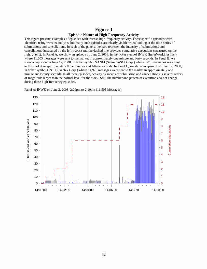
52

Figure 3 Episodic Nature of High-Frequency Activity

This figure presents examples of episodes with intense high-frequency activity. These specific episodes were

identified using wavelet analysis, but many such episodes are clearly visible when looking at the time-series of

submissions and cancellations. In each of the panels, the bars represent the intensity of submissions and

cancellations (measured on the left y-axis) and the dashed line provides cumulative executions (measured on the

right y-axis). In Panel A, we show an episode on June 2, 2008, in the ticker symbol INWK (InnerWorkings Inc.)

where 11,505 messages were sent to the market in approximately one minute and forty seconds. In Panel B, we

show an episode on June 17, 2008, in ticker symbol SANM (Sanmina-SCI Corp.) where 3,013 messages were sent

to the market in approximately three minutes and fifteen seconds. In Panel C, we show an episode on June 12, 2008,

in ticker symbol GNTX (Gentex Corp.) where 14,925 messages were sent to the market in approximately one

minute and twenty seconds. In all these episodes, activity by means of submission and cancellations is several orders

of magnitude larger than the normal level for the stock. Still, the number and pattern of executions do not change

during these high-frequency episodes.

Panel A: INWK on June 2, 2008, 2:00pm to 2:10pm (11,505 Messages)

Su

bm

issio

ns a

nd

ca

nce

lla

tio

ns

0

10

20

30

40

50

60

70

80

90

100

110

120

130

14:00:00 14:02:00 14:04:00 14:06:00 14:08:00 14:10:00

Cu

mu

lative

exe

cu

tio

ns

0

1

2

3

4

5

6

7

8

9

10

11

12

53

Panel B: SANM on June 17, 2008, 12:00pm to 12:10pm (3,013 Messages)

Panel C: GNTX on June 12, 2008, 12:00pm to 12:20pm (14,925 Messages)

Su

bm

issio

ns a

nd

ca

nce

lla

tio

ns

0

10

20

30

40

12:00:00 12:02:00 12:04:00 12:06:00 12:08:00 12:10:00

Cu

mu

lative

exe

cu

tio

ns

0

1

2

3

4

5

6

7

8

9

10

11

12

13

14

Su

bm

issio

ns a

nd

ca

nce

lla

tio

ns

0

100

200

300

12:10:00 12:12:00 12:14:00 12:16:00 12:18:00 12:20:00

Cu

mu

lative

exe

cu

tio

ns

0

10

20

30

40

54

Figure 4 Speed of Response to Market Events

This figure looks at the speed of responses to certain market events that have well-defined economic meaning. In Panel A, the market event is an improved quote

via the submission of a new limit order—either an increase in the best bid price or a decrease in the best ask price. Subsequent to this market event, we estimate

(separately) the hazard rates for three types of responses: (i) a limit order submission on the same side as the improvement (e.g., buy order submitted following

an improvement in the bid price), (ii) a cancellation of a standing limit order on the same side, and (iii) an execution against the improved quote (e.g., the best bid

price is executed by an incoming sell order). In Panel B, the market event is deterioration in the quote as a result of a cancellation of a standing limit order (e.g., a

limit buy order alone at the best bid price is cancelled and the best bid price therefore decreases). Subsequent to this market event, we estimate (separately) the

hazard rates for three types of responses: (i) a limit order submission on the same side as the quote deterioration, (ii) a cancellation of a standing limit order on

the same side, and (iii) an execution against the worsened quote. In all estimations, any event other than the one whose hazard rate is being estimated is taken as

an exogenous censoring event. The estimated hazard rate plotted at time t is the estimated average over the interval [t–1 ms, t). The hazard rate for a response can

be interpreted as the intensity of the response conditional on the elapsed time since the conditioning market event (e.g., the improved quote in Panel A).

Panel A: Responses to Quote Improvement

Ha

za

rd r

ate

(e

ven

ts p

er

se

co

nd

)

0.1

1.0

10.0

100.0

1000.0

Time since quote improvement (milliseconds)

0 10 20 30 40 50

Ha

za

rd r

ate

(e

ven

ts p

er

se

co

nd

)

0.1

1.0

10.0

100.0

1000.0

Time since quote improvement (milliseconds)

0 10 20 30 40 50

2007

Same-side submissionSame-side cancellationExecution against improved quote

2008

Same-side submissionSame-side cancellationExecution against improved quote

55

Panel B: Responses to Quote Deterioration Due to a Limit Order Cancellation

Hazard

rate

(eve

nts

per

second)

0.01

0.10

1.00

10.00

100.00

1000.00

Time since quote deteriorated by cancel (milliseconds)

0 10 20 30 40 50

Hazard

rate

(eve

nts

per

second)

0.01

0.10

1.00

10.00

100.00

1000.00

Time since quote deteriorated by cancel (milliseconds)

0 10 20 30 40 50

2007

Same-side submissionSame-side cancellationExecution against worsened quote

2008

Same-side submissionSame-side cancellationExecution against worsened quote