how to use demand systems to evaluate risky projects, with
TRANSCRIPT

Munich Personal RePEc Archive
How to use demand systems to evaluate
risky projects, with an application to
automobile production
Friberg, Richard and Huse, Cristian
Stockholm School of Economics, Stockholm School of Economics
2012
Online at https://mpra.ub.uni-muenchen.de/48906/
MPRA Paper No. 48906, posted 16 Feb 2014 01:18 UTC

1
How to use demand systems to evaluate risky projects, with an
application to automobile production
Richard Friberg, Stockholm School of Economics and CEPR
Cristian Huse, Stockholm School of Economics
This version: December 5, 2012
Abstract
This article introduces a method to quantify the effect of a firm’s strategic choices on the risk profile
of its profits at different horizons. We combine a demand system for differentiated products with
counterfactual paths of risk factors. Prices, costs and quantities respond endogenously to the
counterfactual state of the world. The draws on risk factors are generated using copulas, in a way that
flexibly can be adapted to the risks faced in various industries. We illustrate the method by studying
how the US operations of German carmakers BMW and Porsche are affected by the decision to
relocate production, i.e. operational hedging. We find that for plausible costs of building a plant,
production in the US is attractive for BMW, but not for Porsche.
JEL Classification Codes: F23, L16, L62
Keywords: Exchange rate exposure, macroeconomic exposure, operational hedging, natural hedging,
risk management.
We are grateful to the Swedish Research Council (VR) and Jan Wallanders and Tom Hedelius Stiftelse for financial support. We thank Elisa Alonso, Marcus Asplund, Johannes van Biesebroeck, Carlos Noton, Rickard Sandberg and seminar audiences at CEMFI, the CEPR/JIE workshop in Applied IO in Tel Aviv, EARIE in Istanbul, ESSEC, Foro de Finanzas in Elche, HECER, Lund, Stockholm School of Economics, Uppsala and Queen Mary for valuable comments. Email: [email protected]. Correspondence address: Stockholm School of Economics, Dept of Economics, Box 6501, SE-113 83 Stockholm, Sweden. Email: [email protected]. Correspondence address: Stockholm School of Economics, Dept of Finance, Box 6501, SE-113 83 Stockholm, Sweden.

2
Introduction
The future profits of a firm depend on the realized values of risk factors that affect its costs and
demand. Profits also depend on the strategic choices made by the firm itself and by its competitors.
Furthermore, the strategic choices and the risk factors interact in possibly complex ways: locating
production abroad or repositioning a brand to a premium segment will, for instance, alter the way that
an exchange rate change affects costs and the profit maximizing price.
How can a manager contemplating different strategic choices gauge the effect of those choices
on the risk profile of profits? This is the motivating question of this paper. Our methodological
contribution is to show how to combine a demand system and risk factors to evaluate strategic choices
at different horizons. Examples of strategic choices that we have in mind concern the scale of
operations, production locations, product line length and brand positioning. Our starting point is that if
we want to examine firm profits under different choices, in different states of the world, we desire a
fully worked out structural model that relates demand to prices and to strategic choices. In recent
years, following Berry, Levinsohn and Pakes (1995, BLP hereafter), structural models of demand have
been developed in the field of Industrial Organization. These models have, with one exception, not
been applied to the study of risk and typically consider only one or a few counterfactual scenarios.
Thus, models of demand similar to the one we use have been applied to evaluate mergers (Nevo
(2000)), to measure the impact of trade policy (Berry, Levinsohn and Pakes (1999)), to quantify the
welfare effects of entry (Petrin (2002)) and to address the sources of the declining market share of US
auto manufacturers in Train and Winston (2007). These demand estimation methods have also been
applied to marketing-related issues, see Chintagunta and Nair (2011) for an overview. Perhaps closest
in spirit to us is Berry and Jia (2010), who provide an ex post analysis of the sources of profit changes
in the US airline industry, using a model of demand similar to the one we propose to use in a forward
looking manner.
Demand estimation techniques are one building block for the method we propose. Our other
building block is a framework to generate counterfactual draws on the risk factors. Examples of risk
factors that we envision are input prices, exchange rates and economy-wide shocks to demand. The
estimations that are used to generate the counterfactual draws of the risk factors are separate from the
demand modeling. This allows one to for instance use long time series of macroeconomic variables
while only using shorter time series data for the product market. We use copulas to provide a flexible
way of modeling the correlation of the draws of the risk factors (see Patton (2009) for an overview of
the use of copulas in Finance or Danaher and Smith (2011) for applications in marketing). The final
step in our methodology is to feed the random draws on risk factors into the demand system, letting all
prices, costs and quantities respond to generate counterfactual distributions for cash flows. Comparing
such distributions for different strategic choices, and their net present value, brings us to our goal.

3
While neither demand estimation nor modeling of risk factors is novel we hope to show that
combining these tools in the way that we propose is a fruitful way of analyzing strategic choices for a
firm. While our aim is to contribute to methodology, we illustrate how the methods can be applied by
focusing on production location choices of German carmakers BMW and Porsche. German carmakers
that have substantial sales in the US are exposed to changes in the exchange rate between the euro and
the US dollar. One response from several carmakers has been to open up production facilities in the
US. For instance, BMW produces a number of models in the US and states in its 2007 annual report (p
62) that “From a strategic point of view, i.e. in the medium and long term, the BMW Group endeavors
to manage foreign exchange risks by ‘natural hedging’, in other words by increasing the volume of
purchases denominated in foreign currency or increasing the volume of local production.”1 Other
carmakers have followed different strategies: despite obtaining 30-40 percent of its sales in North
America, Porsche produces exclusively in the euro area. We quantify how the risk profiles of
Porsche’s and BMW’s US sales depend on the production location.2 We use data on prices, quantities
and product characteristics for the top segments of the US auto market for 1995-2006 to estimate
demand that serves as the main input in our counterfactuals. The data are at the national level and
products are defined at the model line level (such as Porsche 911, Ford Explorer and so forth). We
consider three risk factors: Two real exchange rates and a measure of the business cycle. To estimate
the stochastic properties of the risk factors we rely on data from 1973 onwards.
In terms of methodology we relate to two broad literatures apart from the ones already
mentioned. The first literature is rooted in Corporate Finance and Management where it has long been
taught that a way to evaluate investment projects with risky cash flows is to consider profits under the
different realizations of risk factors and weigh these realizations according to their likelihood. One
selects a probability distribution for each of a set of variables that affect profits, such as price and
market size, and then use these distributions to generate counterfactual profit distributions (see Hertz
(1964) for an early proposition and textbook coverage in Brealey and Myers (2003), Mansfield et al
(2009) or Damodaran (2010)). The method we propose applies the same logic but, by using a demand
system, we circumvent several of the troublesome features of the approach that is associated with the
literature since Hertz. Using structural estimates of demand allows us to deal with the fact that cash
flows themselves are likely to be endogenous to the investment project under consideration in a
straightforward manner. It also, in an economically sound way, introduces the correlation between
endogenous variables such as quantities, costs and prices – of both the firm itself and its competitors.
1 The German carmaker Volkswagen also opened a US plant in 2011 and states in its annual report 2009 (p 188) that “Foreign currency risk is reduced primarily through natural hedging, i.e. by flexibly adapting our production capacity at our locations around the world, establishing new production facilities in the most important currency regions and also procuring a large percentage of components locally.” 2 Indeed, Porsche is enough of a schoolbook case on exchange rate exposure that it is featured as mini cases in two of the leading textbooks in international finance (Eiteman, Stonehill and Moffett (2007, p 322) and Eun and Resnick (2007, p 236)) and a popular business school case: Porsche exposed (Moffet and Petitt (2004)).

4
Furthermore, rather than conjecturing probability distributions about variables such as sales (for which
we often have short relevant time-series data) we can use longer time series to estimate probability
distributions for many cost and demand shifters such as prices of raw materials and exchange rates.
The discipline imposed by this should be especially valuable given the extensive evidence that humans
are prone to behavioral biases when probabilities are involved (see for instance the seminal work of
Tversky and Kahneman (1971) and the large literature that has followed).
The second literature that we relate to develops tools to estimate dynamic oligopoly games
(see for instance Ericson and Pakes (1995), Bajari, Benkard, Levin (2007) or Ackerberg et al (2006)
and Aguirregabaria and Nevo (2012) for surveys). These papers are closely related to the present paper
in that they develop tools to estimate structural models of demand and use them to examine industries
over time, while allowing for strategic choices to affect the payoffs of competitors. However, when
considering many strategies of several competitors the state space grows rapidly and computational
costs are an important restriction. At the risk of oversimplifying, the papers in this literature have
largely concentrated on inferring parameters or behavior that is hard to observe directly, such as the
sunk costs of entry. Such information is of clear importance to a policymaker trying to for instance
gauge the probability of entry following some policy change (for steps in the latter direction see
Benkard, Bodoh-Creed and Lazarev (2010)). The assumptions on the type of shocks faced by firms are
typically quite stylized (such as i.i.d. firm specific shocks to the sell-off value of the firm) and neither
the time series properties of shocks, nor using the models in a forward looking manner, have been the
focus of this literature. In contrast, the present paper puts the future distribution of shocks center stage
– that is, it focuses on how should you value the profits associated with an investment when
exogenous risks such as exchange rates or the business cycle are important. For many applications we
ultimately wish to have a framework that is suited for both dealing with uncertainty that arises because
of the strategic interaction and for dealing with the risks that stems from the stochastic nature of
exogenous demand and cost shocks – see Besanko et al (2010) for such a combination in a stylized
framework. For the time being we believe that is useful to complement work that focuses on the
strategic interaction with work that focuses on how exogenous shocks feed through into profits – and
how the impact of cost and demand shocks depends on strategic choices. The relation between the
present work and research in finance and operations management is perhaps easier to appreciate after
we have covered the model, and the penultimate section of the paper therefore spells out how our
research informs research in these other fields.
In the next section we present the methodology for generating counterfactual draws on cost
and demand shocks and for estimating demand and counterfactual profits. In Section 3 we present our
empirical application and in Section 4 we show the results from demand estimation and from the
generation of counterfactual macroeconomic conditions. The counterfactual profits are then presented
5
and analyzed in Section 5. We discuss further relation to the previous literature in Section 6 and
conclude in Section 7.
2 How we generate counterfactual distributions of discounted cash flows.
Overview
The ultimate object of interest in our application is the probability distribution of profits, translated
into euros, stemming from the US sales for BMW and Porsche. By producing a model locally in the
US rather than in the euro area, the risk profile will be affected. We consider three risk factors: The
real exchange rates between the dollar and the euro (usd/eur), between the dollar and the Japanese yen
(usd/jpy) and the measure of consumer confidence published by the Conference Board. Consumer
confidence is frequently mentioned in the industry as an important covariate for the demand for cars,
as stressed by Ludvigson (2004). To estimate demand we use data on the products of BMW and
Porsche, as well as of the products with which they compete.
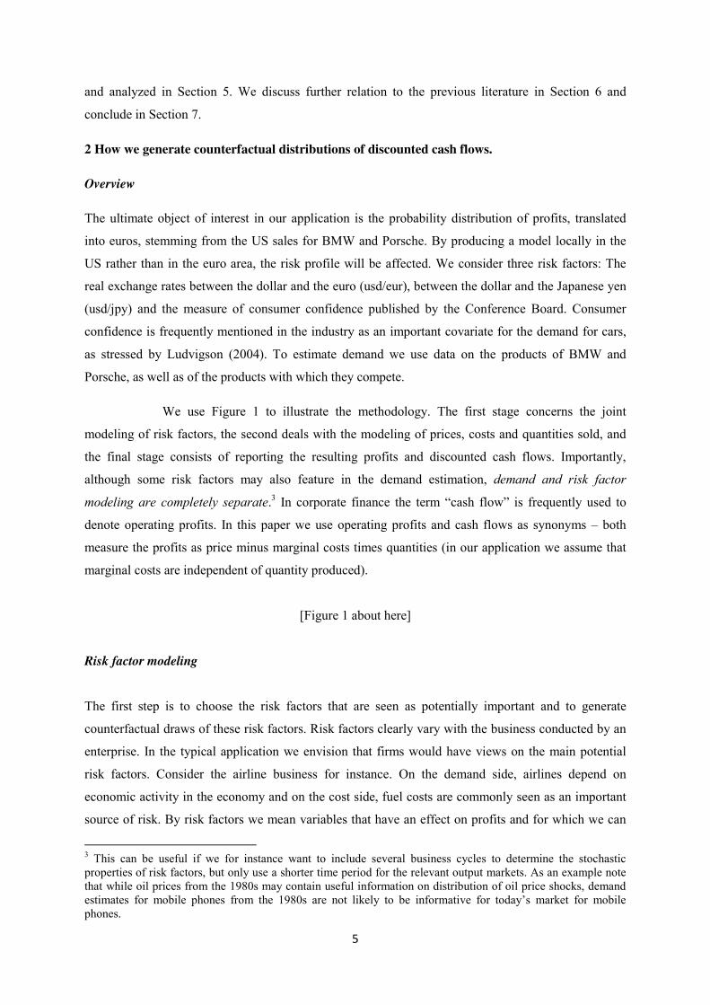
We use Figure 1 to illustrate the methodology. The first stage concerns the joint
modeling of risk factors, the second deals with the modeling of prices, costs and quantities sold, and
the final stage consists of reporting the resulting profits and discounted cash flows. Importantly,
although some risk factors may also feature in the demand estimation, demand and risk factor
modeling are completely separate.3 In corporate finance the term “cash flow” is frequently used to
denote operating profits. In this paper we use operating profits and cash flows as synonyms – both
measure the profits as price minus marginal costs times quantities (in our application we assume that
marginal costs are independent of quantity produced).
[Figure 1 about here]
Risk factor modeling
The first step is to choose the risk factors that are seen as potentially important and to generate
counterfactual draws of these risk factors. Risk factors clearly vary with the business conducted by an
enterprise. In the typical application we envision that firms would have views on the main potential
risk factors. Consider the airline business for instance. On the demand side, airlines depend on
economic activity in the economy and on the cost side, fuel costs are commonly seen as an important
source of risk. By risk factors we mean variables that have an effect on profits and for which we can
3 This can be useful if we for instance want to include several business cycles to determine the stochastic properties of risk factors, but only use a shorter time period for the relevant output markets. As an example note that while oil prices from the 1980s may contain useful information on distribution of oil price shocks, demand estimates for mobile phones from the 1980s are not likely to be informative for today’s market for mobile phones.

6
estimate a probability distribution. Risk factors in our setting can thus for instance be market prices
(such as exchange rates or prices of raw materials) or demand shocks (for instance captured by
business cycle measures).
There are a number of ways one generate counterfactual draws on the risk factors. Intuitively,
the idea is to capture the main features of the joint distribution of the risk factors and generate random
draws based on it. Jointly modeling the factors, instead of assuming their independence, is important
in a number of applications - for instance, in the hypothetical case where costs are subject to exchange
rates and demand is subject to interest rate risk, the cost and demand risk factors are likely to be
correlated. One could assume factors follow a parametric distribution. Alternatively, one could
estimate a vector autoregressive model of factor returns.
In this paper we make use of copula methods. In recent years copulas have been used to
model the interdependencies between asset prices (see for instance Jondeau and Rockinger (2006),
Kole et al (2007)). The attractiveness of the copula approach is that it allows modeling of the
univariate processes separately from their dependence. The core result with regard to copulas is due to
Sklar (1959) who showed that any joint distribution of random variables can be decomposed into two
parts: The marginal univariate distributions and a function, the copula function, which captures the
dependency between the marginals. Consider three random variables X1, X2, X3. The joint cumulative
density function (cdf) is given by H(x1, x2, x3)=Pr[X1≤ x1, X2≤ x2, X3≤ x3]. For each Xi, i=1,2,3, the
marginal cdf is given by Fi(xi)=Pr[Xi≤ xi]. Using C to denote the copula function we can thus write
H(x1, x2, x3)=C(F1(x1), F2( x2), F3( x3)).
As detailed in Section 4.3, we model the marginal distributions for exchange rates and consumer
confidence using GARCH processes. Our first step is thus to estimate the parameters from univariate
GARCH processes and then estimating the copula relation between the residuals. We then use these
estimated parameters to generate 200 random shocks for each future period in the forecast horizon and
let the shocks in each period follow the GARCH and copula relations. We use counterfactual values
12, 24, 36 and 48 months ahead from the end date July 2006.
In general terms, the first step is thus the modeling of the joint distribution G(.) of risk
factors (f1,…,fK). We denote one given set of simulated draws by f[s],t+n, where s=1,...,S is the
simulation draw and t+n denotes that the draw refers to n periods ahead.
Model
Figure 1 also illustrates how risk factors f[s],t+n feed into costs, prices and quantities sold in the general
case. To estimate the relation between the risk factors and demand one could in principle estimate
product level demand curves – regressing quantities on prices of the own product, the prices of

7
competitors and demand shifters represented by (some of) the risk factors. A concern in many
differentiated product industries is that product attributes and the set of competitors change over time
which implies that we need to identify effects from short time series. Such problems are commonly
faced in estimating demand for differentiated products and are the motivation for the estimation
approach that we describe here.
We follow BLP (1995) who estimate a random-coefficients (RC) logit model for automobiles
in the US market. We do not develop every detail of the model, but rather refer to previous treatments
including, in particular, BLP (1995) and Berry (1994); Davis and Garcés (2010) provide an accessible
discussion. The demand system builds on discrete choice modeling of individual choices, but only
market level data are needed. The key assumption, that allows us to avoid directly estimating an
infeasible number of cross-price elasticities, is that we model demand as dependent on product
characteristics. Thus, when for instance buying a car in the BMW 3-series, the consumer purchases a
combination of observable product characteristics. In our application to car demand we use price, size,
horsepower/weight, brand and country of production. Any risk factors that affect demand should also
be included in the specification. In our case, as already mentioned, we include consumer confidence as
a measure of the state of the world which affects the utility of buying a car. By imposing a structural
model of demand, the own- and cross price effects are found by using the estimated coefficients of the
model in combination with the model structure. Modeling demand as dependent on characteristics also
allows us to handle changing product characteristics and product introductions. Define the conditional
utility for individual i when consuming product j from market m (where m can refer to both the time
and geographical dimension) as:
where xjmk are observed product characteristics and ξjm represent unobserved (by the econometrician)
product characteristics but that are assumed to be observed by all consumers. Different consumers are
allowed to have different valuation of the various characteristics. Following the literature, we
decompose the individual coefficients
where βk is common across individuals, vki is an individual-specific random determinant of the taste for
characteristic k, which we assume to be Normally distributed and σk measures the impact of v on
characteristic k. Finally, εijmt is an individual and option-specific idiosyncratic component of
uijm ∑k1
K
x jmkik jm ijm , i 1, . . . , I; j 1, . . . ,J; m 1, . . . ,M
ik k kv ki

8
preferences, assumed to be a mean zero Type I Extreme Value random variable independent from both
the consumer attributes and the product characteristics. The specification of the demand system is
completed with the introduction of an outside good with conditional indirect utility ui0=0m+0+i+i0,
since some consumers decide not to buy any car.
Risk factors may also have a direct impact on the cost of production. We focus on marginal
costs and follow BLP (1995) and others in this literature and assume that marginal costs are constant.
In our case the exchange rates affect the marginal cost of car production in the euro area and in Japan
relative to the US market, and we can view exchange rates as marginal cost shifters. Via the effect on
prices, this marginal cost shock will feed through into demand as well. If a firm were to use these
methods to evaluate projects, it would use own internal calculations to model the link between costs
and input prices or other cost shocks such as exchange rates. We lack this detailed data and therefore
make an assumption of Bertrand competition by multi-product firms to back out the marginal costs
that are implied by this form of competition when coupled with the demand specification that we use.
This is the way that marginal costs have typically been estimated in the previous literature that applies
these demand estimation methods.
Demand will also depend on prices, which will endogenously depend on the
realizations of the risk factors. If used by the firm itself, with knowledge of internal costs and pricing
rules, it can operationalize these pricing rules in the simulations. If the firm applies a fixed markup on
costs for instance, the relation between price and costs will be given by this relation in the
counterfactual simulations. To model prices of competing products under different scenarios the firm
may also use historical data, and regress prices on realizations of risk factors and product fixed effects.
Using the point estimates from such hedonic regressions, it is then straightforward to use the estimated
coefficients to generate counterfactual prices that reflect the draws of the risk factors in each
counterfactual scenario. Alternatively, one can use an assumption of all firms setting prices in a static
Nash-Bertrand fashion. Note however while the type of models that we build on are generally seen as
giving a plausible representation of substitution patterns on the part of consumers, static Nash-
Bertrand pricing may overestimate the degree of price adjustment in many cases. In her study of the
US car market, using similar tools as we do, Goldberg (1995, p. 937) for instance notes that “After
1985, the model predicts a significant increase in German import prices as a consequence of a
dramatic dollar depreciation which is not matched by the data. In fact, the prices of German imports
remained fairly constant during 1986 and 1987.” That consumer prices are stable by assumption, but
quantities vary over the business cycle is a central feature in much of macroeconomic modeling for
instance.4 Nakamura and Zeron (2010) and Goldberg and Hellerstein (2012) introduce dynamic price
4 See Okun (1981) for a seminal reference. Copeland and Hall (2011) use transaction prices for the big three US
carmakers and show that demand shocks have a small impact on price and are absorbed almost entirely by sales and production decisions.

9
adjustment in a framework similar to ours. Including dynamic price adjustment with a large number of
counterfactual demand and cost shocks would be very computationally demanding and we therefore
opted for hedonic price regressions to yield counterfactual prices in a straightforward manner.5
Outcome
We have thus outlined how the random draws of the risk factors can be modeled to affect prices, costs
and demand. The final outcome of a set of n-period-ahead simulation draws f[s],t+n is the profit function
[s],t+n. By repeating this iteration S times one can approximate the distribution function of the profits
of firm with their empirical counterpart. It is worth emphasizing again that the empirical distribution
of profits is also conditional on a strategy, e.g. having the entire production chain located in the home
market as opposed to consumer market, or stabilizing prices in the currency of the market rather than
passing through costs. Discounting future cash flows under the different scenarios allows comparing
the outcomes of different strategies. We can discount future cash flows along each of the simulated
paths of the risk factors. Therefore we can use the framework not only to examine expected profits but
also consider differences in the tails of the profit distribution, which may be of central interest for risk
management purposes and for evaluating the effect of different strategic choices on the risk profile of
a firm.
For each set of draws of exchange rates and consumer confidence we generate
operating profits at the product level for all firms, but given our focus will report them only for BMW
and Porsche. At the producer level, total cash flows from US sales equal the sum of cash flows from
all products controlled by the firm in question and translated into the home currency. Cash flows for a
product that is produced in the euro area by a firm based in the euro area at period t+n, for a set of
counterfactual draws s, is therefore given by
, = , ̂ , − ̂ , , , , ̂ , ( ) . (1)
The eur/usd exchange rate here is one draw from a counterfactual distribution. The price ̂ reflects the
counterfactual vector of draws of exchange rates. Counterfactual demand, , depends on the vector of
counterfactual prices for all producers ̂, and on the counterfactual realization of , the consumer
confidence. The marginal cost ̂ is assumed to be independent of volume and fixed in the currency of
the production location. The last period for which we estimate demand is model year 2005-2006 and
we simulate counterfactual predictions looking ahead from this date. In the case where production of a
model is in the euro area, we take this marginal cost for each car model to be fixed in euros in the
forward looking scenarios. Similarly, marginal costs of cars produced in other currency areas are
5 Our motivation here is somewhat related to the estimation of policy functions that form the first stage in Bajari, Benkard and Levin (2007).

10
assumed to be fixed in the currency of production location. As quantities vary in the simulations total
costs will vary across the simulation draws. Furthermore, the marginal costs of cars produced outside
the US will shift, when expressed in US dollars, reflecting the draws from the exchange rate
distributions.
For a BMW or Porsche model that is counterfactually produced in the US we assume
that the marginal cost, in US dollars, is fixed at its 2006 level. Assuming marginal costs fixed in either
the home or the market currency is a simple way to capture two polar cases regarding the correlation
between exchange rates and marginal costs. In using the backed out marginal costs from 2006 the
counterfactual simulations for BMW and Porsche start from a situation where marginal costs are equal
in EU and US. We thus tone down any level differences in costs as a motivation for producing abroad,
which we would argue is a reasonable simplification in this case. For BMW and Porsche we compare
production in Germany with production in the US. Average differences in factor prices are limited
between these two countries. For instance, over 1992 to 2005 wages in manufacturing are on average
6.8 percent higher in US than in Germany.6 The swings in exchange rates are, for these production
locations and a given technology, likely to overwhelm level differences in production costs. For
example, the usd/eur exchange rate fell from 1.4 in 1996-7 to 0.88 in 2001-2 and then rose again to
1.22 by 2005-6. Inflation is low in both countries during this time so such changes translate into cost
differences of production. Like most of the literature that applies these kind of demand models (such
as BLP) we do not have access to detailed marginal cost information – we therefore opted for these
simple and transparent assumptions on marginal costs rather than ad-hoc assumptions about for
instance supplier networks in Germany and US affect marginal costs. As we use the empirical exercise
as an example meant to illustrate how the methodology can be used – and the ultimate goal is to
provide a tool that will be useful to decision makers in firms (or consultants with access to firm level
data) rather than competition authorities we do not believe that this is not an important weakness.
Alternative assumptions on marginal costs are straightforward to implement, should one wish to do so.
If a producer located in the euro area (EU) instead produces a model locally in the US,
the cash flow from that model is
, = , ̂ , − ̂ , , , , ̂ , ( ) . (2)
When production is in the EU, as in equation (1), costs are thus stable in euro whereas the exchange
rate has a large effect on revenue. In contrast, in (2) costs and revenue are in the same currency and it
is only the net profit that is affected by the exchange rate.
6 Source: OECD, labor compensation per employee in manufacturing, expressed in USD using PPP-adjusted exchange rates.

11
To produce cars targeted to the US market locally in the US can be seen as operational
hedging. An alternative for a risk-averse owner is to use financial hedging and we note that a possible
application for a manager is to also include cash flows from various financial hedges at this stage of
the simulations.
To calculate the net present value (NPV) of the different production locations we need three
ingredients: A set of future profits as outlined above, an appropriate discount rate, and initial outlays.
We do not aim to make a methodological contribution on how to establish the appropriate discount
factor.7 We therefore use standard assumptions from corporate finance and discount cash flows using
the weighted average cost of capital (WACC). We take the profit distribution 4 years ahead as
reflecting the long run distribution in the calculation of NPV. We thus calculate the NPV of each of
the 200 streams of cash flows. As initial outlays we take back-of-the-envelope calculations of the cost
of establishing a new production facility.
3 The empirical application
Data
We use quantity sold, recommended dealer price and product characteristics for all cars sold in the
luxury, sport, SUV (sports utility vehicles) and CUV (cross over utility vehicles) segments in the US.
The main source of data is WARDS who supplied us with a panel of monthly sales by model line
(BMW 3 series, Porsche 911 etc). We examine the period from August 1995 to July 2006. In our
regression analysis we aggregate sales to 12-month periods, but rather than use calendar years we note
that new models, and a new recommended dealer price, appear in late summer each year. 8 Our time
unit of analysis therefore runs from August to July the following year and we use the term model-year.
In Table 1 below we show some descriptive statistics for our set of cars. We examine
the upper segments of the car market and the mean real price is roughly stable at 35 000 dollars. The
lowest price is for a Pontiac G5 and the highest is for a Porsche Carrera GT. On average some 30 000
to 40 000 cars are sold per model in a given model-year. The largest selling name plate in the data is
the Ford Explorer. The number of models in the data increases substantially over the period, mainly
reflecting growth in the CUV and SUV segments.
[Table 1 about here]
7 See Cochrane (2011) for an overview of current research on discount rates. 8 We use the recommended dealer price as our measure of price -- a simplification that we share with previous
work examining the car market at this level. In practice dealers buy from the manufacturer and rebates on the car are given, either in the form of lower prices, discounted financing or buy-in's of the customers' old car: see Busse, Silva-Risso and Zettelmayer (2006) for an analysis of pricing at a sample of Californian retailers.

12
The dollar appreciated against the euro and yen up until the middle of the period, after
that it depreciated against the euro but remained rather stable against the yen. The consumer
confidence measure of the business cycle shows substantial variability as well.
The US market for BMW and Porsche
German-based BMW is one of the ten largest car manufacturers in the world. Over the period, on
average, 23.7 percent of BMW deliveries of cars are in North America.9 Compared to other auto
manufacturers the accounting figures point to BMW as a profitable firm with high margins: its’ return
on assets is on average 5.3 percent and the profit margin is 15.6 percent (EBITDA operating margin
before interest, taxes, depreciation and amortization).10 The main products for BMW over this period
are the luxury cars in the 3, 5 and 7 series. At the start of the period it also sells the luxury sports car
Z3. BMW further controlled the Land Rover and Range Rover lines that were produced in the UK. In
2000 Ford Motor Company took control of these brands. Since 1999 BMW has production capacity in
a US factory in Spartanburg. In 2005-2006 the luxury sports car Z4, as well X3 and X5, that are
classified as middle luxury CUVs are produced in this plant. All other products are produced in the
euro area, apart from the Mini, which is produced in the UK. We therefore expect a potentially
important role for the usd/euro exchange rate on BMW profits. Indeed the annual report for 2005 (p.
56) notes that “Of all the currencies in which the BMW group does business, the US dollar represents
the main single source of risk; fluctuations in the value of the US dollar have a major impact on
reported revenues and earnings.”
Turning now to Porsche, the North American market accounted for an average of 35 percent
of its sales revenue. During this period all production of Porsche cars is located in Europe. During the
time period that we examine, accounting profitability and operating margins are high at Porsche: the
return on assets is on average 19.7 percent and the operating margin is 24.7 percent. Porsche's main
product over the period is the 911 - a name plate that was introduced in 1963 and still accounts for
almost half of Porsche’s US revenues at the end of the sample period. At the start the 911 is the only
model marketed by Porsche in the US. The small roadster Boxster is then introduced in late 1996. The
Cayenne is introduced in 2003 (identified as a middle luxury CUV by WARDS) and the sports car
Cayman in 2005. In 2004 Porsche adds the top of the line sports car Carrera GT. After only having
had assembly in Germany, Porsche starts production of its Boxster in Finland in 1997 (under an
agreement with Finnish producer Valmet). Since 2005 also the Cayman model is produced in Finland
which, like Germany, is part of the euro zone.
9 Source. BMW Annual reports 2005 and 2000. 10 Average over August 1999 to July 2006. Corresponding return on assets for Daimler (1.5%), Ford (-0.4%), Toyota (6.8%) and Volkswagen (2.4%). Corresponding EBIDTA margins for Daimler (8.1%), Ford (6.8%), Toyota (13.9%) and Volkswagen (10.5%). Source for this and the statistics that follow for Porsche: Orbis.

13
4. The estimated model
4.1 Demand Estimates
Table 2 reports estimates of two RC logit specifications for the US car market. Both use price, engine
power (HP), size and whether non-manual transmission is included in the baseline model as
observable product characteristics. We model price as a random coefficient with a mean effect of price
on utility and individuals’ coefficients on price follow a distribution as outlined in Section 2. Both
specifications also include time (model-year), country of origin, and brand fixed-effects. We treat
price as endogenous in our demand specification. To estimate our model, besides the exogenous
characteristics, we use the BLP instruments (following BLP (1995)), a set of polynomial basis
functions of exogenous variables exploiting the three-way panel structure of the data, consisting of the
number of firms operating in the market, the number of other products of the same firm and the sum of
characteristics of products produced by rival firms. As documented in the literature (Berry 1994, BLP
1995), not accounting for the endogeneity of prices results in an attenuation bias, that is, the price
coefficient is biased towards zero, and this is what our findings also suggest: the uninstrumented
version of Specification I has a price coefficient of -0.002, well below the instrumented ones at -0.021.
Besides the tenfold increase in the slope of the demand curve, at 27.52 (and significant at the one
percent level), the F-statistic of the first-stage regression of price on the exogenous regressors is well
above the rule-of-thumb value of 10 suggested by Staiger and Stock (1997). This suggests that
instruments are not weak and that there is no evidence that the instrumented price coefficient is biased
towards the uninstrumented one. Instruments are also not rejected when computing tests of
overidentifying restrictions, as reported in Table 2.
[Table 2 about here]
The stance in which Specifications I and II differ is in the treatment of consumer confidence and
market segment variables. Specification I uses consumer confidence and separate fixed-effects for
market segments. In contrast, Specification II uses interactions of market segments and consumer
confidence. Specification II thus allows asymmetric responses in market shares according to the
market segment a model belongs to, according to which economic outlook consumers expect to
prevail. Both specifications have significant coefficients for the mean and for the dispersion of price
coefficients, whereas the remaining characteristics are usually not significant. In fact, most of the
explanatory power for market shares tends to come from brand and market segment fixed-effects.
The (own) price elasticities (equivalently, markups) of the models in Specification II
are in the range 3.7-7.3 with an average elasticity 6.0, thus broadly in line with previous studies of the
car industry, notably Petrin’s (2002) RC logit estimates using micro data (see, for instance, column 6

14
of his Table 9).11 Interestingly, the estimates for Specification II suggest an intuitive "pecking order"
effect of the interaction terms. For instance, demand for the "Upper Luxury" segment tends to be more
sensitive to consumer confidence than that of the "Middle Luxury" segment, which in turn is more
sensitive than that of the "Lower Luxury" segment. We interpret these results as evidence that,
conditional on buying a car, consumers are more likely to purchase models from high-end segments
the more confident they are about the economic outlook.
4.2 Price setting
Demand will depend on prices, which will endogenously depend on the realizations of the risk factors.
When faced with the task of estimating prices of a new equilibrium, e.g. following a merger between
two firms, economists typically assume a form of conduct, say Bertrand-Nash, and compute the new
equilibrium following the change in product ownership due to the merger. Recently, Nakamura and
Zeron (2010) and Goldberg and Hellerstein (2012) introduce dynamic price adjustment to account for
pass-through in a framework similar to ours. While increases in computing speed may make this the
preferred scenario in future work, we have instead opted for hedonic price regressions as a
straightforward way to generate empirically plausible counterfactual prices (since we perform
equilibrium calculations based on joint realizations for a high number simulations in order to
approximate the empirical distribution of firm profits under each scenario). For managerial
applications we see this as an attractive solution awaiting further improvements in computing speed.
We use the coefficients from hedonic regressions to generate counterfactual prices. We regress
real prices on forward exchange rates interacted with country of origin, product characteristics (HP,
size, transmission) and product fixed effects. To gauge if the results are reasonable we report the
elasticities in Table 3. The exchange rate pass-through in this regression is 0.146 for the euro exchange
rate and 0.116 for the Yen.12 Both are significant at the 5 percent level. Comparing to other estimates,
they are somewhat on the low side. A number of studies examine pass-through in import prices (see
Goldberg and Knetter (1997) for an early survey) and find pass-through elasticities that are frequently
equal to about one half. Note however that pass-through at the border is typically substantially higher
than measured pass-through at the retail level. We can also compare to another non-structural estimate
for the US auto market, Hellerstein and Villas-Boas (2010). The 24 models in their study exhibit an
average pass-through of exchange rates into transaction prices of around 38 percent, but with large
standard deviations.
[Table 3 about here]
11 Goldberg (1995) finds elasticities in the range 1.1-6.2 across specifications and market segments, using data from 1983-1987. 12 The elasticity with respect to horsepower is 0.166 and significant at the 1 percent level. Size and transmission are not significant, but the car model fixed-effects capture much of the variation that could identify these elasticities; the adjusted R-square for this regression is 0.986.

15
4.3 Counterfactual shocks
We use bimonthly data for consumer confidence and the real exchange rates for the period January
1973 to July 2006 to estimate the statistical properties of these variables, which we then use to
generate our counterfactual draws. We use a multivariate t-copula to model the dependence between
our three stochastic variables of interest. Define ( ) ≡ . The t-copula is then defined by ( , , ; , ) = , ( ), ( ), ( )
where Tυ,ρ is the cdf of the multivariate Student’s t-distribution with correlation matrix ρ and degrees
of freedom υ. The cdf of the univariate student’s t-distribution with υ degrees of freedom is denoted by
tυ. An attractive feature of the t-copula is that it allows for a higher dependence between extreme
events than for instance the Gaussian copula.
We use GARCH(1,l) models to estimate the exchange rate processes. Use yit to denote
the logarithmic returns (first-differences of logarithmic series) in the real usd/eur and real usd/jpy
respectively between time t and t-1. We assume that the process followed by yit is given by = + = + + . That is, today’s realization is equal to the last period’s value plus a possible drift term and a random
shock. The error term η is assumed to follow a t-distribution with mean zero. We allow the shocks to
have time varying volatility.
We model the process followed by consumer confidence in first differences, such that
yit is the difference in consumer confidence between time t and t-1:13
= +
The decreases in consumer confidence are greater than increases. To capture this asymmetry we model
the shocks using an exponential GARCH model, EGARCH(1,1). Again, let the error term η follow a t-
distribution with mean zero and define z=η/. Following Nelson (1991) we then assume that volatility
can be modeled as ln = + ln( ) + + (| | − | |). 13 As opposed to exchange rates, consumer confidence is not a traded asset. Moreover, anecdotal evidence suggests that individuals and firms focus on the levels and, more importantly, at the changes of this factor, thus the use of first differences in this case.

16
If is negative, the conditional volatility will be greater for negative shocks than for positive shocks.
We fit a Student's t-copula to the residuals that we estimate by the GARCH and EGARCH processes.
The estimation output for the marginal distributions is given in Table 4. The significant coefficient on
lagged volatility in the usd/eur relation points to that volatility is indeed time-varying at this
frequency. The process for consumer confidence reflects a pattern where the typical change is an
upward drift but that negative shocks are associated with greater volatility (captured by the negative
coefficient on the leverage term).
[Table 4 about here]
The degrees of freedom for the t-copula are estimated to be 21.65. The estimated correlation
coefficients using the t-copula are -0.085 between usd/eur and consumer confidence, 0.063 between
usd/jpy and consumer confidence and 0.522 between usd/eur and usd/jpy. Combining these estimates
allows us to generate counterfactual shocks where the marginal distributions follow the GARCH
processes and the co-dependence follows a t-copula in each period. Adding the succession of these
shocks to the starting values in July 2006 then gives us counterfactual paths of the exchange rates and
consumer confidence. As an example of our results, Figure 2 shows the distributions for counterfactual
draws for these three variables 12 months ahead from July 2006. The histograms show the densities
for the respective variable and the scatter plots the relation for each bilateral comparison. The scatter
plot in the lower left hand corner for instance plots counterfactual draws of usd/eur against
counterfactual draws of usd/jpy.
[Figure 2 about here]
As seen, the draws reflect substantial dispersion for all three variables. The skewness of
consumer confidence is visible. The starting value in July 2006 is 134 and we see predictions for 12
months ahead centered at this level (median across the draws is 146, mean 139) but a long tail of
weaker realizations. As seen in the scatter plots in the middle row, the relation between consumer
confidence and the exchange rates is weak. The positive relation between the two exchange rates on
the other hand is clearly visible in the scatter plots in the upper right and lower left corner. These then
are the counterfactual levels of macro variables that are fed into the demand system when we consider
the 12 month horizon ahead. Note that by the additive nature of the shocks we can view our results as
simulating 200 possible paths of the underlying variables. As we expand the forecast horizon some of
the paths for consumer confidence are predicted to be too low, or even negative. In these cases we
replace the value with a hypothesized lower threshold of 10. The lowest level in the time period
covered by our data is 15.8 (December 1982).
5. Simulation Results

17
We now turn to a presentation of the simulation results, feeding the counterfactual shocks into demand
and costs and letting all prices respond. We compare different production scenarios as to what models
are produced locally in the US – first in terms of per period profits and then in terms of NPV. It
deserves to be emphasized that we examine only profits from the US market, thus considering the
project of whether to set up production in the US as a stand-alone project.
5.1 Per period distributions of profits
First we consider predicted profits up to 4 years ahead. In generating these counterfactuals we use data
up to July 2006 only so the counterfactual profits for 2007 is one year out and, for 2010, 4 years out. A
useful way of presenting simulated cash flows is to examine their frequency distribution. In Figure 3a
we graph kernel density estimates of simulated cash flows for BMW at different horizons. As is to be
expected, the further ahead, the more dispersed is the distribution. In 3a we present simulated profits
for the case where the CUV’s X3, X5, X6 and the roadster Z4 are produced in the US. This
corresponds to the actual production locations in July 2006. In 3b we compare simulated profits under
the current production locations with a counterfactual where there is only production in the EU (3
years ahead). As seen, average profits are similar and there is considerable dispersion in both
scenarios. By having more production in the US, BMW makes cash flows less sensitive to the
usd/euro exchange rate such that the probability distribution has a higher peak – a testament to that
producing in the US can be seen as operational hedging. Also note that the lower tail of the profit
distribution is shifted inwards. Conversely, the right tail is somewhat heavier when producing only in
the EU.
[Figure 3 about here]
5.2 Net present value of different production locations
The previous section illustrated one use for the simulation tools that we develop, namely to generate
probability distributions for cash flows that we can use to examine risk at different horizons and under
different scenarios. In the present section we use the counterfactual values to examine the choice of
production locations. Using standard methods to calculate the WACC, the resulting discount rates are
5.66 for BMW and 5.93 for Porsche.14 We use these discount rates to calculate the NPV of each of the
200 streams of cash flows and report summary statistics on these streams in Table 5.
[Table 5 about here]
14 For details on the WACC calculation see for instance Damodaran (2010). As risk free rate we use the 10 year German bund (interest rate of 4.05 in July 2006). Betas are 1.087 for BMW and 1.251 for Porsche (calculated on monthly data using DAX 1988:10 to 2006:6). The balance sheet information are based on the annual reports for 2005 (BMW) and 2005-2006 (Porsche).

18
To avoid clutter we report the discounted profit streams only in Table 5 and discuss separately what
plant investments these might motivate. For simplicity we take the production capacity in EU to be in
place and treat it as a sunk cost. The cost of building a plant in the US will depend on a large number
of assumptions. To have a rough estimate of the cost of establishing a new plant we note that the cost
of establishing Volkswagen’s new plant in Chattanooga is reported to be 1 billion USD (equivalent to
about 0.7 billion euros at the prevailing exchange rate in January 2010).15 BMW opened a new plant in
Leipzig, Germany, in 2005. A total of 1.3 billion euro had been invested in this plant prior to its
opening (Annual report 2005, p 19).
Consider first the differences in the mean NPV and compare BMW’s NPV in the
current scenario with that of a case where all production is in the EU. The difference in mean NPV
between the two scenarios is around 0.8 billion euro. The difference is of the same magnitude as the
cost of establishing a new plant and from this perspective we would expect BMW to be roughly
indifferent between the two. Producing all models locally in the US would increase the mean NPV by
around 2.5 billion euro. We expect that the greater the flexibility that BMW has in switching
production locations, the more will a US plant be worth. Indeed, in our simulations the NPV when
production is perfectly flexible between the EU and the US is some 12.2 billion euro higher than when
production is in the EU only.
Now turn to differences in mean NPV for Porsche. The ranking of scenarios is the same
as for BMW, but differences are lower in absolute terms. Say that Porsche would want to follow
BMW and produce their CUV, the Cayenne, in the US. The difference in mean NPV between that
scenario and the current one is only 0.14 billion euro. This is much lower than the back-of-the-
envelope costs of a new plant mentioned for BMW and Volkswagen. Also in the extreme case of
perfectly flexible production, the increase in mean NPV is only 1.3 billion relative to the current
scenario. These numbers stress that Porsche operates on a much smaller scale than BMW. For the
model-year 2005-6 for instance BMW sold 73,800 cars of the models that it produces in the US. In the
same period only 12,500 of Porsche’s Cayenne were sold in the US. Porsche’s total US sales for the
same time period are 34,800. If the minimum efficient scale for an auto plant is rather high, it can
clearly make sense for BMW to make the investment but not for Porsche. For comparison we can turn
to Hall’s (2000) study of minimum efficient scale using data from 14 North American plants operated
by Chrysler. He finds a minimum efficient scale of around 3,000 cars per week (his Figure 6) and that
the average plant operated 83 percent of the weeks. The yearly minimum efficient scale would thus be
around 130,000 cars. There can clearly be important differences across time and manufacturers.
Nevertheless the evidence presented here points to that limited incentives for Porsche from the
15 New York Times, “Students See a Creek and Imagine a Bridge for VW”, Jan 26 2010.

19
revenue side, coupled with differences in scale, as a plausible explanation for why Porsche has not
pursued the strategy of starting production in the US.
Let us also consider the full distribution of NPV’s. Again examine BMW first. We see
from Table 5 that the lower tail of cash flows is shifted inwards by producing some models in the US.
The worst path implies a negative NPV of around -8.7 billion euro with the current set of locations
rather than a negative value of -25.4 billion euro in the case where all production is in the EU. Now
compare the first percentile of the NPV for different scenarios: with the current production locations, it
is a modest negative value of -0.9 billion euros rather than -15.9 billion euros for the case where all
production is in the EU. Moving all production to the US is associated with a drastic shrinking of the
standard deviation of NPV. The logic is the same as that illustrated in figure 4b above: If only net
revenue is affected by the exchange rate, the variability of cash flows is much lower. Differences in
mean profits are slight across scenarios. This reflects the assumption that marginal costs of production
are the same in the final pre-simulation period. Patterns for Porsche are similar to those for BMW, but
NPV is much lower reflecting Porsches smaller scale of operation. How the firm should weigh these
figures depends on risk preferences and on the value attached to avoiding negative outcomes. Compare
the case of current locations for BMW with the counterfactual of having all production in the EU. The
shrinking of the tails in the NPV distribution is then roughly symmetric. The difference between
NPV’s at the first percentile is roughly 15 billion euro, which is close to the difference in NPV’s at the
99th percentile. The difference at the 5th percentile is also close to the difference at the 95th percentile
and the difference at the 10th percentile is greater than that at the 90th percentile. For a decision maker
that attaches a larger weight to outcomes in the lower tail of the distribution, natural hedging appears
attractive in this case.
6. Further relation to the literature
Before concluding let us relate to some further literatures that study investment under risk. One
contribution is to generate estimates of profit flows that can be used to evaluate natural and operational
hedging strategies. Natural hedging is typically taken to describe a situation where the firm tries to
match the currency of revenue and costs. Operational hedging is a broader concept and also captures
other operating strategies that aim to modify the risk profile of firms. There is a rich theoretical
literature in Operations Research examining operational flexibility as a way to modify the risk profile
of a firm’s operations (see for instance Huchzermeier and Cohen (1996), Chen and Yano (2010) or
Chod, Rudi and Van Mieghem (2010)). Much of this work contains quantitative illustrations but do
not directly aid us in our aim – to quantitatively evaluate the risk profiles using data from a particular
market. There is some descriptive work establishing that operational hedging lowers variability: Jin
and Jorion (2006) examine the natural gas industry and Hankins (2011) studies financial firms.
Interestingly, in their wide ranging questionnaire on risk management practices, Bodnar et al (2011)

20
find that, for non-financial firms, operational hedging is reported as being more important than
financial hedging as a way of managing foreign exchange exposure. One aim of the present project has
indeed been to quantify the value of being able to engage in operational hedging – in our case shifting
production locations.
Our method is also related to the valuation of investments using real options. Establishing
production facilities in several locations can be seen as the purchase of a real option. Mello, Parson
and Triantis (1995) examine the hedging and production decisions of a firm that can produce a fixed
output in any of two locations - the price of the output is fixed but the attractiveness of producing in
the different locations varies with the exchange rate. They show how the value, of the real option to
produce in different locations, increases with the volatility of the exchange rate. In the present paper
we want to give empirical content to such a stylized model. Most empirical applications of real options
analysis have considered resource extracting industries such as mining (see for instance Slade (2001)
or Moel and Tufano (2002)). An exogenous output price that follows a Brownian motion is typically
the principal source of risk in real option applications. While these assumptions may be appropriate for
the gold mining industry, they are clearly less satisfying for price setting oligopolistic firms.
Finally, we relate to work in financial economics that attempts to measure exchange rate
exposure and macroeconomic exposure more broadly.16 A number of papers relate historical stock
market valuation to changes in exchange rates (see for instance Jorion (1990) or Dominguez and Tesar
(2006)). This strand of the literature has concluded that exporters tend to be positively affected by a
depreciation of the exchange rate, but that coefficients tend to be unstable. The closest precursor to the
present paper, Friberg and Ganslandt (2007), uses a structural model of demand to examine exchange
rate exposure. This is the only previous paper that we are aware of that uses draws from distributions
of risk factors combined with a demand system for differentiated products to generate frequency
distributions for profits. While Friberg and Ganslandt (2007) introduced this way of quantifying
exposure, several building blocks that make the method a useful tool for decision makers in firms are
introduced in the present paper. Most importantly, we show how to apply the method to evaluate
different strategic choices. Our use of copulas to model the risk factors allows us to handle several risk
factors in a flexible way – in contrast Friberg and Ganslandt (2007) used only a bivariate normal
distribution for shocks. Compared to Friberg and Ganslandt (2007), we use a functional form of
demand that is typically seen as generating more compelling estimates of substitution patterns between
16
The modeling of risk factors also relates to a burgeoning field that examines return distributions using value at
risk (VaR) methods (see for instance Jorion (2006) for an overview). VaR methods have also been applied to generate cash flow distributions for non-financial firms as in Stein el al (2001) and in this particular setting are sometimes called cash-flow at risk (C-FaR). A fundamental difficulty in the application of C-FaR lies in generating profit distributions from a short time series. Stein el al (2001) advocate matching firms based on a few observables, such as market capitalization, to generate a larger number of realizations of shocks that can be used to create a probability distribution. While potentially useful from the perspective of a financial investor the results do not lend themselves to evaluate counterfactual strategic scenarios at the firm level.

21
products – a random coefficients logit model rather than a nested logit model. It deserves to be
mentioned that in the current paper we disregard the why’s, the when’s and the how’s of financial
hedges. These are important issues, but we focus on the relation between profits and risk factors, a
relation that will be dependent on the choices made by firms with respect to for instance production
locations and pricing strategy. This is a prerequisite step before taking a view on if, and why, financial
or operational hedges should be used (see Stulz (2002) for an overview of the arguments for why a
firm would want to use financial instruments to manage risks).
7. Concluding comments
This paper proposes a structural model to quantify the exposure of firms to risk factors affecting their
profits. In our illustrative application, we show that, under our assumptions, a decision to produce in
the US is easily motivated for BMW but not for Porsche. The key insight of the paper is that by
feeding draws from the distribution of risk factors through a demand system, rather than having them
directly affect sales or market size, many of the weaknesses of Monte Carlo methods to evaluate risky
investments are muted.
We have made a number of simplifying assumptions, most of which for convenience. We only
considered the US market for instance and assumed a simple cost structure. Time and resource
constraints hindered us from assembling similar quality data for BMW’s and Porsche’s other markets.
Conveniently, the method can be implemented by using data that are typically available for purchase,
such as sales, prices and characteristics of products. Using more detailed information – typically
available to firms, but not researchers – is bound to increase the accuracy of any such exercise. For
instance if a firm were to perform calculations such as these for itself, it would want to make use of its
knowledge of the cost structure.
References
Ackerberg, Daniel, C. Lanier Benkard, Steve Berry and Ariel Pakes (2007), Econometric Tools for
Analyzing Market Outcomes, in: James J. Heckman & Edward E. Leamer (ed.), Handbook of
Econometrics. Amsterdam: Elsevier.
Aguirregabiria, Victor and Aviv Nevo (2012), Recent developments in empirical IO: Dynamic
demand and dynamic games, in Advances in Economics and Econometrics: Theory and Applications.
Tenth World Congress of the Econometric Society, forthcoming.
Bajari, Patrick, C. Lanier Benkard and Jonathan Levin (2007), Estimating dynamic models of
imperfect competition, Econometrica 75, 1331-1370.

22
Benkard, C. Lanier, Aaron Bodoh-Creed and John Lazarev (2010), Simulating the Dynamic Effects of
Horizontal Mergers: U.S. Airlines, manuscript, Stanford University.
Berry, Steve (1994), Estimating discrete choice models of product differentiation, RAND Journal of
Economics 25, 242-262.
Berry, Steve, James Levinsohn and Ariel Pakes (1995), Automobile prices in market equilibrium,
Econometrica 63, 841-890.
Berry, Steve, James Levinsohn and Ariel Pakes (1999), Voluntary export restraints on automobiles:
Evaluating a trade policy, American Economic Review 89, 400-430.
Berry, Steve and Panle Jia (2010), Tracing the woes: An empirical analysis of the airline industry,
American Economic Journal: Microeconomics 2, 1-43.
Besanko, David, Ulrich Doraszelski, Lauren Xiaoyuan Lu and Mark Satterthwaite (2010), On the role
of demand and strategic uncertainty in capacity investment and disinvestment dynamics, International
Journal of Industrial Organization 28, 383-389.
Bodnar, Gordon M., John Graham, Campbell R. Harvey and Richard C. Marston (2011), Managing
risk management, manuscript, Duke University.
Brealey, Richard A. and Stewart C. Myers (2003), Principles of Corporate Finance, 7th edition, New
York: McGraw-Hill.
Busse, Meghan, Jorge Silva-Risso and Florian Zettelmeyer (2006), $ 1,000 cash back: The pass-
through of auto manufacturer promotions, American Economic Review 96, 1253-1270.
Chen, Frank Youhua and Candace Arai Yano (2010), Improving supply chain performance and
managing risk under weather-related uncertainty, Management Science 56, 1380-1397.
Chintagunta, Pradeep K. and Harikesh S. Nair (2011), Discrete-choice models of consumer demand in
marketing, Marketing Science 30, 977–996.
Chod, Jiri, Nils Rudi and Jan A. Van Mieghem (2010), Operational flexibility and financial hedging:
Complements or substitutes?, Management Science 56, 1030-1045.
Cochrane, John H. (2011), Presidential address: Discount rates, Journal of Finance 65, 1047-1108.
Copeland, Adam and George Hall (2011), The response of prices, sales and output to temporary
changes in demand, Journal of Applied Econometrics 26, 232-269.
Damodaran, Aswath (2010), Applied Corporate Finance, 3d edition, John Wiley & sons.

23
Danaher, Peter J. and Michael S. Smith (2011), Modeling multivariate distributions using Copulas:
Applications in marketing, Marketing Science 30, 4-21.
Davis, Peter and Eliana Garcés (2010), Quantitative Techniques for Competition and Antitrust
Analysis, Princeton: Princeton University Press.
Dominguez, Kathryn M.E. and Linda L. Tesar (2006), Exchange rate exposure, Journal of
International Economics 68, 188-218.
Eiteman, David K., Arthur I. Stonehill and Michael H. Moffett (2007), Multinational Business
Finance, 11th edition. New York: Pearson.
Ericson Richard and Ariel Pakes, (1995), Markov-perfect industry dynamics: A framework for
empirical work, Review of Economic studies 62, 53-82.
Eun, Cheul S. and Bruce G. Resnick (2007), International Financial Management, Second Edition,
New York: McGraw-Hill.
Friberg, Richard and Mattias Ganslandt (2007), Exchange rates and cash flows in differentiated
product industries: A simulation approach, Journal of Finance 62, 2475-2502.
Goldberg, Pinelopi K. (1995), Product differentiation and oligopoly in international markets: The case
of the U.S. automobile industry, Econometrica 63, 891-951.
Goldberg, Pinelopi K. and Michael M. Knetter (1997), Goods prices and exchange rates: What have
we learned?, Journal of Economic Literature 35, 1243-1272.
Goldberg, Pinelopi K. and Rebecca Hellerstein (2012), A Structural approach to identifying the
sources of local-currency price stability, forthcoming, Review of Economic Studies.
Hall, George J. (2000), Non-convex costs and capital utilization: A study of production scheduling at
automobile assembly plants, Journal of Monetary Economics 45, 681-716.
Hankins, Kristine W. (2011), How do financial firms manage risk? Unraveling the interaction of
financial and operational hedging, Management Science 57, 2197-2212.
Hansen, Peter R. and Asger Lunde, (2005), A forecast comparison of volatility models: Does
anything beat a GARCH(1,1)?, Journal of Applied Econometrics 7, 873-879.
Hellerstein, Rebecca and Sofia Berto Villas-Boas (2010), Outsourcing and pass-through, Journal of
International Economics 81, 170-183.
Hertz, David B. (1964), Risk analysis in capital investment, Harvard Business Review, 95-106.

24
Huchzermeier, Arnd and Morris A. Cohen (1996), Operational flexibility under exchange rate risk,
Operations Research 44, 100-113.
Jin, Yanbo and Philippe Jorion (2006), Firm value and hedging: Evidence from U.S. oil and gas
producers, Journal of Finance 55, 107-152.
Jondeau, Eric and Michael Rockinger (2006), The copula-GARCH model of conditional
dependencies: An international stock market application, Journal of International Money and Finance
25, 827-853.
Jorion, Philippe (1990), The exchange rate exposure of US multinationals, Journal of Business 3, 331-
345.
Jorion, Philippe (2006), Value at Risk: The New Benchmark for Managing Financial Risk, third
edition, New York: McGraw-Hill.
Kole, Erik, Kees Koedijk and Marno Verbeek (2007), Selecting copulas for risk management, Journal
of Banking and Finance 31, 2405-2423.
Ludvigson, Sydney C. (2004), Consumer confidence and consumer spending, Journal of Economic
Perspectives 18, 29-50.
Mansfield, Edwin, W. Bruce Allen, Neil A. Doherty and Keith Weigelt (2009), Managerial
Economics: Theory, Applications and Cases, Seventh edition, W.W. Norton: New York.
Mello, Antonio S., John E. Parsons and Alexander J. Triantis (1995), An integrated model of
multinational flexibility and financial hedging, Journal of International Economics 39, 27-51.
Moel, Alberto and Peter Tufano (2002), When are real options exercised? An empirical study of mine
closings, Review of Financial Studies, 35-64.
Moffett, Michael H. and Barbara S. Petitt, (2004) Porsche exposed, mini-case, Thunderbird School of
Global Management.
Nakamura, Emi and Dawit Zerom (2010), Accounting for incomplete pass-through, Review of
Economic Studies 77, 1192-1230.
Nelson, Daniel B. (1991), Conditional heteroskedasticity in asset returns: A new approach,
Econometrica 59, 347-370.
Nevo, Aviv (2000), Mergers with differentiated products: the case of the ready-to-eat cereal industry,
RAND Journal of Economics 31, 395–421.

25
Okun, Arthur M (1981), Prices and Quantities: A Macroeconomic Analysis, Washington D.C.:
Brookings Institution.
Patton, Andrew (2009), Copula-Based Models for Financial Time Series, in Torben G. Andersen,
Richard A. Davis, Jens-Peter Kreiss and Thomas Mikosch (eds.) Handbook of Financial Time Series,
New York: Springer Verlag.
Petrin, Amil (2002), Quantifying the benefits of new products: The case of the Minivan, Journal of
Political Economy 11, 705-729
Porter, M.E. (1980), Competitive Strategy, Free Press, New York, 1980
Slade, Margaret (2001), Managing projects flexibly: An application of real-option theory to mining
investments, Journal of Environmental Economics and Management 41, 193-233.
Staiger, Douglas and James H. Stock (1997), Instrumental variables regression with weak instruments,
Econometrica 65, 557-586.
Stein, Jeremy, Stephen E. Usher, Daniel La Gattuta and Jeff Youngen (2001), A comparables
approach to measuring cashflow-at-risk for non-financial firms, Journal of Applied Corporate Finance
13, 100-109.
Stulz, René M. (2002), Risk Management and Derivatives, Mason OH: Thomson Southwestern.
Train, Kenneth E. and Clifford Winston (2007), Vehicle choice behavior and the declining market
share of U.S. automakers, International Economic Review 48, 1469-1496.
Tversky, Amos and Daniel Kahneman (1971), Belief in the law of small numbers, Psychological
Bulletin 76, 105-110.

26
Figure 1. Illustration of the algorithm used to generate counterfactual profits.

27
Figure 2. Counterfactual values of exchange rates and consumer confidence at the 12 month forecast horizon using July 2006 as start date.

28
Figure 3. Counterfactual distributions of cash flows for BMW. Figure a, current production
locations (X3, X5, X6 and Z4 in US and others in EU) at different horizons. Figure b, current
production structure vs. all production in the EU at the 36 month ahead horizon.
0.0
001
.000
2.0
003
.0004
.0005
Den
sity
0 5000 10000 15000BMW cash flows from US sales (in million euro)
12 months ahead
24 months ahead
36 months ahead
48 months ahead
kernel = epanechnikov, bandwidth = 258.5070
a. Profits at different horizons
0.0
001
.0002
.0003
Density
-5000 0 5000 10000 15000BMW cash flows from US sales 36 months ahead(in million euro)
Current location
All production in EU
kernel = epanechnikov, bandwidth = 469.5245
b. Profits under different productionstrategies

29
Table 1. Descriptive statistics, top segments of the US car market 1995-2006.
Model year
Price per model Number of cars sold per model
# models usd/euro usd/jpy*100 Consumer Confidence
Mean SD Min Max Mean SD
1995-6 38041.75 18481.03 12708.33 87966.01 31530.07 57075.50 82 1.3970 1.0522 112.881996-7 37403.57 17539.10 14269.31 90906.66 32092.60 55076.02 94 1.2591 .9289 140.651997-8 37171.44 17072.26 14260.55 89372.36 34396.79 56395.09 102 1.1342 .8355 164.111998-9 35899.63 16201.52 13965.91 87525.82 38519.35 62108.20 102 1.1461 .8701 173.161999-0 35634.01 16255.59 13478.56 85887.34 40980.89 61989.83 112 1.0056 .9495 180.082000-1 35608.50 17303.36 13074.47 124516.40 39472.35 54538.38 122 .8797 .8466 168.762001-2 34669.26 17604.04 12924.47 124899.60 43623.14 58616.76 121 .8985 .7599 108.282002-3 35099.71 17904.43 14149.53 123546.70 41264.77 56876.86 136 1.0422 .7754 73.052003-4 37679.09 34669.60 13738.66 399968.30 40191.50 54702.66 148 1.1687 .8213 82.722004-5 36959.30 34023.86 12330.40 390308.40 39729.80 51515.50 155 1.2204 .8185 109.132005-6 35935.96 31963.93 12563.45 374788.50 34188.75 40637.60 168 1.1487 .7331 125.42Descriptive statistics is over models per 12 month period running from August to July. Prices in real 2000 dollars.

30
Table 2. Demand estimates, US car market 1995-2006. Random-coefficients logit model.
Variables I II Examples
Price -0.021 -0.030
[-2.804] [-4.475]
HP 0.002 0.010
[0.247] [1.394] Size 0.067 0.049
[1.360] [0.790] Transmission 0.000 0.000
[.367] [-0.754] Sigma price 0.008 0.009
[4.844] [5.345] CONS. CONF. 0.016 -
[1.145]
CONS. CONF. x Upper Luxury - 0.029 Audi A8 BMW 7 Series [2.428]
CONS. CONF. x Middle Luxury - 0.020 Audi A6 BMW 5 Series [2.383]
CONS. CONF. x Lower Luxury - 0.011 Audi A4 BMW 3 Series [1.737]
CONS. CONF. x Luxury Sport - 0.020 Mercedes SLK Porsche 911 [1.843]
CONS. CONF. x Luxury Specialty - 0.013 Lexus SC430 Mercedes CLK
[1.457] CONS. CONF. x Small Specialty - 0.001 Mini Cooper VW Beetle
[0.079]
CONS. CONF. x Large Luxury CUV - 0.016 Acura MDX
Cadillac Escalade
[2.166] CONS. CONF. x Middle Luxury CUV - 0.015 Lexus RX330
Porsche Cayenne
[2.108]
CONS. CONF. x Large CUV - 0.020
Chrysler Pacifica Honda Pilot
[2.274]
CONS. CONF. x Middle CUV - 0.012 Ford Escape Hyundai Santa Fe
[1.524]
CONS. CONF. x Small CUV - 0.005 Mitsub. Outlander Toyota RAV4
[0.623]
CONS. CONF. x Large Luxury SUV - 0.030
Cadillac Escalade Range Rover
[2.319] CONS. CONF. x Middle Luxury SUV - 0.016
Land Rover Discovery Lexus GX470
[1.854]

31
CONS. CONF. x Large SUV - 0.017
Chevrolet Tahoe
Chevy Suburban
[1.953]
CONS. CONF. x Middle SUV - 0.015
Land Rover Freelander Nissan Xterra
[1.930]
CONS. CONF. x Small SUV - -0.004 Chevrolet Tracker Jeep Wrangler
[-0.531] Elasticities
Min -5.0 -7.3 Mean -3.9 -6.0 Max -2.5 -3.7
Coefficients in bold denote significance at 5% level. T-stats in brackets. All specifications include time, country
of origin and brand fixed effects. Specification I also includes segment fixed effects. When testing for
overidentifying restrictions the tests statistics are 1.615 and 1.125 for Specifications I and II, respectively. The
associated p-values are 0.656 and 0.771. The degrees of freedom in both cases is three.

32
Table 3. Hedonic regression elasticity estimates, US car market 1995-2006.
Variables Estimates
Characteristics HP 0.166
[8.67] Size 0.028
[0.88] Transmission 0.000
[0.56]
Exchange rates USD/EUR 0.146
[3.10] USD/JPY 0.116
[1.99]
Fixed-effects Model Yes The table reports elasticities and associated t-statistics for the hedonic regression of real prices on product characteristics, real exchange rates and model fixed-effects. Parameters in bold are significant at the 5% significance level.

33
Table 4. Univariate processes for exchange rates and consumer confidence, Jan 1973-July 2006 bimonthly data.
usd/eur Consumer confidence
usd/jpy
Estimation GARCH(1,1) E-GARCH(1,1) GARCH(1,1)
C 0.0003 [0.09]
1.5170 [2.70]
0.0004 [0.11]
0.0004 [0.80]
2.0786 [2.84]
0.0011 [0.50]
1 “GARCH”
0.7392 [2.40]
0.5033 [2.94]
0.5263 [0.62]
2 ”ARCH”
0.0960 [1.09]
0.4531 [2.54]
0.0549 [0.68]
“Leverage”
-0.3759 [-3.26]
Degrees of freedom
200 18.17 16.37
Log-likelihood
324.1647 -712.1135 309.1884
Regressions run on bimonthly data 1973:1 to 1996:6. T-stats in brackets. Coefficients in bold are significant at the 5% level.

34
Table 5. Net present value of cash flows under different production scenarios. Summary statistics over each of 200 simulated paths of exchange
rates and consumer confidence.
Scenario (in EU unless stated)
Mean SD Min p1 p5 p10 p50 p90 p95 p99 Max
BMW current production
66855.73 33035.98 -8757.34 -868.53 12832.64 27285.23 65230.56 107530.5 120723.8 146332.4
187041.5
BMW all in EU 66030.74 39677.0 -25389.7 -15891.3 1834.71 18491.26 64042.04 114141.8 131106.6 161588
210517.3
BMW all in US 69363.49 13232.33 40852.35 43184.86 47700.07 53559.51 68370.25 87052.16 91848.57 101463.8
118353.9
BMW flexible between EU and US
79062.57 27194.84 40852.35 43184.86 47700.07 53559.51 69520.16 114834.9 131106.6 161609.1
210517.3
Porsche current all in EU
1897.94 3728.70 -7475.31 -6652.55 -4079.24 -2452.23 1756.18 6442.18 7934.54
11078.23
15948.99
Porsche Cayenne in US 2044.99 2532.16 -4514.81 -3994.55 -1952.53 -839.8 1956.57 5286.83 6219.31 8331.30
11729.64
Porsche all in US 2344.86 464.34 1445.76 1474.16 1615.62 1751.25 2310.67 3001.04 3162.45 3571.10
4138.73
Porsche flexible between EU and US
3509.35 2246.67 1445.76 1474.16 1615.62 1767.92 2437.59 6518.42 7934.54
11081.14
15948.99
The table reports profits for simulations using 200 simulated paths of real usd/eur, usd/jpy and consumer confidence as described in the text. The set of models is the same as
2006. Financial hedge constructed such that the entire expected inflow in US dollars is sold forward.