Mathematical Statistics

Stockholm University

How to predict crashes in financial

markets with the Log-Periodic Power

Law

Emilie Jacobsson

Examensarbete 2009:7

Postal address:Mathematical StatisticsDept. of MathematicsStockholm UniversitySE-106 91 StockholmSweden

Internet:http://www.math.su.se/matstat

Mathematical StatisticsStockholm UniversityExamensarbete 2009:7,http://www.math.su.se/matstat

How to predict crashes in financial markets

with the Log-Periodic Power Law

Emilie Jacobsson∗

September 2009

Abstract

Speculative bubbles seen in financial markets, show similarities inthe way they evolve and grow. This particular oscillating movementcan be captured by an equation called Log-Periodic Power Law. Theending crash of a speculative bubble is the climax of this Log-Periodicoscillation. The most probable time of a crash is given by a parameterin the equation. By fitting the Log-Periodic Power Law equation toa financial time series, it is possible to predict the event of a crash.With a hybrid Genetic Algorithm it is possible to estimate the pa-rameters in the equation. Until now, the methodology of performingthese predictions has been vague. The ambition is to investigate if thefinancial crisis of 2008, which rapidly spread through the world, couldhave been predicted by the Log-Periodic Power Law. Analysis of theSP500 and the DJIA showed the signs of the Log-Periodic Power Lawprior to the financial crisis of 2008. Even though the analyzed indicesstarted to decline slowly at first and the severe drops came much fur-ther, the equation could predict a turning point of the downtrend.The opposite of a speculative bubble is called an anti-bubble, movingas a speculative bubble, but with a negative slope. This log-periodicoscillation has been detected in most of the speculative bubbles thatended in a crash during the Twentieth century and also for some anti-bubbles, that have been discovered. Is it possible to predict the courseof the downtrend during the financial crisis of 2008, by applying thisequation? The equation has been applied to the Swedish OMXS30index, during the current financial crisis of 2008, with the result of apredicted course of the index.

∗Postal address: Mathematical Statistics, Stockholm University, SE-106 91, Sweden.E-mail: emjacobsson@hotmail.com. Supervisor: Ola Hammarlid.

Foreword and Acknowledgments

This paper constitutes a thesis worth 30 ECTS in mathematical statistics atthe Mathematical Institution of Stockholm University. Above all, I would liketo thank my supervisor Ola Hammarlid for giving me the opportunity to per-form this project at Swedbank. I would like to express my sincere gratitude forinvesting his trust in me and providing me with valuable support and guidance.Also, I would like to thank all the individuals of the department of QuantitativeAnalysis at Swedbank Markets, who has contributed to this project. Finally, Iam grateful to my family for the endless encouragement and love.

Emilie Jacobsson

1

1 Introduction

A crash in a �nancial market is a sudden and dramatic decline in price of an assetor an index over a short period of time, resulting in large negative percentagedrops with devastating impact on the market.

According to standard economic theory, the price of an asset in a �nancialmarket �uctuates directly proportional to the supply and demand, which is are�ection of the continuous �ow of news that is interpreted by analysts andtraders. A crash occurs when traders panic and place too many sell orders atthe same time.

When a crash is associated with a great piece of bad information, due toexternal events like September 11, 2001 and the outbreak of World War Onein 1914, the crash is classi�ed as exogenous. In the absence of an exogenoustriggering shock, a crash classi�es as endogenous and originates from the eventof a speculative bubble. A common de�nition of a speculative bubble is whenthe price of an asset or index rise signi�cantly, and becomes overvalued, as aresult of positive feedback. A crash often result in a bear market with decliningprices for months or years, but this is not always the case.

Due to the dramatic nature of crashes, numbers of academics and practi-tioners alike have developed interest in modeling the market, prior to crashesin order to predict such events. In 1996 two independent works of Feigenheim& Freund [2] and Sornette, Johansen & Bouchaud [11], introduced a criticalphenomenon that possibly could describe the scenario of endogenous crashes in�nancial markets. They proposed that in times of a speculative bubble, an eco-nomic index increases as a power law decorated with a log-periodic oscillationand that the ending crash is the climax of the so called Log-Periodic Power Law(LPPL) signature. The Log-Periodic Power Law is quanti�ed as a function oftime, t given by:

y(t) = A+B (tc − t)z + C (tc − t)z cos (ω log (tc − t) + Φ) (1)

where tc denotes the most probable time of the crash, z is the exponentialgrowth, ω is controls the amplitude of the oscillations and A,B,C and Φ aresimply units and carry no structural information.

Fitting the equation to �nancial data, the log-periodic oscillation capturesthe characteristic behavior of a speculative bubble and follows the �nancialindex to the critical time of a crash. The hallmark of the equation is the fastaccelerating price of the asset or index, and when t approaches tc the oscillationsoccurs more frequently with a decreasing amplitude. The most probable timeof the event of a crash is when t = tc, and for t ≥ tc, the equation transcendsto complex numbers. This precursory pattern makes it possible to identify theclear signatures of near-critical behavior before the crash.

2

Figure 1: This is the LPPL �tted to the crash of the DJIA in October 24,1929.Parameters: A=569.988, B=-266.943, C=-14.242, tc=1930.218≈1930-03-19,Φ=-4.100, ω=7.877 and z=0.445.

In section 2, we will start by introducing a measurement of losses in a �-nancial time series called drawdowns.This is a way to measure continuous downmovements, calculated in percentage from a local maximum to the following lo-cal minimum. The largest negative drawdowns will single out abnormal move-ments as crashes in a �nancial time series, and a way to search for the log-periodic oscillation preceding a crash.

Johansen & Sornette [6] de�ne crashes as outliers departing from a �t to alogarithmic expression of the complimentary cumulative Weibull distribution.We consider their usage of the term outlier as incorrect, when they apply aquestionable �tting procedure and do not use the standard techniques of distri-bution �tting. Instead we de�ne a crash in a �nancial market as the empiricalquantile of 99.5%.

Sornette, Johansen and Ledoit [7] introduced a model of the market priorto crashes that could explain why stock markets crash, and a derivation of theLog-Periodic Power Law equation.

The hypothesis is that crashes in �nancial markets are a slow buildup of long-range correlations between individual traders leading to a global cooperativebehavior that causes a collapse of the stock market in one critical instant. Theframework of their model is roughly made up of two assumptions:

3

∗ The crash may be caused by local self- reinforcing imitations between�noise� traders.

∗ A crash is not a certain deterministic outcome of the bubble, and it isrational for traders to remain invested as long as they are compensatedwith higher rate of growth of the bubble for taking the risk of a crash.

These assumptions can be modeled, and together it gives a derivation to theLPPL-equation, which we will go through in section 3.

According to Johansen & Sornette [6], the log-periodic signatures have beendetected for most of the speculative bubbles ending with crashes in the Twen-tieth century. The LPPL signatures can also be found for the opposite of aspeculative bubble that is referred to as an anti-bubble, with a negative slopethat results in a fast decline in assets price.

A number of papers have been written by Sornette & Johansen, not revealingtheir methodology and techniques used for crash predictions. This has been asubject of criticism and few have been able to replicate their work. In section 4,we will describe how to perform an estimation of the parameters in the LPPLequation with a method called a Hybrid Genetic Algorithm.

For the �rst time, we present time series of the OMXS30 index, exhibitingthe features of the Log-Periodic Power Law, predicting the burst of the specula-tive bubble in 1998. We have also been able to �t the equation of an anti-bubbleduring the time of 2000-2003, predicting the turning point by a local minimum.The development of DJIA and S&P500 preceding the current �nancial crisisshow the characteristics of the LPPL signature. The model predicted a turningpoint of the era of growth, but the severe crash of the fall 2008 was delayed.Analysis of the OMXS30 index shows that the current �nancial crisis of 2008 ex-hibits the pattern of log-periodicity for an anti-bubble. We wait with excitementto see when we will depart from the curve.

2 Drawdowns

We will start by introducing a measure of loss called a drawdown. It is used byJohansen & Sornette [6], as a tool to single out and de�ne crashes in a �nancialmarkets. We will follow their methodology of calculating the drawdowns andhow to �t the distribution. The indices to be examined are DJIA and OMXS30.For the DJIA, we will replicate the work of Johansen & Sornette [6], but for the�rst time we will �t a distribution of the OMXS30 index.

2.1 Drawdowns as a measurement of loss

The most common way to express price movements of a �nancial asset arereturns. A return is the di�erence in price between times such as days, months,or year. Why do we need to introduce a new measurement of drawdowns?In case of a crash or an anti-bubble, the price of a �nancial index declinesrapidly with large negative returns, where the largest ones are considered as

4

extreme events on the market. The problem with returns is that their assumedindependency and �xed time units do not capture the real dynamics of theseextreme price movements.

To demonstrate the problem with a �xed time scale, such as for daily log-returns we use an example by Johansen & Sornette [8]. Consider a hypotheticalcrash of 30% over a time period of three days with successive losses of 10%.Looking at daily log-returns, this gives three independent losses of 10 % withno consideration that they occurred after one another. Consider a crash in amarket, where a loss of 10% in one day, occurs about once every 4 years. Aperiod of 4 years, with 250 trading days per year, gives the probability of 1/1000to experience such a decline. The probability of experience three days in a row,with declines of 10%, will be eqaul to 10−9, because the daily log-returns areconsidered to be independent. This equals to a crash of 30% that may occureonce every 4 million years of trading, which is quite unrealistic.

This example is hypothetical, but shows very well how daily returns cannotaccurately measure the risk of losses, since the world has experienced large dropsover a few days, a number of times, in the 20th century. In times of crashes,but as well as for extreme rally days, it seems like the daily returns for a shortperiod of time might be correlated and have a �burst of dependence�. If this istrue, models based upon distributions of returns will not be valid for extremeevents and there is a loss of information.

Thinking of time as a stochastic process is more accurate when we properlywant to quantify the real dynamics of trading. Consider the series of 13 inde-pendent consecutive daily returns of the Dow Jones index and only consider thesigns of them being positive (+), or negative (-) changes between the days: ++ - - + - + - - - - - +. A drawdown, D, is de�ned as a persistent decrease in thevalue of the price at the closure for each successive trading day. A drawdown isthe change in price, from a maximum to the next following minimum, calculatedin percentage.

De�nition: Let {Pt=1,T } be a time series of a �nancial index price at closure.Let Pmax = Pk be a local maximum.Let Pmin = Pk+n be the next following local minimum, where k ≥ 2 and

n ≥ 1. Here n denotes the number of days between the local maximum and thelocal minimum.

The following time series will de�ne the drawdown, Pk > Pk+1 > ... > Pk+n.The maximum, Pmax, has to satisfy; Pk ≥ Pk−1 and Pk > Pk+1. The minimum,Pmin, has to satisfy; Pk+n < Pk+n−1 and Pk+n ≤ Pk+n+1. The drawdown iscalculated in percentage as;

D =Pmin − Pmax

Pmax(2)

For the 13 daily returns of the Dow Jones index, it means that the �rst draw-down lasted for 2 days, the second for 1 day and the third lasted for 5 days.

5

Hence, the measure of drawdowns captures important information of time de-pendence of price returns and measures a �memory� of the market. Drawdownsgive a measure of what cumulative loss an investor may su�er from buying at alocal maximum and selling at the next local minimum, and therefore quantifya worst-case scenario.

2.2 Distribution of drawdowns

Crashes are rare and extreme events on �nancial markets associated with largedrawdowns. The question addressed by Johansen & Sornette [6], is whetherthese large drawdowns can be distinguished from the rest of the total populationof drawdowns?

To be able to single out the largest negative drawdowns as extreme events;the small and intermediate drawdowns need to be characterized in a statisticalway. Johansen & Sornette [6], analyzed markets globally, such as stock markets,foreign currency exchange markets, bond markets and the gold market. Thevast majority of the drawdowns analyzed in the markets are well parameterizedby a stretched exponential function, which is the complimentary cumulativedistribution function of the Weibull distribution, that is;

f(x) =

{z(xz−1

λz

)exp

{−(xλ

)z},for x ≥ 0

0, for x < 0(3)

where z is the shape parameter and λ is scale parameter. The cumulativedistribution function is given by;

F (x) = 1− exp{−(xλ

)z}(4)

Hence, the stretched exponential function is;

F (x) = exp{−(xλ

)z}(5)

This may be viewed as a generalization of the exponential function, with oneadditional parameter; the stretching exponent z. For the stretched exponential,z is smaller than one and the tail is �atter than an exponential function. If zis larger than one, the function is called a super exponential. When z = 1, thedistribution corresponds to the usual exponential function.

For approximately 98% of all the drawdowns examined by Johansen & Sor-nette [6], the stretched exponential function could be �tted with a remarkablegood result. The rest of the 2% could not be extrapolated by the distributionand should according to them be viewed as outliers. This yields to their de�ni-tion of a crash as a large negative drawdown, which is departing with a greatnumerical distance, from a curve of a �tted stretched exponential.

A derivation of the stretched exponential is given in Appendix A.

6

2.3 Price coarse-graining drawdowns

A drawdown is the cumulative loss from the last maximum to the next minimumof the price, terminated by any increase in price, no matter how small. Financialdata is very noisy and by introducing a threshold ε we ignore any movementunder ε in the reverse direction. Now we have a new de�nition of drawdowncalled a price coarse-grained drawdown or a ε-drawdown.

The following algorithm is used for calculations of ε-drawdowns. First weidentify a local maximum in the price and the following local minimum is identi-�ed as the start of the reverse direction with the size larger than ε. The reversedirection is called a drawup and is de�ned as a drawdown, but the percentage iscalculated from a local minimum to the following local maximum. The drawupis the cumulative gain between successive trading days. Hence, the local min-imum is where the ε-drawdown, for the �rst time, hits a local minimum thatresults in a following drawup ≥ ε. The drawups are treated the same way asthe ε-drawdown, by ignoring drawdowns of a smaller size than −ε.

We �nd a threshold ε by using the volatility σ ,

σ =

√√√√N−1

n∑i=1

(ri+1 − E[r])2 (6)

where r is the log-returns given by:

ri+1 = log p(ti+1)− log p(ti) (7)

The volatility measure is the relative rate at which the price moves up anddown, between days. Instead of trying to �nd a good �xed threshold, it is betterto use the volatility, since each index �uctuates in a uniqe way.

By applying this �lter of the volatility between successive days, we get morecontinuous drawdowns and the presence of noise will be suppressed.

7

Figure 2: A demonstration of how the algorithm �nds local maximums and localminimums in a �nancial time series. In the plot we see the OMXS30 price atclosure and the drawdown algorithm when ε=0.

Figure 3: A demonstration of how the ε-drawdown algorithm works when ε =3σ = 0.0456.

To prove result of the outliers, Johansen & Sornette [6] choose the following

8

values of ε; σ/4, σ/2 and σ. They imply that with these choices of ε, some ofthe drawdowns are still going to depart from the distribution. This strengthenstheir result of that the outliers are in fact outliers. If we put ε large enough, it ispossible to reduce most or all, of the outliers, hence a better �t to a distributioncan be obtained. This may be viewed as the distribution of trends on �nancialmarkets.

2.4 The �tting procedure of the stretched exponential func-

tion

The statistical analysis of the drawdowns is done by applying the rank-orderingtechnique. The drawdowns are ordered in ascending order,D1 < D2 < ... < DN ,where D1 is the largest negative drawdown and n = 1, 2, . . . , N is the rank num-ber. Dn is plotted as a function of the rank number, hence the complementarycumulative distribution function can be analyzed.

By multiplying equation (5) by a constant A, we get an estimated order ofrank;

N(D) = A exp {−b|D|z} , where b = λ−z (8)

The extra parameter A is necessary in equation (8), because this parameterwill adjust function to the height of the rank numbers, thus make it possible to�t the parameters of the distribution.

According to Johansen & Sornette [6], we will ensure the robustness of the�t by using the logarithmic expression of equation (8);

logN(D) = logA− b|D|z (9)

The �t is executed by a nonlinear regression of equation (9).

2.5 The �tted distributions

The �tting procedure is done for the Dow Jones Industrial Average from 1900-01-02 to 2008-06-17 and for the OMXS30 index from 1986-09-30 to 2009-06-17.

Table 1: Parametric �ts of equation (9) for Dow Jones Industrial Average withσ=0.0115.

ε A b z

0 8.9902 26.6911 0.7128σ 8.4241 21.6291 0.75093σ 7.4747 16.3451 0.8220

9

Figure 4: The stretched exponential �tted to the drawdowns of the DJIA whenε is 0, σ and 3σ. The outliers referred to by Johansen & Sornette [6] are visableover the �tted distributions in the lower left.

Table 2: The largest negative drawdowns for DJIA.Rank Size Duration Start date Event

1 -0.3068 4 1987-10-13 Bubble2 -0.2822 3* 1914-07-29 WW1 exogenous shock3 -0.2822 2 1929-10-25 Bubble4 -0.2211 8 2008-09-30 Financial crisis

Table 3: The largest ε-drawdowns when ε = σ.Rank Size Duration Start date Event

1 -0.3499 25* 1914-07-08 WW1 exogenous shock2 -0.3068 4 1987-10-13 Bubble3 -0.2954 5 1929-10-22 Bubble4 -0.2211 8 2008-09-30 Financial crisis

* The DJIA was closed from 1914-07-30 to 1914-12-12, due to the breakout ofWW1.

10

Table 4: The largest negativeε-drawdowns, when ε = 3σ.Rank Size Duration Start date Event

1 -0.3503 45* 1914-06-10 WW1 exogenous shock2 -0.3480 13 1929-10-10 Bubble3 -0.3416 11 1987-10-02 Bubble4 -0.3109 25 1932-03-08 Great Depression

* The DJIA was closed from 1914-07-30 to 1914-12-12, due to the breakout ofWW1.

Table 5: Parametric �ts of the OMXS30-index when σ= 0.0152.ε A b z

0 8.9902 26.6911 0.7128σ 8.4241 8.4241 0.7509

Figure 5: All the observations could be �tted to the stretched exponential with-out any observations departing from the curve. The largest values are to befound at the end of the tail of the distribution. We examine the ε-drawdownswhen ε = σ to test the result of that the largest drawdowns are in fact thelargest ones.

11

Table 6: The largest negative drawdowns for OMXS30.Rank Size Duration Start date Event

1 -0.2017 5 2008-10-03 Anti-Bubble2 -0.1983 12 2001-08-24 Anti-Bubble*3 -0.1729 7 1990-09-19 Swedish bank crisis, exogenous shock4 -0.1586 5 2002-07-17 Anti-Bubble*

* The anti-bubble associated with the crash of the new economy.

Table 7: The largest negative ε-drawdowns, when ε = σ.Rank Size Duration Start date Event

1 -0.2413 21 1990-08-30 Swedish bank crisis, exogenous shock2 -0.2103 6 1987-10-21 In�uence by the DJIA3 -0.2062 16 1990-08-01 Swedish bank crisis, exogenous shock4 -0.2017 5 2008-10-03 Anti-Bubble

2.6 Crashes as outliers?

The paradigm of Johansen & Sornette [6] is that the largest negative drawdownscannot be extrapolated by the stretched exponential function and should beconsidered as outliers. They state that crashes are the outcome of a di�erentpopulation of drawdowns with another distribution.

For the OMXS30 index, the �t to the stretched exponential function wasvery good and there were no observations departing from the �t, with a greatnumerical distance. The lack of outliers does not state that the OMXS30 indexhas not experienced any crashes. The largest drawdown that the OMXS30 indexhas experienced was a severe drop of 20 %. This drawdown is consistent withthe outlier of the DJIA index, with approximately the same percentage drop,and time period. Is there some way we can explain why some of the observationsdepart from the curve of the stretched exponential?

An outlier is an observation from a random sample that has an abnormalnumerical distance from the rest of the numerical values of the data. Theoccurrence of an outlier may be caused by a measurement error, which is notthe case here, or the outliers indicate that the distribution has a heavy tail. Itmay also be caused by a mixture model of two distributions.

The exponent z of the stretched exponential function is the parameter con-trolling the �atness of tail of the distribution, hence the �t to the large �uc-tuations. The �tting procedure is done by a nonlinear regression of equation(9), hence the best �t will be over the majority of small and intermediate draw-downs. Looking at �gure 4, the outliers are located over the �tted stretchedexponential, indicating a heavier tail of true distribution of the drawdowns.

To investigate why some of the observations cannot be extrapolated by thestretched exponential, we will take a closer look at the �tting procedure and thechoice of distribution.

12

The �rst thing to examine is the statement of Johansen & Sornette [6]; itis �convenient and e�cient� to �t the distribution by equation (9). In fact,estimating the parameters of equation (8) and (9) will result in two di�erentdistributions. To �nd out about the true parameters of the distribution we ap-ply the maximum likelihood method, which is the most common way to �t adistribution to data. We will also linearize equation (5) to estimate the parame-ters by the linear least square method. This is done by calculating the empiricalcomplementary cumulative distribution and use the following transformation;

log(− log(p)) = z log(x)− z log(λ) (10)

The empirical complementary cumulative distribution is given by;

pi = 1− i− 0.5N

for all i = 1, ..., N (11)

where N is the sample size.

Table 8: The table compares the parameter estimates.method equation λ z

nonlinear least square 9 0.00998 0.7128nonlinear least square 8 0.0135 0.9262

least square 5 0.0142 0.9956maximum likelihood 3 0.0145 0.9201

By looking at table (8), we conclude that the parameter estimates of theprocedure proposed by Johansen & Sornette [6], cannot be accurate to thetrue distribution. Can this be the explanation of the bad parameterizationresulting in observations departing from the �t? We will start by looking atthe maximum likelihood estimate of the Weibull distribution to the empiricalprobability function.

13

Figure 6: The maximum likelihood estimate of the Weibull PDF.

The following plot is the linearized Weibull complementary cumulative distri-bution function. It is easier to the human eye to determine a linear relationshiprather than a curve; hence we will include the lines of the parametric �ts ofthe maximum likelihood method and equation (9), which is denoted as �S&J�t�. The parameters of equation (8) are that close to the maximum likelihoodestimates that we will choose to exclude this �t in the plot.

14

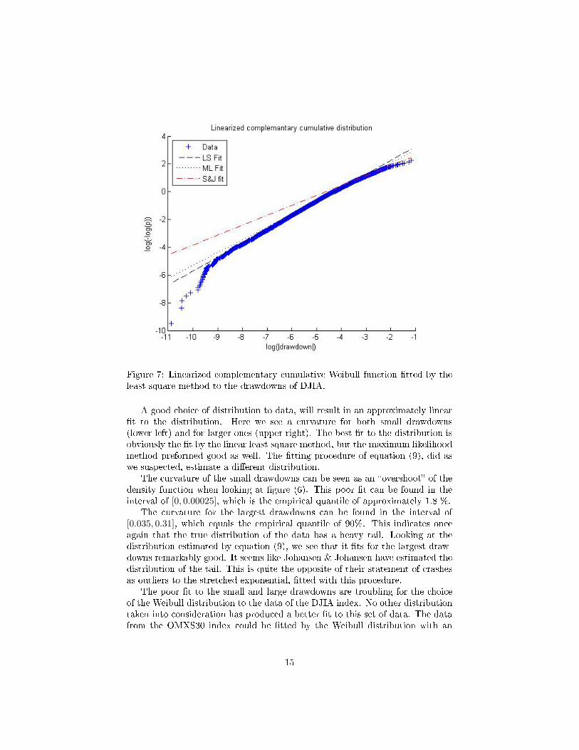
Figure 7: Linearized complementary cumulative Weibull function �tted by theleast square method to the drawdowns of DJIA.

A good choice of distribution to data, will result in an approximately linear�t to the distribution. Here we see a curvature for both small drawdowns(lower left) and for larger ones (upper right). The best �t to the distribution isobviously the �t by the linear least square method, but the maximum likelihoodmethod preformed good as well. The �tting procedure of equation (9), did aswe suspected, estimate a di�erent distribution.

The curvature of the small drawdowns can be seen as an �overshoot� of thedensity function when looking at �gure (6). This poor �t can be found in theinterval of [0, 0.00025], which is the empirical quantile of approximately 1.8 %.

The curvature for the largest drawdowns can be found in the interval of[0.035, 0.31], which equals the empirical quantile of 90%. This indicates onceagain that the true distribution of the data has a heavy tail. Looking at thedistribution estimated by equation (9), we see that it �ts for the largest draw-downs remarkably good. It seems like Johansen & Johansen have estimated thedistribution of the tail. This is quite the opposite of their statement of crashesas outliers to the stretched exponential, �tted with this procedure.

The poor �t to the small and large drawdowns are troubling for the choiceof the Weibull distribution to the data of the DJIA index. No other distributiontaken into consideration has produced a better �t to this set of data. The datafrom the OMXS30 index could be �tted by the Weibull distribution with an

15

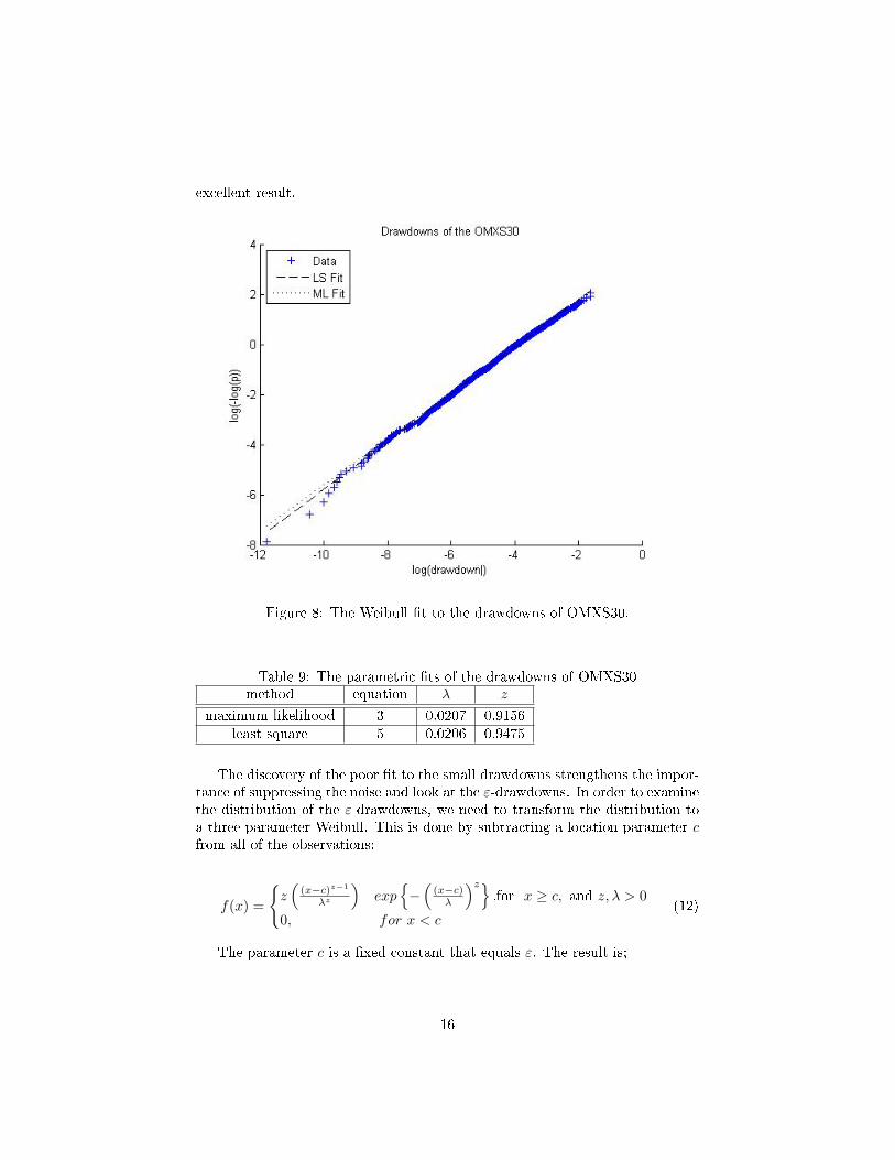
excellent result.

Figure 8: The Weibull �t to the drawdowns of OMXS30.

Table 9: The parametric �ts of the drawdowns of OMXS30method equation λ z

maximum likelihood 3 0.0207 0.9156least square 5 0.0206 0.9475

The discovery of the poor �t to the small drawdowns strengthens the impor-tance of suppressing the noise and look at the ε-drawdowns. In order to examinethe distribution of the ε-drawdowns, we need to transform the distribution toa three parameter Weibull. This is done by subtracting a location parameter cfrom all of the observations;

f(x) =

{z(

(x−c)z−1

λz

)exp

{−(

(x−c)λ

)z},for x ≥ c, and z, λ > 0

0, for x < c(12)

The parameter c is a �xed constant that equals ε. The result is;

16

Table 10: The estimates of the three parameter Weibull. Here c = 3σ = 0.0345.method equation λ z

least square 5 0.0466 0.9816maximum likelihood 3 0.0460 1.0280

Figure 9: The complementary cumulative distribution of the ε-drawdowns ofthe DJIA index.

The �t to the epsilon-drawdowns is excellent, hence we have a good modelfor the distribution of trends.

We will make a new de�nition of crashes, with the bene�t of not being de-pendent on any speci�c distribution. We de�ne a crash as the 99.50% empiricalquantile of the drawdowns. For the drawdowns of the DJIA is 10.50%, andfor OMXS30 is 12.48%. Severe crashes are rare and do not occur very often.When a crash occurs, it is often associated with a drawdown larger than 10 %.Looking at the 99.5% quantile, all of the drawdowns are larger than 10% andthe corresponding dates are historical events of �nancial crashes.

17

3 The model

The regime of a growth era can end in three ways; the regime can switchsmoothly, it can end with a crash, or turning into an anti-bubble. Hence, acrash is not a deterministic outcome and has a probability of happen, or theregime can switch smoothly. The theory of this chapter is the model proposedby Sornette [10] and Johansen and et. al. [7], as the underlying mechanismof the log-periodic oscillation. We will start with some human characteristicsthat play a key role in choice of best strategy, when optimizing the pro�t. Bymodeling the best strategy in a macroscopic way and combining this with pricedynamics, we can derive the equation of the LPPL signatures.

3.1 Feedback

Any price on a stock market �uctuates by the law of supply and demand. Wecan also describe the �uctuations of the price as a �ght between order anddisorder.

An agent on a stock market has three choices to consider; sell, buy or wait.During normal times on a stock market disorder rules, implying there are asmany sellers as buyers and that the agents do not agree with one another. Acrash happens when order rules, and too many agents want to sell at the sametime. In times of a crash, the market gets organized and synchronized, which isquite the opposite of the common characterization of crashes as times at chaos.The question is, what mechanism can lead to an organized and coordinated sello�?

All traders in the world are organized into networks of family, friends, col-leagues, etc. that in�uence each other by their opinions of whether to buy orsell. The optimal strategy for an agent on a stock market, with lack of infor-mation of how to act, is to imitate what others do, since the opinion of themajority will move the prices in that direction.

Trends on a stock market arise from feedback, that for a speculative bubbleis positive and for an anti-bubble are negative. Feedback describes the situationwhere the output from a past event will in�uence the same situation in thepresent. Positive feedback, which moves the system in the same direction asthe positive signal, is known as self-reinforcing loops and that drives a systemout of equilibrium. In a stock market, positive feedback leads to speculativetrends, which may dominate over fundamental and rational beliefs. A specula-tive bubble is a system driven out of equilibrium, and it is very vulnerable toany exogenous shock, that could trigger a crash. In real world, positive feedbackis controlled by negative feedback as a limiting factor, and positive feedback donot necessarily result in a runway process.

3.1.1 Herding and imitation

Feedback are the cause of two psychological factors; herding and imitation.

18

Herding behavior occurs in everyday decision making, based on learningfrom others. The phenomenon is called information cascade and is also knownas the Bandwagon e�ect in economics. This occurs when people observe theactions made by others and then make the same choice, independently of theirown private beliefs. The main cause of this behavior is lack of information andthe belief that they are better o� mimicking others. Some people choose toignore and downplay their own personal beliefs, rather than acting on them,because of the strong opinion of the crowd. As more people come to believein something, others choose to �jump on the bandwagon�, regardless of theevidence supporting the action, and the information cascade will spread with adomino-like e�ect.

People are rational and will always aim to maximize their utility. Whenpeople know that they are acting on limited information, they are willing tochange that behavior. A single new piece of information can make a lot ofpeople to subsequently choose a di�erent action and in an instant turnover aprevious established trend of acting. Therefore, information cascades are veryfragile.

3.2 Microscopic modeling

Consider a network of agents and denote each one of them with an integeri = 1, ..., I. Let N(i) be the set of agents that are directly connected with agenti. According to the concepts of herding and imitation, the agents in N(i) willin�uence each other. Say we isolate one single trader i, and the network N(i)consisting of j = 1, . . . , n individuals surrounding that trader.

For every unit of time, each member in the network will be in one of twopossible states; selling = −1 or buying = +1, which could represent beingpessimistic or positive.

The sum of all agents on the market∑Ni=1 si will move the price proportion-

ally, where s denotes the two states selling of bying. The best choice when thesum is negative is to sell and buy when the sum is positive. If the sum is zero,there are as many buyers as sellers, and the price should not change. Since thissum is unknown to the single trader, the best strategy that will maximize thereturn, is polling the known neighborhood and hopefully this sample will be arepresentation of the whole market. The trader has to form a priori distributionof the probability for each trader selling P− and buying P+. The simplest casecorrespond to a market with no drift, P− = P+

The general opinion in a network of a single trader is given by∑nj=1 sj .

The optimal choice is given by:

si(t+ 1) = sign

K n∑j=1

sj(t) + σεi

(13)

where ε is a N(0, 1)-distributed error compensating that the network did notrepresent the whole market correctly. K is a positive constant measuring thestrength of imitation. The variable K is inversely proportional to the market

19

depth, which gives the relative impact of a given unbalance of the aggregatedbuy and sells orders, depending on the size of the market; the larger market, thesmaller impact of a given unbalance. σ governs the tendency toward idiosyn-cratic behavior, and together with the constant K, it determines the outcomeof the battle between order and disorder on the market.

3.3 Macroscopic modeling

The variable K measures the strength of imitation and there exists a variableKc that determines the property of the system of imitation. When K < Kc,disorder rules on the market, and the agents are are not agreeing with oneanother. As K gets closer to Kc, order starts appearing where agents whoagree with each other form large groups, and the behavior of imitation is widelyspread. At this point, the system is extremely unstable and sensitive to anysmall global permutation that may result in large collective behavior triggeringa rally or a crash. It should be stressed that Kc is not the value for the crashto happen, it could happen anyway at any level of K, but the probability of thecrash is not very likely for small values of K. In Natural Science, this is knownas a critical phenomenon. The hallmark of a critical phenomenon is a powerlaw, where the susceptibility goes to in�nity. The susceptibility is given by:

χ ≈ A (Kc −K)−γ (14)

where A is a positive constant and γ is called the critical exponent.Sornette & Johansen [7] model this imitation process by de�ning a crash

hazard rate evolving over time. The critical point is now tc, which is the mostprobable time of the crash to take place, and the death of a speculative bubble.

h(t) = B (tc − t)−α (15)

where t denotes the time and B is a positive constant. The exponent is givenby α = (ξ− 1)−1, where ξ is the number of traders in one typical network. Thetypical trader must be connected to at least one other trader, hence 2 < ξ <∞.This result is an exponent that will always be smaller than one and the pricewill not continue to in�nity.

There exists a probability:

1−tcˆ

t0

h(t)dt > 0 (16)

that the crash will not take place and the speculative bubble will land smoothly.Hence, we see that the hazard rate behaves in the similar way as the approxi-mated susceptibility.

20

3.4 Price dynamics

For simplicity of the model, Johansen & Sornette [7] choose to ignore interestrate, dividends, risk aversion, information asymmetry, and the market clearingcondition.

The rational expectation model says that in an e�cient market every agenttakes all pieces of available information, looking rational into the future tryingto maximize their well being. The aggregated predictions of the future pricewill be the expected value conditioned of the information revealed up to time t,which will be the price of the asset at time t. This gives the famous martingalehypothesis of rational expectations:

Et[p(t′)] = p(t), for all t′ > t (17)

In a maket without noise, we get the solution of the martingale equation p(t) =p(t0) = 0, where t0 denotes the initial time. The rational expectation modelcan be interpreted as price in excess of the fundamental value and for a positivevalue of p(t) that constitutes a speculative bubble.

Assume for simplicity that when the crash takes place, the price drops by a�xed percentage κ ∈ (0, 1) . The dynamics of the price of an asset before thecrash is given by:

dp = µ(t)p(t)dt− κp(t)dj (18)

where j denotes a jump process taking the value 0 before the crash and 1afterwards. The drift coe�cient µ(t) is chosen so that the martingale conditionis satis�ed:

Et[dp] = µ(t)p(t)dt− κp(t)h(t)dt = 0 (19)

This yields:

µ(t) = κh(t) (20)

The martingale condition states that investors must be compensated by a highreturn of the assets price to keep invested, when the probability of a crash rises.Hence, when the price rises, the risk of a crash increases, therefore is no suchthing as a free lunch. Plugging equation (20) into equation (18) gives:

dp = κh(t)p(t)dt− κh(t)dj (21)

When j=0 before the crash, we get an ordinary di�erential equation

p′(t) = κh(t)p(t)

p′(t)p(t)

= κh(t) (22)

Integrating equation (22) on both sides gives the corresponding solution beforethe crash:

21

log[p(t)p(t0)

]= κ

tˆ

t0

h(t′)dt′

log(p(t)) = log(p(t0)) + κ

tˆ

t0

h(t′)dt′ (23)

where

tˆ

t0

h(t′)dt′ = B

tˆ

t0

(tc − t′)−α

dt = −B[

(tc − t′)−(α+1)

α+ 1

]t′=tt′=t

=

= −B(

2tc − t− t0α+ 1

)= {let t0 = tc and β = α+ 1 ∈ (0, 1)} = −B

β(tc − t)β

(24)Plug equation (24) into equation (23):

log(p(t)) = log(p(to))−κB

β(tc − t)β (25)

We have now reached the �nal step of deriving the equation of the Log-Periodicformula. Recall equation (14) of the susceptibility of the system χ ≈ A (Kc −K)−γ

that we imitated by the hazard rate. We will make the assumption of the sus-ceptibility of the system to be a bit more realistic, by letting the exponent of thepower law be a complex number. When the exponent is a complex number, onecan model a system with hierarchical structures in a network. In the real world,this is a more accurate way of describing the market, since di�erent agents holddi�erent amounts of shares and their decision of buying and selling has di�erentimpact on the market. The most powerful agents on the market, who are onthe top of the hierarchy holding large amounts of shares, are pension funds etc.A more general version of the equation describing the susceptibility is sums ofterms like, χ ≈ A (Kc −K)−γwith complex exponents.

χ ≈ Re[A0 (Kc −K)−γ +A1 (Kc −K)−γ+iω + ...

]≈

≈ A′0 (Kc −K)−γ +A′1 (Kc −K)−γ cos(ω log(Kc −K) + ψ)... (26)

where A′0, A′1, ω and ψ are real numbers, and Re[] denotes the real part of

a complex number. These accelerating oscillations are called log-periodic, andtheir frequency are λ = ω/2π.

Following the same step, we can back up the hazard rate:

h(t) ≈ Re[B0 (tc − t)−γ +B1 (tc − t)−γ+iω + ...

]≈

≈ B′0 (tc − t)−γ +B′1 (tc − t)−γ cos(ω log(tc − t) + ψ) (27)

22

Plugging equation (27) into equation (25), we get the evolution of the pricebefore the crash:

log(p(t)) = log(p(to))−κ

β

(B0 (tc − t)β +B′1 (tc − t)−γ cos(ω log(tc − t) + ψ)

)(28)

Simplifying this gives:

y = A+B (tc − t)z + C (tc − t)z cos (ω log (tc − t) + Φ)

and we now have the same expression as equation (1).

3.5 The equation

Following the recommendations of Gazola, Fernandez, Pizzinga, Riera [3], thequali�cation of the parameters in the equation (1) will be:

y(t) should be the logarithm of the price if we follow the derived formula.Indeed, the LPPL-equation may be �tted to any choice of presentation of the�nancial data such as price at closure or normated prices.

A has to be larger than zero and equals the predicted price of the asset atthe time of the crash p(tc). For a bullish speculative bubble and for a bearishanti-bubble B has to be smaller than zero. If B is larger than zero in case of ananti-bubble, this is referred to as a bullish anti-bubble and is discussed in Zhou& Sornette [13]. C 6= 0 to ensure the log-periodic behavior.

The parameter tc is the most probable time of the crash, if it actually occurs.z will lie between [0, 1] and the empirical �ndings of J&S [6] for speculative

bubbles are z = 0.33± 0.18.ω controls the amplitude in the oscillations and will lie between [5, 15]. The

empirical �ndings of J&S [6] for speculative bubbles are ω = 6.36± 1.56.φ has not been considered elsewere, but for Gazola el. al. [3] it is assumed

to be [0, 2π].A, B, C and Φ are simply units and carry no structural information.Equation (1) exempli�es two characteristics of a bubble with a preceding

endogenous crash:

∗ A growth that is faster than an exponential growth, which is captured bythe power law B (tc − t)z.

∗ An accelerating oscillation decorating the power law quanti�ed by theterm cos (ω log (tc − t) + Φ).

23

4 The �tting process

Fitting a set of �nancial data to a complex equation, like equation (1), involvesa number of considerations to secure that the best possible �t is being obtained.

4.1 Number of free parameters

In order to reduce the number of free parameters in the �t, the three linearvariables have been �slaved� into the �tting procedure and calculated from theobtained values of the nonlinear parameters, suggested by Sornette & Johansen[7]. This is done by rewriting equation (1) as:

y(t) ≈ A+Bf(t) + Cg(t) (29)

where

f(t) =

{(tc − t)z for a speculative bubble

(t− tc)z for an anti-bubble(30)

g(t) =

{cos (ω log (tc − t) + Φ) for a speculative bubble

cos (ω log (t− tc) + Φ) for an anti-bubble(31)

For each choice of the nonlinear parameters, we obtain the best values of thelinear parameters by using ordinary least square (OLS) method:

∑Ni y(ti)∑N

i y(ti)f(ti)∑Ni y(ti)g(ti)

=

N∑Ni f(ti)

∑Ni g(ti)∑N

i f(ti)∑Ni f(ti)2

∑Ni f(ti)g(ti)∑N

i g(ti)∑Ni f(ti)g(ti)

∑Ni g(ti)2

A

BC

(32)

We write this system of equations in a compact representation:

X′y = (X′X)b (33)

where X =

1 f(t1) g(t1)...

......

1 f(tn) g(tn)

and b =

ABC

The general solution of this eqaution is:

b = (X′X)−1X′y (34)

This leaves four physical parameters controlling the �t.

24

4.2 The optimization problem

Fitting a function to data is a minimization of the residual sum of squares, SSE,which is the objective function given by:

minθF (θ) =

N∑i

(yθ(ti)− yθ(ti))2 ,where θ = (tc, φ, ω, z) (35)

The function of the residual sum of squares, F (θ) is not a well behaved convexfunction and consists of multiple local minimums with fairly similar values. Theconsideration is to �nd the global minimum, which is the local minimum withthe smallest value.

The unconstrained global optimization problem, A. Georgiva & I. Jordanov[4], is de�ned as to �nd a point P ∗ ∈ Π from a non empty, compact feasibleinterval domain Π ⊂ Rn that minimizes the objective function F :

F ∗ = F (P ∗) ≤ F (P ), for all P ∈ Π (36)

where F ∗ : Rn → RWorking in a parameter space of four nonlinear parameters, one cannot get atrue picture of the characteristics of the objective function. To demonstratethe problems with optimizing the objective function, we use data from thespeculative bubble of the DJIA that ended with a crash in October 1929. Welet two parameters vary and keep the rest of the nonlinear parameters �xed.The parameters are varying over the given intervals, but now we let φ vary over[−2π, 2π]. The linear parameters are estimated by equation (34).

Figure 10: The objective function when Φ and ω are varying.

25

Figure 11: The objective function when ω and tc are varying.

Figure 12: The objective function when Φ and z are varying.

With these plots it becomes clear when trying to optimize the objectivefunction with methods like the downhill simplex method or the Quasi-Newtonmethod, we risk to get trapped in local minimum, rather than �nding the globalminimum. These methods are a very e�cient, but they can only �nd the localminimum in the basin of attraction in which the initial starting point is set at.How can we set the initial starting points in the right basin of attraction when

26

we do not know where the global minimum is at? There are many ways to solvea global optimization problem such as Simulated Annealing, Taboo Search andGenetic Algorithm etc. The Genetic Algorithm was used here.

4.3 Genetic Algorithm

The Genetic Algorithm, GA, is an evolutionary algorithm inspired by Darwin's�survival of the �ttest idea�. The theory of the GA was developed by JohnHolland, known as the father of GA by his pioneer work in 1975.

The GA is a computer simulation that mimics the natural selection in bio-logical systems governed by a selection mechanism, a crossover (breeding) mech-anism, a mutation mechanism, and a culling mechanism. There are many waysto apply the mechanisms of the GA, here we follow the guidelines of Gulsten,Smith & Tate [5].

Algorithm 1 A pseudo code for the Genetic Algorithm

1. Randomly generate an initial solution set (population) and calculate thevalue of the objective function.

2. Repeat {

Select Parents for crossover.

Generate o�spring.

Mutate some of the members of the original population.

Merge mutants and o�spring to into the population.

Cull some members of the population to maintain constant populationsize.

}

3. Continue until desired termination criterion is met.

The main bene�ts of the GA are that no special information about thesolution surface is needed, such as gradient or curvature. The objective functiondo not need to be smooth or continuous. The GA has been proven to be robustin �nding the parameter values in the objective function.

4.3.1 Generating the initial population

Each member of the population is a vector of our coe�cients (tc, φ, ω, z). Theinitial population consists of members with coe�cients drawn at random, from auniform distribution with a pre-speci�ed range. The population has 50 membersand the �tness value, the residual sum of squares, is calculated for each member.

27

4.3.2 Breeding mechanism

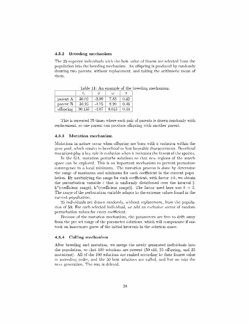
The 25 superior individuals with the best value of �tness are selected from thepopulation into the breeding mechanism. An o�spring is produced by randomlydrawing two parents, without replacement, and taking the arithmetic mean ofthem.

Table 11: An example of the breeding mechanism.tc φ ω z

parent A 30.02 -3.99 7.83 0.42parent B 30.25 -4.15 8.20 0.46o�spring 30.135 -4.07 8.015 0.44

This is repeated 25 times where each pair of parents is drawn randomly withreplacement, so one parent can produce o�spring with another parent.

4.3.3 Mutation mechanism

Mutations in nature occur when o�spring are born with a variation within thegene pool, which results in bene�cial or less favorable characteristics. Bene�cialmutations play a key role in evolution when it increases the �tness of the species.

In the GA, mutation perturbs solutions so that new regions of the searchspace can be explored. This is an important mechanism to prevent prematureconvergence in a local minimum. The mutation process is done by determinethe range of maximum and minimum for each coe�cient in the current popu-lation. By multiplying the range for each coe�cient, with factor ±k, we obtainthe perturbation variable ε that is uniformly distributed over the interval [-k*(coe�cient range), k*(coe�cient range)]. The factor used here was k = 2.The range of the perbutation variable adapts to the extreme values found in thecurrent popultation.

25 individuals are drawn randomly, without replacement, from the popula-tion of 50. For each selected individual, we add an exclusive vector of randomperturbation values for every coe�cient.

Because of the mutation mechanism, the parameters are free to drift awayfrom the pre-set range of the parameter solutions, which will compensate if onetook an inaccurate guess of the initial intervals in the solution space.

4.3.4 Culling mechanism

After breeding and mutation, we merge the newly generated individuals intothe population, so that 100 solutions are present (50 old, 25 o�spring, and 25mutations). All of the 100 solutions are ranked according to their �tness valuein ascending order, and the 50 best solutions are culled, and live on into thenext generation. The rest is deleted.

28

4.3.5 A demonstration of the Genetic Algorithm

Recall �gure (11), when we let tc and ω vary. We will perform an optimization

of the objective function minθF (θ) =

∑Ni (yθ(ti)− yθ(ti))2 ,where θ = (tc, ω),

using the Genetic Algorithm. The rest of the parameters are �xed. Here wehave used the population size to 40 and the elite- and mutation number is 10.The algorithm is iterated 10 times after the initial population is created. Thefollowing pictures shows how the algorithm �nds the global minimum.

29

Figure 13: A demonstration of the Genetic Algorithm, when optimizing for tcand ω. The algorithm is iterated 10 times and the generations in the picturesare from the upper left and down; the initial randomly drawn population andthen generation number 2,4,6,8 and 10.

30

4.3.6 Hybrid Genetic Algorithm

To improve and guarantee the best result of the parameter estimation we apply aNelder-Mead Simplex method, also known as the downhill simplex method, withthe estimated parameters from the GA as the initial values. We use the sameobjective function as for the Genetic Algorithm, when estimating the nonlinearparamaters with the downhill simplex method.

.

Figure 14: A demonstration how the GA improves the best value of �tness forthe objective function over generations. Generation number 51 is the Nelder-Mead Simplex method improving the result with the estimated parameters fromthe GA as initial values. The LPPL-equation is �tted to the speculative bubbleseen in DJIA that ended in a crash 1929.

4.4 Fitting the LPPL equation

Fitting the LPPL equation to historical data of a speculative bubble, one typ-ically chooses the window of estimation with the start at the point where theLPPL signatures �rst seem to appear, and the peak of the price as the end.Including the data of the crash will be less favorable to the �t, and one risk isto hit the point of tc, with the result of complex numbers that will destroy the�t. When �tting the LPPL equation for the purpose of prediction, the start willbe at the point where the signatures start and then use all available data.

Fitting the LPPL equation to an anti-bubble, the �tting procedure is pre-ceded in a di�erent manner. For a speculative bubble, the end of the curve is at

31

the point of tc, recall (tc − t). The parameter tc for an anti-bubble is the startof the LPPL signatures, hence (tc − t).

The consideration is where to set the start of the window of estimation foran anti-bubble. If we knew the time tc, then the obvious choice would be a tstartnext to tc, which is the most optimal choice when it allows us to use the longestpossible time span. Not knowing the critical time precisely, we have to ensurethat tc < tstart to avoid complex numbers and ensure an accurate �t. This canresult in a bit of work testing for di�erent times of tstart, by trial and error.

If we remove the constraint tc < tstart, by taking the absolute value of |tc−t|,it is possible to scan for di�erent tstart and attain a �exibility in the search spaceof tc.

When optimizing with this new procedure, we use the peak as the start ofthe window of estimation, or at the point where the LPPL signature �rst seemto appear. The end is at the bottom of the anti-bubble for historical data, orthe data available when �tting a current anti-bubble.

The �ts produced by this new procedure are robust and stable, but facesome minor problems. Adding an absolute value operator into the equation, itis assumed that an anti-bubble is always associated with a symmetric bubblewith the same parameters, and the same value of tc. This is not true, but wechoose to neglect this when tc with this new procedure often is very close totstart, according to Sornette & Zhou [12]. A value tc much larger than tstartwill compromise the �t, as the GA is trying to optimize the symmetric bubble.If this happens, choose a larger value of tstart.

Another consideration about the optimization of the objective function,equation (35) is the presence of multiple local minimum with approximatelythe same value of �tness.

Table 12: Multiple local minimums with approximately the same �tness value. Here we optimize the parameters of the LPPL equation to the speculativebubble of DJIA, prior to the crash in October 1929. We optimize the equationover the standard intervals, but let φ take values in the interval [−2π, 2π].

R2 A B C tc φ ω z

0.98307160189274 590.2883 -285.8670 -14.2892 30.2247 2.0879 7.9276 0.42040.98307160189287 590.2909 -285.8691 14.2892 30.2247 -1.0537 7.9276 0.42030.98307160189315 590.2842 -285.8628 14.2892 30.2247 5.2295 7.9276 0.42040.98307160189311 590.2804 -285.8596 -14.2892 30.2247 -4.1952 7.9276 0.4204

5 Results

This chapter presents the results of �tting the LPPL-equation to di�erent �-nancial time series. We follow the guidelines of Johansen & Sornette [6] whensearching for the LPPL signature in �nancial time series. We look at the largestdrawdowns and look at the time series preceding them. The ambition is to �ndthe LPPL signature in the time series before and within the current �nancial

32

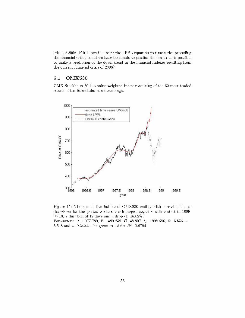
crisis of 2008. If it is possible to �t the LPPL-equation to time series precedingthe �nancial crisis, could we have been able to predict the crash? Is it possibleto make a prediction of the down trend in the �nancial indexes resulting fromthe current �nancial crisis of 2008?

5.1 OMXS30

OMX Stockholm 30 is a value weighted index consisting of the 30 most tradedstocks of the Stockholm stock exchange.

Figure 15: The speculative bubble of OMXS30 ending with a crash. The ε-drawdown for this period is the seventh largest negative with a start in 1998-08-18, a duration of 12 days and a drop of -16.02%.Parameters: A=1077.799, B=-489.258, C=48.907, tc=1998.686, Φ=5.556, ω=5.518 and z=0.3424. The goodness of �t: R2=0.9794

33

Figure 16: The LPPL-equation �tted to OMXS30. The crash of the new econ-omy resulted in an anti-bubble that spread world wide a�ecting the OMXS30.The bottom of the anti-bubble was predicted by a local minimum of the LPPLequation.Parameters: A=1299.98, B=-493.427, C=78.805, tc=2000.74885, Φ=3.478,ω=8.982 and 0.4934.The goodness of �t: R2=0.961

34

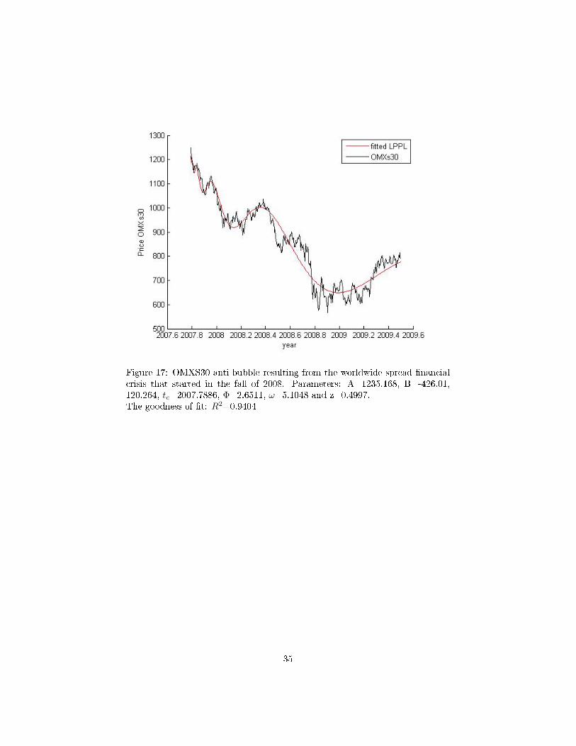
Figure 17: OMXS30 anti-bubble resulting from the worldwide spread �nancialcrisis that started in the fall of 2008. Parameters: A=1235.168, B=-426.01,120.264, tc=2007.7886, Φ=2.6511, ω=5.1048 and z=0.4997.The goodness of �t: R2=0.9404

35

Figure 18: The LPPL �tted to OMXS30 for the anti-bubble resulting from the�nancial crisis of 2008. The curve is plotted over a longer time span with thenext local minimum in the end of 2011.

36

The LPPL equation could absolutely not be �tted to the time span prior to thecrash of the New Economy, nor the �nancial crisis of 2008. The growth of theperiods resembles linear trends.

Figure 19: The price development of OMXS30.

5.2 DJIA

The Dow Jones Industrial average was founded in 1896 and represented theprice average of the 12 most important industrial stocks in the United States.Today the DJIA has little to do with the traditional heavy industry and is aweighted price average of the 30 largest and most widely held public companies.

37

Figure 20: The speculative bubble of DJIA that ended with a crash in 1987-10-13. DJIA fell during the Black Monday of October 19, 1987 with -22.61 %. Thedrawdown for this crash is -30.68% and is the largest drawdown the DJIA hasexperienced.Parameters: A=4047.71, B=-1997.52, C=101.831, tc=1988.00, Φ=2.018, ω=8.471 and z=0.327.The goodness of �t: R2=0.9872

38

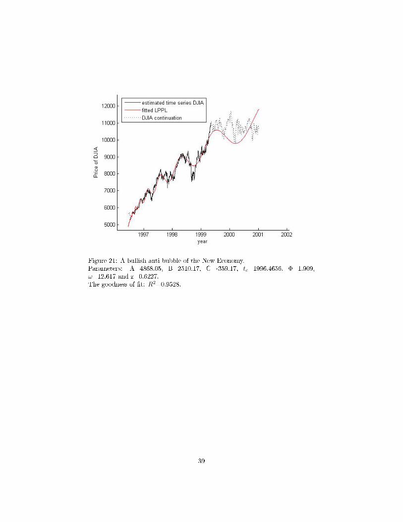
Figure 21: A bullish anti-bubble of the New Economy.Parameters: A=4868.05, B=2510.17, C=-359.17, tc=1996.4656, Φ=1.909,ω=12.617 and z=0.6227.The goodness of �t: R2=0.9528.

39

Figure 22: The anti-bubble of DJIA after the crash of the New Economy in2000.Parameters: A=10957.03, B=-863.55, C=-522.31, tc=2000.63, Φ=5.0673, ω=9.611 and z=1.043.The goodness of �t: R2=0.8415

Figure 23: The LPPL signatures found before the �nancial crisis in 2008.Parameters: A=19148.19, B=-7024.61, C=-283.499, tc=2007.967, Φ=3.245, ω=10.205 and z=0.2910.The goodness of �t: R2=0.9737

40

The bubble of the New Economy, also known as the �dot-com� bubble, isone of the most famous speculative bubbles in the world. Failing to �t theLPPL-equation for a speculative bubble for some time series prior to the crash,the equation for an anti-bubble could be �tted. This is known as a bullishanti-bubble with the parameter tc indicating the start of the anti-bubble. Thebullish anti-bubble has a positive slope. Like the bearish anti-bubble, there is nopossibility to make a prediction at the end of the anti-bubble. The appearanceof the bullish anti-bubble in one of the most famous bubbles is an interestingfeature.

DJIA did a fast recovery after the bottom of the anti-bubble of 2000. Be-tween January 2004 and October 2005, the DJIA hits a plateau with slow devel-opment and the LPPL signatures were found in the time span of 2005-10-06 to2007-07-13. An endogenous bubble is consistent with an immediate crash withlarge drawdowns. Indeed, the time period of 2008-2009 did contain some of thelargest drawdowns of DJIA, but they were delayed. The �t of the peak is notthat perfect either. One can argue whether this is a true endogenous bubble oran exogenous shock. The time span of 2008-2009 can absolutely not be �ttedto the LPPL equation as an anti-bubble.

5.3 S&P500

Standard & Poor 500 is a value weighted index published in 1957 of the prices ofthe largest 500 American large-cap stocks. It is one of the most widely followedindexes in the world and is considered to re�ect the wealth of the US economy.The data used for the curve �ts are S&P500 Total Return, which re�ects thee�ects of dividends reinvested in the market.

41

Figure 24: The speculative bubble in S&P500 ending in a crash with a drawdownof -13.21 % in 1998-08-24.Parameters: A=3636.24, B=-950.388, C=146.00, tc=1998.7903, Φ=5.010,ω=7.4305 and z=0.9561 .The goodness of �t: R2=0.9768

Figure 25: The anti-bubble resulting from the crash of the new economy in 2000.Parameters: A=4630.459, B=-1092.43, C=-213.488, tc=2000.6318, Φ=5.21089,ω=9.918 and z=0.540.The goodness of �t: R2=0.9429

42

Figure 26: The LPPL �t to the time series of S&P500 prior the �nancial crisisof 2008.Parameters: A=5543.743, B=-1124.797, C=137.258, tc=2007.6976, Φ=2.236,ω=6.935 and z=0.6458. The goodness of �t: R2=0.9793

As for DJIA this �t can be questioned if it is really a speculative bubble oran exogenous shock. The LPPL-equation could not be �tted to the time seriesof the �nancial crisis of 2008.

6 Discussion

Looking at drawdowns rather than daily returns is a good alternative to examinethe �uctuations of the price in a �nancial market. The beauty of �tting adistribution to data is the possibility to calculate probabilities of future events,based on the distribution of historical data. To be able to �t a distribution tothese movements results in a good tool for i.e. risk management. Instead oftrying to prove that crashes are outliers as Johansen & Sornette [6], we wouldbe better o� trying to �t these observations to a distribution.

Johansen & Sornette [6] used an unusual �tting procedure to estimate the pa-rameters of the stretched exponential. By a linearization of the complementarycumulative Weibull distribution, we concluded that the parameter estimatesfrom this �tting procedure did not result in a good �t to the data. In fact, thelogarithmic transformation used in equation (9) is not a good transformation to�t the parameters of the distribution. A good transformation of a function willresult in robust estimates of the parameters, and this transformation fails.

We could �t the Weibull distribution with a very good result to the draw-

43

downs of the OMXS30 index. The drawdowns of DJIA could not be �tted aswell as for the OMXS30 index. The Weibull distribution could not extrapolatethe small and large drawdowns, resulting in a curvature. The bad �t to theWeibull distribution could indicate some sort of mixture model, or a heavy tailof the true distribution. We stress that this does not prove the point of Johansen& Sornette [6] that crashes are outliers. The curvature starts at the drawdownsize of 3.5% and that is not considered as a crash in a stock market.

The curvature may also be a result of noise. By suppressing noise in �nancialtime series, it is possible to obtain more continuous drawdowns with two mainbene�ts; we prove that the largest drawdowns are in fact the largest ones, andwe can obtain a better �t to a distribution.

Very few guidelines about the ε-drawdown algorithm used by Johansen &Sornette [6] were given and their results could not be replicated. Looking at theirplots in of the ε-drawdowns it becomes clear that they do not treat drawups asdrawdowns, when they include drawdowns smaller than ε. With their treatmentof the ε-drawdowns, they faced some problems; �Those very few drawdowns(drawups) initiated with this algorithm which end up as drawups are discarded�,Johansen & Sornette [6]. Not a single observation had to be discarded with ouralgorithm because of positive signs for the ε-drawdowns and our interpretationof the problem must be slightly better. Not treating the ε-drawups like ε-drawdowns may result in an incorrect distribution of trends.

A concern is how to choose a good value of ε. Johansen & Sornette [6] suggestthat the volatility is the factor that should be used to suppress the noise in�nancial time series. The volatility is calculated as the standard deviation of thelogarithmic returns between successive days, and the drawdowns are calculatedas the percentage drop from a local maximum to the following local minimum.Even though we have replicated their work, we believe that comparing onemeasurement with another is fundamentally wrong. A better value of epsilonwould probably be the volatility of the daily returns calculated in precentage,eventhough the di�erence between these two measurements is quite small. Byletting the value of ε be large enough, it is possible to �t the ε-drawdowns to athree-parameter Weibull distribution with an excellent result.

A common de�nition of a speculative bubble is when the price of an index orasset rise signi�cantly over a short period of time and becomes overvalued, end-ing with a crash. Above this de�nition, there are many models and de�nitionsof a speculative bubble. Some even argue if there is such thing as a speculativebubble. Johansen & Sornette have developed their de�nition of an endogenousspeculative bubble exhibiting the LPPL oscillation. We cannot argue that theseLPPL-signatures do not exist, but the main question is why they exist. Is it infact a result of a feedback loop driven by imitation and herding, leading to acollapse in one critical instant? Can the explanation simply be that the LPPLsignature is a result of an accidental feature of the stochastic process that drivesthe price on a �nancial market?

The most famous speculative bubble was the �dot-com� bubble in 1998-2000. If we study the development of the ending years of the �dot-com� bubblein OMXS30, DJIA and S&P500, there are approximately linear trends and no

44

signs of the LPPL-signatures.The LPPL equation could be �tted to the DJIA and S&P500 prior to the

current �nancial crisis of 2008, but are the �ts just accidental? We know that the�nancial crisis of 2008 originated from a speculative bubble in the credit market.This speculative bubble in�ated when the credit market were suppressing risksand aiming for larger pro�ts. In the United States the credit market bubblewas a result of a house market bubble, which peaked approximately in 2005-2006. We know that the price development in a stock market is the resultthe information interpreted by analyst and traders. Therefore the speculativebubble of the housing and credit market ought to a�ect the American stockmarket as well.

The de�nition made by Johansen & Sornette [6], is that a speculative bubble,exhibiting the LPPL signature, should have its crash at some time t ≤ tc. If thecrash does not occur, the ending of the speculative bubble is to be consideredas a soft landing. An exogenous crash can be preceded by any development ofthe price. Can the �nancial crisis be considered as a burst of an endogenousbubble?

The concern is about the development of the indices of the S&P500 and theDJIA prior to the �nancial crisis of 2008. The LPPL equation could be �ttedto both of the indices, but not to the highest peak. Using the second highestpeak in the window of estimation, the model predicted the turning point atthe highest peak. At �rst, the indices began to decline slowly, which indicatesa slow landing of the speculative bubble. Looking at the time series after theturning point, the severe crashes of the indices looks like the de�nition of anexogenous crash. We do not consider the �nancial crisis as an exogenous event,and we believe the model simply failed to predict the crash, that was delayed.Nevertheless, the model accurately predicted the turning point at the maximumpeak.

How well does this model perform when predicting crashes? There are twomajor problems of the model:

∗ When looking at the plots . of the estimated LPPL curve, it becomes clearthat the parameter tc overshoots the actual time of the crash. Sornetteet. al. [7], defend this by the rational expectation model and stress thatthe probability of a crash increases as the time approaches tc and that tcis the most probable time of a crash.

∗ Another concern is how much time prior to the peak of a speculativebubble that is needed to obtain an accurate estimation of the parametertc .

According to Sornette et. al. [7], it is possible to lock in the parameter tc up toa year prior to the time of crash. They used data from a speculative bubble inS&P500 over the time period of January 1980 to Sepeptember 1987 that couldbe �tted by a LPPL curve containing 6 local maximum. They took the enddate of 1985.5 and added 0.16 years consecutively to the time of the crash. Thenumber of oscillations varied between the di�erent �ts, meaning the appearance

45

of the curve varied, but the parameter tc were quite robust. It is possible tomake this statement by choosing a long speculative bubble with many oscilla-tions. Detecting a LPPL signature in �nancial data requires at least two localmaximum or two local minimum. Many of the speculative bubbles only containbetween 2-4 local maximum or local minimum and do not stretch over such along period of time. Removing a couple of month could destroy the parametric�ts of the curve if that time period contains a local maximum or minimum.These considerations are troubling for the LPPL equation as a tool for predic-tions.

We preformed a �t of the LPPL equation to the time series of OMXS30 dur-ing the current �nancial crisis of 2008. For a speculative bubble the parametertc is the most probable time of the crash, but for an anti-bubble this is thestart of the curve, hence we do not have the same tool of prediction. The nextlocal minimum in the end of 2011 could imply a turning point, but the timeand at a price level is quite unrealistic. The start of the LPPL signatures fora speculative bubble can appear at any point of an index and continue to theparameter time of tc. For an anti-bubble the LPPL signatures of an index canstop at any point of the curve. To our knowledge, Sornette and his co-workershave not been able to predict an end of an anti-bubble.

7 Conclusions

We reject the de�nition of crashes as outliers to the stretched exponential, usedby Johansen & Sornette [6], with the following motivation:

∗ The lack of outliers does not state that an index has not experienced anycrashes.

∗ The curvature for the drawdowns of DJIA starts at 3.5%, which is notconsidered as crashes in a stock market.

∗ The �tting procedure proposed by Johansen & Sornette does not estimatethe true parameters of the stretched exponential.

Instead, we de�ne a crash as an observation in the empirical quantile of 99.5%.The empirical quantile for the drawdowns of DJIA is 10.50%, and for OMXS30is 12.48%. Crashes are often associated with drawdowns larger than 10% andall of the observations in the quantile are consistent with historical crashes. Thebene�t of this de�nition is that it does not depend on any speci�c distribution,only the empirical distribution.

By choosing a good value of ε and reduce the presence of noise, we could �ta three-parameter Weibull distribution, to the DJIA index. This was done withan excellent result.

We preformed �ts of the LPPL equation for OMXS30 and discovered theLPPL signatures between 1985-1988, 1996-1999, 2000-2003 and 2007-2009. The

46

LPPL signatures seen in the DJIA for the time periods of 1927-1929, 1985-1988 and 2000-2003 have been discovered by Sornette and coworkers. To ourknowledge the �ts of 1996-2000 and 2006-2007 has not been considered elsewere. We could �t the LPPL equation to the S&P500 during 1997-1999 and2006-2008, that to our knowledge has not been considered else were. Sornetteand coworkers found the LPPL signatures of the time period of 2000-2003. Themain purpose of this project is to search for the LPPL signatures prior to thecurrent �nancial crisis of 2008 and look for the characteristics of an anti-bubbleduring the �nancial crisis. The conclusion is that it can be found in time seriesof DJIA and S&P500, predicting a turning point of the indices. The LPPL-signature of an anti-bubble can be found for the OMXS30 during the current�nancial crisis of 2008. The next local minimum of the predicted curve is quiteunrealistic and only time will reveal when we will depart from the curve.

7.1 Further Studies

We are aware of that the parameter tc overshoots the actual time of the crashand we wish to make an empirical study to establish if there is a dependenceof how far o� the estimation of the parameter tc will be depending on theparameters ω and z. The parameter ω controls the amplitude of the oscillationsand further studies about the typical size o� this parameter and how it a�ectsthe number of oscillations in the �t.

It would be interesting to study more about predictions on anti-bubbles.Prediction of the crash for a speculative bubble is the estimation of the parame-ter tc, but so far there is no way to make a prediction of where a �nancial indexwill depart from the LPPL curve. One theory is that the Power Law can beviewed as a �center of gravity� and the further the Log-Periodic oscillations de-part from the Power Law the higher the probability for the index to depart fromthe curve. This could explain why the next following minimum is considered tobe the turning point, but this is not always the case. The empirical studies ofspeculative bubbles and anit-bubbles requires a large amount of work and thisis left for further studies.

47

8 References

1. Feigenbaum, J. A. A Statistical Analyses of Log-Periodic Precursors toFinancial Crashes, Quantitative Finance, vol 1, number 5, page 527-532,(2001).

2. Feigenbaum, J. A. and Freund, P. Discrete Scaling in Stock Markets BeforeCrashes, International Journal of Modern Physics, B 10, 3737, (1996)

3. L. Gazola,C. Fenandez, A.Pizzinga, R. Riera, The log-periodic-AR(1)-GARCH(1,1) model for �nancial crashes, The European Physical JournalB, Volume 61, Issue 3, pp. 355-362, (2008).

4. Georgiva, A. and Jordanov, I. Global optimization based on a novel heuris-tics, low-discrepancy sequences and genetic algorithms, European Journalof Operational Reaserch 196, 413-422, (2009).

5. M. Gulsten, E. A. Smith and D.M. Tate, A Genetic Algorithm Approachto Curve Fitting, International Journal of Production Research, volume33, nr. 7, page 1911-1923, (1995).

6. Johansen, J. A. and Sornette, D. Endogenous versus Exogenous Crashesin Financial Markets, Brussels Economic Review (Cahiers economiquesde Bruxelles), 49 (3/4), Special Issue on Nonlinear Analysis (2006)

7. A. Johansen, O. Ledoit, D. Sornette: Crashes as Critical Points, Int. J.Theor. Applied Finance, Vol 3 No 1 (January 2000)

8. Johansen, A. and Sornette D. Large Stock Market Price Drawdowns areOutliers, The Journal of Risk, Volume 4, Number 2, (2001)

9. Sornette, D. Why Stock Markets Crash, Princeton University Press, 2003,ISBN 0-691-09630-9

10. Sornette, D. Critical Market Crashes, Physics Reports, Volume 378, Num-ber 1, pp. 1-98(98), (2003).

11. D. Sornette, A. Johansen and J. P. Bouchaud, Stock market crashes, Pre-cursors and Replicas, J.Phys.I France 6, 167-175 (1996)

12. D. Sornette and Zhou, W.Z. The US 2000-2002 Market Descent: HowMuch Longer and Deeper? Quantitative Finance 2, Volume 2, Number 6,pp. 468-481(14), (2002).

13. Zhou, W.Z and D. Sornette, Evidence of a Worldwide Stock Market Log-Periodic Anti-Bubble since mid-2000, Physics A, Volume 330, Number 3,pp. 543-583(41), (2003)

48

9 Appendix

9.1 Appendix A

The parameter z is the stretching parameter of the Weibull distribution. Whenz = 1, the distribution recovers to an exponential function. When searching fora proof of the stretched exponential, the null hypothesis will be an exponentialfunction.

Let Xi be independent identically distributed random variables of lossesbetween successive days de�ned over ]−∞, 0]. Let DN = X1 +X2 + ...+XN ,where N is a random variable independent of Xi.

D is the cumulative loss from local maximum to the following local mini-mum, regarding that we have at least one loss before the �st gain. N can bewritten as N= 1 + M, where M is a geometric random variable, hence N hasthe distribution of a First Success. A First success distribution Fs(p+), has theprobability function p(n) = pn−1

− p+, where p+ is the probability for the mar-ket to go up and p− is the probability for that the market go down, p+ = 1−p−.

We use the law of total probability to calculate the probability of experiencea drawdown D of a given magnitude: Let f(x) be the probability density functionfor the random variable for a loss X. We start by applying the moment generatingfunction for one random variable of a loss X, with the argument k.

ΨX(k) = E[ekX ] =

0ˆ

−∞

ekxf(x)dx (37)

For a given N=n, D is the sum of Xi, i =1,. . . ,n, such that;

ΨD(k) =∞∑n=1

E[eD|N = n]P (N = n) =∞∑n=1

E[eD]pn−1− p+ =

= p+

∞∑n=1

E[ek(X1+...+Xn)]pn−1− = p+

∞∑n=1

E[ekX1 ...ekXn ]pn−1− =

=

{Geometric series:

∞∑n=0

xn =1

1− xand

∞∑n=1

11− x

− 1 =x

1− x

}=

=p+

p−

∞∑n=1

(ΨX(k)p−)n =

=

let P (k) = p−ΨX(k) = p−

0ˆ

−∞

ekxf(x)dx so that P (0) = p−

=

49

=p+

p−

(p−ΨX(k)

1− p−ΨX(k)

)=p+

p−

(P (k)

1− P (k)

)=

1

1− 1p+

(P (k)−p−P (k)

) =

={use that P (0) = p−

}=

1

1− 1p+

(P (k)−P (0)

P (k)

) (38)

If the distribution of P(D) does not declay more slowely than an exponential

we can according to Sornette & Johansen [8] expand P (k)−P (0)

P (k)for small k

(corresponding to large |D|) as:

P (k)− P (0)P (k)

≈ kP ′(0)P (0)

+O(k2) (39)

which yieldes to:

kP ′(0)P (0)

=p−ΨX(k)

p−=

0ˆ

−∞

xf(x)dx = E[X] (40)

We de�ne λ as the expected return of of D:

λ = E[DN ] = E[N∑j=1

Xj |N = n] = E [NE[X]] = E[N ]E[X] =1p+E[X] (41)

This yields:

P (k) =1

1− 1p+

(P (k)−P (0)

P (k)

) =1

1 + kp+E[X]

=1

1 + kλ(42)

Equation (40) is the moment generating function of an exponential functionwith mean λ, hence;

f(d) =e−|d|λ

λ(43)

The typical size of λ for approximately symmetric distributions of daily losses,where p+ = p− = 1/2, is about 2 times the average daily drop.

50