how to measure the quality of financial tweets paola

HOW TO MEASURE THE QUALITY OF FINANCIAL TWEETS

Paola Cerchiello and Paolo Giudici

Department of Economics and Management, University of Pavia

Corresponding Author: Paola Cerchiello, via S. Felice 5, 27100 Pavia, [email protected]

Abstract

Twitter text data may be very useful to predict financial tangibles, such as share

prices, as well as intangible assets, such as company reputation. While twitter data

are becoming widely available to researchers, methods aimed at selecting which twitter

data are reliable are, to our knowledge, not yet available. To overcome this problem,

and allow to employ twitter data for nowcasting and forecasting purposes, in this

contribution we propose an effective statistical method that formalises and extends

a quality index employed in the context of the evaluation of academic research: the

h-index.

Our proposal will be tested on a list of twitterers described by the Financial Times

as ”the top financial tweeters to follow”, for the year 2013. Using our methodology

we rank these twitterers and provide confidence intervals to decide whether they are

significantly different.

1

1 Background

Twitter text data may be very useful to predict financial tangibles, such as share prices,

as well as intangible assets, such as company reputation. While twitter data are becoming

widely available to researchers, methods aimed at selecting which twitter data are reliable

are, to our knowledge, not yet available. To overcome this problem, and allow to employ

twitter data for nowcasting and forecasting purposes, in this contribution we propose an

effective statistical method that formalises and extends a quality index employed in the

context of the evaluation of academic research: the h-index.

The measurement of the quality of academic research is a rather controversial issue.

Recently Hirsch (2005) has proposed a measure that has the advantage of summarizing in a

single summary statistics all the information that is contained in the citation counts of each

author. From that seminal paper, a huge amount of research has been lavished, focusing on

one hand on the development of correction factors to the h index (Iglesias and Pecharroman

2007, Burrell 2007, Glanzel 2006) and on the other hand, on the pros and cons of such

measure proposing several possible alternatives (Todeschini, 2010, and others therein).

Concerning the first stream of research, Glanzel in 2006 analyzed the basic mathematical

properties of the h index thanks to the adoption of the Paretian distribution for the citation

count, stressing the strength of such index when the available set of papers is small (that is

the case for young researchers mainly). Iglesias and Pecharroman in 2007 proposed to use

a simple multiplicative correction to the h index able to take into account the differences

among researchers coming from different science citation index (SCI) fields and thus allowing

a fair and sustainable comparison. Indeed these authors offer a table with such normalizing

factors according to specific distributional assumptions of the citation counts (power law

or stretched exponential model). Burrell in 2007 made a step ahead since he proposed to

employ a stochastic model for an author’s production/citation patterns. In that framework

it is possible to consider different situations according to the level of production and citation

or the length of a researcher’s career.

Although the h index has received a great deal of interest since its very beginning (see

2

e.g. Ball 2005), only two papers have analyzed its statistical properties and implications:

Beirlant and Einmahl (2010) and Pratelli et al. (2012). Beirlant and Einmahl demonstrated

the asymptotic normality of the empirical h index for the Pareto-type and Weibull-type

distribution families, allowing the construction of asymptotic confidence intervals of each

author and evaluating the statistical significance of the difference between two authors with

the same academic profile (in terms of career length and SCI field.) Very recently Pratelli

et al. (2012) investigated, in a full statistical perspective, the distributional properties of

the h index and the large sample expressions of its relative mean and variance, in a discrete

distributional context.

We conclude this literature review noting that, very recently, King et al. (2013) have

suggested using the h-index as a ranking measure of tweets for health policy purposes. We

follow a similar approach, but, in addition, contextualise mathematically the h-index so to

obtain not only descriptive ranks but also inferential results, such as confidence intervals.

To this aim, in the presenr work we expand the seminal contribution of Glanzel (2006)

and propose an exact, rather than asymptotic, statistical approach. To achieve this objective

we work directly on two basic components of the h index: the number of produced tweets and

the related retweet counts vector. Such quantities will be modelled by means of a compound

stochastic distribution, that exploits, rather than eliminate, the variability present in both

the production and the impact dimensions of tweets.

From our point of view, the definition should be as much as possible coherent with the

nature of the data and, therefore, in order to define the h index, we employ order statistics.

Furthermore, as our proposal is to develop an h-index for the measurement of tweet quality,

from now on we will refer our formalisation of the h-index to this context, rather than to

the original academic research quality context.

The paper is organized as follows: in section 2 we present our proposal; in section 3 we

apply the new approach to a the list of top tweetterers provided by the Financial Times for

the year 2013. Finally, section 4 contains some concluding remarks.

3

2 Proposal

The measurement of the research achievements of scientists has received a great deal of

interest, since the paper of Hirsch (2005) that has proposed a ”transparent, unbiased and

very hard to rig measure” (Ball, 2005): the h index. The information needed to calculate

the h index of a scientist is contained in the vector of the citation counts of the Np papers

published by a scientists along her/his career.

The Hirsch definition is that ”a scientist has index h if h of his or her Np papers have at

least h citations each and the other (Np-h) papers have ≤ h citations each”.

Following the seminal work of Hirsch, many papers have dwelled on this issue, especially

in the bibliometric community. Surprisingly, few papers have focused on the statistical

aspects behind the h index, apart from Glanzel (2006) that hinted at the relevance of a

”statistical background” for the h index. Recently Beirlant and Einmahl (2010) and Pratelli

et al. (2012) have proposed an asymptotic distribution for the h index that can be used for

inferential purposes and not only for descriptive summaries, as in the typical bibliometric

contributions. Our contribution follows such recent papers, with the aim of providing an

exact statistical framework for the h index that, in addition, respects the discrete nature of

the tweet data at hand.

Let X1, . . . , Xn be random variables representing the number of retweets of the Np tweets

(henceforth for simplicity n) of a given twitterer. We assume thatX1, . . . , Xn are independent

with a common retweet distribution function F . Beirlant and Einmahl (2010) and Pratelli et

al. (2012), among other contributions, assume that F is continuous, at least asymptotically,

even if retweet counts have support on the integer set.

According to this assumption, the h index can be defined in a formal statistical way as

in Glanzel (2006) and Beirlant and Einmahl (2010):

h : 1− F (h) =h

n

A different statistical definition can be found in Pratelli et al. 2012:

4

h = sup{x ≥ 0 : nS(x) ≥ x}

where

S(x) = P (X > x)

is the survival function and

S̄(x) = P (X ≥ x)

is its left-hand limit.

From our point of view, the definition should be as much as possible coherent with the

nature of the data and, therefore, in the present paper we assume that F is discrete and, in

order to define the h index, we employ order statistics.

Given a set of n tweets of a tweeterer to which a count vector of the retweets of each

tweet X is associated, we consider the ordered sample of retweets {X(i)}, that is X(1) ≥

X(2) ≥ . . . ≥ X(n), from which obviously X(1) (X(n)) denotes the most (the least) cited tweet.

Consequently the h index can be defined as follows:

h = max{t : X(t) ≥ t}

The h-index is employed in the bibliometric literature as a merely descriptive measure,

that can be used to rank scientists or institutions where scientists work. A similar ranking

can be achieved for tweeterers; however the stochastic variability surrounding retweets is

greater than that of paper citations. This suggests to formalise the h-index in a proper

statistical framework, so to derive confidence intervals that can be used to assess whether

tweeterers of different rank are significantly different.

To achieve this goal, note that a sufficient statistics for the retweet vector X may be the

total number of retweets and its bijective functionals. The total number of retweets can be

naturally taken into account in an appropriate statistical framework as in the model that we

are going to propose.

Consider a setting in which the majority of observations have a small probability of

occurrence and few ones have a large one. This is a typical situation in loss data modeling

5

(see e.g. Cruz, 2002). In this context the number of occurrences of a specific event, n,

is a discrete random variable and the loss impact of each occurrence is another random

variable (typically continuous) conditional on the former. The two distributions can then be

compounded deriving the distribution of the total impact loss. Note that such loss data model

takes obviously into account both large probability/small impact and small probability/high

impact events.

The logic behind loss data models can be extended to the evaluation of the forecasting

impact of a tweeterer or of a community of tweeterers, and this is our proposal. This requires

interpreting the number of occurrences as the number of tweets produced in a given period

by a scientist, and the vector of impacts as the vector of retweet counts of the tweets of the

same tweeterer.

References to statistical models for loss data modeling can be found in the so-called Loss

Distribution Approach (LDA) (see for example Cruz, 2001 and Dalla Valle and Giudici,

2008) where the losses are categorized in terms of ’frequency’ and ’severity’ (or impact).

The frequency is the random number of loss events occurred during a specific time frame,

while the severity is the mean impact of all such events in terms of monetary loss.

In our context the frequency is the (random) number of tweets by a tweeterer in a given

period and the impact is the (random) mean number of retweets received in the same time

frame by all such tweets. Let Xi = (Xi1, Xi2, . . . , Xini) be a random vector containing the

retweets of the ni tweets twitted by the i-th twitterer. Note that, not only Xi but also ni is

a random quantity that can be denoted with the term ’frequency’. Consequently, the total

impact of a tweeterer i can be defined as the sum of a random number ni of random retweets:

Ci = Xi1 +Xi2 + . . .+Xini

Note that the above formula can be equivalently expressed as follows:

Ci = ni ×mi

where mi =∑ni

j=1 Cij

niis the mean impact of a tweeterer.

6

Our aim is to derive the distribution of the sufficient statistics Ci and of functionals of

interest from it that can be interpreted as statistical based twitter quality measures, such as

the h index, Hi = f(Ci). In order to reach this objective one additional assumption has to

be introduced.

We assume that, for each tweeterer i = 1, . . . , I in a homogeneous community, condi-

tionally on the tweet production of each individual (with number of tweets equal to ni),

the retweets of the tweets Xij, for j = 1, . . . , ni are independent and identically distributed

random variables, with common distribution k(xi):

k(xi1) = k(xi2) = . . . = k(xini) = k(xi)

On the basis of the previous assumption we can derive the distribution of the total number

of retweets Ci of each tweeterer, through the convolution of the frequency distribution with

the retweet distribution that are therefore the building components of our proposed approach.

For each tweeterer i, the distribution function of Ci, that is Fi(x) = P (Ci ≤ x)), can

thus be found by means of a convolution between the distributions of ni and mi as follows:

Fi(x) =∞∑ni=1

p(ni)kni∗(xi)

where is the kni∗ indicates the ni-fold convolution operator of the distribution k(.) with

itself (see e.g. Buhlmann 1970 and Frachot et a. 2001):

k1∗(xi) = k(xi)

kn∗(xi) = k(n−1)∗(xi) ∗ k(xi)

and, for each tweeterer, p(ni) is the distribution of the number of produced tweets and

k(xi) is the distribution of the retweets.

In practice, the distribution functions p(ni) and k(xi) depend on unknown parameters,

say λi and θi. A reasonable modeling assumption is that ni, the number of tweets of a

twitterer in a specific community, follows a distribution p(ni|λi) with λi a parameter that

7

summarizes the production of each twitterer and that, conditionally on ni, the retweets xi

follow a distribution k(xi|θi, ni) with θi a parameter that is function of the mean impact

that may vary across twitterers. While it is reasonable to take λi = λ, especially for a

population with common characteristics, θi is unlikely to be constant. For example, θi can

vary according to the number of produced tweets (as in Iglesias and Pecharroman, 2005,

Burrell, 2007); this implies letting θi = θ ∗ ni. A different way to model over dispersion is to

let θi follow a Gamma(α, β) distribution. This leads to a negative binomial distribution.

To complete the proposed model we need to specify two parametric distributions, one for

the production and one for the retweet citation patterns.

For example, a starting assumption may be to take:

p(ni|λi) ∼ Poisson(λi)

k(xi|θi, ni) ∼ Poisson(θi)

where λi and θi are unknown and strictly positive parameters to be estimated, represent-

ing, respectively, the mean number of produced tweets and the mean number of retweets of

each scientist (the mean impact).

Under the above assumption, the maximum likelihood estimates of the two parameters

can be easily seen to be:

θ̂ =S

N

λ̂ =N

I

where N =∑I

i=1 ni, S =∑I

i=1

∑ni

j=1Cij.

Once parameters are estimated the distribution functions of Ci and Hi = f(Ci) can be

obtained and quality measures can be derived. From the distribution of Hi one can calcu-

late appropriate confidence intervals that can be used to compare more correctly different

tweeterers.

8

However the above summaries and, more generally, functional of interest from Fi(x) may

not be obtained analytically. In this rather frequent case one can resort to Monte Carlo

simulations to approximate numerically Fi(x). Our approach can thus provide a natural

inferential framework for the estimation of the h index which is not, differently from Pratelli

et al. (2012), based on large sample assumptions.

The starting Poisson-Poisson assumption can be modified so to obtain a better fit to the

data. For the distribution of the number of tweets, we have observed that, in communities

characterized by a high level of heterogeneity in the production process, a discrete uniform

distribution may be more appropriate. Conversely, as far as retweets are concerned, what

observed by Hirsch (the h index may be inflated by very few papers with a large number

of citations) can be embedded into a discrete extreme value distribution, such as the Zipf-

Mandelbrot distribution (see e.g. Mandelbrot 1962, Evert et al. 2004, Izack, 2006 ), that

parallels continuous EVT distributions such as the Pareto (as in Glanzel, 2006).

Specifically, we assume that the ordered retweets of each scientist Xi(j) are associated

with ranks ri(j) that follow a Zipf-Mandelbrot distribution (hereafter ZM):

f(ri(j)) =

(T

ri(j) + β

)αfor ri(j) = 1, . . . ,

where for a given tweeterer i, α is parameter that describes the decay rate of the ranks

distribution, β is a smoothness parameter and finally T is a normalizing constant. According

to the support of the rank positions ri(j) we can have two versions of the Zipf-Mandelbrot

distribution:

• Zipf-Mandelbrot with infinite support (ZM): in this case ri(j) has no upper bound;

• Zipf-Mandelbrot with finite support (fZM): in this case ri(j) is finite, albeit large, with

support ri(j) = 1, . . . , S, thus we have an extra parameter that is S.

A final alternative modelization is aimed at taking into account the possible overdis-

persion behavior of the retweets counts that cannot be adequately modeled by a Poisson

distribution.

9

Specifically, the ordered retweets counts of each tweeterer can follow a Negative Binomial

distribution (hereafter NB):

p(Xi(j) = k) =

(d

d+m

)dΓ(d+ k)

k!Γ(d)

(m

d+m

)kk = 0, . . . , C

where, for a given tweeterer i, m is parameter that describes the average number of

tweets, and d is a dispersion parameter that allows for over dispersion.

3 Application

Our starting point is the list of the 113 tweeterers declared by the Financial Times as ”the

top tweeters of 2013”. For each of them we have extracted, using the TwitteR package of

the statistical open source R, the collection of all retweets associated to all tweets produced

in the year 2013.

Table 1 describes our data in terms of the total number of tweets produced by each tweet

account, and Figure 1 describes graphically the corresponding frequency distribution of the

number of tweets.

Table 1 about here

Figure 1 about here

From Figure 1 note that the distribution of produced tweets is, as expected, right skewed.

Indeed, from the above distribution the main summary statistics assume the following values:

mean=523.24, median=285, maximum=3000 and minimum=0.

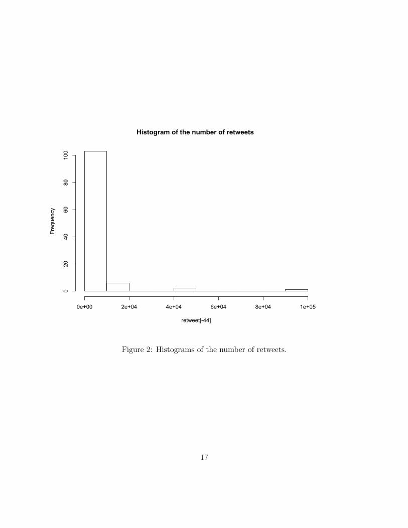
Table 2 describes our data in terms of total number of retweets produced by each tweet

account, and Figure 2 describes graphically the corresponding frequency distribution.

Table 2 about here

Figure 2 about here

10

From Figure 2 note that the distribution of the retweets is very right skewed. From

such distribution the main summary statistics assume the following values: mean=10610,

median=586, maximum=824600 and minimum=0.

Table 3 and Figure 3 reports, for the same data, the h-index of the different twitterers,

and the corresponding distribution.

Figure 3 about here

Table 3 about here

From Figure 3 note that the distribution of the h index is, as expected, similar to the

distribution of the retweets, but appears more concentrated: mean=19.02, median=9, max-

imum=505 and minimum=0. Indeed the skewness and kurtosis of the h index are 8.23 and

75.24. So far we have obtained a ranking measure of the tweets. We now move to a the con-

struction of confidence intervals, so to make a more accurate comparison between different

twitterers.

The distribution functions p(ni) and k(xi) will be estimated from our data that can be

thought as of a sample of twitterers assumed with common citation distribution Fi(x).

The observed sample correlation between the number of produced tweets and the total

retweet impact is equal to 0.95, and therefore we explore the case θi = θ ∗ ni, in addition to

the simpler assumption θi = θ.

To exemplify the methodology, we consider the application of what proposed to the

comparison of four twitterers. We considered either the Uniform-Poisson, the Uniform-fZM

and the Uniform-Negative Binomial convolutions to evaluate the most performing approaches

that can be different from the previous context since the citation vector is referred to a

specific twitterer. We have considered as running example, four twitterers: @mtaibbi with

an observed h index of 113 and 875 tweets, @PIMCO with an observed h index of 102

and 962 tweets, @ECONOMISTHULK with an observed h index of 48 and 782 tweets and

@justinwolfers with an observed h index of 48 and 371 tweets (all updated at February

2014). For each of them we have estimated the Uniform-Poisson and the Uniform-Negative

11

Binomials convolutions estimating the parameters on the relative retweet counts vectors.

It turns out that the parameters of the uniform distribution depend on the number of

tweets for each tweeterer: the mean number of tweets is equal to m = 45.83 (@mtaibbi),

m = 45.97 (@PIMCO), m = 13.54 (@ECONOMISTHULK), m = 24.43 (@justinwolfers).

On the other hand, the dispersion parameter is equal to d = 0.283 (@mtaibbi), d = 0.817

(@PIMCO), d = 0.120 (@ECONOMISTHULK) and d = 0.36 (@justinwolfers).

In order to quantify the real difference among the four tweeterer we can now calculate

the confidence intervals of their h index with level of confidence equal to 90%.

Table 4 shows the results.

Table 4 about here

From Table 4 the reader can infer that the Uniform-NB convolution contains the ob-

served h-index and moreover it is clearly shown that @mtaibbi and @PIMCO, even showing

different h index, are not significantly different between each other since their corresponding

confidence intervals overlap.

4 Conclusions

In this paper we have addressed the topic of evaluating the quality of tweet data taking

statistical variability into proper account. The well known Hirsch index (the h index) is

convincing, from a descriptive ranking perspective, but not from a stochastic viewpoint. We

overcome this problem by embedding the retweet counts, of which the h index is a function,

in an appropriate probability framework that takes inspiration from loss data modeling.

The resulting ’statistical h index’ can thus boost the descriptive power of the measure

proposed by Hirsch, not limiting it to summary purposes but allowing inferential evaluations,

such as confidence intervals. The added value of our proposal is not to rely on the large

sample distribution of the h index but to fully respect the discrete nature of the data by

deriving the exact distribution of the h index and proposing a discrete convolution model to

draw exact inferential conclusions.

12

From an applied perspective, we foresee at least two main advantages in the adoption of

our statistical h index:

1. comparison among twitterers can be simply performed in terms of easy to understand

ranking;

2. rankings can be robustified by using appropriate confidence intervals and levels.

Indeed our approach can be applied not only to retweets in Twitter but also to Likes in

Facebook and to similar social network measures, without loss of generality.

In general, our proposal can be profitably applied to all media contexts characterized by

two types of information that can be summarized by a random variable representing a count

frequency and a random variable representing the corresponding impact.

Finally, what developed can be obviously applied to the original bibliometric context

where the h-index was proposed (see, with this respect, Cerchiello and Giudici, 2013).

BIBLIOGRAPHY

Beirlant, J., and J. H. J. Einmahl, 2010, Asymptotics for the Hirsch Index: Scandinavian

Journal of Statistics, v. 37, p. 355-364.

Ball, P. 2005, Index aims for fair ranking of scientists, Nature, 436:900.

Burrell, Q. L., 2007, Hirsch’s h-index: A stochastic model: Journal of Informetrics, v. 1,

p. 16-25.

Cerchiello, P., and P. Giudici, 2012, On the distribution of functionals of discrete ordinal

variables: Statistics and Probability Letters, v. 82, p. 2044-2049.

Cerchiello, P., and P. Giudici, 2013, On a statistical H-index. To appear in Scientometrics.

Cruz M. G. 2002, ”Modeling, measuring and hedging operational risk.” Wiley.

Dalla Valle, L., and P. Giudici, 2008, A Bayesian approach to estimate the marginal loss

distributions in operational risk management: Computational Statistics and Data Analysis,

v. 52, p. 3107-3127.

13

Evert, S. 2004, A simple LNRE model for random character sequences. In Proceedings of

the 7mes Journes Internationales dAnalyse Statistique des Donnes Textuelles (JADT 2004),

pages 411422, Louvain-la-Neuve, Belgium

Evert, S. and Baroni, M. 2007, zipfR: Word frequency distributions in R. In Proceedings

of the 45th Annual Meeting of the Association for Computational Linguistics, Posters and

Demonstrations Session, Prague, Czech Republic.

Gabaix, X., 2009, Power Laws in Economics and Finance: Annual Review of Economics,

v. 1, p. 255-293.

Glanzel, W., 2006, On the h-index - A mathematical approach to a new measure of

publication activity and citation impact: Scientometrics, v. 67, p. 315-321.

Harzing, A.W. 2007 Publish or Perish, available from http://www.harzing.com/pop.htm

Hirsch, J. E., 2005, An index to quantify an individual’s scientific research output: Pro-

ceedings of the National Academy of Sciences of the United States of America, v. 102, p.

16569-16572.

Iglesias, J. E., and C. Pecharroman, 2007, Scaling the h-index for different scientific ISI

fields: Scientometrics, v. 73, p. 303-320.

Izsak, F., 2006, Maximum likelihood estimation for constrained parameters of multino-

mial distributions - Application to Zipf-Mandelbrot models: Computational Statistics and

Data Analysis, v. 51, p. 1575-1583.

King, D., Ramirez-Cano, D., Greaves, F., Vlaev, I., Beales, S., Darzi, A. (2013). Twitter

and the health reforms in the English national health service. Health policy 110, vol. 2-3.

Mandelbrot, B. 1962, On the theory of word frequencies and on related Markovian models

of discourse. In R. Jakobson (ed.), Structure of Language and its Mathematical Aspects,

pages 190219. American Mathematical Society, Providence, RI.

Pratelli, L., A. Baccini, L. Barabesi, and M. Marcheselli, 2012, Statistical Analysis of the

Hirsch Index: Scandinavian Journal of Statistics, v. 39, p. 681-694.

Todeschini, R., 2011, The j-index: a new bibliometric index and multivariate comparisons

between other common indices: Scientometrics, v. 87, p. 621-639.

14

Histogram of the number of tweets

tweet

Frequency

0 500 1000 1500 2000 2500 3000

020

4060

80

Figure 1: Histograms of the number of tweets.

15

Table 1: Number of tweets for each twitterer (arranged in alphabetical order) during the

year 2013.ID n. Tweets ID n. Tweets ID n. Tweets ID n. Tweets

@abnormalreturns 2263 @ECONOMISTHULK 782 @justinwolfers 371 @Queen Europe 1939

@AdamPosen 41 @economistmeg 36 @kathylienfx 286 @RedDogT3Live 1100

@alaidi 1431 @EpicureanDeal 398 @katie martin FX 438 @ReformedBroker 297

@Alea 121 @EU Eurostat 713 @KavanaghKillik 1278 @reinman mt 328

@alexmasterley 353 @EU Markt 82 @KeithMcCullough 273 @RencapMan 714

@andrealeadsom 141 @ezraklein 241 @LaMonicaBuzz 68 @RichardJMurphy 186

@andrewrsorkin 138 @FaullJonathan 31 @LaurenLaCapra 97 @ritholtz 461

@AngryArb 78 @felixsalmon 502 @Lavorgnanomics 1242 @robertjgardner 37

@Austan Goolsbee 10 @FGoria 295 @lemasabachthani 596 @SallieKrawcheck 71

@BergenCapital 1971 @finansakrobat 108 @LorcanRK 96 @Scaramucci 306

@bespokeinvest 2451 @firoozye 621 @mark dow 404 @ScottMinerd 362

@bill easterly 49 @footnoted 500 @MarkMobius 1001 @SEK bonds 2995

@bobivry 102 @Fullcarry 150 @MatinaStevis 114 @SharonBowlesMEP 303

@bondvigilantes 978 @GCGodfrey 1067 @mattyglesias 249 @Simon Nixon 88

@BrendaKelly IG 102 @greg ip 171 @MBarnierEU 263 @SimoneFoxman 71

@BritishInsurers 120 @GSElevator 1072 @michaelhewson 1 @SonyKapoor 2562

@chrisadamsmkts 36 @GTCost 300 @MorrisseyHelena 78 @stlouisfed 3000

@counterparties 207 @gusbaratta 55 @mtaibbi 875 @TedTobiasonDB 780

@CVecchioFX 152 @harmongreg 2019 @NicTrades 96 @TheBubbleBubble 387

@DanielAlpert 110 @hblodget 1286 @Nouriel 110 @TheNickLeeson 54

@danprimack 284 @hmtreasury 56 @OpenEurope 257 @TradeDesk Steve 1681

@DavidJones IG 0 @howardlindzon 146 @Pawelmorski 403 @Trader Dante 517

@davidmwessel 153 @Hugodixon 243 @pdacosta 151 @truemagic68 642

@DCBorthwick 289 @IvanTheK 2220 @pensionlawyeruk 779 @WillJAitken 239

@DKThomp 319 @jdportes 92 @PensionsMonkey 101 @WhelanKarl 277

@Dorte Hoppner 109 @Joe Trading 182 @petenajarian 518 @WilliamsonChris 128

@DougKass 414 @JohnKayFT 118 @PIMCO 962 @World First 220

@dsquareddigest 809 @JohnMannMP 107 @PIRCpress 381 @ZorTrades 331

@zerohedge 739

16

Histogram of the number of retweets

retweet[-44]

Frequency

0e+00 2e+04 4e+04 6e+04 8e+04 1e+05

020

4060

80100

Figure 2: Histograms of the number of retweets.

17

Table 2: Number of retweets for each twitterer (arranged in alphabetical order) during the

year 2013.ID n. Retweets ID n. Retweets ID n. Retweets ID n. Retweets
























@DCBorthwick 107 @IvanTheK 1215 @pensionlawyeruk 65 @WhelanKarl 554

@DKThomp 1683 @jdportes 157 @PensionsMonkey 105 @WilliamsonChris 601

@Dorte Hoppner 61 @Joe Trading 41 @petenajarian 758 @WillJAitken 109


@dsquareddigest 301 @JohnMannMP 799 @PIRCpress 199 @zerohedge 12534

@ZorTrades 202

18

Histogram of the h index on the tweets

h_tweets[-44]

Frequency

0 20 40 60 80 100 120 140

020

4060

80

Figure 3: Histograms of the h index for the tweetterer.

19

Table 3: H index of tweets for each twitterer (arranged in alphabetical order) during the

year 2013.ID h index ID h index ID h index ID h index
























@DCBorthwick 4 @IvanTheK 11 @pensionlawyeruk 3 @WhelanKarl 10

@DKThomp 19 @jdportes 7 @PensionsMonkey 5 @WilliamsonChris 12

@Dorte Hoppner 3 @Joe Trading 2 @petenajarian 12 @WillJAitken 3


@dsquareddigest 7 @JohnMannMP 13 @PIRCpress 4 @zerohedge 46

@ZorTrades 6

20

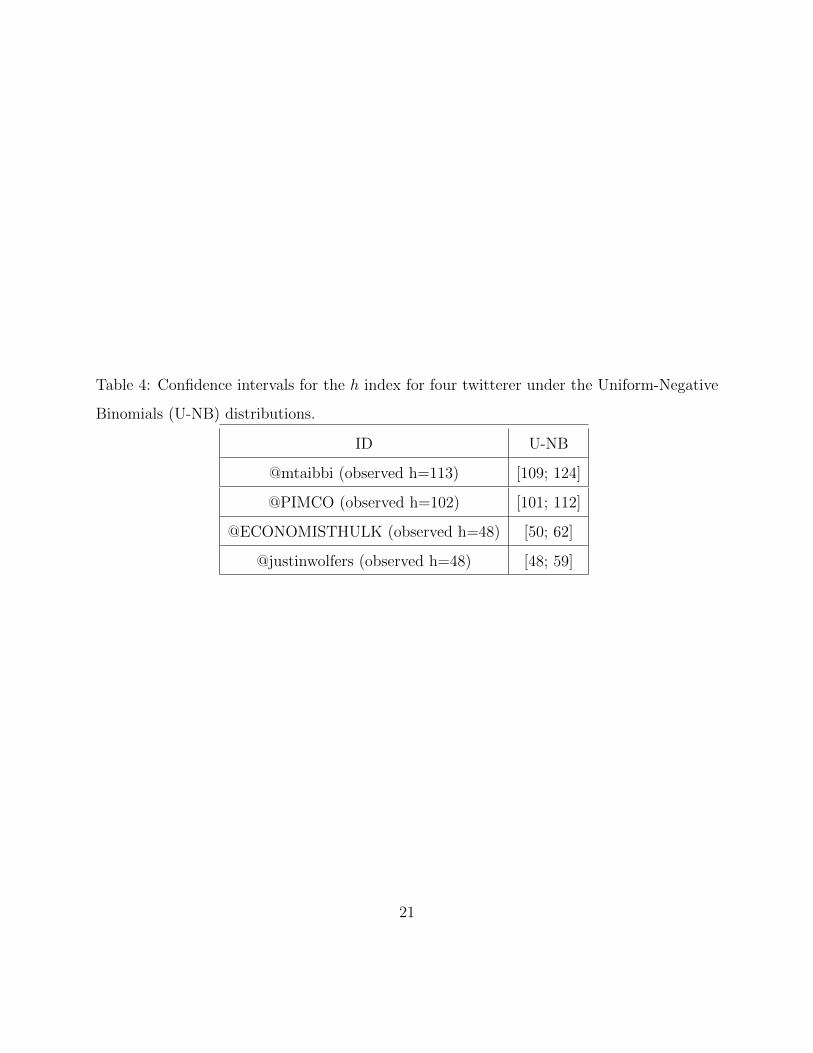
Table 4: Confidence intervals for the h index for four twitterer under the Uniform-Negative

Binomials (U-NB) distributions.

ID U-NB

@mtaibbi (observed h=113) [109; 124]

@PIMCO (observed h=102) [101; 112]

@ECONOMISTHULK (observed h=48) [50; 62]

@justinwolfers (observed h=48) [48; 59]

21

how to measure the quality of financial tweets paola

Documents