how to measure distance on a digital terrain surface and
TRANSCRIPT
Geographical Analysis (2020) 0 1ndash35
doi 101111gean12255 copy 2020 The Ohio State University
1
How to Measure Distance on a Digital Terrain Surface and Why it Matters in Geographical Analysis
Yi Qiang1 Barbara P Buttenfield2 Maxwell B Joseph3
1 Department of Geography and Environment University of Hawaii at Manoa Honolulu HI USA 2 Department of Geography University of Colorado at Boulder Boulder CO USA 3 Earth Lab University of Colorado at Boulder Boulder CO USA
Distance is the most fundamental metric in spatial analysis and modeling Planar distance and geodesic distance are the common distance measurements in current geographic information systems and geospatial analytic tools However there is little understanding about how to measure distance in a digital terrain surface and the uncertainty of the measurement To fill this gap this study applies a Monte-Carlo simulation to evaluate seven surface-adjustment methods for distance measurement in digital terrain model Using parallel computing techniques and a memory optimization method the processing time for the distances calculation of 6000 simulated transects has been reduced to a manageable level The accuracy and computational efficiency of the surface-adjustment methods were systematically compared in six study areas with various terrain types and in digital elevation models in different resolutions Major findings of this study indicate a trade-off between measurement accuracy and computational efficiency calculations at finer resolution DEMs improve measurement accuracy but increase processing times Among the methods compared the weighted average demonstrates highest accuracy and second fastest processing time Additionally the choice of surface adjustment method has a greater impact on the accuracy of distance measurements in rougher terrain
Introduction
Distance is a fundamental spatial metric which is used to measure route length travel distance feature size and shape and is also the foundation of higher-order spatial metrics such as area and volume Distance metrics provide a foundation for spatial analysis and modeling such as buffering pattern analysis spatial clustering shortest path analysis and geostatistical analysis The accuracy of distance measurement is of critical importance to many physical models such as flood inundation (Tucker and Hancock 2010) avalanche risk evaluation (Gutieacuterrez 2012) stream extraction (Stanislawski Falgout and Buttenfield 2015) regional power line routing
Correspondence Yi Qiang Department of Geography and Environment University of Hawaii at Manoa Saunders 416 2424 Maile Way Honolulu HI-96822 USAe-mail yiqianghawaiiedu
Submitted 12 August 2019 Revised version accepted 10 July 2020
Geographical Analysis
2
(Kiessling et al 2014) and analysis of surface pollutants such as nitrogen (Harms Wentz and Grimm 2009) all of which are commonly implemented in raster data models in order to register with terrain or imagery layers Currently planar distance and geodesic distance are the common surface distance metrics in geographic information systems (GIS) and geospatial analytic tools The former metric assumes the earth surface is a flat plane and distance is the length of the straight line from Location A to B The latter takes into account the curvature of the Earth and is used more often in longer distance measurements such as flight and shipping routes However neither of the two takes into account undulations and irregularities in topography which causes uncertainty in distance measurement on a terrain surface In this article we refer to distance that accounts for terrain irregularity as surface-adjusted distance Knowing how to accurately measure surface-adjusted distance is of critical importance for spatial models that are sensitive to distance measurement
Theoretically measuring distance on Light Detection and Ranging (LiDAR) data should generate the most precise measurement relative to coarser resolution terrain However the availability of LiDAR data is far from comprehensive in developed nations not to mention in rural and undeveloped regions Additionally storing rendering and processing large LiDAR point clouds can be computationally expensive which may not be applicable or necessary in national continental or global modeling tasks or in applications for which coarser resolution data are sufficient Instead measurement on coarser resolution digital elevation models (DEMs) which are formed by a regular spatial grid of elevation values provides a more practical solution for many analytical and modeling tasks An alternative data model forms a network of triangular facets (Triangulated Irregular Networks or TINs) that require more computation to generate but that characterize elevations at finer resolution where terrain is more rough or uneven DEMs are used more commonly in modeling tasks because they are faster to generate to process and to integrate with other data layers
Distance measurements on DEMs rely upon two assumptions adopted historically for prag-matic reasons relating to slower computational speeds and restricted data volumes One assump-tion is that the measured distance between points can be approximated by the distance between centroids of pixels containing such points Another assumption is that pixels are flat and rigid analogous to ceramic tiles Reliance upon these assumptions generates inaccurate and imprecise distance measures and we will demonstrate that these inaccuracies vary notably with changing pixel size In fact as pixel size increases it is less likely that a point lying within that pixel sits squarely on the centroid Moreover terrain can bend twist and undulate within each pixel With wide availability of faster computational speeds and High Performance Computing (HPC) this article argues that the two assumptions can and should be relaxed by accepting that observed points do not commonly fall directly on a pixel centroid and by accounting for slope and non-uniform terrain for any distance measured on a DEM
The process of surface adjustment relaxes the two assumptions To understand the distinc-tion between distance measured on rigid pixels as opposed to surface-adjusted pixels readers might consider the comparative analogy between measuring distance ldquoas the crow fliesrdquo and ldquoas the horse runsrdquo (Buttenfield et al 2016) The important questions to ask are first how much improvement in accuracy can be expected at a given spatial resolution (ie pixel size) and second what balance is achieved between the improved accuracy and additional computational cost required for surface adjustment These questions form the basis for the experiments reported in this article Answers to these questions establish a foundation for migrating GIS and spatial
Yi Qiang et al How to Measure Distance on a Digital Terrain Surface
3
analysis tools from the simplistic ldquoas the crow fliesrdquo paradigm to the more realistic ldquoas the horse runsrdquo paradigm
The analysis will gain novel insights to the effect of scale which are commonly acknowl-edged in geographical analysis (Qiang et al 2018 Qiang and Van de Weghe 2019) The ex-periment attempts to answer higher level questions such as (1) do finer resolution data always provide more accurate distance measurement (2) is there an operational scale where a geo-graphical phenomenon (eg a terrain surface in this case) can be modeled most accurately The impact of scale in terrain modeling have been reported in other studies For instance Usery et al (2004) assessed deviations in DEM elevations at varying resolutions and found that elevation values match well (R2 = 09) for DEM resolutions between 3 m and 30 m but gradually deviate as pixel sizes increase Chang and Tsai (1991) evaluated the effect of DEM resolution on slope and aspect estimation and found these two indices vary with resolution and landscape changes Kienzle (2004) conducted a comprehensive assessment of the effect of DEM resolution on a wider range of terrain indices including elevation slope aspect curvature and wetness index and showed an increasing root-mean-square error (RMSE) of these indices as the resolution coarsens Zhang and Montgomery (1994) assessed several topographic indices and found that 10 m grid size provides a substantial improvement over 30 m and 90 m data but 2 m or 4 m data provide only marginal additional improvement Moreover varying resolution can also influence the output of seismic models based on terrain analysis (Shafique et al 2011) All these studies demonstrate the importance of scale (or resolution) for spatial modeling in digital terrain models This article looks into the most basic spatial metric (ie distance) which lays a foundation to develop scale-sensitive spatial analysis tools for terrain modeling
Notwithstanding advances in data processing mentioned above distance measurement on digital terrain models has not been systematically assessed following logic that accuracy im-provements are so small that surface adjustment is unwarranted For individual pixels inaccura-cies may be small but additive effects can propagate dramatically especially in regional models (eg disaster evacuation) or global models (eg sea level rise) It is also uncertain how inaccu-racies propagate at different resolutions and in different types of terrain (eg smooth or rugged homogenous or heterogeneous) Estimating the within-pixel position of points and associated elevations can be accomplished using a variety of interpolation methods and these may con-tribute also to varying degrees of inaccuracy (Ghandehari 2019) As large-scale physical models become increasingly common especially for modeling regional and global environmental sys-tems compelling reasons emerge to develop surface-adjusted spatial metrics and understand the uncertainties of their accuracies in different conditions
Buttenfield et al (2016) conducted a pilot study to assess errors in distance measurement on six different DEMs at different resolutions The results show that the errors generally increase at coarser resolutions and results vary with different surface adjustment methods and in different landscapes (flat or hilly rough or smooth) Due to the computational cost of measuring distance on different DEMs and differing terrain conditions that pilot study was limited to the measure-ment of only five transects in each landscape This study extends that pilot study by using a Monte Carlo simulation to systematically evaluate a larger sample of 1000 transects per study area to quantify the effects of multiple variables (resolution surface adjustment method and ter-rain type) on distance measurement The computational challenge of this simulation is overcome by parallelizing the program into multiple computing units which reduces the total processing time to an acceptable range
Geographical Analysis
4
Data and study area
According to data availability and landscape diversity six study areas are selected for this study which are located in Louisiana (LA) Colorado (CO) North Carolina (NC) Nebraska (NE) Texas (TX) and Washington (WA) respectively Each study area is covered by a 3 m LiDAR DEM that will be used for the benchmark measurement and DEMs at 10 m 30 m 100 m and 1000 m resolutions which will be used for the analytic evaluation DEM areas range from 249116 km2 in Colorado to 778493 km2 in North Carolina
These study areas have diverse landscapes (see Fig 1 and Table 1) The CO study area is slim extending from north to south along the Arkansas River Valley with mountains to the east and west and a valley in the middle The WA study area covers the mountainous Skagit River valley and the flatter Skagit River delta which is relatively flat The study area in LA is flat in general with an elevation range from minus06 m to 688 m The area west of Mississippi River Channel is very flat while the terrain east of the river is slightly hilly with small rivers or creeks flowing from north to south The TX study area is flat located between Waco and Austin The NC study area extends from the eastern part of Appalachian Mountains to the Piedmont Plateau with an elevation range from 19259 m to 161697 m The NE study area has a homogeneous and hilly pattern carved by numerous streams and small drainage channels
The 3 m LiDAR DEMs were from the USGS National Elevation Dataset (NED) and were downloaded through The National Map (httpsviewernatio nalmapgovbasic) in 2016 By 2018 the NED DEMs were renamed 3DEP (3-Dimensional Elevation Program) seamless bare earth DEMs (Stoker personal communication 2018) The USGS NED has seamless raster eleva-tion data for the conterminous United States Alaska Hawaii US island territories Mexico and Canada The accuracy of NED varies spatially due to the diversity of data sources The overall absolute vertical accuracy of this dataset has an RMSE of 155 m based on the geodetic control points of the National Geodetic Survey (NGS) that have millimeter- to centimeter-level accura-cies (Gesch Oimoen and Evans 2014) This RMSE is equivalent to 304 m as assessed using the National Standard for Spatial Data Accuracy (NSSDA) at a 95 confidence level
The 10 m 30 m DEMs were downloaded from the Geospatial Data Gateway (httpsgdgscegovusdagov) The source for the 100 m and 1000 m DEMs was Shuttle Radar Topography Mission (SRTM) (httpddscrusgsgovsrtmversi on2_1) The absolute vertical accuracy of this dataset has an RMSE of 401 m (Gesch Oimoen and Evans 2014) The spatial reference systems of LA CO NC NE TX and WA are NAD1983 UTM Zone 13N 15N 17N 14N 14N and 10N respectively Data for all sources are independently compiled DEMs generated according to the methodology outlined in (Gesch 2007) It should be noted that the actual DEM resolutions are 19 13 1 3 and 30 arc-seconds with pixel sizes that are approximately 3 m 10 m 30 m 100 m and 1000 m respectively Source data for the DEM tiles are listed explicitly in the Appendix
Methods
One thousand random transects were created in each study area to a Monte Carlo approximation of all possible linear paths across each terrain surface The surface-adjusted lengths of these transects were estimated using different methods and applied to the six study areas in DEMs at four different resolutions of DEMs Surface-adjusted transect length measurements were com-pared with the benchmark distances measured on 3 m LiDAR DEMs using the closest centroid
Yi Qiang et al How to Measure Distance on a Digital Terrain Surface
5
Fig
ure
1 S
tudy
are
as (
figur
es m
odifi
ed f
rom
But
tenfi
eld
et a
l 2
016)
Geographical Analysis
6
method The deviation of the surface-adjusted distances from the benchmark distances in dif-ferent conditions was systematically evaluated to quantify and compare accuracies of a suite of surface-adjusted distance measurement methods The methodology of this study is described in more detail in the following sections
Transect generationA thousand random transects were created in each study area (eg Fig 2) The transect lengths were confined to range between 900 m (30 times of the cell size of the 3 m DEM) and the lon-ger edge of the bounding box of the study area (eg 84275 m for North Carolina) Confining lengths of transects into the same range will allow comparisons of results among the study areas As some study areas have an irregular boundary the 1000 transects were created in an iterative way First 1000 pairs of random points were created within the DEM boundary and linked to form 1000 transects Transects intersecting the DEM boundary or outside the length range were deleted The process was repeated generating another 1000 transects in the same way and delet-ing any transects intersecting the boundary or out of the length range The algorithm terminated when the set of valid transects contained 1000 or more paths from which 1000 transects were randomly selected for the simulation The same process was repeated creating 1000 transects for each of the six study areas resulting in 6000 transects in total These transects are stored as comma-delimited values (csv) files recording only the coordinates of their start and end points
Table 1 Information for the Study Areas Ranked on the Magnitude of Elevation Range
Study area Area Elevation range Landscape type DEM (10 m) size
Washington 453049 km2 minus07 to 23412 m Mountainous 424 MBColorado 249116 km2 21084ndash42259 m Mountainous 518 MBNorth Carolina 778493 km2 19259ndash16169 m Hilly 348 MBNebraska 470843 km2 6355ndash9375 m Hilly 226 MBTexas 547256 km2 1000ndash4688 m Flat 667 MBLouisiana 530568 km2 minus46 to 700 m Flat 243 MB
Figure 2 1000 transects created randomly in the study area of North Carolina
Yi Qiang et al How to Measure Distance on a Digital Terrain Surface
7
Surface-adjusted measurementsSeven surface-adjusted methods are evaluated in this study Five methods are based the DEM model and two are applied to the TIN model (Fig 3) All surface adjustments are based upon a sampling approach A certain number of points are randomly sampled along each transect The number of points is dependent on the length of transect and resolution of the DEM The point generation process is specifically detailed in Sections ldquoSurface-adjusted measurementsrdquo and ldquoSimulationrdquo below Elevations at the points are estimated using one of the seven methods de-scribed below Distances are then computed by summing transect segment lengths between ad-jacent pairs of sampled points The tested methods all incorporate elevation and slope and differ in estimation method and in contextual information about surrounding pixels or facets to gain a suite of surface-adjusted distance metrics The seven tested methods are described as follows
Methods for DEMClosest Centroid (clos) This method is based on a sampling approach A number of random points are sampled along the transect The elevation of each point is taken to be the elevation of the centroid of the pixel in which the sample point is located The overall length of a transect is the aggregation of distances between each pair of adjacent sample points The clos method is used to calculate the benchmark distance in the 3 m LiDAR DEMs
Weighted Average (wavg) This method follows the same sampling approach as for clos However the elevation of a sample point is estimated as the weighted average of the eight sur-rounding DEM pixels The total length of a transect is the aggregated distance between adjacent sample points
Polynomial Methods (3) Three polynomial methods estimate the elevations of sample points by fitting local polynomials within a specific neighborhood The Bilinear method (biLin) fits a first order polynomial using the four pixels nearest to the sample point The Biquadratic method (biQua) fits a second order equation to eight nearest pixels The Bicubic method (biCub) fits a third order polynomial using sixteen nearest pixels
Figure 3 Surface adjustment methods and neighborhoods in DEM and TIN data models
Geographical Analysis
8
Methods for TINTIN (TIN) This method first converts the DEM into a TIN and then interpolates the elevation of each sample point linearly from the three vertices of the triangular facet that contains it
Natural Neighbor (NN) This method (Sibson 1981) first converts the TIN centroids into Thiessen polygons Then the (off-centroid) sample points seed a second layer of Thiessen polygons The pro-portion of overlap between the two layers weights interpolation of the elevations of the sample points
SimulationThe distances along the 1000 transects in six study areas were measured using the seven surface adjustment methods and at four different resolutions The derived surface-adjusted distances were then compared with benchmark distances measured on 3 m LiDAR DEMs to evaluate accuracy For each transect the distance measurement used the seven surface adjustment methods and DEMs at four resolutions (10 m 30 m 100 m and 1000 m) Distance was measured by selecting points ran-domly along each transect and summing the lengths between adjacent point pairs For the LiDAR benchmark distances were measured using the clos method as described above thus summing distances between adjacent pixel centroids to give (on average) 3 m resolution Point sampling was thinned to preserve proportional sampling for the four test resolutions and to avoid oversampling To give a sense of the data volume involved in the simulation consider a perfectly situated east-west transect with a length of 90 km It would cover 30000 pixels at LiDAR resolution and have 30000 points sampled randomly along its length for the simulation Thinning to 10 m resolution would re-duce the sampling rate to select 9000 points randomly Likewise a random sample of 3000 points would be collected at 30 m and 900 points at 100 m and 90 points at 1000 m resolution
Using sequential programming the simulation could be implemented as a nested ldquofor looprdquo which calculated the distance for 1000 random transects per study area in DEMs at 4 resolu-tions using 7 methods and in 6 study areas The estimated processing time for the entire simula-tion would exceed 500 h (~21 days) The following pseudocode shows the sequential workflow and the number in the parentheses are the number of elements in each loop
for study_area in list_study_area (6)
for DEM in list_DEM (4)
for method in list_method (7)
for transect in list_Transect (study_area 1000)
DistCalc
Since distance calculations of the transects are independent the simulation can be parti-tioned into parallel tasks for simultaneous processing in multiple computing units Each com-puting unit calculates the distance of a transect using a specific surface adjustment method on a single DEM at a single resolution By doing so the simulation can be partitioned into 168000 (1000 transects times 4 DEMs times 7 methods times 6 study areas) independent processes which can theoretically complete the simulation in ~107 s if all processes are run concurrently As will be discussed in the results section average processing times ranged between roughly 5 s and more than 80 s for these DEMs at 10 m resolution depending on transect lengths
The simulation program is developed in Python using open-source spatial analysis pack-ages including numpy (Oliphant 2006) GDAL (GDALOGR contributors 2020) and natgrid (University Corporation for Atmospheric Research (UCAR) 2004) The open-source program is transferable across platforms and can be easily implemented in supercomputer clusters The
Yi Qiang et al How to Measure Distance on a Digital Terrain Surface
9
parallel computing uses the IPyparallel module (The IPython Development Team 2018) which is IPythonrsquos architecture for parallel and distributed computing The IPyparallel module sup-ports different modes of parallelism including Single Program Multiple Data (SPMD) paral-lelism Multiple Program Multiple Data (MPMD) parallelism and Message Passing Interface (MPI) The distance computations of transects in different conditions are compiled into a map function which simultaneously applies a function to lists of inputs and returns a list of outputs The IPyparallel module supports a parallel version of the map function which can dynamically balance the workload assigned to different processor cores The simulation program iteratively applies a distance calculation function to four lists of parameters which are transects study areas DEM resolutions and surface-adjusted methods The simulation was conducted with 16 times 32 GHz processor cores and 64 GB RAM The program can also run in Amazon Elastic Compute (EC2) Cloud cloud-based servers The simulation program for this study is shared in a GitHub repository (httpsgithubcomqiang -yisurfa ce_adjus ted_distance)
Create a LoadBalancedView object that dynamically balance workload to the computing
instances
lview = rcload_balanced_view()
Use a map function to execute the distance calculation for each transect method DEM
resolution and study area
distance = lviewmap(Calculation
cases_df[rsquotransectrsquo]tolist()
cases_df[rsquomethodrsquo]tolist()
cases_df[rsquoresolutionrsquo]tolist()
cases_df[rsquostudy_arearsquo]tolist())
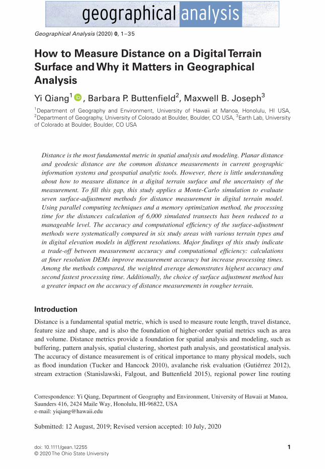
Memory control The location (ie the start and end coordinates) of the transect and the DEM raster are the inputs for surface-adjusted distance calculation in DEM (Fig 4a) To compute the distances of 1000 transects the DEM raster needs to be opened 1000 times in memory which can quickly exceed the RAM of a computing node For instance if the 10 m DEM of the smallest study area is opened 1000 times a total amount of 503 GB memory will be occupied which exceeds the total RAM of most computing nodes Also opening the entire DEM for a single transect is an unnecessary redundancy which may increase overhead when passing data across nodes To solve this problem
Figure 4 Converting the buffer area of a transect into a list of X-Y-Z tuples (a) the entire DEM (b) the DEM buffer in raster format (c) the DEM buffer in csv format
Geographical Analysis
10
a buffer is built around each transect and only the transects and buffer areas around them are sent into a distance computation Instead of storing the buffer areas in raster which still contain nu-merous no-data pixels within the Minimum Bounding Rectangle (eg Fig 4b) pixels inside the buffer areas are converted into X-Y-Z tuples which are stored in comma-separated values (csv) files (Fig 4c) By doing so the input data size for distance calculation of a transect can be reduced from gt 100 MB to ~1 MB The data conversion process introduces additional computational cost associated with the overhead of generating csv files for each path However the smaller DEM buffers increase the efficiency of distance computation by reducing computational overhead of data transfer to and from the computing nodes and reducing overall memory requirements
Results
Distances calculated using different surface adjustment methods on DEMs of different resolu-tions are compared with the benchmark distance measured at 3 m LiDAR data using the Closest Centroid method Residuals and Root-Mean-Square Error (RMSE) metrics between the mea-sured distances and benchmark distances evaluate the measurement accuracy Processing times of distance measurement are also compared to evaluate the computational efficiency of the different interpolation methods
Residual analysisResiduals indicate discrepancies between the measured distances and benchmark distances in the simulated transects (ie measured distancemdashbenchmark distance) Fig 5 shows that the residuals of most methods (except closest centroids) are negative at finest resolutions indicat-ing underestimation but at coarser resolutions approaching zero or becoming positive As an exception the closest centroid (clos) method overestimates distances at finer resolutions and transitions to underestimation as pixel size increases Magnitude of residuals for this method is highest IN most situations except the 1000 m resolution where the residuals of the various methods converge The weighted average (wavg) residuals are generally closer to zero than all other methods while the TIN and Natural Neighbor methods have the largest negative residu-als Comparing the three polynomial methods the residuals of the bilinear method most closely approximate the benchmark (ie lowest absolute residuals) followed by the biquadratic and bicubic methods Thus the increasing complexity of the polynomial function actually reduces accuracy of distance measurement likely due to overfitting
Maximum residual values are higher for more mountainous and hilly landscapes and the mag-nitude of errors appears to relate as much or more to terrain roughness (ie elevation range as shown in Table 1) as to DEM size Washington is roughly the same size as Nebraska and yet con-tains much larger residuals Colorado is not even half the size of Louisiana and yet its residuals are larger by orders of magnitude Working across spatial resolutions the progression of residual values generated by all methods differs most strongly at 10 m and then resolves as pixel size increases to 1000 m Residuals for the three flattest terrains tend to converge at 100 m resolution diverging by 10ndash20 m as overestimation becomes evident for 1000 m pixels This finding possibly implies that variations in accuracy of the different interpolation methods relates to terrain flatness or perhaps to terrain uniformity Confirmation of this would require further characterization of the DEM surfaces
The simulated transects vary in length and the residuals are highly dependent on the tran-sect length To eliminate the effect of transect length ratios of the residuals by transect lengths were calculated to compare the measurement accuracy per distance unit Fig 6 shows that the
Yi Qiang et al How to Measure Distance on a Digital Terrain Surface
11
Fig
ure
5 M
ean
resi
dual
s (m
easu
red
in m
eter
s) b
etw
een
mea
sure
d di
stan
ces
and
benc
hmar
k di
stan
ces
at d
iffe
rent
res
olut
ions
Pos
itive
val
ues
refle
ct
over
-est
imat
ion
and
nega
tive
valu
es re
flect
und
er-e
stim
atio
n re
lativ
e to
the
LiD
AR
dat
a T
he y
-axe
s ar
e lin
ear a
nd v
ary
amon
g D
EM
s a
nd th
e x-
axes
ar
e ex
pone
ntia
l and
iden
tical
For
any
par
ticul
ar lo
catio
n an
d re
solu
tion
met
hods
with
line
s cl
oses
t to
zero
on
the
y-ax
is a
re m
ore
accu
rate
on
aver
age
Geographical Analysis
12
Fig
ure
6 M
ean
resi
dual
rat
ios
betw
een
benc
hmar
k di
stan
ces
and
mea
sure
d di
stan
ces
mea
sure
d at
dif
fere
nt r
esol
utio
ns P
ositi
ve v
alue
s re
flect
ove
r-es
timat
ion
and
nega
tive
valu
es r
eflec
t und
er-e
stim
atio
n r
elat
ive
to th
e L
iDA
R d
ata
Not
e th
at th
e y-
axes
dif
fer
acro
ss D
EM
s w
hile
the
x-ax
es a
re
cons
iste
nt a
nd lo
gari
thm
ical
ly r
esca
led
Yi Qiang et al How to Measure Distance on a Digital Terrain Surface
13
changing pattern of the ratios of residuals at different resolutions are analogous to the patterns of residuals shown in Fig 5 As shown in Fig 6 the error ratio of distance measurement for any given transect may range from minus2 to +4 depending on the surface-adjusted method the study area and on the resolution of the DEM Comparing among the study areas Louisiana has the smallest error magnitude with residual ratios ranging from ndash01 to 03 while the residual ratios in Colorado span ranging from minus02 to 27 indicating that distance measurement error tends to be larger in mountainous or uneven terrains than in flatter or smoother terrains
RMSE analysisRoot-Mean-Square Error (RMSE) indicates the absolute fit between measured distances and benchmark distances The RMSEs in Fig 7 generally confirm the patterns of residuals in Figs 5 and 6 with some interesting cross scale patterns highlighted RMSE values tend to rise as pixel size increases from 100 m with RMSE increasing for North Carolina and Colorado for 30 m and larger pixels Method-specific errors show greatest differences at finer resolutions resolv-ing to a value ranging between roughly 450 m (Nebraska) and 600 m (all other study areas) at 1000 m resolution The range of average error among methods is higher for mountainous and hilly landscapes with almost no difference among methods for the two flattest landscapes (Texas and Louisiana) The Weighted Average method generates the lowest RMSE magnitudes overall although the Closest Centroid method gives lower RMSE values at 100 m resolution for reasons that are not clear The bilinear method has the lowest RMSE of all three polynomial methods followed by the biquadratic and bicubic method
Processing timeProcessing time of the distance calculation increases at finer resolutions (ie as cell size de-creases) (Fig 8) TIN and Nearest Neighbor require the longest processing times except for North Carolina at 10 m resolution Shortest processing times are used by Weighted Average and Closest Centroid followed by the bilinear polynomial Processing times drop considerably for coarser resolution DEMs because of relatively fewer pixels Considering the changing patterns of residuals and RMSEs however there is a trade-off between accuracy and computational efficiency
Comparing among the different methods the Natural Neighbor and TIN method require the longest processing time in most landscapes Given their high residuals and RMSEs these two methods seem the least optimal for surface-adjusted distance calculation And while the Closest Centroid method takes the shortest processing time the accuracy metrics indicate that its utility for surface-adjusted distance estimation is highly varied and thus not consistently reliable The bilinear polynomial method gives more accurate estimations but takes additional processing time especially at fine resolutions Given the low absolute residuals and RMSEs in most landscapes and at most resolutions the weighted average method can be considered the sur-face adjusting method that best balances accuracy with processing time for distance calculation
Discussion and implications
This study applies a HPC-enabled Monte-Carlo simulation to evaluate seven surface adjustment methods for distance calculation on digital terrain Distances of 1000 randomly generated tran-sects were calculated in six study areas using different surface adjusting methods and DEMs at different resolutions The calculated distances were compared with benchmark distances
Geographical Analysis
14
Fig
ure
7 R
MSE
(m
easu
red
in m
eter
s) b
etw
een
benc
hmar
k di
stan
ces
and
mea
sure
d di
stan
ces
mea
sure
d in
dif
fere
nt r
esol
utio
ns N
ote
that
the
y-ax
es
are
scal
ed d
iffe
rent
ly a
cros
s pa
nels
Yi Qiang et al How to Measure Distance on a Digital Terrain Surface
15
Fig
ure
8 M
ean
proc
essi
ng ti
mes
(mea
sure
d in
sec
onds
) for
sur
face
-adj
uste
d di
stan
ce c
alcu
latio
n pe
r tra
nsec
t usi
ng d
iffe
rent
met
hods
and
at d
iffe
rent
re
solu
tions
Not
e th
at y
-axi
s va
lues
dif
fer
amon
g D
EM
s w
hile
x-a
xis
valu
es a
re id
entic
al
Geographical Analysis
16
measured on 3 m resolution DEMs to evaluate their accuracies Residuals and RMSEs compared measured distances with LiDAR benchmark distances To reduce the overall computing time the distance calculation algorithm was optimized to reduce memory usage and processing time in a multi-core computer
The major findings in this study include (1) the distance measurement varies with DEM res-olutions surface adjustment methods and terrain types (2) Weighted Average is overall the most accurate surface adjustment for distance measurement with a few exceptions (3) there is a trade-off between DEM resolution and computing time The assessment results provide a foundation for distance-based spatial analyses on terrain surface (eg distance-based point pattern analysis and kriging interpolation) In a broader sense the study increases the understanding about the interplay between analytic methods scale and the geographical phenomena being studied
The assessment reveals the dependency of distance measurement on data resolution surface adjustment methods and terrain variations The results show a pattern of distance underestimation relative to the LiDAR benchmarks at finer resolutions (10 m and 30 m) that transitions to near equivalence or slight overestimation as pixel size increases The degree of underestimation varies with method of surface adjustment The weighted average method has the highest accuracy overall in most situations This finding may seem surprising given that the method utilizes a search neigh-borhood of only 8 adjacent pixels In terrain with high local relief one might expect that the polyno-mial methods would provide better results due to larger neighborhoods andor adjustment methods that could filter localized perturbations in elevation The results indicate that biquadratic (8 neigh-bors) and the bicubic (16 neighbors) methods tend to exaggerate underestimation While the bilinear neighborhood (4 pixels) produces residuals and RMSE values closer to the weighted average the kernel is rarely centered on the point being adjusted and this can over- or underemphasize nearby terrain nonuniformity Closest Centroid TIN and Nearest Neighbor employ even smaller neighbor-hoods (1 3 and up to 6 neighbors respectively) further exacerbating the problem Overestimation of surface-adjusted distance for all methods at 1000 m resolution may be associated with neigh-borhood bias as well the spatial extent of larger pixels may ignore local features at the same time as weighting more distant features (up to 4 8 or 16 kilometers away) in equal consideration The weighted average method adjustment is based on central tendency and qualified by inverse distance weighting which can offset the impacts of rough or uneven terrain in more distant pixels
The balance between improved accuracy and extra processing time is relevant from a prac-tical standpoint The DEMs tested here are probably too small to be useful for regional or conti-nental modeling as for example studies involving sea level rise earthquake damage or coastal storm events Even with high performance computing distance adjustment for larger study areas could require minutes or longer Moreover distance estimation is often the initial step and rarely the final product of spatial modeling The Closest Centroid method calculates distance based on elevation in rigid pixels which does not adjust the terrain surface using surrounding elevation values Thus the distance measurements of this method fluctuate at different resolutions due to the stair-step effect of DEM pixels As a consequence the method tends to over-estimate distance at finer resolutions due to including too many (small) pixels and to under-estimate distance at coarser resolutions due to averaging within large pixels Despite carrying the lowest processing time the accuracy of the Closest Centroid method should not be considered a good choice when trying to balance accuracy with processing times Higher processing times shown by TIN and Nearest Neighbor are coupled with reduced accuracy and no balance is achieved Polynomial adjustment by second and third order equations reflects similar results Given the second lowest processing time the weighted average method can be considered the optimal surface adjusting
Yi Qiang et al How to Measure Distance on a Digital Terrain Surface
17
method for distance calculation in most situations Adjustment using bilinear polynomial estima-tion can be considered an alternative with slightly less improvement in accuracy
The accuracy of the surface adjustment methods also varies in different terrain types The ac-curacy difference among methods is smallest in flat terrain such as Louisiana and Texas implying that for these terrain types the choice of surface adjustment for distance measurements matters less than for hilly and mountainous terrain Differences in error metrics for more mountainous or nonuniform terrains show greater variation especially at fine and intermediate resolutions mean-ing the choice of surface adjustment appears to have a greater impact on distance estimation in rougher terrain and at finer resolutions Error magnitudes begin to coalesce after 100 m resolution for all methods indicating that at some point the extra computations required for surface adjust-ment are simply not worth the potential improvement in accuracy Accuracy of surface-adjusted distance measurement is reduced in DEMs that contain a mix of terrain types with some flat and some hilly areas Future research must investigate the relationships between terrain roughness terrain uniformity and accuracy to better understand the full implication of these findings
As an additional note methods that perform best for distance calculation may or may not be optimal for other tasks such as estimating surface-adjusted elevation or area Ghandehari Buttenfield and Farmer (2019) demonstrate that linear and bilinear polynomials give slightly better accuracies for surface-adjusted estimation of point elevation on DEMs although errors for any method are quite small on the order of centimeter magnitudes for terrain measured in me-ters Their study shows however that errors for all methods increase in rough terrain This reflects earlier research by Shi and Tian (2006) and Schneider (2001) showing that errors in elevation estimation are more prominent in rough terrain Ghandehari and Buttenfield (2018) compare sur-face-adjusted methods for estimating pixel surface areas finding that while a bicubic polynomial estimation gives the highest accuracy relative to a 3 m LiDAR benchmark it carries unreason-ably high processing times They modify Jennessrsquo (2004) surface area estimation method and then apply bilinear polynomial estimation to achieve nearly equivalent accuracies to the bicubic method with processing times reduced by nearly 80 (Ghandehari 2019)
As the primary objective of the study is to evaluate and compare among surface adjustment methods the simulation program is implemented in a simple parallel model which effectively reduces the computing time to a manageable level The performance of the simulation can be further improved with finer grain parallelism architectures such as OpenMP and MPI Also the program can be further parallelized by including on-the-fly transect generation and buffer area extraction These optimization options will be explored in future experiments such as surface-ad-justed area calculation for a new variety of case studies
The title of this article raises the issue of why accurate distance measurements matters in geographical analysis There are several reasons First and as described at the beginning of the article distance metrics underlie many if not most simple and compound GIS analytic methods Second it stands to reason that inaccurate distances can propagate inaccuracies throughout the entire course of spatial modeling and confound any estimates related to terrain surfaces as for ex-ample glacial recession wetlands fragmentation freight routing or debris flow estimation Third digital terrain is one of the most frequently included data layers in spatial analyses Bolstad (2019 p 485) cites the influence of terrain characteristics on a broad set of environmental functions such as soil moisture agricultural yields sediment transport and construction costs Wilson (2012 p 107) explains the important impact of terrain ldquohellip in modulating the atmospheric geomor-phic hydrologic and ecological processes operating on or near the Earthrsquos surfacerdquo He refers to Hutchinson and Gallant (2000) in arguing that the terrain is so tightly coupled with these four
Geographical Analysis
18
families of processes that characterization of the terrain directly leads to and refines insights about the nature of the processes In a nutshell geospatial analytics cannot be accurate without accurate distance metrics And because most geographic and geomorphic processes depend partially or wholly upon the land surface on which they are situated distance measurements should be per-formed on the terrain surface ldquoas the horse runsrdquo instead of ldquoas the crow fliesrdquo
With the emergence of parallel processing and the increased availability of fine resolution terrain data surface-adjusted distance metrics are becoming an operational strategy that can improve the accuracy of many types of spatial modeling although results depend upon several factors (resolution terrain type and uniformity and surface adjustment method) Three of those factors have been examined here but this study has limitations that call for additional examina-tion and assessment The characterization of terrain uniformity must be examined more formally along with possible interaction among the factors analyzed in this article Additionally the opti-mal methods choices need to be further tested and validated by embedding the surface-adjusted distance metrics into more complex analytics For instance a hypothesis to be tested is whether surface-adjusted distance can increase the accuracy of kriging interpolation Surface adjustment also needs to be embedded in full-blown surface process models to understand them in analytic practice And finally the assessment of distance measurement shows that choosing an appropri-ate (not necessarily the finest) scale is important for spatial analysis and modeling Quattrochi and Goodchild (1997) suggest that geographical analyses should be conducted at the operational scale (also referred to by Montello (2001) as phenomenon scale) where the studied processes operate since slight changes in these processes can invoke pronounced changes in model results The results reported in this study reveal that the optimal DEM resolutions for distance mea-surement varies among different surface adjustment methods and terrain types Importantly the choice of a method may also depend upon task (measuring distance surface area or volume) As distance is the most fundamental metric for geographical analyses the knowledge generated in this study lays a foundation for developing scale-sensitive analysis tools on a terrain surface
Acknowledgment
The authors acknowledge excellent and constructive comments from reviewers which strength-ened the text
Funding information
This article is based on work supported by the US National Science under the Methodology Measurement amp Stats (MMS) Program (Award No 1853866) This article is also based on work that is part of the Data Harmonization Initiative at Earth Lab (httpswwwcolor adoeduearth lab) supported by an investment from the University of Colorado Grand Challenge Initiative Any opinions findings and conclusions or recommendations expressed in this material are those of the authors and do not necessarily reflect the views of the funding agencies
Appendix
This appendix documents the data sets and their download sources used for the experiments in the manuscript The exact specifications are included here in the interests of reproducible sci-ence so that interested readers can replicate the study using the same data sets
Yi Qiang et al How to Measure Distance on a Digital Terrain Surface
19
Benchmark LiDAR data
State Benchmark LiDAR datasets
Colorado 2010 South San Luis Lakes LidarNebraska 2009 Nebraska Department of Natural Resources (DNR) South Central
Nebraska LidarNorth Carolina 2003 North Carolina Floodplain Mapping Program (NCFMP) LidarTexas 2011 Texas Natural Resources Information System (TNRIS) Lidar Bell
Burnet and McLennan CountiesWashington 2006 USGS Lidar North Puget Sound WashingtonLouisiana 1999 Louisiana Lidar Project (1999ndash2008)
Tiles of 10 m DEMsThe following tiles are available to download in USGS TNM Download httpsviewernatio nalmapgovbasic
State Tiles of 10 m DEM
Colorado USGS NED ned19_n39x25_w106x25_co_arkansasvalley_2010 19 arc-second 2012 15 times 15 min IMGUSGS NED ned19_n39x00_w106x50_co_arkansasvalley_2010 19 arc-second 2012 15 times 15 min IMGUSGS NED ned19_n38x75_w106x00_co_arkansasvalley_2010 19 arc-second 2012 15 times 15 min IMGUSGS NED ned19_n39x50_w106x00_co_grandco_2010 19 arc-second 2011 15 times 15 min IMGUSGS NED ned19_n38x75_w106x50_co_arkansasvalley_2010 19 arc-second 2012 15 times 15 min IMGUSGS NED ned19_n38x25_w106x25_co_sanluisvalley_2011 19 arc-second 2012 15 times 15 min IMGUSGS NED ned19_n38x50_w106x00_co_arkansasvalley_2010 19 arc-second 2012 15 times 15 min IMGUSGS NED ned19_n38x25_w106x00_co_arkansasvalley_2010 19 arc-second 2012 15 times 15 min IMGUSGS NED ned19_n38x25_w106x25_co_arkansasvalley_2 010 19 arc-second 2012 15 times 15 min IMGUSGS NED ned19_n39x25_w106x50_co_arkansasvalley_2010 19 arc-second 2012 15 times 15 min IMGUSGS NED ned19_n38x25_w106x00_co_sanluisvalley_2011 19 arc-second 2012 15 times 15 min IMGUSGS NED ned19_n39x00_w106x00_co_arkansasvalley_2010 19 arc-second 2012 15 times 15 min IMGUSGS NED ned19_n39x50_w106x25_co_arkansasvalley_2010 19 arc-second 2012 15 times 15 min IMGUSGS NED ned19_n38x50_w106x25_co_arkansasvalley_2010 19 arc-second 2012 15 times 15 min IMGUSGS NED ned19_n38x25_w106x50_co_sanluisvalley_2011 19 arc-second 2012 15 times 15 min IMG
Geographical Analysis
20
State Tiles of 10 m DEM
USGS NED ned19_n39x50_w106x50_co_arkansasvalley_2010 19 arc-second 2012 15 times 15 min IMGUSGS NED ned19_n38x75_w106x25_co_arkansasvalley_2010 19 arc-second 2012 15 times 15 min IMGUSGS NED ned19_n39x00_w106x25_co_arkansasvalley_2010 19 arc-second 2012 15 times 15 min IMGUSGS NED ned19_n38x25_w105x75_co_sanluisvalley_2011 19 arc-second 2012 15 times 15 min IMGUSGS NED ned19_n39x75_w106x00_co_grandco_2010 19 arc-second 2011 15 times 15 min IMGUSGS NED ned19_n38x00_w106x25_co_sanluisvalley_2011 19 arc-second 2012 15 times 15 min IMGUSGS NED ned19_n38x00_w106x00_co_sanluisvalley_2011 19 arc-second 2012 15 times 15 min IMGUSGS NED ned19_n38x00_w106x50_co_sanluisvalley_2011 19 arc-second 2012 15 times 15 min IMGUSGS NED ned19_n38x00_w105x75_co_sanluisvalley_2011 19 arc-second 2012 15 times 15 min IMG
Nebraska USGS NED ned19_n40x50_w100x25_ne_rainwater_2009 19 arc-second 2011 15 times 15 min IMGUSGS NED ned19_n40x50_w100x00_ne_rainwater_2009 19 arc-second 2011 15 times 15 min IMGUSGS NED ned19_n40x50_w100x50_ne_rainwater_2009 19 arc-second 2011 15 times 15 min IMGUSGS NED ned19_n40x75_w100x75_ne_rainwater_2009 19 arc-second 2011 15 times 15 min IMGUSGS NED ned19_n40x75_w100x00_ne_rainwater_2009 19 arc-second 2011 15 times 15 min IMGUSGS NED ned19_n40x75_w100x25_ne_rainwater_2009 19 arc-second 2011 15 times 15 min IMGUSGS NED ned19_n40x75_w100x50_ne_rainwater_2009 19 arc-second 2011 15 times 15 min IMGUSGS NED ned19_n40x50_w100x75_ne_rainwater_2009 19 arc-second 2011 15 times 15 min IMGUSGS NED ned19_n40x75_w101x00_ne_rainwater_2009 19 arc-second 2011 15 times 15 min IMGUSGS NED ned19_n40x50_w101x00_ne_rainwater_2009 19 arc-second 2011 15 times 15 min IMGUSGS NED ned19_n40x25_w100x00_ne_rainwater_2009 19 arc-second 2011 15 times 15 min IMGUSGS NED ned19_n40x25_w100x50_ne_rainwater_2009 19 arc-second 2011 15 times 15 min IMGUSGS NED ned19_n40x25_w100x25_ne_rainwater_2009 19 arc-second 2011 15 times 15 min IMG
Yi Qiang et al How to Measure Distance on a Digital Terrain Surface
21
State Tiles of 10 m DEM
USGS NED ned19_n40x25_w100x75_ne_rainwater_2009 19 arc-second 2011 15 times 15 min IMGUSGS NED ned19_n41x00_w100x75_ne_rainwater_2009 19 arc-second 2011 15 times 15 min IMGUSGS NED ned19_n41x00_w100x00_ne_rainwater_2009 19 arc-second 2011 15 times 15 min IMGUSGS NED ned19_n41x00_w100x50_ne_rainwater_2009 19 arc-second 2011 15 times 15 min IMGUSGS NED ned19_n41x00_w100x25_ne_rainwater_2009 19 arc-second 2011 15 times 15 min IMGUSGS NED ned19_n40x75_w099x75_ne_rainwater_2009 19 arc-second 2011 15 times 15 min IMGUSGS NED ned19_n40x50_w099x75_ne_rainwater_2009 19 arc-second 2011 15 times 15 min IMGUSGS NED ned19_n40x25_w101x00_ne_rainwater_2009 19 arc-second 2011 15 times 15 min IMGUSGS NED ned19_n41x00_w101x00_ne_rainwater_2009 19 arc-second 2011 15 times 15 min IMGUSGS NED ned19_n40x25_w099x75_ne_rainwater_2009 19 arc-second 2011 15 times 15 min IMGUSGS NED ned19_n41x00_w099x75_ne_rainwater_2009 19 arc-second 2011 15 times 15 min IMG
North Carolina
USGS NED ned19_n36x00_w081x50_nc_statewide_2003 19 arc-second 2012 15 times 15 min IMGUSGS NED ned19_n36x00_w082x00_nc_statewide_2003 19 arc-second 2012 15 times 15 min IMGUSGS NED ned19_n36x00_w081x25_nc_statewide_2003 19 arc-second 2012 15 times 15 min IMGUSGS NED ned19_n36x00_w081x75_nc_statewide_2003 19 arc-second 2012 15 times 15 min IMGUSGS NED ned19_n36x00_w081x00_nc_statewide_2003 19 arc-second 2012 15 times 15 min IMGUSGS NED ned19_n36x00_w082x25_nc_statewide_2003 19 arc-second 2012 15 times 15 min IMGUSGS NED ned19_n35x75_w082x00_nc_statewide_2003 19 arc-second 2012 15 times 15 min IMGUSGS NED ned19_n35x75_w081x25_nc_statewide_2003 19 arc-second 2012 15 times 15 min IMGUSGS NED ned19_n35x75_w081x50_nc_statewide_2003 19 arc-second 2012 15 times 15 min IMGUSGS NED ned19_n35x75_w081x75_nc_statewide_2003 19 arc-second 2012 15 times 15 min IMGUSGS NED ned19_n35x75_w081x00_nc_statewide_2003 19 arc-second 2012 15 times 15 min IMG
Geographical Analysis
22
State Tiles of 10 m DEM
USGS NED ned19_n35x75_w082x25_nc_statewide_2003 19 arc-second 2012 15 times 15 min IMGUSGS NED ned19_n36x25_w081x50_nc_statewide_2003 19 arc-second 2012 15 times 15 min IMGUSGS NED ned19_n36x25_w081x00_nc_statewide_2003 19 arc-second 2012 15 times 15 min IMGUSGS NED ned19_n36x25_w081x25_nc_statewide_2003 19 arc-second 2012 15 times 15 min IMGUSGS NED ned19_n36x25_w082x00_nc_statewide_2003 19 arc-second 2012 15 times 15 min IMGUSGS NED ned19_n36x25_w081x75_nc_statewide_2003 19 arc-second 2012 15 times 15 min IMGUSGS NED ned19_n36x25_w082x25_nc_statewide_2003 19 arc-second 2012 15 times 15 min IMGUSGS NED ned19_n36x00_w080x75_nc_statewide_2003 19 arc-second 2012 15 times 15 min IMGUSGS NED ned19_n35x75_w080x75_nc_statewide_2003 19 arc-second 2012 15 times 15 min IMGUSGS NED ned19_n36x25_w080x75_nc_statewide_2003 19 arc-second 2012 15 times 15 min IMG
Texas USGS NED ned19_n31x50_w097x50_tx_bellburnetmclennancos_2011 19 arc-second 2012 15 times 15 min IMGUSGS NED ned19_n31x25_w097x25_tx_bellburnetmclennancos_2011 19 arc-second 2012 15 times 15 min IMGUSGS NED ned19_n31x00_w098x25_tx_bellburnetmclennancos_2011 19 arc-second 2012 15 times 15 min IMGUSGS NED ned19_n31x25_w097x50_tx_bellburnetmclennancos_2011 19 arc-second 2012 15 times 15 min IMGUSGS NED ned19_n31x50_w097x75_tx_bellburnetmclennancos_2011 19 arc-second 2012 15 times 15 min IMGUSGS NED ned19_n31x75_w097x25_tx_bellburnetmclennancos_2011 19 arc-second 2012 15 times 15 min IMGUSGS NED ned19_n31x25_w098x25_tx_bellburnetmclennancos_2011 19 arc-second 2012 15 times 15 min IMGUSGS NED ned19_n31x00_w098x00_tx_bellburnetmclennancos_2011 19 arc-second 2012 15 timestimes 15 min IMGUSGS NED ned19_n31x25_w097x75_tx_bellburnetmclennancos_2011 19 arc-second 2012 15 times 15 min IMGUSGS NED ned19_n31x00_w097x50_tx_bellburnetmclennancos_2011 19 arc-second 2012 15 times 15 min IMGUSGS NED ned19_n31x00_w097x75_tx_bellburnetmclennancos_2011 19 arc-second 2012 15 times 15 min IMGUSGS NED ned19_n31x75_w097x50_tx_bellburnetmclennancos_2011 19 arc-second 2012 15 times 15 min IMG
Yi Qiang et al How to Measure Distance on a Digital Terrain Surface
23
State Tiles of 10 m DEM
USGS NED ned19_n31x25_w098x00_tx_bellburnetmclennancos_2011 19 arc-second 2012 15 times 15 min IMGUSGS NED ned19_n31x00_w097x25_tx_bellburnetmclennancos_2011 19 arc-second 2012 15 times 15 min IMGUSGS NED ned19_n31x50_w097x25_tx_bellburnetmclennancos_2011 19 arc-second 2012 15 times 15 min IMGUSGS NED ned19_n30x75_w098x25_tx_bellburnetmclennancos_2011 19 arc-second 2012 15 times 15 min IMGUSGS NED ned19_n30x75_w098x00_tx_bellburnetmclennancos_2011 19 arc-second 2012 15 times 15 min IMGUSGS NED ned19_n30x75_w097x50_tx_bellburnetmclennancos_2011 19 arc-second 2012 15 times 15 min IMGUSGS NED ned19_n30x75_w098x00_tx_central_llano_2007 19 arc-second 2010 15 times 15 min IMGUSGS NED ned19_n30x75_w098x25_tx_central_llano_2007 19 arc-second 2010 15 times 15 min IMGUSGS NED ned19_n31x75_w097x00_tx_bellburnetmclennancos_2011 19 arc-second 2012 15 times 15 min IMGUSGS NED ned19_n31x50_w097x00_tx_bellburnetmclennancos_2011 19 arc-second 2012 15 times 15 min IMGUSGS NED ned19_n31x25_w098x50_tx_central_llano_2007 19 arc-second 2010 15 times 15 min IMGUSGS NED ned19_n31x50_w098x50_tx_central_llano_2007 19 arc-second 2010 15 times 15 min IMGUSGS NED ned19_n31x00_w098x50_tx_central_llano_2007 19 arc-second 2010 15 times 15 min IMGUSGS NED ned19_n31x75_w098x50_tx_central_llano_2007 19 arc-second 2010 15 times 15 min IMGUSGS NED ned19_n31x00_w098x50_tx_bellburnetmclennancos_2011 19 arc-second 2012 15 times 15 min IMGUSGS NED ned19_n30x75_w098x50_tx_central_llano_2007 19 arc-second 2010 15 times 15 min IMGUSGS NED ned19_n30x75_w098x50_tx_bellburnetmclennancos_2011 19 arc-second 2012 15 times 15 min IMG
Washington USGS NED ned19_n48x50_w122x00_wa_northpugetsound_2006 19 arc-second 2009 15 times 15 min IMGUSGS NED ned19_n48x50_w122x50_wa_puget_sound_2000 19 arc-second 2012 15 times 15 min IMGUSGS NED ned19_n48x50_w121x50_wa_northpugetsound_2006 19 arc-second 2009 15 times 15 min IMGUSGS NED ned19_n49x00_w122x50_wa_northpugetsound_2006 19 arc-second 2009 15 times 15 min IMGUSGS NED ned19_n48x75_w122x75_wa_sanjuanco_2009 19 arc-second 2011 15 times 15 min IMG
Geographical Analysis
24
State Tiles of 10 m DEM
USGS NED ned19_n48x50_w122x25_wa_northpugetsound_2006 19 arc-second 2009 15 times 15 min IMGUSGS NED ned19_n48x75_w121x25_wa_northpugetsound_2006 19 arc-second 2009 15 times 15 min IMGUSGS NED ned19_n49x00_w121x25_wa_northpugetsound_2006 19 arc-second 2009 15 times 15 min IMGUSGS NED ned19_n49x00_w122x00_wa_northpugetsound_2006 19 arc-second 2009 15 times 15 min IMGUSGS NED ned19_n48x50_w122x75_wa_puget_sound_2000 19 arc-second 2012 15 times 15 min IMGUSGS NED ned19_n48x75_w122x00_wa_northpugetsound_2006 19 arc-second 2009 15 times 15 min IMGUSGS NED ned19_n48x75_w122x75_wa_northpugetsound_2006 19 arc-second 2009 15 times 15 min IMGUSGS NED ned19_n48x75_w121x75_wa_northpugetsound_2006 19 arc-second 2009 15 times 15 min IMGUSGS NED ned19_n48x75_w122x25_wa_northpugetsound_2006 19 arc-second 2009 15 times 15 min IMGUSGS NED ned19_n49x00_w121x75_wa_northpugetsound_2006 19 arc-second 2009 15 times 15 min IMGUSGS NED ned19_n48x75_w122x50_wa_northpugetsound_2006 19 arc-second 2009 15 times 15 min IMGUSGS NED ned19_n49x00_w122x25_wa_northpugetsound_2006 19 arc-second 2009 15 times 15 min IMGUSGS NED ned19_n48x50_w122x50_wa_northpugetsound_2006 19 arc-second 2009 15 times 15 min IMGUSGS NED ned19_n48x50_w122x75_wa_northpugetsound_2006 19 arc-second 2009 15 times 15 min IMGUSGS NED ned19_n48x75_w121x50_wa_northpugetsound_2006 19 arc-second 2009 15 times 15 min IMGUSGS NED ned19_n49x00_w122x75_wa_northpugetsound_2006 19 arc-second 2009 15 times 15 min IMGUSGS NED ned19_n48x50_w121x75_wa_northpugetsound_2006 19 arc-second 2009 15 times 15 min IMGUSGS NED ned19_n49x25_w122x25_wa_northpugetsound_2006 19 arc-second 2009 15 times 15 min IMGUSGS NED ned19_n49x25_w122x50_wa_northpugetsound_2006 19 arc-second 2009 15 times 15 min IMGUSGS NED ned19_n49x25_w122x00_wa_northpugetsound_2006 19 arc-second 2009 15 times 15 min IMGUSGS NED ned19_n49x25_w122x75_wa_northpugetsound_2006 19 arc-second 2009 15 times 15 min IMGUSGS NED ned19_n48x25_w122x50_wa_puget_sound_2000 19 arc-second 2012 15 times 15 min IMG
Yi Qiang et al How to Measure Distance on a Digital Terrain Surface
25
State Tiles of 10 m DEM
USGS NED ned19_n48x25_w122x75_wa_puget_sound_2000 19 arc-second 2012 15 times 15 min IMGUSGS NED ned19_n48x50_w123x00_wa_puget_sound_2000 19 arc-second 2012 15 times 15 min IMGUSGS NED ned19_n48x75_w123x00_wa_sanjuanco_2009 19 arc-second 2011 15 times 15 min IMGUSGS NED ned19_n49x00_w123x00_wa_northpugetsound_2006 19 arc-second 2009 15 times 15 min IMGUSGS NED ned19_n48x50_w123x00_wa_sanjuanco_2009 19 arc-second 2011 15 times 15 min IMGUSGS NED ned19_n49x25_w123x00_wa_northpugetsound_2006 19 arc-second 2009 15 times 15 min IMGUSGS NED ned19_n48x25_w123x00_wa_puget_sound_2000 19 arc-second 2012 15 times 15 min IMG
Louisiana USGS NED ned19_n30x75_w091x50_la_statewide_2006 19 arc-second 2009 15 times 15 min IMGUSGS NED ned19_n30x50_w091x00_la_statewide_2006 19 arc-second 2009 15 times 15 min IMGUSGS NED ned19_n30x50_w091x50_la_atchafalayabasin_2010 19 arc-second 2011 15 times 15 min IMGUSGS NED ned19_n30x50_w091x50_la_statewide_2006 19 arc-second 2009 15 times 15 min IMGUSGS NED ned19_n30x75_w091x00_la_statewide_2006 19 arc-second 2009 15 times 15 min IMGUSGS NED ned19_n30x75_w091x25_la_statewide_2006 19 arc-second 2009 15 times 15 min IMGUSGS NED ned19_n30x75_w090x75_la_statewide_2006 19 arc-second 2009 15 times 15 min IMGUSGS NED ned19_n30x50_w091x25_la_statewide_2006 19 arc-second 2009 15 times 15 min IMGUSGS NED ned19_n30x50_w090x75_la_statewide_2006 19 arc-second 2009 15 times 15 min IMGUSGS NED ned19_n30x50_w091x50_LA-USGS_Atchafalaya2_2012_2014 19 arc-second 20140615 15 15 min IMGUSGS NED ned19_n31x00_w091x50_la_statewide_2006 19 arc-second 2009 15 times 15 min IMGUSGS NED ned19_n31x00_w091x25_la_statewide_2006 19 arc-second 2009 15 times 15 min IMGUSGS NED ned19_n31x00_w091x00_la_statewide_2006 19 arc-second 2009 15 times 15 min IMGUSGS NED ned19_n31x00_w090x75_la_statewide_2006 19 arc-second 2009 15 times 15 min IMGUSGS NED ned19_n30x25_w091x00_la_statewide_2006 19 arc-second 2009 15 times 15 min IMG
Geographical Analysis
26
State Tiles of 10 m DEM
USGS NED ned19_n30x25_w091x50_la_atchafalayabasin_2010 19 arc-second 2011 15 times 15 min IMGUSGS NED ned19_n30x25_w091x50_la_statewide_2006 19 arc-second 2009 15 times 15 min IMGUSGS NED ned19_n30x25_w090x75_la_statewide_2006 19 arc-second 2009 15 times 15 min IMGUSGS NED ned19_n30x25_w091x25_la_statewide_2006 19 arc-second 2009 15 times 15 min IMGUSGS NED ned19_n30x25_w091x50_LA-USGS_Atchafalaya2_2012_2014 19 arc-second 20140615 15 times 15 min IMGUSGS NED ned19_n30x25_w091x25_LA-USGS_Atchafalaya2_2012_2014 19 arc-second 20140615 15 times 15 min IMGUSGS NED ned19_n30x75_w090x50_la_statewide_2006 19 arc-second 2009 15 times 15 min IMGUSGS NED ned19_n30x50_w090x50_la_statewide_2006 19 arc-second 2009 15 times 15 min IMGUSGS NED ned19_n30x75_w091x75_la_statewide_2006 19 arc-second 2009 15 times 15 min IMGUSGS NED ned19_n30x50_w091x75_la_atchafalayabasin_2010 19 arc-second 2011 15 times 15 min IMGUSGS NED ned19_n30x50_w091x75_la_statewide_2006 19 arc-second 2009 15 times 15 min IMGUSGS NED ned19_n30x75_w091x75_la_atchafalayabasin_2010 19 arc-second 2011 15 times 15 min IMGUSGS NED ned19_n30x75_w091x75_LA-USGS_Atchafalaya2_2012_2014 19 arc-second 20140615 15 times 15 min IMGUSGS NED ned19_n30x50_w091x75_LA-USGS_Atchafalaya2_2012_2014 19 arc-second 20140615 15 times 15 min IMGUSGS NED ned19_n31x00_w090x50_la_statewide_2006 19 arc-second 2009 15 times 15 min IMGUSGS NED ned19_n30x25_w090x50_la_statewide_2006 19 arc-second 2009 15 times 15 min IMGUSGS NED ned19_n31x00_w091x75_la_statewide_2006 19 arc-second 2009 15 times 15 min IMGUSGS NED ned19_n31x00_w091x75_LA-USGS_Atchafalaya2_2012_2014 19 arc-second 20140615 15 times 15 min IMGUSGS NED ned19_n30x25_w091x75_la_atchafalayabasin_2010 19 arc-second 2011 15 times 15 min IMGUSGS NED ned19_n30x25_w091x75_la_statewide_2006 19 arc-second 2009 15 times 15 min IMGUSGS NED ned19_n30x25_w091x75_LA-USGS_Atchafalaya2_2012_2014 19 arc-second 20140615 15 times 15 min IMG
Tiles of 30 m DEMs
Yi Qiang et al How to Measure Distance on a Digital Terrain Surface
27
The following tiles are available to download in USGS TNM Download httpsviewernatio nalmapgovbasic
State Tiles of 30 m DEM
Colorado USGS NED 13 arc-second n40w107USGS NED n39w107 13 arc-secondUSGS NED 13 arc-second n40w106USGS NED 13 arc-second n39w106
Nebraska USGS NED 13 arc-second n41w101 1 x 1 degree ArcGrid 2019USGS NED 13 arc-second n41w100 1 x 1 degree ArcGrid 2019
North Carolina USGS NED 13 arc-second n36w082 1 x 1 degree ArcGrid 2019USGS NED n36w081 13 arc-second 2013 1 x 1 degree ArcGridUSGS NED 13 arc-second n36w083 1 x 1 degree ArcGrid 2017USGS NED 13 arc-second n37w082 1 x 1 degree ArcGrid 2019USGS NED 13 arc-second n37w081 1 x 1 degree ArcGrid 2018USGS NED 13 arc-second n37w083 1 x 1 degree ArcGrid 2018
Texas USGS NED 13 arc-second n32w098 1 x 1 degree ArcGrid 2019USGS NED 13 arc-second n31w098 1 x 1 degree ArcGrid 2019USGS NED 13 arc-second n32w099 1 x 1 degree ArcGrid 2019USGS NED 13 arc-second n31w099 1 x 1 degree ArcGrid 2019USGS NED 13 arc-second n32w097 1 x 1 degree ArcGrid 2019USGS NED 13 arc-second n31w097 1 x 1 degree ArcGrid 2019
Washington USGS NED 13 arc-second n49w122 1 x 1 degree ArcGrid 2018USGS NED 13 arc-second n49w123 1 x 1 degree ArcGrid 2019USGS NED 13 arc-second n50w122 1 x 1 degree ArcGrid 2018USGS NED 13 arc-second n49w121 1 x 1 degree ArcGrid 2018USGS NED 13 arc-second n50w123 1 x 1 degree ArcGrid 2018
Louisiana USGS NED 13 arc-second n31w091 1 x 1 degree ArcGrid 2019USGS NED 13 arc-second n31w092 1 x 1 degree ArcGrid 2019
Tiles of 100 m and 1000 m DEMsThe following tiles are available to download in USGSrsquos website httpsddscrusgsgovsrtmversi on2_1
States Tiles 100 m DEM Tiles 1000 m DEM
Colorado N38W107SRTMGL3 w140n40SRTM30N39W107SRTMGL3N39W106SRTMGL3N38W106SRTMGL3
Nebraska N40W100SRTMGL3 w140n90SRTM30N40W101SRTMGL3
North Carolina N35W082SRTMGL3 w140n90SRTM30N35W081SRTMGL3N35W083SRTMGL3
Texas N29W098SRTMGL3N29W099SRTMGL3
Washington N48W123SRTMGL3 w100n40SRTM30N48W122SRTMGL3
Louisiana N29W091SRTMGL3 w100n40SRTM30N29W092SRTMGL3
Geographical Analysis
28
Tab
les
of
the
anal
ysis
res
ult
s
Tab
le A
1 R
esid
ual
Ave
rage
Res
idua
l R
MSE
and
Pro
cess
ing
Tim
e fo
r W
ashi
ngto
n I
nter
pola
tion
Met
hods
Inc
lude
(in
Top
-to-
Bot
tom
Ord
er)
Bic
ubic
Bili
near
and
Biq
uadr
atic
pol
ynom
ials
Clo
sest
Cen
troi
d N
eare
st N
eigh
bor
Tri
angu
late
d Ir
regu
lar
Net
wor
k a
nd W
eigh
ted
Ave
rage
Res
olut
ion
Stud
y ar
eaIn
terp
olat
ion
met
hod
Avg
res
idua
l (m
)A
vg t
ime
(s)
Avg
rat
io o
f re
sidu
alR
MSE
(m
)
10W
ashi
ngto
nbi
Cub
minus474
29
231
60minus0
016
0859
825
10W
ashi
ngto
nbi
Lin
minus275
87
210
59minus0
009
4235
463
10W
ashi
ngto
nbi
Qua
minus350
39
216
51minus0
011
9144
494
10W
ashi
ngto
ncl
os1
317
0319
142
004
514
166
534
10W
ashi
ngto
nN
Nminus8
785
922
620
minus00
2975
110
814
10W
ashi
ngto
nT
INminus7
763
841
305
minus00
2623
975
0410
Was
hing
ton
wav
g37
99
196
900
0013
599
64
30W
ashi
ngto
nbi
Cub
minus319
35
200
4minus0
010
8939
954
30W
ashi
ngto
nbi
Lin
minus136
67
117
3minus0
004
7117
310
30W
ashi
ngto
nbi
Qua
minus210
48
143
0minus0
007
1726
271
30W
ashi
ngto
ncl
os1
069
140
817
003
723
137
121
30W
ashi
ngto
nN
Nminus5
671
85
546
minus00
1943
722
4030
Was
hing
ton
TIN
minus476
51
113
48minus0
016
1159
879
30W
ashi
ngto
nw
avg
745
10
865
000
269
130
6510
0W
ashi
ngto
nbi
Cub
minus306
76
050
3minus0
010
5040
213
100
Was
hing
ton
biL
inminus1
754
80
273
minus00
0599
237
1110
0W
ashi
ngto
nbi
Qua
minus217
31
034
0minus0
007
2829
031
100
Was
hing
ton
clos
698
930
204
002
469
915
6410
0W
ashi
ngto
nN
Nminus4
112
01
650
minus00
1399
532
3210
0W
ashi
ngto
nT
INminus3
183
73
383
minus00
1065
416
4110
0W
ashi
ngto
nw
avg
minus22
260
201
minus00
0032
111
771
000
Was
hing
ton
biC
ubminus2
395
00
108
minus00
0719
548
591
000
Was
hing
ton
biL
inminus2
007
10
077
minus00
0754
516
001
000
Was
hing
ton
biQ
uaminus2
225
70
083
minus00
0850
543
431
000
Was
hing
ton
clos
299
990
068
001
204
578
811
000
Was
hing
ton
NN
minus223
18
014
7minus0
007
6052
918
100
0W
ashi
ngto
nT
INminus1
614
80
450
minus00
0758
471
211
000
Was
hing
ton
wav
gminus1
298
90
068
minus00
0484
496
20
Yi Qiang et al How to Measure Distance on a Digital Terrain Surface
29
Table A2 Residual Average Residual RMSE and Processing Time for North Carolina Interpolation Methods Include (in Top-to-Bottom Order) Bicubic Bilinear and Biquadratic polynomials Closest Centroid Nearest Neighbor Triangulated Irregular Network and Weighted Average
Resolution Study Area MethodAvg residual Avg time
Avg ratio of residual RMSE
10 North Carolina biCub minus39280 82186 minus000973 4971710 North Carolina biLin minus25592 78635 minus000643 3262710 North Carolina biQua minus30551 79250 minus000761 3872610 North Carolina clos 103191 75460 002535 13173110 North Carolina NN minus79594 34227 minus001958 10150610 North Carolina TIN minus75426 72281 minus001853 9519210 North Carolina wavg minus886 76333 minus000033 715030 North Carolina biCub minus36234 4078 minus000897 4675230 North Carolina biLin minus18032 2678 minus000452 2319130 North Carolina biQua minus25272 3131 minus000626 3251230 North Carolina clos 79456 1949 001972 10139030 North Carolina NN minus54725 10186 minus001360 7172030 North Carolina TIN minus52388 20687 minus001293 6667230 North Carolina wavg minus3793 2088 minus000093 6429100 North Carolina biCub minus38245 0921 minus000938 50519100 North Carolina biLin minus30836 0499 minus000754 40788100 North Carolina biQua minus33905 0624 minus000835 44764100 North Carolina clos 9981 0357 000278 19506100 North Carolina NN minus41975 2560 minus001046 55973100 North Carolina TIN minus39808 5935 minus000986 52072100 North Carolina wavg minus25205 0364 minus000618 330921000 North Carolina biCub minus13916 0122 minus000105 641361000 North Carolina biLin minus10973 0091 minus000167 623531000 North Carolina biQua minus14067 0096 minus000124 643461000 North Carolina clos minus5074 0083 minus000054 610341000 North Carolina NN minus14628 0120 minus000200 639841000 North Carolina TIN minus12287 0468 minus000255 623091000 North Carolina wavg minus13194 0081 minus000080 63061
Geographical Analysis
30
Table A3 Residual Average Residual RMSE and Processing Time for Colorado Interpolation Methods Include (in Top-to-Bottom Order) Bicubic Bilinear and Biquadratic Polynomials Closest Centroid Nearest Neighbor Triangulated Irregular Network and Weighted Average
Resolution Study Area Method Avg residual Avg timeAvg ratio of residual RMSE
10 Colorado biCub minus21068 7957 minus000968 2870810 Colorado biLin minus11997 5588 minus000566 1680410 Colorado biQua minus15591 6381 minus000729 2153010 Colorado clos 60424 4200 002749 7803210 Colorado NN minus35698 17031 minus001629 5060910 Colorado TIN minus42632 29384 minus001930 5665410 Colorado wavg 1410 4499 000046 585530 Colorado biCub minus18084 1800 minus000808 2462830 Colorado biLin minus8422 1095 minus000382 1198230 Colorado biQua minus12450 1309 minus000560 1721130 Colorado clos 45183 0729 002082 5887330 Colorado NN minus26450 3091 minus001182 3729630 Colorado TIN minus29240 7784 minus001326 3921530 Colorado wavg minus513 0798 minus000020 5506100 Colorado biCub minus18886 0520 minus000839 25817100 Colorado biLin minus13441 0311 minus000593 18908100 Colorado biQua minus15535 0367 minus000703 21444100 Colorado clos 16414 0208 000757 24211100 Colorado NN minus19998 0736 minus000922 28223100 Colorado TIN minus21186 2349 minus000992 28612100 Colorado wavg minus9335 0226 minus000413 143081000 Colorado biCub minus9685 0077 minus000350 630701000 Colorado biLin minus6277 0059 000636 633641000 Colorado biQua minus6457 0061 000222 586041000 Colorado clos minus911 0054 000077 597911000 Colorado NN minus9166 0078 000324 599841000 Colorado TIN minus8685 0234 minus000152 590841000 Colorado wavg minus3811 0054 000378 57750
Yi Qiang et al How to Measure Distance on a Digital Terrain Surface
31
Table A4 Residual Average Residual RMSE and Processing Time for Nebraska Interpolation Methods Include (in Top-to-Bottom Order) Bicubic Bilinear and Biquadratic polynomials Closest Centroid Nearest Neighbor Triangulated Irregular Network and Weighted Average
Resolution Study Area Method Avg residual Avg timeAvg ratio of residual RMSE
10 Nebraska biCub minus15507 15751 minus000438 1842310 Nebraska biLin minus8786 12139 minus000249 1051610 Nebraska biQua minus11645 13238 minus000329 1385010 Nebraska clos 36339 9779 001024 4281710 Nebraska NN minus24660 15574 minus000693 2919010 Nebraska TIN minus24193 35472 minus000681 2859210 Nebraska wavg minus1845 10406 minus000054 285030 Nebraska biCub minus12290 2861 minus000345 1480730 Nebraska biLin minus6632 1831 minus000187 812330 Nebraska biQua minus9544 2162 minus000269 1150730 Nebraska clos 23939 1287 000676 2831630 Nebraska NN minus15898 4681 minus000447 1896130 Nebraska TIN minus15391 10863 minus000436 1831230 Nebraska wavg minus3888 1374 minus000111 5014100 Nebraska biCub minus9337 0776 minus000268 12040100 Nebraska biLin minus7733 0470 minus000222 10434100 Nebraska biQua minus8326 0560 minus000232 11135100 Nebraska clos 1640 0330 000043 5837100 Nebraska NN minus10137 1126 minus000282 13097100 Nebraska TIN minus9717 3289 minus000271 12620100 Nebraska wavg minus6860 0341 minus000198 97011000 Nebraska biCub minus599 0131 000065 443391000 Nebraska biLin minus846 0090 000058 457281000 Nebraska biQua minus715 0098 000009 426081000 Nebraska clos 070 0076 minus000046 439671000 Nebraska NN minus2165 0120 minus000030 448871000 Nebraska TIN 049 0437 000077 452231000 Nebraska wavg minus658 0077 minus000055 44366
Geographical Analysis
32
Table A5 Residual Average Residual RMSE and Processing Time for Texas Interpolation Methods Include (in Top-to-Bottom Order) Bicubic Bilinear and Biquadratic Polynomials Closest Centroid Nearest Neighbor Triangulated Irregular Network and Weighted Average
Resolution Study Area Method Avg residual Avg timeAvg ratio of residual RMSE
10 Texas biCub minus6678 13527 minus000195 814210 Texas biLin minus4630 10210 minus000135 567810 Texas biQua minus5603 11303 minus000164 682910 Texas clos 10990 8228 000317 1408710 Texas NN minus9274 16384 minus000269 1155410 Texas TIN minus9619 34548 minus000280 1183410 Texas wavg minus2283 8734 minus000067 291030 Texas biCub minus4288 2730 minus000129 552930 Texas biLin minus2693 1761 minus000087 364330 Texas biQua minus3388 2076 minus000098 444730 Texas clos 7699 1241 000218 1039430 Texas NN minus5702 3433 minus000171 735530 Texas TIN minus5518 9743 minus000169 704430 Texas wavg minus1467 1330 minus000047 2510100 Texas biCub minus3155 0775 minus000107 6498100 Texas biLin minus2425 0481 minus000080 6196100 Texas biQua minus2945 0565 minus000079 6493100 Texas clos 4061 0338 000099 7431100 Texas NN minus3677 0815 minus000113 7056100 Texas TIN minus3622 3066 minus000121 7066100 Texas wavg minus1931 0355 minus000081 59641000 Texas biCub 929 0106 000991 601131000 Texas biLin 195 0078 001138 613451000 Texas biQua 870 0082 001353 622861000 Texas clos 220 0069 000922 616651000 Texas NN 2542 0097 000987 610911000 Texas TIN minus1579 0339 000748 633421000 Texas wavg minus218 0069 000829 61030
Yi Qiang et al How to Measure Distance on a Digital Terrain Surface
33
Table A6 Residual Average Residual RMSE and Processing Time for Louisiana Interpolation Methods Include (in top-to-bottom order) Bicubic Bilinear and Biquadratic polynomials Closest Centroid Nearest Neighbor Triangulated Irregular Network and Weighted Average
Resolution Study Area Method Avg residual Avg timeAvg ratio of residual RMSE
10 Louisiana biCub minus3132 25881 minus000084 384410 Louisiana biLin minus2262 22476 minus000061 279310 Louisiana biQua minus2722 23573 minus000073 334310 Louisiana clos 2551 19252 000070 318010 Louisiana NN minus3294 27879 minus000088 402610 Louisiana TIN minus3380 51336 minus000091 411510 Louisiana wavg minus1800 20357 minus000048 222330 Louisiana biCub minus1636 2924 minus000048 257630 Louisiana biLin minus1284 1806 minus000036 220030 Louisiana biQua minus1501 2171 minus000042 248230 Louisiana clos 486 1288 000013 175630 Louisiana NN minus1645 7183 minus000045 258830 Louisiana TIN minus1642 14367 minus000046 256330 Louisiana wavg minus1154 1367 minus000030 2129100 Louisiana biCub minus706 0792 minus000014 5329100 Louisiana biLin minus818 0492 minus000019 5458100 Louisiana biQua minus532 0579 minus000017 5348100 Louisiana clos minus543 0330 minus000003 5361100 Louisiana NN minus789 0772 minus000020 5375100 Louisiana TIN minus916 3179 minus000025 5644100 Louisiana wavg minus640 0361 minus000009 55851000 Louisiana biCub 494 0109 000265 584241000 Louisiana biLin 1730 0079 000215 593021000 Louisiana biQua 839 0084 000325 613951000 Louisiana clos 744 0067 000203 603861000 Louisiana NN minus119 0112 000123 602791000 Louisiana TIN 1416 0369 000168 599011000 Louisiana wavg 1211 0070 000236 59514
Geographical Analysis
34
References
Bolstad P (2019) GIS Fundamentals A First Text on Geographic Information systems 6th ed Ann Arbor MI XanEdu Publishing Inc
Buttenfield B M Ghandehari S Leyk L Stanislawski M Brantley Y Qiang (2016) Measuring Distance ldquoAs the Horse Runsrdquo Cross-Scale Comparison of Terrain-Based Metrics International Conference on GIScience Short Paper Proceedings 1 httpdxdoiorg1021433 b3118 rh987cz
Chang K and B Tsai (1991) ldquoThe Effect of DEM Resolution on Slope and Aspect Mappingrdquo Cartography and Geographic Information Systems 18(1) 69ndash77 httpsdoiorg10155915230 40917 83805626
GDALOGR contributors (2020) GDALOGR GEOSPATIAL Data Abstraction Software Library Open Source Geospatial Foundation httpsgdalorg
Gesch D B (2007) ldquoThe National Elevation Datasetrdquo In Digital Elevation Model Technologies and Applications The DEM Users Manual 2nd ed 99ndash118
Gesch DB M J Oimoen and G A Evans (2014) ldquoAccuracy Assessment of the US Geological Survey National Elevation Dataset and Comparison with Other Large-Area Elevation Datasets SRTM and ASTERrdquo Report No 2014ndash1008 Open-File Report p 18 USGS Publications Warehouse httpsdoiorg103133ofr20 141008
Ghandehari M (2019) Cross-Scale Analysis of Surface-Adjusted Measurements in digital Elevation Models Doctoral dissertation University of Colorado Boulder
Ghandehari M and B Buttenfield (2018) ldquoSlope-Adjusted Surface Area Computations in Digital Terrainrdquo Proceedings of 5th International Conference of the International Society of Geomorphometry (Geomorphometry 2018)
Ghandehari M B P Buttenfield C J Q Farmer (2019) Comparing the accuracy of estimated terrain elevations across spatial resolution International Journal of Remote Sensing 40(13) 5025ndash5049 httpdxdoiorg10108001431 16120191577581
Gutieacuterrez M (2012) ldquoChapter 153 Applied Geomorphology in Periglacial Reginsrdquo In Geomorphology 601ndash13 Boca Raton FL Taylor amp Francis
Harms T K E A Wentz and N B Grimm (2009) ldquoSpatial Heterogeneity of Denitrification in Semi-Arid Floodplainsrdquo Ecosystems 12(1) 129ndash43 httpsdoiorg101007s1002 1-008-9212-6
Hutchinson M F and J C Gallant (2000) Digital Elevation Models and Representation of Terrain Shape httpspubli catio nscsiroaurprpublist=BROamppid=proci te46f1d e5d-172e-4f8e-8696-da3b6 f7b03ca
Jenness J S (2004) ldquoCalculating Landscape Surface Area from Digital Elevation Modelsrdquo Wildlife Society Bulletin 32(3) 829ndash39 httpsdoiorg1021930091-7648(2004)032[0829CLSAF D]20CO2
Kienzle S (2004) ldquoThe Effect of DEM Raster Resolution on First Order Second Order and Compound Terrain Derivativesrdquo Transactions in GIS 8(1) 83ndash111 httpsdoiorg101111j1467-9671200400169x
Kiessling F P Nefzger J Nolasco and U Kaintzyk (2014) Overhead Power Lines Planning Design Construction Berlin Germany Springer
Montello D R (2001) ldquoScale in Geographyrdquo In International Encyclopedia of the Social and Behavioral Sciences 13501ndash4 edited by N J Smelser and B Baltes
Oliphant T E (2006) A guide to NumPy (Vol 1) Trelgol Publishing USAQiang Y B P Buttenfield N Lam and N V de Weghe (2018) ldquoNovel Models for Multi-Scale Spatial
and Temporal Analysesrdquo In 10th International Conference on Geographic Information Science (GIScience 2018) Vol 114 551ndash557 edited by S Winter A Griffin amp M Sester Dagstuhl Germany Schloss DagstuhlndashLeibniz-Zentrum fuer Informatik httpsdoiorg104230LIPIcsGISCI ENCE201855
Qiang Y and N Van de Weghe (2019) ldquoRe-Arranging Space Time and Scales in GIS Alternative Models for Multi-Scale Spatio-Temporal Modeling and Analysesrdquo ISPRS International Journal of Geo-Information 8(2) 72 httpsdoiorg103390ijgi8 020072
Quattrochi D A and M F Goodchild (1997) Scale in Remote Sensing and GIS Boca Raton FL CRC Press
Schneider B (2001) On the Uncertainty of Local Shape of Lines and Surfaces Cartography and Geographic Information Science 28(4) 237ndash247 httpsdoiorg10155915230 40017 82152991
Yi Qiang et al How to Measure Distance on a Digital Terrain Surface
35
Shafique M M van der Meijde N Kerle and F van der Meer (2011) ldquoImpact of DEM Source and Resolution on Topographic Seismic Amplificationrdquo International Journal of Applied Earth Observation and Geoinformation 13(3) 420ndash7 httpsdoiorg101016jjag201009005
Shi W Z and Y Tian (2006) ldquoA Hybrid Interpolation Method for the Refinement of a Regular Grid Digital Elevation Modelrdquo International Journal of Geographical Information Science 20(1) 53ndash67 httpsdoiorg10108013658 81050 0286943
Sibson R (1981) ldquoA Brief Description of Natural Neighbor Interpolationrdquo In Interpolating Multivariate Data 21ndash36 New York John Wiley amp Sons
Stanislawski L V J Falgout and B P Buttenfield (2015) ldquoAutomated Extraction of Natural Drainage Density Patterns for the Conterminous United States through High-Performance Computingrdquo The Cartographic Journal 52(2) 185ndash92 httpsdoiorg10108000087 04120151119466
Stoker J M (2018) The US Geological Survey Physical Scientist The Chief Elevation Scientist for the National Geospatial Program personal communication (jstokerusgsgov) [Personal communication]
The IPython Development Team (2018) Using IPython for parallel computing httpsipypa rallelreadt hedocsioenlates t
Tucker G E and G R Hancock (2010) ldquoModelling Landscape Evolutionrdquo Earth Surface Processes and Landforms 35(1) 28ndash50 httpsdoiorg101002esp1952
University Corporation for Atmospheric Research (UCAR) (2004) Natgrid Introduction httpwwwncargucaredungmat hnatgr idnnhomehtml
Usery E L M P Finn D J Scheidt S Ruhl T Beard and M Bearden (2004) ldquoGeospatial Data Resampling and Resolution Effects on Watershed Modeling A Case Study Using the Agricultural Non-Point Source Pollution Modelrdquo Journal of Geographical Systems 6(3) 289ndash306 httpsdoiorg101007s1010 9-004-0138-z
Wilson J P (2012) ldquoDigital Terrain Modelingrdquo Geomorphology 137(1) 107ndash21 httpsdoiorg101016jgeomo rph201103012
Zhang W and D R Montgomery (1994) ldquoDigital Elevation Model Grid Size Landscape Representation and Hydrologic Simulationsrdquo Water Resources Research 30(4) 1019ndash28 httpsdoiorg10102993WR0 3553

Geographical Analysis
2
(Kiessling et al 2014) and analysis of surface pollutants such as nitrogen (Harms Wentz and Grimm 2009) all of which are commonly implemented in raster data models in order to register with terrain or imagery layers Currently planar distance and geodesic distance are the common surface distance metrics in geographic information systems (GIS) and geospatial analytic tools The former metric assumes the earth surface is a flat plane and distance is the length of the straight line from Location A to B The latter takes into account the curvature of the Earth and is used more often in longer distance measurements such as flight and shipping routes However neither of the two takes into account undulations and irregularities in topography which causes uncertainty in distance measurement on a terrain surface In this article we refer to distance that accounts for terrain irregularity as surface-adjusted distance Knowing how to accurately measure surface-adjusted distance is of critical importance for spatial models that are sensitive to distance measurement
Theoretically measuring distance on Light Detection and Ranging (LiDAR) data should generate the most precise measurement relative to coarser resolution terrain However the availability of LiDAR data is far from comprehensive in developed nations not to mention in rural and undeveloped regions Additionally storing rendering and processing large LiDAR point clouds can be computationally expensive which may not be applicable or necessary in national continental or global modeling tasks or in applications for which coarser resolution data are sufficient Instead measurement on coarser resolution digital elevation models (DEMs) which are formed by a regular spatial grid of elevation values provides a more practical solution for many analytical and modeling tasks An alternative data model forms a network of triangular facets (Triangulated Irregular Networks or TINs) that require more computation to generate but that characterize elevations at finer resolution where terrain is more rough or uneven DEMs are used more commonly in modeling tasks because they are faster to generate to process and to integrate with other data layers
Distance measurements on DEMs rely upon two assumptions adopted historically for prag-matic reasons relating to slower computational speeds and restricted data volumes One assump-tion is that the measured distance between points can be approximated by the distance between centroids of pixels containing such points Another assumption is that pixels are flat and rigid analogous to ceramic tiles Reliance upon these assumptions generates inaccurate and imprecise distance measures and we will demonstrate that these inaccuracies vary notably with changing pixel size In fact as pixel size increases it is less likely that a point lying within that pixel sits squarely on the centroid Moreover terrain can bend twist and undulate within each pixel With wide availability of faster computational speeds and High Performance Computing (HPC) this article argues that the two assumptions can and should be relaxed by accepting that observed points do not commonly fall directly on a pixel centroid and by accounting for slope and non-uniform terrain for any distance measured on a DEM
The process of surface adjustment relaxes the two assumptions To understand the distinc-tion between distance measured on rigid pixels as opposed to surface-adjusted pixels readers might consider the comparative analogy between measuring distance ldquoas the crow fliesrdquo and ldquoas the horse runsrdquo (Buttenfield et al 2016) The important questions to ask are first how much improvement in accuracy can be expected at a given spatial resolution (ie pixel size) and second what balance is achieved between the improved accuracy and additional computational cost required for surface adjustment These questions form the basis for the experiments reported in this article Answers to these questions establish a foundation for migrating GIS and spatial
Yi Qiang et al How to Measure Distance on a Digital Terrain Surface
3
analysis tools from the simplistic ldquoas the crow fliesrdquo paradigm to the more realistic ldquoas the horse runsrdquo paradigm
The analysis will gain novel insights to the effect of scale which are commonly acknowl-edged in geographical analysis (Qiang et al 2018 Qiang and Van de Weghe 2019) The ex-periment attempts to answer higher level questions such as (1) do finer resolution data always provide more accurate distance measurement (2) is there an operational scale where a geo-graphical phenomenon (eg a terrain surface in this case) can be modeled most accurately The impact of scale in terrain modeling have been reported in other studies For instance Usery et al (2004) assessed deviations in DEM elevations at varying resolutions and found that elevation values match well (R2 = 09) for DEM resolutions between 3 m and 30 m but gradually deviate as pixel sizes increase Chang and Tsai (1991) evaluated the effect of DEM resolution on slope and aspect estimation and found these two indices vary with resolution and landscape changes Kienzle (2004) conducted a comprehensive assessment of the effect of DEM resolution on a wider range of terrain indices including elevation slope aspect curvature and wetness index and showed an increasing root-mean-square error (RMSE) of these indices as the resolution coarsens Zhang and Montgomery (1994) assessed several topographic indices and found that 10 m grid size provides a substantial improvement over 30 m and 90 m data but 2 m or 4 m data provide only marginal additional improvement Moreover varying resolution can also influence the output of seismic models based on terrain analysis (Shafique et al 2011) All these studies demonstrate the importance of scale (or resolution) for spatial modeling in digital terrain models This article looks into the most basic spatial metric (ie distance) which lays a foundation to develop scale-sensitive spatial analysis tools for terrain modeling
Notwithstanding advances in data processing mentioned above distance measurement on digital terrain models has not been systematically assessed following logic that accuracy im-provements are so small that surface adjustment is unwarranted For individual pixels inaccura-cies may be small but additive effects can propagate dramatically especially in regional models (eg disaster evacuation) or global models (eg sea level rise) It is also uncertain how inaccu-racies propagate at different resolutions and in different types of terrain (eg smooth or rugged homogenous or heterogeneous) Estimating the within-pixel position of points and associated elevations can be accomplished using a variety of interpolation methods and these may con-tribute also to varying degrees of inaccuracy (Ghandehari 2019) As large-scale physical models become increasingly common especially for modeling regional and global environmental sys-tems compelling reasons emerge to develop surface-adjusted spatial metrics and understand the uncertainties of their accuracies in different conditions
Buttenfield et al (2016) conducted a pilot study to assess errors in distance measurement on six different DEMs at different resolutions The results show that the errors generally increase at coarser resolutions and results vary with different surface adjustment methods and in different landscapes (flat or hilly rough or smooth) Due to the computational cost of measuring distance on different DEMs and differing terrain conditions that pilot study was limited to the measure-ment of only five transects in each landscape This study extends that pilot study by using a Monte Carlo simulation to systematically evaluate a larger sample of 1000 transects per study area to quantify the effects of multiple variables (resolution surface adjustment method and ter-rain type) on distance measurement The computational challenge of this simulation is overcome by parallelizing the program into multiple computing units which reduces the total processing time to an acceptable range
Geographical Analysis
4
Data and study area
According to data availability and landscape diversity six study areas are selected for this study which are located in Louisiana (LA) Colorado (CO) North Carolina (NC) Nebraska (NE) Texas (TX) and Washington (WA) respectively Each study area is covered by a 3 m LiDAR DEM that will be used for the benchmark measurement and DEMs at 10 m 30 m 100 m and 1000 m resolutions which will be used for the analytic evaluation DEM areas range from 249116 km2 in Colorado to 778493 km2 in North Carolina
These study areas have diverse landscapes (see Fig 1 and Table 1) The CO study area is slim extending from north to south along the Arkansas River Valley with mountains to the east and west and a valley in the middle The WA study area covers the mountainous Skagit River valley and the flatter Skagit River delta which is relatively flat The study area in LA is flat in general with an elevation range from minus06 m to 688 m The area west of Mississippi River Channel is very flat while the terrain east of the river is slightly hilly with small rivers or creeks flowing from north to south The TX study area is flat located between Waco and Austin The NC study area extends from the eastern part of Appalachian Mountains to the Piedmont Plateau with an elevation range from 19259 m to 161697 m The NE study area has a homogeneous and hilly pattern carved by numerous streams and small drainage channels
The 3 m LiDAR DEMs were from the USGS National Elevation Dataset (NED) and were downloaded through The National Map (httpsviewernatio nalmapgovbasic) in 2016 By 2018 the NED DEMs were renamed 3DEP (3-Dimensional Elevation Program) seamless bare earth DEMs (Stoker personal communication 2018) The USGS NED has seamless raster eleva-tion data for the conterminous United States Alaska Hawaii US island territories Mexico and Canada The accuracy of NED varies spatially due to the diversity of data sources The overall absolute vertical accuracy of this dataset has an RMSE of 155 m based on the geodetic control points of the National Geodetic Survey (NGS) that have millimeter- to centimeter-level accura-cies (Gesch Oimoen and Evans 2014) This RMSE is equivalent to 304 m as assessed using the National Standard for Spatial Data Accuracy (NSSDA) at a 95 confidence level
The 10 m 30 m DEMs were downloaded from the Geospatial Data Gateway (httpsgdgscegovusdagov) The source for the 100 m and 1000 m DEMs was Shuttle Radar Topography Mission (SRTM) (httpddscrusgsgovsrtmversi on2_1) The absolute vertical accuracy of this dataset has an RMSE of 401 m (Gesch Oimoen and Evans 2014) The spatial reference systems of LA CO NC NE TX and WA are NAD1983 UTM Zone 13N 15N 17N 14N 14N and 10N respectively Data for all sources are independently compiled DEMs generated according to the methodology outlined in (Gesch 2007) It should be noted that the actual DEM resolutions are 19 13 1 3 and 30 arc-seconds with pixel sizes that are approximately 3 m 10 m 30 m 100 m and 1000 m respectively Source data for the DEM tiles are listed explicitly in the Appendix
Methods
One thousand random transects were created in each study area to a Monte Carlo approximation of all possible linear paths across each terrain surface The surface-adjusted lengths of these transects were estimated using different methods and applied to the six study areas in DEMs at four different resolutions of DEMs Surface-adjusted transect length measurements were com-pared with the benchmark distances measured on 3 m LiDAR DEMs using the closest centroid
Yi Qiang et al How to Measure Distance on a Digital Terrain Surface
5
Fig
ure
1 S
tudy
are
as (
figur
es m
odifi
ed f
rom
But
tenfi
eld
et a
l 2
016)
Geographical Analysis
6
method The deviation of the surface-adjusted distances from the benchmark distances in dif-ferent conditions was systematically evaluated to quantify and compare accuracies of a suite of surface-adjusted distance measurement methods The methodology of this study is described in more detail in the following sections
Transect generationA thousand random transects were created in each study area (eg Fig 2) The transect lengths were confined to range between 900 m (30 times of the cell size of the 3 m DEM) and the lon-ger edge of the bounding box of the study area (eg 84275 m for North Carolina) Confining lengths of transects into the same range will allow comparisons of results among the study areas As some study areas have an irregular boundary the 1000 transects were created in an iterative way First 1000 pairs of random points were created within the DEM boundary and linked to form 1000 transects Transects intersecting the DEM boundary or outside the length range were deleted The process was repeated generating another 1000 transects in the same way and delet-ing any transects intersecting the boundary or out of the length range The algorithm terminated when the set of valid transects contained 1000 or more paths from which 1000 transects were randomly selected for the simulation The same process was repeated creating 1000 transects for each of the six study areas resulting in 6000 transects in total These transects are stored as comma-delimited values (csv) files recording only the coordinates of their start and end points
Table 1 Information for the Study Areas Ranked on the Magnitude of Elevation Range
Study area Area Elevation range Landscape type DEM (10 m) size
Washington 453049 km2 minus07 to 23412 m Mountainous 424 MBColorado 249116 km2 21084ndash42259 m Mountainous 518 MBNorth Carolina 778493 km2 19259ndash16169 m Hilly 348 MBNebraska 470843 km2 6355ndash9375 m Hilly 226 MBTexas 547256 km2 1000ndash4688 m Flat 667 MBLouisiana 530568 km2 minus46 to 700 m Flat 243 MB
Figure 2 1000 transects created randomly in the study area of North Carolina
Yi Qiang et al How to Measure Distance on a Digital Terrain Surface
7
Surface-adjusted measurementsSeven surface-adjusted methods are evaluated in this study Five methods are based the DEM model and two are applied to the TIN model (Fig 3) All surface adjustments are based upon a sampling approach A certain number of points are randomly sampled along each transect The number of points is dependent on the length of transect and resolution of the DEM The point generation process is specifically detailed in Sections ldquoSurface-adjusted measurementsrdquo and ldquoSimulationrdquo below Elevations at the points are estimated using one of the seven methods de-scribed below Distances are then computed by summing transect segment lengths between ad-jacent pairs of sampled points The tested methods all incorporate elevation and slope and differ in estimation method and in contextual information about surrounding pixels or facets to gain a suite of surface-adjusted distance metrics The seven tested methods are described as follows
Methods for DEMClosest Centroid (clos) This method is based on a sampling approach A number of random points are sampled along the transect The elevation of each point is taken to be the elevation of the centroid of the pixel in which the sample point is located The overall length of a transect is the aggregation of distances between each pair of adjacent sample points The clos method is used to calculate the benchmark distance in the 3 m LiDAR DEMs
Weighted Average (wavg) This method follows the same sampling approach as for clos However the elevation of a sample point is estimated as the weighted average of the eight sur-rounding DEM pixels The total length of a transect is the aggregated distance between adjacent sample points
Polynomial Methods (3) Three polynomial methods estimate the elevations of sample points by fitting local polynomials within a specific neighborhood The Bilinear method (biLin) fits a first order polynomial using the four pixels nearest to the sample point The Biquadratic method (biQua) fits a second order equation to eight nearest pixels The Bicubic method (biCub) fits a third order polynomial using sixteen nearest pixels
Figure 3 Surface adjustment methods and neighborhoods in DEM and TIN data models
Geographical Analysis
8
Methods for TINTIN (TIN) This method first converts the DEM into a TIN and then interpolates the elevation of each sample point linearly from the three vertices of the triangular facet that contains it
Natural Neighbor (NN) This method (Sibson 1981) first converts the TIN centroids into Thiessen polygons Then the (off-centroid) sample points seed a second layer of Thiessen polygons The pro-portion of overlap between the two layers weights interpolation of the elevations of the sample points
SimulationThe distances along the 1000 transects in six study areas were measured using the seven surface adjustment methods and at four different resolutions The derived surface-adjusted distances were then compared with benchmark distances measured on 3 m LiDAR DEMs to evaluate accuracy For each transect the distance measurement used the seven surface adjustment methods and DEMs at four resolutions (10 m 30 m 100 m and 1000 m) Distance was measured by selecting points ran-domly along each transect and summing the lengths between adjacent point pairs For the LiDAR benchmark distances were measured using the clos method as described above thus summing distances between adjacent pixel centroids to give (on average) 3 m resolution Point sampling was thinned to preserve proportional sampling for the four test resolutions and to avoid oversampling To give a sense of the data volume involved in the simulation consider a perfectly situated east-west transect with a length of 90 km It would cover 30000 pixels at LiDAR resolution and have 30000 points sampled randomly along its length for the simulation Thinning to 10 m resolution would re-duce the sampling rate to select 9000 points randomly Likewise a random sample of 3000 points would be collected at 30 m and 900 points at 100 m and 90 points at 1000 m resolution
Using sequential programming the simulation could be implemented as a nested ldquofor looprdquo which calculated the distance for 1000 random transects per study area in DEMs at 4 resolu-tions using 7 methods and in 6 study areas The estimated processing time for the entire simula-tion would exceed 500 h (~21 days) The following pseudocode shows the sequential workflow and the number in the parentheses are the number of elements in each loop
for study_area in list_study_area (6)
for DEM in list_DEM (4)
for method in list_method (7)
for transect in list_Transect (study_area 1000)
DistCalc
Since distance calculations of the transects are independent the simulation can be parti-tioned into parallel tasks for simultaneous processing in multiple computing units Each com-puting unit calculates the distance of a transect using a specific surface adjustment method on a single DEM at a single resolution By doing so the simulation can be partitioned into 168000 (1000 transects times 4 DEMs times 7 methods times 6 study areas) independent processes which can theoretically complete the simulation in ~107 s if all processes are run concurrently As will be discussed in the results section average processing times ranged between roughly 5 s and more than 80 s for these DEMs at 10 m resolution depending on transect lengths
The simulation program is developed in Python using open-source spatial analysis pack-ages including numpy (Oliphant 2006) GDAL (GDALOGR contributors 2020) and natgrid (University Corporation for Atmospheric Research (UCAR) 2004) The open-source program is transferable across platforms and can be easily implemented in supercomputer clusters The
Yi Qiang et al How to Measure Distance on a Digital Terrain Surface
9
parallel computing uses the IPyparallel module (The IPython Development Team 2018) which is IPythonrsquos architecture for parallel and distributed computing The IPyparallel module sup-ports different modes of parallelism including Single Program Multiple Data (SPMD) paral-lelism Multiple Program Multiple Data (MPMD) parallelism and Message Passing Interface (MPI) The distance computations of transects in different conditions are compiled into a map function which simultaneously applies a function to lists of inputs and returns a list of outputs The IPyparallel module supports a parallel version of the map function which can dynamically balance the workload assigned to different processor cores The simulation program iteratively applies a distance calculation function to four lists of parameters which are transects study areas DEM resolutions and surface-adjusted methods The simulation was conducted with 16 times 32 GHz processor cores and 64 GB RAM The program can also run in Amazon Elastic Compute (EC2) Cloud cloud-based servers The simulation program for this study is shared in a GitHub repository (httpsgithubcomqiang -yisurfa ce_adjus ted_distance)
Create a LoadBalancedView object that dynamically balance workload to the computing
instances
lview = rcload_balanced_view()
Use a map function to execute the distance calculation for each transect method DEM
resolution and study area
distance = lviewmap(Calculation
cases_df[rsquotransectrsquo]tolist()
cases_df[rsquomethodrsquo]tolist()
cases_df[rsquoresolutionrsquo]tolist()
cases_df[rsquostudy_arearsquo]tolist())
Memory control The location (ie the start and end coordinates) of the transect and the DEM raster are the inputs for surface-adjusted distance calculation in DEM (Fig 4a) To compute the distances of 1000 transects the DEM raster needs to be opened 1000 times in memory which can quickly exceed the RAM of a computing node For instance if the 10 m DEM of the smallest study area is opened 1000 times a total amount of 503 GB memory will be occupied which exceeds the total RAM of most computing nodes Also opening the entire DEM for a single transect is an unnecessary redundancy which may increase overhead when passing data across nodes To solve this problem
Figure 4 Converting the buffer area of a transect into a list of X-Y-Z tuples (a) the entire DEM (b) the DEM buffer in raster format (c) the DEM buffer in csv format
Geographical Analysis
10
a buffer is built around each transect and only the transects and buffer areas around them are sent into a distance computation Instead of storing the buffer areas in raster which still contain nu-merous no-data pixels within the Minimum Bounding Rectangle (eg Fig 4b) pixels inside the buffer areas are converted into X-Y-Z tuples which are stored in comma-separated values (csv) files (Fig 4c) By doing so the input data size for distance calculation of a transect can be reduced from gt 100 MB to ~1 MB The data conversion process introduces additional computational cost associated with the overhead of generating csv files for each path However the smaller DEM buffers increase the efficiency of distance computation by reducing computational overhead of data transfer to and from the computing nodes and reducing overall memory requirements
Results
Distances calculated using different surface adjustment methods on DEMs of different resolu-tions are compared with the benchmark distance measured at 3 m LiDAR data using the Closest Centroid method Residuals and Root-Mean-Square Error (RMSE) metrics between the mea-sured distances and benchmark distances evaluate the measurement accuracy Processing times of distance measurement are also compared to evaluate the computational efficiency of the different interpolation methods
Residual analysisResiduals indicate discrepancies between the measured distances and benchmark distances in the simulated transects (ie measured distancemdashbenchmark distance) Fig 5 shows that the residuals of most methods (except closest centroids) are negative at finest resolutions indicat-ing underestimation but at coarser resolutions approaching zero or becoming positive As an exception the closest centroid (clos) method overestimates distances at finer resolutions and transitions to underestimation as pixel size increases Magnitude of residuals for this method is highest IN most situations except the 1000 m resolution where the residuals of the various methods converge The weighted average (wavg) residuals are generally closer to zero than all other methods while the TIN and Natural Neighbor methods have the largest negative residu-als Comparing the three polynomial methods the residuals of the bilinear method most closely approximate the benchmark (ie lowest absolute residuals) followed by the biquadratic and bicubic methods Thus the increasing complexity of the polynomial function actually reduces accuracy of distance measurement likely due to overfitting
Maximum residual values are higher for more mountainous and hilly landscapes and the mag-nitude of errors appears to relate as much or more to terrain roughness (ie elevation range as shown in Table 1) as to DEM size Washington is roughly the same size as Nebraska and yet con-tains much larger residuals Colorado is not even half the size of Louisiana and yet its residuals are larger by orders of magnitude Working across spatial resolutions the progression of residual values generated by all methods differs most strongly at 10 m and then resolves as pixel size increases to 1000 m Residuals for the three flattest terrains tend to converge at 100 m resolution diverging by 10ndash20 m as overestimation becomes evident for 1000 m pixels This finding possibly implies that variations in accuracy of the different interpolation methods relates to terrain flatness or perhaps to terrain uniformity Confirmation of this would require further characterization of the DEM surfaces
The simulated transects vary in length and the residuals are highly dependent on the tran-sect length To eliminate the effect of transect length ratios of the residuals by transect lengths were calculated to compare the measurement accuracy per distance unit Fig 6 shows that the
Yi Qiang et al How to Measure Distance on a Digital Terrain Surface
11
Fig
ure
5 M
ean
resi
dual
s (m
easu
red
in m
eter
s) b
etw
een
mea
sure
d di
stan
ces
and
benc
hmar
k di
stan
ces
at d
iffe
rent
res
olut
ions
Pos
itive
val
ues
refle
ct
over
-est
imat
ion
and
nega
tive
valu
es re
flect
und
er-e
stim
atio
n re
lativ
e to
the
LiD
AR
dat
a T
he y
-axe
s ar
e lin
ear a
nd v
ary
amon
g D
EM
s a
nd th
e x-
axes
ar
e ex
pone
ntia
l and
iden
tical
For
any
par
ticul
ar lo
catio
n an
d re
solu
tion
met
hods
with
line
s cl
oses
t to
zero
on
the
y-ax
is a
re m
ore
accu
rate
on
aver
age
Geographical Analysis
12
Fig
ure
6 M
ean
resi
dual
rat
ios
betw
een
benc
hmar
k di
stan
ces
and
mea
sure
d di
stan
ces
mea
sure
d at
dif
fere
nt r
esol
utio
ns P
ositi
ve v
alue
s re
flect
ove
r-es
timat
ion
and
nega
tive
valu
es r
eflec
t und
er-e
stim
atio
n r
elat
ive
to th
e L
iDA
R d
ata
Not
e th
at th
e y-
axes
dif
fer
acro
ss D
EM
s w
hile
the
x-ax
es a
re
cons
iste
nt a
nd lo
gari
thm
ical
ly r
esca
led
Yi Qiang et al How to Measure Distance on a Digital Terrain Surface
13
changing pattern of the ratios of residuals at different resolutions are analogous to the patterns of residuals shown in Fig 5 As shown in Fig 6 the error ratio of distance measurement for any given transect may range from minus2 to +4 depending on the surface-adjusted method the study area and on the resolution of the DEM Comparing among the study areas Louisiana has the smallest error magnitude with residual ratios ranging from ndash01 to 03 while the residual ratios in Colorado span ranging from minus02 to 27 indicating that distance measurement error tends to be larger in mountainous or uneven terrains than in flatter or smoother terrains
RMSE analysisRoot-Mean-Square Error (RMSE) indicates the absolute fit between measured distances and benchmark distances The RMSEs in Fig 7 generally confirm the patterns of residuals in Figs 5 and 6 with some interesting cross scale patterns highlighted RMSE values tend to rise as pixel size increases from 100 m with RMSE increasing for North Carolina and Colorado for 30 m and larger pixels Method-specific errors show greatest differences at finer resolutions resolv-ing to a value ranging between roughly 450 m (Nebraska) and 600 m (all other study areas) at 1000 m resolution The range of average error among methods is higher for mountainous and hilly landscapes with almost no difference among methods for the two flattest landscapes (Texas and Louisiana) The Weighted Average method generates the lowest RMSE magnitudes overall although the Closest Centroid method gives lower RMSE values at 100 m resolution for reasons that are not clear The bilinear method has the lowest RMSE of all three polynomial methods followed by the biquadratic and bicubic method
Processing timeProcessing time of the distance calculation increases at finer resolutions (ie as cell size de-creases) (Fig 8) TIN and Nearest Neighbor require the longest processing times except for North Carolina at 10 m resolution Shortest processing times are used by Weighted Average and Closest Centroid followed by the bilinear polynomial Processing times drop considerably for coarser resolution DEMs because of relatively fewer pixels Considering the changing patterns of residuals and RMSEs however there is a trade-off between accuracy and computational efficiency
Comparing among the different methods the Natural Neighbor and TIN method require the longest processing time in most landscapes Given their high residuals and RMSEs these two methods seem the least optimal for surface-adjusted distance calculation And while the Closest Centroid method takes the shortest processing time the accuracy metrics indicate that its utility for surface-adjusted distance estimation is highly varied and thus not consistently reliable The bilinear polynomial method gives more accurate estimations but takes additional processing time especially at fine resolutions Given the low absolute residuals and RMSEs in most landscapes and at most resolutions the weighted average method can be considered the sur-face adjusting method that best balances accuracy with processing time for distance calculation
Discussion and implications
This study applies a HPC-enabled Monte-Carlo simulation to evaluate seven surface adjustment methods for distance calculation on digital terrain Distances of 1000 randomly generated tran-sects were calculated in six study areas using different surface adjusting methods and DEMs at different resolutions The calculated distances were compared with benchmark distances
Geographical Analysis
14
Fig
ure
7 R
MSE
(m
easu
red
in m
eter
s) b
etw
een
benc
hmar
k di
stan
ces
and
mea
sure
d di
stan
ces
mea
sure
d in
dif
fere
nt r
esol
utio
ns N
ote
that
the
y-ax
es
are
scal
ed d
iffe
rent
ly a
cros
s pa
nels
Yi Qiang et al How to Measure Distance on a Digital Terrain Surface
15
Fig
ure
8 M
ean
proc
essi
ng ti
mes
(mea
sure
d in
sec
onds
) for
sur
face
-adj
uste
d di
stan
ce c
alcu
latio
n pe
r tra
nsec
t usi
ng d
iffe
rent
met
hods
and
at d
iffe
rent
re
solu
tions
Not
e th
at y
-axi
s va
lues
dif
fer
amon
g D
EM
s w
hile
x-a
xis
valu
es a
re id
entic
al
Geographical Analysis
16
measured on 3 m resolution DEMs to evaluate their accuracies Residuals and RMSEs compared measured distances with LiDAR benchmark distances To reduce the overall computing time the distance calculation algorithm was optimized to reduce memory usage and processing time in a multi-core computer
The major findings in this study include (1) the distance measurement varies with DEM res-olutions surface adjustment methods and terrain types (2) Weighted Average is overall the most accurate surface adjustment for distance measurement with a few exceptions (3) there is a trade-off between DEM resolution and computing time The assessment results provide a foundation for distance-based spatial analyses on terrain surface (eg distance-based point pattern analysis and kriging interpolation) In a broader sense the study increases the understanding about the interplay between analytic methods scale and the geographical phenomena being studied
The assessment reveals the dependency of distance measurement on data resolution surface adjustment methods and terrain variations The results show a pattern of distance underestimation relative to the LiDAR benchmarks at finer resolutions (10 m and 30 m) that transitions to near equivalence or slight overestimation as pixel size increases The degree of underestimation varies with method of surface adjustment The weighted average method has the highest accuracy overall in most situations This finding may seem surprising given that the method utilizes a search neigh-borhood of only 8 adjacent pixels In terrain with high local relief one might expect that the polyno-mial methods would provide better results due to larger neighborhoods andor adjustment methods that could filter localized perturbations in elevation The results indicate that biquadratic (8 neigh-bors) and the bicubic (16 neighbors) methods tend to exaggerate underestimation While the bilinear neighborhood (4 pixels) produces residuals and RMSE values closer to the weighted average the kernel is rarely centered on the point being adjusted and this can over- or underemphasize nearby terrain nonuniformity Closest Centroid TIN and Nearest Neighbor employ even smaller neighbor-hoods (1 3 and up to 6 neighbors respectively) further exacerbating the problem Overestimation of surface-adjusted distance for all methods at 1000 m resolution may be associated with neigh-borhood bias as well the spatial extent of larger pixels may ignore local features at the same time as weighting more distant features (up to 4 8 or 16 kilometers away) in equal consideration The weighted average method adjustment is based on central tendency and qualified by inverse distance weighting which can offset the impacts of rough or uneven terrain in more distant pixels
The balance between improved accuracy and extra processing time is relevant from a prac-tical standpoint The DEMs tested here are probably too small to be useful for regional or conti-nental modeling as for example studies involving sea level rise earthquake damage or coastal storm events Even with high performance computing distance adjustment for larger study areas could require minutes or longer Moreover distance estimation is often the initial step and rarely the final product of spatial modeling The Closest Centroid method calculates distance based on elevation in rigid pixels which does not adjust the terrain surface using surrounding elevation values Thus the distance measurements of this method fluctuate at different resolutions due to the stair-step effect of DEM pixels As a consequence the method tends to over-estimate distance at finer resolutions due to including too many (small) pixels and to under-estimate distance at coarser resolutions due to averaging within large pixels Despite carrying the lowest processing time the accuracy of the Closest Centroid method should not be considered a good choice when trying to balance accuracy with processing times Higher processing times shown by TIN and Nearest Neighbor are coupled with reduced accuracy and no balance is achieved Polynomial adjustment by second and third order equations reflects similar results Given the second lowest processing time the weighted average method can be considered the optimal surface adjusting
Yi Qiang et al How to Measure Distance on a Digital Terrain Surface
17
method for distance calculation in most situations Adjustment using bilinear polynomial estima-tion can be considered an alternative with slightly less improvement in accuracy
The accuracy of the surface adjustment methods also varies in different terrain types The ac-curacy difference among methods is smallest in flat terrain such as Louisiana and Texas implying that for these terrain types the choice of surface adjustment for distance measurements matters less than for hilly and mountainous terrain Differences in error metrics for more mountainous or nonuniform terrains show greater variation especially at fine and intermediate resolutions mean-ing the choice of surface adjustment appears to have a greater impact on distance estimation in rougher terrain and at finer resolutions Error magnitudes begin to coalesce after 100 m resolution for all methods indicating that at some point the extra computations required for surface adjust-ment are simply not worth the potential improvement in accuracy Accuracy of surface-adjusted distance measurement is reduced in DEMs that contain a mix of terrain types with some flat and some hilly areas Future research must investigate the relationships between terrain roughness terrain uniformity and accuracy to better understand the full implication of these findings
As an additional note methods that perform best for distance calculation may or may not be optimal for other tasks such as estimating surface-adjusted elevation or area Ghandehari Buttenfield and Farmer (2019) demonstrate that linear and bilinear polynomials give slightly better accuracies for surface-adjusted estimation of point elevation on DEMs although errors for any method are quite small on the order of centimeter magnitudes for terrain measured in me-ters Their study shows however that errors for all methods increase in rough terrain This reflects earlier research by Shi and Tian (2006) and Schneider (2001) showing that errors in elevation estimation are more prominent in rough terrain Ghandehari and Buttenfield (2018) compare sur-face-adjusted methods for estimating pixel surface areas finding that while a bicubic polynomial estimation gives the highest accuracy relative to a 3 m LiDAR benchmark it carries unreason-ably high processing times They modify Jennessrsquo (2004) surface area estimation method and then apply bilinear polynomial estimation to achieve nearly equivalent accuracies to the bicubic method with processing times reduced by nearly 80 (Ghandehari 2019)
As the primary objective of the study is to evaluate and compare among surface adjustment methods the simulation program is implemented in a simple parallel model which effectively reduces the computing time to a manageable level The performance of the simulation can be further improved with finer grain parallelism architectures such as OpenMP and MPI Also the program can be further parallelized by including on-the-fly transect generation and buffer area extraction These optimization options will be explored in future experiments such as surface-ad-justed area calculation for a new variety of case studies
The title of this article raises the issue of why accurate distance measurements matters in geographical analysis There are several reasons First and as described at the beginning of the article distance metrics underlie many if not most simple and compound GIS analytic methods Second it stands to reason that inaccurate distances can propagate inaccuracies throughout the entire course of spatial modeling and confound any estimates related to terrain surfaces as for ex-ample glacial recession wetlands fragmentation freight routing or debris flow estimation Third digital terrain is one of the most frequently included data layers in spatial analyses Bolstad (2019 p 485) cites the influence of terrain characteristics on a broad set of environmental functions such as soil moisture agricultural yields sediment transport and construction costs Wilson (2012 p 107) explains the important impact of terrain ldquohellip in modulating the atmospheric geomor-phic hydrologic and ecological processes operating on or near the Earthrsquos surfacerdquo He refers to Hutchinson and Gallant (2000) in arguing that the terrain is so tightly coupled with these four
Geographical Analysis
18
families of processes that characterization of the terrain directly leads to and refines insights about the nature of the processes In a nutshell geospatial analytics cannot be accurate without accurate distance metrics And because most geographic and geomorphic processes depend partially or wholly upon the land surface on which they are situated distance measurements should be per-formed on the terrain surface ldquoas the horse runsrdquo instead of ldquoas the crow fliesrdquo
With the emergence of parallel processing and the increased availability of fine resolution terrain data surface-adjusted distance metrics are becoming an operational strategy that can improve the accuracy of many types of spatial modeling although results depend upon several factors (resolution terrain type and uniformity and surface adjustment method) Three of those factors have been examined here but this study has limitations that call for additional examina-tion and assessment The characterization of terrain uniformity must be examined more formally along with possible interaction among the factors analyzed in this article Additionally the opti-mal methods choices need to be further tested and validated by embedding the surface-adjusted distance metrics into more complex analytics For instance a hypothesis to be tested is whether surface-adjusted distance can increase the accuracy of kriging interpolation Surface adjustment also needs to be embedded in full-blown surface process models to understand them in analytic practice And finally the assessment of distance measurement shows that choosing an appropri-ate (not necessarily the finest) scale is important for spatial analysis and modeling Quattrochi and Goodchild (1997) suggest that geographical analyses should be conducted at the operational scale (also referred to by Montello (2001) as phenomenon scale) where the studied processes operate since slight changes in these processes can invoke pronounced changes in model results The results reported in this study reveal that the optimal DEM resolutions for distance mea-surement varies among different surface adjustment methods and terrain types Importantly the choice of a method may also depend upon task (measuring distance surface area or volume) As distance is the most fundamental metric for geographical analyses the knowledge generated in this study lays a foundation for developing scale-sensitive analysis tools on a terrain surface
Acknowledgment
The authors acknowledge excellent and constructive comments from reviewers which strength-ened the text
Funding information
This article is based on work supported by the US National Science under the Methodology Measurement amp Stats (MMS) Program (Award No 1853866) This article is also based on work that is part of the Data Harmonization Initiative at Earth Lab (httpswwwcolor adoeduearth lab) supported by an investment from the University of Colorado Grand Challenge Initiative Any opinions findings and conclusions or recommendations expressed in this material are those of the authors and do not necessarily reflect the views of the funding agencies
Appendix
This appendix documents the data sets and their download sources used for the experiments in the manuscript The exact specifications are included here in the interests of reproducible sci-ence so that interested readers can replicate the study using the same data sets
Yi Qiang et al How to Measure Distance on a Digital Terrain Surface
19
Benchmark LiDAR data
State Benchmark LiDAR datasets
Colorado 2010 South San Luis Lakes LidarNebraska 2009 Nebraska Department of Natural Resources (DNR) South Central
Nebraska LidarNorth Carolina 2003 North Carolina Floodplain Mapping Program (NCFMP) LidarTexas 2011 Texas Natural Resources Information System (TNRIS) Lidar Bell
Burnet and McLennan CountiesWashington 2006 USGS Lidar North Puget Sound WashingtonLouisiana 1999 Louisiana Lidar Project (1999ndash2008)
Tiles of 10 m DEMsThe following tiles are available to download in USGS TNM Download httpsviewernatio nalmapgovbasic
State Tiles of 10 m DEM
Colorado USGS NED ned19_n39x25_w106x25_co_arkansasvalley_2010 19 arc-second 2012 15 times 15 min IMGUSGS NED ned19_n39x00_w106x50_co_arkansasvalley_2010 19 arc-second 2012 15 times 15 min IMGUSGS NED ned19_n38x75_w106x00_co_arkansasvalley_2010 19 arc-second 2012 15 times 15 min IMGUSGS NED ned19_n39x50_w106x00_co_grandco_2010 19 arc-second 2011 15 times 15 min IMGUSGS NED ned19_n38x75_w106x50_co_arkansasvalley_2010 19 arc-second 2012 15 times 15 min IMGUSGS NED ned19_n38x25_w106x25_co_sanluisvalley_2011 19 arc-second 2012 15 times 15 min IMGUSGS NED ned19_n38x50_w106x00_co_arkansasvalley_2010 19 arc-second 2012 15 times 15 min IMGUSGS NED ned19_n38x25_w106x00_co_arkansasvalley_2010 19 arc-second 2012 15 times 15 min IMGUSGS NED ned19_n38x25_w106x25_co_arkansasvalley_2 010 19 arc-second 2012 15 times 15 min IMGUSGS NED ned19_n39x25_w106x50_co_arkansasvalley_2010 19 arc-second 2012 15 times 15 min IMGUSGS NED ned19_n38x25_w106x00_co_sanluisvalley_2011 19 arc-second 2012 15 times 15 min IMGUSGS NED ned19_n39x00_w106x00_co_arkansasvalley_2010 19 arc-second 2012 15 times 15 min IMGUSGS NED ned19_n39x50_w106x25_co_arkansasvalley_2010 19 arc-second 2012 15 times 15 min IMGUSGS NED ned19_n38x50_w106x25_co_arkansasvalley_2010 19 arc-second 2012 15 times 15 min IMGUSGS NED ned19_n38x25_w106x50_co_sanluisvalley_2011 19 arc-second 2012 15 times 15 min IMG
Geographical Analysis
20
State Tiles of 10 m DEM
USGS NED ned19_n39x50_w106x50_co_arkansasvalley_2010 19 arc-second 2012 15 times 15 min IMGUSGS NED ned19_n38x75_w106x25_co_arkansasvalley_2010 19 arc-second 2012 15 times 15 min IMGUSGS NED ned19_n39x00_w106x25_co_arkansasvalley_2010 19 arc-second 2012 15 times 15 min IMGUSGS NED ned19_n38x25_w105x75_co_sanluisvalley_2011 19 arc-second 2012 15 times 15 min IMGUSGS NED ned19_n39x75_w106x00_co_grandco_2010 19 arc-second 2011 15 times 15 min IMGUSGS NED ned19_n38x00_w106x25_co_sanluisvalley_2011 19 arc-second 2012 15 times 15 min IMGUSGS NED ned19_n38x00_w106x00_co_sanluisvalley_2011 19 arc-second 2012 15 times 15 min IMGUSGS NED ned19_n38x00_w106x50_co_sanluisvalley_2011 19 arc-second 2012 15 times 15 min IMGUSGS NED ned19_n38x00_w105x75_co_sanluisvalley_2011 19 arc-second 2012 15 times 15 min IMG
Nebraska USGS NED ned19_n40x50_w100x25_ne_rainwater_2009 19 arc-second 2011 15 times 15 min IMGUSGS NED ned19_n40x50_w100x00_ne_rainwater_2009 19 arc-second 2011 15 times 15 min IMGUSGS NED ned19_n40x50_w100x50_ne_rainwater_2009 19 arc-second 2011 15 times 15 min IMGUSGS NED ned19_n40x75_w100x75_ne_rainwater_2009 19 arc-second 2011 15 times 15 min IMGUSGS NED ned19_n40x75_w100x00_ne_rainwater_2009 19 arc-second 2011 15 times 15 min IMGUSGS NED ned19_n40x75_w100x25_ne_rainwater_2009 19 arc-second 2011 15 times 15 min IMGUSGS NED ned19_n40x75_w100x50_ne_rainwater_2009 19 arc-second 2011 15 times 15 min IMGUSGS NED ned19_n40x50_w100x75_ne_rainwater_2009 19 arc-second 2011 15 times 15 min IMGUSGS NED ned19_n40x75_w101x00_ne_rainwater_2009 19 arc-second 2011 15 times 15 min IMGUSGS NED ned19_n40x50_w101x00_ne_rainwater_2009 19 arc-second 2011 15 times 15 min IMGUSGS NED ned19_n40x25_w100x00_ne_rainwater_2009 19 arc-second 2011 15 times 15 min IMGUSGS NED ned19_n40x25_w100x50_ne_rainwater_2009 19 arc-second 2011 15 times 15 min IMGUSGS NED ned19_n40x25_w100x25_ne_rainwater_2009 19 arc-second 2011 15 times 15 min IMG
Yi Qiang et al How to Measure Distance on a Digital Terrain Surface
21
State Tiles of 10 m DEM
USGS NED ned19_n40x25_w100x75_ne_rainwater_2009 19 arc-second 2011 15 times 15 min IMGUSGS NED ned19_n41x00_w100x75_ne_rainwater_2009 19 arc-second 2011 15 times 15 min IMGUSGS NED ned19_n41x00_w100x00_ne_rainwater_2009 19 arc-second 2011 15 times 15 min IMGUSGS NED ned19_n41x00_w100x50_ne_rainwater_2009 19 arc-second 2011 15 times 15 min IMGUSGS NED ned19_n41x00_w100x25_ne_rainwater_2009 19 arc-second 2011 15 times 15 min IMGUSGS NED ned19_n40x75_w099x75_ne_rainwater_2009 19 arc-second 2011 15 times 15 min IMGUSGS NED ned19_n40x50_w099x75_ne_rainwater_2009 19 arc-second 2011 15 times 15 min IMGUSGS NED ned19_n40x25_w101x00_ne_rainwater_2009 19 arc-second 2011 15 times 15 min IMGUSGS NED ned19_n41x00_w101x00_ne_rainwater_2009 19 arc-second 2011 15 times 15 min IMGUSGS NED ned19_n40x25_w099x75_ne_rainwater_2009 19 arc-second 2011 15 times 15 min IMGUSGS NED ned19_n41x00_w099x75_ne_rainwater_2009 19 arc-second 2011 15 times 15 min IMG
North Carolina
USGS NED ned19_n36x00_w081x50_nc_statewide_2003 19 arc-second 2012 15 times 15 min IMGUSGS NED ned19_n36x00_w082x00_nc_statewide_2003 19 arc-second 2012 15 times 15 min IMGUSGS NED ned19_n36x00_w081x25_nc_statewide_2003 19 arc-second 2012 15 times 15 min IMGUSGS NED ned19_n36x00_w081x75_nc_statewide_2003 19 arc-second 2012 15 times 15 min IMGUSGS NED ned19_n36x00_w081x00_nc_statewide_2003 19 arc-second 2012 15 times 15 min IMGUSGS NED ned19_n36x00_w082x25_nc_statewide_2003 19 arc-second 2012 15 times 15 min IMGUSGS NED ned19_n35x75_w082x00_nc_statewide_2003 19 arc-second 2012 15 times 15 min IMGUSGS NED ned19_n35x75_w081x25_nc_statewide_2003 19 arc-second 2012 15 times 15 min IMGUSGS NED ned19_n35x75_w081x50_nc_statewide_2003 19 arc-second 2012 15 times 15 min IMGUSGS NED ned19_n35x75_w081x75_nc_statewide_2003 19 arc-second 2012 15 times 15 min IMGUSGS NED ned19_n35x75_w081x00_nc_statewide_2003 19 arc-second 2012 15 times 15 min IMG
Geographical Analysis
22
State Tiles of 10 m DEM
USGS NED ned19_n35x75_w082x25_nc_statewide_2003 19 arc-second 2012 15 times 15 min IMGUSGS NED ned19_n36x25_w081x50_nc_statewide_2003 19 arc-second 2012 15 times 15 min IMGUSGS NED ned19_n36x25_w081x00_nc_statewide_2003 19 arc-second 2012 15 times 15 min IMGUSGS NED ned19_n36x25_w081x25_nc_statewide_2003 19 arc-second 2012 15 times 15 min IMGUSGS NED ned19_n36x25_w082x00_nc_statewide_2003 19 arc-second 2012 15 times 15 min IMGUSGS NED ned19_n36x25_w081x75_nc_statewide_2003 19 arc-second 2012 15 times 15 min IMGUSGS NED ned19_n36x25_w082x25_nc_statewide_2003 19 arc-second 2012 15 times 15 min IMGUSGS NED ned19_n36x00_w080x75_nc_statewide_2003 19 arc-second 2012 15 times 15 min IMGUSGS NED ned19_n35x75_w080x75_nc_statewide_2003 19 arc-second 2012 15 times 15 min IMGUSGS NED ned19_n36x25_w080x75_nc_statewide_2003 19 arc-second 2012 15 times 15 min IMG
Texas USGS NED ned19_n31x50_w097x50_tx_bellburnetmclennancos_2011 19 arc-second 2012 15 times 15 min IMGUSGS NED ned19_n31x25_w097x25_tx_bellburnetmclennancos_2011 19 arc-second 2012 15 times 15 min IMGUSGS NED ned19_n31x00_w098x25_tx_bellburnetmclennancos_2011 19 arc-second 2012 15 times 15 min IMGUSGS NED ned19_n31x25_w097x50_tx_bellburnetmclennancos_2011 19 arc-second 2012 15 times 15 min IMGUSGS NED ned19_n31x50_w097x75_tx_bellburnetmclennancos_2011 19 arc-second 2012 15 times 15 min IMGUSGS NED ned19_n31x75_w097x25_tx_bellburnetmclennancos_2011 19 arc-second 2012 15 times 15 min IMGUSGS NED ned19_n31x25_w098x25_tx_bellburnetmclennancos_2011 19 arc-second 2012 15 times 15 min IMGUSGS NED ned19_n31x00_w098x00_tx_bellburnetmclennancos_2011 19 arc-second 2012 15 timestimes 15 min IMGUSGS NED ned19_n31x25_w097x75_tx_bellburnetmclennancos_2011 19 arc-second 2012 15 times 15 min IMGUSGS NED ned19_n31x00_w097x50_tx_bellburnetmclennancos_2011 19 arc-second 2012 15 times 15 min IMGUSGS NED ned19_n31x00_w097x75_tx_bellburnetmclennancos_2011 19 arc-second 2012 15 times 15 min IMGUSGS NED ned19_n31x75_w097x50_tx_bellburnetmclennancos_2011 19 arc-second 2012 15 times 15 min IMG
Yi Qiang et al How to Measure Distance on a Digital Terrain Surface
23
State Tiles of 10 m DEM
USGS NED ned19_n31x25_w098x00_tx_bellburnetmclennancos_2011 19 arc-second 2012 15 times 15 min IMGUSGS NED ned19_n31x00_w097x25_tx_bellburnetmclennancos_2011 19 arc-second 2012 15 times 15 min IMGUSGS NED ned19_n31x50_w097x25_tx_bellburnetmclennancos_2011 19 arc-second 2012 15 times 15 min IMGUSGS NED ned19_n30x75_w098x25_tx_bellburnetmclennancos_2011 19 arc-second 2012 15 times 15 min IMGUSGS NED ned19_n30x75_w098x00_tx_bellburnetmclennancos_2011 19 arc-second 2012 15 times 15 min IMGUSGS NED ned19_n30x75_w097x50_tx_bellburnetmclennancos_2011 19 arc-second 2012 15 times 15 min IMGUSGS NED ned19_n30x75_w098x00_tx_central_llano_2007 19 arc-second 2010 15 times 15 min IMGUSGS NED ned19_n30x75_w098x25_tx_central_llano_2007 19 arc-second 2010 15 times 15 min IMGUSGS NED ned19_n31x75_w097x00_tx_bellburnetmclennancos_2011 19 arc-second 2012 15 times 15 min IMGUSGS NED ned19_n31x50_w097x00_tx_bellburnetmclennancos_2011 19 arc-second 2012 15 times 15 min IMGUSGS NED ned19_n31x25_w098x50_tx_central_llano_2007 19 arc-second 2010 15 times 15 min IMGUSGS NED ned19_n31x50_w098x50_tx_central_llano_2007 19 arc-second 2010 15 times 15 min IMGUSGS NED ned19_n31x00_w098x50_tx_central_llano_2007 19 arc-second 2010 15 times 15 min IMGUSGS NED ned19_n31x75_w098x50_tx_central_llano_2007 19 arc-second 2010 15 times 15 min IMGUSGS NED ned19_n31x00_w098x50_tx_bellburnetmclennancos_2011 19 arc-second 2012 15 times 15 min IMGUSGS NED ned19_n30x75_w098x50_tx_central_llano_2007 19 arc-second 2010 15 times 15 min IMGUSGS NED ned19_n30x75_w098x50_tx_bellburnetmclennancos_2011 19 arc-second 2012 15 times 15 min IMG
Washington USGS NED ned19_n48x50_w122x00_wa_northpugetsound_2006 19 arc-second 2009 15 times 15 min IMGUSGS NED ned19_n48x50_w122x50_wa_puget_sound_2000 19 arc-second 2012 15 times 15 min IMGUSGS NED ned19_n48x50_w121x50_wa_northpugetsound_2006 19 arc-second 2009 15 times 15 min IMGUSGS NED ned19_n49x00_w122x50_wa_northpugetsound_2006 19 arc-second 2009 15 times 15 min IMGUSGS NED ned19_n48x75_w122x75_wa_sanjuanco_2009 19 arc-second 2011 15 times 15 min IMG
Geographical Analysis
24
State Tiles of 10 m DEM
USGS NED ned19_n48x50_w122x25_wa_northpugetsound_2006 19 arc-second 2009 15 times 15 min IMGUSGS NED ned19_n48x75_w121x25_wa_northpugetsound_2006 19 arc-second 2009 15 times 15 min IMGUSGS NED ned19_n49x00_w121x25_wa_northpugetsound_2006 19 arc-second 2009 15 times 15 min IMGUSGS NED ned19_n49x00_w122x00_wa_northpugetsound_2006 19 arc-second 2009 15 times 15 min IMGUSGS NED ned19_n48x50_w122x75_wa_puget_sound_2000 19 arc-second 2012 15 times 15 min IMGUSGS NED ned19_n48x75_w122x00_wa_northpugetsound_2006 19 arc-second 2009 15 times 15 min IMGUSGS NED ned19_n48x75_w122x75_wa_northpugetsound_2006 19 arc-second 2009 15 times 15 min IMGUSGS NED ned19_n48x75_w121x75_wa_northpugetsound_2006 19 arc-second 2009 15 times 15 min IMGUSGS NED ned19_n48x75_w122x25_wa_northpugetsound_2006 19 arc-second 2009 15 times 15 min IMGUSGS NED ned19_n49x00_w121x75_wa_northpugetsound_2006 19 arc-second 2009 15 times 15 min IMGUSGS NED ned19_n48x75_w122x50_wa_northpugetsound_2006 19 arc-second 2009 15 times 15 min IMGUSGS NED ned19_n49x00_w122x25_wa_northpugetsound_2006 19 arc-second 2009 15 times 15 min IMGUSGS NED ned19_n48x50_w122x50_wa_northpugetsound_2006 19 arc-second 2009 15 times 15 min IMGUSGS NED ned19_n48x50_w122x75_wa_northpugetsound_2006 19 arc-second 2009 15 times 15 min IMGUSGS NED ned19_n48x75_w121x50_wa_northpugetsound_2006 19 arc-second 2009 15 times 15 min IMGUSGS NED ned19_n49x00_w122x75_wa_northpugetsound_2006 19 arc-second 2009 15 times 15 min IMGUSGS NED ned19_n48x50_w121x75_wa_northpugetsound_2006 19 arc-second 2009 15 times 15 min IMGUSGS NED ned19_n49x25_w122x25_wa_northpugetsound_2006 19 arc-second 2009 15 times 15 min IMGUSGS NED ned19_n49x25_w122x50_wa_northpugetsound_2006 19 arc-second 2009 15 times 15 min IMGUSGS NED ned19_n49x25_w122x00_wa_northpugetsound_2006 19 arc-second 2009 15 times 15 min IMGUSGS NED ned19_n49x25_w122x75_wa_northpugetsound_2006 19 arc-second 2009 15 times 15 min IMGUSGS NED ned19_n48x25_w122x50_wa_puget_sound_2000 19 arc-second 2012 15 times 15 min IMG
Yi Qiang et al How to Measure Distance on a Digital Terrain Surface
25
State Tiles of 10 m DEM
USGS NED ned19_n48x25_w122x75_wa_puget_sound_2000 19 arc-second 2012 15 times 15 min IMGUSGS NED ned19_n48x50_w123x00_wa_puget_sound_2000 19 arc-second 2012 15 times 15 min IMGUSGS NED ned19_n48x75_w123x00_wa_sanjuanco_2009 19 arc-second 2011 15 times 15 min IMGUSGS NED ned19_n49x00_w123x00_wa_northpugetsound_2006 19 arc-second 2009 15 times 15 min IMGUSGS NED ned19_n48x50_w123x00_wa_sanjuanco_2009 19 arc-second 2011 15 times 15 min IMGUSGS NED ned19_n49x25_w123x00_wa_northpugetsound_2006 19 arc-second 2009 15 times 15 min IMGUSGS NED ned19_n48x25_w123x00_wa_puget_sound_2000 19 arc-second 2012 15 times 15 min IMG
Louisiana USGS NED ned19_n30x75_w091x50_la_statewide_2006 19 arc-second 2009 15 times 15 min IMGUSGS NED ned19_n30x50_w091x00_la_statewide_2006 19 arc-second 2009 15 times 15 min IMGUSGS NED ned19_n30x50_w091x50_la_atchafalayabasin_2010 19 arc-second 2011 15 times 15 min IMGUSGS NED ned19_n30x50_w091x50_la_statewide_2006 19 arc-second 2009 15 times 15 min IMGUSGS NED ned19_n30x75_w091x00_la_statewide_2006 19 arc-second 2009 15 times 15 min IMGUSGS NED ned19_n30x75_w091x25_la_statewide_2006 19 arc-second 2009 15 times 15 min IMGUSGS NED ned19_n30x75_w090x75_la_statewide_2006 19 arc-second 2009 15 times 15 min IMGUSGS NED ned19_n30x50_w091x25_la_statewide_2006 19 arc-second 2009 15 times 15 min IMGUSGS NED ned19_n30x50_w090x75_la_statewide_2006 19 arc-second 2009 15 times 15 min IMGUSGS NED ned19_n30x50_w091x50_LA-USGS_Atchafalaya2_2012_2014 19 arc-second 20140615 15 15 min IMGUSGS NED ned19_n31x00_w091x50_la_statewide_2006 19 arc-second 2009 15 times 15 min IMGUSGS NED ned19_n31x00_w091x25_la_statewide_2006 19 arc-second 2009 15 times 15 min IMGUSGS NED ned19_n31x00_w091x00_la_statewide_2006 19 arc-second 2009 15 times 15 min IMGUSGS NED ned19_n31x00_w090x75_la_statewide_2006 19 arc-second 2009 15 times 15 min IMGUSGS NED ned19_n30x25_w091x00_la_statewide_2006 19 arc-second 2009 15 times 15 min IMG
Geographical Analysis
26
State Tiles of 10 m DEM
USGS NED ned19_n30x25_w091x50_la_atchafalayabasin_2010 19 arc-second 2011 15 times 15 min IMGUSGS NED ned19_n30x25_w091x50_la_statewide_2006 19 arc-second 2009 15 times 15 min IMGUSGS NED ned19_n30x25_w090x75_la_statewide_2006 19 arc-second 2009 15 times 15 min IMGUSGS NED ned19_n30x25_w091x25_la_statewide_2006 19 arc-second 2009 15 times 15 min IMGUSGS NED ned19_n30x25_w091x50_LA-USGS_Atchafalaya2_2012_2014 19 arc-second 20140615 15 times 15 min IMGUSGS NED ned19_n30x25_w091x25_LA-USGS_Atchafalaya2_2012_2014 19 arc-second 20140615 15 times 15 min IMGUSGS NED ned19_n30x75_w090x50_la_statewide_2006 19 arc-second 2009 15 times 15 min IMGUSGS NED ned19_n30x50_w090x50_la_statewide_2006 19 arc-second 2009 15 times 15 min IMGUSGS NED ned19_n30x75_w091x75_la_statewide_2006 19 arc-second 2009 15 times 15 min IMGUSGS NED ned19_n30x50_w091x75_la_atchafalayabasin_2010 19 arc-second 2011 15 times 15 min IMGUSGS NED ned19_n30x50_w091x75_la_statewide_2006 19 arc-second 2009 15 times 15 min IMGUSGS NED ned19_n30x75_w091x75_la_atchafalayabasin_2010 19 arc-second 2011 15 times 15 min IMGUSGS NED ned19_n30x75_w091x75_LA-USGS_Atchafalaya2_2012_2014 19 arc-second 20140615 15 times 15 min IMGUSGS NED ned19_n30x50_w091x75_LA-USGS_Atchafalaya2_2012_2014 19 arc-second 20140615 15 times 15 min IMGUSGS NED ned19_n31x00_w090x50_la_statewide_2006 19 arc-second 2009 15 times 15 min IMGUSGS NED ned19_n30x25_w090x50_la_statewide_2006 19 arc-second 2009 15 times 15 min IMGUSGS NED ned19_n31x00_w091x75_la_statewide_2006 19 arc-second 2009 15 times 15 min IMGUSGS NED ned19_n31x00_w091x75_LA-USGS_Atchafalaya2_2012_2014 19 arc-second 20140615 15 times 15 min IMGUSGS NED ned19_n30x25_w091x75_la_atchafalayabasin_2010 19 arc-second 2011 15 times 15 min IMGUSGS NED ned19_n30x25_w091x75_la_statewide_2006 19 arc-second 2009 15 times 15 min IMGUSGS NED ned19_n30x25_w091x75_LA-USGS_Atchafalaya2_2012_2014 19 arc-second 20140615 15 times 15 min IMG
Tiles of 30 m DEMs
Yi Qiang et al How to Measure Distance on a Digital Terrain Surface
27
The following tiles are available to download in USGS TNM Download httpsviewernatio nalmapgovbasic
State Tiles of 30 m DEM
Colorado USGS NED 13 arc-second n40w107USGS NED n39w107 13 arc-secondUSGS NED 13 arc-second n40w106USGS NED 13 arc-second n39w106
Nebraska USGS NED 13 arc-second n41w101 1 x 1 degree ArcGrid 2019USGS NED 13 arc-second n41w100 1 x 1 degree ArcGrid 2019
North Carolina USGS NED 13 arc-second n36w082 1 x 1 degree ArcGrid 2019USGS NED n36w081 13 arc-second 2013 1 x 1 degree ArcGridUSGS NED 13 arc-second n36w083 1 x 1 degree ArcGrid 2017USGS NED 13 arc-second n37w082 1 x 1 degree ArcGrid 2019USGS NED 13 arc-second n37w081 1 x 1 degree ArcGrid 2018USGS NED 13 arc-second n37w083 1 x 1 degree ArcGrid 2018
Texas USGS NED 13 arc-second n32w098 1 x 1 degree ArcGrid 2019USGS NED 13 arc-second n31w098 1 x 1 degree ArcGrid 2019USGS NED 13 arc-second n32w099 1 x 1 degree ArcGrid 2019USGS NED 13 arc-second n31w099 1 x 1 degree ArcGrid 2019USGS NED 13 arc-second n32w097 1 x 1 degree ArcGrid 2019USGS NED 13 arc-second n31w097 1 x 1 degree ArcGrid 2019
Washington USGS NED 13 arc-second n49w122 1 x 1 degree ArcGrid 2018USGS NED 13 arc-second n49w123 1 x 1 degree ArcGrid 2019USGS NED 13 arc-second n50w122 1 x 1 degree ArcGrid 2018USGS NED 13 arc-second n49w121 1 x 1 degree ArcGrid 2018USGS NED 13 arc-second n50w123 1 x 1 degree ArcGrid 2018
Louisiana USGS NED 13 arc-second n31w091 1 x 1 degree ArcGrid 2019USGS NED 13 arc-second n31w092 1 x 1 degree ArcGrid 2019
Tiles of 100 m and 1000 m DEMsThe following tiles are available to download in USGSrsquos website httpsddscrusgsgovsrtmversi on2_1
States Tiles 100 m DEM Tiles 1000 m DEM
Colorado N38W107SRTMGL3 w140n40SRTM30N39W107SRTMGL3N39W106SRTMGL3N38W106SRTMGL3
Nebraska N40W100SRTMGL3 w140n90SRTM30N40W101SRTMGL3
North Carolina N35W082SRTMGL3 w140n90SRTM30N35W081SRTMGL3N35W083SRTMGL3
Texas N29W098SRTMGL3N29W099SRTMGL3
Washington N48W123SRTMGL3 w100n40SRTM30N48W122SRTMGL3
Louisiana N29W091SRTMGL3 w100n40SRTM30N29W092SRTMGL3
Geographical Analysis
28
Tab
les
of
the
anal
ysis
res
ult
s
Tab
le A
1 R
esid
ual
Ave
rage
Res
idua
l R
MSE
and
Pro
cess
ing
Tim
e fo
r W
ashi
ngto
n I
nter
pola
tion
Met
hods
Inc
lude
(in
Top
-to-
Bot
tom
Ord
er)
Bic
ubic
Bili
near
and
Biq
uadr
atic
pol
ynom
ials
Clo
sest
Cen
troi
d N
eare
st N
eigh
bor
Tri
angu
late
d Ir
regu
lar
Net
wor
k a
nd W
eigh
ted
Ave
rage
Res
olut
ion
Stud
y ar
eaIn
terp
olat
ion
met
hod
Avg
res
idua
l (m
)A
vg t
ime
(s)
Avg
rat
io o
f re
sidu
alR
MSE
(m
)
10W
ashi
ngto
nbi
Cub
minus474
29
231
60minus0
016
0859
825
10W
ashi
ngto
nbi
Lin
minus275
87
210
59minus0
009
4235
463
10W
ashi
ngto
nbi
Qua
minus350
39
216
51minus0
011
9144
494
10W
ashi
ngto
ncl
os1
317
0319
142
004
514
166
534
10W
ashi
ngto
nN
Nminus8
785
922
620
minus00
2975
110
814
10W
ashi
ngto
nT
INminus7
763
841
305
minus00
2623
975
0410
Was
hing
ton
wav
g37
99
196
900
0013
599
64
30W
ashi
ngto
nbi
Cub
minus319
35
200
4minus0
010
8939
954
30W
ashi
ngto
nbi
Lin
minus136
67
117
3minus0
004
7117
310
30W
ashi
ngto
nbi
Qua
minus210
48
143
0minus0
007
1726
271
30W
ashi
ngto
ncl
os1
069
140
817
003
723
137
121
30W
ashi
ngto
nN
Nminus5
671
85
546
minus00
1943
722
4030
Was
hing
ton
TIN
minus476
51
113
48minus0
016
1159
879
30W
ashi
ngto
nw
avg
745
10
865
000
269
130
6510
0W
ashi
ngto
nbi
Cub
minus306
76
050
3minus0
010
5040
213
100
Was
hing
ton
biL
inminus1
754
80
273
minus00
0599
237
1110
0W
ashi
ngto
nbi
Qua
minus217
31
034
0minus0
007
2829
031
100
Was
hing
ton
clos
698
930
204
002
469
915
6410
0W
ashi
ngto
nN
Nminus4
112
01
650
minus00
1399
532
3210
0W
ashi
ngto
nT
INminus3
183
73
383
minus00
1065
416
4110
0W
ashi
ngto
nw
avg
minus22
260
201
minus00
0032
111
771
000
Was
hing
ton
biC
ubminus2
395
00
108
minus00
0719
548
591
000
Was
hing
ton
biL
inminus2
007
10
077
minus00
0754
516
001
000
Was
hing
ton
biQ
uaminus2
225
70
083
minus00
0850
543
431
000
Was
hing
ton
clos
299
990
068
001
204
578
811
000
Was
hing
ton
NN
minus223
18
014
7minus0
007
6052
918
100
0W
ashi
ngto
nT
INminus1
614
80
450
minus00
0758
471
211
000
Was
hing
ton
wav
gminus1
298
90
068
minus00
0484
496
20
Yi Qiang et al How to Measure Distance on a Digital Terrain Surface
29
Table A2 Residual Average Residual RMSE and Processing Time for North Carolina Interpolation Methods Include (in Top-to-Bottom Order) Bicubic Bilinear and Biquadratic polynomials Closest Centroid Nearest Neighbor Triangulated Irregular Network and Weighted Average
Resolution Study Area MethodAvg residual Avg time
Avg ratio of residual RMSE
10 North Carolina biCub minus39280 82186 minus000973 4971710 North Carolina biLin minus25592 78635 minus000643 3262710 North Carolina biQua minus30551 79250 minus000761 3872610 North Carolina clos 103191 75460 002535 13173110 North Carolina NN minus79594 34227 minus001958 10150610 North Carolina TIN minus75426 72281 minus001853 9519210 North Carolina wavg minus886 76333 minus000033 715030 North Carolina biCub minus36234 4078 minus000897 4675230 North Carolina biLin minus18032 2678 minus000452 2319130 North Carolina biQua minus25272 3131 minus000626 3251230 North Carolina clos 79456 1949 001972 10139030 North Carolina NN minus54725 10186 minus001360 7172030 North Carolina TIN minus52388 20687 minus001293 6667230 North Carolina wavg minus3793 2088 minus000093 6429100 North Carolina biCub minus38245 0921 minus000938 50519100 North Carolina biLin minus30836 0499 minus000754 40788100 North Carolina biQua minus33905 0624 minus000835 44764100 North Carolina clos 9981 0357 000278 19506100 North Carolina NN minus41975 2560 minus001046 55973100 North Carolina TIN minus39808 5935 minus000986 52072100 North Carolina wavg minus25205 0364 minus000618 330921000 North Carolina biCub minus13916 0122 minus000105 641361000 North Carolina biLin minus10973 0091 minus000167 623531000 North Carolina biQua minus14067 0096 minus000124 643461000 North Carolina clos minus5074 0083 minus000054 610341000 North Carolina NN minus14628 0120 minus000200 639841000 North Carolina TIN minus12287 0468 minus000255 623091000 North Carolina wavg minus13194 0081 minus000080 63061
Geographical Analysis
30
Table A3 Residual Average Residual RMSE and Processing Time for Colorado Interpolation Methods Include (in Top-to-Bottom Order) Bicubic Bilinear and Biquadratic Polynomials Closest Centroid Nearest Neighbor Triangulated Irregular Network and Weighted Average
Resolution Study Area Method Avg residual Avg timeAvg ratio of residual RMSE
10 Colorado biCub minus21068 7957 minus000968 2870810 Colorado biLin minus11997 5588 minus000566 1680410 Colorado biQua minus15591 6381 minus000729 2153010 Colorado clos 60424 4200 002749 7803210 Colorado NN minus35698 17031 minus001629 5060910 Colorado TIN minus42632 29384 minus001930 5665410 Colorado wavg 1410 4499 000046 585530 Colorado biCub minus18084 1800 minus000808 2462830 Colorado biLin minus8422 1095 minus000382 1198230 Colorado biQua minus12450 1309 minus000560 1721130 Colorado clos 45183 0729 002082 5887330 Colorado NN minus26450 3091 minus001182 3729630 Colorado TIN minus29240 7784 minus001326 3921530 Colorado wavg minus513 0798 minus000020 5506100 Colorado biCub minus18886 0520 minus000839 25817100 Colorado biLin minus13441 0311 minus000593 18908100 Colorado biQua minus15535 0367 minus000703 21444100 Colorado clos 16414 0208 000757 24211100 Colorado NN minus19998 0736 minus000922 28223100 Colorado TIN minus21186 2349 minus000992 28612100 Colorado wavg minus9335 0226 minus000413 143081000 Colorado biCub minus9685 0077 minus000350 630701000 Colorado biLin minus6277 0059 000636 633641000 Colorado biQua minus6457 0061 000222 586041000 Colorado clos minus911 0054 000077 597911000 Colorado NN minus9166 0078 000324 599841000 Colorado TIN minus8685 0234 minus000152 590841000 Colorado wavg minus3811 0054 000378 57750
Yi Qiang et al How to Measure Distance on a Digital Terrain Surface
31
Table A4 Residual Average Residual RMSE and Processing Time for Nebraska Interpolation Methods Include (in Top-to-Bottom Order) Bicubic Bilinear and Biquadratic polynomials Closest Centroid Nearest Neighbor Triangulated Irregular Network and Weighted Average
Resolution Study Area Method Avg residual Avg timeAvg ratio of residual RMSE
10 Nebraska biCub minus15507 15751 minus000438 1842310 Nebraska biLin minus8786 12139 minus000249 1051610 Nebraska biQua minus11645 13238 minus000329 1385010 Nebraska clos 36339 9779 001024 4281710 Nebraska NN minus24660 15574 minus000693 2919010 Nebraska TIN minus24193 35472 minus000681 2859210 Nebraska wavg minus1845 10406 minus000054 285030 Nebraska biCub minus12290 2861 minus000345 1480730 Nebraska biLin minus6632 1831 minus000187 812330 Nebraska biQua minus9544 2162 minus000269 1150730 Nebraska clos 23939 1287 000676 2831630 Nebraska NN minus15898 4681 minus000447 1896130 Nebraska TIN minus15391 10863 minus000436 1831230 Nebraska wavg minus3888 1374 minus000111 5014100 Nebraska biCub minus9337 0776 minus000268 12040100 Nebraska biLin minus7733 0470 minus000222 10434100 Nebraska biQua minus8326 0560 minus000232 11135100 Nebraska clos 1640 0330 000043 5837100 Nebraska NN minus10137 1126 minus000282 13097100 Nebraska TIN minus9717 3289 minus000271 12620100 Nebraska wavg minus6860 0341 minus000198 97011000 Nebraska biCub minus599 0131 000065 443391000 Nebraska biLin minus846 0090 000058 457281000 Nebraska biQua minus715 0098 000009 426081000 Nebraska clos 070 0076 minus000046 439671000 Nebraska NN minus2165 0120 minus000030 448871000 Nebraska TIN 049 0437 000077 452231000 Nebraska wavg minus658 0077 minus000055 44366
Geographical Analysis
32
Table A5 Residual Average Residual RMSE and Processing Time for Texas Interpolation Methods Include (in Top-to-Bottom Order) Bicubic Bilinear and Biquadratic Polynomials Closest Centroid Nearest Neighbor Triangulated Irregular Network and Weighted Average
Resolution Study Area Method Avg residual Avg timeAvg ratio of residual RMSE
10 Texas biCub minus6678 13527 minus000195 814210 Texas biLin minus4630 10210 minus000135 567810 Texas biQua minus5603 11303 minus000164 682910 Texas clos 10990 8228 000317 1408710 Texas NN minus9274 16384 minus000269 1155410 Texas TIN minus9619 34548 minus000280 1183410 Texas wavg minus2283 8734 minus000067 291030 Texas biCub minus4288 2730 minus000129 552930 Texas biLin minus2693 1761 minus000087 364330 Texas biQua minus3388 2076 minus000098 444730 Texas clos 7699 1241 000218 1039430 Texas NN minus5702 3433 minus000171 735530 Texas TIN minus5518 9743 minus000169 704430 Texas wavg minus1467 1330 minus000047 2510100 Texas biCub minus3155 0775 minus000107 6498100 Texas biLin minus2425 0481 minus000080 6196100 Texas biQua minus2945 0565 minus000079 6493100 Texas clos 4061 0338 000099 7431100 Texas NN minus3677 0815 minus000113 7056100 Texas TIN minus3622 3066 minus000121 7066100 Texas wavg minus1931 0355 minus000081 59641000 Texas biCub 929 0106 000991 601131000 Texas biLin 195 0078 001138 613451000 Texas biQua 870 0082 001353 622861000 Texas clos 220 0069 000922 616651000 Texas NN 2542 0097 000987 610911000 Texas TIN minus1579 0339 000748 633421000 Texas wavg minus218 0069 000829 61030
Yi Qiang et al How to Measure Distance on a Digital Terrain Surface
33
Table A6 Residual Average Residual RMSE and Processing Time for Louisiana Interpolation Methods Include (in top-to-bottom order) Bicubic Bilinear and Biquadratic polynomials Closest Centroid Nearest Neighbor Triangulated Irregular Network and Weighted Average
Resolution Study Area Method Avg residual Avg timeAvg ratio of residual RMSE
10 Louisiana biCub minus3132 25881 minus000084 384410 Louisiana biLin minus2262 22476 minus000061 279310 Louisiana biQua minus2722 23573 minus000073 334310 Louisiana clos 2551 19252 000070 318010 Louisiana NN minus3294 27879 minus000088 402610 Louisiana TIN minus3380 51336 minus000091 411510 Louisiana wavg minus1800 20357 minus000048 222330 Louisiana biCub minus1636 2924 minus000048 257630 Louisiana biLin minus1284 1806 minus000036 220030 Louisiana biQua minus1501 2171 minus000042 248230 Louisiana clos 486 1288 000013 175630 Louisiana NN minus1645 7183 minus000045 258830 Louisiana TIN minus1642 14367 minus000046 256330 Louisiana wavg minus1154 1367 minus000030 2129100 Louisiana biCub minus706 0792 minus000014 5329100 Louisiana biLin minus818 0492 minus000019 5458100 Louisiana biQua minus532 0579 minus000017 5348100 Louisiana clos minus543 0330 minus000003 5361100 Louisiana NN minus789 0772 minus000020 5375100 Louisiana TIN minus916 3179 minus000025 5644100 Louisiana wavg minus640 0361 minus000009 55851000 Louisiana biCub 494 0109 000265 584241000 Louisiana biLin 1730 0079 000215 593021000 Louisiana biQua 839 0084 000325 613951000 Louisiana clos 744 0067 000203 603861000 Louisiana NN minus119 0112 000123 602791000 Louisiana TIN 1416 0369 000168 599011000 Louisiana wavg 1211 0070 000236 59514
Geographical Analysis
34
References
Bolstad P (2019) GIS Fundamentals A First Text on Geographic Information systems 6th ed Ann Arbor MI XanEdu Publishing Inc
Buttenfield B M Ghandehari S Leyk L Stanislawski M Brantley Y Qiang (2016) Measuring Distance ldquoAs the Horse Runsrdquo Cross-Scale Comparison of Terrain-Based Metrics International Conference on GIScience Short Paper Proceedings 1 httpdxdoiorg1021433 b3118 rh987cz
Chang K and B Tsai (1991) ldquoThe Effect of DEM Resolution on Slope and Aspect Mappingrdquo Cartography and Geographic Information Systems 18(1) 69ndash77 httpsdoiorg10155915230 40917 83805626
GDALOGR contributors (2020) GDALOGR GEOSPATIAL Data Abstraction Software Library Open Source Geospatial Foundation httpsgdalorg
Gesch D B (2007) ldquoThe National Elevation Datasetrdquo In Digital Elevation Model Technologies and Applications The DEM Users Manual 2nd ed 99ndash118
Gesch DB M J Oimoen and G A Evans (2014) ldquoAccuracy Assessment of the US Geological Survey National Elevation Dataset and Comparison with Other Large-Area Elevation Datasets SRTM and ASTERrdquo Report No 2014ndash1008 Open-File Report p 18 USGS Publications Warehouse httpsdoiorg103133ofr20 141008
Ghandehari M (2019) Cross-Scale Analysis of Surface-Adjusted Measurements in digital Elevation Models Doctoral dissertation University of Colorado Boulder
Ghandehari M and B Buttenfield (2018) ldquoSlope-Adjusted Surface Area Computations in Digital Terrainrdquo Proceedings of 5th International Conference of the International Society of Geomorphometry (Geomorphometry 2018)
Ghandehari M B P Buttenfield C J Q Farmer (2019) Comparing the accuracy of estimated terrain elevations across spatial resolution International Journal of Remote Sensing 40(13) 5025ndash5049 httpdxdoiorg10108001431 16120191577581
Gutieacuterrez M (2012) ldquoChapter 153 Applied Geomorphology in Periglacial Reginsrdquo In Geomorphology 601ndash13 Boca Raton FL Taylor amp Francis
Harms T K E A Wentz and N B Grimm (2009) ldquoSpatial Heterogeneity of Denitrification in Semi-Arid Floodplainsrdquo Ecosystems 12(1) 129ndash43 httpsdoiorg101007s1002 1-008-9212-6
Hutchinson M F and J C Gallant (2000) Digital Elevation Models and Representation of Terrain Shape httpspubli catio nscsiroaurprpublist=BROamppid=proci te46f1d e5d-172e-4f8e-8696-da3b6 f7b03ca
Jenness J S (2004) ldquoCalculating Landscape Surface Area from Digital Elevation Modelsrdquo Wildlife Society Bulletin 32(3) 829ndash39 httpsdoiorg1021930091-7648(2004)032[0829CLSAF D]20CO2
Kienzle S (2004) ldquoThe Effect of DEM Raster Resolution on First Order Second Order and Compound Terrain Derivativesrdquo Transactions in GIS 8(1) 83ndash111 httpsdoiorg101111j1467-9671200400169x
Kiessling F P Nefzger J Nolasco and U Kaintzyk (2014) Overhead Power Lines Planning Design Construction Berlin Germany Springer
Montello D R (2001) ldquoScale in Geographyrdquo In International Encyclopedia of the Social and Behavioral Sciences 13501ndash4 edited by N J Smelser and B Baltes
Oliphant T E (2006) A guide to NumPy (Vol 1) Trelgol Publishing USAQiang Y B P Buttenfield N Lam and N V de Weghe (2018) ldquoNovel Models for Multi-Scale Spatial
and Temporal Analysesrdquo In 10th International Conference on Geographic Information Science (GIScience 2018) Vol 114 551ndash557 edited by S Winter A Griffin amp M Sester Dagstuhl Germany Schloss DagstuhlndashLeibniz-Zentrum fuer Informatik httpsdoiorg104230LIPIcsGISCI ENCE201855
Qiang Y and N Van de Weghe (2019) ldquoRe-Arranging Space Time and Scales in GIS Alternative Models for Multi-Scale Spatio-Temporal Modeling and Analysesrdquo ISPRS International Journal of Geo-Information 8(2) 72 httpsdoiorg103390ijgi8 020072
Quattrochi D A and M F Goodchild (1997) Scale in Remote Sensing and GIS Boca Raton FL CRC Press
Schneider B (2001) On the Uncertainty of Local Shape of Lines and Surfaces Cartography and Geographic Information Science 28(4) 237ndash247 httpsdoiorg10155915230 40017 82152991
Yi Qiang et al How to Measure Distance on a Digital Terrain Surface
35
Shafique M M van der Meijde N Kerle and F van der Meer (2011) ldquoImpact of DEM Source and Resolution on Topographic Seismic Amplificationrdquo International Journal of Applied Earth Observation and Geoinformation 13(3) 420ndash7 httpsdoiorg101016jjag201009005
Shi W Z and Y Tian (2006) ldquoA Hybrid Interpolation Method for the Refinement of a Regular Grid Digital Elevation Modelrdquo International Journal of Geographical Information Science 20(1) 53ndash67 httpsdoiorg10108013658 81050 0286943
Sibson R (1981) ldquoA Brief Description of Natural Neighbor Interpolationrdquo In Interpolating Multivariate Data 21ndash36 New York John Wiley amp Sons
Stanislawski L V J Falgout and B P Buttenfield (2015) ldquoAutomated Extraction of Natural Drainage Density Patterns for the Conterminous United States through High-Performance Computingrdquo The Cartographic Journal 52(2) 185ndash92 httpsdoiorg10108000087 04120151119466
Stoker J M (2018) The US Geological Survey Physical Scientist The Chief Elevation Scientist for the National Geospatial Program personal communication (jstokerusgsgov) [Personal communication]
The IPython Development Team (2018) Using IPython for parallel computing httpsipypa rallelreadt hedocsioenlates t
Tucker G E and G R Hancock (2010) ldquoModelling Landscape Evolutionrdquo Earth Surface Processes and Landforms 35(1) 28ndash50 httpsdoiorg101002esp1952
University Corporation for Atmospheric Research (UCAR) (2004) Natgrid Introduction httpwwwncargucaredungmat hnatgr idnnhomehtml
Usery E L M P Finn D J Scheidt S Ruhl T Beard and M Bearden (2004) ldquoGeospatial Data Resampling and Resolution Effects on Watershed Modeling A Case Study Using the Agricultural Non-Point Source Pollution Modelrdquo Journal of Geographical Systems 6(3) 289ndash306 httpsdoiorg101007s1010 9-004-0138-z
Wilson J P (2012) ldquoDigital Terrain Modelingrdquo Geomorphology 137(1) 107ndash21 httpsdoiorg101016jgeomo rph201103012
Zhang W and D R Montgomery (1994) ldquoDigital Elevation Model Grid Size Landscape Representation and Hydrologic Simulationsrdquo Water Resources Research 30(4) 1019ndash28 httpsdoiorg10102993WR0 3553

Yi Qiang et al How to Measure Distance on a Digital Terrain Surface
3
analysis tools from the simplistic ldquoas the crow fliesrdquo paradigm to the more realistic ldquoas the horse runsrdquo paradigm
The analysis will gain novel insights to the effect of scale which are commonly acknowl-edged in geographical analysis (Qiang et al 2018 Qiang and Van de Weghe 2019) The ex-periment attempts to answer higher level questions such as (1) do finer resolution data always provide more accurate distance measurement (2) is there an operational scale where a geo-graphical phenomenon (eg a terrain surface in this case) can be modeled most accurately The impact of scale in terrain modeling have been reported in other studies For instance Usery et al (2004) assessed deviations in DEM elevations at varying resolutions and found that elevation values match well (R2 = 09) for DEM resolutions between 3 m and 30 m but gradually deviate as pixel sizes increase Chang and Tsai (1991) evaluated the effect of DEM resolution on slope and aspect estimation and found these two indices vary with resolution and landscape changes Kienzle (2004) conducted a comprehensive assessment of the effect of DEM resolution on a wider range of terrain indices including elevation slope aspect curvature and wetness index and showed an increasing root-mean-square error (RMSE) of these indices as the resolution coarsens Zhang and Montgomery (1994) assessed several topographic indices and found that 10 m grid size provides a substantial improvement over 30 m and 90 m data but 2 m or 4 m data provide only marginal additional improvement Moreover varying resolution can also influence the output of seismic models based on terrain analysis (Shafique et al 2011) All these studies demonstrate the importance of scale (or resolution) for spatial modeling in digital terrain models This article looks into the most basic spatial metric (ie distance) which lays a foundation to develop scale-sensitive spatial analysis tools for terrain modeling
Notwithstanding advances in data processing mentioned above distance measurement on digital terrain models has not been systematically assessed following logic that accuracy im-provements are so small that surface adjustment is unwarranted For individual pixels inaccura-cies may be small but additive effects can propagate dramatically especially in regional models (eg disaster evacuation) or global models (eg sea level rise) It is also uncertain how inaccu-racies propagate at different resolutions and in different types of terrain (eg smooth or rugged homogenous or heterogeneous) Estimating the within-pixel position of points and associated elevations can be accomplished using a variety of interpolation methods and these may con-tribute also to varying degrees of inaccuracy (Ghandehari 2019) As large-scale physical models become increasingly common especially for modeling regional and global environmental sys-tems compelling reasons emerge to develop surface-adjusted spatial metrics and understand the uncertainties of their accuracies in different conditions
Buttenfield et al (2016) conducted a pilot study to assess errors in distance measurement on six different DEMs at different resolutions The results show that the errors generally increase at coarser resolutions and results vary with different surface adjustment methods and in different landscapes (flat or hilly rough or smooth) Due to the computational cost of measuring distance on different DEMs and differing terrain conditions that pilot study was limited to the measure-ment of only five transects in each landscape This study extends that pilot study by using a Monte Carlo simulation to systematically evaluate a larger sample of 1000 transects per study area to quantify the effects of multiple variables (resolution surface adjustment method and ter-rain type) on distance measurement The computational challenge of this simulation is overcome by parallelizing the program into multiple computing units which reduces the total processing time to an acceptable range
Geographical Analysis
4
Data and study area
According to data availability and landscape diversity six study areas are selected for this study which are located in Louisiana (LA) Colorado (CO) North Carolina (NC) Nebraska (NE) Texas (TX) and Washington (WA) respectively Each study area is covered by a 3 m LiDAR DEM that will be used for the benchmark measurement and DEMs at 10 m 30 m 100 m and 1000 m resolutions which will be used for the analytic evaluation DEM areas range from 249116 km2 in Colorado to 778493 km2 in North Carolina
These study areas have diverse landscapes (see Fig 1 and Table 1) The CO study area is slim extending from north to south along the Arkansas River Valley with mountains to the east and west and a valley in the middle The WA study area covers the mountainous Skagit River valley and the flatter Skagit River delta which is relatively flat The study area in LA is flat in general with an elevation range from minus06 m to 688 m The area west of Mississippi River Channel is very flat while the terrain east of the river is slightly hilly with small rivers or creeks flowing from north to south The TX study area is flat located between Waco and Austin The NC study area extends from the eastern part of Appalachian Mountains to the Piedmont Plateau with an elevation range from 19259 m to 161697 m The NE study area has a homogeneous and hilly pattern carved by numerous streams and small drainage channels
The 3 m LiDAR DEMs were from the USGS National Elevation Dataset (NED) and were downloaded through The National Map (httpsviewernatio nalmapgovbasic) in 2016 By 2018 the NED DEMs were renamed 3DEP (3-Dimensional Elevation Program) seamless bare earth DEMs (Stoker personal communication 2018) The USGS NED has seamless raster eleva-tion data for the conterminous United States Alaska Hawaii US island territories Mexico and Canada The accuracy of NED varies spatially due to the diversity of data sources The overall absolute vertical accuracy of this dataset has an RMSE of 155 m based on the geodetic control points of the National Geodetic Survey (NGS) that have millimeter- to centimeter-level accura-cies (Gesch Oimoen and Evans 2014) This RMSE is equivalent to 304 m as assessed using the National Standard for Spatial Data Accuracy (NSSDA) at a 95 confidence level
The 10 m 30 m DEMs were downloaded from the Geospatial Data Gateway (httpsgdgscegovusdagov) The source for the 100 m and 1000 m DEMs was Shuttle Radar Topography Mission (SRTM) (httpddscrusgsgovsrtmversi on2_1) The absolute vertical accuracy of this dataset has an RMSE of 401 m (Gesch Oimoen and Evans 2014) The spatial reference systems of LA CO NC NE TX and WA are NAD1983 UTM Zone 13N 15N 17N 14N 14N and 10N respectively Data for all sources are independently compiled DEMs generated according to the methodology outlined in (Gesch 2007) It should be noted that the actual DEM resolutions are 19 13 1 3 and 30 arc-seconds with pixel sizes that are approximately 3 m 10 m 30 m 100 m and 1000 m respectively Source data for the DEM tiles are listed explicitly in the Appendix
Methods
One thousand random transects were created in each study area to a Monte Carlo approximation of all possible linear paths across each terrain surface The surface-adjusted lengths of these transects were estimated using different methods and applied to the six study areas in DEMs at four different resolutions of DEMs Surface-adjusted transect length measurements were com-pared with the benchmark distances measured on 3 m LiDAR DEMs using the closest centroid
Yi Qiang et al How to Measure Distance on a Digital Terrain Surface
5
Fig
ure
1 S
tudy
are
as (
figur
es m
odifi
ed f
rom
But
tenfi
eld
et a
l 2
016)
Geographical Analysis
6
method The deviation of the surface-adjusted distances from the benchmark distances in dif-ferent conditions was systematically evaluated to quantify and compare accuracies of a suite of surface-adjusted distance measurement methods The methodology of this study is described in more detail in the following sections
Transect generationA thousand random transects were created in each study area (eg Fig 2) The transect lengths were confined to range between 900 m (30 times of the cell size of the 3 m DEM) and the lon-ger edge of the bounding box of the study area (eg 84275 m for North Carolina) Confining lengths of transects into the same range will allow comparisons of results among the study areas As some study areas have an irregular boundary the 1000 transects were created in an iterative way First 1000 pairs of random points were created within the DEM boundary and linked to form 1000 transects Transects intersecting the DEM boundary or outside the length range were deleted The process was repeated generating another 1000 transects in the same way and delet-ing any transects intersecting the boundary or out of the length range The algorithm terminated when the set of valid transects contained 1000 or more paths from which 1000 transects were randomly selected for the simulation The same process was repeated creating 1000 transects for each of the six study areas resulting in 6000 transects in total These transects are stored as comma-delimited values (csv) files recording only the coordinates of their start and end points
Table 1 Information for the Study Areas Ranked on the Magnitude of Elevation Range
Study area Area Elevation range Landscape type DEM (10 m) size
Washington 453049 km2 minus07 to 23412 m Mountainous 424 MBColorado 249116 km2 21084ndash42259 m Mountainous 518 MBNorth Carolina 778493 km2 19259ndash16169 m Hilly 348 MBNebraska 470843 km2 6355ndash9375 m Hilly 226 MBTexas 547256 km2 1000ndash4688 m Flat 667 MBLouisiana 530568 km2 minus46 to 700 m Flat 243 MB
Figure 2 1000 transects created randomly in the study area of North Carolina
Yi Qiang et al How to Measure Distance on a Digital Terrain Surface
7
Surface-adjusted measurementsSeven surface-adjusted methods are evaluated in this study Five methods are based the DEM model and two are applied to the TIN model (Fig 3) All surface adjustments are based upon a sampling approach A certain number of points are randomly sampled along each transect The number of points is dependent on the length of transect and resolution of the DEM The point generation process is specifically detailed in Sections ldquoSurface-adjusted measurementsrdquo and ldquoSimulationrdquo below Elevations at the points are estimated using one of the seven methods de-scribed below Distances are then computed by summing transect segment lengths between ad-jacent pairs of sampled points The tested methods all incorporate elevation and slope and differ in estimation method and in contextual information about surrounding pixels or facets to gain a suite of surface-adjusted distance metrics The seven tested methods are described as follows
Methods for DEMClosest Centroid (clos) This method is based on a sampling approach A number of random points are sampled along the transect The elevation of each point is taken to be the elevation of the centroid of the pixel in which the sample point is located The overall length of a transect is the aggregation of distances between each pair of adjacent sample points The clos method is used to calculate the benchmark distance in the 3 m LiDAR DEMs
Weighted Average (wavg) This method follows the same sampling approach as for clos However the elevation of a sample point is estimated as the weighted average of the eight sur-rounding DEM pixels The total length of a transect is the aggregated distance between adjacent sample points
Polynomial Methods (3) Three polynomial methods estimate the elevations of sample points by fitting local polynomials within a specific neighborhood The Bilinear method (biLin) fits a first order polynomial using the four pixels nearest to the sample point The Biquadratic method (biQua) fits a second order equation to eight nearest pixels The Bicubic method (biCub) fits a third order polynomial using sixteen nearest pixels
Figure 3 Surface adjustment methods and neighborhoods in DEM and TIN data models
Geographical Analysis
8
Methods for TINTIN (TIN) This method first converts the DEM into a TIN and then interpolates the elevation of each sample point linearly from the three vertices of the triangular facet that contains it
Natural Neighbor (NN) This method (Sibson 1981) first converts the TIN centroids into Thiessen polygons Then the (off-centroid) sample points seed a second layer of Thiessen polygons The pro-portion of overlap between the two layers weights interpolation of the elevations of the sample points
SimulationThe distances along the 1000 transects in six study areas were measured using the seven surface adjustment methods and at four different resolutions The derived surface-adjusted distances were then compared with benchmark distances measured on 3 m LiDAR DEMs to evaluate accuracy For each transect the distance measurement used the seven surface adjustment methods and DEMs at four resolutions (10 m 30 m 100 m and 1000 m) Distance was measured by selecting points ran-domly along each transect and summing the lengths between adjacent point pairs For the LiDAR benchmark distances were measured using the clos method as described above thus summing distances between adjacent pixel centroids to give (on average) 3 m resolution Point sampling was thinned to preserve proportional sampling for the four test resolutions and to avoid oversampling To give a sense of the data volume involved in the simulation consider a perfectly situated east-west transect with a length of 90 km It would cover 30000 pixels at LiDAR resolution and have 30000 points sampled randomly along its length for the simulation Thinning to 10 m resolution would re-duce the sampling rate to select 9000 points randomly Likewise a random sample of 3000 points would be collected at 30 m and 900 points at 100 m and 90 points at 1000 m resolution
Using sequential programming the simulation could be implemented as a nested ldquofor looprdquo which calculated the distance for 1000 random transects per study area in DEMs at 4 resolu-tions using 7 methods and in 6 study areas The estimated processing time for the entire simula-tion would exceed 500 h (~21 days) The following pseudocode shows the sequential workflow and the number in the parentheses are the number of elements in each loop
for study_area in list_study_area (6)
for DEM in list_DEM (4)
for method in list_method (7)
for transect in list_Transect (study_area 1000)
DistCalc
Since distance calculations of the transects are independent the simulation can be parti-tioned into parallel tasks for simultaneous processing in multiple computing units Each com-puting unit calculates the distance of a transect using a specific surface adjustment method on a single DEM at a single resolution By doing so the simulation can be partitioned into 168000 (1000 transects times 4 DEMs times 7 methods times 6 study areas) independent processes which can theoretically complete the simulation in ~107 s if all processes are run concurrently As will be discussed in the results section average processing times ranged between roughly 5 s and more than 80 s for these DEMs at 10 m resolution depending on transect lengths
The simulation program is developed in Python using open-source spatial analysis pack-ages including numpy (Oliphant 2006) GDAL (GDALOGR contributors 2020) and natgrid (University Corporation for Atmospheric Research (UCAR) 2004) The open-source program is transferable across platforms and can be easily implemented in supercomputer clusters The
Yi Qiang et al How to Measure Distance on a Digital Terrain Surface
9
parallel computing uses the IPyparallel module (The IPython Development Team 2018) which is IPythonrsquos architecture for parallel and distributed computing The IPyparallel module sup-ports different modes of parallelism including Single Program Multiple Data (SPMD) paral-lelism Multiple Program Multiple Data (MPMD) parallelism and Message Passing Interface (MPI) The distance computations of transects in different conditions are compiled into a map function which simultaneously applies a function to lists of inputs and returns a list of outputs The IPyparallel module supports a parallel version of the map function which can dynamically balance the workload assigned to different processor cores The simulation program iteratively applies a distance calculation function to four lists of parameters which are transects study areas DEM resolutions and surface-adjusted methods The simulation was conducted with 16 times 32 GHz processor cores and 64 GB RAM The program can also run in Amazon Elastic Compute (EC2) Cloud cloud-based servers The simulation program for this study is shared in a GitHub repository (httpsgithubcomqiang -yisurfa ce_adjus ted_distance)
Create a LoadBalancedView object that dynamically balance workload to the computing
instances
lview = rcload_balanced_view()
Use a map function to execute the distance calculation for each transect method DEM
resolution and study area
distance = lviewmap(Calculation
cases_df[rsquotransectrsquo]tolist()
cases_df[rsquomethodrsquo]tolist()
cases_df[rsquoresolutionrsquo]tolist()
cases_df[rsquostudy_arearsquo]tolist())
Memory control The location (ie the start and end coordinates) of the transect and the DEM raster are the inputs for surface-adjusted distance calculation in DEM (Fig 4a) To compute the distances of 1000 transects the DEM raster needs to be opened 1000 times in memory which can quickly exceed the RAM of a computing node For instance if the 10 m DEM of the smallest study area is opened 1000 times a total amount of 503 GB memory will be occupied which exceeds the total RAM of most computing nodes Also opening the entire DEM for a single transect is an unnecessary redundancy which may increase overhead when passing data across nodes To solve this problem
Figure 4 Converting the buffer area of a transect into a list of X-Y-Z tuples (a) the entire DEM (b) the DEM buffer in raster format (c) the DEM buffer in csv format
Geographical Analysis
10
a buffer is built around each transect and only the transects and buffer areas around them are sent into a distance computation Instead of storing the buffer areas in raster which still contain nu-merous no-data pixels within the Minimum Bounding Rectangle (eg Fig 4b) pixels inside the buffer areas are converted into X-Y-Z tuples which are stored in comma-separated values (csv) files (Fig 4c) By doing so the input data size for distance calculation of a transect can be reduced from gt 100 MB to ~1 MB The data conversion process introduces additional computational cost associated with the overhead of generating csv files for each path However the smaller DEM buffers increase the efficiency of distance computation by reducing computational overhead of data transfer to and from the computing nodes and reducing overall memory requirements
Results
Distances calculated using different surface adjustment methods on DEMs of different resolu-tions are compared with the benchmark distance measured at 3 m LiDAR data using the Closest Centroid method Residuals and Root-Mean-Square Error (RMSE) metrics between the mea-sured distances and benchmark distances evaluate the measurement accuracy Processing times of distance measurement are also compared to evaluate the computational efficiency of the different interpolation methods
Residual analysisResiduals indicate discrepancies between the measured distances and benchmark distances in the simulated transects (ie measured distancemdashbenchmark distance) Fig 5 shows that the residuals of most methods (except closest centroids) are negative at finest resolutions indicat-ing underestimation but at coarser resolutions approaching zero or becoming positive As an exception the closest centroid (clos) method overestimates distances at finer resolutions and transitions to underestimation as pixel size increases Magnitude of residuals for this method is highest IN most situations except the 1000 m resolution where the residuals of the various methods converge The weighted average (wavg) residuals are generally closer to zero than all other methods while the TIN and Natural Neighbor methods have the largest negative residu-als Comparing the three polynomial methods the residuals of the bilinear method most closely approximate the benchmark (ie lowest absolute residuals) followed by the biquadratic and bicubic methods Thus the increasing complexity of the polynomial function actually reduces accuracy of distance measurement likely due to overfitting
Maximum residual values are higher for more mountainous and hilly landscapes and the mag-nitude of errors appears to relate as much or more to terrain roughness (ie elevation range as shown in Table 1) as to DEM size Washington is roughly the same size as Nebraska and yet con-tains much larger residuals Colorado is not even half the size of Louisiana and yet its residuals are larger by orders of magnitude Working across spatial resolutions the progression of residual values generated by all methods differs most strongly at 10 m and then resolves as pixel size increases to 1000 m Residuals for the three flattest terrains tend to converge at 100 m resolution diverging by 10ndash20 m as overestimation becomes evident for 1000 m pixels This finding possibly implies that variations in accuracy of the different interpolation methods relates to terrain flatness or perhaps to terrain uniformity Confirmation of this would require further characterization of the DEM surfaces
The simulated transects vary in length and the residuals are highly dependent on the tran-sect length To eliminate the effect of transect length ratios of the residuals by transect lengths were calculated to compare the measurement accuracy per distance unit Fig 6 shows that the
Yi Qiang et al How to Measure Distance on a Digital Terrain Surface
11
Fig
ure
5 M
ean
resi
dual
s (m
easu
red
in m
eter
s) b
etw
een
mea
sure
d di
stan
ces
and
benc
hmar
k di
stan
ces
at d
iffe
rent
res
olut
ions
Pos
itive
val
ues
refle
ct
over
-est
imat
ion
and
nega
tive
valu
es re
flect
und
er-e
stim
atio
n re
lativ
e to
the
LiD
AR
dat
a T
he y
-axe
s ar
e lin
ear a
nd v
ary
amon
g D
EM
s a
nd th
e x-
axes
ar
e ex
pone
ntia
l and
iden
tical
For
any
par
ticul
ar lo
catio
n an
d re
solu
tion
met
hods
with
line
s cl
oses
t to
zero
on
the
y-ax
is a
re m
ore
accu
rate
on
aver
age
Geographical Analysis
12
Fig
ure
6 M
ean
resi
dual
rat
ios
betw
een
benc
hmar
k di
stan
ces
and
mea
sure
d di
stan
ces
mea
sure
d at
dif
fere
nt r
esol
utio
ns P
ositi
ve v
alue
s re
flect
ove
r-es
timat
ion
and
nega
tive
valu
es r
eflec
t und
er-e
stim
atio
n r
elat
ive
to th
e L
iDA
R d
ata
Not
e th
at th
e y-
axes
dif
fer
acro
ss D
EM
s w
hile
the
x-ax
es a
re
cons
iste
nt a
nd lo
gari
thm
ical
ly r
esca
led
Yi Qiang et al How to Measure Distance on a Digital Terrain Surface
13
changing pattern of the ratios of residuals at different resolutions are analogous to the patterns of residuals shown in Fig 5 As shown in Fig 6 the error ratio of distance measurement for any given transect may range from minus2 to +4 depending on the surface-adjusted method the study area and on the resolution of the DEM Comparing among the study areas Louisiana has the smallest error magnitude with residual ratios ranging from ndash01 to 03 while the residual ratios in Colorado span ranging from minus02 to 27 indicating that distance measurement error tends to be larger in mountainous or uneven terrains than in flatter or smoother terrains
RMSE analysisRoot-Mean-Square Error (RMSE) indicates the absolute fit between measured distances and benchmark distances The RMSEs in Fig 7 generally confirm the patterns of residuals in Figs 5 and 6 with some interesting cross scale patterns highlighted RMSE values tend to rise as pixel size increases from 100 m with RMSE increasing for North Carolina and Colorado for 30 m and larger pixels Method-specific errors show greatest differences at finer resolutions resolv-ing to a value ranging between roughly 450 m (Nebraska) and 600 m (all other study areas) at 1000 m resolution The range of average error among methods is higher for mountainous and hilly landscapes with almost no difference among methods for the two flattest landscapes (Texas and Louisiana) The Weighted Average method generates the lowest RMSE magnitudes overall although the Closest Centroid method gives lower RMSE values at 100 m resolution for reasons that are not clear The bilinear method has the lowest RMSE of all three polynomial methods followed by the biquadratic and bicubic method
Processing timeProcessing time of the distance calculation increases at finer resolutions (ie as cell size de-creases) (Fig 8) TIN and Nearest Neighbor require the longest processing times except for North Carolina at 10 m resolution Shortest processing times are used by Weighted Average and Closest Centroid followed by the bilinear polynomial Processing times drop considerably for coarser resolution DEMs because of relatively fewer pixels Considering the changing patterns of residuals and RMSEs however there is a trade-off between accuracy and computational efficiency
Comparing among the different methods the Natural Neighbor and TIN method require the longest processing time in most landscapes Given their high residuals and RMSEs these two methods seem the least optimal for surface-adjusted distance calculation And while the Closest Centroid method takes the shortest processing time the accuracy metrics indicate that its utility for surface-adjusted distance estimation is highly varied and thus not consistently reliable The bilinear polynomial method gives more accurate estimations but takes additional processing time especially at fine resolutions Given the low absolute residuals and RMSEs in most landscapes and at most resolutions the weighted average method can be considered the sur-face adjusting method that best balances accuracy with processing time for distance calculation
Discussion and implications
This study applies a HPC-enabled Monte-Carlo simulation to evaluate seven surface adjustment methods for distance calculation on digital terrain Distances of 1000 randomly generated tran-sects were calculated in six study areas using different surface adjusting methods and DEMs at different resolutions The calculated distances were compared with benchmark distances
Geographical Analysis
14
Fig
ure
7 R
MSE
(m
easu
red
in m
eter
s) b
etw
een
benc
hmar
k di
stan
ces
and
mea
sure
d di
stan
ces
mea
sure
d in
dif
fere
nt r
esol
utio
ns N
ote
that
the
y-ax
es
are
scal
ed d
iffe
rent
ly a
cros
s pa
nels
Yi Qiang et al How to Measure Distance on a Digital Terrain Surface
15
Fig
ure
8 M
ean
proc
essi
ng ti
mes
(mea
sure
d in
sec
onds
) for
sur
face
-adj
uste
d di
stan
ce c
alcu
latio
n pe
r tra
nsec
t usi
ng d
iffe
rent
met
hods
and
at d
iffe
rent
re
solu
tions
Not
e th
at y
-axi
s va
lues
dif
fer
amon
g D
EM
s w
hile
x-a
xis
valu
es a
re id
entic
al
Geographical Analysis
16
measured on 3 m resolution DEMs to evaluate their accuracies Residuals and RMSEs compared measured distances with LiDAR benchmark distances To reduce the overall computing time the distance calculation algorithm was optimized to reduce memory usage and processing time in a multi-core computer
The major findings in this study include (1) the distance measurement varies with DEM res-olutions surface adjustment methods and terrain types (2) Weighted Average is overall the most accurate surface adjustment for distance measurement with a few exceptions (3) there is a trade-off between DEM resolution and computing time The assessment results provide a foundation for distance-based spatial analyses on terrain surface (eg distance-based point pattern analysis and kriging interpolation) In a broader sense the study increases the understanding about the interplay between analytic methods scale and the geographical phenomena being studied
The assessment reveals the dependency of distance measurement on data resolution surface adjustment methods and terrain variations The results show a pattern of distance underestimation relative to the LiDAR benchmarks at finer resolutions (10 m and 30 m) that transitions to near equivalence or slight overestimation as pixel size increases The degree of underestimation varies with method of surface adjustment The weighted average method has the highest accuracy overall in most situations This finding may seem surprising given that the method utilizes a search neigh-borhood of only 8 adjacent pixels In terrain with high local relief one might expect that the polyno-mial methods would provide better results due to larger neighborhoods andor adjustment methods that could filter localized perturbations in elevation The results indicate that biquadratic (8 neigh-bors) and the bicubic (16 neighbors) methods tend to exaggerate underestimation While the bilinear neighborhood (4 pixels) produces residuals and RMSE values closer to the weighted average the kernel is rarely centered on the point being adjusted and this can over- or underemphasize nearby terrain nonuniformity Closest Centroid TIN and Nearest Neighbor employ even smaller neighbor-hoods (1 3 and up to 6 neighbors respectively) further exacerbating the problem Overestimation of surface-adjusted distance for all methods at 1000 m resolution may be associated with neigh-borhood bias as well the spatial extent of larger pixels may ignore local features at the same time as weighting more distant features (up to 4 8 or 16 kilometers away) in equal consideration The weighted average method adjustment is based on central tendency and qualified by inverse distance weighting which can offset the impacts of rough or uneven terrain in more distant pixels
The balance between improved accuracy and extra processing time is relevant from a prac-tical standpoint The DEMs tested here are probably too small to be useful for regional or conti-nental modeling as for example studies involving sea level rise earthquake damage or coastal storm events Even with high performance computing distance adjustment for larger study areas could require minutes or longer Moreover distance estimation is often the initial step and rarely the final product of spatial modeling The Closest Centroid method calculates distance based on elevation in rigid pixels which does not adjust the terrain surface using surrounding elevation values Thus the distance measurements of this method fluctuate at different resolutions due to the stair-step effect of DEM pixels As a consequence the method tends to over-estimate distance at finer resolutions due to including too many (small) pixels and to under-estimate distance at coarser resolutions due to averaging within large pixels Despite carrying the lowest processing time the accuracy of the Closest Centroid method should not be considered a good choice when trying to balance accuracy with processing times Higher processing times shown by TIN and Nearest Neighbor are coupled with reduced accuracy and no balance is achieved Polynomial adjustment by second and third order equations reflects similar results Given the second lowest processing time the weighted average method can be considered the optimal surface adjusting
Yi Qiang et al How to Measure Distance on a Digital Terrain Surface
17
method for distance calculation in most situations Adjustment using bilinear polynomial estima-tion can be considered an alternative with slightly less improvement in accuracy
The accuracy of the surface adjustment methods also varies in different terrain types The ac-curacy difference among methods is smallest in flat terrain such as Louisiana and Texas implying that for these terrain types the choice of surface adjustment for distance measurements matters less than for hilly and mountainous terrain Differences in error metrics for more mountainous or nonuniform terrains show greater variation especially at fine and intermediate resolutions mean-ing the choice of surface adjustment appears to have a greater impact on distance estimation in rougher terrain and at finer resolutions Error magnitudes begin to coalesce after 100 m resolution for all methods indicating that at some point the extra computations required for surface adjust-ment are simply not worth the potential improvement in accuracy Accuracy of surface-adjusted distance measurement is reduced in DEMs that contain a mix of terrain types with some flat and some hilly areas Future research must investigate the relationships between terrain roughness terrain uniformity and accuracy to better understand the full implication of these findings
As an additional note methods that perform best for distance calculation may or may not be optimal for other tasks such as estimating surface-adjusted elevation or area Ghandehari Buttenfield and Farmer (2019) demonstrate that linear and bilinear polynomials give slightly better accuracies for surface-adjusted estimation of point elevation on DEMs although errors for any method are quite small on the order of centimeter magnitudes for terrain measured in me-ters Their study shows however that errors for all methods increase in rough terrain This reflects earlier research by Shi and Tian (2006) and Schneider (2001) showing that errors in elevation estimation are more prominent in rough terrain Ghandehari and Buttenfield (2018) compare sur-face-adjusted methods for estimating pixel surface areas finding that while a bicubic polynomial estimation gives the highest accuracy relative to a 3 m LiDAR benchmark it carries unreason-ably high processing times They modify Jennessrsquo (2004) surface area estimation method and then apply bilinear polynomial estimation to achieve nearly equivalent accuracies to the bicubic method with processing times reduced by nearly 80 (Ghandehari 2019)
As the primary objective of the study is to evaluate and compare among surface adjustment methods the simulation program is implemented in a simple parallel model which effectively reduces the computing time to a manageable level The performance of the simulation can be further improved with finer grain parallelism architectures such as OpenMP and MPI Also the program can be further parallelized by including on-the-fly transect generation and buffer area extraction These optimization options will be explored in future experiments such as surface-ad-justed area calculation for a new variety of case studies
The title of this article raises the issue of why accurate distance measurements matters in geographical analysis There are several reasons First and as described at the beginning of the article distance metrics underlie many if not most simple and compound GIS analytic methods Second it stands to reason that inaccurate distances can propagate inaccuracies throughout the entire course of spatial modeling and confound any estimates related to terrain surfaces as for ex-ample glacial recession wetlands fragmentation freight routing or debris flow estimation Third digital terrain is one of the most frequently included data layers in spatial analyses Bolstad (2019 p 485) cites the influence of terrain characteristics on a broad set of environmental functions such as soil moisture agricultural yields sediment transport and construction costs Wilson (2012 p 107) explains the important impact of terrain ldquohellip in modulating the atmospheric geomor-phic hydrologic and ecological processes operating on or near the Earthrsquos surfacerdquo He refers to Hutchinson and Gallant (2000) in arguing that the terrain is so tightly coupled with these four
Geographical Analysis
18
families of processes that characterization of the terrain directly leads to and refines insights about the nature of the processes In a nutshell geospatial analytics cannot be accurate without accurate distance metrics And because most geographic and geomorphic processes depend partially or wholly upon the land surface on which they are situated distance measurements should be per-formed on the terrain surface ldquoas the horse runsrdquo instead of ldquoas the crow fliesrdquo
With the emergence of parallel processing and the increased availability of fine resolution terrain data surface-adjusted distance metrics are becoming an operational strategy that can improve the accuracy of many types of spatial modeling although results depend upon several factors (resolution terrain type and uniformity and surface adjustment method) Three of those factors have been examined here but this study has limitations that call for additional examina-tion and assessment The characterization of terrain uniformity must be examined more formally along with possible interaction among the factors analyzed in this article Additionally the opti-mal methods choices need to be further tested and validated by embedding the surface-adjusted distance metrics into more complex analytics For instance a hypothesis to be tested is whether surface-adjusted distance can increase the accuracy of kriging interpolation Surface adjustment also needs to be embedded in full-blown surface process models to understand them in analytic practice And finally the assessment of distance measurement shows that choosing an appropri-ate (not necessarily the finest) scale is important for spatial analysis and modeling Quattrochi and Goodchild (1997) suggest that geographical analyses should be conducted at the operational scale (also referred to by Montello (2001) as phenomenon scale) where the studied processes operate since slight changes in these processes can invoke pronounced changes in model results The results reported in this study reveal that the optimal DEM resolutions for distance mea-surement varies among different surface adjustment methods and terrain types Importantly the choice of a method may also depend upon task (measuring distance surface area or volume) As distance is the most fundamental metric for geographical analyses the knowledge generated in this study lays a foundation for developing scale-sensitive analysis tools on a terrain surface
Acknowledgment
The authors acknowledge excellent and constructive comments from reviewers which strength-ened the text
Funding information
This article is based on work supported by the US National Science under the Methodology Measurement amp Stats (MMS) Program (Award No 1853866) This article is also based on work that is part of the Data Harmonization Initiative at Earth Lab (httpswwwcolor adoeduearth lab) supported by an investment from the University of Colorado Grand Challenge Initiative Any opinions findings and conclusions or recommendations expressed in this material are those of the authors and do not necessarily reflect the views of the funding agencies
Appendix
This appendix documents the data sets and their download sources used for the experiments in the manuscript The exact specifications are included here in the interests of reproducible sci-ence so that interested readers can replicate the study using the same data sets
Yi Qiang et al How to Measure Distance on a Digital Terrain Surface
19
Benchmark LiDAR data
State Benchmark LiDAR datasets
Colorado 2010 South San Luis Lakes LidarNebraska 2009 Nebraska Department of Natural Resources (DNR) South Central
Nebraska LidarNorth Carolina 2003 North Carolina Floodplain Mapping Program (NCFMP) LidarTexas 2011 Texas Natural Resources Information System (TNRIS) Lidar Bell
Burnet and McLennan CountiesWashington 2006 USGS Lidar North Puget Sound WashingtonLouisiana 1999 Louisiana Lidar Project (1999ndash2008)
Tiles of 10 m DEMsThe following tiles are available to download in USGS TNM Download httpsviewernatio nalmapgovbasic
State Tiles of 10 m DEM
Colorado USGS NED ned19_n39x25_w106x25_co_arkansasvalley_2010 19 arc-second 2012 15 times 15 min IMGUSGS NED ned19_n39x00_w106x50_co_arkansasvalley_2010 19 arc-second 2012 15 times 15 min IMGUSGS NED ned19_n38x75_w106x00_co_arkansasvalley_2010 19 arc-second 2012 15 times 15 min IMGUSGS NED ned19_n39x50_w106x00_co_grandco_2010 19 arc-second 2011 15 times 15 min IMGUSGS NED ned19_n38x75_w106x50_co_arkansasvalley_2010 19 arc-second 2012 15 times 15 min IMGUSGS NED ned19_n38x25_w106x25_co_sanluisvalley_2011 19 arc-second 2012 15 times 15 min IMGUSGS NED ned19_n38x50_w106x00_co_arkansasvalley_2010 19 arc-second 2012 15 times 15 min IMGUSGS NED ned19_n38x25_w106x00_co_arkansasvalley_2010 19 arc-second 2012 15 times 15 min IMGUSGS NED ned19_n38x25_w106x25_co_arkansasvalley_2 010 19 arc-second 2012 15 times 15 min IMGUSGS NED ned19_n39x25_w106x50_co_arkansasvalley_2010 19 arc-second 2012 15 times 15 min IMGUSGS NED ned19_n38x25_w106x00_co_sanluisvalley_2011 19 arc-second 2012 15 times 15 min IMGUSGS NED ned19_n39x00_w106x00_co_arkansasvalley_2010 19 arc-second 2012 15 times 15 min IMGUSGS NED ned19_n39x50_w106x25_co_arkansasvalley_2010 19 arc-second 2012 15 times 15 min IMGUSGS NED ned19_n38x50_w106x25_co_arkansasvalley_2010 19 arc-second 2012 15 times 15 min IMGUSGS NED ned19_n38x25_w106x50_co_sanluisvalley_2011 19 arc-second 2012 15 times 15 min IMG
Geographical Analysis
20
State Tiles of 10 m DEM
USGS NED ned19_n39x50_w106x50_co_arkansasvalley_2010 19 arc-second 2012 15 times 15 min IMGUSGS NED ned19_n38x75_w106x25_co_arkansasvalley_2010 19 arc-second 2012 15 times 15 min IMGUSGS NED ned19_n39x00_w106x25_co_arkansasvalley_2010 19 arc-second 2012 15 times 15 min IMGUSGS NED ned19_n38x25_w105x75_co_sanluisvalley_2011 19 arc-second 2012 15 times 15 min IMGUSGS NED ned19_n39x75_w106x00_co_grandco_2010 19 arc-second 2011 15 times 15 min IMGUSGS NED ned19_n38x00_w106x25_co_sanluisvalley_2011 19 arc-second 2012 15 times 15 min IMGUSGS NED ned19_n38x00_w106x00_co_sanluisvalley_2011 19 arc-second 2012 15 times 15 min IMGUSGS NED ned19_n38x00_w106x50_co_sanluisvalley_2011 19 arc-second 2012 15 times 15 min IMGUSGS NED ned19_n38x00_w105x75_co_sanluisvalley_2011 19 arc-second 2012 15 times 15 min IMG
Nebraska USGS NED ned19_n40x50_w100x25_ne_rainwater_2009 19 arc-second 2011 15 times 15 min IMGUSGS NED ned19_n40x50_w100x00_ne_rainwater_2009 19 arc-second 2011 15 times 15 min IMGUSGS NED ned19_n40x50_w100x50_ne_rainwater_2009 19 arc-second 2011 15 times 15 min IMGUSGS NED ned19_n40x75_w100x75_ne_rainwater_2009 19 arc-second 2011 15 times 15 min IMGUSGS NED ned19_n40x75_w100x00_ne_rainwater_2009 19 arc-second 2011 15 times 15 min IMGUSGS NED ned19_n40x75_w100x25_ne_rainwater_2009 19 arc-second 2011 15 times 15 min IMGUSGS NED ned19_n40x75_w100x50_ne_rainwater_2009 19 arc-second 2011 15 times 15 min IMGUSGS NED ned19_n40x50_w100x75_ne_rainwater_2009 19 arc-second 2011 15 times 15 min IMGUSGS NED ned19_n40x75_w101x00_ne_rainwater_2009 19 arc-second 2011 15 times 15 min IMGUSGS NED ned19_n40x50_w101x00_ne_rainwater_2009 19 arc-second 2011 15 times 15 min IMGUSGS NED ned19_n40x25_w100x00_ne_rainwater_2009 19 arc-second 2011 15 times 15 min IMGUSGS NED ned19_n40x25_w100x50_ne_rainwater_2009 19 arc-second 2011 15 times 15 min IMGUSGS NED ned19_n40x25_w100x25_ne_rainwater_2009 19 arc-second 2011 15 times 15 min IMG
Yi Qiang et al How to Measure Distance on a Digital Terrain Surface
21
State Tiles of 10 m DEM
USGS NED ned19_n40x25_w100x75_ne_rainwater_2009 19 arc-second 2011 15 times 15 min IMGUSGS NED ned19_n41x00_w100x75_ne_rainwater_2009 19 arc-second 2011 15 times 15 min IMGUSGS NED ned19_n41x00_w100x00_ne_rainwater_2009 19 arc-second 2011 15 times 15 min IMGUSGS NED ned19_n41x00_w100x50_ne_rainwater_2009 19 arc-second 2011 15 times 15 min IMGUSGS NED ned19_n41x00_w100x25_ne_rainwater_2009 19 arc-second 2011 15 times 15 min IMGUSGS NED ned19_n40x75_w099x75_ne_rainwater_2009 19 arc-second 2011 15 times 15 min IMGUSGS NED ned19_n40x50_w099x75_ne_rainwater_2009 19 arc-second 2011 15 times 15 min IMGUSGS NED ned19_n40x25_w101x00_ne_rainwater_2009 19 arc-second 2011 15 times 15 min IMGUSGS NED ned19_n41x00_w101x00_ne_rainwater_2009 19 arc-second 2011 15 times 15 min IMGUSGS NED ned19_n40x25_w099x75_ne_rainwater_2009 19 arc-second 2011 15 times 15 min IMGUSGS NED ned19_n41x00_w099x75_ne_rainwater_2009 19 arc-second 2011 15 times 15 min IMG
North Carolina
USGS NED ned19_n36x00_w081x50_nc_statewide_2003 19 arc-second 2012 15 times 15 min IMGUSGS NED ned19_n36x00_w082x00_nc_statewide_2003 19 arc-second 2012 15 times 15 min IMGUSGS NED ned19_n36x00_w081x25_nc_statewide_2003 19 arc-second 2012 15 times 15 min IMGUSGS NED ned19_n36x00_w081x75_nc_statewide_2003 19 arc-second 2012 15 times 15 min IMGUSGS NED ned19_n36x00_w081x00_nc_statewide_2003 19 arc-second 2012 15 times 15 min IMGUSGS NED ned19_n36x00_w082x25_nc_statewide_2003 19 arc-second 2012 15 times 15 min IMGUSGS NED ned19_n35x75_w082x00_nc_statewide_2003 19 arc-second 2012 15 times 15 min IMGUSGS NED ned19_n35x75_w081x25_nc_statewide_2003 19 arc-second 2012 15 times 15 min IMGUSGS NED ned19_n35x75_w081x50_nc_statewide_2003 19 arc-second 2012 15 times 15 min IMGUSGS NED ned19_n35x75_w081x75_nc_statewide_2003 19 arc-second 2012 15 times 15 min IMGUSGS NED ned19_n35x75_w081x00_nc_statewide_2003 19 arc-second 2012 15 times 15 min IMG
Geographical Analysis
22
State Tiles of 10 m DEM
USGS NED ned19_n35x75_w082x25_nc_statewide_2003 19 arc-second 2012 15 times 15 min IMGUSGS NED ned19_n36x25_w081x50_nc_statewide_2003 19 arc-second 2012 15 times 15 min IMGUSGS NED ned19_n36x25_w081x00_nc_statewide_2003 19 arc-second 2012 15 times 15 min IMGUSGS NED ned19_n36x25_w081x25_nc_statewide_2003 19 arc-second 2012 15 times 15 min IMGUSGS NED ned19_n36x25_w082x00_nc_statewide_2003 19 arc-second 2012 15 times 15 min IMGUSGS NED ned19_n36x25_w081x75_nc_statewide_2003 19 arc-second 2012 15 times 15 min IMGUSGS NED ned19_n36x25_w082x25_nc_statewide_2003 19 arc-second 2012 15 times 15 min IMGUSGS NED ned19_n36x00_w080x75_nc_statewide_2003 19 arc-second 2012 15 times 15 min IMGUSGS NED ned19_n35x75_w080x75_nc_statewide_2003 19 arc-second 2012 15 times 15 min IMGUSGS NED ned19_n36x25_w080x75_nc_statewide_2003 19 arc-second 2012 15 times 15 min IMG
Texas USGS NED ned19_n31x50_w097x50_tx_bellburnetmclennancos_2011 19 arc-second 2012 15 times 15 min IMGUSGS NED ned19_n31x25_w097x25_tx_bellburnetmclennancos_2011 19 arc-second 2012 15 times 15 min IMGUSGS NED ned19_n31x00_w098x25_tx_bellburnetmclennancos_2011 19 arc-second 2012 15 times 15 min IMGUSGS NED ned19_n31x25_w097x50_tx_bellburnetmclennancos_2011 19 arc-second 2012 15 times 15 min IMGUSGS NED ned19_n31x50_w097x75_tx_bellburnetmclennancos_2011 19 arc-second 2012 15 times 15 min IMGUSGS NED ned19_n31x75_w097x25_tx_bellburnetmclennancos_2011 19 arc-second 2012 15 times 15 min IMGUSGS NED ned19_n31x25_w098x25_tx_bellburnetmclennancos_2011 19 arc-second 2012 15 times 15 min IMGUSGS NED ned19_n31x00_w098x00_tx_bellburnetmclennancos_2011 19 arc-second 2012 15 timestimes 15 min IMGUSGS NED ned19_n31x25_w097x75_tx_bellburnetmclennancos_2011 19 arc-second 2012 15 times 15 min IMGUSGS NED ned19_n31x00_w097x50_tx_bellburnetmclennancos_2011 19 arc-second 2012 15 times 15 min IMGUSGS NED ned19_n31x00_w097x75_tx_bellburnetmclennancos_2011 19 arc-second 2012 15 times 15 min IMGUSGS NED ned19_n31x75_w097x50_tx_bellburnetmclennancos_2011 19 arc-second 2012 15 times 15 min IMG
Yi Qiang et al How to Measure Distance on a Digital Terrain Surface
23
State Tiles of 10 m DEM
USGS NED ned19_n31x25_w098x00_tx_bellburnetmclennancos_2011 19 arc-second 2012 15 times 15 min IMGUSGS NED ned19_n31x00_w097x25_tx_bellburnetmclennancos_2011 19 arc-second 2012 15 times 15 min IMGUSGS NED ned19_n31x50_w097x25_tx_bellburnetmclennancos_2011 19 arc-second 2012 15 times 15 min IMGUSGS NED ned19_n30x75_w098x25_tx_bellburnetmclennancos_2011 19 arc-second 2012 15 times 15 min IMGUSGS NED ned19_n30x75_w098x00_tx_bellburnetmclennancos_2011 19 arc-second 2012 15 times 15 min IMGUSGS NED ned19_n30x75_w097x50_tx_bellburnetmclennancos_2011 19 arc-second 2012 15 times 15 min IMGUSGS NED ned19_n30x75_w098x00_tx_central_llano_2007 19 arc-second 2010 15 times 15 min IMGUSGS NED ned19_n30x75_w098x25_tx_central_llano_2007 19 arc-second 2010 15 times 15 min IMGUSGS NED ned19_n31x75_w097x00_tx_bellburnetmclennancos_2011 19 arc-second 2012 15 times 15 min IMGUSGS NED ned19_n31x50_w097x00_tx_bellburnetmclennancos_2011 19 arc-second 2012 15 times 15 min IMGUSGS NED ned19_n31x25_w098x50_tx_central_llano_2007 19 arc-second 2010 15 times 15 min IMGUSGS NED ned19_n31x50_w098x50_tx_central_llano_2007 19 arc-second 2010 15 times 15 min IMGUSGS NED ned19_n31x00_w098x50_tx_central_llano_2007 19 arc-second 2010 15 times 15 min IMGUSGS NED ned19_n31x75_w098x50_tx_central_llano_2007 19 arc-second 2010 15 times 15 min IMGUSGS NED ned19_n31x00_w098x50_tx_bellburnetmclennancos_2011 19 arc-second 2012 15 times 15 min IMGUSGS NED ned19_n30x75_w098x50_tx_central_llano_2007 19 arc-second 2010 15 times 15 min IMGUSGS NED ned19_n30x75_w098x50_tx_bellburnetmclennancos_2011 19 arc-second 2012 15 times 15 min IMG
Washington USGS NED ned19_n48x50_w122x00_wa_northpugetsound_2006 19 arc-second 2009 15 times 15 min IMGUSGS NED ned19_n48x50_w122x50_wa_puget_sound_2000 19 arc-second 2012 15 times 15 min IMGUSGS NED ned19_n48x50_w121x50_wa_northpugetsound_2006 19 arc-second 2009 15 times 15 min IMGUSGS NED ned19_n49x00_w122x50_wa_northpugetsound_2006 19 arc-second 2009 15 times 15 min IMGUSGS NED ned19_n48x75_w122x75_wa_sanjuanco_2009 19 arc-second 2011 15 times 15 min IMG
Geographical Analysis
24
State Tiles of 10 m DEM
USGS NED ned19_n48x50_w122x25_wa_northpugetsound_2006 19 arc-second 2009 15 times 15 min IMGUSGS NED ned19_n48x75_w121x25_wa_northpugetsound_2006 19 arc-second 2009 15 times 15 min IMGUSGS NED ned19_n49x00_w121x25_wa_northpugetsound_2006 19 arc-second 2009 15 times 15 min IMGUSGS NED ned19_n49x00_w122x00_wa_northpugetsound_2006 19 arc-second 2009 15 times 15 min IMGUSGS NED ned19_n48x50_w122x75_wa_puget_sound_2000 19 arc-second 2012 15 times 15 min IMGUSGS NED ned19_n48x75_w122x00_wa_northpugetsound_2006 19 arc-second 2009 15 times 15 min IMGUSGS NED ned19_n48x75_w122x75_wa_northpugetsound_2006 19 arc-second 2009 15 times 15 min IMGUSGS NED ned19_n48x75_w121x75_wa_northpugetsound_2006 19 arc-second 2009 15 times 15 min IMGUSGS NED ned19_n48x75_w122x25_wa_northpugetsound_2006 19 arc-second 2009 15 times 15 min IMGUSGS NED ned19_n49x00_w121x75_wa_northpugetsound_2006 19 arc-second 2009 15 times 15 min IMGUSGS NED ned19_n48x75_w122x50_wa_northpugetsound_2006 19 arc-second 2009 15 times 15 min IMGUSGS NED ned19_n49x00_w122x25_wa_northpugetsound_2006 19 arc-second 2009 15 times 15 min IMGUSGS NED ned19_n48x50_w122x50_wa_northpugetsound_2006 19 arc-second 2009 15 times 15 min IMGUSGS NED ned19_n48x50_w122x75_wa_northpugetsound_2006 19 arc-second 2009 15 times 15 min IMGUSGS NED ned19_n48x75_w121x50_wa_northpugetsound_2006 19 arc-second 2009 15 times 15 min IMGUSGS NED ned19_n49x00_w122x75_wa_northpugetsound_2006 19 arc-second 2009 15 times 15 min IMGUSGS NED ned19_n48x50_w121x75_wa_northpugetsound_2006 19 arc-second 2009 15 times 15 min IMGUSGS NED ned19_n49x25_w122x25_wa_northpugetsound_2006 19 arc-second 2009 15 times 15 min IMGUSGS NED ned19_n49x25_w122x50_wa_northpugetsound_2006 19 arc-second 2009 15 times 15 min IMGUSGS NED ned19_n49x25_w122x00_wa_northpugetsound_2006 19 arc-second 2009 15 times 15 min IMGUSGS NED ned19_n49x25_w122x75_wa_northpugetsound_2006 19 arc-second 2009 15 times 15 min IMGUSGS NED ned19_n48x25_w122x50_wa_puget_sound_2000 19 arc-second 2012 15 times 15 min IMG
Yi Qiang et al How to Measure Distance on a Digital Terrain Surface
25
State Tiles of 10 m DEM
USGS NED ned19_n48x25_w122x75_wa_puget_sound_2000 19 arc-second 2012 15 times 15 min IMGUSGS NED ned19_n48x50_w123x00_wa_puget_sound_2000 19 arc-second 2012 15 times 15 min IMGUSGS NED ned19_n48x75_w123x00_wa_sanjuanco_2009 19 arc-second 2011 15 times 15 min IMGUSGS NED ned19_n49x00_w123x00_wa_northpugetsound_2006 19 arc-second 2009 15 times 15 min IMGUSGS NED ned19_n48x50_w123x00_wa_sanjuanco_2009 19 arc-second 2011 15 times 15 min IMGUSGS NED ned19_n49x25_w123x00_wa_northpugetsound_2006 19 arc-second 2009 15 times 15 min IMGUSGS NED ned19_n48x25_w123x00_wa_puget_sound_2000 19 arc-second 2012 15 times 15 min IMG
Louisiana USGS NED ned19_n30x75_w091x50_la_statewide_2006 19 arc-second 2009 15 times 15 min IMGUSGS NED ned19_n30x50_w091x00_la_statewide_2006 19 arc-second 2009 15 times 15 min IMGUSGS NED ned19_n30x50_w091x50_la_atchafalayabasin_2010 19 arc-second 2011 15 times 15 min IMGUSGS NED ned19_n30x50_w091x50_la_statewide_2006 19 arc-second 2009 15 times 15 min IMGUSGS NED ned19_n30x75_w091x00_la_statewide_2006 19 arc-second 2009 15 times 15 min IMGUSGS NED ned19_n30x75_w091x25_la_statewide_2006 19 arc-second 2009 15 times 15 min IMGUSGS NED ned19_n30x75_w090x75_la_statewide_2006 19 arc-second 2009 15 times 15 min IMGUSGS NED ned19_n30x50_w091x25_la_statewide_2006 19 arc-second 2009 15 times 15 min IMGUSGS NED ned19_n30x50_w090x75_la_statewide_2006 19 arc-second 2009 15 times 15 min IMGUSGS NED ned19_n30x50_w091x50_LA-USGS_Atchafalaya2_2012_2014 19 arc-second 20140615 15 15 min IMGUSGS NED ned19_n31x00_w091x50_la_statewide_2006 19 arc-second 2009 15 times 15 min IMGUSGS NED ned19_n31x00_w091x25_la_statewide_2006 19 arc-second 2009 15 times 15 min IMGUSGS NED ned19_n31x00_w091x00_la_statewide_2006 19 arc-second 2009 15 times 15 min IMGUSGS NED ned19_n31x00_w090x75_la_statewide_2006 19 arc-second 2009 15 times 15 min IMGUSGS NED ned19_n30x25_w091x00_la_statewide_2006 19 arc-second 2009 15 times 15 min IMG
Geographical Analysis
26
State Tiles of 10 m DEM
USGS NED ned19_n30x25_w091x50_la_atchafalayabasin_2010 19 arc-second 2011 15 times 15 min IMGUSGS NED ned19_n30x25_w091x50_la_statewide_2006 19 arc-second 2009 15 times 15 min IMGUSGS NED ned19_n30x25_w090x75_la_statewide_2006 19 arc-second 2009 15 times 15 min IMGUSGS NED ned19_n30x25_w091x25_la_statewide_2006 19 arc-second 2009 15 times 15 min IMGUSGS NED ned19_n30x25_w091x50_LA-USGS_Atchafalaya2_2012_2014 19 arc-second 20140615 15 times 15 min IMGUSGS NED ned19_n30x25_w091x25_LA-USGS_Atchafalaya2_2012_2014 19 arc-second 20140615 15 times 15 min IMGUSGS NED ned19_n30x75_w090x50_la_statewide_2006 19 arc-second 2009 15 times 15 min IMGUSGS NED ned19_n30x50_w090x50_la_statewide_2006 19 arc-second 2009 15 times 15 min IMGUSGS NED ned19_n30x75_w091x75_la_statewide_2006 19 arc-second 2009 15 times 15 min IMGUSGS NED ned19_n30x50_w091x75_la_atchafalayabasin_2010 19 arc-second 2011 15 times 15 min IMGUSGS NED ned19_n30x50_w091x75_la_statewide_2006 19 arc-second 2009 15 times 15 min IMGUSGS NED ned19_n30x75_w091x75_la_atchafalayabasin_2010 19 arc-second 2011 15 times 15 min IMGUSGS NED ned19_n30x75_w091x75_LA-USGS_Atchafalaya2_2012_2014 19 arc-second 20140615 15 times 15 min IMGUSGS NED ned19_n30x50_w091x75_LA-USGS_Atchafalaya2_2012_2014 19 arc-second 20140615 15 times 15 min IMGUSGS NED ned19_n31x00_w090x50_la_statewide_2006 19 arc-second 2009 15 times 15 min IMGUSGS NED ned19_n30x25_w090x50_la_statewide_2006 19 arc-second 2009 15 times 15 min IMGUSGS NED ned19_n31x00_w091x75_la_statewide_2006 19 arc-second 2009 15 times 15 min IMGUSGS NED ned19_n31x00_w091x75_LA-USGS_Atchafalaya2_2012_2014 19 arc-second 20140615 15 times 15 min IMGUSGS NED ned19_n30x25_w091x75_la_atchafalayabasin_2010 19 arc-second 2011 15 times 15 min IMGUSGS NED ned19_n30x25_w091x75_la_statewide_2006 19 arc-second 2009 15 times 15 min IMGUSGS NED ned19_n30x25_w091x75_LA-USGS_Atchafalaya2_2012_2014 19 arc-second 20140615 15 times 15 min IMG
Tiles of 30 m DEMs
Yi Qiang et al How to Measure Distance on a Digital Terrain Surface
27
The following tiles are available to download in USGS TNM Download httpsviewernatio nalmapgovbasic
State Tiles of 30 m DEM
Colorado USGS NED 13 arc-second n40w107USGS NED n39w107 13 arc-secondUSGS NED 13 arc-second n40w106USGS NED 13 arc-second n39w106
Nebraska USGS NED 13 arc-second n41w101 1 x 1 degree ArcGrid 2019USGS NED 13 arc-second n41w100 1 x 1 degree ArcGrid 2019
North Carolina USGS NED 13 arc-second n36w082 1 x 1 degree ArcGrid 2019USGS NED n36w081 13 arc-second 2013 1 x 1 degree ArcGridUSGS NED 13 arc-second n36w083 1 x 1 degree ArcGrid 2017USGS NED 13 arc-second n37w082 1 x 1 degree ArcGrid 2019USGS NED 13 arc-second n37w081 1 x 1 degree ArcGrid 2018USGS NED 13 arc-second n37w083 1 x 1 degree ArcGrid 2018
Texas USGS NED 13 arc-second n32w098 1 x 1 degree ArcGrid 2019USGS NED 13 arc-second n31w098 1 x 1 degree ArcGrid 2019USGS NED 13 arc-second n32w099 1 x 1 degree ArcGrid 2019USGS NED 13 arc-second n31w099 1 x 1 degree ArcGrid 2019USGS NED 13 arc-second n32w097 1 x 1 degree ArcGrid 2019USGS NED 13 arc-second n31w097 1 x 1 degree ArcGrid 2019
Washington USGS NED 13 arc-second n49w122 1 x 1 degree ArcGrid 2018USGS NED 13 arc-second n49w123 1 x 1 degree ArcGrid 2019USGS NED 13 arc-second n50w122 1 x 1 degree ArcGrid 2018USGS NED 13 arc-second n49w121 1 x 1 degree ArcGrid 2018USGS NED 13 arc-second n50w123 1 x 1 degree ArcGrid 2018
Louisiana USGS NED 13 arc-second n31w091 1 x 1 degree ArcGrid 2019USGS NED 13 arc-second n31w092 1 x 1 degree ArcGrid 2019
Tiles of 100 m and 1000 m DEMsThe following tiles are available to download in USGSrsquos website httpsddscrusgsgovsrtmversi on2_1
States Tiles 100 m DEM Tiles 1000 m DEM
Colorado N38W107SRTMGL3 w140n40SRTM30N39W107SRTMGL3N39W106SRTMGL3N38W106SRTMGL3
Nebraska N40W100SRTMGL3 w140n90SRTM30N40W101SRTMGL3
North Carolina N35W082SRTMGL3 w140n90SRTM30N35W081SRTMGL3N35W083SRTMGL3
Texas N29W098SRTMGL3N29W099SRTMGL3
Washington N48W123SRTMGL3 w100n40SRTM30N48W122SRTMGL3
Louisiana N29W091SRTMGL3 w100n40SRTM30N29W092SRTMGL3
Geographical Analysis
28
Tab
les
of
the
anal
ysis
res
ult
s
Tab
le A
1 R
esid
ual
Ave
rage
Res
idua
l R
MSE
and
Pro
cess
ing
Tim
e fo
r W
ashi
ngto
n I
nter
pola
tion
Met
hods
Inc
lude
(in
Top
-to-
Bot
tom
Ord
er)
Bic
ubic
Bili
near
and
Biq
uadr
atic
pol
ynom
ials
Clo
sest
Cen
troi
d N
eare
st N
eigh
bor
Tri
angu
late
d Ir
regu
lar
Net
wor
k a
nd W
eigh
ted
Ave
rage
Res
olut
ion
Stud
y ar
eaIn
terp
olat
ion
met
hod
Avg
res
idua
l (m
)A
vg t
ime
(s)
Avg
rat
io o
f re
sidu
alR
MSE
(m
)
10W
ashi
ngto
nbi
Cub
minus474
29
231
60minus0
016
0859
825
10W
ashi
ngto
nbi
Lin
minus275
87
210
59minus0
009
4235
463
10W
ashi
ngto
nbi
Qua
minus350
39
216
51minus0
011
9144
494
10W
ashi
ngto
ncl
os1
317
0319
142
004
514
166
534
10W
ashi
ngto
nN
Nminus8
785
922
620
minus00
2975
110
814
10W
ashi
ngto
nT
INminus7
763
841
305
minus00
2623
975
0410
Was
hing
ton
wav
g37
99
196
900
0013
599
64
30W
ashi
ngto
nbi
Cub
minus319
35
200
4minus0
010
8939
954
30W
ashi
ngto
nbi
Lin
minus136
67
117
3minus0
004
7117
310
30W
ashi
ngto
nbi
Qua
minus210
48
143
0minus0
007
1726
271
30W
ashi
ngto
ncl
os1
069
140
817
003
723
137
121
30W
ashi
ngto
nN
Nminus5
671
85
546
minus00
1943
722
4030
Was
hing
ton
TIN
minus476
51
113
48minus0
016
1159
879
30W
ashi
ngto
nw
avg
745
10
865
000
269
130
6510
0W
ashi
ngto
nbi
Cub
minus306
76
050
3minus0
010
5040
213
100
Was
hing
ton
biL
inminus1
754
80
273
minus00
0599
237
1110
0W
ashi
ngto
nbi
Qua
minus217
31
034
0minus0
007
2829
031
100
Was
hing
ton
clos
698
930
204
002
469
915
6410
0W
ashi
ngto
nN
Nminus4
112
01
650
minus00
1399
532
3210
0W
ashi
ngto
nT
INminus3
183
73
383
minus00
1065
416
4110
0W
ashi
ngto
nw
avg
minus22
260
201
minus00
0032
111
771
000
Was
hing
ton
biC
ubminus2
395
00
108
minus00
0719
548
591
000
Was
hing
ton
biL
inminus2
007
10
077
minus00
0754
516
001
000
Was
hing
ton
biQ
uaminus2
225
70
083
minus00
0850
543
431
000
Was
hing
ton
clos
299
990
068
001
204
578
811
000
Was
hing
ton
NN
minus223
18
014
7minus0
007
6052
918
100
0W
ashi
ngto
nT
INminus1
614
80
450
minus00
0758
471
211
000
Was
hing
ton
wav
gminus1
298
90
068
minus00
0484
496
20
Yi Qiang et al How to Measure Distance on a Digital Terrain Surface
29
Table A2 Residual Average Residual RMSE and Processing Time for North Carolina Interpolation Methods Include (in Top-to-Bottom Order) Bicubic Bilinear and Biquadratic polynomials Closest Centroid Nearest Neighbor Triangulated Irregular Network and Weighted Average
Resolution Study Area MethodAvg residual Avg time
Avg ratio of residual RMSE
10 North Carolina biCub minus39280 82186 minus000973 4971710 North Carolina biLin minus25592 78635 minus000643 3262710 North Carolina biQua minus30551 79250 minus000761 3872610 North Carolina clos 103191 75460 002535 13173110 North Carolina NN minus79594 34227 minus001958 10150610 North Carolina TIN minus75426 72281 minus001853 9519210 North Carolina wavg minus886 76333 minus000033 715030 North Carolina biCub minus36234 4078 minus000897 4675230 North Carolina biLin minus18032 2678 minus000452 2319130 North Carolina biQua minus25272 3131 minus000626 3251230 North Carolina clos 79456 1949 001972 10139030 North Carolina NN minus54725 10186 minus001360 7172030 North Carolina TIN minus52388 20687 minus001293 6667230 North Carolina wavg minus3793 2088 minus000093 6429100 North Carolina biCub minus38245 0921 minus000938 50519100 North Carolina biLin minus30836 0499 minus000754 40788100 North Carolina biQua minus33905 0624 minus000835 44764100 North Carolina clos 9981 0357 000278 19506100 North Carolina NN minus41975 2560 minus001046 55973100 North Carolina TIN minus39808 5935 minus000986 52072100 North Carolina wavg minus25205 0364 minus000618 330921000 North Carolina biCub minus13916 0122 minus000105 641361000 North Carolina biLin minus10973 0091 minus000167 623531000 North Carolina biQua minus14067 0096 minus000124 643461000 North Carolina clos minus5074 0083 minus000054 610341000 North Carolina NN minus14628 0120 minus000200 639841000 North Carolina TIN minus12287 0468 minus000255 623091000 North Carolina wavg minus13194 0081 minus000080 63061
Geographical Analysis
30
Table A3 Residual Average Residual RMSE and Processing Time for Colorado Interpolation Methods Include (in Top-to-Bottom Order) Bicubic Bilinear and Biquadratic Polynomials Closest Centroid Nearest Neighbor Triangulated Irregular Network and Weighted Average
Resolution Study Area Method Avg residual Avg timeAvg ratio of residual RMSE
10 Colorado biCub minus21068 7957 minus000968 2870810 Colorado biLin minus11997 5588 minus000566 1680410 Colorado biQua minus15591 6381 minus000729 2153010 Colorado clos 60424 4200 002749 7803210 Colorado NN minus35698 17031 minus001629 5060910 Colorado TIN minus42632 29384 minus001930 5665410 Colorado wavg 1410 4499 000046 585530 Colorado biCub minus18084 1800 minus000808 2462830 Colorado biLin minus8422 1095 minus000382 1198230 Colorado biQua minus12450 1309 minus000560 1721130 Colorado clos 45183 0729 002082 5887330 Colorado NN minus26450 3091 minus001182 3729630 Colorado TIN minus29240 7784 minus001326 3921530 Colorado wavg minus513 0798 minus000020 5506100 Colorado biCub minus18886 0520 minus000839 25817100 Colorado biLin minus13441 0311 minus000593 18908100 Colorado biQua minus15535 0367 minus000703 21444100 Colorado clos 16414 0208 000757 24211100 Colorado NN minus19998 0736 minus000922 28223100 Colorado TIN minus21186 2349 minus000992 28612100 Colorado wavg minus9335 0226 minus000413 143081000 Colorado biCub minus9685 0077 minus000350 630701000 Colorado biLin minus6277 0059 000636 633641000 Colorado biQua minus6457 0061 000222 586041000 Colorado clos minus911 0054 000077 597911000 Colorado NN minus9166 0078 000324 599841000 Colorado TIN minus8685 0234 minus000152 590841000 Colorado wavg minus3811 0054 000378 57750
Yi Qiang et al How to Measure Distance on a Digital Terrain Surface
31
Table A4 Residual Average Residual RMSE and Processing Time for Nebraska Interpolation Methods Include (in Top-to-Bottom Order) Bicubic Bilinear and Biquadratic polynomials Closest Centroid Nearest Neighbor Triangulated Irregular Network and Weighted Average
Resolution Study Area Method Avg residual Avg timeAvg ratio of residual RMSE
10 Nebraska biCub minus15507 15751 minus000438 1842310 Nebraska biLin minus8786 12139 minus000249 1051610 Nebraska biQua minus11645 13238 minus000329 1385010 Nebraska clos 36339 9779 001024 4281710 Nebraska NN minus24660 15574 minus000693 2919010 Nebraska TIN minus24193 35472 minus000681 2859210 Nebraska wavg minus1845 10406 minus000054 285030 Nebraska biCub minus12290 2861 minus000345 1480730 Nebraska biLin minus6632 1831 minus000187 812330 Nebraska biQua minus9544 2162 minus000269 1150730 Nebraska clos 23939 1287 000676 2831630 Nebraska NN minus15898 4681 minus000447 1896130 Nebraska TIN minus15391 10863 minus000436 1831230 Nebraska wavg minus3888 1374 minus000111 5014100 Nebraska biCub minus9337 0776 minus000268 12040100 Nebraska biLin minus7733 0470 minus000222 10434100 Nebraska biQua minus8326 0560 minus000232 11135100 Nebraska clos 1640 0330 000043 5837100 Nebraska NN minus10137 1126 minus000282 13097100 Nebraska TIN minus9717 3289 minus000271 12620100 Nebraska wavg minus6860 0341 minus000198 97011000 Nebraska biCub minus599 0131 000065 443391000 Nebraska biLin minus846 0090 000058 457281000 Nebraska biQua minus715 0098 000009 426081000 Nebraska clos 070 0076 minus000046 439671000 Nebraska NN minus2165 0120 minus000030 448871000 Nebraska TIN 049 0437 000077 452231000 Nebraska wavg minus658 0077 minus000055 44366
Geographical Analysis
32
Table A5 Residual Average Residual RMSE and Processing Time for Texas Interpolation Methods Include (in Top-to-Bottom Order) Bicubic Bilinear and Biquadratic Polynomials Closest Centroid Nearest Neighbor Triangulated Irregular Network and Weighted Average
Resolution Study Area Method Avg residual Avg timeAvg ratio of residual RMSE
10 Texas biCub minus6678 13527 minus000195 814210 Texas biLin minus4630 10210 minus000135 567810 Texas biQua minus5603 11303 minus000164 682910 Texas clos 10990 8228 000317 1408710 Texas NN minus9274 16384 minus000269 1155410 Texas TIN minus9619 34548 minus000280 1183410 Texas wavg minus2283 8734 minus000067 291030 Texas biCub minus4288 2730 minus000129 552930 Texas biLin minus2693 1761 minus000087 364330 Texas biQua minus3388 2076 minus000098 444730 Texas clos 7699 1241 000218 1039430 Texas NN minus5702 3433 minus000171 735530 Texas TIN minus5518 9743 minus000169 704430 Texas wavg minus1467 1330 minus000047 2510100 Texas biCub minus3155 0775 minus000107 6498100 Texas biLin minus2425 0481 minus000080 6196100 Texas biQua minus2945 0565 minus000079 6493100 Texas clos 4061 0338 000099 7431100 Texas NN minus3677 0815 minus000113 7056100 Texas TIN minus3622 3066 minus000121 7066100 Texas wavg minus1931 0355 minus000081 59641000 Texas biCub 929 0106 000991 601131000 Texas biLin 195 0078 001138 613451000 Texas biQua 870 0082 001353 622861000 Texas clos 220 0069 000922 616651000 Texas NN 2542 0097 000987 610911000 Texas TIN minus1579 0339 000748 633421000 Texas wavg minus218 0069 000829 61030
Yi Qiang et al How to Measure Distance on a Digital Terrain Surface
33
Table A6 Residual Average Residual RMSE and Processing Time for Louisiana Interpolation Methods Include (in top-to-bottom order) Bicubic Bilinear and Biquadratic polynomials Closest Centroid Nearest Neighbor Triangulated Irregular Network and Weighted Average
Resolution Study Area Method Avg residual Avg timeAvg ratio of residual RMSE
10 Louisiana biCub minus3132 25881 minus000084 384410 Louisiana biLin minus2262 22476 minus000061 279310 Louisiana biQua minus2722 23573 minus000073 334310 Louisiana clos 2551 19252 000070 318010 Louisiana NN minus3294 27879 minus000088 402610 Louisiana TIN minus3380 51336 minus000091 411510 Louisiana wavg minus1800 20357 minus000048 222330 Louisiana biCub minus1636 2924 minus000048 257630 Louisiana biLin minus1284 1806 minus000036 220030 Louisiana biQua minus1501 2171 minus000042 248230 Louisiana clos 486 1288 000013 175630 Louisiana NN minus1645 7183 minus000045 258830 Louisiana TIN minus1642 14367 minus000046 256330 Louisiana wavg minus1154 1367 minus000030 2129100 Louisiana biCub minus706 0792 minus000014 5329100 Louisiana biLin minus818 0492 minus000019 5458100 Louisiana biQua minus532 0579 minus000017 5348100 Louisiana clos minus543 0330 minus000003 5361100 Louisiana NN minus789 0772 minus000020 5375100 Louisiana TIN minus916 3179 minus000025 5644100 Louisiana wavg minus640 0361 minus000009 55851000 Louisiana biCub 494 0109 000265 584241000 Louisiana biLin 1730 0079 000215 593021000 Louisiana biQua 839 0084 000325 613951000 Louisiana clos 744 0067 000203 603861000 Louisiana NN minus119 0112 000123 602791000 Louisiana TIN 1416 0369 000168 599011000 Louisiana wavg 1211 0070 000236 59514
Geographical Analysis
34
References
Bolstad P (2019) GIS Fundamentals A First Text on Geographic Information systems 6th ed Ann Arbor MI XanEdu Publishing Inc
Buttenfield B M Ghandehari S Leyk L Stanislawski M Brantley Y Qiang (2016) Measuring Distance ldquoAs the Horse Runsrdquo Cross-Scale Comparison of Terrain-Based Metrics International Conference on GIScience Short Paper Proceedings 1 httpdxdoiorg1021433 b3118 rh987cz
Chang K and B Tsai (1991) ldquoThe Effect of DEM Resolution on Slope and Aspect Mappingrdquo Cartography and Geographic Information Systems 18(1) 69ndash77 httpsdoiorg10155915230 40917 83805626
GDALOGR contributors (2020) GDALOGR GEOSPATIAL Data Abstraction Software Library Open Source Geospatial Foundation httpsgdalorg
Gesch D B (2007) ldquoThe National Elevation Datasetrdquo In Digital Elevation Model Technologies and Applications The DEM Users Manual 2nd ed 99ndash118
Gesch DB M J Oimoen and G A Evans (2014) ldquoAccuracy Assessment of the US Geological Survey National Elevation Dataset and Comparison with Other Large-Area Elevation Datasets SRTM and ASTERrdquo Report No 2014ndash1008 Open-File Report p 18 USGS Publications Warehouse httpsdoiorg103133ofr20 141008
Ghandehari M (2019) Cross-Scale Analysis of Surface-Adjusted Measurements in digital Elevation Models Doctoral dissertation University of Colorado Boulder
Ghandehari M and B Buttenfield (2018) ldquoSlope-Adjusted Surface Area Computations in Digital Terrainrdquo Proceedings of 5th International Conference of the International Society of Geomorphometry (Geomorphometry 2018)
Ghandehari M B P Buttenfield C J Q Farmer (2019) Comparing the accuracy of estimated terrain elevations across spatial resolution International Journal of Remote Sensing 40(13) 5025ndash5049 httpdxdoiorg10108001431 16120191577581
Gutieacuterrez M (2012) ldquoChapter 153 Applied Geomorphology in Periglacial Reginsrdquo In Geomorphology 601ndash13 Boca Raton FL Taylor amp Francis
Harms T K E A Wentz and N B Grimm (2009) ldquoSpatial Heterogeneity of Denitrification in Semi-Arid Floodplainsrdquo Ecosystems 12(1) 129ndash43 httpsdoiorg101007s1002 1-008-9212-6
Hutchinson M F and J C Gallant (2000) Digital Elevation Models and Representation of Terrain Shape httpspubli catio nscsiroaurprpublist=BROamppid=proci te46f1d e5d-172e-4f8e-8696-da3b6 f7b03ca
Jenness J S (2004) ldquoCalculating Landscape Surface Area from Digital Elevation Modelsrdquo Wildlife Society Bulletin 32(3) 829ndash39 httpsdoiorg1021930091-7648(2004)032[0829CLSAF D]20CO2
Kienzle S (2004) ldquoThe Effect of DEM Raster Resolution on First Order Second Order and Compound Terrain Derivativesrdquo Transactions in GIS 8(1) 83ndash111 httpsdoiorg101111j1467-9671200400169x
Kiessling F P Nefzger J Nolasco and U Kaintzyk (2014) Overhead Power Lines Planning Design Construction Berlin Germany Springer
Montello D R (2001) ldquoScale in Geographyrdquo In International Encyclopedia of the Social and Behavioral Sciences 13501ndash4 edited by N J Smelser and B Baltes
Oliphant T E (2006) A guide to NumPy (Vol 1) Trelgol Publishing USAQiang Y B P Buttenfield N Lam and N V de Weghe (2018) ldquoNovel Models for Multi-Scale Spatial
and Temporal Analysesrdquo In 10th International Conference on Geographic Information Science (GIScience 2018) Vol 114 551ndash557 edited by S Winter A Griffin amp M Sester Dagstuhl Germany Schloss DagstuhlndashLeibniz-Zentrum fuer Informatik httpsdoiorg104230LIPIcsGISCI ENCE201855
Qiang Y and N Van de Weghe (2019) ldquoRe-Arranging Space Time and Scales in GIS Alternative Models for Multi-Scale Spatio-Temporal Modeling and Analysesrdquo ISPRS International Journal of Geo-Information 8(2) 72 httpsdoiorg103390ijgi8 020072
Quattrochi D A and M F Goodchild (1997) Scale in Remote Sensing and GIS Boca Raton FL CRC Press
Schneider B (2001) On the Uncertainty of Local Shape of Lines and Surfaces Cartography and Geographic Information Science 28(4) 237ndash247 httpsdoiorg10155915230 40017 82152991
Yi Qiang et al How to Measure Distance on a Digital Terrain Surface
35
Shafique M M van der Meijde N Kerle and F van der Meer (2011) ldquoImpact of DEM Source and Resolution on Topographic Seismic Amplificationrdquo International Journal of Applied Earth Observation and Geoinformation 13(3) 420ndash7 httpsdoiorg101016jjag201009005
Shi W Z and Y Tian (2006) ldquoA Hybrid Interpolation Method for the Refinement of a Regular Grid Digital Elevation Modelrdquo International Journal of Geographical Information Science 20(1) 53ndash67 httpsdoiorg10108013658 81050 0286943
Sibson R (1981) ldquoA Brief Description of Natural Neighbor Interpolationrdquo In Interpolating Multivariate Data 21ndash36 New York John Wiley amp Sons
Stanislawski L V J Falgout and B P Buttenfield (2015) ldquoAutomated Extraction of Natural Drainage Density Patterns for the Conterminous United States through High-Performance Computingrdquo The Cartographic Journal 52(2) 185ndash92 httpsdoiorg10108000087 04120151119466
Stoker J M (2018) The US Geological Survey Physical Scientist The Chief Elevation Scientist for the National Geospatial Program personal communication (jstokerusgsgov) [Personal communication]
The IPython Development Team (2018) Using IPython for parallel computing httpsipypa rallelreadt hedocsioenlates t
Tucker G E and G R Hancock (2010) ldquoModelling Landscape Evolutionrdquo Earth Surface Processes and Landforms 35(1) 28ndash50 httpsdoiorg101002esp1952
University Corporation for Atmospheric Research (UCAR) (2004) Natgrid Introduction httpwwwncargucaredungmat hnatgr idnnhomehtml
Usery E L M P Finn D J Scheidt S Ruhl T Beard and M Bearden (2004) ldquoGeospatial Data Resampling and Resolution Effects on Watershed Modeling A Case Study Using the Agricultural Non-Point Source Pollution Modelrdquo Journal of Geographical Systems 6(3) 289ndash306 httpsdoiorg101007s1010 9-004-0138-z
Wilson J P (2012) ldquoDigital Terrain Modelingrdquo Geomorphology 137(1) 107ndash21 httpsdoiorg101016jgeomo rph201103012
Zhang W and D R Montgomery (1994) ldquoDigital Elevation Model Grid Size Landscape Representation and Hydrologic Simulationsrdquo Water Resources Research 30(4) 1019ndash28 httpsdoiorg10102993WR0 3553

Geographical Analysis
4
Data and study area
According to data availability and landscape diversity six study areas are selected for this study which are located in Louisiana (LA) Colorado (CO) North Carolina (NC) Nebraska (NE) Texas (TX) and Washington (WA) respectively Each study area is covered by a 3 m LiDAR DEM that will be used for the benchmark measurement and DEMs at 10 m 30 m 100 m and 1000 m resolutions which will be used for the analytic evaluation DEM areas range from 249116 km2 in Colorado to 778493 km2 in North Carolina
These study areas have diverse landscapes (see Fig 1 and Table 1) The CO study area is slim extending from north to south along the Arkansas River Valley with mountains to the east and west and a valley in the middle The WA study area covers the mountainous Skagit River valley and the flatter Skagit River delta which is relatively flat The study area in LA is flat in general with an elevation range from minus06 m to 688 m The area west of Mississippi River Channel is very flat while the terrain east of the river is slightly hilly with small rivers or creeks flowing from north to south The TX study area is flat located between Waco and Austin The NC study area extends from the eastern part of Appalachian Mountains to the Piedmont Plateau with an elevation range from 19259 m to 161697 m The NE study area has a homogeneous and hilly pattern carved by numerous streams and small drainage channels
The 3 m LiDAR DEMs were from the USGS National Elevation Dataset (NED) and were downloaded through The National Map (httpsviewernatio nalmapgovbasic) in 2016 By 2018 the NED DEMs were renamed 3DEP (3-Dimensional Elevation Program) seamless bare earth DEMs (Stoker personal communication 2018) The USGS NED has seamless raster eleva-tion data for the conterminous United States Alaska Hawaii US island territories Mexico and Canada The accuracy of NED varies spatially due to the diversity of data sources The overall absolute vertical accuracy of this dataset has an RMSE of 155 m based on the geodetic control points of the National Geodetic Survey (NGS) that have millimeter- to centimeter-level accura-cies (Gesch Oimoen and Evans 2014) This RMSE is equivalent to 304 m as assessed using the National Standard for Spatial Data Accuracy (NSSDA) at a 95 confidence level
The 10 m 30 m DEMs were downloaded from the Geospatial Data Gateway (httpsgdgscegovusdagov) The source for the 100 m and 1000 m DEMs was Shuttle Radar Topography Mission (SRTM) (httpddscrusgsgovsrtmversi on2_1) The absolute vertical accuracy of this dataset has an RMSE of 401 m (Gesch Oimoen and Evans 2014) The spatial reference systems of LA CO NC NE TX and WA are NAD1983 UTM Zone 13N 15N 17N 14N 14N and 10N respectively Data for all sources are independently compiled DEMs generated according to the methodology outlined in (Gesch 2007) It should be noted that the actual DEM resolutions are 19 13 1 3 and 30 arc-seconds with pixel sizes that are approximately 3 m 10 m 30 m 100 m and 1000 m respectively Source data for the DEM tiles are listed explicitly in the Appendix
Methods
One thousand random transects were created in each study area to a Monte Carlo approximation of all possible linear paths across each terrain surface The surface-adjusted lengths of these transects were estimated using different methods and applied to the six study areas in DEMs at four different resolutions of DEMs Surface-adjusted transect length measurements were com-pared with the benchmark distances measured on 3 m LiDAR DEMs using the closest centroid
Yi Qiang et al How to Measure Distance on a Digital Terrain Surface
5
Fig
ure
1 S
tudy
are
as (
figur
es m
odifi
ed f
rom
But
tenfi
eld
et a
l 2
016)
Geographical Analysis
6
method The deviation of the surface-adjusted distances from the benchmark distances in dif-ferent conditions was systematically evaluated to quantify and compare accuracies of a suite of surface-adjusted distance measurement methods The methodology of this study is described in more detail in the following sections
Transect generationA thousand random transects were created in each study area (eg Fig 2) The transect lengths were confined to range between 900 m (30 times of the cell size of the 3 m DEM) and the lon-ger edge of the bounding box of the study area (eg 84275 m for North Carolina) Confining lengths of transects into the same range will allow comparisons of results among the study areas As some study areas have an irregular boundary the 1000 transects were created in an iterative way First 1000 pairs of random points were created within the DEM boundary and linked to form 1000 transects Transects intersecting the DEM boundary or outside the length range were deleted The process was repeated generating another 1000 transects in the same way and delet-ing any transects intersecting the boundary or out of the length range The algorithm terminated when the set of valid transects contained 1000 or more paths from which 1000 transects were randomly selected for the simulation The same process was repeated creating 1000 transects for each of the six study areas resulting in 6000 transects in total These transects are stored as comma-delimited values (csv) files recording only the coordinates of their start and end points
Table 1 Information for the Study Areas Ranked on the Magnitude of Elevation Range
Study area Area Elevation range Landscape type DEM (10 m) size
Washington 453049 km2 minus07 to 23412 m Mountainous 424 MBColorado 249116 km2 21084ndash42259 m Mountainous 518 MBNorth Carolina 778493 km2 19259ndash16169 m Hilly 348 MBNebraska 470843 km2 6355ndash9375 m Hilly 226 MBTexas 547256 km2 1000ndash4688 m Flat 667 MBLouisiana 530568 km2 minus46 to 700 m Flat 243 MB
Figure 2 1000 transects created randomly in the study area of North Carolina
Yi Qiang et al How to Measure Distance on a Digital Terrain Surface
7
Surface-adjusted measurementsSeven surface-adjusted methods are evaluated in this study Five methods are based the DEM model and two are applied to the TIN model (Fig 3) All surface adjustments are based upon a sampling approach A certain number of points are randomly sampled along each transect The number of points is dependent on the length of transect and resolution of the DEM The point generation process is specifically detailed in Sections ldquoSurface-adjusted measurementsrdquo and ldquoSimulationrdquo below Elevations at the points are estimated using one of the seven methods de-scribed below Distances are then computed by summing transect segment lengths between ad-jacent pairs of sampled points The tested methods all incorporate elevation and slope and differ in estimation method and in contextual information about surrounding pixels or facets to gain a suite of surface-adjusted distance metrics The seven tested methods are described as follows
Methods for DEMClosest Centroid (clos) This method is based on a sampling approach A number of random points are sampled along the transect The elevation of each point is taken to be the elevation of the centroid of the pixel in which the sample point is located The overall length of a transect is the aggregation of distances between each pair of adjacent sample points The clos method is used to calculate the benchmark distance in the 3 m LiDAR DEMs
Weighted Average (wavg) This method follows the same sampling approach as for clos However the elevation of a sample point is estimated as the weighted average of the eight sur-rounding DEM pixels The total length of a transect is the aggregated distance between adjacent sample points
Polynomial Methods (3) Three polynomial methods estimate the elevations of sample points by fitting local polynomials within a specific neighborhood The Bilinear method (biLin) fits a first order polynomial using the four pixels nearest to the sample point The Biquadratic method (biQua) fits a second order equation to eight nearest pixels The Bicubic method (biCub) fits a third order polynomial using sixteen nearest pixels
Figure 3 Surface adjustment methods and neighborhoods in DEM and TIN data models
Geographical Analysis
8
Methods for TINTIN (TIN) This method first converts the DEM into a TIN and then interpolates the elevation of each sample point linearly from the three vertices of the triangular facet that contains it
Natural Neighbor (NN) This method (Sibson 1981) first converts the TIN centroids into Thiessen polygons Then the (off-centroid) sample points seed a second layer of Thiessen polygons The pro-portion of overlap between the two layers weights interpolation of the elevations of the sample points
SimulationThe distances along the 1000 transects in six study areas were measured using the seven surface adjustment methods and at four different resolutions The derived surface-adjusted distances were then compared with benchmark distances measured on 3 m LiDAR DEMs to evaluate accuracy For each transect the distance measurement used the seven surface adjustment methods and DEMs at four resolutions (10 m 30 m 100 m and 1000 m) Distance was measured by selecting points ran-domly along each transect and summing the lengths between adjacent point pairs For the LiDAR benchmark distances were measured using the clos method as described above thus summing distances between adjacent pixel centroids to give (on average) 3 m resolution Point sampling was thinned to preserve proportional sampling for the four test resolutions and to avoid oversampling To give a sense of the data volume involved in the simulation consider a perfectly situated east-west transect with a length of 90 km It would cover 30000 pixels at LiDAR resolution and have 30000 points sampled randomly along its length for the simulation Thinning to 10 m resolution would re-duce the sampling rate to select 9000 points randomly Likewise a random sample of 3000 points would be collected at 30 m and 900 points at 100 m and 90 points at 1000 m resolution
Using sequential programming the simulation could be implemented as a nested ldquofor looprdquo which calculated the distance for 1000 random transects per study area in DEMs at 4 resolu-tions using 7 methods and in 6 study areas The estimated processing time for the entire simula-tion would exceed 500 h (~21 days) The following pseudocode shows the sequential workflow and the number in the parentheses are the number of elements in each loop
for study_area in list_study_area (6)
for DEM in list_DEM (4)
for method in list_method (7)
for transect in list_Transect (study_area 1000)
DistCalc
Since distance calculations of the transects are independent the simulation can be parti-tioned into parallel tasks for simultaneous processing in multiple computing units Each com-puting unit calculates the distance of a transect using a specific surface adjustment method on a single DEM at a single resolution By doing so the simulation can be partitioned into 168000 (1000 transects times 4 DEMs times 7 methods times 6 study areas) independent processes which can theoretically complete the simulation in ~107 s if all processes are run concurrently As will be discussed in the results section average processing times ranged between roughly 5 s and more than 80 s for these DEMs at 10 m resolution depending on transect lengths
The simulation program is developed in Python using open-source spatial analysis pack-ages including numpy (Oliphant 2006) GDAL (GDALOGR contributors 2020) and natgrid (University Corporation for Atmospheric Research (UCAR) 2004) The open-source program is transferable across platforms and can be easily implemented in supercomputer clusters The
Yi Qiang et al How to Measure Distance on a Digital Terrain Surface
9
parallel computing uses the IPyparallel module (The IPython Development Team 2018) which is IPythonrsquos architecture for parallel and distributed computing The IPyparallel module sup-ports different modes of parallelism including Single Program Multiple Data (SPMD) paral-lelism Multiple Program Multiple Data (MPMD) parallelism and Message Passing Interface (MPI) The distance computations of transects in different conditions are compiled into a map function which simultaneously applies a function to lists of inputs and returns a list of outputs The IPyparallel module supports a parallel version of the map function which can dynamically balance the workload assigned to different processor cores The simulation program iteratively applies a distance calculation function to four lists of parameters which are transects study areas DEM resolutions and surface-adjusted methods The simulation was conducted with 16 times 32 GHz processor cores and 64 GB RAM The program can also run in Amazon Elastic Compute (EC2) Cloud cloud-based servers The simulation program for this study is shared in a GitHub repository (httpsgithubcomqiang -yisurfa ce_adjus ted_distance)
Create a LoadBalancedView object that dynamically balance workload to the computing
instances
lview = rcload_balanced_view()
Use a map function to execute the distance calculation for each transect method DEM
resolution and study area
distance = lviewmap(Calculation
cases_df[rsquotransectrsquo]tolist()
cases_df[rsquomethodrsquo]tolist()
cases_df[rsquoresolutionrsquo]tolist()
cases_df[rsquostudy_arearsquo]tolist())
Memory control The location (ie the start and end coordinates) of the transect and the DEM raster are the inputs for surface-adjusted distance calculation in DEM (Fig 4a) To compute the distances of 1000 transects the DEM raster needs to be opened 1000 times in memory which can quickly exceed the RAM of a computing node For instance if the 10 m DEM of the smallest study area is opened 1000 times a total amount of 503 GB memory will be occupied which exceeds the total RAM of most computing nodes Also opening the entire DEM for a single transect is an unnecessary redundancy which may increase overhead when passing data across nodes To solve this problem
Figure 4 Converting the buffer area of a transect into a list of X-Y-Z tuples (a) the entire DEM (b) the DEM buffer in raster format (c) the DEM buffer in csv format
Geographical Analysis
10
a buffer is built around each transect and only the transects and buffer areas around them are sent into a distance computation Instead of storing the buffer areas in raster which still contain nu-merous no-data pixels within the Minimum Bounding Rectangle (eg Fig 4b) pixels inside the buffer areas are converted into X-Y-Z tuples which are stored in comma-separated values (csv) files (Fig 4c) By doing so the input data size for distance calculation of a transect can be reduced from gt 100 MB to ~1 MB The data conversion process introduces additional computational cost associated with the overhead of generating csv files for each path However the smaller DEM buffers increase the efficiency of distance computation by reducing computational overhead of data transfer to and from the computing nodes and reducing overall memory requirements
Results
Distances calculated using different surface adjustment methods on DEMs of different resolu-tions are compared with the benchmark distance measured at 3 m LiDAR data using the Closest Centroid method Residuals and Root-Mean-Square Error (RMSE) metrics between the mea-sured distances and benchmark distances evaluate the measurement accuracy Processing times of distance measurement are also compared to evaluate the computational efficiency of the different interpolation methods
Residual analysisResiduals indicate discrepancies between the measured distances and benchmark distances in the simulated transects (ie measured distancemdashbenchmark distance) Fig 5 shows that the residuals of most methods (except closest centroids) are negative at finest resolutions indicat-ing underestimation but at coarser resolutions approaching zero or becoming positive As an exception the closest centroid (clos) method overestimates distances at finer resolutions and transitions to underestimation as pixel size increases Magnitude of residuals for this method is highest IN most situations except the 1000 m resolution where the residuals of the various methods converge The weighted average (wavg) residuals are generally closer to zero than all other methods while the TIN and Natural Neighbor methods have the largest negative residu-als Comparing the three polynomial methods the residuals of the bilinear method most closely approximate the benchmark (ie lowest absolute residuals) followed by the biquadratic and bicubic methods Thus the increasing complexity of the polynomial function actually reduces accuracy of distance measurement likely due to overfitting
Maximum residual values are higher for more mountainous and hilly landscapes and the mag-nitude of errors appears to relate as much or more to terrain roughness (ie elevation range as shown in Table 1) as to DEM size Washington is roughly the same size as Nebraska and yet con-tains much larger residuals Colorado is not even half the size of Louisiana and yet its residuals are larger by orders of magnitude Working across spatial resolutions the progression of residual values generated by all methods differs most strongly at 10 m and then resolves as pixel size increases to 1000 m Residuals for the three flattest terrains tend to converge at 100 m resolution diverging by 10ndash20 m as overestimation becomes evident for 1000 m pixels This finding possibly implies that variations in accuracy of the different interpolation methods relates to terrain flatness or perhaps to terrain uniformity Confirmation of this would require further characterization of the DEM surfaces
The simulated transects vary in length and the residuals are highly dependent on the tran-sect length To eliminate the effect of transect length ratios of the residuals by transect lengths were calculated to compare the measurement accuracy per distance unit Fig 6 shows that the
Yi Qiang et al How to Measure Distance on a Digital Terrain Surface
11
Fig
ure
5 M
ean
resi
dual
s (m
easu
red
in m
eter
s) b
etw
een
mea
sure
d di
stan
ces
and
benc
hmar
k di
stan
ces
at d
iffe
rent
res
olut
ions
Pos
itive
val
ues
refle
ct
over
-est
imat
ion
and
nega
tive
valu
es re
flect
und
er-e
stim
atio
n re
lativ
e to
the
LiD
AR
dat
a T
he y
-axe
s ar
e lin
ear a
nd v
ary
amon
g D
EM
s a
nd th
e x-
axes
ar
e ex
pone
ntia
l and
iden
tical
For
any
par
ticul
ar lo
catio
n an
d re
solu
tion
met
hods
with
line
s cl
oses
t to
zero
on
the
y-ax
is a
re m
ore
accu
rate
on
aver
age
Geographical Analysis
12
Fig
ure
6 M
ean
resi
dual
rat
ios
betw
een
benc
hmar
k di
stan
ces
and
mea
sure
d di
stan
ces
mea
sure
d at
dif
fere
nt r
esol
utio
ns P
ositi
ve v
alue
s re
flect
ove
r-es
timat
ion
and
nega
tive
valu
es r
eflec
t und
er-e
stim
atio
n r
elat
ive
to th
e L
iDA
R d
ata
Not
e th
at th
e y-
axes
dif
fer
acro
ss D
EM
s w
hile
the
x-ax
es a
re
cons
iste
nt a
nd lo
gari
thm
ical
ly r
esca
led
Yi Qiang et al How to Measure Distance on a Digital Terrain Surface
13
changing pattern of the ratios of residuals at different resolutions are analogous to the patterns of residuals shown in Fig 5 As shown in Fig 6 the error ratio of distance measurement for any given transect may range from minus2 to +4 depending on the surface-adjusted method the study area and on the resolution of the DEM Comparing among the study areas Louisiana has the smallest error magnitude with residual ratios ranging from ndash01 to 03 while the residual ratios in Colorado span ranging from minus02 to 27 indicating that distance measurement error tends to be larger in mountainous or uneven terrains than in flatter or smoother terrains
RMSE analysisRoot-Mean-Square Error (RMSE) indicates the absolute fit between measured distances and benchmark distances The RMSEs in Fig 7 generally confirm the patterns of residuals in Figs 5 and 6 with some interesting cross scale patterns highlighted RMSE values tend to rise as pixel size increases from 100 m with RMSE increasing for North Carolina and Colorado for 30 m and larger pixels Method-specific errors show greatest differences at finer resolutions resolv-ing to a value ranging between roughly 450 m (Nebraska) and 600 m (all other study areas) at 1000 m resolution The range of average error among methods is higher for mountainous and hilly landscapes with almost no difference among methods for the two flattest landscapes (Texas and Louisiana) The Weighted Average method generates the lowest RMSE magnitudes overall although the Closest Centroid method gives lower RMSE values at 100 m resolution for reasons that are not clear The bilinear method has the lowest RMSE of all three polynomial methods followed by the biquadratic and bicubic method
Processing timeProcessing time of the distance calculation increases at finer resolutions (ie as cell size de-creases) (Fig 8) TIN and Nearest Neighbor require the longest processing times except for North Carolina at 10 m resolution Shortest processing times are used by Weighted Average and Closest Centroid followed by the bilinear polynomial Processing times drop considerably for coarser resolution DEMs because of relatively fewer pixels Considering the changing patterns of residuals and RMSEs however there is a trade-off between accuracy and computational efficiency
Comparing among the different methods the Natural Neighbor and TIN method require the longest processing time in most landscapes Given their high residuals and RMSEs these two methods seem the least optimal for surface-adjusted distance calculation And while the Closest Centroid method takes the shortest processing time the accuracy metrics indicate that its utility for surface-adjusted distance estimation is highly varied and thus not consistently reliable The bilinear polynomial method gives more accurate estimations but takes additional processing time especially at fine resolutions Given the low absolute residuals and RMSEs in most landscapes and at most resolutions the weighted average method can be considered the sur-face adjusting method that best balances accuracy with processing time for distance calculation
Discussion and implications
This study applies a HPC-enabled Monte-Carlo simulation to evaluate seven surface adjustment methods for distance calculation on digital terrain Distances of 1000 randomly generated tran-sects were calculated in six study areas using different surface adjusting methods and DEMs at different resolutions The calculated distances were compared with benchmark distances
Geographical Analysis
14
Fig
ure
7 R
MSE
(m
easu
red
in m
eter
s) b
etw
een
benc
hmar
k di
stan
ces
and
mea
sure
d di
stan
ces
mea
sure
d in
dif
fere
nt r
esol
utio
ns N
ote
that
the
y-ax
es
are
scal
ed d
iffe
rent
ly a
cros
s pa
nels
Yi Qiang et al How to Measure Distance on a Digital Terrain Surface
15
Fig
ure
8 M
ean
proc
essi
ng ti
mes
(mea
sure
d in
sec
onds
) for
sur
face
-adj
uste
d di
stan
ce c
alcu
latio
n pe
r tra
nsec
t usi
ng d
iffe
rent
met
hods
and
at d
iffe
rent
re
solu
tions
Not
e th
at y
-axi
s va
lues
dif
fer
amon
g D
EM
s w
hile
x-a
xis
valu
es a
re id
entic
al
Geographical Analysis
16
measured on 3 m resolution DEMs to evaluate their accuracies Residuals and RMSEs compared measured distances with LiDAR benchmark distances To reduce the overall computing time the distance calculation algorithm was optimized to reduce memory usage and processing time in a multi-core computer
The major findings in this study include (1) the distance measurement varies with DEM res-olutions surface adjustment methods and terrain types (2) Weighted Average is overall the most accurate surface adjustment for distance measurement with a few exceptions (3) there is a trade-off between DEM resolution and computing time The assessment results provide a foundation for distance-based spatial analyses on terrain surface (eg distance-based point pattern analysis and kriging interpolation) In a broader sense the study increases the understanding about the interplay between analytic methods scale and the geographical phenomena being studied
The assessment reveals the dependency of distance measurement on data resolution surface adjustment methods and terrain variations The results show a pattern of distance underestimation relative to the LiDAR benchmarks at finer resolutions (10 m and 30 m) that transitions to near equivalence or slight overestimation as pixel size increases The degree of underestimation varies with method of surface adjustment The weighted average method has the highest accuracy overall in most situations This finding may seem surprising given that the method utilizes a search neigh-borhood of only 8 adjacent pixels In terrain with high local relief one might expect that the polyno-mial methods would provide better results due to larger neighborhoods andor adjustment methods that could filter localized perturbations in elevation The results indicate that biquadratic (8 neigh-bors) and the bicubic (16 neighbors) methods tend to exaggerate underestimation While the bilinear neighborhood (4 pixels) produces residuals and RMSE values closer to the weighted average the kernel is rarely centered on the point being adjusted and this can over- or underemphasize nearby terrain nonuniformity Closest Centroid TIN and Nearest Neighbor employ even smaller neighbor-hoods (1 3 and up to 6 neighbors respectively) further exacerbating the problem Overestimation of surface-adjusted distance for all methods at 1000 m resolution may be associated with neigh-borhood bias as well the spatial extent of larger pixels may ignore local features at the same time as weighting more distant features (up to 4 8 or 16 kilometers away) in equal consideration The weighted average method adjustment is based on central tendency and qualified by inverse distance weighting which can offset the impacts of rough or uneven terrain in more distant pixels
The balance between improved accuracy and extra processing time is relevant from a prac-tical standpoint The DEMs tested here are probably too small to be useful for regional or conti-nental modeling as for example studies involving sea level rise earthquake damage or coastal storm events Even with high performance computing distance adjustment for larger study areas could require minutes or longer Moreover distance estimation is often the initial step and rarely the final product of spatial modeling The Closest Centroid method calculates distance based on elevation in rigid pixels which does not adjust the terrain surface using surrounding elevation values Thus the distance measurements of this method fluctuate at different resolutions due to the stair-step effect of DEM pixels As a consequence the method tends to over-estimate distance at finer resolutions due to including too many (small) pixels and to under-estimate distance at coarser resolutions due to averaging within large pixels Despite carrying the lowest processing time the accuracy of the Closest Centroid method should not be considered a good choice when trying to balance accuracy with processing times Higher processing times shown by TIN and Nearest Neighbor are coupled with reduced accuracy and no balance is achieved Polynomial adjustment by second and third order equations reflects similar results Given the second lowest processing time the weighted average method can be considered the optimal surface adjusting
Yi Qiang et al How to Measure Distance on a Digital Terrain Surface
17
method for distance calculation in most situations Adjustment using bilinear polynomial estima-tion can be considered an alternative with slightly less improvement in accuracy
The accuracy of the surface adjustment methods also varies in different terrain types The ac-curacy difference among methods is smallest in flat terrain such as Louisiana and Texas implying that for these terrain types the choice of surface adjustment for distance measurements matters less than for hilly and mountainous terrain Differences in error metrics for more mountainous or nonuniform terrains show greater variation especially at fine and intermediate resolutions mean-ing the choice of surface adjustment appears to have a greater impact on distance estimation in rougher terrain and at finer resolutions Error magnitudes begin to coalesce after 100 m resolution for all methods indicating that at some point the extra computations required for surface adjust-ment are simply not worth the potential improvement in accuracy Accuracy of surface-adjusted distance measurement is reduced in DEMs that contain a mix of terrain types with some flat and some hilly areas Future research must investigate the relationships between terrain roughness terrain uniformity and accuracy to better understand the full implication of these findings
As an additional note methods that perform best for distance calculation may or may not be optimal for other tasks such as estimating surface-adjusted elevation or area Ghandehari Buttenfield and Farmer (2019) demonstrate that linear and bilinear polynomials give slightly better accuracies for surface-adjusted estimation of point elevation on DEMs although errors for any method are quite small on the order of centimeter magnitudes for terrain measured in me-ters Their study shows however that errors for all methods increase in rough terrain This reflects earlier research by Shi and Tian (2006) and Schneider (2001) showing that errors in elevation estimation are more prominent in rough terrain Ghandehari and Buttenfield (2018) compare sur-face-adjusted methods for estimating pixel surface areas finding that while a bicubic polynomial estimation gives the highest accuracy relative to a 3 m LiDAR benchmark it carries unreason-ably high processing times They modify Jennessrsquo (2004) surface area estimation method and then apply bilinear polynomial estimation to achieve nearly equivalent accuracies to the bicubic method with processing times reduced by nearly 80 (Ghandehari 2019)
As the primary objective of the study is to evaluate and compare among surface adjustment methods the simulation program is implemented in a simple parallel model which effectively reduces the computing time to a manageable level The performance of the simulation can be further improved with finer grain parallelism architectures such as OpenMP and MPI Also the program can be further parallelized by including on-the-fly transect generation and buffer area extraction These optimization options will be explored in future experiments such as surface-ad-justed area calculation for a new variety of case studies
The title of this article raises the issue of why accurate distance measurements matters in geographical analysis There are several reasons First and as described at the beginning of the article distance metrics underlie many if not most simple and compound GIS analytic methods Second it stands to reason that inaccurate distances can propagate inaccuracies throughout the entire course of spatial modeling and confound any estimates related to terrain surfaces as for ex-ample glacial recession wetlands fragmentation freight routing or debris flow estimation Third digital terrain is one of the most frequently included data layers in spatial analyses Bolstad (2019 p 485) cites the influence of terrain characteristics on a broad set of environmental functions such as soil moisture agricultural yields sediment transport and construction costs Wilson (2012 p 107) explains the important impact of terrain ldquohellip in modulating the atmospheric geomor-phic hydrologic and ecological processes operating on or near the Earthrsquos surfacerdquo He refers to Hutchinson and Gallant (2000) in arguing that the terrain is so tightly coupled with these four
Geographical Analysis
18
families of processes that characterization of the terrain directly leads to and refines insights about the nature of the processes In a nutshell geospatial analytics cannot be accurate without accurate distance metrics And because most geographic and geomorphic processes depend partially or wholly upon the land surface on which they are situated distance measurements should be per-formed on the terrain surface ldquoas the horse runsrdquo instead of ldquoas the crow fliesrdquo
With the emergence of parallel processing and the increased availability of fine resolution terrain data surface-adjusted distance metrics are becoming an operational strategy that can improve the accuracy of many types of spatial modeling although results depend upon several factors (resolution terrain type and uniformity and surface adjustment method) Three of those factors have been examined here but this study has limitations that call for additional examina-tion and assessment The characterization of terrain uniformity must be examined more formally along with possible interaction among the factors analyzed in this article Additionally the opti-mal methods choices need to be further tested and validated by embedding the surface-adjusted distance metrics into more complex analytics For instance a hypothesis to be tested is whether surface-adjusted distance can increase the accuracy of kriging interpolation Surface adjustment also needs to be embedded in full-blown surface process models to understand them in analytic practice And finally the assessment of distance measurement shows that choosing an appropri-ate (not necessarily the finest) scale is important for spatial analysis and modeling Quattrochi and Goodchild (1997) suggest that geographical analyses should be conducted at the operational scale (also referred to by Montello (2001) as phenomenon scale) where the studied processes operate since slight changes in these processes can invoke pronounced changes in model results The results reported in this study reveal that the optimal DEM resolutions for distance mea-surement varies among different surface adjustment methods and terrain types Importantly the choice of a method may also depend upon task (measuring distance surface area or volume) As distance is the most fundamental metric for geographical analyses the knowledge generated in this study lays a foundation for developing scale-sensitive analysis tools on a terrain surface
Acknowledgment
The authors acknowledge excellent and constructive comments from reviewers which strength-ened the text
Funding information
This article is based on work supported by the US National Science under the Methodology Measurement amp Stats (MMS) Program (Award No 1853866) This article is also based on work that is part of the Data Harmonization Initiative at Earth Lab (httpswwwcolor adoeduearth lab) supported by an investment from the University of Colorado Grand Challenge Initiative Any opinions findings and conclusions or recommendations expressed in this material are those of the authors and do not necessarily reflect the views of the funding agencies
Appendix
This appendix documents the data sets and their download sources used for the experiments in the manuscript The exact specifications are included here in the interests of reproducible sci-ence so that interested readers can replicate the study using the same data sets
Yi Qiang et al How to Measure Distance on a Digital Terrain Surface
19
Benchmark LiDAR data
State Benchmark LiDAR datasets
Colorado 2010 South San Luis Lakes LidarNebraska 2009 Nebraska Department of Natural Resources (DNR) South Central
Nebraska LidarNorth Carolina 2003 North Carolina Floodplain Mapping Program (NCFMP) LidarTexas 2011 Texas Natural Resources Information System (TNRIS) Lidar Bell
Burnet and McLennan CountiesWashington 2006 USGS Lidar North Puget Sound WashingtonLouisiana 1999 Louisiana Lidar Project (1999ndash2008)
Tiles of 10 m DEMsThe following tiles are available to download in USGS TNM Download httpsviewernatio nalmapgovbasic
State Tiles of 10 m DEM
Colorado USGS NED ned19_n39x25_w106x25_co_arkansasvalley_2010 19 arc-second 2012 15 times 15 min IMGUSGS NED ned19_n39x00_w106x50_co_arkansasvalley_2010 19 arc-second 2012 15 times 15 min IMGUSGS NED ned19_n38x75_w106x00_co_arkansasvalley_2010 19 arc-second 2012 15 times 15 min IMGUSGS NED ned19_n39x50_w106x00_co_grandco_2010 19 arc-second 2011 15 times 15 min IMGUSGS NED ned19_n38x75_w106x50_co_arkansasvalley_2010 19 arc-second 2012 15 times 15 min IMGUSGS NED ned19_n38x25_w106x25_co_sanluisvalley_2011 19 arc-second 2012 15 times 15 min IMGUSGS NED ned19_n38x50_w106x00_co_arkansasvalley_2010 19 arc-second 2012 15 times 15 min IMGUSGS NED ned19_n38x25_w106x00_co_arkansasvalley_2010 19 arc-second 2012 15 times 15 min IMGUSGS NED ned19_n38x25_w106x25_co_arkansasvalley_2 010 19 arc-second 2012 15 times 15 min IMGUSGS NED ned19_n39x25_w106x50_co_arkansasvalley_2010 19 arc-second 2012 15 times 15 min IMGUSGS NED ned19_n38x25_w106x00_co_sanluisvalley_2011 19 arc-second 2012 15 times 15 min IMGUSGS NED ned19_n39x00_w106x00_co_arkansasvalley_2010 19 arc-second 2012 15 times 15 min IMGUSGS NED ned19_n39x50_w106x25_co_arkansasvalley_2010 19 arc-second 2012 15 times 15 min IMGUSGS NED ned19_n38x50_w106x25_co_arkansasvalley_2010 19 arc-second 2012 15 times 15 min IMGUSGS NED ned19_n38x25_w106x50_co_sanluisvalley_2011 19 arc-second 2012 15 times 15 min IMG
Geographical Analysis
20
State Tiles of 10 m DEM
USGS NED ned19_n39x50_w106x50_co_arkansasvalley_2010 19 arc-second 2012 15 times 15 min IMGUSGS NED ned19_n38x75_w106x25_co_arkansasvalley_2010 19 arc-second 2012 15 times 15 min IMGUSGS NED ned19_n39x00_w106x25_co_arkansasvalley_2010 19 arc-second 2012 15 times 15 min IMGUSGS NED ned19_n38x25_w105x75_co_sanluisvalley_2011 19 arc-second 2012 15 times 15 min IMGUSGS NED ned19_n39x75_w106x00_co_grandco_2010 19 arc-second 2011 15 times 15 min IMGUSGS NED ned19_n38x00_w106x25_co_sanluisvalley_2011 19 arc-second 2012 15 times 15 min IMGUSGS NED ned19_n38x00_w106x00_co_sanluisvalley_2011 19 arc-second 2012 15 times 15 min IMGUSGS NED ned19_n38x00_w106x50_co_sanluisvalley_2011 19 arc-second 2012 15 times 15 min IMGUSGS NED ned19_n38x00_w105x75_co_sanluisvalley_2011 19 arc-second 2012 15 times 15 min IMG
Nebraska USGS NED ned19_n40x50_w100x25_ne_rainwater_2009 19 arc-second 2011 15 times 15 min IMGUSGS NED ned19_n40x50_w100x00_ne_rainwater_2009 19 arc-second 2011 15 times 15 min IMGUSGS NED ned19_n40x50_w100x50_ne_rainwater_2009 19 arc-second 2011 15 times 15 min IMGUSGS NED ned19_n40x75_w100x75_ne_rainwater_2009 19 arc-second 2011 15 times 15 min IMGUSGS NED ned19_n40x75_w100x00_ne_rainwater_2009 19 arc-second 2011 15 times 15 min IMGUSGS NED ned19_n40x75_w100x25_ne_rainwater_2009 19 arc-second 2011 15 times 15 min IMGUSGS NED ned19_n40x75_w100x50_ne_rainwater_2009 19 arc-second 2011 15 times 15 min IMGUSGS NED ned19_n40x50_w100x75_ne_rainwater_2009 19 arc-second 2011 15 times 15 min IMGUSGS NED ned19_n40x75_w101x00_ne_rainwater_2009 19 arc-second 2011 15 times 15 min IMGUSGS NED ned19_n40x50_w101x00_ne_rainwater_2009 19 arc-second 2011 15 times 15 min IMGUSGS NED ned19_n40x25_w100x00_ne_rainwater_2009 19 arc-second 2011 15 times 15 min IMGUSGS NED ned19_n40x25_w100x50_ne_rainwater_2009 19 arc-second 2011 15 times 15 min IMGUSGS NED ned19_n40x25_w100x25_ne_rainwater_2009 19 arc-second 2011 15 times 15 min IMG
Yi Qiang et al How to Measure Distance on a Digital Terrain Surface
21
State Tiles of 10 m DEM
USGS NED ned19_n40x25_w100x75_ne_rainwater_2009 19 arc-second 2011 15 times 15 min IMGUSGS NED ned19_n41x00_w100x75_ne_rainwater_2009 19 arc-second 2011 15 times 15 min IMGUSGS NED ned19_n41x00_w100x00_ne_rainwater_2009 19 arc-second 2011 15 times 15 min IMGUSGS NED ned19_n41x00_w100x50_ne_rainwater_2009 19 arc-second 2011 15 times 15 min IMGUSGS NED ned19_n41x00_w100x25_ne_rainwater_2009 19 arc-second 2011 15 times 15 min IMGUSGS NED ned19_n40x75_w099x75_ne_rainwater_2009 19 arc-second 2011 15 times 15 min IMGUSGS NED ned19_n40x50_w099x75_ne_rainwater_2009 19 arc-second 2011 15 times 15 min IMGUSGS NED ned19_n40x25_w101x00_ne_rainwater_2009 19 arc-second 2011 15 times 15 min IMGUSGS NED ned19_n41x00_w101x00_ne_rainwater_2009 19 arc-second 2011 15 times 15 min IMGUSGS NED ned19_n40x25_w099x75_ne_rainwater_2009 19 arc-second 2011 15 times 15 min IMGUSGS NED ned19_n41x00_w099x75_ne_rainwater_2009 19 arc-second 2011 15 times 15 min IMG
North Carolina
USGS NED ned19_n36x00_w081x50_nc_statewide_2003 19 arc-second 2012 15 times 15 min IMGUSGS NED ned19_n36x00_w082x00_nc_statewide_2003 19 arc-second 2012 15 times 15 min IMGUSGS NED ned19_n36x00_w081x25_nc_statewide_2003 19 arc-second 2012 15 times 15 min IMGUSGS NED ned19_n36x00_w081x75_nc_statewide_2003 19 arc-second 2012 15 times 15 min IMGUSGS NED ned19_n36x00_w081x00_nc_statewide_2003 19 arc-second 2012 15 times 15 min IMGUSGS NED ned19_n36x00_w082x25_nc_statewide_2003 19 arc-second 2012 15 times 15 min IMGUSGS NED ned19_n35x75_w082x00_nc_statewide_2003 19 arc-second 2012 15 times 15 min IMGUSGS NED ned19_n35x75_w081x25_nc_statewide_2003 19 arc-second 2012 15 times 15 min IMGUSGS NED ned19_n35x75_w081x50_nc_statewide_2003 19 arc-second 2012 15 times 15 min IMGUSGS NED ned19_n35x75_w081x75_nc_statewide_2003 19 arc-second 2012 15 times 15 min IMGUSGS NED ned19_n35x75_w081x00_nc_statewide_2003 19 arc-second 2012 15 times 15 min IMG
Geographical Analysis
22
State Tiles of 10 m DEM
USGS NED ned19_n35x75_w082x25_nc_statewide_2003 19 arc-second 2012 15 times 15 min IMGUSGS NED ned19_n36x25_w081x50_nc_statewide_2003 19 arc-second 2012 15 times 15 min IMGUSGS NED ned19_n36x25_w081x00_nc_statewide_2003 19 arc-second 2012 15 times 15 min IMGUSGS NED ned19_n36x25_w081x25_nc_statewide_2003 19 arc-second 2012 15 times 15 min IMGUSGS NED ned19_n36x25_w082x00_nc_statewide_2003 19 arc-second 2012 15 times 15 min IMGUSGS NED ned19_n36x25_w081x75_nc_statewide_2003 19 arc-second 2012 15 times 15 min IMGUSGS NED ned19_n36x25_w082x25_nc_statewide_2003 19 arc-second 2012 15 times 15 min IMGUSGS NED ned19_n36x00_w080x75_nc_statewide_2003 19 arc-second 2012 15 times 15 min IMGUSGS NED ned19_n35x75_w080x75_nc_statewide_2003 19 arc-second 2012 15 times 15 min IMGUSGS NED ned19_n36x25_w080x75_nc_statewide_2003 19 arc-second 2012 15 times 15 min IMG
Texas USGS NED ned19_n31x50_w097x50_tx_bellburnetmclennancos_2011 19 arc-second 2012 15 times 15 min IMGUSGS NED ned19_n31x25_w097x25_tx_bellburnetmclennancos_2011 19 arc-second 2012 15 times 15 min IMGUSGS NED ned19_n31x00_w098x25_tx_bellburnetmclennancos_2011 19 arc-second 2012 15 times 15 min IMGUSGS NED ned19_n31x25_w097x50_tx_bellburnetmclennancos_2011 19 arc-second 2012 15 times 15 min IMGUSGS NED ned19_n31x50_w097x75_tx_bellburnetmclennancos_2011 19 arc-second 2012 15 times 15 min IMGUSGS NED ned19_n31x75_w097x25_tx_bellburnetmclennancos_2011 19 arc-second 2012 15 times 15 min IMGUSGS NED ned19_n31x25_w098x25_tx_bellburnetmclennancos_2011 19 arc-second 2012 15 times 15 min IMGUSGS NED ned19_n31x00_w098x00_tx_bellburnetmclennancos_2011 19 arc-second 2012 15 timestimes 15 min IMGUSGS NED ned19_n31x25_w097x75_tx_bellburnetmclennancos_2011 19 arc-second 2012 15 times 15 min IMGUSGS NED ned19_n31x00_w097x50_tx_bellburnetmclennancos_2011 19 arc-second 2012 15 times 15 min IMGUSGS NED ned19_n31x00_w097x75_tx_bellburnetmclennancos_2011 19 arc-second 2012 15 times 15 min IMGUSGS NED ned19_n31x75_w097x50_tx_bellburnetmclennancos_2011 19 arc-second 2012 15 times 15 min IMG
Yi Qiang et al How to Measure Distance on a Digital Terrain Surface
23
State Tiles of 10 m DEM
USGS NED ned19_n31x25_w098x00_tx_bellburnetmclennancos_2011 19 arc-second 2012 15 times 15 min IMGUSGS NED ned19_n31x00_w097x25_tx_bellburnetmclennancos_2011 19 arc-second 2012 15 times 15 min IMGUSGS NED ned19_n31x50_w097x25_tx_bellburnetmclennancos_2011 19 arc-second 2012 15 times 15 min IMGUSGS NED ned19_n30x75_w098x25_tx_bellburnetmclennancos_2011 19 arc-second 2012 15 times 15 min IMGUSGS NED ned19_n30x75_w098x00_tx_bellburnetmclennancos_2011 19 arc-second 2012 15 times 15 min IMGUSGS NED ned19_n30x75_w097x50_tx_bellburnetmclennancos_2011 19 arc-second 2012 15 times 15 min IMGUSGS NED ned19_n30x75_w098x00_tx_central_llano_2007 19 arc-second 2010 15 times 15 min IMGUSGS NED ned19_n30x75_w098x25_tx_central_llano_2007 19 arc-second 2010 15 times 15 min IMGUSGS NED ned19_n31x75_w097x00_tx_bellburnetmclennancos_2011 19 arc-second 2012 15 times 15 min IMGUSGS NED ned19_n31x50_w097x00_tx_bellburnetmclennancos_2011 19 arc-second 2012 15 times 15 min IMGUSGS NED ned19_n31x25_w098x50_tx_central_llano_2007 19 arc-second 2010 15 times 15 min IMGUSGS NED ned19_n31x50_w098x50_tx_central_llano_2007 19 arc-second 2010 15 times 15 min IMGUSGS NED ned19_n31x00_w098x50_tx_central_llano_2007 19 arc-second 2010 15 times 15 min IMGUSGS NED ned19_n31x75_w098x50_tx_central_llano_2007 19 arc-second 2010 15 times 15 min IMGUSGS NED ned19_n31x00_w098x50_tx_bellburnetmclennancos_2011 19 arc-second 2012 15 times 15 min IMGUSGS NED ned19_n30x75_w098x50_tx_central_llano_2007 19 arc-second 2010 15 times 15 min IMGUSGS NED ned19_n30x75_w098x50_tx_bellburnetmclennancos_2011 19 arc-second 2012 15 times 15 min IMG
Washington USGS NED ned19_n48x50_w122x00_wa_northpugetsound_2006 19 arc-second 2009 15 times 15 min IMGUSGS NED ned19_n48x50_w122x50_wa_puget_sound_2000 19 arc-second 2012 15 times 15 min IMGUSGS NED ned19_n48x50_w121x50_wa_northpugetsound_2006 19 arc-second 2009 15 times 15 min IMGUSGS NED ned19_n49x00_w122x50_wa_northpugetsound_2006 19 arc-second 2009 15 times 15 min IMGUSGS NED ned19_n48x75_w122x75_wa_sanjuanco_2009 19 arc-second 2011 15 times 15 min IMG
Geographical Analysis
24
State Tiles of 10 m DEM
USGS NED ned19_n48x50_w122x25_wa_northpugetsound_2006 19 arc-second 2009 15 times 15 min IMGUSGS NED ned19_n48x75_w121x25_wa_northpugetsound_2006 19 arc-second 2009 15 times 15 min IMGUSGS NED ned19_n49x00_w121x25_wa_northpugetsound_2006 19 arc-second 2009 15 times 15 min IMGUSGS NED ned19_n49x00_w122x00_wa_northpugetsound_2006 19 arc-second 2009 15 times 15 min IMGUSGS NED ned19_n48x50_w122x75_wa_puget_sound_2000 19 arc-second 2012 15 times 15 min IMGUSGS NED ned19_n48x75_w122x00_wa_northpugetsound_2006 19 arc-second 2009 15 times 15 min IMGUSGS NED ned19_n48x75_w122x75_wa_northpugetsound_2006 19 arc-second 2009 15 times 15 min IMGUSGS NED ned19_n48x75_w121x75_wa_northpugetsound_2006 19 arc-second 2009 15 times 15 min IMGUSGS NED ned19_n48x75_w122x25_wa_northpugetsound_2006 19 arc-second 2009 15 times 15 min IMGUSGS NED ned19_n49x00_w121x75_wa_northpugetsound_2006 19 arc-second 2009 15 times 15 min IMGUSGS NED ned19_n48x75_w122x50_wa_northpugetsound_2006 19 arc-second 2009 15 times 15 min IMGUSGS NED ned19_n49x00_w122x25_wa_northpugetsound_2006 19 arc-second 2009 15 times 15 min IMGUSGS NED ned19_n48x50_w122x50_wa_northpugetsound_2006 19 arc-second 2009 15 times 15 min IMGUSGS NED ned19_n48x50_w122x75_wa_northpugetsound_2006 19 arc-second 2009 15 times 15 min IMGUSGS NED ned19_n48x75_w121x50_wa_northpugetsound_2006 19 arc-second 2009 15 times 15 min IMGUSGS NED ned19_n49x00_w122x75_wa_northpugetsound_2006 19 arc-second 2009 15 times 15 min IMGUSGS NED ned19_n48x50_w121x75_wa_northpugetsound_2006 19 arc-second 2009 15 times 15 min IMGUSGS NED ned19_n49x25_w122x25_wa_northpugetsound_2006 19 arc-second 2009 15 times 15 min IMGUSGS NED ned19_n49x25_w122x50_wa_northpugetsound_2006 19 arc-second 2009 15 times 15 min IMGUSGS NED ned19_n49x25_w122x00_wa_northpugetsound_2006 19 arc-second 2009 15 times 15 min IMGUSGS NED ned19_n49x25_w122x75_wa_northpugetsound_2006 19 arc-second 2009 15 times 15 min IMGUSGS NED ned19_n48x25_w122x50_wa_puget_sound_2000 19 arc-second 2012 15 times 15 min IMG
Yi Qiang et al How to Measure Distance on a Digital Terrain Surface
25
State Tiles of 10 m DEM
USGS NED ned19_n48x25_w122x75_wa_puget_sound_2000 19 arc-second 2012 15 times 15 min IMGUSGS NED ned19_n48x50_w123x00_wa_puget_sound_2000 19 arc-second 2012 15 times 15 min IMGUSGS NED ned19_n48x75_w123x00_wa_sanjuanco_2009 19 arc-second 2011 15 times 15 min IMGUSGS NED ned19_n49x00_w123x00_wa_northpugetsound_2006 19 arc-second 2009 15 times 15 min IMGUSGS NED ned19_n48x50_w123x00_wa_sanjuanco_2009 19 arc-second 2011 15 times 15 min IMGUSGS NED ned19_n49x25_w123x00_wa_northpugetsound_2006 19 arc-second 2009 15 times 15 min IMGUSGS NED ned19_n48x25_w123x00_wa_puget_sound_2000 19 arc-second 2012 15 times 15 min IMG
Louisiana USGS NED ned19_n30x75_w091x50_la_statewide_2006 19 arc-second 2009 15 times 15 min IMGUSGS NED ned19_n30x50_w091x00_la_statewide_2006 19 arc-second 2009 15 times 15 min IMGUSGS NED ned19_n30x50_w091x50_la_atchafalayabasin_2010 19 arc-second 2011 15 times 15 min IMGUSGS NED ned19_n30x50_w091x50_la_statewide_2006 19 arc-second 2009 15 times 15 min IMGUSGS NED ned19_n30x75_w091x00_la_statewide_2006 19 arc-second 2009 15 times 15 min IMGUSGS NED ned19_n30x75_w091x25_la_statewide_2006 19 arc-second 2009 15 times 15 min IMGUSGS NED ned19_n30x75_w090x75_la_statewide_2006 19 arc-second 2009 15 times 15 min IMGUSGS NED ned19_n30x50_w091x25_la_statewide_2006 19 arc-second 2009 15 times 15 min IMGUSGS NED ned19_n30x50_w090x75_la_statewide_2006 19 arc-second 2009 15 times 15 min IMGUSGS NED ned19_n30x50_w091x50_LA-USGS_Atchafalaya2_2012_2014 19 arc-second 20140615 15 15 min IMGUSGS NED ned19_n31x00_w091x50_la_statewide_2006 19 arc-second 2009 15 times 15 min IMGUSGS NED ned19_n31x00_w091x25_la_statewide_2006 19 arc-second 2009 15 times 15 min IMGUSGS NED ned19_n31x00_w091x00_la_statewide_2006 19 arc-second 2009 15 times 15 min IMGUSGS NED ned19_n31x00_w090x75_la_statewide_2006 19 arc-second 2009 15 times 15 min IMGUSGS NED ned19_n30x25_w091x00_la_statewide_2006 19 arc-second 2009 15 times 15 min IMG
Geographical Analysis
26
State Tiles of 10 m DEM
USGS NED ned19_n30x25_w091x50_la_atchafalayabasin_2010 19 arc-second 2011 15 times 15 min IMGUSGS NED ned19_n30x25_w091x50_la_statewide_2006 19 arc-second 2009 15 times 15 min IMGUSGS NED ned19_n30x25_w090x75_la_statewide_2006 19 arc-second 2009 15 times 15 min IMGUSGS NED ned19_n30x25_w091x25_la_statewide_2006 19 arc-second 2009 15 times 15 min IMGUSGS NED ned19_n30x25_w091x50_LA-USGS_Atchafalaya2_2012_2014 19 arc-second 20140615 15 times 15 min IMGUSGS NED ned19_n30x25_w091x25_LA-USGS_Atchafalaya2_2012_2014 19 arc-second 20140615 15 times 15 min IMGUSGS NED ned19_n30x75_w090x50_la_statewide_2006 19 arc-second 2009 15 times 15 min IMGUSGS NED ned19_n30x50_w090x50_la_statewide_2006 19 arc-second 2009 15 times 15 min IMGUSGS NED ned19_n30x75_w091x75_la_statewide_2006 19 arc-second 2009 15 times 15 min IMGUSGS NED ned19_n30x50_w091x75_la_atchafalayabasin_2010 19 arc-second 2011 15 times 15 min IMGUSGS NED ned19_n30x50_w091x75_la_statewide_2006 19 arc-second 2009 15 times 15 min IMGUSGS NED ned19_n30x75_w091x75_la_atchafalayabasin_2010 19 arc-second 2011 15 times 15 min IMGUSGS NED ned19_n30x75_w091x75_LA-USGS_Atchafalaya2_2012_2014 19 arc-second 20140615 15 times 15 min IMGUSGS NED ned19_n30x50_w091x75_LA-USGS_Atchafalaya2_2012_2014 19 arc-second 20140615 15 times 15 min IMGUSGS NED ned19_n31x00_w090x50_la_statewide_2006 19 arc-second 2009 15 times 15 min IMGUSGS NED ned19_n30x25_w090x50_la_statewide_2006 19 arc-second 2009 15 times 15 min IMGUSGS NED ned19_n31x00_w091x75_la_statewide_2006 19 arc-second 2009 15 times 15 min IMGUSGS NED ned19_n31x00_w091x75_LA-USGS_Atchafalaya2_2012_2014 19 arc-second 20140615 15 times 15 min IMGUSGS NED ned19_n30x25_w091x75_la_atchafalayabasin_2010 19 arc-second 2011 15 times 15 min IMGUSGS NED ned19_n30x25_w091x75_la_statewide_2006 19 arc-second 2009 15 times 15 min IMGUSGS NED ned19_n30x25_w091x75_LA-USGS_Atchafalaya2_2012_2014 19 arc-second 20140615 15 times 15 min IMG
Tiles of 30 m DEMs
Yi Qiang et al How to Measure Distance on a Digital Terrain Surface
27
The following tiles are available to download in USGS TNM Download httpsviewernatio nalmapgovbasic
State Tiles of 30 m DEM
Colorado USGS NED 13 arc-second n40w107USGS NED n39w107 13 arc-secondUSGS NED 13 arc-second n40w106USGS NED 13 arc-second n39w106
Nebraska USGS NED 13 arc-second n41w101 1 x 1 degree ArcGrid 2019USGS NED 13 arc-second n41w100 1 x 1 degree ArcGrid 2019
North Carolina USGS NED 13 arc-second n36w082 1 x 1 degree ArcGrid 2019USGS NED n36w081 13 arc-second 2013 1 x 1 degree ArcGridUSGS NED 13 arc-second n36w083 1 x 1 degree ArcGrid 2017USGS NED 13 arc-second n37w082 1 x 1 degree ArcGrid 2019USGS NED 13 arc-second n37w081 1 x 1 degree ArcGrid 2018USGS NED 13 arc-second n37w083 1 x 1 degree ArcGrid 2018
Texas USGS NED 13 arc-second n32w098 1 x 1 degree ArcGrid 2019USGS NED 13 arc-second n31w098 1 x 1 degree ArcGrid 2019USGS NED 13 arc-second n32w099 1 x 1 degree ArcGrid 2019USGS NED 13 arc-second n31w099 1 x 1 degree ArcGrid 2019USGS NED 13 arc-second n32w097 1 x 1 degree ArcGrid 2019USGS NED 13 arc-second n31w097 1 x 1 degree ArcGrid 2019
Washington USGS NED 13 arc-second n49w122 1 x 1 degree ArcGrid 2018USGS NED 13 arc-second n49w123 1 x 1 degree ArcGrid 2019USGS NED 13 arc-second n50w122 1 x 1 degree ArcGrid 2018USGS NED 13 arc-second n49w121 1 x 1 degree ArcGrid 2018USGS NED 13 arc-second n50w123 1 x 1 degree ArcGrid 2018
Louisiana USGS NED 13 arc-second n31w091 1 x 1 degree ArcGrid 2019USGS NED 13 arc-second n31w092 1 x 1 degree ArcGrid 2019
Tiles of 100 m and 1000 m DEMsThe following tiles are available to download in USGSrsquos website httpsddscrusgsgovsrtmversi on2_1
States Tiles 100 m DEM Tiles 1000 m DEM
Colorado N38W107SRTMGL3 w140n40SRTM30N39W107SRTMGL3N39W106SRTMGL3N38W106SRTMGL3
Nebraska N40W100SRTMGL3 w140n90SRTM30N40W101SRTMGL3
North Carolina N35W082SRTMGL3 w140n90SRTM30N35W081SRTMGL3N35W083SRTMGL3
Texas N29W098SRTMGL3N29W099SRTMGL3
Washington N48W123SRTMGL3 w100n40SRTM30N48W122SRTMGL3
Louisiana N29W091SRTMGL3 w100n40SRTM30N29W092SRTMGL3
Geographical Analysis
28
Tab
les
of
the
anal
ysis
res
ult
s
Tab
le A
1 R
esid
ual
Ave
rage
Res
idua
l R
MSE
and
Pro
cess
ing
Tim
e fo
r W
ashi
ngto
n I
nter
pola
tion
Met
hods
Inc
lude
(in
Top
-to-
Bot
tom
Ord
er)
Bic
ubic
Bili
near
and
Biq
uadr
atic
pol
ynom
ials
Clo
sest
Cen
troi
d N
eare
st N
eigh
bor
Tri
angu
late
d Ir
regu
lar
Net
wor
k a
nd W
eigh
ted
Ave
rage
Res
olut
ion
Stud
y ar
eaIn
terp
olat
ion
met
hod
Avg
res
idua
l (m
)A
vg t
ime
(s)
Avg
rat
io o
f re
sidu
alR
MSE
(m
)
10W
ashi
ngto
nbi
Cub
minus474
29
231
60minus0
016
0859
825
10W
ashi
ngto
nbi
Lin
minus275
87
210
59minus0
009
4235
463
10W
ashi
ngto
nbi
Qua
minus350
39
216
51minus0
011
9144
494
10W
ashi
ngto
ncl
os1
317
0319
142
004
514
166
534
10W
ashi
ngto
nN
Nminus8
785
922
620
minus00
2975
110
814
10W
ashi
ngto
nT
INminus7
763
841
305
minus00
2623
975
0410
Was
hing
ton
wav
g37
99
196
900
0013
599
64
30W
ashi
ngto
nbi
Cub
minus319
35
200
4minus0
010
8939
954
30W
ashi
ngto
nbi
Lin
minus136
67
117
3minus0
004
7117
310
30W
ashi
ngto
nbi
Qua
minus210
48
143
0minus0
007
1726
271
30W
ashi
ngto
ncl
os1
069
140
817
003
723
137
121
30W
ashi
ngto
nN
Nminus5
671
85
546
minus00
1943
722
4030
Was
hing
ton
TIN
minus476
51
113
48minus0
016
1159
879
30W
ashi
ngto
nw
avg
745
10
865
000
269
130
6510
0W
ashi
ngto
nbi
Cub
minus306
76
050
3minus0
010
5040
213
100
Was
hing
ton
biL
inminus1
754
80
273
minus00
0599
237
1110
0W
ashi
ngto
nbi
Qua
minus217
31
034
0minus0
007
2829
031
100
Was
hing
ton
clos
698
930
204
002
469
915
6410
0W
ashi
ngto
nN
Nminus4
112
01
650
minus00
1399
532
3210
0W
ashi
ngto
nT
INminus3
183
73
383
minus00
1065
416
4110
0W
ashi
ngto
nw
avg
minus22
260
201
minus00
0032
111
771
000
Was
hing
ton
biC
ubminus2
395
00
108
minus00
0719
548
591
000
Was
hing
ton
biL
inminus2
007
10
077
minus00
0754
516
001
000
Was
hing
ton
biQ
uaminus2
225
70
083
minus00
0850
543
431
000
Was
hing
ton
clos
299
990
068
001
204
578
811
000
Was
hing
ton
NN
minus223
18
014
7minus0
007
6052
918
100
0W
ashi
ngto
nT
INminus1
614
80
450
minus00
0758
471
211
000
Was
hing
ton
wav
gminus1
298
90
068
minus00
0484
496
20
Yi Qiang et al How to Measure Distance on a Digital Terrain Surface
29
Table A2 Residual Average Residual RMSE and Processing Time for North Carolina Interpolation Methods Include (in Top-to-Bottom Order) Bicubic Bilinear and Biquadratic polynomials Closest Centroid Nearest Neighbor Triangulated Irregular Network and Weighted Average
Resolution Study Area MethodAvg residual Avg time
Avg ratio of residual RMSE
10 North Carolina biCub minus39280 82186 minus000973 4971710 North Carolina biLin minus25592 78635 minus000643 3262710 North Carolina biQua minus30551 79250 minus000761 3872610 North Carolina clos 103191 75460 002535 13173110 North Carolina NN minus79594 34227 minus001958 10150610 North Carolina TIN minus75426 72281 minus001853 9519210 North Carolina wavg minus886 76333 minus000033 715030 North Carolina biCub minus36234 4078 minus000897 4675230 North Carolina biLin minus18032 2678 minus000452 2319130 North Carolina biQua minus25272 3131 minus000626 3251230 North Carolina clos 79456 1949 001972 10139030 North Carolina NN minus54725 10186 minus001360 7172030 North Carolina TIN minus52388 20687 minus001293 6667230 North Carolina wavg minus3793 2088 minus000093 6429100 North Carolina biCub minus38245 0921 minus000938 50519100 North Carolina biLin minus30836 0499 minus000754 40788100 North Carolina biQua minus33905 0624 minus000835 44764100 North Carolina clos 9981 0357 000278 19506100 North Carolina NN minus41975 2560 minus001046 55973100 North Carolina TIN minus39808 5935 minus000986 52072100 North Carolina wavg minus25205 0364 minus000618 330921000 North Carolina biCub minus13916 0122 minus000105 641361000 North Carolina biLin minus10973 0091 minus000167 623531000 North Carolina biQua minus14067 0096 minus000124 643461000 North Carolina clos minus5074 0083 minus000054 610341000 North Carolina NN minus14628 0120 minus000200 639841000 North Carolina TIN minus12287 0468 minus000255 623091000 North Carolina wavg minus13194 0081 minus000080 63061
Geographical Analysis
30
Table A3 Residual Average Residual RMSE and Processing Time for Colorado Interpolation Methods Include (in Top-to-Bottom Order) Bicubic Bilinear and Biquadratic Polynomials Closest Centroid Nearest Neighbor Triangulated Irregular Network and Weighted Average
Resolution Study Area Method Avg residual Avg timeAvg ratio of residual RMSE
10 Colorado biCub minus21068 7957 minus000968 2870810 Colorado biLin minus11997 5588 minus000566 1680410 Colorado biQua minus15591 6381 minus000729 2153010 Colorado clos 60424 4200 002749 7803210 Colorado NN minus35698 17031 minus001629 5060910 Colorado TIN minus42632 29384 minus001930 5665410 Colorado wavg 1410 4499 000046 585530 Colorado biCub minus18084 1800 minus000808 2462830 Colorado biLin minus8422 1095 minus000382 1198230 Colorado biQua minus12450 1309 minus000560 1721130 Colorado clos 45183 0729 002082 5887330 Colorado NN minus26450 3091 minus001182 3729630 Colorado TIN minus29240 7784 minus001326 3921530 Colorado wavg minus513 0798 minus000020 5506100 Colorado biCub minus18886 0520 minus000839 25817100 Colorado biLin minus13441 0311 minus000593 18908100 Colorado biQua minus15535 0367 minus000703 21444100 Colorado clos 16414 0208 000757 24211100 Colorado NN minus19998 0736 minus000922 28223100 Colorado TIN minus21186 2349 minus000992 28612100 Colorado wavg minus9335 0226 minus000413 143081000 Colorado biCub minus9685 0077 minus000350 630701000 Colorado biLin minus6277 0059 000636 633641000 Colorado biQua minus6457 0061 000222 586041000 Colorado clos minus911 0054 000077 597911000 Colorado NN minus9166 0078 000324 599841000 Colorado TIN minus8685 0234 minus000152 590841000 Colorado wavg minus3811 0054 000378 57750
Yi Qiang et al How to Measure Distance on a Digital Terrain Surface
31
Table A4 Residual Average Residual RMSE and Processing Time for Nebraska Interpolation Methods Include (in Top-to-Bottom Order) Bicubic Bilinear and Biquadratic polynomials Closest Centroid Nearest Neighbor Triangulated Irregular Network and Weighted Average
Resolution Study Area Method Avg residual Avg timeAvg ratio of residual RMSE
10 Nebraska biCub minus15507 15751 minus000438 1842310 Nebraska biLin minus8786 12139 minus000249 1051610 Nebraska biQua minus11645 13238 minus000329 1385010 Nebraska clos 36339 9779 001024 4281710 Nebraska NN minus24660 15574 minus000693 2919010 Nebraska TIN minus24193 35472 minus000681 2859210 Nebraska wavg minus1845 10406 minus000054 285030 Nebraska biCub minus12290 2861 minus000345 1480730 Nebraska biLin minus6632 1831 minus000187 812330 Nebraska biQua minus9544 2162 minus000269 1150730 Nebraska clos 23939 1287 000676 2831630 Nebraska NN minus15898 4681 minus000447 1896130 Nebraska TIN minus15391 10863 minus000436 1831230 Nebraska wavg minus3888 1374 minus000111 5014100 Nebraska biCub minus9337 0776 minus000268 12040100 Nebraska biLin minus7733 0470 minus000222 10434100 Nebraska biQua minus8326 0560 minus000232 11135100 Nebraska clos 1640 0330 000043 5837100 Nebraska NN minus10137 1126 minus000282 13097100 Nebraska TIN minus9717 3289 minus000271 12620100 Nebraska wavg minus6860 0341 minus000198 97011000 Nebraska biCub minus599 0131 000065 443391000 Nebraska biLin minus846 0090 000058 457281000 Nebraska biQua minus715 0098 000009 426081000 Nebraska clos 070 0076 minus000046 439671000 Nebraska NN minus2165 0120 minus000030 448871000 Nebraska TIN 049 0437 000077 452231000 Nebraska wavg minus658 0077 minus000055 44366
Geographical Analysis
32
Table A5 Residual Average Residual RMSE and Processing Time for Texas Interpolation Methods Include (in Top-to-Bottom Order) Bicubic Bilinear and Biquadratic Polynomials Closest Centroid Nearest Neighbor Triangulated Irregular Network and Weighted Average
Resolution Study Area Method Avg residual Avg timeAvg ratio of residual RMSE
10 Texas biCub minus6678 13527 minus000195 814210 Texas biLin minus4630 10210 minus000135 567810 Texas biQua minus5603 11303 minus000164 682910 Texas clos 10990 8228 000317 1408710 Texas NN minus9274 16384 minus000269 1155410 Texas TIN minus9619 34548 minus000280 1183410 Texas wavg minus2283 8734 minus000067 291030 Texas biCub minus4288 2730 minus000129 552930 Texas biLin minus2693 1761 minus000087 364330 Texas biQua minus3388 2076 minus000098 444730 Texas clos 7699 1241 000218 1039430 Texas NN minus5702 3433 minus000171 735530 Texas TIN minus5518 9743 minus000169 704430 Texas wavg minus1467 1330 minus000047 2510100 Texas biCub minus3155 0775 minus000107 6498100 Texas biLin minus2425 0481 minus000080 6196100 Texas biQua minus2945 0565 minus000079 6493100 Texas clos 4061 0338 000099 7431100 Texas NN minus3677 0815 minus000113 7056100 Texas TIN minus3622 3066 minus000121 7066100 Texas wavg minus1931 0355 minus000081 59641000 Texas biCub 929 0106 000991 601131000 Texas biLin 195 0078 001138 613451000 Texas biQua 870 0082 001353 622861000 Texas clos 220 0069 000922 616651000 Texas NN 2542 0097 000987 610911000 Texas TIN minus1579 0339 000748 633421000 Texas wavg minus218 0069 000829 61030
Yi Qiang et al How to Measure Distance on a Digital Terrain Surface
33
Table A6 Residual Average Residual RMSE and Processing Time for Louisiana Interpolation Methods Include (in top-to-bottom order) Bicubic Bilinear and Biquadratic polynomials Closest Centroid Nearest Neighbor Triangulated Irregular Network and Weighted Average
Resolution Study Area Method Avg residual Avg timeAvg ratio of residual RMSE
10 Louisiana biCub minus3132 25881 minus000084 384410 Louisiana biLin minus2262 22476 minus000061 279310 Louisiana biQua minus2722 23573 minus000073 334310 Louisiana clos 2551 19252 000070 318010 Louisiana NN minus3294 27879 minus000088 402610 Louisiana TIN minus3380 51336 minus000091 411510 Louisiana wavg minus1800 20357 minus000048 222330 Louisiana biCub minus1636 2924 minus000048 257630 Louisiana biLin minus1284 1806 minus000036 220030 Louisiana biQua minus1501 2171 minus000042 248230 Louisiana clos 486 1288 000013 175630 Louisiana NN minus1645 7183 minus000045 258830 Louisiana TIN minus1642 14367 minus000046 256330 Louisiana wavg minus1154 1367 minus000030 2129100 Louisiana biCub minus706 0792 minus000014 5329100 Louisiana biLin minus818 0492 minus000019 5458100 Louisiana biQua minus532 0579 minus000017 5348100 Louisiana clos minus543 0330 minus000003 5361100 Louisiana NN minus789 0772 minus000020 5375100 Louisiana TIN minus916 3179 minus000025 5644100 Louisiana wavg minus640 0361 minus000009 55851000 Louisiana biCub 494 0109 000265 584241000 Louisiana biLin 1730 0079 000215 593021000 Louisiana biQua 839 0084 000325 613951000 Louisiana clos 744 0067 000203 603861000 Louisiana NN minus119 0112 000123 602791000 Louisiana TIN 1416 0369 000168 599011000 Louisiana wavg 1211 0070 000236 59514
Geographical Analysis
34
References
Bolstad P (2019) GIS Fundamentals A First Text on Geographic Information systems 6th ed Ann Arbor MI XanEdu Publishing Inc
Buttenfield B M Ghandehari S Leyk L Stanislawski M Brantley Y Qiang (2016) Measuring Distance ldquoAs the Horse Runsrdquo Cross-Scale Comparison of Terrain-Based Metrics International Conference on GIScience Short Paper Proceedings 1 httpdxdoiorg1021433 b3118 rh987cz
Chang K and B Tsai (1991) ldquoThe Effect of DEM Resolution on Slope and Aspect Mappingrdquo Cartography and Geographic Information Systems 18(1) 69ndash77 httpsdoiorg10155915230 40917 83805626
GDALOGR contributors (2020) GDALOGR GEOSPATIAL Data Abstraction Software Library Open Source Geospatial Foundation httpsgdalorg
Gesch D B (2007) ldquoThe National Elevation Datasetrdquo In Digital Elevation Model Technologies and Applications The DEM Users Manual 2nd ed 99ndash118
Gesch DB M J Oimoen and G A Evans (2014) ldquoAccuracy Assessment of the US Geological Survey National Elevation Dataset and Comparison with Other Large-Area Elevation Datasets SRTM and ASTERrdquo Report No 2014ndash1008 Open-File Report p 18 USGS Publications Warehouse httpsdoiorg103133ofr20 141008
Ghandehari M (2019) Cross-Scale Analysis of Surface-Adjusted Measurements in digital Elevation Models Doctoral dissertation University of Colorado Boulder
Ghandehari M and B Buttenfield (2018) ldquoSlope-Adjusted Surface Area Computations in Digital Terrainrdquo Proceedings of 5th International Conference of the International Society of Geomorphometry (Geomorphometry 2018)
Ghandehari M B P Buttenfield C J Q Farmer (2019) Comparing the accuracy of estimated terrain elevations across spatial resolution International Journal of Remote Sensing 40(13) 5025ndash5049 httpdxdoiorg10108001431 16120191577581
Gutieacuterrez M (2012) ldquoChapter 153 Applied Geomorphology in Periglacial Reginsrdquo In Geomorphology 601ndash13 Boca Raton FL Taylor amp Francis
Harms T K E A Wentz and N B Grimm (2009) ldquoSpatial Heterogeneity of Denitrification in Semi-Arid Floodplainsrdquo Ecosystems 12(1) 129ndash43 httpsdoiorg101007s1002 1-008-9212-6
Hutchinson M F and J C Gallant (2000) Digital Elevation Models and Representation of Terrain Shape httpspubli catio nscsiroaurprpublist=BROamppid=proci te46f1d e5d-172e-4f8e-8696-da3b6 f7b03ca
Jenness J S (2004) ldquoCalculating Landscape Surface Area from Digital Elevation Modelsrdquo Wildlife Society Bulletin 32(3) 829ndash39 httpsdoiorg1021930091-7648(2004)032[0829CLSAF D]20CO2
Kienzle S (2004) ldquoThe Effect of DEM Raster Resolution on First Order Second Order and Compound Terrain Derivativesrdquo Transactions in GIS 8(1) 83ndash111 httpsdoiorg101111j1467-9671200400169x
Kiessling F P Nefzger J Nolasco and U Kaintzyk (2014) Overhead Power Lines Planning Design Construction Berlin Germany Springer
Montello D R (2001) ldquoScale in Geographyrdquo In International Encyclopedia of the Social and Behavioral Sciences 13501ndash4 edited by N J Smelser and B Baltes
Oliphant T E (2006) A guide to NumPy (Vol 1) Trelgol Publishing USAQiang Y B P Buttenfield N Lam and N V de Weghe (2018) ldquoNovel Models for Multi-Scale Spatial
and Temporal Analysesrdquo In 10th International Conference on Geographic Information Science (GIScience 2018) Vol 114 551ndash557 edited by S Winter A Griffin amp M Sester Dagstuhl Germany Schloss DagstuhlndashLeibniz-Zentrum fuer Informatik httpsdoiorg104230LIPIcsGISCI ENCE201855
Qiang Y and N Van de Weghe (2019) ldquoRe-Arranging Space Time and Scales in GIS Alternative Models for Multi-Scale Spatio-Temporal Modeling and Analysesrdquo ISPRS International Journal of Geo-Information 8(2) 72 httpsdoiorg103390ijgi8 020072
Quattrochi D A and M F Goodchild (1997) Scale in Remote Sensing and GIS Boca Raton FL CRC Press
Schneider B (2001) On the Uncertainty of Local Shape of Lines and Surfaces Cartography and Geographic Information Science 28(4) 237ndash247 httpsdoiorg10155915230 40017 82152991
Yi Qiang et al How to Measure Distance on a Digital Terrain Surface
35
Shafique M M van der Meijde N Kerle and F van der Meer (2011) ldquoImpact of DEM Source and Resolution on Topographic Seismic Amplificationrdquo International Journal of Applied Earth Observation and Geoinformation 13(3) 420ndash7 httpsdoiorg101016jjag201009005
Shi W Z and Y Tian (2006) ldquoA Hybrid Interpolation Method for the Refinement of a Regular Grid Digital Elevation Modelrdquo International Journal of Geographical Information Science 20(1) 53ndash67 httpsdoiorg10108013658 81050 0286943
Sibson R (1981) ldquoA Brief Description of Natural Neighbor Interpolationrdquo In Interpolating Multivariate Data 21ndash36 New York John Wiley amp Sons
Stanislawski L V J Falgout and B P Buttenfield (2015) ldquoAutomated Extraction of Natural Drainage Density Patterns for the Conterminous United States through High-Performance Computingrdquo The Cartographic Journal 52(2) 185ndash92 httpsdoiorg10108000087 04120151119466
Stoker J M (2018) The US Geological Survey Physical Scientist The Chief Elevation Scientist for the National Geospatial Program personal communication (jstokerusgsgov) [Personal communication]
The IPython Development Team (2018) Using IPython for parallel computing httpsipypa rallelreadt hedocsioenlates t
Tucker G E and G R Hancock (2010) ldquoModelling Landscape Evolutionrdquo Earth Surface Processes and Landforms 35(1) 28ndash50 httpsdoiorg101002esp1952
University Corporation for Atmospheric Research (UCAR) (2004) Natgrid Introduction httpwwwncargucaredungmat hnatgr idnnhomehtml
Usery E L M P Finn D J Scheidt S Ruhl T Beard and M Bearden (2004) ldquoGeospatial Data Resampling and Resolution Effects on Watershed Modeling A Case Study Using the Agricultural Non-Point Source Pollution Modelrdquo Journal of Geographical Systems 6(3) 289ndash306 httpsdoiorg101007s1010 9-004-0138-z
Wilson J P (2012) ldquoDigital Terrain Modelingrdquo Geomorphology 137(1) 107ndash21 httpsdoiorg101016jgeomo rph201103012
Zhang W and D R Montgomery (1994) ldquoDigital Elevation Model Grid Size Landscape Representation and Hydrologic Simulationsrdquo Water Resources Research 30(4) 1019ndash28 httpsdoiorg10102993WR0 3553

Yi Qiang et al How to Measure Distance on a Digital Terrain Surface
5
Fig
ure
1 S
tudy
are
as (
figur
es m
odifi
ed f
rom
But
tenfi
eld
et a
l 2
016)
Geographical Analysis
6
method The deviation of the surface-adjusted distances from the benchmark distances in dif-ferent conditions was systematically evaluated to quantify and compare accuracies of a suite of surface-adjusted distance measurement methods The methodology of this study is described in more detail in the following sections
Transect generationA thousand random transects were created in each study area (eg Fig 2) The transect lengths were confined to range between 900 m (30 times of the cell size of the 3 m DEM) and the lon-ger edge of the bounding box of the study area (eg 84275 m for North Carolina) Confining lengths of transects into the same range will allow comparisons of results among the study areas As some study areas have an irregular boundary the 1000 transects were created in an iterative way First 1000 pairs of random points were created within the DEM boundary and linked to form 1000 transects Transects intersecting the DEM boundary or outside the length range were deleted The process was repeated generating another 1000 transects in the same way and delet-ing any transects intersecting the boundary or out of the length range The algorithm terminated when the set of valid transects contained 1000 or more paths from which 1000 transects were randomly selected for the simulation The same process was repeated creating 1000 transects for each of the six study areas resulting in 6000 transects in total These transects are stored as comma-delimited values (csv) files recording only the coordinates of their start and end points
Table 1 Information for the Study Areas Ranked on the Magnitude of Elevation Range
Study area Area Elevation range Landscape type DEM (10 m) size
Washington 453049 km2 minus07 to 23412 m Mountainous 424 MBColorado 249116 km2 21084ndash42259 m Mountainous 518 MBNorth Carolina 778493 km2 19259ndash16169 m Hilly 348 MBNebraska 470843 km2 6355ndash9375 m Hilly 226 MBTexas 547256 km2 1000ndash4688 m Flat 667 MBLouisiana 530568 km2 minus46 to 700 m Flat 243 MB
Figure 2 1000 transects created randomly in the study area of North Carolina
Yi Qiang et al How to Measure Distance on a Digital Terrain Surface
7
Surface-adjusted measurementsSeven surface-adjusted methods are evaluated in this study Five methods are based the DEM model and two are applied to the TIN model (Fig 3) All surface adjustments are based upon a sampling approach A certain number of points are randomly sampled along each transect The number of points is dependent on the length of transect and resolution of the DEM The point generation process is specifically detailed in Sections ldquoSurface-adjusted measurementsrdquo and ldquoSimulationrdquo below Elevations at the points are estimated using one of the seven methods de-scribed below Distances are then computed by summing transect segment lengths between ad-jacent pairs of sampled points The tested methods all incorporate elevation and slope and differ in estimation method and in contextual information about surrounding pixels or facets to gain a suite of surface-adjusted distance metrics The seven tested methods are described as follows
Methods for DEMClosest Centroid (clos) This method is based on a sampling approach A number of random points are sampled along the transect The elevation of each point is taken to be the elevation of the centroid of the pixel in which the sample point is located The overall length of a transect is the aggregation of distances between each pair of adjacent sample points The clos method is used to calculate the benchmark distance in the 3 m LiDAR DEMs
Weighted Average (wavg) This method follows the same sampling approach as for clos However the elevation of a sample point is estimated as the weighted average of the eight sur-rounding DEM pixels The total length of a transect is the aggregated distance between adjacent sample points
Polynomial Methods (3) Three polynomial methods estimate the elevations of sample points by fitting local polynomials within a specific neighborhood The Bilinear method (biLin) fits a first order polynomial using the four pixels nearest to the sample point The Biquadratic method (biQua) fits a second order equation to eight nearest pixels The Bicubic method (biCub) fits a third order polynomial using sixteen nearest pixels
Figure 3 Surface adjustment methods and neighborhoods in DEM and TIN data models
Geographical Analysis
8
Methods for TINTIN (TIN) This method first converts the DEM into a TIN and then interpolates the elevation of each sample point linearly from the three vertices of the triangular facet that contains it
Natural Neighbor (NN) This method (Sibson 1981) first converts the TIN centroids into Thiessen polygons Then the (off-centroid) sample points seed a second layer of Thiessen polygons The pro-portion of overlap between the two layers weights interpolation of the elevations of the sample points
SimulationThe distances along the 1000 transects in six study areas were measured using the seven surface adjustment methods and at four different resolutions The derived surface-adjusted distances were then compared with benchmark distances measured on 3 m LiDAR DEMs to evaluate accuracy For each transect the distance measurement used the seven surface adjustment methods and DEMs at four resolutions (10 m 30 m 100 m and 1000 m) Distance was measured by selecting points ran-domly along each transect and summing the lengths between adjacent point pairs For the LiDAR benchmark distances were measured using the clos method as described above thus summing distances between adjacent pixel centroids to give (on average) 3 m resolution Point sampling was thinned to preserve proportional sampling for the four test resolutions and to avoid oversampling To give a sense of the data volume involved in the simulation consider a perfectly situated east-west transect with a length of 90 km It would cover 30000 pixels at LiDAR resolution and have 30000 points sampled randomly along its length for the simulation Thinning to 10 m resolution would re-duce the sampling rate to select 9000 points randomly Likewise a random sample of 3000 points would be collected at 30 m and 900 points at 100 m and 90 points at 1000 m resolution
Using sequential programming the simulation could be implemented as a nested ldquofor looprdquo which calculated the distance for 1000 random transects per study area in DEMs at 4 resolu-tions using 7 methods and in 6 study areas The estimated processing time for the entire simula-tion would exceed 500 h (~21 days) The following pseudocode shows the sequential workflow and the number in the parentheses are the number of elements in each loop
for study_area in list_study_area (6)
for DEM in list_DEM (4)
for method in list_method (7)
for transect in list_Transect (study_area 1000)
DistCalc
Since distance calculations of the transects are independent the simulation can be parti-tioned into parallel tasks for simultaneous processing in multiple computing units Each com-puting unit calculates the distance of a transect using a specific surface adjustment method on a single DEM at a single resolution By doing so the simulation can be partitioned into 168000 (1000 transects times 4 DEMs times 7 methods times 6 study areas) independent processes which can theoretically complete the simulation in ~107 s if all processes are run concurrently As will be discussed in the results section average processing times ranged between roughly 5 s and more than 80 s for these DEMs at 10 m resolution depending on transect lengths
The simulation program is developed in Python using open-source spatial analysis pack-ages including numpy (Oliphant 2006) GDAL (GDALOGR contributors 2020) and natgrid (University Corporation for Atmospheric Research (UCAR) 2004) The open-source program is transferable across platforms and can be easily implemented in supercomputer clusters The
Yi Qiang et al How to Measure Distance on a Digital Terrain Surface
9
parallel computing uses the IPyparallel module (The IPython Development Team 2018) which is IPythonrsquos architecture for parallel and distributed computing The IPyparallel module sup-ports different modes of parallelism including Single Program Multiple Data (SPMD) paral-lelism Multiple Program Multiple Data (MPMD) parallelism and Message Passing Interface (MPI) The distance computations of transects in different conditions are compiled into a map function which simultaneously applies a function to lists of inputs and returns a list of outputs The IPyparallel module supports a parallel version of the map function which can dynamically balance the workload assigned to different processor cores The simulation program iteratively applies a distance calculation function to four lists of parameters which are transects study areas DEM resolutions and surface-adjusted methods The simulation was conducted with 16 times 32 GHz processor cores and 64 GB RAM The program can also run in Amazon Elastic Compute (EC2) Cloud cloud-based servers The simulation program for this study is shared in a GitHub repository (httpsgithubcomqiang -yisurfa ce_adjus ted_distance)
Create a LoadBalancedView object that dynamically balance workload to the computing
instances
lview = rcload_balanced_view()
Use a map function to execute the distance calculation for each transect method DEM
resolution and study area
distance = lviewmap(Calculation
cases_df[rsquotransectrsquo]tolist()
cases_df[rsquomethodrsquo]tolist()
cases_df[rsquoresolutionrsquo]tolist()
cases_df[rsquostudy_arearsquo]tolist())
Memory control The location (ie the start and end coordinates) of the transect and the DEM raster are the inputs for surface-adjusted distance calculation in DEM (Fig 4a) To compute the distances of 1000 transects the DEM raster needs to be opened 1000 times in memory which can quickly exceed the RAM of a computing node For instance if the 10 m DEM of the smallest study area is opened 1000 times a total amount of 503 GB memory will be occupied which exceeds the total RAM of most computing nodes Also opening the entire DEM for a single transect is an unnecessary redundancy which may increase overhead when passing data across nodes To solve this problem
Figure 4 Converting the buffer area of a transect into a list of X-Y-Z tuples (a) the entire DEM (b) the DEM buffer in raster format (c) the DEM buffer in csv format
Geographical Analysis
10
a buffer is built around each transect and only the transects and buffer areas around them are sent into a distance computation Instead of storing the buffer areas in raster which still contain nu-merous no-data pixels within the Minimum Bounding Rectangle (eg Fig 4b) pixels inside the buffer areas are converted into X-Y-Z tuples which are stored in comma-separated values (csv) files (Fig 4c) By doing so the input data size for distance calculation of a transect can be reduced from gt 100 MB to ~1 MB The data conversion process introduces additional computational cost associated with the overhead of generating csv files for each path However the smaller DEM buffers increase the efficiency of distance computation by reducing computational overhead of data transfer to and from the computing nodes and reducing overall memory requirements
Results
Distances calculated using different surface adjustment methods on DEMs of different resolu-tions are compared with the benchmark distance measured at 3 m LiDAR data using the Closest Centroid method Residuals and Root-Mean-Square Error (RMSE) metrics between the mea-sured distances and benchmark distances evaluate the measurement accuracy Processing times of distance measurement are also compared to evaluate the computational efficiency of the different interpolation methods
Residual analysisResiduals indicate discrepancies between the measured distances and benchmark distances in the simulated transects (ie measured distancemdashbenchmark distance) Fig 5 shows that the residuals of most methods (except closest centroids) are negative at finest resolutions indicat-ing underestimation but at coarser resolutions approaching zero or becoming positive As an exception the closest centroid (clos) method overestimates distances at finer resolutions and transitions to underestimation as pixel size increases Magnitude of residuals for this method is highest IN most situations except the 1000 m resolution where the residuals of the various methods converge The weighted average (wavg) residuals are generally closer to zero than all other methods while the TIN and Natural Neighbor methods have the largest negative residu-als Comparing the three polynomial methods the residuals of the bilinear method most closely approximate the benchmark (ie lowest absolute residuals) followed by the biquadratic and bicubic methods Thus the increasing complexity of the polynomial function actually reduces accuracy of distance measurement likely due to overfitting
Maximum residual values are higher for more mountainous and hilly landscapes and the mag-nitude of errors appears to relate as much or more to terrain roughness (ie elevation range as shown in Table 1) as to DEM size Washington is roughly the same size as Nebraska and yet con-tains much larger residuals Colorado is not even half the size of Louisiana and yet its residuals are larger by orders of magnitude Working across spatial resolutions the progression of residual values generated by all methods differs most strongly at 10 m and then resolves as pixel size increases to 1000 m Residuals for the three flattest terrains tend to converge at 100 m resolution diverging by 10ndash20 m as overestimation becomes evident for 1000 m pixels This finding possibly implies that variations in accuracy of the different interpolation methods relates to terrain flatness or perhaps to terrain uniformity Confirmation of this would require further characterization of the DEM surfaces
The simulated transects vary in length and the residuals are highly dependent on the tran-sect length To eliminate the effect of transect length ratios of the residuals by transect lengths were calculated to compare the measurement accuracy per distance unit Fig 6 shows that the
Yi Qiang et al How to Measure Distance on a Digital Terrain Surface
11
Fig
ure
5 M
ean
resi
dual
s (m
easu
red
in m
eter
s) b
etw
een
mea
sure
d di
stan
ces
and
benc
hmar
k di
stan
ces
at d
iffe
rent
res
olut
ions
Pos
itive
val
ues
refle
ct
over
-est
imat
ion
and
nega
tive
valu
es re
flect
und
er-e
stim
atio
n re
lativ
e to
the
LiD
AR
dat
a T
he y
-axe
s ar
e lin
ear a
nd v
ary
amon
g D
EM
s a
nd th
e x-
axes
ar
e ex
pone
ntia
l and
iden
tical
For
any
par
ticul
ar lo
catio
n an
d re
solu
tion
met
hods
with
line
s cl
oses
t to
zero
on
the
y-ax
is a
re m
ore
accu
rate
on
aver
age
Geographical Analysis
12
Fig
ure
6 M
ean
resi
dual
rat
ios
betw
een
benc
hmar
k di
stan
ces
and
mea
sure
d di
stan
ces
mea
sure
d at
dif
fere
nt r
esol
utio
ns P
ositi
ve v
alue
s re
flect
ove
r-es
timat
ion
and
nega
tive
valu
es r
eflec
t und
er-e
stim
atio
n r
elat
ive
to th
e L
iDA
R d
ata
Not
e th
at th
e y-
axes
dif
fer
acro
ss D
EM
s w
hile
the
x-ax
es a
re
cons
iste
nt a
nd lo
gari
thm
ical
ly r
esca
led
Yi Qiang et al How to Measure Distance on a Digital Terrain Surface
13
changing pattern of the ratios of residuals at different resolutions are analogous to the patterns of residuals shown in Fig 5 As shown in Fig 6 the error ratio of distance measurement for any given transect may range from minus2 to +4 depending on the surface-adjusted method the study area and on the resolution of the DEM Comparing among the study areas Louisiana has the smallest error magnitude with residual ratios ranging from ndash01 to 03 while the residual ratios in Colorado span ranging from minus02 to 27 indicating that distance measurement error tends to be larger in mountainous or uneven terrains than in flatter or smoother terrains
RMSE analysisRoot-Mean-Square Error (RMSE) indicates the absolute fit between measured distances and benchmark distances The RMSEs in Fig 7 generally confirm the patterns of residuals in Figs 5 and 6 with some interesting cross scale patterns highlighted RMSE values tend to rise as pixel size increases from 100 m with RMSE increasing for North Carolina and Colorado for 30 m and larger pixels Method-specific errors show greatest differences at finer resolutions resolv-ing to a value ranging between roughly 450 m (Nebraska) and 600 m (all other study areas) at 1000 m resolution The range of average error among methods is higher for mountainous and hilly landscapes with almost no difference among methods for the two flattest landscapes (Texas and Louisiana) The Weighted Average method generates the lowest RMSE magnitudes overall although the Closest Centroid method gives lower RMSE values at 100 m resolution for reasons that are not clear The bilinear method has the lowest RMSE of all three polynomial methods followed by the biquadratic and bicubic method
Processing timeProcessing time of the distance calculation increases at finer resolutions (ie as cell size de-creases) (Fig 8) TIN and Nearest Neighbor require the longest processing times except for North Carolina at 10 m resolution Shortest processing times are used by Weighted Average and Closest Centroid followed by the bilinear polynomial Processing times drop considerably for coarser resolution DEMs because of relatively fewer pixels Considering the changing patterns of residuals and RMSEs however there is a trade-off between accuracy and computational efficiency
Comparing among the different methods the Natural Neighbor and TIN method require the longest processing time in most landscapes Given their high residuals and RMSEs these two methods seem the least optimal for surface-adjusted distance calculation And while the Closest Centroid method takes the shortest processing time the accuracy metrics indicate that its utility for surface-adjusted distance estimation is highly varied and thus not consistently reliable The bilinear polynomial method gives more accurate estimations but takes additional processing time especially at fine resolutions Given the low absolute residuals and RMSEs in most landscapes and at most resolutions the weighted average method can be considered the sur-face adjusting method that best balances accuracy with processing time for distance calculation
Discussion and implications
This study applies a HPC-enabled Monte-Carlo simulation to evaluate seven surface adjustment methods for distance calculation on digital terrain Distances of 1000 randomly generated tran-sects were calculated in six study areas using different surface adjusting methods and DEMs at different resolutions The calculated distances were compared with benchmark distances
Geographical Analysis
14
Fig
ure
7 R
MSE
(m
easu
red
in m
eter
s) b
etw
een
benc
hmar
k di
stan
ces
and
mea
sure
d di
stan
ces
mea
sure
d in
dif
fere
nt r
esol
utio
ns N
ote
that
the
y-ax
es
are
scal
ed d
iffe
rent
ly a
cros
s pa
nels
Yi Qiang et al How to Measure Distance on a Digital Terrain Surface
15
Fig
ure
8 M
ean
proc
essi
ng ti
mes
(mea
sure
d in
sec
onds
) for
sur
face
-adj
uste
d di
stan
ce c
alcu
latio
n pe
r tra
nsec
t usi
ng d
iffe
rent
met
hods
and
at d
iffe
rent
re
solu
tions
Not
e th
at y
-axi
s va
lues
dif
fer
amon
g D
EM
s w
hile
x-a
xis
valu
es a
re id
entic
al
Geographical Analysis
16
measured on 3 m resolution DEMs to evaluate their accuracies Residuals and RMSEs compared measured distances with LiDAR benchmark distances To reduce the overall computing time the distance calculation algorithm was optimized to reduce memory usage and processing time in a multi-core computer
The major findings in this study include (1) the distance measurement varies with DEM res-olutions surface adjustment methods and terrain types (2) Weighted Average is overall the most accurate surface adjustment for distance measurement with a few exceptions (3) there is a trade-off between DEM resolution and computing time The assessment results provide a foundation for distance-based spatial analyses on terrain surface (eg distance-based point pattern analysis and kriging interpolation) In a broader sense the study increases the understanding about the interplay between analytic methods scale and the geographical phenomena being studied
The assessment reveals the dependency of distance measurement on data resolution surface adjustment methods and terrain variations The results show a pattern of distance underestimation relative to the LiDAR benchmarks at finer resolutions (10 m and 30 m) that transitions to near equivalence or slight overestimation as pixel size increases The degree of underestimation varies with method of surface adjustment The weighted average method has the highest accuracy overall in most situations This finding may seem surprising given that the method utilizes a search neigh-borhood of only 8 adjacent pixels In terrain with high local relief one might expect that the polyno-mial methods would provide better results due to larger neighborhoods andor adjustment methods that could filter localized perturbations in elevation The results indicate that biquadratic (8 neigh-bors) and the bicubic (16 neighbors) methods tend to exaggerate underestimation While the bilinear neighborhood (4 pixels) produces residuals and RMSE values closer to the weighted average the kernel is rarely centered on the point being adjusted and this can over- or underemphasize nearby terrain nonuniformity Closest Centroid TIN and Nearest Neighbor employ even smaller neighbor-hoods (1 3 and up to 6 neighbors respectively) further exacerbating the problem Overestimation of surface-adjusted distance for all methods at 1000 m resolution may be associated with neigh-borhood bias as well the spatial extent of larger pixels may ignore local features at the same time as weighting more distant features (up to 4 8 or 16 kilometers away) in equal consideration The weighted average method adjustment is based on central tendency and qualified by inverse distance weighting which can offset the impacts of rough or uneven terrain in more distant pixels
The balance between improved accuracy and extra processing time is relevant from a prac-tical standpoint The DEMs tested here are probably too small to be useful for regional or conti-nental modeling as for example studies involving sea level rise earthquake damage or coastal storm events Even with high performance computing distance adjustment for larger study areas could require minutes or longer Moreover distance estimation is often the initial step and rarely the final product of spatial modeling The Closest Centroid method calculates distance based on elevation in rigid pixels which does not adjust the terrain surface using surrounding elevation values Thus the distance measurements of this method fluctuate at different resolutions due to the stair-step effect of DEM pixels As a consequence the method tends to over-estimate distance at finer resolutions due to including too many (small) pixels and to under-estimate distance at coarser resolutions due to averaging within large pixels Despite carrying the lowest processing time the accuracy of the Closest Centroid method should not be considered a good choice when trying to balance accuracy with processing times Higher processing times shown by TIN and Nearest Neighbor are coupled with reduced accuracy and no balance is achieved Polynomial adjustment by second and third order equations reflects similar results Given the second lowest processing time the weighted average method can be considered the optimal surface adjusting
Yi Qiang et al How to Measure Distance on a Digital Terrain Surface
17
method for distance calculation in most situations Adjustment using bilinear polynomial estima-tion can be considered an alternative with slightly less improvement in accuracy
The accuracy of the surface adjustment methods also varies in different terrain types The ac-curacy difference among methods is smallest in flat terrain such as Louisiana and Texas implying that for these terrain types the choice of surface adjustment for distance measurements matters less than for hilly and mountainous terrain Differences in error metrics for more mountainous or nonuniform terrains show greater variation especially at fine and intermediate resolutions mean-ing the choice of surface adjustment appears to have a greater impact on distance estimation in rougher terrain and at finer resolutions Error magnitudes begin to coalesce after 100 m resolution for all methods indicating that at some point the extra computations required for surface adjust-ment are simply not worth the potential improvement in accuracy Accuracy of surface-adjusted distance measurement is reduced in DEMs that contain a mix of terrain types with some flat and some hilly areas Future research must investigate the relationships between terrain roughness terrain uniformity and accuracy to better understand the full implication of these findings
As an additional note methods that perform best for distance calculation may or may not be optimal for other tasks such as estimating surface-adjusted elevation or area Ghandehari Buttenfield and Farmer (2019) demonstrate that linear and bilinear polynomials give slightly better accuracies for surface-adjusted estimation of point elevation on DEMs although errors for any method are quite small on the order of centimeter magnitudes for terrain measured in me-ters Their study shows however that errors for all methods increase in rough terrain This reflects earlier research by Shi and Tian (2006) and Schneider (2001) showing that errors in elevation estimation are more prominent in rough terrain Ghandehari and Buttenfield (2018) compare sur-face-adjusted methods for estimating pixel surface areas finding that while a bicubic polynomial estimation gives the highest accuracy relative to a 3 m LiDAR benchmark it carries unreason-ably high processing times They modify Jennessrsquo (2004) surface area estimation method and then apply bilinear polynomial estimation to achieve nearly equivalent accuracies to the bicubic method with processing times reduced by nearly 80 (Ghandehari 2019)
As the primary objective of the study is to evaluate and compare among surface adjustment methods the simulation program is implemented in a simple parallel model which effectively reduces the computing time to a manageable level The performance of the simulation can be further improved with finer grain parallelism architectures such as OpenMP and MPI Also the program can be further parallelized by including on-the-fly transect generation and buffer area extraction These optimization options will be explored in future experiments such as surface-ad-justed area calculation for a new variety of case studies
The title of this article raises the issue of why accurate distance measurements matters in geographical analysis There are several reasons First and as described at the beginning of the article distance metrics underlie many if not most simple and compound GIS analytic methods Second it stands to reason that inaccurate distances can propagate inaccuracies throughout the entire course of spatial modeling and confound any estimates related to terrain surfaces as for ex-ample glacial recession wetlands fragmentation freight routing or debris flow estimation Third digital terrain is one of the most frequently included data layers in spatial analyses Bolstad (2019 p 485) cites the influence of terrain characteristics on a broad set of environmental functions such as soil moisture agricultural yields sediment transport and construction costs Wilson (2012 p 107) explains the important impact of terrain ldquohellip in modulating the atmospheric geomor-phic hydrologic and ecological processes operating on or near the Earthrsquos surfacerdquo He refers to Hutchinson and Gallant (2000) in arguing that the terrain is so tightly coupled with these four
Geographical Analysis
18
families of processes that characterization of the terrain directly leads to and refines insights about the nature of the processes In a nutshell geospatial analytics cannot be accurate without accurate distance metrics And because most geographic and geomorphic processes depend partially or wholly upon the land surface on which they are situated distance measurements should be per-formed on the terrain surface ldquoas the horse runsrdquo instead of ldquoas the crow fliesrdquo
With the emergence of parallel processing and the increased availability of fine resolution terrain data surface-adjusted distance metrics are becoming an operational strategy that can improve the accuracy of many types of spatial modeling although results depend upon several factors (resolution terrain type and uniformity and surface adjustment method) Three of those factors have been examined here but this study has limitations that call for additional examina-tion and assessment The characterization of terrain uniformity must be examined more formally along with possible interaction among the factors analyzed in this article Additionally the opti-mal methods choices need to be further tested and validated by embedding the surface-adjusted distance metrics into more complex analytics For instance a hypothesis to be tested is whether surface-adjusted distance can increase the accuracy of kriging interpolation Surface adjustment also needs to be embedded in full-blown surface process models to understand them in analytic practice And finally the assessment of distance measurement shows that choosing an appropri-ate (not necessarily the finest) scale is important for spatial analysis and modeling Quattrochi and Goodchild (1997) suggest that geographical analyses should be conducted at the operational scale (also referred to by Montello (2001) as phenomenon scale) where the studied processes operate since slight changes in these processes can invoke pronounced changes in model results The results reported in this study reveal that the optimal DEM resolutions for distance mea-surement varies among different surface adjustment methods and terrain types Importantly the choice of a method may also depend upon task (measuring distance surface area or volume) As distance is the most fundamental metric for geographical analyses the knowledge generated in this study lays a foundation for developing scale-sensitive analysis tools on a terrain surface
Acknowledgment
The authors acknowledge excellent and constructive comments from reviewers which strength-ened the text
Funding information
This article is based on work supported by the US National Science under the Methodology Measurement amp Stats (MMS) Program (Award No 1853866) This article is also based on work that is part of the Data Harmonization Initiative at Earth Lab (httpswwwcolor adoeduearth lab) supported by an investment from the University of Colorado Grand Challenge Initiative Any opinions findings and conclusions or recommendations expressed in this material are those of the authors and do not necessarily reflect the views of the funding agencies
Appendix
This appendix documents the data sets and their download sources used for the experiments in the manuscript The exact specifications are included here in the interests of reproducible sci-ence so that interested readers can replicate the study using the same data sets
Yi Qiang et al How to Measure Distance on a Digital Terrain Surface
19
Benchmark LiDAR data
State Benchmark LiDAR datasets
Colorado 2010 South San Luis Lakes LidarNebraska 2009 Nebraska Department of Natural Resources (DNR) South Central
Nebraska LidarNorth Carolina 2003 North Carolina Floodplain Mapping Program (NCFMP) LidarTexas 2011 Texas Natural Resources Information System (TNRIS) Lidar Bell
Burnet and McLennan CountiesWashington 2006 USGS Lidar North Puget Sound WashingtonLouisiana 1999 Louisiana Lidar Project (1999ndash2008)
Tiles of 10 m DEMsThe following tiles are available to download in USGS TNM Download httpsviewernatio nalmapgovbasic
State Tiles of 10 m DEM
Colorado USGS NED ned19_n39x25_w106x25_co_arkansasvalley_2010 19 arc-second 2012 15 times 15 min IMGUSGS NED ned19_n39x00_w106x50_co_arkansasvalley_2010 19 arc-second 2012 15 times 15 min IMGUSGS NED ned19_n38x75_w106x00_co_arkansasvalley_2010 19 arc-second 2012 15 times 15 min IMGUSGS NED ned19_n39x50_w106x00_co_grandco_2010 19 arc-second 2011 15 times 15 min IMGUSGS NED ned19_n38x75_w106x50_co_arkansasvalley_2010 19 arc-second 2012 15 times 15 min IMGUSGS NED ned19_n38x25_w106x25_co_sanluisvalley_2011 19 arc-second 2012 15 times 15 min IMGUSGS NED ned19_n38x50_w106x00_co_arkansasvalley_2010 19 arc-second 2012 15 times 15 min IMGUSGS NED ned19_n38x25_w106x00_co_arkansasvalley_2010 19 arc-second 2012 15 times 15 min IMGUSGS NED ned19_n38x25_w106x25_co_arkansasvalley_2 010 19 arc-second 2012 15 times 15 min IMGUSGS NED ned19_n39x25_w106x50_co_arkansasvalley_2010 19 arc-second 2012 15 times 15 min IMGUSGS NED ned19_n38x25_w106x00_co_sanluisvalley_2011 19 arc-second 2012 15 times 15 min IMGUSGS NED ned19_n39x00_w106x00_co_arkansasvalley_2010 19 arc-second 2012 15 times 15 min IMGUSGS NED ned19_n39x50_w106x25_co_arkansasvalley_2010 19 arc-second 2012 15 times 15 min IMGUSGS NED ned19_n38x50_w106x25_co_arkansasvalley_2010 19 arc-second 2012 15 times 15 min IMGUSGS NED ned19_n38x25_w106x50_co_sanluisvalley_2011 19 arc-second 2012 15 times 15 min IMG
Geographical Analysis
20
State Tiles of 10 m DEM
USGS NED ned19_n39x50_w106x50_co_arkansasvalley_2010 19 arc-second 2012 15 times 15 min IMGUSGS NED ned19_n38x75_w106x25_co_arkansasvalley_2010 19 arc-second 2012 15 times 15 min IMGUSGS NED ned19_n39x00_w106x25_co_arkansasvalley_2010 19 arc-second 2012 15 times 15 min IMGUSGS NED ned19_n38x25_w105x75_co_sanluisvalley_2011 19 arc-second 2012 15 times 15 min IMGUSGS NED ned19_n39x75_w106x00_co_grandco_2010 19 arc-second 2011 15 times 15 min IMGUSGS NED ned19_n38x00_w106x25_co_sanluisvalley_2011 19 arc-second 2012 15 times 15 min IMGUSGS NED ned19_n38x00_w106x00_co_sanluisvalley_2011 19 arc-second 2012 15 times 15 min IMGUSGS NED ned19_n38x00_w106x50_co_sanluisvalley_2011 19 arc-second 2012 15 times 15 min IMGUSGS NED ned19_n38x00_w105x75_co_sanluisvalley_2011 19 arc-second 2012 15 times 15 min IMG
Nebraska USGS NED ned19_n40x50_w100x25_ne_rainwater_2009 19 arc-second 2011 15 times 15 min IMGUSGS NED ned19_n40x50_w100x00_ne_rainwater_2009 19 arc-second 2011 15 times 15 min IMGUSGS NED ned19_n40x50_w100x50_ne_rainwater_2009 19 arc-second 2011 15 times 15 min IMGUSGS NED ned19_n40x75_w100x75_ne_rainwater_2009 19 arc-second 2011 15 times 15 min IMGUSGS NED ned19_n40x75_w100x00_ne_rainwater_2009 19 arc-second 2011 15 times 15 min IMGUSGS NED ned19_n40x75_w100x25_ne_rainwater_2009 19 arc-second 2011 15 times 15 min IMGUSGS NED ned19_n40x75_w100x50_ne_rainwater_2009 19 arc-second 2011 15 times 15 min IMGUSGS NED ned19_n40x50_w100x75_ne_rainwater_2009 19 arc-second 2011 15 times 15 min IMGUSGS NED ned19_n40x75_w101x00_ne_rainwater_2009 19 arc-second 2011 15 times 15 min IMGUSGS NED ned19_n40x50_w101x00_ne_rainwater_2009 19 arc-second 2011 15 times 15 min IMGUSGS NED ned19_n40x25_w100x00_ne_rainwater_2009 19 arc-second 2011 15 times 15 min IMGUSGS NED ned19_n40x25_w100x50_ne_rainwater_2009 19 arc-second 2011 15 times 15 min IMGUSGS NED ned19_n40x25_w100x25_ne_rainwater_2009 19 arc-second 2011 15 times 15 min IMG
Yi Qiang et al How to Measure Distance on a Digital Terrain Surface
21
State Tiles of 10 m DEM
USGS NED ned19_n40x25_w100x75_ne_rainwater_2009 19 arc-second 2011 15 times 15 min IMGUSGS NED ned19_n41x00_w100x75_ne_rainwater_2009 19 arc-second 2011 15 times 15 min IMGUSGS NED ned19_n41x00_w100x00_ne_rainwater_2009 19 arc-second 2011 15 times 15 min IMGUSGS NED ned19_n41x00_w100x50_ne_rainwater_2009 19 arc-second 2011 15 times 15 min IMGUSGS NED ned19_n41x00_w100x25_ne_rainwater_2009 19 arc-second 2011 15 times 15 min IMGUSGS NED ned19_n40x75_w099x75_ne_rainwater_2009 19 arc-second 2011 15 times 15 min IMGUSGS NED ned19_n40x50_w099x75_ne_rainwater_2009 19 arc-second 2011 15 times 15 min IMGUSGS NED ned19_n40x25_w101x00_ne_rainwater_2009 19 arc-second 2011 15 times 15 min IMGUSGS NED ned19_n41x00_w101x00_ne_rainwater_2009 19 arc-second 2011 15 times 15 min IMGUSGS NED ned19_n40x25_w099x75_ne_rainwater_2009 19 arc-second 2011 15 times 15 min IMGUSGS NED ned19_n41x00_w099x75_ne_rainwater_2009 19 arc-second 2011 15 times 15 min IMG
North Carolina
USGS NED ned19_n36x00_w081x50_nc_statewide_2003 19 arc-second 2012 15 times 15 min IMGUSGS NED ned19_n36x00_w082x00_nc_statewide_2003 19 arc-second 2012 15 times 15 min IMGUSGS NED ned19_n36x00_w081x25_nc_statewide_2003 19 arc-second 2012 15 times 15 min IMGUSGS NED ned19_n36x00_w081x75_nc_statewide_2003 19 arc-second 2012 15 times 15 min IMGUSGS NED ned19_n36x00_w081x00_nc_statewide_2003 19 arc-second 2012 15 times 15 min IMGUSGS NED ned19_n36x00_w082x25_nc_statewide_2003 19 arc-second 2012 15 times 15 min IMGUSGS NED ned19_n35x75_w082x00_nc_statewide_2003 19 arc-second 2012 15 times 15 min IMGUSGS NED ned19_n35x75_w081x25_nc_statewide_2003 19 arc-second 2012 15 times 15 min IMGUSGS NED ned19_n35x75_w081x50_nc_statewide_2003 19 arc-second 2012 15 times 15 min IMGUSGS NED ned19_n35x75_w081x75_nc_statewide_2003 19 arc-second 2012 15 times 15 min IMGUSGS NED ned19_n35x75_w081x00_nc_statewide_2003 19 arc-second 2012 15 times 15 min IMG
Geographical Analysis
22
State Tiles of 10 m DEM
USGS NED ned19_n35x75_w082x25_nc_statewide_2003 19 arc-second 2012 15 times 15 min IMGUSGS NED ned19_n36x25_w081x50_nc_statewide_2003 19 arc-second 2012 15 times 15 min IMGUSGS NED ned19_n36x25_w081x00_nc_statewide_2003 19 arc-second 2012 15 times 15 min IMGUSGS NED ned19_n36x25_w081x25_nc_statewide_2003 19 arc-second 2012 15 times 15 min IMGUSGS NED ned19_n36x25_w082x00_nc_statewide_2003 19 arc-second 2012 15 times 15 min IMGUSGS NED ned19_n36x25_w081x75_nc_statewide_2003 19 arc-second 2012 15 times 15 min IMGUSGS NED ned19_n36x25_w082x25_nc_statewide_2003 19 arc-second 2012 15 times 15 min IMGUSGS NED ned19_n36x00_w080x75_nc_statewide_2003 19 arc-second 2012 15 times 15 min IMGUSGS NED ned19_n35x75_w080x75_nc_statewide_2003 19 arc-second 2012 15 times 15 min IMGUSGS NED ned19_n36x25_w080x75_nc_statewide_2003 19 arc-second 2012 15 times 15 min IMG
Texas USGS NED ned19_n31x50_w097x50_tx_bellburnetmclennancos_2011 19 arc-second 2012 15 times 15 min IMGUSGS NED ned19_n31x25_w097x25_tx_bellburnetmclennancos_2011 19 arc-second 2012 15 times 15 min IMGUSGS NED ned19_n31x00_w098x25_tx_bellburnetmclennancos_2011 19 arc-second 2012 15 times 15 min IMGUSGS NED ned19_n31x25_w097x50_tx_bellburnetmclennancos_2011 19 arc-second 2012 15 times 15 min IMGUSGS NED ned19_n31x50_w097x75_tx_bellburnetmclennancos_2011 19 arc-second 2012 15 times 15 min IMGUSGS NED ned19_n31x75_w097x25_tx_bellburnetmclennancos_2011 19 arc-second 2012 15 times 15 min IMGUSGS NED ned19_n31x25_w098x25_tx_bellburnetmclennancos_2011 19 arc-second 2012 15 times 15 min IMGUSGS NED ned19_n31x00_w098x00_tx_bellburnetmclennancos_2011 19 arc-second 2012 15 timestimes 15 min IMGUSGS NED ned19_n31x25_w097x75_tx_bellburnetmclennancos_2011 19 arc-second 2012 15 times 15 min IMGUSGS NED ned19_n31x00_w097x50_tx_bellburnetmclennancos_2011 19 arc-second 2012 15 times 15 min IMGUSGS NED ned19_n31x00_w097x75_tx_bellburnetmclennancos_2011 19 arc-second 2012 15 times 15 min IMGUSGS NED ned19_n31x75_w097x50_tx_bellburnetmclennancos_2011 19 arc-second 2012 15 times 15 min IMG
Yi Qiang et al How to Measure Distance on a Digital Terrain Surface
23
State Tiles of 10 m DEM
USGS NED ned19_n31x25_w098x00_tx_bellburnetmclennancos_2011 19 arc-second 2012 15 times 15 min IMGUSGS NED ned19_n31x00_w097x25_tx_bellburnetmclennancos_2011 19 arc-second 2012 15 times 15 min IMGUSGS NED ned19_n31x50_w097x25_tx_bellburnetmclennancos_2011 19 arc-second 2012 15 times 15 min IMGUSGS NED ned19_n30x75_w098x25_tx_bellburnetmclennancos_2011 19 arc-second 2012 15 times 15 min IMGUSGS NED ned19_n30x75_w098x00_tx_bellburnetmclennancos_2011 19 arc-second 2012 15 times 15 min IMGUSGS NED ned19_n30x75_w097x50_tx_bellburnetmclennancos_2011 19 arc-second 2012 15 times 15 min IMGUSGS NED ned19_n30x75_w098x00_tx_central_llano_2007 19 arc-second 2010 15 times 15 min IMGUSGS NED ned19_n30x75_w098x25_tx_central_llano_2007 19 arc-second 2010 15 times 15 min IMGUSGS NED ned19_n31x75_w097x00_tx_bellburnetmclennancos_2011 19 arc-second 2012 15 times 15 min IMGUSGS NED ned19_n31x50_w097x00_tx_bellburnetmclennancos_2011 19 arc-second 2012 15 times 15 min IMGUSGS NED ned19_n31x25_w098x50_tx_central_llano_2007 19 arc-second 2010 15 times 15 min IMGUSGS NED ned19_n31x50_w098x50_tx_central_llano_2007 19 arc-second 2010 15 times 15 min IMGUSGS NED ned19_n31x00_w098x50_tx_central_llano_2007 19 arc-second 2010 15 times 15 min IMGUSGS NED ned19_n31x75_w098x50_tx_central_llano_2007 19 arc-second 2010 15 times 15 min IMGUSGS NED ned19_n31x00_w098x50_tx_bellburnetmclennancos_2011 19 arc-second 2012 15 times 15 min IMGUSGS NED ned19_n30x75_w098x50_tx_central_llano_2007 19 arc-second 2010 15 times 15 min IMGUSGS NED ned19_n30x75_w098x50_tx_bellburnetmclennancos_2011 19 arc-second 2012 15 times 15 min IMG
Washington USGS NED ned19_n48x50_w122x00_wa_northpugetsound_2006 19 arc-second 2009 15 times 15 min IMGUSGS NED ned19_n48x50_w122x50_wa_puget_sound_2000 19 arc-second 2012 15 times 15 min IMGUSGS NED ned19_n48x50_w121x50_wa_northpugetsound_2006 19 arc-second 2009 15 times 15 min IMGUSGS NED ned19_n49x00_w122x50_wa_northpugetsound_2006 19 arc-second 2009 15 times 15 min IMGUSGS NED ned19_n48x75_w122x75_wa_sanjuanco_2009 19 arc-second 2011 15 times 15 min IMG
Geographical Analysis
24
State Tiles of 10 m DEM
USGS NED ned19_n48x50_w122x25_wa_northpugetsound_2006 19 arc-second 2009 15 times 15 min IMGUSGS NED ned19_n48x75_w121x25_wa_northpugetsound_2006 19 arc-second 2009 15 times 15 min IMGUSGS NED ned19_n49x00_w121x25_wa_northpugetsound_2006 19 arc-second 2009 15 times 15 min IMGUSGS NED ned19_n49x00_w122x00_wa_northpugetsound_2006 19 arc-second 2009 15 times 15 min IMGUSGS NED ned19_n48x50_w122x75_wa_puget_sound_2000 19 arc-second 2012 15 times 15 min IMGUSGS NED ned19_n48x75_w122x00_wa_northpugetsound_2006 19 arc-second 2009 15 times 15 min IMGUSGS NED ned19_n48x75_w122x75_wa_northpugetsound_2006 19 arc-second 2009 15 times 15 min IMGUSGS NED ned19_n48x75_w121x75_wa_northpugetsound_2006 19 arc-second 2009 15 times 15 min IMGUSGS NED ned19_n48x75_w122x25_wa_northpugetsound_2006 19 arc-second 2009 15 times 15 min IMGUSGS NED ned19_n49x00_w121x75_wa_northpugetsound_2006 19 arc-second 2009 15 times 15 min IMGUSGS NED ned19_n48x75_w122x50_wa_northpugetsound_2006 19 arc-second 2009 15 times 15 min IMGUSGS NED ned19_n49x00_w122x25_wa_northpugetsound_2006 19 arc-second 2009 15 times 15 min IMGUSGS NED ned19_n48x50_w122x50_wa_northpugetsound_2006 19 arc-second 2009 15 times 15 min IMGUSGS NED ned19_n48x50_w122x75_wa_northpugetsound_2006 19 arc-second 2009 15 times 15 min IMGUSGS NED ned19_n48x75_w121x50_wa_northpugetsound_2006 19 arc-second 2009 15 times 15 min IMGUSGS NED ned19_n49x00_w122x75_wa_northpugetsound_2006 19 arc-second 2009 15 times 15 min IMGUSGS NED ned19_n48x50_w121x75_wa_northpugetsound_2006 19 arc-second 2009 15 times 15 min IMGUSGS NED ned19_n49x25_w122x25_wa_northpugetsound_2006 19 arc-second 2009 15 times 15 min IMGUSGS NED ned19_n49x25_w122x50_wa_northpugetsound_2006 19 arc-second 2009 15 times 15 min IMGUSGS NED ned19_n49x25_w122x00_wa_northpugetsound_2006 19 arc-second 2009 15 times 15 min IMGUSGS NED ned19_n49x25_w122x75_wa_northpugetsound_2006 19 arc-second 2009 15 times 15 min IMGUSGS NED ned19_n48x25_w122x50_wa_puget_sound_2000 19 arc-second 2012 15 times 15 min IMG
Yi Qiang et al How to Measure Distance on a Digital Terrain Surface
25
State Tiles of 10 m DEM
USGS NED ned19_n48x25_w122x75_wa_puget_sound_2000 19 arc-second 2012 15 times 15 min IMGUSGS NED ned19_n48x50_w123x00_wa_puget_sound_2000 19 arc-second 2012 15 times 15 min IMGUSGS NED ned19_n48x75_w123x00_wa_sanjuanco_2009 19 arc-second 2011 15 times 15 min IMGUSGS NED ned19_n49x00_w123x00_wa_northpugetsound_2006 19 arc-second 2009 15 times 15 min IMGUSGS NED ned19_n48x50_w123x00_wa_sanjuanco_2009 19 arc-second 2011 15 times 15 min IMGUSGS NED ned19_n49x25_w123x00_wa_northpugetsound_2006 19 arc-second 2009 15 times 15 min IMGUSGS NED ned19_n48x25_w123x00_wa_puget_sound_2000 19 arc-second 2012 15 times 15 min IMG
Louisiana USGS NED ned19_n30x75_w091x50_la_statewide_2006 19 arc-second 2009 15 times 15 min IMGUSGS NED ned19_n30x50_w091x00_la_statewide_2006 19 arc-second 2009 15 times 15 min IMGUSGS NED ned19_n30x50_w091x50_la_atchafalayabasin_2010 19 arc-second 2011 15 times 15 min IMGUSGS NED ned19_n30x50_w091x50_la_statewide_2006 19 arc-second 2009 15 times 15 min IMGUSGS NED ned19_n30x75_w091x00_la_statewide_2006 19 arc-second 2009 15 times 15 min IMGUSGS NED ned19_n30x75_w091x25_la_statewide_2006 19 arc-second 2009 15 times 15 min IMGUSGS NED ned19_n30x75_w090x75_la_statewide_2006 19 arc-second 2009 15 times 15 min IMGUSGS NED ned19_n30x50_w091x25_la_statewide_2006 19 arc-second 2009 15 times 15 min IMGUSGS NED ned19_n30x50_w090x75_la_statewide_2006 19 arc-second 2009 15 times 15 min IMGUSGS NED ned19_n30x50_w091x50_LA-USGS_Atchafalaya2_2012_2014 19 arc-second 20140615 15 15 min IMGUSGS NED ned19_n31x00_w091x50_la_statewide_2006 19 arc-second 2009 15 times 15 min IMGUSGS NED ned19_n31x00_w091x25_la_statewide_2006 19 arc-second 2009 15 times 15 min IMGUSGS NED ned19_n31x00_w091x00_la_statewide_2006 19 arc-second 2009 15 times 15 min IMGUSGS NED ned19_n31x00_w090x75_la_statewide_2006 19 arc-second 2009 15 times 15 min IMGUSGS NED ned19_n30x25_w091x00_la_statewide_2006 19 arc-second 2009 15 times 15 min IMG
Geographical Analysis
26
State Tiles of 10 m DEM
USGS NED ned19_n30x25_w091x50_la_atchafalayabasin_2010 19 arc-second 2011 15 times 15 min IMGUSGS NED ned19_n30x25_w091x50_la_statewide_2006 19 arc-second 2009 15 times 15 min IMGUSGS NED ned19_n30x25_w090x75_la_statewide_2006 19 arc-second 2009 15 times 15 min IMGUSGS NED ned19_n30x25_w091x25_la_statewide_2006 19 arc-second 2009 15 times 15 min IMGUSGS NED ned19_n30x25_w091x50_LA-USGS_Atchafalaya2_2012_2014 19 arc-second 20140615 15 times 15 min IMGUSGS NED ned19_n30x25_w091x25_LA-USGS_Atchafalaya2_2012_2014 19 arc-second 20140615 15 times 15 min IMGUSGS NED ned19_n30x75_w090x50_la_statewide_2006 19 arc-second 2009 15 times 15 min IMGUSGS NED ned19_n30x50_w090x50_la_statewide_2006 19 arc-second 2009 15 times 15 min IMGUSGS NED ned19_n30x75_w091x75_la_statewide_2006 19 arc-second 2009 15 times 15 min IMGUSGS NED ned19_n30x50_w091x75_la_atchafalayabasin_2010 19 arc-second 2011 15 times 15 min IMGUSGS NED ned19_n30x50_w091x75_la_statewide_2006 19 arc-second 2009 15 times 15 min IMGUSGS NED ned19_n30x75_w091x75_la_atchafalayabasin_2010 19 arc-second 2011 15 times 15 min IMGUSGS NED ned19_n30x75_w091x75_LA-USGS_Atchafalaya2_2012_2014 19 arc-second 20140615 15 times 15 min IMGUSGS NED ned19_n30x50_w091x75_LA-USGS_Atchafalaya2_2012_2014 19 arc-second 20140615 15 times 15 min IMGUSGS NED ned19_n31x00_w090x50_la_statewide_2006 19 arc-second 2009 15 times 15 min IMGUSGS NED ned19_n30x25_w090x50_la_statewide_2006 19 arc-second 2009 15 times 15 min IMGUSGS NED ned19_n31x00_w091x75_la_statewide_2006 19 arc-second 2009 15 times 15 min IMGUSGS NED ned19_n31x00_w091x75_LA-USGS_Atchafalaya2_2012_2014 19 arc-second 20140615 15 times 15 min IMGUSGS NED ned19_n30x25_w091x75_la_atchafalayabasin_2010 19 arc-second 2011 15 times 15 min IMGUSGS NED ned19_n30x25_w091x75_la_statewide_2006 19 arc-second 2009 15 times 15 min IMGUSGS NED ned19_n30x25_w091x75_LA-USGS_Atchafalaya2_2012_2014 19 arc-second 20140615 15 times 15 min IMG
Tiles of 30 m DEMs
Yi Qiang et al How to Measure Distance on a Digital Terrain Surface
27
The following tiles are available to download in USGS TNM Download httpsviewernatio nalmapgovbasic
State Tiles of 30 m DEM
Colorado USGS NED 13 arc-second n40w107USGS NED n39w107 13 arc-secondUSGS NED 13 arc-second n40w106USGS NED 13 arc-second n39w106
Nebraska USGS NED 13 arc-second n41w101 1 x 1 degree ArcGrid 2019USGS NED 13 arc-second n41w100 1 x 1 degree ArcGrid 2019
North Carolina USGS NED 13 arc-second n36w082 1 x 1 degree ArcGrid 2019USGS NED n36w081 13 arc-second 2013 1 x 1 degree ArcGridUSGS NED 13 arc-second n36w083 1 x 1 degree ArcGrid 2017USGS NED 13 arc-second n37w082 1 x 1 degree ArcGrid 2019USGS NED 13 arc-second n37w081 1 x 1 degree ArcGrid 2018USGS NED 13 arc-second n37w083 1 x 1 degree ArcGrid 2018
Texas USGS NED 13 arc-second n32w098 1 x 1 degree ArcGrid 2019USGS NED 13 arc-second n31w098 1 x 1 degree ArcGrid 2019USGS NED 13 arc-second n32w099 1 x 1 degree ArcGrid 2019USGS NED 13 arc-second n31w099 1 x 1 degree ArcGrid 2019USGS NED 13 arc-second n32w097 1 x 1 degree ArcGrid 2019USGS NED 13 arc-second n31w097 1 x 1 degree ArcGrid 2019
Washington USGS NED 13 arc-second n49w122 1 x 1 degree ArcGrid 2018USGS NED 13 arc-second n49w123 1 x 1 degree ArcGrid 2019USGS NED 13 arc-second n50w122 1 x 1 degree ArcGrid 2018USGS NED 13 arc-second n49w121 1 x 1 degree ArcGrid 2018USGS NED 13 arc-second n50w123 1 x 1 degree ArcGrid 2018
Louisiana USGS NED 13 arc-second n31w091 1 x 1 degree ArcGrid 2019USGS NED 13 arc-second n31w092 1 x 1 degree ArcGrid 2019
Tiles of 100 m and 1000 m DEMsThe following tiles are available to download in USGSrsquos website httpsddscrusgsgovsrtmversi on2_1
States Tiles 100 m DEM Tiles 1000 m DEM
Colorado N38W107SRTMGL3 w140n40SRTM30N39W107SRTMGL3N39W106SRTMGL3N38W106SRTMGL3
Nebraska N40W100SRTMGL3 w140n90SRTM30N40W101SRTMGL3
North Carolina N35W082SRTMGL3 w140n90SRTM30N35W081SRTMGL3N35W083SRTMGL3
Texas N29W098SRTMGL3N29W099SRTMGL3
Washington N48W123SRTMGL3 w100n40SRTM30N48W122SRTMGL3
Louisiana N29W091SRTMGL3 w100n40SRTM30N29W092SRTMGL3
Geographical Analysis
28
Tab
les
of
the
anal
ysis
res
ult
s
Tab
le A
1 R
esid
ual
Ave
rage
Res
idua
l R
MSE
and
Pro
cess
ing
Tim
e fo
r W
ashi
ngto
n I
nter
pola
tion
Met
hods
Inc
lude
(in
Top
-to-
Bot
tom
Ord
er)
Bic
ubic
Bili
near
and
Biq
uadr
atic
pol
ynom
ials
Clo
sest
Cen
troi
d N
eare
st N
eigh
bor
Tri
angu
late
d Ir
regu
lar
Net
wor
k a
nd W
eigh
ted
Ave
rage
Res
olut
ion
Stud
y ar
eaIn
terp
olat
ion
met
hod
Avg
res
idua
l (m
)A
vg t
ime
(s)
Avg
rat
io o
f re
sidu
alR
MSE
(m
)
10W
ashi
ngto
nbi
Cub
minus474
29
231
60minus0
016
0859
825
10W
ashi
ngto
nbi
Lin
minus275
87
210
59minus0
009
4235
463
10W
ashi
ngto
nbi
Qua
minus350
39
216
51minus0
011
9144
494
10W
ashi
ngto
ncl
os1
317
0319
142
004
514
166
534
10W
ashi
ngto
nN
Nminus8
785
922
620
minus00
2975
110
814
10W
ashi
ngto
nT
INminus7
763
841
305
minus00
2623
975
0410
Was
hing
ton
wav
g37
99
196
900
0013
599
64
30W
ashi
ngto
nbi
Cub
minus319
35
200
4minus0
010
8939
954
30W
ashi
ngto
nbi
Lin
minus136
67
117
3minus0
004
7117
310
30W
ashi
ngto
nbi
Qua
minus210
48
143
0minus0
007
1726
271
30W
ashi
ngto
ncl
os1
069
140
817
003
723
137
121
30W
ashi
ngto
nN
Nminus5
671
85
546
minus00
1943
722
4030
Was
hing
ton
TIN
minus476
51
113
48minus0
016
1159
879
30W
ashi
ngto
nw
avg
745
10
865
000
269
130
6510
0W
ashi
ngto
nbi
Cub
minus306
76
050
3minus0
010
5040
213
100
Was
hing
ton
biL
inminus1
754
80
273
minus00
0599
237
1110
0W
ashi
ngto
nbi
Qua
minus217
31
034
0minus0
007
2829
031
100
Was
hing
ton
clos
698
930
204
002
469
915
6410
0W
ashi
ngto
nN
Nminus4
112
01
650
minus00
1399
532
3210
0W
ashi
ngto
nT
INminus3
183
73
383
minus00
1065
416
4110
0W
ashi
ngto
nw
avg
minus22
260
201
minus00
0032
111
771
000
Was
hing
ton
biC
ubminus2
395
00
108
minus00
0719
548
591
000
Was
hing
ton
biL
inminus2
007
10
077
minus00
0754
516
001
000
Was
hing
ton
biQ
uaminus2
225
70
083
minus00
0850
543
431
000
Was
hing
ton
clos
299
990
068
001
204
578
811
000
Was
hing
ton
NN
minus223
18
014
7minus0
007
6052
918
100
0W
ashi
ngto
nT
INminus1
614
80
450
minus00
0758
471
211
000
Was
hing
ton
wav
gminus1
298
90
068
minus00
0484
496
20
Yi Qiang et al How to Measure Distance on a Digital Terrain Surface
29
Table A2 Residual Average Residual RMSE and Processing Time for North Carolina Interpolation Methods Include (in Top-to-Bottom Order) Bicubic Bilinear and Biquadratic polynomials Closest Centroid Nearest Neighbor Triangulated Irregular Network and Weighted Average
Resolution Study Area MethodAvg residual Avg time
Avg ratio of residual RMSE
10 North Carolina biCub minus39280 82186 minus000973 4971710 North Carolina biLin minus25592 78635 minus000643 3262710 North Carolina biQua minus30551 79250 minus000761 3872610 North Carolina clos 103191 75460 002535 13173110 North Carolina NN minus79594 34227 minus001958 10150610 North Carolina TIN minus75426 72281 minus001853 9519210 North Carolina wavg minus886 76333 minus000033 715030 North Carolina biCub minus36234 4078 minus000897 4675230 North Carolina biLin minus18032 2678 minus000452 2319130 North Carolina biQua minus25272 3131 minus000626 3251230 North Carolina clos 79456 1949 001972 10139030 North Carolina NN minus54725 10186 minus001360 7172030 North Carolina TIN minus52388 20687 minus001293 6667230 North Carolina wavg minus3793 2088 minus000093 6429100 North Carolina biCub minus38245 0921 minus000938 50519100 North Carolina biLin minus30836 0499 minus000754 40788100 North Carolina biQua minus33905 0624 minus000835 44764100 North Carolina clos 9981 0357 000278 19506100 North Carolina NN minus41975 2560 minus001046 55973100 North Carolina TIN minus39808 5935 minus000986 52072100 North Carolina wavg minus25205 0364 minus000618 330921000 North Carolina biCub minus13916 0122 minus000105 641361000 North Carolina biLin minus10973 0091 minus000167 623531000 North Carolina biQua minus14067 0096 minus000124 643461000 North Carolina clos minus5074 0083 minus000054 610341000 North Carolina NN minus14628 0120 minus000200 639841000 North Carolina TIN minus12287 0468 minus000255 623091000 North Carolina wavg minus13194 0081 minus000080 63061
Geographical Analysis
30
Table A3 Residual Average Residual RMSE and Processing Time for Colorado Interpolation Methods Include (in Top-to-Bottom Order) Bicubic Bilinear and Biquadratic Polynomials Closest Centroid Nearest Neighbor Triangulated Irregular Network and Weighted Average
Resolution Study Area Method Avg residual Avg timeAvg ratio of residual RMSE
10 Colorado biCub minus21068 7957 minus000968 2870810 Colorado biLin minus11997 5588 minus000566 1680410 Colorado biQua minus15591 6381 minus000729 2153010 Colorado clos 60424 4200 002749 7803210 Colorado NN minus35698 17031 minus001629 5060910 Colorado TIN minus42632 29384 minus001930 5665410 Colorado wavg 1410 4499 000046 585530 Colorado biCub minus18084 1800 minus000808 2462830 Colorado biLin minus8422 1095 minus000382 1198230 Colorado biQua minus12450 1309 minus000560 1721130 Colorado clos 45183 0729 002082 5887330 Colorado NN minus26450 3091 minus001182 3729630 Colorado TIN minus29240 7784 minus001326 3921530 Colorado wavg minus513 0798 minus000020 5506100 Colorado biCub minus18886 0520 minus000839 25817100 Colorado biLin minus13441 0311 minus000593 18908100 Colorado biQua minus15535 0367 minus000703 21444100 Colorado clos 16414 0208 000757 24211100 Colorado NN minus19998 0736 minus000922 28223100 Colorado TIN minus21186 2349 minus000992 28612100 Colorado wavg minus9335 0226 minus000413 143081000 Colorado biCub minus9685 0077 minus000350 630701000 Colorado biLin minus6277 0059 000636 633641000 Colorado biQua minus6457 0061 000222 586041000 Colorado clos minus911 0054 000077 597911000 Colorado NN minus9166 0078 000324 599841000 Colorado TIN minus8685 0234 minus000152 590841000 Colorado wavg minus3811 0054 000378 57750
Yi Qiang et al How to Measure Distance on a Digital Terrain Surface
31
Table A4 Residual Average Residual RMSE and Processing Time for Nebraska Interpolation Methods Include (in Top-to-Bottom Order) Bicubic Bilinear and Biquadratic polynomials Closest Centroid Nearest Neighbor Triangulated Irregular Network and Weighted Average
Resolution Study Area Method Avg residual Avg timeAvg ratio of residual RMSE
10 Nebraska biCub minus15507 15751 minus000438 1842310 Nebraska biLin minus8786 12139 minus000249 1051610 Nebraska biQua minus11645 13238 minus000329 1385010 Nebraska clos 36339 9779 001024 4281710 Nebraska NN minus24660 15574 minus000693 2919010 Nebraska TIN minus24193 35472 minus000681 2859210 Nebraska wavg minus1845 10406 minus000054 285030 Nebraska biCub minus12290 2861 minus000345 1480730 Nebraska biLin minus6632 1831 minus000187 812330 Nebraska biQua minus9544 2162 minus000269 1150730 Nebraska clos 23939 1287 000676 2831630 Nebraska NN minus15898 4681 minus000447 1896130 Nebraska TIN minus15391 10863 minus000436 1831230 Nebraska wavg minus3888 1374 minus000111 5014100 Nebraska biCub minus9337 0776 minus000268 12040100 Nebraska biLin minus7733 0470 minus000222 10434100 Nebraska biQua minus8326 0560 minus000232 11135100 Nebraska clos 1640 0330 000043 5837100 Nebraska NN minus10137 1126 minus000282 13097100 Nebraska TIN minus9717 3289 minus000271 12620100 Nebraska wavg minus6860 0341 minus000198 97011000 Nebraska biCub minus599 0131 000065 443391000 Nebraska biLin minus846 0090 000058 457281000 Nebraska biQua minus715 0098 000009 426081000 Nebraska clos 070 0076 minus000046 439671000 Nebraska NN minus2165 0120 minus000030 448871000 Nebraska TIN 049 0437 000077 452231000 Nebraska wavg minus658 0077 minus000055 44366
Geographical Analysis
32
Table A5 Residual Average Residual RMSE and Processing Time for Texas Interpolation Methods Include (in Top-to-Bottom Order) Bicubic Bilinear and Biquadratic Polynomials Closest Centroid Nearest Neighbor Triangulated Irregular Network and Weighted Average
Resolution Study Area Method Avg residual Avg timeAvg ratio of residual RMSE
10 Texas biCub minus6678 13527 minus000195 814210 Texas biLin minus4630 10210 minus000135 567810 Texas biQua minus5603 11303 minus000164 682910 Texas clos 10990 8228 000317 1408710 Texas NN minus9274 16384 minus000269 1155410 Texas TIN minus9619 34548 minus000280 1183410 Texas wavg minus2283 8734 minus000067 291030 Texas biCub minus4288 2730 minus000129 552930 Texas biLin minus2693 1761 minus000087 364330 Texas biQua minus3388 2076 minus000098 444730 Texas clos 7699 1241 000218 1039430 Texas NN minus5702 3433 minus000171 735530 Texas TIN minus5518 9743 minus000169 704430 Texas wavg minus1467 1330 minus000047 2510100 Texas biCub minus3155 0775 minus000107 6498100 Texas biLin minus2425 0481 minus000080 6196100 Texas biQua minus2945 0565 minus000079 6493100 Texas clos 4061 0338 000099 7431100 Texas NN minus3677 0815 minus000113 7056100 Texas TIN minus3622 3066 minus000121 7066100 Texas wavg minus1931 0355 minus000081 59641000 Texas biCub 929 0106 000991 601131000 Texas biLin 195 0078 001138 613451000 Texas biQua 870 0082 001353 622861000 Texas clos 220 0069 000922 616651000 Texas NN 2542 0097 000987 610911000 Texas TIN minus1579 0339 000748 633421000 Texas wavg minus218 0069 000829 61030
Yi Qiang et al How to Measure Distance on a Digital Terrain Surface
33
Table A6 Residual Average Residual RMSE and Processing Time for Louisiana Interpolation Methods Include (in top-to-bottom order) Bicubic Bilinear and Biquadratic polynomials Closest Centroid Nearest Neighbor Triangulated Irregular Network and Weighted Average
Resolution Study Area Method Avg residual Avg timeAvg ratio of residual RMSE
10 Louisiana biCub minus3132 25881 minus000084 384410 Louisiana biLin minus2262 22476 minus000061 279310 Louisiana biQua minus2722 23573 minus000073 334310 Louisiana clos 2551 19252 000070 318010 Louisiana NN minus3294 27879 minus000088 402610 Louisiana TIN minus3380 51336 minus000091 411510 Louisiana wavg minus1800 20357 minus000048 222330 Louisiana biCub minus1636 2924 minus000048 257630 Louisiana biLin minus1284 1806 minus000036 220030 Louisiana biQua minus1501 2171 minus000042 248230 Louisiana clos 486 1288 000013 175630 Louisiana NN minus1645 7183 minus000045 258830 Louisiana TIN minus1642 14367 minus000046 256330 Louisiana wavg minus1154 1367 minus000030 2129100 Louisiana biCub minus706 0792 minus000014 5329100 Louisiana biLin minus818 0492 minus000019 5458100 Louisiana biQua minus532 0579 minus000017 5348100 Louisiana clos minus543 0330 minus000003 5361100 Louisiana NN minus789 0772 minus000020 5375100 Louisiana TIN minus916 3179 minus000025 5644100 Louisiana wavg minus640 0361 minus000009 55851000 Louisiana biCub 494 0109 000265 584241000 Louisiana biLin 1730 0079 000215 593021000 Louisiana biQua 839 0084 000325 613951000 Louisiana clos 744 0067 000203 603861000 Louisiana NN minus119 0112 000123 602791000 Louisiana TIN 1416 0369 000168 599011000 Louisiana wavg 1211 0070 000236 59514
Geographical Analysis
34
References
Bolstad P (2019) GIS Fundamentals A First Text on Geographic Information systems 6th ed Ann Arbor MI XanEdu Publishing Inc
Buttenfield B M Ghandehari S Leyk L Stanislawski M Brantley Y Qiang (2016) Measuring Distance ldquoAs the Horse Runsrdquo Cross-Scale Comparison of Terrain-Based Metrics International Conference on GIScience Short Paper Proceedings 1 httpdxdoiorg1021433 b3118 rh987cz
Chang K and B Tsai (1991) ldquoThe Effect of DEM Resolution on Slope and Aspect Mappingrdquo Cartography and Geographic Information Systems 18(1) 69ndash77 httpsdoiorg10155915230 40917 83805626
GDALOGR contributors (2020) GDALOGR GEOSPATIAL Data Abstraction Software Library Open Source Geospatial Foundation httpsgdalorg
Gesch D B (2007) ldquoThe National Elevation Datasetrdquo In Digital Elevation Model Technologies and Applications The DEM Users Manual 2nd ed 99ndash118
Gesch DB M J Oimoen and G A Evans (2014) ldquoAccuracy Assessment of the US Geological Survey National Elevation Dataset and Comparison with Other Large-Area Elevation Datasets SRTM and ASTERrdquo Report No 2014ndash1008 Open-File Report p 18 USGS Publications Warehouse httpsdoiorg103133ofr20 141008
Ghandehari M (2019) Cross-Scale Analysis of Surface-Adjusted Measurements in digital Elevation Models Doctoral dissertation University of Colorado Boulder
Ghandehari M and B Buttenfield (2018) ldquoSlope-Adjusted Surface Area Computations in Digital Terrainrdquo Proceedings of 5th International Conference of the International Society of Geomorphometry (Geomorphometry 2018)
Ghandehari M B P Buttenfield C J Q Farmer (2019) Comparing the accuracy of estimated terrain elevations across spatial resolution International Journal of Remote Sensing 40(13) 5025ndash5049 httpdxdoiorg10108001431 16120191577581
Gutieacuterrez M (2012) ldquoChapter 153 Applied Geomorphology in Periglacial Reginsrdquo In Geomorphology 601ndash13 Boca Raton FL Taylor amp Francis
Harms T K E A Wentz and N B Grimm (2009) ldquoSpatial Heterogeneity of Denitrification in Semi-Arid Floodplainsrdquo Ecosystems 12(1) 129ndash43 httpsdoiorg101007s1002 1-008-9212-6
Hutchinson M F and J C Gallant (2000) Digital Elevation Models and Representation of Terrain Shape httpspubli catio nscsiroaurprpublist=BROamppid=proci te46f1d e5d-172e-4f8e-8696-da3b6 f7b03ca
Jenness J S (2004) ldquoCalculating Landscape Surface Area from Digital Elevation Modelsrdquo Wildlife Society Bulletin 32(3) 829ndash39 httpsdoiorg1021930091-7648(2004)032[0829CLSAF D]20CO2
Kienzle S (2004) ldquoThe Effect of DEM Raster Resolution on First Order Second Order and Compound Terrain Derivativesrdquo Transactions in GIS 8(1) 83ndash111 httpsdoiorg101111j1467-9671200400169x
Kiessling F P Nefzger J Nolasco and U Kaintzyk (2014) Overhead Power Lines Planning Design Construction Berlin Germany Springer
Montello D R (2001) ldquoScale in Geographyrdquo In International Encyclopedia of the Social and Behavioral Sciences 13501ndash4 edited by N J Smelser and B Baltes
Oliphant T E (2006) A guide to NumPy (Vol 1) Trelgol Publishing USAQiang Y B P Buttenfield N Lam and N V de Weghe (2018) ldquoNovel Models for Multi-Scale Spatial
and Temporal Analysesrdquo In 10th International Conference on Geographic Information Science (GIScience 2018) Vol 114 551ndash557 edited by S Winter A Griffin amp M Sester Dagstuhl Germany Schloss DagstuhlndashLeibniz-Zentrum fuer Informatik httpsdoiorg104230LIPIcsGISCI ENCE201855
Qiang Y and N Van de Weghe (2019) ldquoRe-Arranging Space Time and Scales in GIS Alternative Models for Multi-Scale Spatio-Temporal Modeling and Analysesrdquo ISPRS International Journal of Geo-Information 8(2) 72 httpsdoiorg103390ijgi8 020072
Quattrochi D A and M F Goodchild (1997) Scale in Remote Sensing and GIS Boca Raton FL CRC Press
Schneider B (2001) On the Uncertainty of Local Shape of Lines and Surfaces Cartography and Geographic Information Science 28(4) 237ndash247 httpsdoiorg10155915230 40017 82152991
Yi Qiang et al How to Measure Distance on a Digital Terrain Surface
35
Shafique M M van der Meijde N Kerle and F van der Meer (2011) ldquoImpact of DEM Source and Resolution on Topographic Seismic Amplificationrdquo International Journal of Applied Earth Observation and Geoinformation 13(3) 420ndash7 httpsdoiorg101016jjag201009005
Shi W Z and Y Tian (2006) ldquoA Hybrid Interpolation Method for the Refinement of a Regular Grid Digital Elevation Modelrdquo International Journal of Geographical Information Science 20(1) 53ndash67 httpsdoiorg10108013658 81050 0286943
Sibson R (1981) ldquoA Brief Description of Natural Neighbor Interpolationrdquo In Interpolating Multivariate Data 21ndash36 New York John Wiley amp Sons
Stanislawski L V J Falgout and B P Buttenfield (2015) ldquoAutomated Extraction of Natural Drainage Density Patterns for the Conterminous United States through High-Performance Computingrdquo The Cartographic Journal 52(2) 185ndash92 httpsdoiorg10108000087 04120151119466
Stoker J M (2018) The US Geological Survey Physical Scientist The Chief Elevation Scientist for the National Geospatial Program personal communication (jstokerusgsgov) [Personal communication]
The IPython Development Team (2018) Using IPython for parallel computing httpsipypa rallelreadt hedocsioenlates t
Tucker G E and G R Hancock (2010) ldquoModelling Landscape Evolutionrdquo Earth Surface Processes and Landforms 35(1) 28ndash50 httpsdoiorg101002esp1952
University Corporation for Atmospheric Research (UCAR) (2004) Natgrid Introduction httpwwwncargucaredungmat hnatgr idnnhomehtml
Usery E L M P Finn D J Scheidt S Ruhl T Beard and M Bearden (2004) ldquoGeospatial Data Resampling and Resolution Effects on Watershed Modeling A Case Study Using the Agricultural Non-Point Source Pollution Modelrdquo Journal of Geographical Systems 6(3) 289ndash306 httpsdoiorg101007s1010 9-004-0138-z
Wilson J P (2012) ldquoDigital Terrain Modelingrdquo Geomorphology 137(1) 107ndash21 httpsdoiorg101016jgeomo rph201103012
Zhang W and D R Montgomery (1994) ldquoDigital Elevation Model Grid Size Landscape Representation and Hydrologic Simulationsrdquo Water Resources Research 30(4) 1019ndash28 httpsdoiorg10102993WR0 3553

Geographical Analysis
6
method The deviation of the surface-adjusted distances from the benchmark distances in dif-ferent conditions was systematically evaluated to quantify and compare accuracies of a suite of surface-adjusted distance measurement methods The methodology of this study is described in more detail in the following sections
Transect generationA thousand random transects were created in each study area (eg Fig 2) The transect lengths were confined to range between 900 m (30 times of the cell size of the 3 m DEM) and the lon-ger edge of the bounding box of the study area (eg 84275 m for North Carolina) Confining lengths of transects into the same range will allow comparisons of results among the study areas As some study areas have an irregular boundary the 1000 transects were created in an iterative way First 1000 pairs of random points were created within the DEM boundary and linked to form 1000 transects Transects intersecting the DEM boundary or outside the length range were deleted The process was repeated generating another 1000 transects in the same way and delet-ing any transects intersecting the boundary or out of the length range The algorithm terminated when the set of valid transects contained 1000 or more paths from which 1000 transects were randomly selected for the simulation The same process was repeated creating 1000 transects for each of the six study areas resulting in 6000 transects in total These transects are stored as comma-delimited values (csv) files recording only the coordinates of their start and end points
Table 1 Information for the Study Areas Ranked on the Magnitude of Elevation Range
Study area Area Elevation range Landscape type DEM (10 m) size
Washington 453049 km2 minus07 to 23412 m Mountainous 424 MBColorado 249116 km2 21084ndash42259 m Mountainous 518 MBNorth Carolina 778493 km2 19259ndash16169 m Hilly 348 MBNebraska 470843 km2 6355ndash9375 m Hilly 226 MBTexas 547256 km2 1000ndash4688 m Flat 667 MBLouisiana 530568 km2 minus46 to 700 m Flat 243 MB
Figure 2 1000 transects created randomly in the study area of North Carolina
Yi Qiang et al How to Measure Distance on a Digital Terrain Surface
7
Surface-adjusted measurementsSeven surface-adjusted methods are evaluated in this study Five methods are based the DEM model and two are applied to the TIN model (Fig 3) All surface adjustments are based upon a sampling approach A certain number of points are randomly sampled along each transect The number of points is dependent on the length of transect and resolution of the DEM The point generation process is specifically detailed in Sections ldquoSurface-adjusted measurementsrdquo and ldquoSimulationrdquo below Elevations at the points are estimated using one of the seven methods de-scribed below Distances are then computed by summing transect segment lengths between ad-jacent pairs of sampled points The tested methods all incorporate elevation and slope and differ in estimation method and in contextual information about surrounding pixels or facets to gain a suite of surface-adjusted distance metrics The seven tested methods are described as follows
Methods for DEMClosest Centroid (clos) This method is based on a sampling approach A number of random points are sampled along the transect The elevation of each point is taken to be the elevation of the centroid of the pixel in which the sample point is located The overall length of a transect is the aggregation of distances between each pair of adjacent sample points The clos method is used to calculate the benchmark distance in the 3 m LiDAR DEMs
Weighted Average (wavg) This method follows the same sampling approach as for clos However the elevation of a sample point is estimated as the weighted average of the eight sur-rounding DEM pixels The total length of a transect is the aggregated distance between adjacent sample points
Polynomial Methods (3) Three polynomial methods estimate the elevations of sample points by fitting local polynomials within a specific neighborhood The Bilinear method (biLin) fits a first order polynomial using the four pixels nearest to the sample point The Biquadratic method (biQua) fits a second order equation to eight nearest pixels The Bicubic method (biCub) fits a third order polynomial using sixteen nearest pixels
Figure 3 Surface adjustment methods and neighborhoods in DEM and TIN data models
Geographical Analysis
8
Methods for TINTIN (TIN) This method first converts the DEM into a TIN and then interpolates the elevation of each sample point linearly from the three vertices of the triangular facet that contains it
Natural Neighbor (NN) This method (Sibson 1981) first converts the TIN centroids into Thiessen polygons Then the (off-centroid) sample points seed a second layer of Thiessen polygons The pro-portion of overlap between the two layers weights interpolation of the elevations of the sample points
SimulationThe distances along the 1000 transects in six study areas were measured using the seven surface adjustment methods and at four different resolutions The derived surface-adjusted distances were then compared with benchmark distances measured on 3 m LiDAR DEMs to evaluate accuracy For each transect the distance measurement used the seven surface adjustment methods and DEMs at four resolutions (10 m 30 m 100 m and 1000 m) Distance was measured by selecting points ran-domly along each transect and summing the lengths between adjacent point pairs For the LiDAR benchmark distances were measured using the clos method as described above thus summing distances between adjacent pixel centroids to give (on average) 3 m resolution Point sampling was thinned to preserve proportional sampling for the four test resolutions and to avoid oversampling To give a sense of the data volume involved in the simulation consider a perfectly situated east-west transect with a length of 90 km It would cover 30000 pixels at LiDAR resolution and have 30000 points sampled randomly along its length for the simulation Thinning to 10 m resolution would re-duce the sampling rate to select 9000 points randomly Likewise a random sample of 3000 points would be collected at 30 m and 900 points at 100 m and 90 points at 1000 m resolution
Using sequential programming the simulation could be implemented as a nested ldquofor looprdquo which calculated the distance for 1000 random transects per study area in DEMs at 4 resolu-tions using 7 methods and in 6 study areas The estimated processing time for the entire simula-tion would exceed 500 h (~21 days) The following pseudocode shows the sequential workflow and the number in the parentheses are the number of elements in each loop
for study_area in list_study_area (6)
for DEM in list_DEM (4)
for method in list_method (7)
for transect in list_Transect (study_area 1000)
DistCalc
Since distance calculations of the transects are independent the simulation can be parti-tioned into parallel tasks for simultaneous processing in multiple computing units Each com-puting unit calculates the distance of a transect using a specific surface adjustment method on a single DEM at a single resolution By doing so the simulation can be partitioned into 168000 (1000 transects times 4 DEMs times 7 methods times 6 study areas) independent processes which can theoretically complete the simulation in ~107 s if all processes are run concurrently As will be discussed in the results section average processing times ranged between roughly 5 s and more than 80 s for these DEMs at 10 m resolution depending on transect lengths
The simulation program is developed in Python using open-source spatial analysis pack-ages including numpy (Oliphant 2006) GDAL (GDALOGR contributors 2020) and natgrid (University Corporation for Atmospheric Research (UCAR) 2004) The open-source program is transferable across platforms and can be easily implemented in supercomputer clusters The
Yi Qiang et al How to Measure Distance on a Digital Terrain Surface
9
parallel computing uses the IPyparallel module (The IPython Development Team 2018) which is IPythonrsquos architecture for parallel and distributed computing The IPyparallel module sup-ports different modes of parallelism including Single Program Multiple Data (SPMD) paral-lelism Multiple Program Multiple Data (MPMD) parallelism and Message Passing Interface (MPI) The distance computations of transects in different conditions are compiled into a map function which simultaneously applies a function to lists of inputs and returns a list of outputs The IPyparallel module supports a parallel version of the map function which can dynamically balance the workload assigned to different processor cores The simulation program iteratively applies a distance calculation function to four lists of parameters which are transects study areas DEM resolutions and surface-adjusted methods The simulation was conducted with 16 times 32 GHz processor cores and 64 GB RAM The program can also run in Amazon Elastic Compute (EC2) Cloud cloud-based servers The simulation program for this study is shared in a GitHub repository (httpsgithubcomqiang -yisurfa ce_adjus ted_distance)
Create a LoadBalancedView object that dynamically balance workload to the computing
instances
lview = rcload_balanced_view()
Use a map function to execute the distance calculation for each transect method DEM
resolution and study area
distance = lviewmap(Calculation
cases_df[rsquotransectrsquo]tolist()
cases_df[rsquomethodrsquo]tolist()
cases_df[rsquoresolutionrsquo]tolist()
cases_df[rsquostudy_arearsquo]tolist())
Memory control The location (ie the start and end coordinates) of the transect and the DEM raster are the inputs for surface-adjusted distance calculation in DEM (Fig 4a) To compute the distances of 1000 transects the DEM raster needs to be opened 1000 times in memory which can quickly exceed the RAM of a computing node For instance if the 10 m DEM of the smallest study area is opened 1000 times a total amount of 503 GB memory will be occupied which exceeds the total RAM of most computing nodes Also opening the entire DEM for a single transect is an unnecessary redundancy which may increase overhead when passing data across nodes To solve this problem
Figure 4 Converting the buffer area of a transect into a list of X-Y-Z tuples (a) the entire DEM (b) the DEM buffer in raster format (c) the DEM buffer in csv format
Geographical Analysis
10
a buffer is built around each transect and only the transects and buffer areas around them are sent into a distance computation Instead of storing the buffer areas in raster which still contain nu-merous no-data pixels within the Minimum Bounding Rectangle (eg Fig 4b) pixels inside the buffer areas are converted into X-Y-Z tuples which are stored in comma-separated values (csv) files (Fig 4c) By doing so the input data size for distance calculation of a transect can be reduced from gt 100 MB to ~1 MB The data conversion process introduces additional computational cost associated with the overhead of generating csv files for each path However the smaller DEM buffers increase the efficiency of distance computation by reducing computational overhead of data transfer to and from the computing nodes and reducing overall memory requirements
Results
Distances calculated using different surface adjustment methods on DEMs of different resolu-tions are compared with the benchmark distance measured at 3 m LiDAR data using the Closest Centroid method Residuals and Root-Mean-Square Error (RMSE) metrics between the mea-sured distances and benchmark distances evaluate the measurement accuracy Processing times of distance measurement are also compared to evaluate the computational efficiency of the different interpolation methods
Residual analysisResiduals indicate discrepancies between the measured distances and benchmark distances in the simulated transects (ie measured distancemdashbenchmark distance) Fig 5 shows that the residuals of most methods (except closest centroids) are negative at finest resolutions indicat-ing underestimation but at coarser resolutions approaching zero or becoming positive As an exception the closest centroid (clos) method overestimates distances at finer resolutions and transitions to underestimation as pixel size increases Magnitude of residuals for this method is highest IN most situations except the 1000 m resolution where the residuals of the various methods converge The weighted average (wavg) residuals are generally closer to zero than all other methods while the TIN and Natural Neighbor methods have the largest negative residu-als Comparing the three polynomial methods the residuals of the bilinear method most closely approximate the benchmark (ie lowest absolute residuals) followed by the biquadratic and bicubic methods Thus the increasing complexity of the polynomial function actually reduces accuracy of distance measurement likely due to overfitting
Maximum residual values are higher for more mountainous and hilly landscapes and the mag-nitude of errors appears to relate as much or more to terrain roughness (ie elevation range as shown in Table 1) as to DEM size Washington is roughly the same size as Nebraska and yet con-tains much larger residuals Colorado is not even half the size of Louisiana and yet its residuals are larger by orders of magnitude Working across spatial resolutions the progression of residual values generated by all methods differs most strongly at 10 m and then resolves as pixel size increases to 1000 m Residuals for the three flattest terrains tend to converge at 100 m resolution diverging by 10ndash20 m as overestimation becomes evident for 1000 m pixels This finding possibly implies that variations in accuracy of the different interpolation methods relates to terrain flatness or perhaps to terrain uniformity Confirmation of this would require further characterization of the DEM surfaces
The simulated transects vary in length and the residuals are highly dependent on the tran-sect length To eliminate the effect of transect length ratios of the residuals by transect lengths were calculated to compare the measurement accuracy per distance unit Fig 6 shows that the
Yi Qiang et al How to Measure Distance on a Digital Terrain Surface
11
Fig
ure
5 M
ean
resi
dual
s (m
easu
red
in m
eter
s) b
etw
een
mea
sure
d di
stan
ces
and
benc
hmar
k di
stan
ces
at d
iffe
rent
res
olut
ions
Pos
itive
val
ues
refle
ct
over
-est
imat
ion
and
nega
tive
valu
es re
flect
und
er-e
stim
atio
n re
lativ
e to
the
LiD
AR
dat
a T
he y
-axe
s ar
e lin
ear a
nd v
ary
amon
g D
EM
s a
nd th
e x-
axes
ar
e ex
pone
ntia
l and
iden
tical
For
any
par
ticul
ar lo
catio
n an
d re
solu
tion
met
hods
with
line
s cl
oses
t to
zero
on
the
y-ax
is a
re m
ore
accu
rate
on
aver
age
Geographical Analysis
12
Fig
ure
6 M
ean
resi
dual
rat
ios
betw
een
benc
hmar
k di
stan
ces
and
mea
sure
d di
stan
ces
mea
sure
d at
dif
fere
nt r
esol
utio
ns P
ositi
ve v
alue
s re
flect
ove
r-es
timat
ion
and
nega
tive
valu
es r
eflec
t und
er-e
stim
atio
n r
elat
ive
to th
e L
iDA
R d
ata
Not
e th
at th
e y-
axes
dif
fer
acro
ss D
EM
s w
hile
the
x-ax
es a
re
cons
iste
nt a
nd lo
gari
thm
ical
ly r
esca
led
Yi Qiang et al How to Measure Distance on a Digital Terrain Surface
13
changing pattern of the ratios of residuals at different resolutions are analogous to the patterns of residuals shown in Fig 5 As shown in Fig 6 the error ratio of distance measurement for any given transect may range from minus2 to +4 depending on the surface-adjusted method the study area and on the resolution of the DEM Comparing among the study areas Louisiana has the smallest error magnitude with residual ratios ranging from ndash01 to 03 while the residual ratios in Colorado span ranging from minus02 to 27 indicating that distance measurement error tends to be larger in mountainous or uneven terrains than in flatter or smoother terrains
RMSE analysisRoot-Mean-Square Error (RMSE) indicates the absolute fit between measured distances and benchmark distances The RMSEs in Fig 7 generally confirm the patterns of residuals in Figs 5 and 6 with some interesting cross scale patterns highlighted RMSE values tend to rise as pixel size increases from 100 m with RMSE increasing for North Carolina and Colorado for 30 m and larger pixels Method-specific errors show greatest differences at finer resolutions resolv-ing to a value ranging between roughly 450 m (Nebraska) and 600 m (all other study areas) at 1000 m resolution The range of average error among methods is higher for mountainous and hilly landscapes with almost no difference among methods for the two flattest landscapes (Texas and Louisiana) The Weighted Average method generates the lowest RMSE magnitudes overall although the Closest Centroid method gives lower RMSE values at 100 m resolution for reasons that are not clear The bilinear method has the lowest RMSE of all three polynomial methods followed by the biquadratic and bicubic method
Processing timeProcessing time of the distance calculation increases at finer resolutions (ie as cell size de-creases) (Fig 8) TIN and Nearest Neighbor require the longest processing times except for North Carolina at 10 m resolution Shortest processing times are used by Weighted Average and Closest Centroid followed by the bilinear polynomial Processing times drop considerably for coarser resolution DEMs because of relatively fewer pixels Considering the changing patterns of residuals and RMSEs however there is a trade-off between accuracy and computational efficiency
Comparing among the different methods the Natural Neighbor and TIN method require the longest processing time in most landscapes Given their high residuals and RMSEs these two methods seem the least optimal for surface-adjusted distance calculation And while the Closest Centroid method takes the shortest processing time the accuracy metrics indicate that its utility for surface-adjusted distance estimation is highly varied and thus not consistently reliable The bilinear polynomial method gives more accurate estimations but takes additional processing time especially at fine resolutions Given the low absolute residuals and RMSEs in most landscapes and at most resolutions the weighted average method can be considered the sur-face adjusting method that best balances accuracy with processing time for distance calculation
Discussion and implications
This study applies a HPC-enabled Monte-Carlo simulation to evaluate seven surface adjustment methods for distance calculation on digital terrain Distances of 1000 randomly generated tran-sects were calculated in six study areas using different surface adjusting methods and DEMs at different resolutions The calculated distances were compared with benchmark distances
Geographical Analysis
14
Fig
ure
7 R
MSE
(m
easu
red
in m
eter
s) b
etw
een
benc
hmar
k di
stan
ces
and
mea
sure
d di
stan
ces
mea
sure
d in
dif
fere
nt r
esol
utio
ns N
ote
that
the
y-ax
es
are
scal
ed d
iffe
rent
ly a
cros
s pa
nels
Yi Qiang et al How to Measure Distance on a Digital Terrain Surface
15
Fig
ure
8 M
ean
proc
essi
ng ti
mes
(mea
sure
d in
sec
onds
) for
sur
face
-adj
uste
d di
stan
ce c
alcu
latio
n pe
r tra
nsec
t usi
ng d
iffe
rent
met
hods
and
at d
iffe
rent
re
solu
tions
Not
e th
at y
-axi
s va
lues
dif
fer
amon
g D
EM
s w
hile
x-a
xis
valu
es a
re id
entic
al
Geographical Analysis
16
measured on 3 m resolution DEMs to evaluate their accuracies Residuals and RMSEs compared measured distances with LiDAR benchmark distances To reduce the overall computing time the distance calculation algorithm was optimized to reduce memory usage and processing time in a multi-core computer
The major findings in this study include (1) the distance measurement varies with DEM res-olutions surface adjustment methods and terrain types (2) Weighted Average is overall the most accurate surface adjustment for distance measurement with a few exceptions (3) there is a trade-off between DEM resolution and computing time The assessment results provide a foundation for distance-based spatial analyses on terrain surface (eg distance-based point pattern analysis and kriging interpolation) In a broader sense the study increases the understanding about the interplay between analytic methods scale and the geographical phenomena being studied
The assessment reveals the dependency of distance measurement on data resolution surface adjustment methods and terrain variations The results show a pattern of distance underestimation relative to the LiDAR benchmarks at finer resolutions (10 m and 30 m) that transitions to near equivalence or slight overestimation as pixel size increases The degree of underestimation varies with method of surface adjustment The weighted average method has the highest accuracy overall in most situations This finding may seem surprising given that the method utilizes a search neigh-borhood of only 8 adjacent pixels In terrain with high local relief one might expect that the polyno-mial methods would provide better results due to larger neighborhoods andor adjustment methods that could filter localized perturbations in elevation The results indicate that biquadratic (8 neigh-bors) and the bicubic (16 neighbors) methods tend to exaggerate underestimation While the bilinear neighborhood (4 pixels) produces residuals and RMSE values closer to the weighted average the kernel is rarely centered on the point being adjusted and this can over- or underemphasize nearby terrain nonuniformity Closest Centroid TIN and Nearest Neighbor employ even smaller neighbor-hoods (1 3 and up to 6 neighbors respectively) further exacerbating the problem Overestimation of surface-adjusted distance for all methods at 1000 m resolution may be associated with neigh-borhood bias as well the spatial extent of larger pixels may ignore local features at the same time as weighting more distant features (up to 4 8 or 16 kilometers away) in equal consideration The weighted average method adjustment is based on central tendency and qualified by inverse distance weighting which can offset the impacts of rough or uneven terrain in more distant pixels
The balance between improved accuracy and extra processing time is relevant from a prac-tical standpoint The DEMs tested here are probably too small to be useful for regional or conti-nental modeling as for example studies involving sea level rise earthquake damage or coastal storm events Even with high performance computing distance adjustment for larger study areas could require minutes or longer Moreover distance estimation is often the initial step and rarely the final product of spatial modeling The Closest Centroid method calculates distance based on elevation in rigid pixels which does not adjust the terrain surface using surrounding elevation values Thus the distance measurements of this method fluctuate at different resolutions due to the stair-step effect of DEM pixels As a consequence the method tends to over-estimate distance at finer resolutions due to including too many (small) pixels and to under-estimate distance at coarser resolutions due to averaging within large pixels Despite carrying the lowest processing time the accuracy of the Closest Centroid method should not be considered a good choice when trying to balance accuracy with processing times Higher processing times shown by TIN and Nearest Neighbor are coupled with reduced accuracy and no balance is achieved Polynomial adjustment by second and third order equations reflects similar results Given the second lowest processing time the weighted average method can be considered the optimal surface adjusting
Yi Qiang et al How to Measure Distance on a Digital Terrain Surface
17
method for distance calculation in most situations Adjustment using bilinear polynomial estima-tion can be considered an alternative with slightly less improvement in accuracy
The accuracy of the surface adjustment methods also varies in different terrain types The ac-curacy difference among methods is smallest in flat terrain such as Louisiana and Texas implying that for these terrain types the choice of surface adjustment for distance measurements matters less than for hilly and mountainous terrain Differences in error metrics for more mountainous or nonuniform terrains show greater variation especially at fine and intermediate resolutions mean-ing the choice of surface adjustment appears to have a greater impact on distance estimation in rougher terrain and at finer resolutions Error magnitudes begin to coalesce after 100 m resolution for all methods indicating that at some point the extra computations required for surface adjust-ment are simply not worth the potential improvement in accuracy Accuracy of surface-adjusted distance measurement is reduced in DEMs that contain a mix of terrain types with some flat and some hilly areas Future research must investigate the relationships between terrain roughness terrain uniformity and accuracy to better understand the full implication of these findings
As an additional note methods that perform best for distance calculation may or may not be optimal for other tasks such as estimating surface-adjusted elevation or area Ghandehari Buttenfield and Farmer (2019) demonstrate that linear and bilinear polynomials give slightly better accuracies for surface-adjusted estimation of point elevation on DEMs although errors for any method are quite small on the order of centimeter magnitudes for terrain measured in me-ters Their study shows however that errors for all methods increase in rough terrain This reflects earlier research by Shi and Tian (2006) and Schneider (2001) showing that errors in elevation estimation are more prominent in rough terrain Ghandehari and Buttenfield (2018) compare sur-face-adjusted methods for estimating pixel surface areas finding that while a bicubic polynomial estimation gives the highest accuracy relative to a 3 m LiDAR benchmark it carries unreason-ably high processing times They modify Jennessrsquo (2004) surface area estimation method and then apply bilinear polynomial estimation to achieve nearly equivalent accuracies to the bicubic method with processing times reduced by nearly 80 (Ghandehari 2019)
As the primary objective of the study is to evaluate and compare among surface adjustment methods the simulation program is implemented in a simple parallel model which effectively reduces the computing time to a manageable level The performance of the simulation can be further improved with finer grain parallelism architectures such as OpenMP and MPI Also the program can be further parallelized by including on-the-fly transect generation and buffer area extraction These optimization options will be explored in future experiments such as surface-ad-justed area calculation for a new variety of case studies
The title of this article raises the issue of why accurate distance measurements matters in geographical analysis There are several reasons First and as described at the beginning of the article distance metrics underlie many if not most simple and compound GIS analytic methods Second it stands to reason that inaccurate distances can propagate inaccuracies throughout the entire course of spatial modeling and confound any estimates related to terrain surfaces as for ex-ample glacial recession wetlands fragmentation freight routing or debris flow estimation Third digital terrain is one of the most frequently included data layers in spatial analyses Bolstad (2019 p 485) cites the influence of terrain characteristics on a broad set of environmental functions such as soil moisture agricultural yields sediment transport and construction costs Wilson (2012 p 107) explains the important impact of terrain ldquohellip in modulating the atmospheric geomor-phic hydrologic and ecological processes operating on or near the Earthrsquos surfacerdquo He refers to Hutchinson and Gallant (2000) in arguing that the terrain is so tightly coupled with these four
Geographical Analysis
18
families of processes that characterization of the terrain directly leads to and refines insights about the nature of the processes In a nutshell geospatial analytics cannot be accurate without accurate distance metrics And because most geographic and geomorphic processes depend partially or wholly upon the land surface on which they are situated distance measurements should be per-formed on the terrain surface ldquoas the horse runsrdquo instead of ldquoas the crow fliesrdquo
With the emergence of parallel processing and the increased availability of fine resolution terrain data surface-adjusted distance metrics are becoming an operational strategy that can improve the accuracy of many types of spatial modeling although results depend upon several factors (resolution terrain type and uniformity and surface adjustment method) Three of those factors have been examined here but this study has limitations that call for additional examina-tion and assessment The characterization of terrain uniformity must be examined more formally along with possible interaction among the factors analyzed in this article Additionally the opti-mal methods choices need to be further tested and validated by embedding the surface-adjusted distance metrics into more complex analytics For instance a hypothesis to be tested is whether surface-adjusted distance can increase the accuracy of kriging interpolation Surface adjustment also needs to be embedded in full-blown surface process models to understand them in analytic practice And finally the assessment of distance measurement shows that choosing an appropri-ate (not necessarily the finest) scale is important for spatial analysis and modeling Quattrochi and Goodchild (1997) suggest that geographical analyses should be conducted at the operational scale (also referred to by Montello (2001) as phenomenon scale) where the studied processes operate since slight changes in these processes can invoke pronounced changes in model results The results reported in this study reveal that the optimal DEM resolutions for distance mea-surement varies among different surface adjustment methods and terrain types Importantly the choice of a method may also depend upon task (measuring distance surface area or volume) As distance is the most fundamental metric for geographical analyses the knowledge generated in this study lays a foundation for developing scale-sensitive analysis tools on a terrain surface
Acknowledgment
The authors acknowledge excellent and constructive comments from reviewers which strength-ened the text
Funding information
This article is based on work supported by the US National Science under the Methodology Measurement amp Stats (MMS) Program (Award No 1853866) This article is also based on work that is part of the Data Harmonization Initiative at Earth Lab (httpswwwcolor adoeduearth lab) supported by an investment from the University of Colorado Grand Challenge Initiative Any opinions findings and conclusions or recommendations expressed in this material are those of the authors and do not necessarily reflect the views of the funding agencies
Appendix
This appendix documents the data sets and their download sources used for the experiments in the manuscript The exact specifications are included here in the interests of reproducible sci-ence so that interested readers can replicate the study using the same data sets
Yi Qiang et al How to Measure Distance on a Digital Terrain Surface
19
Benchmark LiDAR data
State Benchmark LiDAR datasets
Colorado 2010 South San Luis Lakes LidarNebraska 2009 Nebraska Department of Natural Resources (DNR) South Central
Nebraska LidarNorth Carolina 2003 North Carolina Floodplain Mapping Program (NCFMP) LidarTexas 2011 Texas Natural Resources Information System (TNRIS) Lidar Bell
Burnet and McLennan CountiesWashington 2006 USGS Lidar North Puget Sound WashingtonLouisiana 1999 Louisiana Lidar Project (1999ndash2008)
Tiles of 10 m DEMsThe following tiles are available to download in USGS TNM Download httpsviewernatio nalmapgovbasic
State Tiles of 10 m DEM
Colorado USGS NED ned19_n39x25_w106x25_co_arkansasvalley_2010 19 arc-second 2012 15 times 15 min IMGUSGS NED ned19_n39x00_w106x50_co_arkansasvalley_2010 19 arc-second 2012 15 times 15 min IMGUSGS NED ned19_n38x75_w106x00_co_arkansasvalley_2010 19 arc-second 2012 15 times 15 min IMGUSGS NED ned19_n39x50_w106x00_co_grandco_2010 19 arc-second 2011 15 times 15 min IMGUSGS NED ned19_n38x75_w106x50_co_arkansasvalley_2010 19 arc-second 2012 15 times 15 min IMGUSGS NED ned19_n38x25_w106x25_co_sanluisvalley_2011 19 arc-second 2012 15 times 15 min IMGUSGS NED ned19_n38x50_w106x00_co_arkansasvalley_2010 19 arc-second 2012 15 times 15 min IMGUSGS NED ned19_n38x25_w106x00_co_arkansasvalley_2010 19 arc-second 2012 15 times 15 min IMGUSGS NED ned19_n38x25_w106x25_co_arkansasvalley_2 010 19 arc-second 2012 15 times 15 min IMGUSGS NED ned19_n39x25_w106x50_co_arkansasvalley_2010 19 arc-second 2012 15 times 15 min IMGUSGS NED ned19_n38x25_w106x00_co_sanluisvalley_2011 19 arc-second 2012 15 times 15 min IMGUSGS NED ned19_n39x00_w106x00_co_arkansasvalley_2010 19 arc-second 2012 15 times 15 min IMGUSGS NED ned19_n39x50_w106x25_co_arkansasvalley_2010 19 arc-second 2012 15 times 15 min IMGUSGS NED ned19_n38x50_w106x25_co_arkansasvalley_2010 19 arc-second 2012 15 times 15 min IMGUSGS NED ned19_n38x25_w106x50_co_sanluisvalley_2011 19 arc-second 2012 15 times 15 min IMG
Geographical Analysis
20
State Tiles of 10 m DEM
USGS NED ned19_n39x50_w106x50_co_arkansasvalley_2010 19 arc-second 2012 15 times 15 min IMGUSGS NED ned19_n38x75_w106x25_co_arkansasvalley_2010 19 arc-second 2012 15 times 15 min IMGUSGS NED ned19_n39x00_w106x25_co_arkansasvalley_2010 19 arc-second 2012 15 times 15 min IMGUSGS NED ned19_n38x25_w105x75_co_sanluisvalley_2011 19 arc-second 2012 15 times 15 min IMGUSGS NED ned19_n39x75_w106x00_co_grandco_2010 19 arc-second 2011 15 times 15 min IMGUSGS NED ned19_n38x00_w106x25_co_sanluisvalley_2011 19 arc-second 2012 15 times 15 min IMGUSGS NED ned19_n38x00_w106x00_co_sanluisvalley_2011 19 arc-second 2012 15 times 15 min IMGUSGS NED ned19_n38x00_w106x50_co_sanluisvalley_2011 19 arc-second 2012 15 times 15 min IMGUSGS NED ned19_n38x00_w105x75_co_sanluisvalley_2011 19 arc-second 2012 15 times 15 min IMG
Nebraska USGS NED ned19_n40x50_w100x25_ne_rainwater_2009 19 arc-second 2011 15 times 15 min IMGUSGS NED ned19_n40x50_w100x00_ne_rainwater_2009 19 arc-second 2011 15 times 15 min IMGUSGS NED ned19_n40x50_w100x50_ne_rainwater_2009 19 arc-second 2011 15 times 15 min IMGUSGS NED ned19_n40x75_w100x75_ne_rainwater_2009 19 arc-second 2011 15 times 15 min IMGUSGS NED ned19_n40x75_w100x00_ne_rainwater_2009 19 arc-second 2011 15 times 15 min IMGUSGS NED ned19_n40x75_w100x25_ne_rainwater_2009 19 arc-second 2011 15 times 15 min IMGUSGS NED ned19_n40x75_w100x50_ne_rainwater_2009 19 arc-second 2011 15 times 15 min IMGUSGS NED ned19_n40x50_w100x75_ne_rainwater_2009 19 arc-second 2011 15 times 15 min IMGUSGS NED ned19_n40x75_w101x00_ne_rainwater_2009 19 arc-second 2011 15 times 15 min IMGUSGS NED ned19_n40x50_w101x00_ne_rainwater_2009 19 arc-second 2011 15 times 15 min IMGUSGS NED ned19_n40x25_w100x00_ne_rainwater_2009 19 arc-second 2011 15 times 15 min IMGUSGS NED ned19_n40x25_w100x50_ne_rainwater_2009 19 arc-second 2011 15 times 15 min IMGUSGS NED ned19_n40x25_w100x25_ne_rainwater_2009 19 arc-second 2011 15 times 15 min IMG
Yi Qiang et al How to Measure Distance on a Digital Terrain Surface
21
State Tiles of 10 m DEM
USGS NED ned19_n40x25_w100x75_ne_rainwater_2009 19 arc-second 2011 15 times 15 min IMGUSGS NED ned19_n41x00_w100x75_ne_rainwater_2009 19 arc-second 2011 15 times 15 min IMGUSGS NED ned19_n41x00_w100x00_ne_rainwater_2009 19 arc-second 2011 15 times 15 min IMGUSGS NED ned19_n41x00_w100x50_ne_rainwater_2009 19 arc-second 2011 15 times 15 min IMGUSGS NED ned19_n41x00_w100x25_ne_rainwater_2009 19 arc-second 2011 15 times 15 min IMGUSGS NED ned19_n40x75_w099x75_ne_rainwater_2009 19 arc-second 2011 15 times 15 min IMGUSGS NED ned19_n40x50_w099x75_ne_rainwater_2009 19 arc-second 2011 15 times 15 min IMGUSGS NED ned19_n40x25_w101x00_ne_rainwater_2009 19 arc-second 2011 15 times 15 min IMGUSGS NED ned19_n41x00_w101x00_ne_rainwater_2009 19 arc-second 2011 15 times 15 min IMGUSGS NED ned19_n40x25_w099x75_ne_rainwater_2009 19 arc-second 2011 15 times 15 min IMGUSGS NED ned19_n41x00_w099x75_ne_rainwater_2009 19 arc-second 2011 15 times 15 min IMG
North Carolina
USGS NED ned19_n36x00_w081x50_nc_statewide_2003 19 arc-second 2012 15 times 15 min IMGUSGS NED ned19_n36x00_w082x00_nc_statewide_2003 19 arc-second 2012 15 times 15 min IMGUSGS NED ned19_n36x00_w081x25_nc_statewide_2003 19 arc-second 2012 15 times 15 min IMGUSGS NED ned19_n36x00_w081x75_nc_statewide_2003 19 arc-second 2012 15 times 15 min IMGUSGS NED ned19_n36x00_w081x00_nc_statewide_2003 19 arc-second 2012 15 times 15 min IMGUSGS NED ned19_n36x00_w082x25_nc_statewide_2003 19 arc-second 2012 15 times 15 min IMGUSGS NED ned19_n35x75_w082x00_nc_statewide_2003 19 arc-second 2012 15 times 15 min IMGUSGS NED ned19_n35x75_w081x25_nc_statewide_2003 19 arc-second 2012 15 times 15 min IMGUSGS NED ned19_n35x75_w081x50_nc_statewide_2003 19 arc-second 2012 15 times 15 min IMGUSGS NED ned19_n35x75_w081x75_nc_statewide_2003 19 arc-second 2012 15 times 15 min IMGUSGS NED ned19_n35x75_w081x00_nc_statewide_2003 19 arc-second 2012 15 times 15 min IMG
Geographical Analysis
22
State Tiles of 10 m DEM
USGS NED ned19_n35x75_w082x25_nc_statewide_2003 19 arc-second 2012 15 times 15 min IMGUSGS NED ned19_n36x25_w081x50_nc_statewide_2003 19 arc-second 2012 15 times 15 min IMGUSGS NED ned19_n36x25_w081x00_nc_statewide_2003 19 arc-second 2012 15 times 15 min IMGUSGS NED ned19_n36x25_w081x25_nc_statewide_2003 19 arc-second 2012 15 times 15 min IMGUSGS NED ned19_n36x25_w082x00_nc_statewide_2003 19 arc-second 2012 15 times 15 min IMGUSGS NED ned19_n36x25_w081x75_nc_statewide_2003 19 arc-second 2012 15 times 15 min IMGUSGS NED ned19_n36x25_w082x25_nc_statewide_2003 19 arc-second 2012 15 times 15 min IMGUSGS NED ned19_n36x00_w080x75_nc_statewide_2003 19 arc-second 2012 15 times 15 min IMGUSGS NED ned19_n35x75_w080x75_nc_statewide_2003 19 arc-second 2012 15 times 15 min IMGUSGS NED ned19_n36x25_w080x75_nc_statewide_2003 19 arc-second 2012 15 times 15 min IMG
Texas USGS NED ned19_n31x50_w097x50_tx_bellburnetmclennancos_2011 19 arc-second 2012 15 times 15 min IMGUSGS NED ned19_n31x25_w097x25_tx_bellburnetmclennancos_2011 19 arc-second 2012 15 times 15 min IMGUSGS NED ned19_n31x00_w098x25_tx_bellburnetmclennancos_2011 19 arc-second 2012 15 times 15 min IMGUSGS NED ned19_n31x25_w097x50_tx_bellburnetmclennancos_2011 19 arc-second 2012 15 times 15 min IMGUSGS NED ned19_n31x50_w097x75_tx_bellburnetmclennancos_2011 19 arc-second 2012 15 times 15 min IMGUSGS NED ned19_n31x75_w097x25_tx_bellburnetmclennancos_2011 19 arc-second 2012 15 times 15 min IMGUSGS NED ned19_n31x25_w098x25_tx_bellburnetmclennancos_2011 19 arc-second 2012 15 times 15 min IMGUSGS NED ned19_n31x00_w098x00_tx_bellburnetmclennancos_2011 19 arc-second 2012 15 timestimes 15 min IMGUSGS NED ned19_n31x25_w097x75_tx_bellburnetmclennancos_2011 19 arc-second 2012 15 times 15 min IMGUSGS NED ned19_n31x00_w097x50_tx_bellburnetmclennancos_2011 19 arc-second 2012 15 times 15 min IMGUSGS NED ned19_n31x00_w097x75_tx_bellburnetmclennancos_2011 19 arc-second 2012 15 times 15 min IMGUSGS NED ned19_n31x75_w097x50_tx_bellburnetmclennancos_2011 19 arc-second 2012 15 times 15 min IMG
Yi Qiang et al How to Measure Distance on a Digital Terrain Surface
23
State Tiles of 10 m DEM
USGS NED ned19_n31x25_w098x00_tx_bellburnetmclennancos_2011 19 arc-second 2012 15 times 15 min IMGUSGS NED ned19_n31x00_w097x25_tx_bellburnetmclennancos_2011 19 arc-second 2012 15 times 15 min IMGUSGS NED ned19_n31x50_w097x25_tx_bellburnetmclennancos_2011 19 arc-second 2012 15 times 15 min IMGUSGS NED ned19_n30x75_w098x25_tx_bellburnetmclennancos_2011 19 arc-second 2012 15 times 15 min IMGUSGS NED ned19_n30x75_w098x00_tx_bellburnetmclennancos_2011 19 arc-second 2012 15 times 15 min IMGUSGS NED ned19_n30x75_w097x50_tx_bellburnetmclennancos_2011 19 arc-second 2012 15 times 15 min IMGUSGS NED ned19_n30x75_w098x00_tx_central_llano_2007 19 arc-second 2010 15 times 15 min IMGUSGS NED ned19_n30x75_w098x25_tx_central_llano_2007 19 arc-second 2010 15 times 15 min IMGUSGS NED ned19_n31x75_w097x00_tx_bellburnetmclennancos_2011 19 arc-second 2012 15 times 15 min IMGUSGS NED ned19_n31x50_w097x00_tx_bellburnetmclennancos_2011 19 arc-second 2012 15 times 15 min IMGUSGS NED ned19_n31x25_w098x50_tx_central_llano_2007 19 arc-second 2010 15 times 15 min IMGUSGS NED ned19_n31x50_w098x50_tx_central_llano_2007 19 arc-second 2010 15 times 15 min IMGUSGS NED ned19_n31x00_w098x50_tx_central_llano_2007 19 arc-second 2010 15 times 15 min IMGUSGS NED ned19_n31x75_w098x50_tx_central_llano_2007 19 arc-second 2010 15 times 15 min IMGUSGS NED ned19_n31x00_w098x50_tx_bellburnetmclennancos_2011 19 arc-second 2012 15 times 15 min IMGUSGS NED ned19_n30x75_w098x50_tx_central_llano_2007 19 arc-second 2010 15 times 15 min IMGUSGS NED ned19_n30x75_w098x50_tx_bellburnetmclennancos_2011 19 arc-second 2012 15 times 15 min IMG
Washington USGS NED ned19_n48x50_w122x00_wa_northpugetsound_2006 19 arc-second 2009 15 times 15 min IMGUSGS NED ned19_n48x50_w122x50_wa_puget_sound_2000 19 arc-second 2012 15 times 15 min IMGUSGS NED ned19_n48x50_w121x50_wa_northpugetsound_2006 19 arc-second 2009 15 times 15 min IMGUSGS NED ned19_n49x00_w122x50_wa_northpugetsound_2006 19 arc-second 2009 15 times 15 min IMGUSGS NED ned19_n48x75_w122x75_wa_sanjuanco_2009 19 arc-second 2011 15 times 15 min IMG
Geographical Analysis
24
State Tiles of 10 m DEM
USGS NED ned19_n48x50_w122x25_wa_northpugetsound_2006 19 arc-second 2009 15 times 15 min IMGUSGS NED ned19_n48x75_w121x25_wa_northpugetsound_2006 19 arc-second 2009 15 times 15 min IMGUSGS NED ned19_n49x00_w121x25_wa_northpugetsound_2006 19 arc-second 2009 15 times 15 min IMGUSGS NED ned19_n49x00_w122x00_wa_northpugetsound_2006 19 arc-second 2009 15 times 15 min IMGUSGS NED ned19_n48x50_w122x75_wa_puget_sound_2000 19 arc-second 2012 15 times 15 min IMGUSGS NED ned19_n48x75_w122x00_wa_northpugetsound_2006 19 arc-second 2009 15 times 15 min IMGUSGS NED ned19_n48x75_w122x75_wa_northpugetsound_2006 19 arc-second 2009 15 times 15 min IMGUSGS NED ned19_n48x75_w121x75_wa_northpugetsound_2006 19 arc-second 2009 15 times 15 min IMGUSGS NED ned19_n48x75_w122x25_wa_northpugetsound_2006 19 arc-second 2009 15 times 15 min IMGUSGS NED ned19_n49x00_w121x75_wa_northpugetsound_2006 19 arc-second 2009 15 times 15 min IMGUSGS NED ned19_n48x75_w122x50_wa_northpugetsound_2006 19 arc-second 2009 15 times 15 min IMGUSGS NED ned19_n49x00_w122x25_wa_northpugetsound_2006 19 arc-second 2009 15 times 15 min IMGUSGS NED ned19_n48x50_w122x50_wa_northpugetsound_2006 19 arc-second 2009 15 times 15 min IMGUSGS NED ned19_n48x50_w122x75_wa_northpugetsound_2006 19 arc-second 2009 15 times 15 min IMGUSGS NED ned19_n48x75_w121x50_wa_northpugetsound_2006 19 arc-second 2009 15 times 15 min IMGUSGS NED ned19_n49x00_w122x75_wa_northpugetsound_2006 19 arc-second 2009 15 times 15 min IMGUSGS NED ned19_n48x50_w121x75_wa_northpugetsound_2006 19 arc-second 2009 15 times 15 min IMGUSGS NED ned19_n49x25_w122x25_wa_northpugetsound_2006 19 arc-second 2009 15 times 15 min IMGUSGS NED ned19_n49x25_w122x50_wa_northpugetsound_2006 19 arc-second 2009 15 times 15 min IMGUSGS NED ned19_n49x25_w122x00_wa_northpugetsound_2006 19 arc-second 2009 15 times 15 min IMGUSGS NED ned19_n49x25_w122x75_wa_northpugetsound_2006 19 arc-second 2009 15 times 15 min IMGUSGS NED ned19_n48x25_w122x50_wa_puget_sound_2000 19 arc-second 2012 15 times 15 min IMG
Yi Qiang et al How to Measure Distance on a Digital Terrain Surface
25
State Tiles of 10 m DEM
USGS NED ned19_n48x25_w122x75_wa_puget_sound_2000 19 arc-second 2012 15 times 15 min IMGUSGS NED ned19_n48x50_w123x00_wa_puget_sound_2000 19 arc-second 2012 15 times 15 min IMGUSGS NED ned19_n48x75_w123x00_wa_sanjuanco_2009 19 arc-second 2011 15 times 15 min IMGUSGS NED ned19_n49x00_w123x00_wa_northpugetsound_2006 19 arc-second 2009 15 times 15 min IMGUSGS NED ned19_n48x50_w123x00_wa_sanjuanco_2009 19 arc-second 2011 15 times 15 min IMGUSGS NED ned19_n49x25_w123x00_wa_northpugetsound_2006 19 arc-second 2009 15 times 15 min IMGUSGS NED ned19_n48x25_w123x00_wa_puget_sound_2000 19 arc-second 2012 15 times 15 min IMG
Louisiana USGS NED ned19_n30x75_w091x50_la_statewide_2006 19 arc-second 2009 15 times 15 min IMGUSGS NED ned19_n30x50_w091x00_la_statewide_2006 19 arc-second 2009 15 times 15 min IMGUSGS NED ned19_n30x50_w091x50_la_atchafalayabasin_2010 19 arc-second 2011 15 times 15 min IMGUSGS NED ned19_n30x50_w091x50_la_statewide_2006 19 arc-second 2009 15 times 15 min IMGUSGS NED ned19_n30x75_w091x00_la_statewide_2006 19 arc-second 2009 15 times 15 min IMGUSGS NED ned19_n30x75_w091x25_la_statewide_2006 19 arc-second 2009 15 times 15 min IMGUSGS NED ned19_n30x75_w090x75_la_statewide_2006 19 arc-second 2009 15 times 15 min IMGUSGS NED ned19_n30x50_w091x25_la_statewide_2006 19 arc-second 2009 15 times 15 min IMGUSGS NED ned19_n30x50_w090x75_la_statewide_2006 19 arc-second 2009 15 times 15 min IMGUSGS NED ned19_n30x50_w091x50_LA-USGS_Atchafalaya2_2012_2014 19 arc-second 20140615 15 15 min IMGUSGS NED ned19_n31x00_w091x50_la_statewide_2006 19 arc-second 2009 15 times 15 min IMGUSGS NED ned19_n31x00_w091x25_la_statewide_2006 19 arc-second 2009 15 times 15 min IMGUSGS NED ned19_n31x00_w091x00_la_statewide_2006 19 arc-second 2009 15 times 15 min IMGUSGS NED ned19_n31x00_w090x75_la_statewide_2006 19 arc-second 2009 15 times 15 min IMGUSGS NED ned19_n30x25_w091x00_la_statewide_2006 19 arc-second 2009 15 times 15 min IMG
Geographical Analysis
26
State Tiles of 10 m DEM
USGS NED ned19_n30x25_w091x50_la_atchafalayabasin_2010 19 arc-second 2011 15 times 15 min IMGUSGS NED ned19_n30x25_w091x50_la_statewide_2006 19 arc-second 2009 15 times 15 min IMGUSGS NED ned19_n30x25_w090x75_la_statewide_2006 19 arc-second 2009 15 times 15 min IMGUSGS NED ned19_n30x25_w091x25_la_statewide_2006 19 arc-second 2009 15 times 15 min IMGUSGS NED ned19_n30x25_w091x50_LA-USGS_Atchafalaya2_2012_2014 19 arc-second 20140615 15 times 15 min IMGUSGS NED ned19_n30x25_w091x25_LA-USGS_Atchafalaya2_2012_2014 19 arc-second 20140615 15 times 15 min IMGUSGS NED ned19_n30x75_w090x50_la_statewide_2006 19 arc-second 2009 15 times 15 min IMGUSGS NED ned19_n30x50_w090x50_la_statewide_2006 19 arc-second 2009 15 times 15 min IMGUSGS NED ned19_n30x75_w091x75_la_statewide_2006 19 arc-second 2009 15 times 15 min IMGUSGS NED ned19_n30x50_w091x75_la_atchafalayabasin_2010 19 arc-second 2011 15 times 15 min IMGUSGS NED ned19_n30x50_w091x75_la_statewide_2006 19 arc-second 2009 15 times 15 min IMGUSGS NED ned19_n30x75_w091x75_la_atchafalayabasin_2010 19 arc-second 2011 15 times 15 min IMGUSGS NED ned19_n30x75_w091x75_LA-USGS_Atchafalaya2_2012_2014 19 arc-second 20140615 15 times 15 min IMGUSGS NED ned19_n30x50_w091x75_LA-USGS_Atchafalaya2_2012_2014 19 arc-second 20140615 15 times 15 min IMGUSGS NED ned19_n31x00_w090x50_la_statewide_2006 19 arc-second 2009 15 times 15 min IMGUSGS NED ned19_n30x25_w090x50_la_statewide_2006 19 arc-second 2009 15 times 15 min IMGUSGS NED ned19_n31x00_w091x75_la_statewide_2006 19 arc-second 2009 15 times 15 min IMGUSGS NED ned19_n31x00_w091x75_LA-USGS_Atchafalaya2_2012_2014 19 arc-second 20140615 15 times 15 min IMGUSGS NED ned19_n30x25_w091x75_la_atchafalayabasin_2010 19 arc-second 2011 15 times 15 min IMGUSGS NED ned19_n30x25_w091x75_la_statewide_2006 19 arc-second 2009 15 times 15 min IMGUSGS NED ned19_n30x25_w091x75_LA-USGS_Atchafalaya2_2012_2014 19 arc-second 20140615 15 times 15 min IMG
Tiles of 30 m DEMs
Yi Qiang et al How to Measure Distance on a Digital Terrain Surface
27
The following tiles are available to download in USGS TNM Download httpsviewernatio nalmapgovbasic
State Tiles of 30 m DEM
Colorado USGS NED 13 arc-second n40w107USGS NED n39w107 13 arc-secondUSGS NED 13 arc-second n40w106USGS NED 13 arc-second n39w106
Nebraska USGS NED 13 arc-second n41w101 1 x 1 degree ArcGrid 2019USGS NED 13 arc-second n41w100 1 x 1 degree ArcGrid 2019
North Carolina USGS NED 13 arc-second n36w082 1 x 1 degree ArcGrid 2019USGS NED n36w081 13 arc-second 2013 1 x 1 degree ArcGridUSGS NED 13 arc-second n36w083 1 x 1 degree ArcGrid 2017USGS NED 13 arc-second n37w082 1 x 1 degree ArcGrid 2019USGS NED 13 arc-second n37w081 1 x 1 degree ArcGrid 2018USGS NED 13 arc-second n37w083 1 x 1 degree ArcGrid 2018
Texas USGS NED 13 arc-second n32w098 1 x 1 degree ArcGrid 2019USGS NED 13 arc-second n31w098 1 x 1 degree ArcGrid 2019USGS NED 13 arc-second n32w099 1 x 1 degree ArcGrid 2019USGS NED 13 arc-second n31w099 1 x 1 degree ArcGrid 2019USGS NED 13 arc-second n32w097 1 x 1 degree ArcGrid 2019USGS NED 13 arc-second n31w097 1 x 1 degree ArcGrid 2019
Washington USGS NED 13 arc-second n49w122 1 x 1 degree ArcGrid 2018USGS NED 13 arc-second n49w123 1 x 1 degree ArcGrid 2019USGS NED 13 arc-second n50w122 1 x 1 degree ArcGrid 2018USGS NED 13 arc-second n49w121 1 x 1 degree ArcGrid 2018USGS NED 13 arc-second n50w123 1 x 1 degree ArcGrid 2018
Louisiana USGS NED 13 arc-second n31w091 1 x 1 degree ArcGrid 2019USGS NED 13 arc-second n31w092 1 x 1 degree ArcGrid 2019
Tiles of 100 m and 1000 m DEMsThe following tiles are available to download in USGSrsquos website httpsddscrusgsgovsrtmversi on2_1
States Tiles 100 m DEM Tiles 1000 m DEM
Colorado N38W107SRTMGL3 w140n40SRTM30N39W107SRTMGL3N39W106SRTMGL3N38W106SRTMGL3
Nebraska N40W100SRTMGL3 w140n90SRTM30N40W101SRTMGL3
North Carolina N35W082SRTMGL3 w140n90SRTM30N35W081SRTMGL3N35W083SRTMGL3
Texas N29W098SRTMGL3N29W099SRTMGL3
Washington N48W123SRTMGL3 w100n40SRTM30N48W122SRTMGL3
Louisiana N29W091SRTMGL3 w100n40SRTM30N29W092SRTMGL3
Geographical Analysis
28
Tab
les
of
the
anal
ysis
res
ult
s
Tab
le A
1 R
esid
ual
Ave
rage
Res
idua
l R
MSE
and
Pro
cess
ing
Tim
e fo
r W
ashi
ngto
n I
nter
pola
tion
Met
hods
Inc
lude
(in
Top
-to-
Bot
tom
Ord
er)
Bic
ubic
Bili
near
and
Biq
uadr
atic
pol
ynom
ials
Clo
sest
Cen
troi
d N
eare
st N
eigh
bor
Tri
angu
late
d Ir
regu
lar
Net
wor
k a
nd W
eigh
ted
Ave
rage
Res
olut
ion
Stud
y ar
eaIn
terp
olat
ion
met
hod
Avg
res
idua
l (m
)A
vg t
ime
(s)
Avg
rat
io o
f re
sidu
alR
MSE
(m
)
10W
ashi
ngto
nbi
Cub
minus474
29
231
60minus0
016
0859
825
10W
ashi
ngto
nbi
Lin
minus275
87
210
59minus0
009
4235
463
10W
ashi
ngto
nbi
Qua
minus350
39
216
51minus0
011
9144
494
10W
ashi
ngto
ncl
os1
317
0319
142
004
514
166
534
10W
ashi
ngto
nN
Nminus8
785
922
620
minus00
2975
110
814
10W
ashi
ngto
nT
INminus7
763
841
305
minus00
2623
975
0410
Was
hing
ton
wav
g37
99
196
900
0013
599
64
30W
ashi
ngto
nbi
Cub
minus319
35
200
4minus0
010
8939
954
30W
ashi
ngto
nbi
Lin
minus136
67
117
3minus0
004
7117
310
30W
ashi
ngto
nbi
Qua
minus210
48
143
0minus0
007
1726
271
30W
ashi
ngto
ncl
os1
069
140
817
003
723
137
121
30W
ashi
ngto
nN
Nminus5
671
85
546
minus00
1943
722
4030
Was
hing
ton
TIN
minus476
51
113
48minus0
016
1159
879
30W
ashi
ngto
nw
avg
745
10
865
000
269
130
6510
0W
ashi
ngto
nbi
Cub
minus306
76
050
3minus0
010
5040
213
100
Was
hing
ton
biL
inminus1
754
80
273
minus00
0599
237
1110
0W
ashi
ngto
nbi
Qua
minus217
31
034
0minus0
007
2829
031
100
Was
hing
ton
clos
698
930
204
002
469
915
6410
0W
ashi
ngto
nN
Nminus4
112
01
650
minus00
1399
532
3210
0W
ashi
ngto
nT
INminus3
183
73
383
minus00
1065
416
4110
0W
ashi
ngto
nw
avg
minus22
260
201
minus00
0032
111
771
000
Was
hing
ton
biC
ubminus2
395
00
108
minus00
0719
548
591
000
Was
hing
ton
biL
inminus2
007
10
077
minus00
0754
516
001
000
Was
hing
ton
biQ
uaminus2
225
70
083
minus00
0850
543
431
000
Was
hing
ton
clos
299
990
068
001
204
578
811
000
Was
hing
ton
NN
minus223
18
014
7minus0
007
6052
918
100
0W
ashi
ngto
nT
INminus1
614
80
450
minus00
0758
471
211
000
Was
hing
ton
wav
gminus1
298
90
068
minus00
0484
496
20
Yi Qiang et al How to Measure Distance on a Digital Terrain Surface
29
Table A2 Residual Average Residual RMSE and Processing Time for North Carolina Interpolation Methods Include (in Top-to-Bottom Order) Bicubic Bilinear and Biquadratic polynomials Closest Centroid Nearest Neighbor Triangulated Irregular Network and Weighted Average
Resolution Study Area MethodAvg residual Avg time
Avg ratio of residual RMSE
10 North Carolina biCub minus39280 82186 minus000973 4971710 North Carolina biLin minus25592 78635 minus000643 3262710 North Carolina biQua minus30551 79250 minus000761 3872610 North Carolina clos 103191 75460 002535 13173110 North Carolina NN minus79594 34227 minus001958 10150610 North Carolina TIN minus75426 72281 minus001853 9519210 North Carolina wavg minus886 76333 minus000033 715030 North Carolina biCub minus36234 4078 minus000897 4675230 North Carolina biLin minus18032 2678 minus000452 2319130 North Carolina biQua minus25272 3131 minus000626 3251230 North Carolina clos 79456 1949 001972 10139030 North Carolina NN minus54725 10186 minus001360 7172030 North Carolina TIN minus52388 20687 minus001293 6667230 North Carolina wavg minus3793 2088 minus000093 6429100 North Carolina biCub minus38245 0921 minus000938 50519100 North Carolina biLin minus30836 0499 minus000754 40788100 North Carolina biQua minus33905 0624 minus000835 44764100 North Carolina clos 9981 0357 000278 19506100 North Carolina NN minus41975 2560 minus001046 55973100 North Carolina TIN minus39808 5935 minus000986 52072100 North Carolina wavg minus25205 0364 minus000618 330921000 North Carolina biCub minus13916 0122 minus000105 641361000 North Carolina biLin minus10973 0091 minus000167 623531000 North Carolina biQua minus14067 0096 minus000124 643461000 North Carolina clos minus5074 0083 minus000054 610341000 North Carolina NN minus14628 0120 minus000200 639841000 North Carolina TIN minus12287 0468 minus000255 623091000 North Carolina wavg minus13194 0081 minus000080 63061
Geographical Analysis
30
Table A3 Residual Average Residual RMSE and Processing Time for Colorado Interpolation Methods Include (in Top-to-Bottom Order) Bicubic Bilinear and Biquadratic Polynomials Closest Centroid Nearest Neighbor Triangulated Irregular Network and Weighted Average
Resolution Study Area Method Avg residual Avg timeAvg ratio of residual RMSE
10 Colorado biCub minus21068 7957 minus000968 2870810 Colorado biLin minus11997 5588 minus000566 1680410 Colorado biQua minus15591 6381 minus000729 2153010 Colorado clos 60424 4200 002749 7803210 Colorado NN minus35698 17031 minus001629 5060910 Colorado TIN minus42632 29384 minus001930 5665410 Colorado wavg 1410 4499 000046 585530 Colorado biCub minus18084 1800 minus000808 2462830 Colorado biLin minus8422 1095 minus000382 1198230 Colorado biQua minus12450 1309 minus000560 1721130 Colorado clos 45183 0729 002082 5887330 Colorado NN minus26450 3091 minus001182 3729630 Colorado TIN minus29240 7784 minus001326 3921530 Colorado wavg minus513 0798 minus000020 5506100 Colorado biCub minus18886 0520 minus000839 25817100 Colorado biLin minus13441 0311 minus000593 18908100 Colorado biQua minus15535 0367 minus000703 21444100 Colorado clos 16414 0208 000757 24211100 Colorado NN minus19998 0736 minus000922 28223100 Colorado TIN minus21186 2349 minus000992 28612100 Colorado wavg minus9335 0226 minus000413 143081000 Colorado biCub minus9685 0077 minus000350 630701000 Colorado biLin minus6277 0059 000636 633641000 Colorado biQua minus6457 0061 000222 586041000 Colorado clos minus911 0054 000077 597911000 Colorado NN minus9166 0078 000324 599841000 Colorado TIN minus8685 0234 minus000152 590841000 Colorado wavg minus3811 0054 000378 57750
Yi Qiang et al How to Measure Distance on a Digital Terrain Surface
31
Table A4 Residual Average Residual RMSE and Processing Time for Nebraska Interpolation Methods Include (in Top-to-Bottom Order) Bicubic Bilinear and Biquadratic polynomials Closest Centroid Nearest Neighbor Triangulated Irregular Network and Weighted Average
Resolution Study Area Method Avg residual Avg timeAvg ratio of residual RMSE
10 Nebraska biCub minus15507 15751 minus000438 1842310 Nebraska biLin minus8786 12139 minus000249 1051610 Nebraska biQua minus11645 13238 minus000329 1385010 Nebraska clos 36339 9779 001024 4281710 Nebraska NN minus24660 15574 minus000693 2919010 Nebraska TIN minus24193 35472 minus000681 2859210 Nebraska wavg minus1845 10406 minus000054 285030 Nebraska biCub minus12290 2861 minus000345 1480730 Nebraska biLin minus6632 1831 minus000187 812330 Nebraska biQua minus9544 2162 minus000269 1150730 Nebraska clos 23939 1287 000676 2831630 Nebraska NN minus15898 4681 minus000447 1896130 Nebraska TIN minus15391 10863 minus000436 1831230 Nebraska wavg minus3888 1374 minus000111 5014100 Nebraska biCub minus9337 0776 minus000268 12040100 Nebraska biLin minus7733 0470 minus000222 10434100 Nebraska biQua minus8326 0560 minus000232 11135100 Nebraska clos 1640 0330 000043 5837100 Nebraska NN minus10137 1126 minus000282 13097100 Nebraska TIN minus9717 3289 minus000271 12620100 Nebraska wavg minus6860 0341 minus000198 97011000 Nebraska biCub minus599 0131 000065 443391000 Nebraska biLin minus846 0090 000058 457281000 Nebraska biQua minus715 0098 000009 426081000 Nebraska clos 070 0076 minus000046 439671000 Nebraska NN minus2165 0120 minus000030 448871000 Nebraska TIN 049 0437 000077 452231000 Nebraska wavg minus658 0077 minus000055 44366
Geographical Analysis
32
Table A5 Residual Average Residual RMSE and Processing Time for Texas Interpolation Methods Include (in Top-to-Bottom Order) Bicubic Bilinear and Biquadratic Polynomials Closest Centroid Nearest Neighbor Triangulated Irregular Network and Weighted Average
Resolution Study Area Method Avg residual Avg timeAvg ratio of residual RMSE
10 Texas biCub minus6678 13527 minus000195 814210 Texas biLin minus4630 10210 minus000135 567810 Texas biQua minus5603 11303 minus000164 682910 Texas clos 10990 8228 000317 1408710 Texas NN minus9274 16384 minus000269 1155410 Texas TIN minus9619 34548 minus000280 1183410 Texas wavg minus2283 8734 minus000067 291030 Texas biCub minus4288 2730 minus000129 552930 Texas biLin minus2693 1761 minus000087 364330 Texas biQua minus3388 2076 minus000098 444730 Texas clos 7699 1241 000218 1039430 Texas NN minus5702 3433 minus000171 735530 Texas TIN minus5518 9743 minus000169 704430 Texas wavg minus1467 1330 minus000047 2510100 Texas biCub minus3155 0775 minus000107 6498100 Texas biLin minus2425 0481 minus000080 6196100 Texas biQua minus2945 0565 minus000079 6493100 Texas clos 4061 0338 000099 7431100 Texas NN minus3677 0815 minus000113 7056100 Texas TIN minus3622 3066 minus000121 7066100 Texas wavg minus1931 0355 minus000081 59641000 Texas biCub 929 0106 000991 601131000 Texas biLin 195 0078 001138 613451000 Texas biQua 870 0082 001353 622861000 Texas clos 220 0069 000922 616651000 Texas NN 2542 0097 000987 610911000 Texas TIN minus1579 0339 000748 633421000 Texas wavg minus218 0069 000829 61030
Yi Qiang et al How to Measure Distance on a Digital Terrain Surface
33
Table A6 Residual Average Residual RMSE and Processing Time for Louisiana Interpolation Methods Include (in top-to-bottom order) Bicubic Bilinear and Biquadratic polynomials Closest Centroid Nearest Neighbor Triangulated Irregular Network and Weighted Average
Resolution Study Area Method Avg residual Avg timeAvg ratio of residual RMSE
10 Louisiana biCub minus3132 25881 minus000084 384410 Louisiana biLin minus2262 22476 minus000061 279310 Louisiana biQua minus2722 23573 minus000073 334310 Louisiana clos 2551 19252 000070 318010 Louisiana NN minus3294 27879 minus000088 402610 Louisiana TIN minus3380 51336 minus000091 411510 Louisiana wavg minus1800 20357 minus000048 222330 Louisiana biCub minus1636 2924 minus000048 257630 Louisiana biLin minus1284 1806 minus000036 220030 Louisiana biQua minus1501 2171 minus000042 248230 Louisiana clos 486 1288 000013 175630 Louisiana NN minus1645 7183 minus000045 258830 Louisiana TIN minus1642 14367 minus000046 256330 Louisiana wavg minus1154 1367 minus000030 2129100 Louisiana biCub minus706 0792 minus000014 5329100 Louisiana biLin minus818 0492 minus000019 5458100 Louisiana biQua minus532 0579 minus000017 5348100 Louisiana clos minus543 0330 minus000003 5361100 Louisiana NN minus789 0772 minus000020 5375100 Louisiana TIN minus916 3179 minus000025 5644100 Louisiana wavg minus640 0361 minus000009 55851000 Louisiana biCub 494 0109 000265 584241000 Louisiana biLin 1730 0079 000215 593021000 Louisiana biQua 839 0084 000325 613951000 Louisiana clos 744 0067 000203 603861000 Louisiana NN minus119 0112 000123 602791000 Louisiana TIN 1416 0369 000168 599011000 Louisiana wavg 1211 0070 000236 59514
Geographical Analysis
34
References
Bolstad P (2019) GIS Fundamentals A First Text on Geographic Information systems 6th ed Ann Arbor MI XanEdu Publishing Inc
Buttenfield B M Ghandehari S Leyk L Stanislawski M Brantley Y Qiang (2016) Measuring Distance ldquoAs the Horse Runsrdquo Cross-Scale Comparison of Terrain-Based Metrics International Conference on GIScience Short Paper Proceedings 1 httpdxdoiorg1021433 b3118 rh987cz
Chang K and B Tsai (1991) ldquoThe Effect of DEM Resolution on Slope and Aspect Mappingrdquo Cartography and Geographic Information Systems 18(1) 69ndash77 httpsdoiorg10155915230 40917 83805626
GDALOGR contributors (2020) GDALOGR GEOSPATIAL Data Abstraction Software Library Open Source Geospatial Foundation httpsgdalorg
Gesch D B (2007) ldquoThe National Elevation Datasetrdquo In Digital Elevation Model Technologies and Applications The DEM Users Manual 2nd ed 99ndash118
Gesch DB M J Oimoen and G A Evans (2014) ldquoAccuracy Assessment of the US Geological Survey National Elevation Dataset and Comparison with Other Large-Area Elevation Datasets SRTM and ASTERrdquo Report No 2014ndash1008 Open-File Report p 18 USGS Publications Warehouse httpsdoiorg103133ofr20 141008
Ghandehari M (2019) Cross-Scale Analysis of Surface-Adjusted Measurements in digital Elevation Models Doctoral dissertation University of Colorado Boulder
Ghandehari M and B Buttenfield (2018) ldquoSlope-Adjusted Surface Area Computations in Digital Terrainrdquo Proceedings of 5th International Conference of the International Society of Geomorphometry (Geomorphometry 2018)
Ghandehari M B P Buttenfield C J Q Farmer (2019) Comparing the accuracy of estimated terrain elevations across spatial resolution International Journal of Remote Sensing 40(13) 5025ndash5049 httpdxdoiorg10108001431 16120191577581
Gutieacuterrez M (2012) ldquoChapter 153 Applied Geomorphology in Periglacial Reginsrdquo In Geomorphology 601ndash13 Boca Raton FL Taylor amp Francis
Harms T K E A Wentz and N B Grimm (2009) ldquoSpatial Heterogeneity of Denitrification in Semi-Arid Floodplainsrdquo Ecosystems 12(1) 129ndash43 httpsdoiorg101007s1002 1-008-9212-6
Hutchinson M F and J C Gallant (2000) Digital Elevation Models and Representation of Terrain Shape httpspubli catio nscsiroaurprpublist=BROamppid=proci te46f1d e5d-172e-4f8e-8696-da3b6 f7b03ca
Jenness J S (2004) ldquoCalculating Landscape Surface Area from Digital Elevation Modelsrdquo Wildlife Society Bulletin 32(3) 829ndash39 httpsdoiorg1021930091-7648(2004)032[0829CLSAF D]20CO2
Kienzle S (2004) ldquoThe Effect of DEM Raster Resolution on First Order Second Order and Compound Terrain Derivativesrdquo Transactions in GIS 8(1) 83ndash111 httpsdoiorg101111j1467-9671200400169x
Kiessling F P Nefzger J Nolasco and U Kaintzyk (2014) Overhead Power Lines Planning Design Construction Berlin Germany Springer
Montello D R (2001) ldquoScale in Geographyrdquo In International Encyclopedia of the Social and Behavioral Sciences 13501ndash4 edited by N J Smelser and B Baltes
Oliphant T E (2006) A guide to NumPy (Vol 1) Trelgol Publishing USAQiang Y B P Buttenfield N Lam and N V de Weghe (2018) ldquoNovel Models for Multi-Scale Spatial
and Temporal Analysesrdquo In 10th International Conference on Geographic Information Science (GIScience 2018) Vol 114 551ndash557 edited by S Winter A Griffin amp M Sester Dagstuhl Germany Schloss DagstuhlndashLeibniz-Zentrum fuer Informatik httpsdoiorg104230LIPIcsGISCI ENCE201855
Qiang Y and N Van de Weghe (2019) ldquoRe-Arranging Space Time and Scales in GIS Alternative Models for Multi-Scale Spatio-Temporal Modeling and Analysesrdquo ISPRS International Journal of Geo-Information 8(2) 72 httpsdoiorg103390ijgi8 020072
Quattrochi D A and M F Goodchild (1997) Scale in Remote Sensing and GIS Boca Raton FL CRC Press
Schneider B (2001) On the Uncertainty of Local Shape of Lines and Surfaces Cartography and Geographic Information Science 28(4) 237ndash247 httpsdoiorg10155915230 40017 82152991
Yi Qiang et al How to Measure Distance on a Digital Terrain Surface
35
Shafique M M van der Meijde N Kerle and F van der Meer (2011) ldquoImpact of DEM Source and Resolution on Topographic Seismic Amplificationrdquo International Journal of Applied Earth Observation and Geoinformation 13(3) 420ndash7 httpsdoiorg101016jjag201009005
Shi W Z and Y Tian (2006) ldquoA Hybrid Interpolation Method for the Refinement of a Regular Grid Digital Elevation Modelrdquo International Journal of Geographical Information Science 20(1) 53ndash67 httpsdoiorg10108013658 81050 0286943
Sibson R (1981) ldquoA Brief Description of Natural Neighbor Interpolationrdquo In Interpolating Multivariate Data 21ndash36 New York John Wiley amp Sons
Stanislawski L V J Falgout and B P Buttenfield (2015) ldquoAutomated Extraction of Natural Drainage Density Patterns for the Conterminous United States through High-Performance Computingrdquo The Cartographic Journal 52(2) 185ndash92 httpsdoiorg10108000087 04120151119466
Stoker J M (2018) The US Geological Survey Physical Scientist The Chief Elevation Scientist for the National Geospatial Program personal communication (jstokerusgsgov) [Personal communication]
The IPython Development Team (2018) Using IPython for parallel computing httpsipypa rallelreadt hedocsioenlates t
Tucker G E and G R Hancock (2010) ldquoModelling Landscape Evolutionrdquo Earth Surface Processes and Landforms 35(1) 28ndash50 httpsdoiorg101002esp1952
University Corporation for Atmospheric Research (UCAR) (2004) Natgrid Introduction httpwwwncargucaredungmat hnatgr idnnhomehtml
Usery E L M P Finn D J Scheidt S Ruhl T Beard and M Bearden (2004) ldquoGeospatial Data Resampling and Resolution Effects on Watershed Modeling A Case Study Using the Agricultural Non-Point Source Pollution Modelrdquo Journal of Geographical Systems 6(3) 289ndash306 httpsdoiorg101007s1010 9-004-0138-z
Wilson J P (2012) ldquoDigital Terrain Modelingrdquo Geomorphology 137(1) 107ndash21 httpsdoiorg101016jgeomo rph201103012
Zhang W and D R Montgomery (1994) ldquoDigital Elevation Model Grid Size Landscape Representation and Hydrologic Simulationsrdquo Water Resources Research 30(4) 1019ndash28 httpsdoiorg10102993WR0 3553

Yi Qiang et al How to Measure Distance on a Digital Terrain Surface
7
Surface-adjusted measurementsSeven surface-adjusted methods are evaluated in this study Five methods are based the DEM model and two are applied to the TIN model (Fig 3) All surface adjustments are based upon a sampling approach A certain number of points are randomly sampled along each transect The number of points is dependent on the length of transect and resolution of the DEM The point generation process is specifically detailed in Sections ldquoSurface-adjusted measurementsrdquo and ldquoSimulationrdquo below Elevations at the points are estimated using one of the seven methods de-scribed below Distances are then computed by summing transect segment lengths between ad-jacent pairs of sampled points The tested methods all incorporate elevation and slope and differ in estimation method and in contextual information about surrounding pixels or facets to gain a suite of surface-adjusted distance metrics The seven tested methods are described as follows
Methods for DEMClosest Centroid (clos) This method is based on a sampling approach A number of random points are sampled along the transect The elevation of each point is taken to be the elevation of the centroid of the pixel in which the sample point is located The overall length of a transect is the aggregation of distances between each pair of adjacent sample points The clos method is used to calculate the benchmark distance in the 3 m LiDAR DEMs
Weighted Average (wavg) This method follows the same sampling approach as for clos However the elevation of a sample point is estimated as the weighted average of the eight sur-rounding DEM pixels The total length of a transect is the aggregated distance between adjacent sample points
Polynomial Methods (3) Three polynomial methods estimate the elevations of sample points by fitting local polynomials within a specific neighborhood The Bilinear method (biLin) fits a first order polynomial using the four pixels nearest to the sample point The Biquadratic method (biQua) fits a second order equation to eight nearest pixels The Bicubic method (biCub) fits a third order polynomial using sixteen nearest pixels
Figure 3 Surface adjustment methods and neighborhoods in DEM and TIN data models
Geographical Analysis
8
Methods for TINTIN (TIN) This method first converts the DEM into a TIN and then interpolates the elevation of each sample point linearly from the three vertices of the triangular facet that contains it
Natural Neighbor (NN) This method (Sibson 1981) first converts the TIN centroids into Thiessen polygons Then the (off-centroid) sample points seed a second layer of Thiessen polygons The pro-portion of overlap between the two layers weights interpolation of the elevations of the sample points
SimulationThe distances along the 1000 transects in six study areas were measured using the seven surface adjustment methods and at four different resolutions The derived surface-adjusted distances were then compared with benchmark distances measured on 3 m LiDAR DEMs to evaluate accuracy For each transect the distance measurement used the seven surface adjustment methods and DEMs at four resolutions (10 m 30 m 100 m and 1000 m) Distance was measured by selecting points ran-domly along each transect and summing the lengths between adjacent point pairs For the LiDAR benchmark distances were measured using the clos method as described above thus summing distances between adjacent pixel centroids to give (on average) 3 m resolution Point sampling was thinned to preserve proportional sampling for the four test resolutions and to avoid oversampling To give a sense of the data volume involved in the simulation consider a perfectly situated east-west transect with a length of 90 km It would cover 30000 pixels at LiDAR resolution and have 30000 points sampled randomly along its length for the simulation Thinning to 10 m resolution would re-duce the sampling rate to select 9000 points randomly Likewise a random sample of 3000 points would be collected at 30 m and 900 points at 100 m and 90 points at 1000 m resolution
Using sequential programming the simulation could be implemented as a nested ldquofor looprdquo which calculated the distance for 1000 random transects per study area in DEMs at 4 resolu-tions using 7 methods and in 6 study areas The estimated processing time for the entire simula-tion would exceed 500 h (~21 days) The following pseudocode shows the sequential workflow and the number in the parentheses are the number of elements in each loop
for study_area in list_study_area (6)
for DEM in list_DEM (4)
for method in list_method (7)
for transect in list_Transect (study_area 1000)
DistCalc
Since distance calculations of the transects are independent the simulation can be parti-tioned into parallel tasks for simultaneous processing in multiple computing units Each com-puting unit calculates the distance of a transect using a specific surface adjustment method on a single DEM at a single resolution By doing so the simulation can be partitioned into 168000 (1000 transects times 4 DEMs times 7 methods times 6 study areas) independent processes which can theoretically complete the simulation in ~107 s if all processes are run concurrently As will be discussed in the results section average processing times ranged between roughly 5 s and more than 80 s for these DEMs at 10 m resolution depending on transect lengths
The simulation program is developed in Python using open-source spatial analysis pack-ages including numpy (Oliphant 2006) GDAL (GDALOGR contributors 2020) and natgrid (University Corporation for Atmospheric Research (UCAR) 2004) The open-source program is transferable across platforms and can be easily implemented in supercomputer clusters The
Yi Qiang et al How to Measure Distance on a Digital Terrain Surface
9
parallel computing uses the IPyparallel module (The IPython Development Team 2018) which is IPythonrsquos architecture for parallel and distributed computing The IPyparallel module sup-ports different modes of parallelism including Single Program Multiple Data (SPMD) paral-lelism Multiple Program Multiple Data (MPMD) parallelism and Message Passing Interface (MPI) The distance computations of transects in different conditions are compiled into a map function which simultaneously applies a function to lists of inputs and returns a list of outputs The IPyparallel module supports a parallel version of the map function which can dynamically balance the workload assigned to different processor cores The simulation program iteratively applies a distance calculation function to four lists of parameters which are transects study areas DEM resolutions and surface-adjusted methods The simulation was conducted with 16 times 32 GHz processor cores and 64 GB RAM The program can also run in Amazon Elastic Compute (EC2) Cloud cloud-based servers The simulation program for this study is shared in a GitHub repository (httpsgithubcomqiang -yisurfa ce_adjus ted_distance)
Create a LoadBalancedView object that dynamically balance workload to the computing
instances
lview = rcload_balanced_view()
Use a map function to execute the distance calculation for each transect method DEM
resolution and study area
distance = lviewmap(Calculation
cases_df[rsquotransectrsquo]tolist()
cases_df[rsquomethodrsquo]tolist()
cases_df[rsquoresolutionrsquo]tolist()
cases_df[rsquostudy_arearsquo]tolist())
Memory control The location (ie the start and end coordinates) of the transect and the DEM raster are the inputs for surface-adjusted distance calculation in DEM (Fig 4a) To compute the distances of 1000 transects the DEM raster needs to be opened 1000 times in memory which can quickly exceed the RAM of a computing node For instance if the 10 m DEM of the smallest study area is opened 1000 times a total amount of 503 GB memory will be occupied which exceeds the total RAM of most computing nodes Also opening the entire DEM for a single transect is an unnecessary redundancy which may increase overhead when passing data across nodes To solve this problem
Figure 4 Converting the buffer area of a transect into a list of X-Y-Z tuples (a) the entire DEM (b) the DEM buffer in raster format (c) the DEM buffer in csv format
Geographical Analysis
10
a buffer is built around each transect and only the transects and buffer areas around them are sent into a distance computation Instead of storing the buffer areas in raster which still contain nu-merous no-data pixels within the Minimum Bounding Rectangle (eg Fig 4b) pixels inside the buffer areas are converted into X-Y-Z tuples which are stored in comma-separated values (csv) files (Fig 4c) By doing so the input data size for distance calculation of a transect can be reduced from gt 100 MB to ~1 MB The data conversion process introduces additional computational cost associated with the overhead of generating csv files for each path However the smaller DEM buffers increase the efficiency of distance computation by reducing computational overhead of data transfer to and from the computing nodes and reducing overall memory requirements
Results
Distances calculated using different surface adjustment methods on DEMs of different resolu-tions are compared with the benchmark distance measured at 3 m LiDAR data using the Closest Centroid method Residuals and Root-Mean-Square Error (RMSE) metrics between the mea-sured distances and benchmark distances evaluate the measurement accuracy Processing times of distance measurement are also compared to evaluate the computational efficiency of the different interpolation methods
Residual analysisResiduals indicate discrepancies between the measured distances and benchmark distances in the simulated transects (ie measured distancemdashbenchmark distance) Fig 5 shows that the residuals of most methods (except closest centroids) are negative at finest resolutions indicat-ing underestimation but at coarser resolutions approaching zero or becoming positive As an exception the closest centroid (clos) method overestimates distances at finer resolutions and transitions to underestimation as pixel size increases Magnitude of residuals for this method is highest IN most situations except the 1000 m resolution where the residuals of the various methods converge The weighted average (wavg) residuals are generally closer to zero than all other methods while the TIN and Natural Neighbor methods have the largest negative residu-als Comparing the three polynomial methods the residuals of the bilinear method most closely approximate the benchmark (ie lowest absolute residuals) followed by the biquadratic and bicubic methods Thus the increasing complexity of the polynomial function actually reduces accuracy of distance measurement likely due to overfitting
Maximum residual values are higher for more mountainous and hilly landscapes and the mag-nitude of errors appears to relate as much or more to terrain roughness (ie elevation range as shown in Table 1) as to DEM size Washington is roughly the same size as Nebraska and yet con-tains much larger residuals Colorado is not even half the size of Louisiana and yet its residuals are larger by orders of magnitude Working across spatial resolutions the progression of residual values generated by all methods differs most strongly at 10 m and then resolves as pixel size increases to 1000 m Residuals for the three flattest terrains tend to converge at 100 m resolution diverging by 10ndash20 m as overestimation becomes evident for 1000 m pixels This finding possibly implies that variations in accuracy of the different interpolation methods relates to terrain flatness or perhaps to terrain uniformity Confirmation of this would require further characterization of the DEM surfaces
The simulated transects vary in length and the residuals are highly dependent on the tran-sect length To eliminate the effect of transect length ratios of the residuals by transect lengths were calculated to compare the measurement accuracy per distance unit Fig 6 shows that the
Yi Qiang et al How to Measure Distance on a Digital Terrain Surface
11
Fig
ure
5 M
ean
resi
dual
s (m
easu
red
in m
eter
s) b
etw
een
mea
sure
d di
stan
ces
and
benc
hmar
k di
stan
ces
at d
iffe
rent
res
olut
ions
Pos
itive
val
ues
refle
ct
over
-est
imat
ion
and
nega
tive
valu
es re
flect
und
er-e
stim
atio
n re
lativ
e to
the
LiD
AR
dat
a T
he y
-axe
s ar
e lin
ear a
nd v
ary
amon
g D
EM
s a
nd th
e x-
axes
ar
e ex
pone
ntia
l and
iden
tical
For
any
par
ticul
ar lo
catio
n an
d re
solu
tion
met
hods
with
line
s cl
oses
t to
zero
on
the
y-ax
is a
re m
ore
accu
rate
on
aver
age
Geographical Analysis
12
Fig
ure
6 M
ean
resi
dual
rat
ios
betw
een
benc
hmar
k di
stan
ces
and
mea
sure
d di
stan
ces
mea
sure
d at
dif
fere
nt r
esol
utio
ns P
ositi
ve v
alue
s re
flect
ove
r-es
timat
ion
and
nega
tive
valu
es r
eflec
t und
er-e
stim
atio
n r
elat
ive
to th
e L
iDA
R d
ata
Not
e th
at th
e y-
axes
dif
fer
acro
ss D
EM
s w
hile
the
x-ax
es a
re
cons
iste
nt a
nd lo
gari
thm
ical
ly r
esca
led
Yi Qiang et al How to Measure Distance on a Digital Terrain Surface
13
changing pattern of the ratios of residuals at different resolutions are analogous to the patterns of residuals shown in Fig 5 As shown in Fig 6 the error ratio of distance measurement for any given transect may range from minus2 to +4 depending on the surface-adjusted method the study area and on the resolution of the DEM Comparing among the study areas Louisiana has the smallest error magnitude with residual ratios ranging from ndash01 to 03 while the residual ratios in Colorado span ranging from minus02 to 27 indicating that distance measurement error tends to be larger in mountainous or uneven terrains than in flatter or smoother terrains
RMSE analysisRoot-Mean-Square Error (RMSE) indicates the absolute fit between measured distances and benchmark distances The RMSEs in Fig 7 generally confirm the patterns of residuals in Figs 5 and 6 with some interesting cross scale patterns highlighted RMSE values tend to rise as pixel size increases from 100 m with RMSE increasing for North Carolina and Colorado for 30 m and larger pixels Method-specific errors show greatest differences at finer resolutions resolv-ing to a value ranging between roughly 450 m (Nebraska) and 600 m (all other study areas) at 1000 m resolution The range of average error among methods is higher for mountainous and hilly landscapes with almost no difference among methods for the two flattest landscapes (Texas and Louisiana) The Weighted Average method generates the lowest RMSE magnitudes overall although the Closest Centroid method gives lower RMSE values at 100 m resolution for reasons that are not clear The bilinear method has the lowest RMSE of all three polynomial methods followed by the biquadratic and bicubic method
Processing timeProcessing time of the distance calculation increases at finer resolutions (ie as cell size de-creases) (Fig 8) TIN and Nearest Neighbor require the longest processing times except for North Carolina at 10 m resolution Shortest processing times are used by Weighted Average and Closest Centroid followed by the bilinear polynomial Processing times drop considerably for coarser resolution DEMs because of relatively fewer pixels Considering the changing patterns of residuals and RMSEs however there is a trade-off between accuracy and computational efficiency
Comparing among the different methods the Natural Neighbor and TIN method require the longest processing time in most landscapes Given their high residuals and RMSEs these two methods seem the least optimal for surface-adjusted distance calculation And while the Closest Centroid method takes the shortest processing time the accuracy metrics indicate that its utility for surface-adjusted distance estimation is highly varied and thus not consistently reliable The bilinear polynomial method gives more accurate estimations but takes additional processing time especially at fine resolutions Given the low absolute residuals and RMSEs in most landscapes and at most resolutions the weighted average method can be considered the sur-face adjusting method that best balances accuracy with processing time for distance calculation
Discussion and implications
This study applies a HPC-enabled Monte-Carlo simulation to evaluate seven surface adjustment methods for distance calculation on digital terrain Distances of 1000 randomly generated tran-sects were calculated in six study areas using different surface adjusting methods and DEMs at different resolutions The calculated distances were compared with benchmark distances
Geographical Analysis
14
Fig
ure
7 R
MSE
(m
easu
red
in m
eter
s) b
etw
een
benc
hmar
k di
stan
ces
and
mea
sure
d di
stan
ces
mea
sure
d in
dif
fere
nt r
esol
utio
ns N
ote
that
the
y-ax
es
are
scal
ed d
iffe
rent
ly a
cros
s pa
nels
Yi Qiang et al How to Measure Distance on a Digital Terrain Surface
15
Fig
ure
8 M
ean
proc
essi
ng ti
mes
(mea
sure
d in
sec
onds
) for
sur
face
-adj
uste
d di
stan
ce c
alcu
latio
n pe
r tra
nsec
t usi
ng d
iffe
rent
met
hods
and
at d
iffe
rent
re
solu
tions
Not
e th
at y
-axi
s va
lues
dif
fer
amon
g D
EM
s w
hile
x-a
xis
valu
es a
re id
entic
al
Geographical Analysis
16
measured on 3 m resolution DEMs to evaluate their accuracies Residuals and RMSEs compared measured distances with LiDAR benchmark distances To reduce the overall computing time the distance calculation algorithm was optimized to reduce memory usage and processing time in a multi-core computer
The major findings in this study include (1) the distance measurement varies with DEM res-olutions surface adjustment methods and terrain types (2) Weighted Average is overall the most accurate surface adjustment for distance measurement with a few exceptions (3) there is a trade-off between DEM resolution and computing time The assessment results provide a foundation for distance-based spatial analyses on terrain surface (eg distance-based point pattern analysis and kriging interpolation) In a broader sense the study increases the understanding about the interplay between analytic methods scale and the geographical phenomena being studied
The assessment reveals the dependency of distance measurement on data resolution surface adjustment methods and terrain variations The results show a pattern of distance underestimation relative to the LiDAR benchmarks at finer resolutions (10 m and 30 m) that transitions to near equivalence or slight overestimation as pixel size increases The degree of underestimation varies with method of surface adjustment The weighted average method has the highest accuracy overall in most situations This finding may seem surprising given that the method utilizes a search neigh-borhood of only 8 adjacent pixels In terrain with high local relief one might expect that the polyno-mial methods would provide better results due to larger neighborhoods andor adjustment methods that could filter localized perturbations in elevation The results indicate that biquadratic (8 neigh-bors) and the bicubic (16 neighbors) methods tend to exaggerate underestimation While the bilinear neighborhood (4 pixels) produces residuals and RMSE values closer to the weighted average the kernel is rarely centered on the point being adjusted and this can over- or underemphasize nearby terrain nonuniformity Closest Centroid TIN and Nearest Neighbor employ even smaller neighbor-hoods (1 3 and up to 6 neighbors respectively) further exacerbating the problem Overestimation of surface-adjusted distance for all methods at 1000 m resolution may be associated with neigh-borhood bias as well the spatial extent of larger pixels may ignore local features at the same time as weighting more distant features (up to 4 8 or 16 kilometers away) in equal consideration The weighted average method adjustment is based on central tendency and qualified by inverse distance weighting which can offset the impacts of rough or uneven terrain in more distant pixels
The balance between improved accuracy and extra processing time is relevant from a prac-tical standpoint The DEMs tested here are probably too small to be useful for regional or conti-nental modeling as for example studies involving sea level rise earthquake damage or coastal storm events Even with high performance computing distance adjustment for larger study areas could require minutes or longer Moreover distance estimation is often the initial step and rarely the final product of spatial modeling The Closest Centroid method calculates distance based on elevation in rigid pixels which does not adjust the terrain surface using surrounding elevation values Thus the distance measurements of this method fluctuate at different resolutions due to the stair-step effect of DEM pixels As a consequence the method tends to over-estimate distance at finer resolutions due to including too many (small) pixels and to under-estimate distance at coarser resolutions due to averaging within large pixels Despite carrying the lowest processing time the accuracy of the Closest Centroid method should not be considered a good choice when trying to balance accuracy with processing times Higher processing times shown by TIN and Nearest Neighbor are coupled with reduced accuracy and no balance is achieved Polynomial adjustment by second and third order equations reflects similar results Given the second lowest processing time the weighted average method can be considered the optimal surface adjusting
Yi Qiang et al How to Measure Distance on a Digital Terrain Surface
17
method for distance calculation in most situations Adjustment using bilinear polynomial estima-tion can be considered an alternative with slightly less improvement in accuracy
The accuracy of the surface adjustment methods also varies in different terrain types The ac-curacy difference among methods is smallest in flat terrain such as Louisiana and Texas implying that for these terrain types the choice of surface adjustment for distance measurements matters less than for hilly and mountainous terrain Differences in error metrics for more mountainous or nonuniform terrains show greater variation especially at fine and intermediate resolutions mean-ing the choice of surface adjustment appears to have a greater impact on distance estimation in rougher terrain and at finer resolutions Error magnitudes begin to coalesce after 100 m resolution for all methods indicating that at some point the extra computations required for surface adjust-ment are simply not worth the potential improvement in accuracy Accuracy of surface-adjusted distance measurement is reduced in DEMs that contain a mix of terrain types with some flat and some hilly areas Future research must investigate the relationships between terrain roughness terrain uniformity and accuracy to better understand the full implication of these findings
As an additional note methods that perform best for distance calculation may or may not be optimal for other tasks such as estimating surface-adjusted elevation or area Ghandehari Buttenfield and Farmer (2019) demonstrate that linear and bilinear polynomials give slightly better accuracies for surface-adjusted estimation of point elevation on DEMs although errors for any method are quite small on the order of centimeter magnitudes for terrain measured in me-ters Their study shows however that errors for all methods increase in rough terrain This reflects earlier research by Shi and Tian (2006) and Schneider (2001) showing that errors in elevation estimation are more prominent in rough terrain Ghandehari and Buttenfield (2018) compare sur-face-adjusted methods for estimating pixel surface areas finding that while a bicubic polynomial estimation gives the highest accuracy relative to a 3 m LiDAR benchmark it carries unreason-ably high processing times They modify Jennessrsquo (2004) surface area estimation method and then apply bilinear polynomial estimation to achieve nearly equivalent accuracies to the bicubic method with processing times reduced by nearly 80 (Ghandehari 2019)
As the primary objective of the study is to evaluate and compare among surface adjustment methods the simulation program is implemented in a simple parallel model which effectively reduces the computing time to a manageable level The performance of the simulation can be further improved with finer grain parallelism architectures such as OpenMP and MPI Also the program can be further parallelized by including on-the-fly transect generation and buffer area extraction These optimization options will be explored in future experiments such as surface-ad-justed area calculation for a new variety of case studies
The title of this article raises the issue of why accurate distance measurements matters in geographical analysis There are several reasons First and as described at the beginning of the article distance metrics underlie many if not most simple and compound GIS analytic methods Second it stands to reason that inaccurate distances can propagate inaccuracies throughout the entire course of spatial modeling and confound any estimates related to terrain surfaces as for ex-ample glacial recession wetlands fragmentation freight routing or debris flow estimation Third digital terrain is one of the most frequently included data layers in spatial analyses Bolstad (2019 p 485) cites the influence of terrain characteristics on a broad set of environmental functions such as soil moisture agricultural yields sediment transport and construction costs Wilson (2012 p 107) explains the important impact of terrain ldquohellip in modulating the atmospheric geomor-phic hydrologic and ecological processes operating on or near the Earthrsquos surfacerdquo He refers to Hutchinson and Gallant (2000) in arguing that the terrain is so tightly coupled with these four
Geographical Analysis
18
families of processes that characterization of the terrain directly leads to and refines insights about the nature of the processes In a nutshell geospatial analytics cannot be accurate without accurate distance metrics And because most geographic and geomorphic processes depend partially or wholly upon the land surface on which they are situated distance measurements should be per-formed on the terrain surface ldquoas the horse runsrdquo instead of ldquoas the crow fliesrdquo
With the emergence of parallel processing and the increased availability of fine resolution terrain data surface-adjusted distance metrics are becoming an operational strategy that can improve the accuracy of many types of spatial modeling although results depend upon several factors (resolution terrain type and uniformity and surface adjustment method) Three of those factors have been examined here but this study has limitations that call for additional examina-tion and assessment The characterization of terrain uniformity must be examined more formally along with possible interaction among the factors analyzed in this article Additionally the opti-mal methods choices need to be further tested and validated by embedding the surface-adjusted distance metrics into more complex analytics For instance a hypothesis to be tested is whether surface-adjusted distance can increase the accuracy of kriging interpolation Surface adjustment also needs to be embedded in full-blown surface process models to understand them in analytic practice And finally the assessment of distance measurement shows that choosing an appropri-ate (not necessarily the finest) scale is important for spatial analysis and modeling Quattrochi and Goodchild (1997) suggest that geographical analyses should be conducted at the operational scale (also referred to by Montello (2001) as phenomenon scale) where the studied processes operate since slight changes in these processes can invoke pronounced changes in model results The results reported in this study reveal that the optimal DEM resolutions for distance mea-surement varies among different surface adjustment methods and terrain types Importantly the choice of a method may also depend upon task (measuring distance surface area or volume) As distance is the most fundamental metric for geographical analyses the knowledge generated in this study lays a foundation for developing scale-sensitive analysis tools on a terrain surface
Acknowledgment
The authors acknowledge excellent and constructive comments from reviewers which strength-ened the text
Funding information
This article is based on work supported by the US National Science under the Methodology Measurement amp Stats (MMS) Program (Award No 1853866) This article is also based on work that is part of the Data Harmonization Initiative at Earth Lab (httpswwwcolor adoeduearth lab) supported by an investment from the University of Colorado Grand Challenge Initiative Any opinions findings and conclusions or recommendations expressed in this material are those of the authors and do not necessarily reflect the views of the funding agencies
Appendix
This appendix documents the data sets and their download sources used for the experiments in the manuscript The exact specifications are included here in the interests of reproducible sci-ence so that interested readers can replicate the study using the same data sets
Yi Qiang et al How to Measure Distance on a Digital Terrain Surface
19
Benchmark LiDAR data
State Benchmark LiDAR datasets
Colorado 2010 South San Luis Lakes LidarNebraska 2009 Nebraska Department of Natural Resources (DNR) South Central
Nebraska LidarNorth Carolina 2003 North Carolina Floodplain Mapping Program (NCFMP) LidarTexas 2011 Texas Natural Resources Information System (TNRIS) Lidar Bell
Burnet and McLennan CountiesWashington 2006 USGS Lidar North Puget Sound WashingtonLouisiana 1999 Louisiana Lidar Project (1999ndash2008)
Tiles of 10 m DEMsThe following tiles are available to download in USGS TNM Download httpsviewernatio nalmapgovbasic
State Tiles of 10 m DEM
Colorado USGS NED ned19_n39x25_w106x25_co_arkansasvalley_2010 19 arc-second 2012 15 times 15 min IMGUSGS NED ned19_n39x00_w106x50_co_arkansasvalley_2010 19 arc-second 2012 15 times 15 min IMGUSGS NED ned19_n38x75_w106x00_co_arkansasvalley_2010 19 arc-second 2012 15 times 15 min IMGUSGS NED ned19_n39x50_w106x00_co_grandco_2010 19 arc-second 2011 15 times 15 min IMGUSGS NED ned19_n38x75_w106x50_co_arkansasvalley_2010 19 arc-second 2012 15 times 15 min IMGUSGS NED ned19_n38x25_w106x25_co_sanluisvalley_2011 19 arc-second 2012 15 times 15 min IMGUSGS NED ned19_n38x50_w106x00_co_arkansasvalley_2010 19 arc-second 2012 15 times 15 min IMGUSGS NED ned19_n38x25_w106x00_co_arkansasvalley_2010 19 arc-second 2012 15 times 15 min IMGUSGS NED ned19_n38x25_w106x25_co_arkansasvalley_2 010 19 arc-second 2012 15 times 15 min IMGUSGS NED ned19_n39x25_w106x50_co_arkansasvalley_2010 19 arc-second 2012 15 times 15 min IMGUSGS NED ned19_n38x25_w106x00_co_sanluisvalley_2011 19 arc-second 2012 15 times 15 min IMGUSGS NED ned19_n39x00_w106x00_co_arkansasvalley_2010 19 arc-second 2012 15 times 15 min IMGUSGS NED ned19_n39x50_w106x25_co_arkansasvalley_2010 19 arc-second 2012 15 times 15 min IMGUSGS NED ned19_n38x50_w106x25_co_arkansasvalley_2010 19 arc-second 2012 15 times 15 min IMGUSGS NED ned19_n38x25_w106x50_co_sanluisvalley_2011 19 arc-second 2012 15 times 15 min IMG
Geographical Analysis
20
State Tiles of 10 m DEM
USGS NED ned19_n39x50_w106x50_co_arkansasvalley_2010 19 arc-second 2012 15 times 15 min IMGUSGS NED ned19_n38x75_w106x25_co_arkansasvalley_2010 19 arc-second 2012 15 times 15 min IMGUSGS NED ned19_n39x00_w106x25_co_arkansasvalley_2010 19 arc-second 2012 15 times 15 min IMGUSGS NED ned19_n38x25_w105x75_co_sanluisvalley_2011 19 arc-second 2012 15 times 15 min IMGUSGS NED ned19_n39x75_w106x00_co_grandco_2010 19 arc-second 2011 15 times 15 min IMGUSGS NED ned19_n38x00_w106x25_co_sanluisvalley_2011 19 arc-second 2012 15 times 15 min IMGUSGS NED ned19_n38x00_w106x00_co_sanluisvalley_2011 19 arc-second 2012 15 times 15 min IMGUSGS NED ned19_n38x00_w106x50_co_sanluisvalley_2011 19 arc-second 2012 15 times 15 min IMGUSGS NED ned19_n38x00_w105x75_co_sanluisvalley_2011 19 arc-second 2012 15 times 15 min IMG
Nebraska USGS NED ned19_n40x50_w100x25_ne_rainwater_2009 19 arc-second 2011 15 times 15 min IMGUSGS NED ned19_n40x50_w100x00_ne_rainwater_2009 19 arc-second 2011 15 times 15 min IMGUSGS NED ned19_n40x50_w100x50_ne_rainwater_2009 19 arc-second 2011 15 times 15 min IMGUSGS NED ned19_n40x75_w100x75_ne_rainwater_2009 19 arc-second 2011 15 times 15 min IMGUSGS NED ned19_n40x75_w100x00_ne_rainwater_2009 19 arc-second 2011 15 times 15 min IMGUSGS NED ned19_n40x75_w100x25_ne_rainwater_2009 19 arc-second 2011 15 times 15 min IMGUSGS NED ned19_n40x75_w100x50_ne_rainwater_2009 19 arc-second 2011 15 times 15 min IMGUSGS NED ned19_n40x50_w100x75_ne_rainwater_2009 19 arc-second 2011 15 times 15 min IMGUSGS NED ned19_n40x75_w101x00_ne_rainwater_2009 19 arc-second 2011 15 times 15 min IMGUSGS NED ned19_n40x50_w101x00_ne_rainwater_2009 19 arc-second 2011 15 times 15 min IMGUSGS NED ned19_n40x25_w100x00_ne_rainwater_2009 19 arc-second 2011 15 times 15 min IMGUSGS NED ned19_n40x25_w100x50_ne_rainwater_2009 19 arc-second 2011 15 times 15 min IMGUSGS NED ned19_n40x25_w100x25_ne_rainwater_2009 19 arc-second 2011 15 times 15 min IMG
Yi Qiang et al How to Measure Distance on a Digital Terrain Surface
21
State Tiles of 10 m DEM
USGS NED ned19_n40x25_w100x75_ne_rainwater_2009 19 arc-second 2011 15 times 15 min IMGUSGS NED ned19_n41x00_w100x75_ne_rainwater_2009 19 arc-second 2011 15 times 15 min IMGUSGS NED ned19_n41x00_w100x00_ne_rainwater_2009 19 arc-second 2011 15 times 15 min IMGUSGS NED ned19_n41x00_w100x50_ne_rainwater_2009 19 arc-second 2011 15 times 15 min IMGUSGS NED ned19_n41x00_w100x25_ne_rainwater_2009 19 arc-second 2011 15 times 15 min IMGUSGS NED ned19_n40x75_w099x75_ne_rainwater_2009 19 arc-second 2011 15 times 15 min IMGUSGS NED ned19_n40x50_w099x75_ne_rainwater_2009 19 arc-second 2011 15 times 15 min IMGUSGS NED ned19_n40x25_w101x00_ne_rainwater_2009 19 arc-second 2011 15 times 15 min IMGUSGS NED ned19_n41x00_w101x00_ne_rainwater_2009 19 arc-second 2011 15 times 15 min IMGUSGS NED ned19_n40x25_w099x75_ne_rainwater_2009 19 arc-second 2011 15 times 15 min IMGUSGS NED ned19_n41x00_w099x75_ne_rainwater_2009 19 arc-second 2011 15 times 15 min IMG
North Carolina
USGS NED ned19_n36x00_w081x50_nc_statewide_2003 19 arc-second 2012 15 times 15 min IMGUSGS NED ned19_n36x00_w082x00_nc_statewide_2003 19 arc-second 2012 15 times 15 min IMGUSGS NED ned19_n36x00_w081x25_nc_statewide_2003 19 arc-second 2012 15 times 15 min IMGUSGS NED ned19_n36x00_w081x75_nc_statewide_2003 19 arc-second 2012 15 times 15 min IMGUSGS NED ned19_n36x00_w081x00_nc_statewide_2003 19 arc-second 2012 15 times 15 min IMGUSGS NED ned19_n36x00_w082x25_nc_statewide_2003 19 arc-second 2012 15 times 15 min IMGUSGS NED ned19_n35x75_w082x00_nc_statewide_2003 19 arc-second 2012 15 times 15 min IMGUSGS NED ned19_n35x75_w081x25_nc_statewide_2003 19 arc-second 2012 15 times 15 min IMGUSGS NED ned19_n35x75_w081x50_nc_statewide_2003 19 arc-second 2012 15 times 15 min IMGUSGS NED ned19_n35x75_w081x75_nc_statewide_2003 19 arc-second 2012 15 times 15 min IMGUSGS NED ned19_n35x75_w081x00_nc_statewide_2003 19 arc-second 2012 15 times 15 min IMG
Geographical Analysis
22
State Tiles of 10 m DEM
USGS NED ned19_n35x75_w082x25_nc_statewide_2003 19 arc-second 2012 15 times 15 min IMGUSGS NED ned19_n36x25_w081x50_nc_statewide_2003 19 arc-second 2012 15 times 15 min IMGUSGS NED ned19_n36x25_w081x00_nc_statewide_2003 19 arc-second 2012 15 times 15 min IMGUSGS NED ned19_n36x25_w081x25_nc_statewide_2003 19 arc-second 2012 15 times 15 min IMGUSGS NED ned19_n36x25_w082x00_nc_statewide_2003 19 arc-second 2012 15 times 15 min IMGUSGS NED ned19_n36x25_w081x75_nc_statewide_2003 19 arc-second 2012 15 times 15 min IMGUSGS NED ned19_n36x25_w082x25_nc_statewide_2003 19 arc-second 2012 15 times 15 min IMGUSGS NED ned19_n36x00_w080x75_nc_statewide_2003 19 arc-second 2012 15 times 15 min IMGUSGS NED ned19_n35x75_w080x75_nc_statewide_2003 19 arc-second 2012 15 times 15 min IMGUSGS NED ned19_n36x25_w080x75_nc_statewide_2003 19 arc-second 2012 15 times 15 min IMG
Texas USGS NED ned19_n31x50_w097x50_tx_bellburnetmclennancos_2011 19 arc-second 2012 15 times 15 min IMGUSGS NED ned19_n31x25_w097x25_tx_bellburnetmclennancos_2011 19 arc-second 2012 15 times 15 min IMGUSGS NED ned19_n31x00_w098x25_tx_bellburnetmclennancos_2011 19 arc-second 2012 15 times 15 min IMGUSGS NED ned19_n31x25_w097x50_tx_bellburnetmclennancos_2011 19 arc-second 2012 15 times 15 min IMGUSGS NED ned19_n31x50_w097x75_tx_bellburnetmclennancos_2011 19 arc-second 2012 15 times 15 min IMGUSGS NED ned19_n31x75_w097x25_tx_bellburnetmclennancos_2011 19 arc-second 2012 15 times 15 min IMGUSGS NED ned19_n31x25_w098x25_tx_bellburnetmclennancos_2011 19 arc-second 2012 15 times 15 min IMGUSGS NED ned19_n31x00_w098x00_tx_bellburnetmclennancos_2011 19 arc-second 2012 15 timestimes 15 min IMGUSGS NED ned19_n31x25_w097x75_tx_bellburnetmclennancos_2011 19 arc-second 2012 15 times 15 min IMGUSGS NED ned19_n31x00_w097x50_tx_bellburnetmclennancos_2011 19 arc-second 2012 15 times 15 min IMGUSGS NED ned19_n31x00_w097x75_tx_bellburnetmclennancos_2011 19 arc-second 2012 15 times 15 min IMGUSGS NED ned19_n31x75_w097x50_tx_bellburnetmclennancos_2011 19 arc-second 2012 15 times 15 min IMG
Yi Qiang et al How to Measure Distance on a Digital Terrain Surface
23
State Tiles of 10 m DEM
USGS NED ned19_n31x25_w098x00_tx_bellburnetmclennancos_2011 19 arc-second 2012 15 times 15 min IMGUSGS NED ned19_n31x00_w097x25_tx_bellburnetmclennancos_2011 19 arc-second 2012 15 times 15 min IMGUSGS NED ned19_n31x50_w097x25_tx_bellburnetmclennancos_2011 19 arc-second 2012 15 times 15 min IMGUSGS NED ned19_n30x75_w098x25_tx_bellburnetmclennancos_2011 19 arc-second 2012 15 times 15 min IMGUSGS NED ned19_n30x75_w098x00_tx_bellburnetmclennancos_2011 19 arc-second 2012 15 times 15 min IMGUSGS NED ned19_n30x75_w097x50_tx_bellburnetmclennancos_2011 19 arc-second 2012 15 times 15 min IMGUSGS NED ned19_n30x75_w098x00_tx_central_llano_2007 19 arc-second 2010 15 times 15 min IMGUSGS NED ned19_n30x75_w098x25_tx_central_llano_2007 19 arc-second 2010 15 times 15 min IMGUSGS NED ned19_n31x75_w097x00_tx_bellburnetmclennancos_2011 19 arc-second 2012 15 times 15 min IMGUSGS NED ned19_n31x50_w097x00_tx_bellburnetmclennancos_2011 19 arc-second 2012 15 times 15 min IMGUSGS NED ned19_n31x25_w098x50_tx_central_llano_2007 19 arc-second 2010 15 times 15 min IMGUSGS NED ned19_n31x50_w098x50_tx_central_llano_2007 19 arc-second 2010 15 times 15 min IMGUSGS NED ned19_n31x00_w098x50_tx_central_llano_2007 19 arc-second 2010 15 times 15 min IMGUSGS NED ned19_n31x75_w098x50_tx_central_llano_2007 19 arc-second 2010 15 times 15 min IMGUSGS NED ned19_n31x00_w098x50_tx_bellburnetmclennancos_2011 19 arc-second 2012 15 times 15 min IMGUSGS NED ned19_n30x75_w098x50_tx_central_llano_2007 19 arc-second 2010 15 times 15 min IMGUSGS NED ned19_n30x75_w098x50_tx_bellburnetmclennancos_2011 19 arc-second 2012 15 times 15 min IMG
Washington USGS NED ned19_n48x50_w122x00_wa_northpugetsound_2006 19 arc-second 2009 15 times 15 min IMGUSGS NED ned19_n48x50_w122x50_wa_puget_sound_2000 19 arc-second 2012 15 times 15 min IMGUSGS NED ned19_n48x50_w121x50_wa_northpugetsound_2006 19 arc-second 2009 15 times 15 min IMGUSGS NED ned19_n49x00_w122x50_wa_northpugetsound_2006 19 arc-second 2009 15 times 15 min IMGUSGS NED ned19_n48x75_w122x75_wa_sanjuanco_2009 19 arc-second 2011 15 times 15 min IMG
Geographical Analysis
24
State Tiles of 10 m DEM
USGS NED ned19_n48x50_w122x25_wa_northpugetsound_2006 19 arc-second 2009 15 times 15 min IMGUSGS NED ned19_n48x75_w121x25_wa_northpugetsound_2006 19 arc-second 2009 15 times 15 min IMGUSGS NED ned19_n49x00_w121x25_wa_northpugetsound_2006 19 arc-second 2009 15 times 15 min IMGUSGS NED ned19_n49x00_w122x00_wa_northpugetsound_2006 19 arc-second 2009 15 times 15 min IMGUSGS NED ned19_n48x50_w122x75_wa_puget_sound_2000 19 arc-second 2012 15 times 15 min IMGUSGS NED ned19_n48x75_w122x00_wa_northpugetsound_2006 19 arc-second 2009 15 times 15 min IMGUSGS NED ned19_n48x75_w122x75_wa_northpugetsound_2006 19 arc-second 2009 15 times 15 min IMGUSGS NED ned19_n48x75_w121x75_wa_northpugetsound_2006 19 arc-second 2009 15 times 15 min IMGUSGS NED ned19_n48x75_w122x25_wa_northpugetsound_2006 19 arc-second 2009 15 times 15 min IMGUSGS NED ned19_n49x00_w121x75_wa_northpugetsound_2006 19 arc-second 2009 15 times 15 min IMGUSGS NED ned19_n48x75_w122x50_wa_northpugetsound_2006 19 arc-second 2009 15 times 15 min IMGUSGS NED ned19_n49x00_w122x25_wa_northpugetsound_2006 19 arc-second 2009 15 times 15 min IMGUSGS NED ned19_n48x50_w122x50_wa_northpugetsound_2006 19 arc-second 2009 15 times 15 min IMGUSGS NED ned19_n48x50_w122x75_wa_northpugetsound_2006 19 arc-second 2009 15 times 15 min IMGUSGS NED ned19_n48x75_w121x50_wa_northpugetsound_2006 19 arc-second 2009 15 times 15 min IMGUSGS NED ned19_n49x00_w122x75_wa_northpugetsound_2006 19 arc-second 2009 15 times 15 min IMGUSGS NED ned19_n48x50_w121x75_wa_northpugetsound_2006 19 arc-second 2009 15 times 15 min IMGUSGS NED ned19_n49x25_w122x25_wa_northpugetsound_2006 19 arc-second 2009 15 times 15 min IMGUSGS NED ned19_n49x25_w122x50_wa_northpugetsound_2006 19 arc-second 2009 15 times 15 min IMGUSGS NED ned19_n49x25_w122x00_wa_northpugetsound_2006 19 arc-second 2009 15 times 15 min IMGUSGS NED ned19_n49x25_w122x75_wa_northpugetsound_2006 19 arc-second 2009 15 times 15 min IMGUSGS NED ned19_n48x25_w122x50_wa_puget_sound_2000 19 arc-second 2012 15 times 15 min IMG
Yi Qiang et al How to Measure Distance on a Digital Terrain Surface
25
State Tiles of 10 m DEM
USGS NED ned19_n48x25_w122x75_wa_puget_sound_2000 19 arc-second 2012 15 times 15 min IMGUSGS NED ned19_n48x50_w123x00_wa_puget_sound_2000 19 arc-second 2012 15 times 15 min IMGUSGS NED ned19_n48x75_w123x00_wa_sanjuanco_2009 19 arc-second 2011 15 times 15 min IMGUSGS NED ned19_n49x00_w123x00_wa_northpugetsound_2006 19 arc-second 2009 15 times 15 min IMGUSGS NED ned19_n48x50_w123x00_wa_sanjuanco_2009 19 arc-second 2011 15 times 15 min IMGUSGS NED ned19_n49x25_w123x00_wa_northpugetsound_2006 19 arc-second 2009 15 times 15 min IMGUSGS NED ned19_n48x25_w123x00_wa_puget_sound_2000 19 arc-second 2012 15 times 15 min IMG
Louisiana USGS NED ned19_n30x75_w091x50_la_statewide_2006 19 arc-second 2009 15 times 15 min IMGUSGS NED ned19_n30x50_w091x00_la_statewide_2006 19 arc-second 2009 15 times 15 min IMGUSGS NED ned19_n30x50_w091x50_la_atchafalayabasin_2010 19 arc-second 2011 15 times 15 min IMGUSGS NED ned19_n30x50_w091x50_la_statewide_2006 19 arc-second 2009 15 times 15 min IMGUSGS NED ned19_n30x75_w091x00_la_statewide_2006 19 arc-second 2009 15 times 15 min IMGUSGS NED ned19_n30x75_w091x25_la_statewide_2006 19 arc-second 2009 15 times 15 min IMGUSGS NED ned19_n30x75_w090x75_la_statewide_2006 19 arc-second 2009 15 times 15 min IMGUSGS NED ned19_n30x50_w091x25_la_statewide_2006 19 arc-second 2009 15 times 15 min IMGUSGS NED ned19_n30x50_w090x75_la_statewide_2006 19 arc-second 2009 15 times 15 min IMGUSGS NED ned19_n30x50_w091x50_LA-USGS_Atchafalaya2_2012_2014 19 arc-second 20140615 15 15 min IMGUSGS NED ned19_n31x00_w091x50_la_statewide_2006 19 arc-second 2009 15 times 15 min IMGUSGS NED ned19_n31x00_w091x25_la_statewide_2006 19 arc-second 2009 15 times 15 min IMGUSGS NED ned19_n31x00_w091x00_la_statewide_2006 19 arc-second 2009 15 times 15 min IMGUSGS NED ned19_n31x00_w090x75_la_statewide_2006 19 arc-second 2009 15 times 15 min IMGUSGS NED ned19_n30x25_w091x00_la_statewide_2006 19 arc-second 2009 15 times 15 min IMG
Geographical Analysis
26
State Tiles of 10 m DEM
USGS NED ned19_n30x25_w091x50_la_atchafalayabasin_2010 19 arc-second 2011 15 times 15 min IMGUSGS NED ned19_n30x25_w091x50_la_statewide_2006 19 arc-second 2009 15 times 15 min IMGUSGS NED ned19_n30x25_w090x75_la_statewide_2006 19 arc-second 2009 15 times 15 min IMGUSGS NED ned19_n30x25_w091x25_la_statewide_2006 19 arc-second 2009 15 times 15 min IMGUSGS NED ned19_n30x25_w091x50_LA-USGS_Atchafalaya2_2012_2014 19 arc-second 20140615 15 times 15 min IMGUSGS NED ned19_n30x25_w091x25_LA-USGS_Atchafalaya2_2012_2014 19 arc-second 20140615 15 times 15 min IMGUSGS NED ned19_n30x75_w090x50_la_statewide_2006 19 arc-second 2009 15 times 15 min IMGUSGS NED ned19_n30x50_w090x50_la_statewide_2006 19 arc-second 2009 15 times 15 min IMGUSGS NED ned19_n30x75_w091x75_la_statewide_2006 19 arc-second 2009 15 times 15 min IMGUSGS NED ned19_n30x50_w091x75_la_atchafalayabasin_2010 19 arc-second 2011 15 times 15 min IMGUSGS NED ned19_n30x50_w091x75_la_statewide_2006 19 arc-second 2009 15 times 15 min IMGUSGS NED ned19_n30x75_w091x75_la_atchafalayabasin_2010 19 arc-second 2011 15 times 15 min IMGUSGS NED ned19_n30x75_w091x75_LA-USGS_Atchafalaya2_2012_2014 19 arc-second 20140615 15 times 15 min IMGUSGS NED ned19_n30x50_w091x75_LA-USGS_Atchafalaya2_2012_2014 19 arc-second 20140615 15 times 15 min IMGUSGS NED ned19_n31x00_w090x50_la_statewide_2006 19 arc-second 2009 15 times 15 min IMGUSGS NED ned19_n30x25_w090x50_la_statewide_2006 19 arc-second 2009 15 times 15 min IMGUSGS NED ned19_n31x00_w091x75_la_statewide_2006 19 arc-second 2009 15 times 15 min IMGUSGS NED ned19_n31x00_w091x75_LA-USGS_Atchafalaya2_2012_2014 19 arc-second 20140615 15 times 15 min IMGUSGS NED ned19_n30x25_w091x75_la_atchafalayabasin_2010 19 arc-second 2011 15 times 15 min IMGUSGS NED ned19_n30x25_w091x75_la_statewide_2006 19 arc-second 2009 15 times 15 min IMGUSGS NED ned19_n30x25_w091x75_LA-USGS_Atchafalaya2_2012_2014 19 arc-second 20140615 15 times 15 min IMG
Tiles of 30 m DEMs
Yi Qiang et al How to Measure Distance on a Digital Terrain Surface
27
The following tiles are available to download in USGS TNM Download httpsviewernatio nalmapgovbasic
State Tiles of 30 m DEM
Colorado USGS NED 13 arc-second n40w107USGS NED n39w107 13 arc-secondUSGS NED 13 arc-second n40w106USGS NED 13 arc-second n39w106
Nebraska USGS NED 13 arc-second n41w101 1 x 1 degree ArcGrid 2019USGS NED 13 arc-second n41w100 1 x 1 degree ArcGrid 2019
North Carolina USGS NED 13 arc-second n36w082 1 x 1 degree ArcGrid 2019USGS NED n36w081 13 arc-second 2013 1 x 1 degree ArcGridUSGS NED 13 arc-second n36w083 1 x 1 degree ArcGrid 2017USGS NED 13 arc-second n37w082 1 x 1 degree ArcGrid 2019USGS NED 13 arc-second n37w081 1 x 1 degree ArcGrid 2018USGS NED 13 arc-second n37w083 1 x 1 degree ArcGrid 2018
Texas USGS NED 13 arc-second n32w098 1 x 1 degree ArcGrid 2019USGS NED 13 arc-second n31w098 1 x 1 degree ArcGrid 2019USGS NED 13 arc-second n32w099 1 x 1 degree ArcGrid 2019USGS NED 13 arc-second n31w099 1 x 1 degree ArcGrid 2019USGS NED 13 arc-second n32w097 1 x 1 degree ArcGrid 2019USGS NED 13 arc-second n31w097 1 x 1 degree ArcGrid 2019
Washington USGS NED 13 arc-second n49w122 1 x 1 degree ArcGrid 2018USGS NED 13 arc-second n49w123 1 x 1 degree ArcGrid 2019USGS NED 13 arc-second n50w122 1 x 1 degree ArcGrid 2018USGS NED 13 arc-second n49w121 1 x 1 degree ArcGrid 2018USGS NED 13 arc-second n50w123 1 x 1 degree ArcGrid 2018
Louisiana USGS NED 13 arc-second n31w091 1 x 1 degree ArcGrid 2019USGS NED 13 arc-second n31w092 1 x 1 degree ArcGrid 2019
Tiles of 100 m and 1000 m DEMsThe following tiles are available to download in USGSrsquos website httpsddscrusgsgovsrtmversi on2_1
States Tiles 100 m DEM Tiles 1000 m DEM
Colorado N38W107SRTMGL3 w140n40SRTM30N39W107SRTMGL3N39W106SRTMGL3N38W106SRTMGL3
Nebraska N40W100SRTMGL3 w140n90SRTM30N40W101SRTMGL3
North Carolina N35W082SRTMGL3 w140n90SRTM30N35W081SRTMGL3N35W083SRTMGL3
Texas N29W098SRTMGL3N29W099SRTMGL3
Washington N48W123SRTMGL3 w100n40SRTM30N48W122SRTMGL3
Louisiana N29W091SRTMGL3 w100n40SRTM30N29W092SRTMGL3
Geographical Analysis
28
Tab
les
of
the
anal
ysis
res
ult
s
Tab
le A
1 R
esid
ual
Ave
rage
Res
idua
l R
MSE
and
Pro
cess
ing
Tim
e fo
r W
ashi
ngto
n I
nter
pola
tion
Met
hods
Inc
lude
(in
Top
-to-
Bot
tom
Ord
er)
Bic
ubic
Bili
near
and
Biq
uadr
atic
pol
ynom
ials
Clo
sest
Cen
troi
d N
eare
st N
eigh
bor
Tri
angu
late
d Ir
regu
lar
Net
wor
k a
nd W
eigh
ted
Ave
rage
Res
olut
ion
Stud
y ar
eaIn
terp
olat
ion
met
hod
Avg
res
idua
l (m
)A
vg t
ime
(s)
Avg
rat
io o
f re
sidu
alR
MSE
(m
)
10W
ashi
ngto
nbi
Cub
minus474
29
231
60minus0
016
0859
825
10W
ashi
ngto
nbi
Lin
minus275
87
210
59minus0
009
4235
463
10W
ashi
ngto
nbi
Qua
minus350
39
216
51minus0
011
9144
494
10W
ashi
ngto
ncl
os1
317
0319
142
004
514
166
534
10W
ashi
ngto
nN
Nminus8
785
922
620
minus00
2975
110
814
10W
ashi
ngto
nT
INminus7
763
841
305
minus00
2623
975
0410
Was
hing
ton
wav
g37
99
196
900
0013
599
64
30W
ashi
ngto
nbi
Cub
minus319
35
200
4minus0
010
8939
954
30W
ashi
ngto
nbi
Lin
minus136
67
117
3minus0
004
7117
310
30W
ashi
ngto
nbi
Qua
minus210
48
143
0minus0
007
1726
271
30W
ashi
ngto
ncl
os1
069
140
817
003
723
137
121
30W
ashi
ngto
nN
Nminus5
671
85
546
minus00
1943
722
4030
Was
hing
ton
TIN
minus476
51
113
48minus0
016
1159
879
30W
ashi
ngto
nw
avg
745
10
865
000
269
130
6510
0W
ashi
ngto
nbi
Cub
minus306
76
050
3minus0
010
5040
213
100
Was
hing
ton
biL
inminus1
754
80
273
minus00
0599
237
1110
0W
ashi
ngto
nbi
Qua
minus217
31
034
0minus0
007
2829
031
100
Was
hing
ton
clos
698
930
204
002
469
915
6410
0W
ashi
ngto
nN
Nminus4
112
01
650
minus00
1399
532
3210
0W
ashi
ngto
nT
INminus3
183
73
383
minus00
1065
416
4110
0W
ashi
ngto
nw
avg
minus22
260
201
minus00
0032
111
771
000
Was
hing
ton
biC
ubminus2
395
00
108
minus00
0719
548
591
000
Was
hing
ton
biL
inminus2
007
10
077
minus00
0754
516
001
000
Was
hing
ton
biQ
uaminus2
225
70
083
minus00
0850
543
431
000
Was
hing
ton
clos
299
990
068
001
204
578
811
000
Was
hing
ton
NN
minus223
18
014
7minus0
007
6052
918
100
0W
ashi
ngto
nT
INminus1
614
80
450
minus00
0758
471
211
000
Was
hing
ton
wav
gminus1
298
90
068
minus00
0484
496
20
Yi Qiang et al How to Measure Distance on a Digital Terrain Surface
29
Table A2 Residual Average Residual RMSE and Processing Time for North Carolina Interpolation Methods Include (in Top-to-Bottom Order) Bicubic Bilinear and Biquadratic polynomials Closest Centroid Nearest Neighbor Triangulated Irregular Network and Weighted Average
Resolution Study Area MethodAvg residual Avg time
Avg ratio of residual RMSE
10 North Carolina biCub minus39280 82186 minus000973 4971710 North Carolina biLin minus25592 78635 minus000643 3262710 North Carolina biQua minus30551 79250 minus000761 3872610 North Carolina clos 103191 75460 002535 13173110 North Carolina NN minus79594 34227 minus001958 10150610 North Carolina TIN minus75426 72281 minus001853 9519210 North Carolina wavg minus886 76333 minus000033 715030 North Carolina biCub minus36234 4078 minus000897 4675230 North Carolina biLin minus18032 2678 minus000452 2319130 North Carolina biQua minus25272 3131 minus000626 3251230 North Carolina clos 79456 1949 001972 10139030 North Carolina NN minus54725 10186 minus001360 7172030 North Carolina TIN minus52388 20687 minus001293 6667230 North Carolina wavg minus3793 2088 minus000093 6429100 North Carolina biCub minus38245 0921 minus000938 50519100 North Carolina biLin minus30836 0499 minus000754 40788100 North Carolina biQua minus33905 0624 minus000835 44764100 North Carolina clos 9981 0357 000278 19506100 North Carolina NN minus41975 2560 minus001046 55973100 North Carolina TIN minus39808 5935 minus000986 52072100 North Carolina wavg minus25205 0364 minus000618 330921000 North Carolina biCub minus13916 0122 minus000105 641361000 North Carolina biLin minus10973 0091 minus000167 623531000 North Carolina biQua minus14067 0096 minus000124 643461000 North Carolina clos minus5074 0083 minus000054 610341000 North Carolina NN minus14628 0120 minus000200 639841000 North Carolina TIN minus12287 0468 minus000255 623091000 North Carolina wavg minus13194 0081 minus000080 63061
Geographical Analysis
30
Table A3 Residual Average Residual RMSE and Processing Time for Colorado Interpolation Methods Include (in Top-to-Bottom Order) Bicubic Bilinear and Biquadratic Polynomials Closest Centroid Nearest Neighbor Triangulated Irregular Network and Weighted Average
Resolution Study Area Method Avg residual Avg timeAvg ratio of residual RMSE
10 Colorado biCub minus21068 7957 minus000968 2870810 Colorado biLin minus11997 5588 minus000566 1680410 Colorado biQua minus15591 6381 minus000729 2153010 Colorado clos 60424 4200 002749 7803210 Colorado NN minus35698 17031 minus001629 5060910 Colorado TIN minus42632 29384 minus001930 5665410 Colorado wavg 1410 4499 000046 585530 Colorado biCub minus18084 1800 minus000808 2462830 Colorado biLin minus8422 1095 minus000382 1198230 Colorado biQua minus12450 1309 minus000560 1721130 Colorado clos 45183 0729 002082 5887330 Colorado NN minus26450 3091 minus001182 3729630 Colorado TIN minus29240 7784 minus001326 3921530 Colorado wavg minus513 0798 minus000020 5506100 Colorado biCub minus18886 0520 minus000839 25817100 Colorado biLin minus13441 0311 minus000593 18908100 Colorado biQua minus15535 0367 minus000703 21444100 Colorado clos 16414 0208 000757 24211100 Colorado NN minus19998 0736 minus000922 28223100 Colorado TIN minus21186 2349 minus000992 28612100 Colorado wavg minus9335 0226 minus000413 143081000 Colorado biCub minus9685 0077 minus000350 630701000 Colorado biLin minus6277 0059 000636 633641000 Colorado biQua minus6457 0061 000222 586041000 Colorado clos minus911 0054 000077 597911000 Colorado NN minus9166 0078 000324 599841000 Colorado TIN minus8685 0234 minus000152 590841000 Colorado wavg minus3811 0054 000378 57750
Yi Qiang et al How to Measure Distance on a Digital Terrain Surface
31
Table A4 Residual Average Residual RMSE and Processing Time for Nebraska Interpolation Methods Include (in Top-to-Bottom Order) Bicubic Bilinear and Biquadratic polynomials Closest Centroid Nearest Neighbor Triangulated Irregular Network and Weighted Average
Resolution Study Area Method Avg residual Avg timeAvg ratio of residual RMSE
10 Nebraska biCub minus15507 15751 minus000438 1842310 Nebraska biLin minus8786 12139 minus000249 1051610 Nebraska biQua minus11645 13238 minus000329 1385010 Nebraska clos 36339 9779 001024 4281710 Nebraska NN minus24660 15574 minus000693 2919010 Nebraska TIN minus24193 35472 minus000681 2859210 Nebraska wavg minus1845 10406 minus000054 285030 Nebraska biCub minus12290 2861 minus000345 1480730 Nebraska biLin minus6632 1831 minus000187 812330 Nebraska biQua minus9544 2162 minus000269 1150730 Nebraska clos 23939 1287 000676 2831630 Nebraska NN minus15898 4681 minus000447 1896130 Nebraska TIN minus15391 10863 minus000436 1831230 Nebraska wavg minus3888 1374 minus000111 5014100 Nebraska biCub minus9337 0776 minus000268 12040100 Nebraska biLin minus7733 0470 minus000222 10434100 Nebraska biQua minus8326 0560 minus000232 11135100 Nebraska clos 1640 0330 000043 5837100 Nebraska NN minus10137 1126 minus000282 13097100 Nebraska TIN minus9717 3289 minus000271 12620100 Nebraska wavg minus6860 0341 minus000198 97011000 Nebraska biCub minus599 0131 000065 443391000 Nebraska biLin minus846 0090 000058 457281000 Nebraska biQua minus715 0098 000009 426081000 Nebraska clos 070 0076 minus000046 439671000 Nebraska NN minus2165 0120 minus000030 448871000 Nebraska TIN 049 0437 000077 452231000 Nebraska wavg minus658 0077 minus000055 44366
Geographical Analysis
32
Table A5 Residual Average Residual RMSE and Processing Time for Texas Interpolation Methods Include (in Top-to-Bottom Order) Bicubic Bilinear and Biquadratic Polynomials Closest Centroid Nearest Neighbor Triangulated Irregular Network and Weighted Average
Resolution Study Area Method Avg residual Avg timeAvg ratio of residual RMSE
10 Texas biCub minus6678 13527 minus000195 814210 Texas biLin minus4630 10210 minus000135 567810 Texas biQua minus5603 11303 minus000164 682910 Texas clos 10990 8228 000317 1408710 Texas NN minus9274 16384 minus000269 1155410 Texas TIN minus9619 34548 minus000280 1183410 Texas wavg minus2283 8734 minus000067 291030 Texas biCub minus4288 2730 minus000129 552930 Texas biLin minus2693 1761 minus000087 364330 Texas biQua minus3388 2076 minus000098 444730 Texas clos 7699 1241 000218 1039430 Texas NN minus5702 3433 minus000171 735530 Texas TIN minus5518 9743 minus000169 704430 Texas wavg minus1467 1330 minus000047 2510100 Texas biCub minus3155 0775 minus000107 6498100 Texas biLin minus2425 0481 minus000080 6196100 Texas biQua minus2945 0565 minus000079 6493100 Texas clos 4061 0338 000099 7431100 Texas NN minus3677 0815 minus000113 7056100 Texas TIN minus3622 3066 minus000121 7066100 Texas wavg minus1931 0355 minus000081 59641000 Texas biCub 929 0106 000991 601131000 Texas biLin 195 0078 001138 613451000 Texas biQua 870 0082 001353 622861000 Texas clos 220 0069 000922 616651000 Texas NN 2542 0097 000987 610911000 Texas TIN minus1579 0339 000748 633421000 Texas wavg minus218 0069 000829 61030
Yi Qiang et al How to Measure Distance on a Digital Terrain Surface
33
Table A6 Residual Average Residual RMSE and Processing Time for Louisiana Interpolation Methods Include (in top-to-bottom order) Bicubic Bilinear and Biquadratic polynomials Closest Centroid Nearest Neighbor Triangulated Irregular Network and Weighted Average
Resolution Study Area Method Avg residual Avg timeAvg ratio of residual RMSE
10 Louisiana biCub minus3132 25881 minus000084 384410 Louisiana biLin minus2262 22476 minus000061 279310 Louisiana biQua minus2722 23573 minus000073 334310 Louisiana clos 2551 19252 000070 318010 Louisiana NN minus3294 27879 minus000088 402610 Louisiana TIN minus3380 51336 minus000091 411510 Louisiana wavg minus1800 20357 minus000048 222330 Louisiana biCub minus1636 2924 minus000048 257630 Louisiana biLin minus1284 1806 minus000036 220030 Louisiana biQua minus1501 2171 minus000042 248230 Louisiana clos 486 1288 000013 175630 Louisiana NN minus1645 7183 minus000045 258830 Louisiana TIN minus1642 14367 minus000046 256330 Louisiana wavg minus1154 1367 minus000030 2129100 Louisiana biCub minus706 0792 minus000014 5329100 Louisiana biLin minus818 0492 minus000019 5458100 Louisiana biQua minus532 0579 minus000017 5348100 Louisiana clos minus543 0330 minus000003 5361100 Louisiana NN minus789 0772 minus000020 5375100 Louisiana TIN minus916 3179 minus000025 5644100 Louisiana wavg minus640 0361 minus000009 55851000 Louisiana biCub 494 0109 000265 584241000 Louisiana biLin 1730 0079 000215 593021000 Louisiana biQua 839 0084 000325 613951000 Louisiana clos 744 0067 000203 603861000 Louisiana NN minus119 0112 000123 602791000 Louisiana TIN 1416 0369 000168 599011000 Louisiana wavg 1211 0070 000236 59514
Geographical Analysis
34
References
Bolstad P (2019) GIS Fundamentals A First Text on Geographic Information systems 6th ed Ann Arbor MI XanEdu Publishing Inc
Buttenfield B M Ghandehari S Leyk L Stanislawski M Brantley Y Qiang (2016) Measuring Distance ldquoAs the Horse Runsrdquo Cross-Scale Comparison of Terrain-Based Metrics International Conference on GIScience Short Paper Proceedings 1 httpdxdoiorg1021433 b3118 rh987cz
Chang K and B Tsai (1991) ldquoThe Effect of DEM Resolution on Slope and Aspect Mappingrdquo Cartography and Geographic Information Systems 18(1) 69ndash77 httpsdoiorg10155915230 40917 83805626
GDALOGR contributors (2020) GDALOGR GEOSPATIAL Data Abstraction Software Library Open Source Geospatial Foundation httpsgdalorg
Gesch D B (2007) ldquoThe National Elevation Datasetrdquo In Digital Elevation Model Technologies and Applications The DEM Users Manual 2nd ed 99ndash118
Gesch DB M J Oimoen and G A Evans (2014) ldquoAccuracy Assessment of the US Geological Survey National Elevation Dataset and Comparison with Other Large-Area Elevation Datasets SRTM and ASTERrdquo Report No 2014ndash1008 Open-File Report p 18 USGS Publications Warehouse httpsdoiorg103133ofr20 141008
Ghandehari M (2019) Cross-Scale Analysis of Surface-Adjusted Measurements in digital Elevation Models Doctoral dissertation University of Colorado Boulder
Ghandehari M and B Buttenfield (2018) ldquoSlope-Adjusted Surface Area Computations in Digital Terrainrdquo Proceedings of 5th International Conference of the International Society of Geomorphometry (Geomorphometry 2018)
Ghandehari M B P Buttenfield C J Q Farmer (2019) Comparing the accuracy of estimated terrain elevations across spatial resolution International Journal of Remote Sensing 40(13) 5025ndash5049 httpdxdoiorg10108001431 16120191577581
Gutieacuterrez M (2012) ldquoChapter 153 Applied Geomorphology in Periglacial Reginsrdquo In Geomorphology 601ndash13 Boca Raton FL Taylor amp Francis
Harms T K E A Wentz and N B Grimm (2009) ldquoSpatial Heterogeneity of Denitrification in Semi-Arid Floodplainsrdquo Ecosystems 12(1) 129ndash43 httpsdoiorg101007s1002 1-008-9212-6
Hutchinson M F and J C Gallant (2000) Digital Elevation Models and Representation of Terrain Shape httpspubli catio nscsiroaurprpublist=BROamppid=proci te46f1d e5d-172e-4f8e-8696-da3b6 f7b03ca
Jenness J S (2004) ldquoCalculating Landscape Surface Area from Digital Elevation Modelsrdquo Wildlife Society Bulletin 32(3) 829ndash39 httpsdoiorg1021930091-7648(2004)032[0829CLSAF D]20CO2
Kienzle S (2004) ldquoThe Effect of DEM Raster Resolution on First Order Second Order and Compound Terrain Derivativesrdquo Transactions in GIS 8(1) 83ndash111 httpsdoiorg101111j1467-9671200400169x
Kiessling F P Nefzger J Nolasco and U Kaintzyk (2014) Overhead Power Lines Planning Design Construction Berlin Germany Springer
Montello D R (2001) ldquoScale in Geographyrdquo In International Encyclopedia of the Social and Behavioral Sciences 13501ndash4 edited by N J Smelser and B Baltes
Oliphant T E (2006) A guide to NumPy (Vol 1) Trelgol Publishing USAQiang Y B P Buttenfield N Lam and N V de Weghe (2018) ldquoNovel Models for Multi-Scale Spatial
and Temporal Analysesrdquo In 10th International Conference on Geographic Information Science (GIScience 2018) Vol 114 551ndash557 edited by S Winter A Griffin amp M Sester Dagstuhl Germany Schloss DagstuhlndashLeibniz-Zentrum fuer Informatik httpsdoiorg104230LIPIcsGISCI ENCE201855
Qiang Y and N Van de Weghe (2019) ldquoRe-Arranging Space Time and Scales in GIS Alternative Models for Multi-Scale Spatio-Temporal Modeling and Analysesrdquo ISPRS International Journal of Geo-Information 8(2) 72 httpsdoiorg103390ijgi8 020072
Quattrochi D A and M F Goodchild (1997) Scale in Remote Sensing and GIS Boca Raton FL CRC Press
Schneider B (2001) On the Uncertainty of Local Shape of Lines and Surfaces Cartography and Geographic Information Science 28(4) 237ndash247 httpsdoiorg10155915230 40017 82152991
Yi Qiang et al How to Measure Distance on a Digital Terrain Surface
35
Shafique M M van der Meijde N Kerle and F van der Meer (2011) ldquoImpact of DEM Source and Resolution on Topographic Seismic Amplificationrdquo International Journal of Applied Earth Observation and Geoinformation 13(3) 420ndash7 httpsdoiorg101016jjag201009005
Shi W Z and Y Tian (2006) ldquoA Hybrid Interpolation Method for the Refinement of a Regular Grid Digital Elevation Modelrdquo International Journal of Geographical Information Science 20(1) 53ndash67 httpsdoiorg10108013658 81050 0286943
Sibson R (1981) ldquoA Brief Description of Natural Neighbor Interpolationrdquo In Interpolating Multivariate Data 21ndash36 New York John Wiley amp Sons
Stanislawski L V J Falgout and B P Buttenfield (2015) ldquoAutomated Extraction of Natural Drainage Density Patterns for the Conterminous United States through High-Performance Computingrdquo The Cartographic Journal 52(2) 185ndash92 httpsdoiorg10108000087 04120151119466
Stoker J M (2018) The US Geological Survey Physical Scientist The Chief Elevation Scientist for the National Geospatial Program personal communication (jstokerusgsgov) [Personal communication]
The IPython Development Team (2018) Using IPython for parallel computing httpsipypa rallelreadt hedocsioenlates t
Tucker G E and G R Hancock (2010) ldquoModelling Landscape Evolutionrdquo Earth Surface Processes and Landforms 35(1) 28ndash50 httpsdoiorg101002esp1952
University Corporation for Atmospheric Research (UCAR) (2004) Natgrid Introduction httpwwwncargucaredungmat hnatgr idnnhomehtml
Usery E L M P Finn D J Scheidt S Ruhl T Beard and M Bearden (2004) ldquoGeospatial Data Resampling and Resolution Effects on Watershed Modeling A Case Study Using the Agricultural Non-Point Source Pollution Modelrdquo Journal of Geographical Systems 6(3) 289ndash306 httpsdoiorg101007s1010 9-004-0138-z
Wilson J P (2012) ldquoDigital Terrain Modelingrdquo Geomorphology 137(1) 107ndash21 httpsdoiorg101016jgeomo rph201103012
Zhang W and D R Montgomery (1994) ldquoDigital Elevation Model Grid Size Landscape Representation and Hydrologic Simulationsrdquo Water Resources Research 30(4) 1019ndash28 httpsdoiorg10102993WR0 3553

Geographical Analysis
8
Methods for TINTIN (TIN) This method first converts the DEM into a TIN and then interpolates the elevation of each sample point linearly from the three vertices of the triangular facet that contains it
Natural Neighbor (NN) This method (Sibson 1981) first converts the TIN centroids into Thiessen polygons Then the (off-centroid) sample points seed a second layer of Thiessen polygons The pro-portion of overlap between the two layers weights interpolation of the elevations of the sample points
SimulationThe distances along the 1000 transects in six study areas were measured using the seven surface adjustment methods and at four different resolutions The derived surface-adjusted distances were then compared with benchmark distances measured on 3 m LiDAR DEMs to evaluate accuracy For each transect the distance measurement used the seven surface adjustment methods and DEMs at four resolutions (10 m 30 m 100 m and 1000 m) Distance was measured by selecting points ran-domly along each transect and summing the lengths between adjacent point pairs For the LiDAR benchmark distances were measured using the clos method as described above thus summing distances between adjacent pixel centroids to give (on average) 3 m resolution Point sampling was thinned to preserve proportional sampling for the four test resolutions and to avoid oversampling To give a sense of the data volume involved in the simulation consider a perfectly situated east-west transect with a length of 90 km It would cover 30000 pixels at LiDAR resolution and have 30000 points sampled randomly along its length for the simulation Thinning to 10 m resolution would re-duce the sampling rate to select 9000 points randomly Likewise a random sample of 3000 points would be collected at 30 m and 900 points at 100 m and 90 points at 1000 m resolution
Using sequential programming the simulation could be implemented as a nested ldquofor looprdquo which calculated the distance for 1000 random transects per study area in DEMs at 4 resolu-tions using 7 methods and in 6 study areas The estimated processing time for the entire simula-tion would exceed 500 h (~21 days) The following pseudocode shows the sequential workflow and the number in the parentheses are the number of elements in each loop
for study_area in list_study_area (6)
for DEM in list_DEM (4)
for method in list_method (7)
for transect in list_Transect (study_area 1000)
DistCalc
Since distance calculations of the transects are independent the simulation can be parti-tioned into parallel tasks for simultaneous processing in multiple computing units Each com-puting unit calculates the distance of a transect using a specific surface adjustment method on a single DEM at a single resolution By doing so the simulation can be partitioned into 168000 (1000 transects times 4 DEMs times 7 methods times 6 study areas) independent processes which can theoretically complete the simulation in ~107 s if all processes are run concurrently As will be discussed in the results section average processing times ranged between roughly 5 s and more than 80 s for these DEMs at 10 m resolution depending on transect lengths
The simulation program is developed in Python using open-source spatial analysis pack-ages including numpy (Oliphant 2006) GDAL (GDALOGR contributors 2020) and natgrid (University Corporation for Atmospheric Research (UCAR) 2004) The open-source program is transferable across platforms and can be easily implemented in supercomputer clusters The
Yi Qiang et al How to Measure Distance on a Digital Terrain Surface
9
parallel computing uses the IPyparallel module (The IPython Development Team 2018) which is IPythonrsquos architecture for parallel and distributed computing The IPyparallel module sup-ports different modes of parallelism including Single Program Multiple Data (SPMD) paral-lelism Multiple Program Multiple Data (MPMD) parallelism and Message Passing Interface (MPI) The distance computations of transects in different conditions are compiled into a map function which simultaneously applies a function to lists of inputs and returns a list of outputs The IPyparallel module supports a parallel version of the map function which can dynamically balance the workload assigned to different processor cores The simulation program iteratively applies a distance calculation function to four lists of parameters which are transects study areas DEM resolutions and surface-adjusted methods The simulation was conducted with 16 times 32 GHz processor cores and 64 GB RAM The program can also run in Amazon Elastic Compute (EC2) Cloud cloud-based servers The simulation program for this study is shared in a GitHub repository (httpsgithubcomqiang -yisurfa ce_adjus ted_distance)
Create a LoadBalancedView object that dynamically balance workload to the computing
instances
lview = rcload_balanced_view()
Use a map function to execute the distance calculation for each transect method DEM
resolution and study area
distance = lviewmap(Calculation
cases_df[rsquotransectrsquo]tolist()
cases_df[rsquomethodrsquo]tolist()
cases_df[rsquoresolutionrsquo]tolist()
cases_df[rsquostudy_arearsquo]tolist())
Memory control The location (ie the start and end coordinates) of the transect and the DEM raster are the inputs for surface-adjusted distance calculation in DEM (Fig 4a) To compute the distances of 1000 transects the DEM raster needs to be opened 1000 times in memory which can quickly exceed the RAM of a computing node For instance if the 10 m DEM of the smallest study area is opened 1000 times a total amount of 503 GB memory will be occupied which exceeds the total RAM of most computing nodes Also opening the entire DEM for a single transect is an unnecessary redundancy which may increase overhead when passing data across nodes To solve this problem
Figure 4 Converting the buffer area of a transect into a list of X-Y-Z tuples (a) the entire DEM (b) the DEM buffer in raster format (c) the DEM buffer in csv format
Geographical Analysis
10
a buffer is built around each transect and only the transects and buffer areas around them are sent into a distance computation Instead of storing the buffer areas in raster which still contain nu-merous no-data pixels within the Minimum Bounding Rectangle (eg Fig 4b) pixels inside the buffer areas are converted into X-Y-Z tuples which are stored in comma-separated values (csv) files (Fig 4c) By doing so the input data size for distance calculation of a transect can be reduced from gt 100 MB to ~1 MB The data conversion process introduces additional computational cost associated with the overhead of generating csv files for each path However the smaller DEM buffers increase the efficiency of distance computation by reducing computational overhead of data transfer to and from the computing nodes and reducing overall memory requirements
Results
Distances calculated using different surface adjustment methods on DEMs of different resolu-tions are compared with the benchmark distance measured at 3 m LiDAR data using the Closest Centroid method Residuals and Root-Mean-Square Error (RMSE) metrics between the mea-sured distances and benchmark distances evaluate the measurement accuracy Processing times of distance measurement are also compared to evaluate the computational efficiency of the different interpolation methods
Residual analysisResiduals indicate discrepancies between the measured distances and benchmark distances in the simulated transects (ie measured distancemdashbenchmark distance) Fig 5 shows that the residuals of most methods (except closest centroids) are negative at finest resolutions indicat-ing underestimation but at coarser resolutions approaching zero or becoming positive As an exception the closest centroid (clos) method overestimates distances at finer resolutions and transitions to underestimation as pixel size increases Magnitude of residuals for this method is highest IN most situations except the 1000 m resolution where the residuals of the various methods converge The weighted average (wavg) residuals are generally closer to zero than all other methods while the TIN and Natural Neighbor methods have the largest negative residu-als Comparing the three polynomial methods the residuals of the bilinear method most closely approximate the benchmark (ie lowest absolute residuals) followed by the biquadratic and bicubic methods Thus the increasing complexity of the polynomial function actually reduces accuracy of distance measurement likely due to overfitting
Maximum residual values are higher for more mountainous and hilly landscapes and the mag-nitude of errors appears to relate as much or more to terrain roughness (ie elevation range as shown in Table 1) as to DEM size Washington is roughly the same size as Nebraska and yet con-tains much larger residuals Colorado is not even half the size of Louisiana and yet its residuals are larger by orders of magnitude Working across spatial resolutions the progression of residual values generated by all methods differs most strongly at 10 m and then resolves as pixel size increases to 1000 m Residuals for the three flattest terrains tend to converge at 100 m resolution diverging by 10ndash20 m as overestimation becomes evident for 1000 m pixels This finding possibly implies that variations in accuracy of the different interpolation methods relates to terrain flatness or perhaps to terrain uniformity Confirmation of this would require further characterization of the DEM surfaces
The simulated transects vary in length and the residuals are highly dependent on the tran-sect length To eliminate the effect of transect length ratios of the residuals by transect lengths were calculated to compare the measurement accuracy per distance unit Fig 6 shows that the
Yi Qiang et al How to Measure Distance on a Digital Terrain Surface
11
Fig
ure
5 M
ean
resi
dual
s (m
easu
red
in m
eter
s) b
etw
een
mea
sure
d di
stan
ces
and
benc
hmar
k di
stan
ces
at d
iffe
rent
res
olut
ions
Pos
itive
val
ues
refle
ct
over
-est
imat
ion
and
nega
tive
valu
es re
flect
und
er-e
stim
atio
n re
lativ
e to
the
LiD
AR
dat
a T
he y
-axe
s ar
e lin
ear a
nd v
ary
amon
g D
EM
s a
nd th
e x-
axes
ar
e ex
pone
ntia
l and
iden
tical
For
any
par
ticul
ar lo
catio
n an
d re
solu
tion
met
hods
with
line
s cl
oses
t to
zero
on
the
y-ax
is a
re m
ore
accu
rate
on
aver
age
Geographical Analysis
12
Fig
ure
6 M
ean
resi
dual
rat
ios
betw
een
benc
hmar
k di
stan
ces
and
mea
sure
d di
stan
ces
mea
sure
d at
dif
fere
nt r
esol
utio
ns P
ositi
ve v
alue
s re
flect
ove
r-es
timat
ion
and
nega
tive
valu
es r
eflec
t und
er-e
stim
atio
n r
elat
ive
to th
e L
iDA
R d
ata
Not
e th
at th
e y-
axes
dif
fer
acro
ss D
EM
s w
hile
the
x-ax
es a
re
cons
iste
nt a
nd lo
gari
thm
ical
ly r
esca
led
Yi Qiang et al How to Measure Distance on a Digital Terrain Surface
13
changing pattern of the ratios of residuals at different resolutions are analogous to the patterns of residuals shown in Fig 5 As shown in Fig 6 the error ratio of distance measurement for any given transect may range from minus2 to +4 depending on the surface-adjusted method the study area and on the resolution of the DEM Comparing among the study areas Louisiana has the smallest error magnitude with residual ratios ranging from ndash01 to 03 while the residual ratios in Colorado span ranging from minus02 to 27 indicating that distance measurement error tends to be larger in mountainous or uneven terrains than in flatter or smoother terrains
RMSE analysisRoot-Mean-Square Error (RMSE) indicates the absolute fit between measured distances and benchmark distances The RMSEs in Fig 7 generally confirm the patterns of residuals in Figs 5 and 6 with some interesting cross scale patterns highlighted RMSE values tend to rise as pixel size increases from 100 m with RMSE increasing for North Carolina and Colorado for 30 m and larger pixels Method-specific errors show greatest differences at finer resolutions resolv-ing to a value ranging between roughly 450 m (Nebraska) and 600 m (all other study areas) at 1000 m resolution The range of average error among methods is higher for mountainous and hilly landscapes with almost no difference among methods for the two flattest landscapes (Texas and Louisiana) The Weighted Average method generates the lowest RMSE magnitudes overall although the Closest Centroid method gives lower RMSE values at 100 m resolution for reasons that are not clear The bilinear method has the lowest RMSE of all three polynomial methods followed by the biquadratic and bicubic method
Processing timeProcessing time of the distance calculation increases at finer resolutions (ie as cell size de-creases) (Fig 8) TIN and Nearest Neighbor require the longest processing times except for North Carolina at 10 m resolution Shortest processing times are used by Weighted Average and Closest Centroid followed by the bilinear polynomial Processing times drop considerably for coarser resolution DEMs because of relatively fewer pixels Considering the changing patterns of residuals and RMSEs however there is a trade-off between accuracy and computational efficiency
Comparing among the different methods the Natural Neighbor and TIN method require the longest processing time in most landscapes Given their high residuals and RMSEs these two methods seem the least optimal for surface-adjusted distance calculation And while the Closest Centroid method takes the shortest processing time the accuracy metrics indicate that its utility for surface-adjusted distance estimation is highly varied and thus not consistently reliable The bilinear polynomial method gives more accurate estimations but takes additional processing time especially at fine resolutions Given the low absolute residuals and RMSEs in most landscapes and at most resolutions the weighted average method can be considered the sur-face adjusting method that best balances accuracy with processing time for distance calculation
Discussion and implications
This study applies a HPC-enabled Monte-Carlo simulation to evaluate seven surface adjustment methods for distance calculation on digital terrain Distances of 1000 randomly generated tran-sects were calculated in six study areas using different surface adjusting methods and DEMs at different resolutions The calculated distances were compared with benchmark distances
Geographical Analysis
14
Fig
ure
7 R
MSE
(m
easu
red
in m
eter
s) b
etw
een
benc
hmar
k di
stan
ces
and
mea
sure
d di
stan
ces
mea
sure
d in
dif
fere
nt r
esol
utio
ns N
ote
that
the
y-ax
es
are
scal
ed d
iffe
rent
ly a
cros
s pa
nels
Yi Qiang et al How to Measure Distance on a Digital Terrain Surface
15
Fig
ure
8 M
ean
proc
essi
ng ti
mes
(mea
sure
d in
sec
onds
) for
sur
face
-adj
uste
d di
stan
ce c
alcu
latio
n pe
r tra
nsec
t usi
ng d
iffe
rent
met
hods
and
at d
iffe
rent
re
solu
tions
Not
e th
at y
-axi
s va
lues
dif
fer
amon
g D
EM
s w
hile
x-a
xis
valu
es a
re id
entic
al
Geographical Analysis
16
measured on 3 m resolution DEMs to evaluate their accuracies Residuals and RMSEs compared measured distances with LiDAR benchmark distances To reduce the overall computing time the distance calculation algorithm was optimized to reduce memory usage and processing time in a multi-core computer
The major findings in this study include (1) the distance measurement varies with DEM res-olutions surface adjustment methods and terrain types (2) Weighted Average is overall the most accurate surface adjustment for distance measurement with a few exceptions (3) there is a trade-off between DEM resolution and computing time The assessment results provide a foundation for distance-based spatial analyses on terrain surface (eg distance-based point pattern analysis and kriging interpolation) In a broader sense the study increases the understanding about the interplay between analytic methods scale and the geographical phenomena being studied
The assessment reveals the dependency of distance measurement on data resolution surface adjustment methods and terrain variations The results show a pattern of distance underestimation relative to the LiDAR benchmarks at finer resolutions (10 m and 30 m) that transitions to near equivalence or slight overestimation as pixel size increases The degree of underestimation varies with method of surface adjustment The weighted average method has the highest accuracy overall in most situations This finding may seem surprising given that the method utilizes a search neigh-borhood of only 8 adjacent pixels In terrain with high local relief one might expect that the polyno-mial methods would provide better results due to larger neighborhoods andor adjustment methods that could filter localized perturbations in elevation The results indicate that biquadratic (8 neigh-bors) and the bicubic (16 neighbors) methods tend to exaggerate underestimation While the bilinear neighborhood (4 pixels) produces residuals and RMSE values closer to the weighted average the kernel is rarely centered on the point being adjusted and this can over- or underemphasize nearby terrain nonuniformity Closest Centroid TIN and Nearest Neighbor employ even smaller neighbor-hoods (1 3 and up to 6 neighbors respectively) further exacerbating the problem Overestimation of surface-adjusted distance for all methods at 1000 m resolution may be associated with neigh-borhood bias as well the spatial extent of larger pixels may ignore local features at the same time as weighting more distant features (up to 4 8 or 16 kilometers away) in equal consideration The weighted average method adjustment is based on central tendency and qualified by inverse distance weighting which can offset the impacts of rough or uneven terrain in more distant pixels
The balance between improved accuracy and extra processing time is relevant from a prac-tical standpoint The DEMs tested here are probably too small to be useful for regional or conti-nental modeling as for example studies involving sea level rise earthquake damage or coastal storm events Even with high performance computing distance adjustment for larger study areas could require minutes or longer Moreover distance estimation is often the initial step and rarely the final product of spatial modeling The Closest Centroid method calculates distance based on elevation in rigid pixels which does not adjust the terrain surface using surrounding elevation values Thus the distance measurements of this method fluctuate at different resolutions due to the stair-step effect of DEM pixels As a consequence the method tends to over-estimate distance at finer resolutions due to including too many (small) pixels and to under-estimate distance at coarser resolutions due to averaging within large pixels Despite carrying the lowest processing time the accuracy of the Closest Centroid method should not be considered a good choice when trying to balance accuracy with processing times Higher processing times shown by TIN and Nearest Neighbor are coupled with reduced accuracy and no balance is achieved Polynomial adjustment by second and third order equations reflects similar results Given the second lowest processing time the weighted average method can be considered the optimal surface adjusting
Yi Qiang et al How to Measure Distance on a Digital Terrain Surface
17
method for distance calculation in most situations Adjustment using bilinear polynomial estima-tion can be considered an alternative with slightly less improvement in accuracy
The accuracy of the surface adjustment methods also varies in different terrain types The ac-curacy difference among methods is smallest in flat terrain such as Louisiana and Texas implying that for these terrain types the choice of surface adjustment for distance measurements matters less than for hilly and mountainous terrain Differences in error metrics for more mountainous or nonuniform terrains show greater variation especially at fine and intermediate resolutions mean-ing the choice of surface adjustment appears to have a greater impact on distance estimation in rougher terrain and at finer resolutions Error magnitudes begin to coalesce after 100 m resolution for all methods indicating that at some point the extra computations required for surface adjust-ment are simply not worth the potential improvement in accuracy Accuracy of surface-adjusted distance measurement is reduced in DEMs that contain a mix of terrain types with some flat and some hilly areas Future research must investigate the relationships between terrain roughness terrain uniformity and accuracy to better understand the full implication of these findings
As an additional note methods that perform best for distance calculation may or may not be optimal for other tasks such as estimating surface-adjusted elevation or area Ghandehari Buttenfield and Farmer (2019) demonstrate that linear and bilinear polynomials give slightly better accuracies for surface-adjusted estimation of point elevation on DEMs although errors for any method are quite small on the order of centimeter magnitudes for terrain measured in me-ters Their study shows however that errors for all methods increase in rough terrain This reflects earlier research by Shi and Tian (2006) and Schneider (2001) showing that errors in elevation estimation are more prominent in rough terrain Ghandehari and Buttenfield (2018) compare sur-face-adjusted methods for estimating pixel surface areas finding that while a bicubic polynomial estimation gives the highest accuracy relative to a 3 m LiDAR benchmark it carries unreason-ably high processing times They modify Jennessrsquo (2004) surface area estimation method and then apply bilinear polynomial estimation to achieve nearly equivalent accuracies to the bicubic method with processing times reduced by nearly 80 (Ghandehari 2019)
As the primary objective of the study is to evaluate and compare among surface adjustment methods the simulation program is implemented in a simple parallel model which effectively reduces the computing time to a manageable level The performance of the simulation can be further improved with finer grain parallelism architectures such as OpenMP and MPI Also the program can be further parallelized by including on-the-fly transect generation and buffer area extraction These optimization options will be explored in future experiments such as surface-ad-justed area calculation for a new variety of case studies
The title of this article raises the issue of why accurate distance measurements matters in geographical analysis There are several reasons First and as described at the beginning of the article distance metrics underlie many if not most simple and compound GIS analytic methods Second it stands to reason that inaccurate distances can propagate inaccuracies throughout the entire course of spatial modeling and confound any estimates related to terrain surfaces as for ex-ample glacial recession wetlands fragmentation freight routing or debris flow estimation Third digital terrain is one of the most frequently included data layers in spatial analyses Bolstad (2019 p 485) cites the influence of terrain characteristics on a broad set of environmental functions such as soil moisture agricultural yields sediment transport and construction costs Wilson (2012 p 107) explains the important impact of terrain ldquohellip in modulating the atmospheric geomor-phic hydrologic and ecological processes operating on or near the Earthrsquos surfacerdquo He refers to Hutchinson and Gallant (2000) in arguing that the terrain is so tightly coupled with these four
Geographical Analysis
18
families of processes that characterization of the terrain directly leads to and refines insights about the nature of the processes In a nutshell geospatial analytics cannot be accurate without accurate distance metrics And because most geographic and geomorphic processes depend partially or wholly upon the land surface on which they are situated distance measurements should be per-formed on the terrain surface ldquoas the horse runsrdquo instead of ldquoas the crow fliesrdquo
With the emergence of parallel processing and the increased availability of fine resolution terrain data surface-adjusted distance metrics are becoming an operational strategy that can improve the accuracy of many types of spatial modeling although results depend upon several factors (resolution terrain type and uniformity and surface adjustment method) Three of those factors have been examined here but this study has limitations that call for additional examina-tion and assessment The characterization of terrain uniformity must be examined more formally along with possible interaction among the factors analyzed in this article Additionally the opti-mal methods choices need to be further tested and validated by embedding the surface-adjusted distance metrics into more complex analytics For instance a hypothesis to be tested is whether surface-adjusted distance can increase the accuracy of kriging interpolation Surface adjustment also needs to be embedded in full-blown surface process models to understand them in analytic practice And finally the assessment of distance measurement shows that choosing an appropri-ate (not necessarily the finest) scale is important for spatial analysis and modeling Quattrochi and Goodchild (1997) suggest that geographical analyses should be conducted at the operational scale (also referred to by Montello (2001) as phenomenon scale) where the studied processes operate since slight changes in these processes can invoke pronounced changes in model results The results reported in this study reveal that the optimal DEM resolutions for distance mea-surement varies among different surface adjustment methods and terrain types Importantly the choice of a method may also depend upon task (measuring distance surface area or volume) As distance is the most fundamental metric for geographical analyses the knowledge generated in this study lays a foundation for developing scale-sensitive analysis tools on a terrain surface
Acknowledgment
The authors acknowledge excellent and constructive comments from reviewers which strength-ened the text
Funding information
This article is based on work supported by the US National Science under the Methodology Measurement amp Stats (MMS) Program (Award No 1853866) This article is also based on work that is part of the Data Harmonization Initiative at Earth Lab (httpswwwcolor adoeduearth lab) supported by an investment from the University of Colorado Grand Challenge Initiative Any opinions findings and conclusions or recommendations expressed in this material are those of the authors and do not necessarily reflect the views of the funding agencies
Appendix
This appendix documents the data sets and their download sources used for the experiments in the manuscript The exact specifications are included here in the interests of reproducible sci-ence so that interested readers can replicate the study using the same data sets
Yi Qiang et al How to Measure Distance on a Digital Terrain Surface
19
Benchmark LiDAR data
State Benchmark LiDAR datasets
Colorado 2010 South San Luis Lakes LidarNebraska 2009 Nebraska Department of Natural Resources (DNR) South Central
Nebraska LidarNorth Carolina 2003 North Carolina Floodplain Mapping Program (NCFMP) LidarTexas 2011 Texas Natural Resources Information System (TNRIS) Lidar Bell
Burnet and McLennan CountiesWashington 2006 USGS Lidar North Puget Sound WashingtonLouisiana 1999 Louisiana Lidar Project (1999ndash2008)
Tiles of 10 m DEMsThe following tiles are available to download in USGS TNM Download httpsviewernatio nalmapgovbasic
State Tiles of 10 m DEM
Colorado USGS NED ned19_n39x25_w106x25_co_arkansasvalley_2010 19 arc-second 2012 15 times 15 min IMGUSGS NED ned19_n39x00_w106x50_co_arkansasvalley_2010 19 arc-second 2012 15 times 15 min IMGUSGS NED ned19_n38x75_w106x00_co_arkansasvalley_2010 19 arc-second 2012 15 times 15 min IMGUSGS NED ned19_n39x50_w106x00_co_grandco_2010 19 arc-second 2011 15 times 15 min IMGUSGS NED ned19_n38x75_w106x50_co_arkansasvalley_2010 19 arc-second 2012 15 times 15 min IMGUSGS NED ned19_n38x25_w106x25_co_sanluisvalley_2011 19 arc-second 2012 15 times 15 min IMGUSGS NED ned19_n38x50_w106x00_co_arkansasvalley_2010 19 arc-second 2012 15 times 15 min IMGUSGS NED ned19_n38x25_w106x00_co_arkansasvalley_2010 19 arc-second 2012 15 times 15 min IMGUSGS NED ned19_n38x25_w106x25_co_arkansasvalley_2 010 19 arc-second 2012 15 times 15 min IMGUSGS NED ned19_n39x25_w106x50_co_arkansasvalley_2010 19 arc-second 2012 15 times 15 min IMGUSGS NED ned19_n38x25_w106x00_co_sanluisvalley_2011 19 arc-second 2012 15 times 15 min IMGUSGS NED ned19_n39x00_w106x00_co_arkansasvalley_2010 19 arc-second 2012 15 times 15 min IMGUSGS NED ned19_n39x50_w106x25_co_arkansasvalley_2010 19 arc-second 2012 15 times 15 min IMGUSGS NED ned19_n38x50_w106x25_co_arkansasvalley_2010 19 arc-second 2012 15 times 15 min IMGUSGS NED ned19_n38x25_w106x50_co_sanluisvalley_2011 19 arc-second 2012 15 times 15 min IMG
Geographical Analysis
20
State Tiles of 10 m DEM
USGS NED ned19_n39x50_w106x50_co_arkansasvalley_2010 19 arc-second 2012 15 times 15 min IMGUSGS NED ned19_n38x75_w106x25_co_arkansasvalley_2010 19 arc-second 2012 15 times 15 min IMGUSGS NED ned19_n39x00_w106x25_co_arkansasvalley_2010 19 arc-second 2012 15 times 15 min IMGUSGS NED ned19_n38x25_w105x75_co_sanluisvalley_2011 19 arc-second 2012 15 times 15 min IMGUSGS NED ned19_n39x75_w106x00_co_grandco_2010 19 arc-second 2011 15 times 15 min IMGUSGS NED ned19_n38x00_w106x25_co_sanluisvalley_2011 19 arc-second 2012 15 times 15 min IMGUSGS NED ned19_n38x00_w106x00_co_sanluisvalley_2011 19 arc-second 2012 15 times 15 min IMGUSGS NED ned19_n38x00_w106x50_co_sanluisvalley_2011 19 arc-second 2012 15 times 15 min IMGUSGS NED ned19_n38x00_w105x75_co_sanluisvalley_2011 19 arc-second 2012 15 times 15 min IMG
Nebraska USGS NED ned19_n40x50_w100x25_ne_rainwater_2009 19 arc-second 2011 15 times 15 min IMGUSGS NED ned19_n40x50_w100x00_ne_rainwater_2009 19 arc-second 2011 15 times 15 min IMGUSGS NED ned19_n40x50_w100x50_ne_rainwater_2009 19 arc-second 2011 15 times 15 min IMGUSGS NED ned19_n40x75_w100x75_ne_rainwater_2009 19 arc-second 2011 15 times 15 min IMGUSGS NED ned19_n40x75_w100x00_ne_rainwater_2009 19 arc-second 2011 15 times 15 min IMGUSGS NED ned19_n40x75_w100x25_ne_rainwater_2009 19 arc-second 2011 15 times 15 min IMGUSGS NED ned19_n40x75_w100x50_ne_rainwater_2009 19 arc-second 2011 15 times 15 min IMGUSGS NED ned19_n40x50_w100x75_ne_rainwater_2009 19 arc-second 2011 15 times 15 min IMGUSGS NED ned19_n40x75_w101x00_ne_rainwater_2009 19 arc-second 2011 15 times 15 min IMGUSGS NED ned19_n40x50_w101x00_ne_rainwater_2009 19 arc-second 2011 15 times 15 min IMGUSGS NED ned19_n40x25_w100x00_ne_rainwater_2009 19 arc-second 2011 15 times 15 min IMGUSGS NED ned19_n40x25_w100x50_ne_rainwater_2009 19 arc-second 2011 15 times 15 min IMGUSGS NED ned19_n40x25_w100x25_ne_rainwater_2009 19 arc-second 2011 15 times 15 min IMG
Yi Qiang et al How to Measure Distance on a Digital Terrain Surface
21
State Tiles of 10 m DEM
USGS NED ned19_n40x25_w100x75_ne_rainwater_2009 19 arc-second 2011 15 times 15 min IMGUSGS NED ned19_n41x00_w100x75_ne_rainwater_2009 19 arc-second 2011 15 times 15 min IMGUSGS NED ned19_n41x00_w100x00_ne_rainwater_2009 19 arc-second 2011 15 times 15 min IMGUSGS NED ned19_n41x00_w100x50_ne_rainwater_2009 19 arc-second 2011 15 times 15 min IMGUSGS NED ned19_n41x00_w100x25_ne_rainwater_2009 19 arc-second 2011 15 times 15 min IMGUSGS NED ned19_n40x75_w099x75_ne_rainwater_2009 19 arc-second 2011 15 times 15 min IMGUSGS NED ned19_n40x50_w099x75_ne_rainwater_2009 19 arc-second 2011 15 times 15 min IMGUSGS NED ned19_n40x25_w101x00_ne_rainwater_2009 19 arc-second 2011 15 times 15 min IMGUSGS NED ned19_n41x00_w101x00_ne_rainwater_2009 19 arc-second 2011 15 times 15 min IMGUSGS NED ned19_n40x25_w099x75_ne_rainwater_2009 19 arc-second 2011 15 times 15 min IMGUSGS NED ned19_n41x00_w099x75_ne_rainwater_2009 19 arc-second 2011 15 times 15 min IMG
North Carolina
USGS NED ned19_n36x00_w081x50_nc_statewide_2003 19 arc-second 2012 15 times 15 min IMGUSGS NED ned19_n36x00_w082x00_nc_statewide_2003 19 arc-second 2012 15 times 15 min IMGUSGS NED ned19_n36x00_w081x25_nc_statewide_2003 19 arc-second 2012 15 times 15 min IMGUSGS NED ned19_n36x00_w081x75_nc_statewide_2003 19 arc-second 2012 15 times 15 min IMGUSGS NED ned19_n36x00_w081x00_nc_statewide_2003 19 arc-second 2012 15 times 15 min IMGUSGS NED ned19_n36x00_w082x25_nc_statewide_2003 19 arc-second 2012 15 times 15 min IMGUSGS NED ned19_n35x75_w082x00_nc_statewide_2003 19 arc-second 2012 15 times 15 min IMGUSGS NED ned19_n35x75_w081x25_nc_statewide_2003 19 arc-second 2012 15 times 15 min IMGUSGS NED ned19_n35x75_w081x50_nc_statewide_2003 19 arc-second 2012 15 times 15 min IMGUSGS NED ned19_n35x75_w081x75_nc_statewide_2003 19 arc-second 2012 15 times 15 min IMGUSGS NED ned19_n35x75_w081x00_nc_statewide_2003 19 arc-second 2012 15 times 15 min IMG
Geographical Analysis
22
State Tiles of 10 m DEM
USGS NED ned19_n35x75_w082x25_nc_statewide_2003 19 arc-second 2012 15 times 15 min IMGUSGS NED ned19_n36x25_w081x50_nc_statewide_2003 19 arc-second 2012 15 times 15 min IMGUSGS NED ned19_n36x25_w081x00_nc_statewide_2003 19 arc-second 2012 15 times 15 min IMGUSGS NED ned19_n36x25_w081x25_nc_statewide_2003 19 arc-second 2012 15 times 15 min IMGUSGS NED ned19_n36x25_w082x00_nc_statewide_2003 19 arc-second 2012 15 times 15 min IMGUSGS NED ned19_n36x25_w081x75_nc_statewide_2003 19 arc-second 2012 15 times 15 min IMGUSGS NED ned19_n36x25_w082x25_nc_statewide_2003 19 arc-second 2012 15 times 15 min IMGUSGS NED ned19_n36x00_w080x75_nc_statewide_2003 19 arc-second 2012 15 times 15 min IMGUSGS NED ned19_n35x75_w080x75_nc_statewide_2003 19 arc-second 2012 15 times 15 min IMGUSGS NED ned19_n36x25_w080x75_nc_statewide_2003 19 arc-second 2012 15 times 15 min IMG
Texas USGS NED ned19_n31x50_w097x50_tx_bellburnetmclennancos_2011 19 arc-second 2012 15 times 15 min IMGUSGS NED ned19_n31x25_w097x25_tx_bellburnetmclennancos_2011 19 arc-second 2012 15 times 15 min IMGUSGS NED ned19_n31x00_w098x25_tx_bellburnetmclennancos_2011 19 arc-second 2012 15 times 15 min IMGUSGS NED ned19_n31x25_w097x50_tx_bellburnetmclennancos_2011 19 arc-second 2012 15 times 15 min IMGUSGS NED ned19_n31x50_w097x75_tx_bellburnetmclennancos_2011 19 arc-second 2012 15 times 15 min IMGUSGS NED ned19_n31x75_w097x25_tx_bellburnetmclennancos_2011 19 arc-second 2012 15 times 15 min IMGUSGS NED ned19_n31x25_w098x25_tx_bellburnetmclennancos_2011 19 arc-second 2012 15 times 15 min IMGUSGS NED ned19_n31x00_w098x00_tx_bellburnetmclennancos_2011 19 arc-second 2012 15 timestimes 15 min IMGUSGS NED ned19_n31x25_w097x75_tx_bellburnetmclennancos_2011 19 arc-second 2012 15 times 15 min IMGUSGS NED ned19_n31x00_w097x50_tx_bellburnetmclennancos_2011 19 arc-second 2012 15 times 15 min IMGUSGS NED ned19_n31x00_w097x75_tx_bellburnetmclennancos_2011 19 arc-second 2012 15 times 15 min IMGUSGS NED ned19_n31x75_w097x50_tx_bellburnetmclennancos_2011 19 arc-second 2012 15 times 15 min IMG
Yi Qiang et al How to Measure Distance on a Digital Terrain Surface
23
State Tiles of 10 m DEM
USGS NED ned19_n31x25_w098x00_tx_bellburnetmclennancos_2011 19 arc-second 2012 15 times 15 min IMGUSGS NED ned19_n31x00_w097x25_tx_bellburnetmclennancos_2011 19 arc-second 2012 15 times 15 min IMGUSGS NED ned19_n31x50_w097x25_tx_bellburnetmclennancos_2011 19 arc-second 2012 15 times 15 min IMGUSGS NED ned19_n30x75_w098x25_tx_bellburnetmclennancos_2011 19 arc-second 2012 15 times 15 min IMGUSGS NED ned19_n30x75_w098x00_tx_bellburnetmclennancos_2011 19 arc-second 2012 15 times 15 min IMGUSGS NED ned19_n30x75_w097x50_tx_bellburnetmclennancos_2011 19 arc-second 2012 15 times 15 min IMGUSGS NED ned19_n30x75_w098x00_tx_central_llano_2007 19 arc-second 2010 15 times 15 min IMGUSGS NED ned19_n30x75_w098x25_tx_central_llano_2007 19 arc-second 2010 15 times 15 min IMGUSGS NED ned19_n31x75_w097x00_tx_bellburnetmclennancos_2011 19 arc-second 2012 15 times 15 min IMGUSGS NED ned19_n31x50_w097x00_tx_bellburnetmclennancos_2011 19 arc-second 2012 15 times 15 min IMGUSGS NED ned19_n31x25_w098x50_tx_central_llano_2007 19 arc-second 2010 15 times 15 min IMGUSGS NED ned19_n31x50_w098x50_tx_central_llano_2007 19 arc-second 2010 15 times 15 min IMGUSGS NED ned19_n31x00_w098x50_tx_central_llano_2007 19 arc-second 2010 15 times 15 min IMGUSGS NED ned19_n31x75_w098x50_tx_central_llano_2007 19 arc-second 2010 15 times 15 min IMGUSGS NED ned19_n31x00_w098x50_tx_bellburnetmclennancos_2011 19 arc-second 2012 15 times 15 min IMGUSGS NED ned19_n30x75_w098x50_tx_central_llano_2007 19 arc-second 2010 15 times 15 min IMGUSGS NED ned19_n30x75_w098x50_tx_bellburnetmclennancos_2011 19 arc-second 2012 15 times 15 min IMG
Washington USGS NED ned19_n48x50_w122x00_wa_northpugetsound_2006 19 arc-second 2009 15 times 15 min IMGUSGS NED ned19_n48x50_w122x50_wa_puget_sound_2000 19 arc-second 2012 15 times 15 min IMGUSGS NED ned19_n48x50_w121x50_wa_northpugetsound_2006 19 arc-second 2009 15 times 15 min IMGUSGS NED ned19_n49x00_w122x50_wa_northpugetsound_2006 19 arc-second 2009 15 times 15 min IMGUSGS NED ned19_n48x75_w122x75_wa_sanjuanco_2009 19 arc-second 2011 15 times 15 min IMG
Geographical Analysis
24
State Tiles of 10 m DEM
USGS NED ned19_n48x50_w122x25_wa_northpugetsound_2006 19 arc-second 2009 15 times 15 min IMGUSGS NED ned19_n48x75_w121x25_wa_northpugetsound_2006 19 arc-second 2009 15 times 15 min IMGUSGS NED ned19_n49x00_w121x25_wa_northpugetsound_2006 19 arc-second 2009 15 times 15 min IMGUSGS NED ned19_n49x00_w122x00_wa_northpugetsound_2006 19 arc-second 2009 15 times 15 min IMGUSGS NED ned19_n48x50_w122x75_wa_puget_sound_2000 19 arc-second 2012 15 times 15 min IMGUSGS NED ned19_n48x75_w122x00_wa_northpugetsound_2006 19 arc-second 2009 15 times 15 min IMGUSGS NED ned19_n48x75_w122x75_wa_northpugetsound_2006 19 arc-second 2009 15 times 15 min IMGUSGS NED ned19_n48x75_w121x75_wa_northpugetsound_2006 19 arc-second 2009 15 times 15 min IMGUSGS NED ned19_n48x75_w122x25_wa_northpugetsound_2006 19 arc-second 2009 15 times 15 min IMGUSGS NED ned19_n49x00_w121x75_wa_northpugetsound_2006 19 arc-second 2009 15 times 15 min IMGUSGS NED ned19_n48x75_w122x50_wa_northpugetsound_2006 19 arc-second 2009 15 times 15 min IMGUSGS NED ned19_n49x00_w122x25_wa_northpugetsound_2006 19 arc-second 2009 15 times 15 min IMGUSGS NED ned19_n48x50_w122x50_wa_northpugetsound_2006 19 arc-second 2009 15 times 15 min IMGUSGS NED ned19_n48x50_w122x75_wa_northpugetsound_2006 19 arc-second 2009 15 times 15 min IMGUSGS NED ned19_n48x75_w121x50_wa_northpugetsound_2006 19 arc-second 2009 15 times 15 min IMGUSGS NED ned19_n49x00_w122x75_wa_northpugetsound_2006 19 arc-second 2009 15 times 15 min IMGUSGS NED ned19_n48x50_w121x75_wa_northpugetsound_2006 19 arc-second 2009 15 times 15 min IMGUSGS NED ned19_n49x25_w122x25_wa_northpugetsound_2006 19 arc-second 2009 15 times 15 min IMGUSGS NED ned19_n49x25_w122x50_wa_northpugetsound_2006 19 arc-second 2009 15 times 15 min IMGUSGS NED ned19_n49x25_w122x00_wa_northpugetsound_2006 19 arc-second 2009 15 times 15 min IMGUSGS NED ned19_n49x25_w122x75_wa_northpugetsound_2006 19 arc-second 2009 15 times 15 min IMGUSGS NED ned19_n48x25_w122x50_wa_puget_sound_2000 19 arc-second 2012 15 times 15 min IMG
Yi Qiang et al How to Measure Distance on a Digital Terrain Surface
25
State Tiles of 10 m DEM
USGS NED ned19_n48x25_w122x75_wa_puget_sound_2000 19 arc-second 2012 15 times 15 min IMGUSGS NED ned19_n48x50_w123x00_wa_puget_sound_2000 19 arc-second 2012 15 times 15 min IMGUSGS NED ned19_n48x75_w123x00_wa_sanjuanco_2009 19 arc-second 2011 15 times 15 min IMGUSGS NED ned19_n49x00_w123x00_wa_northpugetsound_2006 19 arc-second 2009 15 times 15 min IMGUSGS NED ned19_n48x50_w123x00_wa_sanjuanco_2009 19 arc-second 2011 15 times 15 min IMGUSGS NED ned19_n49x25_w123x00_wa_northpugetsound_2006 19 arc-second 2009 15 times 15 min IMGUSGS NED ned19_n48x25_w123x00_wa_puget_sound_2000 19 arc-second 2012 15 times 15 min IMG
Louisiana USGS NED ned19_n30x75_w091x50_la_statewide_2006 19 arc-second 2009 15 times 15 min IMGUSGS NED ned19_n30x50_w091x00_la_statewide_2006 19 arc-second 2009 15 times 15 min IMGUSGS NED ned19_n30x50_w091x50_la_atchafalayabasin_2010 19 arc-second 2011 15 times 15 min IMGUSGS NED ned19_n30x50_w091x50_la_statewide_2006 19 arc-second 2009 15 times 15 min IMGUSGS NED ned19_n30x75_w091x00_la_statewide_2006 19 arc-second 2009 15 times 15 min IMGUSGS NED ned19_n30x75_w091x25_la_statewide_2006 19 arc-second 2009 15 times 15 min IMGUSGS NED ned19_n30x75_w090x75_la_statewide_2006 19 arc-second 2009 15 times 15 min IMGUSGS NED ned19_n30x50_w091x25_la_statewide_2006 19 arc-second 2009 15 times 15 min IMGUSGS NED ned19_n30x50_w090x75_la_statewide_2006 19 arc-second 2009 15 times 15 min IMGUSGS NED ned19_n30x50_w091x50_LA-USGS_Atchafalaya2_2012_2014 19 arc-second 20140615 15 15 min IMGUSGS NED ned19_n31x00_w091x50_la_statewide_2006 19 arc-second 2009 15 times 15 min IMGUSGS NED ned19_n31x00_w091x25_la_statewide_2006 19 arc-second 2009 15 times 15 min IMGUSGS NED ned19_n31x00_w091x00_la_statewide_2006 19 arc-second 2009 15 times 15 min IMGUSGS NED ned19_n31x00_w090x75_la_statewide_2006 19 arc-second 2009 15 times 15 min IMGUSGS NED ned19_n30x25_w091x00_la_statewide_2006 19 arc-second 2009 15 times 15 min IMG
Geographical Analysis
26
State Tiles of 10 m DEM
USGS NED ned19_n30x25_w091x50_la_atchafalayabasin_2010 19 arc-second 2011 15 times 15 min IMGUSGS NED ned19_n30x25_w091x50_la_statewide_2006 19 arc-second 2009 15 times 15 min IMGUSGS NED ned19_n30x25_w090x75_la_statewide_2006 19 arc-second 2009 15 times 15 min IMGUSGS NED ned19_n30x25_w091x25_la_statewide_2006 19 arc-second 2009 15 times 15 min IMGUSGS NED ned19_n30x25_w091x50_LA-USGS_Atchafalaya2_2012_2014 19 arc-second 20140615 15 times 15 min IMGUSGS NED ned19_n30x25_w091x25_LA-USGS_Atchafalaya2_2012_2014 19 arc-second 20140615 15 times 15 min IMGUSGS NED ned19_n30x75_w090x50_la_statewide_2006 19 arc-second 2009 15 times 15 min IMGUSGS NED ned19_n30x50_w090x50_la_statewide_2006 19 arc-second 2009 15 times 15 min IMGUSGS NED ned19_n30x75_w091x75_la_statewide_2006 19 arc-second 2009 15 times 15 min IMGUSGS NED ned19_n30x50_w091x75_la_atchafalayabasin_2010 19 arc-second 2011 15 times 15 min IMGUSGS NED ned19_n30x50_w091x75_la_statewide_2006 19 arc-second 2009 15 times 15 min IMGUSGS NED ned19_n30x75_w091x75_la_atchafalayabasin_2010 19 arc-second 2011 15 times 15 min IMGUSGS NED ned19_n30x75_w091x75_LA-USGS_Atchafalaya2_2012_2014 19 arc-second 20140615 15 times 15 min IMGUSGS NED ned19_n30x50_w091x75_LA-USGS_Atchafalaya2_2012_2014 19 arc-second 20140615 15 times 15 min IMGUSGS NED ned19_n31x00_w090x50_la_statewide_2006 19 arc-second 2009 15 times 15 min IMGUSGS NED ned19_n30x25_w090x50_la_statewide_2006 19 arc-second 2009 15 times 15 min IMGUSGS NED ned19_n31x00_w091x75_la_statewide_2006 19 arc-second 2009 15 times 15 min IMGUSGS NED ned19_n31x00_w091x75_LA-USGS_Atchafalaya2_2012_2014 19 arc-second 20140615 15 times 15 min IMGUSGS NED ned19_n30x25_w091x75_la_atchafalayabasin_2010 19 arc-second 2011 15 times 15 min IMGUSGS NED ned19_n30x25_w091x75_la_statewide_2006 19 arc-second 2009 15 times 15 min IMGUSGS NED ned19_n30x25_w091x75_LA-USGS_Atchafalaya2_2012_2014 19 arc-second 20140615 15 times 15 min IMG
Tiles of 30 m DEMs
Yi Qiang et al How to Measure Distance on a Digital Terrain Surface
27
The following tiles are available to download in USGS TNM Download httpsviewernatio nalmapgovbasic
State Tiles of 30 m DEM
Colorado USGS NED 13 arc-second n40w107USGS NED n39w107 13 arc-secondUSGS NED 13 arc-second n40w106USGS NED 13 arc-second n39w106
Nebraska USGS NED 13 arc-second n41w101 1 x 1 degree ArcGrid 2019USGS NED 13 arc-second n41w100 1 x 1 degree ArcGrid 2019
North Carolina USGS NED 13 arc-second n36w082 1 x 1 degree ArcGrid 2019USGS NED n36w081 13 arc-second 2013 1 x 1 degree ArcGridUSGS NED 13 arc-second n36w083 1 x 1 degree ArcGrid 2017USGS NED 13 arc-second n37w082 1 x 1 degree ArcGrid 2019USGS NED 13 arc-second n37w081 1 x 1 degree ArcGrid 2018USGS NED 13 arc-second n37w083 1 x 1 degree ArcGrid 2018
Texas USGS NED 13 arc-second n32w098 1 x 1 degree ArcGrid 2019USGS NED 13 arc-second n31w098 1 x 1 degree ArcGrid 2019USGS NED 13 arc-second n32w099 1 x 1 degree ArcGrid 2019USGS NED 13 arc-second n31w099 1 x 1 degree ArcGrid 2019USGS NED 13 arc-second n32w097 1 x 1 degree ArcGrid 2019USGS NED 13 arc-second n31w097 1 x 1 degree ArcGrid 2019
Washington USGS NED 13 arc-second n49w122 1 x 1 degree ArcGrid 2018USGS NED 13 arc-second n49w123 1 x 1 degree ArcGrid 2019USGS NED 13 arc-second n50w122 1 x 1 degree ArcGrid 2018USGS NED 13 arc-second n49w121 1 x 1 degree ArcGrid 2018USGS NED 13 arc-second n50w123 1 x 1 degree ArcGrid 2018
Louisiana USGS NED 13 arc-second n31w091 1 x 1 degree ArcGrid 2019USGS NED 13 arc-second n31w092 1 x 1 degree ArcGrid 2019
Tiles of 100 m and 1000 m DEMsThe following tiles are available to download in USGSrsquos website httpsddscrusgsgovsrtmversi on2_1
States Tiles 100 m DEM Tiles 1000 m DEM
Colorado N38W107SRTMGL3 w140n40SRTM30N39W107SRTMGL3N39W106SRTMGL3N38W106SRTMGL3
Nebraska N40W100SRTMGL3 w140n90SRTM30N40W101SRTMGL3
North Carolina N35W082SRTMGL3 w140n90SRTM30N35W081SRTMGL3N35W083SRTMGL3
Texas N29W098SRTMGL3N29W099SRTMGL3
Washington N48W123SRTMGL3 w100n40SRTM30N48W122SRTMGL3
Louisiana N29W091SRTMGL3 w100n40SRTM30N29W092SRTMGL3
Geographical Analysis
28
Tab
les
of
the
anal
ysis
res
ult
s
Tab
le A
1 R
esid
ual
Ave
rage
Res
idua
l R
MSE
and
Pro
cess
ing
Tim
e fo
r W
ashi
ngto
n I
nter
pola
tion
Met
hods
Inc
lude
(in
Top
-to-
Bot
tom
Ord
er)
Bic
ubic
Bili
near
and
Biq
uadr
atic
pol
ynom
ials
Clo
sest
Cen
troi
d N
eare
st N
eigh
bor
Tri
angu
late
d Ir
regu
lar
Net
wor
k a
nd W
eigh
ted
Ave
rage
Res
olut
ion
Stud
y ar
eaIn
terp
olat
ion
met
hod
Avg
res
idua
l (m
)A
vg t
ime
(s)
Avg
rat
io o
f re
sidu
alR
MSE
(m
)
10W
ashi
ngto
nbi
Cub
minus474
29
231
60minus0
016
0859
825
10W
ashi
ngto
nbi
Lin
minus275
87
210
59minus0
009
4235
463
10W
ashi
ngto
nbi
Qua
minus350
39
216
51minus0
011
9144
494
10W
ashi
ngto
ncl
os1
317
0319
142
004
514
166
534
10W
ashi
ngto
nN
Nminus8
785
922
620
minus00
2975
110
814
10W
ashi
ngto
nT
INminus7
763
841
305
minus00
2623
975
0410
Was
hing
ton
wav
g37
99
196
900
0013
599
64
30W
ashi
ngto
nbi
Cub
minus319
35
200
4minus0
010
8939
954
30W
ashi
ngto
nbi
Lin
minus136
67
117
3minus0
004
7117
310
30W
ashi
ngto
nbi
Qua
minus210
48
143
0minus0
007
1726
271
30W
ashi
ngto
ncl
os1
069
140
817
003
723
137
121
30W
ashi
ngto
nN
Nminus5
671
85
546
minus00
1943
722
4030
Was
hing
ton
TIN
minus476
51
113
48minus0
016
1159
879
30W
ashi
ngto
nw
avg
745
10
865
000
269
130
6510
0W
ashi
ngto
nbi
Cub
minus306
76
050
3minus0
010
5040
213
100
Was
hing
ton
biL
inminus1
754
80
273
minus00
0599
237
1110
0W
ashi
ngto
nbi
Qua
minus217
31
034
0minus0
007
2829
031
100
Was
hing
ton
clos
698
930
204
002
469
915
6410
0W
ashi
ngto
nN
Nminus4
112
01
650
minus00
1399
532
3210
0W
ashi
ngto
nT
INminus3
183
73
383
minus00
1065
416
4110
0W
ashi
ngto
nw
avg
minus22
260
201
minus00
0032
111
771
000
Was
hing
ton
biC
ubminus2
395
00
108
minus00
0719
548
591
000
Was
hing
ton
biL
inminus2
007
10
077
minus00
0754
516
001
000
Was
hing
ton
biQ
uaminus2
225
70
083
minus00
0850
543
431
000
Was
hing
ton
clos
299
990
068
001
204
578
811
000
Was
hing
ton
NN
minus223
18
014
7minus0
007
6052
918
100
0W
ashi
ngto
nT
INminus1
614
80
450
minus00
0758
471
211
000
Was
hing
ton
wav
gminus1
298
90
068
minus00
0484
496
20
Yi Qiang et al How to Measure Distance on a Digital Terrain Surface
29
Table A2 Residual Average Residual RMSE and Processing Time for North Carolina Interpolation Methods Include (in Top-to-Bottom Order) Bicubic Bilinear and Biquadratic polynomials Closest Centroid Nearest Neighbor Triangulated Irregular Network and Weighted Average
Resolution Study Area MethodAvg residual Avg time
Avg ratio of residual RMSE
10 North Carolina biCub minus39280 82186 minus000973 4971710 North Carolina biLin minus25592 78635 minus000643 3262710 North Carolina biQua minus30551 79250 minus000761 3872610 North Carolina clos 103191 75460 002535 13173110 North Carolina NN minus79594 34227 minus001958 10150610 North Carolina TIN minus75426 72281 minus001853 9519210 North Carolina wavg minus886 76333 minus000033 715030 North Carolina biCub minus36234 4078 minus000897 4675230 North Carolina biLin minus18032 2678 minus000452 2319130 North Carolina biQua minus25272 3131 minus000626 3251230 North Carolina clos 79456 1949 001972 10139030 North Carolina NN minus54725 10186 minus001360 7172030 North Carolina TIN minus52388 20687 minus001293 6667230 North Carolina wavg minus3793 2088 minus000093 6429100 North Carolina biCub minus38245 0921 minus000938 50519100 North Carolina biLin minus30836 0499 minus000754 40788100 North Carolina biQua minus33905 0624 minus000835 44764100 North Carolina clos 9981 0357 000278 19506100 North Carolina NN minus41975 2560 minus001046 55973100 North Carolina TIN minus39808 5935 minus000986 52072100 North Carolina wavg minus25205 0364 minus000618 330921000 North Carolina biCub minus13916 0122 minus000105 641361000 North Carolina biLin minus10973 0091 minus000167 623531000 North Carolina biQua minus14067 0096 minus000124 643461000 North Carolina clos minus5074 0083 minus000054 610341000 North Carolina NN minus14628 0120 minus000200 639841000 North Carolina TIN minus12287 0468 minus000255 623091000 North Carolina wavg minus13194 0081 minus000080 63061
Geographical Analysis
30
Table A3 Residual Average Residual RMSE and Processing Time for Colorado Interpolation Methods Include (in Top-to-Bottom Order) Bicubic Bilinear and Biquadratic Polynomials Closest Centroid Nearest Neighbor Triangulated Irregular Network and Weighted Average
Resolution Study Area Method Avg residual Avg timeAvg ratio of residual RMSE
10 Colorado biCub minus21068 7957 minus000968 2870810 Colorado biLin minus11997 5588 minus000566 1680410 Colorado biQua minus15591 6381 minus000729 2153010 Colorado clos 60424 4200 002749 7803210 Colorado NN minus35698 17031 minus001629 5060910 Colorado TIN minus42632 29384 minus001930 5665410 Colorado wavg 1410 4499 000046 585530 Colorado biCub minus18084 1800 minus000808 2462830 Colorado biLin minus8422 1095 minus000382 1198230 Colorado biQua minus12450 1309 minus000560 1721130 Colorado clos 45183 0729 002082 5887330 Colorado NN minus26450 3091 minus001182 3729630 Colorado TIN minus29240 7784 minus001326 3921530 Colorado wavg minus513 0798 minus000020 5506100 Colorado biCub minus18886 0520 minus000839 25817100 Colorado biLin minus13441 0311 minus000593 18908100 Colorado biQua minus15535 0367 minus000703 21444100 Colorado clos 16414 0208 000757 24211100 Colorado NN minus19998 0736 minus000922 28223100 Colorado TIN minus21186 2349 minus000992 28612100 Colorado wavg minus9335 0226 minus000413 143081000 Colorado biCub minus9685 0077 minus000350 630701000 Colorado biLin minus6277 0059 000636 633641000 Colorado biQua minus6457 0061 000222 586041000 Colorado clos minus911 0054 000077 597911000 Colorado NN minus9166 0078 000324 599841000 Colorado TIN minus8685 0234 minus000152 590841000 Colorado wavg minus3811 0054 000378 57750
Yi Qiang et al How to Measure Distance on a Digital Terrain Surface
31
Table A4 Residual Average Residual RMSE and Processing Time for Nebraska Interpolation Methods Include (in Top-to-Bottom Order) Bicubic Bilinear and Biquadratic polynomials Closest Centroid Nearest Neighbor Triangulated Irregular Network and Weighted Average
Resolution Study Area Method Avg residual Avg timeAvg ratio of residual RMSE
10 Nebraska biCub minus15507 15751 minus000438 1842310 Nebraska biLin minus8786 12139 minus000249 1051610 Nebraska biQua minus11645 13238 minus000329 1385010 Nebraska clos 36339 9779 001024 4281710 Nebraska NN minus24660 15574 minus000693 2919010 Nebraska TIN minus24193 35472 minus000681 2859210 Nebraska wavg minus1845 10406 minus000054 285030 Nebraska biCub minus12290 2861 minus000345 1480730 Nebraska biLin minus6632 1831 minus000187 812330 Nebraska biQua minus9544 2162 minus000269 1150730 Nebraska clos 23939 1287 000676 2831630 Nebraska NN minus15898 4681 minus000447 1896130 Nebraska TIN minus15391 10863 minus000436 1831230 Nebraska wavg minus3888 1374 minus000111 5014100 Nebraska biCub minus9337 0776 minus000268 12040100 Nebraska biLin minus7733 0470 minus000222 10434100 Nebraska biQua minus8326 0560 minus000232 11135100 Nebraska clos 1640 0330 000043 5837100 Nebraska NN minus10137 1126 minus000282 13097100 Nebraska TIN minus9717 3289 minus000271 12620100 Nebraska wavg minus6860 0341 minus000198 97011000 Nebraska biCub minus599 0131 000065 443391000 Nebraska biLin minus846 0090 000058 457281000 Nebraska biQua minus715 0098 000009 426081000 Nebraska clos 070 0076 minus000046 439671000 Nebraska NN minus2165 0120 minus000030 448871000 Nebraska TIN 049 0437 000077 452231000 Nebraska wavg minus658 0077 minus000055 44366
Geographical Analysis
32
Table A5 Residual Average Residual RMSE and Processing Time for Texas Interpolation Methods Include (in Top-to-Bottom Order) Bicubic Bilinear and Biquadratic Polynomials Closest Centroid Nearest Neighbor Triangulated Irregular Network and Weighted Average
Resolution Study Area Method Avg residual Avg timeAvg ratio of residual RMSE
10 Texas biCub minus6678 13527 minus000195 814210 Texas biLin minus4630 10210 minus000135 567810 Texas biQua minus5603 11303 minus000164 682910 Texas clos 10990 8228 000317 1408710 Texas NN minus9274 16384 minus000269 1155410 Texas TIN minus9619 34548 minus000280 1183410 Texas wavg minus2283 8734 minus000067 291030 Texas biCub minus4288 2730 minus000129 552930 Texas biLin minus2693 1761 minus000087 364330 Texas biQua minus3388 2076 minus000098 444730 Texas clos 7699 1241 000218 1039430 Texas NN minus5702 3433 minus000171 735530 Texas TIN minus5518 9743 minus000169 704430 Texas wavg minus1467 1330 minus000047 2510100 Texas biCub minus3155 0775 minus000107 6498100 Texas biLin minus2425 0481 minus000080 6196100 Texas biQua minus2945 0565 minus000079 6493100 Texas clos 4061 0338 000099 7431100 Texas NN minus3677 0815 minus000113 7056100 Texas TIN minus3622 3066 minus000121 7066100 Texas wavg minus1931 0355 minus000081 59641000 Texas biCub 929 0106 000991 601131000 Texas biLin 195 0078 001138 613451000 Texas biQua 870 0082 001353 622861000 Texas clos 220 0069 000922 616651000 Texas NN 2542 0097 000987 610911000 Texas TIN minus1579 0339 000748 633421000 Texas wavg minus218 0069 000829 61030
Yi Qiang et al How to Measure Distance on a Digital Terrain Surface
33
Table A6 Residual Average Residual RMSE and Processing Time for Louisiana Interpolation Methods Include (in top-to-bottom order) Bicubic Bilinear and Biquadratic polynomials Closest Centroid Nearest Neighbor Triangulated Irregular Network and Weighted Average
Resolution Study Area Method Avg residual Avg timeAvg ratio of residual RMSE
10 Louisiana biCub minus3132 25881 minus000084 384410 Louisiana biLin minus2262 22476 minus000061 279310 Louisiana biQua minus2722 23573 minus000073 334310 Louisiana clos 2551 19252 000070 318010 Louisiana NN minus3294 27879 minus000088 402610 Louisiana TIN minus3380 51336 minus000091 411510 Louisiana wavg minus1800 20357 minus000048 222330 Louisiana biCub minus1636 2924 minus000048 257630 Louisiana biLin minus1284 1806 minus000036 220030 Louisiana biQua minus1501 2171 minus000042 248230 Louisiana clos 486 1288 000013 175630 Louisiana NN minus1645 7183 minus000045 258830 Louisiana TIN minus1642 14367 minus000046 256330 Louisiana wavg minus1154 1367 minus000030 2129100 Louisiana biCub minus706 0792 minus000014 5329100 Louisiana biLin minus818 0492 minus000019 5458100 Louisiana biQua minus532 0579 minus000017 5348100 Louisiana clos minus543 0330 minus000003 5361100 Louisiana NN minus789 0772 minus000020 5375100 Louisiana TIN minus916 3179 minus000025 5644100 Louisiana wavg minus640 0361 minus000009 55851000 Louisiana biCub 494 0109 000265 584241000 Louisiana biLin 1730 0079 000215 593021000 Louisiana biQua 839 0084 000325 613951000 Louisiana clos 744 0067 000203 603861000 Louisiana NN minus119 0112 000123 602791000 Louisiana TIN 1416 0369 000168 599011000 Louisiana wavg 1211 0070 000236 59514
Geographical Analysis
34
References
Bolstad P (2019) GIS Fundamentals A First Text on Geographic Information systems 6th ed Ann Arbor MI XanEdu Publishing Inc
Buttenfield B M Ghandehari S Leyk L Stanislawski M Brantley Y Qiang (2016) Measuring Distance ldquoAs the Horse Runsrdquo Cross-Scale Comparison of Terrain-Based Metrics International Conference on GIScience Short Paper Proceedings 1 httpdxdoiorg1021433 b3118 rh987cz
Chang K and B Tsai (1991) ldquoThe Effect of DEM Resolution on Slope and Aspect Mappingrdquo Cartography and Geographic Information Systems 18(1) 69ndash77 httpsdoiorg10155915230 40917 83805626
GDALOGR contributors (2020) GDALOGR GEOSPATIAL Data Abstraction Software Library Open Source Geospatial Foundation httpsgdalorg
Gesch D B (2007) ldquoThe National Elevation Datasetrdquo In Digital Elevation Model Technologies and Applications The DEM Users Manual 2nd ed 99ndash118
Gesch DB M J Oimoen and G A Evans (2014) ldquoAccuracy Assessment of the US Geological Survey National Elevation Dataset and Comparison with Other Large-Area Elevation Datasets SRTM and ASTERrdquo Report No 2014ndash1008 Open-File Report p 18 USGS Publications Warehouse httpsdoiorg103133ofr20 141008
Ghandehari M (2019) Cross-Scale Analysis of Surface-Adjusted Measurements in digital Elevation Models Doctoral dissertation University of Colorado Boulder
Ghandehari M and B Buttenfield (2018) ldquoSlope-Adjusted Surface Area Computations in Digital Terrainrdquo Proceedings of 5th International Conference of the International Society of Geomorphometry (Geomorphometry 2018)
Ghandehari M B P Buttenfield C J Q Farmer (2019) Comparing the accuracy of estimated terrain elevations across spatial resolution International Journal of Remote Sensing 40(13) 5025ndash5049 httpdxdoiorg10108001431 16120191577581
Gutieacuterrez M (2012) ldquoChapter 153 Applied Geomorphology in Periglacial Reginsrdquo In Geomorphology 601ndash13 Boca Raton FL Taylor amp Francis
Harms T K E A Wentz and N B Grimm (2009) ldquoSpatial Heterogeneity of Denitrification in Semi-Arid Floodplainsrdquo Ecosystems 12(1) 129ndash43 httpsdoiorg101007s1002 1-008-9212-6
Hutchinson M F and J C Gallant (2000) Digital Elevation Models and Representation of Terrain Shape httpspubli catio nscsiroaurprpublist=BROamppid=proci te46f1d e5d-172e-4f8e-8696-da3b6 f7b03ca
Jenness J S (2004) ldquoCalculating Landscape Surface Area from Digital Elevation Modelsrdquo Wildlife Society Bulletin 32(3) 829ndash39 httpsdoiorg1021930091-7648(2004)032[0829CLSAF D]20CO2
Kienzle S (2004) ldquoThe Effect of DEM Raster Resolution on First Order Second Order and Compound Terrain Derivativesrdquo Transactions in GIS 8(1) 83ndash111 httpsdoiorg101111j1467-9671200400169x
Kiessling F P Nefzger J Nolasco and U Kaintzyk (2014) Overhead Power Lines Planning Design Construction Berlin Germany Springer
Montello D R (2001) ldquoScale in Geographyrdquo In International Encyclopedia of the Social and Behavioral Sciences 13501ndash4 edited by N J Smelser and B Baltes
Oliphant T E (2006) A guide to NumPy (Vol 1) Trelgol Publishing USAQiang Y B P Buttenfield N Lam and N V de Weghe (2018) ldquoNovel Models for Multi-Scale Spatial
and Temporal Analysesrdquo In 10th International Conference on Geographic Information Science (GIScience 2018) Vol 114 551ndash557 edited by S Winter A Griffin amp M Sester Dagstuhl Germany Schloss DagstuhlndashLeibniz-Zentrum fuer Informatik httpsdoiorg104230LIPIcsGISCI ENCE201855
Qiang Y and N Van de Weghe (2019) ldquoRe-Arranging Space Time and Scales in GIS Alternative Models for Multi-Scale Spatio-Temporal Modeling and Analysesrdquo ISPRS International Journal of Geo-Information 8(2) 72 httpsdoiorg103390ijgi8 020072
Quattrochi D A and M F Goodchild (1997) Scale in Remote Sensing and GIS Boca Raton FL CRC Press
Schneider B (2001) On the Uncertainty of Local Shape of Lines and Surfaces Cartography and Geographic Information Science 28(4) 237ndash247 httpsdoiorg10155915230 40017 82152991
Yi Qiang et al How to Measure Distance on a Digital Terrain Surface
35
Shafique M M van der Meijde N Kerle and F van der Meer (2011) ldquoImpact of DEM Source and Resolution on Topographic Seismic Amplificationrdquo International Journal of Applied Earth Observation and Geoinformation 13(3) 420ndash7 httpsdoiorg101016jjag201009005
Shi W Z and Y Tian (2006) ldquoA Hybrid Interpolation Method for the Refinement of a Regular Grid Digital Elevation Modelrdquo International Journal of Geographical Information Science 20(1) 53ndash67 httpsdoiorg10108013658 81050 0286943
Sibson R (1981) ldquoA Brief Description of Natural Neighbor Interpolationrdquo In Interpolating Multivariate Data 21ndash36 New York John Wiley amp Sons
Stanislawski L V J Falgout and B P Buttenfield (2015) ldquoAutomated Extraction of Natural Drainage Density Patterns for the Conterminous United States through High-Performance Computingrdquo The Cartographic Journal 52(2) 185ndash92 httpsdoiorg10108000087 04120151119466
Stoker J M (2018) The US Geological Survey Physical Scientist The Chief Elevation Scientist for the National Geospatial Program personal communication (jstokerusgsgov) [Personal communication]
The IPython Development Team (2018) Using IPython for parallel computing httpsipypa rallelreadt hedocsioenlates t
Tucker G E and G R Hancock (2010) ldquoModelling Landscape Evolutionrdquo Earth Surface Processes and Landforms 35(1) 28ndash50 httpsdoiorg101002esp1952
University Corporation for Atmospheric Research (UCAR) (2004) Natgrid Introduction httpwwwncargucaredungmat hnatgr idnnhomehtml
Usery E L M P Finn D J Scheidt S Ruhl T Beard and M Bearden (2004) ldquoGeospatial Data Resampling and Resolution Effects on Watershed Modeling A Case Study Using the Agricultural Non-Point Source Pollution Modelrdquo Journal of Geographical Systems 6(3) 289ndash306 httpsdoiorg101007s1010 9-004-0138-z
Wilson J P (2012) ldquoDigital Terrain Modelingrdquo Geomorphology 137(1) 107ndash21 httpsdoiorg101016jgeomo rph201103012
Zhang W and D R Montgomery (1994) ldquoDigital Elevation Model Grid Size Landscape Representation and Hydrologic Simulationsrdquo Water Resources Research 30(4) 1019ndash28 httpsdoiorg10102993WR0 3553
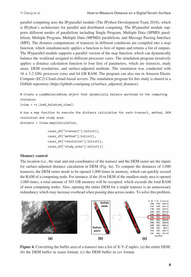
Yi Qiang et al How to Measure Distance on a Digital Terrain Surface
9
parallel computing uses the IPyparallel module (The IPython Development Team 2018) which is IPythonrsquos architecture for parallel and distributed computing The IPyparallel module sup-ports different modes of parallelism including Single Program Multiple Data (SPMD) paral-lelism Multiple Program Multiple Data (MPMD) parallelism and Message Passing Interface (MPI) The distance computations of transects in different conditions are compiled into a map function which simultaneously applies a function to lists of inputs and returns a list of outputs The IPyparallel module supports a parallel version of the map function which can dynamically balance the workload assigned to different processor cores The simulation program iteratively applies a distance calculation function to four lists of parameters which are transects study areas DEM resolutions and surface-adjusted methods The simulation was conducted with 16 times 32 GHz processor cores and 64 GB RAM The program can also run in Amazon Elastic Compute (EC2) Cloud cloud-based servers The simulation program for this study is shared in a GitHub repository (httpsgithubcomqiang -yisurfa ce_adjus ted_distance)
Create a LoadBalancedView object that dynamically balance workload to the computing
instances
lview = rcload_balanced_view()
Use a map function to execute the distance calculation for each transect method DEM
resolution and study area
distance = lviewmap(Calculation
cases_df[rsquotransectrsquo]tolist()
cases_df[rsquomethodrsquo]tolist()
cases_df[rsquoresolutionrsquo]tolist()
cases_df[rsquostudy_arearsquo]tolist())
Memory control The location (ie the start and end coordinates) of the transect and the DEM raster are the inputs for surface-adjusted distance calculation in DEM (Fig 4a) To compute the distances of 1000 transects the DEM raster needs to be opened 1000 times in memory which can quickly exceed the RAM of a computing node For instance if the 10 m DEM of the smallest study area is opened 1000 times a total amount of 503 GB memory will be occupied which exceeds the total RAM of most computing nodes Also opening the entire DEM for a single transect is an unnecessary redundancy which may increase overhead when passing data across nodes To solve this problem
Figure 4 Converting the buffer area of a transect into a list of X-Y-Z tuples (a) the entire DEM (b) the DEM buffer in raster format (c) the DEM buffer in csv format
Geographical Analysis
10
a buffer is built around each transect and only the transects and buffer areas around them are sent into a distance computation Instead of storing the buffer areas in raster which still contain nu-merous no-data pixels within the Minimum Bounding Rectangle (eg Fig 4b) pixels inside the buffer areas are converted into X-Y-Z tuples which are stored in comma-separated values (csv) files (Fig 4c) By doing so the input data size for distance calculation of a transect can be reduced from gt 100 MB to ~1 MB The data conversion process introduces additional computational cost associated with the overhead of generating csv files for each path However the smaller DEM buffers increase the efficiency of distance computation by reducing computational overhead of data transfer to and from the computing nodes and reducing overall memory requirements
Results
Distances calculated using different surface adjustment methods on DEMs of different resolu-tions are compared with the benchmark distance measured at 3 m LiDAR data using the Closest Centroid method Residuals and Root-Mean-Square Error (RMSE) metrics between the mea-sured distances and benchmark distances evaluate the measurement accuracy Processing times of distance measurement are also compared to evaluate the computational efficiency of the different interpolation methods
Residual analysisResiduals indicate discrepancies between the measured distances and benchmark distances in the simulated transects (ie measured distancemdashbenchmark distance) Fig 5 shows that the residuals of most methods (except closest centroids) are negative at finest resolutions indicat-ing underestimation but at coarser resolutions approaching zero or becoming positive As an exception the closest centroid (clos) method overestimates distances at finer resolutions and transitions to underestimation as pixel size increases Magnitude of residuals for this method is highest IN most situations except the 1000 m resolution where the residuals of the various methods converge The weighted average (wavg) residuals are generally closer to zero than all other methods while the TIN and Natural Neighbor methods have the largest negative residu-als Comparing the three polynomial methods the residuals of the bilinear method most closely approximate the benchmark (ie lowest absolute residuals) followed by the biquadratic and bicubic methods Thus the increasing complexity of the polynomial function actually reduces accuracy of distance measurement likely due to overfitting
Maximum residual values are higher for more mountainous and hilly landscapes and the mag-nitude of errors appears to relate as much or more to terrain roughness (ie elevation range as shown in Table 1) as to DEM size Washington is roughly the same size as Nebraska and yet con-tains much larger residuals Colorado is not even half the size of Louisiana and yet its residuals are larger by orders of magnitude Working across spatial resolutions the progression of residual values generated by all methods differs most strongly at 10 m and then resolves as pixel size increases to 1000 m Residuals for the three flattest terrains tend to converge at 100 m resolution diverging by 10ndash20 m as overestimation becomes evident for 1000 m pixels This finding possibly implies that variations in accuracy of the different interpolation methods relates to terrain flatness or perhaps to terrain uniformity Confirmation of this would require further characterization of the DEM surfaces
The simulated transects vary in length and the residuals are highly dependent on the tran-sect length To eliminate the effect of transect length ratios of the residuals by transect lengths were calculated to compare the measurement accuracy per distance unit Fig 6 shows that the
Yi Qiang et al How to Measure Distance on a Digital Terrain Surface
11
Fig
ure
5 M
ean
resi
dual
s (m
easu
red
in m
eter
s) b
etw
een
mea
sure
d di
stan
ces
and
benc
hmar
k di
stan
ces
at d
iffe
rent
res
olut
ions
Pos
itive
val
ues
refle
ct
over
-est
imat
ion
and
nega
tive
valu
es re
flect
und
er-e
stim
atio
n re
lativ
e to
the
LiD
AR
dat
a T
he y
-axe
s ar
e lin
ear a
nd v
ary
amon
g D
EM
s a
nd th
e x-
axes
ar
e ex
pone
ntia
l and
iden
tical
For
any
par
ticul
ar lo
catio
n an
d re
solu
tion
met
hods
with
line
s cl
oses
t to
zero
on
the
y-ax
is a
re m
ore
accu
rate
on
aver
age
Geographical Analysis
12
Fig
ure
6 M
ean
resi
dual
rat
ios
betw
een
benc
hmar
k di
stan
ces
and
mea
sure
d di
stan
ces
mea
sure
d at
dif
fere
nt r
esol
utio
ns P
ositi
ve v
alue
s re
flect
ove
r-es
timat
ion
and
nega
tive
valu
es r
eflec
t und
er-e
stim
atio
n r
elat
ive
to th
e L
iDA
R d
ata
Not
e th
at th
e y-
axes
dif
fer
acro
ss D
EM
s w
hile
the
x-ax
es a
re
cons
iste
nt a
nd lo
gari
thm
ical
ly r
esca
led
Yi Qiang et al How to Measure Distance on a Digital Terrain Surface
13
changing pattern of the ratios of residuals at different resolutions are analogous to the patterns of residuals shown in Fig 5 As shown in Fig 6 the error ratio of distance measurement for any given transect may range from minus2 to +4 depending on the surface-adjusted method the study area and on the resolution of the DEM Comparing among the study areas Louisiana has the smallest error magnitude with residual ratios ranging from ndash01 to 03 while the residual ratios in Colorado span ranging from minus02 to 27 indicating that distance measurement error tends to be larger in mountainous or uneven terrains than in flatter or smoother terrains
RMSE analysisRoot-Mean-Square Error (RMSE) indicates the absolute fit between measured distances and benchmark distances The RMSEs in Fig 7 generally confirm the patterns of residuals in Figs 5 and 6 with some interesting cross scale patterns highlighted RMSE values tend to rise as pixel size increases from 100 m with RMSE increasing for North Carolina and Colorado for 30 m and larger pixels Method-specific errors show greatest differences at finer resolutions resolv-ing to a value ranging between roughly 450 m (Nebraska) and 600 m (all other study areas) at 1000 m resolution The range of average error among methods is higher for mountainous and hilly landscapes with almost no difference among methods for the two flattest landscapes (Texas and Louisiana) The Weighted Average method generates the lowest RMSE magnitudes overall although the Closest Centroid method gives lower RMSE values at 100 m resolution for reasons that are not clear The bilinear method has the lowest RMSE of all three polynomial methods followed by the biquadratic and bicubic method
Processing timeProcessing time of the distance calculation increases at finer resolutions (ie as cell size de-creases) (Fig 8) TIN and Nearest Neighbor require the longest processing times except for North Carolina at 10 m resolution Shortest processing times are used by Weighted Average and Closest Centroid followed by the bilinear polynomial Processing times drop considerably for coarser resolution DEMs because of relatively fewer pixels Considering the changing patterns of residuals and RMSEs however there is a trade-off between accuracy and computational efficiency
Comparing among the different methods the Natural Neighbor and TIN method require the longest processing time in most landscapes Given their high residuals and RMSEs these two methods seem the least optimal for surface-adjusted distance calculation And while the Closest Centroid method takes the shortest processing time the accuracy metrics indicate that its utility for surface-adjusted distance estimation is highly varied and thus not consistently reliable The bilinear polynomial method gives more accurate estimations but takes additional processing time especially at fine resolutions Given the low absolute residuals and RMSEs in most landscapes and at most resolutions the weighted average method can be considered the sur-face adjusting method that best balances accuracy with processing time for distance calculation
Discussion and implications
This study applies a HPC-enabled Monte-Carlo simulation to evaluate seven surface adjustment methods for distance calculation on digital terrain Distances of 1000 randomly generated tran-sects were calculated in six study areas using different surface adjusting methods and DEMs at different resolutions The calculated distances were compared with benchmark distances
Geographical Analysis
14
Fig
ure
7 R
MSE
(m
easu
red
in m
eter
s) b
etw
een
benc
hmar
k di
stan
ces
and
mea
sure
d di
stan
ces
mea
sure
d in
dif
fere
nt r
esol
utio
ns N
ote
that
the
y-ax
es
are
scal
ed d
iffe
rent
ly a
cros
s pa
nels
Yi Qiang et al How to Measure Distance on a Digital Terrain Surface
15
Fig
ure
8 M
ean
proc
essi
ng ti
mes
(mea
sure
d in
sec
onds
) for
sur
face
-adj
uste
d di
stan
ce c
alcu
latio
n pe
r tra
nsec
t usi
ng d
iffe
rent
met
hods
and
at d
iffe
rent
re
solu
tions
Not
e th
at y
-axi
s va
lues
dif
fer
amon
g D
EM
s w
hile
x-a
xis
valu
es a
re id
entic
al
Geographical Analysis
16
measured on 3 m resolution DEMs to evaluate their accuracies Residuals and RMSEs compared measured distances with LiDAR benchmark distances To reduce the overall computing time the distance calculation algorithm was optimized to reduce memory usage and processing time in a multi-core computer
The major findings in this study include (1) the distance measurement varies with DEM res-olutions surface adjustment methods and terrain types (2) Weighted Average is overall the most accurate surface adjustment for distance measurement with a few exceptions (3) there is a trade-off between DEM resolution and computing time The assessment results provide a foundation for distance-based spatial analyses on terrain surface (eg distance-based point pattern analysis and kriging interpolation) In a broader sense the study increases the understanding about the interplay between analytic methods scale and the geographical phenomena being studied
The assessment reveals the dependency of distance measurement on data resolution surface adjustment methods and terrain variations The results show a pattern of distance underestimation relative to the LiDAR benchmarks at finer resolutions (10 m and 30 m) that transitions to near equivalence or slight overestimation as pixel size increases The degree of underestimation varies with method of surface adjustment The weighted average method has the highest accuracy overall in most situations This finding may seem surprising given that the method utilizes a search neigh-borhood of only 8 adjacent pixels In terrain with high local relief one might expect that the polyno-mial methods would provide better results due to larger neighborhoods andor adjustment methods that could filter localized perturbations in elevation The results indicate that biquadratic (8 neigh-bors) and the bicubic (16 neighbors) methods tend to exaggerate underestimation While the bilinear neighborhood (4 pixels) produces residuals and RMSE values closer to the weighted average the kernel is rarely centered on the point being adjusted and this can over- or underemphasize nearby terrain nonuniformity Closest Centroid TIN and Nearest Neighbor employ even smaller neighbor-hoods (1 3 and up to 6 neighbors respectively) further exacerbating the problem Overestimation of surface-adjusted distance for all methods at 1000 m resolution may be associated with neigh-borhood bias as well the spatial extent of larger pixels may ignore local features at the same time as weighting more distant features (up to 4 8 or 16 kilometers away) in equal consideration The weighted average method adjustment is based on central tendency and qualified by inverse distance weighting which can offset the impacts of rough or uneven terrain in more distant pixels
The balance between improved accuracy and extra processing time is relevant from a prac-tical standpoint The DEMs tested here are probably too small to be useful for regional or conti-nental modeling as for example studies involving sea level rise earthquake damage or coastal storm events Even with high performance computing distance adjustment for larger study areas could require minutes or longer Moreover distance estimation is often the initial step and rarely the final product of spatial modeling The Closest Centroid method calculates distance based on elevation in rigid pixels which does not adjust the terrain surface using surrounding elevation values Thus the distance measurements of this method fluctuate at different resolutions due to the stair-step effect of DEM pixels As a consequence the method tends to over-estimate distance at finer resolutions due to including too many (small) pixels and to under-estimate distance at coarser resolutions due to averaging within large pixels Despite carrying the lowest processing time the accuracy of the Closest Centroid method should not be considered a good choice when trying to balance accuracy with processing times Higher processing times shown by TIN and Nearest Neighbor are coupled with reduced accuracy and no balance is achieved Polynomial adjustment by second and third order equations reflects similar results Given the second lowest processing time the weighted average method can be considered the optimal surface adjusting
Yi Qiang et al How to Measure Distance on a Digital Terrain Surface
17
method for distance calculation in most situations Adjustment using bilinear polynomial estima-tion can be considered an alternative with slightly less improvement in accuracy
The accuracy of the surface adjustment methods also varies in different terrain types The ac-curacy difference among methods is smallest in flat terrain such as Louisiana and Texas implying that for these terrain types the choice of surface adjustment for distance measurements matters less than for hilly and mountainous terrain Differences in error metrics for more mountainous or nonuniform terrains show greater variation especially at fine and intermediate resolutions mean-ing the choice of surface adjustment appears to have a greater impact on distance estimation in rougher terrain and at finer resolutions Error magnitudes begin to coalesce after 100 m resolution for all methods indicating that at some point the extra computations required for surface adjust-ment are simply not worth the potential improvement in accuracy Accuracy of surface-adjusted distance measurement is reduced in DEMs that contain a mix of terrain types with some flat and some hilly areas Future research must investigate the relationships between terrain roughness terrain uniformity and accuracy to better understand the full implication of these findings
As an additional note methods that perform best for distance calculation may or may not be optimal for other tasks such as estimating surface-adjusted elevation or area Ghandehari Buttenfield and Farmer (2019) demonstrate that linear and bilinear polynomials give slightly better accuracies for surface-adjusted estimation of point elevation on DEMs although errors for any method are quite small on the order of centimeter magnitudes for terrain measured in me-ters Their study shows however that errors for all methods increase in rough terrain This reflects earlier research by Shi and Tian (2006) and Schneider (2001) showing that errors in elevation estimation are more prominent in rough terrain Ghandehari and Buttenfield (2018) compare sur-face-adjusted methods for estimating pixel surface areas finding that while a bicubic polynomial estimation gives the highest accuracy relative to a 3 m LiDAR benchmark it carries unreason-ably high processing times They modify Jennessrsquo (2004) surface area estimation method and then apply bilinear polynomial estimation to achieve nearly equivalent accuracies to the bicubic method with processing times reduced by nearly 80 (Ghandehari 2019)
As the primary objective of the study is to evaluate and compare among surface adjustment methods the simulation program is implemented in a simple parallel model which effectively reduces the computing time to a manageable level The performance of the simulation can be further improved with finer grain parallelism architectures such as OpenMP and MPI Also the program can be further parallelized by including on-the-fly transect generation and buffer area extraction These optimization options will be explored in future experiments such as surface-ad-justed area calculation for a new variety of case studies
The title of this article raises the issue of why accurate distance measurements matters in geographical analysis There are several reasons First and as described at the beginning of the article distance metrics underlie many if not most simple and compound GIS analytic methods Second it stands to reason that inaccurate distances can propagate inaccuracies throughout the entire course of spatial modeling and confound any estimates related to terrain surfaces as for ex-ample glacial recession wetlands fragmentation freight routing or debris flow estimation Third digital terrain is one of the most frequently included data layers in spatial analyses Bolstad (2019 p 485) cites the influence of terrain characteristics on a broad set of environmental functions such as soil moisture agricultural yields sediment transport and construction costs Wilson (2012 p 107) explains the important impact of terrain ldquohellip in modulating the atmospheric geomor-phic hydrologic and ecological processes operating on or near the Earthrsquos surfacerdquo He refers to Hutchinson and Gallant (2000) in arguing that the terrain is so tightly coupled with these four
Geographical Analysis
18
families of processes that characterization of the terrain directly leads to and refines insights about the nature of the processes In a nutshell geospatial analytics cannot be accurate without accurate distance metrics And because most geographic and geomorphic processes depend partially or wholly upon the land surface on which they are situated distance measurements should be per-formed on the terrain surface ldquoas the horse runsrdquo instead of ldquoas the crow fliesrdquo
With the emergence of parallel processing and the increased availability of fine resolution terrain data surface-adjusted distance metrics are becoming an operational strategy that can improve the accuracy of many types of spatial modeling although results depend upon several factors (resolution terrain type and uniformity and surface adjustment method) Three of those factors have been examined here but this study has limitations that call for additional examina-tion and assessment The characterization of terrain uniformity must be examined more formally along with possible interaction among the factors analyzed in this article Additionally the opti-mal methods choices need to be further tested and validated by embedding the surface-adjusted distance metrics into more complex analytics For instance a hypothesis to be tested is whether surface-adjusted distance can increase the accuracy of kriging interpolation Surface adjustment also needs to be embedded in full-blown surface process models to understand them in analytic practice And finally the assessment of distance measurement shows that choosing an appropri-ate (not necessarily the finest) scale is important for spatial analysis and modeling Quattrochi and Goodchild (1997) suggest that geographical analyses should be conducted at the operational scale (also referred to by Montello (2001) as phenomenon scale) where the studied processes operate since slight changes in these processes can invoke pronounced changes in model results The results reported in this study reveal that the optimal DEM resolutions for distance mea-surement varies among different surface adjustment methods and terrain types Importantly the choice of a method may also depend upon task (measuring distance surface area or volume) As distance is the most fundamental metric for geographical analyses the knowledge generated in this study lays a foundation for developing scale-sensitive analysis tools on a terrain surface
Acknowledgment
The authors acknowledge excellent and constructive comments from reviewers which strength-ened the text
Funding information
This article is based on work supported by the US National Science under the Methodology Measurement amp Stats (MMS) Program (Award No 1853866) This article is also based on work that is part of the Data Harmonization Initiative at Earth Lab (httpswwwcolor adoeduearth lab) supported by an investment from the University of Colorado Grand Challenge Initiative Any opinions findings and conclusions or recommendations expressed in this material are those of the authors and do not necessarily reflect the views of the funding agencies
Appendix
This appendix documents the data sets and their download sources used for the experiments in the manuscript The exact specifications are included here in the interests of reproducible sci-ence so that interested readers can replicate the study using the same data sets
Yi Qiang et al How to Measure Distance on a Digital Terrain Surface
19
Benchmark LiDAR data
State Benchmark LiDAR datasets
Colorado 2010 South San Luis Lakes LidarNebraska 2009 Nebraska Department of Natural Resources (DNR) South Central
Nebraska LidarNorth Carolina 2003 North Carolina Floodplain Mapping Program (NCFMP) LidarTexas 2011 Texas Natural Resources Information System (TNRIS) Lidar Bell
Burnet and McLennan CountiesWashington 2006 USGS Lidar North Puget Sound WashingtonLouisiana 1999 Louisiana Lidar Project (1999ndash2008)
Tiles of 10 m DEMsThe following tiles are available to download in USGS TNM Download httpsviewernatio nalmapgovbasic
State Tiles of 10 m DEM
Colorado USGS NED ned19_n39x25_w106x25_co_arkansasvalley_2010 19 arc-second 2012 15 times 15 min IMGUSGS NED ned19_n39x00_w106x50_co_arkansasvalley_2010 19 arc-second 2012 15 times 15 min IMGUSGS NED ned19_n38x75_w106x00_co_arkansasvalley_2010 19 arc-second 2012 15 times 15 min IMGUSGS NED ned19_n39x50_w106x00_co_grandco_2010 19 arc-second 2011 15 times 15 min IMGUSGS NED ned19_n38x75_w106x50_co_arkansasvalley_2010 19 arc-second 2012 15 times 15 min IMGUSGS NED ned19_n38x25_w106x25_co_sanluisvalley_2011 19 arc-second 2012 15 times 15 min IMGUSGS NED ned19_n38x50_w106x00_co_arkansasvalley_2010 19 arc-second 2012 15 times 15 min IMGUSGS NED ned19_n38x25_w106x00_co_arkansasvalley_2010 19 arc-second 2012 15 times 15 min IMGUSGS NED ned19_n38x25_w106x25_co_arkansasvalley_2 010 19 arc-second 2012 15 times 15 min IMGUSGS NED ned19_n39x25_w106x50_co_arkansasvalley_2010 19 arc-second 2012 15 times 15 min IMGUSGS NED ned19_n38x25_w106x00_co_sanluisvalley_2011 19 arc-second 2012 15 times 15 min IMGUSGS NED ned19_n39x00_w106x00_co_arkansasvalley_2010 19 arc-second 2012 15 times 15 min IMGUSGS NED ned19_n39x50_w106x25_co_arkansasvalley_2010 19 arc-second 2012 15 times 15 min IMGUSGS NED ned19_n38x50_w106x25_co_arkansasvalley_2010 19 arc-second 2012 15 times 15 min IMGUSGS NED ned19_n38x25_w106x50_co_sanluisvalley_2011 19 arc-second 2012 15 times 15 min IMG
Geographical Analysis
20
State Tiles of 10 m DEM
USGS NED ned19_n39x50_w106x50_co_arkansasvalley_2010 19 arc-second 2012 15 times 15 min IMGUSGS NED ned19_n38x75_w106x25_co_arkansasvalley_2010 19 arc-second 2012 15 times 15 min IMGUSGS NED ned19_n39x00_w106x25_co_arkansasvalley_2010 19 arc-second 2012 15 times 15 min IMGUSGS NED ned19_n38x25_w105x75_co_sanluisvalley_2011 19 arc-second 2012 15 times 15 min IMGUSGS NED ned19_n39x75_w106x00_co_grandco_2010 19 arc-second 2011 15 times 15 min IMGUSGS NED ned19_n38x00_w106x25_co_sanluisvalley_2011 19 arc-second 2012 15 times 15 min IMGUSGS NED ned19_n38x00_w106x00_co_sanluisvalley_2011 19 arc-second 2012 15 times 15 min IMGUSGS NED ned19_n38x00_w106x50_co_sanluisvalley_2011 19 arc-second 2012 15 times 15 min IMGUSGS NED ned19_n38x00_w105x75_co_sanluisvalley_2011 19 arc-second 2012 15 times 15 min IMG
Nebraska USGS NED ned19_n40x50_w100x25_ne_rainwater_2009 19 arc-second 2011 15 times 15 min IMGUSGS NED ned19_n40x50_w100x00_ne_rainwater_2009 19 arc-second 2011 15 times 15 min IMGUSGS NED ned19_n40x50_w100x50_ne_rainwater_2009 19 arc-second 2011 15 times 15 min IMGUSGS NED ned19_n40x75_w100x75_ne_rainwater_2009 19 arc-second 2011 15 times 15 min IMGUSGS NED ned19_n40x75_w100x00_ne_rainwater_2009 19 arc-second 2011 15 times 15 min IMGUSGS NED ned19_n40x75_w100x25_ne_rainwater_2009 19 arc-second 2011 15 times 15 min IMGUSGS NED ned19_n40x75_w100x50_ne_rainwater_2009 19 arc-second 2011 15 times 15 min IMGUSGS NED ned19_n40x50_w100x75_ne_rainwater_2009 19 arc-second 2011 15 times 15 min IMGUSGS NED ned19_n40x75_w101x00_ne_rainwater_2009 19 arc-second 2011 15 times 15 min IMGUSGS NED ned19_n40x50_w101x00_ne_rainwater_2009 19 arc-second 2011 15 times 15 min IMGUSGS NED ned19_n40x25_w100x00_ne_rainwater_2009 19 arc-second 2011 15 times 15 min IMGUSGS NED ned19_n40x25_w100x50_ne_rainwater_2009 19 arc-second 2011 15 times 15 min IMGUSGS NED ned19_n40x25_w100x25_ne_rainwater_2009 19 arc-second 2011 15 times 15 min IMG
Yi Qiang et al How to Measure Distance on a Digital Terrain Surface
21
State Tiles of 10 m DEM
USGS NED ned19_n40x25_w100x75_ne_rainwater_2009 19 arc-second 2011 15 times 15 min IMGUSGS NED ned19_n41x00_w100x75_ne_rainwater_2009 19 arc-second 2011 15 times 15 min IMGUSGS NED ned19_n41x00_w100x00_ne_rainwater_2009 19 arc-second 2011 15 times 15 min IMGUSGS NED ned19_n41x00_w100x50_ne_rainwater_2009 19 arc-second 2011 15 times 15 min IMGUSGS NED ned19_n41x00_w100x25_ne_rainwater_2009 19 arc-second 2011 15 times 15 min IMGUSGS NED ned19_n40x75_w099x75_ne_rainwater_2009 19 arc-second 2011 15 times 15 min IMGUSGS NED ned19_n40x50_w099x75_ne_rainwater_2009 19 arc-second 2011 15 times 15 min IMGUSGS NED ned19_n40x25_w101x00_ne_rainwater_2009 19 arc-second 2011 15 times 15 min IMGUSGS NED ned19_n41x00_w101x00_ne_rainwater_2009 19 arc-second 2011 15 times 15 min IMGUSGS NED ned19_n40x25_w099x75_ne_rainwater_2009 19 arc-second 2011 15 times 15 min IMGUSGS NED ned19_n41x00_w099x75_ne_rainwater_2009 19 arc-second 2011 15 times 15 min IMG
North Carolina
USGS NED ned19_n36x00_w081x50_nc_statewide_2003 19 arc-second 2012 15 times 15 min IMGUSGS NED ned19_n36x00_w082x00_nc_statewide_2003 19 arc-second 2012 15 times 15 min IMGUSGS NED ned19_n36x00_w081x25_nc_statewide_2003 19 arc-second 2012 15 times 15 min IMGUSGS NED ned19_n36x00_w081x75_nc_statewide_2003 19 arc-second 2012 15 times 15 min IMGUSGS NED ned19_n36x00_w081x00_nc_statewide_2003 19 arc-second 2012 15 times 15 min IMGUSGS NED ned19_n36x00_w082x25_nc_statewide_2003 19 arc-second 2012 15 times 15 min IMGUSGS NED ned19_n35x75_w082x00_nc_statewide_2003 19 arc-second 2012 15 times 15 min IMGUSGS NED ned19_n35x75_w081x25_nc_statewide_2003 19 arc-second 2012 15 times 15 min IMGUSGS NED ned19_n35x75_w081x50_nc_statewide_2003 19 arc-second 2012 15 times 15 min IMGUSGS NED ned19_n35x75_w081x75_nc_statewide_2003 19 arc-second 2012 15 times 15 min IMGUSGS NED ned19_n35x75_w081x00_nc_statewide_2003 19 arc-second 2012 15 times 15 min IMG
Geographical Analysis
22
State Tiles of 10 m DEM
USGS NED ned19_n35x75_w082x25_nc_statewide_2003 19 arc-second 2012 15 times 15 min IMGUSGS NED ned19_n36x25_w081x50_nc_statewide_2003 19 arc-second 2012 15 times 15 min IMGUSGS NED ned19_n36x25_w081x00_nc_statewide_2003 19 arc-second 2012 15 times 15 min IMGUSGS NED ned19_n36x25_w081x25_nc_statewide_2003 19 arc-second 2012 15 times 15 min IMGUSGS NED ned19_n36x25_w082x00_nc_statewide_2003 19 arc-second 2012 15 times 15 min IMGUSGS NED ned19_n36x25_w081x75_nc_statewide_2003 19 arc-second 2012 15 times 15 min IMGUSGS NED ned19_n36x25_w082x25_nc_statewide_2003 19 arc-second 2012 15 times 15 min IMGUSGS NED ned19_n36x00_w080x75_nc_statewide_2003 19 arc-second 2012 15 times 15 min IMGUSGS NED ned19_n35x75_w080x75_nc_statewide_2003 19 arc-second 2012 15 times 15 min IMGUSGS NED ned19_n36x25_w080x75_nc_statewide_2003 19 arc-second 2012 15 times 15 min IMG
Texas USGS NED ned19_n31x50_w097x50_tx_bellburnetmclennancos_2011 19 arc-second 2012 15 times 15 min IMGUSGS NED ned19_n31x25_w097x25_tx_bellburnetmclennancos_2011 19 arc-second 2012 15 times 15 min IMGUSGS NED ned19_n31x00_w098x25_tx_bellburnetmclennancos_2011 19 arc-second 2012 15 times 15 min IMGUSGS NED ned19_n31x25_w097x50_tx_bellburnetmclennancos_2011 19 arc-second 2012 15 times 15 min IMGUSGS NED ned19_n31x50_w097x75_tx_bellburnetmclennancos_2011 19 arc-second 2012 15 times 15 min IMGUSGS NED ned19_n31x75_w097x25_tx_bellburnetmclennancos_2011 19 arc-second 2012 15 times 15 min IMGUSGS NED ned19_n31x25_w098x25_tx_bellburnetmclennancos_2011 19 arc-second 2012 15 times 15 min IMGUSGS NED ned19_n31x00_w098x00_tx_bellburnetmclennancos_2011 19 arc-second 2012 15 timestimes 15 min IMGUSGS NED ned19_n31x25_w097x75_tx_bellburnetmclennancos_2011 19 arc-second 2012 15 times 15 min IMGUSGS NED ned19_n31x00_w097x50_tx_bellburnetmclennancos_2011 19 arc-second 2012 15 times 15 min IMGUSGS NED ned19_n31x00_w097x75_tx_bellburnetmclennancos_2011 19 arc-second 2012 15 times 15 min IMGUSGS NED ned19_n31x75_w097x50_tx_bellburnetmclennancos_2011 19 arc-second 2012 15 times 15 min IMG
Yi Qiang et al How to Measure Distance on a Digital Terrain Surface
23
State Tiles of 10 m DEM
USGS NED ned19_n31x25_w098x00_tx_bellburnetmclennancos_2011 19 arc-second 2012 15 times 15 min IMGUSGS NED ned19_n31x00_w097x25_tx_bellburnetmclennancos_2011 19 arc-second 2012 15 times 15 min IMGUSGS NED ned19_n31x50_w097x25_tx_bellburnetmclennancos_2011 19 arc-second 2012 15 times 15 min IMGUSGS NED ned19_n30x75_w098x25_tx_bellburnetmclennancos_2011 19 arc-second 2012 15 times 15 min IMGUSGS NED ned19_n30x75_w098x00_tx_bellburnetmclennancos_2011 19 arc-second 2012 15 times 15 min IMGUSGS NED ned19_n30x75_w097x50_tx_bellburnetmclennancos_2011 19 arc-second 2012 15 times 15 min IMGUSGS NED ned19_n30x75_w098x00_tx_central_llano_2007 19 arc-second 2010 15 times 15 min IMGUSGS NED ned19_n30x75_w098x25_tx_central_llano_2007 19 arc-second 2010 15 times 15 min IMGUSGS NED ned19_n31x75_w097x00_tx_bellburnetmclennancos_2011 19 arc-second 2012 15 times 15 min IMGUSGS NED ned19_n31x50_w097x00_tx_bellburnetmclennancos_2011 19 arc-second 2012 15 times 15 min IMGUSGS NED ned19_n31x25_w098x50_tx_central_llano_2007 19 arc-second 2010 15 times 15 min IMGUSGS NED ned19_n31x50_w098x50_tx_central_llano_2007 19 arc-second 2010 15 times 15 min IMGUSGS NED ned19_n31x00_w098x50_tx_central_llano_2007 19 arc-second 2010 15 times 15 min IMGUSGS NED ned19_n31x75_w098x50_tx_central_llano_2007 19 arc-second 2010 15 times 15 min IMGUSGS NED ned19_n31x00_w098x50_tx_bellburnetmclennancos_2011 19 arc-second 2012 15 times 15 min IMGUSGS NED ned19_n30x75_w098x50_tx_central_llano_2007 19 arc-second 2010 15 times 15 min IMGUSGS NED ned19_n30x75_w098x50_tx_bellburnetmclennancos_2011 19 arc-second 2012 15 times 15 min IMG
Washington USGS NED ned19_n48x50_w122x00_wa_northpugetsound_2006 19 arc-second 2009 15 times 15 min IMGUSGS NED ned19_n48x50_w122x50_wa_puget_sound_2000 19 arc-second 2012 15 times 15 min IMGUSGS NED ned19_n48x50_w121x50_wa_northpugetsound_2006 19 arc-second 2009 15 times 15 min IMGUSGS NED ned19_n49x00_w122x50_wa_northpugetsound_2006 19 arc-second 2009 15 times 15 min IMGUSGS NED ned19_n48x75_w122x75_wa_sanjuanco_2009 19 arc-second 2011 15 times 15 min IMG
Geographical Analysis
24
State Tiles of 10 m DEM
USGS NED ned19_n48x50_w122x25_wa_northpugetsound_2006 19 arc-second 2009 15 times 15 min IMGUSGS NED ned19_n48x75_w121x25_wa_northpugetsound_2006 19 arc-second 2009 15 times 15 min IMGUSGS NED ned19_n49x00_w121x25_wa_northpugetsound_2006 19 arc-second 2009 15 times 15 min IMGUSGS NED ned19_n49x00_w122x00_wa_northpugetsound_2006 19 arc-second 2009 15 times 15 min IMGUSGS NED ned19_n48x50_w122x75_wa_puget_sound_2000 19 arc-second 2012 15 times 15 min IMGUSGS NED ned19_n48x75_w122x00_wa_northpugetsound_2006 19 arc-second 2009 15 times 15 min IMGUSGS NED ned19_n48x75_w122x75_wa_northpugetsound_2006 19 arc-second 2009 15 times 15 min IMGUSGS NED ned19_n48x75_w121x75_wa_northpugetsound_2006 19 arc-second 2009 15 times 15 min IMGUSGS NED ned19_n48x75_w122x25_wa_northpugetsound_2006 19 arc-second 2009 15 times 15 min IMGUSGS NED ned19_n49x00_w121x75_wa_northpugetsound_2006 19 arc-second 2009 15 times 15 min IMGUSGS NED ned19_n48x75_w122x50_wa_northpugetsound_2006 19 arc-second 2009 15 times 15 min IMGUSGS NED ned19_n49x00_w122x25_wa_northpugetsound_2006 19 arc-second 2009 15 times 15 min IMGUSGS NED ned19_n48x50_w122x50_wa_northpugetsound_2006 19 arc-second 2009 15 times 15 min IMGUSGS NED ned19_n48x50_w122x75_wa_northpugetsound_2006 19 arc-second 2009 15 times 15 min IMGUSGS NED ned19_n48x75_w121x50_wa_northpugetsound_2006 19 arc-second 2009 15 times 15 min IMGUSGS NED ned19_n49x00_w122x75_wa_northpugetsound_2006 19 arc-second 2009 15 times 15 min IMGUSGS NED ned19_n48x50_w121x75_wa_northpugetsound_2006 19 arc-second 2009 15 times 15 min IMGUSGS NED ned19_n49x25_w122x25_wa_northpugetsound_2006 19 arc-second 2009 15 times 15 min IMGUSGS NED ned19_n49x25_w122x50_wa_northpugetsound_2006 19 arc-second 2009 15 times 15 min IMGUSGS NED ned19_n49x25_w122x00_wa_northpugetsound_2006 19 arc-second 2009 15 times 15 min IMGUSGS NED ned19_n49x25_w122x75_wa_northpugetsound_2006 19 arc-second 2009 15 times 15 min IMGUSGS NED ned19_n48x25_w122x50_wa_puget_sound_2000 19 arc-second 2012 15 times 15 min IMG
Yi Qiang et al How to Measure Distance on a Digital Terrain Surface
25
State Tiles of 10 m DEM
USGS NED ned19_n48x25_w122x75_wa_puget_sound_2000 19 arc-second 2012 15 times 15 min IMGUSGS NED ned19_n48x50_w123x00_wa_puget_sound_2000 19 arc-second 2012 15 times 15 min IMGUSGS NED ned19_n48x75_w123x00_wa_sanjuanco_2009 19 arc-second 2011 15 times 15 min IMGUSGS NED ned19_n49x00_w123x00_wa_northpugetsound_2006 19 arc-second 2009 15 times 15 min IMGUSGS NED ned19_n48x50_w123x00_wa_sanjuanco_2009 19 arc-second 2011 15 times 15 min IMGUSGS NED ned19_n49x25_w123x00_wa_northpugetsound_2006 19 arc-second 2009 15 times 15 min IMGUSGS NED ned19_n48x25_w123x00_wa_puget_sound_2000 19 arc-second 2012 15 times 15 min IMG
Louisiana USGS NED ned19_n30x75_w091x50_la_statewide_2006 19 arc-second 2009 15 times 15 min IMGUSGS NED ned19_n30x50_w091x00_la_statewide_2006 19 arc-second 2009 15 times 15 min IMGUSGS NED ned19_n30x50_w091x50_la_atchafalayabasin_2010 19 arc-second 2011 15 times 15 min IMGUSGS NED ned19_n30x50_w091x50_la_statewide_2006 19 arc-second 2009 15 times 15 min IMGUSGS NED ned19_n30x75_w091x00_la_statewide_2006 19 arc-second 2009 15 times 15 min IMGUSGS NED ned19_n30x75_w091x25_la_statewide_2006 19 arc-second 2009 15 times 15 min IMGUSGS NED ned19_n30x75_w090x75_la_statewide_2006 19 arc-second 2009 15 times 15 min IMGUSGS NED ned19_n30x50_w091x25_la_statewide_2006 19 arc-second 2009 15 times 15 min IMGUSGS NED ned19_n30x50_w090x75_la_statewide_2006 19 arc-second 2009 15 times 15 min IMGUSGS NED ned19_n30x50_w091x50_LA-USGS_Atchafalaya2_2012_2014 19 arc-second 20140615 15 15 min IMGUSGS NED ned19_n31x00_w091x50_la_statewide_2006 19 arc-second 2009 15 times 15 min IMGUSGS NED ned19_n31x00_w091x25_la_statewide_2006 19 arc-second 2009 15 times 15 min IMGUSGS NED ned19_n31x00_w091x00_la_statewide_2006 19 arc-second 2009 15 times 15 min IMGUSGS NED ned19_n31x00_w090x75_la_statewide_2006 19 arc-second 2009 15 times 15 min IMGUSGS NED ned19_n30x25_w091x00_la_statewide_2006 19 arc-second 2009 15 times 15 min IMG
Geographical Analysis
26
State Tiles of 10 m DEM
USGS NED ned19_n30x25_w091x50_la_atchafalayabasin_2010 19 arc-second 2011 15 times 15 min IMGUSGS NED ned19_n30x25_w091x50_la_statewide_2006 19 arc-second 2009 15 times 15 min IMGUSGS NED ned19_n30x25_w090x75_la_statewide_2006 19 arc-second 2009 15 times 15 min IMGUSGS NED ned19_n30x25_w091x25_la_statewide_2006 19 arc-second 2009 15 times 15 min IMGUSGS NED ned19_n30x25_w091x50_LA-USGS_Atchafalaya2_2012_2014 19 arc-second 20140615 15 times 15 min IMGUSGS NED ned19_n30x25_w091x25_LA-USGS_Atchafalaya2_2012_2014 19 arc-second 20140615 15 times 15 min IMGUSGS NED ned19_n30x75_w090x50_la_statewide_2006 19 arc-second 2009 15 times 15 min IMGUSGS NED ned19_n30x50_w090x50_la_statewide_2006 19 arc-second 2009 15 times 15 min IMGUSGS NED ned19_n30x75_w091x75_la_statewide_2006 19 arc-second 2009 15 times 15 min IMGUSGS NED ned19_n30x50_w091x75_la_atchafalayabasin_2010 19 arc-second 2011 15 times 15 min IMGUSGS NED ned19_n30x50_w091x75_la_statewide_2006 19 arc-second 2009 15 times 15 min IMGUSGS NED ned19_n30x75_w091x75_la_atchafalayabasin_2010 19 arc-second 2011 15 times 15 min IMGUSGS NED ned19_n30x75_w091x75_LA-USGS_Atchafalaya2_2012_2014 19 arc-second 20140615 15 times 15 min IMGUSGS NED ned19_n30x50_w091x75_LA-USGS_Atchafalaya2_2012_2014 19 arc-second 20140615 15 times 15 min IMGUSGS NED ned19_n31x00_w090x50_la_statewide_2006 19 arc-second 2009 15 times 15 min IMGUSGS NED ned19_n30x25_w090x50_la_statewide_2006 19 arc-second 2009 15 times 15 min IMGUSGS NED ned19_n31x00_w091x75_la_statewide_2006 19 arc-second 2009 15 times 15 min IMGUSGS NED ned19_n31x00_w091x75_LA-USGS_Atchafalaya2_2012_2014 19 arc-second 20140615 15 times 15 min IMGUSGS NED ned19_n30x25_w091x75_la_atchafalayabasin_2010 19 arc-second 2011 15 times 15 min IMGUSGS NED ned19_n30x25_w091x75_la_statewide_2006 19 arc-second 2009 15 times 15 min IMGUSGS NED ned19_n30x25_w091x75_LA-USGS_Atchafalaya2_2012_2014 19 arc-second 20140615 15 times 15 min IMG
Tiles of 30 m DEMs
Yi Qiang et al How to Measure Distance on a Digital Terrain Surface
27
The following tiles are available to download in USGS TNM Download httpsviewernatio nalmapgovbasic
State Tiles of 30 m DEM
Colorado USGS NED 13 arc-second n40w107USGS NED n39w107 13 arc-secondUSGS NED 13 arc-second n40w106USGS NED 13 arc-second n39w106
Nebraska USGS NED 13 arc-second n41w101 1 x 1 degree ArcGrid 2019USGS NED 13 arc-second n41w100 1 x 1 degree ArcGrid 2019
North Carolina USGS NED 13 arc-second n36w082 1 x 1 degree ArcGrid 2019USGS NED n36w081 13 arc-second 2013 1 x 1 degree ArcGridUSGS NED 13 arc-second n36w083 1 x 1 degree ArcGrid 2017USGS NED 13 arc-second n37w082 1 x 1 degree ArcGrid 2019USGS NED 13 arc-second n37w081 1 x 1 degree ArcGrid 2018USGS NED 13 arc-second n37w083 1 x 1 degree ArcGrid 2018
Texas USGS NED 13 arc-second n32w098 1 x 1 degree ArcGrid 2019USGS NED 13 arc-second n31w098 1 x 1 degree ArcGrid 2019USGS NED 13 arc-second n32w099 1 x 1 degree ArcGrid 2019USGS NED 13 arc-second n31w099 1 x 1 degree ArcGrid 2019USGS NED 13 arc-second n32w097 1 x 1 degree ArcGrid 2019USGS NED 13 arc-second n31w097 1 x 1 degree ArcGrid 2019
Washington USGS NED 13 arc-second n49w122 1 x 1 degree ArcGrid 2018USGS NED 13 arc-second n49w123 1 x 1 degree ArcGrid 2019USGS NED 13 arc-second n50w122 1 x 1 degree ArcGrid 2018USGS NED 13 arc-second n49w121 1 x 1 degree ArcGrid 2018USGS NED 13 arc-second n50w123 1 x 1 degree ArcGrid 2018
Louisiana USGS NED 13 arc-second n31w091 1 x 1 degree ArcGrid 2019USGS NED 13 arc-second n31w092 1 x 1 degree ArcGrid 2019
Tiles of 100 m and 1000 m DEMsThe following tiles are available to download in USGSrsquos website httpsddscrusgsgovsrtmversi on2_1
States Tiles 100 m DEM Tiles 1000 m DEM
Colorado N38W107SRTMGL3 w140n40SRTM30N39W107SRTMGL3N39W106SRTMGL3N38W106SRTMGL3
Nebraska N40W100SRTMGL3 w140n90SRTM30N40W101SRTMGL3
North Carolina N35W082SRTMGL3 w140n90SRTM30N35W081SRTMGL3N35W083SRTMGL3
Texas N29W098SRTMGL3N29W099SRTMGL3
Washington N48W123SRTMGL3 w100n40SRTM30N48W122SRTMGL3
Louisiana N29W091SRTMGL3 w100n40SRTM30N29W092SRTMGL3
Geographical Analysis
28
Tab
les
of
the
anal
ysis
res
ult
s
Tab
le A
1 R
esid
ual
Ave
rage
Res
idua
l R
MSE
and
Pro
cess
ing
Tim
e fo
r W
ashi
ngto
n I
nter
pola
tion
Met
hods
Inc
lude
(in
Top
-to-
Bot
tom
Ord
er)
Bic
ubic
Bili
near
and
Biq
uadr
atic
pol
ynom
ials
Clo
sest
Cen
troi
d N
eare
st N
eigh
bor
Tri
angu
late
d Ir
regu
lar
Net
wor
k a
nd W
eigh
ted
Ave
rage
Res
olut
ion
Stud
y ar
eaIn
terp
olat
ion
met
hod
Avg
res
idua
l (m
)A
vg t
ime
(s)
Avg
rat
io o
f re
sidu
alR
MSE
(m
)
10W
ashi
ngto
nbi
Cub
minus474
29
231
60minus0
016
0859
825
10W
ashi
ngto
nbi
Lin
minus275
87
210
59minus0
009
4235
463
10W
ashi
ngto
nbi
Qua
minus350
39
216
51minus0
011
9144
494
10W
ashi
ngto
ncl
os1
317
0319
142
004
514
166
534
10W
ashi
ngto
nN
Nminus8
785
922
620
minus00
2975
110
814
10W
ashi
ngto
nT
INminus7
763
841
305
minus00
2623
975
0410
Was
hing
ton
wav
g37
99
196
900
0013
599
64
30W
ashi
ngto
nbi
Cub
minus319
35
200
4minus0
010
8939
954
30W
ashi
ngto
nbi
Lin
minus136
67
117
3minus0
004
7117
310
30W
ashi
ngto
nbi
Qua
minus210
48
143
0minus0
007
1726
271
30W
ashi
ngto
ncl
os1
069
140
817
003
723
137
121
30W
ashi
ngto
nN
Nminus5
671
85
546
minus00
1943
722
4030
Was
hing
ton
TIN
minus476
51
113
48minus0
016
1159
879
30W
ashi
ngto
nw
avg
745
10
865
000
269
130
6510
0W
ashi
ngto
nbi
Cub
minus306
76
050
3minus0
010
5040
213
100
Was
hing
ton
biL
inminus1
754
80
273
minus00
0599
237
1110
0W
ashi
ngto
nbi
Qua
minus217
31
034
0minus0
007
2829
031
100
Was
hing
ton
clos
698
930
204
002
469
915
6410
0W
ashi
ngto
nN
Nminus4
112
01
650
minus00
1399
532
3210
0W
ashi
ngto
nT
INminus3
183
73
383
minus00
1065
416
4110
0W
ashi
ngto
nw
avg
minus22
260
201
minus00
0032
111
771
000
Was
hing
ton
biC
ubminus2
395
00
108
minus00
0719
548
591
000
Was
hing
ton
biL
inminus2
007
10
077
minus00
0754
516
001
000
Was
hing
ton
biQ
uaminus2
225
70
083
minus00
0850
543
431
000
Was
hing
ton
clos
299
990
068
001
204
578
811
000
Was
hing
ton
NN
minus223
18
014
7minus0
007
6052
918
100
0W
ashi
ngto
nT
INminus1
614
80
450
minus00
0758
471
211
000
Was
hing
ton
wav
gminus1
298
90
068
minus00
0484
496
20
Yi Qiang et al How to Measure Distance on a Digital Terrain Surface
29
Table A2 Residual Average Residual RMSE and Processing Time for North Carolina Interpolation Methods Include (in Top-to-Bottom Order) Bicubic Bilinear and Biquadratic polynomials Closest Centroid Nearest Neighbor Triangulated Irregular Network and Weighted Average
Resolution Study Area MethodAvg residual Avg time
Avg ratio of residual RMSE
10 North Carolina biCub minus39280 82186 minus000973 4971710 North Carolina biLin minus25592 78635 minus000643 3262710 North Carolina biQua minus30551 79250 minus000761 3872610 North Carolina clos 103191 75460 002535 13173110 North Carolina NN minus79594 34227 minus001958 10150610 North Carolina TIN minus75426 72281 minus001853 9519210 North Carolina wavg minus886 76333 minus000033 715030 North Carolina biCub minus36234 4078 minus000897 4675230 North Carolina biLin minus18032 2678 minus000452 2319130 North Carolina biQua minus25272 3131 minus000626 3251230 North Carolina clos 79456 1949 001972 10139030 North Carolina NN minus54725 10186 minus001360 7172030 North Carolina TIN minus52388 20687 minus001293 6667230 North Carolina wavg minus3793 2088 minus000093 6429100 North Carolina biCub minus38245 0921 minus000938 50519100 North Carolina biLin minus30836 0499 minus000754 40788100 North Carolina biQua minus33905 0624 minus000835 44764100 North Carolina clos 9981 0357 000278 19506100 North Carolina NN minus41975 2560 minus001046 55973100 North Carolina TIN minus39808 5935 minus000986 52072100 North Carolina wavg minus25205 0364 minus000618 330921000 North Carolina biCub minus13916 0122 minus000105 641361000 North Carolina biLin minus10973 0091 minus000167 623531000 North Carolina biQua minus14067 0096 minus000124 643461000 North Carolina clos minus5074 0083 minus000054 610341000 North Carolina NN minus14628 0120 minus000200 639841000 North Carolina TIN minus12287 0468 minus000255 623091000 North Carolina wavg minus13194 0081 minus000080 63061
Geographical Analysis
30
Table A3 Residual Average Residual RMSE and Processing Time for Colorado Interpolation Methods Include (in Top-to-Bottom Order) Bicubic Bilinear and Biquadratic Polynomials Closest Centroid Nearest Neighbor Triangulated Irregular Network and Weighted Average
Resolution Study Area Method Avg residual Avg timeAvg ratio of residual RMSE
10 Colorado biCub minus21068 7957 minus000968 2870810 Colorado biLin minus11997 5588 minus000566 1680410 Colorado biQua minus15591 6381 minus000729 2153010 Colorado clos 60424 4200 002749 7803210 Colorado NN minus35698 17031 minus001629 5060910 Colorado TIN minus42632 29384 minus001930 5665410 Colorado wavg 1410 4499 000046 585530 Colorado biCub minus18084 1800 minus000808 2462830 Colorado biLin minus8422 1095 minus000382 1198230 Colorado biQua minus12450 1309 minus000560 1721130 Colorado clos 45183 0729 002082 5887330 Colorado NN minus26450 3091 minus001182 3729630 Colorado TIN minus29240 7784 minus001326 3921530 Colorado wavg minus513 0798 minus000020 5506100 Colorado biCub minus18886 0520 minus000839 25817100 Colorado biLin minus13441 0311 minus000593 18908100 Colorado biQua minus15535 0367 minus000703 21444100 Colorado clos 16414 0208 000757 24211100 Colorado NN minus19998 0736 minus000922 28223100 Colorado TIN minus21186 2349 minus000992 28612100 Colorado wavg minus9335 0226 minus000413 143081000 Colorado biCub minus9685 0077 minus000350 630701000 Colorado biLin minus6277 0059 000636 633641000 Colorado biQua minus6457 0061 000222 586041000 Colorado clos minus911 0054 000077 597911000 Colorado NN minus9166 0078 000324 599841000 Colorado TIN minus8685 0234 minus000152 590841000 Colorado wavg minus3811 0054 000378 57750
Yi Qiang et al How to Measure Distance on a Digital Terrain Surface
31
Table A4 Residual Average Residual RMSE and Processing Time for Nebraska Interpolation Methods Include (in Top-to-Bottom Order) Bicubic Bilinear and Biquadratic polynomials Closest Centroid Nearest Neighbor Triangulated Irregular Network and Weighted Average
Resolution Study Area Method Avg residual Avg timeAvg ratio of residual RMSE
10 Nebraska biCub minus15507 15751 minus000438 1842310 Nebraska biLin minus8786 12139 minus000249 1051610 Nebraska biQua minus11645 13238 minus000329 1385010 Nebraska clos 36339 9779 001024 4281710 Nebraska NN minus24660 15574 minus000693 2919010 Nebraska TIN minus24193 35472 minus000681 2859210 Nebraska wavg minus1845 10406 minus000054 285030 Nebraska biCub minus12290 2861 minus000345 1480730 Nebraska biLin minus6632 1831 minus000187 812330 Nebraska biQua minus9544 2162 minus000269 1150730 Nebraska clos 23939 1287 000676 2831630 Nebraska NN minus15898 4681 minus000447 1896130 Nebraska TIN minus15391 10863 minus000436 1831230 Nebraska wavg minus3888 1374 minus000111 5014100 Nebraska biCub minus9337 0776 minus000268 12040100 Nebraska biLin minus7733 0470 minus000222 10434100 Nebraska biQua minus8326 0560 minus000232 11135100 Nebraska clos 1640 0330 000043 5837100 Nebraska NN minus10137 1126 minus000282 13097100 Nebraska TIN minus9717 3289 minus000271 12620100 Nebraska wavg minus6860 0341 minus000198 97011000 Nebraska biCub minus599 0131 000065 443391000 Nebraska biLin minus846 0090 000058 457281000 Nebraska biQua minus715 0098 000009 426081000 Nebraska clos 070 0076 minus000046 439671000 Nebraska NN minus2165 0120 minus000030 448871000 Nebraska TIN 049 0437 000077 452231000 Nebraska wavg minus658 0077 minus000055 44366
Geographical Analysis
32
Table A5 Residual Average Residual RMSE and Processing Time for Texas Interpolation Methods Include (in Top-to-Bottom Order) Bicubic Bilinear and Biquadratic Polynomials Closest Centroid Nearest Neighbor Triangulated Irregular Network and Weighted Average
Resolution Study Area Method Avg residual Avg timeAvg ratio of residual RMSE
10 Texas biCub minus6678 13527 minus000195 814210 Texas biLin minus4630 10210 minus000135 567810 Texas biQua minus5603 11303 minus000164 682910 Texas clos 10990 8228 000317 1408710 Texas NN minus9274 16384 minus000269 1155410 Texas TIN minus9619 34548 minus000280 1183410 Texas wavg minus2283 8734 minus000067 291030 Texas biCub minus4288 2730 minus000129 552930 Texas biLin minus2693 1761 minus000087 364330 Texas biQua minus3388 2076 minus000098 444730 Texas clos 7699 1241 000218 1039430 Texas NN minus5702 3433 minus000171 735530 Texas TIN minus5518 9743 minus000169 704430 Texas wavg minus1467 1330 minus000047 2510100 Texas biCub minus3155 0775 minus000107 6498100 Texas biLin minus2425 0481 minus000080 6196100 Texas biQua minus2945 0565 minus000079 6493100 Texas clos 4061 0338 000099 7431100 Texas NN minus3677 0815 minus000113 7056100 Texas TIN minus3622 3066 minus000121 7066100 Texas wavg minus1931 0355 minus000081 59641000 Texas biCub 929 0106 000991 601131000 Texas biLin 195 0078 001138 613451000 Texas biQua 870 0082 001353 622861000 Texas clos 220 0069 000922 616651000 Texas NN 2542 0097 000987 610911000 Texas TIN minus1579 0339 000748 633421000 Texas wavg minus218 0069 000829 61030
Yi Qiang et al How to Measure Distance on a Digital Terrain Surface
33
Table A6 Residual Average Residual RMSE and Processing Time for Louisiana Interpolation Methods Include (in top-to-bottom order) Bicubic Bilinear and Biquadratic polynomials Closest Centroid Nearest Neighbor Triangulated Irregular Network and Weighted Average
Resolution Study Area Method Avg residual Avg timeAvg ratio of residual RMSE
10 Louisiana biCub minus3132 25881 minus000084 384410 Louisiana biLin minus2262 22476 minus000061 279310 Louisiana biQua minus2722 23573 minus000073 334310 Louisiana clos 2551 19252 000070 318010 Louisiana NN minus3294 27879 minus000088 402610 Louisiana TIN minus3380 51336 minus000091 411510 Louisiana wavg minus1800 20357 minus000048 222330 Louisiana biCub minus1636 2924 minus000048 257630 Louisiana biLin minus1284 1806 minus000036 220030 Louisiana biQua minus1501 2171 minus000042 248230 Louisiana clos 486 1288 000013 175630 Louisiana NN minus1645 7183 minus000045 258830 Louisiana TIN minus1642 14367 minus000046 256330 Louisiana wavg minus1154 1367 minus000030 2129100 Louisiana biCub minus706 0792 minus000014 5329100 Louisiana biLin minus818 0492 minus000019 5458100 Louisiana biQua minus532 0579 minus000017 5348100 Louisiana clos minus543 0330 minus000003 5361100 Louisiana NN minus789 0772 minus000020 5375100 Louisiana TIN minus916 3179 minus000025 5644100 Louisiana wavg minus640 0361 minus000009 55851000 Louisiana biCub 494 0109 000265 584241000 Louisiana biLin 1730 0079 000215 593021000 Louisiana biQua 839 0084 000325 613951000 Louisiana clos 744 0067 000203 603861000 Louisiana NN minus119 0112 000123 602791000 Louisiana TIN 1416 0369 000168 599011000 Louisiana wavg 1211 0070 000236 59514
Geographical Analysis
34
References
Bolstad P (2019) GIS Fundamentals A First Text on Geographic Information systems 6th ed Ann Arbor MI XanEdu Publishing Inc
Buttenfield B M Ghandehari S Leyk L Stanislawski M Brantley Y Qiang (2016) Measuring Distance ldquoAs the Horse Runsrdquo Cross-Scale Comparison of Terrain-Based Metrics International Conference on GIScience Short Paper Proceedings 1 httpdxdoiorg1021433 b3118 rh987cz
Chang K and B Tsai (1991) ldquoThe Effect of DEM Resolution on Slope and Aspect Mappingrdquo Cartography and Geographic Information Systems 18(1) 69ndash77 httpsdoiorg10155915230 40917 83805626
GDALOGR contributors (2020) GDALOGR GEOSPATIAL Data Abstraction Software Library Open Source Geospatial Foundation httpsgdalorg
Gesch D B (2007) ldquoThe National Elevation Datasetrdquo In Digital Elevation Model Technologies and Applications The DEM Users Manual 2nd ed 99ndash118
Gesch DB M J Oimoen and G A Evans (2014) ldquoAccuracy Assessment of the US Geological Survey National Elevation Dataset and Comparison with Other Large-Area Elevation Datasets SRTM and ASTERrdquo Report No 2014ndash1008 Open-File Report p 18 USGS Publications Warehouse httpsdoiorg103133ofr20 141008
Ghandehari M (2019) Cross-Scale Analysis of Surface-Adjusted Measurements in digital Elevation Models Doctoral dissertation University of Colorado Boulder
Ghandehari M and B Buttenfield (2018) ldquoSlope-Adjusted Surface Area Computations in Digital Terrainrdquo Proceedings of 5th International Conference of the International Society of Geomorphometry (Geomorphometry 2018)
Ghandehari M B P Buttenfield C J Q Farmer (2019) Comparing the accuracy of estimated terrain elevations across spatial resolution International Journal of Remote Sensing 40(13) 5025ndash5049 httpdxdoiorg10108001431 16120191577581
Gutieacuterrez M (2012) ldquoChapter 153 Applied Geomorphology in Periglacial Reginsrdquo In Geomorphology 601ndash13 Boca Raton FL Taylor amp Francis
Harms T K E A Wentz and N B Grimm (2009) ldquoSpatial Heterogeneity of Denitrification in Semi-Arid Floodplainsrdquo Ecosystems 12(1) 129ndash43 httpsdoiorg101007s1002 1-008-9212-6
Hutchinson M F and J C Gallant (2000) Digital Elevation Models and Representation of Terrain Shape httpspubli catio nscsiroaurprpublist=BROamppid=proci te46f1d e5d-172e-4f8e-8696-da3b6 f7b03ca
Jenness J S (2004) ldquoCalculating Landscape Surface Area from Digital Elevation Modelsrdquo Wildlife Society Bulletin 32(3) 829ndash39 httpsdoiorg1021930091-7648(2004)032[0829CLSAF D]20CO2
Kienzle S (2004) ldquoThe Effect of DEM Raster Resolution on First Order Second Order and Compound Terrain Derivativesrdquo Transactions in GIS 8(1) 83ndash111 httpsdoiorg101111j1467-9671200400169x
Kiessling F P Nefzger J Nolasco and U Kaintzyk (2014) Overhead Power Lines Planning Design Construction Berlin Germany Springer
Montello D R (2001) ldquoScale in Geographyrdquo In International Encyclopedia of the Social and Behavioral Sciences 13501ndash4 edited by N J Smelser and B Baltes
Oliphant T E (2006) A guide to NumPy (Vol 1) Trelgol Publishing USAQiang Y B P Buttenfield N Lam and N V de Weghe (2018) ldquoNovel Models for Multi-Scale Spatial
and Temporal Analysesrdquo In 10th International Conference on Geographic Information Science (GIScience 2018) Vol 114 551ndash557 edited by S Winter A Griffin amp M Sester Dagstuhl Germany Schloss DagstuhlndashLeibniz-Zentrum fuer Informatik httpsdoiorg104230LIPIcsGISCI ENCE201855
Qiang Y and N Van de Weghe (2019) ldquoRe-Arranging Space Time and Scales in GIS Alternative Models for Multi-Scale Spatio-Temporal Modeling and Analysesrdquo ISPRS International Journal of Geo-Information 8(2) 72 httpsdoiorg103390ijgi8 020072
Quattrochi D A and M F Goodchild (1997) Scale in Remote Sensing and GIS Boca Raton FL CRC Press
Schneider B (2001) On the Uncertainty of Local Shape of Lines and Surfaces Cartography and Geographic Information Science 28(4) 237ndash247 httpsdoiorg10155915230 40017 82152991
Yi Qiang et al How to Measure Distance on a Digital Terrain Surface
35
Shafique M M van der Meijde N Kerle and F van der Meer (2011) ldquoImpact of DEM Source and Resolution on Topographic Seismic Amplificationrdquo International Journal of Applied Earth Observation and Geoinformation 13(3) 420ndash7 httpsdoiorg101016jjag201009005
Shi W Z and Y Tian (2006) ldquoA Hybrid Interpolation Method for the Refinement of a Regular Grid Digital Elevation Modelrdquo International Journal of Geographical Information Science 20(1) 53ndash67 httpsdoiorg10108013658 81050 0286943
Sibson R (1981) ldquoA Brief Description of Natural Neighbor Interpolationrdquo In Interpolating Multivariate Data 21ndash36 New York John Wiley amp Sons
Stanislawski L V J Falgout and B P Buttenfield (2015) ldquoAutomated Extraction of Natural Drainage Density Patterns for the Conterminous United States through High-Performance Computingrdquo The Cartographic Journal 52(2) 185ndash92 httpsdoiorg10108000087 04120151119466
Stoker J M (2018) The US Geological Survey Physical Scientist The Chief Elevation Scientist for the National Geospatial Program personal communication (jstokerusgsgov) [Personal communication]
The IPython Development Team (2018) Using IPython for parallel computing httpsipypa rallelreadt hedocsioenlates t
Tucker G E and G R Hancock (2010) ldquoModelling Landscape Evolutionrdquo Earth Surface Processes and Landforms 35(1) 28ndash50 httpsdoiorg101002esp1952
University Corporation for Atmospheric Research (UCAR) (2004) Natgrid Introduction httpwwwncargucaredungmat hnatgr idnnhomehtml
Usery E L M P Finn D J Scheidt S Ruhl T Beard and M Bearden (2004) ldquoGeospatial Data Resampling and Resolution Effects on Watershed Modeling A Case Study Using the Agricultural Non-Point Source Pollution Modelrdquo Journal of Geographical Systems 6(3) 289ndash306 httpsdoiorg101007s1010 9-004-0138-z
Wilson J P (2012) ldquoDigital Terrain Modelingrdquo Geomorphology 137(1) 107ndash21 httpsdoiorg101016jgeomo rph201103012
Zhang W and D R Montgomery (1994) ldquoDigital Elevation Model Grid Size Landscape Representation and Hydrologic Simulationsrdquo Water Resources Research 30(4) 1019ndash28 httpsdoiorg10102993WR0 3553

Geographical Analysis
10
a buffer is built around each transect and only the transects and buffer areas around them are sent into a distance computation Instead of storing the buffer areas in raster which still contain nu-merous no-data pixels within the Minimum Bounding Rectangle (eg Fig 4b) pixels inside the buffer areas are converted into X-Y-Z tuples which are stored in comma-separated values (csv) files (Fig 4c) By doing so the input data size for distance calculation of a transect can be reduced from gt 100 MB to ~1 MB The data conversion process introduces additional computational cost associated with the overhead of generating csv files for each path However the smaller DEM buffers increase the efficiency of distance computation by reducing computational overhead of data transfer to and from the computing nodes and reducing overall memory requirements
Results
Distances calculated using different surface adjustment methods on DEMs of different resolu-tions are compared with the benchmark distance measured at 3 m LiDAR data using the Closest Centroid method Residuals and Root-Mean-Square Error (RMSE) metrics between the mea-sured distances and benchmark distances evaluate the measurement accuracy Processing times of distance measurement are also compared to evaluate the computational efficiency of the different interpolation methods
Residual analysisResiduals indicate discrepancies between the measured distances and benchmark distances in the simulated transects (ie measured distancemdashbenchmark distance) Fig 5 shows that the residuals of most methods (except closest centroids) are negative at finest resolutions indicat-ing underestimation but at coarser resolutions approaching zero or becoming positive As an exception the closest centroid (clos) method overestimates distances at finer resolutions and transitions to underestimation as pixel size increases Magnitude of residuals for this method is highest IN most situations except the 1000 m resolution where the residuals of the various methods converge The weighted average (wavg) residuals are generally closer to zero than all other methods while the TIN and Natural Neighbor methods have the largest negative residu-als Comparing the three polynomial methods the residuals of the bilinear method most closely approximate the benchmark (ie lowest absolute residuals) followed by the biquadratic and bicubic methods Thus the increasing complexity of the polynomial function actually reduces accuracy of distance measurement likely due to overfitting
Maximum residual values are higher for more mountainous and hilly landscapes and the mag-nitude of errors appears to relate as much or more to terrain roughness (ie elevation range as shown in Table 1) as to DEM size Washington is roughly the same size as Nebraska and yet con-tains much larger residuals Colorado is not even half the size of Louisiana and yet its residuals are larger by orders of magnitude Working across spatial resolutions the progression of residual values generated by all methods differs most strongly at 10 m and then resolves as pixel size increases to 1000 m Residuals for the three flattest terrains tend to converge at 100 m resolution diverging by 10ndash20 m as overestimation becomes evident for 1000 m pixels This finding possibly implies that variations in accuracy of the different interpolation methods relates to terrain flatness or perhaps to terrain uniformity Confirmation of this would require further characterization of the DEM surfaces
The simulated transects vary in length and the residuals are highly dependent on the tran-sect length To eliminate the effect of transect length ratios of the residuals by transect lengths were calculated to compare the measurement accuracy per distance unit Fig 6 shows that the
Yi Qiang et al How to Measure Distance on a Digital Terrain Surface
11
Fig
ure
5 M
ean
resi
dual
s (m
easu
red
in m
eter
s) b
etw
een
mea
sure
d di
stan
ces
and
benc
hmar
k di
stan
ces
at d
iffe
rent
res
olut
ions
Pos
itive
val
ues
refle
ct
over
-est
imat
ion
and
nega
tive
valu
es re
flect
und
er-e
stim
atio
n re
lativ
e to
the
LiD
AR
dat
a T
he y
-axe
s ar
e lin
ear a
nd v
ary
amon
g D
EM
s a
nd th
e x-
axes
ar
e ex
pone
ntia
l and
iden
tical
For
any
par
ticul
ar lo
catio
n an
d re
solu
tion
met
hods
with
line
s cl
oses
t to
zero
on
the
y-ax
is a
re m
ore
accu
rate
on
aver
age
Geographical Analysis
12
Fig
ure
6 M
ean
resi
dual
rat
ios
betw
een
benc
hmar
k di
stan
ces
and
mea
sure
d di
stan
ces
mea
sure
d at
dif
fere
nt r
esol
utio
ns P
ositi
ve v
alue
s re
flect
ove
r-es
timat
ion
and
nega
tive
valu
es r
eflec
t und
er-e
stim
atio
n r
elat
ive
to th
e L
iDA
R d
ata
Not
e th
at th
e y-
axes
dif
fer
acro
ss D
EM
s w
hile
the
x-ax
es a
re
cons
iste
nt a
nd lo
gari
thm
ical
ly r
esca
led
Yi Qiang et al How to Measure Distance on a Digital Terrain Surface
13
changing pattern of the ratios of residuals at different resolutions are analogous to the patterns of residuals shown in Fig 5 As shown in Fig 6 the error ratio of distance measurement for any given transect may range from minus2 to +4 depending on the surface-adjusted method the study area and on the resolution of the DEM Comparing among the study areas Louisiana has the smallest error magnitude with residual ratios ranging from ndash01 to 03 while the residual ratios in Colorado span ranging from minus02 to 27 indicating that distance measurement error tends to be larger in mountainous or uneven terrains than in flatter or smoother terrains
RMSE analysisRoot-Mean-Square Error (RMSE) indicates the absolute fit between measured distances and benchmark distances The RMSEs in Fig 7 generally confirm the patterns of residuals in Figs 5 and 6 with some interesting cross scale patterns highlighted RMSE values tend to rise as pixel size increases from 100 m with RMSE increasing for North Carolina and Colorado for 30 m and larger pixels Method-specific errors show greatest differences at finer resolutions resolv-ing to a value ranging between roughly 450 m (Nebraska) and 600 m (all other study areas) at 1000 m resolution The range of average error among methods is higher for mountainous and hilly landscapes with almost no difference among methods for the two flattest landscapes (Texas and Louisiana) The Weighted Average method generates the lowest RMSE magnitudes overall although the Closest Centroid method gives lower RMSE values at 100 m resolution for reasons that are not clear The bilinear method has the lowest RMSE of all three polynomial methods followed by the biquadratic and bicubic method
Processing timeProcessing time of the distance calculation increases at finer resolutions (ie as cell size de-creases) (Fig 8) TIN and Nearest Neighbor require the longest processing times except for North Carolina at 10 m resolution Shortest processing times are used by Weighted Average and Closest Centroid followed by the bilinear polynomial Processing times drop considerably for coarser resolution DEMs because of relatively fewer pixels Considering the changing patterns of residuals and RMSEs however there is a trade-off between accuracy and computational efficiency
Comparing among the different methods the Natural Neighbor and TIN method require the longest processing time in most landscapes Given their high residuals and RMSEs these two methods seem the least optimal for surface-adjusted distance calculation And while the Closest Centroid method takes the shortest processing time the accuracy metrics indicate that its utility for surface-adjusted distance estimation is highly varied and thus not consistently reliable The bilinear polynomial method gives more accurate estimations but takes additional processing time especially at fine resolutions Given the low absolute residuals and RMSEs in most landscapes and at most resolutions the weighted average method can be considered the sur-face adjusting method that best balances accuracy with processing time for distance calculation
Discussion and implications
This study applies a HPC-enabled Monte-Carlo simulation to evaluate seven surface adjustment methods for distance calculation on digital terrain Distances of 1000 randomly generated tran-sects were calculated in six study areas using different surface adjusting methods and DEMs at different resolutions The calculated distances were compared with benchmark distances
Geographical Analysis
14
Fig
ure
7 R
MSE
(m
easu
red
in m
eter
s) b
etw
een
benc
hmar
k di
stan
ces
and
mea
sure
d di
stan
ces
mea
sure
d in
dif
fere
nt r
esol
utio
ns N
ote
that
the
y-ax
es
are
scal
ed d
iffe
rent
ly a
cros
s pa
nels
Yi Qiang et al How to Measure Distance on a Digital Terrain Surface
15
Fig
ure
8 M
ean
proc
essi
ng ti
mes
(mea
sure
d in
sec
onds
) for
sur
face
-adj
uste
d di
stan
ce c
alcu
latio
n pe
r tra
nsec
t usi
ng d
iffe
rent
met
hods
and
at d
iffe
rent
re
solu
tions
Not
e th
at y
-axi
s va
lues
dif
fer
amon
g D
EM
s w
hile
x-a
xis
valu
es a
re id
entic
al
Geographical Analysis
16
measured on 3 m resolution DEMs to evaluate their accuracies Residuals and RMSEs compared measured distances with LiDAR benchmark distances To reduce the overall computing time the distance calculation algorithm was optimized to reduce memory usage and processing time in a multi-core computer
The major findings in this study include (1) the distance measurement varies with DEM res-olutions surface adjustment methods and terrain types (2) Weighted Average is overall the most accurate surface adjustment for distance measurement with a few exceptions (3) there is a trade-off between DEM resolution and computing time The assessment results provide a foundation for distance-based spatial analyses on terrain surface (eg distance-based point pattern analysis and kriging interpolation) In a broader sense the study increases the understanding about the interplay between analytic methods scale and the geographical phenomena being studied
The assessment reveals the dependency of distance measurement on data resolution surface adjustment methods and terrain variations The results show a pattern of distance underestimation relative to the LiDAR benchmarks at finer resolutions (10 m and 30 m) that transitions to near equivalence or slight overestimation as pixel size increases The degree of underestimation varies with method of surface adjustment The weighted average method has the highest accuracy overall in most situations This finding may seem surprising given that the method utilizes a search neigh-borhood of only 8 adjacent pixels In terrain with high local relief one might expect that the polyno-mial methods would provide better results due to larger neighborhoods andor adjustment methods that could filter localized perturbations in elevation The results indicate that biquadratic (8 neigh-bors) and the bicubic (16 neighbors) methods tend to exaggerate underestimation While the bilinear neighborhood (4 pixels) produces residuals and RMSE values closer to the weighted average the kernel is rarely centered on the point being adjusted and this can over- or underemphasize nearby terrain nonuniformity Closest Centroid TIN and Nearest Neighbor employ even smaller neighbor-hoods (1 3 and up to 6 neighbors respectively) further exacerbating the problem Overestimation of surface-adjusted distance for all methods at 1000 m resolution may be associated with neigh-borhood bias as well the spatial extent of larger pixels may ignore local features at the same time as weighting more distant features (up to 4 8 or 16 kilometers away) in equal consideration The weighted average method adjustment is based on central tendency and qualified by inverse distance weighting which can offset the impacts of rough or uneven terrain in more distant pixels
The balance between improved accuracy and extra processing time is relevant from a prac-tical standpoint The DEMs tested here are probably too small to be useful for regional or conti-nental modeling as for example studies involving sea level rise earthquake damage or coastal storm events Even with high performance computing distance adjustment for larger study areas could require minutes or longer Moreover distance estimation is often the initial step and rarely the final product of spatial modeling The Closest Centroid method calculates distance based on elevation in rigid pixels which does not adjust the terrain surface using surrounding elevation values Thus the distance measurements of this method fluctuate at different resolutions due to the stair-step effect of DEM pixels As a consequence the method tends to over-estimate distance at finer resolutions due to including too many (small) pixels and to under-estimate distance at coarser resolutions due to averaging within large pixels Despite carrying the lowest processing time the accuracy of the Closest Centroid method should not be considered a good choice when trying to balance accuracy with processing times Higher processing times shown by TIN and Nearest Neighbor are coupled with reduced accuracy and no balance is achieved Polynomial adjustment by second and third order equations reflects similar results Given the second lowest processing time the weighted average method can be considered the optimal surface adjusting
Yi Qiang et al How to Measure Distance on a Digital Terrain Surface
17
method for distance calculation in most situations Adjustment using bilinear polynomial estima-tion can be considered an alternative with slightly less improvement in accuracy
The accuracy of the surface adjustment methods also varies in different terrain types The ac-curacy difference among methods is smallest in flat terrain such as Louisiana and Texas implying that for these terrain types the choice of surface adjustment for distance measurements matters less than for hilly and mountainous terrain Differences in error metrics for more mountainous or nonuniform terrains show greater variation especially at fine and intermediate resolutions mean-ing the choice of surface adjustment appears to have a greater impact on distance estimation in rougher terrain and at finer resolutions Error magnitudes begin to coalesce after 100 m resolution for all methods indicating that at some point the extra computations required for surface adjust-ment are simply not worth the potential improvement in accuracy Accuracy of surface-adjusted distance measurement is reduced in DEMs that contain a mix of terrain types with some flat and some hilly areas Future research must investigate the relationships between terrain roughness terrain uniformity and accuracy to better understand the full implication of these findings
As an additional note methods that perform best for distance calculation may or may not be optimal for other tasks such as estimating surface-adjusted elevation or area Ghandehari Buttenfield and Farmer (2019) demonstrate that linear and bilinear polynomials give slightly better accuracies for surface-adjusted estimation of point elevation on DEMs although errors for any method are quite small on the order of centimeter magnitudes for terrain measured in me-ters Their study shows however that errors for all methods increase in rough terrain This reflects earlier research by Shi and Tian (2006) and Schneider (2001) showing that errors in elevation estimation are more prominent in rough terrain Ghandehari and Buttenfield (2018) compare sur-face-adjusted methods for estimating pixel surface areas finding that while a bicubic polynomial estimation gives the highest accuracy relative to a 3 m LiDAR benchmark it carries unreason-ably high processing times They modify Jennessrsquo (2004) surface area estimation method and then apply bilinear polynomial estimation to achieve nearly equivalent accuracies to the bicubic method with processing times reduced by nearly 80 (Ghandehari 2019)
As the primary objective of the study is to evaluate and compare among surface adjustment methods the simulation program is implemented in a simple parallel model which effectively reduces the computing time to a manageable level The performance of the simulation can be further improved with finer grain parallelism architectures such as OpenMP and MPI Also the program can be further parallelized by including on-the-fly transect generation and buffer area extraction These optimization options will be explored in future experiments such as surface-ad-justed area calculation for a new variety of case studies
The title of this article raises the issue of why accurate distance measurements matters in geographical analysis There are several reasons First and as described at the beginning of the article distance metrics underlie many if not most simple and compound GIS analytic methods Second it stands to reason that inaccurate distances can propagate inaccuracies throughout the entire course of spatial modeling and confound any estimates related to terrain surfaces as for ex-ample glacial recession wetlands fragmentation freight routing or debris flow estimation Third digital terrain is one of the most frequently included data layers in spatial analyses Bolstad (2019 p 485) cites the influence of terrain characteristics on a broad set of environmental functions such as soil moisture agricultural yields sediment transport and construction costs Wilson (2012 p 107) explains the important impact of terrain ldquohellip in modulating the atmospheric geomor-phic hydrologic and ecological processes operating on or near the Earthrsquos surfacerdquo He refers to Hutchinson and Gallant (2000) in arguing that the terrain is so tightly coupled with these four
Geographical Analysis
18
families of processes that characterization of the terrain directly leads to and refines insights about the nature of the processes In a nutshell geospatial analytics cannot be accurate without accurate distance metrics And because most geographic and geomorphic processes depend partially or wholly upon the land surface on which they are situated distance measurements should be per-formed on the terrain surface ldquoas the horse runsrdquo instead of ldquoas the crow fliesrdquo
With the emergence of parallel processing and the increased availability of fine resolution terrain data surface-adjusted distance metrics are becoming an operational strategy that can improve the accuracy of many types of spatial modeling although results depend upon several factors (resolution terrain type and uniformity and surface adjustment method) Three of those factors have been examined here but this study has limitations that call for additional examina-tion and assessment The characterization of terrain uniformity must be examined more formally along with possible interaction among the factors analyzed in this article Additionally the opti-mal methods choices need to be further tested and validated by embedding the surface-adjusted distance metrics into more complex analytics For instance a hypothesis to be tested is whether surface-adjusted distance can increase the accuracy of kriging interpolation Surface adjustment also needs to be embedded in full-blown surface process models to understand them in analytic practice And finally the assessment of distance measurement shows that choosing an appropri-ate (not necessarily the finest) scale is important for spatial analysis and modeling Quattrochi and Goodchild (1997) suggest that geographical analyses should be conducted at the operational scale (also referred to by Montello (2001) as phenomenon scale) where the studied processes operate since slight changes in these processes can invoke pronounced changes in model results The results reported in this study reveal that the optimal DEM resolutions for distance mea-surement varies among different surface adjustment methods and terrain types Importantly the choice of a method may also depend upon task (measuring distance surface area or volume) As distance is the most fundamental metric for geographical analyses the knowledge generated in this study lays a foundation for developing scale-sensitive analysis tools on a terrain surface
Acknowledgment
The authors acknowledge excellent and constructive comments from reviewers which strength-ened the text
Funding information
This article is based on work supported by the US National Science under the Methodology Measurement amp Stats (MMS) Program (Award No 1853866) This article is also based on work that is part of the Data Harmonization Initiative at Earth Lab (httpswwwcolor adoeduearth lab) supported by an investment from the University of Colorado Grand Challenge Initiative Any opinions findings and conclusions or recommendations expressed in this material are those of the authors and do not necessarily reflect the views of the funding agencies
Appendix
This appendix documents the data sets and their download sources used for the experiments in the manuscript The exact specifications are included here in the interests of reproducible sci-ence so that interested readers can replicate the study using the same data sets
Yi Qiang et al How to Measure Distance on a Digital Terrain Surface
19
Benchmark LiDAR data
State Benchmark LiDAR datasets
Colorado 2010 South San Luis Lakes LidarNebraska 2009 Nebraska Department of Natural Resources (DNR) South Central
Nebraska LidarNorth Carolina 2003 North Carolina Floodplain Mapping Program (NCFMP) LidarTexas 2011 Texas Natural Resources Information System (TNRIS) Lidar Bell
Burnet and McLennan CountiesWashington 2006 USGS Lidar North Puget Sound WashingtonLouisiana 1999 Louisiana Lidar Project (1999ndash2008)
Tiles of 10 m DEMsThe following tiles are available to download in USGS TNM Download httpsviewernatio nalmapgovbasic
State Tiles of 10 m DEM
Colorado USGS NED ned19_n39x25_w106x25_co_arkansasvalley_2010 19 arc-second 2012 15 times 15 min IMGUSGS NED ned19_n39x00_w106x50_co_arkansasvalley_2010 19 arc-second 2012 15 times 15 min IMGUSGS NED ned19_n38x75_w106x00_co_arkansasvalley_2010 19 arc-second 2012 15 times 15 min IMGUSGS NED ned19_n39x50_w106x00_co_grandco_2010 19 arc-second 2011 15 times 15 min IMGUSGS NED ned19_n38x75_w106x50_co_arkansasvalley_2010 19 arc-second 2012 15 times 15 min IMGUSGS NED ned19_n38x25_w106x25_co_sanluisvalley_2011 19 arc-second 2012 15 times 15 min IMGUSGS NED ned19_n38x50_w106x00_co_arkansasvalley_2010 19 arc-second 2012 15 times 15 min IMGUSGS NED ned19_n38x25_w106x00_co_arkansasvalley_2010 19 arc-second 2012 15 times 15 min IMGUSGS NED ned19_n38x25_w106x25_co_arkansasvalley_2 010 19 arc-second 2012 15 times 15 min IMGUSGS NED ned19_n39x25_w106x50_co_arkansasvalley_2010 19 arc-second 2012 15 times 15 min IMGUSGS NED ned19_n38x25_w106x00_co_sanluisvalley_2011 19 arc-second 2012 15 times 15 min IMGUSGS NED ned19_n39x00_w106x00_co_arkansasvalley_2010 19 arc-second 2012 15 times 15 min IMGUSGS NED ned19_n39x50_w106x25_co_arkansasvalley_2010 19 arc-second 2012 15 times 15 min IMGUSGS NED ned19_n38x50_w106x25_co_arkansasvalley_2010 19 arc-second 2012 15 times 15 min IMGUSGS NED ned19_n38x25_w106x50_co_sanluisvalley_2011 19 arc-second 2012 15 times 15 min IMG
Geographical Analysis
20
State Tiles of 10 m DEM
USGS NED ned19_n39x50_w106x50_co_arkansasvalley_2010 19 arc-second 2012 15 times 15 min IMGUSGS NED ned19_n38x75_w106x25_co_arkansasvalley_2010 19 arc-second 2012 15 times 15 min IMGUSGS NED ned19_n39x00_w106x25_co_arkansasvalley_2010 19 arc-second 2012 15 times 15 min IMGUSGS NED ned19_n38x25_w105x75_co_sanluisvalley_2011 19 arc-second 2012 15 times 15 min IMGUSGS NED ned19_n39x75_w106x00_co_grandco_2010 19 arc-second 2011 15 times 15 min IMGUSGS NED ned19_n38x00_w106x25_co_sanluisvalley_2011 19 arc-second 2012 15 times 15 min IMGUSGS NED ned19_n38x00_w106x00_co_sanluisvalley_2011 19 arc-second 2012 15 times 15 min IMGUSGS NED ned19_n38x00_w106x50_co_sanluisvalley_2011 19 arc-second 2012 15 times 15 min IMGUSGS NED ned19_n38x00_w105x75_co_sanluisvalley_2011 19 arc-second 2012 15 times 15 min IMG
Nebraska USGS NED ned19_n40x50_w100x25_ne_rainwater_2009 19 arc-second 2011 15 times 15 min IMGUSGS NED ned19_n40x50_w100x00_ne_rainwater_2009 19 arc-second 2011 15 times 15 min IMGUSGS NED ned19_n40x50_w100x50_ne_rainwater_2009 19 arc-second 2011 15 times 15 min IMGUSGS NED ned19_n40x75_w100x75_ne_rainwater_2009 19 arc-second 2011 15 times 15 min IMGUSGS NED ned19_n40x75_w100x00_ne_rainwater_2009 19 arc-second 2011 15 times 15 min IMGUSGS NED ned19_n40x75_w100x25_ne_rainwater_2009 19 arc-second 2011 15 times 15 min IMGUSGS NED ned19_n40x75_w100x50_ne_rainwater_2009 19 arc-second 2011 15 times 15 min IMGUSGS NED ned19_n40x50_w100x75_ne_rainwater_2009 19 arc-second 2011 15 times 15 min IMGUSGS NED ned19_n40x75_w101x00_ne_rainwater_2009 19 arc-second 2011 15 times 15 min IMGUSGS NED ned19_n40x50_w101x00_ne_rainwater_2009 19 arc-second 2011 15 times 15 min IMGUSGS NED ned19_n40x25_w100x00_ne_rainwater_2009 19 arc-second 2011 15 times 15 min IMGUSGS NED ned19_n40x25_w100x50_ne_rainwater_2009 19 arc-second 2011 15 times 15 min IMGUSGS NED ned19_n40x25_w100x25_ne_rainwater_2009 19 arc-second 2011 15 times 15 min IMG
Yi Qiang et al How to Measure Distance on a Digital Terrain Surface
21
State Tiles of 10 m DEM
USGS NED ned19_n40x25_w100x75_ne_rainwater_2009 19 arc-second 2011 15 times 15 min IMGUSGS NED ned19_n41x00_w100x75_ne_rainwater_2009 19 arc-second 2011 15 times 15 min IMGUSGS NED ned19_n41x00_w100x00_ne_rainwater_2009 19 arc-second 2011 15 times 15 min IMGUSGS NED ned19_n41x00_w100x50_ne_rainwater_2009 19 arc-second 2011 15 times 15 min IMGUSGS NED ned19_n41x00_w100x25_ne_rainwater_2009 19 arc-second 2011 15 times 15 min IMGUSGS NED ned19_n40x75_w099x75_ne_rainwater_2009 19 arc-second 2011 15 times 15 min IMGUSGS NED ned19_n40x50_w099x75_ne_rainwater_2009 19 arc-second 2011 15 times 15 min IMGUSGS NED ned19_n40x25_w101x00_ne_rainwater_2009 19 arc-second 2011 15 times 15 min IMGUSGS NED ned19_n41x00_w101x00_ne_rainwater_2009 19 arc-second 2011 15 times 15 min IMGUSGS NED ned19_n40x25_w099x75_ne_rainwater_2009 19 arc-second 2011 15 times 15 min IMGUSGS NED ned19_n41x00_w099x75_ne_rainwater_2009 19 arc-second 2011 15 times 15 min IMG
North Carolina
USGS NED ned19_n36x00_w081x50_nc_statewide_2003 19 arc-second 2012 15 times 15 min IMGUSGS NED ned19_n36x00_w082x00_nc_statewide_2003 19 arc-second 2012 15 times 15 min IMGUSGS NED ned19_n36x00_w081x25_nc_statewide_2003 19 arc-second 2012 15 times 15 min IMGUSGS NED ned19_n36x00_w081x75_nc_statewide_2003 19 arc-second 2012 15 times 15 min IMGUSGS NED ned19_n36x00_w081x00_nc_statewide_2003 19 arc-second 2012 15 times 15 min IMGUSGS NED ned19_n36x00_w082x25_nc_statewide_2003 19 arc-second 2012 15 times 15 min IMGUSGS NED ned19_n35x75_w082x00_nc_statewide_2003 19 arc-second 2012 15 times 15 min IMGUSGS NED ned19_n35x75_w081x25_nc_statewide_2003 19 arc-second 2012 15 times 15 min IMGUSGS NED ned19_n35x75_w081x50_nc_statewide_2003 19 arc-second 2012 15 times 15 min IMGUSGS NED ned19_n35x75_w081x75_nc_statewide_2003 19 arc-second 2012 15 times 15 min IMGUSGS NED ned19_n35x75_w081x00_nc_statewide_2003 19 arc-second 2012 15 times 15 min IMG
Geographical Analysis
22
State Tiles of 10 m DEM
USGS NED ned19_n35x75_w082x25_nc_statewide_2003 19 arc-second 2012 15 times 15 min IMGUSGS NED ned19_n36x25_w081x50_nc_statewide_2003 19 arc-second 2012 15 times 15 min IMGUSGS NED ned19_n36x25_w081x00_nc_statewide_2003 19 arc-second 2012 15 times 15 min IMGUSGS NED ned19_n36x25_w081x25_nc_statewide_2003 19 arc-second 2012 15 times 15 min IMGUSGS NED ned19_n36x25_w082x00_nc_statewide_2003 19 arc-second 2012 15 times 15 min IMGUSGS NED ned19_n36x25_w081x75_nc_statewide_2003 19 arc-second 2012 15 times 15 min IMGUSGS NED ned19_n36x25_w082x25_nc_statewide_2003 19 arc-second 2012 15 times 15 min IMGUSGS NED ned19_n36x00_w080x75_nc_statewide_2003 19 arc-second 2012 15 times 15 min IMGUSGS NED ned19_n35x75_w080x75_nc_statewide_2003 19 arc-second 2012 15 times 15 min IMGUSGS NED ned19_n36x25_w080x75_nc_statewide_2003 19 arc-second 2012 15 times 15 min IMG
Texas USGS NED ned19_n31x50_w097x50_tx_bellburnetmclennancos_2011 19 arc-second 2012 15 times 15 min IMGUSGS NED ned19_n31x25_w097x25_tx_bellburnetmclennancos_2011 19 arc-second 2012 15 times 15 min IMGUSGS NED ned19_n31x00_w098x25_tx_bellburnetmclennancos_2011 19 arc-second 2012 15 times 15 min IMGUSGS NED ned19_n31x25_w097x50_tx_bellburnetmclennancos_2011 19 arc-second 2012 15 times 15 min IMGUSGS NED ned19_n31x50_w097x75_tx_bellburnetmclennancos_2011 19 arc-second 2012 15 times 15 min IMGUSGS NED ned19_n31x75_w097x25_tx_bellburnetmclennancos_2011 19 arc-second 2012 15 times 15 min IMGUSGS NED ned19_n31x25_w098x25_tx_bellburnetmclennancos_2011 19 arc-second 2012 15 times 15 min IMGUSGS NED ned19_n31x00_w098x00_tx_bellburnetmclennancos_2011 19 arc-second 2012 15 timestimes 15 min IMGUSGS NED ned19_n31x25_w097x75_tx_bellburnetmclennancos_2011 19 arc-second 2012 15 times 15 min IMGUSGS NED ned19_n31x00_w097x50_tx_bellburnetmclennancos_2011 19 arc-second 2012 15 times 15 min IMGUSGS NED ned19_n31x00_w097x75_tx_bellburnetmclennancos_2011 19 arc-second 2012 15 times 15 min IMGUSGS NED ned19_n31x75_w097x50_tx_bellburnetmclennancos_2011 19 arc-second 2012 15 times 15 min IMG
Yi Qiang et al How to Measure Distance on a Digital Terrain Surface
23
State Tiles of 10 m DEM
USGS NED ned19_n31x25_w098x00_tx_bellburnetmclennancos_2011 19 arc-second 2012 15 times 15 min IMGUSGS NED ned19_n31x00_w097x25_tx_bellburnetmclennancos_2011 19 arc-second 2012 15 times 15 min IMGUSGS NED ned19_n31x50_w097x25_tx_bellburnetmclennancos_2011 19 arc-second 2012 15 times 15 min IMGUSGS NED ned19_n30x75_w098x25_tx_bellburnetmclennancos_2011 19 arc-second 2012 15 times 15 min IMGUSGS NED ned19_n30x75_w098x00_tx_bellburnetmclennancos_2011 19 arc-second 2012 15 times 15 min IMGUSGS NED ned19_n30x75_w097x50_tx_bellburnetmclennancos_2011 19 arc-second 2012 15 times 15 min IMGUSGS NED ned19_n30x75_w098x00_tx_central_llano_2007 19 arc-second 2010 15 times 15 min IMGUSGS NED ned19_n30x75_w098x25_tx_central_llano_2007 19 arc-second 2010 15 times 15 min IMGUSGS NED ned19_n31x75_w097x00_tx_bellburnetmclennancos_2011 19 arc-second 2012 15 times 15 min IMGUSGS NED ned19_n31x50_w097x00_tx_bellburnetmclennancos_2011 19 arc-second 2012 15 times 15 min IMGUSGS NED ned19_n31x25_w098x50_tx_central_llano_2007 19 arc-second 2010 15 times 15 min IMGUSGS NED ned19_n31x50_w098x50_tx_central_llano_2007 19 arc-second 2010 15 times 15 min IMGUSGS NED ned19_n31x00_w098x50_tx_central_llano_2007 19 arc-second 2010 15 times 15 min IMGUSGS NED ned19_n31x75_w098x50_tx_central_llano_2007 19 arc-second 2010 15 times 15 min IMGUSGS NED ned19_n31x00_w098x50_tx_bellburnetmclennancos_2011 19 arc-second 2012 15 times 15 min IMGUSGS NED ned19_n30x75_w098x50_tx_central_llano_2007 19 arc-second 2010 15 times 15 min IMGUSGS NED ned19_n30x75_w098x50_tx_bellburnetmclennancos_2011 19 arc-second 2012 15 times 15 min IMG
Washington USGS NED ned19_n48x50_w122x00_wa_northpugetsound_2006 19 arc-second 2009 15 times 15 min IMGUSGS NED ned19_n48x50_w122x50_wa_puget_sound_2000 19 arc-second 2012 15 times 15 min IMGUSGS NED ned19_n48x50_w121x50_wa_northpugetsound_2006 19 arc-second 2009 15 times 15 min IMGUSGS NED ned19_n49x00_w122x50_wa_northpugetsound_2006 19 arc-second 2009 15 times 15 min IMGUSGS NED ned19_n48x75_w122x75_wa_sanjuanco_2009 19 arc-second 2011 15 times 15 min IMG
Geographical Analysis
24
State Tiles of 10 m DEM
USGS NED ned19_n48x50_w122x25_wa_northpugetsound_2006 19 arc-second 2009 15 times 15 min IMGUSGS NED ned19_n48x75_w121x25_wa_northpugetsound_2006 19 arc-second 2009 15 times 15 min IMGUSGS NED ned19_n49x00_w121x25_wa_northpugetsound_2006 19 arc-second 2009 15 times 15 min IMGUSGS NED ned19_n49x00_w122x00_wa_northpugetsound_2006 19 arc-second 2009 15 times 15 min IMGUSGS NED ned19_n48x50_w122x75_wa_puget_sound_2000 19 arc-second 2012 15 times 15 min IMGUSGS NED ned19_n48x75_w122x00_wa_northpugetsound_2006 19 arc-second 2009 15 times 15 min IMGUSGS NED ned19_n48x75_w122x75_wa_northpugetsound_2006 19 arc-second 2009 15 times 15 min IMGUSGS NED ned19_n48x75_w121x75_wa_northpugetsound_2006 19 arc-second 2009 15 times 15 min IMGUSGS NED ned19_n48x75_w122x25_wa_northpugetsound_2006 19 arc-second 2009 15 times 15 min IMGUSGS NED ned19_n49x00_w121x75_wa_northpugetsound_2006 19 arc-second 2009 15 times 15 min IMGUSGS NED ned19_n48x75_w122x50_wa_northpugetsound_2006 19 arc-second 2009 15 times 15 min IMGUSGS NED ned19_n49x00_w122x25_wa_northpugetsound_2006 19 arc-second 2009 15 times 15 min IMGUSGS NED ned19_n48x50_w122x50_wa_northpugetsound_2006 19 arc-second 2009 15 times 15 min IMGUSGS NED ned19_n48x50_w122x75_wa_northpugetsound_2006 19 arc-second 2009 15 times 15 min IMGUSGS NED ned19_n48x75_w121x50_wa_northpugetsound_2006 19 arc-second 2009 15 times 15 min IMGUSGS NED ned19_n49x00_w122x75_wa_northpugetsound_2006 19 arc-second 2009 15 times 15 min IMGUSGS NED ned19_n48x50_w121x75_wa_northpugetsound_2006 19 arc-second 2009 15 times 15 min IMGUSGS NED ned19_n49x25_w122x25_wa_northpugetsound_2006 19 arc-second 2009 15 times 15 min IMGUSGS NED ned19_n49x25_w122x50_wa_northpugetsound_2006 19 arc-second 2009 15 times 15 min IMGUSGS NED ned19_n49x25_w122x00_wa_northpugetsound_2006 19 arc-second 2009 15 times 15 min IMGUSGS NED ned19_n49x25_w122x75_wa_northpugetsound_2006 19 arc-second 2009 15 times 15 min IMGUSGS NED ned19_n48x25_w122x50_wa_puget_sound_2000 19 arc-second 2012 15 times 15 min IMG
Yi Qiang et al How to Measure Distance on a Digital Terrain Surface
25
State Tiles of 10 m DEM
USGS NED ned19_n48x25_w122x75_wa_puget_sound_2000 19 arc-second 2012 15 times 15 min IMGUSGS NED ned19_n48x50_w123x00_wa_puget_sound_2000 19 arc-second 2012 15 times 15 min IMGUSGS NED ned19_n48x75_w123x00_wa_sanjuanco_2009 19 arc-second 2011 15 times 15 min IMGUSGS NED ned19_n49x00_w123x00_wa_northpugetsound_2006 19 arc-second 2009 15 times 15 min IMGUSGS NED ned19_n48x50_w123x00_wa_sanjuanco_2009 19 arc-second 2011 15 times 15 min IMGUSGS NED ned19_n49x25_w123x00_wa_northpugetsound_2006 19 arc-second 2009 15 times 15 min IMGUSGS NED ned19_n48x25_w123x00_wa_puget_sound_2000 19 arc-second 2012 15 times 15 min IMG
Louisiana USGS NED ned19_n30x75_w091x50_la_statewide_2006 19 arc-second 2009 15 times 15 min IMGUSGS NED ned19_n30x50_w091x00_la_statewide_2006 19 arc-second 2009 15 times 15 min IMGUSGS NED ned19_n30x50_w091x50_la_atchafalayabasin_2010 19 arc-second 2011 15 times 15 min IMGUSGS NED ned19_n30x50_w091x50_la_statewide_2006 19 arc-second 2009 15 times 15 min IMGUSGS NED ned19_n30x75_w091x00_la_statewide_2006 19 arc-second 2009 15 times 15 min IMGUSGS NED ned19_n30x75_w091x25_la_statewide_2006 19 arc-second 2009 15 times 15 min IMGUSGS NED ned19_n30x75_w090x75_la_statewide_2006 19 arc-second 2009 15 times 15 min IMGUSGS NED ned19_n30x50_w091x25_la_statewide_2006 19 arc-second 2009 15 times 15 min IMGUSGS NED ned19_n30x50_w090x75_la_statewide_2006 19 arc-second 2009 15 times 15 min IMGUSGS NED ned19_n30x50_w091x50_LA-USGS_Atchafalaya2_2012_2014 19 arc-second 20140615 15 15 min IMGUSGS NED ned19_n31x00_w091x50_la_statewide_2006 19 arc-second 2009 15 times 15 min IMGUSGS NED ned19_n31x00_w091x25_la_statewide_2006 19 arc-second 2009 15 times 15 min IMGUSGS NED ned19_n31x00_w091x00_la_statewide_2006 19 arc-second 2009 15 times 15 min IMGUSGS NED ned19_n31x00_w090x75_la_statewide_2006 19 arc-second 2009 15 times 15 min IMGUSGS NED ned19_n30x25_w091x00_la_statewide_2006 19 arc-second 2009 15 times 15 min IMG
Geographical Analysis
26
State Tiles of 10 m DEM
USGS NED ned19_n30x25_w091x50_la_atchafalayabasin_2010 19 arc-second 2011 15 times 15 min IMGUSGS NED ned19_n30x25_w091x50_la_statewide_2006 19 arc-second 2009 15 times 15 min IMGUSGS NED ned19_n30x25_w090x75_la_statewide_2006 19 arc-second 2009 15 times 15 min IMGUSGS NED ned19_n30x25_w091x25_la_statewide_2006 19 arc-second 2009 15 times 15 min IMGUSGS NED ned19_n30x25_w091x50_LA-USGS_Atchafalaya2_2012_2014 19 arc-second 20140615 15 times 15 min IMGUSGS NED ned19_n30x25_w091x25_LA-USGS_Atchafalaya2_2012_2014 19 arc-second 20140615 15 times 15 min IMGUSGS NED ned19_n30x75_w090x50_la_statewide_2006 19 arc-second 2009 15 times 15 min IMGUSGS NED ned19_n30x50_w090x50_la_statewide_2006 19 arc-second 2009 15 times 15 min IMGUSGS NED ned19_n30x75_w091x75_la_statewide_2006 19 arc-second 2009 15 times 15 min IMGUSGS NED ned19_n30x50_w091x75_la_atchafalayabasin_2010 19 arc-second 2011 15 times 15 min IMGUSGS NED ned19_n30x50_w091x75_la_statewide_2006 19 arc-second 2009 15 times 15 min IMGUSGS NED ned19_n30x75_w091x75_la_atchafalayabasin_2010 19 arc-second 2011 15 times 15 min IMGUSGS NED ned19_n30x75_w091x75_LA-USGS_Atchafalaya2_2012_2014 19 arc-second 20140615 15 times 15 min IMGUSGS NED ned19_n30x50_w091x75_LA-USGS_Atchafalaya2_2012_2014 19 arc-second 20140615 15 times 15 min IMGUSGS NED ned19_n31x00_w090x50_la_statewide_2006 19 arc-second 2009 15 times 15 min IMGUSGS NED ned19_n30x25_w090x50_la_statewide_2006 19 arc-second 2009 15 times 15 min IMGUSGS NED ned19_n31x00_w091x75_la_statewide_2006 19 arc-second 2009 15 times 15 min IMGUSGS NED ned19_n31x00_w091x75_LA-USGS_Atchafalaya2_2012_2014 19 arc-second 20140615 15 times 15 min IMGUSGS NED ned19_n30x25_w091x75_la_atchafalayabasin_2010 19 arc-second 2011 15 times 15 min IMGUSGS NED ned19_n30x25_w091x75_la_statewide_2006 19 arc-second 2009 15 times 15 min IMGUSGS NED ned19_n30x25_w091x75_LA-USGS_Atchafalaya2_2012_2014 19 arc-second 20140615 15 times 15 min IMG
Tiles of 30 m DEMs
Yi Qiang et al How to Measure Distance on a Digital Terrain Surface
27
The following tiles are available to download in USGS TNM Download httpsviewernatio nalmapgovbasic
State Tiles of 30 m DEM
Colorado USGS NED 13 arc-second n40w107USGS NED n39w107 13 arc-secondUSGS NED 13 arc-second n40w106USGS NED 13 arc-second n39w106
Nebraska USGS NED 13 arc-second n41w101 1 x 1 degree ArcGrid 2019USGS NED 13 arc-second n41w100 1 x 1 degree ArcGrid 2019
North Carolina USGS NED 13 arc-second n36w082 1 x 1 degree ArcGrid 2019USGS NED n36w081 13 arc-second 2013 1 x 1 degree ArcGridUSGS NED 13 arc-second n36w083 1 x 1 degree ArcGrid 2017USGS NED 13 arc-second n37w082 1 x 1 degree ArcGrid 2019USGS NED 13 arc-second n37w081 1 x 1 degree ArcGrid 2018USGS NED 13 arc-second n37w083 1 x 1 degree ArcGrid 2018
Texas USGS NED 13 arc-second n32w098 1 x 1 degree ArcGrid 2019USGS NED 13 arc-second n31w098 1 x 1 degree ArcGrid 2019USGS NED 13 arc-second n32w099 1 x 1 degree ArcGrid 2019USGS NED 13 arc-second n31w099 1 x 1 degree ArcGrid 2019USGS NED 13 arc-second n32w097 1 x 1 degree ArcGrid 2019USGS NED 13 arc-second n31w097 1 x 1 degree ArcGrid 2019
Washington USGS NED 13 arc-second n49w122 1 x 1 degree ArcGrid 2018USGS NED 13 arc-second n49w123 1 x 1 degree ArcGrid 2019USGS NED 13 arc-second n50w122 1 x 1 degree ArcGrid 2018USGS NED 13 arc-second n49w121 1 x 1 degree ArcGrid 2018USGS NED 13 arc-second n50w123 1 x 1 degree ArcGrid 2018
Louisiana USGS NED 13 arc-second n31w091 1 x 1 degree ArcGrid 2019USGS NED 13 arc-second n31w092 1 x 1 degree ArcGrid 2019
Tiles of 100 m and 1000 m DEMsThe following tiles are available to download in USGSrsquos website httpsddscrusgsgovsrtmversi on2_1
States Tiles 100 m DEM Tiles 1000 m DEM
Colorado N38W107SRTMGL3 w140n40SRTM30N39W107SRTMGL3N39W106SRTMGL3N38W106SRTMGL3
Nebraska N40W100SRTMGL3 w140n90SRTM30N40W101SRTMGL3
North Carolina N35W082SRTMGL3 w140n90SRTM30N35W081SRTMGL3N35W083SRTMGL3
Texas N29W098SRTMGL3N29W099SRTMGL3
Washington N48W123SRTMGL3 w100n40SRTM30N48W122SRTMGL3
Louisiana N29W091SRTMGL3 w100n40SRTM30N29W092SRTMGL3
Geographical Analysis
28
Tab
les
of
the
anal
ysis
res
ult
s
Tab
le A
1 R
esid
ual
Ave
rage
Res
idua
l R
MSE
and
Pro
cess
ing
Tim
e fo
r W
ashi
ngto
n I
nter
pola
tion
Met
hods
Inc
lude
(in
Top
-to-
Bot
tom
Ord
er)
Bic
ubic
Bili
near
and
Biq
uadr
atic
pol
ynom
ials
Clo
sest
Cen
troi
d N
eare
st N
eigh
bor
Tri
angu
late
d Ir
regu
lar
Net
wor
k a
nd W
eigh
ted
Ave
rage
Res
olut
ion
Stud
y ar
eaIn
terp
olat
ion
met
hod
Avg
res
idua
l (m
)A
vg t
ime
(s)
Avg
rat
io o
f re
sidu
alR
MSE
(m
)
10W
ashi
ngto
nbi
Cub
minus474
29
231
60minus0
016
0859
825
10W
ashi
ngto
nbi
Lin
minus275
87
210
59minus0
009
4235
463
10W
ashi
ngto
nbi
Qua
minus350
39
216
51minus0
011
9144
494
10W
ashi
ngto
ncl
os1
317
0319
142
004
514
166
534
10W
ashi
ngto
nN
Nminus8
785
922
620
minus00
2975
110
814
10W
ashi
ngto
nT
INminus7
763
841
305
minus00
2623
975
0410
Was
hing
ton
wav
g37
99
196
900
0013
599
64
30W
ashi
ngto
nbi
Cub
minus319
35
200
4minus0
010
8939
954
30W
ashi
ngto
nbi
Lin
minus136
67
117
3minus0
004
7117
310
30W
ashi
ngto
nbi
Qua
minus210
48
143
0minus0
007
1726
271
30W
ashi
ngto
ncl
os1
069
140
817
003
723
137
121
30W
ashi
ngto
nN
Nminus5
671
85
546
minus00
1943
722
4030
Was
hing
ton
TIN
minus476
51
113
48minus0
016
1159
879
30W
ashi
ngto
nw
avg
745
10
865
000
269
130
6510
0W
ashi
ngto
nbi
Cub
minus306
76
050
3minus0
010
5040
213
100
Was
hing
ton
biL
inminus1
754
80
273
minus00
0599
237
1110
0W
ashi
ngto
nbi
Qua
minus217
31
034
0minus0
007
2829
031
100
Was
hing
ton
clos
698
930
204
002
469
915
6410
0W
ashi
ngto
nN
Nminus4
112
01
650
minus00
1399
532
3210
0W
ashi
ngto
nT
INminus3
183
73
383
minus00
1065
416
4110
0W
ashi
ngto
nw
avg
minus22
260
201
minus00
0032
111
771
000
Was
hing
ton
biC
ubminus2
395
00
108
minus00
0719
548
591
000
Was
hing
ton
biL
inminus2
007
10
077
minus00
0754
516
001
000
Was
hing
ton
biQ
uaminus2
225
70
083
minus00
0850
543
431
000
Was
hing
ton
clos
299
990
068
001
204
578
811
000
Was
hing
ton
NN
minus223
18
014
7minus0
007
6052
918
100
0W
ashi
ngto
nT
INminus1
614
80
450
minus00
0758
471
211
000
Was
hing
ton
wav
gminus1
298
90
068
minus00
0484
496
20
Yi Qiang et al How to Measure Distance on a Digital Terrain Surface
29
Table A2 Residual Average Residual RMSE and Processing Time for North Carolina Interpolation Methods Include (in Top-to-Bottom Order) Bicubic Bilinear and Biquadratic polynomials Closest Centroid Nearest Neighbor Triangulated Irregular Network and Weighted Average
Resolution Study Area MethodAvg residual Avg time
Avg ratio of residual RMSE
10 North Carolina biCub minus39280 82186 minus000973 4971710 North Carolina biLin minus25592 78635 minus000643 3262710 North Carolina biQua minus30551 79250 minus000761 3872610 North Carolina clos 103191 75460 002535 13173110 North Carolina NN minus79594 34227 minus001958 10150610 North Carolina TIN minus75426 72281 minus001853 9519210 North Carolina wavg minus886 76333 minus000033 715030 North Carolina biCub minus36234 4078 minus000897 4675230 North Carolina biLin minus18032 2678 minus000452 2319130 North Carolina biQua minus25272 3131 minus000626 3251230 North Carolina clos 79456 1949 001972 10139030 North Carolina NN minus54725 10186 minus001360 7172030 North Carolina TIN minus52388 20687 minus001293 6667230 North Carolina wavg minus3793 2088 minus000093 6429100 North Carolina biCub minus38245 0921 minus000938 50519100 North Carolina biLin minus30836 0499 minus000754 40788100 North Carolina biQua minus33905 0624 minus000835 44764100 North Carolina clos 9981 0357 000278 19506100 North Carolina NN minus41975 2560 minus001046 55973100 North Carolina TIN minus39808 5935 minus000986 52072100 North Carolina wavg minus25205 0364 minus000618 330921000 North Carolina biCub minus13916 0122 minus000105 641361000 North Carolina biLin minus10973 0091 minus000167 623531000 North Carolina biQua minus14067 0096 minus000124 643461000 North Carolina clos minus5074 0083 minus000054 610341000 North Carolina NN minus14628 0120 minus000200 639841000 North Carolina TIN minus12287 0468 minus000255 623091000 North Carolina wavg minus13194 0081 minus000080 63061
Geographical Analysis
30
Table A3 Residual Average Residual RMSE and Processing Time for Colorado Interpolation Methods Include (in Top-to-Bottom Order) Bicubic Bilinear and Biquadratic Polynomials Closest Centroid Nearest Neighbor Triangulated Irregular Network and Weighted Average
Resolution Study Area Method Avg residual Avg timeAvg ratio of residual RMSE
10 Colorado biCub minus21068 7957 minus000968 2870810 Colorado biLin minus11997 5588 minus000566 1680410 Colorado biQua minus15591 6381 minus000729 2153010 Colorado clos 60424 4200 002749 7803210 Colorado NN minus35698 17031 minus001629 5060910 Colorado TIN minus42632 29384 minus001930 5665410 Colorado wavg 1410 4499 000046 585530 Colorado biCub minus18084 1800 minus000808 2462830 Colorado biLin minus8422 1095 minus000382 1198230 Colorado biQua minus12450 1309 minus000560 1721130 Colorado clos 45183 0729 002082 5887330 Colorado NN minus26450 3091 minus001182 3729630 Colorado TIN minus29240 7784 minus001326 3921530 Colorado wavg minus513 0798 minus000020 5506100 Colorado biCub minus18886 0520 minus000839 25817100 Colorado biLin minus13441 0311 minus000593 18908100 Colorado biQua minus15535 0367 minus000703 21444100 Colorado clos 16414 0208 000757 24211100 Colorado NN minus19998 0736 minus000922 28223100 Colorado TIN minus21186 2349 minus000992 28612100 Colorado wavg minus9335 0226 minus000413 143081000 Colorado biCub minus9685 0077 minus000350 630701000 Colorado biLin minus6277 0059 000636 633641000 Colorado biQua minus6457 0061 000222 586041000 Colorado clos minus911 0054 000077 597911000 Colorado NN minus9166 0078 000324 599841000 Colorado TIN minus8685 0234 minus000152 590841000 Colorado wavg minus3811 0054 000378 57750
Yi Qiang et al How to Measure Distance on a Digital Terrain Surface
31
Table A4 Residual Average Residual RMSE and Processing Time for Nebraska Interpolation Methods Include (in Top-to-Bottom Order) Bicubic Bilinear and Biquadratic polynomials Closest Centroid Nearest Neighbor Triangulated Irregular Network and Weighted Average
Resolution Study Area Method Avg residual Avg timeAvg ratio of residual RMSE
10 Nebraska biCub minus15507 15751 minus000438 1842310 Nebraska biLin minus8786 12139 minus000249 1051610 Nebraska biQua minus11645 13238 minus000329 1385010 Nebraska clos 36339 9779 001024 4281710 Nebraska NN minus24660 15574 minus000693 2919010 Nebraska TIN minus24193 35472 minus000681 2859210 Nebraska wavg minus1845 10406 minus000054 285030 Nebraska biCub minus12290 2861 minus000345 1480730 Nebraska biLin minus6632 1831 minus000187 812330 Nebraska biQua minus9544 2162 minus000269 1150730 Nebraska clos 23939 1287 000676 2831630 Nebraska NN minus15898 4681 minus000447 1896130 Nebraska TIN minus15391 10863 minus000436 1831230 Nebraska wavg minus3888 1374 minus000111 5014100 Nebraska biCub minus9337 0776 minus000268 12040100 Nebraska biLin minus7733 0470 minus000222 10434100 Nebraska biQua minus8326 0560 minus000232 11135100 Nebraska clos 1640 0330 000043 5837100 Nebraska NN minus10137 1126 minus000282 13097100 Nebraska TIN minus9717 3289 minus000271 12620100 Nebraska wavg minus6860 0341 minus000198 97011000 Nebraska biCub minus599 0131 000065 443391000 Nebraska biLin minus846 0090 000058 457281000 Nebraska biQua minus715 0098 000009 426081000 Nebraska clos 070 0076 minus000046 439671000 Nebraska NN minus2165 0120 minus000030 448871000 Nebraska TIN 049 0437 000077 452231000 Nebraska wavg minus658 0077 minus000055 44366
Geographical Analysis
32
Table A5 Residual Average Residual RMSE and Processing Time for Texas Interpolation Methods Include (in Top-to-Bottom Order) Bicubic Bilinear and Biquadratic Polynomials Closest Centroid Nearest Neighbor Triangulated Irregular Network and Weighted Average
Resolution Study Area Method Avg residual Avg timeAvg ratio of residual RMSE
10 Texas biCub minus6678 13527 minus000195 814210 Texas biLin minus4630 10210 minus000135 567810 Texas biQua minus5603 11303 minus000164 682910 Texas clos 10990 8228 000317 1408710 Texas NN minus9274 16384 minus000269 1155410 Texas TIN minus9619 34548 minus000280 1183410 Texas wavg minus2283 8734 minus000067 291030 Texas biCub minus4288 2730 minus000129 552930 Texas biLin minus2693 1761 minus000087 364330 Texas biQua minus3388 2076 minus000098 444730 Texas clos 7699 1241 000218 1039430 Texas NN minus5702 3433 minus000171 735530 Texas TIN minus5518 9743 minus000169 704430 Texas wavg minus1467 1330 minus000047 2510100 Texas biCub minus3155 0775 minus000107 6498100 Texas biLin minus2425 0481 minus000080 6196100 Texas biQua minus2945 0565 minus000079 6493100 Texas clos 4061 0338 000099 7431100 Texas NN minus3677 0815 minus000113 7056100 Texas TIN minus3622 3066 minus000121 7066100 Texas wavg minus1931 0355 minus000081 59641000 Texas biCub 929 0106 000991 601131000 Texas biLin 195 0078 001138 613451000 Texas biQua 870 0082 001353 622861000 Texas clos 220 0069 000922 616651000 Texas NN 2542 0097 000987 610911000 Texas TIN minus1579 0339 000748 633421000 Texas wavg minus218 0069 000829 61030
Yi Qiang et al How to Measure Distance on a Digital Terrain Surface
33
Table A6 Residual Average Residual RMSE and Processing Time for Louisiana Interpolation Methods Include (in top-to-bottom order) Bicubic Bilinear and Biquadratic polynomials Closest Centroid Nearest Neighbor Triangulated Irregular Network and Weighted Average
Resolution Study Area Method Avg residual Avg timeAvg ratio of residual RMSE
10 Louisiana biCub minus3132 25881 minus000084 384410 Louisiana biLin minus2262 22476 minus000061 279310 Louisiana biQua minus2722 23573 minus000073 334310 Louisiana clos 2551 19252 000070 318010 Louisiana NN minus3294 27879 minus000088 402610 Louisiana TIN minus3380 51336 minus000091 411510 Louisiana wavg minus1800 20357 minus000048 222330 Louisiana biCub minus1636 2924 minus000048 257630 Louisiana biLin minus1284 1806 minus000036 220030 Louisiana biQua minus1501 2171 minus000042 248230 Louisiana clos 486 1288 000013 175630 Louisiana NN minus1645 7183 minus000045 258830 Louisiana TIN minus1642 14367 minus000046 256330 Louisiana wavg minus1154 1367 minus000030 2129100 Louisiana biCub minus706 0792 minus000014 5329100 Louisiana biLin minus818 0492 minus000019 5458100 Louisiana biQua minus532 0579 minus000017 5348100 Louisiana clos minus543 0330 minus000003 5361100 Louisiana NN minus789 0772 minus000020 5375100 Louisiana TIN minus916 3179 minus000025 5644100 Louisiana wavg minus640 0361 minus000009 55851000 Louisiana biCub 494 0109 000265 584241000 Louisiana biLin 1730 0079 000215 593021000 Louisiana biQua 839 0084 000325 613951000 Louisiana clos 744 0067 000203 603861000 Louisiana NN minus119 0112 000123 602791000 Louisiana TIN 1416 0369 000168 599011000 Louisiana wavg 1211 0070 000236 59514
Geographical Analysis
34
References
Bolstad P (2019) GIS Fundamentals A First Text on Geographic Information systems 6th ed Ann Arbor MI XanEdu Publishing Inc
Buttenfield B M Ghandehari S Leyk L Stanislawski M Brantley Y Qiang (2016) Measuring Distance ldquoAs the Horse Runsrdquo Cross-Scale Comparison of Terrain-Based Metrics International Conference on GIScience Short Paper Proceedings 1 httpdxdoiorg1021433 b3118 rh987cz
Chang K and B Tsai (1991) ldquoThe Effect of DEM Resolution on Slope and Aspect Mappingrdquo Cartography and Geographic Information Systems 18(1) 69ndash77 httpsdoiorg10155915230 40917 83805626
GDALOGR contributors (2020) GDALOGR GEOSPATIAL Data Abstraction Software Library Open Source Geospatial Foundation httpsgdalorg
Gesch D B (2007) ldquoThe National Elevation Datasetrdquo In Digital Elevation Model Technologies and Applications The DEM Users Manual 2nd ed 99ndash118
Gesch DB M J Oimoen and G A Evans (2014) ldquoAccuracy Assessment of the US Geological Survey National Elevation Dataset and Comparison with Other Large-Area Elevation Datasets SRTM and ASTERrdquo Report No 2014ndash1008 Open-File Report p 18 USGS Publications Warehouse httpsdoiorg103133ofr20 141008
Ghandehari M (2019) Cross-Scale Analysis of Surface-Adjusted Measurements in digital Elevation Models Doctoral dissertation University of Colorado Boulder
Ghandehari M and B Buttenfield (2018) ldquoSlope-Adjusted Surface Area Computations in Digital Terrainrdquo Proceedings of 5th International Conference of the International Society of Geomorphometry (Geomorphometry 2018)
Ghandehari M B P Buttenfield C J Q Farmer (2019) Comparing the accuracy of estimated terrain elevations across spatial resolution International Journal of Remote Sensing 40(13) 5025ndash5049 httpdxdoiorg10108001431 16120191577581
Gutieacuterrez M (2012) ldquoChapter 153 Applied Geomorphology in Periglacial Reginsrdquo In Geomorphology 601ndash13 Boca Raton FL Taylor amp Francis
Harms T K E A Wentz and N B Grimm (2009) ldquoSpatial Heterogeneity of Denitrification in Semi-Arid Floodplainsrdquo Ecosystems 12(1) 129ndash43 httpsdoiorg101007s1002 1-008-9212-6
Hutchinson M F and J C Gallant (2000) Digital Elevation Models and Representation of Terrain Shape httpspubli catio nscsiroaurprpublist=BROamppid=proci te46f1d e5d-172e-4f8e-8696-da3b6 f7b03ca
Jenness J S (2004) ldquoCalculating Landscape Surface Area from Digital Elevation Modelsrdquo Wildlife Society Bulletin 32(3) 829ndash39 httpsdoiorg1021930091-7648(2004)032[0829CLSAF D]20CO2
Kienzle S (2004) ldquoThe Effect of DEM Raster Resolution on First Order Second Order and Compound Terrain Derivativesrdquo Transactions in GIS 8(1) 83ndash111 httpsdoiorg101111j1467-9671200400169x
Kiessling F P Nefzger J Nolasco and U Kaintzyk (2014) Overhead Power Lines Planning Design Construction Berlin Germany Springer
Montello D R (2001) ldquoScale in Geographyrdquo In International Encyclopedia of the Social and Behavioral Sciences 13501ndash4 edited by N J Smelser and B Baltes
Oliphant T E (2006) A guide to NumPy (Vol 1) Trelgol Publishing USAQiang Y B P Buttenfield N Lam and N V de Weghe (2018) ldquoNovel Models for Multi-Scale Spatial
and Temporal Analysesrdquo In 10th International Conference on Geographic Information Science (GIScience 2018) Vol 114 551ndash557 edited by S Winter A Griffin amp M Sester Dagstuhl Germany Schloss DagstuhlndashLeibniz-Zentrum fuer Informatik httpsdoiorg104230LIPIcsGISCI ENCE201855
Qiang Y and N Van de Weghe (2019) ldquoRe-Arranging Space Time and Scales in GIS Alternative Models for Multi-Scale Spatio-Temporal Modeling and Analysesrdquo ISPRS International Journal of Geo-Information 8(2) 72 httpsdoiorg103390ijgi8 020072
Quattrochi D A and M F Goodchild (1997) Scale in Remote Sensing and GIS Boca Raton FL CRC Press
Schneider B (2001) On the Uncertainty of Local Shape of Lines and Surfaces Cartography and Geographic Information Science 28(4) 237ndash247 httpsdoiorg10155915230 40017 82152991
Yi Qiang et al How to Measure Distance on a Digital Terrain Surface
35
Shafique M M van der Meijde N Kerle and F van der Meer (2011) ldquoImpact of DEM Source and Resolution on Topographic Seismic Amplificationrdquo International Journal of Applied Earth Observation and Geoinformation 13(3) 420ndash7 httpsdoiorg101016jjag201009005
Shi W Z and Y Tian (2006) ldquoA Hybrid Interpolation Method for the Refinement of a Regular Grid Digital Elevation Modelrdquo International Journal of Geographical Information Science 20(1) 53ndash67 httpsdoiorg10108013658 81050 0286943
Sibson R (1981) ldquoA Brief Description of Natural Neighbor Interpolationrdquo In Interpolating Multivariate Data 21ndash36 New York John Wiley amp Sons
Stanislawski L V J Falgout and B P Buttenfield (2015) ldquoAutomated Extraction of Natural Drainage Density Patterns for the Conterminous United States through High-Performance Computingrdquo The Cartographic Journal 52(2) 185ndash92 httpsdoiorg10108000087 04120151119466
Stoker J M (2018) The US Geological Survey Physical Scientist The Chief Elevation Scientist for the National Geospatial Program personal communication (jstokerusgsgov) [Personal communication]
The IPython Development Team (2018) Using IPython for parallel computing httpsipypa rallelreadt hedocsioenlates t
Tucker G E and G R Hancock (2010) ldquoModelling Landscape Evolutionrdquo Earth Surface Processes and Landforms 35(1) 28ndash50 httpsdoiorg101002esp1952
University Corporation for Atmospheric Research (UCAR) (2004) Natgrid Introduction httpwwwncargucaredungmat hnatgr idnnhomehtml
Usery E L M P Finn D J Scheidt S Ruhl T Beard and M Bearden (2004) ldquoGeospatial Data Resampling and Resolution Effects on Watershed Modeling A Case Study Using the Agricultural Non-Point Source Pollution Modelrdquo Journal of Geographical Systems 6(3) 289ndash306 httpsdoiorg101007s1010 9-004-0138-z
Wilson J P (2012) ldquoDigital Terrain Modelingrdquo Geomorphology 137(1) 107ndash21 httpsdoiorg101016jgeomo rph201103012
Zhang W and D R Montgomery (1994) ldquoDigital Elevation Model Grid Size Landscape Representation and Hydrologic Simulationsrdquo Water Resources Research 30(4) 1019ndash28 httpsdoiorg10102993WR0 3553
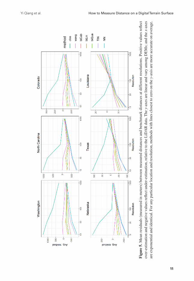
Yi Qiang et al How to Measure Distance on a Digital Terrain Surface
11
Fig
ure
5 M
ean
resi
dual
s (m
easu
red
in m
eter
s) b
etw
een
mea
sure
d di
stan
ces
and
benc
hmar
k di
stan
ces
at d
iffe
rent
res
olut
ions
Pos
itive
val
ues
refle
ct
over
-est
imat
ion
and
nega
tive
valu
es re
flect
und
er-e
stim
atio
n re
lativ
e to
the
LiD
AR
dat
a T
he y
-axe
s ar
e lin
ear a
nd v
ary
amon
g D
EM
s a
nd th
e x-
axes
ar
e ex
pone
ntia
l and
iden
tical
For
any
par
ticul
ar lo
catio
n an
d re
solu
tion
met
hods
with
line
s cl
oses
t to
zero
on
the
y-ax
is a
re m
ore
accu
rate
on
aver
age
Geographical Analysis
12
Fig
ure
6 M
ean
resi
dual
rat
ios
betw
een
benc
hmar
k di
stan
ces
and
mea
sure
d di
stan
ces
mea
sure
d at
dif
fere
nt r
esol
utio
ns P
ositi
ve v
alue
s re
flect
ove
r-es
timat
ion
and
nega
tive
valu
es r
eflec
t und
er-e
stim
atio
n r
elat
ive
to th
e L
iDA
R d
ata
Not
e th
at th
e y-
axes
dif
fer
acro
ss D
EM
s w
hile
the
x-ax
es a
re
cons
iste
nt a
nd lo
gari
thm
ical
ly r
esca
led
Yi Qiang et al How to Measure Distance on a Digital Terrain Surface
13
changing pattern of the ratios of residuals at different resolutions are analogous to the patterns of residuals shown in Fig 5 As shown in Fig 6 the error ratio of distance measurement for any given transect may range from minus2 to +4 depending on the surface-adjusted method the study area and on the resolution of the DEM Comparing among the study areas Louisiana has the smallest error magnitude with residual ratios ranging from ndash01 to 03 while the residual ratios in Colorado span ranging from minus02 to 27 indicating that distance measurement error tends to be larger in mountainous or uneven terrains than in flatter or smoother terrains
RMSE analysisRoot-Mean-Square Error (RMSE) indicates the absolute fit between measured distances and benchmark distances The RMSEs in Fig 7 generally confirm the patterns of residuals in Figs 5 and 6 with some interesting cross scale patterns highlighted RMSE values tend to rise as pixel size increases from 100 m with RMSE increasing for North Carolina and Colorado for 30 m and larger pixels Method-specific errors show greatest differences at finer resolutions resolv-ing to a value ranging between roughly 450 m (Nebraska) and 600 m (all other study areas) at 1000 m resolution The range of average error among methods is higher for mountainous and hilly landscapes with almost no difference among methods for the two flattest landscapes (Texas and Louisiana) The Weighted Average method generates the lowest RMSE magnitudes overall although the Closest Centroid method gives lower RMSE values at 100 m resolution for reasons that are not clear The bilinear method has the lowest RMSE of all three polynomial methods followed by the biquadratic and bicubic method
Processing timeProcessing time of the distance calculation increases at finer resolutions (ie as cell size de-creases) (Fig 8) TIN and Nearest Neighbor require the longest processing times except for North Carolina at 10 m resolution Shortest processing times are used by Weighted Average and Closest Centroid followed by the bilinear polynomial Processing times drop considerably for coarser resolution DEMs because of relatively fewer pixels Considering the changing patterns of residuals and RMSEs however there is a trade-off between accuracy and computational efficiency
Comparing among the different methods the Natural Neighbor and TIN method require the longest processing time in most landscapes Given their high residuals and RMSEs these two methods seem the least optimal for surface-adjusted distance calculation And while the Closest Centroid method takes the shortest processing time the accuracy metrics indicate that its utility for surface-adjusted distance estimation is highly varied and thus not consistently reliable The bilinear polynomial method gives more accurate estimations but takes additional processing time especially at fine resolutions Given the low absolute residuals and RMSEs in most landscapes and at most resolutions the weighted average method can be considered the sur-face adjusting method that best balances accuracy with processing time for distance calculation
Discussion and implications
This study applies a HPC-enabled Monte-Carlo simulation to evaluate seven surface adjustment methods for distance calculation on digital terrain Distances of 1000 randomly generated tran-sects were calculated in six study areas using different surface adjusting methods and DEMs at different resolutions The calculated distances were compared with benchmark distances
Geographical Analysis
14
Fig
ure
7 R
MSE
(m
easu
red
in m
eter
s) b
etw
een
benc
hmar
k di
stan
ces
and
mea
sure
d di
stan
ces
mea
sure
d in
dif
fere
nt r
esol
utio
ns N
ote
that
the
y-ax
es
are
scal
ed d
iffe
rent
ly a
cros
s pa
nels
Yi Qiang et al How to Measure Distance on a Digital Terrain Surface
15
Fig
ure
8 M
ean
proc
essi
ng ti
mes
(mea
sure
d in
sec
onds
) for
sur
face
-adj
uste
d di
stan
ce c
alcu
latio
n pe
r tra
nsec
t usi
ng d
iffe
rent
met
hods
and
at d
iffe
rent
re
solu
tions
Not
e th
at y
-axi
s va
lues
dif
fer
amon
g D
EM
s w
hile
x-a
xis
valu
es a
re id
entic
al
Geographical Analysis
16
measured on 3 m resolution DEMs to evaluate their accuracies Residuals and RMSEs compared measured distances with LiDAR benchmark distances To reduce the overall computing time the distance calculation algorithm was optimized to reduce memory usage and processing time in a multi-core computer
The major findings in this study include (1) the distance measurement varies with DEM res-olutions surface adjustment methods and terrain types (2) Weighted Average is overall the most accurate surface adjustment for distance measurement with a few exceptions (3) there is a trade-off between DEM resolution and computing time The assessment results provide a foundation for distance-based spatial analyses on terrain surface (eg distance-based point pattern analysis and kriging interpolation) In a broader sense the study increases the understanding about the interplay between analytic methods scale and the geographical phenomena being studied
The assessment reveals the dependency of distance measurement on data resolution surface adjustment methods and terrain variations The results show a pattern of distance underestimation relative to the LiDAR benchmarks at finer resolutions (10 m and 30 m) that transitions to near equivalence or slight overestimation as pixel size increases The degree of underestimation varies with method of surface adjustment The weighted average method has the highest accuracy overall in most situations This finding may seem surprising given that the method utilizes a search neigh-borhood of only 8 adjacent pixels In terrain with high local relief one might expect that the polyno-mial methods would provide better results due to larger neighborhoods andor adjustment methods that could filter localized perturbations in elevation The results indicate that biquadratic (8 neigh-bors) and the bicubic (16 neighbors) methods tend to exaggerate underestimation While the bilinear neighborhood (4 pixels) produces residuals and RMSE values closer to the weighted average the kernel is rarely centered on the point being adjusted and this can over- or underemphasize nearby terrain nonuniformity Closest Centroid TIN and Nearest Neighbor employ even smaller neighbor-hoods (1 3 and up to 6 neighbors respectively) further exacerbating the problem Overestimation of surface-adjusted distance for all methods at 1000 m resolution may be associated with neigh-borhood bias as well the spatial extent of larger pixels may ignore local features at the same time as weighting more distant features (up to 4 8 or 16 kilometers away) in equal consideration The weighted average method adjustment is based on central tendency and qualified by inverse distance weighting which can offset the impacts of rough or uneven terrain in more distant pixels
The balance between improved accuracy and extra processing time is relevant from a prac-tical standpoint The DEMs tested here are probably too small to be useful for regional or conti-nental modeling as for example studies involving sea level rise earthquake damage or coastal storm events Even with high performance computing distance adjustment for larger study areas could require minutes or longer Moreover distance estimation is often the initial step and rarely the final product of spatial modeling The Closest Centroid method calculates distance based on elevation in rigid pixels which does not adjust the terrain surface using surrounding elevation values Thus the distance measurements of this method fluctuate at different resolutions due to the stair-step effect of DEM pixels As a consequence the method tends to over-estimate distance at finer resolutions due to including too many (small) pixels and to under-estimate distance at coarser resolutions due to averaging within large pixels Despite carrying the lowest processing time the accuracy of the Closest Centroid method should not be considered a good choice when trying to balance accuracy with processing times Higher processing times shown by TIN and Nearest Neighbor are coupled with reduced accuracy and no balance is achieved Polynomial adjustment by second and third order equations reflects similar results Given the second lowest processing time the weighted average method can be considered the optimal surface adjusting
Yi Qiang et al How to Measure Distance on a Digital Terrain Surface
17
method for distance calculation in most situations Adjustment using bilinear polynomial estima-tion can be considered an alternative with slightly less improvement in accuracy
The accuracy of the surface adjustment methods also varies in different terrain types The ac-curacy difference among methods is smallest in flat terrain such as Louisiana and Texas implying that for these terrain types the choice of surface adjustment for distance measurements matters less than for hilly and mountainous terrain Differences in error metrics for more mountainous or nonuniform terrains show greater variation especially at fine and intermediate resolutions mean-ing the choice of surface adjustment appears to have a greater impact on distance estimation in rougher terrain and at finer resolutions Error magnitudes begin to coalesce after 100 m resolution for all methods indicating that at some point the extra computations required for surface adjust-ment are simply not worth the potential improvement in accuracy Accuracy of surface-adjusted distance measurement is reduced in DEMs that contain a mix of terrain types with some flat and some hilly areas Future research must investigate the relationships between terrain roughness terrain uniformity and accuracy to better understand the full implication of these findings
As an additional note methods that perform best for distance calculation may or may not be optimal for other tasks such as estimating surface-adjusted elevation or area Ghandehari Buttenfield and Farmer (2019) demonstrate that linear and bilinear polynomials give slightly better accuracies for surface-adjusted estimation of point elevation on DEMs although errors for any method are quite small on the order of centimeter magnitudes for terrain measured in me-ters Their study shows however that errors for all methods increase in rough terrain This reflects earlier research by Shi and Tian (2006) and Schneider (2001) showing that errors in elevation estimation are more prominent in rough terrain Ghandehari and Buttenfield (2018) compare sur-face-adjusted methods for estimating pixel surface areas finding that while a bicubic polynomial estimation gives the highest accuracy relative to a 3 m LiDAR benchmark it carries unreason-ably high processing times They modify Jennessrsquo (2004) surface area estimation method and then apply bilinear polynomial estimation to achieve nearly equivalent accuracies to the bicubic method with processing times reduced by nearly 80 (Ghandehari 2019)
As the primary objective of the study is to evaluate and compare among surface adjustment methods the simulation program is implemented in a simple parallel model which effectively reduces the computing time to a manageable level The performance of the simulation can be further improved with finer grain parallelism architectures such as OpenMP and MPI Also the program can be further parallelized by including on-the-fly transect generation and buffer area extraction These optimization options will be explored in future experiments such as surface-ad-justed area calculation for a new variety of case studies
The title of this article raises the issue of why accurate distance measurements matters in geographical analysis There are several reasons First and as described at the beginning of the article distance metrics underlie many if not most simple and compound GIS analytic methods Second it stands to reason that inaccurate distances can propagate inaccuracies throughout the entire course of spatial modeling and confound any estimates related to terrain surfaces as for ex-ample glacial recession wetlands fragmentation freight routing or debris flow estimation Third digital terrain is one of the most frequently included data layers in spatial analyses Bolstad (2019 p 485) cites the influence of terrain characteristics on a broad set of environmental functions such as soil moisture agricultural yields sediment transport and construction costs Wilson (2012 p 107) explains the important impact of terrain ldquohellip in modulating the atmospheric geomor-phic hydrologic and ecological processes operating on or near the Earthrsquos surfacerdquo He refers to Hutchinson and Gallant (2000) in arguing that the terrain is so tightly coupled with these four
Geographical Analysis
18
families of processes that characterization of the terrain directly leads to and refines insights about the nature of the processes In a nutshell geospatial analytics cannot be accurate without accurate distance metrics And because most geographic and geomorphic processes depend partially or wholly upon the land surface on which they are situated distance measurements should be per-formed on the terrain surface ldquoas the horse runsrdquo instead of ldquoas the crow fliesrdquo
With the emergence of parallel processing and the increased availability of fine resolution terrain data surface-adjusted distance metrics are becoming an operational strategy that can improve the accuracy of many types of spatial modeling although results depend upon several factors (resolution terrain type and uniformity and surface adjustment method) Three of those factors have been examined here but this study has limitations that call for additional examina-tion and assessment The characterization of terrain uniformity must be examined more formally along with possible interaction among the factors analyzed in this article Additionally the opti-mal methods choices need to be further tested and validated by embedding the surface-adjusted distance metrics into more complex analytics For instance a hypothesis to be tested is whether surface-adjusted distance can increase the accuracy of kriging interpolation Surface adjustment also needs to be embedded in full-blown surface process models to understand them in analytic practice And finally the assessment of distance measurement shows that choosing an appropri-ate (not necessarily the finest) scale is important for spatial analysis and modeling Quattrochi and Goodchild (1997) suggest that geographical analyses should be conducted at the operational scale (also referred to by Montello (2001) as phenomenon scale) where the studied processes operate since slight changes in these processes can invoke pronounced changes in model results The results reported in this study reveal that the optimal DEM resolutions for distance mea-surement varies among different surface adjustment methods and terrain types Importantly the choice of a method may also depend upon task (measuring distance surface area or volume) As distance is the most fundamental metric for geographical analyses the knowledge generated in this study lays a foundation for developing scale-sensitive analysis tools on a terrain surface
Acknowledgment
The authors acknowledge excellent and constructive comments from reviewers which strength-ened the text
Funding information
This article is based on work supported by the US National Science under the Methodology Measurement amp Stats (MMS) Program (Award No 1853866) This article is also based on work that is part of the Data Harmonization Initiative at Earth Lab (httpswwwcolor adoeduearth lab) supported by an investment from the University of Colorado Grand Challenge Initiative Any opinions findings and conclusions or recommendations expressed in this material are those of the authors and do not necessarily reflect the views of the funding agencies
Appendix
This appendix documents the data sets and their download sources used for the experiments in the manuscript The exact specifications are included here in the interests of reproducible sci-ence so that interested readers can replicate the study using the same data sets
Yi Qiang et al How to Measure Distance on a Digital Terrain Surface
19
Benchmark LiDAR data
State Benchmark LiDAR datasets
Colorado 2010 South San Luis Lakes LidarNebraska 2009 Nebraska Department of Natural Resources (DNR) South Central
Nebraska LidarNorth Carolina 2003 North Carolina Floodplain Mapping Program (NCFMP) LidarTexas 2011 Texas Natural Resources Information System (TNRIS) Lidar Bell
Burnet and McLennan CountiesWashington 2006 USGS Lidar North Puget Sound WashingtonLouisiana 1999 Louisiana Lidar Project (1999ndash2008)
Tiles of 10 m DEMsThe following tiles are available to download in USGS TNM Download httpsviewernatio nalmapgovbasic
State Tiles of 10 m DEM
Colorado USGS NED ned19_n39x25_w106x25_co_arkansasvalley_2010 19 arc-second 2012 15 times 15 min IMGUSGS NED ned19_n39x00_w106x50_co_arkansasvalley_2010 19 arc-second 2012 15 times 15 min IMGUSGS NED ned19_n38x75_w106x00_co_arkansasvalley_2010 19 arc-second 2012 15 times 15 min IMGUSGS NED ned19_n39x50_w106x00_co_grandco_2010 19 arc-second 2011 15 times 15 min IMGUSGS NED ned19_n38x75_w106x50_co_arkansasvalley_2010 19 arc-second 2012 15 times 15 min IMGUSGS NED ned19_n38x25_w106x25_co_sanluisvalley_2011 19 arc-second 2012 15 times 15 min IMGUSGS NED ned19_n38x50_w106x00_co_arkansasvalley_2010 19 arc-second 2012 15 times 15 min IMGUSGS NED ned19_n38x25_w106x00_co_arkansasvalley_2010 19 arc-second 2012 15 times 15 min IMGUSGS NED ned19_n38x25_w106x25_co_arkansasvalley_2 010 19 arc-second 2012 15 times 15 min IMGUSGS NED ned19_n39x25_w106x50_co_arkansasvalley_2010 19 arc-second 2012 15 times 15 min IMGUSGS NED ned19_n38x25_w106x00_co_sanluisvalley_2011 19 arc-second 2012 15 times 15 min IMGUSGS NED ned19_n39x00_w106x00_co_arkansasvalley_2010 19 arc-second 2012 15 times 15 min IMGUSGS NED ned19_n39x50_w106x25_co_arkansasvalley_2010 19 arc-second 2012 15 times 15 min IMGUSGS NED ned19_n38x50_w106x25_co_arkansasvalley_2010 19 arc-second 2012 15 times 15 min IMGUSGS NED ned19_n38x25_w106x50_co_sanluisvalley_2011 19 arc-second 2012 15 times 15 min IMG
Geographical Analysis
20
State Tiles of 10 m DEM
USGS NED ned19_n39x50_w106x50_co_arkansasvalley_2010 19 arc-second 2012 15 times 15 min IMGUSGS NED ned19_n38x75_w106x25_co_arkansasvalley_2010 19 arc-second 2012 15 times 15 min IMGUSGS NED ned19_n39x00_w106x25_co_arkansasvalley_2010 19 arc-second 2012 15 times 15 min IMGUSGS NED ned19_n38x25_w105x75_co_sanluisvalley_2011 19 arc-second 2012 15 times 15 min IMGUSGS NED ned19_n39x75_w106x00_co_grandco_2010 19 arc-second 2011 15 times 15 min IMGUSGS NED ned19_n38x00_w106x25_co_sanluisvalley_2011 19 arc-second 2012 15 times 15 min IMGUSGS NED ned19_n38x00_w106x00_co_sanluisvalley_2011 19 arc-second 2012 15 times 15 min IMGUSGS NED ned19_n38x00_w106x50_co_sanluisvalley_2011 19 arc-second 2012 15 times 15 min IMGUSGS NED ned19_n38x00_w105x75_co_sanluisvalley_2011 19 arc-second 2012 15 times 15 min IMG
Nebraska USGS NED ned19_n40x50_w100x25_ne_rainwater_2009 19 arc-second 2011 15 times 15 min IMGUSGS NED ned19_n40x50_w100x00_ne_rainwater_2009 19 arc-second 2011 15 times 15 min IMGUSGS NED ned19_n40x50_w100x50_ne_rainwater_2009 19 arc-second 2011 15 times 15 min IMGUSGS NED ned19_n40x75_w100x75_ne_rainwater_2009 19 arc-second 2011 15 times 15 min IMGUSGS NED ned19_n40x75_w100x00_ne_rainwater_2009 19 arc-second 2011 15 times 15 min IMGUSGS NED ned19_n40x75_w100x25_ne_rainwater_2009 19 arc-second 2011 15 times 15 min IMGUSGS NED ned19_n40x75_w100x50_ne_rainwater_2009 19 arc-second 2011 15 times 15 min IMGUSGS NED ned19_n40x50_w100x75_ne_rainwater_2009 19 arc-second 2011 15 times 15 min IMGUSGS NED ned19_n40x75_w101x00_ne_rainwater_2009 19 arc-second 2011 15 times 15 min IMGUSGS NED ned19_n40x50_w101x00_ne_rainwater_2009 19 arc-second 2011 15 times 15 min IMGUSGS NED ned19_n40x25_w100x00_ne_rainwater_2009 19 arc-second 2011 15 times 15 min IMGUSGS NED ned19_n40x25_w100x50_ne_rainwater_2009 19 arc-second 2011 15 times 15 min IMGUSGS NED ned19_n40x25_w100x25_ne_rainwater_2009 19 arc-second 2011 15 times 15 min IMG
Yi Qiang et al How to Measure Distance on a Digital Terrain Surface
21
State Tiles of 10 m DEM
USGS NED ned19_n40x25_w100x75_ne_rainwater_2009 19 arc-second 2011 15 times 15 min IMGUSGS NED ned19_n41x00_w100x75_ne_rainwater_2009 19 arc-second 2011 15 times 15 min IMGUSGS NED ned19_n41x00_w100x00_ne_rainwater_2009 19 arc-second 2011 15 times 15 min IMGUSGS NED ned19_n41x00_w100x50_ne_rainwater_2009 19 arc-second 2011 15 times 15 min IMGUSGS NED ned19_n41x00_w100x25_ne_rainwater_2009 19 arc-second 2011 15 times 15 min IMGUSGS NED ned19_n40x75_w099x75_ne_rainwater_2009 19 arc-second 2011 15 times 15 min IMGUSGS NED ned19_n40x50_w099x75_ne_rainwater_2009 19 arc-second 2011 15 times 15 min IMGUSGS NED ned19_n40x25_w101x00_ne_rainwater_2009 19 arc-second 2011 15 times 15 min IMGUSGS NED ned19_n41x00_w101x00_ne_rainwater_2009 19 arc-second 2011 15 times 15 min IMGUSGS NED ned19_n40x25_w099x75_ne_rainwater_2009 19 arc-second 2011 15 times 15 min IMGUSGS NED ned19_n41x00_w099x75_ne_rainwater_2009 19 arc-second 2011 15 times 15 min IMG
North Carolina
USGS NED ned19_n36x00_w081x50_nc_statewide_2003 19 arc-second 2012 15 times 15 min IMGUSGS NED ned19_n36x00_w082x00_nc_statewide_2003 19 arc-second 2012 15 times 15 min IMGUSGS NED ned19_n36x00_w081x25_nc_statewide_2003 19 arc-second 2012 15 times 15 min IMGUSGS NED ned19_n36x00_w081x75_nc_statewide_2003 19 arc-second 2012 15 times 15 min IMGUSGS NED ned19_n36x00_w081x00_nc_statewide_2003 19 arc-second 2012 15 times 15 min IMGUSGS NED ned19_n36x00_w082x25_nc_statewide_2003 19 arc-second 2012 15 times 15 min IMGUSGS NED ned19_n35x75_w082x00_nc_statewide_2003 19 arc-second 2012 15 times 15 min IMGUSGS NED ned19_n35x75_w081x25_nc_statewide_2003 19 arc-second 2012 15 times 15 min IMGUSGS NED ned19_n35x75_w081x50_nc_statewide_2003 19 arc-second 2012 15 times 15 min IMGUSGS NED ned19_n35x75_w081x75_nc_statewide_2003 19 arc-second 2012 15 times 15 min IMGUSGS NED ned19_n35x75_w081x00_nc_statewide_2003 19 arc-second 2012 15 times 15 min IMG
Geographical Analysis
22
State Tiles of 10 m DEM
USGS NED ned19_n35x75_w082x25_nc_statewide_2003 19 arc-second 2012 15 times 15 min IMGUSGS NED ned19_n36x25_w081x50_nc_statewide_2003 19 arc-second 2012 15 times 15 min IMGUSGS NED ned19_n36x25_w081x00_nc_statewide_2003 19 arc-second 2012 15 times 15 min IMGUSGS NED ned19_n36x25_w081x25_nc_statewide_2003 19 arc-second 2012 15 times 15 min IMGUSGS NED ned19_n36x25_w082x00_nc_statewide_2003 19 arc-second 2012 15 times 15 min IMGUSGS NED ned19_n36x25_w081x75_nc_statewide_2003 19 arc-second 2012 15 times 15 min IMGUSGS NED ned19_n36x25_w082x25_nc_statewide_2003 19 arc-second 2012 15 times 15 min IMGUSGS NED ned19_n36x00_w080x75_nc_statewide_2003 19 arc-second 2012 15 times 15 min IMGUSGS NED ned19_n35x75_w080x75_nc_statewide_2003 19 arc-second 2012 15 times 15 min IMGUSGS NED ned19_n36x25_w080x75_nc_statewide_2003 19 arc-second 2012 15 times 15 min IMG
Texas USGS NED ned19_n31x50_w097x50_tx_bellburnetmclennancos_2011 19 arc-second 2012 15 times 15 min IMGUSGS NED ned19_n31x25_w097x25_tx_bellburnetmclennancos_2011 19 arc-second 2012 15 times 15 min IMGUSGS NED ned19_n31x00_w098x25_tx_bellburnetmclennancos_2011 19 arc-second 2012 15 times 15 min IMGUSGS NED ned19_n31x25_w097x50_tx_bellburnetmclennancos_2011 19 arc-second 2012 15 times 15 min IMGUSGS NED ned19_n31x50_w097x75_tx_bellburnetmclennancos_2011 19 arc-second 2012 15 times 15 min IMGUSGS NED ned19_n31x75_w097x25_tx_bellburnetmclennancos_2011 19 arc-second 2012 15 times 15 min IMGUSGS NED ned19_n31x25_w098x25_tx_bellburnetmclennancos_2011 19 arc-second 2012 15 times 15 min IMGUSGS NED ned19_n31x00_w098x00_tx_bellburnetmclennancos_2011 19 arc-second 2012 15 timestimes 15 min IMGUSGS NED ned19_n31x25_w097x75_tx_bellburnetmclennancos_2011 19 arc-second 2012 15 times 15 min IMGUSGS NED ned19_n31x00_w097x50_tx_bellburnetmclennancos_2011 19 arc-second 2012 15 times 15 min IMGUSGS NED ned19_n31x00_w097x75_tx_bellburnetmclennancos_2011 19 arc-second 2012 15 times 15 min IMGUSGS NED ned19_n31x75_w097x50_tx_bellburnetmclennancos_2011 19 arc-second 2012 15 times 15 min IMG
Yi Qiang et al How to Measure Distance on a Digital Terrain Surface
23
State Tiles of 10 m DEM
USGS NED ned19_n31x25_w098x00_tx_bellburnetmclennancos_2011 19 arc-second 2012 15 times 15 min IMGUSGS NED ned19_n31x00_w097x25_tx_bellburnetmclennancos_2011 19 arc-second 2012 15 times 15 min IMGUSGS NED ned19_n31x50_w097x25_tx_bellburnetmclennancos_2011 19 arc-second 2012 15 times 15 min IMGUSGS NED ned19_n30x75_w098x25_tx_bellburnetmclennancos_2011 19 arc-second 2012 15 times 15 min IMGUSGS NED ned19_n30x75_w098x00_tx_bellburnetmclennancos_2011 19 arc-second 2012 15 times 15 min IMGUSGS NED ned19_n30x75_w097x50_tx_bellburnetmclennancos_2011 19 arc-second 2012 15 times 15 min IMGUSGS NED ned19_n30x75_w098x00_tx_central_llano_2007 19 arc-second 2010 15 times 15 min IMGUSGS NED ned19_n30x75_w098x25_tx_central_llano_2007 19 arc-second 2010 15 times 15 min IMGUSGS NED ned19_n31x75_w097x00_tx_bellburnetmclennancos_2011 19 arc-second 2012 15 times 15 min IMGUSGS NED ned19_n31x50_w097x00_tx_bellburnetmclennancos_2011 19 arc-second 2012 15 times 15 min IMGUSGS NED ned19_n31x25_w098x50_tx_central_llano_2007 19 arc-second 2010 15 times 15 min IMGUSGS NED ned19_n31x50_w098x50_tx_central_llano_2007 19 arc-second 2010 15 times 15 min IMGUSGS NED ned19_n31x00_w098x50_tx_central_llano_2007 19 arc-second 2010 15 times 15 min IMGUSGS NED ned19_n31x75_w098x50_tx_central_llano_2007 19 arc-second 2010 15 times 15 min IMGUSGS NED ned19_n31x00_w098x50_tx_bellburnetmclennancos_2011 19 arc-second 2012 15 times 15 min IMGUSGS NED ned19_n30x75_w098x50_tx_central_llano_2007 19 arc-second 2010 15 times 15 min IMGUSGS NED ned19_n30x75_w098x50_tx_bellburnetmclennancos_2011 19 arc-second 2012 15 times 15 min IMG
Washington USGS NED ned19_n48x50_w122x00_wa_northpugetsound_2006 19 arc-second 2009 15 times 15 min IMGUSGS NED ned19_n48x50_w122x50_wa_puget_sound_2000 19 arc-second 2012 15 times 15 min IMGUSGS NED ned19_n48x50_w121x50_wa_northpugetsound_2006 19 arc-second 2009 15 times 15 min IMGUSGS NED ned19_n49x00_w122x50_wa_northpugetsound_2006 19 arc-second 2009 15 times 15 min IMGUSGS NED ned19_n48x75_w122x75_wa_sanjuanco_2009 19 arc-second 2011 15 times 15 min IMG
Geographical Analysis
24
State Tiles of 10 m DEM
USGS NED ned19_n48x50_w122x25_wa_northpugetsound_2006 19 arc-second 2009 15 times 15 min IMGUSGS NED ned19_n48x75_w121x25_wa_northpugetsound_2006 19 arc-second 2009 15 times 15 min IMGUSGS NED ned19_n49x00_w121x25_wa_northpugetsound_2006 19 arc-second 2009 15 times 15 min IMGUSGS NED ned19_n49x00_w122x00_wa_northpugetsound_2006 19 arc-second 2009 15 times 15 min IMGUSGS NED ned19_n48x50_w122x75_wa_puget_sound_2000 19 arc-second 2012 15 times 15 min IMGUSGS NED ned19_n48x75_w122x00_wa_northpugetsound_2006 19 arc-second 2009 15 times 15 min IMGUSGS NED ned19_n48x75_w122x75_wa_northpugetsound_2006 19 arc-second 2009 15 times 15 min IMGUSGS NED ned19_n48x75_w121x75_wa_northpugetsound_2006 19 arc-second 2009 15 times 15 min IMGUSGS NED ned19_n48x75_w122x25_wa_northpugetsound_2006 19 arc-second 2009 15 times 15 min IMGUSGS NED ned19_n49x00_w121x75_wa_northpugetsound_2006 19 arc-second 2009 15 times 15 min IMGUSGS NED ned19_n48x75_w122x50_wa_northpugetsound_2006 19 arc-second 2009 15 times 15 min IMGUSGS NED ned19_n49x00_w122x25_wa_northpugetsound_2006 19 arc-second 2009 15 times 15 min IMGUSGS NED ned19_n48x50_w122x50_wa_northpugetsound_2006 19 arc-second 2009 15 times 15 min IMGUSGS NED ned19_n48x50_w122x75_wa_northpugetsound_2006 19 arc-second 2009 15 times 15 min IMGUSGS NED ned19_n48x75_w121x50_wa_northpugetsound_2006 19 arc-second 2009 15 times 15 min IMGUSGS NED ned19_n49x00_w122x75_wa_northpugetsound_2006 19 arc-second 2009 15 times 15 min IMGUSGS NED ned19_n48x50_w121x75_wa_northpugetsound_2006 19 arc-second 2009 15 times 15 min IMGUSGS NED ned19_n49x25_w122x25_wa_northpugetsound_2006 19 arc-second 2009 15 times 15 min IMGUSGS NED ned19_n49x25_w122x50_wa_northpugetsound_2006 19 arc-second 2009 15 times 15 min IMGUSGS NED ned19_n49x25_w122x00_wa_northpugetsound_2006 19 arc-second 2009 15 times 15 min IMGUSGS NED ned19_n49x25_w122x75_wa_northpugetsound_2006 19 arc-second 2009 15 times 15 min IMGUSGS NED ned19_n48x25_w122x50_wa_puget_sound_2000 19 arc-second 2012 15 times 15 min IMG
Yi Qiang et al How to Measure Distance on a Digital Terrain Surface
25
State Tiles of 10 m DEM
USGS NED ned19_n48x25_w122x75_wa_puget_sound_2000 19 arc-second 2012 15 times 15 min IMGUSGS NED ned19_n48x50_w123x00_wa_puget_sound_2000 19 arc-second 2012 15 times 15 min IMGUSGS NED ned19_n48x75_w123x00_wa_sanjuanco_2009 19 arc-second 2011 15 times 15 min IMGUSGS NED ned19_n49x00_w123x00_wa_northpugetsound_2006 19 arc-second 2009 15 times 15 min IMGUSGS NED ned19_n48x50_w123x00_wa_sanjuanco_2009 19 arc-second 2011 15 times 15 min IMGUSGS NED ned19_n49x25_w123x00_wa_northpugetsound_2006 19 arc-second 2009 15 times 15 min IMGUSGS NED ned19_n48x25_w123x00_wa_puget_sound_2000 19 arc-second 2012 15 times 15 min IMG
Louisiana USGS NED ned19_n30x75_w091x50_la_statewide_2006 19 arc-second 2009 15 times 15 min IMGUSGS NED ned19_n30x50_w091x00_la_statewide_2006 19 arc-second 2009 15 times 15 min IMGUSGS NED ned19_n30x50_w091x50_la_atchafalayabasin_2010 19 arc-second 2011 15 times 15 min IMGUSGS NED ned19_n30x50_w091x50_la_statewide_2006 19 arc-second 2009 15 times 15 min IMGUSGS NED ned19_n30x75_w091x00_la_statewide_2006 19 arc-second 2009 15 times 15 min IMGUSGS NED ned19_n30x75_w091x25_la_statewide_2006 19 arc-second 2009 15 times 15 min IMGUSGS NED ned19_n30x75_w090x75_la_statewide_2006 19 arc-second 2009 15 times 15 min IMGUSGS NED ned19_n30x50_w091x25_la_statewide_2006 19 arc-second 2009 15 times 15 min IMGUSGS NED ned19_n30x50_w090x75_la_statewide_2006 19 arc-second 2009 15 times 15 min IMGUSGS NED ned19_n30x50_w091x50_LA-USGS_Atchafalaya2_2012_2014 19 arc-second 20140615 15 15 min IMGUSGS NED ned19_n31x00_w091x50_la_statewide_2006 19 arc-second 2009 15 times 15 min IMGUSGS NED ned19_n31x00_w091x25_la_statewide_2006 19 arc-second 2009 15 times 15 min IMGUSGS NED ned19_n31x00_w091x00_la_statewide_2006 19 arc-second 2009 15 times 15 min IMGUSGS NED ned19_n31x00_w090x75_la_statewide_2006 19 arc-second 2009 15 times 15 min IMGUSGS NED ned19_n30x25_w091x00_la_statewide_2006 19 arc-second 2009 15 times 15 min IMG
Geographical Analysis
26
State Tiles of 10 m DEM
USGS NED ned19_n30x25_w091x50_la_atchafalayabasin_2010 19 arc-second 2011 15 times 15 min IMGUSGS NED ned19_n30x25_w091x50_la_statewide_2006 19 arc-second 2009 15 times 15 min IMGUSGS NED ned19_n30x25_w090x75_la_statewide_2006 19 arc-second 2009 15 times 15 min IMGUSGS NED ned19_n30x25_w091x25_la_statewide_2006 19 arc-second 2009 15 times 15 min IMGUSGS NED ned19_n30x25_w091x50_LA-USGS_Atchafalaya2_2012_2014 19 arc-second 20140615 15 times 15 min IMGUSGS NED ned19_n30x25_w091x25_LA-USGS_Atchafalaya2_2012_2014 19 arc-second 20140615 15 times 15 min IMGUSGS NED ned19_n30x75_w090x50_la_statewide_2006 19 arc-second 2009 15 times 15 min IMGUSGS NED ned19_n30x50_w090x50_la_statewide_2006 19 arc-second 2009 15 times 15 min IMGUSGS NED ned19_n30x75_w091x75_la_statewide_2006 19 arc-second 2009 15 times 15 min IMGUSGS NED ned19_n30x50_w091x75_la_atchafalayabasin_2010 19 arc-second 2011 15 times 15 min IMGUSGS NED ned19_n30x50_w091x75_la_statewide_2006 19 arc-second 2009 15 times 15 min IMGUSGS NED ned19_n30x75_w091x75_la_atchafalayabasin_2010 19 arc-second 2011 15 times 15 min IMGUSGS NED ned19_n30x75_w091x75_LA-USGS_Atchafalaya2_2012_2014 19 arc-second 20140615 15 times 15 min IMGUSGS NED ned19_n30x50_w091x75_LA-USGS_Atchafalaya2_2012_2014 19 arc-second 20140615 15 times 15 min IMGUSGS NED ned19_n31x00_w090x50_la_statewide_2006 19 arc-second 2009 15 times 15 min IMGUSGS NED ned19_n30x25_w090x50_la_statewide_2006 19 arc-second 2009 15 times 15 min IMGUSGS NED ned19_n31x00_w091x75_la_statewide_2006 19 arc-second 2009 15 times 15 min IMGUSGS NED ned19_n31x00_w091x75_LA-USGS_Atchafalaya2_2012_2014 19 arc-second 20140615 15 times 15 min IMGUSGS NED ned19_n30x25_w091x75_la_atchafalayabasin_2010 19 arc-second 2011 15 times 15 min IMGUSGS NED ned19_n30x25_w091x75_la_statewide_2006 19 arc-second 2009 15 times 15 min IMGUSGS NED ned19_n30x25_w091x75_LA-USGS_Atchafalaya2_2012_2014 19 arc-second 20140615 15 times 15 min IMG
Tiles of 30 m DEMs
Yi Qiang et al How to Measure Distance on a Digital Terrain Surface
27
The following tiles are available to download in USGS TNM Download httpsviewernatio nalmapgovbasic
State Tiles of 30 m DEM
Colorado USGS NED 13 arc-second n40w107USGS NED n39w107 13 arc-secondUSGS NED 13 arc-second n40w106USGS NED 13 arc-second n39w106
Nebraska USGS NED 13 arc-second n41w101 1 x 1 degree ArcGrid 2019USGS NED 13 arc-second n41w100 1 x 1 degree ArcGrid 2019
North Carolina USGS NED 13 arc-second n36w082 1 x 1 degree ArcGrid 2019USGS NED n36w081 13 arc-second 2013 1 x 1 degree ArcGridUSGS NED 13 arc-second n36w083 1 x 1 degree ArcGrid 2017USGS NED 13 arc-second n37w082 1 x 1 degree ArcGrid 2019USGS NED 13 arc-second n37w081 1 x 1 degree ArcGrid 2018USGS NED 13 arc-second n37w083 1 x 1 degree ArcGrid 2018
Texas USGS NED 13 arc-second n32w098 1 x 1 degree ArcGrid 2019USGS NED 13 arc-second n31w098 1 x 1 degree ArcGrid 2019USGS NED 13 arc-second n32w099 1 x 1 degree ArcGrid 2019USGS NED 13 arc-second n31w099 1 x 1 degree ArcGrid 2019USGS NED 13 arc-second n32w097 1 x 1 degree ArcGrid 2019USGS NED 13 arc-second n31w097 1 x 1 degree ArcGrid 2019
Washington USGS NED 13 arc-second n49w122 1 x 1 degree ArcGrid 2018USGS NED 13 arc-second n49w123 1 x 1 degree ArcGrid 2019USGS NED 13 arc-second n50w122 1 x 1 degree ArcGrid 2018USGS NED 13 arc-second n49w121 1 x 1 degree ArcGrid 2018USGS NED 13 arc-second n50w123 1 x 1 degree ArcGrid 2018
Louisiana USGS NED 13 arc-second n31w091 1 x 1 degree ArcGrid 2019USGS NED 13 arc-second n31w092 1 x 1 degree ArcGrid 2019
Tiles of 100 m and 1000 m DEMsThe following tiles are available to download in USGSrsquos website httpsddscrusgsgovsrtmversi on2_1
States Tiles 100 m DEM Tiles 1000 m DEM
Colorado N38W107SRTMGL3 w140n40SRTM30N39W107SRTMGL3N39W106SRTMGL3N38W106SRTMGL3
Nebraska N40W100SRTMGL3 w140n90SRTM30N40W101SRTMGL3
North Carolina N35W082SRTMGL3 w140n90SRTM30N35W081SRTMGL3N35W083SRTMGL3
Texas N29W098SRTMGL3N29W099SRTMGL3
Washington N48W123SRTMGL3 w100n40SRTM30N48W122SRTMGL3
Louisiana N29W091SRTMGL3 w100n40SRTM30N29W092SRTMGL3
Geographical Analysis
28
Tab
les
of
the
anal
ysis
res
ult
s
Tab
le A
1 R
esid
ual
Ave
rage
Res
idua
l R
MSE
and
Pro
cess
ing
Tim
e fo
r W
ashi
ngto
n I
nter
pola
tion
Met
hods
Inc
lude
(in
Top
-to-
Bot
tom
Ord
er)
Bic
ubic
Bili
near
and
Biq
uadr
atic
pol
ynom
ials
Clo
sest
Cen
troi
d N
eare
st N
eigh
bor
Tri
angu
late
d Ir
regu
lar
Net
wor
k a
nd W
eigh
ted
Ave
rage
Res
olut
ion
Stud
y ar
eaIn
terp
olat
ion
met
hod
Avg
res
idua
l (m
)A
vg t
ime
(s)
Avg
rat
io o
f re
sidu
alR
MSE
(m
)
10W
ashi
ngto
nbi
Cub
minus474
29
231
60minus0
016
0859
825
10W
ashi
ngto
nbi
Lin
minus275
87
210
59minus0
009
4235
463
10W
ashi
ngto
nbi
Qua
minus350
39
216
51minus0
011
9144
494
10W
ashi
ngto
ncl
os1
317
0319
142
004
514
166
534
10W
ashi
ngto
nN
Nminus8
785
922
620
minus00
2975
110
814
10W
ashi
ngto
nT
INminus7
763
841
305
minus00
2623
975
0410
Was
hing
ton
wav
g37
99
196
900
0013
599
64
30W
ashi
ngto
nbi
Cub
minus319
35
200
4minus0
010
8939
954
30W
ashi
ngto
nbi
Lin
minus136
67
117
3minus0
004
7117
310
30W
ashi
ngto
nbi
Qua
minus210
48
143
0minus0
007
1726
271
30W
ashi
ngto
ncl
os1
069
140
817
003
723
137
121
30W
ashi
ngto
nN
Nminus5
671
85
546
minus00
1943
722
4030
Was
hing
ton
TIN
minus476
51
113
48minus0
016
1159
879
30W
ashi
ngto
nw
avg
745
10
865
000
269
130
6510
0W
ashi
ngto
nbi
Cub
minus306
76
050
3minus0
010
5040
213
100
Was
hing
ton
biL
inminus1
754
80
273
minus00
0599
237
1110
0W
ashi
ngto
nbi
Qua
minus217
31
034
0minus0
007
2829
031
100
Was
hing
ton
clos
698
930
204
002
469
915
6410
0W
ashi
ngto
nN
Nminus4
112
01
650
minus00
1399
532
3210
0W
ashi
ngto
nT
INminus3
183
73
383
minus00
1065
416
4110
0W
ashi
ngto
nw
avg
minus22
260
201
minus00
0032
111
771
000
Was
hing
ton
biC
ubminus2
395
00
108
minus00
0719
548
591
000
Was
hing
ton
biL
inminus2
007
10
077
minus00
0754
516
001
000
Was
hing
ton
biQ
uaminus2
225
70
083
minus00
0850
543
431
000
Was
hing
ton
clos
299
990
068
001
204
578
811
000
Was
hing
ton
NN
minus223
18
014
7minus0
007
6052
918
100
0W
ashi
ngto
nT
INminus1
614
80
450
minus00
0758
471
211
000
Was
hing
ton
wav
gminus1
298
90
068
minus00
0484
496
20
Yi Qiang et al How to Measure Distance on a Digital Terrain Surface
29
Table A2 Residual Average Residual RMSE and Processing Time for North Carolina Interpolation Methods Include (in Top-to-Bottom Order) Bicubic Bilinear and Biquadratic polynomials Closest Centroid Nearest Neighbor Triangulated Irregular Network and Weighted Average
Resolution Study Area MethodAvg residual Avg time
Avg ratio of residual RMSE
10 North Carolina biCub minus39280 82186 minus000973 4971710 North Carolina biLin minus25592 78635 minus000643 3262710 North Carolina biQua minus30551 79250 minus000761 3872610 North Carolina clos 103191 75460 002535 13173110 North Carolina NN minus79594 34227 minus001958 10150610 North Carolina TIN minus75426 72281 minus001853 9519210 North Carolina wavg minus886 76333 minus000033 715030 North Carolina biCub minus36234 4078 minus000897 4675230 North Carolina biLin minus18032 2678 minus000452 2319130 North Carolina biQua minus25272 3131 minus000626 3251230 North Carolina clos 79456 1949 001972 10139030 North Carolina NN minus54725 10186 minus001360 7172030 North Carolina TIN minus52388 20687 minus001293 6667230 North Carolina wavg minus3793 2088 minus000093 6429100 North Carolina biCub minus38245 0921 minus000938 50519100 North Carolina biLin minus30836 0499 minus000754 40788100 North Carolina biQua minus33905 0624 minus000835 44764100 North Carolina clos 9981 0357 000278 19506100 North Carolina NN minus41975 2560 minus001046 55973100 North Carolina TIN minus39808 5935 minus000986 52072100 North Carolina wavg minus25205 0364 minus000618 330921000 North Carolina biCub minus13916 0122 minus000105 641361000 North Carolina biLin minus10973 0091 minus000167 623531000 North Carolina biQua minus14067 0096 minus000124 643461000 North Carolina clos minus5074 0083 minus000054 610341000 North Carolina NN minus14628 0120 minus000200 639841000 North Carolina TIN minus12287 0468 minus000255 623091000 North Carolina wavg minus13194 0081 minus000080 63061
Geographical Analysis
30
Table A3 Residual Average Residual RMSE and Processing Time for Colorado Interpolation Methods Include (in Top-to-Bottom Order) Bicubic Bilinear and Biquadratic Polynomials Closest Centroid Nearest Neighbor Triangulated Irregular Network and Weighted Average
Resolution Study Area Method Avg residual Avg timeAvg ratio of residual RMSE
10 Colorado biCub minus21068 7957 minus000968 2870810 Colorado biLin minus11997 5588 minus000566 1680410 Colorado biQua minus15591 6381 minus000729 2153010 Colorado clos 60424 4200 002749 7803210 Colorado NN minus35698 17031 minus001629 5060910 Colorado TIN minus42632 29384 minus001930 5665410 Colorado wavg 1410 4499 000046 585530 Colorado biCub minus18084 1800 minus000808 2462830 Colorado biLin minus8422 1095 minus000382 1198230 Colorado biQua minus12450 1309 minus000560 1721130 Colorado clos 45183 0729 002082 5887330 Colorado NN minus26450 3091 minus001182 3729630 Colorado TIN minus29240 7784 minus001326 3921530 Colorado wavg minus513 0798 minus000020 5506100 Colorado biCub minus18886 0520 minus000839 25817100 Colorado biLin minus13441 0311 minus000593 18908100 Colorado biQua minus15535 0367 minus000703 21444100 Colorado clos 16414 0208 000757 24211100 Colorado NN minus19998 0736 minus000922 28223100 Colorado TIN minus21186 2349 minus000992 28612100 Colorado wavg minus9335 0226 minus000413 143081000 Colorado biCub minus9685 0077 minus000350 630701000 Colorado biLin minus6277 0059 000636 633641000 Colorado biQua minus6457 0061 000222 586041000 Colorado clos minus911 0054 000077 597911000 Colorado NN minus9166 0078 000324 599841000 Colorado TIN minus8685 0234 minus000152 590841000 Colorado wavg minus3811 0054 000378 57750
Yi Qiang et al How to Measure Distance on a Digital Terrain Surface
31
Table A4 Residual Average Residual RMSE and Processing Time for Nebraska Interpolation Methods Include (in Top-to-Bottom Order) Bicubic Bilinear and Biquadratic polynomials Closest Centroid Nearest Neighbor Triangulated Irregular Network and Weighted Average
Resolution Study Area Method Avg residual Avg timeAvg ratio of residual RMSE
10 Nebraska biCub minus15507 15751 minus000438 1842310 Nebraska biLin minus8786 12139 minus000249 1051610 Nebraska biQua minus11645 13238 minus000329 1385010 Nebraska clos 36339 9779 001024 4281710 Nebraska NN minus24660 15574 minus000693 2919010 Nebraska TIN minus24193 35472 minus000681 2859210 Nebraska wavg minus1845 10406 minus000054 285030 Nebraska biCub minus12290 2861 minus000345 1480730 Nebraska biLin minus6632 1831 minus000187 812330 Nebraska biQua minus9544 2162 minus000269 1150730 Nebraska clos 23939 1287 000676 2831630 Nebraska NN minus15898 4681 minus000447 1896130 Nebraska TIN minus15391 10863 minus000436 1831230 Nebraska wavg minus3888 1374 minus000111 5014100 Nebraska biCub minus9337 0776 minus000268 12040100 Nebraska biLin minus7733 0470 minus000222 10434100 Nebraska biQua minus8326 0560 minus000232 11135100 Nebraska clos 1640 0330 000043 5837100 Nebraska NN minus10137 1126 minus000282 13097100 Nebraska TIN minus9717 3289 minus000271 12620100 Nebraska wavg minus6860 0341 minus000198 97011000 Nebraska biCub minus599 0131 000065 443391000 Nebraska biLin minus846 0090 000058 457281000 Nebraska biQua minus715 0098 000009 426081000 Nebraska clos 070 0076 minus000046 439671000 Nebraska NN minus2165 0120 minus000030 448871000 Nebraska TIN 049 0437 000077 452231000 Nebraska wavg minus658 0077 minus000055 44366
Geographical Analysis
32
Table A5 Residual Average Residual RMSE and Processing Time for Texas Interpolation Methods Include (in Top-to-Bottom Order) Bicubic Bilinear and Biquadratic Polynomials Closest Centroid Nearest Neighbor Triangulated Irregular Network and Weighted Average
Resolution Study Area Method Avg residual Avg timeAvg ratio of residual RMSE
10 Texas biCub minus6678 13527 minus000195 814210 Texas biLin minus4630 10210 minus000135 567810 Texas biQua minus5603 11303 minus000164 682910 Texas clos 10990 8228 000317 1408710 Texas NN minus9274 16384 minus000269 1155410 Texas TIN minus9619 34548 minus000280 1183410 Texas wavg minus2283 8734 minus000067 291030 Texas biCub minus4288 2730 minus000129 552930 Texas biLin minus2693 1761 minus000087 364330 Texas biQua minus3388 2076 minus000098 444730 Texas clos 7699 1241 000218 1039430 Texas NN minus5702 3433 minus000171 735530 Texas TIN minus5518 9743 minus000169 704430 Texas wavg minus1467 1330 minus000047 2510100 Texas biCub minus3155 0775 minus000107 6498100 Texas biLin minus2425 0481 minus000080 6196100 Texas biQua minus2945 0565 minus000079 6493100 Texas clos 4061 0338 000099 7431100 Texas NN minus3677 0815 minus000113 7056100 Texas TIN minus3622 3066 minus000121 7066100 Texas wavg minus1931 0355 minus000081 59641000 Texas biCub 929 0106 000991 601131000 Texas biLin 195 0078 001138 613451000 Texas biQua 870 0082 001353 622861000 Texas clos 220 0069 000922 616651000 Texas NN 2542 0097 000987 610911000 Texas TIN minus1579 0339 000748 633421000 Texas wavg minus218 0069 000829 61030
Yi Qiang et al How to Measure Distance on a Digital Terrain Surface
33
Table A6 Residual Average Residual RMSE and Processing Time for Louisiana Interpolation Methods Include (in top-to-bottom order) Bicubic Bilinear and Biquadratic polynomials Closest Centroid Nearest Neighbor Triangulated Irregular Network and Weighted Average
Resolution Study Area Method Avg residual Avg timeAvg ratio of residual RMSE
10 Louisiana biCub minus3132 25881 minus000084 384410 Louisiana biLin minus2262 22476 minus000061 279310 Louisiana biQua minus2722 23573 minus000073 334310 Louisiana clos 2551 19252 000070 318010 Louisiana NN minus3294 27879 minus000088 402610 Louisiana TIN minus3380 51336 minus000091 411510 Louisiana wavg minus1800 20357 minus000048 222330 Louisiana biCub minus1636 2924 minus000048 257630 Louisiana biLin minus1284 1806 minus000036 220030 Louisiana biQua minus1501 2171 minus000042 248230 Louisiana clos 486 1288 000013 175630 Louisiana NN minus1645 7183 minus000045 258830 Louisiana TIN minus1642 14367 minus000046 256330 Louisiana wavg minus1154 1367 minus000030 2129100 Louisiana biCub minus706 0792 minus000014 5329100 Louisiana biLin minus818 0492 minus000019 5458100 Louisiana biQua minus532 0579 minus000017 5348100 Louisiana clos minus543 0330 minus000003 5361100 Louisiana NN minus789 0772 minus000020 5375100 Louisiana TIN minus916 3179 minus000025 5644100 Louisiana wavg minus640 0361 minus000009 55851000 Louisiana biCub 494 0109 000265 584241000 Louisiana biLin 1730 0079 000215 593021000 Louisiana biQua 839 0084 000325 613951000 Louisiana clos 744 0067 000203 603861000 Louisiana NN minus119 0112 000123 602791000 Louisiana TIN 1416 0369 000168 599011000 Louisiana wavg 1211 0070 000236 59514
Geographical Analysis
34
References
Bolstad P (2019) GIS Fundamentals A First Text on Geographic Information systems 6th ed Ann Arbor MI XanEdu Publishing Inc
Buttenfield B M Ghandehari S Leyk L Stanislawski M Brantley Y Qiang (2016) Measuring Distance ldquoAs the Horse Runsrdquo Cross-Scale Comparison of Terrain-Based Metrics International Conference on GIScience Short Paper Proceedings 1 httpdxdoiorg1021433 b3118 rh987cz
Chang K and B Tsai (1991) ldquoThe Effect of DEM Resolution on Slope and Aspect Mappingrdquo Cartography and Geographic Information Systems 18(1) 69ndash77 httpsdoiorg10155915230 40917 83805626
GDALOGR contributors (2020) GDALOGR GEOSPATIAL Data Abstraction Software Library Open Source Geospatial Foundation httpsgdalorg
Gesch D B (2007) ldquoThe National Elevation Datasetrdquo In Digital Elevation Model Technologies and Applications The DEM Users Manual 2nd ed 99ndash118
Gesch DB M J Oimoen and G A Evans (2014) ldquoAccuracy Assessment of the US Geological Survey National Elevation Dataset and Comparison with Other Large-Area Elevation Datasets SRTM and ASTERrdquo Report No 2014ndash1008 Open-File Report p 18 USGS Publications Warehouse httpsdoiorg103133ofr20 141008
Ghandehari M (2019) Cross-Scale Analysis of Surface-Adjusted Measurements in digital Elevation Models Doctoral dissertation University of Colorado Boulder
Ghandehari M and B Buttenfield (2018) ldquoSlope-Adjusted Surface Area Computations in Digital Terrainrdquo Proceedings of 5th International Conference of the International Society of Geomorphometry (Geomorphometry 2018)
Ghandehari M B P Buttenfield C J Q Farmer (2019) Comparing the accuracy of estimated terrain elevations across spatial resolution International Journal of Remote Sensing 40(13) 5025ndash5049 httpdxdoiorg10108001431 16120191577581
Gutieacuterrez M (2012) ldquoChapter 153 Applied Geomorphology in Periglacial Reginsrdquo In Geomorphology 601ndash13 Boca Raton FL Taylor amp Francis
Harms T K E A Wentz and N B Grimm (2009) ldquoSpatial Heterogeneity of Denitrification in Semi-Arid Floodplainsrdquo Ecosystems 12(1) 129ndash43 httpsdoiorg101007s1002 1-008-9212-6
Hutchinson M F and J C Gallant (2000) Digital Elevation Models and Representation of Terrain Shape httpspubli catio nscsiroaurprpublist=BROamppid=proci te46f1d e5d-172e-4f8e-8696-da3b6 f7b03ca
Jenness J S (2004) ldquoCalculating Landscape Surface Area from Digital Elevation Modelsrdquo Wildlife Society Bulletin 32(3) 829ndash39 httpsdoiorg1021930091-7648(2004)032[0829CLSAF D]20CO2
Kienzle S (2004) ldquoThe Effect of DEM Raster Resolution on First Order Second Order and Compound Terrain Derivativesrdquo Transactions in GIS 8(1) 83ndash111 httpsdoiorg101111j1467-9671200400169x
Kiessling F P Nefzger J Nolasco and U Kaintzyk (2014) Overhead Power Lines Planning Design Construction Berlin Germany Springer
Montello D R (2001) ldquoScale in Geographyrdquo In International Encyclopedia of the Social and Behavioral Sciences 13501ndash4 edited by N J Smelser and B Baltes
Oliphant T E (2006) A guide to NumPy (Vol 1) Trelgol Publishing USAQiang Y B P Buttenfield N Lam and N V de Weghe (2018) ldquoNovel Models for Multi-Scale Spatial
and Temporal Analysesrdquo In 10th International Conference on Geographic Information Science (GIScience 2018) Vol 114 551ndash557 edited by S Winter A Griffin amp M Sester Dagstuhl Germany Schloss DagstuhlndashLeibniz-Zentrum fuer Informatik httpsdoiorg104230LIPIcsGISCI ENCE201855
Qiang Y and N Van de Weghe (2019) ldquoRe-Arranging Space Time and Scales in GIS Alternative Models for Multi-Scale Spatio-Temporal Modeling and Analysesrdquo ISPRS International Journal of Geo-Information 8(2) 72 httpsdoiorg103390ijgi8 020072
Quattrochi D A and M F Goodchild (1997) Scale in Remote Sensing and GIS Boca Raton FL CRC Press
Schneider B (2001) On the Uncertainty of Local Shape of Lines and Surfaces Cartography and Geographic Information Science 28(4) 237ndash247 httpsdoiorg10155915230 40017 82152991
Yi Qiang et al How to Measure Distance on a Digital Terrain Surface
35
Shafique M M van der Meijde N Kerle and F van der Meer (2011) ldquoImpact of DEM Source and Resolution on Topographic Seismic Amplificationrdquo International Journal of Applied Earth Observation and Geoinformation 13(3) 420ndash7 httpsdoiorg101016jjag201009005
Shi W Z and Y Tian (2006) ldquoA Hybrid Interpolation Method for the Refinement of a Regular Grid Digital Elevation Modelrdquo International Journal of Geographical Information Science 20(1) 53ndash67 httpsdoiorg10108013658 81050 0286943
Sibson R (1981) ldquoA Brief Description of Natural Neighbor Interpolationrdquo In Interpolating Multivariate Data 21ndash36 New York John Wiley amp Sons
Stanislawski L V J Falgout and B P Buttenfield (2015) ldquoAutomated Extraction of Natural Drainage Density Patterns for the Conterminous United States through High-Performance Computingrdquo The Cartographic Journal 52(2) 185ndash92 httpsdoiorg10108000087 04120151119466
Stoker J M (2018) The US Geological Survey Physical Scientist The Chief Elevation Scientist for the National Geospatial Program personal communication (jstokerusgsgov) [Personal communication]
The IPython Development Team (2018) Using IPython for parallel computing httpsipypa rallelreadt hedocsioenlates t
Tucker G E and G R Hancock (2010) ldquoModelling Landscape Evolutionrdquo Earth Surface Processes and Landforms 35(1) 28ndash50 httpsdoiorg101002esp1952
University Corporation for Atmospheric Research (UCAR) (2004) Natgrid Introduction httpwwwncargucaredungmat hnatgr idnnhomehtml
Usery E L M P Finn D J Scheidt S Ruhl T Beard and M Bearden (2004) ldquoGeospatial Data Resampling and Resolution Effects on Watershed Modeling A Case Study Using the Agricultural Non-Point Source Pollution Modelrdquo Journal of Geographical Systems 6(3) 289ndash306 httpsdoiorg101007s1010 9-004-0138-z
Wilson J P (2012) ldquoDigital Terrain Modelingrdquo Geomorphology 137(1) 107ndash21 httpsdoiorg101016jgeomo rph201103012
Zhang W and D R Montgomery (1994) ldquoDigital Elevation Model Grid Size Landscape Representation and Hydrologic Simulationsrdquo Water Resources Research 30(4) 1019ndash28 httpsdoiorg10102993WR0 3553

Geographical Analysis
12
Fig
ure
6 M
ean
resi
dual
rat
ios
betw
een
benc
hmar
k di
stan
ces
and
mea
sure
d di
stan
ces
mea
sure
d at
dif
fere
nt r
esol
utio
ns P
ositi
ve v
alue
s re
flect
ove
r-es
timat
ion
and
nega
tive
valu
es r
eflec
t und
er-e
stim
atio
n r
elat
ive
to th
e L
iDA
R d
ata
Not
e th
at th
e y-
axes
dif
fer
acro
ss D
EM
s w
hile
the
x-ax
es a
re
cons
iste
nt a
nd lo
gari
thm
ical
ly r
esca
led
Yi Qiang et al How to Measure Distance on a Digital Terrain Surface
13
changing pattern of the ratios of residuals at different resolutions are analogous to the patterns of residuals shown in Fig 5 As shown in Fig 6 the error ratio of distance measurement for any given transect may range from minus2 to +4 depending on the surface-adjusted method the study area and on the resolution of the DEM Comparing among the study areas Louisiana has the smallest error magnitude with residual ratios ranging from ndash01 to 03 while the residual ratios in Colorado span ranging from minus02 to 27 indicating that distance measurement error tends to be larger in mountainous or uneven terrains than in flatter or smoother terrains
RMSE analysisRoot-Mean-Square Error (RMSE) indicates the absolute fit between measured distances and benchmark distances The RMSEs in Fig 7 generally confirm the patterns of residuals in Figs 5 and 6 with some interesting cross scale patterns highlighted RMSE values tend to rise as pixel size increases from 100 m with RMSE increasing for North Carolina and Colorado for 30 m and larger pixels Method-specific errors show greatest differences at finer resolutions resolv-ing to a value ranging between roughly 450 m (Nebraska) and 600 m (all other study areas) at 1000 m resolution The range of average error among methods is higher for mountainous and hilly landscapes with almost no difference among methods for the two flattest landscapes (Texas and Louisiana) The Weighted Average method generates the lowest RMSE magnitudes overall although the Closest Centroid method gives lower RMSE values at 100 m resolution for reasons that are not clear The bilinear method has the lowest RMSE of all three polynomial methods followed by the biquadratic and bicubic method
Processing timeProcessing time of the distance calculation increases at finer resolutions (ie as cell size de-creases) (Fig 8) TIN and Nearest Neighbor require the longest processing times except for North Carolina at 10 m resolution Shortest processing times are used by Weighted Average and Closest Centroid followed by the bilinear polynomial Processing times drop considerably for coarser resolution DEMs because of relatively fewer pixels Considering the changing patterns of residuals and RMSEs however there is a trade-off between accuracy and computational efficiency
Comparing among the different methods the Natural Neighbor and TIN method require the longest processing time in most landscapes Given their high residuals and RMSEs these two methods seem the least optimal for surface-adjusted distance calculation And while the Closest Centroid method takes the shortest processing time the accuracy metrics indicate that its utility for surface-adjusted distance estimation is highly varied and thus not consistently reliable The bilinear polynomial method gives more accurate estimations but takes additional processing time especially at fine resolutions Given the low absolute residuals and RMSEs in most landscapes and at most resolutions the weighted average method can be considered the sur-face adjusting method that best balances accuracy with processing time for distance calculation
Discussion and implications
This study applies a HPC-enabled Monte-Carlo simulation to evaluate seven surface adjustment methods for distance calculation on digital terrain Distances of 1000 randomly generated tran-sects were calculated in six study areas using different surface adjusting methods and DEMs at different resolutions The calculated distances were compared with benchmark distances
Geographical Analysis
14
Fig
ure
7 R
MSE
(m
easu
red
in m
eter
s) b
etw
een
benc
hmar
k di
stan
ces
and
mea
sure
d di
stan
ces
mea
sure
d in
dif
fere
nt r
esol
utio
ns N
ote
that
the
y-ax
es
are
scal
ed d
iffe
rent
ly a
cros
s pa
nels
Yi Qiang et al How to Measure Distance on a Digital Terrain Surface
15
Fig
ure
8 M
ean
proc
essi
ng ti
mes
(mea
sure
d in
sec
onds
) for
sur
face
-adj
uste
d di
stan
ce c
alcu
latio
n pe
r tra
nsec
t usi
ng d
iffe
rent
met
hods
and
at d
iffe
rent
re
solu
tions
Not
e th
at y
-axi
s va
lues
dif
fer
amon
g D
EM
s w
hile
x-a
xis
valu
es a
re id
entic
al
Geographical Analysis
16
measured on 3 m resolution DEMs to evaluate their accuracies Residuals and RMSEs compared measured distances with LiDAR benchmark distances To reduce the overall computing time the distance calculation algorithm was optimized to reduce memory usage and processing time in a multi-core computer
The major findings in this study include (1) the distance measurement varies with DEM res-olutions surface adjustment methods and terrain types (2) Weighted Average is overall the most accurate surface adjustment for distance measurement with a few exceptions (3) there is a trade-off between DEM resolution and computing time The assessment results provide a foundation for distance-based spatial analyses on terrain surface (eg distance-based point pattern analysis and kriging interpolation) In a broader sense the study increases the understanding about the interplay between analytic methods scale and the geographical phenomena being studied
The assessment reveals the dependency of distance measurement on data resolution surface adjustment methods and terrain variations The results show a pattern of distance underestimation relative to the LiDAR benchmarks at finer resolutions (10 m and 30 m) that transitions to near equivalence or slight overestimation as pixel size increases The degree of underestimation varies with method of surface adjustment The weighted average method has the highest accuracy overall in most situations This finding may seem surprising given that the method utilizes a search neigh-borhood of only 8 adjacent pixels In terrain with high local relief one might expect that the polyno-mial methods would provide better results due to larger neighborhoods andor adjustment methods that could filter localized perturbations in elevation The results indicate that biquadratic (8 neigh-bors) and the bicubic (16 neighbors) methods tend to exaggerate underestimation While the bilinear neighborhood (4 pixels) produces residuals and RMSE values closer to the weighted average the kernel is rarely centered on the point being adjusted and this can over- or underemphasize nearby terrain nonuniformity Closest Centroid TIN and Nearest Neighbor employ even smaller neighbor-hoods (1 3 and up to 6 neighbors respectively) further exacerbating the problem Overestimation of surface-adjusted distance for all methods at 1000 m resolution may be associated with neigh-borhood bias as well the spatial extent of larger pixels may ignore local features at the same time as weighting more distant features (up to 4 8 or 16 kilometers away) in equal consideration The weighted average method adjustment is based on central tendency and qualified by inverse distance weighting which can offset the impacts of rough or uneven terrain in more distant pixels
The balance between improved accuracy and extra processing time is relevant from a prac-tical standpoint The DEMs tested here are probably too small to be useful for regional or conti-nental modeling as for example studies involving sea level rise earthquake damage or coastal storm events Even with high performance computing distance adjustment for larger study areas could require minutes or longer Moreover distance estimation is often the initial step and rarely the final product of spatial modeling The Closest Centroid method calculates distance based on elevation in rigid pixels which does not adjust the terrain surface using surrounding elevation values Thus the distance measurements of this method fluctuate at different resolutions due to the stair-step effect of DEM pixels As a consequence the method tends to over-estimate distance at finer resolutions due to including too many (small) pixels and to under-estimate distance at coarser resolutions due to averaging within large pixels Despite carrying the lowest processing time the accuracy of the Closest Centroid method should not be considered a good choice when trying to balance accuracy with processing times Higher processing times shown by TIN and Nearest Neighbor are coupled with reduced accuracy and no balance is achieved Polynomial adjustment by second and third order equations reflects similar results Given the second lowest processing time the weighted average method can be considered the optimal surface adjusting
Yi Qiang et al How to Measure Distance on a Digital Terrain Surface
17
method for distance calculation in most situations Adjustment using bilinear polynomial estima-tion can be considered an alternative with slightly less improvement in accuracy
The accuracy of the surface adjustment methods also varies in different terrain types The ac-curacy difference among methods is smallest in flat terrain such as Louisiana and Texas implying that for these terrain types the choice of surface adjustment for distance measurements matters less than for hilly and mountainous terrain Differences in error metrics for more mountainous or nonuniform terrains show greater variation especially at fine and intermediate resolutions mean-ing the choice of surface adjustment appears to have a greater impact on distance estimation in rougher terrain and at finer resolutions Error magnitudes begin to coalesce after 100 m resolution for all methods indicating that at some point the extra computations required for surface adjust-ment are simply not worth the potential improvement in accuracy Accuracy of surface-adjusted distance measurement is reduced in DEMs that contain a mix of terrain types with some flat and some hilly areas Future research must investigate the relationships between terrain roughness terrain uniformity and accuracy to better understand the full implication of these findings
As an additional note methods that perform best for distance calculation may or may not be optimal for other tasks such as estimating surface-adjusted elevation or area Ghandehari Buttenfield and Farmer (2019) demonstrate that linear and bilinear polynomials give slightly better accuracies for surface-adjusted estimation of point elevation on DEMs although errors for any method are quite small on the order of centimeter magnitudes for terrain measured in me-ters Their study shows however that errors for all methods increase in rough terrain This reflects earlier research by Shi and Tian (2006) and Schneider (2001) showing that errors in elevation estimation are more prominent in rough terrain Ghandehari and Buttenfield (2018) compare sur-face-adjusted methods for estimating pixel surface areas finding that while a bicubic polynomial estimation gives the highest accuracy relative to a 3 m LiDAR benchmark it carries unreason-ably high processing times They modify Jennessrsquo (2004) surface area estimation method and then apply bilinear polynomial estimation to achieve nearly equivalent accuracies to the bicubic method with processing times reduced by nearly 80 (Ghandehari 2019)
As the primary objective of the study is to evaluate and compare among surface adjustment methods the simulation program is implemented in a simple parallel model which effectively reduces the computing time to a manageable level The performance of the simulation can be further improved with finer grain parallelism architectures such as OpenMP and MPI Also the program can be further parallelized by including on-the-fly transect generation and buffer area extraction These optimization options will be explored in future experiments such as surface-ad-justed area calculation for a new variety of case studies
The title of this article raises the issue of why accurate distance measurements matters in geographical analysis There are several reasons First and as described at the beginning of the article distance metrics underlie many if not most simple and compound GIS analytic methods Second it stands to reason that inaccurate distances can propagate inaccuracies throughout the entire course of spatial modeling and confound any estimates related to terrain surfaces as for ex-ample glacial recession wetlands fragmentation freight routing or debris flow estimation Third digital terrain is one of the most frequently included data layers in spatial analyses Bolstad (2019 p 485) cites the influence of terrain characteristics on a broad set of environmental functions such as soil moisture agricultural yields sediment transport and construction costs Wilson (2012 p 107) explains the important impact of terrain ldquohellip in modulating the atmospheric geomor-phic hydrologic and ecological processes operating on or near the Earthrsquos surfacerdquo He refers to Hutchinson and Gallant (2000) in arguing that the terrain is so tightly coupled with these four
Geographical Analysis
18
families of processes that characterization of the terrain directly leads to and refines insights about the nature of the processes In a nutshell geospatial analytics cannot be accurate without accurate distance metrics And because most geographic and geomorphic processes depend partially or wholly upon the land surface on which they are situated distance measurements should be per-formed on the terrain surface ldquoas the horse runsrdquo instead of ldquoas the crow fliesrdquo
With the emergence of parallel processing and the increased availability of fine resolution terrain data surface-adjusted distance metrics are becoming an operational strategy that can improve the accuracy of many types of spatial modeling although results depend upon several factors (resolution terrain type and uniformity and surface adjustment method) Three of those factors have been examined here but this study has limitations that call for additional examina-tion and assessment The characterization of terrain uniformity must be examined more formally along with possible interaction among the factors analyzed in this article Additionally the opti-mal methods choices need to be further tested and validated by embedding the surface-adjusted distance metrics into more complex analytics For instance a hypothesis to be tested is whether surface-adjusted distance can increase the accuracy of kriging interpolation Surface adjustment also needs to be embedded in full-blown surface process models to understand them in analytic practice And finally the assessment of distance measurement shows that choosing an appropri-ate (not necessarily the finest) scale is important for spatial analysis and modeling Quattrochi and Goodchild (1997) suggest that geographical analyses should be conducted at the operational scale (also referred to by Montello (2001) as phenomenon scale) where the studied processes operate since slight changes in these processes can invoke pronounced changes in model results The results reported in this study reveal that the optimal DEM resolutions for distance mea-surement varies among different surface adjustment methods and terrain types Importantly the choice of a method may also depend upon task (measuring distance surface area or volume) As distance is the most fundamental metric for geographical analyses the knowledge generated in this study lays a foundation for developing scale-sensitive analysis tools on a terrain surface
Acknowledgment
The authors acknowledge excellent and constructive comments from reviewers which strength-ened the text
Funding information
This article is based on work supported by the US National Science under the Methodology Measurement amp Stats (MMS) Program (Award No 1853866) This article is also based on work that is part of the Data Harmonization Initiative at Earth Lab (httpswwwcolor adoeduearth lab) supported by an investment from the University of Colorado Grand Challenge Initiative Any opinions findings and conclusions or recommendations expressed in this material are those of the authors and do not necessarily reflect the views of the funding agencies
Appendix
This appendix documents the data sets and their download sources used for the experiments in the manuscript The exact specifications are included here in the interests of reproducible sci-ence so that interested readers can replicate the study using the same data sets
Yi Qiang et al How to Measure Distance on a Digital Terrain Surface
19
Benchmark LiDAR data
State Benchmark LiDAR datasets
Colorado 2010 South San Luis Lakes LidarNebraska 2009 Nebraska Department of Natural Resources (DNR) South Central
Nebraska LidarNorth Carolina 2003 North Carolina Floodplain Mapping Program (NCFMP) LidarTexas 2011 Texas Natural Resources Information System (TNRIS) Lidar Bell
Burnet and McLennan CountiesWashington 2006 USGS Lidar North Puget Sound WashingtonLouisiana 1999 Louisiana Lidar Project (1999ndash2008)
Tiles of 10 m DEMsThe following tiles are available to download in USGS TNM Download httpsviewernatio nalmapgovbasic
State Tiles of 10 m DEM
Colorado USGS NED ned19_n39x25_w106x25_co_arkansasvalley_2010 19 arc-second 2012 15 times 15 min IMGUSGS NED ned19_n39x00_w106x50_co_arkansasvalley_2010 19 arc-second 2012 15 times 15 min IMGUSGS NED ned19_n38x75_w106x00_co_arkansasvalley_2010 19 arc-second 2012 15 times 15 min IMGUSGS NED ned19_n39x50_w106x00_co_grandco_2010 19 arc-second 2011 15 times 15 min IMGUSGS NED ned19_n38x75_w106x50_co_arkansasvalley_2010 19 arc-second 2012 15 times 15 min IMGUSGS NED ned19_n38x25_w106x25_co_sanluisvalley_2011 19 arc-second 2012 15 times 15 min IMGUSGS NED ned19_n38x50_w106x00_co_arkansasvalley_2010 19 arc-second 2012 15 times 15 min IMGUSGS NED ned19_n38x25_w106x00_co_arkansasvalley_2010 19 arc-second 2012 15 times 15 min IMGUSGS NED ned19_n38x25_w106x25_co_arkansasvalley_2 010 19 arc-second 2012 15 times 15 min IMGUSGS NED ned19_n39x25_w106x50_co_arkansasvalley_2010 19 arc-second 2012 15 times 15 min IMGUSGS NED ned19_n38x25_w106x00_co_sanluisvalley_2011 19 arc-second 2012 15 times 15 min IMGUSGS NED ned19_n39x00_w106x00_co_arkansasvalley_2010 19 arc-second 2012 15 times 15 min IMGUSGS NED ned19_n39x50_w106x25_co_arkansasvalley_2010 19 arc-second 2012 15 times 15 min IMGUSGS NED ned19_n38x50_w106x25_co_arkansasvalley_2010 19 arc-second 2012 15 times 15 min IMGUSGS NED ned19_n38x25_w106x50_co_sanluisvalley_2011 19 arc-second 2012 15 times 15 min IMG
Geographical Analysis
20
State Tiles of 10 m DEM
USGS NED ned19_n39x50_w106x50_co_arkansasvalley_2010 19 arc-second 2012 15 times 15 min IMGUSGS NED ned19_n38x75_w106x25_co_arkansasvalley_2010 19 arc-second 2012 15 times 15 min IMGUSGS NED ned19_n39x00_w106x25_co_arkansasvalley_2010 19 arc-second 2012 15 times 15 min IMGUSGS NED ned19_n38x25_w105x75_co_sanluisvalley_2011 19 arc-second 2012 15 times 15 min IMGUSGS NED ned19_n39x75_w106x00_co_grandco_2010 19 arc-second 2011 15 times 15 min IMGUSGS NED ned19_n38x00_w106x25_co_sanluisvalley_2011 19 arc-second 2012 15 times 15 min IMGUSGS NED ned19_n38x00_w106x00_co_sanluisvalley_2011 19 arc-second 2012 15 times 15 min IMGUSGS NED ned19_n38x00_w106x50_co_sanluisvalley_2011 19 arc-second 2012 15 times 15 min IMGUSGS NED ned19_n38x00_w105x75_co_sanluisvalley_2011 19 arc-second 2012 15 times 15 min IMG
Nebraska USGS NED ned19_n40x50_w100x25_ne_rainwater_2009 19 arc-second 2011 15 times 15 min IMGUSGS NED ned19_n40x50_w100x00_ne_rainwater_2009 19 arc-second 2011 15 times 15 min IMGUSGS NED ned19_n40x50_w100x50_ne_rainwater_2009 19 arc-second 2011 15 times 15 min IMGUSGS NED ned19_n40x75_w100x75_ne_rainwater_2009 19 arc-second 2011 15 times 15 min IMGUSGS NED ned19_n40x75_w100x00_ne_rainwater_2009 19 arc-second 2011 15 times 15 min IMGUSGS NED ned19_n40x75_w100x25_ne_rainwater_2009 19 arc-second 2011 15 times 15 min IMGUSGS NED ned19_n40x75_w100x50_ne_rainwater_2009 19 arc-second 2011 15 times 15 min IMGUSGS NED ned19_n40x50_w100x75_ne_rainwater_2009 19 arc-second 2011 15 times 15 min IMGUSGS NED ned19_n40x75_w101x00_ne_rainwater_2009 19 arc-second 2011 15 times 15 min IMGUSGS NED ned19_n40x50_w101x00_ne_rainwater_2009 19 arc-second 2011 15 times 15 min IMGUSGS NED ned19_n40x25_w100x00_ne_rainwater_2009 19 arc-second 2011 15 times 15 min IMGUSGS NED ned19_n40x25_w100x50_ne_rainwater_2009 19 arc-second 2011 15 times 15 min IMGUSGS NED ned19_n40x25_w100x25_ne_rainwater_2009 19 arc-second 2011 15 times 15 min IMG
Yi Qiang et al How to Measure Distance on a Digital Terrain Surface
21
State Tiles of 10 m DEM
USGS NED ned19_n40x25_w100x75_ne_rainwater_2009 19 arc-second 2011 15 times 15 min IMGUSGS NED ned19_n41x00_w100x75_ne_rainwater_2009 19 arc-second 2011 15 times 15 min IMGUSGS NED ned19_n41x00_w100x00_ne_rainwater_2009 19 arc-second 2011 15 times 15 min IMGUSGS NED ned19_n41x00_w100x50_ne_rainwater_2009 19 arc-second 2011 15 times 15 min IMGUSGS NED ned19_n41x00_w100x25_ne_rainwater_2009 19 arc-second 2011 15 times 15 min IMGUSGS NED ned19_n40x75_w099x75_ne_rainwater_2009 19 arc-second 2011 15 times 15 min IMGUSGS NED ned19_n40x50_w099x75_ne_rainwater_2009 19 arc-second 2011 15 times 15 min IMGUSGS NED ned19_n40x25_w101x00_ne_rainwater_2009 19 arc-second 2011 15 times 15 min IMGUSGS NED ned19_n41x00_w101x00_ne_rainwater_2009 19 arc-second 2011 15 times 15 min IMGUSGS NED ned19_n40x25_w099x75_ne_rainwater_2009 19 arc-second 2011 15 times 15 min IMGUSGS NED ned19_n41x00_w099x75_ne_rainwater_2009 19 arc-second 2011 15 times 15 min IMG
North Carolina
USGS NED ned19_n36x00_w081x50_nc_statewide_2003 19 arc-second 2012 15 times 15 min IMGUSGS NED ned19_n36x00_w082x00_nc_statewide_2003 19 arc-second 2012 15 times 15 min IMGUSGS NED ned19_n36x00_w081x25_nc_statewide_2003 19 arc-second 2012 15 times 15 min IMGUSGS NED ned19_n36x00_w081x75_nc_statewide_2003 19 arc-second 2012 15 times 15 min IMGUSGS NED ned19_n36x00_w081x00_nc_statewide_2003 19 arc-second 2012 15 times 15 min IMGUSGS NED ned19_n36x00_w082x25_nc_statewide_2003 19 arc-second 2012 15 times 15 min IMGUSGS NED ned19_n35x75_w082x00_nc_statewide_2003 19 arc-second 2012 15 times 15 min IMGUSGS NED ned19_n35x75_w081x25_nc_statewide_2003 19 arc-second 2012 15 times 15 min IMGUSGS NED ned19_n35x75_w081x50_nc_statewide_2003 19 arc-second 2012 15 times 15 min IMGUSGS NED ned19_n35x75_w081x75_nc_statewide_2003 19 arc-second 2012 15 times 15 min IMGUSGS NED ned19_n35x75_w081x00_nc_statewide_2003 19 arc-second 2012 15 times 15 min IMG
Geographical Analysis
22
State Tiles of 10 m DEM
USGS NED ned19_n35x75_w082x25_nc_statewide_2003 19 arc-second 2012 15 times 15 min IMGUSGS NED ned19_n36x25_w081x50_nc_statewide_2003 19 arc-second 2012 15 times 15 min IMGUSGS NED ned19_n36x25_w081x00_nc_statewide_2003 19 arc-second 2012 15 times 15 min IMGUSGS NED ned19_n36x25_w081x25_nc_statewide_2003 19 arc-second 2012 15 times 15 min IMGUSGS NED ned19_n36x25_w082x00_nc_statewide_2003 19 arc-second 2012 15 times 15 min IMGUSGS NED ned19_n36x25_w081x75_nc_statewide_2003 19 arc-second 2012 15 times 15 min IMGUSGS NED ned19_n36x25_w082x25_nc_statewide_2003 19 arc-second 2012 15 times 15 min IMGUSGS NED ned19_n36x00_w080x75_nc_statewide_2003 19 arc-second 2012 15 times 15 min IMGUSGS NED ned19_n35x75_w080x75_nc_statewide_2003 19 arc-second 2012 15 times 15 min IMGUSGS NED ned19_n36x25_w080x75_nc_statewide_2003 19 arc-second 2012 15 times 15 min IMG
Texas USGS NED ned19_n31x50_w097x50_tx_bellburnetmclennancos_2011 19 arc-second 2012 15 times 15 min IMGUSGS NED ned19_n31x25_w097x25_tx_bellburnetmclennancos_2011 19 arc-second 2012 15 times 15 min IMGUSGS NED ned19_n31x00_w098x25_tx_bellburnetmclennancos_2011 19 arc-second 2012 15 times 15 min IMGUSGS NED ned19_n31x25_w097x50_tx_bellburnetmclennancos_2011 19 arc-second 2012 15 times 15 min IMGUSGS NED ned19_n31x50_w097x75_tx_bellburnetmclennancos_2011 19 arc-second 2012 15 times 15 min IMGUSGS NED ned19_n31x75_w097x25_tx_bellburnetmclennancos_2011 19 arc-second 2012 15 times 15 min IMGUSGS NED ned19_n31x25_w098x25_tx_bellburnetmclennancos_2011 19 arc-second 2012 15 times 15 min IMGUSGS NED ned19_n31x00_w098x00_tx_bellburnetmclennancos_2011 19 arc-second 2012 15 timestimes 15 min IMGUSGS NED ned19_n31x25_w097x75_tx_bellburnetmclennancos_2011 19 arc-second 2012 15 times 15 min IMGUSGS NED ned19_n31x00_w097x50_tx_bellburnetmclennancos_2011 19 arc-second 2012 15 times 15 min IMGUSGS NED ned19_n31x00_w097x75_tx_bellburnetmclennancos_2011 19 arc-second 2012 15 times 15 min IMGUSGS NED ned19_n31x75_w097x50_tx_bellburnetmclennancos_2011 19 arc-second 2012 15 times 15 min IMG
Yi Qiang et al How to Measure Distance on a Digital Terrain Surface
23
State Tiles of 10 m DEM
USGS NED ned19_n31x25_w098x00_tx_bellburnetmclennancos_2011 19 arc-second 2012 15 times 15 min IMGUSGS NED ned19_n31x00_w097x25_tx_bellburnetmclennancos_2011 19 arc-second 2012 15 times 15 min IMGUSGS NED ned19_n31x50_w097x25_tx_bellburnetmclennancos_2011 19 arc-second 2012 15 times 15 min IMGUSGS NED ned19_n30x75_w098x25_tx_bellburnetmclennancos_2011 19 arc-second 2012 15 times 15 min IMGUSGS NED ned19_n30x75_w098x00_tx_bellburnetmclennancos_2011 19 arc-second 2012 15 times 15 min IMGUSGS NED ned19_n30x75_w097x50_tx_bellburnetmclennancos_2011 19 arc-second 2012 15 times 15 min IMGUSGS NED ned19_n30x75_w098x00_tx_central_llano_2007 19 arc-second 2010 15 times 15 min IMGUSGS NED ned19_n30x75_w098x25_tx_central_llano_2007 19 arc-second 2010 15 times 15 min IMGUSGS NED ned19_n31x75_w097x00_tx_bellburnetmclennancos_2011 19 arc-second 2012 15 times 15 min IMGUSGS NED ned19_n31x50_w097x00_tx_bellburnetmclennancos_2011 19 arc-second 2012 15 times 15 min IMGUSGS NED ned19_n31x25_w098x50_tx_central_llano_2007 19 arc-second 2010 15 times 15 min IMGUSGS NED ned19_n31x50_w098x50_tx_central_llano_2007 19 arc-second 2010 15 times 15 min IMGUSGS NED ned19_n31x00_w098x50_tx_central_llano_2007 19 arc-second 2010 15 times 15 min IMGUSGS NED ned19_n31x75_w098x50_tx_central_llano_2007 19 arc-second 2010 15 times 15 min IMGUSGS NED ned19_n31x00_w098x50_tx_bellburnetmclennancos_2011 19 arc-second 2012 15 times 15 min IMGUSGS NED ned19_n30x75_w098x50_tx_central_llano_2007 19 arc-second 2010 15 times 15 min IMGUSGS NED ned19_n30x75_w098x50_tx_bellburnetmclennancos_2011 19 arc-second 2012 15 times 15 min IMG
Washington USGS NED ned19_n48x50_w122x00_wa_northpugetsound_2006 19 arc-second 2009 15 times 15 min IMGUSGS NED ned19_n48x50_w122x50_wa_puget_sound_2000 19 arc-second 2012 15 times 15 min IMGUSGS NED ned19_n48x50_w121x50_wa_northpugetsound_2006 19 arc-second 2009 15 times 15 min IMGUSGS NED ned19_n49x00_w122x50_wa_northpugetsound_2006 19 arc-second 2009 15 times 15 min IMGUSGS NED ned19_n48x75_w122x75_wa_sanjuanco_2009 19 arc-second 2011 15 times 15 min IMG
Geographical Analysis
24
State Tiles of 10 m DEM
USGS NED ned19_n48x50_w122x25_wa_northpugetsound_2006 19 arc-second 2009 15 times 15 min IMGUSGS NED ned19_n48x75_w121x25_wa_northpugetsound_2006 19 arc-second 2009 15 times 15 min IMGUSGS NED ned19_n49x00_w121x25_wa_northpugetsound_2006 19 arc-second 2009 15 times 15 min IMGUSGS NED ned19_n49x00_w122x00_wa_northpugetsound_2006 19 arc-second 2009 15 times 15 min IMGUSGS NED ned19_n48x50_w122x75_wa_puget_sound_2000 19 arc-second 2012 15 times 15 min IMGUSGS NED ned19_n48x75_w122x00_wa_northpugetsound_2006 19 arc-second 2009 15 times 15 min IMGUSGS NED ned19_n48x75_w122x75_wa_northpugetsound_2006 19 arc-second 2009 15 times 15 min IMGUSGS NED ned19_n48x75_w121x75_wa_northpugetsound_2006 19 arc-second 2009 15 times 15 min IMGUSGS NED ned19_n48x75_w122x25_wa_northpugetsound_2006 19 arc-second 2009 15 times 15 min IMGUSGS NED ned19_n49x00_w121x75_wa_northpugetsound_2006 19 arc-second 2009 15 times 15 min IMGUSGS NED ned19_n48x75_w122x50_wa_northpugetsound_2006 19 arc-second 2009 15 times 15 min IMGUSGS NED ned19_n49x00_w122x25_wa_northpugetsound_2006 19 arc-second 2009 15 times 15 min IMGUSGS NED ned19_n48x50_w122x50_wa_northpugetsound_2006 19 arc-second 2009 15 times 15 min IMGUSGS NED ned19_n48x50_w122x75_wa_northpugetsound_2006 19 arc-second 2009 15 times 15 min IMGUSGS NED ned19_n48x75_w121x50_wa_northpugetsound_2006 19 arc-second 2009 15 times 15 min IMGUSGS NED ned19_n49x00_w122x75_wa_northpugetsound_2006 19 arc-second 2009 15 times 15 min IMGUSGS NED ned19_n48x50_w121x75_wa_northpugetsound_2006 19 arc-second 2009 15 times 15 min IMGUSGS NED ned19_n49x25_w122x25_wa_northpugetsound_2006 19 arc-second 2009 15 times 15 min IMGUSGS NED ned19_n49x25_w122x50_wa_northpugetsound_2006 19 arc-second 2009 15 times 15 min IMGUSGS NED ned19_n49x25_w122x00_wa_northpugetsound_2006 19 arc-second 2009 15 times 15 min IMGUSGS NED ned19_n49x25_w122x75_wa_northpugetsound_2006 19 arc-second 2009 15 times 15 min IMGUSGS NED ned19_n48x25_w122x50_wa_puget_sound_2000 19 arc-second 2012 15 times 15 min IMG
Yi Qiang et al How to Measure Distance on a Digital Terrain Surface
25
State Tiles of 10 m DEM
USGS NED ned19_n48x25_w122x75_wa_puget_sound_2000 19 arc-second 2012 15 times 15 min IMGUSGS NED ned19_n48x50_w123x00_wa_puget_sound_2000 19 arc-second 2012 15 times 15 min IMGUSGS NED ned19_n48x75_w123x00_wa_sanjuanco_2009 19 arc-second 2011 15 times 15 min IMGUSGS NED ned19_n49x00_w123x00_wa_northpugetsound_2006 19 arc-second 2009 15 times 15 min IMGUSGS NED ned19_n48x50_w123x00_wa_sanjuanco_2009 19 arc-second 2011 15 times 15 min IMGUSGS NED ned19_n49x25_w123x00_wa_northpugetsound_2006 19 arc-second 2009 15 times 15 min IMGUSGS NED ned19_n48x25_w123x00_wa_puget_sound_2000 19 arc-second 2012 15 times 15 min IMG
Louisiana USGS NED ned19_n30x75_w091x50_la_statewide_2006 19 arc-second 2009 15 times 15 min IMGUSGS NED ned19_n30x50_w091x00_la_statewide_2006 19 arc-second 2009 15 times 15 min IMGUSGS NED ned19_n30x50_w091x50_la_atchafalayabasin_2010 19 arc-second 2011 15 times 15 min IMGUSGS NED ned19_n30x50_w091x50_la_statewide_2006 19 arc-second 2009 15 times 15 min IMGUSGS NED ned19_n30x75_w091x00_la_statewide_2006 19 arc-second 2009 15 times 15 min IMGUSGS NED ned19_n30x75_w091x25_la_statewide_2006 19 arc-second 2009 15 times 15 min IMGUSGS NED ned19_n30x75_w090x75_la_statewide_2006 19 arc-second 2009 15 times 15 min IMGUSGS NED ned19_n30x50_w091x25_la_statewide_2006 19 arc-second 2009 15 times 15 min IMGUSGS NED ned19_n30x50_w090x75_la_statewide_2006 19 arc-second 2009 15 times 15 min IMGUSGS NED ned19_n30x50_w091x50_LA-USGS_Atchafalaya2_2012_2014 19 arc-second 20140615 15 15 min IMGUSGS NED ned19_n31x00_w091x50_la_statewide_2006 19 arc-second 2009 15 times 15 min IMGUSGS NED ned19_n31x00_w091x25_la_statewide_2006 19 arc-second 2009 15 times 15 min IMGUSGS NED ned19_n31x00_w091x00_la_statewide_2006 19 arc-second 2009 15 times 15 min IMGUSGS NED ned19_n31x00_w090x75_la_statewide_2006 19 arc-second 2009 15 times 15 min IMGUSGS NED ned19_n30x25_w091x00_la_statewide_2006 19 arc-second 2009 15 times 15 min IMG
Geographical Analysis
26
State Tiles of 10 m DEM
USGS NED ned19_n30x25_w091x50_la_atchafalayabasin_2010 19 arc-second 2011 15 times 15 min IMGUSGS NED ned19_n30x25_w091x50_la_statewide_2006 19 arc-second 2009 15 times 15 min IMGUSGS NED ned19_n30x25_w090x75_la_statewide_2006 19 arc-second 2009 15 times 15 min IMGUSGS NED ned19_n30x25_w091x25_la_statewide_2006 19 arc-second 2009 15 times 15 min IMGUSGS NED ned19_n30x25_w091x50_LA-USGS_Atchafalaya2_2012_2014 19 arc-second 20140615 15 times 15 min IMGUSGS NED ned19_n30x25_w091x25_LA-USGS_Atchafalaya2_2012_2014 19 arc-second 20140615 15 times 15 min IMGUSGS NED ned19_n30x75_w090x50_la_statewide_2006 19 arc-second 2009 15 times 15 min IMGUSGS NED ned19_n30x50_w090x50_la_statewide_2006 19 arc-second 2009 15 times 15 min IMGUSGS NED ned19_n30x75_w091x75_la_statewide_2006 19 arc-second 2009 15 times 15 min IMGUSGS NED ned19_n30x50_w091x75_la_atchafalayabasin_2010 19 arc-second 2011 15 times 15 min IMGUSGS NED ned19_n30x50_w091x75_la_statewide_2006 19 arc-second 2009 15 times 15 min IMGUSGS NED ned19_n30x75_w091x75_la_atchafalayabasin_2010 19 arc-second 2011 15 times 15 min IMGUSGS NED ned19_n30x75_w091x75_LA-USGS_Atchafalaya2_2012_2014 19 arc-second 20140615 15 times 15 min IMGUSGS NED ned19_n30x50_w091x75_LA-USGS_Atchafalaya2_2012_2014 19 arc-second 20140615 15 times 15 min IMGUSGS NED ned19_n31x00_w090x50_la_statewide_2006 19 arc-second 2009 15 times 15 min IMGUSGS NED ned19_n30x25_w090x50_la_statewide_2006 19 arc-second 2009 15 times 15 min IMGUSGS NED ned19_n31x00_w091x75_la_statewide_2006 19 arc-second 2009 15 times 15 min IMGUSGS NED ned19_n31x00_w091x75_LA-USGS_Atchafalaya2_2012_2014 19 arc-second 20140615 15 times 15 min IMGUSGS NED ned19_n30x25_w091x75_la_atchafalayabasin_2010 19 arc-second 2011 15 times 15 min IMGUSGS NED ned19_n30x25_w091x75_la_statewide_2006 19 arc-second 2009 15 times 15 min IMGUSGS NED ned19_n30x25_w091x75_LA-USGS_Atchafalaya2_2012_2014 19 arc-second 20140615 15 times 15 min IMG
Tiles of 30 m DEMs
Yi Qiang et al How to Measure Distance on a Digital Terrain Surface
27
The following tiles are available to download in USGS TNM Download httpsviewernatio nalmapgovbasic
State Tiles of 30 m DEM
Colorado USGS NED 13 arc-second n40w107USGS NED n39w107 13 arc-secondUSGS NED 13 arc-second n40w106USGS NED 13 arc-second n39w106
Nebraska USGS NED 13 arc-second n41w101 1 x 1 degree ArcGrid 2019USGS NED 13 arc-second n41w100 1 x 1 degree ArcGrid 2019
North Carolina USGS NED 13 arc-second n36w082 1 x 1 degree ArcGrid 2019USGS NED n36w081 13 arc-second 2013 1 x 1 degree ArcGridUSGS NED 13 arc-second n36w083 1 x 1 degree ArcGrid 2017USGS NED 13 arc-second n37w082 1 x 1 degree ArcGrid 2019USGS NED 13 arc-second n37w081 1 x 1 degree ArcGrid 2018USGS NED 13 arc-second n37w083 1 x 1 degree ArcGrid 2018
Texas USGS NED 13 arc-second n32w098 1 x 1 degree ArcGrid 2019USGS NED 13 arc-second n31w098 1 x 1 degree ArcGrid 2019USGS NED 13 arc-second n32w099 1 x 1 degree ArcGrid 2019USGS NED 13 arc-second n31w099 1 x 1 degree ArcGrid 2019USGS NED 13 arc-second n32w097 1 x 1 degree ArcGrid 2019USGS NED 13 arc-second n31w097 1 x 1 degree ArcGrid 2019
Washington USGS NED 13 arc-second n49w122 1 x 1 degree ArcGrid 2018USGS NED 13 arc-second n49w123 1 x 1 degree ArcGrid 2019USGS NED 13 arc-second n50w122 1 x 1 degree ArcGrid 2018USGS NED 13 arc-second n49w121 1 x 1 degree ArcGrid 2018USGS NED 13 arc-second n50w123 1 x 1 degree ArcGrid 2018
Louisiana USGS NED 13 arc-second n31w091 1 x 1 degree ArcGrid 2019USGS NED 13 arc-second n31w092 1 x 1 degree ArcGrid 2019
Tiles of 100 m and 1000 m DEMsThe following tiles are available to download in USGSrsquos website httpsddscrusgsgovsrtmversi on2_1
States Tiles 100 m DEM Tiles 1000 m DEM
Colorado N38W107SRTMGL3 w140n40SRTM30N39W107SRTMGL3N39W106SRTMGL3N38W106SRTMGL3
Nebraska N40W100SRTMGL3 w140n90SRTM30N40W101SRTMGL3
North Carolina N35W082SRTMGL3 w140n90SRTM30N35W081SRTMGL3N35W083SRTMGL3
Texas N29W098SRTMGL3N29W099SRTMGL3
Washington N48W123SRTMGL3 w100n40SRTM30N48W122SRTMGL3
Louisiana N29W091SRTMGL3 w100n40SRTM30N29W092SRTMGL3
Geographical Analysis
28
Tab
les
of
the
anal
ysis
res
ult
s
Tab
le A
1 R
esid
ual
Ave
rage
Res
idua
l R
MSE
and
Pro
cess
ing
Tim
e fo
r W
ashi
ngto
n I
nter
pola
tion
Met
hods
Inc
lude
(in
Top
-to-
Bot
tom
Ord
er)
Bic
ubic
Bili
near
and
Biq
uadr
atic
pol
ynom
ials
Clo
sest
Cen
troi
d N
eare
st N
eigh
bor
Tri
angu
late
d Ir
regu
lar
Net
wor
k a
nd W
eigh
ted
Ave
rage
Res
olut
ion
Stud
y ar
eaIn
terp
olat
ion
met
hod
Avg
res
idua
l (m
)A
vg t
ime
(s)
Avg
rat
io o
f re
sidu
alR
MSE
(m
)
10W
ashi
ngto
nbi
Cub
minus474
29
231
60minus0
016
0859
825
10W
ashi
ngto
nbi
Lin
minus275
87
210
59minus0
009
4235
463
10W
ashi
ngto
nbi
Qua
minus350
39
216
51minus0
011
9144
494
10W
ashi
ngto
ncl
os1
317
0319
142
004
514
166
534
10W
ashi
ngto
nN
Nminus8
785
922
620
minus00
2975
110
814
10W
ashi
ngto
nT
INminus7
763
841
305
minus00
2623
975
0410
Was
hing
ton
wav
g37
99
196
900
0013
599
64
30W
ashi
ngto
nbi
Cub
minus319
35
200
4minus0
010
8939
954
30W
ashi
ngto
nbi
Lin
minus136
67
117
3minus0
004
7117
310
30W
ashi
ngto
nbi
Qua
minus210
48
143
0minus0
007
1726
271
30W
ashi
ngto
ncl
os1
069
140
817
003
723
137
121
30W
ashi
ngto
nN
Nminus5
671
85
546
minus00
1943
722
4030
Was
hing
ton
TIN
minus476
51
113
48minus0
016
1159
879
30W
ashi
ngto
nw
avg
745
10
865
000
269
130
6510
0W
ashi
ngto
nbi
Cub
minus306
76
050
3minus0
010
5040
213
100
Was
hing
ton
biL
inminus1
754
80
273
minus00
0599
237
1110
0W
ashi
ngto
nbi
Qua
minus217
31
034
0minus0
007
2829
031
100
Was
hing
ton
clos
698
930
204
002
469
915
6410
0W
ashi
ngto
nN
Nminus4
112
01
650
minus00
1399
532
3210
0W
ashi
ngto
nT
INminus3
183
73
383
minus00
1065
416
4110
0W
ashi
ngto
nw
avg
minus22
260
201
minus00
0032
111
771
000
Was
hing
ton
biC
ubminus2
395
00
108
minus00
0719
548
591
000
Was
hing
ton
biL
inminus2
007
10
077
minus00
0754
516
001
000
Was
hing
ton
biQ
uaminus2
225
70
083
minus00
0850
543
431
000
Was
hing
ton
clos
299
990
068
001
204
578
811
000
Was
hing
ton
NN
minus223
18
014
7minus0
007
6052
918
100
0W
ashi
ngto
nT
INminus1
614
80
450
minus00
0758
471
211
000
Was
hing
ton
wav
gminus1
298
90
068
minus00
0484
496
20
Yi Qiang et al How to Measure Distance on a Digital Terrain Surface
29
Table A2 Residual Average Residual RMSE and Processing Time for North Carolina Interpolation Methods Include (in Top-to-Bottom Order) Bicubic Bilinear and Biquadratic polynomials Closest Centroid Nearest Neighbor Triangulated Irregular Network and Weighted Average
Resolution Study Area MethodAvg residual Avg time
Avg ratio of residual RMSE
10 North Carolina biCub minus39280 82186 minus000973 4971710 North Carolina biLin minus25592 78635 minus000643 3262710 North Carolina biQua minus30551 79250 minus000761 3872610 North Carolina clos 103191 75460 002535 13173110 North Carolina NN minus79594 34227 minus001958 10150610 North Carolina TIN minus75426 72281 minus001853 9519210 North Carolina wavg minus886 76333 minus000033 715030 North Carolina biCub minus36234 4078 minus000897 4675230 North Carolina biLin minus18032 2678 minus000452 2319130 North Carolina biQua minus25272 3131 minus000626 3251230 North Carolina clos 79456 1949 001972 10139030 North Carolina NN minus54725 10186 minus001360 7172030 North Carolina TIN minus52388 20687 minus001293 6667230 North Carolina wavg minus3793 2088 minus000093 6429100 North Carolina biCub minus38245 0921 minus000938 50519100 North Carolina biLin minus30836 0499 minus000754 40788100 North Carolina biQua minus33905 0624 minus000835 44764100 North Carolina clos 9981 0357 000278 19506100 North Carolina NN minus41975 2560 minus001046 55973100 North Carolina TIN minus39808 5935 minus000986 52072100 North Carolina wavg minus25205 0364 minus000618 330921000 North Carolina biCub minus13916 0122 minus000105 641361000 North Carolina biLin minus10973 0091 minus000167 623531000 North Carolina biQua minus14067 0096 minus000124 643461000 North Carolina clos minus5074 0083 minus000054 610341000 North Carolina NN minus14628 0120 minus000200 639841000 North Carolina TIN minus12287 0468 minus000255 623091000 North Carolina wavg minus13194 0081 minus000080 63061
Geographical Analysis
30
Table A3 Residual Average Residual RMSE and Processing Time for Colorado Interpolation Methods Include (in Top-to-Bottom Order) Bicubic Bilinear and Biquadratic Polynomials Closest Centroid Nearest Neighbor Triangulated Irregular Network and Weighted Average
Resolution Study Area Method Avg residual Avg timeAvg ratio of residual RMSE
10 Colorado biCub minus21068 7957 minus000968 2870810 Colorado biLin minus11997 5588 minus000566 1680410 Colorado biQua minus15591 6381 minus000729 2153010 Colorado clos 60424 4200 002749 7803210 Colorado NN minus35698 17031 minus001629 5060910 Colorado TIN minus42632 29384 minus001930 5665410 Colorado wavg 1410 4499 000046 585530 Colorado biCub minus18084 1800 minus000808 2462830 Colorado biLin minus8422 1095 minus000382 1198230 Colorado biQua minus12450 1309 minus000560 1721130 Colorado clos 45183 0729 002082 5887330 Colorado NN minus26450 3091 minus001182 3729630 Colorado TIN minus29240 7784 minus001326 3921530 Colorado wavg minus513 0798 minus000020 5506100 Colorado biCub minus18886 0520 minus000839 25817100 Colorado biLin minus13441 0311 minus000593 18908100 Colorado biQua minus15535 0367 minus000703 21444100 Colorado clos 16414 0208 000757 24211100 Colorado NN minus19998 0736 minus000922 28223100 Colorado TIN minus21186 2349 minus000992 28612100 Colorado wavg minus9335 0226 minus000413 143081000 Colorado biCub minus9685 0077 minus000350 630701000 Colorado biLin minus6277 0059 000636 633641000 Colorado biQua minus6457 0061 000222 586041000 Colorado clos minus911 0054 000077 597911000 Colorado NN minus9166 0078 000324 599841000 Colorado TIN minus8685 0234 minus000152 590841000 Colorado wavg minus3811 0054 000378 57750
Yi Qiang et al How to Measure Distance on a Digital Terrain Surface
31
Table A4 Residual Average Residual RMSE and Processing Time for Nebraska Interpolation Methods Include (in Top-to-Bottom Order) Bicubic Bilinear and Biquadratic polynomials Closest Centroid Nearest Neighbor Triangulated Irregular Network and Weighted Average
Resolution Study Area Method Avg residual Avg timeAvg ratio of residual RMSE
10 Nebraska biCub minus15507 15751 minus000438 1842310 Nebraska biLin minus8786 12139 minus000249 1051610 Nebraska biQua minus11645 13238 minus000329 1385010 Nebraska clos 36339 9779 001024 4281710 Nebraska NN minus24660 15574 minus000693 2919010 Nebraska TIN minus24193 35472 minus000681 2859210 Nebraska wavg minus1845 10406 minus000054 285030 Nebraska biCub minus12290 2861 minus000345 1480730 Nebraska biLin minus6632 1831 minus000187 812330 Nebraska biQua minus9544 2162 minus000269 1150730 Nebraska clos 23939 1287 000676 2831630 Nebraska NN minus15898 4681 minus000447 1896130 Nebraska TIN minus15391 10863 minus000436 1831230 Nebraska wavg minus3888 1374 minus000111 5014100 Nebraska biCub minus9337 0776 minus000268 12040100 Nebraska biLin minus7733 0470 minus000222 10434100 Nebraska biQua minus8326 0560 minus000232 11135100 Nebraska clos 1640 0330 000043 5837100 Nebraska NN minus10137 1126 minus000282 13097100 Nebraska TIN minus9717 3289 minus000271 12620100 Nebraska wavg minus6860 0341 minus000198 97011000 Nebraska biCub minus599 0131 000065 443391000 Nebraska biLin minus846 0090 000058 457281000 Nebraska biQua minus715 0098 000009 426081000 Nebraska clos 070 0076 minus000046 439671000 Nebraska NN minus2165 0120 minus000030 448871000 Nebraska TIN 049 0437 000077 452231000 Nebraska wavg minus658 0077 minus000055 44366
Geographical Analysis
32
Table A5 Residual Average Residual RMSE and Processing Time for Texas Interpolation Methods Include (in Top-to-Bottom Order) Bicubic Bilinear and Biquadratic Polynomials Closest Centroid Nearest Neighbor Triangulated Irregular Network and Weighted Average
Resolution Study Area Method Avg residual Avg timeAvg ratio of residual RMSE
10 Texas biCub minus6678 13527 minus000195 814210 Texas biLin minus4630 10210 minus000135 567810 Texas biQua minus5603 11303 minus000164 682910 Texas clos 10990 8228 000317 1408710 Texas NN minus9274 16384 minus000269 1155410 Texas TIN minus9619 34548 minus000280 1183410 Texas wavg minus2283 8734 minus000067 291030 Texas biCub minus4288 2730 minus000129 552930 Texas biLin minus2693 1761 minus000087 364330 Texas biQua minus3388 2076 minus000098 444730 Texas clos 7699 1241 000218 1039430 Texas NN minus5702 3433 minus000171 735530 Texas TIN minus5518 9743 minus000169 704430 Texas wavg minus1467 1330 minus000047 2510100 Texas biCub minus3155 0775 minus000107 6498100 Texas biLin minus2425 0481 minus000080 6196100 Texas biQua minus2945 0565 minus000079 6493100 Texas clos 4061 0338 000099 7431100 Texas NN minus3677 0815 minus000113 7056100 Texas TIN minus3622 3066 minus000121 7066100 Texas wavg minus1931 0355 minus000081 59641000 Texas biCub 929 0106 000991 601131000 Texas biLin 195 0078 001138 613451000 Texas biQua 870 0082 001353 622861000 Texas clos 220 0069 000922 616651000 Texas NN 2542 0097 000987 610911000 Texas TIN minus1579 0339 000748 633421000 Texas wavg minus218 0069 000829 61030
Yi Qiang et al How to Measure Distance on a Digital Terrain Surface
33
Table A6 Residual Average Residual RMSE and Processing Time for Louisiana Interpolation Methods Include (in top-to-bottom order) Bicubic Bilinear and Biquadratic polynomials Closest Centroid Nearest Neighbor Triangulated Irregular Network and Weighted Average
Resolution Study Area Method Avg residual Avg timeAvg ratio of residual RMSE
10 Louisiana biCub minus3132 25881 minus000084 384410 Louisiana biLin minus2262 22476 minus000061 279310 Louisiana biQua minus2722 23573 minus000073 334310 Louisiana clos 2551 19252 000070 318010 Louisiana NN minus3294 27879 minus000088 402610 Louisiana TIN minus3380 51336 minus000091 411510 Louisiana wavg minus1800 20357 minus000048 222330 Louisiana biCub minus1636 2924 minus000048 257630 Louisiana biLin minus1284 1806 minus000036 220030 Louisiana biQua minus1501 2171 minus000042 248230 Louisiana clos 486 1288 000013 175630 Louisiana NN minus1645 7183 minus000045 258830 Louisiana TIN minus1642 14367 minus000046 256330 Louisiana wavg minus1154 1367 minus000030 2129100 Louisiana biCub minus706 0792 minus000014 5329100 Louisiana biLin minus818 0492 minus000019 5458100 Louisiana biQua minus532 0579 minus000017 5348100 Louisiana clos minus543 0330 minus000003 5361100 Louisiana NN minus789 0772 minus000020 5375100 Louisiana TIN minus916 3179 minus000025 5644100 Louisiana wavg minus640 0361 minus000009 55851000 Louisiana biCub 494 0109 000265 584241000 Louisiana biLin 1730 0079 000215 593021000 Louisiana biQua 839 0084 000325 613951000 Louisiana clos 744 0067 000203 603861000 Louisiana NN minus119 0112 000123 602791000 Louisiana TIN 1416 0369 000168 599011000 Louisiana wavg 1211 0070 000236 59514
Geographical Analysis
34
References
Bolstad P (2019) GIS Fundamentals A First Text on Geographic Information systems 6th ed Ann Arbor MI XanEdu Publishing Inc
Buttenfield B M Ghandehari S Leyk L Stanislawski M Brantley Y Qiang (2016) Measuring Distance ldquoAs the Horse Runsrdquo Cross-Scale Comparison of Terrain-Based Metrics International Conference on GIScience Short Paper Proceedings 1 httpdxdoiorg1021433 b3118 rh987cz
Chang K and B Tsai (1991) ldquoThe Effect of DEM Resolution on Slope and Aspect Mappingrdquo Cartography and Geographic Information Systems 18(1) 69ndash77 httpsdoiorg10155915230 40917 83805626
GDALOGR contributors (2020) GDALOGR GEOSPATIAL Data Abstraction Software Library Open Source Geospatial Foundation httpsgdalorg
Gesch D B (2007) ldquoThe National Elevation Datasetrdquo In Digital Elevation Model Technologies and Applications The DEM Users Manual 2nd ed 99ndash118
Gesch DB M J Oimoen and G A Evans (2014) ldquoAccuracy Assessment of the US Geological Survey National Elevation Dataset and Comparison with Other Large-Area Elevation Datasets SRTM and ASTERrdquo Report No 2014ndash1008 Open-File Report p 18 USGS Publications Warehouse httpsdoiorg103133ofr20 141008
Ghandehari M (2019) Cross-Scale Analysis of Surface-Adjusted Measurements in digital Elevation Models Doctoral dissertation University of Colorado Boulder
Ghandehari M and B Buttenfield (2018) ldquoSlope-Adjusted Surface Area Computations in Digital Terrainrdquo Proceedings of 5th International Conference of the International Society of Geomorphometry (Geomorphometry 2018)
Ghandehari M B P Buttenfield C J Q Farmer (2019) Comparing the accuracy of estimated terrain elevations across spatial resolution International Journal of Remote Sensing 40(13) 5025ndash5049 httpdxdoiorg10108001431 16120191577581
Gutieacuterrez M (2012) ldquoChapter 153 Applied Geomorphology in Periglacial Reginsrdquo In Geomorphology 601ndash13 Boca Raton FL Taylor amp Francis
Harms T K E A Wentz and N B Grimm (2009) ldquoSpatial Heterogeneity of Denitrification in Semi-Arid Floodplainsrdquo Ecosystems 12(1) 129ndash43 httpsdoiorg101007s1002 1-008-9212-6
Hutchinson M F and J C Gallant (2000) Digital Elevation Models and Representation of Terrain Shape httpspubli catio nscsiroaurprpublist=BROamppid=proci te46f1d e5d-172e-4f8e-8696-da3b6 f7b03ca
Jenness J S (2004) ldquoCalculating Landscape Surface Area from Digital Elevation Modelsrdquo Wildlife Society Bulletin 32(3) 829ndash39 httpsdoiorg1021930091-7648(2004)032[0829CLSAF D]20CO2
Kienzle S (2004) ldquoThe Effect of DEM Raster Resolution on First Order Second Order and Compound Terrain Derivativesrdquo Transactions in GIS 8(1) 83ndash111 httpsdoiorg101111j1467-9671200400169x
Kiessling F P Nefzger J Nolasco and U Kaintzyk (2014) Overhead Power Lines Planning Design Construction Berlin Germany Springer
Montello D R (2001) ldquoScale in Geographyrdquo In International Encyclopedia of the Social and Behavioral Sciences 13501ndash4 edited by N J Smelser and B Baltes
Oliphant T E (2006) A guide to NumPy (Vol 1) Trelgol Publishing USAQiang Y B P Buttenfield N Lam and N V de Weghe (2018) ldquoNovel Models for Multi-Scale Spatial
and Temporal Analysesrdquo In 10th International Conference on Geographic Information Science (GIScience 2018) Vol 114 551ndash557 edited by S Winter A Griffin amp M Sester Dagstuhl Germany Schloss DagstuhlndashLeibniz-Zentrum fuer Informatik httpsdoiorg104230LIPIcsGISCI ENCE201855
Qiang Y and N Van de Weghe (2019) ldquoRe-Arranging Space Time and Scales in GIS Alternative Models for Multi-Scale Spatio-Temporal Modeling and Analysesrdquo ISPRS International Journal of Geo-Information 8(2) 72 httpsdoiorg103390ijgi8 020072
Quattrochi D A and M F Goodchild (1997) Scale in Remote Sensing and GIS Boca Raton FL CRC Press
Schneider B (2001) On the Uncertainty of Local Shape of Lines and Surfaces Cartography and Geographic Information Science 28(4) 237ndash247 httpsdoiorg10155915230 40017 82152991
Yi Qiang et al How to Measure Distance on a Digital Terrain Surface
35
Shafique M M van der Meijde N Kerle and F van der Meer (2011) ldquoImpact of DEM Source and Resolution on Topographic Seismic Amplificationrdquo International Journal of Applied Earth Observation and Geoinformation 13(3) 420ndash7 httpsdoiorg101016jjag201009005
Shi W Z and Y Tian (2006) ldquoA Hybrid Interpolation Method for the Refinement of a Regular Grid Digital Elevation Modelrdquo International Journal of Geographical Information Science 20(1) 53ndash67 httpsdoiorg10108013658 81050 0286943
Sibson R (1981) ldquoA Brief Description of Natural Neighbor Interpolationrdquo In Interpolating Multivariate Data 21ndash36 New York John Wiley amp Sons
Stanislawski L V J Falgout and B P Buttenfield (2015) ldquoAutomated Extraction of Natural Drainage Density Patterns for the Conterminous United States through High-Performance Computingrdquo The Cartographic Journal 52(2) 185ndash92 httpsdoiorg10108000087 04120151119466
Stoker J M (2018) The US Geological Survey Physical Scientist The Chief Elevation Scientist for the National Geospatial Program personal communication (jstokerusgsgov) [Personal communication]
The IPython Development Team (2018) Using IPython for parallel computing httpsipypa rallelreadt hedocsioenlates t
Tucker G E and G R Hancock (2010) ldquoModelling Landscape Evolutionrdquo Earth Surface Processes and Landforms 35(1) 28ndash50 httpsdoiorg101002esp1952
University Corporation for Atmospheric Research (UCAR) (2004) Natgrid Introduction httpwwwncargucaredungmat hnatgr idnnhomehtml
Usery E L M P Finn D J Scheidt S Ruhl T Beard and M Bearden (2004) ldquoGeospatial Data Resampling and Resolution Effects on Watershed Modeling A Case Study Using the Agricultural Non-Point Source Pollution Modelrdquo Journal of Geographical Systems 6(3) 289ndash306 httpsdoiorg101007s1010 9-004-0138-z
Wilson J P (2012) ldquoDigital Terrain Modelingrdquo Geomorphology 137(1) 107ndash21 httpsdoiorg101016jgeomo rph201103012
Zhang W and D R Montgomery (1994) ldquoDigital Elevation Model Grid Size Landscape Representation and Hydrologic Simulationsrdquo Water Resources Research 30(4) 1019ndash28 httpsdoiorg10102993WR0 3553

Yi Qiang et al How to Measure Distance on a Digital Terrain Surface
13
changing pattern of the ratios of residuals at different resolutions are analogous to the patterns of residuals shown in Fig 5 As shown in Fig 6 the error ratio of distance measurement for any given transect may range from minus2 to +4 depending on the surface-adjusted method the study area and on the resolution of the DEM Comparing among the study areas Louisiana has the smallest error magnitude with residual ratios ranging from ndash01 to 03 while the residual ratios in Colorado span ranging from minus02 to 27 indicating that distance measurement error tends to be larger in mountainous or uneven terrains than in flatter or smoother terrains
RMSE analysisRoot-Mean-Square Error (RMSE) indicates the absolute fit between measured distances and benchmark distances The RMSEs in Fig 7 generally confirm the patterns of residuals in Figs 5 and 6 with some interesting cross scale patterns highlighted RMSE values tend to rise as pixel size increases from 100 m with RMSE increasing for North Carolina and Colorado for 30 m and larger pixels Method-specific errors show greatest differences at finer resolutions resolv-ing to a value ranging between roughly 450 m (Nebraska) and 600 m (all other study areas) at 1000 m resolution The range of average error among methods is higher for mountainous and hilly landscapes with almost no difference among methods for the two flattest landscapes (Texas and Louisiana) The Weighted Average method generates the lowest RMSE magnitudes overall although the Closest Centroid method gives lower RMSE values at 100 m resolution for reasons that are not clear The bilinear method has the lowest RMSE of all three polynomial methods followed by the biquadratic and bicubic method
Processing timeProcessing time of the distance calculation increases at finer resolutions (ie as cell size de-creases) (Fig 8) TIN and Nearest Neighbor require the longest processing times except for North Carolina at 10 m resolution Shortest processing times are used by Weighted Average and Closest Centroid followed by the bilinear polynomial Processing times drop considerably for coarser resolution DEMs because of relatively fewer pixels Considering the changing patterns of residuals and RMSEs however there is a trade-off between accuracy and computational efficiency
Comparing among the different methods the Natural Neighbor and TIN method require the longest processing time in most landscapes Given their high residuals and RMSEs these two methods seem the least optimal for surface-adjusted distance calculation And while the Closest Centroid method takes the shortest processing time the accuracy metrics indicate that its utility for surface-adjusted distance estimation is highly varied and thus not consistently reliable The bilinear polynomial method gives more accurate estimations but takes additional processing time especially at fine resolutions Given the low absolute residuals and RMSEs in most landscapes and at most resolutions the weighted average method can be considered the sur-face adjusting method that best balances accuracy with processing time for distance calculation
Discussion and implications
This study applies a HPC-enabled Monte-Carlo simulation to evaluate seven surface adjustment methods for distance calculation on digital terrain Distances of 1000 randomly generated tran-sects were calculated in six study areas using different surface adjusting methods and DEMs at different resolutions The calculated distances were compared with benchmark distances
Geographical Analysis
14
Fig
ure
7 R
MSE
(m
easu
red
in m
eter
s) b
etw
een
benc
hmar
k di
stan
ces
and
mea
sure
d di
stan
ces
mea
sure
d in
dif
fere
nt r
esol
utio
ns N
ote
that
the
y-ax
es
are
scal
ed d
iffe
rent
ly a
cros
s pa
nels
Yi Qiang et al How to Measure Distance on a Digital Terrain Surface
15
Fig
ure
8 M
ean
proc
essi
ng ti
mes
(mea
sure
d in
sec
onds
) for
sur
face
-adj
uste
d di
stan
ce c
alcu
latio
n pe
r tra
nsec
t usi
ng d
iffe
rent
met
hods
and
at d
iffe
rent
re
solu
tions
Not
e th
at y
-axi
s va
lues
dif
fer
amon
g D
EM
s w
hile
x-a
xis
valu
es a
re id
entic
al
Geographical Analysis
16
measured on 3 m resolution DEMs to evaluate their accuracies Residuals and RMSEs compared measured distances with LiDAR benchmark distances To reduce the overall computing time the distance calculation algorithm was optimized to reduce memory usage and processing time in a multi-core computer
The major findings in this study include (1) the distance measurement varies with DEM res-olutions surface adjustment methods and terrain types (2) Weighted Average is overall the most accurate surface adjustment for distance measurement with a few exceptions (3) there is a trade-off between DEM resolution and computing time The assessment results provide a foundation for distance-based spatial analyses on terrain surface (eg distance-based point pattern analysis and kriging interpolation) In a broader sense the study increases the understanding about the interplay between analytic methods scale and the geographical phenomena being studied
The assessment reveals the dependency of distance measurement on data resolution surface adjustment methods and terrain variations The results show a pattern of distance underestimation relative to the LiDAR benchmarks at finer resolutions (10 m and 30 m) that transitions to near equivalence or slight overestimation as pixel size increases The degree of underestimation varies with method of surface adjustment The weighted average method has the highest accuracy overall in most situations This finding may seem surprising given that the method utilizes a search neigh-borhood of only 8 adjacent pixels In terrain with high local relief one might expect that the polyno-mial methods would provide better results due to larger neighborhoods andor adjustment methods that could filter localized perturbations in elevation The results indicate that biquadratic (8 neigh-bors) and the bicubic (16 neighbors) methods tend to exaggerate underestimation While the bilinear neighborhood (4 pixels) produces residuals and RMSE values closer to the weighted average the kernel is rarely centered on the point being adjusted and this can over- or underemphasize nearby terrain nonuniformity Closest Centroid TIN and Nearest Neighbor employ even smaller neighbor-hoods (1 3 and up to 6 neighbors respectively) further exacerbating the problem Overestimation of surface-adjusted distance for all methods at 1000 m resolution may be associated with neigh-borhood bias as well the spatial extent of larger pixels may ignore local features at the same time as weighting more distant features (up to 4 8 or 16 kilometers away) in equal consideration The weighted average method adjustment is based on central tendency and qualified by inverse distance weighting which can offset the impacts of rough or uneven terrain in more distant pixels
The balance between improved accuracy and extra processing time is relevant from a prac-tical standpoint The DEMs tested here are probably too small to be useful for regional or conti-nental modeling as for example studies involving sea level rise earthquake damage or coastal storm events Even with high performance computing distance adjustment for larger study areas could require minutes or longer Moreover distance estimation is often the initial step and rarely the final product of spatial modeling The Closest Centroid method calculates distance based on elevation in rigid pixels which does not adjust the terrain surface using surrounding elevation values Thus the distance measurements of this method fluctuate at different resolutions due to the stair-step effect of DEM pixels As a consequence the method tends to over-estimate distance at finer resolutions due to including too many (small) pixels and to under-estimate distance at coarser resolutions due to averaging within large pixels Despite carrying the lowest processing time the accuracy of the Closest Centroid method should not be considered a good choice when trying to balance accuracy with processing times Higher processing times shown by TIN and Nearest Neighbor are coupled with reduced accuracy and no balance is achieved Polynomial adjustment by second and third order equations reflects similar results Given the second lowest processing time the weighted average method can be considered the optimal surface adjusting
Yi Qiang et al How to Measure Distance on a Digital Terrain Surface
17
method for distance calculation in most situations Adjustment using bilinear polynomial estima-tion can be considered an alternative with slightly less improvement in accuracy
The accuracy of the surface adjustment methods also varies in different terrain types The ac-curacy difference among methods is smallest in flat terrain such as Louisiana and Texas implying that for these terrain types the choice of surface adjustment for distance measurements matters less than for hilly and mountainous terrain Differences in error metrics for more mountainous or nonuniform terrains show greater variation especially at fine and intermediate resolutions mean-ing the choice of surface adjustment appears to have a greater impact on distance estimation in rougher terrain and at finer resolutions Error magnitudes begin to coalesce after 100 m resolution for all methods indicating that at some point the extra computations required for surface adjust-ment are simply not worth the potential improvement in accuracy Accuracy of surface-adjusted distance measurement is reduced in DEMs that contain a mix of terrain types with some flat and some hilly areas Future research must investigate the relationships between terrain roughness terrain uniformity and accuracy to better understand the full implication of these findings
As an additional note methods that perform best for distance calculation may or may not be optimal for other tasks such as estimating surface-adjusted elevation or area Ghandehari Buttenfield and Farmer (2019) demonstrate that linear and bilinear polynomials give slightly better accuracies for surface-adjusted estimation of point elevation on DEMs although errors for any method are quite small on the order of centimeter magnitudes for terrain measured in me-ters Their study shows however that errors for all methods increase in rough terrain This reflects earlier research by Shi and Tian (2006) and Schneider (2001) showing that errors in elevation estimation are more prominent in rough terrain Ghandehari and Buttenfield (2018) compare sur-face-adjusted methods for estimating pixel surface areas finding that while a bicubic polynomial estimation gives the highest accuracy relative to a 3 m LiDAR benchmark it carries unreason-ably high processing times They modify Jennessrsquo (2004) surface area estimation method and then apply bilinear polynomial estimation to achieve nearly equivalent accuracies to the bicubic method with processing times reduced by nearly 80 (Ghandehari 2019)
As the primary objective of the study is to evaluate and compare among surface adjustment methods the simulation program is implemented in a simple parallel model which effectively reduces the computing time to a manageable level The performance of the simulation can be further improved with finer grain parallelism architectures such as OpenMP and MPI Also the program can be further parallelized by including on-the-fly transect generation and buffer area extraction These optimization options will be explored in future experiments such as surface-ad-justed area calculation for a new variety of case studies
The title of this article raises the issue of why accurate distance measurements matters in geographical analysis There are several reasons First and as described at the beginning of the article distance metrics underlie many if not most simple and compound GIS analytic methods Second it stands to reason that inaccurate distances can propagate inaccuracies throughout the entire course of spatial modeling and confound any estimates related to terrain surfaces as for ex-ample glacial recession wetlands fragmentation freight routing or debris flow estimation Third digital terrain is one of the most frequently included data layers in spatial analyses Bolstad (2019 p 485) cites the influence of terrain characteristics on a broad set of environmental functions such as soil moisture agricultural yields sediment transport and construction costs Wilson (2012 p 107) explains the important impact of terrain ldquohellip in modulating the atmospheric geomor-phic hydrologic and ecological processes operating on or near the Earthrsquos surfacerdquo He refers to Hutchinson and Gallant (2000) in arguing that the terrain is so tightly coupled with these four
Geographical Analysis
18
families of processes that characterization of the terrain directly leads to and refines insights about the nature of the processes In a nutshell geospatial analytics cannot be accurate without accurate distance metrics And because most geographic and geomorphic processes depend partially or wholly upon the land surface on which they are situated distance measurements should be per-formed on the terrain surface ldquoas the horse runsrdquo instead of ldquoas the crow fliesrdquo
With the emergence of parallel processing and the increased availability of fine resolution terrain data surface-adjusted distance metrics are becoming an operational strategy that can improve the accuracy of many types of spatial modeling although results depend upon several factors (resolution terrain type and uniformity and surface adjustment method) Three of those factors have been examined here but this study has limitations that call for additional examina-tion and assessment The characterization of terrain uniformity must be examined more formally along with possible interaction among the factors analyzed in this article Additionally the opti-mal methods choices need to be further tested and validated by embedding the surface-adjusted distance metrics into more complex analytics For instance a hypothesis to be tested is whether surface-adjusted distance can increase the accuracy of kriging interpolation Surface adjustment also needs to be embedded in full-blown surface process models to understand them in analytic practice And finally the assessment of distance measurement shows that choosing an appropri-ate (not necessarily the finest) scale is important for spatial analysis and modeling Quattrochi and Goodchild (1997) suggest that geographical analyses should be conducted at the operational scale (also referred to by Montello (2001) as phenomenon scale) where the studied processes operate since slight changes in these processes can invoke pronounced changes in model results The results reported in this study reveal that the optimal DEM resolutions for distance mea-surement varies among different surface adjustment methods and terrain types Importantly the choice of a method may also depend upon task (measuring distance surface area or volume) As distance is the most fundamental metric for geographical analyses the knowledge generated in this study lays a foundation for developing scale-sensitive analysis tools on a terrain surface
Acknowledgment
The authors acknowledge excellent and constructive comments from reviewers which strength-ened the text
Funding information
This article is based on work supported by the US National Science under the Methodology Measurement amp Stats (MMS) Program (Award No 1853866) This article is also based on work that is part of the Data Harmonization Initiative at Earth Lab (httpswwwcolor adoeduearth lab) supported by an investment from the University of Colorado Grand Challenge Initiative Any opinions findings and conclusions or recommendations expressed in this material are those of the authors and do not necessarily reflect the views of the funding agencies
Appendix
This appendix documents the data sets and their download sources used for the experiments in the manuscript The exact specifications are included here in the interests of reproducible sci-ence so that interested readers can replicate the study using the same data sets
Yi Qiang et al How to Measure Distance on a Digital Terrain Surface
19
Benchmark LiDAR data
State Benchmark LiDAR datasets
Colorado 2010 South San Luis Lakes LidarNebraska 2009 Nebraska Department of Natural Resources (DNR) South Central
Nebraska LidarNorth Carolina 2003 North Carolina Floodplain Mapping Program (NCFMP) LidarTexas 2011 Texas Natural Resources Information System (TNRIS) Lidar Bell
Burnet and McLennan CountiesWashington 2006 USGS Lidar North Puget Sound WashingtonLouisiana 1999 Louisiana Lidar Project (1999ndash2008)
Tiles of 10 m DEMsThe following tiles are available to download in USGS TNM Download httpsviewernatio nalmapgovbasic
State Tiles of 10 m DEM
Colorado USGS NED ned19_n39x25_w106x25_co_arkansasvalley_2010 19 arc-second 2012 15 times 15 min IMGUSGS NED ned19_n39x00_w106x50_co_arkansasvalley_2010 19 arc-second 2012 15 times 15 min IMGUSGS NED ned19_n38x75_w106x00_co_arkansasvalley_2010 19 arc-second 2012 15 times 15 min IMGUSGS NED ned19_n39x50_w106x00_co_grandco_2010 19 arc-second 2011 15 times 15 min IMGUSGS NED ned19_n38x75_w106x50_co_arkansasvalley_2010 19 arc-second 2012 15 times 15 min IMGUSGS NED ned19_n38x25_w106x25_co_sanluisvalley_2011 19 arc-second 2012 15 times 15 min IMGUSGS NED ned19_n38x50_w106x00_co_arkansasvalley_2010 19 arc-second 2012 15 times 15 min IMGUSGS NED ned19_n38x25_w106x00_co_arkansasvalley_2010 19 arc-second 2012 15 times 15 min IMGUSGS NED ned19_n38x25_w106x25_co_arkansasvalley_2 010 19 arc-second 2012 15 times 15 min IMGUSGS NED ned19_n39x25_w106x50_co_arkansasvalley_2010 19 arc-second 2012 15 times 15 min IMGUSGS NED ned19_n38x25_w106x00_co_sanluisvalley_2011 19 arc-second 2012 15 times 15 min IMGUSGS NED ned19_n39x00_w106x00_co_arkansasvalley_2010 19 arc-second 2012 15 times 15 min IMGUSGS NED ned19_n39x50_w106x25_co_arkansasvalley_2010 19 arc-second 2012 15 times 15 min IMGUSGS NED ned19_n38x50_w106x25_co_arkansasvalley_2010 19 arc-second 2012 15 times 15 min IMGUSGS NED ned19_n38x25_w106x50_co_sanluisvalley_2011 19 arc-second 2012 15 times 15 min IMG
Geographical Analysis
20
State Tiles of 10 m DEM
USGS NED ned19_n39x50_w106x50_co_arkansasvalley_2010 19 arc-second 2012 15 times 15 min IMGUSGS NED ned19_n38x75_w106x25_co_arkansasvalley_2010 19 arc-second 2012 15 times 15 min IMGUSGS NED ned19_n39x00_w106x25_co_arkansasvalley_2010 19 arc-second 2012 15 times 15 min IMGUSGS NED ned19_n38x25_w105x75_co_sanluisvalley_2011 19 arc-second 2012 15 times 15 min IMGUSGS NED ned19_n39x75_w106x00_co_grandco_2010 19 arc-second 2011 15 times 15 min IMGUSGS NED ned19_n38x00_w106x25_co_sanluisvalley_2011 19 arc-second 2012 15 times 15 min IMGUSGS NED ned19_n38x00_w106x00_co_sanluisvalley_2011 19 arc-second 2012 15 times 15 min IMGUSGS NED ned19_n38x00_w106x50_co_sanluisvalley_2011 19 arc-second 2012 15 times 15 min IMGUSGS NED ned19_n38x00_w105x75_co_sanluisvalley_2011 19 arc-second 2012 15 times 15 min IMG
Nebraska USGS NED ned19_n40x50_w100x25_ne_rainwater_2009 19 arc-second 2011 15 times 15 min IMGUSGS NED ned19_n40x50_w100x00_ne_rainwater_2009 19 arc-second 2011 15 times 15 min IMGUSGS NED ned19_n40x50_w100x50_ne_rainwater_2009 19 arc-second 2011 15 times 15 min IMGUSGS NED ned19_n40x75_w100x75_ne_rainwater_2009 19 arc-second 2011 15 times 15 min IMGUSGS NED ned19_n40x75_w100x00_ne_rainwater_2009 19 arc-second 2011 15 times 15 min IMGUSGS NED ned19_n40x75_w100x25_ne_rainwater_2009 19 arc-second 2011 15 times 15 min IMGUSGS NED ned19_n40x75_w100x50_ne_rainwater_2009 19 arc-second 2011 15 times 15 min IMGUSGS NED ned19_n40x50_w100x75_ne_rainwater_2009 19 arc-second 2011 15 times 15 min IMGUSGS NED ned19_n40x75_w101x00_ne_rainwater_2009 19 arc-second 2011 15 times 15 min IMGUSGS NED ned19_n40x50_w101x00_ne_rainwater_2009 19 arc-second 2011 15 times 15 min IMGUSGS NED ned19_n40x25_w100x00_ne_rainwater_2009 19 arc-second 2011 15 times 15 min IMGUSGS NED ned19_n40x25_w100x50_ne_rainwater_2009 19 arc-second 2011 15 times 15 min IMGUSGS NED ned19_n40x25_w100x25_ne_rainwater_2009 19 arc-second 2011 15 times 15 min IMG
Yi Qiang et al How to Measure Distance on a Digital Terrain Surface
21
State Tiles of 10 m DEM
USGS NED ned19_n40x25_w100x75_ne_rainwater_2009 19 arc-second 2011 15 times 15 min IMGUSGS NED ned19_n41x00_w100x75_ne_rainwater_2009 19 arc-second 2011 15 times 15 min IMGUSGS NED ned19_n41x00_w100x00_ne_rainwater_2009 19 arc-second 2011 15 times 15 min IMGUSGS NED ned19_n41x00_w100x50_ne_rainwater_2009 19 arc-second 2011 15 times 15 min IMGUSGS NED ned19_n41x00_w100x25_ne_rainwater_2009 19 arc-second 2011 15 times 15 min IMGUSGS NED ned19_n40x75_w099x75_ne_rainwater_2009 19 arc-second 2011 15 times 15 min IMGUSGS NED ned19_n40x50_w099x75_ne_rainwater_2009 19 arc-second 2011 15 times 15 min IMGUSGS NED ned19_n40x25_w101x00_ne_rainwater_2009 19 arc-second 2011 15 times 15 min IMGUSGS NED ned19_n41x00_w101x00_ne_rainwater_2009 19 arc-second 2011 15 times 15 min IMGUSGS NED ned19_n40x25_w099x75_ne_rainwater_2009 19 arc-second 2011 15 times 15 min IMGUSGS NED ned19_n41x00_w099x75_ne_rainwater_2009 19 arc-second 2011 15 times 15 min IMG
North Carolina
USGS NED ned19_n36x00_w081x50_nc_statewide_2003 19 arc-second 2012 15 times 15 min IMGUSGS NED ned19_n36x00_w082x00_nc_statewide_2003 19 arc-second 2012 15 times 15 min IMGUSGS NED ned19_n36x00_w081x25_nc_statewide_2003 19 arc-second 2012 15 times 15 min IMGUSGS NED ned19_n36x00_w081x75_nc_statewide_2003 19 arc-second 2012 15 times 15 min IMGUSGS NED ned19_n36x00_w081x00_nc_statewide_2003 19 arc-second 2012 15 times 15 min IMGUSGS NED ned19_n36x00_w082x25_nc_statewide_2003 19 arc-second 2012 15 times 15 min IMGUSGS NED ned19_n35x75_w082x00_nc_statewide_2003 19 arc-second 2012 15 times 15 min IMGUSGS NED ned19_n35x75_w081x25_nc_statewide_2003 19 arc-second 2012 15 times 15 min IMGUSGS NED ned19_n35x75_w081x50_nc_statewide_2003 19 arc-second 2012 15 times 15 min IMGUSGS NED ned19_n35x75_w081x75_nc_statewide_2003 19 arc-second 2012 15 times 15 min IMGUSGS NED ned19_n35x75_w081x00_nc_statewide_2003 19 arc-second 2012 15 times 15 min IMG
Geographical Analysis
22
State Tiles of 10 m DEM
USGS NED ned19_n35x75_w082x25_nc_statewide_2003 19 arc-second 2012 15 times 15 min IMGUSGS NED ned19_n36x25_w081x50_nc_statewide_2003 19 arc-second 2012 15 times 15 min IMGUSGS NED ned19_n36x25_w081x00_nc_statewide_2003 19 arc-second 2012 15 times 15 min IMGUSGS NED ned19_n36x25_w081x25_nc_statewide_2003 19 arc-second 2012 15 times 15 min IMGUSGS NED ned19_n36x25_w082x00_nc_statewide_2003 19 arc-second 2012 15 times 15 min IMGUSGS NED ned19_n36x25_w081x75_nc_statewide_2003 19 arc-second 2012 15 times 15 min IMGUSGS NED ned19_n36x25_w082x25_nc_statewide_2003 19 arc-second 2012 15 times 15 min IMGUSGS NED ned19_n36x00_w080x75_nc_statewide_2003 19 arc-second 2012 15 times 15 min IMGUSGS NED ned19_n35x75_w080x75_nc_statewide_2003 19 arc-second 2012 15 times 15 min IMGUSGS NED ned19_n36x25_w080x75_nc_statewide_2003 19 arc-second 2012 15 times 15 min IMG
Texas USGS NED ned19_n31x50_w097x50_tx_bellburnetmclennancos_2011 19 arc-second 2012 15 times 15 min IMGUSGS NED ned19_n31x25_w097x25_tx_bellburnetmclennancos_2011 19 arc-second 2012 15 times 15 min IMGUSGS NED ned19_n31x00_w098x25_tx_bellburnetmclennancos_2011 19 arc-second 2012 15 times 15 min IMGUSGS NED ned19_n31x25_w097x50_tx_bellburnetmclennancos_2011 19 arc-second 2012 15 times 15 min IMGUSGS NED ned19_n31x50_w097x75_tx_bellburnetmclennancos_2011 19 arc-second 2012 15 times 15 min IMGUSGS NED ned19_n31x75_w097x25_tx_bellburnetmclennancos_2011 19 arc-second 2012 15 times 15 min IMGUSGS NED ned19_n31x25_w098x25_tx_bellburnetmclennancos_2011 19 arc-second 2012 15 times 15 min IMGUSGS NED ned19_n31x00_w098x00_tx_bellburnetmclennancos_2011 19 arc-second 2012 15 timestimes 15 min IMGUSGS NED ned19_n31x25_w097x75_tx_bellburnetmclennancos_2011 19 arc-second 2012 15 times 15 min IMGUSGS NED ned19_n31x00_w097x50_tx_bellburnetmclennancos_2011 19 arc-second 2012 15 times 15 min IMGUSGS NED ned19_n31x00_w097x75_tx_bellburnetmclennancos_2011 19 arc-second 2012 15 times 15 min IMGUSGS NED ned19_n31x75_w097x50_tx_bellburnetmclennancos_2011 19 arc-second 2012 15 times 15 min IMG
Yi Qiang et al How to Measure Distance on a Digital Terrain Surface
23
State Tiles of 10 m DEM
USGS NED ned19_n31x25_w098x00_tx_bellburnetmclennancos_2011 19 arc-second 2012 15 times 15 min IMGUSGS NED ned19_n31x00_w097x25_tx_bellburnetmclennancos_2011 19 arc-second 2012 15 times 15 min IMGUSGS NED ned19_n31x50_w097x25_tx_bellburnetmclennancos_2011 19 arc-second 2012 15 times 15 min IMGUSGS NED ned19_n30x75_w098x25_tx_bellburnetmclennancos_2011 19 arc-second 2012 15 times 15 min IMGUSGS NED ned19_n30x75_w098x00_tx_bellburnetmclennancos_2011 19 arc-second 2012 15 times 15 min IMGUSGS NED ned19_n30x75_w097x50_tx_bellburnetmclennancos_2011 19 arc-second 2012 15 times 15 min IMGUSGS NED ned19_n30x75_w098x00_tx_central_llano_2007 19 arc-second 2010 15 times 15 min IMGUSGS NED ned19_n30x75_w098x25_tx_central_llano_2007 19 arc-second 2010 15 times 15 min IMGUSGS NED ned19_n31x75_w097x00_tx_bellburnetmclennancos_2011 19 arc-second 2012 15 times 15 min IMGUSGS NED ned19_n31x50_w097x00_tx_bellburnetmclennancos_2011 19 arc-second 2012 15 times 15 min IMGUSGS NED ned19_n31x25_w098x50_tx_central_llano_2007 19 arc-second 2010 15 times 15 min IMGUSGS NED ned19_n31x50_w098x50_tx_central_llano_2007 19 arc-second 2010 15 times 15 min IMGUSGS NED ned19_n31x00_w098x50_tx_central_llano_2007 19 arc-second 2010 15 times 15 min IMGUSGS NED ned19_n31x75_w098x50_tx_central_llano_2007 19 arc-second 2010 15 times 15 min IMGUSGS NED ned19_n31x00_w098x50_tx_bellburnetmclennancos_2011 19 arc-second 2012 15 times 15 min IMGUSGS NED ned19_n30x75_w098x50_tx_central_llano_2007 19 arc-second 2010 15 times 15 min IMGUSGS NED ned19_n30x75_w098x50_tx_bellburnetmclennancos_2011 19 arc-second 2012 15 times 15 min IMG
Washington USGS NED ned19_n48x50_w122x00_wa_northpugetsound_2006 19 arc-second 2009 15 times 15 min IMGUSGS NED ned19_n48x50_w122x50_wa_puget_sound_2000 19 arc-second 2012 15 times 15 min IMGUSGS NED ned19_n48x50_w121x50_wa_northpugetsound_2006 19 arc-second 2009 15 times 15 min IMGUSGS NED ned19_n49x00_w122x50_wa_northpugetsound_2006 19 arc-second 2009 15 times 15 min IMGUSGS NED ned19_n48x75_w122x75_wa_sanjuanco_2009 19 arc-second 2011 15 times 15 min IMG
Geographical Analysis
24
State Tiles of 10 m DEM
USGS NED ned19_n48x50_w122x25_wa_northpugetsound_2006 19 arc-second 2009 15 times 15 min IMGUSGS NED ned19_n48x75_w121x25_wa_northpugetsound_2006 19 arc-second 2009 15 times 15 min IMGUSGS NED ned19_n49x00_w121x25_wa_northpugetsound_2006 19 arc-second 2009 15 times 15 min IMGUSGS NED ned19_n49x00_w122x00_wa_northpugetsound_2006 19 arc-second 2009 15 times 15 min IMGUSGS NED ned19_n48x50_w122x75_wa_puget_sound_2000 19 arc-second 2012 15 times 15 min IMGUSGS NED ned19_n48x75_w122x00_wa_northpugetsound_2006 19 arc-second 2009 15 times 15 min IMGUSGS NED ned19_n48x75_w122x75_wa_northpugetsound_2006 19 arc-second 2009 15 times 15 min IMGUSGS NED ned19_n48x75_w121x75_wa_northpugetsound_2006 19 arc-second 2009 15 times 15 min IMGUSGS NED ned19_n48x75_w122x25_wa_northpugetsound_2006 19 arc-second 2009 15 times 15 min IMGUSGS NED ned19_n49x00_w121x75_wa_northpugetsound_2006 19 arc-second 2009 15 times 15 min IMGUSGS NED ned19_n48x75_w122x50_wa_northpugetsound_2006 19 arc-second 2009 15 times 15 min IMGUSGS NED ned19_n49x00_w122x25_wa_northpugetsound_2006 19 arc-second 2009 15 times 15 min IMGUSGS NED ned19_n48x50_w122x50_wa_northpugetsound_2006 19 arc-second 2009 15 times 15 min IMGUSGS NED ned19_n48x50_w122x75_wa_northpugetsound_2006 19 arc-second 2009 15 times 15 min IMGUSGS NED ned19_n48x75_w121x50_wa_northpugetsound_2006 19 arc-second 2009 15 times 15 min IMGUSGS NED ned19_n49x00_w122x75_wa_northpugetsound_2006 19 arc-second 2009 15 times 15 min IMGUSGS NED ned19_n48x50_w121x75_wa_northpugetsound_2006 19 arc-second 2009 15 times 15 min IMGUSGS NED ned19_n49x25_w122x25_wa_northpugetsound_2006 19 arc-second 2009 15 times 15 min IMGUSGS NED ned19_n49x25_w122x50_wa_northpugetsound_2006 19 arc-second 2009 15 times 15 min IMGUSGS NED ned19_n49x25_w122x00_wa_northpugetsound_2006 19 arc-second 2009 15 times 15 min IMGUSGS NED ned19_n49x25_w122x75_wa_northpugetsound_2006 19 arc-second 2009 15 times 15 min IMGUSGS NED ned19_n48x25_w122x50_wa_puget_sound_2000 19 arc-second 2012 15 times 15 min IMG
Yi Qiang et al How to Measure Distance on a Digital Terrain Surface
25
State Tiles of 10 m DEM
USGS NED ned19_n48x25_w122x75_wa_puget_sound_2000 19 arc-second 2012 15 times 15 min IMGUSGS NED ned19_n48x50_w123x00_wa_puget_sound_2000 19 arc-second 2012 15 times 15 min IMGUSGS NED ned19_n48x75_w123x00_wa_sanjuanco_2009 19 arc-second 2011 15 times 15 min IMGUSGS NED ned19_n49x00_w123x00_wa_northpugetsound_2006 19 arc-second 2009 15 times 15 min IMGUSGS NED ned19_n48x50_w123x00_wa_sanjuanco_2009 19 arc-second 2011 15 times 15 min IMGUSGS NED ned19_n49x25_w123x00_wa_northpugetsound_2006 19 arc-second 2009 15 times 15 min IMGUSGS NED ned19_n48x25_w123x00_wa_puget_sound_2000 19 arc-second 2012 15 times 15 min IMG
Louisiana USGS NED ned19_n30x75_w091x50_la_statewide_2006 19 arc-second 2009 15 times 15 min IMGUSGS NED ned19_n30x50_w091x00_la_statewide_2006 19 arc-second 2009 15 times 15 min IMGUSGS NED ned19_n30x50_w091x50_la_atchafalayabasin_2010 19 arc-second 2011 15 times 15 min IMGUSGS NED ned19_n30x50_w091x50_la_statewide_2006 19 arc-second 2009 15 times 15 min IMGUSGS NED ned19_n30x75_w091x00_la_statewide_2006 19 arc-second 2009 15 times 15 min IMGUSGS NED ned19_n30x75_w091x25_la_statewide_2006 19 arc-second 2009 15 times 15 min IMGUSGS NED ned19_n30x75_w090x75_la_statewide_2006 19 arc-second 2009 15 times 15 min IMGUSGS NED ned19_n30x50_w091x25_la_statewide_2006 19 arc-second 2009 15 times 15 min IMGUSGS NED ned19_n30x50_w090x75_la_statewide_2006 19 arc-second 2009 15 times 15 min IMGUSGS NED ned19_n30x50_w091x50_LA-USGS_Atchafalaya2_2012_2014 19 arc-second 20140615 15 15 min IMGUSGS NED ned19_n31x00_w091x50_la_statewide_2006 19 arc-second 2009 15 times 15 min IMGUSGS NED ned19_n31x00_w091x25_la_statewide_2006 19 arc-second 2009 15 times 15 min IMGUSGS NED ned19_n31x00_w091x00_la_statewide_2006 19 arc-second 2009 15 times 15 min IMGUSGS NED ned19_n31x00_w090x75_la_statewide_2006 19 arc-second 2009 15 times 15 min IMGUSGS NED ned19_n30x25_w091x00_la_statewide_2006 19 arc-second 2009 15 times 15 min IMG
Geographical Analysis
26
State Tiles of 10 m DEM
USGS NED ned19_n30x25_w091x50_la_atchafalayabasin_2010 19 arc-second 2011 15 times 15 min IMGUSGS NED ned19_n30x25_w091x50_la_statewide_2006 19 arc-second 2009 15 times 15 min IMGUSGS NED ned19_n30x25_w090x75_la_statewide_2006 19 arc-second 2009 15 times 15 min IMGUSGS NED ned19_n30x25_w091x25_la_statewide_2006 19 arc-second 2009 15 times 15 min IMGUSGS NED ned19_n30x25_w091x50_LA-USGS_Atchafalaya2_2012_2014 19 arc-second 20140615 15 times 15 min IMGUSGS NED ned19_n30x25_w091x25_LA-USGS_Atchafalaya2_2012_2014 19 arc-second 20140615 15 times 15 min IMGUSGS NED ned19_n30x75_w090x50_la_statewide_2006 19 arc-second 2009 15 times 15 min IMGUSGS NED ned19_n30x50_w090x50_la_statewide_2006 19 arc-second 2009 15 times 15 min IMGUSGS NED ned19_n30x75_w091x75_la_statewide_2006 19 arc-second 2009 15 times 15 min IMGUSGS NED ned19_n30x50_w091x75_la_atchafalayabasin_2010 19 arc-second 2011 15 times 15 min IMGUSGS NED ned19_n30x50_w091x75_la_statewide_2006 19 arc-second 2009 15 times 15 min IMGUSGS NED ned19_n30x75_w091x75_la_atchafalayabasin_2010 19 arc-second 2011 15 times 15 min IMGUSGS NED ned19_n30x75_w091x75_LA-USGS_Atchafalaya2_2012_2014 19 arc-second 20140615 15 times 15 min IMGUSGS NED ned19_n30x50_w091x75_LA-USGS_Atchafalaya2_2012_2014 19 arc-second 20140615 15 times 15 min IMGUSGS NED ned19_n31x00_w090x50_la_statewide_2006 19 arc-second 2009 15 times 15 min IMGUSGS NED ned19_n30x25_w090x50_la_statewide_2006 19 arc-second 2009 15 times 15 min IMGUSGS NED ned19_n31x00_w091x75_la_statewide_2006 19 arc-second 2009 15 times 15 min IMGUSGS NED ned19_n31x00_w091x75_LA-USGS_Atchafalaya2_2012_2014 19 arc-second 20140615 15 times 15 min IMGUSGS NED ned19_n30x25_w091x75_la_atchafalayabasin_2010 19 arc-second 2011 15 times 15 min IMGUSGS NED ned19_n30x25_w091x75_la_statewide_2006 19 arc-second 2009 15 times 15 min IMGUSGS NED ned19_n30x25_w091x75_LA-USGS_Atchafalaya2_2012_2014 19 arc-second 20140615 15 times 15 min IMG
Tiles of 30 m DEMs
Yi Qiang et al How to Measure Distance on a Digital Terrain Surface
27
The following tiles are available to download in USGS TNM Download httpsviewernatio nalmapgovbasic
State Tiles of 30 m DEM
Colorado USGS NED 13 arc-second n40w107USGS NED n39w107 13 arc-secondUSGS NED 13 arc-second n40w106USGS NED 13 arc-second n39w106
Nebraska USGS NED 13 arc-second n41w101 1 x 1 degree ArcGrid 2019USGS NED 13 arc-second n41w100 1 x 1 degree ArcGrid 2019
North Carolina USGS NED 13 arc-second n36w082 1 x 1 degree ArcGrid 2019USGS NED n36w081 13 arc-second 2013 1 x 1 degree ArcGridUSGS NED 13 arc-second n36w083 1 x 1 degree ArcGrid 2017USGS NED 13 arc-second n37w082 1 x 1 degree ArcGrid 2019USGS NED 13 arc-second n37w081 1 x 1 degree ArcGrid 2018USGS NED 13 arc-second n37w083 1 x 1 degree ArcGrid 2018
Texas USGS NED 13 arc-second n32w098 1 x 1 degree ArcGrid 2019USGS NED 13 arc-second n31w098 1 x 1 degree ArcGrid 2019USGS NED 13 arc-second n32w099 1 x 1 degree ArcGrid 2019USGS NED 13 arc-second n31w099 1 x 1 degree ArcGrid 2019USGS NED 13 arc-second n32w097 1 x 1 degree ArcGrid 2019USGS NED 13 arc-second n31w097 1 x 1 degree ArcGrid 2019
Washington USGS NED 13 arc-second n49w122 1 x 1 degree ArcGrid 2018USGS NED 13 arc-second n49w123 1 x 1 degree ArcGrid 2019USGS NED 13 arc-second n50w122 1 x 1 degree ArcGrid 2018USGS NED 13 arc-second n49w121 1 x 1 degree ArcGrid 2018USGS NED 13 arc-second n50w123 1 x 1 degree ArcGrid 2018
Louisiana USGS NED 13 arc-second n31w091 1 x 1 degree ArcGrid 2019USGS NED 13 arc-second n31w092 1 x 1 degree ArcGrid 2019
Tiles of 100 m and 1000 m DEMsThe following tiles are available to download in USGSrsquos website httpsddscrusgsgovsrtmversi on2_1
States Tiles 100 m DEM Tiles 1000 m DEM
Colorado N38W107SRTMGL3 w140n40SRTM30N39W107SRTMGL3N39W106SRTMGL3N38W106SRTMGL3
Nebraska N40W100SRTMGL3 w140n90SRTM30N40W101SRTMGL3
North Carolina N35W082SRTMGL3 w140n90SRTM30N35W081SRTMGL3N35W083SRTMGL3
Texas N29W098SRTMGL3N29W099SRTMGL3
Washington N48W123SRTMGL3 w100n40SRTM30N48W122SRTMGL3
Louisiana N29W091SRTMGL3 w100n40SRTM30N29W092SRTMGL3
Geographical Analysis
28
Tab
les
of
the
anal
ysis
res
ult
s
Tab
le A
1 R
esid
ual
Ave
rage
Res
idua
l R
MSE
and
Pro
cess
ing
Tim
e fo
r W
ashi
ngto
n I
nter
pola
tion
Met
hods
Inc
lude
(in
Top
-to-
Bot
tom
Ord
er)
Bic
ubic
Bili
near
and
Biq
uadr
atic
pol
ynom
ials
Clo
sest
Cen
troi
d N
eare
st N
eigh
bor
Tri
angu
late
d Ir
regu
lar
Net
wor
k a
nd W
eigh
ted
Ave
rage
Res
olut
ion
Stud
y ar
eaIn
terp
olat
ion
met
hod
Avg
res
idua
l (m
)A
vg t
ime
(s)
Avg
rat
io o
f re
sidu
alR
MSE
(m
)
10W
ashi
ngto
nbi
Cub
minus474
29
231
60minus0
016
0859
825
10W
ashi
ngto
nbi
Lin
minus275
87
210
59minus0
009
4235
463
10W
ashi
ngto
nbi
Qua
minus350
39
216
51minus0
011
9144
494
10W
ashi
ngto
ncl
os1
317
0319
142
004
514
166
534
10W
ashi
ngto
nN
Nminus8
785
922
620
minus00
2975
110
814
10W
ashi
ngto
nT
INminus7
763
841
305
minus00
2623
975
0410
Was
hing
ton
wav
g37
99
196
900
0013
599
64
30W
ashi
ngto
nbi
Cub
minus319
35
200
4minus0
010
8939
954
30W
ashi
ngto
nbi
Lin
minus136
67
117
3minus0
004
7117
310
30W
ashi
ngto
nbi
Qua
minus210
48
143
0minus0
007
1726
271
30W
ashi
ngto
ncl
os1
069
140
817
003
723
137
121
30W
ashi
ngto
nN
Nminus5
671
85
546
minus00
1943
722
4030
Was
hing
ton
TIN
minus476
51
113
48minus0
016
1159
879
30W
ashi
ngto
nw
avg
745
10
865
000
269
130
6510
0W
ashi
ngto
nbi
Cub
minus306
76
050
3minus0
010
5040
213
100
Was
hing
ton
biL
inminus1
754
80
273
minus00
0599
237
1110
0W
ashi
ngto
nbi
Qua
minus217
31
034
0minus0
007
2829
031
100
Was
hing
ton
clos
698
930
204
002
469
915
6410
0W
ashi
ngto
nN
Nminus4
112
01
650
minus00
1399
532
3210
0W
ashi
ngto
nT
INminus3
183
73
383
minus00
1065
416
4110
0W
ashi
ngto
nw
avg
minus22
260
201
minus00
0032
111
771
000
Was
hing
ton
biC
ubminus2
395
00
108
minus00
0719
548
591
000
Was
hing
ton
biL
inminus2
007
10
077
minus00
0754
516
001
000
Was
hing
ton
biQ
uaminus2
225
70
083
minus00
0850
543
431
000
Was
hing
ton
clos
299
990
068
001
204
578
811
000
Was
hing
ton
NN
minus223
18
014
7minus0
007
6052
918
100
0W
ashi
ngto
nT
INminus1
614
80
450
minus00
0758
471
211
000
Was
hing
ton
wav
gminus1
298
90
068
minus00
0484
496
20
Yi Qiang et al How to Measure Distance on a Digital Terrain Surface
29
Table A2 Residual Average Residual RMSE and Processing Time for North Carolina Interpolation Methods Include (in Top-to-Bottom Order) Bicubic Bilinear and Biquadratic polynomials Closest Centroid Nearest Neighbor Triangulated Irregular Network and Weighted Average
Resolution Study Area MethodAvg residual Avg time
Avg ratio of residual RMSE
10 North Carolina biCub minus39280 82186 minus000973 4971710 North Carolina biLin minus25592 78635 minus000643 3262710 North Carolina biQua minus30551 79250 minus000761 3872610 North Carolina clos 103191 75460 002535 13173110 North Carolina NN minus79594 34227 minus001958 10150610 North Carolina TIN minus75426 72281 minus001853 9519210 North Carolina wavg minus886 76333 minus000033 715030 North Carolina biCub minus36234 4078 minus000897 4675230 North Carolina biLin minus18032 2678 minus000452 2319130 North Carolina biQua minus25272 3131 minus000626 3251230 North Carolina clos 79456 1949 001972 10139030 North Carolina NN minus54725 10186 minus001360 7172030 North Carolina TIN minus52388 20687 minus001293 6667230 North Carolina wavg minus3793 2088 minus000093 6429100 North Carolina biCub minus38245 0921 minus000938 50519100 North Carolina biLin minus30836 0499 minus000754 40788100 North Carolina biQua minus33905 0624 minus000835 44764100 North Carolina clos 9981 0357 000278 19506100 North Carolina NN minus41975 2560 minus001046 55973100 North Carolina TIN minus39808 5935 minus000986 52072100 North Carolina wavg minus25205 0364 minus000618 330921000 North Carolina biCub minus13916 0122 minus000105 641361000 North Carolina biLin minus10973 0091 minus000167 623531000 North Carolina biQua minus14067 0096 minus000124 643461000 North Carolina clos minus5074 0083 minus000054 610341000 North Carolina NN minus14628 0120 minus000200 639841000 North Carolina TIN minus12287 0468 minus000255 623091000 North Carolina wavg minus13194 0081 minus000080 63061
Geographical Analysis
30
Table A3 Residual Average Residual RMSE and Processing Time for Colorado Interpolation Methods Include (in Top-to-Bottom Order) Bicubic Bilinear and Biquadratic Polynomials Closest Centroid Nearest Neighbor Triangulated Irregular Network and Weighted Average
Resolution Study Area Method Avg residual Avg timeAvg ratio of residual RMSE
10 Colorado biCub minus21068 7957 minus000968 2870810 Colorado biLin minus11997 5588 minus000566 1680410 Colorado biQua minus15591 6381 minus000729 2153010 Colorado clos 60424 4200 002749 7803210 Colorado NN minus35698 17031 minus001629 5060910 Colorado TIN minus42632 29384 minus001930 5665410 Colorado wavg 1410 4499 000046 585530 Colorado biCub minus18084 1800 minus000808 2462830 Colorado biLin minus8422 1095 minus000382 1198230 Colorado biQua minus12450 1309 minus000560 1721130 Colorado clos 45183 0729 002082 5887330 Colorado NN minus26450 3091 minus001182 3729630 Colorado TIN minus29240 7784 minus001326 3921530 Colorado wavg minus513 0798 minus000020 5506100 Colorado biCub minus18886 0520 minus000839 25817100 Colorado biLin minus13441 0311 minus000593 18908100 Colorado biQua minus15535 0367 minus000703 21444100 Colorado clos 16414 0208 000757 24211100 Colorado NN minus19998 0736 minus000922 28223100 Colorado TIN minus21186 2349 minus000992 28612100 Colorado wavg minus9335 0226 minus000413 143081000 Colorado biCub minus9685 0077 minus000350 630701000 Colorado biLin minus6277 0059 000636 633641000 Colorado biQua minus6457 0061 000222 586041000 Colorado clos minus911 0054 000077 597911000 Colorado NN minus9166 0078 000324 599841000 Colorado TIN minus8685 0234 minus000152 590841000 Colorado wavg minus3811 0054 000378 57750
Yi Qiang et al How to Measure Distance on a Digital Terrain Surface
31
Table A4 Residual Average Residual RMSE and Processing Time for Nebraska Interpolation Methods Include (in Top-to-Bottom Order) Bicubic Bilinear and Biquadratic polynomials Closest Centroid Nearest Neighbor Triangulated Irregular Network and Weighted Average
Resolution Study Area Method Avg residual Avg timeAvg ratio of residual RMSE
10 Nebraska biCub minus15507 15751 minus000438 1842310 Nebraska biLin minus8786 12139 minus000249 1051610 Nebraska biQua minus11645 13238 minus000329 1385010 Nebraska clos 36339 9779 001024 4281710 Nebraska NN minus24660 15574 minus000693 2919010 Nebraska TIN minus24193 35472 minus000681 2859210 Nebraska wavg minus1845 10406 minus000054 285030 Nebraska biCub minus12290 2861 minus000345 1480730 Nebraska biLin minus6632 1831 minus000187 812330 Nebraska biQua minus9544 2162 minus000269 1150730 Nebraska clos 23939 1287 000676 2831630 Nebraska NN minus15898 4681 minus000447 1896130 Nebraska TIN minus15391 10863 minus000436 1831230 Nebraska wavg minus3888 1374 minus000111 5014100 Nebraska biCub minus9337 0776 minus000268 12040100 Nebraska biLin minus7733 0470 minus000222 10434100 Nebraska biQua minus8326 0560 minus000232 11135100 Nebraska clos 1640 0330 000043 5837100 Nebraska NN minus10137 1126 minus000282 13097100 Nebraska TIN minus9717 3289 minus000271 12620100 Nebraska wavg minus6860 0341 minus000198 97011000 Nebraska biCub minus599 0131 000065 443391000 Nebraska biLin minus846 0090 000058 457281000 Nebraska biQua minus715 0098 000009 426081000 Nebraska clos 070 0076 minus000046 439671000 Nebraska NN minus2165 0120 minus000030 448871000 Nebraska TIN 049 0437 000077 452231000 Nebraska wavg minus658 0077 minus000055 44366
Geographical Analysis
32
Table A5 Residual Average Residual RMSE and Processing Time for Texas Interpolation Methods Include (in Top-to-Bottom Order) Bicubic Bilinear and Biquadratic Polynomials Closest Centroid Nearest Neighbor Triangulated Irregular Network and Weighted Average
Resolution Study Area Method Avg residual Avg timeAvg ratio of residual RMSE
10 Texas biCub minus6678 13527 minus000195 814210 Texas biLin minus4630 10210 minus000135 567810 Texas biQua minus5603 11303 minus000164 682910 Texas clos 10990 8228 000317 1408710 Texas NN minus9274 16384 minus000269 1155410 Texas TIN minus9619 34548 minus000280 1183410 Texas wavg minus2283 8734 minus000067 291030 Texas biCub minus4288 2730 minus000129 552930 Texas biLin minus2693 1761 minus000087 364330 Texas biQua minus3388 2076 minus000098 444730 Texas clos 7699 1241 000218 1039430 Texas NN minus5702 3433 minus000171 735530 Texas TIN minus5518 9743 minus000169 704430 Texas wavg minus1467 1330 minus000047 2510100 Texas biCub minus3155 0775 minus000107 6498100 Texas biLin minus2425 0481 minus000080 6196100 Texas biQua minus2945 0565 minus000079 6493100 Texas clos 4061 0338 000099 7431100 Texas NN minus3677 0815 minus000113 7056100 Texas TIN minus3622 3066 minus000121 7066100 Texas wavg minus1931 0355 minus000081 59641000 Texas biCub 929 0106 000991 601131000 Texas biLin 195 0078 001138 613451000 Texas biQua 870 0082 001353 622861000 Texas clos 220 0069 000922 616651000 Texas NN 2542 0097 000987 610911000 Texas TIN minus1579 0339 000748 633421000 Texas wavg minus218 0069 000829 61030
Yi Qiang et al How to Measure Distance on a Digital Terrain Surface
33
Table A6 Residual Average Residual RMSE and Processing Time for Louisiana Interpolation Methods Include (in top-to-bottom order) Bicubic Bilinear and Biquadratic polynomials Closest Centroid Nearest Neighbor Triangulated Irregular Network and Weighted Average
Resolution Study Area Method Avg residual Avg timeAvg ratio of residual RMSE
10 Louisiana biCub minus3132 25881 minus000084 384410 Louisiana biLin minus2262 22476 minus000061 279310 Louisiana biQua minus2722 23573 minus000073 334310 Louisiana clos 2551 19252 000070 318010 Louisiana NN minus3294 27879 minus000088 402610 Louisiana TIN minus3380 51336 minus000091 411510 Louisiana wavg minus1800 20357 minus000048 222330 Louisiana biCub minus1636 2924 minus000048 257630 Louisiana biLin minus1284 1806 minus000036 220030 Louisiana biQua minus1501 2171 minus000042 248230 Louisiana clos 486 1288 000013 175630 Louisiana NN minus1645 7183 minus000045 258830 Louisiana TIN minus1642 14367 minus000046 256330 Louisiana wavg minus1154 1367 minus000030 2129100 Louisiana biCub minus706 0792 minus000014 5329100 Louisiana biLin minus818 0492 minus000019 5458100 Louisiana biQua minus532 0579 minus000017 5348100 Louisiana clos minus543 0330 minus000003 5361100 Louisiana NN minus789 0772 minus000020 5375100 Louisiana TIN minus916 3179 minus000025 5644100 Louisiana wavg minus640 0361 minus000009 55851000 Louisiana biCub 494 0109 000265 584241000 Louisiana biLin 1730 0079 000215 593021000 Louisiana biQua 839 0084 000325 613951000 Louisiana clos 744 0067 000203 603861000 Louisiana NN minus119 0112 000123 602791000 Louisiana TIN 1416 0369 000168 599011000 Louisiana wavg 1211 0070 000236 59514
Geographical Analysis
34
References
Bolstad P (2019) GIS Fundamentals A First Text on Geographic Information systems 6th ed Ann Arbor MI XanEdu Publishing Inc
Buttenfield B M Ghandehari S Leyk L Stanislawski M Brantley Y Qiang (2016) Measuring Distance ldquoAs the Horse Runsrdquo Cross-Scale Comparison of Terrain-Based Metrics International Conference on GIScience Short Paper Proceedings 1 httpdxdoiorg1021433 b3118 rh987cz
Chang K and B Tsai (1991) ldquoThe Effect of DEM Resolution on Slope and Aspect Mappingrdquo Cartography and Geographic Information Systems 18(1) 69ndash77 httpsdoiorg10155915230 40917 83805626
GDALOGR contributors (2020) GDALOGR GEOSPATIAL Data Abstraction Software Library Open Source Geospatial Foundation httpsgdalorg
Gesch D B (2007) ldquoThe National Elevation Datasetrdquo In Digital Elevation Model Technologies and Applications The DEM Users Manual 2nd ed 99ndash118
Gesch DB M J Oimoen and G A Evans (2014) ldquoAccuracy Assessment of the US Geological Survey National Elevation Dataset and Comparison with Other Large-Area Elevation Datasets SRTM and ASTERrdquo Report No 2014ndash1008 Open-File Report p 18 USGS Publications Warehouse httpsdoiorg103133ofr20 141008
Ghandehari M (2019) Cross-Scale Analysis of Surface-Adjusted Measurements in digital Elevation Models Doctoral dissertation University of Colorado Boulder
Ghandehari M and B Buttenfield (2018) ldquoSlope-Adjusted Surface Area Computations in Digital Terrainrdquo Proceedings of 5th International Conference of the International Society of Geomorphometry (Geomorphometry 2018)
Ghandehari M B P Buttenfield C J Q Farmer (2019) Comparing the accuracy of estimated terrain elevations across spatial resolution International Journal of Remote Sensing 40(13) 5025ndash5049 httpdxdoiorg10108001431 16120191577581
Gutieacuterrez M (2012) ldquoChapter 153 Applied Geomorphology in Periglacial Reginsrdquo In Geomorphology 601ndash13 Boca Raton FL Taylor amp Francis
Harms T K E A Wentz and N B Grimm (2009) ldquoSpatial Heterogeneity of Denitrification in Semi-Arid Floodplainsrdquo Ecosystems 12(1) 129ndash43 httpsdoiorg101007s1002 1-008-9212-6
Hutchinson M F and J C Gallant (2000) Digital Elevation Models and Representation of Terrain Shape httpspubli catio nscsiroaurprpublist=BROamppid=proci te46f1d e5d-172e-4f8e-8696-da3b6 f7b03ca
Jenness J S (2004) ldquoCalculating Landscape Surface Area from Digital Elevation Modelsrdquo Wildlife Society Bulletin 32(3) 829ndash39 httpsdoiorg1021930091-7648(2004)032[0829CLSAF D]20CO2
Kienzle S (2004) ldquoThe Effect of DEM Raster Resolution on First Order Second Order and Compound Terrain Derivativesrdquo Transactions in GIS 8(1) 83ndash111 httpsdoiorg101111j1467-9671200400169x
Kiessling F P Nefzger J Nolasco and U Kaintzyk (2014) Overhead Power Lines Planning Design Construction Berlin Germany Springer
Montello D R (2001) ldquoScale in Geographyrdquo In International Encyclopedia of the Social and Behavioral Sciences 13501ndash4 edited by N J Smelser and B Baltes
Oliphant T E (2006) A guide to NumPy (Vol 1) Trelgol Publishing USAQiang Y B P Buttenfield N Lam and N V de Weghe (2018) ldquoNovel Models for Multi-Scale Spatial
and Temporal Analysesrdquo In 10th International Conference on Geographic Information Science (GIScience 2018) Vol 114 551ndash557 edited by S Winter A Griffin amp M Sester Dagstuhl Germany Schloss DagstuhlndashLeibniz-Zentrum fuer Informatik httpsdoiorg104230LIPIcsGISCI ENCE201855
Qiang Y and N Van de Weghe (2019) ldquoRe-Arranging Space Time and Scales in GIS Alternative Models for Multi-Scale Spatio-Temporal Modeling and Analysesrdquo ISPRS International Journal of Geo-Information 8(2) 72 httpsdoiorg103390ijgi8 020072
Quattrochi D A and M F Goodchild (1997) Scale in Remote Sensing and GIS Boca Raton FL CRC Press
Schneider B (2001) On the Uncertainty of Local Shape of Lines and Surfaces Cartography and Geographic Information Science 28(4) 237ndash247 httpsdoiorg10155915230 40017 82152991
Yi Qiang et al How to Measure Distance on a Digital Terrain Surface
35
Shafique M M van der Meijde N Kerle and F van der Meer (2011) ldquoImpact of DEM Source and Resolution on Topographic Seismic Amplificationrdquo International Journal of Applied Earth Observation and Geoinformation 13(3) 420ndash7 httpsdoiorg101016jjag201009005
Shi W Z and Y Tian (2006) ldquoA Hybrid Interpolation Method for the Refinement of a Regular Grid Digital Elevation Modelrdquo International Journal of Geographical Information Science 20(1) 53ndash67 httpsdoiorg10108013658 81050 0286943
Sibson R (1981) ldquoA Brief Description of Natural Neighbor Interpolationrdquo In Interpolating Multivariate Data 21ndash36 New York John Wiley amp Sons
Stanislawski L V J Falgout and B P Buttenfield (2015) ldquoAutomated Extraction of Natural Drainage Density Patterns for the Conterminous United States through High-Performance Computingrdquo The Cartographic Journal 52(2) 185ndash92 httpsdoiorg10108000087 04120151119466
Stoker J M (2018) The US Geological Survey Physical Scientist The Chief Elevation Scientist for the National Geospatial Program personal communication (jstokerusgsgov) [Personal communication]
The IPython Development Team (2018) Using IPython for parallel computing httpsipypa rallelreadt hedocsioenlates t
Tucker G E and G R Hancock (2010) ldquoModelling Landscape Evolutionrdquo Earth Surface Processes and Landforms 35(1) 28ndash50 httpsdoiorg101002esp1952
University Corporation for Atmospheric Research (UCAR) (2004) Natgrid Introduction httpwwwncargucaredungmat hnatgr idnnhomehtml
Usery E L M P Finn D J Scheidt S Ruhl T Beard and M Bearden (2004) ldquoGeospatial Data Resampling and Resolution Effects on Watershed Modeling A Case Study Using the Agricultural Non-Point Source Pollution Modelrdquo Journal of Geographical Systems 6(3) 289ndash306 httpsdoiorg101007s1010 9-004-0138-z
Wilson J P (2012) ldquoDigital Terrain Modelingrdquo Geomorphology 137(1) 107ndash21 httpsdoiorg101016jgeomo rph201103012
Zhang W and D R Montgomery (1994) ldquoDigital Elevation Model Grid Size Landscape Representation and Hydrologic Simulationsrdquo Water Resources Research 30(4) 1019ndash28 httpsdoiorg10102993WR0 3553

Geographical Analysis
14
Fig
ure
7 R
MSE
(m
easu
red
in m
eter
s) b
etw
een
benc
hmar
k di
stan
ces
and
mea
sure
d di
stan
ces
mea
sure
d in
dif
fere
nt r
esol
utio
ns N
ote
that
the
y-ax
es
are
scal
ed d
iffe
rent
ly a
cros
s pa
nels
Yi Qiang et al How to Measure Distance on a Digital Terrain Surface
15
Fig
ure
8 M
ean
proc
essi
ng ti
mes
(mea
sure
d in
sec
onds
) for
sur
face
-adj
uste
d di
stan
ce c
alcu
latio
n pe
r tra
nsec
t usi
ng d
iffe
rent
met
hods
and
at d
iffe
rent
re
solu
tions
Not
e th
at y
-axi
s va
lues
dif
fer
amon
g D
EM
s w
hile
x-a
xis
valu
es a
re id
entic
al
Geographical Analysis
16
measured on 3 m resolution DEMs to evaluate their accuracies Residuals and RMSEs compared measured distances with LiDAR benchmark distances To reduce the overall computing time the distance calculation algorithm was optimized to reduce memory usage and processing time in a multi-core computer
The major findings in this study include (1) the distance measurement varies with DEM res-olutions surface adjustment methods and terrain types (2) Weighted Average is overall the most accurate surface adjustment for distance measurement with a few exceptions (3) there is a trade-off between DEM resolution and computing time The assessment results provide a foundation for distance-based spatial analyses on terrain surface (eg distance-based point pattern analysis and kriging interpolation) In a broader sense the study increases the understanding about the interplay between analytic methods scale and the geographical phenomena being studied
The assessment reveals the dependency of distance measurement on data resolution surface adjustment methods and terrain variations The results show a pattern of distance underestimation relative to the LiDAR benchmarks at finer resolutions (10 m and 30 m) that transitions to near equivalence or slight overestimation as pixel size increases The degree of underestimation varies with method of surface adjustment The weighted average method has the highest accuracy overall in most situations This finding may seem surprising given that the method utilizes a search neigh-borhood of only 8 adjacent pixels In terrain with high local relief one might expect that the polyno-mial methods would provide better results due to larger neighborhoods andor adjustment methods that could filter localized perturbations in elevation The results indicate that biquadratic (8 neigh-bors) and the bicubic (16 neighbors) methods tend to exaggerate underestimation While the bilinear neighborhood (4 pixels) produces residuals and RMSE values closer to the weighted average the kernel is rarely centered on the point being adjusted and this can over- or underemphasize nearby terrain nonuniformity Closest Centroid TIN and Nearest Neighbor employ even smaller neighbor-hoods (1 3 and up to 6 neighbors respectively) further exacerbating the problem Overestimation of surface-adjusted distance for all methods at 1000 m resolution may be associated with neigh-borhood bias as well the spatial extent of larger pixels may ignore local features at the same time as weighting more distant features (up to 4 8 or 16 kilometers away) in equal consideration The weighted average method adjustment is based on central tendency and qualified by inverse distance weighting which can offset the impacts of rough or uneven terrain in more distant pixels
The balance between improved accuracy and extra processing time is relevant from a prac-tical standpoint The DEMs tested here are probably too small to be useful for regional or conti-nental modeling as for example studies involving sea level rise earthquake damage or coastal storm events Even with high performance computing distance adjustment for larger study areas could require minutes or longer Moreover distance estimation is often the initial step and rarely the final product of spatial modeling The Closest Centroid method calculates distance based on elevation in rigid pixels which does not adjust the terrain surface using surrounding elevation values Thus the distance measurements of this method fluctuate at different resolutions due to the stair-step effect of DEM pixels As a consequence the method tends to over-estimate distance at finer resolutions due to including too many (small) pixels and to under-estimate distance at coarser resolutions due to averaging within large pixels Despite carrying the lowest processing time the accuracy of the Closest Centroid method should not be considered a good choice when trying to balance accuracy with processing times Higher processing times shown by TIN and Nearest Neighbor are coupled with reduced accuracy and no balance is achieved Polynomial adjustment by second and third order equations reflects similar results Given the second lowest processing time the weighted average method can be considered the optimal surface adjusting
Yi Qiang et al How to Measure Distance on a Digital Terrain Surface
17
method for distance calculation in most situations Adjustment using bilinear polynomial estima-tion can be considered an alternative with slightly less improvement in accuracy
The accuracy of the surface adjustment methods also varies in different terrain types The ac-curacy difference among methods is smallest in flat terrain such as Louisiana and Texas implying that for these terrain types the choice of surface adjustment for distance measurements matters less than for hilly and mountainous terrain Differences in error metrics for more mountainous or nonuniform terrains show greater variation especially at fine and intermediate resolutions mean-ing the choice of surface adjustment appears to have a greater impact on distance estimation in rougher terrain and at finer resolutions Error magnitudes begin to coalesce after 100 m resolution for all methods indicating that at some point the extra computations required for surface adjust-ment are simply not worth the potential improvement in accuracy Accuracy of surface-adjusted distance measurement is reduced in DEMs that contain a mix of terrain types with some flat and some hilly areas Future research must investigate the relationships between terrain roughness terrain uniformity and accuracy to better understand the full implication of these findings
As an additional note methods that perform best for distance calculation may or may not be optimal for other tasks such as estimating surface-adjusted elevation or area Ghandehari Buttenfield and Farmer (2019) demonstrate that linear and bilinear polynomials give slightly better accuracies for surface-adjusted estimation of point elevation on DEMs although errors for any method are quite small on the order of centimeter magnitudes for terrain measured in me-ters Their study shows however that errors for all methods increase in rough terrain This reflects earlier research by Shi and Tian (2006) and Schneider (2001) showing that errors in elevation estimation are more prominent in rough terrain Ghandehari and Buttenfield (2018) compare sur-face-adjusted methods for estimating pixel surface areas finding that while a bicubic polynomial estimation gives the highest accuracy relative to a 3 m LiDAR benchmark it carries unreason-ably high processing times They modify Jennessrsquo (2004) surface area estimation method and then apply bilinear polynomial estimation to achieve nearly equivalent accuracies to the bicubic method with processing times reduced by nearly 80 (Ghandehari 2019)
As the primary objective of the study is to evaluate and compare among surface adjustment methods the simulation program is implemented in a simple parallel model which effectively reduces the computing time to a manageable level The performance of the simulation can be further improved with finer grain parallelism architectures such as OpenMP and MPI Also the program can be further parallelized by including on-the-fly transect generation and buffer area extraction These optimization options will be explored in future experiments such as surface-ad-justed area calculation for a new variety of case studies
The title of this article raises the issue of why accurate distance measurements matters in geographical analysis There are several reasons First and as described at the beginning of the article distance metrics underlie many if not most simple and compound GIS analytic methods Second it stands to reason that inaccurate distances can propagate inaccuracies throughout the entire course of spatial modeling and confound any estimates related to terrain surfaces as for ex-ample glacial recession wetlands fragmentation freight routing or debris flow estimation Third digital terrain is one of the most frequently included data layers in spatial analyses Bolstad (2019 p 485) cites the influence of terrain characteristics on a broad set of environmental functions such as soil moisture agricultural yields sediment transport and construction costs Wilson (2012 p 107) explains the important impact of terrain ldquohellip in modulating the atmospheric geomor-phic hydrologic and ecological processes operating on or near the Earthrsquos surfacerdquo He refers to Hutchinson and Gallant (2000) in arguing that the terrain is so tightly coupled with these four
Geographical Analysis
18
families of processes that characterization of the terrain directly leads to and refines insights about the nature of the processes In a nutshell geospatial analytics cannot be accurate without accurate distance metrics And because most geographic and geomorphic processes depend partially or wholly upon the land surface on which they are situated distance measurements should be per-formed on the terrain surface ldquoas the horse runsrdquo instead of ldquoas the crow fliesrdquo
With the emergence of parallel processing and the increased availability of fine resolution terrain data surface-adjusted distance metrics are becoming an operational strategy that can improve the accuracy of many types of spatial modeling although results depend upon several factors (resolution terrain type and uniformity and surface adjustment method) Three of those factors have been examined here but this study has limitations that call for additional examina-tion and assessment The characterization of terrain uniformity must be examined more formally along with possible interaction among the factors analyzed in this article Additionally the opti-mal methods choices need to be further tested and validated by embedding the surface-adjusted distance metrics into more complex analytics For instance a hypothesis to be tested is whether surface-adjusted distance can increase the accuracy of kriging interpolation Surface adjustment also needs to be embedded in full-blown surface process models to understand them in analytic practice And finally the assessment of distance measurement shows that choosing an appropri-ate (not necessarily the finest) scale is important for spatial analysis and modeling Quattrochi and Goodchild (1997) suggest that geographical analyses should be conducted at the operational scale (also referred to by Montello (2001) as phenomenon scale) where the studied processes operate since slight changes in these processes can invoke pronounced changes in model results The results reported in this study reveal that the optimal DEM resolutions for distance mea-surement varies among different surface adjustment methods and terrain types Importantly the choice of a method may also depend upon task (measuring distance surface area or volume) As distance is the most fundamental metric for geographical analyses the knowledge generated in this study lays a foundation for developing scale-sensitive analysis tools on a terrain surface
Acknowledgment
The authors acknowledge excellent and constructive comments from reviewers which strength-ened the text
Funding information
This article is based on work supported by the US National Science under the Methodology Measurement amp Stats (MMS) Program (Award No 1853866) This article is also based on work that is part of the Data Harmonization Initiative at Earth Lab (httpswwwcolor adoeduearth lab) supported by an investment from the University of Colorado Grand Challenge Initiative Any opinions findings and conclusions or recommendations expressed in this material are those of the authors and do not necessarily reflect the views of the funding agencies
Appendix
This appendix documents the data sets and their download sources used for the experiments in the manuscript The exact specifications are included here in the interests of reproducible sci-ence so that interested readers can replicate the study using the same data sets
Yi Qiang et al How to Measure Distance on a Digital Terrain Surface
19
Benchmark LiDAR data
State Benchmark LiDAR datasets
Colorado 2010 South San Luis Lakes LidarNebraska 2009 Nebraska Department of Natural Resources (DNR) South Central
Nebraska LidarNorth Carolina 2003 North Carolina Floodplain Mapping Program (NCFMP) LidarTexas 2011 Texas Natural Resources Information System (TNRIS) Lidar Bell
Burnet and McLennan CountiesWashington 2006 USGS Lidar North Puget Sound WashingtonLouisiana 1999 Louisiana Lidar Project (1999ndash2008)
Tiles of 10 m DEMsThe following tiles are available to download in USGS TNM Download httpsviewernatio nalmapgovbasic
State Tiles of 10 m DEM
Colorado USGS NED ned19_n39x25_w106x25_co_arkansasvalley_2010 19 arc-second 2012 15 times 15 min IMGUSGS NED ned19_n39x00_w106x50_co_arkansasvalley_2010 19 arc-second 2012 15 times 15 min IMGUSGS NED ned19_n38x75_w106x00_co_arkansasvalley_2010 19 arc-second 2012 15 times 15 min IMGUSGS NED ned19_n39x50_w106x00_co_grandco_2010 19 arc-second 2011 15 times 15 min IMGUSGS NED ned19_n38x75_w106x50_co_arkansasvalley_2010 19 arc-second 2012 15 times 15 min IMGUSGS NED ned19_n38x25_w106x25_co_sanluisvalley_2011 19 arc-second 2012 15 times 15 min IMGUSGS NED ned19_n38x50_w106x00_co_arkansasvalley_2010 19 arc-second 2012 15 times 15 min IMGUSGS NED ned19_n38x25_w106x00_co_arkansasvalley_2010 19 arc-second 2012 15 times 15 min IMGUSGS NED ned19_n38x25_w106x25_co_arkansasvalley_2 010 19 arc-second 2012 15 times 15 min IMGUSGS NED ned19_n39x25_w106x50_co_arkansasvalley_2010 19 arc-second 2012 15 times 15 min IMGUSGS NED ned19_n38x25_w106x00_co_sanluisvalley_2011 19 arc-second 2012 15 times 15 min IMGUSGS NED ned19_n39x00_w106x00_co_arkansasvalley_2010 19 arc-second 2012 15 times 15 min IMGUSGS NED ned19_n39x50_w106x25_co_arkansasvalley_2010 19 arc-second 2012 15 times 15 min IMGUSGS NED ned19_n38x50_w106x25_co_arkansasvalley_2010 19 arc-second 2012 15 times 15 min IMGUSGS NED ned19_n38x25_w106x50_co_sanluisvalley_2011 19 arc-second 2012 15 times 15 min IMG
Geographical Analysis
20
State Tiles of 10 m DEM
USGS NED ned19_n39x50_w106x50_co_arkansasvalley_2010 19 arc-second 2012 15 times 15 min IMGUSGS NED ned19_n38x75_w106x25_co_arkansasvalley_2010 19 arc-second 2012 15 times 15 min IMGUSGS NED ned19_n39x00_w106x25_co_arkansasvalley_2010 19 arc-second 2012 15 times 15 min IMGUSGS NED ned19_n38x25_w105x75_co_sanluisvalley_2011 19 arc-second 2012 15 times 15 min IMGUSGS NED ned19_n39x75_w106x00_co_grandco_2010 19 arc-second 2011 15 times 15 min IMGUSGS NED ned19_n38x00_w106x25_co_sanluisvalley_2011 19 arc-second 2012 15 times 15 min IMGUSGS NED ned19_n38x00_w106x00_co_sanluisvalley_2011 19 arc-second 2012 15 times 15 min IMGUSGS NED ned19_n38x00_w106x50_co_sanluisvalley_2011 19 arc-second 2012 15 times 15 min IMGUSGS NED ned19_n38x00_w105x75_co_sanluisvalley_2011 19 arc-second 2012 15 times 15 min IMG
Nebraska USGS NED ned19_n40x50_w100x25_ne_rainwater_2009 19 arc-second 2011 15 times 15 min IMGUSGS NED ned19_n40x50_w100x00_ne_rainwater_2009 19 arc-second 2011 15 times 15 min IMGUSGS NED ned19_n40x50_w100x50_ne_rainwater_2009 19 arc-second 2011 15 times 15 min IMGUSGS NED ned19_n40x75_w100x75_ne_rainwater_2009 19 arc-second 2011 15 times 15 min IMGUSGS NED ned19_n40x75_w100x00_ne_rainwater_2009 19 arc-second 2011 15 times 15 min IMGUSGS NED ned19_n40x75_w100x25_ne_rainwater_2009 19 arc-second 2011 15 times 15 min IMGUSGS NED ned19_n40x75_w100x50_ne_rainwater_2009 19 arc-second 2011 15 times 15 min IMGUSGS NED ned19_n40x50_w100x75_ne_rainwater_2009 19 arc-second 2011 15 times 15 min IMGUSGS NED ned19_n40x75_w101x00_ne_rainwater_2009 19 arc-second 2011 15 times 15 min IMGUSGS NED ned19_n40x50_w101x00_ne_rainwater_2009 19 arc-second 2011 15 times 15 min IMGUSGS NED ned19_n40x25_w100x00_ne_rainwater_2009 19 arc-second 2011 15 times 15 min IMGUSGS NED ned19_n40x25_w100x50_ne_rainwater_2009 19 arc-second 2011 15 times 15 min IMGUSGS NED ned19_n40x25_w100x25_ne_rainwater_2009 19 arc-second 2011 15 times 15 min IMG
Yi Qiang et al How to Measure Distance on a Digital Terrain Surface
21
State Tiles of 10 m DEM
USGS NED ned19_n40x25_w100x75_ne_rainwater_2009 19 arc-second 2011 15 times 15 min IMGUSGS NED ned19_n41x00_w100x75_ne_rainwater_2009 19 arc-second 2011 15 times 15 min IMGUSGS NED ned19_n41x00_w100x00_ne_rainwater_2009 19 arc-second 2011 15 times 15 min IMGUSGS NED ned19_n41x00_w100x50_ne_rainwater_2009 19 arc-second 2011 15 times 15 min IMGUSGS NED ned19_n41x00_w100x25_ne_rainwater_2009 19 arc-second 2011 15 times 15 min IMGUSGS NED ned19_n40x75_w099x75_ne_rainwater_2009 19 arc-second 2011 15 times 15 min IMGUSGS NED ned19_n40x50_w099x75_ne_rainwater_2009 19 arc-second 2011 15 times 15 min IMGUSGS NED ned19_n40x25_w101x00_ne_rainwater_2009 19 arc-second 2011 15 times 15 min IMGUSGS NED ned19_n41x00_w101x00_ne_rainwater_2009 19 arc-second 2011 15 times 15 min IMGUSGS NED ned19_n40x25_w099x75_ne_rainwater_2009 19 arc-second 2011 15 times 15 min IMGUSGS NED ned19_n41x00_w099x75_ne_rainwater_2009 19 arc-second 2011 15 times 15 min IMG
North Carolina
USGS NED ned19_n36x00_w081x50_nc_statewide_2003 19 arc-second 2012 15 times 15 min IMGUSGS NED ned19_n36x00_w082x00_nc_statewide_2003 19 arc-second 2012 15 times 15 min IMGUSGS NED ned19_n36x00_w081x25_nc_statewide_2003 19 arc-second 2012 15 times 15 min IMGUSGS NED ned19_n36x00_w081x75_nc_statewide_2003 19 arc-second 2012 15 times 15 min IMGUSGS NED ned19_n36x00_w081x00_nc_statewide_2003 19 arc-second 2012 15 times 15 min IMGUSGS NED ned19_n36x00_w082x25_nc_statewide_2003 19 arc-second 2012 15 times 15 min IMGUSGS NED ned19_n35x75_w082x00_nc_statewide_2003 19 arc-second 2012 15 times 15 min IMGUSGS NED ned19_n35x75_w081x25_nc_statewide_2003 19 arc-second 2012 15 times 15 min IMGUSGS NED ned19_n35x75_w081x50_nc_statewide_2003 19 arc-second 2012 15 times 15 min IMGUSGS NED ned19_n35x75_w081x75_nc_statewide_2003 19 arc-second 2012 15 times 15 min IMGUSGS NED ned19_n35x75_w081x00_nc_statewide_2003 19 arc-second 2012 15 times 15 min IMG
Geographical Analysis
22
State Tiles of 10 m DEM
USGS NED ned19_n35x75_w082x25_nc_statewide_2003 19 arc-second 2012 15 times 15 min IMGUSGS NED ned19_n36x25_w081x50_nc_statewide_2003 19 arc-second 2012 15 times 15 min IMGUSGS NED ned19_n36x25_w081x00_nc_statewide_2003 19 arc-second 2012 15 times 15 min IMGUSGS NED ned19_n36x25_w081x25_nc_statewide_2003 19 arc-second 2012 15 times 15 min IMGUSGS NED ned19_n36x25_w082x00_nc_statewide_2003 19 arc-second 2012 15 times 15 min IMGUSGS NED ned19_n36x25_w081x75_nc_statewide_2003 19 arc-second 2012 15 times 15 min IMGUSGS NED ned19_n36x25_w082x25_nc_statewide_2003 19 arc-second 2012 15 times 15 min IMGUSGS NED ned19_n36x00_w080x75_nc_statewide_2003 19 arc-second 2012 15 times 15 min IMGUSGS NED ned19_n35x75_w080x75_nc_statewide_2003 19 arc-second 2012 15 times 15 min IMGUSGS NED ned19_n36x25_w080x75_nc_statewide_2003 19 arc-second 2012 15 times 15 min IMG
Texas USGS NED ned19_n31x50_w097x50_tx_bellburnetmclennancos_2011 19 arc-second 2012 15 times 15 min IMGUSGS NED ned19_n31x25_w097x25_tx_bellburnetmclennancos_2011 19 arc-second 2012 15 times 15 min IMGUSGS NED ned19_n31x00_w098x25_tx_bellburnetmclennancos_2011 19 arc-second 2012 15 times 15 min IMGUSGS NED ned19_n31x25_w097x50_tx_bellburnetmclennancos_2011 19 arc-second 2012 15 times 15 min IMGUSGS NED ned19_n31x50_w097x75_tx_bellburnetmclennancos_2011 19 arc-second 2012 15 times 15 min IMGUSGS NED ned19_n31x75_w097x25_tx_bellburnetmclennancos_2011 19 arc-second 2012 15 times 15 min IMGUSGS NED ned19_n31x25_w098x25_tx_bellburnetmclennancos_2011 19 arc-second 2012 15 times 15 min IMGUSGS NED ned19_n31x00_w098x00_tx_bellburnetmclennancos_2011 19 arc-second 2012 15 timestimes 15 min IMGUSGS NED ned19_n31x25_w097x75_tx_bellburnetmclennancos_2011 19 arc-second 2012 15 times 15 min IMGUSGS NED ned19_n31x00_w097x50_tx_bellburnetmclennancos_2011 19 arc-second 2012 15 times 15 min IMGUSGS NED ned19_n31x00_w097x75_tx_bellburnetmclennancos_2011 19 arc-second 2012 15 times 15 min IMGUSGS NED ned19_n31x75_w097x50_tx_bellburnetmclennancos_2011 19 arc-second 2012 15 times 15 min IMG
Yi Qiang et al How to Measure Distance on a Digital Terrain Surface
23
State Tiles of 10 m DEM
USGS NED ned19_n31x25_w098x00_tx_bellburnetmclennancos_2011 19 arc-second 2012 15 times 15 min IMGUSGS NED ned19_n31x00_w097x25_tx_bellburnetmclennancos_2011 19 arc-second 2012 15 times 15 min IMGUSGS NED ned19_n31x50_w097x25_tx_bellburnetmclennancos_2011 19 arc-second 2012 15 times 15 min IMGUSGS NED ned19_n30x75_w098x25_tx_bellburnetmclennancos_2011 19 arc-second 2012 15 times 15 min IMGUSGS NED ned19_n30x75_w098x00_tx_bellburnetmclennancos_2011 19 arc-second 2012 15 times 15 min IMGUSGS NED ned19_n30x75_w097x50_tx_bellburnetmclennancos_2011 19 arc-second 2012 15 times 15 min IMGUSGS NED ned19_n30x75_w098x00_tx_central_llano_2007 19 arc-second 2010 15 times 15 min IMGUSGS NED ned19_n30x75_w098x25_tx_central_llano_2007 19 arc-second 2010 15 times 15 min IMGUSGS NED ned19_n31x75_w097x00_tx_bellburnetmclennancos_2011 19 arc-second 2012 15 times 15 min IMGUSGS NED ned19_n31x50_w097x00_tx_bellburnetmclennancos_2011 19 arc-second 2012 15 times 15 min IMGUSGS NED ned19_n31x25_w098x50_tx_central_llano_2007 19 arc-second 2010 15 times 15 min IMGUSGS NED ned19_n31x50_w098x50_tx_central_llano_2007 19 arc-second 2010 15 times 15 min IMGUSGS NED ned19_n31x00_w098x50_tx_central_llano_2007 19 arc-second 2010 15 times 15 min IMGUSGS NED ned19_n31x75_w098x50_tx_central_llano_2007 19 arc-second 2010 15 times 15 min IMGUSGS NED ned19_n31x00_w098x50_tx_bellburnetmclennancos_2011 19 arc-second 2012 15 times 15 min IMGUSGS NED ned19_n30x75_w098x50_tx_central_llano_2007 19 arc-second 2010 15 times 15 min IMGUSGS NED ned19_n30x75_w098x50_tx_bellburnetmclennancos_2011 19 arc-second 2012 15 times 15 min IMG
Washington USGS NED ned19_n48x50_w122x00_wa_northpugetsound_2006 19 arc-second 2009 15 times 15 min IMGUSGS NED ned19_n48x50_w122x50_wa_puget_sound_2000 19 arc-second 2012 15 times 15 min IMGUSGS NED ned19_n48x50_w121x50_wa_northpugetsound_2006 19 arc-second 2009 15 times 15 min IMGUSGS NED ned19_n49x00_w122x50_wa_northpugetsound_2006 19 arc-second 2009 15 times 15 min IMGUSGS NED ned19_n48x75_w122x75_wa_sanjuanco_2009 19 arc-second 2011 15 times 15 min IMG
Geographical Analysis
24
State Tiles of 10 m DEM
USGS NED ned19_n48x50_w122x25_wa_northpugetsound_2006 19 arc-second 2009 15 times 15 min IMGUSGS NED ned19_n48x75_w121x25_wa_northpugetsound_2006 19 arc-second 2009 15 times 15 min IMGUSGS NED ned19_n49x00_w121x25_wa_northpugetsound_2006 19 arc-second 2009 15 times 15 min IMGUSGS NED ned19_n49x00_w122x00_wa_northpugetsound_2006 19 arc-second 2009 15 times 15 min IMGUSGS NED ned19_n48x50_w122x75_wa_puget_sound_2000 19 arc-second 2012 15 times 15 min IMGUSGS NED ned19_n48x75_w122x00_wa_northpugetsound_2006 19 arc-second 2009 15 times 15 min IMGUSGS NED ned19_n48x75_w122x75_wa_northpugetsound_2006 19 arc-second 2009 15 times 15 min IMGUSGS NED ned19_n48x75_w121x75_wa_northpugetsound_2006 19 arc-second 2009 15 times 15 min IMGUSGS NED ned19_n48x75_w122x25_wa_northpugetsound_2006 19 arc-second 2009 15 times 15 min IMGUSGS NED ned19_n49x00_w121x75_wa_northpugetsound_2006 19 arc-second 2009 15 times 15 min IMGUSGS NED ned19_n48x75_w122x50_wa_northpugetsound_2006 19 arc-second 2009 15 times 15 min IMGUSGS NED ned19_n49x00_w122x25_wa_northpugetsound_2006 19 arc-second 2009 15 times 15 min IMGUSGS NED ned19_n48x50_w122x50_wa_northpugetsound_2006 19 arc-second 2009 15 times 15 min IMGUSGS NED ned19_n48x50_w122x75_wa_northpugetsound_2006 19 arc-second 2009 15 times 15 min IMGUSGS NED ned19_n48x75_w121x50_wa_northpugetsound_2006 19 arc-second 2009 15 times 15 min IMGUSGS NED ned19_n49x00_w122x75_wa_northpugetsound_2006 19 arc-second 2009 15 times 15 min IMGUSGS NED ned19_n48x50_w121x75_wa_northpugetsound_2006 19 arc-second 2009 15 times 15 min IMGUSGS NED ned19_n49x25_w122x25_wa_northpugetsound_2006 19 arc-second 2009 15 times 15 min IMGUSGS NED ned19_n49x25_w122x50_wa_northpugetsound_2006 19 arc-second 2009 15 times 15 min IMGUSGS NED ned19_n49x25_w122x00_wa_northpugetsound_2006 19 arc-second 2009 15 times 15 min IMGUSGS NED ned19_n49x25_w122x75_wa_northpugetsound_2006 19 arc-second 2009 15 times 15 min IMGUSGS NED ned19_n48x25_w122x50_wa_puget_sound_2000 19 arc-second 2012 15 times 15 min IMG
Yi Qiang et al How to Measure Distance on a Digital Terrain Surface
25
State Tiles of 10 m DEM
USGS NED ned19_n48x25_w122x75_wa_puget_sound_2000 19 arc-second 2012 15 times 15 min IMGUSGS NED ned19_n48x50_w123x00_wa_puget_sound_2000 19 arc-second 2012 15 times 15 min IMGUSGS NED ned19_n48x75_w123x00_wa_sanjuanco_2009 19 arc-second 2011 15 times 15 min IMGUSGS NED ned19_n49x00_w123x00_wa_northpugetsound_2006 19 arc-second 2009 15 times 15 min IMGUSGS NED ned19_n48x50_w123x00_wa_sanjuanco_2009 19 arc-second 2011 15 times 15 min IMGUSGS NED ned19_n49x25_w123x00_wa_northpugetsound_2006 19 arc-second 2009 15 times 15 min IMGUSGS NED ned19_n48x25_w123x00_wa_puget_sound_2000 19 arc-second 2012 15 times 15 min IMG
Louisiana USGS NED ned19_n30x75_w091x50_la_statewide_2006 19 arc-second 2009 15 times 15 min IMGUSGS NED ned19_n30x50_w091x00_la_statewide_2006 19 arc-second 2009 15 times 15 min IMGUSGS NED ned19_n30x50_w091x50_la_atchafalayabasin_2010 19 arc-second 2011 15 times 15 min IMGUSGS NED ned19_n30x50_w091x50_la_statewide_2006 19 arc-second 2009 15 times 15 min IMGUSGS NED ned19_n30x75_w091x00_la_statewide_2006 19 arc-second 2009 15 times 15 min IMGUSGS NED ned19_n30x75_w091x25_la_statewide_2006 19 arc-second 2009 15 times 15 min IMGUSGS NED ned19_n30x75_w090x75_la_statewide_2006 19 arc-second 2009 15 times 15 min IMGUSGS NED ned19_n30x50_w091x25_la_statewide_2006 19 arc-second 2009 15 times 15 min IMGUSGS NED ned19_n30x50_w090x75_la_statewide_2006 19 arc-second 2009 15 times 15 min IMGUSGS NED ned19_n30x50_w091x50_LA-USGS_Atchafalaya2_2012_2014 19 arc-second 20140615 15 15 min IMGUSGS NED ned19_n31x00_w091x50_la_statewide_2006 19 arc-second 2009 15 times 15 min IMGUSGS NED ned19_n31x00_w091x25_la_statewide_2006 19 arc-second 2009 15 times 15 min IMGUSGS NED ned19_n31x00_w091x00_la_statewide_2006 19 arc-second 2009 15 times 15 min IMGUSGS NED ned19_n31x00_w090x75_la_statewide_2006 19 arc-second 2009 15 times 15 min IMGUSGS NED ned19_n30x25_w091x00_la_statewide_2006 19 arc-second 2009 15 times 15 min IMG
Geographical Analysis
26
State Tiles of 10 m DEM
USGS NED ned19_n30x25_w091x50_la_atchafalayabasin_2010 19 arc-second 2011 15 times 15 min IMGUSGS NED ned19_n30x25_w091x50_la_statewide_2006 19 arc-second 2009 15 times 15 min IMGUSGS NED ned19_n30x25_w090x75_la_statewide_2006 19 arc-second 2009 15 times 15 min IMGUSGS NED ned19_n30x25_w091x25_la_statewide_2006 19 arc-second 2009 15 times 15 min IMGUSGS NED ned19_n30x25_w091x50_LA-USGS_Atchafalaya2_2012_2014 19 arc-second 20140615 15 times 15 min IMGUSGS NED ned19_n30x25_w091x25_LA-USGS_Atchafalaya2_2012_2014 19 arc-second 20140615 15 times 15 min IMGUSGS NED ned19_n30x75_w090x50_la_statewide_2006 19 arc-second 2009 15 times 15 min IMGUSGS NED ned19_n30x50_w090x50_la_statewide_2006 19 arc-second 2009 15 times 15 min IMGUSGS NED ned19_n30x75_w091x75_la_statewide_2006 19 arc-second 2009 15 times 15 min IMGUSGS NED ned19_n30x50_w091x75_la_atchafalayabasin_2010 19 arc-second 2011 15 times 15 min IMGUSGS NED ned19_n30x50_w091x75_la_statewide_2006 19 arc-second 2009 15 times 15 min IMGUSGS NED ned19_n30x75_w091x75_la_atchafalayabasin_2010 19 arc-second 2011 15 times 15 min IMGUSGS NED ned19_n30x75_w091x75_LA-USGS_Atchafalaya2_2012_2014 19 arc-second 20140615 15 times 15 min IMGUSGS NED ned19_n30x50_w091x75_LA-USGS_Atchafalaya2_2012_2014 19 arc-second 20140615 15 times 15 min IMGUSGS NED ned19_n31x00_w090x50_la_statewide_2006 19 arc-second 2009 15 times 15 min IMGUSGS NED ned19_n30x25_w090x50_la_statewide_2006 19 arc-second 2009 15 times 15 min IMGUSGS NED ned19_n31x00_w091x75_la_statewide_2006 19 arc-second 2009 15 times 15 min IMGUSGS NED ned19_n31x00_w091x75_LA-USGS_Atchafalaya2_2012_2014 19 arc-second 20140615 15 times 15 min IMGUSGS NED ned19_n30x25_w091x75_la_atchafalayabasin_2010 19 arc-second 2011 15 times 15 min IMGUSGS NED ned19_n30x25_w091x75_la_statewide_2006 19 arc-second 2009 15 times 15 min IMGUSGS NED ned19_n30x25_w091x75_LA-USGS_Atchafalaya2_2012_2014 19 arc-second 20140615 15 times 15 min IMG
Tiles of 30 m DEMs
Yi Qiang et al How to Measure Distance on a Digital Terrain Surface
27
The following tiles are available to download in USGS TNM Download httpsviewernatio nalmapgovbasic
State Tiles of 30 m DEM
Colorado USGS NED 13 arc-second n40w107USGS NED n39w107 13 arc-secondUSGS NED 13 arc-second n40w106USGS NED 13 arc-second n39w106
Nebraska USGS NED 13 arc-second n41w101 1 x 1 degree ArcGrid 2019USGS NED 13 arc-second n41w100 1 x 1 degree ArcGrid 2019
North Carolina USGS NED 13 arc-second n36w082 1 x 1 degree ArcGrid 2019USGS NED n36w081 13 arc-second 2013 1 x 1 degree ArcGridUSGS NED 13 arc-second n36w083 1 x 1 degree ArcGrid 2017USGS NED 13 arc-second n37w082 1 x 1 degree ArcGrid 2019USGS NED 13 arc-second n37w081 1 x 1 degree ArcGrid 2018USGS NED 13 arc-second n37w083 1 x 1 degree ArcGrid 2018
Texas USGS NED 13 arc-second n32w098 1 x 1 degree ArcGrid 2019USGS NED 13 arc-second n31w098 1 x 1 degree ArcGrid 2019USGS NED 13 arc-second n32w099 1 x 1 degree ArcGrid 2019USGS NED 13 arc-second n31w099 1 x 1 degree ArcGrid 2019USGS NED 13 arc-second n32w097 1 x 1 degree ArcGrid 2019USGS NED 13 arc-second n31w097 1 x 1 degree ArcGrid 2019
Washington USGS NED 13 arc-second n49w122 1 x 1 degree ArcGrid 2018USGS NED 13 arc-second n49w123 1 x 1 degree ArcGrid 2019USGS NED 13 arc-second n50w122 1 x 1 degree ArcGrid 2018USGS NED 13 arc-second n49w121 1 x 1 degree ArcGrid 2018USGS NED 13 arc-second n50w123 1 x 1 degree ArcGrid 2018
Louisiana USGS NED 13 arc-second n31w091 1 x 1 degree ArcGrid 2019USGS NED 13 arc-second n31w092 1 x 1 degree ArcGrid 2019
Tiles of 100 m and 1000 m DEMsThe following tiles are available to download in USGSrsquos website httpsddscrusgsgovsrtmversi on2_1
States Tiles 100 m DEM Tiles 1000 m DEM
Colorado N38W107SRTMGL3 w140n40SRTM30N39W107SRTMGL3N39W106SRTMGL3N38W106SRTMGL3
Nebraska N40W100SRTMGL3 w140n90SRTM30N40W101SRTMGL3
North Carolina N35W082SRTMGL3 w140n90SRTM30N35W081SRTMGL3N35W083SRTMGL3
Texas N29W098SRTMGL3N29W099SRTMGL3
Washington N48W123SRTMGL3 w100n40SRTM30N48W122SRTMGL3
Louisiana N29W091SRTMGL3 w100n40SRTM30N29W092SRTMGL3
Geographical Analysis
28
Tab
les
of
the
anal
ysis
res
ult
s
Tab
le A
1 R
esid
ual
Ave
rage
Res
idua
l R
MSE
and
Pro
cess
ing
Tim
e fo
r W
ashi
ngto
n I
nter
pola
tion
Met
hods
Inc
lude
(in
Top
-to-
Bot
tom
Ord
er)
Bic
ubic
Bili
near
and
Biq
uadr
atic
pol
ynom
ials
Clo
sest
Cen
troi
d N
eare
st N
eigh
bor
Tri
angu
late
d Ir
regu
lar
Net
wor
k a
nd W
eigh
ted
Ave
rage
Res
olut
ion
Stud
y ar
eaIn
terp
olat
ion
met
hod
Avg
res
idua
l (m
)A
vg t
ime
(s)
Avg
rat
io o
f re
sidu
alR
MSE
(m
)
10W
ashi
ngto
nbi
Cub
minus474
29
231
60minus0
016
0859
825
10W
ashi
ngto
nbi
Lin
minus275
87
210
59minus0
009
4235
463
10W
ashi
ngto
nbi
Qua
minus350
39
216
51minus0
011
9144
494
10W
ashi
ngto
ncl
os1
317
0319
142
004
514
166
534
10W
ashi
ngto
nN
Nminus8
785
922
620
minus00
2975
110
814
10W
ashi
ngto
nT
INminus7
763
841
305
minus00
2623
975
0410
Was
hing
ton
wav
g37
99
196
900
0013
599
64
30W
ashi
ngto
nbi
Cub
minus319
35
200
4minus0
010
8939
954
30W
ashi
ngto
nbi
Lin
minus136
67
117
3minus0
004
7117
310
30W
ashi
ngto
nbi
Qua
minus210
48
143
0minus0
007
1726
271
30W
ashi
ngto
ncl
os1
069
140
817
003
723
137
121
30W
ashi
ngto
nN
Nminus5
671
85
546
minus00
1943
722
4030
Was
hing
ton
TIN
minus476
51
113
48minus0
016
1159
879
30W
ashi
ngto
nw
avg
745
10
865
000
269
130
6510
0W
ashi
ngto
nbi
Cub
minus306
76
050
3minus0
010
5040
213
100
Was
hing
ton
biL
inminus1
754
80
273
minus00
0599
237
1110
0W
ashi
ngto
nbi
Qua
minus217
31
034
0minus0
007
2829
031
100
Was
hing
ton
clos
698
930
204
002
469
915
6410
0W
ashi
ngto
nN
Nminus4
112
01
650
minus00
1399
532
3210
0W
ashi
ngto
nT
INminus3
183
73
383
minus00
1065
416
4110
0W
ashi
ngto
nw
avg
minus22
260
201
minus00
0032
111
771
000
Was
hing
ton
biC
ubminus2
395
00
108
minus00
0719
548
591
000
Was
hing
ton
biL
inminus2
007
10
077
minus00
0754
516
001
000
Was
hing
ton
biQ
uaminus2
225
70
083
minus00
0850
543
431
000
Was
hing
ton
clos
299
990
068
001
204
578
811
000
Was
hing
ton
NN
minus223
18
014
7minus0
007
6052
918
100
0W
ashi
ngto
nT
INminus1
614
80
450
minus00
0758
471
211
000
Was
hing
ton
wav
gminus1
298
90
068
minus00
0484
496
20
Yi Qiang et al How to Measure Distance on a Digital Terrain Surface
29
Table A2 Residual Average Residual RMSE and Processing Time for North Carolina Interpolation Methods Include (in Top-to-Bottom Order) Bicubic Bilinear and Biquadratic polynomials Closest Centroid Nearest Neighbor Triangulated Irregular Network and Weighted Average
Resolution Study Area MethodAvg residual Avg time
Avg ratio of residual RMSE
10 North Carolina biCub minus39280 82186 minus000973 4971710 North Carolina biLin minus25592 78635 minus000643 3262710 North Carolina biQua minus30551 79250 minus000761 3872610 North Carolina clos 103191 75460 002535 13173110 North Carolina NN minus79594 34227 minus001958 10150610 North Carolina TIN minus75426 72281 minus001853 9519210 North Carolina wavg minus886 76333 minus000033 715030 North Carolina biCub minus36234 4078 minus000897 4675230 North Carolina biLin minus18032 2678 minus000452 2319130 North Carolina biQua minus25272 3131 minus000626 3251230 North Carolina clos 79456 1949 001972 10139030 North Carolina NN minus54725 10186 minus001360 7172030 North Carolina TIN minus52388 20687 minus001293 6667230 North Carolina wavg minus3793 2088 minus000093 6429100 North Carolina biCub minus38245 0921 minus000938 50519100 North Carolina biLin minus30836 0499 minus000754 40788100 North Carolina biQua minus33905 0624 minus000835 44764100 North Carolina clos 9981 0357 000278 19506100 North Carolina NN minus41975 2560 minus001046 55973100 North Carolina TIN minus39808 5935 minus000986 52072100 North Carolina wavg minus25205 0364 minus000618 330921000 North Carolina biCub minus13916 0122 minus000105 641361000 North Carolina biLin minus10973 0091 minus000167 623531000 North Carolina biQua minus14067 0096 minus000124 643461000 North Carolina clos minus5074 0083 minus000054 610341000 North Carolina NN minus14628 0120 minus000200 639841000 North Carolina TIN minus12287 0468 minus000255 623091000 North Carolina wavg minus13194 0081 minus000080 63061
Geographical Analysis
30
Table A3 Residual Average Residual RMSE and Processing Time for Colorado Interpolation Methods Include (in Top-to-Bottom Order) Bicubic Bilinear and Biquadratic Polynomials Closest Centroid Nearest Neighbor Triangulated Irregular Network and Weighted Average
Resolution Study Area Method Avg residual Avg timeAvg ratio of residual RMSE
10 Colorado biCub minus21068 7957 minus000968 2870810 Colorado biLin minus11997 5588 minus000566 1680410 Colorado biQua minus15591 6381 minus000729 2153010 Colorado clos 60424 4200 002749 7803210 Colorado NN minus35698 17031 minus001629 5060910 Colorado TIN minus42632 29384 minus001930 5665410 Colorado wavg 1410 4499 000046 585530 Colorado biCub minus18084 1800 minus000808 2462830 Colorado biLin minus8422 1095 minus000382 1198230 Colorado biQua minus12450 1309 minus000560 1721130 Colorado clos 45183 0729 002082 5887330 Colorado NN minus26450 3091 minus001182 3729630 Colorado TIN minus29240 7784 minus001326 3921530 Colorado wavg minus513 0798 minus000020 5506100 Colorado biCub minus18886 0520 minus000839 25817100 Colorado biLin minus13441 0311 minus000593 18908100 Colorado biQua minus15535 0367 minus000703 21444100 Colorado clos 16414 0208 000757 24211100 Colorado NN minus19998 0736 minus000922 28223100 Colorado TIN minus21186 2349 minus000992 28612100 Colorado wavg minus9335 0226 minus000413 143081000 Colorado biCub minus9685 0077 minus000350 630701000 Colorado biLin minus6277 0059 000636 633641000 Colorado biQua minus6457 0061 000222 586041000 Colorado clos minus911 0054 000077 597911000 Colorado NN minus9166 0078 000324 599841000 Colorado TIN minus8685 0234 minus000152 590841000 Colorado wavg minus3811 0054 000378 57750
Yi Qiang et al How to Measure Distance on a Digital Terrain Surface
31
Table A4 Residual Average Residual RMSE and Processing Time for Nebraska Interpolation Methods Include (in Top-to-Bottom Order) Bicubic Bilinear and Biquadratic polynomials Closest Centroid Nearest Neighbor Triangulated Irregular Network and Weighted Average
Resolution Study Area Method Avg residual Avg timeAvg ratio of residual RMSE
10 Nebraska biCub minus15507 15751 minus000438 1842310 Nebraska biLin minus8786 12139 minus000249 1051610 Nebraska biQua minus11645 13238 minus000329 1385010 Nebraska clos 36339 9779 001024 4281710 Nebraska NN minus24660 15574 minus000693 2919010 Nebraska TIN minus24193 35472 minus000681 2859210 Nebraska wavg minus1845 10406 minus000054 285030 Nebraska biCub minus12290 2861 minus000345 1480730 Nebraska biLin minus6632 1831 minus000187 812330 Nebraska biQua minus9544 2162 minus000269 1150730 Nebraska clos 23939 1287 000676 2831630 Nebraska NN minus15898 4681 minus000447 1896130 Nebraska TIN minus15391 10863 minus000436 1831230 Nebraska wavg minus3888 1374 minus000111 5014100 Nebraska biCub minus9337 0776 minus000268 12040100 Nebraska biLin minus7733 0470 minus000222 10434100 Nebraska biQua minus8326 0560 minus000232 11135100 Nebraska clos 1640 0330 000043 5837100 Nebraska NN minus10137 1126 minus000282 13097100 Nebraska TIN minus9717 3289 minus000271 12620100 Nebraska wavg minus6860 0341 minus000198 97011000 Nebraska biCub minus599 0131 000065 443391000 Nebraska biLin minus846 0090 000058 457281000 Nebraska biQua minus715 0098 000009 426081000 Nebraska clos 070 0076 minus000046 439671000 Nebraska NN minus2165 0120 minus000030 448871000 Nebraska TIN 049 0437 000077 452231000 Nebraska wavg minus658 0077 minus000055 44366
Geographical Analysis
32
Table A5 Residual Average Residual RMSE and Processing Time for Texas Interpolation Methods Include (in Top-to-Bottom Order) Bicubic Bilinear and Biquadratic Polynomials Closest Centroid Nearest Neighbor Triangulated Irregular Network and Weighted Average
Resolution Study Area Method Avg residual Avg timeAvg ratio of residual RMSE
10 Texas biCub minus6678 13527 minus000195 814210 Texas biLin minus4630 10210 minus000135 567810 Texas biQua minus5603 11303 minus000164 682910 Texas clos 10990 8228 000317 1408710 Texas NN minus9274 16384 minus000269 1155410 Texas TIN minus9619 34548 minus000280 1183410 Texas wavg minus2283 8734 minus000067 291030 Texas biCub minus4288 2730 minus000129 552930 Texas biLin minus2693 1761 minus000087 364330 Texas biQua minus3388 2076 minus000098 444730 Texas clos 7699 1241 000218 1039430 Texas NN minus5702 3433 minus000171 735530 Texas TIN minus5518 9743 minus000169 704430 Texas wavg minus1467 1330 minus000047 2510100 Texas biCub minus3155 0775 minus000107 6498100 Texas biLin minus2425 0481 minus000080 6196100 Texas biQua minus2945 0565 minus000079 6493100 Texas clos 4061 0338 000099 7431100 Texas NN minus3677 0815 minus000113 7056100 Texas TIN minus3622 3066 minus000121 7066100 Texas wavg minus1931 0355 minus000081 59641000 Texas biCub 929 0106 000991 601131000 Texas biLin 195 0078 001138 613451000 Texas biQua 870 0082 001353 622861000 Texas clos 220 0069 000922 616651000 Texas NN 2542 0097 000987 610911000 Texas TIN minus1579 0339 000748 633421000 Texas wavg minus218 0069 000829 61030
Yi Qiang et al How to Measure Distance on a Digital Terrain Surface
33
Table A6 Residual Average Residual RMSE and Processing Time for Louisiana Interpolation Methods Include (in top-to-bottom order) Bicubic Bilinear and Biquadratic polynomials Closest Centroid Nearest Neighbor Triangulated Irregular Network and Weighted Average
Resolution Study Area Method Avg residual Avg timeAvg ratio of residual RMSE
10 Louisiana biCub minus3132 25881 minus000084 384410 Louisiana biLin minus2262 22476 minus000061 279310 Louisiana biQua minus2722 23573 minus000073 334310 Louisiana clos 2551 19252 000070 318010 Louisiana NN minus3294 27879 minus000088 402610 Louisiana TIN minus3380 51336 minus000091 411510 Louisiana wavg minus1800 20357 minus000048 222330 Louisiana biCub minus1636 2924 minus000048 257630 Louisiana biLin minus1284 1806 minus000036 220030 Louisiana biQua minus1501 2171 minus000042 248230 Louisiana clos 486 1288 000013 175630 Louisiana NN minus1645 7183 minus000045 258830 Louisiana TIN minus1642 14367 minus000046 256330 Louisiana wavg minus1154 1367 minus000030 2129100 Louisiana biCub minus706 0792 minus000014 5329100 Louisiana biLin minus818 0492 minus000019 5458100 Louisiana biQua minus532 0579 minus000017 5348100 Louisiana clos minus543 0330 minus000003 5361100 Louisiana NN minus789 0772 minus000020 5375100 Louisiana TIN minus916 3179 minus000025 5644100 Louisiana wavg minus640 0361 minus000009 55851000 Louisiana biCub 494 0109 000265 584241000 Louisiana biLin 1730 0079 000215 593021000 Louisiana biQua 839 0084 000325 613951000 Louisiana clos 744 0067 000203 603861000 Louisiana NN minus119 0112 000123 602791000 Louisiana TIN 1416 0369 000168 599011000 Louisiana wavg 1211 0070 000236 59514
Geographical Analysis
34
References
Bolstad P (2019) GIS Fundamentals A First Text on Geographic Information systems 6th ed Ann Arbor MI XanEdu Publishing Inc
Buttenfield B M Ghandehari S Leyk L Stanislawski M Brantley Y Qiang (2016) Measuring Distance ldquoAs the Horse Runsrdquo Cross-Scale Comparison of Terrain-Based Metrics International Conference on GIScience Short Paper Proceedings 1 httpdxdoiorg1021433 b3118 rh987cz
Chang K and B Tsai (1991) ldquoThe Effect of DEM Resolution on Slope and Aspect Mappingrdquo Cartography and Geographic Information Systems 18(1) 69ndash77 httpsdoiorg10155915230 40917 83805626
GDALOGR contributors (2020) GDALOGR GEOSPATIAL Data Abstraction Software Library Open Source Geospatial Foundation httpsgdalorg
Gesch D B (2007) ldquoThe National Elevation Datasetrdquo In Digital Elevation Model Technologies and Applications The DEM Users Manual 2nd ed 99ndash118
Gesch DB M J Oimoen and G A Evans (2014) ldquoAccuracy Assessment of the US Geological Survey National Elevation Dataset and Comparison with Other Large-Area Elevation Datasets SRTM and ASTERrdquo Report No 2014ndash1008 Open-File Report p 18 USGS Publications Warehouse httpsdoiorg103133ofr20 141008
Ghandehari M (2019) Cross-Scale Analysis of Surface-Adjusted Measurements in digital Elevation Models Doctoral dissertation University of Colorado Boulder
Ghandehari M and B Buttenfield (2018) ldquoSlope-Adjusted Surface Area Computations in Digital Terrainrdquo Proceedings of 5th International Conference of the International Society of Geomorphometry (Geomorphometry 2018)
Ghandehari M B P Buttenfield C J Q Farmer (2019) Comparing the accuracy of estimated terrain elevations across spatial resolution International Journal of Remote Sensing 40(13) 5025ndash5049 httpdxdoiorg10108001431 16120191577581
Gutieacuterrez M (2012) ldquoChapter 153 Applied Geomorphology in Periglacial Reginsrdquo In Geomorphology 601ndash13 Boca Raton FL Taylor amp Francis
Harms T K E A Wentz and N B Grimm (2009) ldquoSpatial Heterogeneity of Denitrification in Semi-Arid Floodplainsrdquo Ecosystems 12(1) 129ndash43 httpsdoiorg101007s1002 1-008-9212-6
Hutchinson M F and J C Gallant (2000) Digital Elevation Models and Representation of Terrain Shape httpspubli catio nscsiroaurprpublist=BROamppid=proci te46f1d e5d-172e-4f8e-8696-da3b6 f7b03ca
Jenness J S (2004) ldquoCalculating Landscape Surface Area from Digital Elevation Modelsrdquo Wildlife Society Bulletin 32(3) 829ndash39 httpsdoiorg1021930091-7648(2004)032[0829CLSAF D]20CO2
Kienzle S (2004) ldquoThe Effect of DEM Raster Resolution on First Order Second Order and Compound Terrain Derivativesrdquo Transactions in GIS 8(1) 83ndash111 httpsdoiorg101111j1467-9671200400169x
Kiessling F P Nefzger J Nolasco and U Kaintzyk (2014) Overhead Power Lines Planning Design Construction Berlin Germany Springer
Montello D R (2001) ldquoScale in Geographyrdquo In International Encyclopedia of the Social and Behavioral Sciences 13501ndash4 edited by N J Smelser and B Baltes
Oliphant T E (2006) A guide to NumPy (Vol 1) Trelgol Publishing USAQiang Y B P Buttenfield N Lam and N V de Weghe (2018) ldquoNovel Models for Multi-Scale Spatial
and Temporal Analysesrdquo In 10th International Conference on Geographic Information Science (GIScience 2018) Vol 114 551ndash557 edited by S Winter A Griffin amp M Sester Dagstuhl Germany Schloss DagstuhlndashLeibniz-Zentrum fuer Informatik httpsdoiorg104230LIPIcsGISCI ENCE201855
Qiang Y and N Van de Weghe (2019) ldquoRe-Arranging Space Time and Scales in GIS Alternative Models for Multi-Scale Spatio-Temporal Modeling and Analysesrdquo ISPRS International Journal of Geo-Information 8(2) 72 httpsdoiorg103390ijgi8 020072
Quattrochi D A and M F Goodchild (1997) Scale in Remote Sensing and GIS Boca Raton FL CRC Press
Schneider B (2001) On the Uncertainty of Local Shape of Lines and Surfaces Cartography and Geographic Information Science 28(4) 237ndash247 httpsdoiorg10155915230 40017 82152991
Yi Qiang et al How to Measure Distance on a Digital Terrain Surface
35
Shafique M M van der Meijde N Kerle and F van der Meer (2011) ldquoImpact of DEM Source and Resolution on Topographic Seismic Amplificationrdquo International Journal of Applied Earth Observation and Geoinformation 13(3) 420ndash7 httpsdoiorg101016jjag201009005
Shi W Z and Y Tian (2006) ldquoA Hybrid Interpolation Method for the Refinement of a Regular Grid Digital Elevation Modelrdquo International Journal of Geographical Information Science 20(1) 53ndash67 httpsdoiorg10108013658 81050 0286943
Sibson R (1981) ldquoA Brief Description of Natural Neighbor Interpolationrdquo In Interpolating Multivariate Data 21ndash36 New York John Wiley amp Sons
Stanislawski L V J Falgout and B P Buttenfield (2015) ldquoAutomated Extraction of Natural Drainage Density Patterns for the Conterminous United States through High-Performance Computingrdquo The Cartographic Journal 52(2) 185ndash92 httpsdoiorg10108000087 04120151119466
Stoker J M (2018) The US Geological Survey Physical Scientist The Chief Elevation Scientist for the National Geospatial Program personal communication (jstokerusgsgov) [Personal communication]
The IPython Development Team (2018) Using IPython for parallel computing httpsipypa rallelreadt hedocsioenlates t
Tucker G E and G R Hancock (2010) ldquoModelling Landscape Evolutionrdquo Earth Surface Processes and Landforms 35(1) 28ndash50 httpsdoiorg101002esp1952
University Corporation for Atmospheric Research (UCAR) (2004) Natgrid Introduction httpwwwncargucaredungmat hnatgr idnnhomehtml
Usery E L M P Finn D J Scheidt S Ruhl T Beard and M Bearden (2004) ldquoGeospatial Data Resampling and Resolution Effects on Watershed Modeling A Case Study Using the Agricultural Non-Point Source Pollution Modelrdquo Journal of Geographical Systems 6(3) 289ndash306 httpsdoiorg101007s1010 9-004-0138-z
Wilson J P (2012) ldquoDigital Terrain Modelingrdquo Geomorphology 137(1) 107ndash21 httpsdoiorg101016jgeomo rph201103012
Zhang W and D R Montgomery (1994) ldquoDigital Elevation Model Grid Size Landscape Representation and Hydrologic Simulationsrdquo Water Resources Research 30(4) 1019ndash28 httpsdoiorg10102993WR0 3553
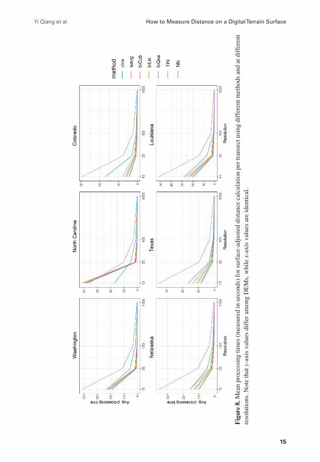
Yi Qiang et al How to Measure Distance on a Digital Terrain Surface
15
Fig
ure
8 M
ean
proc
essi
ng ti
mes
(mea
sure
d in
sec
onds
) for
sur
face
-adj
uste
d di
stan
ce c
alcu
latio
n pe
r tra
nsec
t usi
ng d
iffe
rent
met
hods
and
at d
iffe
rent
re
solu
tions
Not
e th
at y
-axi
s va
lues
dif
fer
amon
g D
EM
s w
hile
x-a
xis
valu
es a
re id
entic
al
Geographical Analysis
16
measured on 3 m resolution DEMs to evaluate their accuracies Residuals and RMSEs compared measured distances with LiDAR benchmark distances To reduce the overall computing time the distance calculation algorithm was optimized to reduce memory usage and processing time in a multi-core computer
The major findings in this study include (1) the distance measurement varies with DEM res-olutions surface adjustment methods and terrain types (2) Weighted Average is overall the most accurate surface adjustment for distance measurement with a few exceptions (3) there is a trade-off between DEM resolution and computing time The assessment results provide a foundation for distance-based spatial analyses on terrain surface (eg distance-based point pattern analysis and kriging interpolation) In a broader sense the study increases the understanding about the interplay between analytic methods scale and the geographical phenomena being studied
The assessment reveals the dependency of distance measurement on data resolution surface adjustment methods and terrain variations The results show a pattern of distance underestimation relative to the LiDAR benchmarks at finer resolutions (10 m and 30 m) that transitions to near equivalence or slight overestimation as pixel size increases The degree of underestimation varies with method of surface adjustment The weighted average method has the highest accuracy overall in most situations This finding may seem surprising given that the method utilizes a search neigh-borhood of only 8 adjacent pixels In terrain with high local relief one might expect that the polyno-mial methods would provide better results due to larger neighborhoods andor adjustment methods that could filter localized perturbations in elevation The results indicate that biquadratic (8 neigh-bors) and the bicubic (16 neighbors) methods tend to exaggerate underestimation While the bilinear neighborhood (4 pixels) produces residuals and RMSE values closer to the weighted average the kernel is rarely centered on the point being adjusted and this can over- or underemphasize nearby terrain nonuniformity Closest Centroid TIN and Nearest Neighbor employ even smaller neighbor-hoods (1 3 and up to 6 neighbors respectively) further exacerbating the problem Overestimation of surface-adjusted distance for all methods at 1000 m resolution may be associated with neigh-borhood bias as well the spatial extent of larger pixels may ignore local features at the same time as weighting more distant features (up to 4 8 or 16 kilometers away) in equal consideration The weighted average method adjustment is based on central tendency and qualified by inverse distance weighting which can offset the impacts of rough or uneven terrain in more distant pixels
The balance between improved accuracy and extra processing time is relevant from a prac-tical standpoint The DEMs tested here are probably too small to be useful for regional or conti-nental modeling as for example studies involving sea level rise earthquake damage or coastal storm events Even with high performance computing distance adjustment for larger study areas could require minutes or longer Moreover distance estimation is often the initial step and rarely the final product of spatial modeling The Closest Centroid method calculates distance based on elevation in rigid pixels which does not adjust the terrain surface using surrounding elevation values Thus the distance measurements of this method fluctuate at different resolutions due to the stair-step effect of DEM pixels As a consequence the method tends to over-estimate distance at finer resolutions due to including too many (small) pixels and to under-estimate distance at coarser resolutions due to averaging within large pixels Despite carrying the lowest processing time the accuracy of the Closest Centroid method should not be considered a good choice when trying to balance accuracy with processing times Higher processing times shown by TIN and Nearest Neighbor are coupled with reduced accuracy and no balance is achieved Polynomial adjustment by second and third order equations reflects similar results Given the second lowest processing time the weighted average method can be considered the optimal surface adjusting
Yi Qiang et al How to Measure Distance on a Digital Terrain Surface
17
method for distance calculation in most situations Adjustment using bilinear polynomial estima-tion can be considered an alternative with slightly less improvement in accuracy
The accuracy of the surface adjustment methods also varies in different terrain types The ac-curacy difference among methods is smallest in flat terrain such as Louisiana and Texas implying that for these terrain types the choice of surface adjustment for distance measurements matters less than for hilly and mountainous terrain Differences in error metrics for more mountainous or nonuniform terrains show greater variation especially at fine and intermediate resolutions mean-ing the choice of surface adjustment appears to have a greater impact on distance estimation in rougher terrain and at finer resolutions Error magnitudes begin to coalesce after 100 m resolution for all methods indicating that at some point the extra computations required for surface adjust-ment are simply not worth the potential improvement in accuracy Accuracy of surface-adjusted distance measurement is reduced in DEMs that contain a mix of terrain types with some flat and some hilly areas Future research must investigate the relationships between terrain roughness terrain uniformity and accuracy to better understand the full implication of these findings
As an additional note methods that perform best for distance calculation may or may not be optimal for other tasks such as estimating surface-adjusted elevation or area Ghandehari Buttenfield and Farmer (2019) demonstrate that linear and bilinear polynomials give slightly better accuracies for surface-adjusted estimation of point elevation on DEMs although errors for any method are quite small on the order of centimeter magnitudes for terrain measured in me-ters Their study shows however that errors for all methods increase in rough terrain This reflects earlier research by Shi and Tian (2006) and Schneider (2001) showing that errors in elevation estimation are more prominent in rough terrain Ghandehari and Buttenfield (2018) compare sur-face-adjusted methods for estimating pixel surface areas finding that while a bicubic polynomial estimation gives the highest accuracy relative to a 3 m LiDAR benchmark it carries unreason-ably high processing times They modify Jennessrsquo (2004) surface area estimation method and then apply bilinear polynomial estimation to achieve nearly equivalent accuracies to the bicubic method with processing times reduced by nearly 80 (Ghandehari 2019)
As the primary objective of the study is to evaluate and compare among surface adjustment methods the simulation program is implemented in a simple parallel model which effectively reduces the computing time to a manageable level The performance of the simulation can be further improved with finer grain parallelism architectures such as OpenMP and MPI Also the program can be further parallelized by including on-the-fly transect generation and buffer area extraction These optimization options will be explored in future experiments such as surface-ad-justed area calculation for a new variety of case studies
The title of this article raises the issue of why accurate distance measurements matters in geographical analysis There are several reasons First and as described at the beginning of the article distance metrics underlie many if not most simple and compound GIS analytic methods Second it stands to reason that inaccurate distances can propagate inaccuracies throughout the entire course of spatial modeling and confound any estimates related to terrain surfaces as for ex-ample glacial recession wetlands fragmentation freight routing or debris flow estimation Third digital terrain is one of the most frequently included data layers in spatial analyses Bolstad (2019 p 485) cites the influence of terrain characteristics on a broad set of environmental functions such as soil moisture agricultural yields sediment transport and construction costs Wilson (2012 p 107) explains the important impact of terrain ldquohellip in modulating the atmospheric geomor-phic hydrologic and ecological processes operating on or near the Earthrsquos surfacerdquo He refers to Hutchinson and Gallant (2000) in arguing that the terrain is so tightly coupled with these four
Geographical Analysis
18
families of processes that characterization of the terrain directly leads to and refines insights about the nature of the processes In a nutshell geospatial analytics cannot be accurate without accurate distance metrics And because most geographic and geomorphic processes depend partially or wholly upon the land surface on which they are situated distance measurements should be per-formed on the terrain surface ldquoas the horse runsrdquo instead of ldquoas the crow fliesrdquo
With the emergence of parallel processing and the increased availability of fine resolution terrain data surface-adjusted distance metrics are becoming an operational strategy that can improve the accuracy of many types of spatial modeling although results depend upon several factors (resolution terrain type and uniformity and surface adjustment method) Three of those factors have been examined here but this study has limitations that call for additional examina-tion and assessment The characterization of terrain uniformity must be examined more formally along with possible interaction among the factors analyzed in this article Additionally the opti-mal methods choices need to be further tested and validated by embedding the surface-adjusted distance metrics into more complex analytics For instance a hypothesis to be tested is whether surface-adjusted distance can increase the accuracy of kriging interpolation Surface adjustment also needs to be embedded in full-blown surface process models to understand them in analytic practice And finally the assessment of distance measurement shows that choosing an appropri-ate (not necessarily the finest) scale is important for spatial analysis and modeling Quattrochi and Goodchild (1997) suggest that geographical analyses should be conducted at the operational scale (also referred to by Montello (2001) as phenomenon scale) where the studied processes operate since slight changes in these processes can invoke pronounced changes in model results The results reported in this study reveal that the optimal DEM resolutions for distance mea-surement varies among different surface adjustment methods and terrain types Importantly the choice of a method may also depend upon task (measuring distance surface area or volume) As distance is the most fundamental metric for geographical analyses the knowledge generated in this study lays a foundation for developing scale-sensitive analysis tools on a terrain surface
Acknowledgment
The authors acknowledge excellent and constructive comments from reviewers which strength-ened the text
Funding information
This article is based on work supported by the US National Science under the Methodology Measurement amp Stats (MMS) Program (Award No 1853866) This article is also based on work that is part of the Data Harmonization Initiative at Earth Lab (httpswwwcolor adoeduearth lab) supported by an investment from the University of Colorado Grand Challenge Initiative Any opinions findings and conclusions or recommendations expressed in this material are those of the authors and do not necessarily reflect the views of the funding agencies
Appendix
This appendix documents the data sets and their download sources used for the experiments in the manuscript The exact specifications are included here in the interests of reproducible sci-ence so that interested readers can replicate the study using the same data sets
Yi Qiang et al How to Measure Distance on a Digital Terrain Surface
19
Benchmark LiDAR data
State Benchmark LiDAR datasets
Colorado 2010 South San Luis Lakes LidarNebraska 2009 Nebraska Department of Natural Resources (DNR) South Central
Nebraska LidarNorth Carolina 2003 North Carolina Floodplain Mapping Program (NCFMP) LidarTexas 2011 Texas Natural Resources Information System (TNRIS) Lidar Bell
Burnet and McLennan CountiesWashington 2006 USGS Lidar North Puget Sound WashingtonLouisiana 1999 Louisiana Lidar Project (1999ndash2008)
Tiles of 10 m DEMsThe following tiles are available to download in USGS TNM Download httpsviewernatio nalmapgovbasic
State Tiles of 10 m DEM
Colorado USGS NED ned19_n39x25_w106x25_co_arkansasvalley_2010 19 arc-second 2012 15 times 15 min IMGUSGS NED ned19_n39x00_w106x50_co_arkansasvalley_2010 19 arc-second 2012 15 times 15 min IMGUSGS NED ned19_n38x75_w106x00_co_arkansasvalley_2010 19 arc-second 2012 15 times 15 min IMGUSGS NED ned19_n39x50_w106x00_co_grandco_2010 19 arc-second 2011 15 times 15 min IMGUSGS NED ned19_n38x75_w106x50_co_arkansasvalley_2010 19 arc-second 2012 15 times 15 min IMGUSGS NED ned19_n38x25_w106x25_co_sanluisvalley_2011 19 arc-second 2012 15 times 15 min IMGUSGS NED ned19_n38x50_w106x00_co_arkansasvalley_2010 19 arc-second 2012 15 times 15 min IMGUSGS NED ned19_n38x25_w106x00_co_arkansasvalley_2010 19 arc-second 2012 15 times 15 min IMGUSGS NED ned19_n38x25_w106x25_co_arkansasvalley_2 010 19 arc-second 2012 15 times 15 min IMGUSGS NED ned19_n39x25_w106x50_co_arkansasvalley_2010 19 arc-second 2012 15 times 15 min IMGUSGS NED ned19_n38x25_w106x00_co_sanluisvalley_2011 19 arc-second 2012 15 times 15 min IMGUSGS NED ned19_n39x00_w106x00_co_arkansasvalley_2010 19 arc-second 2012 15 times 15 min IMGUSGS NED ned19_n39x50_w106x25_co_arkansasvalley_2010 19 arc-second 2012 15 times 15 min IMGUSGS NED ned19_n38x50_w106x25_co_arkansasvalley_2010 19 arc-second 2012 15 times 15 min IMGUSGS NED ned19_n38x25_w106x50_co_sanluisvalley_2011 19 arc-second 2012 15 times 15 min IMG
Geographical Analysis
20
State Tiles of 10 m DEM
USGS NED ned19_n39x50_w106x50_co_arkansasvalley_2010 19 arc-second 2012 15 times 15 min IMGUSGS NED ned19_n38x75_w106x25_co_arkansasvalley_2010 19 arc-second 2012 15 times 15 min IMGUSGS NED ned19_n39x00_w106x25_co_arkansasvalley_2010 19 arc-second 2012 15 times 15 min IMGUSGS NED ned19_n38x25_w105x75_co_sanluisvalley_2011 19 arc-second 2012 15 times 15 min IMGUSGS NED ned19_n39x75_w106x00_co_grandco_2010 19 arc-second 2011 15 times 15 min IMGUSGS NED ned19_n38x00_w106x25_co_sanluisvalley_2011 19 arc-second 2012 15 times 15 min IMGUSGS NED ned19_n38x00_w106x00_co_sanluisvalley_2011 19 arc-second 2012 15 times 15 min IMGUSGS NED ned19_n38x00_w106x50_co_sanluisvalley_2011 19 arc-second 2012 15 times 15 min IMGUSGS NED ned19_n38x00_w105x75_co_sanluisvalley_2011 19 arc-second 2012 15 times 15 min IMG
Nebraska USGS NED ned19_n40x50_w100x25_ne_rainwater_2009 19 arc-second 2011 15 times 15 min IMGUSGS NED ned19_n40x50_w100x00_ne_rainwater_2009 19 arc-second 2011 15 times 15 min IMGUSGS NED ned19_n40x50_w100x50_ne_rainwater_2009 19 arc-second 2011 15 times 15 min IMGUSGS NED ned19_n40x75_w100x75_ne_rainwater_2009 19 arc-second 2011 15 times 15 min IMGUSGS NED ned19_n40x75_w100x00_ne_rainwater_2009 19 arc-second 2011 15 times 15 min IMGUSGS NED ned19_n40x75_w100x25_ne_rainwater_2009 19 arc-second 2011 15 times 15 min IMGUSGS NED ned19_n40x75_w100x50_ne_rainwater_2009 19 arc-second 2011 15 times 15 min IMGUSGS NED ned19_n40x50_w100x75_ne_rainwater_2009 19 arc-second 2011 15 times 15 min IMGUSGS NED ned19_n40x75_w101x00_ne_rainwater_2009 19 arc-second 2011 15 times 15 min IMGUSGS NED ned19_n40x50_w101x00_ne_rainwater_2009 19 arc-second 2011 15 times 15 min IMGUSGS NED ned19_n40x25_w100x00_ne_rainwater_2009 19 arc-second 2011 15 times 15 min IMGUSGS NED ned19_n40x25_w100x50_ne_rainwater_2009 19 arc-second 2011 15 times 15 min IMGUSGS NED ned19_n40x25_w100x25_ne_rainwater_2009 19 arc-second 2011 15 times 15 min IMG
Yi Qiang et al How to Measure Distance on a Digital Terrain Surface
21
State Tiles of 10 m DEM
USGS NED ned19_n40x25_w100x75_ne_rainwater_2009 19 arc-second 2011 15 times 15 min IMGUSGS NED ned19_n41x00_w100x75_ne_rainwater_2009 19 arc-second 2011 15 times 15 min IMGUSGS NED ned19_n41x00_w100x00_ne_rainwater_2009 19 arc-second 2011 15 times 15 min IMGUSGS NED ned19_n41x00_w100x50_ne_rainwater_2009 19 arc-second 2011 15 times 15 min IMGUSGS NED ned19_n41x00_w100x25_ne_rainwater_2009 19 arc-second 2011 15 times 15 min IMGUSGS NED ned19_n40x75_w099x75_ne_rainwater_2009 19 arc-second 2011 15 times 15 min IMGUSGS NED ned19_n40x50_w099x75_ne_rainwater_2009 19 arc-second 2011 15 times 15 min IMGUSGS NED ned19_n40x25_w101x00_ne_rainwater_2009 19 arc-second 2011 15 times 15 min IMGUSGS NED ned19_n41x00_w101x00_ne_rainwater_2009 19 arc-second 2011 15 times 15 min IMGUSGS NED ned19_n40x25_w099x75_ne_rainwater_2009 19 arc-second 2011 15 times 15 min IMGUSGS NED ned19_n41x00_w099x75_ne_rainwater_2009 19 arc-second 2011 15 times 15 min IMG
North Carolina
USGS NED ned19_n36x00_w081x50_nc_statewide_2003 19 arc-second 2012 15 times 15 min IMGUSGS NED ned19_n36x00_w082x00_nc_statewide_2003 19 arc-second 2012 15 times 15 min IMGUSGS NED ned19_n36x00_w081x25_nc_statewide_2003 19 arc-second 2012 15 times 15 min IMGUSGS NED ned19_n36x00_w081x75_nc_statewide_2003 19 arc-second 2012 15 times 15 min IMGUSGS NED ned19_n36x00_w081x00_nc_statewide_2003 19 arc-second 2012 15 times 15 min IMGUSGS NED ned19_n36x00_w082x25_nc_statewide_2003 19 arc-second 2012 15 times 15 min IMGUSGS NED ned19_n35x75_w082x00_nc_statewide_2003 19 arc-second 2012 15 times 15 min IMGUSGS NED ned19_n35x75_w081x25_nc_statewide_2003 19 arc-second 2012 15 times 15 min IMGUSGS NED ned19_n35x75_w081x50_nc_statewide_2003 19 arc-second 2012 15 times 15 min IMGUSGS NED ned19_n35x75_w081x75_nc_statewide_2003 19 arc-second 2012 15 times 15 min IMGUSGS NED ned19_n35x75_w081x00_nc_statewide_2003 19 arc-second 2012 15 times 15 min IMG
Geographical Analysis
22
State Tiles of 10 m DEM
USGS NED ned19_n35x75_w082x25_nc_statewide_2003 19 arc-second 2012 15 times 15 min IMGUSGS NED ned19_n36x25_w081x50_nc_statewide_2003 19 arc-second 2012 15 times 15 min IMGUSGS NED ned19_n36x25_w081x00_nc_statewide_2003 19 arc-second 2012 15 times 15 min IMGUSGS NED ned19_n36x25_w081x25_nc_statewide_2003 19 arc-second 2012 15 times 15 min IMGUSGS NED ned19_n36x25_w082x00_nc_statewide_2003 19 arc-second 2012 15 times 15 min IMGUSGS NED ned19_n36x25_w081x75_nc_statewide_2003 19 arc-second 2012 15 times 15 min IMGUSGS NED ned19_n36x25_w082x25_nc_statewide_2003 19 arc-second 2012 15 times 15 min IMGUSGS NED ned19_n36x00_w080x75_nc_statewide_2003 19 arc-second 2012 15 times 15 min IMGUSGS NED ned19_n35x75_w080x75_nc_statewide_2003 19 arc-second 2012 15 times 15 min IMGUSGS NED ned19_n36x25_w080x75_nc_statewide_2003 19 arc-second 2012 15 times 15 min IMG
Texas USGS NED ned19_n31x50_w097x50_tx_bellburnetmclennancos_2011 19 arc-second 2012 15 times 15 min IMGUSGS NED ned19_n31x25_w097x25_tx_bellburnetmclennancos_2011 19 arc-second 2012 15 times 15 min IMGUSGS NED ned19_n31x00_w098x25_tx_bellburnetmclennancos_2011 19 arc-second 2012 15 times 15 min IMGUSGS NED ned19_n31x25_w097x50_tx_bellburnetmclennancos_2011 19 arc-second 2012 15 times 15 min IMGUSGS NED ned19_n31x50_w097x75_tx_bellburnetmclennancos_2011 19 arc-second 2012 15 times 15 min IMGUSGS NED ned19_n31x75_w097x25_tx_bellburnetmclennancos_2011 19 arc-second 2012 15 times 15 min IMGUSGS NED ned19_n31x25_w098x25_tx_bellburnetmclennancos_2011 19 arc-second 2012 15 times 15 min IMGUSGS NED ned19_n31x00_w098x00_tx_bellburnetmclennancos_2011 19 arc-second 2012 15 timestimes 15 min IMGUSGS NED ned19_n31x25_w097x75_tx_bellburnetmclennancos_2011 19 arc-second 2012 15 times 15 min IMGUSGS NED ned19_n31x00_w097x50_tx_bellburnetmclennancos_2011 19 arc-second 2012 15 times 15 min IMGUSGS NED ned19_n31x00_w097x75_tx_bellburnetmclennancos_2011 19 arc-second 2012 15 times 15 min IMGUSGS NED ned19_n31x75_w097x50_tx_bellburnetmclennancos_2011 19 arc-second 2012 15 times 15 min IMG
Yi Qiang et al How to Measure Distance on a Digital Terrain Surface
23
State Tiles of 10 m DEM
USGS NED ned19_n31x25_w098x00_tx_bellburnetmclennancos_2011 19 arc-second 2012 15 times 15 min IMGUSGS NED ned19_n31x00_w097x25_tx_bellburnetmclennancos_2011 19 arc-second 2012 15 times 15 min IMGUSGS NED ned19_n31x50_w097x25_tx_bellburnetmclennancos_2011 19 arc-second 2012 15 times 15 min IMGUSGS NED ned19_n30x75_w098x25_tx_bellburnetmclennancos_2011 19 arc-second 2012 15 times 15 min IMGUSGS NED ned19_n30x75_w098x00_tx_bellburnetmclennancos_2011 19 arc-second 2012 15 times 15 min IMGUSGS NED ned19_n30x75_w097x50_tx_bellburnetmclennancos_2011 19 arc-second 2012 15 times 15 min IMGUSGS NED ned19_n30x75_w098x00_tx_central_llano_2007 19 arc-second 2010 15 times 15 min IMGUSGS NED ned19_n30x75_w098x25_tx_central_llano_2007 19 arc-second 2010 15 times 15 min IMGUSGS NED ned19_n31x75_w097x00_tx_bellburnetmclennancos_2011 19 arc-second 2012 15 times 15 min IMGUSGS NED ned19_n31x50_w097x00_tx_bellburnetmclennancos_2011 19 arc-second 2012 15 times 15 min IMGUSGS NED ned19_n31x25_w098x50_tx_central_llano_2007 19 arc-second 2010 15 times 15 min IMGUSGS NED ned19_n31x50_w098x50_tx_central_llano_2007 19 arc-second 2010 15 times 15 min IMGUSGS NED ned19_n31x00_w098x50_tx_central_llano_2007 19 arc-second 2010 15 times 15 min IMGUSGS NED ned19_n31x75_w098x50_tx_central_llano_2007 19 arc-second 2010 15 times 15 min IMGUSGS NED ned19_n31x00_w098x50_tx_bellburnetmclennancos_2011 19 arc-second 2012 15 times 15 min IMGUSGS NED ned19_n30x75_w098x50_tx_central_llano_2007 19 arc-second 2010 15 times 15 min IMGUSGS NED ned19_n30x75_w098x50_tx_bellburnetmclennancos_2011 19 arc-second 2012 15 times 15 min IMG
Washington USGS NED ned19_n48x50_w122x00_wa_northpugetsound_2006 19 arc-second 2009 15 times 15 min IMGUSGS NED ned19_n48x50_w122x50_wa_puget_sound_2000 19 arc-second 2012 15 times 15 min IMGUSGS NED ned19_n48x50_w121x50_wa_northpugetsound_2006 19 arc-second 2009 15 times 15 min IMGUSGS NED ned19_n49x00_w122x50_wa_northpugetsound_2006 19 arc-second 2009 15 times 15 min IMGUSGS NED ned19_n48x75_w122x75_wa_sanjuanco_2009 19 arc-second 2011 15 times 15 min IMG
Geographical Analysis
24
State Tiles of 10 m DEM
USGS NED ned19_n48x50_w122x25_wa_northpugetsound_2006 19 arc-second 2009 15 times 15 min IMGUSGS NED ned19_n48x75_w121x25_wa_northpugetsound_2006 19 arc-second 2009 15 times 15 min IMGUSGS NED ned19_n49x00_w121x25_wa_northpugetsound_2006 19 arc-second 2009 15 times 15 min IMGUSGS NED ned19_n49x00_w122x00_wa_northpugetsound_2006 19 arc-second 2009 15 times 15 min IMGUSGS NED ned19_n48x50_w122x75_wa_puget_sound_2000 19 arc-second 2012 15 times 15 min IMGUSGS NED ned19_n48x75_w122x00_wa_northpugetsound_2006 19 arc-second 2009 15 times 15 min IMGUSGS NED ned19_n48x75_w122x75_wa_northpugetsound_2006 19 arc-second 2009 15 times 15 min IMGUSGS NED ned19_n48x75_w121x75_wa_northpugetsound_2006 19 arc-second 2009 15 times 15 min IMGUSGS NED ned19_n48x75_w122x25_wa_northpugetsound_2006 19 arc-second 2009 15 times 15 min IMGUSGS NED ned19_n49x00_w121x75_wa_northpugetsound_2006 19 arc-second 2009 15 times 15 min IMGUSGS NED ned19_n48x75_w122x50_wa_northpugetsound_2006 19 arc-second 2009 15 times 15 min IMGUSGS NED ned19_n49x00_w122x25_wa_northpugetsound_2006 19 arc-second 2009 15 times 15 min IMGUSGS NED ned19_n48x50_w122x50_wa_northpugetsound_2006 19 arc-second 2009 15 times 15 min IMGUSGS NED ned19_n48x50_w122x75_wa_northpugetsound_2006 19 arc-second 2009 15 times 15 min IMGUSGS NED ned19_n48x75_w121x50_wa_northpugetsound_2006 19 arc-second 2009 15 times 15 min IMGUSGS NED ned19_n49x00_w122x75_wa_northpugetsound_2006 19 arc-second 2009 15 times 15 min IMGUSGS NED ned19_n48x50_w121x75_wa_northpugetsound_2006 19 arc-second 2009 15 times 15 min IMGUSGS NED ned19_n49x25_w122x25_wa_northpugetsound_2006 19 arc-second 2009 15 times 15 min IMGUSGS NED ned19_n49x25_w122x50_wa_northpugetsound_2006 19 arc-second 2009 15 times 15 min IMGUSGS NED ned19_n49x25_w122x00_wa_northpugetsound_2006 19 arc-second 2009 15 times 15 min IMGUSGS NED ned19_n49x25_w122x75_wa_northpugetsound_2006 19 arc-second 2009 15 times 15 min IMGUSGS NED ned19_n48x25_w122x50_wa_puget_sound_2000 19 arc-second 2012 15 times 15 min IMG
Yi Qiang et al How to Measure Distance on a Digital Terrain Surface
25
State Tiles of 10 m DEM
USGS NED ned19_n48x25_w122x75_wa_puget_sound_2000 19 arc-second 2012 15 times 15 min IMGUSGS NED ned19_n48x50_w123x00_wa_puget_sound_2000 19 arc-second 2012 15 times 15 min IMGUSGS NED ned19_n48x75_w123x00_wa_sanjuanco_2009 19 arc-second 2011 15 times 15 min IMGUSGS NED ned19_n49x00_w123x00_wa_northpugetsound_2006 19 arc-second 2009 15 times 15 min IMGUSGS NED ned19_n48x50_w123x00_wa_sanjuanco_2009 19 arc-second 2011 15 times 15 min IMGUSGS NED ned19_n49x25_w123x00_wa_northpugetsound_2006 19 arc-second 2009 15 times 15 min IMGUSGS NED ned19_n48x25_w123x00_wa_puget_sound_2000 19 arc-second 2012 15 times 15 min IMG
Louisiana USGS NED ned19_n30x75_w091x50_la_statewide_2006 19 arc-second 2009 15 times 15 min IMGUSGS NED ned19_n30x50_w091x00_la_statewide_2006 19 arc-second 2009 15 times 15 min IMGUSGS NED ned19_n30x50_w091x50_la_atchafalayabasin_2010 19 arc-second 2011 15 times 15 min IMGUSGS NED ned19_n30x50_w091x50_la_statewide_2006 19 arc-second 2009 15 times 15 min IMGUSGS NED ned19_n30x75_w091x00_la_statewide_2006 19 arc-second 2009 15 times 15 min IMGUSGS NED ned19_n30x75_w091x25_la_statewide_2006 19 arc-second 2009 15 times 15 min IMGUSGS NED ned19_n30x75_w090x75_la_statewide_2006 19 arc-second 2009 15 times 15 min IMGUSGS NED ned19_n30x50_w091x25_la_statewide_2006 19 arc-second 2009 15 times 15 min IMGUSGS NED ned19_n30x50_w090x75_la_statewide_2006 19 arc-second 2009 15 times 15 min IMGUSGS NED ned19_n30x50_w091x50_LA-USGS_Atchafalaya2_2012_2014 19 arc-second 20140615 15 15 min IMGUSGS NED ned19_n31x00_w091x50_la_statewide_2006 19 arc-second 2009 15 times 15 min IMGUSGS NED ned19_n31x00_w091x25_la_statewide_2006 19 arc-second 2009 15 times 15 min IMGUSGS NED ned19_n31x00_w091x00_la_statewide_2006 19 arc-second 2009 15 times 15 min IMGUSGS NED ned19_n31x00_w090x75_la_statewide_2006 19 arc-second 2009 15 times 15 min IMGUSGS NED ned19_n30x25_w091x00_la_statewide_2006 19 arc-second 2009 15 times 15 min IMG
Geographical Analysis
26
State Tiles of 10 m DEM
USGS NED ned19_n30x25_w091x50_la_atchafalayabasin_2010 19 arc-second 2011 15 times 15 min IMGUSGS NED ned19_n30x25_w091x50_la_statewide_2006 19 arc-second 2009 15 times 15 min IMGUSGS NED ned19_n30x25_w090x75_la_statewide_2006 19 arc-second 2009 15 times 15 min IMGUSGS NED ned19_n30x25_w091x25_la_statewide_2006 19 arc-second 2009 15 times 15 min IMGUSGS NED ned19_n30x25_w091x50_LA-USGS_Atchafalaya2_2012_2014 19 arc-second 20140615 15 times 15 min IMGUSGS NED ned19_n30x25_w091x25_LA-USGS_Atchafalaya2_2012_2014 19 arc-second 20140615 15 times 15 min IMGUSGS NED ned19_n30x75_w090x50_la_statewide_2006 19 arc-second 2009 15 times 15 min IMGUSGS NED ned19_n30x50_w090x50_la_statewide_2006 19 arc-second 2009 15 times 15 min IMGUSGS NED ned19_n30x75_w091x75_la_statewide_2006 19 arc-second 2009 15 times 15 min IMGUSGS NED ned19_n30x50_w091x75_la_atchafalayabasin_2010 19 arc-second 2011 15 times 15 min IMGUSGS NED ned19_n30x50_w091x75_la_statewide_2006 19 arc-second 2009 15 times 15 min IMGUSGS NED ned19_n30x75_w091x75_la_atchafalayabasin_2010 19 arc-second 2011 15 times 15 min IMGUSGS NED ned19_n30x75_w091x75_LA-USGS_Atchafalaya2_2012_2014 19 arc-second 20140615 15 times 15 min IMGUSGS NED ned19_n30x50_w091x75_LA-USGS_Atchafalaya2_2012_2014 19 arc-second 20140615 15 times 15 min IMGUSGS NED ned19_n31x00_w090x50_la_statewide_2006 19 arc-second 2009 15 times 15 min IMGUSGS NED ned19_n30x25_w090x50_la_statewide_2006 19 arc-second 2009 15 times 15 min IMGUSGS NED ned19_n31x00_w091x75_la_statewide_2006 19 arc-second 2009 15 times 15 min IMGUSGS NED ned19_n31x00_w091x75_LA-USGS_Atchafalaya2_2012_2014 19 arc-second 20140615 15 times 15 min IMGUSGS NED ned19_n30x25_w091x75_la_atchafalayabasin_2010 19 arc-second 2011 15 times 15 min IMGUSGS NED ned19_n30x25_w091x75_la_statewide_2006 19 arc-second 2009 15 times 15 min IMGUSGS NED ned19_n30x25_w091x75_LA-USGS_Atchafalaya2_2012_2014 19 arc-second 20140615 15 times 15 min IMG
Tiles of 30 m DEMs
Yi Qiang et al How to Measure Distance on a Digital Terrain Surface
27
The following tiles are available to download in USGS TNM Download httpsviewernatio nalmapgovbasic
State Tiles of 30 m DEM
Colorado USGS NED 13 arc-second n40w107USGS NED n39w107 13 arc-secondUSGS NED 13 arc-second n40w106USGS NED 13 arc-second n39w106
Nebraska USGS NED 13 arc-second n41w101 1 x 1 degree ArcGrid 2019USGS NED 13 arc-second n41w100 1 x 1 degree ArcGrid 2019
North Carolina USGS NED 13 arc-second n36w082 1 x 1 degree ArcGrid 2019USGS NED n36w081 13 arc-second 2013 1 x 1 degree ArcGridUSGS NED 13 arc-second n36w083 1 x 1 degree ArcGrid 2017USGS NED 13 arc-second n37w082 1 x 1 degree ArcGrid 2019USGS NED 13 arc-second n37w081 1 x 1 degree ArcGrid 2018USGS NED 13 arc-second n37w083 1 x 1 degree ArcGrid 2018
Texas USGS NED 13 arc-second n32w098 1 x 1 degree ArcGrid 2019USGS NED 13 arc-second n31w098 1 x 1 degree ArcGrid 2019USGS NED 13 arc-second n32w099 1 x 1 degree ArcGrid 2019USGS NED 13 arc-second n31w099 1 x 1 degree ArcGrid 2019USGS NED 13 arc-second n32w097 1 x 1 degree ArcGrid 2019USGS NED 13 arc-second n31w097 1 x 1 degree ArcGrid 2019
Washington USGS NED 13 arc-second n49w122 1 x 1 degree ArcGrid 2018USGS NED 13 arc-second n49w123 1 x 1 degree ArcGrid 2019USGS NED 13 arc-second n50w122 1 x 1 degree ArcGrid 2018USGS NED 13 arc-second n49w121 1 x 1 degree ArcGrid 2018USGS NED 13 arc-second n50w123 1 x 1 degree ArcGrid 2018
Louisiana USGS NED 13 arc-second n31w091 1 x 1 degree ArcGrid 2019USGS NED 13 arc-second n31w092 1 x 1 degree ArcGrid 2019
Tiles of 100 m and 1000 m DEMsThe following tiles are available to download in USGSrsquos website httpsddscrusgsgovsrtmversi on2_1
States Tiles 100 m DEM Tiles 1000 m DEM
Colorado N38W107SRTMGL3 w140n40SRTM30N39W107SRTMGL3N39W106SRTMGL3N38W106SRTMGL3
Nebraska N40W100SRTMGL3 w140n90SRTM30N40W101SRTMGL3
North Carolina N35W082SRTMGL3 w140n90SRTM30N35W081SRTMGL3N35W083SRTMGL3
Texas N29W098SRTMGL3N29W099SRTMGL3
Washington N48W123SRTMGL3 w100n40SRTM30N48W122SRTMGL3
Louisiana N29W091SRTMGL3 w100n40SRTM30N29W092SRTMGL3
Geographical Analysis
28
Tab
les
of
the
anal
ysis
res
ult
s
Tab
le A
1 R
esid
ual
Ave
rage
Res
idua
l R
MSE
and
Pro
cess
ing
Tim
e fo
r W
ashi
ngto
n I
nter
pola
tion
Met
hods
Inc
lude
(in
Top
-to-
Bot
tom
Ord
er)
Bic
ubic
Bili
near
and
Biq
uadr
atic
pol
ynom
ials
Clo
sest
Cen
troi
d N
eare
st N
eigh
bor
Tri
angu
late
d Ir
regu
lar
Net
wor
k a
nd W
eigh
ted
Ave
rage
Res
olut
ion
Stud
y ar
eaIn
terp
olat
ion
met
hod
Avg
res
idua
l (m
)A
vg t
ime
(s)
Avg
rat
io o
f re
sidu
alR
MSE
(m
)
10W
ashi
ngto
nbi
Cub
minus474
29
231
60minus0
016
0859
825
10W
ashi
ngto
nbi
Lin
minus275
87
210
59minus0
009
4235
463
10W
ashi
ngto
nbi
Qua
minus350
39
216
51minus0
011
9144
494
10W
ashi
ngto
ncl
os1
317
0319
142
004
514
166
534
10W
ashi
ngto
nN
Nminus8
785
922
620
minus00
2975
110
814
10W
ashi
ngto
nT
INminus7
763
841
305
minus00
2623
975
0410
Was
hing
ton
wav
g37
99
196
900
0013
599
64
30W
ashi
ngto
nbi
Cub
minus319
35
200
4minus0
010
8939
954
30W
ashi
ngto
nbi
Lin
minus136
67
117
3minus0
004
7117
310
30W
ashi
ngto
nbi
Qua
minus210
48
143
0minus0
007
1726
271
30W
ashi
ngto
ncl
os1
069
140
817
003
723
137
121
30W
ashi
ngto
nN
Nminus5
671
85
546
minus00
1943
722
4030
Was
hing
ton
TIN
minus476
51
113
48minus0
016
1159
879
30W
ashi
ngto
nw
avg
745
10
865
000
269
130
6510
0W
ashi
ngto
nbi
Cub
minus306
76
050
3minus0
010
5040
213
100
Was
hing
ton
biL
inminus1
754
80
273
minus00
0599
237
1110
0W
ashi
ngto
nbi
Qua
minus217
31
034
0minus0
007
2829
031
100
Was
hing
ton
clos
698
930
204
002
469
915
6410
0W
ashi
ngto
nN
Nminus4
112
01
650
minus00
1399
532
3210
0W
ashi
ngto
nT
INminus3
183
73
383
minus00
1065
416
4110
0W
ashi
ngto
nw
avg
minus22
260
201
minus00
0032
111
771
000
Was
hing
ton
biC
ubminus2
395
00
108
minus00
0719
548
591
000
Was
hing
ton
biL
inminus2
007
10
077
minus00
0754
516
001
000
Was
hing
ton
biQ
uaminus2
225
70
083
minus00
0850
543
431
000
Was
hing
ton
clos
299
990
068
001
204
578
811
000
Was
hing
ton
NN
minus223
18
014
7minus0
007
6052
918
100
0W
ashi
ngto
nT
INminus1
614
80
450
minus00
0758
471
211
000
Was
hing
ton
wav
gminus1
298
90
068
minus00
0484
496
20
Yi Qiang et al How to Measure Distance on a Digital Terrain Surface
29
Table A2 Residual Average Residual RMSE and Processing Time for North Carolina Interpolation Methods Include (in Top-to-Bottom Order) Bicubic Bilinear and Biquadratic polynomials Closest Centroid Nearest Neighbor Triangulated Irregular Network and Weighted Average
Resolution Study Area MethodAvg residual Avg time
Avg ratio of residual RMSE
10 North Carolina biCub minus39280 82186 minus000973 4971710 North Carolina biLin minus25592 78635 minus000643 3262710 North Carolina biQua minus30551 79250 minus000761 3872610 North Carolina clos 103191 75460 002535 13173110 North Carolina NN minus79594 34227 minus001958 10150610 North Carolina TIN minus75426 72281 minus001853 9519210 North Carolina wavg minus886 76333 minus000033 715030 North Carolina biCub minus36234 4078 minus000897 4675230 North Carolina biLin minus18032 2678 minus000452 2319130 North Carolina biQua minus25272 3131 minus000626 3251230 North Carolina clos 79456 1949 001972 10139030 North Carolina NN minus54725 10186 minus001360 7172030 North Carolina TIN minus52388 20687 minus001293 6667230 North Carolina wavg minus3793 2088 minus000093 6429100 North Carolina biCub minus38245 0921 minus000938 50519100 North Carolina biLin minus30836 0499 minus000754 40788100 North Carolina biQua minus33905 0624 minus000835 44764100 North Carolina clos 9981 0357 000278 19506100 North Carolina NN minus41975 2560 minus001046 55973100 North Carolina TIN minus39808 5935 minus000986 52072100 North Carolina wavg minus25205 0364 minus000618 330921000 North Carolina biCub minus13916 0122 minus000105 641361000 North Carolina biLin minus10973 0091 minus000167 623531000 North Carolina biQua minus14067 0096 minus000124 643461000 North Carolina clos minus5074 0083 minus000054 610341000 North Carolina NN minus14628 0120 minus000200 639841000 North Carolina TIN minus12287 0468 minus000255 623091000 North Carolina wavg minus13194 0081 minus000080 63061
Geographical Analysis
30
Table A3 Residual Average Residual RMSE and Processing Time for Colorado Interpolation Methods Include (in Top-to-Bottom Order) Bicubic Bilinear and Biquadratic Polynomials Closest Centroid Nearest Neighbor Triangulated Irregular Network and Weighted Average
Resolution Study Area Method Avg residual Avg timeAvg ratio of residual RMSE
10 Colorado biCub minus21068 7957 minus000968 2870810 Colorado biLin minus11997 5588 minus000566 1680410 Colorado biQua minus15591 6381 minus000729 2153010 Colorado clos 60424 4200 002749 7803210 Colorado NN minus35698 17031 minus001629 5060910 Colorado TIN minus42632 29384 minus001930 5665410 Colorado wavg 1410 4499 000046 585530 Colorado biCub minus18084 1800 minus000808 2462830 Colorado biLin minus8422 1095 minus000382 1198230 Colorado biQua minus12450 1309 minus000560 1721130 Colorado clos 45183 0729 002082 5887330 Colorado NN minus26450 3091 minus001182 3729630 Colorado TIN minus29240 7784 minus001326 3921530 Colorado wavg minus513 0798 minus000020 5506100 Colorado biCub minus18886 0520 minus000839 25817100 Colorado biLin minus13441 0311 minus000593 18908100 Colorado biQua minus15535 0367 minus000703 21444100 Colorado clos 16414 0208 000757 24211100 Colorado NN minus19998 0736 minus000922 28223100 Colorado TIN minus21186 2349 minus000992 28612100 Colorado wavg minus9335 0226 minus000413 143081000 Colorado biCub minus9685 0077 minus000350 630701000 Colorado biLin minus6277 0059 000636 633641000 Colorado biQua minus6457 0061 000222 586041000 Colorado clos minus911 0054 000077 597911000 Colorado NN minus9166 0078 000324 599841000 Colorado TIN minus8685 0234 minus000152 590841000 Colorado wavg minus3811 0054 000378 57750
Yi Qiang et al How to Measure Distance on a Digital Terrain Surface
31
Table A4 Residual Average Residual RMSE and Processing Time for Nebraska Interpolation Methods Include (in Top-to-Bottom Order) Bicubic Bilinear and Biquadratic polynomials Closest Centroid Nearest Neighbor Triangulated Irregular Network and Weighted Average
Resolution Study Area Method Avg residual Avg timeAvg ratio of residual RMSE
10 Nebraska biCub minus15507 15751 minus000438 1842310 Nebraska biLin minus8786 12139 minus000249 1051610 Nebraska biQua minus11645 13238 minus000329 1385010 Nebraska clos 36339 9779 001024 4281710 Nebraska NN minus24660 15574 minus000693 2919010 Nebraska TIN minus24193 35472 minus000681 2859210 Nebraska wavg minus1845 10406 minus000054 285030 Nebraska biCub minus12290 2861 minus000345 1480730 Nebraska biLin minus6632 1831 minus000187 812330 Nebraska biQua minus9544 2162 minus000269 1150730 Nebraska clos 23939 1287 000676 2831630 Nebraska NN minus15898 4681 minus000447 1896130 Nebraska TIN minus15391 10863 minus000436 1831230 Nebraska wavg minus3888 1374 minus000111 5014100 Nebraska biCub minus9337 0776 minus000268 12040100 Nebraska biLin minus7733 0470 minus000222 10434100 Nebraska biQua minus8326 0560 minus000232 11135100 Nebraska clos 1640 0330 000043 5837100 Nebraska NN minus10137 1126 minus000282 13097100 Nebraska TIN minus9717 3289 minus000271 12620100 Nebraska wavg minus6860 0341 minus000198 97011000 Nebraska biCub minus599 0131 000065 443391000 Nebraska biLin minus846 0090 000058 457281000 Nebraska biQua minus715 0098 000009 426081000 Nebraska clos 070 0076 minus000046 439671000 Nebraska NN minus2165 0120 minus000030 448871000 Nebraska TIN 049 0437 000077 452231000 Nebraska wavg minus658 0077 minus000055 44366
Geographical Analysis
32
Table A5 Residual Average Residual RMSE and Processing Time for Texas Interpolation Methods Include (in Top-to-Bottom Order) Bicubic Bilinear and Biquadratic Polynomials Closest Centroid Nearest Neighbor Triangulated Irregular Network and Weighted Average
Resolution Study Area Method Avg residual Avg timeAvg ratio of residual RMSE
10 Texas biCub minus6678 13527 minus000195 814210 Texas biLin minus4630 10210 minus000135 567810 Texas biQua minus5603 11303 minus000164 682910 Texas clos 10990 8228 000317 1408710 Texas NN minus9274 16384 minus000269 1155410 Texas TIN minus9619 34548 minus000280 1183410 Texas wavg minus2283 8734 minus000067 291030 Texas biCub minus4288 2730 minus000129 552930 Texas biLin minus2693 1761 minus000087 364330 Texas biQua minus3388 2076 minus000098 444730 Texas clos 7699 1241 000218 1039430 Texas NN minus5702 3433 minus000171 735530 Texas TIN minus5518 9743 minus000169 704430 Texas wavg minus1467 1330 minus000047 2510100 Texas biCub minus3155 0775 minus000107 6498100 Texas biLin minus2425 0481 minus000080 6196100 Texas biQua minus2945 0565 minus000079 6493100 Texas clos 4061 0338 000099 7431100 Texas NN minus3677 0815 minus000113 7056100 Texas TIN minus3622 3066 minus000121 7066100 Texas wavg minus1931 0355 minus000081 59641000 Texas biCub 929 0106 000991 601131000 Texas biLin 195 0078 001138 613451000 Texas biQua 870 0082 001353 622861000 Texas clos 220 0069 000922 616651000 Texas NN 2542 0097 000987 610911000 Texas TIN minus1579 0339 000748 633421000 Texas wavg minus218 0069 000829 61030
Yi Qiang et al How to Measure Distance on a Digital Terrain Surface
33
Table A6 Residual Average Residual RMSE and Processing Time for Louisiana Interpolation Methods Include (in top-to-bottom order) Bicubic Bilinear and Biquadratic polynomials Closest Centroid Nearest Neighbor Triangulated Irregular Network and Weighted Average
Resolution Study Area Method Avg residual Avg timeAvg ratio of residual RMSE
10 Louisiana biCub minus3132 25881 minus000084 384410 Louisiana biLin minus2262 22476 minus000061 279310 Louisiana biQua minus2722 23573 minus000073 334310 Louisiana clos 2551 19252 000070 318010 Louisiana NN minus3294 27879 minus000088 402610 Louisiana TIN minus3380 51336 minus000091 411510 Louisiana wavg minus1800 20357 minus000048 222330 Louisiana biCub minus1636 2924 minus000048 257630 Louisiana biLin minus1284 1806 minus000036 220030 Louisiana biQua minus1501 2171 minus000042 248230 Louisiana clos 486 1288 000013 175630 Louisiana NN minus1645 7183 minus000045 258830 Louisiana TIN minus1642 14367 minus000046 256330 Louisiana wavg minus1154 1367 minus000030 2129100 Louisiana biCub minus706 0792 minus000014 5329100 Louisiana biLin minus818 0492 minus000019 5458100 Louisiana biQua minus532 0579 minus000017 5348100 Louisiana clos minus543 0330 minus000003 5361100 Louisiana NN minus789 0772 minus000020 5375100 Louisiana TIN minus916 3179 minus000025 5644100 Louisiana wavg minus640 0361 minus000009 55851000 Louisiana biCub 494 0109 000265 584241000 Louisiana biLin 1730 0079 000215 593021000 Louisiana biQua 839 0084 000325 613951000 Louisiana clos 744 0067 000203 603861000 Louisiana NN minus119 0112 000123 602791000 Louisiana TIN 1416 0369 000168 599011000 Louisiana wavg 1211 0070 000236 59514
Geographical Analysis
34
References
Bolstad P (2019) GIS Fundamentals A First Text on Geographic Information systems 6th ed Ann Arbor MI XanEdu Publishing Inc
Buttenfield B M Ghandehari S Leyk L Stanislawski M Brantley Y Qiang (2016) Measuring Distance ldquoAs the Horse Runsrdquo Cross-Scale Comparison of Terrain-Based Metrics International Conference on GIScience Short Paper Proceedings 1 httpdxdoiorg1021433 b3118 rh987cz
Chang K and B Tsai (1991) ldquoThe Effect of DEM Resolution on Slope and Aspect Mappingrdquo Cartography and Geographic Information Systems 18(1) 69ndash77 httpsdoiorg10155915230 40917 83805626
GDALOGR contributors (2020) GDALOGR GEOSPATIAL Data Abstraction Software Library Open Source Geospatial Foundation httpsgdalorg
Gesch D B (2007) ldquoThe National Elevation Datasetrdquo In Digital Elevation Model Technologies and Applications The DEM Users Manual 2nd ed 99ndash118
Gesch DB M J Oimoen and G A Evans (2014) ldquoAccuracy Assessment of the US Geological Survey National Elevation Dataset and Comparison with Other Large-Area Elevation Datasets SRTM and ASTERrdquo Report No 2014ndash1008 Open-File Report p 18 USGS Publications Warehouse httpsdoiorg103133ofr20 141008
Ghandehari M (2019) Cross-Scale Analysis of Surface-Adjusted Measurements in digital Elevation Models Doctoral dissertation University of Colorado Boulder
Ghandehari M and B Buttenfield (2018) ldquoSlope-Adjusted Surface Area Computations in Digital Terrainrdquo Proceedings of 5th International Conference of the International Society of Geomorphometry (Geomorphometry 2018)
Ghandehari M B P Buttenfield C J Q Farmer (2019) Comparing the accuracy of estimated terrain elevations across spatial resolution International Journal of Remote Sensing 40(13) 5025ndash5049 httpdxdoiorg10108001431 16120191577581
Gutieacuterrez M (2012) ldquoChapter 153 Applied Geomorphology in Periglacial Reginsrdquo In Geomorphology 601ndash13 Boca Raton FL Taylor amp Francis
Harms T K E A Wentz and N B Grimm (2009) ldquoSpatial Heterogeneity of Denitrification in Semi-Arid Floodplainsrdquo Ecosystems 12(1) 129ndash43 httpsdoiorg101007s1002 1-008-9212-6
Hutchinson M F and J C Gallant (2000) Digital Elevation Models and Representation of Terrain Shape httpspubli catio nscsiroaurprpublist=BROamppid=proci te46f1d e5d-172e-4f8e-8696-da3b6 f7b03ca
Jenness J S (2004) ldquoCalculating Landscape Surface Area from Digital Elevation Modelsrdquo Wildlife Society Bulletin 32(3) 829ndash39 httpsdoiorg1021930091-7648(2004)032[0829CLSAF D]20CO2
Kienzle S (2004) ldquoThe Effect of DEM Raster Resolution on First Order Second Order and Compound Terrain Derivativesrdquo Transactions in GIS 8(1) 83ndash111 httpsdoiorg101111j1467-9671200400169x
Kiessling F P Nefzger J Nolasco and U Kaintzyk (2014) Overhead Power Lines Planning Design Construction Berlin Germany Springer
Montello D R (2001) ldquoScale in Geographyrdquo In International Encyclopedia of the Social and Behavioral Sciences 13501ndash4 edited by N J Smelser and B Baltes
Oliphant T E (2006) A guide to NumPy (Vol 1) Trelgol Publishing USAQiang Y B P Buttenfield N Lam and N V de Weghe (2018) ldquoNovel Models for Multi-Scale Spatial
and Temporal Analysesrdquo In 10th International Conference on Geographic Information Science (GIScience 2018) Vol 114 551ndash557 edited by S Winter A Griffin amp M Sester Dagstuhl Germany Schloss DagstuhlndashLeibniz-Zentrum fuer Informatik httpsdoiorg104230LIPIcsGISCI ENCE201855
Qiang Y and N Van de Weghe (2019) ldquoRe-Arranging Space Time and Scales in GIS Alternative Models for Multi-Scale Spatio-Temporal Modeling and Analysesrdquo ISPRS International Journal of Geo-Information 8(2) 72 httpsdoiorg103390ijgi8 020072
Quattrochi D A and M F Goodchild (1997) Scale in Remote Sensing and GIS Boca Raton FL CRC Press
Schneider B (2001) On the Uncertainty of Local Shape of Lines and Surfaces Cartography and Geographic Information Science 28(4) 237ndash247 httpsdoiorg10155915230 40017 82152991
Yi Qiang et al How to Measure Distance on a Digital Terrain Surface
35
Shafique M M van der Meijde N Kerle and F van der Meer (2011) ldquoImpact of DEM Source and Resolution on Topographic Seismic Amplificationrdquo International Journal of Applied Earth Observation and Geoinformation 13(3) 420ndash7 httpsdoiorg101016jjag201009005
Shi W Z and Y Tian (2006) ldquoA Hybrid Interpolation Method for the Refinement of a Regular Grid Digital Elevation Modelrdquo International Journal of Geographical Information Science 20(1) 53ndash67 httpsdoiorg10108013658 81050 0286943
Sibson R (1981) ldquoA Brief Description of Natural Neighbor Interpolationrdquo In Interpolating Multivariate Data 21ndash36 New York John Wiley amp Sons
Stanislawski L V J Falgout and B P Buttenfield (2015) ldquoAutomated Extraction of Natural Drainage Density Patterns for the Conterminous United States through High-Performance Computingrdquo The Cartographic Journal 52(2) 185ndash92 httpsdoiorg10108000087 04120151119466
Stoker J M (2018) The US Geological Survey Physical Scientist The Chief Elevation Scientist for the National Geospatial Program personal communication (jstokerusgsgov) [Personal communication]
The IPython Development Team (2018) Using IPython for parallel computing httpsipypa rallelreadt hedocsioenlates t
Tucker G E and G R Hancock (2010) ldquoModelling Landscape Evolutionrdquo Earth Surface Processes and Landforms 35(1) 28ndash50 httpsdoiorg101002esp1952
University Corporation for Atmospheric Research (UCAR) (2004) Natgrid Introduction httpwwwncargucaredungmat hnatgr idnnhomehtml
Usery E L M P Finn D J Scheidt S Ruhl T Beard and M Bearden (2004) ldquoGeospatial Data Resampling and Resolution Effects on Watershed Modeling A Case Study Using the Agricultural Non-Point Source Pollution Modelrdquo Journal of Geographical Systems 6(3) 289ndash306 httpsdoiorg101007s1010 9-004-0138-z
Wilson J P (2012) ldquoDigital Terrain Modelingrdquo Geomorphology 137(1) 107ndash21 httpsdoiorg101016jgeomo rph201103012
Zhang W and D R Montgomery (1994) ldquoDigital Elevation Model Grid Size Landscape Representation and Hydrologic Simulationsrdquo Water Resources Research 30(4) 1019ndash28 httpsdoiorg10102993WR0 3553

Geographical Analysis
16
measured on 3 m resolution DEMs to evaluate their accuracies Residuals and RMSEs compared measured distances with LiDAR benchmark distances To reduce the overall computing time the distance calculation algorithm was optimized to reduce memory usage and processing time in a multi-core computer
The major findings in this study include (1) the distance measurement varies with DEM res-olutions surface adjustment methods and terrain types (2) Weighted Average is overall the most accurate surface adjustment for distance measurement with a few exceptions (3) there is a trade-off between DEM resolution and computing time The assessment results provide a foundation for distance-based spatial analyses on terrain surface (eg distance-based point pattern analysis and kriging interpolation) In a broader sense the study increases the understanding about the interplay between analytic methods scale and the geographical phenomena being studied
The assessment reveals the dependency of distance measurement on data resolution surface adjustment methods and terrain variations The results show a pattern of distance underestimation relative to the LiDAR benchmarks at finer resolutions (10 m and 30 m) that transitions to near equivalence or slight overestimation as pixel size increases The degree of underestimation varies with method of surface adjustment The weighted average method has the highest accuracy overall in most situations This finding may seem surprising given that the method utilizes a search neigh-borhood of only 8 adjacent pixels In terrain with high local relief one might expect that the polyno-mial methods would provide better results due to larger neighborhoods andor adjustment methods that could filter localized perturbations in elevation The results indicate that biquadratic (8 neigh-bors) and the bicubic (16 neighbors) methods tend to exaggerate underestimation While the bilinear neighborhood (4 pixels) produces residuals and RMSE values closer to the weighted average the kernel is rarely centered on the point being adjusted and this can over- or underemphasize nearby terrain nonuniformity Closest Centroid TIN and Nearest Neighbor employ even smaller neighbor-hoods (1 3 and up to 6 neighbors respectively) further exacerbating the problem Overestimation of surface-adjusted distance for all methods at 1000 m resolution may be associated with neigh-borhood bias as well the spatial extent of larger pixels may ignore local features at the same time as weighting more distant features (up to 4 8 or 16 kilometers away) in equal consideration The weighted average method adjustment is based on central tendency and qualified by inverse distance weighting which can offset the impacts of rough or uneven terrain in more distant pixels
The balance between improved accuracy and extra processing time is relevant from a prac-tical standpoint The DEMs tested here are probably too small to be useful for regional or conti-nental modeling as for example studies involving sea level rise earthquake damage or coastal storm events Even with high performance computing distance adjustment for larger study areas could require minutes or longer Moreover distance estimation is often the initial step and rarely the final product of spatial modeling The Closest Centroid method calculates distance based on elevation in rigid pixels which does not adjust the terrain surface using surrounding elevation values Thus the distance measurements of this method fluctuate at different resolutions due to the stair-step effect of DEM pixels As a consequence the method tends to over-estimate distance at finer resolutions due to including too many (small) pixels and to under-estimate distance at coarser resolutions due to averaging within large pixels Despite carrying the lowest processing time the accuracy of the Closest Centroid method should not be considered a good choice when trying to balance accuracy with processing times Higher processing times shown by TIN and Nearest Neighbor are coupled with reduced accuracy and no balance is achieved Polynomial adjustment by second and third order equations reflects similar results Given the second lowest processing time the weighted average method can be considered the optimal surface adjusting
Yi Qiang et al How to Measure Distance on a Digital Terrain Surface
17
method for distance calculation in most situations Adjustment using bilinear polynomial estima-tion can be considered an alternative with slightly less improvement in accuracy
The accuracy of the surface adjustment methods also varies in different terrain types The ac-curacy difference among methods is smallest in flat terrain such as Louisiana and Texas implying that for these terrain types the choice of surface adjustment for distance measurements matters less than for hilly and mountainous terrain Differences in error metrics for more mountainous or nonuniform terrains show greater variation especially at fine and intermediate resolutions mean-ing the choice of surface adjustment appears to have a greater impact on distance estimation in rougher terrain and at finer resolutions Error magnitudes begin to coalesce after 100 m resolution for all methods indicating that at some point the extra computations required for surface adjust-ment are simply not worth the potential improvement in accuracy Accuracy of surface-adjusted distance measurement is reduced in DEMs that contain a mix of terrain types with some flat and some hilly areas Future research must investigate the relationships between terrain roughness terrain uniformity and accuracy to better understand the full implication of these findings
As an additional note methods that perform best for distance calculation may or may not be optimal for other tasks such as estimating surface-adjusted elevation or area Ghandehari Buttenfield and Farmer (2019) demonstrate that linear and bilinear polynomials give slightly better accuracies for surface-adjusted estimation of point elevation on DEMs although errors for any method are quite small on the order of centimeter magnitudes for terrain measured in me-ters Their study shows however that errors for all methods increase in rough terrain This reflects earlier research by Shi and Tian (2006) and Schneider (2001) showing that errors in elevation estimation are more prominent in rough terrain Ghandehari and Buttenfield (2018) compare sur-face-adjusted methods for estimating pixel surface areas finding that while a bicubic polynomial estimation gives the highest accuracy relative to a 3 m LiDAR benchmark it carries unreason-ably high processing times They modify Jennessrsquo (2004) surface area estimation method and then apply bilinear polynomial estimation to achieve nearly equivalent accuracies to the bicubic method with processing times reduced by nearly 80 (Ghandehari 2019)
As the primary objective of the study is to evaluate and compare among surface adjustment methods the simulation program is implemented in a simple parallel model which effectively reduces the computing time to a manageable level The performance of the simulation can be further improved with finer grain parallelism architectures such as OpenMP and MPI Also the program can be further parallelized by including on-the-fly transect generation and buffer area extraction These optimization options will be explored in future experiments such as surface-ad-justed area calculation for a new variety of case studies
The title of this article raises the issue of why accurate distance measurements matters in geographical analysis There are several reasons First and as described at the beginning of the article distance metrics underlie many if not most simple and compound GIS analytic methods Second it stands to reason that inaccurate distances can propagate inaccuracies throughout the entire course of spatial modeling and confound any estimates related to terrain surfaces as for ex-ample glacial recession wetlands fragmentation freight routing or debris flow estimation Third digital terrain is one of the most frequently included data layers in spatial analyses Bolstad (2019 p 485) cites the influence of terrain characteristics on a broad set of environmental functions such as soil moisture agricultural yields sediment transport and construction costs Wilson (2012 p 107) explains the important impact of terrain ldquohellip in modulating the atmospheric geomor-phic hydrologic and ecological processes operating on or near the Earthrsquos surfacerdquo He refers to Hutchinson and Gallant (2000) in arguing that the terrain is so tightly coupled with these four
Geographical Analysis
18
families of processes that characterization of the terrain directly leads to and refines insights about the nature of the processes In a nutshell geospatial analytics cannot be accurate without accurate distance metrics And because most geographic and geomorphic processes depend partially or wholly upon the land surface on which they are situated distance measurements should be per-formed on the terrain surface ldquoas the horse runsrdquo instead of ldquoas the crow fliesrdquo
With the emergence of parallel processing and the increased availability of fine resolution terrain data surface-adjusted distance metrics are becoming an operational strategy that can improve the accuracy of many types of spatial modeling although results depend upon several factors (resolution terrain type and uniformity and surface adjustment method) Three of those factors have been examined here but this study has limitations that call for additional examina-tion and assessment The characterization of terrain uniformity must be examined more formally along with possible interaction among the factors analyzed in this article Additionally the opti-mal methods choices need to be further tested and validated by embedding the surface-adjusted distance metrics into more complex analytics For instance a hypothesis to be tested is whether surface-adjusted distance can increase the accuracy of kriging interpolation Surface adjustment also needs to be embedded in full-blown surface process models to understand them in analytic practice And finally the assessment of distance measurement shows that choosing an appropri-ate (not necessarily the finest) scale is important for spatial analysis and modeling Quattrochi and Goodchild (1997) suggest that geographical analyses should be conducted at the operational scale (also referred to by Montello (2001) as phenomenon scale) where the studied processes operate since slight changes in these processes can invoke pronounced changes in model results The results reported in this study reveal that the optimal DEM resolutions for distance mea-surement varies among different surface adjustment methods and terrain types Importantly the choice of a method may also depend upon task (measuring distance surface area or volume) As distance is the most fundamental metric for geographical analyses the knowledge generated in this study lays a foundation for developing scale-sensitive analysis tools on a terrain surface
Acknowledgment
The authors acknowledge excellent and constructive comments from reviewers which strength-ened the text
Funding information
This article is based on work supported by the US National Science under the Methodology Measurement amp Stats (MMS) Program (Award No 1853866) This article is also based on work that is part of the Data Harmonization Initiative at Earth Lab (httpswwwcolor adoeduearth lab) supported by an investment from the University of Colorado Grand Challenge Initiative Any opinions findings and conclusions or recommendations expressed in this material are those of the authors and do not necessarily reflect the views of the funding agencies
Appendix
This appendix documents the data sets and their download sources used for the experiments in the manuscript The exact specifications are included here in the interests of reproducible sci-ence so that interested readers can replicate the study using the same data sets
Yi Qiang et al How to Measure Distance on a Digital Terrain Surface
19
Benchmark LiDAR data
State Benchmark LiDAR datasets
Colorado 2010 South San Luis Lakes LidarNebraska 2009 Nebraska Department of Natural Resources (DNR) South Central
Nebraska LidarNorth Carolina 2003 North Carolina Floodplain Mapping Program (NCFMP) LidarTexas 2011 Texas Natural Resources Information System (TNRIS) Lidar Bell
Burnet and McLennan CountiesWashington 2006 USGS Lidar North Puget Sound WashingtonLouisiana 1999 Louisiana Lidar Project (1999ndash2008)
Tiles of 10 m DEMsThe following tiles are available to download in USGS TNM Download httpsviewernatio nalmapgovbasic
State Tiles of 10 m DEM
Colorado USGS NED ned19_n39x25_w106x25_co_arkansasvalley_2010 19 arc-second 2012 15 times 15 min IMGUSGS NED ned19_n39x00_w106x50_co_arkansasvalley_2010 19 arc-second 2012 15 times 15 min IMGUSGS NED ned19_n38x75_w106x00_co_arkansasvalley_2010 19 arc-second 2012 15 times 15 min IMGUSGS NED ned19_n39x50_w106x00_co_grandco_2010 19 arc-second 2011 15 times 15 min IMGUSGS NED ned19_n38x75_w106x50_co_arkansasvalley_2010 19 arc-second 2012 15 times 15 min IMGUSGS NED ned19_n38x25_w106x25_co_sanluisvalley_2011 19 arc-second 2012 15 times 15 min IMGUSGS NED ned19_n38x50_w106x00_co_arkansasvalley_2010 19 arc-second 2012 15 times 15 min IMGUSGS NED ned19_n38x25_w106x00_co_arkansasvalley_2010 19 arc-second 2012 15 times 15 min IMGUSGS NED ned19_n38x25_w106x25_co_arkansasvalley_2 010 19 arc-second 2012 15 times 15 min IMGUSGS NED ned19_n39x25_w106x50_co_arkansasvalley_2010 19 arc-second 2012 15 times 15 min IMGUSGS NED ned19_n38x25_w106x00_co_sanluisvalley_2011 19 arc-second 2012 15 times 15 min IMGUSGS NED ned19_n39x00_w106x00_co_arkansasvalley_2010 19 arc-second 2012 15 times 15 min IMGUSGS NED ned19_n39x50_w106x25_co_arkansasvalley_2010 19 arc-second 2012 15 times 15 min IMGUSGS NED ned19_n38x50_w106x25_co_arkansasvalley_2010 19 arc-second 2012 15 times 15 min IMGUSGS NED ned19_n38x25_w106x50_co_sanluisvalley_2011 19 arc-second 2012 15 times 15 min IMG
Geographical Analysis
20
State Tiles of 10 m DEM
USGS NED ned19_n39x50_w106x50_co_arkansasvalley_2010 19 arc-second 2012 15 times 15 min IMGUSGS NED ned19_n38x75_w106x25_co_arkansasvalley_2010 19 arc-second 2012 15 times 15 min IMGUSGS NED ned19_n39x00_w106x25_co_arkansasvalley_2010 19 arc-second 2012 15 times 15 min IMGUSGS NED ned19_n38x25_w105x75_co_sanluisvalley_2011 19 arc-second 2012 15 times 15 min IMGUSGS NED ned19_n39x75_w106x00_co_grandco_2010 19 arc-second 2011 15 times 15 min IMGUSGS NED ned19_n38x00_w106x25_co_sanluisvalley_2011 19 arc-second 2012 15 times 15 min IMGUSGS NED ned19_n38x00_w106x00_co_sanluisvalley_2011 19 arc-second 2012 15 times 15 min IMGUSGS NED ned19_n38x00_w106x50_co_sanluisvalley_2011 19 arc-second 2012 15 times 15 min IMGUSGS NED ned19_n38x00_w105x75_co_sanluisvalley_2011 19 arc-second 2012 15 times 15 min IMG
Nebraska USGS NED ned19_n40x50_w100x25_ne_rainwater_2009 19 arc-second 2011 15 times 15 min IMGUSGS NED ned19_n40x50_w100x00_ne_rainwater_2009 19 arc-second 2011 15 times 15 min IMGUSGS NED ned19_n40x50_w100x50_ne_rainwater_2009 19 arc-second 2011 15 times 15 min IMGUSGS NED ned19_n40x75_w100x75_ne_rainwater_2009 19 arc-second 2011 15 times 15 min IMGUSGS NED ned19_n40x75_w100x00_ne_rainwater_2009 19 arc-second 2011 15 times 15 min IMGUSGS NED ned19_n40x75_w100x25_ne_rainwater_2009 19 arc-second 2011 15 times 15 min IMGUSGS NED ned19_n40x75_w100x50_ne_rainwater_2009 19 arc-second 2011 15 times 15 min IMGUSGS NED ned19_n40x50_w100x75_ne_rainwater_2009 19 arc-second 2011 15 times 15 min IMGUSGS NED ned19_n40x75_w101x00_ne_rainwater_2009 19 arc-second 2011 15 times 15 min IMGUSGS NED ned19_n40x50_w101x00_ne_rainwater_2009 19 arc-second 2011 15 times 15 min IMGUSGS NED ned19_n40x25_w100x00_ne_rainwater_2009 19 arc-second 2011 15 times 15 min IMGUSGS NED ned19_n40x25_w100x50_ne_rainwater_2009 19 arc-second 2011 15 times 15 min IMGUSGS NED ned19_n40x25_w100x25_ne_rainwater_2009 19 arc-second 2011 15 times 15 min IMG
Yi Qiang et al How to Measure Distance on a Digital Terrain Surface
21
State Tiles of 10 m DEM
USGS NED ned19_n40x25_w100x75_ne_rainwater_2009 19 arc-second 2011 15 times 15 min IMGUSGS NED ned19_n41x00_w100x75_ne_rainwater_2009 19 arc-second 2011 15 times 15 min IMGUSGS NED ned19_n41x00_w100x00_ne_rainwater_2009 19 arc-second 2011 15 times 15 min IMGUSGS NED ned19_n41x00_w100x50_ne_rainwater_2009 19 arc-second 2011 15 times 15 min IMGUSGS NED ned19_n41x00_w100x25_ne_rainwater_2009 19 arc-second 2011 15 times 15 min IMGUSGS NED ned19_n40x75_w099x75_ne_rainwater_2009 19 arc-second 2011 15 times 15 min IMGUSGS NED ned19_n40x50_w099x75_ne_rainwater_2009 19 arc-second 2011 15 times 15 min IMGUSGS NED ned19_n40x25_w101x00_ne_rainwater_2009 19 arc-second 2011 15 times 15 min IMGUSGS NED ned19_n41x00_w101x00_ne_rainwater_2009 19 arc-second 2011 15 times 15 min IMGUSGS NED ned19_n40x25_w099x75_ne_rainwater_2009 19 arc-second 2011 15 times 15 min IMGUSGS NED ned19_n41x00_w099x75_ne_rainwater_2009 19 arc-second 2011 15 times 15 min IMG
North Carolina
USGS NED ned19_n36x00_w081x50_nc_statewide_2003 19 arc-second 2012 15 times 15 min IMGUSGS NED ned19_n36x00_w082x00_nc_statewide_2003 19 arc-second 2012 15 times 15 min IMGUSGS NED ned19_n36x00_w081x25_nc_statewide_2003 19 arc-second 2012 15 times 15 min IMGUSGS NED ned19_n36x00_w081x75_nc_statewide_2003 19 arc-second 2012 15 times 15 min IMGUSGS NED ned19_n36x00_w081x00_nc_statewide_2003 19 arc-second 2012 15 times 15 min IMGUSGS NED ned19_n36x00_w082x25_nc_statewide_2003 19 arc-second 2012 15 times 15 min IMGUSGS NED ned19_n35x75_w082x00_nc_statewide_2003 19 arc-second 2012 15 times 15 min IMGUSGS NED ned19_n35x75_w081x25_nc_statewide_2003 19 arc-second 2012 15 times 15 min IMGUSGS NED ned19_n35x75_w081x50_nc_statewide_2003 19 arc-second 2012 15 times 15 min IMGUSGS NED ned19_n35x75_w081x75_nc_statewide_2003 19 arc-second 2012 15 times 15 min IMGUSGS NED ned19_n35x75_w081x00_nc_statewide_2003 19 arc-second 2012 15 times 15 min IMG
Geographical Analysis
22
State Tiles of 10 m DEM
USGS NED ned19_n35x75_w082x25_nc_statewide_2003 19 arc-second 2012 15 times 15 min IMGUSGS NED ned19_n36x25_w081x50_nc_statewide_2003 19 arc-second 2012 15 times 15 min IMGUSGS NED ned19_n36x25_w081x00_nc_statewide_2003 19 arc-second 2012 15 times 15 min IMGUSGS NED ned19_n36x25_w081x25_nc_statewide_2003 19 arc-second 2012 15 times 15 min IMGUSGS NED ned19_n36x25_w082x00_nc_statewide_2003 19 arc-second 2012 15 times 15 min IMGUSGS NED ned19_n36x25_w081x75_nc_statewide_2003 19 arc-second 2012 15 times 15 min IMGUSGS NED ned19_n36x25_w082x25_nc_statewide_2003 19 arc-second 2012 15 times 15 min IMGUSGS NED ned19_n36x00_w080x75_nc_statewide_2003 19 arc-second 2012 15 times 15 min IMGUSGS NED ned19_n35x75_w080x75_nc_statewide_2003 19 arc-second 2012 15 times 15 min IMGUSGS NED ned19_n36x25_w080x75_nc_statewide_2003 19 arc-second 2012 15 times 15 min IMG
Texas USGS NED ned19_n31x50_w097x50_tx_bellburnetmclennancos_2011 19 arc-second 2012 15 times 15 min IMGUSGS NED ned19_n31x25_w097x25_tx_bellburnetmclennancos_2011 19 arc-second 2012 15 times 15 min IMGUSGS NED ned19_n31x00_w098x25_tx_bellburnetmclennancos_2011 19 arc-second 2012 15 times 15 min IMGUSGS NED ned19_n31x25_w097x50_tx_bellburnetmclennancos_2011 19 arc-second 2012 15 times 15 min IMGUSGS NED ned19_n31x50_w097x75_tx_bellburnetmclennancos_2011 19 arc-second 2012 15 times 15 min IMGUSGS NED ned19_n31x75_w097x25_tx_bellburnetmclennancos_2011 19 arc-second 2012 15 times 15 min IMGUSGS NED ned19_n31x25_w098x25_tx_bellburnetmclennancos_2011 19 arc-second 2012 15 times 15 min IMGUSGS NED ned19_n31x00_w098x00_tx_bellburnetmclennancos_2011 19 arc-second 2012 15 timestimes 15 min IMGUSGS NED ned19_n31x25_w097x75_tx_bellburnetmclennancos_2011 19 arc-second 2012 15 times 15 min IMGUSGS NED ned19_n31x00_w097x50_tx_bellburnetmclennancos_2011 19 arc-second 2012 15 times 15 min IMGUSGS NED ned19_n31x00_w097x75_tx_bellburnetmclennancos_2011 19 arc-second 2012 15 times 15 min IMGUSGS NED ned19_n31x75_w097x50_tx_bellburnetmclennancos_2011 19 arc-second 2012 15 times 15 min IMG
Yi Qiang et al How to Measure Distance on a Digital Terrain Surface
23
State Tiles of 10 m DEM
USGS NED ned19_n31x25_w098x00_tx_bellburnetmclennancos_2011 19 arc-second 2012 15 times 15 min IMGUSGS NED ned19_n31x00_w097x25_tx_bellburnetmclennancos_2011 19 arc-second 2012 15 times 15 min IMGUSGS NED ned19_n31x50_w097x25_tx_bellburnetmclennancos_2011 19 arc-second 2012 15 times 15 min IMGUSGS NED ned19_n30x75_w098x25_tx_bellburnetmclennancos_2011 19 arc-second 2012 15 times 15 min IMGUSGS NED ned19_n30x75_w098x00_tx_bellburnetmclennancos_2011 19 arc-second 2012 15 times 15 min IMGUSGS NED ned19_n30x75_w097x50_tx_bellburnetmclennancos_2011 19 arc-second 2012 15 times 15 min IMGUSGS NED ned19_n30x75_w098x00_tx_central_llano_2007 19 arc-second 2010 15 times 15 min IMGUSGS NED ned19_n30x75_w098x25_tx_central_llano_2007 19 arc-second 2010 15 times 15 min IMGUSGS NED ned19_n31x75_w097x00_tx_bellburnetmclennancos_2011 19 arc-second 2012 15 times 15 min IMGUSGS NED ned19_n31x50_w097x00_tx_bellburnetmclennancos_2011 19 arc-second 2012 15 times 15 min IMGUSGS NED ned19_n31x25_w098x50_tx_central_llano_2007 19 arc-second 2010 15 times 15 min IMGUSGS NED ned19_n31x50_w098x50_tx_central_llano_2007 19 arc-second 2010 15 times 15 min IMGUSGS NED ned19_n31x00_w098x50_tx_central_llano_2007 19 arc-second 2010 15 times 15 min IMGUSGS NED ned19_n31x75_w098x50_tx_central_llano_2007 19 arc-second 2010 15 times 15 min IMGUSGS NED ned19_n31x00_w098x50_tx_bellburnetmclennancos_2011 19 arc-second 2012 15 times 15 min IMGUSGS NED ned19_n30x75_w098x50_tx_central_llano_2007 19 arc-second 2010 15 times 15 min IMGUSGS NED ned19_n30x75_w098x50_tx_bellburnetmclennancos_2011 19 arc-second 2012 15 times 15 min IMG
Washington USGS NED ned19_n48x50_w122x00_wa_northpugetsound_2006 19 arc-second 2009 15 times 15 min IMGUSGS NED ned19_n48x50_w122x50_wa_puget_sound_2000 19 arc-second 2012 15 times 15 min IMGUSGS NED ned19_n48x50_w121x50_wa_northpugetsound_2006 19 arc-second 2009 15 times 15 min IMGUSGS NED ned19_n49x00_w122x50_wa_northpugetsound_2006 19 arc-second 2009 15 times 15 min IMGUSGS NED ned19_n48x75_w122x75_wa_sanjuanco_2009 19 arc-second 2011 15 times 15 min IMG
Geographical Analysis
24
State Tiles of 10 m DEM
USGS NED ned19_n48x50_w122x25_wa_northpugetsound_2006 19 arc-second 2009 15 times 15 min IMGUSGS NED ned19_n48x75_w121x25_wa_northpugetsound_2006 19 arc-second 2009 15 times 15 min IMGUSGS NED ned19_n49x00_w121x25_wa_northpugetsound_2006 19 arc-second 2009 15 times 15 min IMGUSGS NED ned19_n49x00_w122x00_wa_northpugetsound_2006 19 arc-second 2009 15 times 15 min IMGUSGS NED ned19_n48x50_w122x75_wa_puget_sound_2000 19 arc-second 2012 15 times 15 min IMGUSGS NED ned19_n48x75_w122x00_wa_northpugetsound_2006 19 arc-second 2009 15 times 15 min IMGUSGS NED ned19_n48x75_w122x75_wa_northpugetsound_2006 19 arc-second 2009 15 times 15 min IMGUSGS NED ned19_n48x75_w121x75_wa_northpugetsound_2006 19 arc-second 2009 15 times 15 min IMGUSGS NED ned19_n48x75_w122x25_wa_northpugetsound_2006 19 arc-second 2009 15 times 15 min IMGUSGS NED ned19_n49x00_w121x75_wa_northpugetsound_2006 19 arc-second 2009 15 times 15 min IMGUSGS NED ned19_n48x75_w122x50_wa_northpugetsound_2006 19 arc-second 2009 15 times 15 min IMGUSGS NED ned19_n49x00_w122x25_wa_northpugetsound_2006 19 arc-second 2009 15 times 15 min IMGUSGS NED ned19_n48x50_w122x50_wa_northpugetsound_2006 19 arc-second 2009 15 times 15 min IMGUSGS NED ned19_n48x50_w122x75_wa_northpugetsound_2006 19 arc-second 2009 15 times 15 min IMGUSGS NED ned19_n48x75_w121x50_wa_northpugetsound_2006 19 arc-second 2009 15 times 15 min IMGUSGS NED ned19_n49x00_w122x75_wa_northpugetsound_2006 19 arc-second 2009 15 times 15 min IMGUSGS NED ned19_n48x50_w121x75_wa_northpugetsound_2006 19 arc-second 2009 15 times 15 min IMGUSGS NED ned19_n49x25_w122x25_wa_northpugetsound_2006 19 arc-second 2009 15 times 15 min IMGUSGS NED ned19_n49x25_w122x50_wa_northpugetsound_2006 19 arc-second 2009 15 times 15 min IMGUSGS NED ned19_n49x25_w122x00_wa_northpugetsound_2006 19 arc-second 2009 15 times 15 min IMGUSGS NED ned19_n49x25_w122x75_wa_northpugetsound_2006 19 arc-second 2009 15 times 15 min IMGUSGS NED ned19_n48x25_w122x50_wa_puget_sound_2000 19 arc-second 2012 15 times 15 min IMG
Yi Qiang et al How to Measure Distance on a Digital Terrain Surface
25
State Tiles of 10 m DEM
USGS NED ned19_n48x25_w122x75_wa_puget_sound_2000 19 arc-second 2012 15 times 15 min IMGUSGS NED ned19_n48x50_w123x00_wa_puget_sound_2000 19 arc-second 2012 15 times 15 min IMGUSGS NED ned19_n48x75_w123x00_wa_sanjuanco_2009 19 arc-second 2011 15 times 15 min IMGUSGS NED ned19_n49x00_w123x00_wa_northpugetsound_2006 19 arc-second 2009 15 times 15 min IMGUSGS NED ned19_n48x50_w123x00_wa_sanjuanco_2009 19 arc-second 2011 15 times 15 min IMGUSGS NED ned19_n49x25_w123x00_wa_northpugetsound_2006 19 arc-second 2009 15 times 15 min IMGUSGS NED ned19_n48x25_w123x00_wa_puget_sound_2000 19 arc-second 2012 15 times 15 min IMG
Louisiana USGS NED ned19_n30x75_w091x50_la_statewide_2006 19 arc-second 2009 15 times 15 min IMGUSGS NED ned19_n30x50_w091x00_la_statewide_2006 19 arc-second 2009 15 times 15 min IMGUSGS NED ned19_n30x50_w091x50_la_atchafalayabasin_2010 19 arc-second 2011 15 times 15 min IMGUSGS NED ned19_n30x50_w091x50_la_statewide_2006 19 arc-second 2009 15 times 15 min IMGUSGS NED ned19_n30x75_w091x00_la_statewide_2006 19 arc-second 2009 15 times 15 min IMGUSGS NED ned19_n30x75_w091x25_la_statewide_2006 19 arc-second 2009 15 times 15 min IMGUSGS NED ned19_n30x75_w090x75_la_statewide_2006 19 arc-second 2009 15 times 15 min IMGUSGS NED ned19_n30x50_w091x25_la_statewide_2006 19 arc-second 2009 15 times 15 min IMGUSGS NED ned19_n30x50_w090x75_la_statewide_2006 19 arc-second 2009 15 times 15 min IMGUSGS NED ned19_n30x50_w091x50_LA-USGS_Atchafalaya2_2012_2014 19 arc-second 20140615 15 15 min IMGUSGS NED ned19_n31x00_w091x50_la_statewide_2006 19 arc-second 2009 15 times 15 min IMGUSGS NED ned19_n31x00_w091x25_la_statewide_2006 19 arc-second 2009 15 times 15 min IMGUSGS NED ned19_n31x00_w091x00_la_statewide_2006 19 arc-second 2009 15 times 15 min IMGUSGS NED ned19_n31x00_w090x75_la_statewide_2006 19 arc-second 2009 15 times 15 min IMGUSGS NED ned19_n30x25_w091x00_la_statewide_2006 19 arc-second 2009 15 times 15 min IMG
Geographical Analysis
26
State Tiles of 10 m DEM
USGS NED ned19_n30x25_w091x50_la_atchafalayabasin_2010 19 arc-second 2011 15 times 15 min IMGUSGS NED ned19_n30x25_w091x50_la_statewide_2006 19 arc-second 2009 15 times 15 min IMGUSGS NED ned19_n30x25_w090x75_la_statewide_2006 19 arc-second 2009 15 times 15 min IMGUSGS NED ned19_n30x25_w091x25_la_statewide_2006 19 arc-second 2009 15 times 15 min IMGUSGS NED ned19_n30x25_w091x50_LA-USGS_Atchafalaya2_2012_2014 19 arc-second 20140615 15 times 15 min IMGUSGS NED ned19_n30x25_w091x25_LA-USGS_Atchafalaya2_2012_2014 19 arc-second 20140615 15 times 15 min IMGUSGS NED ned19_n30x75_w090x50_la_statewide_2006 19 arc-second 2009 15 times 15 min IMGUSGS NED ned19_n30x50_w090x50_la_statewide_2006 19 arc-second 2009 15 times 15 min IMGUSGS NED ned19_n30x75_w091x75_la_statewide_2006 19 arc-second 2009 15 times 15 min IMGUSGS NED ned19_n30x50_w091x75_la_atchafalayabasin_2010 19 arc-second 2011 15 times 15 min IMGUSGS NED ned19_n30x50_w091x75_la_statewide_2006 19 arc-second 2009 15 times 15 min IMGUSGS NED ned19_n30x75_w091x75_la_atchafalayabasin_2010 19 arc-second 2011 15 times 15 min IMGUSGS NED ned19_n30x75_w091x75_LA-USGS_Atchafalaya2_2012_2014 19 arc-second 20140615 15 times 15 min IMGUSGS NED ned19_n30x50_w091x75_LA-USGS_Atchafalaya2_2012_2014 19 arc-second 20140615 15 times 15 min IMGUSGS NED ned19_n31x00_w090x50_la_statewide_2006 19 arc-second 2009 15 times 15 min IMGUSGS NED ned19_n30x25_w090x50_la_statewide_2006 19 arc-second 2009 15 times 15 min IMGUSGS NED ned19_n31x00_w091x75_la_statewide_2006 19 arc-second 2009 15 times 15 min IMGUSGS NED ned19_n31x00_w091x75_LA-USGS_Atchafalaya2_2012_2014 19 arc-second 20140615 15 times 15 min IMGUSGS NED ned19_n30x25_w091x75_la_atchafalayabasin_2010 19 arc-second 2011 15 times 15 min IMGUSGS NED ned19_n30x25_w091x75_la_statewide_2006 19 arc-second 2009 15 times 15 min IMGUSGS NED ned19_n30x25_w091x75_LA-USGS_Atchafalaya2_2012_2014 19 arc-second 20140615 15 times 15 min IMG
Tiles of 30 m DEMs
Yi Qiang et al How to Measure Distance on a Digital Terrain Surface
27
The following tiles are available to download in USGS TNM Download httpsviewernatio nalmapgovbasic
State Tiles of 30 m DEM
Colorado USGS NED 13 arc-second n40w107USGS NED n39w107 13 arc-secondUSGS NED 13 arc-second n40w106USGS NED 13 arc-second n39w106
Nebraska USGS NED 13 arc-second n41w101 1 x 1 degree ArcGrid 2019USGS NED 13 arc-second n41w100 1 x 1 degree ArcGrid 2019
North Carolina USGS NED 13 arc-second n36w082 1 x 1 degree ArcGrid 2019USGS NED n36w081 13 arc-second 2013 1 x 1 degree ArcGridUSGS NED 13 arc-second n36w083 1 x 1 degree ArcGrid 2017USGS NED 13 arc-second n37w082 1 x 1 degree ArcGrid 2019USGS NED 13 arc-second n37w081 1 x 1 degree ArcGrid 2018USGS NED 13 arc-second n37w083 1 x 1 degree ArcGrid 2018
Texas USGS NED 13 arc-second n32w098 1 x 1 degree ArcGrid 2019USGS NED 13 arc-second n31w098 1 x 1 degree ArcGrid 2019USGS NED 13 arc-second n32w099 1 x 1 degree ArcGrid 2019USGS NED 13 arc-second n31w099 1 x 1 degree ArcGrid 2019USGS NED 13 arc-second n32w097 1 x 1 degree ArcGrid 2019USGS NED 13 arc-second n31w097 1 x 1 degree ArcGrid 2019
Washington USGS NED 13 arc-second n49w122 1 x 1 degree ArcGrid 2018USGS NED 13 arc-second n49w123 1 x 1 degree ArcGrid 2019USGS NED 13 arc-second n50w122 1 x 1 degree ArcGrid 2018USGS NED 13 arc-second n49w121 1 x 1 degree ArcGrid 2018USGS NED 13 arc-second n50w123 1 x 1 degree ArcGrid 2018
Louisiana USGS NED 13 arc-second n31w091 1 x 1 degree ArcGrid 2019USGS NED 13 arc-second n31w092 1 x 1 degree ArcGrid 2019
Tiles of 100 m and 1000 m DEMsThe following tiles are available to download in USGSrsquos website httpsddscrusgsgovsrtmversi on2_1
States Tiles 100 m DEM Tiles 1000 m DEM
Colorado N38W107SRTMGL3 w140n40SRTM30N39W107SRTMGL3N39W106SRTMGL3N38W106SRTMGL3
Nebraska N40W100SRTMGL3 w140n90SRTM30N40W101SRTMGL3
North Carolina N35W082SRTMGL3 w140n90SRTM30N35W081SRTMGL3N35W083SRTMGL3
Texas N29W098SRTMGL3N29W099SRTMGL3
Washington N48W123SRTMGL3 w100n40SRTM30N48W122SRTMGL3
Louisiana N29W091SRTMGL3 w100n40SRTM30N29W092SRTMGL3
Geographical Analysis
28
Tab
les
of
the
anal
ysis
res
ult
s
Tab
le A
1 R
esid
ual
Ave
rage
Res
idua
l R
MSE
and
Pro
cess
ing
Tim
e fo
r W
ashi
ngto
n I
nter
pola
tion
Met
hods
Inc
lude
(in
Top
-to-
Bot
tom
Ord
er)
Bic
ubic
Bili
near
and
Biq
uadr
atic
pol
ynom
ials
Clo
sest
Cen
troi
d N
eare
st N
eigh
bor
Tri
angu
late
d Ir
regu
lar
Net
wor
k a
nd W
eigh
ted
Ave
rage
Res
olut
ion
Stud
y ar
eaIn
terp
olat
ion
met
hod
Avg
res
idua
l (m
)A
vg t
ime
(s)
Avg
rat
io o
f re
sidu
alR
MSE
(m
)
10W
ashi
ngto
nbi
Cub
minus474
29
231
60minus0
016
0859
825
10W
ashi
ngto
nbi
Lin
minus275
87
210
59minus0
009
4235
463
10W
ashi
ngto
nbi
Qua
minus350
39
216
51minus0
011
9144
494
10W
ashi
ngto
ncl
os1
317
0319
142
004
514
166
534
10W
ashi
ngto
nN
Nminus8
785
922
620
minus00
2975
110
814
10W
ashi
ngto
nT
INminus7
763
841
305
minus00
2623
975
0410
Was
hing
ton
wav
g37
99
196
900
0013
599
64
30W
ashi
ngto
nbi
Cub
minus319
35
200
4minus0
010
8939
954
30W
ashi
ngto
nbi
Lin
minus136
67
117
3minus0
004
7117
310
30W
ashi
ngto
nbi
Qua
minus210
48
143
0minus0
007
1726
271
30W
ashi
ngto
ncl
os1
069
140
817
003
723
137
121
30W
ashi
ngto
nN
Nminus5
671
85
546
minus00
1943
722
4030
Was
hing
ton
TIN
minus476
51
113
48minus0
016
1159
879
30W
ashi
ngto
nw
avg
745
10
865
000
269
130
6510
0W
ashi
ngto
nbi
Cub
minus306
76
050
3minus0
010
5040
213
100
Was
hing
ton
biL
inminus1
754
80
273
minus00
0599
237
1110
0W
ashi
ngto
nbi
Qua
minus217
31
034
0minus0
007
2829
031
100
Was
hing
ton
clos
698
930
204
002
469
915
6410
0W
ashi
ngto
nN
Nminus4
112
01
650
minus00
1399
532
3210
0W
ashi
ngto
nT
INminus3
183
73
383
minus00
1065
416
4110
0W
ashi
ngto
nw
avg
minus22
260
201
minus00
0032
111
771
000
Was
hing
ton
biC
ubminus2
395
00
108
minus00
0719
548
591
000
Was
hing
ton
biL
inminus2
007
10
077
minus00
0754
516
001
000
Was
hing
ton
biQ
uaminus2
225
70
083
minus00
0850
543
431
000
Was
hing
ton
clos
299
990
068
001
204
578
811
000
Was
hing
ton
NN
minus223
18
014
7minus0
007
6052
918
100
0W
ashi
ngto
nT
INminus1
614
80
450
minus00
0758
471
211
000
Was
hing
ton
wav
gminus1
298
90
068
minus00
0484
496
20
Yi Qiang et al How to Measure Distance on a Digital Terrain Surface
29
Table A2 Residual Average Residual RMSE and Processing Time for North Carolina Interpolation Methods Include (in Top-to-Bottom Order) Bicubic Bilinear and Biquadratic polynomials Closest Centroid Nearest Neighbor Triangulated Irregular Network and Weighted Average
Resolution Study Area MethodAvg residual Avg time
Avg ratio of residual RMSE
10 North Carolina biCub minus39280 82186 minus000973 4971710 North Carolina biLin minus25592 78635 minus000643 3262710 North Carolina biQua minus30551 79250 minus000761 3872610 North Carolina clos 103191 75460 002535 13173110 North Carolina NN minus79594 34227 minus001958 10150610 North Carolina TIN minus75426 72281 minus001853 9519210 North Carolina wavg minus886 76333 minus000033 715030 North Carolina biCub minus36234 4078 minus000897 4675230 North Carolina biLin minus18032 2678 minus000452 2319130 North Carolina biQua minus25272 3131 minus000626 3251230 North Carolina clos 79456 1949 001972 10139030 North Carolina NN minus54725 10186 minus001360 7172030 North Carolina TIN minus52388 20687 minus001293 6667230 North Carolina wavg minus3793 2088 minus000093 6429100 North Carolina biCub minus38245 0921 minus000938 50519100 North Carolina biLin minus30836 0499 minus000754 40788100 North Carolina biQua minus33905 0624 minus000835 44764100 North Carolina clos 9981 0357 000278 19506100 North Carolina NN minus41975 2560 minus001046 55973100 North Carolina TIN minus39808 5935 minus000986 52072100 North Carolina wavg minus25205 0364 minus000618 330921000 North Carolina biCub minus13916 0122 minus000105 641361000 North Carolina biLin minus10973 0091 minus000167 623531000 North Carolina biQua minus14067 0096 minus000124 643461000 North Carolina clos minus5074 0083 minus000054 610341000 North Carolina NN minus14628 0120 minus000200 639841000 North Carolina TIN minus12287 0468 minus000255 623091000 North Carolina wavg minus13194 0081 minus000080 63061
Geographical Analysis
30
Table A3 Residual Average Residual RMSE and Processing Time for Colorado Interpolation Methods Include (in Top-to-Bottom Order) Bicubic Bilinear and Biquadratic Polynomials Closest Centroid Nearest Neighbor Triangulated Irregular Network and Weighted Average
Resolution Study Area Method Avg residual Avg timeAvg ratio of residual RMSE
10 Colorado biCub minus21068 7957 minus000968 2870810 Colorado biLin minus11997 5588 minus000566 1680410 Colorado biQua minus15591 6381 minus000729 2153010 Colorado clos 60424 4200 002749 7803210 Colorado NN minus35698 17031 minus001629 5060910 Colorado TIN minus42632 29384 minus001930 5665410 Colorado wavg 1410 4499 000046 585530 Colorado biCub minus18084 1800 minus000808 2462830 Colorado biLin minus8422 1095 minus000382 1198230 Colorado biQua minus12450 1309 minus000560 1721130 Colorado clos 45183 0729 002082 5887330 Colorado NN minus26450 3091 minus001182 3729630 Colorado TIN minus29240 7784 minus001326 3921530 Colorado wavg minus513 0798 minus000020 5506100 Colorado biCub minus18886 0520 minus000839 25817100 Colorado biLin minus13441 0311 minus000593 18908100 Colorado biQua minus15535 0367 minus000703 21444100 Colorado clos 16414 0208 000757 24211100 Colorado NN minus19998 0736 minus000922 28223100 Colorado TIN minus21186 2349 minus000992 28612100 Colorado wavg minus9335 0226 minus000413 143081000 Colorado biCub minus9685 0077 minus000350 630701000 Colorado biLin minus6277 0059 000636 633641000 Colorado biQua minus6457 0061 000222 586041000 Colorado clos minus911 0054 000077 597911000 Colorado NN minus9166 0078 000324 599841000 Colorado TIN minus8685 0234 minus000152 590841000 Colorado wavg minus3811 0054 000378 57750
Yi Qiang et al How to Measure Distance on a Digital Terrain Surface
31
Table A4 Residual Average Residual RMSE and Processing Time for Nebraska Interpolation Methods Include (in Top-to-Bottom Order) Bicubic Bilinear and Biquadratic polynomials Closest Centroid Nearest Neighbor Triangulated Irregular Network and Weighted Average
Resolution Study Area Method Avg residual Avg timeAvg ratio of residual RMSE
10 Nebraska biCub minus15507 15751 minus000438 1842310 Nebraska biLin minus8786 12139 minus000249 1051610 Nebraska biQua minus11645 13238 minus000329 1385010 Nebraska clos 36339 9779 001024 4281710 Nebraska NN minus24660 15574 minus000693 2919010 Nebraska TIN minus24193 35472 minus000681 2859210 Nebraska wavg minus1845 10406 minus000054 285030 Nebraska biCub minus12290 2861 minus000345 1480730 Nebraska biLin minus6632 1831 minus000187 812330 Nebraska biQua minus9544 2162 minus000269 1150730 Nebraska clos 23939 1287 000676 2831630 Nebraska NN minus15898 4681 minus000447 1896130 Nebraska TIN minus15391 10863 minus000436 1831230 Nebraska wavg minus3888 1374 minus000111 5014100 Nebraska biCub minus9337 0776 minus000268 12040100 Nebraska biLin minus7733 0470 minus000222 10434100 Nebraska biQua minus8326 0560 minus000232 11135100 Nebraska clos 1640 0330 000043 5837100 Nebraska NN minus10137 1126 minus000282 13097100 Nebraska TIN minus9717 3289 minus000271 12620100 Nebraska wavg minus6860 0341 minus000198 97011000 Nebraska biCub minus599 0131 000065 443391000 Nebraska biLin minus846 0090 000058 457281000 Nebraska biQua minus715 0098 000009 426081000 Nebraska clos 070 0076 minus000046 439671000 Nebraska NN minus2165 0120 minus000030 448871000 Nebraska TIN 049 0437 000077 452231000 Nebraska wavg minus658 0077 minus000055 44366
Geographical Analysis
32
Table A5 Residual Average Residual RMSE and Processing Time for Texas Interpolation Methods Include (in Top-to-Bottom Order) Bicubic Bilinear and Biquadratic Polynomials Closest Centroid Nearest Neighbor Triangulated Irregular Network and Weighted Average
Resolution Study Area Method Avg residual Avg timeAvg ratio of residual RMSE
10 Texas biCub minus6678 13527 minus000195 814210 Texas biLin minus4630 10210 minus000135 567810 Texas biQua minus5603 11303 minus000164 682910 Texas clos 10990 8228 000317 1408710 Texas NN minus9274 16384 minus000269 1155410 Texas TIN minus9619 34548 minus000280 1183410 Texas wavg minus2283 8734 minus000067 291030 Texas biCub minus4288 2730 minus000129 552930 Texas biLin minus2693 1761 minus000087 364330 Texas biQua minus3388 2076 minus000098 444730 Texas clos 7699 1241 000218 1039430 Texas NN minus5702 3433 minus000171 735530 Texas TIN minus5518 9743 minus000169 704430 Texas wavg minus1467 1330 minus000047 2510100 Texas biCub minus3155 0775 minus000107 6498100 Texas biLin minus2425 0481 minus000080 6196100 Texas biQua minus2945 0565 minus000079 6493100 Texas clos 4061 0338 000099 7431100 Texas NN minus3677 0815 minus000113 7056100 Texas TIN minus3622 3066 minus000121 7066100 Texas wavg minus1931 0355 minus000081 59641000 Texas biCub 929 0106 000991 601131000 Texas biLin 195 0078 001138 613451000 Texas biQua 870 0082 001353 622861000 Texas clos 220 0069 000922 616651000 Texas NN 2542 0097 000987 610911000 Texas TIN minus1579 0339 000748 633421000 Texas wavg minus218 0069 000829 61030
Yi Qiang et al How to Measure Distance on a Digital Terrain Surface
33
Table A6 Residual Average Residual RMSE and Processing Time for Louisiana Interpolation Methods Include (in top-to-bottom order) Bicubic Bilinear and Biquadratic polynomials Closest Centroid Nearest Neighbor Triangulated Irregular Network and Weighted Average
Resolution Study Area Method Avg residual Avg timeAvg ratio of residual RMSE
10 Louisiana biCub minus3132 25881 minus000084 384410 Louisiana biLin minus2262 22476 minus000061 279310 Louisiana biQua minus2722 23573 minus000073 334310 Louisiana clos 2551 19252 000070 318010 Louisiana NN minus3294 27879 minus000088 402610 Louisiana TIN minus3380 51336 minus000091 411510 Louisiana wavg minus1800 20357 minus000048 222330 Louisiana biCub minus1636 2924 minus000048 257630 Louisiana biLin minus1284 1806 minus000036 220030 Louisiana biQua minus1501 2171 minus000042 248230 Louisiana clos 486 1288 000013 175630 Louisiana NN minus1645 7183 minus000045 258830 Louisiana TIN minus1642 14367 minus000046 256330 Louisiana wavg minus1154 1367 minus000030 2129100 Louisiana biCub minus706 0792 minus000014 5329100 Louisiana biLin minus818 0492 minus000019 5458100 Louisiana biQua minus532 0579 minus000017 5348100 Louisiana clos minus543 0330 minus000003 5361100 Louisiana NN minus789 0772 minus000020 5375100 Louisiana TIN minus916 3179 minus000025 5644100 Louisiana wavg minus640 0361 minus000009 55851000 Louisiana biCub 494 0109 000265 584241000 Louisiana biLin 1730 0079 000215 593021000 Louisiana biQua 839 0084 000325 613951000 Louisiana clos 744 0067 000203 603861000 Louisiana NN minus119 0112 000123 602791000 Louisiana TIN 1416 0369 000168 599011000 Louisiana wavg 1211 0070 000236 59514
Geographical Analysis
34
References
Bolstad P (2019) GIS Fundamentals A First Text on Geographic Information systems 6th ed Ann Arbor MI XanEdu Publishing Inc
Buttenfield B M Ghandehari S Leyk L Stanislawski M Brantley Y Qiang (2016) Measuring Distance ldquoAs the Horse Runsrdquo Cross-Scale Comparison of Terrain-Based Metrics International Conference on GIScience Short Paper Proceedings 1 httpdxdoiorg1021433 b3118 rh987cz
Chang K and B Tsai (1991) ldquoThe Effect of DEM Resolution on Slope and Aspect Mappingrdquo Cartography and Geographic Information Systems 18(1) 69ndash77 httpsdoiorg10155915230 40917 83805626
GDALOGR contributors (2020) GDALOGR GEOSPATIAL Data Abstraction Software Library Open Source Geospatial Foundation httpsgdalorg
Gesch D B (2007) ldquoThe National Elevation Datasetrdquo In Digital Elevation Model Technologies and Applications The DEM Users Manual 2nd ed 99ndash118
Gesch DB M J Oimoen and G A Evans (2014) ldquoAccuracy Assessment of the US Geological Survey National Elevation Dataset and Comparison with Other Large-Area Elevation Datasets SRTM and ASTERrdquo Report No 2014ndash1008 Open-File Report p 18 USGS Publications Warehouse httpsdoiorg103133ofr20 141008
Ghandehari M (2019) Cross-Scale Analysis of Surface-Adjusted Measurements in digital Elevation Models Doctoral dissertation University of Colorado Boulder
Ghandehari M and B Buttenfield (2018) ldquoSlope-Adjusted Surface Area Computations in Digital Terrainrdquo Proceedings of 5th International Conference of the International Society of Geomorphometry (Geomorphometry 2018)
Ghandehari M B P Buttenfield C J Q Farmer (2019) Comparing the accuracy of estimated terrain elevations across spatial resolution International Journal of Remote Sensing 40(13) 5025ndash5049 httpdxdoiorg10108001431 16120191577581
Gutieacuterrez M (2012) ldquoChapter 153 Applied Geomorphology in Periglacial Reginsrdquo In Geomorphology 601ndash13 Boca Raton FL Taylor amp Francis
Harms T K E A Wentz and N B Grimm (2009) ldquoSpatial Heterogeneity of Denitrification in Semi-Arid Floodplainsrdquo Ecosystems 12(1) 129ndash43 httpsdoiorg101007s1002 1-008-9212-6
Hutchinson M F and J C Gallant (2000) Digital Elevation Models and Representation of Terrain Shape httpspubli catio nscsiroaurprpublist=BROamppid=proci te46f1d e5d-172e-4f8e-8696-da3b6 f7b03ca
Jenness J S (2004) ldquoCalculating Landscape Surface Area from Digital Elevation Modelsrdquo Wildlife Society Bulletin 32(3) 829ndash39 httpsdoiorg1021930091-7648(2004)032[0829CLSAF D]20CO2
Kienzle S (2004) ldquoThe Effect of DEM Raster Resolution on First Order Second Order and Compound Terrain Derivativesrdquo Transactions in GIS 8(1) 83ndash111 httpsdoiorg101111j1467-9671200400169x
Kiessling F P Nefzger J Nolasco and U Kaintzyk (2014) Overhead Power Lines Planning Design Construction Berlin Germany Springer
Montello D R (2001) ldquoScale in Geographyrdquo In International Encyclopedia of the Social and Behavioral Sciences 13501ndash4 edited by N J Smelser and B Baltes
Oliphant T E (2006) A guide to NumPy (Vol 1) Trelgol Publishing USAQiang Y B P Buttenfield N Lam and N V de Weghe (2018) ldquoNovel Models for Multi-Scale Spatial
and Temporal Analysesrdquo In 10th International Conference on Geographic Information Science (GIScience 2018) Vol 114 551ndash557 edited by S Winter A Griffin amp M Sester Dagstuhl Germany Schloss DagstuhlndashLeibniz-Zentrum fuer Informatik httpsdoiorg104230LIPIcsGISCI ENCE201855
Qiang Y and N Van de Weghe (2019) ldquoRe-Arranging Space Time and Scales in GIS Alternative Models for Multi-Scale Spatio-Temporal Modeling and Analysesrdquo ISPRS International Journal of Geo-Information 8(2) 72 httpsdoiorg103390ijgi8 020072
Quattrochi D A and M F Goodchild (1997) Scale in Remote Sensing and GIS Boca Raton FL CRC Press
Schneider B (2001) On the Uncertainty of Local Shape of Lines and Surfaces Cartography and Geographic Information Science 28(4) 237ndash247 httpsdoiorg10155915230 40017 82152991
Yi Qiang et al How to Measure Distance on a Digital Terrain Surface
35
Shafique M M van der Meijde N Kerle and F van der Meer (2011) ldquoImpact of DEM Source and Resolution on Topographic Seismic Amplificationrdquo International Journal of Applied Earth Observation and Geoinformation 13(3) 420ndash7 httpsdoiorg101016jjag201009005
Shi W Z and Y Tian (2006) ldquoA Hybrid Interpolation Method for the Refinement of a Regular Grid Digital Elevation Modelrdquo International Journal of Geographical Information Science 20(1) 53ndash67 httpsdoiorg10108013658 81050 0286943
Sibson R (1981) ldquoA Brief Description of Natural Neighbor Interpolationrdquo In Interpolating Multivariate Data 21ndash36 New York John Wiley amp Sons
Stanislawski L V J Falgout and B P Buttenfield (2015) ldquoAutomated Extraction of Natural Drainage Density Patterns for the Conterminous United States through High-Performance Computingrdquo The Cartographic Journal 52(2) 185ndash92 httpsdoiorg10108000087 04120151119466
Stoker J M (2018) The US Geological Survey Physical Scientist The Chief Elevation Scientist for the National Geospatial Program personal communication (jstokerusgsgov) [Personal communication]
The IPython Development Team (2018) Using IPython for parallel computing httpsipypa rallelreadt hedocsioenlates t
Tucker G E and G R Hancock (2010) ldquoModelling Landscape Evolutionrdquo Earth Surface Processes and Landforms 35(1) 28ndash50 httpsdoiorg101002esp1952
University Corporation for Atmospheric Research (UCAR) (2004) Natgrid Introduction httpwwwncargucaredungmat hnatgr idnnhomehtml
Usery E L M P Finn D J Scheidt S Ruhl T Beard and M Bearden (2004) ldquoGeospatial Data Resampling and Resolution Effects on Watershed Modeling A Case Study Using the Agricultural Non-Point Source Pollution Modelrdquo Journal of Geographical Systems 6(3) 289ndash306 httpsdoiorg101007s1010 9-004-0138-z
Wilson J P (2012) ldquoDigital Terrain Modelingrdquo Geomorphology 137(1) 107ndash21 httpsdoiorg101016jgeomo rph201103012
Zhang W and D R Montgomery (1994) ldquoDigital Elevation Model Grid Size Landscape Representation and Hydrologic Simulationsrdquo Water Resources Research 30(4) 1019ndash28 httpsdoiorg10102993WR0 3553

Yi Qiang et al How to Measure Distance on a Digital Terrain Surface
17
method for distance calculation in most situations Adjustment using bilinear polynomial estima-tion can be considered an alternative with slightly less improvement in accuracy
The accuracy of the surface adjustment methods also varies in different terrain types The ac-curacy difference among methods is smallest in flat terrain such as Louisiana and Texas implying that for these terrain types the choice of surface adjustment for distance measurements matters less than for hilly and mountainous terrain Differences in error metrics for more mountainous or nonuniform terrains show greater variation especially at fine and intermediate resolutions mean-ing the choice of surface adjustment appears to have a greater impact on distance estimation in rougher terrain and at finer resolutions Error magnitudes begin to coalesce after 100 m resolution for all methods indicating that at some point the extra computations required for surface adjust-ment are simply not worth the potential improvement in accuracy Accuracy of surface-adjusted distance measurement is reduced in DEMs that contain a mix of terrain types with some flat and some hilly areas Future research must investigate the relationships between terrain roughness terrain uniformity and accuracy to better understand the full implication of these findings
As an additional note methods that perform best for distance calculation may or may not be optimal for other tasks such as estimating surface-adjusted elevation or area Ghandehari Buttenfield and Farmer (2019) demonstrate that linear and bilinear polynomials give slightly better accuracies for surface-adjusted estimation of point elevation on DEMs although errors for any method are quite small on the order of centimeter magnitudes for terrain measured in me-ters Their study shows however that errors for all methods increase in rough terrain This reflects earlier research by Shi and Tian (2006) and Schneider (2001) showing that errors in elevation estimation are more prominent in rough terrain Ghandehari and Buttenfield (2018) compare sur-face-adjusted methods for estimating pixel surface areas finding that while a bicubic polynomial estimation gives the highest accuracy relative to a 3 m LiDAR benchmark it carries unreason-ably high processing times They modify Jennessrsquo (2004) surface area estimation method and then apply bilinear polynomial estimation to achieve nearly equivalent accuracies to the bicubic method with processing times reduced by nearly 80 (Ghandehari 2019)
As the primary objective of the study is to evaluate and compare among surface adjustment methods the simulation program is implemented in a simple parallel model which effectively reduces the computing time to a manageable level The performance of the simulation can be further improved with finer grain parallelism architectures such as OpenMP and MPI Also the program can be further parallelized by including on-the-fly transect generation and buffer area extraction These optimization options will be explored in future experiments such as surface-ad-justed area calculation for a new variety of case studies
The title of this article raises the issue of why accurate distance measurements matters in geographical analysis There are several reasons First and as described at the beginning of the article distance metrics underlie many if not most simple and compound GIS analytic methods Second it stands to reason that inaccurate distances can propagate inaccuracies throughout the entire course of spatial modeling and confound any estimates related to terrain surfaces as for ex-ample glacial recession wetlands fragmentation freight routing or debris flow estimation Third digital terrain is one of the most frequently included data layers in spatial analyses Bolstad (2019 p 485) cites the influence of terrain characteristics on a broad set of environmental functions such as soil moisture agricultural yields sediment transport and construction costs Wilson (2012 p 107) explains the important impact of terrain ldquohellip in modulating the atmospheric geomor-phic hydrologic and ecological processes operating on or near the Earthrsquos surfacerdquo He refers to Hutchinson and Gallant (2000) in arguing that the terrain is so tightly coupled with these four
Geographical Analysis
18
families of processes that characterization of the terrain directly leads to and refines insights about the nature of the processes In a nutshell geospatial analytics cannot be accurate without accurate distance metrics And because most geographic and geomorphic processes depend partially or wholly upon the land surface on which they are situated distance measurements should be per-formed on the terrain surface ldquoas the horse runsrdquo instead of ldquoas the crow fliesrdquo
With the emergence of parallel processing and the increased availability of fine resolution terrain data surface-adjusted distance metrics are becoming an operational strategy that can improve the accuracy of many types of spatial modeling although results depend upon several factors (resolution terrain type and uniformity and surface adjustment method) Three of those factors have been examined here but this study has limitations that call for additional examina-tion and assessment The characterization of terrain uniformity must be examined more formally along with possible interaction among the factors analyzed in this article Additionally the opti-mal methods choices need to be further tested and validated by embedding the surface-adjusted distance metrics into more complex analytics For instance a hypothesis to be tested is whether surface-adjusted distance can increase the accuracy of kriging interpolation Surface adjustment also needs to be embedded in full-blown surface process models to understand them in analytic practice And finally the assessment of distance measurement shows that choosing an appropri-ate (not necessarily the finest) scale is important for spatial analysis and modeling Quattrochi and Goodchild (1997) suggest that geographical analyses should be conducted at the operational scale (also referred to by Montello (2001) as phenomenon scale) where the studied processes operate since slight changes in these processes can invoke pronounced changes in model results The results reported in this study reveal that the optimal DEM resolutions for distance mea-surement varies among different surface adjustment methods and terrain types Importantly the choice of a method may also depend upon task (measuring distance surface area or volume) As distance is the most fundamental metric for geographical analyses the knowledge generated in this study lays a foundation for developing scale-sensitive analysis tools on a terrain surface
Acknowledgment
The authors acknowledge excellent and constructive comments from reviewers which strength-ened the text
Funding information
This article is based on work supported by the US National Science under the Methodology Measurement amp Stats (MMS) Program (Award No 1853866) This article is also based on work that is part of the Data Harmonization Initiative at Earth Lab (httpswwwcolor adoeduearth lab) supported by an investment from the University of Colorado Grand Challenge Initiative Any opinions findings and conclusions or recommendations expressed in this material are those of the authors and do not necessarily reflect the views of the funding agencies
Appendix
This appendix documents the data sets and their download sources used for the experiments in the manuscript The exact specifications are included here in the interests of reproducible sci-ence so that interested readers can replicate the study using the same data sets
Yi Qiang et al How to Measure Distance on a Digital Terrain Surface
19
Benchmark LiDAR data
State Benchmark LiDAR datasets
Colorado 2010 South San Luis Lakes LidarNebraska 2009 Nebraska Department of Natural Resources (DNR) South Central
Nebraska LidarNorth Carolina 2003 North Carolina Floodplain Mapping Program (NCFMP) LidarTexas 2011 Texas Natural Resources Information System (TNRIS) Lidar Bell
Burnet and McLennan CountiesWashington 2006 USGS Lidar North Puget Sound WashingtonLouisiana 1999 Louisiana Lidar Project (1999ndash2008)
Tiles of 10 m DEMsThe following tiles are available to download in USGS TNM Download httpsviewernatio nalmapgovbasic
State Tiles of 10 m DEM
Colorado USGS NED ned19_n39x25_w106x25_co_arkansasvalley_2010 19 arc-second 2012 15 times 15 min IMGUSGS NED ned19_n39x00_w106x50_co_arkansasvalley_2010 19 arc-second 2012 15 times 15 min IMGUSGS NED ned19_n38x75_w106x00_co_arkansasvalley_2010 19 arc-second 2012 15 times 15 min IMGUSGS NED ned19_n39x50_w106x00_co_grandco_2010 19 arc-second 2011 15 times 15 min IMGUSGS NED ned19_n38x75_w106x50_co_arkansasvalley_2010 19 arc-second 2012 15 times 15 min IMGUSGS NED ned19_n38x25_w106x25_co_sanluisvalley_2011 19 arc-second 2012 15 times 15 min IMGUSGS NED ned19_n38x50_w106x00_co_arkansasvalley_2010 19 arc-second 2012 15 times 15 min IMGUSGS NED ned19_n38x25_w106x00_co_arkansasvalley_2010 19 arc-second 2012 15 times 15 min IMGUSGS NED ned19_n38x25_w106x25_co_arkansasvalley_2 010 19 arc-second 2012 15 times 15 min IMGUSGS NED ned19_n39x25_w106x50_co_arkansasvalley_2010 19 arc-second 2012 15 times 15 min IMGUSGS NED ned19_n38x25_w106x00_co_sanluisvalley_2011 19 arc-second 2012 15 times 15 min IMGUSGS NED ned19_n39x00_w106x00_co_arkansasvalley_2010 19 arc-second 2012 15 times 15 min IMGUSGS NED ned19_n39x50_w106x25_co_arkansasvalley_2010 19 arc-second 2012 15 times 15 min IMGUSGS NED ned19_n38x50_w106x25_co_arkansasvalley_2010 19 arc-second 2012 15 times 15 min IMGUSGS NED ned19_n38x25_w106x50_co_sanluisvalley_2011 19 arc-second 2012 15 times 15 min IMG
Geographical Analysis
20
State Tiles of 10 m DEM
USGS NED ned19_n39x50_w106x50_co_arkansasvalley_2010 19 arc-second 2012 15 times 15 min IMGUSGS NED ned19_n38x75_w106x25_co_arkansasvalley_2010 19 arc-second 2012 15 times 15 min IMGUSGS NED ned19_n39x00_w106x25_co_arkansasvalley_2010 19 arc-second 2012 15 times 15 min IMGUSGS NED ned19_n38x25_w105x75_co_sanluisvalley_2011 19 arc-second 2012 15 times 15 min IMGUSGS NED ned19_n39x75_w106x00_co_grandco_2010 19 arc-second 2011 15 times 15 min IMGUSGS NED ned19_n38x00_w106x25_co_sanluisvalley_2011 19 arc-second 2012 15 times 15 min IMGUSGS NED ned19_n38x00_w106x00_co_sanluisvalley_2011 19 arc-second 2012 15 times 15 min IMGUSGS NED ned19_n38x00_w106x50_co_sanluisvalley_2011 19 arc-second 2012 15 times 15 min IMGUSGS NED ned19_n38x00_w105x75_co_sanluisvalley_2011 19 arc-second 2012 15 times 15 min IMG
Nebraska USGS NED ned19_n40x50_w100x25_ne_rainwater_2009 19 arc-second 2011 15 times 15 min IMGUSGS NED ned19_n40x50_w100x00_ne_rainwater_2009 19 arc-second 2011 15 times 15 min IMGUSGS NED ned19_n40x50_w100x50_ne_rainwater_2009 19 arc-second 2011 15 times 15 min IMGUSGS NED ned19_n40x75_w100x75_ne_rainwater_2009 19 arc-second 2011 15 times 15 min IMGUSGS NED ned19_n40x75_w100x00_ne_rainwater_2009 19 arc-second 2011 15 times 15 min IMGUSGS NED ned19_n40x75_w100x25_ne_rainwater_2009 19 arc-second 2011 15 times 15 min IMGUSGS NED ned19_n40x75_w100x50_ne_rainwater_2009 19 arc-second 2011 15 times 15 min IMGUSGS NED ned19_n40x50_w100x75_ne_rainwater_2009 19 arc-second 2011 15 times 15 min IMGUSGS NED ned19_n40x75_w101x00_ne_rainwater_2009 19 arc-second 2011 15 times 15 min IMGUSGS NED ned19_n40x50_w101x00_ne_rainwater_2009 19 arc-second 2011 15 times 15 min IMGUSGS NED ned19_n40x25_w100x00_ne_rainwater_2009 19 arc-second 2011 15 times 15 min IMGUSGS NED ned19_n40x25_w100x50_ne_rainwater_2009 19 arc-second 2011 15 times 15 min IMGUSGS NED ned19_n40x25_w100x25_ne_rainwater_2009 19 arc-second 2011 15 times 15 min IMG
Yi Qiang et al How to Measure Distance on a Digital Terrain Surface
21
State Tiles of 10 m DEM
USGS NED ned19_n40x25_w100x75_ne_rainwater_2009 19 arc-second 2011 15 times 15 min IMGUSGS NED ned19_n41x00_w100x75_ne_rainwater_2009 19 arc-second 2011 15 times 15 min IMGUSGS NED ned19_n41x00_w100x00_ne_rainwater_2009 19 arc-second 2011 15 times 15 min IMGUSGS NED ned19_n41x00_w100x50_ne_rainwater_2009 19 arc-second 2011 15 times 15 min IMGUSGS NED ned19_n41x00_w100x25_ne_rainwater_2009 19 arc-second 2011 15 times 15 min IMGUSGS NED ned19_n40x75_w099x75_ne_rainwater_2009 19 arc-second 2011 15 times 15 min IMGUSGS NED ned19_n40x50_w099x75_ne_rainwater_2009 19 arc-second 2011 15 times 15 min IMGUSGS NED ned19_n40x25_w101x00_ne_rainwater_2009 19 arc-second 2011 15 times 15 min IMGUSGS NED ned19_n41x00_w101x00_ne_rainwater_2009 19 arc-second 2011 15 times 15 min IMGUSGS NED ned19_n40x25_w099x75_ne_rainwater_2009 19 arc-second 2011 15 times 15 min IMGUSGS NED ned19_n41x00_w099x75_ne_rainwater_2009 19 arc-second 2011 15 times 15 min IMG
North Carolina
USGS NED ned19_n36x00_w081x50_nc_statewide_2003 19 arc-second 2012 15 times 15 min IMGUSGS NED ned19_n36x00_w082x00_nc_statewide_2003 19 arc-second 2012 15 times 15 min IMGUSGS NED ned19_n36x00_w081x25_nc_statewide_2003 19 arc-second 2012 15 times 15 min IMGUSGS NED ned19_n36x00_w081x75_nc_statewide_2003 19 arc-second 2012 15 times 15 min IMGUSGS NED ned19_n36x00_w081x00_nc_statewide_2003 19 arc-second 2012 15 times 15 min IMGUSGS NED ned19_n36x00_w082x25_nc_statewide_2003 19 arc-second 2012 15 times 15 min IMGUSGS NED ned19_n35x75_w082x00_nc_statewide_2003 19 arc-second 2012 15 times 15 min IMGUSGS NED ned19_n35x75_w081x25_nc_statewide_2003 19 arc-second 2012 15 times 15 min IMGUSGS NED ned19_n35x75_w081x50_nc_statewide_2003 19 arc-second 2012 15 times 15 min IMGUSGS NED ned19_n35x75_w081x75_nc_statewide_2003 19 arc-second 2012 15 times 15 min IMGUSGS NED ned19_n35x75_w081x00_nc_statewide_2003 19 arc-second 2012 15 times 15 min IMG
Geographical Analysis
22
State Tiles of 10 m DEM
USGS NED ned19_n35x75_w082x25_nc_statewide_2003 19 arc-second 2012 15 times 15 min IMGUSGS NED ned19_n36x25_w081x50_nc_statewide_2003 19 arc-second 2012 15 times 15 min IMGUSGS NED ned19_n36x25_w081x00_nc_statewide_2003 19 arc-second 2012 15 times 15 min IMGUSGS NED ned19_n36x25_w081x25_nc_statewide_2003 19 arc-second 2012 15 times 15 min IMGUSGS NED ned19_n36x25_w082x00_nc_statewide_2003 19 arc-second 2012 15 times 15 min IMGUSGS NED ned19_n36x25_w081x75_nc_statewide_2003 19 arc-second 2012 15 times 15 min IMGUSGS NED ned19_n36x25_w082x25_nc_statewide_2003 19 arc-second 2012 15 times 15 min IMGUSGS NED ned19_n36x00_w080x75_nc_statewide_2003 19 arc-second 2012 15 times 15 min IMGUSGS NED ned19_n35x75_w080x75_nc_statewide_2003 19 arc-second 2012 15 times 15 min IMGUSGS NED ned19_n36x25_w080x75_nc_statewide_2003 19 arc-second 2012 15 times 15 min IMG
Texas USGS NED ned19_n31x50_w097x50_tx_bellburnetmclennancos_2011 19 arc-second 2012 15 times 15 min IMGUSGS NED ned19_n31x25_w097x25_tx_bellburnetmclennancos_2011 19 arc-second 2012 15 times 15 min IMGUSGS NED ned19_n31x00_w098x25_tx_bellburnetmclennancos_2011 19 arc-second 2012 15 times 15 min IMGUSGS NED ned19_n31x25_w097x50_tx_bellburnetmclennancos_2011 19 arc-second 2012 15 times 15 min IMGUSGS NED ned19_n31x50_w097x75_tx_bellburnetmclennancos_2011 19 arc-second 2012 15 times 15 min IMGUSGS NED ned19_n31x75_w097x25_tx_bellburnetmclennancos_2011 19 arc-second 2012 15 times 15 min IMGUSGS NED ned19_n31x25_w098x25_tx_bellburnetmclennancos_2011 19 arc-second 2012 15 times 15 min IMGUSGS NED ned19_n31x00_w098x00_tx_bellburnetmclennancos_2011 19 arc-second 2012 15 timestimes 15 min IMGUSGS NED ned19_n31x25_w097x75_tx_bellburnetmclennancos_2011 19 arc-second 2012 15 times 15 min IMGUSGS NED ned19_n31x00_w097x50_tx_bellburnetmclennancos_2011 19 arc-second 2012 15 times 15 min IMGUSGS NED ned19_n31x00_w097x75_tx_bellburnetmclennancos_2011 19 arc-second 2012 15 times 15 min IMGUSGS NED ned19_n31x75_w097x50_tx_bellburnetmclennancos_2011 19 arc-second 2012 15 times 15 min IMG
Yi Qiang et al How to Measure Distance on a Digital Terrain Surface
23
State Tiles of 10 m DEM
USGS NED ned19_n31x25_w098x00_tx_bellburnetmclennancos_2011 19 arc-second 2012 15 times 15 min IMGUSGS NED ned19_n31x00_w097x25_tx_bellburnetmclennancos_2011 19 arc-second 2012 15 times 15 min IMGUSGS NED ned19_n31x50_w097x25_tx_bellburnetmclennancos_2011 19 arc-second 2012 15 times 15 min IMGUSGS NED ned19_n30x75_w098x25_tx_bellburnetmclennancos_2011 19 arc-second 2012 15 times 15 min IMGUSGS NED ned19_n30x75_w098x00_tx_bellburnetmclennancos_2011 19 arc-second 2012 15 times 15 min IMGUSGS NED ned19_n30x75_w097x50_tx_bellburnetmclennancos_2011 19 arc-second 2012 15 times 15 min IMGUSGS NED ned19_n30x75_w098x00_tx_central_llano_2007 19 arc-second 2010 15 times 15 min IMGUSGS NED ned19_n30x75_w098x25_tx_central_llano_2007 19 arc-second 2010 15 times 15 min IMGUSGS NED ned19_n31x75_w097x00_tx_bellburnetmclennancos_2011 19 arc-second 2012 15 times 15 min IMGUSGS NED ned19_n31x50_w097x00_tx_bellburnetmclennancos_2011 19 arc-second 2012 15 times 15 min IMGUSGS NED ned19_n31x25_w098x50_tx_central_llano_2007 19 arc-second 2010 15 times 15 min IMGUSGS NED ned19_n31x50_w098x50_tx_central_llano_2007 19 arc-second 2010 15 times 15 min IMGUSGS NED ned19_n31x00_w098x50_tx_central_llano_2007 19 arc-second 2010 15 times 15 min IMGUSGS NED ned19_n31x75_w098x50_tx_central_llano_2007 19 arc-second 2010 15 times 15 min IMGUSGS NED ned19_n31x00_w098x50_tx_bellburnetmclennancos_2011 19 arc-second 2012 15 times 15 min IMGUSGS NED ned19_n30x75_w098x50_tx_central_llano_2007 19 arc-second 2010 15 times 15 min IMGUSGS NED ned19_n30x75_w098x50_tx_bellburnetmclennancos_2011 19 arc-second 2012 15 times 15 min IMG
Washington USGS NED ned19_n48x50_w122x00_wa_northpugetsound_2006 19 arc-second 2009 15 times 15 min IMGUSGS NED ned19_n48x50_w122x50_wa_puget_sound_2000 19 arc-second 2012 15 times 15 min IMGUSGS NED ned19_n48x50_w121x50_wa_northpugetsound_2006 19 arc-second 2009 15 times 15 min IMGUSGS NED ned19_n49x00_w122x50_wa_northpugetsound_2006 19 arc-second 2009 15 times 15 min IMGUSGS NED ned19_n48x75_w122x75_wa_sanjuanco_2009 19 arc-second 2011 15 times 15 min IMG
Geographical Analysis
24
State Tiles of 10 m DEM
USGS NED ned19_n48x50_w122x25_wa_northpugetsound_2006 19 arc-second 2009 15 times 15 min IMGUSGS NED ned19_n48x75_w121x25_wa_northpugetsound_2006 19 arc-second 2009 15 times 15 min IMGUSGS NED ned19_n49x00_w121x25_wa_northpugetsound_2006 19 arc-second 2009 15 times 15 min IMGUSGS NED ned19_n49x00_w122x00_wa_northpugetsound_2006 19 arc-second 2009 15 times 15 min IMGUSGS NED ned19_n48x50_w122x75_wa_puget_sound_2000 19 arc-second 2012 15 times 15 min IMGUSGS NED ned19_n48x75_w122x00_wa_northpugetsound_2006 19 arc-second 2009 15 times 15 min IMGUSGS NED ned19_n48x75_w122x75_wa_northpugetsound_2006 19 arc-second 2009 15 times 15 min IMGUSGS NED ned19_n48x75_w121x75_wa_northpugetsound_2006 19 arc-second 2009 15 times 15 min IMGUSGS NED ned19_n48x75_w122x25_wa_northpugetsound_2006 19 arc-second 2009 15 times 15 min IMGUSGS NED ned19_n49x00_w121x75_wa_northpugetsound_2006 19 arc-second 2009 15 times 15 min IMGUSGS NED ned19_n48x75_w122x50_wa_northpugetsound_2006 19 arc-second 2009 15 times 15 min IMGUSGS NED ned19_n49x00_w122x25_wa_northpugetsound_2006 19 arc-second 2009 15 times 15 min IMGUSGS NED ned19_n48x50_w122x50_wa_northpugetsound_2006 19 arc-second 2009 15 times 15 min IMGUSGS NED ned19_n48x50_w122x75_wa_northpugetsound_2006 19 arc-second 2009 15 times 15 min IMGUSGS NED ned19_n48x75_w121x50_wa_northpugetsound_2006 19 arc-second 2009 15 times 15 min IMGUSGS NED ned19_n49x00_w122x75_wa_northpugetsound_2006 19 arc-second 2009 15 times 15 min IMGUSGS NED ned19_n48x50_w121x75_wa_northpugetsound_2006 19 arc-second 2009 15 times 15 min IMGUSGS NED ned19_n49x25_w122x25_wa_northpugetsound_2006 19 arc-second 2009 15 times 15 min IMGUSGS NED ned19_n49x25_w122x50_wa_northpugetsound_2006 19 arc-second 2009 15 times 15 min IMGUSGS NED ned19_n49x25_w122x00_wa_northpugetsound_2006 19 arc-second 2009 15 times 15 min IMGUSGS NED ned19_n49x25_w122x75_wa_northpugetsound_2006 19 arc-second 2009 15 times 15 min IMGUSGS NED ned19_n48x25_w122x50_wa_puget_sound_2000 19 arc-second 2012 15 times 15 min IMG
Yi Qiang et al How to Measure Distance on a Digital Terrain Surface
25
State Tiles of 10 m DEM
USGS NED ned19_n48x25_w122x75_wa_puget_sound_2000 19 arc-second 2012 15 times 15 min IMGUSGS NED ned19_n48x50_w123x00_wa_puget_sound_2000 19 arc-second 2012 15 times 15 min IMGUSGS NED ned19_n48x75_w123x00_wa_sanjuanco_2009 19 arc-second 2011 15 times 15 min IMGUSGS NED ned19_n49x00_w123x00_wa_northpugetsound_2006 19 arc-second 2009 15 times 15 min IMGUSGS NED ned19_n48x50_w123x00_wa_sanjuanco_2009 19 arc-second 2011 15 times 15 min IMGUSGS NED ned19_n49x25_w123x00_wa_northpugetsound_2006 19 arc-second 2009 15 times 15 min IMGUSGS NED ned19_n48x25_w123x00_wa_puget_sound_2000 19 arc-second 2012 15 times 15 min IMG
Louisiana USGS NED ned19_n30x75_w091x50_la_statewide_2006 19 arc-second 2009 15 times 15 min IMGUSGS NED ned19_n30x50_w091x00_la_statewide_2006 19 arc-second 2009 15 times 15 min IMGUSGS NED ned19_n30x50_w091x50_la_atchafalayabasin_2010 19 arc-second 2011 15 times 15 min IMGUSGS NED ned19_n30x50_w091x50_la_statewide_2006 19 arc-second 2009 15 times 15 min IMGUSGS NED ned19_n30x75_w091x00_la_statewide_2006 19 arc-second 2009 15 times 15 min IMGUSGS NED ned19_n30x75_w091x25_la_statewide_2006 19 arc-second 2009 15 times 15 min IMGUSGS NED ned19_n30x75_w090x75_la_statewide_2006 19 arc-second 2009 15 times 15 min IMGUSGS NED ned19_n30x50_w091x25_la_statewide_2006 19 arc-second 2009 15 times 15 min IMGUSGS NED ned19_n30x50_w090x75_la_statewide_2006 19 arc-second 2009 15 times 15 min IMGUSGS NED ned19_n30x50_w091x50_LA-USGS_Atchafalaya2_2012_2014 19 arc-second 20140615 15 15 min IMGUSGS NED ned19_n31x00_w091x50_la_statewide_2006 19 arc-second 2009 15 times 15 min IMGUSGS NED ned19_n31x00_w091x25_la_statewide_2006 19 arc-second 2009 15 times 15 min IMGUSGS NED ned19_n31x00_w091x00_la_statewide_2006 19 arc-second 2009 15 times 15 min IMGUSGS NED ned19_n31x00_w090x75_la_statewide_2006 19 arc-second 2009 15 times 15 min IMGUSGS NED ned19_n30x25_w091x00_la_statewide_2006 19 arc-second 2009 15 times 15 min IMG
Geographical Analysis
26
State Tiles of 10 m DEM
USGS NED ned19_n30x25_w091x50_la_atchafalayabasin_2010 19 arc-second 2011 15 times 15 min IMGUSGS NED ned19_n30x25_w091x50_la_statewide_2006 19 arc-second 2009 15 times 15 min IMGUSGS NED ned19_n30x25_w090x75_la_statewide_2006 19 arc-second 2009 15 times 15 min IMGUSGS NED ned19_n30x25_w091x25_la_statewide_2006 19 arc-second 2009 15 times 15 min IMGUSGS NED ned19_n30x25_w091x50_LA-USGS_Atchafalaya2_2012_2014 19 arc-second 20140615 15 times 15 min IMGUSGS NED ned19_n30x25_w091x25_LA-USGS_Atchafalaya2_2012_2014 19 arc-second 20140615 15 times 15 min IMGUSGS NED ned19_n30x75_w090x50_la_statewide_2006 19 arc-second 2009 15 times 15 min IMGUSGS NED ned19_n30x50_w090x50_la_statewide_2006 19 arc-second 2009 15 times 15 min IMGUSGS NED ned19_n30x75_w091x75_la_statewide_2006 19 arc-second 2009 15 times 15 min IMGUSGS NED ned19_n30x50_w091x75_la_atchafalayabasin_2010 19 arc-second 2011 15 times 15 min IMGUSGS NED ned19_n30x50_w091x75_la_statewide_2006 19 arc-second 2009 15 times 15 min IMGUSGS NED ned19_n30x75_w091x75_la_atchafalayabasin_2010 19 arc-second 2011 15 times 15 min IMGUSGS NED ned19_n30x75_w091x75_LA-USGS_Atchafalaya2_2012_2014 19 arc-second 20140615 15 times 15 min IMGUSGS NED ned19_n30x50_w091x75_LA-USGS_Atchafalaya2_2012_2014 19 arc-second 20140615 15 times 15 min IMGUSGS NED ned19_n31x00_w090x50_la_statewide_2006 19 arc-second 2009 15 times 15 min IMGUSGS NED ned19_n30x25_w090x50_la_statewide_2006 19 arc-second 2009 15 times 15 min IMGUSGS NED ned19_n31x00_w091x75_la_statewide_2006 19 arc-second 2009 15 times 15 min IMGUSGS NED ned19_n31x00_w091x75_LA-USGS_Atchafalaya2_2012_2014 19 arc-second 20140615 15 times 15 min IMGUSGS NED ned19_n30x25_w091x75_la_atchafalayabasin_2010 19 arc-second 2011 15 times 15 min IMGUSGS NED ned19_n30x25_w091x75_la_statewide_2006 19 arc-second 2009 15 times 15 min IMGUSGS NED ned19_n30x25_w091x75_LA-USGS_Atchafalaya2_2012_2014 19 arc-second 20140615 15 times 15 min IMG
Tiles of 30 m DEMs
Yi Qiang et al How to Measure Distance on a Digital Terrain Surface
27
The following tiles are available to download in USGS TNM Download httpsviewernatio nalmapgovbasic
State Tiles of 30 m DEM
Colorado USGS NED 13 arc-second n40w107USGS NED n39w107 13 arc-secondUSGS NED 13 arc-second n40w106USGS NED 13 arc-second n39w106
Nebraska USGS NED 13 arc-second n41w101 1 x 1 degree ArcGrid 2019USGS NED 13 arc-second n41w100 1 x 1 degree ArcGrid 2019
North Carolina USGS NED 13 arc-second n36w082 1 x 1 degree ArcGrid 2019USGS NED n36w081 13 arc-second 2013 1 x 1 degree ArcGridUSGS NED 13 arc-second n36w083 1 x 1 degree ArcGrid 2017USGS NED 13 arc-second n37w082 1 x 1 degree ArcGrid 2019USGS NED 13 arc-second n37w081 1 x 1 degree ArcGrid 2018USGS NED 13 arc-second n37w083 1 x 1 degree ArcGrid 2018
Texas USGS NED 13 arc-second n32w098 1 x 1 degree ArcGrid 2019USGS NED 13 arc-second n31w098 1 x 1 degree ArcGrid 2019USGS NED 13 arc-second n32w099 1 x 1 degree ArcGrid 2019USGS NED 13 arc-second n31w099 1 x 1 degree ArcGrid 2019USGS NED 13 arc-second n32w097 1 x 1 degree ArcGrid 2019USGS NED 13 arc-second n31w097 1 x 1 degree ArcGrid 2019
Washington USGS NED 13 arc-second n49w122 1 x 1 degree ArcGrid 2018USGS NED 13 arc-second n49w123 1 x 1 degree ArcGrid 2019USGS NED 13 arc-second n50w122 1 x 1 degree ArcGrid 2018USGS NED 13 arc-second n49w121 1 x 1 degree ArcGrid 2018USGS NED 13 arc-second n50w123 1 x 1 degree ArcGrid 2018
Louisiana USGS NED 13 arc-second n31w091 1 x 1 degree ArcGrid 2019USGS NED 13 arc-second n31w092 1 x 1 degree ArcGrid 2019
Tiles of 100 m and 1000 m DEMsThe following tiles are available to download in USGSrsquos website httpsddscrusgsgovsrtmversi on2_1
States Tiles 100 m DEM Tiles 1000 m DEM
Colorado N38W107SRTMGL3 w140n40SRTM30N39W107SRTMGL3N39W106SRTMGL3N38W106SRTMGL3
Nebraska N40W100SRTMGL3 w140n90SRTM30N40W101SRTMGL3
North Carolina N35W082SRTMGL3 w140n90SRTM30N35W081SRTMGL3N35W083SRTMGL3
Texas N29W098SRTMGL3N29W099SRTMGL3
Washington N48W123SRTMGL3 w100n40SRTM30N48W122SRTMGL3
Louisiana N29W091SRTMGL3 w100n40SRTM30N29W092SRTMGL3
Geographical Analysis
28
Tab
les
of
the
anal
ysis
res
ult
s
Tab
le A
1 R
esid
ual
Ave
rage
Res
idua
l R
MSE
and
Pro
cess
ing
Tim
e fo
r W
ashi
ngto
n I
nter
pola
tion
Met
hods
Inc
lude
(in
Top
-to-
Bot
tom
Ord
er)
Bic
ubic
Bili
near
and
Biq
uadr
atic
pol
ynom
ials
Clo
sest
Cen
troi
d N
eare
st N
eigh
bor
Tri
angu
late
d Ir
regu
lar
Net
wor
k a
nd W
eigh
ted
Ave
rage
Res
olut
ion
Stud
y ar
eaIn
terp
olat
ion
met
hod
Avg
res
idua
l (m
)A
vg t
ime
(s)
Avg
rat
io o
f re
sidu
alR
MSE
(m
)
10W
ashi
ngto
nbi
Cub
minus474
29
231
60minus0
016
0859
825
10W
ashi
ngto
nbi
Lin
minus275
87
210
59minus0
009
4235
463
10W
ashi
ngto
nbi
Qua
minus350
39
216
51minus0
011
9144
494
10W
ashi
ngto
ncl
os1
317
0319
142
004
514
166
534
10W
ashi
ngto
nN
Nminus8
785
922
620
minus00
2975
110
814
10W
ashi
ngto
nT
INminus7
763
841
305
minus00
2623
975
0410
Was
hing
ton
wav
g37
99
196
900
0013
599
64
30W
ashi
ngto
nbi
Cub
minus319
35
200
4minus0
010
8939
954
30W
ashi
ngto
nbi
Lin
minus136
67
117
3minus0
004
7117
310
30W
ashi
ngto
nbi
Qua
minus210
48
143
0minus0
007
1726
271
30W
ashi
ngto
ncl
os1
069
140
817
003
723
137
121
30W
ashi
ngto
nN
Nminus5
671
85
546
minus00
1943
722
4030
Was
hing
ton
TIN
minus476
51
113
48minus0
016
1159
879
30W
ashi
ngto
nw
avg
745
10
865
000
269
130
6510
0W
ashi
ngto
nbi
Cub
minus306
76
050
3minus0
010
5040
213
100
Was
hing
ton
biL
inminus1
754
80
273
minus00
0599
237
1110
0W
ashi
ngto
nbi
Qua
minus217
31
034
0minus0
007
2829
031
100
Was
hing
ton
clos
698
930
204
002
469
915
6410
0W
ashi
ngto
nN
Nminus4
112
01
650
minus00
1399
532
3210
0W
ashi
ngto
nT
INminus3
183
73
383
minus00
1065
416
4110
0W
ashi
ngto
nw
avg
minus22
260
201
minus00
0032
111
771
000
Was
hing
ton
biC
ubminus2
395
00
108
minus00
0719
548
591
000
Was
hing
ton
biL
inminus2
007
10
077
minus00
0754
516
001
000
Was
hing
ton
biQ
uaminus2
225
70
083
minus00
0850
543
431
000
Was
hing
ton
clos
299
990
068
001
204
578
811
000
Was
hing
ton
NN
minus223
18
014
7minus0
007
6052
918
100
0W
ashi
ngto
nT
INminus1
614
80
450
minus00
0758
471
211
000
Was
hing
ton
wav
gminus1
298
90
068
minus00
0484
496
20
Yi Qiang et al How to Measure Distance on a Digital Terrain Surface
29
Table A2 Residual Average Residual RMSE and Processing Time for North Carolina Interpolation Methods Include (in Top-to-Bottom Order) Bicubic Bilinear and Biquadratic polynomials Closest Centroid Nearest Neighbor Triangulated Irregular Network and Weighted Average
Resolution Study Area MethodAvg residual Avg time
Avg ratio of residual RMSE
10 North Carolina biCub minus39280 82186 minus000973 4971710 North Carolina biLin minus25592 78635 minus000643 3262710 North Carolina biQua minus30551 79250 minus000761 3872610 North Carolina clos 103191 75460 002535 13173110 North Carolina NN minus79594 34227 minus001958 10150610 North Carolina TIN minus75426 72281 minus001853 9519210 North Carolina wavg minus886 76333 minus000033 715030 North Carolina biCub minus36234 4078 minus000897 4675230 North Carolina biLin minus18032 2678 minus000452 2319130 North Carolina biQua minus25272 3131 minus000626 3251230 North Carolina clos 79456 1949 001972 10139030 North Carolina NN minus54725 10186 minus001360 7172030 North Carolina TIN minus52388 20687 minus001293 6667230 North Carolina wavg minus3793 2088 minus000093 6429100 North Carolina biCub minus38245 0921 minus000938 50519100 North Carolina biLin minus30836 0499 minus000754 40788100 North Carolina biQua minus33905 0624 minus000835 44764100 North Carolina clos 9981 0357 000278 19506100 North Carolina NN minus41975 2560 minus001046 55973100 North Carolina TIN minus39808 5935 minus000986 52072100 North Carolina wavg minus25205 0364 minus000618 330921000 North Carolina biCub minus13916 0122 minus000105 641361000 North Carolina biLin minus10973 0091 minus000167 623531000 North Carolina biQua minus14067 0096 minus000124 643461000 North Carolina clos minus5074 0083 minus000054 610341000 North Carolina NN minus14628 0120 minus000200 639841000 North Carolina TIN minus12287 0468 minus000255 623091000 North Carolina wavg minus13194 0081 minus000080 63061
Geographical Analysis
30
Table A3 Residual Average Residual RMSE and Processing Time for Colorado Interpolation Methods Include (in Top-to-Bottom Order) Bicubic Bilinear and Biquadratic Polynomials Closest Centroid Nearest Neighbor Triangulated Irregular Network and Weighted Average
Resolution Study Area Method Avg residual Avg timeAvg ratio of residual RMSE
10 Colorado biCub minus21068 7957 minus000968 2870810 Colorado biLin minus11997 5588 minus000566 1680410 Colorado biQua minus15591 6381 minus000729 2153010 Colorado clos 60424 4200 002749 7803210 Colorado NN minus35698 17031 minus001629 5060910 Colorado TIN minus42632 29384 minus001930 5665410 Colorado wavg 1410 4499 000046 585530 Colorado biCub minus18084 1800 minus000808 2462830 Colorado biLin minus8422 1095 minus000382 1198230 Colorado biQua minus12450 1309 minus000560 1721130 Colorado clos 45183 0729 002082 5887330 Colorado NN minus26450 3091 minus001182 3729630 Colorado TIN minus29240 7784 minus001326 3921530 Colorado wavg minus513 0798 minus000020 5506100 Colorado biCub minus18886 0520 minus000839 25817100 Colorado biLin minus13441 0311 minus000593 18908100 Colorado biQua minus15535 0367 minus000703 21444100 Colorado clos 16414 0208 000757 24211100 Colorado NN minus19998 0736 minus000922 28223100 Colorado TIN minus21186 2349 minus000992 28612100 Colorado wavg minus9335 0226 minus000413 143081000 Colorado biCub minus9685 0077 minus000350 630701000 Colorado biLin minus6277 0059 000636 633641000 Colorado biQua minus6457 0061 000222 586041000 Colorado clos minus911 0054 000077 597911000 Colorado NN minus9166 0078 000324 599841000 Colorado TIN minus8685 0234 minus000152 590841000 Colorado wavg minus3811 0054 000378 57750
Yi Qiang et al How to Measure Distance on a Digital Terrain Surface
31
Table A4 Residual Average Residual RMSE and Processing Time for Nebraska Interpolation Methods Include (in Top-to-Bottom Order) Bicubic Bilinear and Biquadratic polynomials Closest Centroid Nearest Neighbor Triangulated Irregular Network and Weighted Average
Resolution Study Area Method Avg residual Avg timeAvg ratio of residual RMSE
10 Nebraska biCub minus15507 15751 minus000438 1842310 Nebraska biLin minus8786 12139 minus000249 1051610 Nebraska biQua minus11645 13238 minus000329 1385010 Nebraska clos 36339 9779 001024 4281710 Nebraska NN minus24660 15574 minus000693 2919010 Nebraska TIN minus24193 35472 minus000681 2859210 Nebraska wavg minus1845 10406 minus000054 285030 Nebraska biCub minus12290 2861 minus000345 1480730 Nebraska biLin minus6632 1831 minus000187 812330 Nebraska biQua minus9544 2162 minus000269 1150730 Nebraska clos 23939 1287 000676 2831630 Nebraska NN minus15898 4681 minus000447 1896130 Nebraska TIN minus15391 10863 minus000436 1831230 Nebraska wavg minus3888 1374 minus000111 5014100 Nebraska biCub minus9337 0776 minus000268 12040100 Nebraska biLin minus7733 0470 minus000222 10434100 Nebraska biQua minus8326 0560 minus000232 11135100 Nebraska clos 1640 0330 000043 5837100 Nebraska NN minus10137 1126 minus000282 13097100 Nebraska TIN minus9717 3289 minus000271 12620100 Nebraska wavg minus6860 0341 minus000198 97011000 Nebraska biCub minus599 0131 000065 443391000 Nebraska biLin minus846 0090 000058 457281000 Nebraska biQua minus715 0098 000009 426081000 Nebraska clos 070 0076 minus000046 439671000 Nebraska NN minus2165 0120 minus000030 448871000 Nebraska TIN 049 0437 000077 452231000 Nebraska wavg minus658 0077 minus000055 44366
Geographical Analysis
32
Table A5 Residual Average Residual RMSE and Processing Time for Texas Interpolation Methods Include (in Top-to-Bottom Order) Bicubic Bilinear and Biquadratic Polynomials Closest Centroid Nearest Neighbor Triangulated Irregular Network and Weighted Average
Resolution Study Area Method Avg residual Avg timeAvg ratio of residual RMSE
10 Texas biCub minus6678 13527 minus000195 814210 Texas biLin minus4630 10210 minus000135 567810 Texas biQua minus5603 11303 minus000164 682910 Texas clos 10990 8228 000317 1408710 Texas NN minus9274 16384 minus000269 1155410 Texas TIN minus9619 34548 minus000280 1183410 Texas wavg minus2283 8734 minus000067 291030 Texas biCub minus4288 2730 minus000129 552930 Texas biLin minus2693 1761 minus000087 364330 Texas biQua minus3388 2076 minus000098 444730 Texas clos 7699 1241 000218 1039430 Texas NN minus5702 3433 minus000171 735530 Texas TIN minus5518 9743 minus000169 704430 Texas wavg minus1467 1330 minus000047 2510100 Texas biCub minus3155 0775 minus000107 6498100 Texas biLin minus2425 0481 minus000080 6196100 Texas biQua minus2945 0565 minus000079 6493100 Texas clos 4061 0338 000099 7431100 Texas NN minus3677 0815 minus000113 7056100 Texas TIN minus3622 3066 minus000121 7066100 Texas wavg minus1931 0355 minus000081 59641000 Texas biCub 929 0106 000991 601131000 Texas biLin 195 0078 001138 613451000 Texas biQua 870 0082 001353 622861000 Texas clos 220 0069 000922 616651000 Texas NN 2542 0097 000987 610911000 Texas TIN minus1579 0339 000748 633421000 Texas wavg minus218 0069 000829 61030
Yi Qiang et al How to Measure Distance on a Digital Terrain Surface
33
Table A6 Residual Average Residual RMSE and Processing Time for Louisiana Interpolation Methods Include (in top-to-bottom order) Bicubic Bilinear and Biquadratic polynomials Closest Centroid Nearest Neighbor Triangulated Irregular Network and Weighted Average
Resolution Study Area Method Avg residual Avg timeAvg ratio of residual RMSE
10 Louisiana biCub minus3132 25881 minus000084 384410 Louisiana biLin minus2262 22476 minus000061 279310 Louisiana biQua minus2722 23573 minus000073 334310 Louisiana clos 2551 19252 000070 318010 Louisiana NN minus3294 27879 minus000088 402610 Louisiana TIN minus3380 51336 minus000091 411510 Louisiana wavg minus1800 20357 minus000048 222330 Louisiana biCub minus1636 2924 minus000048 257630 Louisiana biLin minus1284 1806 minus000036 220030 Louisiana biQua minus1501 2171 minus000042 248230 Louisiana clos 486 1288 000013 175630 Louisiana NN minus1645 7183 minus000045 258830 Louisiana TIN minus1642 14367 minus000046 256330 Louisiana wavg minus1154 1367 minus000030 2129100 Louisiana biCub minus706 0792 minus000014 5329100 Louisiana biLin minus818 0492 minus000019 5458100 Louisiana biQua minus532 0579 minus000017 5348100 Louisiana clos minus543 0330 minus000003 5361100 Louisiana NN minus789 0772 minus000020 5375100 Louisiana TIN minus916 3179 minus000025 5644100 Louisiana wavg minus640 0361 minus000009 55851000 Louisiana biCub 494 0109 000265 584241000 Louisiana biLin 1730 0079 000215 593021000 Louisiana biQua 839 0084 000325 613951000 Louisiana clos 744 0067 000203 603861000 Louisiana NN minus119 0112 000123 602791000 Louisiana TIN 1416 0369 000168 599011000 Louisiana wavg 1211 0070 000236 59514
Geographical Analysis
34
References
Bolstad P (2019) GIS Fundamentals A First Text on Geographic Information systems 6th ed Ann Arbor MI XanEdu Publishing Inc
Buttenfield B M Ghandehari S Leyk L Stanislawski M Brantley Y Qiang (2016) Measuring Distance ldquoAs the Horse Runsrdquo Cross-Scale Comparison of Terrain-Based Metrics International Conference on GIScience Short Paper Proceedings 1 httpdxdoiorg1021433 b3118 rh987cz
Chang K and B Tsai (1991) ldquoThe Effect of DEM Resolution on Slope and Aspect Mappingrdquo Cartography and Geographic Information Systems 18(1) 69ndash77 httpsdoiorg10155915230 40917 83805626
GDALOGR contributors (2020) GDALOGR GEOSPATIAL Data Abstraction Software Library Open Source Geospatial Foundation httpsgdalorg
Gesch D B (2007) ldquoThe National Elevation Datasetrdquo In Digital Elevation Model Technologies and Applications The DEM Users Manual 2nd ed 99ndash118
Gesch DB M J Oimoen and G A Evans (2014) ldquoAccuracy Assessment of the US Geological Survey National Elevation Dataset and Comparison with Other Large-Area Elevation Datasets SRTM and ASTERrdquo Report No 2014ndash1008 Open-File Report p 18 USGS Publications Warehouse httpsdoiorg103133ofr20 141008
Ghandehari M (2019) Cross-Scale Analysis of Surface-Adjusted Measurements in digital Elevation Models Doctoral dissertation University of Colorado Boulder
Ghandehari M and B Buttenfield (2018) ldquoSlope-Adjusted Surface Area Computations in Digital Terrainrdquo Proceedings of 5th International Conference of the International Society of Geomorphometry (Geomorphometry 2018)
Ghandehari M B P Buttenfield C J Q Farmer (2019) Comparing the accuracy of estimated terrain elevations across spatial resolution International Journal of Remote Sensing 40(13) 5025ndash5049 httpdxdoiorg10108001431 16120191577581
Gutieacuterrez M (2012) ldquoChapter 153 Applied Geomorphology in Periglacial Reginsrdquo In Geomorphology 601ndash13 Boca Raton FL Taylor amp Francis
Harms T K E A Wentz and N B Grimm (2009) ldquoSpatial Heterogeneity of Denitrification in Semi-Arid Floodplainsrdquo Ecosystems 12(1) 129ndash43 httpsdoiorg101007s1002 1-008-9212-6
Hutchinson M F and J C Gallant (2000) Digital Elevation Models and Representation of Terrain Shape httpspubli catio nscsiroaurprpublist=BROamppid=proci te46f1d e5d-172e-4f8e-8696-da3b6 f7b03ca
Jenness J S (2004) ldquoCalculating Landscape Surface Area from Digital Elevation Modelsrdquo Wildlife Society Bulletin 32(3) 829ndash39 httpsdoiorg1021930091-7648(2004)032[0829CLSAF D]20CO2
Kienzle S (2004) ldquoThe Effect of DEM Raster Resolution on First Order Second Order and Compound Terrain Derivativesrdquo Transactions in GIS 8(1) 83ndash111 httpsdoiorg101111j1467-9671200400169x
Kiessling F P Nefzger J Nolasco and U Kaintzyk (2014) Overhead Power Lines Planning Design Construction Berlin Germany Springer
Montello D R (2001) ldquoScale in Geographyrdquo In International Encyclopedia of the Social and Behavioral Sciences 13501ndash4 edited by N J Smelser and B Baltes
Oliphant T E (2006) A guide to NumPy (Vol 1) Trelgol Publishing USAQiang Y B P Buttenfield N Lam and N V de Weghe (2018) ldquoNovel Models for Multi-Scale Spatial
and Temporal Analysesrdquo In 10th International Conference on Geographic Information Science (GIScience 2018) Vol 114 551ndash557 edited by S Winter A Griffin amp M Sester Dagstuhl Germany Schloss DagstuhlndashLeibniz-Zentrum fuer Informatik httpsdoiorg104230LIPIcsGISCI ENCE201855
Qiang Y and N Van de Weghe (2019) ldquoRe-Arranging Space Time and Scales in GIS Alternative Models for Multi-Scale Spatio-Temporal Modeling and Analysesrdquo ISPRS International Journal of Geo-Information 8(2) 72 httpsdoiorg103390ijgi8 020072
Quattrochi D A and M F Goodchild (1997) Scale in Remote Sensing and GIS Boca Raton FL CRC Press
Schneider B (2001) On the Uncertainty of Local Shape of Lines and Surfaces Cartography and Geographic Information Science 28(4) 237ndash247 httpsdoiorg10155915230 40017 82152991
Yi Qiang et al How to Measure Distance on a Digital Terrain Surface
35
Shafique M M van der Meijde N Kerle and F van der Meer (2011) ldquoImpact of DEM Source and Resolution on Topographic Seismic Amplificationrdquo International Journal of Applied Earth Observation and Geoinformation 13(3) 420ndash7 httpsdoiorg101016jjag201009005
Shi W Z and Y Tian (2006) ldquoA Hybrid Interpolation Method for the Refinement of a Regular Grid Digital Elevation Modelrdquo International Journal of Geographical Information Science 20(1) 53ndash67 httpsdoiorg10108013658 81050 0286943
Sibson R (1981) ldquoA Brief Description of Natural Neighbor Interpolationrdquo In Interpolating Multivariate Data 21ndash36 New York John Wiley amp Sons
Stanislawski L V J Falgout and B P Buttenfield (2015) ldquoAutomated Extraction of Natural Drainage Density Patterns for the Conterminous United States through High-Performance Computingrdquo The Cartographic Journal 52(2) 185ndash92 httpsdoiorg10108000087 04120151119466
Stoker J M (2018) The US Geological Survey Physical Scientist The Chief Elevation Scientist for the National Geospatial Program personal communication (jstokerusgsgov) [Personal communication]
The IPython Development Team (2018) Using IPython for parallel computing httpsipypa rallelreadt hedocsioenlates t
Tucker G E and G R Hancock (2010) ldquoModelling Landscape Evolutionrdquo Earth Surface Processes and Landforms 35(1) 28ndash50 httpsdoiorg101002esp1952
University Corporation for Atmospheric Research (UCAR) (2004) Natgrid Introduction httpwwwncargucaredungmat hnatgr idnnhomehtml
Usery E L M P Finn D J Scheidt S Ruhl T Beard and M Bearden (2004) ldquoGeospatial Data Resampling and Resolution Effects on Watershed Modeling A Case Study Using the Agricultural Non-Point Source Pollution Modelrdquo Journal of Geographical Systems 6(3) 289ndash306 httpsdoiorg101007s1010 9-004-0138-z
Wilson J P (2012) ldquoDigital Terrain Modelingrdquo Geomorphology 137(1) 107ndash21 httpsdoiorg101016jgeomo rph201103012
Zhang W and D R Montgomery (1994) ldquoDigital Elevation Model Grid Size Landscape Representation and Hydrologic Simulationsrdquo Water Resources Research 30(4) 1019ndash28 httpsdoiorg10102993WR0 3553
Geographical Analysis
18
families of processes that characterization of the terrain directly leads to and refines insights about the nature of the processes In a nutshell geospatial analytics cannot be accurate without accurate distance metrics And because most geographic and geomorphic processes depend partially or wholly upon the land surface on which they are situated distance measurements should be per-formed on the terrain surface ldquoas the horse runsrdquo instead of ldquoas the crow fliesrdquo
With the emergence of parallel processing and the increased availability of fine resolution terrain data surface-adjusted distance metrics are becoming an operational strategy that can improve the accuracy of many types of spatial modeling although results depend upon several factors (resolution terrain type and uniformity and surface adjustment method) Three of those factors have been examined here but this study has limitations that call for additional examina-tion and assessment The characterization of terrain uniformity must be examined more formally along with possible interaction among the factors analyzed in this article Additionally the opti-mal methods choices need to be further tested and validated by embedding the surface-adjusted distance metrics into more complex analytics For instance a hypothesis to be tested is whether surface-adjusted distance can increase the accuracy of kriging interpolation Surface adjustment also needs to be embedded in full-blown surface process models to understand them in analytic practice And finally the assessment of distance measurement shows that choosing an appropri-ate (not necessarily the finest) scale is important for spatial analysis and modeling Quattrochi and Goodchild (1997) suggest that geographical analyses should be conducted at the operational scale (also referred to by Montello (2001) as phenomenon scale) where the studied processes operate since slight changes in these processes can invoke pronounced changes in model results The results reported in this study reveal that the optimal DEM resolutions for distance mea-surement varies among different surface adjustment methods and terrain types Importantly the choice of a method may also depend upon task (measuring distance surface area or volume) As distance is the most fundamental metric for geographical analyses the knowledge generated in this study lays a foundation for developing scale-sensitive analysis tools on a terrain surface
Acknowledgment
The authors acknowledge excellent and constructive comments from reviewers which strength-ened the text
Funding information
This article is based on work supported by the US National Science under the Methodology Measurement amp Stats (MMS) Program (Award No 1853866) This article is also based on work that is part of the Data Harmonization Initiative at Earth Lab (httpswwwcolor adoeduearth lab) supported by an investment from the University of Colorado Grand Challenge Initiative Any opinions findings and conclusions or recommendations expressed in this material are those of the authors and do not necessarily reflect the views of the funding agencies
Appendix
This appendix documents the data sets and their download sources used for the experiments in the manuscript The exact specifications are included here in the interests of reproducible sci-ence so that interested readers can replicate the study using the same data sets
Yi Qiang et al How to Measure Distance on a Digital Terrain Surface
19
Benchmark LiDAR data
State Benchmark LiDAR datasets
Colorado 2010 South San Luis Lakes LidarNebraska 2009 Nebraska Department of Natural Resources (DNR) South Central
Nebraska LidarNorth Carolina 2003 North Carolina Floodplain Mapping Program (NCFMP) LidarTexas 2011 Texas Natural Resources Information System (TNRIS) Lidar Bell
Burnet and McLennan CountiesWashington 2006 USGS Lidar North Puget Sound WashingtonLouisiana 1999 Louisiana Lidar Project (1999ndash2008)
Tiles of 10 m DEMsThe following tiles are available to download in USGS TNM Download httpsviewernatio nalmapgovbasic
State Tiles of 10 m DEM
Colorado USGS NED ned19_n39x25_w106x25_co_arkansasvalley_2010 19 arc-second 2012 15 times 15 min IMGUSGS NED ned19_n39x00_w106x50_co_arkansasvalley_2010 19 arc-second 2012 15 times 15 min IMGUSGS NED ned19_n38x75_w106x00_co_arkansasvalley_2010 19 arc-second 2012 15 times 15 min IMGUSGS NED ned19_n39x50_w106x00_co_grandco_2010 19 arc-second 2011 15 times 15 min IMGUSGS NED ned19_n38x75_w106x50_co_arkansasvalley_2010 19 arc-second 2012 15 times 15 min IMGUSGS NED ned19_n38x25_w106x25_co_sanluisvalley_2011 19 arc-second 2012 15 times 15 min IMGUSGS NED ned19_n38x50_w106x00_co_arkansasvalley_2010 19 arc-second 2012 15 times 15 min IMGUSGS NED ned19_n38x25_w106x00_co_arkansasvalley_2010 19 arc-second 2012 15 times 15 min IMGUSGS NED ned19_n38x25_w106x25_co_arkansasvalley_2 010 19 arc-second 2012 15 times 15 min IMGUSGS NED ned19_n39x25_w106x50_co_arkansasvalley_2010 19 arc-second 2012 15 times 15 min IMGUSGS NED ned19_n38x25_w106x00_co_sanluisvalley_2011 19 arc-second 2012 15 times 15 min IMGUSGS NED ned19_n39x00_w106x00_co_arkansasvalley_2010 19 arc-second 2012 15 times 15 min IMGUSGS NED ned19_n39x50_w106x25_co_arkansasvalley_2010 19 arc-second 2012 15 times 15 min IMGUSGS NED ned19_n38x50_w106x25_co_arkansasvalley_2010 19 arc-second 2012 15 times 15 min IMGUSGS NED ned19_n38x25_w106x50_co_sanluisvalley_2011 19 arc-second 2012 15 times 15 min IMG
Geographical Analysis
20
State Tiles of 10 m DEM
USGS NED ned19_n39x50_w106x50_co_arkansasvalley_2010 19 arc-second 2012 15 times 15 min IMGUSGS NED ned19_n38x75_w106x25_co_arkansasvalley_2010 19 arc-second 2012 15 times 15 min IMGUSGS NED ned19_n39x00_w106x25_co_arkansasvalley_2010 19 arc-second 2012 15 times 15 min IMGUSGS NED ned19_n38x25_w105x75_co_sanluisvalley_2011 19 arc-second 2012 15 times 15 min IMGUSGS NED ned19_n39x75_w106x00_co_grandco_2010 19 arc-second 2011 15 times 15 min IMGUSGS NED ned19_n38x00_w106x25_co_sanluisvalley_2011 19 arc-second 2012 15 times 15 min IMGUSGS NED ned19_n38x00_w106x00_co_sanluisvalley_2011 19 arc-second 2012 15 times 15 min IMGUSGS NED ned19_n38x00_w106x50_co_sanluisvalley_2011 19 arc-second 2012 15 times 15 min IMGUSGS NED ned19_n38x00_w105x75_co_sanluisvalley_2011 19 arc-second 2012 15 times 15 min IMG
Nebraska USGS NED ned19_n40x50_w100x25_ne_rainwater_2009 19 arc-second 2011 15 times 15 min IMGUSGS NED ned19_n40x50_w100x00_ne_rainwater_2009 19 arc-second 2011 15 times 15 min IMGUSGS NED ned19_n40x50_w100x50_ne_rainwater_2009 19 arc-second 2011 15 times 15 min IMGUSGS NED ned19_n40x75_w100x75_ne_rainwater_2009 19 arc-second 2011 15 times 15 min IMGUSGS NED ned19_n40x75_w100x00_ne_rainwater_2009 19 arc-second 2011 15 times 15 min IMGUSGS NED ned19_n40x75_w100x25_ne_rainwater_2009 19 arc-second 2011 15 times 15 min IMGUSGS NED ned19_n40x75_w100x50_ne_rainwater_2009 19 arc-second 2011 15 times 15 min IMGUSGS NED ned19_n40x50_w100x75_ne_rainwater_2009 19 arc-second 2011 15 times 15 min IMGUSGS NED ned19_n40x75_w101x00_ne_rainwater_2009 19 arc-second 2011 15 times 15 min IMGUSGS NED ned19_n40x50_w101x00_ne_rainwater_2009 19 arc-second 2011 15 times 15 min IMGUSGS NED ned19_n40x25_w100x00_ne_rainwater_2009 19 arc-second 2011 15 times 15 min IMGUSGS NED ned19_n40x25_w100x50_ne_rainwater_2009 19 arc-second 2011 15 times 15 min IMGUSGS NED ned19_n40x25_w100x25_ne_rainwater_2009 19 arc-second 2011 15 times 15 min IMG
Yi Qiang et al How to Measure Distance on a Digital Terrain Surface
21
State Tiles of 10 m DEM
USGS NED ned19_n40x25_w100x75_ne_rainwater_2009 19 arc-second 2011 15 times 15 min IMGUSGS NED ned19_n41x00_w100x75_ne_rainwater_2009 19 arc-second 2011 15 times 15 min IMGUSGS NED ned19_n41x00_w100x00_ne_rainwater_2009 19 arc-second 2011 15 times 15 min IMGUSGS NED ned19_n41x00_w100x50_ne_rainwater_2009 19 arc-second 2011 15 times 15 min IMGUSGS NED ned19_n41x00_w100x25_ne_rainwater_2009 19 arc-second 2011 15 times 15 min IMGUSGS NED ned19_n40x75_w099x75_ne_rainwater_2009 19 arc-second 2011 15 times 15 min IMGUSGS NED ned19_n40x50_w099x75_ne_rainwater_2009 19 arc-second 2011 15 times 15 min IMGUSGS NED ned19_n40x25_w101x00_ne_rainwater_2009 19 arc-second 2011 15 times 15 min IMGUSGS NED ned19_n41x00_w101x00_ne_rainwater_2009 19 arc-second 2011 15 times 15 min IMGUSGS NED ned19_n40x25_w099x75_ne_rainwater_2009 19 arc-second 2011 15 times 15 min IMGUSGS NED ned19_n41x00_w099x75_ne_rainwater_2009 19 arc-second 2011 15 times 15 min IMG
North Carolina
USGS NED ned19_n36x00_w081x50_nc_statewide_2003 19 arc-second 2012 15 times 15 min IMGUSGS NED ned19_n36x00_w082x00_nc_statewide_2003 19 arc-second 2012 15 times 15 min IMGUSGS NED ned19_n36x00_w081x25_nc_statewide_2003 19 arc-second 2012 15 times 15 min IMGUSGS NED ned19_n36x00_w081x75_nc_statewide_2003 19 arc-second 2012 15 times 15 min IMGUSGS NED ned19_n36x00_w081x00_nc_statewide_2003 19 arc-second 2012 15 times 15 min IMGUSGS NED ned19_n36x00_w082x25_nc_statewide_2003 19 arc-second 2012 15 times 15 min IMGUSGS NED ned19_n35x75_w082x00_nc_statewide_2003 19 arc-second 2012 15 times 15 min IMGUSGS NED ned19_n35x75_w081x25_nc_statewide_2003 19 arc-second 2012 15 times 15 min IMGUSGS NED ned19_n35x75_w081x50_nc_statewide_2003 19 arc-second 2012 15 times 15 min IMGUSGS NED ned19_n35x75_w081x75_nc_statewide_2003 19 arc-second 2012 15 times 15 min IMGUSGS NED ned19_n35x75_w081x00_nc_statewide_2003 19 arc-second 2012 15 times 15 min IMG
Geographical Analysis
22
State Tiles of 10 m DEM
USGS NED ned19_n35x75_w082x25_nc_statewide_2003 19 arc-second 2012 15 times 15 min IMGUSGS NED ned19_n36x25_w081x50_nc_statewide_2003 19 arc-second 2012 15 times 15 min IMGUSGS NED ned19_n36x25_w081x00_nc_statewide_2003 19 arc-second 2012 15 times 15 min IMGUSGS NED ned19_n36x25_w081x25_nc_statewide_2003 19 arc-second 2012 15 times 15 min IMGUSGS NED ned19_n36x25_w082x00_nc_statewide_2003 19 arc-second 2012 15 times 15 min IMGUSGS NED ned19_n36x25_w081x75_nc_statewide_2003 19 arc-second 2012 15 times 15 min IMGUSGS NED ned19_n36x25_w082x25_nc_statewide_2003 19 arc-second 2012 15 times 15 min IMGUSGS NED ned19_n36x00_w080x75_nc_statewide_2003 19 arc-second 2012 15 times 15 min IMGUSGS NED ned19_n35x75_w080x75_nc_statewide_2003 19 arc-second 2012 15 times 15 min IMGUSGS NED ned19_n36x25_w080x75_nc_statewide_2003 19 arc-second 2012 15 times 15 min IMG
Texas USGS NED ned19_n31x50_w097x50_tx_bellburnetmclennancos_2011 19 arc-second 2012 15 times 15 min IMGUSGS NED ned19_n31x25_w097x25_tx_bellburnetmclennancos_2011 19 arc-second 2012 15 times 15 min IMGUSGS NED ned19_n31x00_w098x25_tx_bellburnetmclennancos_2011 19 arc-second 2012 15 times 15 min IMGUSGS NED ned19_n31x25_w097x50_tx_bellburnetmclennancos_2011 19 arc-second 2012 15 times 15 min IMGUSGS NED ned19_n31x50_w097x75_tx_bellburnetmclennancos_2011 19 arc-second 2012 15 times 15 min IMGUSGS NED ned19_n31x75_w097x25_tx_bellburnetmclennancos_2011 19 arc-second 2012 15 times 15 min IMGUSGS NED ned19_n31x25_w098x25_tx_bellburnetmclennancos_2011 19 arc-second 2012 15 times 15 min IMGUSGS NED ned19_n31x00_w098x00_tx_bellburnetmclennancos_2011 19 arc-second 2012 15 timestimes 15 min IMGUSGS NED ned19_n31x25_w097x75_tx_bellburnetmclennancos_2011 19 arc-second 2012 15 times 15 min IMGUSGS NED ned19_n31x00_w097x50_tx_bellburnetmclennancos_2011 19 arc-second 2012 15 times 15 min IMGUSGS NED ned19_n31x00_w097x75_tx_bellburnetmclennancos_2011 19 arc-second 2012 15 times 15 min IMGUSGS NED ned19_n31x75_w097x50_tx_bellburnetmclennancos_2011 19 arc-second 2012 15 times 15 min IMG
Yi Qiang et al How to Measure Distance on a Digital Terrain Surface
23
State Tiles of 10 m DEM
USGS NED ned19_n31x25_w098x00_tx_bellburnetmclennancos_2011 19 arc-second 2012 15 times 15 min IMGUSGS NED ned19_n31x00_w097x25_tx_bellburnetmclennancos_2011 19 arc-second 2012 15 times 15 min IMGUSGS NED ned19_n31x50_w097x25_tx_bellburnetmclennancos_2011 19 arc-second 2012 15 times 15 min IMGUSGS NED ned19_n30x75_w098x25_tx_bellburnetmclennancos_2011 19 arc-second 2012 15 times 15 min IMGUSGS NED ned19_n30x75_w098x00_tx_bellburnetmclennancos_2011 19 arc-second 2012 15 times 15 min IMGUSGS NED ned19_n30x75_w097x50_tx_bellburnetmclennancos_2011 19 arc-second 2012 15 times 15 min IMGUSGS NED ned19_n30x75_w098x00_tx_central_llano_2007 19 arc-second 2010 15 times 15 min IMGUSGS NED ned19_n30x75_w098x25_tx_central_llano_2007 19 arc-second 2010 15 times 15 min IMGUSGS NED ned19_n31x75_w097x00_tx_bellburnetmclennancos_2011 19 arc-second 2012 15 times 15 min IMGUSGS NED ned19_n31x50_w097x00_tx_bellburnetmclennancos_2011 19 arc-second 2012 15 times 15 min IMGUSGS NED ned19_n31x25_w098x50_tx_central_llano_2007 19 arc-second 2010 15 times 15 min IMGUSGS NED ned19_n31x50_w098x50_tx_central_llano_2007 19 arc-second 2010 15 times 15 min IMGUSGS NED ned19_n31x00_w098x50_tx_central_llano_2007 19 arc-second 2010 15 times 15 min IMGUSGS NED ned19_n31x75_w098x50_tx_central_llano_2007 19 arc-second 2010 15 times 15 min IMGUSGS NED ned19_n31x00_w098x50_tx_bellburnetmclennancos_2011 19 arc-second 2012 15 times 15 min IMGUSGS NED ned19_n30x75_w098x50_tx_central_llano_2007 19 arc-second 2010 15 times 15 min IMGUSGS NED ned19_n30x75_w098x50_tx_bellburnetmclennancos_2011 19 arc-second 2012 15 times 15 min IMG
Washington USGS NED ned19_n48x50_w122x00_wa_northpugetsound_2006 19 arc-second 2009 15 times 15 min IMGUSGS NED ned19_n48x50_w122x50_wa_puget_sound_2000 19 arc-second 2012 15 times 15 min IMGUSGS NED ned19_n48x50_w121x50_wa_northpugetsound_2006 19 arc-second 2009 15 times 15 min IMGUSGS NED ned19_n49x00_w122x50_wa_northpugetsound_2006 19 arc-second 2009 15 times 15 min IMGUSGS NED ned19_n48x75_w122x75_wa_sanjuanco_2009 19 arc-second 2011 15 times 15 min IMG
Geographical Analysis
24
State Tiles of 10 m DEM
USGS NED ned19_n48x50_w122x25_wa_northpugetsound_2006 19 arc-second 2009 15 times 15 min IMGUSGS NED ned19_n48x75_w121x25_wa_northpugetsound_2006 19 arc-second 2009 15 times 15 min IMGUSGS NED ned19_n49x00_w121x25_wa_northpugetsound_2006 19 arc-second 2009 15 times 15 min IMGUSGS NED ned19_n49x00_w122x00_wa_northpugetsound_2006 19 arc-second 2009 15 times 15 min IMGUSGS NED ned19_n48x50_w122x75_wa_puget_sound_2000 19 arc-second 2012 15 times 15 min IMGUSGS NED ned19_n48x75_w122x00_wa_northpugetsound_2006 19 arc-second 2009 15 times 15 min IMGUSGS NED ned19_n48x75_w122x75_wa_northpugetsound_2006 19 arc-second 2009 15 times 15 min IMGUSGS NED ned19_n48x75_w121x75_wa_northpugetsound_2006 19 arc-second 2009 15 times 15 min IMGUSGS NED ned19_n48x75_w122x25_wa_northpugetsound_2006 19 arc-second 2009 15 times 15 min IMGUSGS NED ned19_n49x00_w121x75_wa_northpugetsound_2006 19 arc-second 2009 15 times 15 min IMGUSGS NED ned19_n48x75_w122x50_wa_northpugetsound_2006 19 arc-second 2009 15 times 15 min IMGUSGS NED ned19_n49x00_w122x25_wa_northpugetsound_2006 19 arc-second 2009 15 times 15 min IMGUSGS NED ned19_n48x50_w122x50_wa_northpugetsound_2006 19 arc-second 2009 15 times 15 min IMGUSGS NED ned19_n48x50_w122x75_wa_northpugetsound_2006 19 arc-second 2009 15 times 15 min IMGUSGS NED ned19_n48x75_w121x50_wa_northpugetsound_2006 19 arc-second 2009 15 times 15 min IMGUSGS NED ned19_n49x00_w122x75_wa_northpugetsound_2006 19 arc-second 2009 15 times 15 min IMGUSGS NED ned19_n48x50_w121x75_wa_northpugetsound_2006 19 arc-second 2009 15 times 15 min IMGUSGS NED ned19_n49x25_w122x25_wa_northpugetsound_2006 19 arc-second 2009 15 times 15 min IMGUSGS NED ned19_n49x25_w122x50_wa_northpugetsound_2006 19 arc-second 2009 15 times 15 min IMGUSGS NED ned19_n49x25_w122x00_wa_northpugetsound_2006 19 arc-second 2009 15 times 15 min IMGUSGS NED ned19_n49x25_w122x75_wa_northpugetsound_2006 19 arc-second 2009 15 times 15 min IMGUSGS NED ned19_n48x25_w122x50_wa_puget_sound_2000 19 arc-second 2012 15 times 15 min IMG
Yi Qiang et al How to Measure Distance on a Digital Terrain Surface
25
State Tiles of 10 m DEM
USGS NED ned19_n48x25_w122x75_wa_puget_sound_2000 19 arc-second 2012 15 times 15 min IMGUSGS NED ned19_n48x50_w123x00_wa_puget_sound_2000 19 arc-second 2012 15 times 15 min IMGUSGS NED ned19_n48x75_w123x00_wa_sanjuanco_2009 19 arc-second 2011 15 times 15 min IMGUSGS NED ned19_n49x00_w123x00_wa_northpugetsound_2006 19 arc-second 2009 15 times 15 min IMGUSGS NED ned19_n48x50_w123x00_wa_sanjuanco_2009 19 arc-second 2011 15 times 15 min IMGUSGS NED ned19_n49x25_w123x00_wa_northpugetsound_2006 19 arc-second 2009 15 times 15 min IMGUSGS NED ned19_n48x25_w123x00_wa_puget_sound_2000 19 arc-second 2012 15 times 15 min IMG
Louisiana USGS NED ned19_n30x75_w091x50_la_statewide_2006 19 arc-second 2009 15 times 15 min IMGUSGS NED ned19_n30x50_w091x00_la_statewide_2006 19 arc-second 2009 15 times 15 min IMGUSGS NED ned19_n30x50_w091x50_la_atchafalayabasin_2010 19 arc-second 2011 15 times 15 min IMGUSGS NED ned19_n30x50_w091x50_la_statewide_2006 19 arc-second 2009 15 times 15 min IMGUSGS NED ned19_n30x75_w091x00_la_statewide_2006 19 arc-second 2009 15 times 15 min IMGUSGS NED ned19_n30x75_w091x25_la_statewide_2006 19 arc-second 2009 15 times 15 min IMGUSGS NED ned19_n30x75_w090x75_la_statewide_2006 19 arc-second 2009 15 times 15 min IMGUSGS NED ned19_n30x50_w091x25_la_statewide_2006 19 arc-second 2009 15 times 15 min IMGUSGS NED ned19_n30x50_w090x75_la_statewide_2006 19 arc-second 2009 15 times 15 min IMGUSGS NED ned19_n30x50_w091x50_LA-USGS_Atchafalaya2_2012_2014 19 arc-second 20140615 15 15 min IMGUSGS NED ned19_n31x00_w091x50_la_statewide_2006 19 arc-second 2009 15 times 15 min IMGUSGS NED ned19_n31x00_w091x25_la_statewide_2006 19 arc-second 2009 15 times 15 min IMGUSGS NED ned19_n31x00_w091x00_la_statewide_2006 19 arc-second 2009 15 times 15 min IMGUSGS NED ned19_n31x00_w090x75_la_statewide_2006 19 arc-second 2009 15 times 15 min IMGUSGS NED ned19_n30x25_w091x00_la_statewide_2006 19 arc-second 2009 15 times 15 min IMG
Geographical Analysis
26
State Tiles of 10 m DEM
USGS NED ned19_n30x25_w091x50_la_atchafalayabasin_2010 19 arc-second 2011 15 times 15 min IMGUSGS NED ned19_n30x25_w091x50_la_statewide_2006 19 arc-second 2009 15 times 15 min IMGUSGS NED ned19_n30x25_w090x75_la_statewide_2006 19 arc-second 2009 15 times 15 min IMGUSGS NED ned19_n30x25_w091x25_la_statewide_2006 19 arc-second 2009 15 times 15 min IMGUSGS NED ned19_n30x25_w091x50_LA-USGS_Atchafalaya2_2012_2014 19 arc-second 20140615 15 times 15 min IMGUSGS NED ned19_n30x25_w091x25_LA-USGS_Atchafalaya2_2012_2014 19 arc-second 20140615 15 times 15 min IMGUSGS NED ned19_n30x75_w090x50_la_statewide_2006 19 arc-second 2009 15 times 15 min IMGUSGS NED ned19_n30x50_w090x50_la_statewide_2006 19 arc-second 2009 15 times 15 min IMGUSGS NED ned19_n30x75_w091x75_la_statewide_2006 19 arc-second 2009 15 times 15 min IMGUSGS NED ned19_n30x50_w091x75_la_atchafalayabasin_2010 19 arc-second 2011 15 times 15 min IMGUSGS NED ned19_n30x50_w091x75_la_statewide_2006 19 arc-second 2009 15 times 15 min IMGUSGS NED ned19_n30x75_w091x75_la_atchafalayabasin_2010 19 arc-second 2011 15 times 15 min IMGUSGS NED ned19_n30x75_w091x75_LA-USGS_Atchafalaya2_2012_2014 19 arc-second 20140615 15 times 15 min IMGUSGS NED ned19_n30x50_w091x75_LA-USGS_Atchafalaya2_2012_2014 19 arc-second 20140615 15 times 15 min IMGUSGS NED ned19_n31x00_w090x50_la_statewide_2006 19 arc-second 2009 15 times 15 min IMGUSGS NED ned19_n30x25_w090x50_la_statewide_2006 19 arc-second 2009 15 times 15 min IMGUSGS NED ned19_n31x00_w091x75_la_statewide_2006 19 arc-second 2009 15 times 15 min IMGUSGS NED ned19_n31x00_w091x75_LA-USGS_Atchafalaya2_2012_2014 19 arc-second 20140615 15 times 15 min IMGUSGS NED ned19_n30x25_w091x75_la_atchafalayabasin_2010 19 arc-second 2011 15 times 15 min IMGUSGS NED ned19_n30x25_w091x75_la_statewide_2006 19 arc-second 2009 15 times 15 min IMGUSGS NED ned19_n30x25_w091x75_LA-USGS_Atchafalaya2_2012_2014 19 arc-second 20140615 15 times 15 min IMG
Tiles of 30 m DEMs
Yi Qiang et al How to Measure Distance on a Digital Terrain Surface
27
The following tiles are available to download in USGS TNM Download httpsviewernatio nalmapgovbasic
State Tiles of 30 m DEM
Colorado USGS NED 13 arc-second n40w107USGS NED n39w107 13 arc-secondUSGS NED 13 arc-second n40w106USGS NED 13 arc-second n39w106
Nebraska USGS NED 13 arc-second n41w101 1 x 1 degree ArcGrid 2019USGS NED 13 arc-second n41w100 1 x 1 degree ArcGrid 2019
North Carolina USGS NED 13 arc-second n36w082 1 x 1 degree ArcGrid 2019USGS NED n36w081 13 arc-second 2013 1 x 1 degree ArcGridUSGS NED 13 arc-second n36w083 1 x 1 degree ArcGrid 2017USGS NED 13 arc-second n37w082 1 x 1 degree ArcGrid 2019USGS NED 13 arc-second n37w081 1 x 1 degree ArcGrid 2018USGS NED 13 arc-second n37w083 1 x 1 degree ArcGrid 2018
Texas USGS NED 13 arc-second n32w098 1 x 1 degree ArcGrid 2019USGS NED 13 arc-second n31w098 1 x 1 degree ArcGrid 2019USGS NED 13 arc-second n32w099 1 x 1 degree ArcGrid 2019USGS NED 13 arc-second n31w099 1 x 1 degree ArcGrid 2019USGS NED 13 arc-second n32w097 1 x 1 degree ArcGrid 2019USGS NED 13 arc-second n31w097 1 x 1 degree ArcGrid 2019
Washington USGS NED 13 arc-second n49w122 1 x 1 degree ArcGrid 2018USGS NED 13 arc-second n49w123 1 x 1 degree ArcGrid 2019USGS NED 13 arc-second n50w122 1 x 1 degree ArcGrid 2018USGS NED 13 arc-second n49w121 1 x 1 degree ArcGrid 2018USGS NED 13 arc-second n50w123 1 x 1 degree ArcGrid 2018
Louisiana USGS NED 13 arc-second n31w091 1 x 1 degree ArcGrid 2019USGS NED 13 arc-second n31w092 1 x 1 degree ArcGrid 2019
Tiles of 100 m and 1000 m DEMsThe following tiles are available to download in USGSrsquos website httpsddscrusgsgovsrtmversi on2_1
States Tiles 100 m DEM Tiles 1000 m DEM
Colorado N38W107SRTMGL3 w140n40SRTM30N39W107SRTMGL3N39W106SRTMGL3N38W106SRTMGL3
Nebraska N40W100SRTMGL3 w140n90SRTM30N40W101SRTMGL3
North Carolina N35W082SRTMGL3 w140n90SRTM30N35W081SRTMGL3N35W083SRTMGL3
Texas N29W098SRTMGL3N29W099SRTMGL3
Washington N48W123SRTMGL3 w100n40SRTM30N48W122SRTMGL3
Louisiana N29W091SRTMGL3 w100n40SRTM30N29W092SRTMGL3
Geographical Analysis
28
Tab
les
of
the
anal
ysis
res
ult
s
Tab
le A
1 R
esid
ual
Ave
rage
Res
idua
l R
MSE
and
Pro
cess
ing
Tim
e fo
r W
ashi
ngto
n I
nter
pola
tion
Met
hods
Inc
lude
(in
Top
-to-
Bot
tom
Ord
er)
Bic
ubic
Bili
near
and
Biq
uadr
atic
pol
ynom
ials
Clo
sest
Cen
troi
d N
eare
st N
eigh
bor
Tri
angu
late
d Ir
regu
lar
Net
wor
k a
nd W
eigh
ted
Ave
rage
Res
olut
ion
Stud
y ar
eaIn
terp
olat
ion
met
hod
Avg
res
idua
l (m
)A
vg t
ime
(s)
Avg
rat
io o
f re
sidu
alR
MSE
(m
)
10W
ashi
ngto
nbi
Cub
minus474
29
231
60minus0
016
0859
825
10W
ashi
ngto
nbi
Lin
minus275
87
210
59minus0
009
4235
463
10W
ashi
ngto
nbi
Qua
minus350
39
216
51minus0
011
9144
494
10W
ashi
ngto
ncl
os1
317
0319
142
004
514
166
534
10W
ashi
ngto
nN
Nminus8
785
922
620
minus00
2975
110
814
10W
ashi
ngto
nT
INminus7
763
841
305
minus00
2623
975
0410
Was
hing
ton
wav
g37
99
196
900
0013
599
64
30W
ashi
ngto
nbi
Cub
minus319
35
200
4minus0
010
8939
954
30W
ashi
ngto
nbi
Lin
minus136
67
117
3minus0
004
7117
310
30W
ashi
ngto
nbi
Qua
minus210
48
143
0minus0
007
1726
271
30W
ashi
ngto
ncl
os1
069
140
817
003
723
137
121
30W
ashi
ngto
nN
Nminus5
671
85
546
minus00
1943
722
4030
Was
hing
ton
TIN
minus476
51
113
48minus0
016
1159
879
30W
ashi
ngto
nw
avg
745
10
865
000
269
130
6510
0W
ashi
ngto
nbi
Cub
minus306
76
050
3minus0
010
5040
213
100
Was
hing
ton
biL
inminus1
754
80
273
minus00
0599
237
1110
0W
ashi
ngto
nbi
Qua
minus217
31
034
0minus0
007
2829
031
100
Was
hing
ton
clos
698
930
204
002
469
915
6410
0W
ashi
ngto
nN
Nminus4
112
01
650
minus00
1399
532
3210
0W
ashi
ngto
nT
INminus3
183
73
383
minus00
1065
416
4110
0W
ashi
ngto
nw
avg
minus22
260
201
minus00
0032
111
771
000
Was
hing
ton
biC
ubminus2
395
00
108
minus00
0719
548
591
000
Was
hing
ton
biL
inminus2
007
10
077
minus00
0754
516
001
000
Was
hing
ton
biQ
uaminus2
225
70
083
minus00
0850
543
431
000
Was
hing
ton
clos
299
990
068
001
204
578
811
000
Was
hing
ton
NN
minus223
18
014
7minus0
007
6052
918
100
0W
ashi
ngto
nT
INminus1
614
80
450
minus00
0758
471
211
000
Was
hing
ton
wav
gminus1
298
90
068
minus00
0484
496
20
Yi Qiang et al How to Measure Distance on a Digital Terrain Surface
29
Table A2 Residual Average Residual RMSE and Processing Time for North Carolina Interpolation Methods Include (in Top-to-Bottom Order) Bicubic Bilinear and Biquadratic polynomials Closest Centroid Nearest Neighbor Triangulated Irregular Network and Weighted Average
Resolution Study Area MethodAvg residual Avg time
Avg ratio of residual RMSE
10 North Carolina biCub minus39280 82186 minus000973 4971710 North Carolina biLin minus25592 78635 minus000643 3262710 North Carolina biQua minus30551 79250 minus000761 3872610 North Carolina clos 103191 75460 002535 13173110 North Carolina NN minus79594 34227 minus001958 10150610 North Carolina TIN minus75426 72281 minus001853 9519210 North Carolina wavg minus886 76333 minus000033 715030 North Carolina biCub minus36234 4078 minus000897 4675230 North Carolina biLin minus18032 2678 minus000452 2319130 North Carolina biQua minus25272 3131 minus000626 3251230 North Carolina clos 79456 1949 001972 10139030 North Carolina NN minus54725 10186 minus001360 7172030 North Carolina TIN minus52388 20687 minus001293 6667230 North Carolina wavg minus3793 2088 minus000093 6429100 North Carolina biCub minus38245 0921 minus000938 50519100 North Carolina biLin minus30836 0499 minus000754 40788100 North Carolina biQua minus33905 0624 minus000835 44764100 North Carolina clos 9981 0357 000278 19506100 North Carolina NN minus41975 2560 minus001046 55973100 North Carolina TIN minus39808 5935 minus000986 52072100 North Carolina wavg minus25205 0364 minus000618 330921000 North Carolina biCub minus13916 0122 minus000105 641361000 North Carolina biLin minus10973 0091 minus000167 623531000 North Carolina biQua minus14067 0096 minus000124 643461000 North Carolina clos minus5074 0083 minus000054 610341000 North Carolina NN minus14628 0120 minus000200 639841000 North Carolina TIN minus12287 0468 minus000255 623091000 North Carolina wavg minus13194 0081 minus000080 63061
Geographical Analysis
30
Table A3 Residual Average Residual RMSE and Processing Time for Colorado Interpolation Methods Include (in Top-to-Bottom Order) Bicubic Bilinear and Biquadratic Polynomials Closest Centroid Nearest Neighbor Triangulated Irregular Network and Weighted Average
Resolution Study Area Method Avg residual Avg timeAvg ratio of residual RMSE
10 Colorado biCub minus21068 7957 minus000968 2870810 Colorado biLin minus11997 5588 minus000566 1680410 Colorado biQua minus15591 6381 minus000729 2153010 Colorado clos 60424 4200 002749 7803210 Colorado NN minus35698 17031 minus001629 5060910 Colorado TIN minus42632 29384 minus001930 5665410 Colorado wavg 1410 4499 000046 585530 Colorado biCub minus18084 1800 minus000808 2462830 Colorado biLin minus8422 1095 minus000382 1198230 Colorado biQua minus12450 1309 minus000560 1721130 Colorado clos 45183 0729 002082 5887330 Colorado NN minus26450 3091 minus001182 3729630 Colorado TIN minus29240 7784 minus001326 3921530 Colorado wavg minus513 0798 minus000020 5506100 Colorado biCub minus18886 0520 minus000839 25817100 Colorado biLin minus13441 0311 minus000593 18908100 Colorado biQua minus15535 0367 minus000703 21444100 Colorado clos 16414 0208 000757 24211100 Colorado NN minus19998 0736 minus000922 28223100 Colorado TIN minus21186 2349 minus000992 28612100 Colorado wavg minus9335 0226 minus000413 143081000 Colorado biCub minus9685 0077 minus000350 630701000 Colorado biLin minus6277 0059 000636 633641000 Colorado biQua minus6457 0061 000222 586041000 Colorado clos minus911 0054 000077 597911000 Colorado NN minus9166 0078 000324 599841000 Colorado TIN minus8685 0234 minus000152 590841000 Colorado wavg minus3811 0054 000378 57750
Yi Qiang et al How to Measure Distance on a Digital Terrain Surface
31
Table A4 Residual Average Residual RMSE and Processing Time for Nebraska Interpolation Methods Include (in Top-to-Bottom Order) Bicubic Bilinear and Biquadratic polynomials Closest Centroid Nearest Neighbor Triangulated Irregular Network and Weighted Average
Resolution Study Area Method Avg residual Avg timeAvg ratio of residual RMSE
10 Nebraska biCub minus15507 15751 minus000438 1842310 Nebraska biLin minus8786 12139 minus000249 1051610 Nebraska biQua minus11645 13238 minus000329 1385010 Nebraska clos 36339 9779 001024 4281710 Nebraska NN minus24660 15574 minus000693 2919010 Nebraska TIN minus24193 35472 minus000681 2859210 Nebraska wavg minus1845 10406 minus000054 285030 Nebraska biCub minus12290 2861 minus000345 1480730 Nebraska biLin minus6632 1831 minus000187 812330 Nebraska biQua minus9544 2162 minus000269 1150730 Nebraska clos 23939 1287 000676 2831630 Nebraska NN minus15898 4681 minus000447 1896130 Nebraska TIN minus15391 10863 minus000436 1831230 Nebraska wavg minus3888 1374 minus000111 5014100 Nebraska biCub minus9337 0776 minus000268 12040100 Nebraska biLin minus7733 0470 minus000222 10434100 Nebraska biQua minus8326 0560 minus000232 11135100 Nebraska clos 1640 0330 000043 5837100 Nebraska NN minus10137 1126 minus000282 13097100 Nebraska TIN minus9717 3289 minus000271 12620100 Nebraska wavg minus6860 0341 minus000198 97011000 Nebraska biCub minus599 0131 000065 443391000 Nebraska biLin minus846 0090 000058 457281000 Nebraska biQua minus715 0098 000009 426081000 Nebraska clos 070 0076 minus000046 439671000 Nebraska NN minus2165 0120 minus000030 448871000 Nebraska TIN 049 0437 000077 452231000 Nebraska wavg minus658 0077 minus000055 44366
Geographical Analysis
32
Table A5 Residual Average Residual RMSE and Processing Time for Texas Interpolation Methods Include (in Top-to-Bottom Order) Bicubic Bilinear and Biquadratic Polynomials Closest Centroid Nearest Neighbor Triangulated Irregular Network and Weighted Average
Resolution Study Area Method Avg residual Avg timeAvg ratio of residual RMSE
10 Texas biCub minus6678 13527 minus000195 814210 Texas biLin minus4630 10210 minus000135 567810 Texas biQua minus5603 11303 minus000164 682910 Texas clos 10990 8228 000317 1408710 Texas NN minus9274 16384 minus000269 1155410 Texas TIN minus9619 34548 minus000280 1183410 Texas wavg minus2283 8734 minus000067 291030 Texas biCub minus4288 2730 minus000129 552930 Texas biLin minus2693 1761 minus000087 364330 Texas biQua minus3388 2076 minus000098 444730 Texas clos 7699 1241 000218 1039430 Texas NN minus5702 3433 minus000171 735530 Texas TIN minus5518 9743 minus000169 704430 Texas wavg minus1467 1330 minus000047 2510100 Texas biCub minus3155 0775 minus000107 6498100 Texas biLin minus2425 0481 minus000080 6196100 Texas biQua minus2945 0565 minus000079 6493100 Texas clos 4061 0338 000099 7431100 Texas NN minus3677 0815 minus000113 7056100 Texas TIN minus3622 3066 minus000121 7066100 Texas wavg minus1931 0355 minus000081 59641000 Texas biCub 929 0106 000991 601131000 Texas biLin 195 0078 001138 613451000 Texas biQua 870 0082 001353 622861000 Texas clos 220 0069 000922 616651000 Texas NN 2542 0097 000987 610911000 Texas TIN minus1579 0339 000748 633421000 Texas wavg minus218 0069 000829 61030
Yi Qiang et al How to Measure Distance on a Digital Terrain Surface
33
Table A6 Residual Average Residual RMSE and Processing Time for Louisiana Interpolation Methods Include (in top-to-bottom order) Bicubic Bilinear and Biquadratic polynomials Closest Centroid Nearest Neighbor Triangulated Irregular Network and Weighted Average
Resolution Study Area Method Avg residual Avg timeAvg ratio of residual RMSE
10 Louisiana biCub minus3132 25881 minus000084 384410 Louisiana biLin minus2262 22476 minus000061 279310 Louisiana biQua minus2722 23573 minus000073 334310 Louisiana clos 2551 19252 000070 318010 Louisiana NN minus3294 27879 minus000088 402610 Louisiana TIN minus3380 51336 minus000091 411510 Louisiana wavg minus1800 20357 minus000048 222330 Louisiana biCub minus1636 2924 minus000048 257630 Louisiana biLin minus1284 1806 minus000036 220030 Louisiana biQua minus1501 2171 minus000042 248230 Louisiana clos 486 1288 000013 175630 Louisiana NN minus1645 7183 minus000045 258830 Louisiana TIN minus1642 14367 minus000046 256330 Louisiana wavg minus1154 1367 minus000030 2129100 Louisiana biCub minus706 0792 minus000014 5329100 Louisiana biLin minus818 0492 minus000019 5458100 Louisiana biQua minus532 0579 minus000017 5348100 Louisiana clos minus543 0330 minus000003 5361100 Louisiana NN minus789 0772 minus000020 5375100 Louisiana TIN minus916 3179 minus000025 5644100 Louisiana wavg minus640 0361 minus000009 55851000 Louisiana biCub 494 0109 000265 584241000 Louisiana biLin 1730 0079 000215 593021000 Louisiana biQua 839 0084 000325 613951000 Louisiana clos 744 0067 000203 603861000 Louisiana NN minus119 0112 000123 602791000 Louisiana TIN 1416 0369 000168 599011000 Louisiana wavg 1211 0070 000236 59514
Geographical Analysis
34
References
Bolstad P (2019) GIS Fundamentals A First Text on Geographic Information systems 6th ed Ann Arbor MI XanEdu Publishing Inc
Buttenfield B M Ghandehari S Leyk L Stanislawski M Brantley Y Qiang (2016) Measuring Distance ldquoAs the Horse Runsrdquo Cross-Scale Comparison of Terrain-Based Metrics International Conference on GIScience Short Paper Proceedings 1 httpdxdoiorg1021433 b3118 rh987cz
Chang K and B Tsai (1991) ldquoThe Effect of DEM Resolution on Slope and Aspect Mappingrdquo Cartography and Geographic Information Systems 18(1) 69ndash77 httpsdoiorg10155915230 40917 83805626
GDALOGR contributors (2020) GDALOGR GEOSPATIAL Data Abstraction Software Library Open Source Geospatial Foundation httpsgdalorg
Gesch D B (2007) ldquoThe National Elevation Datasetrdquo In Digital Elevation Model Technologies and Applications The DEM Users Manual 2nd ed 99ndash118
Gesch DB M J Oimoen and G A Evans (2014) ldquoAccuracy Assessment of the US Geological Survey National Elevation Dataset and Comparison with Other Large-Area Elevation Datasets SRTM and ASTERrdquo Report No 2014ndash1008 Open-File Report p 18 USGS Publications Warehouse httpsdoiorg103133ofr20 141008
Ghandehari M (2019) Cross-Scale Analysis of Surface-Adjusted Measurements in digital Elevation Models Doctoral dissertation University of Colorado Boulder
Ghandehari M and B Buttenfield (2018) ldquoSlope-Adjusted Surface Area Computations in Digital Terrainrdquo Proceedings of 5th International Conference of the International Society of Geomorphometry (Geomorphometry 2018)
Ghandehari M B P Buttenfield C J Q Farmer (2019) Comparing the accuracy of estimated terrain elevations across spatial resolution International Journal of Remote Sensing 40(13) 5025ndash5049 httpdxdoiorg10108001431 16120191577581
Gutieacuterrez M (2012) ldquoChapter 153 Applied Geomorphology in Periglacial Reginsrdquo In Geomorphology 601ndash13 Boca Raton FL Taylor amp Francis
Harms T K E A Wentz and N B Grimm (2009) ldquoSpatial Heterogeneity of Denitrification in Semi-Arid Floodplainsrdquo Ecosystems 12(1) 129ndash43 httpsdoiorg101007s1002 1-008-9212-6
Hutchinson M F and J C Gallant (2000) Digital Elevation Models and Representation of Terrain Shape httpspubli catio nscsiroaurprpublist=BROamppid=proci te46f1d e5d-172e-4f8e-8696-da3b6 f7b03ca
Jenness J S (2004) ldquoCalculating Landscape Surface Area from Digital Elevation Modelsrdquo Wildlife Society Bulletin 32(3) 829ndash39 httpsdoiorg1021930091-7648(2004)032[0829CLSAF D]20CO2
Kienzle S (2004) ldquoThe Effect of DEM Raster Resolution on First Order Second Order and Compound Terrain Derivativesrdquo Transactions in GIS 8(1) 83ndash111 httpsdoiorg101111j1467-9671200400169x
Kiessling F P Nefzger J Nolasco and U Kaintzyk (2014) Overhead Power Lines Planning Design Construction Berlin Germany Springer
Montello D R (2001) ldquoScale in Geographyrdquo In International Encyclopedia of the Social and Behavioral Sciences 13501ndash4 edited by N J Smelser and B Baltes
Oliphant T E (2006) A guide to NumPy (Vol 1) Trelgol Publishing USAQiang Y B P Buttenfield N Lam and N V de Weghe (2018) ldquoNovel Models for Multi-Scale Spatial
and Temporal Analysesrdquo In 10th International Conference on Geographic Information Science (GIScience 2018) Vol 114 551ndash557 edited by S Winter A Griffin amp M Sester Dagstuhl Germany Schloss DagstuhlndashLeibniz-Zentrum fuer Informatik httpsdoiorg104230LIPIcsGISCI ENCE201855
Qiang Y and N Van de Weghe (2019) ldquoRe-Arranging Space Time and Scales in GIS Alternative Models for Multi-Scale Spatio-Temporal Modeling and Analysesrdquo ISPRS International Journal of Geo-Information 8(2) 72 httpsdoiorg103390ijgi8 020072
Quattrochi D A and M F Goodchild (1997) Scale in Remote Sensing and GIS Boca Raton FL CRC Press
Schneider B (2001) On the Uncertainty of Local Shape of Lines and Surfaces Cartography and Geographic Information Science 28(4) 237ndash247 httpsdoiorg10155915230 40017 82152991
Yi Qiang et al How to Measure Distance on a Digital Terrain Surface
35
Shafique M M van der Meijde N Kerle and F van der Meer (2011) ldquoImpact of DEM Source and Resolution on Topographic Seismic Amplificationrdquo International Journal of Applied Earth Observation and Geoinformation 13(3) 420ndash7 httpsdoiorg101016jjag201009005
Shi W Z and Y Tian (2006) ldquoA Hybrid Interpolation Method for the Refinement of a Regular Grid Digital Elevation Modelrdquo International Journal of Geographical Information Science 20(1) 53ndash67 httpsdoiorg10108013658 81050 0286943
Sibson R (1981) ldquoA Brief Description of Natural Neighbor Interpolationrdquo In Interpolating Multivariate Data 21ndash36 New York John Wiley amp Sons
Stanislawski L V J Falgout and B P Buttenfield (2015) ldquoAutomated Extraction of Natural Drainage Density Patterns for the Conterminous United States through High-Performance Computingrdquo The Cartographic Journal 52(2) 185ndash92 httpsdoiorg10108000087 04120151119466
Stoker J M (2018) The US Geological Survey Physical Scientist The Chief Elevation Scientist for the National Geospatial Program personal communication (jstokerusgsgov) [Personal communication]
The IPython Development Team (2018) Using IPython for parallel computing httpsipypa rallelreadt hedocsioenlates t
Tucker G E and G R Hancock (2010) ldquoModelling Landscape Evolutionrdquo Earth Surface Processes and Landforms 35(1) 28ndash50 httpsdoiorg101002esp1952
University Corporation for Atmospheric Research (UCAR) (2004) Natgrid Introduction httpwwwncargucaredungmat hnatgr idnnhomehtml
Usery E L M P Finn D J Scheidt S Ruhl T Beard and M Bearden (2004) ldquoGeospatial Data Resampling and Resolution Effects on Watershed Modeling A Case Study Using the Agricultural Non-Point Source Pollution Modelrdquo Journal of Geographical Systems 6(3) 289ndash306 httpsdoiorg101007s1010 9-004-0138-z
Wilson J P (2012) ldquoDigital Terrain Modelingrdquo Geomorphology 137(1) 107ndash21 httpsdoiorg101016jgeomo rph201103012
Zhang W and D R Montgomery (1994) ldquoDigital Elevation Model Grid Size Landscape Representation and Hydrologic Simulationsrdquo Water Resources Research 30(4) 1019ndash28 httpsdoiorg10102993WR0 3553

Yi Qiang et al How to Measure Distance on a Digital Terrain Surface
19
Benchmark LiDAR data
State Benchmark LiDAR datasets
Colorado 2010 South San Luis Lakes LidarNebraska 2009 Nebraska Department of Natural Resources (DNR) South Central
Nebraska LidarNorth Carolina 2003 North Carolina Floodplain Mapping Program (NCFMP) LidarTexas 2011 Texas Natural Resources Information System (TNRIS) Lidar Bell
Burnet and McLennan CountiesWashington 2006 USGS Lidar North Puget Sound WashingtonLouisiana 1999 Louisiana Lidar Project (1999ndash2008)
Tiles of 10 m DEMsThe following tiles are available to download in USGS TNM Download httpsviewernatio nalmapgovbasic
State Tiles of 10 m DEM
Colorado USGS NED ned19_n39x25_w106x25_co_arkansasvalley_2010 19 arc-second 2012 15 times 15 min IMGUSGS NED ned19_n39x00_w106x50_co_arkansasvalley_2010 19 arc-second 2012 15 times 15 min IMGUSGS NED ned19_n38x75_w106x00_co_arkansasvalley_2010 19 arc-second 2012 15 times 15 min IMGUSGS NED ned19_n39x50_w106x00_co_grandco_2010 19 arc-second 2011 15 times 15 min IMGUSGS NED ned19_n38x75_w106x50_co_arkansasvalley_2010 19 arc-second 2012 15 times 15 min IMGUSGS NED ned19_n38x25_w106x25_co_sanluisvalley_2011 19 arc-second 2012 15 times 15 min IMGUSGS NED ned19_n38x50_w106x00_co_arkansasvalley_2010 19 arc-second 2012 15 times 15 min IMGUSGS NED ned19_n38x25_w106x00_co_arkansasvalley_2010 19 arc-second 2012 15 times 15 min IMGUSGS NED ned19_n38x25_w106x25_co_arkansasvalley_2 010 19 arc-second 2012 15 times 15 min IMGUSGS NED ned19_n39x25_w106x50_co_arkansasvalley_2010 19 arc-second 2012 15 times 15 min IMGUSGS NED ned19_n38x25_w106x00_co_sanluisvalley_2011 19 arc-second 2012 15 times 15 min IMGUSGS NED ned19_n39x00_w106x00_co_arkansasvalley_2010 19 arc-second 2012 15 times 15 min IMGUSGS NED ned19_n39x50_w106x25_co_arkansasvalley_2010 19 arc-second 2012 15 times 15 min IMGUSGS NED ned19_n38x50_w106x25_co_arkansasvalley_2010 19 arc-second 2012 15 times 15 min IMGUSGS NED ned19_n38x25_w106x50_co_sanluisvalley_2011 19 arc-second 2012 15 times 15 min IMG
Geographical Analysis
20
State Tiles of 10 m DEM
USGS NED ned19_n39x50_w106x50_co_arkansasvalley_2010 19 arc-second 2012 15 times 15 min IMGUSGS NED ned19_n38x75_w106x25_co_arkansasvalley_2010 19 arc-second 2012 15 times 15 min IMGUSGS NED ned19_n39x00_w106x25_co_arkansasvalley_2010 19 arc-second 2012 15 times 15 min IMGUSGS NED ned19_n38x25_w105x75_co_sanluisvalley_2011 19 arc-second 2012 15 times 15 min IMGUSGS NED ned19_n39x75_w106x00_co_grandco_2010 19 arc-second 2011 15 times 15 min IMGUSGS NED ned19_n38x00_w106x25_co_sanluisvalley_2011 19 arc-second 2012 15 times 15 min IMGUSGS NED ned19_n38x00_w106x00_co_sanluisvalley_2011 19 arc-second 2012 15 times 15 min IMGUSGS NED ned19_n38x00_w106x50_co_sanluisvalley_2011 19 arc-second 2012 15 times 15 min IMGUSGS NED ned19_n38x00_w105x75_co_sanluisvalley_2011 19 arc-second 2012 15 times 15 min IMG
Nebraska USGS NED ned19_n40x50_w100x25_ne_rainwater_2009 19 arc-second 2011 15 times 15 min IMGUSGS NED ned19_n40x50_w100x00_ne_rainwater_2009 19 arc-second 2011 15 times 15 min IMGUSGS NED ned19_n40x50_w100x50_ne_rainwater_2009 19 arc-second 2011 15 times 15 min IMGUSGS NED ned19_n40x75_w100x75_ne_rainwater_2009 19 arc-second 2011 15 times 15 min IMGUSGS NED ned19_n40x75_w100x00_ne_rainwater_2009 19 arc-second 2011 15 times 15 min IMGUSGS NED ned19_n40x75_w100x25_ne_rainwater_2009 19 arc-second 2011 15 times 15 min IMGUSGS NED ned19_n40x75_w100x50_ne_rainwater_2009 19 arc-second 2011 15 times 15 min IMGUSGS NED ned19_n40x50_w100x75_ne_rainwater_2009 19 arc-second 2011 15 times 15 min IMGUSGS NED ned19_n40x75_w101x00_ne_rainwater_2009 19 arc-second 2011 15 times 15 min IMGUSGS NED ned19_n40x50_w101x00_ne_rainwater_2009 19 arc-second 2011 15 times 15 min IMGUSGS NED ned19_n40x25_w100x00_ne_rainwater_2009 19 arc-second 2011 15 times 15 min IMGUSGS NED ned19_n40x25_w100x50_ne_rainwater_2009 19 arc-second 2011 15 times 15 min IMGUSGS NED ned19_n40x25_w100x25_ne_rainwater_2009 19 arc-second 2011 15 times 15 min IMG
Yi Qiang et al How to Measure Distance on a Digital Terrain Surface
21
State Tiles of 10 m DEM
USGS NED ned19_n40x25_w100x75_ne_rainwater_2009 19 arc-second 2011 15 times 15 min IMGUSGS NED ned19_n41x00_w100x75_ne_rainwater_2009 19 arc-second 2011 15 times 15 min IMGUSGS NED ned19_n41x00_w100x00_ne_rainwater_2009 19 arc-second 2011 15 times 15 min IMGUSGS NED ned19_n41x00_w100x50_ne_rainwater_2009 19 arc-second 2011 15 times 15 min IMGUSGS NED ned19_n41x00_w100x25_ne_rainwater_2009 19 arc-second 2011 15 times 15 min IMGUSGS NED ned19_n40x75_w099x75_ne_rainwater_2009 19 arc-second 2011 15 times 15 min IMGUSGS NED ned19_n40x50_w099x75_ne_rainwater_2009 19 arc-second 2011 15 times 15 min IMGUSGS NED ned19_n40x25_w101x00_ne_rainwater_2009 19 arc-second 2011 15 times 15 min IMGUSGS NED ned19_n41x00_w101x00_ne_rainwater_2009 19 arc-second 2011 15 times 15 min IMGUSGS NED ned19_n40x25_w099x75_ne_rainwater_2009 19 arc-second 2011 15 times 15 min IMGUSGS NED ned19_n41x00_w099x75_ne_rainwater_2009 19 arc-second 2011 15 times 15 min IMG
North Carolina
USGS NED ned19_n36x00_w081x50_nc_statewide_2003 19 arc-second 2012 15 times 15 min IMGUSGS NED ned19_n36x00_w082x00_nc_statewide_2003 19 arc-second 2012 15 times 15 min IMGUSGS NED ned19_n36x00_w081x25_nc_statewide_2003 19 arc-second 2012 15 times 15 min IMGUSGS NED ned19_n36x00_w081x75_nc_statewide_2003 19 arc-second 2012 15 times 15 min IMGUSGS NED ned19_n36x00_w081x00_nc_statewide_2003 19 arc-second 2012 15 times 15 min IMGUSGS NED ned19_n36x00_w082x25_nc_statewide_2003 19 arc-second 2012 15 times 15 min IMGUSGS NED ned19_n35x75_w082x00_nc_statewide_2003 19 arc-second 2012 15 times 15 min IMGUSGS NED ned19_n35x75_w081x25_nc_statewide_2003 19 arc-second 2012 15 times 15 min IMGUSGS NED ned19_n35x75_w081x50_nc_statewide_2003 19 arc-second 2012 15 times 15 min IMGUSGS NED ned19_n35x75_w081x75_nc_statewide_2003 19 arc-second 2012 15 times 15 min IMGUSGS NED ned19_n35x75_w081x00_nc_statewide_2003 19 arc-second 2012 15 times 15 min IMG
Geographical Analysis
22
State Tiles of 10 m DEM
USGS NED ned19_n35x75_w082x25_nc_statewide_2003 19 arc-second 2012 15 times 15 min IMGUSGS NED ned19_n36x25_w081x50_nc_statewide_2003 19 arc-second 2012 15 times 15 min IMGUSGS NED ned19_n36x25_w081x00_nc_statewide_2003 19 arc-second 2012 15 times 15 min IMGUSGS NED ned19_n36x25_w081x25_nc_statewide_2003 19 arc-second 2012 15 times 15 min IMGUSGS NED ned19_n36x25_w082x00_nc_statewide_2003 19 arc-second 2012 15 times 15 min IMGUSGS NED ned19_n36x25_w081x75_nc_statewide_2003 19 arc-second 2012 15 times 15 min IMGUSGS NED ned19_n36x25_w082x25_nc_statewide_2003 19 arc-second 2012 15 times 15 min IMGUSGS NED ned19_n36x00_w080x75_nc_statewide_2003 19 arc-second 2012 15 times 15 min IMGUSGS NED ned19_n35x75_w080x75_nc_statewide_2003 19 arc-second 2012 15 times 15 min IMGUSGS NED ned19_n36x25_w080x75_nc_statewide_2003 19 arc-second 2012 15 times 15 min IMG
Texas USGS NED ned19_n31x50_w097x50_tx_bellburnetmclennancos_2011 19 arc-second 2012 15 times 15 min IMGUSGS NED ned19_n31x25_w097x25_tx_bellburnetmclennancos_2011 19 arc-second 2012 15 times 15 min IMGUSGS NED ned19_n31x00_w098x25_tx_bellburnetmclennancos_2011 19 arc-second 2012 15 times 15 min IMGUSGS NED ned19_n31x25_w097x50_tx_bellburnetmclennancos_2011 19 arc-second 2012 15 times 15 min IMGUSGS NED ned19_n31x50_w097x75_tx_bellburnetmclennancos_2011 19 arc-second 2012 15 times 15 min IMGUSGS NED ned19_n31x75_w097x25_tx_bellburnetmclennancos_2011 19 arc-second 2012 15 times 15 min IMGUSGS NED ned19_n31x25_w098x25_tx_bellburnetmclennancos_2011 19 arc-second 2012 15 times 15 min IMGUSGS NED ned19_n31x00_w098x00_tx_bellburnetmclennancos_2011 19 arc-second 2012 15 timestimes 15 min IMGUSGS NED ned19_n31x25_w097x75_tx_bellburnetmclennancos_2011 19 arc-second 2012 15 times 15 min IMGUSGS NED ned19_n31x00_w097x50_tx_bellburnetmclennancos_2011 19 arc-second 2012 15 times 15 min IMGUSGS NED ned19_n31x00_w097x75_tx_bellburnetmclennancos_2011 19 arc-second 2012 15 times 15 min IMGUSGS NED ned19_n31x75_w097x50_tx_bellburnetmclennancos_2011 19 arc-second 2012 15 times 15 min IMG
Yi Qiang et al How to Measure Distance on a Digital Terrain Surface
23
State Tiles of 10 m DEM
USGS NED ned19_n31x25_w098x00_tx_bellburnetmclennancos_2011 19 arc-second 2012 15 times 15 min IMGUSGS NED ned19_n31x00_w097x25_tx_bellburnetmclennancos_2011 19 arc-second 2012 15 times 15 min IMGUSGS NED ned19_n31x50_w097x25_tx_bellburnetmclennancos_2011 19 arc-second 2012 15 times 15 min IMGUSGS NED ned19_n30x75_w098x25_tx_bellburnetmclennancos_2011 19 arc-second 2012 15 times 15 min IMGUSGS NED ned19_n30x75_w098x00_tx_bellburnetmclennancos_2011 19 arc-second 2012 15 times 15 min IMGUSGS NED ned19_n30x75_w097x50_tx_bellburnetmclennancos_2011 19 arc-second 2012 15 times 15 min IMGUSGS NED ned19_n30x75_w098x00_tx_central_llano_2007 19 arc-second 2010 15 times 15 min IMGUSGS NED ned19_n30x75_w098x25_tx_central_llano_2007 19 arc-second 2010 15 times 15 min IMGUSGS NED ned19_n31x75_w097x00_tx_bellburnetmclennancos_2011 19 arc-second 2012 15 times 15 min IMGUSGS NED ned19_n31x50_w097x00_tx_bellburnetmclennancos_2011 19 arc-second 2012 15 times 15 min IMGUSGS NED ned19_n31x25_w098x50_tx_central_llano_2007 19 arc-second 2010 15 times 15 min IMGUSGS NED ned19_n31x50_w098x50_tx_central_llano_2007 19 arc-second 2010 15 times 15 min IMGUSGS NED ned19_n31x00_w098x50_tx_central_llano_2007 19 arc-second 2010 15 times 15 min IMGUSGS NED ned19_n31x75_w098x50_tx_central_llano_2007 19 arc-second 2010 15 times 15 min IMGUSGS NED ned19_n31x00_w098x50_tx_bellburnetmclennancos_2011 19 arc-second 2012 15 times 15 min IMGUSGS NED ned19_n30x75_w098x50_tx_central_llano_2007 19 arc-second 2010 15 times 15 min IMGUSGS NED ned19_n30x75_w098x50_tx_bellburnetmclennancos_2011 19 arc-second 2012 15 times 15 min IMG
Washington USGS NED ned19_n48x50_w122x00_wa_northpugetsound_2006 19 arc-second 2009 15 times 15 min IMGUSGS NED ned19_n48x50_w122x50_wa_puget_sound_2000 19 arc-second 2012 15 times 15 min IMGUSGS NED ned19_n48x50_w121x50_wa_northpugetsound_2006 19 arc-second 2009 15 times 15 min IMGUSGS NED ned19_n49x00_w122x50_wa_northpugetsound_2006 19 arc-second 2009 15 times 15 min IMGUSGS NED ned19_n48x75_w122x75_wa_sanjuanco_2009 19 arc-second 2011 15 times 15 min IMG
Geographical Analysis
24
State Tiles of 10 m DEM
USGS NED ned19_n48x50_w122x25_wa_northpugetsound_2006 19 arc-second 2009 15 times 15 min IMGUSGS NED ned19_n48x75_w121x25_wa_northpugetsound_2006 19 arc-second 2009 15 times 15 min IMGUSGS NED ned19_n49x00_w121x25_wa_northpugetsound_2006 19 arc-second 2009 15 times 15 min IMGUSGS NED ned19_n49x00_w122x00_wa_northpugetsound_2006 19 arc-second 2009 15 times 15 min IMGUSGS NED ned19_n48x50_w122x75_wa_puget_sound_2000 19 arc-second 2012 15 times 15 min IMGUSGS NED ned19_n48x75_w122x00_wa_northpugetsound_2006 19 arc-second 2009 15 times 15 min IMGUSGS NED ned19_n48x75_w122x75_wa_northpugetsound_2006 19 arc-second 2009 15 times 15 min IMGUSGS NED ned19_n48x75_w121x75_wa_northpugetsound_2006 19 arc-second 2009 15 times 15 min IMGUSGS NED ned19_n48x75_w122x25_wa_northpugetsound_2006 19 arc-second 2009 15 times 15 min IMGUSGS NED ned19_n49x00_w121x75_wa_northpugetsound_2006 19 arc-second 2009 15 times 15 min IMGUSGS NED ned19_n48x75_w122x50_wa_northpugetsound_2006 19 arc-second 2009 15 times 15 min IMGUSGS NED ned19_n49x00_w122x25_wa_northpugetsound_2006 19 arc-second 2009 15 times 15 min IMGUSGS NED ned19_n48x50_w122x50_wa_northpugetsound_2006 19 arc-second 2009 15 times 15 min IMGUSGS NED ned19_n48x50_w122x75_wa_northpugetsound_2006 19 arc-second 2009 15 times 15 min IMGUSGS NED ned19_n48x75_w121x50_wa_northpugetsound_2006 19 arc-second 2009 15 times 15 min IMGUSGS NED ned19_n49x00_w122x75_wa_northpugetsound_2006 19 arc-second 2009 15 times 15 min IMGUSGS NED ned19_n48x50_w121x75_wa_northpugetsound_2006 19 arc-second 2009 15 times 15 min IMGUSGS NED ned19_n49x25_w122x25_wa_northpugetsound_2006 19 arc-second 2009 15 times 15 min IMGUSGS NED ned19_n49x25_w122x50_wa_northpugetsound_2006 19 arc-second 2009 15 times 15 min IMGUSGS NED ned19_n49x25_w122x00_wa_northpugetsound_2006 19 arc-second 2009 15 times 15 min IMGUSGS NED ned19_n49x25_w122x75_wa_northpugetsound_2006 19 arc-second 2009 15 times 15 min IMGUSGS NED ned19_n48x25_w122x50_wa_puget_sound_2000 19 arc-second 2012 15 times 15 min IMG
Yi Qiang et al How to Measure Distance on a Digital Terrain Surface
25
State Tiles of 10 m DEM
USGS NED ned19_n48x25_w122x75_wa_puget_sound_2000 19 arc-second 2012 15 times 15 min IMGUSGS NED ned19_n48x50_w123x00_wa_puget_sound_2000 19 arc-second 2012 15 times 15 min IMGUSGS NED ned19_n48x75_w123x00_wa_sanjuanco_2009 19 arc-second 2011 15 times 15 min IMGUSGS NED ned19_n49x00_w123x00_wa_northpugetsound_2006 19 arc-second 2009 15 times 15 min IMGUSGS NED ned19_n48x50_w123x00_wa_sanjuanco_2009 19 arc-second 2011 15 times 15 min IMGUSGS NED ned19_n49x25_w123x00_wa_northpugetsound_2006 19 arc-second 2009 15 times 15 min IMGUSGS NED ned19_n48x25_w123x00_wa_puget_sound_2000 19 arc-second 2012 15 times 15 min IMG
Louisiana USGS NED ned19_n30x75_w091x50_la_statewide_2006 19 arc-second 2009 15 times 15 min IMGUSGS NED ned19_n30x50_w091x00_la_statewide_2006 19 arc-second 2009 15 times 15 min IMGUSGS NED ned19_n30x50_w091x50_la_atchafalayabasin_2010 19 arc-second 2011 15 times 15 min IMGUSGS NED ned19_n30x50_w091x50_la_statewide_2006 19 arc-second 2009 15 times 15 min IMGUSGS NED ned19_n30x75_w091x00_la_statewide_2006 19 arc-second 2009 15 times 15 min IMGUSGS NED ned19_n30x75_w091x25_la_statewide_2006 19 arc-second 2009 15 times 15 min IMGUSGS NED ned19_n30x75_w090x75_la_statewide_2006 19 arc-second 2009 15 times 15 min IMGUSGS NED ned19_n30x50_w091x25_la_statewide_2006 19 arc-second 2009 15 times 15 min IMGUSGS NED ned19_n30x50_w090x75_la_statewide_2006 19 arc-second 2009 15 times 15 min IMGUSGS NED ned19_n30x50_w091x50_LA-USGS_Atchafalaya2_2012_2014 19 arc-second 20140615 15 15 min IMGUSGS NED ned19_n31x00_w091x50_la_statewide_2006 19 arc-second 2009 15 times 15 min IMGUSGS NED ned19_n31x00_w091x25_la_statewide_2006 19 arc-second 2009 15 times 15 min IMGUSGS NED ned19_n31x00_w091x00_la_statewide_2006 19 arc-second 2009 15 times 15 min IMGUSGS NED ned19_n31x00_w090x75_la_statewide_2006 19 arc-second 2009 15 times 15 min IMGUSGS NED ned19_n30x25_w091x00_la_statewide_2006 19 arc-second 2009 15 times 15 min IMG
Geographical Analysis
26
State Tiles of 10 m DEM
USGS NED ned19_n30x25_w091x50_la_atchafalayabasin_2010 19 arc-second 2011 15 times 15 min IMGUSGS NED ned19_n30x25_w091x50_la_statewide_2006 19 arc-second 2009 15 times 15 min IMGUSGS NED ned19_n30x25_w090x75_la_statewide_2006 19 arc-second 2009 15 times 15 min IMGUSGS NED ned19_n30x25_w091x25_la_statewide_2006 19 arc-second 2009 15 times 15 min IMGUSGS NED ned19_n30x25_w091x50_LA-USGS_Atchafalaya2_2012_2014 19 arc-second 20140615 15 times 15 min IMGUSGS NED ned19_n30x25_w091x25_LA-USGS_Atchafalaya2_2012_2014 19 arc-second 20140615 15 times 15 min IMGUSGS NED ned19_n30x75_w090x50_la_statewide_2006 19 arc-second 2009 15 times 15 min IMGUSGS NED ned19_n30x50_w090x50_la_statewide_2006 19 arc-second 2009 15 times 15 min IMGUSGS NED ned19_n30x75_w091x75_la_statewide_2006 19 arc-second 2009 15 times 15 min IMGUSGS NED ned19_n30x50_w091x75_la_atchafalayabasin_2010 19 arc-second 2011 15 times 15 min IMGUSGS NED ned19_n30x50_w091x75_la_statewide_2006 19 arc-second 2009 15 times 15 min IMGUSGS NED ned19_n30x75_w091x75_la_atchafalayabasin_2010 19 arc-second 2011 15 times 15 min IMGUSGS NED ned19_n30x75_w091x75_LA-USGS_Atchafalaya2_2012_2014 19 arc-second 20140615 15 times 15 min IMGUSGS NED ned19_n30x50_w091x75_LA-USGS_Atchafalaya2_2012_2014 19 arc-second 20140615 15 times 15 min IMGUSGS NED ned19_n31x00_w090x50_la_statewide_2006 19 arc-second 2009 15 times 15 min IMGUSGS NED ned19_n30x25_w090x50_la_statewide_2006 19 arc-second 2009 15 times 15 min IMGUSGS NED ned19_n31x00_w091x75_la_statewide_2006 19 arc-second 2009 15 times 15 min IMGUSGS NED ned19_n31x00_w091x75_LA-USGS_Atchafalaya2_2012_2014 19 arc-second 20140615 15 times 15 min IMGUSGS NED ned19_n30x25_w091x75_la_atchafalayabasin_2010 19 arc-second 2011 15 times 15 min IMGUSGS NED ned19_n30x25_w091x75_la_statewide_2006 19 arc-second 2009 15 times 15 min IMGUSGS NED ned19_n30x25_w091x75_LA-USGS_Atchafalaya2_2012_2014 19 arc-second 20140615 15 times 15 min IMG
Tiles of 30 m DEMs
Yi Qiang et al How to Measure Distance on a Digital Terrain Surface
27
The following tiles are available to download in USGS TNM Download httpsviewernatio nalmapgovbasic
State Tiles of 30 m DEM
Colorado USGS NED 13 arc-second n40w107USGS NED n39w107 13 arc-secondUSGS NED 13 arc-second n40w106USGS NED 13 arc-second n39w106
Nebraska USGS NED 13 arc-second n41w101 1 x 1 degree ArcGrid 2019USGS NED 13 arc-second n41w100 1 x 1 degree ArcGrid 2019
North Carolina USGS NED 13 arc-second n36w082 1 x 1 degree ArcGrid 2019USGS NED n36w081 13 arc-second 2013 1 x 1 degree ArcGridUSGS NED 13 arc-second n36w083 1 x 1 degree ArcGrid 2017USGS NED 13 arc-second n37w082 1 x 1 degree ArcGrid 2019USGS NED 13 arc-second n37w081 1 x 1 degree ArcGrid 2018USGS NED 13 arc-second n37w083 1 x 1 degree ArcGrid 2018
Texas USGS NED 13 arc-second n32w098 1 x 1 degree ArcGrid 2019USGS NED 13 arc-second n31w098 1 x 1 degree ArcGrid 2019USGS NED 13 arc-second n32w099 1 x 1 degree ArcGrid 2019USGS NED 13 arc-second n31w099 1 x 1 degree ArcGrid 2019USGS NED 13 arc-second n32w097 1 x 1 degree ArcGrid 2019USGS NED 13 arc-second n31w097 1 x 1 degree ArcGrid 2019
Washington USGS NED 13 arc-second n49w122 1 x 1 degree ArcGrid 2018USGS NED 13 arc-second n49w123 1 x 1 degree ArcGrid 2019USGS NED 13 arc-second n50w122 1 x 1 degree ArcGrid 2018USGS NED 13 arc-second n49w121 1 x 1 degree ArcGrid 2018USGS NED 13 arc-second n50w123 1 x 1 degree ArcGrid 2018
Louisiana USGS NED 13 arc-second n31w091 1 x 1 degree ArcGrid 2019USGS NED 13 arc-second n31w092 1 x 1 degree ArcGrid 2019
Tiles of 100 m and 1000 m DEMsThe following tiles are available to download in USGSrsquos website httpsddscrusgsgovsrtmversi on2_1
States Tiles 100 m DEM Tiles 1000 m DEM
Colorado N38W107SRTMGL3 w140n40SRTM30N39W107SRTMGL3N39W106SRTMGL3N38W106SRTMGL3
Nebraska N40W100SRTMGL3 w140n90SRTM30N40W101SRTMGL3
North Carolina N35W082SRTMGL3 w140n90SRTM30N35W081SRTMGL3N35W083SRTMGL3
Texas N29W098SRTMGL3N29W099SRTMGL3
Washington N48W123SRTMGL3 w100n40SRTM30N48W122SRTMGL3
Louisiana N29W091SRTMGL3 w100n40SRTM30N29W092SRTMGL3
Geographical Analysis
28
Tab
les
of
the
anal
ysis
res
ult
s
Tab
le A
1 R
esid
ual
Ave
rage
Res
idua
l R
MSE
and
Pro
cess
ing
Tim
e fo
r W
ashi
ngto
n I
nter
pola
tion
Met
hods
Inc
lude
(in
Top
-to-
Bot
tom
Ord
er)
Bic
ubic
Bili
near
and
Biq
uadr
atic
pol
ynom
ials
Clo
sest
Cen
troi
d N
eare
st N
eigh
bor
Tri
angu
late
d Ir
regu
lar
Net
wor
k a
nd W
eigh
ted
Ave
rage
Res
olut
ion
Stud
y ar
eaIn
terp
olat
ion
met
hod
Avg
res
idua
l (m
)A
vg t
ime
(s)
Avg
rat
io o
f re
sidu
alR
MSE
(m
)
10W
ashi
ngto
nbi
Cub
minus474
29
231
60minus0
016
0859
825
10W
ashi
ngto
nbi
Lin
minus275
87
210
59minus0
009
4235
463
10W
ashi
ngto
nbi
Qua
minus350
39
216
51minus0
011
9144
494
10W
ashi
ngto
ncl
os1
317
0319
142
004
514
166
534
10W
ashi
ngto
nN
Nminus8
785
922
620
minus00
2975
110
814
10W
ashi
ngto
nT
INminus7
763
841
305
minus00
2623
975
0410
Was
hing
ton
wav
g37
99
196
900
0013
599
64
30W
ashi
ngto
nbi
Cub
minus319
35
200
4minus0
010
8939
954
30W
ashi
ngto
nbi
Lin
minus136
67
117
3minus0
004
7117
310
30W
ashi
ngto
nbi
Qua
minus210
48
143
0minus0
007
1726
271
30W
ashi
ngto
ncl
os1
069
140
817
003
723
137
121
30W
ashi
ngto
nN
Nminus5
671
85
546
minus00
1943
722
4030
Was
hing
ton
TIN
minus476
51
113
48minus0
016
1159
879
30W
ashi
ngto
nw
avg
745
10
865
000
269
130
6510
0W
ashi
ngto
nbi
Cub
minus306
76
050
3minus0
010
5040
213
100
Was
hing
ton
biL
inminus1
754
80
273
minus00
0599
237
1110
0W
ashi
ngto
nbi
Qua
minus217
31
034
0minus0
007
2829
031
100
Was
hing
ton
clos
698
930
204
002
469
915
6410
0W
ashi
ngto
nN
Nminus4
112
01
650
minus00
1399
532
3210
0W
ashi
ngto
nT
INminus3
183
73
383
minus00
1065
416
4110
0W
ashi
ngto
nw
avg
minus22
260
201
minus00
0032
111
771
000
Was
hing
ton
biC
ubminus2
395
00
108
minus00
0719
548
591
000
Was
hing
ton
biL
inminus2
007
10
077
minus00
0754
516
001
000
Was
hing
ton
biQ
uaminus2
225
70
083
minus00
0850
543
431
000
Was
hing
ton
clos
299
990
068
001
204
578
811
000
Was
hing
ton
NN
minus223
18
014
7minus0
007
6052
918
100
0W
ashi
ngto
nT
INminus1
614
80
450
minus00
0758
471
211
000
Was
hing
ton
wav
gminus1
298
90
068
minus00
0484
496
20
Yi Qiang et al How to Measure Distance on a Digital Terrain Surface
29
Table A2 Residual Average Residual RMSE and Processing Time for North Carolina Interpolation Methods Include (in Top-to-Bottom Order) Bicubic Bilinear and Biquadratic polynomials Closest Centroid Nearest Neighbor Triangulated Irregular Network and Weighted Average
Resolution Study Area MethodAvg residual Avg time
Avg ratio of residual RMSE
10 North Carolina biCub minus39280 82186 minus000973 4971710 North Carolina biLin minus25592 78635 minus000643 3262710 North Carolina biQua minus30551 79250 minus000761 3872610 North Carolina clos 103191 75460 002535 13173110 North Carolina NN minus79594 34227 minus001958 10150610 North Carolina TIN minus75426 72281 minus001853 9519210 North Carolina wavg minus886 76333 minus000033 715030 North Carolina biCub minus36234 4078 minus000897 4675230 North Carolina biLin minus18032 2678 minus000452 2319130 North Carolina biQua minus25272 3131 minus000626 3251230 North Carolina clos 79456 1949 001972 10139030 North Carolina NN minus54725 10186 minus001360 7172030 North Carolina TIN minus52388 20687 minus001293 6667230 North Carolina wavg minus3793 2088 minus000093 6429100 North Carolina biCub minus38245 0921 minus000938 50519100 North Carolina biLin minus30836 0499 minus000754 40788100 North Carolina biQua minus33905 0624 minus000835 44764100 North Carolina clos 9981 0357 000278 19506100 North Carolina NN minus41975 2560 minus001046 55973100 North Carolina TIN minus39808 5935 minus000986 52072100 North Carolina wavg minus25205 0364 minus000618 330921000 North Carolina biCub minus13916 0122 minus000105 641361000 North Carolina biLin minus10973 0091 minus000167 623531000 North Carolina biQua minus14067 0096 minus000124 643461000 North Carolina clos minus5074 0083 minus000054 610341000 North Carolina NN minus14628 0120 minus000200 639841000 North Carolina TIN minus12287 0468 minus000255 623091000 North Carolina wavg minus13194 0081 minus000080 63061
Geographical Analysis
30
Table A3 Residual Average Residual RMSE and Processing Time for Colorado Interpolation Methods Include (in Top-to-Bottom Order) Bicubic Bilinear and Biquadratic Polynomials Closest Centroid Nearest Neighbor Triangulated Irregular Network and Weighted Average
Resolution Study Area Method Avg residual Avg timeAvg ratio of residual RMSE
10 Colorado biCub minus21068 7957 minus000968 2870810 Colorado biLin minus11997 5588 minus000566 1680410 Colorado biQua minus15591 6381 minus000729 2153010 Colorado clos 60424 4200 002749 7803210 Colorado NN minus35698 17031 minus001629 5060910 Colorado TIN minus42632 29384 minus001930 5665410 Colorado wavg 1410 4499 000046 585530 Colorado biCub minus18084 1800 minus000808 2462830 Colorado biLin minus8422 1095 minus000382 1198230 Colorado biQua minus12450 1309 minus000560 1721130 Colorado clos 45183 0729 002082 5887330 Colorado NN minus26450 3091 minus001182 3729630 Colorado TIN minus29240 7784 minus001326 3921530 Colorado wavg minus513 0798 minus000020 5506100 Colorado biCub minus18886 0520 minus000839 25817100 Colorado biLin minus13441 0311 minus000593 18908100 Colorado biQua minus15535 0367 minus000703 21444100 Colorado clos 16414 0208 000757 24211100 Colorado NN minus19998 0736 minus000922 28223100 Colorado TIN minus21186 2349 minus000992 28612100 Colorado wavg minus9335 0226 minus000413 143081000 Colorado biCub minus9685 0077 minus000350 630701000 Colorado biLin minus6277 0059 000636 633641000 Colorado biQua minus6457 0061 000222 586041000 Colorado clos minus911 0054 000077 597911000 Colorado NN minus9166 0078 000324 599841000 Colorado TIN minus8685 0234 minus000152 590841000 Colorado wavg minus3811 0054 000378 57750
Yi Qiang et al How to Measure Distance on a Digital Terrain Surface
31
Table A4 Residual Average Residual RMSE and Processing Time for Nebraska Interpolation Methods Include (in Top-to-Bottom Order) Bicubic Bilinear and Biquadratic polynomials Closest Centroid Nearest Neighbor Triangulated Irregular Network and Weighted Average
Resolution Study Area Method Avg residual Avg timeAvg ratio of residual RMSE
10 Nebraska biCub minus15507 15751 minus000438 1842310 Nebraska biLin minus8786 12139 minus000249 1051610 Nebraska biQua minus11645 13238 minus000329 1385010 Nebraska clos 36339 9779 001024 4281710 Nebraska NN minus24660 15574 minus000693 2919010 Nebraska TIN minus24193 35472 minus000681 2859210 Nebraska wavg minus1845 10406 minus000054 285030 Nebraska biCub minus12290 2861 minus000345 1480730 Nebraska biLin minus6632 1831 minus000187 812330 Nebraska biQua minus9544 2162 minus000269 1150730 Nebraska clos 23939 1287 000676 2831630 Nebraska NN minus15898 4681 minus000447 1896130 Nebraska TIN minus15391 10863 minus000436 1831230 Nebraska wavg minus3888 1374 minus000111 5014100 Nebraska biCub minus9337 0776 minus000268 12040100 Nebraska biLin minus7733 0470 minus000222 10434100 Nebraska biQua minus8326 0560 minus000232 11135100 Nebraska clos 1640 0330 000043 5837100 Nebraska NN minus10137 1126 minus000282 13097100 Nebraska TIN minus9717 3289 minus000271 12620100 Nebraska wavg minus6860 0341 minus000198 97011000 Nebraska biCub minus599 0131 000065 443391000 Nebraska biLin minus846 0090 000058 457281000 Nebraska biQua minus715 0098 000009 426081000 Nebraska clos 070 0076 minus000046 439671000 Nebraska NN minus2165 0120 minus000030 448871000 Nebraska TIN 049 0437 000077 452231000 Nebraska wavg minus658 0077 minus000055 44366
Geographical Analysis
32
Table A5 Residual Average Residual RMSE and Processing Time for Texas Interpolation Methods Include (in Top-to-Bottom Order) Bicubic Bilinear and Biquadratic Polynomials Closest Centroid Nearest Neighbor Triangulated Irregular Network and Weighted Average
Resolution Study Area Method Avg residual Avg timeAvg ratio of residual RMSE
10 Texas biCub minus6678 13527 minus000195 814210 Texas biLin minus4630 10210 minus000135 567810 Texas biQua minus5603 11303 minus000164 682910 Texas clos 10990 8228 000317 1408710 Texas NN minus9274 16384 minus000269 1155410 Texas TIN minus9619 34548 minus000280 1183410 Texas wavg minus2283 8734 minus000067 291030 Texas biCub minus4288 2730 minus000129 552930 Texas biLin minus2693 1761 minus000087 364330 Texas biQua minus3388 2076 minus000098 444730 Texas clos 7699 1241 000218 1039430 Texas NN minus5702 3433 minus000171 735530 Texas TIN minus5518 9743 minus000169 704430 Texas wavg minus1467 1330 minus000047 2510100 Texas biCub minus3155 0775 minus000107 6498100 Texas biLin minus2425 0481 minus000080 6196100 Texas biQua minus2945 0565 minus000079 6493100 Texas clos 4061 0338 000099 7431100 Texas NN minus3677 0815 minus000113 7056100 Texas TIN minus3622 3066 minus000121 7066100 Texas wavg minus1931 0355 minus000081 59641000 Texas biCub 929 0106 000991 601131000 Texas biLin 195 0078 001138 613451000 Texas biQua 870 0082 001353 622861000 Texas clos 220 0069 000922 616651000 Texas NN 2542 0097 000987 610911000 Texas TIN minus1579 0339 000748 633421000 Texas wavg minus218 0069 000829 61030
Yi Qiang et al How to Measure Distance on a Digital Terrain Surface
33
Table A6 Residual Average Residual RMSE and Processing Time for Louisiana Interpolation Methods Include (in top-to-bottom order) Bicubic Bilinear and Biquadratic polynomials Closest Centroid Nearest Neighbor Triangulated Irregular Network and Weighted Average
Resolution Study Area Method Avg residual Avg timeAvg ratio of residual RMSE
10 Louisiana biCub minus3132 25881 minus000084 384410 Louisiana biLin minus2262 22476 minus000061 279310 Louisiana biQua minus2722 23573 minus000073 334310 Louisiana clos 2551 19252 000070 318010 Louisiana NN minus3294 27879 minus000088 402610 Louisiana TIN minus3380 51336 minus000091 411510 Louisiana wavg minus1800 20357 minus000048 222330 Louisiana biCub minus1636 2924 minus000048 257630 Louisiana biLin minus1284 1806 minus000036 220030 Louisiana biQua minus1501 2171 minus000042 248230 Louisiana clos 486 1288 000013 175630 Louisiana NN minus1645 7183 minus000045 258830 Louisiana TIN minus1642 14367 minus000046 256330 Louisiana wavg minus1154 1367 minus000030 2129100 Louisiana biCub minus706 0792 minus000014 5329100 Louisiana biLin minus818 0492 minus000019 5458100 Louisiana biQua minus532 0579 minus000017 5348100 Louisiana clos minus543 0330 minus000003 5361100 Louisiana NN minus789 0772 minus000020 5375100 Louisiana TIN minus916 3179 minus000025 5644100 Louisiana wavg minus640 0361 minus000009 55851000 Louisiana biCub 494 0109 000265 584241000 Louisiana biLin 1730 0079 000215 593021000 Louisiana biQua 839 0084 000325 613951000 Louisiana clos 744 0067 000203 603861000 Louisiana NN minus119 0112 000123 602791000 Louisiana TIN 1416 0369 000168 599011000 Louisiana wavg 1211 0070 000236 59514
Geographical Analysis
34
References
Bolstad P (2019) GIS Fundamentals A First Text on Geographic Information systems 6th ed Ann Arbor MI XanEdu Publishing Inc
Buttenfield B M Ghandehari S Leyk L Stanislawski M Brantley Y Qiang (2016) Measuring Distance ldquoAs the Horse Runsrdquo Cross-Scale Comparison of Terrain-Based Metrics International Conference on GIScience Short Paper Proceedings 1 httpdxdoiorg1021433 b3118 rh987cz
Chang K and B Tsai (1991) ldquoThe Effect of DEM Resolution on Slope and Aspect Mappingrdquo Cartography and Geographic Information Systems 18(1) 69ndash77 httpsdoiorg10155915230 40917 83805626
GDALOGR contributors (2020) GDALOGR GEOSPATIAL Data Abstraction Software Library Open Source Geospatial Foundation httpsgdalorg
Gesch D B (2007) ldquoThe National Elevation Datasetrdquo In Digital Elevation Model Technologies and Applications The DEM Users Manual 2nd ed 99ndash118
Gesch DB M J Oimoen and G A Evans (2014) ldquoAccuracy Assessment of the US Geological Survey National Elevation Dataset and Comparison with Other Large-Area Elevation Datasets SRTM and ASTERrdquo Report No 2014ndash1008 Open-File Report p 18 USGS Publications Warehouse httpsdoiorg103133ofr20 141008
Ghandehari M (2019) Cross-Scale Analysis of Surface-Adjusted Measurements in digital Elevation Models Doctoral dissertation University of Colorado Boulder
Ghandehari M and B Buttenfield (2018) ldquoSlope-Adjusted Surface Area Computations in Digital Terrainrdquo Proceedings of 5th International Conference of the International Society of Geomorphometry (Geomorphometry 2018)
Ghandehari M B P Buttenfield C J Q Farmer (2019) Comparing the accuracy of estimated terrain elevations across spatial resolution International Journal of Remote Sensing 40(13) 5025ndash5049 httpdxdoiorg10108001431 16120191577581
Gutieacuterrez M (2012) ldquoChapter 153 Applied Geomorphology in Periglacial Reginsrdquo In Geomorphology 601ndash13 Boca Raton FL Taylor amp Francis
Harms T K E A Wentz and N B Grimm (2009) ldquoSpatial Heterogeneity of Denitrification in Semi-Arid Floodplainsrdquo Ecosystems 12(1) 129ndash43 httpsdoiorg101007s1002 1-008-9212-6
Hutchinson M F and J C Gallant (2000) Digital Elevation Models and Representation of Terrain Shape httpspubli catio nscsiroaurprpublist=BROamppid=proci te46f1d e5d-172e-4f8e-8696-da3b6 f7b03ca
Jenness J S (2004) ldquoCalculating Landscape Surface Area from Digital Elevation Modelsrdquo Wildlife Society Bulletin 32(3) 829ndash39 httpsdoiorg1021930091-7648(2004)032[0829CLSAF D]20CO2
Kienzle S (2004) ldquoThe Effect of DEM Raster Resolution on First Order Second Order and Compound Terrain Derivativesrdquo Transactions in GIS 8(1) 83ndash111 httpsdoiorg101111j1467-9671200400169x
Kiessling F P Nefzger J Nolasco and U Kaintzyk (2014) Overhead Power Lines Planning Design Construction Berlin Germany Springer
Montello D R (2001) ldquoScale in Geographyrdquo In International Encyclopedia of the Social and Behavioral Sciences 13501ndash4 edited by N J Smelser and B Baltes
Oliphant T E (2006) A guide to NumPy (Vol 1) Trelgol Publishing USAQiang Y B P Buttenfield N Lam and N V de Weghe (2018) ldquoNovel Models for Multi-Scale Spatial
and Temporal Analysesrdquo In 10th International Conference on Geographic Information Science (GIScience 2018) Vol 114 551ndash557 edited by S Winter A Griffin amp M Sester Dagstuhl Germany Schloss DagstuhlndashLeibniz-Zentrum fuer Informatik httpsdoiorg104230LIPIcsGISCI ENCE201855
Qiang Y and N Van de Weghe (2019) ldquoRe-Arranging Space Time and Scales in GIS Alternative Models for Multi-Scale Spatio-Temporal Modeling and Analysesrdquo ISPRS International Journal of Geo-Information 8(2) 72 httpsdoiorg103390ijgi8 020072
Quattrochi D A and M F Goodchild (1997) Scale in Remote Sensing and GIS Boca Raton FL CRC Press
Schneider B (2001) On the Uncertainty of Local Shape of Lines and Surfaces Cartography and Geographic Information Science 28(4) 237ndash247 httpsdoiorg10155915230 40017 82152991
Yi Qiang et al How to Measure Distance on a Digital Terrain Surface
35
Shafique M M van der Meijde N Kerle and F van der Meer (2011) ldquoImpact of DEM Source and Resolution on Topographic Seismic Amplificationrdquo International Journal of Applied Earth Observation and Geoinformation 13(3) 420ndash7 httpsdoiorg101016jjag201009005
Shi W Z and Y Tian (2006) ldquoA Hybrid Interpolation Method for the Refinement of a Regular Grid Digital Elevation Modelrdquo International Journal of Geographical Information Science 20(1) 53ndash67 httpsdoiorg10108013658 81050 0286943
Sibson R (1981) ldquoA Brief Description of Natural Neighbor Interpolationrdquo In Interpolating Multivariate Data 21ndash36 New York John Wiley amp Sons
Stanislawski L V J Falgout and B P Buttenfield (2015) ldquoAutomated Extraction of Natural Drainage Density Patterns for the Conterminous United States through High-Performance Computingrdquo The Cartographic Journal 52(2) 185ndash92 httpsdoiorg10108000087 04120151119466
Stoker J M (2018) The US Geological Survey Physical Scientist The Chief Elevation Scientist for the National Geospatial Program personal communication (jstokerusgsgov) [Personal communication]
The IPython Development Team (2018) Using IPython for parallel computing httpsipypa rallelreadt hedocsioenlates t
Tucker G E and G R Hancock (2010) ldquoModelling Landscape Evolutionrdquo Earth Surface Processes and Landforms 35(1) 28ndash50 httpsdoiorg101002esp1952
University Corporation for Atmospheric Research (UCAR) (2004) Natgrid Introduction httpwwwncargucaredungmat hnatgr idnnhomehtml
Usery E L M P Finn D J Scheidt S Ruhl T Beard and M Bearden (2004) ldquoGeospatial Data Resampling and Resolution Effects on Watershed Modeling A Case Study Using the Agricultural Non-Point Source Pollution Modelrdquo Journal of Geographical Systems 6(3) 289ndash306 httpsdoiorg101007s1010 9-004-0138-z
Wilson J P (2012) ldquoDigital Terrain Modelingrdquo Geomorphology 137(1) 107ndash21 httpsdoiorg101016jgeomo rph201103012
Zhang W and D R Montgomery (1994) ldquoDigital Elevation Model Grid Size Landscape Representation and Hydrologic Simulationsrdquo Water Resources Research 30(4) 1019ndash28 httpsdoiorg10102993WR0 3553

Geographical Analysis
20
State Tiles of 10 m DEM
USGS NED ned19_n39x50_w106x50_co_arkansasvalley_2010 19 arc-second 2012 15 times 15 min IMGUSGS NED ned19_n38x75_w106x25_co_arkansasvalley_2010 19 arc-second 2012 15 times 15 min IMGUSGS NED ned19_n39x00_w106x25_co_arkansasvalley_2010 19 arc-second 2012 15 times 15 min IMGUSGS NED ned19_n38x25_w105x75_co_sanluisvalley_2011 19 arc-second 2012 15 times 15 min IMGUSGS NED ned19_n39x75_w106x00_co_grandco_2010 19 arc-second 2011 15 times 15 min IMGUSGS NED ned19_n38x00_w106x25_co_sanluisvalley_2011 19 arc-second 2012 15 times 15 min IMGUSGS NED ned19_n38x00_w106x00_co_sanluisvalley_2011 19 arc-second 2012 15 times 15 min IMGUSGS NED ned19_n38x00_w106x50_co_sanluisvalley_2011 19 arc-second 2012 15 times 15 min IMGUSGS NED ned19_n38x00_w105x75_co_sanluisvalley_2011 19 arc-second 2012 15 times 15 min IMG
Nebraska USGS NED ned19_n40x50_w100x25_ne_rainwater_2009 19 arc-second 2011 15 times 15 min IMGUSGS NED ned19_n40x50_w100x00_ne_rainwater_2009 19 arc-second 2011 15 times 15 min IMGUSGS NED ned19_n40x50_w100x50_ne_rainwater_2009 19 arc-second 2011 15 times 15 min IMGUSGS NED ned19_n40x75_w100x75_ne_rainwater_2009 19 arc-second 2011 15 times 15 min IMGUSGS NED ned19_n40x75_w100x00_ne_rainwater_2009 19 arc-second 2011 15 times 15 min IMGUSGS NED ned19_n40x75_w100x25_ne_rainwater_2009 19 arc-second 2011 15 times 15 min IMGUSGS NED ned19_n40x75_w100x50_ne_rainwater_2009 19 arc-second 2011 15 times 15 min IMGUSGS NED ned19_n40x50_w100x75_ne_rainwater_2009 19 arc-second 2011 15 times 15 min IMGUSGS NED ned19_n40x75_w101x00_ne_rainwater_2009 19 arc-second 2011 15 times 15 min IMGUSGS NED ned19_n40x50_w101x00_ne_rainwater_2009 19 arc-second 2011 15 times 15 min IMGUSGS NED ned19_n40x25_w100x00_ne_rainwater_2009 19 arc-second 2011 15 times 15 min IMGUSGS NED ned19_n40x25_w100x50_ne_rainwater_2009 19 arc-second 2011 15 times 15 min IMGUSGS NED ned19_n40x25_w100x25_ne_rainwater_2009 19 arc-second 2011 15 times 15 min IMG
Yi Qiang et al How to Measure Distance on a Digital Terrain Surface
21
State Tiles of 10 m DEM
USGS NED ned19_n40x25_w100x75_ne_rainwater_2009 19 arc-second 2011 15 times 15 min IMGUSGS NED ned19_n41x00_w100x75_ne_rainwater_2009 19 arc-second 2011 15 times 15 min IMGUSGS NED ned19_n41x00_w100x00_ne_rainwater_2009 19 arc-second 2011 15 times 15 min IMGUSGS NED ned19_n41x00_w100x50_ne_rainwater_2009 19 arc-second 2011 15 times 15 min IMGUSGS NED ned19_n41x00_w100x25_ne_rainwater_2009 19 arc-second 2011 15 times 15 min IMGUSGS NED ned19_n40x75_w099x75_ne_rainwater_2009 19 arc-second 2011 15 times 15 min IMGUSGS NED ned19_n40x50_w099x75_ne_rainwater_2009 19 arc-second 2011 15 times 15 min IMGUSGS NED ned19_n40x25_w101x00_ne_rainwater_2009 19 arc-second 2011 15 times 15 min IMGUSGS NED ned19_n41x00_w101x00_ne_rainwater_2009 19 arc-second 2011 15 times 15 min IMGUSGS NED ned19_n40x25_w099x75_ne_rainwater_2009 19 arc-second 2011 15 times 15 min IMGUSGS NED ned19_n41x00_w099x75_ne_rainwater_2009 19 arc-second 2011 15 times 15 min IMG
North Carolina
USGS NED ned19_n36x00_w081x50_nc_statewide_2003 19 arc-second 2012 15 times 15 min IMGUSGS NED ned19_n36x00_w082x00_nc_statewide_2003 19 arc-second 2012 15 times 15 min IMGUSGS NED ned19_n36x00_w081x25_nc_statewide_2003 19 arc-second 2012 15 times 15 min IMGUSGS NED ned19_n36x00_w081x75_nc_statewide_2003 19 arc-second 2012 15 times 15 min IMGUSGS NED ned19_n36x00_w081x00_nc_statewide_2003 19 arc-second 2012 15 times 15 min IMGUSGS NED ned19_n36x00_w082x25_nc_statewide_2003 19 arc-second 2012 15 times 15 min IMGUSGS NED ned19_n35x75_w082x00_nc_statewide_2003 19 arc-second 2012 15 times 15 min IMGUSGS NED ned19_n35x75_w081x25_nc_statewide_2003 19 arc-second 2012 15 times 15 min IMGUSGS NED ned19_n35x75_w081x50_nc_statewide_2003 19 arc-second 2012 15 times 15 min IMGUSGS NED ned19_n35x75_w081x75_nc_statewide_2003 19 arc-second 2012 15 times 15 min IMGUSGS NED ned19_n35x75_w081x00_nc_statewide_2003 19 arc-second 2012 15 times 15 min IMG
Geographical Analysis
22
State Tiles of 10 m DEM
USGS NED ned19_n35x75_w082x25_nc_statewide_2003 19 arc-second 2012 15 times 15 min IMGUSGS NED ned19_n36x25_w081x50_nc_statewide_2003 19 arc-second 2012 15 times 15 min IMGUSGS NED ned19_n36x25_w081x00_nc_statewide_2003 19 arc-second 2012 15 times 15 min IMGUSGS NED ned19_n36x25_w081x25_nc_statewide_2003 19 arc-second 2012 15 times 15 min IMGUSGS NED ned19_n36x25_w082x00_nc_statewide_2003 19 arc-second 2012 15 times 15 min IMGUSGS NED ned19_n36x25_w081x75_nc_statewide_2003 19 arc-second 2012 15 times 15 min IMGUSGS NED ned19_n36x25_w082x25_nc_statewide_2003 19 arc-second 2012 15 times 15 min IMGUSGS NED ned19_n36x00_w080x75_nc_statewide_2003 19 arc-second 2012 15 times 15 min IMGUSGS NED ned19_n35x75_w080x75_nc_statewide_2003 19 arc-second 2012 15 times 15 min IMGUSGS NED ned19_n36x25_w080x75_nc_statewide_2003 19 arc-second 2012 15 times 15 min IMG
Texas USGS NED ned19_n31x50_w097x50_tx_bellburnetmclennancos_2011 19 arc-second 2012 15 times 15 min IMGUSGS NED ned19_n31x25_w097x25_tx_bellburnetmclennancos_2011 19 arc-second 2012 15 times 15 min IMGUSGS NED ned19_n31x00_w098x25_tx_bellburnetmclennancos_2011 19 arc-second 2012 15 times 15 min IMGUSGS NED ned19_n31x25_w097x50_tx_bellburnetmclennancos_2011 19 arc-second 2012 15 times 15 min IMGUSGS NED ned19_n31x50_w097x75_tx_bellburnetmclennancos_2011 19 arc-second 2012 15 times 15 min IMGUSGS NED ned19_n31x75_w097x25_tx_bellburnetmclennancos_2011 19 arc-second 2012 15 times 15 min IMGUSGS NED ned19_n31x25_w098x25_tx_bellburnetmclennancos_2011 19 arc-second 2012 15 times 15 min IMGUSGS NED ned19_n31x00_w098x00_tx_bellburnetmclennancos_2011 19 arc-second 2012 15 timestimes 15 min IMGUSGS NED ned19_n31x25_w097x75_tx_bellburnetmclennancos_2011 19 arc-second 2012 15 times 15 min IMGUSGS NED ned19_n31x00_w097x50_tx_bellburnetmclennancos_2011 19 arc-second 2012 15 times 15 min IMGUSGS NED ned19_n31x00_w097x75_tx_bellburnetmclennancos_2011 19 arc-second 2012 15 times 15 min IMGUSGS NED ned19_n31x75_w097x50_tx_bellburnetmclennancos_2011 19 arc-second 2012 15 times 15 min IMG
Yi Qiang et al How to Measure Distance on a Digital Terrain Surface
23
State Tiles of 10 m DEM
USGS NED ned19_n31x25_w098x00_tx_bellburnetmclennancos_2011 19 arc-second 2012 15 times 15 min IMGUSGS NED ned19_n31x00_w097x25_tx_bellburnetmclennancos_2011 19 arc-second 2012 15 times 15 min IMGUSGS NED ned19_n31x50_w097x25_tx_bellburnetmclennancos_2011 19 arc-second 2012 15 times 15 min IMGUSGS NED ned19_n30x75_w098x25_tx_bellburnetmclennancos_2011 19 arc-second 2012 15 times 15 min IMGUSGS NED ned19_n30x75_w098x00_tx_bellburnetmclennancos_2011 19 arc-second 2012 15 times 15 min IMGUSGS NED ned19_n30x75_w097x50_tx_bellburnetmclennancos_2011 19 arc-second 2012 15 times 15 min IMGUSGS NED ned19_n30x75_w098x00_tx_central_llano_2007 19 arc-second 2010 15 times 15 min IMGUSGS NED ned19_n30x75_w098x25_tx_central_llano_2007 19 arc-second 2010 15 times 15 min IMGUSGS NED ned19_n31x75_w097x00_tx_bellburnetmclennancos_2011 19 arc-second 2012 15 times 15 min IMGUSGS NED ned19_n31x50_w097x00_tx_bellburnetmclennancos_2011 19 arc-second 2012 15 times 15 min IMGUSGS NED ned19_n31x25_w098x50_tx_central_llano_2007 19 arc-second 2010 15 times 15 min IMGUSGS NED ned19_n31x50_w098x50_tx_central_llano_2007 19 arc-second 2010 15 times 15 min IMGUSGS NED ned19_n31x00_w098x50_tx_central_llano_2007 19 arc-second 2010 15 times 15 min IMGUSGS NED ned19_n31x75_w098x50_tx_central_llano_2007 19 arc-second 2010 15 times 15 min IMGUSGS NED ned19_n31x00_w098x50_tx_bellburnetmclennancos_2011 19 arc-second 2012 15 times 15 min IMGUSGS NED ned19_n30x75_w098x50_tx_central_llano_2007 19 arc-second 2010 15 times 15 min IMGUSGS NED ned19_n30x75_w098x50_tx_bellburnetmclennancos_2011 19 arc-second 2012 15 times 15 min IMG
Washington USGS NED ned19_n48x50_w122x00_wa_northpugetsound_2006 19 arc-second 2009 15 times 15 min IMGUSGS NED ned19_n48x50_w122x50_wa_puget_sound_2000 19 arc-second 2012 15 times 15 min IMGUSGS NED ned19_n48x50_w121x50_wa_northpugetsound_2006 19 arc-second 2009 15 times 15 min IMGUSGS NED ned19_n49x00_w122x50_wa_northpugetsound_2006 19 arc-second 2009 15 times 15 min IMGUSGS NED ned19_n48x75_w122x75_wa_sanjuanco_2009 19 arc-second 2011 15 times 15 min IMG
Geographical Analysis
24
State Tiles of 10 m DEM
USGS NED ned19_n48x50_w122x25_wa_northpugetsound_2006 19 arc-second 2009 15 times 15 min IMGUSGS NED ned19_n48x75_w121x25_wa_northpugetsound_2006 19 arc-second 2009 15 times 15 min IMGUSGS NED ned19_n49x00_w121x25_wa_northpugetsound_2006 19 arc-second 2009 15 times 15 min IMGUSGS NED ned19_n49x00_w122x00_wa_northpugetsound_2006 19 arc-second 2009 15 times 15 min IMGUSGS NED ned19_n48x50_w122x75_wa_puget_sound_2000 19 arc-second 2012 15 times 15 min IMGUSGS NED ned19_n48x75_w122x00_wa_northpugetsound_2006 19 arc-second 2009 15 times 15 min IMGUSGS NED ned19_n48x75_w122x75_wa_northpugetsound_2006 19 arc-second 2009 15 times 15 min IMGUSGS NED ned19_n48x75_w121x75_wa_northpugetsound_2006 19 arc-second 2009 15 times 15 min IMGUSGS NED ned19_n48x75_w122x25_wa_northpugetsound_2006 19 arc-second 2009 15 times 15 min IMGUSGS NED ned19_n49x00_w121x75_wa_northpugetsound_2006 19 arc-second 2009 15 times 15 min IMGUSGS NED ned19_n48x75_w122x50_wa_northpugetsound_2006 19 arc-second 2009 15 times 15 min IMGUSGS NED ned19_n49x00_w122x25_wa_northpugetsound_2006 19 arc-second 2009 15 times 15 min IMGUSGS NED ned19_n48x50_w122x50_wa_northpugetsound_2006 19 arc-second 2009 15 times 15 min IMGUSGS NED ned19_n48x50_w122x75_wa_northpugetsound_2006 19 arc-second 2009 15 times 15 min IMGUSGS NED ned19_n48x75_w121x50_wa_northpugetsound_2006 19 arc-second 2009 15 times 15 min IMGUSGS NED ned19_n49x00_w122x75_wa_northpugetsound_2006 19 arc-second 2009 15 times 15 min IMGUSGS NED ned19_n48x50_w121x75_wa_northpugetsound_2006 19 arc-second 2009 15 times 15 min IMGUSGS NED ned19_n49x25_w122x25_wa_northpugetsound_2006 19 arc-second 2009 15 times 15 min IMGUSGS NED ned19_n49x25_w122x50_wa_northpugetsound_2006 19 arc-second 2009 15 times 15 min IMGUSGS NED ned19_n49x25_w122x00_wa_northpugetsound_2006 19 arc-second 2009 15 times 15 min IMGUSGS NED ned19_n49x25_w122x75_wa_northpugetsound_2006 19 arc-second 2009 15 times 15 min IMGUSGS NED ned19_n48x25_w122x50_wa_puget_sound_2000 19 arc-second 2012 15 times 15 min IMG
Yi Qiang et al How to Measure Distance on a Digital Terrain Surface
25
State Tiles of 10 m DEM
USGS NED ned19_n48x25_w122x75_wa_puget_sound_2000 19 arc-second 2012 15 times 15 min IMGUSGS NED ned19_n48x50_w123x00_wa_puget_sound_2000 19 arc-second 2012 15 times 15 min IMGUSGS NED ned19_n48x75_w123x00_wa_sanjuanco_2009 19 arc-second 2011 15 times 15 min IMGUSGS NED ned19_n49x00_w123x00_wa_northpugetsound_2006 19 arc-second 2009 15 times 15 min IMGUSGS NED ned19_n48x50_w123x00_wa_sanjuanco_2009 19 arc-second 2011 15 times 15 min IMGUSGS NED ned19_n49x25_w123x00_wa_northpugetsound_2006 19 arc-second 2009 15 times 15 min IMGUSGS NED ned19_n48x25_w123x00_wa_puget_sound_2000 19 arc-second 2012 15 times 15 min IMG
Louisiana USGS NED ned19_n30x75_w091x50_la_statewide_2006 19 arc-second 2009 15 times 15 min IMGUSGS NED ned19_n30x50_w091x00_la_statewide_2006 19 arc-second 2009 15 times 15 min IMGUSGS NED ned19_n30x50_w091x50_la_atchafalayabasin_2010 19 arc-second 2011 15 times 15 min IMGUSGS NED ned19_n30x50_w091x50_la_statewide_2006 19 arc-second 2009 15 times 15 min IMGUSGS NED ned19_n30x75_w091x00_la_statewide_2006 19 arc-second 2009 15 times 15 min IMGUSGS NED ned19_n30x75_w091x25_la_statewide_2006 19 arc-second 2009 15 times 15 min IMGUSGS NED ned19_n30x75_w090x75_la_statewide_2006 19 arc-second 2009 15 times 15 min IMGUSGS NED ned19_n30x50_w091x25_la_statewide_2006 19 arc-second 2009 15 times 15 min IMGUSGS NED ned19_n30x50_w090x75_la_statewide_2006 19 arc-second 2009 15 times 15 min IMGUSGS NED ned19_n30x50_w091x50_LA-USGS_Atchafalaya2_2012_2014 19 arc-second 20140615 15 15 min IMGUSGS NED ned19_n31x00_w091x50_la_statewide_2006 19 arc-second 2009 15 times 15 min IMGUSGS NED ned19_n31x00_w091x25_la_statewide_2006 19 arc-second 2009 15 times 15 min IMGUSGS NED ned19_n31x00_w091x00_la_statewide_2006 19 arc-second 2009 15 times 15 min IMGUSGS NED ned19_n31x00_w090x75_la_statewide_2006 19 arc-second 2009 15 times 15 min IMGUSGS NED ned19_n30x25_w091x00_la_statewide_2006 19 arc-second 2009 15 times 15 min IMG
Geographical Analysis
26
State Tiles of 10 m DEM
USGS NED ned19_n30x25_w091x50_la_atchafalayabasin_2010 19 arc-second 2011 15 times 15 min IMGUSGS NED ned19_n30x25_w091x50_la_statewide_2006 19 arc-second 2009 15 times 15 min IMGUSGS NED ned19_n30x25_w090x75_la_statewide_2006 19 arc-second 2009 15 times 15 min IMGUSGS NED ned19_n30x25_w091x25_la_statewide_2006 19 arc-second 2009 15 times 15 min IMGUSGS NED ned19_n30x25_w091x50_LA-USGS_Atchafalaya2_2012_2014 19 arc-second 20140615 15 times 15 min IMGUSGS NED ned19_n30x25_w091x25_LA-USGS_Atchafalaya2_2012_2014 19 arc-second 20140615 15 times 15 min IMGUSGS NED ned19_n30x75_w090x50_la_statewide_2006 19 arc-second 2009 15 times 15 min IMGUSGS NED ned19_n30x50_w090x50_la_statewide_2006 19 arc-second 2009 15 times 15 min IMGUSGS NED ned19_n30x75_w091x75_la_statewide_2006 19 arc-second 2009 15 times 15 min IMGUSGS NED ned19_n30x50_w091x75_la_atchafalayabasin_2010 19 arc-second 2011 15 times 15 min IMGUSGS NED ned19_n30x50_w091x75_la_statewide_2006 19 arc-second 2009 15 times 15 min IMGUSGS NED ned19_n30x75_w091x75_la_atchafalayabasin_2010 19 arc-second 2011 15 times 15 min IMGUSGS NED ned19_n30x75_w091x75_LA-USGS_Atchafalaya2_2012_2014 19 arc-second 20140615 15 times 15 min IMGUSGS NED ned19_n30x50_w091x75_LA-USGS_Atchafalaya2_2012_2014 19 arc-second 20140615 15 times 15 min IMGUSGS NED ned19_n31x00_w090x50_la_statewide_2006 19 arc-second 2009 15 times 15 min IMGUSGS NED ned19_n30x25_w090x50_la_statewide_2006 19 arc-second 2009 15 times 15 min IMGUSGS NED ned19_n31x00_w091x75_la_statewide_2006 19 arc-second 2009 15 times 15 min IMGUSGS NED ned19_n31x00_w091x75_LA-USGS_Atchafalaya2_2012_2014 19 arc-second 20140615 15 times 15 min IMGUSGS NED ned19_n30x25_w091x75_la_atchafalayabasin_2010 19 arc-second 2011 15 times 15 min IMGUSGS NED ned19_n30x25_w091x75_la_statewide_2006 19 arc-second 2009 15 times 15 min IMGUSGS NED ned19_n30x25_w091x75_LA-USGS_Atchafalaya2_2012_2014 19 arc-second 20140615 15 times 15 min IMG
Tiles of 30 m DEMs
Yi Qiang et al How to Measure Distance on a Digital Terrain Surface
27
The following tiles are available to download in USGS TNM Download httpsviewernatio nalmapgovbasic
State Tiles of 30 m DEM
Colorado USGS NED 13 arc-second n40w107USGS NED n39w107 13 arc-secondUSGS NED 13 arc-second n40w106USGS NED 13 arc-second n39w106
Nebraska USGS NED 13 arc-second n41w101 1 x 1 degree ArcGrid 2019USGS NED 13 arc-second n41w100 1 x 1 degree ArcGrid 2019
North Carolina USGS NED 13 arc-second n36w082 1 x 1 degree ArcGrid 2019USGS NED n36w081 13 arc-second 2013 1 x 1 degree ArcGridUSGS NED 13 arc-second n36w083 1 x 1 degree ArcGrid 2017USGS NED 13 arc-second n37w082 1 x 1 degree ArcGrid 2019USGS NED 13 arc-second n37w081 1 x 1 degree ArcGrid 2018USGS NED 13 arc-second n37w083 1 x 1 degree ArcGrid 2018
Texas USGS NED 13 arc-second n32w098 1 x 1 degree ArcGrid 2019USGS NED 13 arc-second n31w098 1 x 1 degree ArcGrid 2019USGS NED 13 arc-second n32w099 1 x 1 degree ArcGrid 2019USGS NED 13 arc-second n31w099 1 x 1 degree ArcGrid 2019USGS NED 13 arc-second n32w097 1 x 1 degree ArcGrid 2019USGS NED 13 arc-second n31w097 1 x 1 degree ArcGrid 2019
Washington USGS NED 13 arc-second n49w122 1 x 1 degree ArcGrid 2018USGS NED 13 arc-second n49w123 1 x 1 degree ArcGrid 2019USGS NED 13 arc-second n50w122 1 x 1 degree ArcGrid 2018USGS NED 13 arc-second n49w121 1 x 1 degree ArcGrid 2018USGS NED 13 arc-second n50w123 1 x 1 degree ArcGrid 2018
Louisiana USGS NED 13 arc-second n31w091 1 x 1 degree ArcGrid 2019USGS NED 13 arc-second n31w092 1 x 1 degree ArcGrid 2019
Tiles of 100 m and 1000 m DEMsThe following tiles are available to download in USGSrsquos website httpsddscrusgsgovsrtmversi on2_1
States Tiles 100 m DEM Tiles 1000 m DEM
Colorado N38W107SRTMGL3 w140n40SRTM30N39W107SRTMGL3N39W106SRTMGL3N38W106SRTMGL3
Nebraska N40W100SRTMGL3 w140n90SRTM30N40W101SRTMGL3
North Carolina N35W082SRTMGL3 w140n90SRTM30N35W081SRTMGL3N35W083SRTMGL3
Texas N29W098SRTMGL3N29W099SRTMGL3
Washington N48W123SRTMGL3 w100n40SRTM30N48W122SRTMGL3
Louisiana N29W091SRTMGL3 w100n40SRTM30N29W092SRTMGL3
Geographical Analysis
28
Tab
les
of
the
anal
ysis
res
ult
s
Tab
le A
1 R
esid
ual
Ave
rage
Res
idua
l R
MSE
and
Pro
cess
ing
Tim
e fo
r W
ashi
ngto
n I
nter
pola
tion
Met
hods
Inc
lude
(in
Top
-to-
Bot
tom
Ord
er)
Bic
ubic
Bili
near
and
Biq
uadr
atic
pol
ynom
ials
Clo
sest
Cen
troi
d N
eare
st N
eigh
bor
Tri
angu
late
d Ir
regu
lar
Net
wor
k a
nd W
eigh
ted
Ave
rage
Res
olut
ion
Stud
y ar
eaIn
terp
olat
ion
met
hod
Avg
res
idua
l (m
)A
vg t
ime
(s)
Avg
rat
io o
f re
sidu
alR
MSE
(m
)
10W
ashi
ngto
nbi
Cub
minus474
29
231
60minus0
016
0859
825
10W
ashi
ngto
nbi
Lin
minus275
87
210
59minus0
009
4235
463
10W
ashi
ngto
nbi
Qua
minus350
39
216
51minus0
011
9144
494
10W
ashi
ngto
ncl
os1
317
0319
142
004
514
166
534
10W
ashi
ngto
nN
Nminus8
785
922
620
minus00
2975
110
814
10W
ashi
ngto
nT
INminus7
763
841
305
minus00
2623
975
0410
Was
hing
ton
wav
g37
99
196
900
0013
599
64
30W
ashi
ngto
nbi
Cub
minus319
35
200
4minus0
010
8939
954
30W
ashi
ngto
nbi
Lin
minus136
67
117
3minus0
004
7117
310
30W
ashi
ngto
nbi
Qua
minus210
48
143
0minus0
007
1726
271
30W
ashi
ngto
ncl
os1
069
140
817
003
723
137
121
30W
ashi
ngto
nN
Nminus5
671
85
546
minus00
1943
722
4030
Was
hing
ton
TIN
minus476
51
113
48minus0
016
1159
879
30W
ashi
ngto
nw
avg
745
10
865
000
269
130
6510
0W
ashi
ngto
nbi
Cub
minus306
76
050
3minus0
010
5040
213
100
Was
hing
ton
biL
inminus1
754
80
273
minus00
0599
237
1110
0W
ashi
ngto
nbi
Qua
minus217
31
034
0minus0
007
2829
031
100
Was
hing
ton
clos
698
930
204
002
469
915
6410
0W
ashi
ngto
nN
Nminus4
112
01
650
minus00
1399
532
3210
0W
ashi
ngto
nT
INminus3
183
73
383
minus00
1065
416
4110
0W
ashi
ngto
nw
avg
minus22
260
201
minus00
0032
111
771
000
Was
hing
ton
biC
ubminus2
395
00
108
minus00
0719
548
591
000
Was
hing
ton
biL
inminus2
007
10
077
minus00
0754
516
001
000
Was
hing
ton
biQ
uaminus2
225
70
083
minus00
0850
543
431
000
Was
hing
ton
clos
299
990
068
001
204
578
811
000
Was
hing
ton
NN
minus223
18
014
7minus0
007
6052
918
100
0W
ashi
ngto
nT
INminus1
614
80
450
minus00
0758
471
211
000
Was
hing
ton
wav
gminus1
298
90
068
minus00
0484
496
20
Yi Qiang et al How to Measure Distance on a Digital Terrain Surface
29
Table A2 Residual Average Residual RMSE and Processing Time for North Carolina Interpolation Methods Include (in Top-to-Bottom Order) Bicubic Bilinear and Biquadratic polynomials Closest Centroid Nearest Neighbor Triangulated Irregular Network and Weighted Average
Resolution Study Area MethodAvg residual Avg time
Avg ratio of residual RMSE
10 North Carolina biCub minus39280 82186 minus000973 4971710 North Carolina biLin minus25592 78635 minus000643 3262710 North Carolina biQua minus30551 79250 minus000761 3872610 North Carolina clos 103191 75460 002535 13173110 North Carolina NN minus79594 34227 minus001958 10150610 North Carolina TIN minus75426 72281 minus001853 9519210 North Carolina wavg minus886 76333 minus000033 715030 North Carolina biCub minus36234 4078 minus000897 4675230 North Carolina biLin minus18032 2678 minus000452 2319130 North Carolina biQua minus25272 3131 minus000626 3251230 North Carolina clos 79456 1949 001972 10139030 North Carolina NN minus54725 10186 minus001360 7172030 North Carolina TIN minus52388 20687 minus001293 6667230 North Carolina wavg minus3793 2088 minus000093 6429100 North Carolina biCub minus38245 0921 minus000938 50519100 North Carolina biLin minus30836 0499 minus000754 40788100 North Carolina biQua minus33905 0624 minus000835 44764100 North Carolina clos 9981 0357 000278 19506100 North Carolina NN minus41975 2560 minus001046 55973100 North Carolina TIN minus39808 5935 minus000986 52072100 North Carolina wavg minus25205 0364 minus000618 330921000 North Carolina biCub minus13916 0122 minus000105 641361000 North Carolina biLin minus10973 0091 minus000167 623531000 North Carolina biQua minus14067 0096 minus000124 643461000 North Carolina clos minus5074 0083 minus000054 610341000 North Carolina NN minus14628 0120 minus000200 639841000 North Carolina TIN minus12287 0468 minus000255 623091000 North Carolina wavg minus13194 0081 minus000080 63061
Geographical Analysis
30
Table A3 Residual Average Residual RMSE and Processing Time for Colorado Interpolation Methods Include (in Top-to-Bottom Order) Bicubic Bilinear and Biquadratic Polynomials Closest Centroid Nearest Neighbor Triangulated Irregular Network and Weighted Average
Resolution Study Area Method Avg residual Avg timeAvg ratio of residual RMSE
10 Colorado biCub minus21068 7957 minus000968 2870810 Colorado biLin minus11997 5588 minus000566 1680410 Colorado biQua minus15591 6381 minus000729 2153010 Colorado clos 60424 4200 002749 7803210 Colorado NN minus35698 17031 minus001629 5060910 Colorado TIN minus42632 29384 minus001930 5665410 Colorado wavg 1410 4499 000046 585530 Colorado biCub minus18084 1800 minus000808 2462830 Colorado biLin minus8422 1095 minus000382 1198230 Colorado biQua minus12450 1309 minus000560 1721130 Colorado clos 45183 0729 002082 5887330 Colorado NN minus26450 3091 minus001182 3729630 Colorado TIN minus29240 7784 minus001326 3921530 Colorado wavg minus513 0798 minus000020 5506100 Colorado biCub minus18886 0520 minus000839 25817100 Colorado biLin minus13441 0311 minus000593 18908100 Colorado biQua minus15535 0367 minus000703 21444100 Colorado clos 16414 0208 000757 24211100 Colorado NN minus19998 0736 minus000922 28223100 Colorado TIN minus21186 2349 minus000992 28612100 Colorado wavg minus9335 0226 minus000413 143081000 Colorado biCub minus9685 0077 minus000350 630701000 Colorado biLin minus6277 0059 000636 633641000 Colorado biQua minus6457 0061 000222 586041000 Colorado clos minus911 0054 000077 597911000 Colorado NN minus9166 0078 000324 599841000 Colorado TIN minus8685 0234 minus000152 590841000 Colorado wavg minus3811 0054 000378 57750
Yi Qiang et al How to Measure Distance on a Digital Terrain Surface
31
Table A4 Residual Average Residual RMSE and Processing Time for Nebraska Interpolation Methods Include (in Top-to-Bottom Order) Bicubic Bilinear and Biquadratic polynomials Closest Centroid Nearest Neighbor Triangulated Irregular Network and Weighted Average
Resolution Study Area Method Avg residual Avg timeAvg ratio of residual RMSE
10 Nebraska biCub minus15507 15751 minus000438 1842310 Nebraska biLin minus8786 12139 minus000249 1051610 Nebraska biQua minus11645 13238 minus000329 1385010 Nebraska clos 36339 9779 001024 4281710 Nebraska NN minus24660 15574 minus000693 2919010 Nebraska TIN minus24193 35472 minus000681 2859210 Nebraska wavg minus1845 10406 minus000054 285030 Nebraska biCub minus12290 2861 minus000345 1480730 Nebraska biLin minus6632 1831 minus000187 812330 Nebraska biQua minus9544 2162 minus000269 1150730 Nebraska clos 23939 1287 000676 2831630 Nebraska NN minus15898 4681 minus000447 1896130 Nebraska TIN minus15391 10863 minus000436 1831230 Nebraska wavg minus3888 1374 minus000111 5014100 Nebraska biCub minus9337 0776 minus000268 12040100 Nebraska biLin minus7733 0470 minus000222 10434100 Nebraska biQua minus8326 0560 minus000232 11135100 Nebraska clos 1640 0330 000043 5837100 Nebraska NN minus10137 1126 minus000282 13097100 Nebraska TIN minus9717 3289 minus000271 12620100 Nebraska wavg minus6860 0341 minus000198 97011000 Nebraska biCub minus599 0131 000065 443391000 Nebraska biLin minus846 0090 000058 457281000 Nebraska biQua minus715 0098 000009 426081000 Nebraska clos 070 0076 minus000046 439671000 Nebraska NN minus2165 0120 minus000030 448871000 Nebraska TIN 049 0437 000077 452231000 Nebraska wavg minus658 0077 minus000055 44366
Geographical Analysis
32
Table A5 Residual Average Residual RMSE and Processing Time for Texas Interpolation Methods Include (in Top-to-Bottom Order) Bicubic Bilinear and Biquadratic Polynomials Closest Centroid Nearest Neighbor Triangulated Irregular Network and Weighted Average
Resolution Study Area Method Avg residual Avg timeAvg ratio of residual RMSE
10 Texas biCub minus6678 13527 minus000195 814210 Texas biLin minus4630 10210 minus000135 567810 Texas biQua minus5603 11303 minus000164 682910 Texas clos 10990 8228 000317 1408710 Texas NN minus9274 16384 minus000269 1155410 Texas TIN minus9619 34548 minus000280 1183410 Texas wavg minus2283 8734 minus000067 291030 Texas biCub minus4288 2730 minus000129 552930 Texas biLin minus2693 1761 minus000087 364330 Texas biQua minus3388 2076 minus000098 444730 Texas clos 7699 1241 000218 1039430 Texas NN minus5702 3433 minus000171 735530 Texas TIN minus5518 9743 minus000169 704430 Texas wavg minus1467 1330 minus000047 2510100 Texas biCub minus3155 0775 minus000107 6498100 Texas biLin minus2425 0481 minus000080 6196100 Texas biQua minus2945 0565 minus000079 6493100 Texas clos 4061 0338 000099 7431100 Texas NN minus3677 0815 minus000113 7056100 Texas TIN minus3622 3066 minus000121 7066100 Texas wavg minus1931 0355 minus000081 59641000 Texas biCub 929 0106 000991 601131000 Texas biLin 195 0078 001138 613451000 Texas biQua 870 0082 001353 622861000 Texas clos 220 0069 000922 616651000 Texas NN 2542 0097 000987 610911000 Texas TIN minus1579 0339 000748 633421000 Texas wavg minus218 0069 000829 61030
Yi Qiang et al How to Measure Distance on a Digital Terrain Surface
33
Table A6 Residual Average Residual RMSE and Processing Time for Louisiana Interpolation Methods Include (in top-to-bottom order) Bicubic Bilinear and Biquadratic polynomials Closest Centroid Nearest Neighbor Triangulated Irregular Network and Weighted Average
Resolution Study Area Method Avg residual Avg timeAvg ratio of residual RMSE
10 Louisiana biCub minus3132 25881 minus000084 384410 Louisiana biLin minus2262 22476 minus000061 279310 Louisiana biQua minus2722 23573 minus000073 334310 Louisiana clos 2551 19252 000070 318010 Louisiana NN minus3294 27879 minus000088 402610 Louisiana TIN minus3380 51336 minus000091 411510 Louisiana wavg minus1800 20357 minus000048 222330 Louisiana biCub minus1636 2924 minus000048 257630 Louisiana biLin minus1284 1806 minus000036 220030 Louisiana biQua minus1501 2171 minus000042 248230 Louisiana clos 486 1288 000013 175630 Louisiana NN minus1645 7183 minus000045 258830 Louisiana TIN minus1642 14367 minus000046 256330 Louisiana wavg minus1154 1367 minus000030 2129100 Louisiana biCub minus706 0792 minus000014 5329100 Louisiana biLin minus818 0492 minus000019 5458100 Louisiana biQua minus532 0579 minus000017 5348100 Louisiana clos minus543 0330 minus000003 5361100 Louisiana NN minus789 0772 minus000020 5375100 Louisiana TIN minus916 3179 minus000025 5644100 Louisiana wavg minus640 0361 minus000009 55851000 Louisiana biCub 494 0109 000265 584241000 Louisiana biLin 1730 0079 000215 593021000 Louisiana biQua 839 0084 000325 613951000 Louisiana clos 744 0067 000203 603861000 Louisiana NN minus119 0112 000123 602791000 Louisiana TIN 1416 0369 000168 599011000 Louisiana wavg 1211 0070 000236 59514
Geographical Analysis
34
References
Bolstad P (2019) GIS Fundamentals A First Text on Geographic Information systems 6th ed Ann Arbor MI XanEdu Publishing Inc
Buttenfield B M Ghandehari S Leyk L Stanislawski M Brantley Y Qiang (2016) Measuring Distance ldquoAs the Horse Runsrdquo Cross-Scale Comparison of Terrain-Based Metrics International Conference on GIScience Short Paper Proceedings 1 httpdxdoiorg1021433 b3118 rh987cz
Chang K and B Tsai (1991) ldquoThe Effect of DEM Resolution on Slope and Aspect Mappingrdquo Cartography and Geographic Information Systems 18(1) 69ndash77 httpsdoiorg10155915230 40917 83805626
GDALOGR contributors (2020) GDALOGR GEOSPATIAL Data Abstraction Software Library Open Source Geospatial Foundation httpsgdalorg
Gesch D B (2007) ldquoThe National Elevation Datasetrdquo In Digital Elevation Model Technologies and Applications The DEM Users Manual 2nd ed 99ndash118
Gesch DB M J Oimoen and G A Evans (2014) ldquoAccuracy Assessment of the US Geological Survey National Elevation Dataset and Comparison with Other Large-Area Elevation Datasets SRTM and ASTERrdquo Report No 2014ndash1008 Open-File Report p 18 USGS Publications Warehouse httpsdoiorg103133ofr20 141008
Ghandehari M (2019) Cross-Scale Analysis of Surface-Adjusted Measurements in digital Elevation Models Doctoral dissertation University of Colorado Boulder
Ghandehari M and B Buttenfield (2018) ldquoSlope-Adjusted Surface Area Computations in Digital Terrainrdquo Proceedings of 5th International Conference of the International Society of Geomorphometry (Geomorphometry 2018)
Ghandehari M B P Buttenfield C J Q Farmer (2019) Comparing the accuracy of estimated terrain elevations across spatial resolution International Journal of Remote Sensing 40(13) 5025ndash5049 httpdxdoiorg10108001431 16120191577581
Gutieacuterrez M (2012) ldquoChapter 153 Applied Geomorphology in Periglacial Reginsrdquo In Geomorphology 601ndash13 Boca Raton FL Taylor amp Francis
Harms T K E A Wentz and N B Grimm (2009) ldquoSpatial Heterogeneity of Denitrification in Semi-Arid Floodplainsrdquo Ecosystems 12(1) 129ndash43 httpsdoiorg101007s1002 1-008-9212-6
Hutchinson M F and J C Gallant (2000) Digital Elevation Models and Representation of Terrain Shape httpspubli catio nscsiroaurprpublist=BROamppid=proci te46f1d e5d-172e-4f8e-8696-da3b6 f7b03ca
Jenness J S (2004) ldquoCalculating Landscape Surface Area from Digital Elevation Modelsrdquo Wildlife Society Bulletin 32(3) 829ndash39 httpsdoiorg1021930091-7648(2004)032[0829CLSAF D]20CO2
Kienzle S (2004) ldquoThe Effect of DEM Raster Resolution on First Order Second Order and Compound Terrain Derivativesrdquo Transactions in GIS 8(1) 83ndash111 httpsdoiorg101111j1467-9671200400169x
Kiessling F P Nefzger J Nolasco and U Kaintzyk (2014) Overhead Power Lines Planning Design Construction Berlin Germany Springer
Montello D R (2001) ldquoScale in Geographyrdquo In International Encyclopedia of the Social and Behavioral Sciences 13501ndash4 edited by N J Smelser and B Baltes
Oliphant T E (2006) A guide to NumPy (Vol 1) Trelgol Publishing USAQiang Y B P Buttenfield N Lam and N V de Weghe (2018) ldquoNovel Models for Multi-Scale Spatial
and Temporal Analysesrdquo In 10th International Conference on Geographic Information Science (GIScience 2018) Vol 114 551ndash557 edited by S Winter A Griffin amp M Sester Dagstuhl Germany Schloss DagstuhlndashLeibniz-Zentrum fuer Informatik httpsdoiorg104230LIPIcsGISCI ENCE201855
Qiang Y and N Van de Weghe (2019) ldquoRe-Arranging Space Time and Scales in GIS Alternative Models for Multi-Scale Spatio-Temporal Modeling and Analysesrdquo ISPRS International Journal of Geo-Information 8(2) 72 httpsdoiorg103390ijgi8 020072
Quattrochi D A and M F Goodchild (1997) Scale in Remote Sensing and GIS Boca Raton FL CRC Press
Schneider B (2001) On the Uncertainty of Local Shape of Lines and Surfaces Cartography and Geographic Information Science 28(4) 237ndash247 httpsdoiorg10155915230 40017 82152991
Yi Qiang et al How to Measure Distance on a Digital Terrain Surface
35
Shafique M M van der Meijde N Kerle and F van der Meer (2011) ldquoImpact of DEM Source and Resolution on Topographic Seismic Amplificationrdquo International Journal of Applied Earth Observation and Geoinformation 13(3) 420ndash7 httpsdoiorg101016jjag201009005
Shi W Z and Y Tian (2006) ldquoA Hybrid Interpolation Method for the Refinement of a Regular Grid Digital Elevation Modelrdquo International Journal of Geographical Information Science 20(1) 53ndash67 httpsdoiorg10108013658 81050 0286943
Sibson R (1981) ldquoA Brief Description of Natural Neighbor Interpolationrdquo In Interpolating Multivariate Data 21ndash36 New York John Wiley amp Sons
Stanislawski L V J Falgout and B P Buttenfield (2015) ldquoAutomated Extraction of Natural Drainage Density Patterns for the Conterminous United States through High-Performance Computingrdquo The Cartographic Journal 52(2) 185ndash92 httpsdoiorg10108000087 04120151119466
Stoker J M (2018) The US Geological Survey Physical Scientist The Chief Elevation Scientist for the National Geospatial Program personal communication (jstokerusgsgov) [Personal communication]
The IPython Development Team (2018) Using IPython for parallel computing httpsipypa rallelreadt hedocsioenlates t
Tucker G E and G R Hancock (2010) ldquoModelling Landscape Evolutionrdquo Earth Surface Processes and Landforms 35(1) 28ndash50 httpsdoiorg101002esp1952
University Corporation for Atmospheric Research (UCAR) (2004) Natgrid Introduction httpwwwncargucaredungmat hnatgr idnnhomehtml
Usery E L M P Finn D J Scheidt S Ruhl T Beard and M Bearden (2004) ldquoGeospatial Data Resampling and Resolution Effects on Watershed Modeling A Case Study Using the Agricultural Non-Point Source Pollution Modelrdquo Journal of Geographical Systems 6(3) 289ndash306 httpsdoiorg101007s1010 9-004-0138-z
Wilson J P (2012) ldquoDigital Terrain Modelingrdquo Geomorphology 137(1) 107ndash21 httpsdoiorg101016jgeomo rph201103012
Zhang W and D R Montgomery (1994) ldquoDigital Elevation Model Grid Size Landscape Representation and Hydrologic Simulationsrdquo Water Resources Research 30(4) 1019ndash28 httpsdoiorg10102993WR0 3553

Yi Qiang et al How to Measure Distance on a Digital Terrain Surface
21
State Tiles of 10 m DEM
USGS NED ned19_n40x25_w100x75_ne_rainwater_2009 19 arc-second 2011 15 times 15 min IMGUSGS NED ned19_n41x00_w100x75_ne_rainwater_2009 19 arc-second 2011 15 times 15 min IMGUSGS NED ned19_n41x00_w100x00_ne_rainwater_2009 19 arc-second 2011 15 times 15 min IMGUSGS NED ned19_n41x00_w100x50_ne_rainwater_2009 19 arc-second 2011 15 times 15 min IMGUSGS NED ned19_n41x00_w100x25_ne_rainwater_2009 19 arc-second 2011 15 times 15 min IMGUSGS NED ned19_n40x75_w099x75_ne_rainwater_2009 19 arc-second 2011 15 times 15 min IMGUSGS NED ned19_n40x50_w099x75_ne_rainwater_2009 19 arc-second 2011 15 times 15 min IMGUSGS NED ned19_n40x25_w101x00_ne_rainwater_2009 19 arc-second 2011 15 times 15 min IMGUSGS NED ned19_n41x00_w101x00_ne_rainwater_2009 19 arc-second 2011 15 times 15 min IMGUSGS NED ned19_n40x25_w099x75_ne_rainwater_2009 19 arc-second 2011 15 times 15 min IMGUSGS NED ned19_n41x00_w099x75_ne_rainwater_2009 19 arc-second 2011 15 times 15 min IMG
North Carolina
USGS NED ned19_n36x00_w081x50_nc_statewide_2003 19 arc-second 2012 15 times 15 min IMGUSGS NED ned19_n36x00_w082x00_nc_statewide_2003 19 arc-second 2012 15 times 15 min IMGUSGS NED ned19_n36x00_w081x25_nc_statewide_2003 19 arc-second 2012 15 times 15 min IMGUSGS NED ned19_n36x00_w081x75_nc_statewide_2003 19 arc-second 2012 15 times 15 min IMGUSGS NED ned19_n36x00_w081x00_nc_statewide_2003 19 arc-second 2012 15 times 15 min IMGUSGS NED ned19_n36x00_w082x25_nc_statewide_2003 19 arc-second 2012 15 times 15 min IMGUSGS NED ned19_n35x75_w082x00_nc_statewide_2003 19 arc-second 2012 15 times 15 min IMGUSGS NED ned19_n35x75_w081x25_nc_statewide_2003 19 arc-second 2012 15 times 15 min IMGUSGS NED ned19_n35x75_w081x50_nc_statewide_2003 19 arc-second 2012 15 times 15 min IMGUSGS NED ned19_n35x75_w081x75_nc_statewide_2003 19 arc-second 2012 15 times 15 min IMGUSGS NED ned19_n35x75_w081x00_nc_statewide_2003 19 arc-second 2012 15 times 15 min IMG
Geographical Analysis
22
State Tiles of 10 m DEM
USGS NED ned19_n35x75_w082x25_nc_statewide_2003 19 arc-second 2012 15 times 15 min IMGUSGS NED ned19_n36x25_w081x50_nc_statewide_2003 19 arc-second 2012 15 times 15 min IMGUSGS NED ned19_n36x25_w081x00_nc_statewide_2003 19 arc-second 2012 15 times 15 min IMGUSGS NED ned19_n36x25_w081x25_nc_statewide_2003 19 arc-second 2012 15 times 15 min IMGUSGS NED ned19_n36x25_w082x00_nc_statewide_2003 19 arc-second 2012 15 times 15 min IMGUSGS NED ned19_n36x25_w081x75_nc_statewide_2003 19 arc-second 2012 15 times 15 min IMGUSGS NED ned19_n36x25_w082x25_nc_statewide_2003 19 arc-second 2012 15 times 15 min IMGUSGS NED ned19_n36x00_w080x75_nc_statewide_2003 19 arc-second 2012 15 times 15 min IMGUSGS NED ned19_n35x75_w080x75_nc_statewide_2003 19 arc-second 2012 15 times 15 min IMGUSGS NED ned19_n36x25_w080x75_nc_statewide_2003 19 arc-second 2012 15 times 15 min IMG
Texas USGS NED ned19_n31x50_w097x50_tx_bellburnetmclennancos_2011 19 arc-second 2012 15 times 15 min IMGUSGS NED ned19_n31x25_w097x25_tx_bellburnetmclennancos_2011 19 arc-second 2012 15 times 15 min IMGUSGS NED ned19_n31x00_w098x25_tx_bellburnetmclennancos_2011 19 arc-second 2012 15 times 15 min IMGUSGS NED ned19_n31x25_w097x50_tx_bellburnetmclennancos_2011 19 arc-second 2012 15 times 15 min IMGUSGS NED ned19_n31x50_w097x75_tx_bellburnetmclennancos_2011 19 arc-second 2012 15 times 15 min IMGUSGS NED ned19_n31x75_w097x25_tx_bellburnetmclennancos_2011 19 arc-second 2012 15 times 15 min IMGUSGS NED ned19_n31x25_w098x25_tx_bellburnetmclennancos_2011 19 arc-second 2012 15 times 15 min IMGUSGS NED ned19_n31x00_w098x00_tx_bellburnetmclennancos_2011 19 arc-second 2012 15 timestimes 15 min IMGUSGS NED ned19_n31x25_w097x75_tx_bellburnetmclennancos_2011 19 arc-second 2012 15 times 15 min IMGUSGS NED ned19_n31x00_w097x50_tx_bellburnetmclennancos_2011 19 arc-second 2012 15 times 15 min IMGUSGS NED ned19_n31x00_w097x75_tx_bellburnetmclennancos_2011 19 arc-second 2012 15 times 15 min IMGUSGS NED ned19_n31x75_w097x50_tx_bellburnetmclennancos_2011 19 arc-second 2012 15 times 15 min IMG
Yi Qiang et al How to Measure Distance on a Digital Terrain Surface
23
State Tiles of 10 m DEM
USGS NED ned19_n31x25_w098x00_tx_bellburnetmclennancos_2011 19 arc-second 2012 15 times 15 min IMGUSGS NED ned19_n31x00_w097x25_tx_bellburnetmclennancos_2011 19 arc-second 2012 15 times 15 min IMGUSGS NED ned19_n31x50_w097x25_tx_bellburnetmclennancos_2011 19 arc-second 2012 15 times 15 min IMGUSGS NED ned19_n30x75_w098x25_tx_bellburnetmclennancos_2011 19 arc-second 2012 15 times 15 min IMGUSGS NED ned19_n30x75_w098x00_tx_bellburnetmclennancos_2011 19 arc-second 2012 15 times 15 min IMGUSGS NED ned19_n30x75_w097x50_tx_bellburnetmclennancos_2011 19 arc-second 2012 15 times 15 min IMGUSGS NED ned19_n30x75_w098x00_tx_central_llano_2007 19 arc-second 2010 15 times 15 min IMGUSGS NED ned19_n30x75_w098x25_tx_central_llano_2007 19 arc-second 2010 15 times 15 min IMGUSGS NED ned19_n31x75_w097x00_tx_bellburnetmclennancos_2011 19 arc-second 2012 15 times 15 min IMGUSGS NED ned19_n31x50_w097x00_tx_bellburnetmclennancos_2011 19 arc-second 2012 15 times 15 min IMGUSGS NED ned19_n31x25_w098x50_tx_central_llano_2007 19 arc-second 2010 15 times 15 min IMGUSGS NED ned19_n31x50_w098x50_tx_central_llano_2007 19 arc-second 2010 15 times 15 min IMGUSGS NED ned19_n31x00_w098x50_tx_central_llano_2007 19 arc-second 2010 15 times 15 min IMGUSGS NED ned19_n31x75_w098x50_tx_central_llano_2007 19 arc-second 2010 15 times 15 min IMGUSGS NED ned19_n31x00_w098x50_tx_bellburnetmclennancos_2011 19 arc-second 2012 15 times 15 min IMGUSGS NED ned19_n30x75_w098x50_tx_central_llano_2007 19 arc-second 2010 15 times 15 min IMGUSGS NED ned19_n30x75_w098x50_tx_bellburnetmclennancos_2011 19 arc-second 2012 15 times 15 min IMG
Washington USGS NED ned19_n48x50_w122x00_wa_northpugetsound_2006 19 arc-second 2009 15 times 15 min IMGUSGS NED ned19_n48x50_w122x50_wa_puget_sound_2000 19 arc-second 2012 15 times 15 min IMGUSGS NED ned19_n48x50_w121x50_wa_northpugetsound_2006 19 arc-second 2009 15 times 15 min IMGUSGS NED ned19_n49x00_w122x50_wa_northpugetsound_2006 19 arc-second 2009 15 times 15 min IMGUSGS NED ned19_n48x75_w122x75_wa_sanjuanco_2009 19 arc-second 2011 15 times 15 min IMG
Geographical Analysis
24
State Tiles of 10 m DEM
USGS NED ned19_n48x50_w122x25_wa_northpugetsound_2006 19 arc-second 2009 15 times 15 min IMGUSGS NED ned19_n48x75_w121x25_wa_northpugetsound_2006 19 arc-second 2009 15 times 15 min IMGUSGS NED ned19_n49x00_w121x25_wa_northpugetsound_2006 19 arc-second 2009 15 times 15 min IMGUSGS NED ned19_n49x00_w122x00_wa_northpugetsound_2006 19 arc-second 2009 15 times 15 min IMGUSGS NED ned19_n48x50_w122x75_wa_puget_sound_2000 19 arc-second 2012 15 times 15 min IMGUSGS NED ned19_n48x75_w122x00_wa_northpugetsound_2006 19 arc-second 2009 15 times 15 min IMGUSGS NED ned19_n48x75_w122x75_wa_northpugetsound_2006 19 arc-second 2009 15 times 15 min IMGUSGS NED ned19_n48x75_w121x75_wa_northpugetsound_2006 19 arc-second 2009 15 times 15 min IMGUSGS NED ned19_n48x75_w122x25_wa_northpugetsound_2006 19 arc-second 2009 15 times 15 min IMGUSGS NED ned19_n49x00_w121x75_wa_northpugetsound_2006 19 arc-second 2009 15 times 15 min IMGUSGS NED ned19_n48x75_w122x50_wa_northpugetsound_2006 19 arc-second 2009 15 times 15 min IMGUSGS NED ned19_n49x00_w122x25_wa_northpugetsound_2006 19 arc-second 2009 15 times 15 min IMGUSGS NED ned19_n48x50_w122x50_wa_northpugetsound_2006 19 arc-second 2009 15 times 15 min IMGUSGS NED ned19_n48x50_w122x75_wa_northpugetsound_2006 19 arc-second 2009 15 times 15 min IMGUSGS NED ned19_n48x75_w121x50_wa_northpugetsound_2006 19 arc-second 2009 15 times 15 min IMGUSGS NED ned19_n49x00_w122x75_wa_northpugetsound_2006 19 arc-second 2009 15 times 15 min IMGUSGS NED ned19_n48x50_w121x75_wa_northpugetsound_2006 19 arc-second 2009 15 times 15 min IMGUSGS NED ned19_n49x25_w122x25_wa_northpugetsound_2006 19 arc-second 2009 15 times 15 min IMGUSGS NED ned19_n49x25_w122x50_wa_northpugetsound_2006 19 arc-second 2009 15 times 15 min IMGUSGS NED ned19_n49x25_w122x00_wa_northpugetsound_2006 19 arc-second 2009 15 times 15 min IMGUSGS NED ned19_n49x25_w122x75_wa_northpugetsound_2006 19 arc-second 2009 15 times 15 min IMGUSGS NED ned19_n48x25_w122x50_wa_puget_sound_2000 19 arc-second 2012 15 times 15 min IMG
Yi Qiang et al How to Measure Distance on a Digital Terrain Surface
25
State Tiles of 10 m DEM
USGS NED ned19_n48x25_w122x75_wa_puget_sound_2000 19 arc-second 2012 15 times 15 min IMGUSGS NED ned19_n48x50_w123x00_wa_puget_sound_2000 19 arc-second 2012 15 times 15 min IMGUSGS NED ned19_n48x75_w123x00_wa_sanjuanco_2009 19 arc-second 2011 15 times 15 min IMGUSGS NED ned19_n49x00_w123x00_wa_northpugetsound_2006 19 arc-second 2009 15 times 15 min IMGUSGS NED ned19_n48x50_w123x00_wa_sanjuanco_2009 19 arc-second 2011 15 times 15 min IMGUSGS NED ned19_n49x25_w123x00_wa_northpugetsound_2006 19 arc-second 2009 15 times 15 min IMGUSGS NED ned19_n48x25_w123x00_wa_puget_sound_2000 19 arc-second 2012 15 times 15 min IMG
Louisiana USGS NED ned19_n30x75_w091x50_la_statewide_2006 19 arc-second 2009 15 times 15 min IMGUSGS NED ned19_n30x50_w091x00_la_statewide_2006 19 arc-second 2009 15 times 15 min IMGUSGS NED ned19_n30x50_w091x50_la_atchafalayabasin_2010 19 arc-second 2011 15 times 15 min IMGUSGS NED ned19_n30x50_w091x50_la_statewide_2006 19 arc-second 2009 15 times 15 min IMGUSGS NED ned19_n30x75_w091x00_la_statewide_2006 19 arc-second 2009 15 times 15 min IMGUSGS NED ned19_n30x75_w091x25_la_statewide_2006 19 arc-second 2009 15 times 15 min IMGUSGS NED ned19_n30x75_w090x75_la_statewide_2006 19 arc-second 2009 15 times 15 min IMGUSGS NED ned19_n30x50_w091x25_la_statewide_2006 19 arc-second 2009 15 times 15 min IMGUSGS NED ned19_n30x50_w090x75_la_statewide_2006 19 arc-second 2009 15 times 15 min IMGUSGS NED ned19_n30x50_w091x50_LA-USGS_Atchafalaya2_2012_2014 19 arc-second 20140615 15 15 min IMGUSGS NED ned19_n31x00_w091x50_la_statewide_2006 19 arc-second 2009 15 times 15 min IMGUSGS NED ned19_n31x00_w091x25_la_statewide_2006 19 arc-second 2009 15 times 15 min IMGUSGS NED ned19_n31x00_w091x00_la_statewide_2006 19 arc-second 2009 15 times 15 min IMGUSGS NED ned19_n31x00_w090x75_la_statewide_2006 19 arc-second 2009 15 times 15 min IMGUSGS NED ned19_n30x25_w091x00_la_statewide_2006 19 arc-second 2009 15 times 15 min IMG
Geographical Analysis
26
State Tiles of 10 m DEM
USGS NED ned19_n30x25_w091x50_la_atchafalayabasin_2010 19 arc-second 2011 15 times 15 min IMGUSGS NED ned19_n30x25_w091x50_la_statewide_2006 19 arc-second 2009 15 times 15 min IMGUSGS NED ned19_n30x25_w090x75_la_statewide_2006 19 arc-second 2009 15 times 15 min IMGUSGS NED ned19_n30x25_w091x25_la_statewide_2006 19 arc-second 2009 15 times 15 min IMGUSGS NED ned19_n30x25_w091x50_LA-USGS_Atchafalaya2_2012_2014 19 arc-second 20140615 15 times 15 min IMGUSGS NED ned19_n30x25_w091x25_LA-USGS_Atchafalaya2_2012_2014 19 arc-second 20140615 15 times 15 min IMGUSGS NED ned19_n30x75_w090x50_la_statewide_2006 19 arc-second 2009 15 times 15 min IMGUSGS NED ned19_n30x50_w090x50_la_statewide_2006 19 arc-second 2009 15 times 15 min IMGUSGS NED ned19_n30x75_w091x75_la_statewide_2006 19 arc-second 2009 15 times 15 min IMGUSGS NED ned19_n30x50_w091x75_la_atchafalayabasin_2010 19 arc-second 2011 15 times 15 min IMGUSGS NED ned19_n30x50_w091x75_la_statewide_2006 19 arc-second 2009 15 times 15 min IMGUSGS NED ned19_n30x75_w091x75_la_atchafalayabasin_2010 19 arc-second 2011 15 times 15 min IMGUSGS NED ned19_n30x75_w091x75_LA-USGS_Atchafalaya2_2012_2014 19 arc-second 20140615 15 times 15 min IMGUSGS NED ned19_n30x50_w091x75_LA-USGS_Atchafalaya2_2012_2014 19 arc-second 20140615 15 times 15 min IMGUSGS NED ned19_n31x00_w090x50_la_statewide_2006 19 arc-second 2009 15 times 15 min IMGUSGS NED ned19_n30x25_w090x50_la_statewide_2006 19 arc-second 2009 15 times 15 min IMGUSGS NED ned19_n31x00_w091x75_la_statewide_2006 19 arc-second 2009 15 times 15 min IMGUSGS NED ned19_n31x00_w091x75_LA-USGS_Atchafalaya2_2012_2014 19 arc-second 20140615 15 times 15 min IMGUSGS NED ned19_n30x25_w091x75_la_atchafalayabasin_2010 19 arc-second 2011 15 times 15 min IMGUSGS NED ned19_n30x25_w091x75_la_statewide_2006 19 arc-second 2009 15 times 15 min IMGUSGS NED ned19_n30x25_w091x75_LA-USGS_Atchafalaya2_2012_2014 19 arc-second 20140615 15 times 15 min IMG
Tiles of 30 m DEMs
Yi Qiang et al How to Measure Distance on a Digital Terrain Surface
27
The following tiles are available to download in USGS TNM Download httpsviewernatio nalmapgovbasic
State Tiles of 30 m DEM
Colorado USGS NED 13 arc-second n40w107USGS NED n39w107 13 arc-secondUSGS NED 13 arc-second n40w106USGS NED 13 arc-second n39w106
Nebraska USGS NED 13 arc-second n41w101 1 x 1 degree ArcGrid 2019USGS NED 13 arc-second n41w100 1 x 1 degree ArcGrid 2019
North Carolina USGS NED 13 arc-second n36w082 1 x 1 degree ArcGrid 2019USGS NED n36w081 13 arc-second 2013 1 x 1 degree ArcGridUSGS NED 13 arc-second n36w083 1 x 1 degree ArcGrid 2017USGS NED 13 arc-second n37w082 1 x 1 degree ArcGrid 2019USGS NED 13 arc-second n37w081 1 x 1 degree ArcGrid 2018USGS NED 13 arc-second n37w083 1 x 1 degree ArcGrid 2018
Texas USGS NED 13 arc-second n32w098 1 x 1 degree ArcGrid 2019USGS NED 13 arc-second n31w098 1 x 1 degree ArcGrid 2019USGS NED 13 arc-second n32w099 1 x 1 degree ArcGrid 2019USGS NED 13 arc-second n31w099 1 x 1 degree ArcGrid 2019USGS NED 13 arc-second n32w097 1 x 1 degree ArcGrid 2019USGS NED 13 arc-second n31w097 1 x 1 degree ArcGrid 2019
Washington USGS NED 13 arc-second n49w122 1 x 1 degree ArcGrid 2018USGS NED 13 arc-second n49w123 1 x 1 degree ArcGrid 2019USGS NED 13 arc-second n50w122 1 x 1 degree ArcGrid 2018USGS NED 13 arc-second n49w121 1 x 1 degree ArcGrid 2018USGS NED 13 arc-second n50w123 1 x 1 degree ArcGrid 2018
Louisiana USGS NED 13 arc-second n31w091 1 x 1 degree ArcGrid 2019USGS NED 13 arc-second n31w092 1 x 1 degree ArcGrid 2019
Tiles of 100 m and 1000 m DEMsThe following tiles are available to download in USGSrsquos website httpsddscrusgsgovsrtmversi on2_1
States Tiles 100 m DEM Tiles 1000 m DEM
Colorado N38W107SRTMGL3 w140n40SRTM30N39W107SRTMGL3N39W106SRTMGL3N38W106SRTMGL3
Nebraska N40W100SRTMGL3 w140n90SRTM30N40W101SRTMGL3
North Carolina N35W082SRTMGL3 w140n90SRTM30N35W081SRTMGL3N35W083SRTMGL3
Texas N29W098SRTMGL3N29W099SRTMGL3
Washington N48W123SRTMGL3 w100n40SRTM30N48W122SRTMGL3
Louisiana N29W091SRTMGL3 w100n40SRTM30N29W092SRTMGL3
Geographical Analysis
28
Tab
les
of
the
anal
ysis
res
ult
s
Tab
le A
1 R
esid
ual
Ave
rage
Res
idua
l R
MSE
and
Pro
cess
ing
Tim
e fo
r W
ashi
ngto
n I
nter
pola
tion
Met
hods
Inc
lude
(in
Top
-to-
Bot
tom
Ord
er)
Bic
ubic
Bili
near
and
Biq
uadr
atic
pol
ynom
ials
Clo
sest
Cen
troi
d N
eare
st N
eigh
bor
Tri
angu
late
d Ir
regu
lar
Net
wor
k a
nd W
eigh
ted
Ave
rage
Res
olut
ion
Stud
y ar
eaIn
terp
olat
ion
met
hod
Avg
res
idua
l (m
)A
vg t
ime
(s)
Avg
rat
io o
f re
sidu
alR
MSE
(m
)
10W
ashi
ngto
nbi
Cub
minus474
29
231
60minus0
016
0859
825
10W
ashi
ngto
nbi
Lin
minus275
87
210
59minus0
009
4235
463
10W
ashi
ngto
nbi
Qua
minus350
39
216
51minus0
011
9144
494
10W
ashi
ngto
ncl
os1
317
0319
142
004
514
166
534
10W
ashi
ngto
nN
Nminus8
785
922
620
minus00
2975
110
814
10W
ashi
ngto
nT
INminus7
763
841
305
minus00
2623
975
0410
Was
hing
ton
wav
g37
99
196
900
0013
599
64
30W
ashi
ngto
nbi
Cub
minus319
35
200
4minus0
010
8939
954
30W
ashi
ngto
nbi
Lin
minus136
67
117
3minus0
004
7117
310
30W
ashi
ngto
nbi
Qua
minus210
48
143
0minus0
007
1726
271
30W
ashi
ngto
ncl
os1
069
140
817
003
723
137
121
30W
ashi
ngto
nN
Nminus5
671
85
546
minus00
1943
722
4030
Was
hing
ton
TIN
minus476
51
113
48minus0
016
1159
879
30W
ashi
ngto
nw
avg
745
10
865
000
269
130
6510
0W
ashi
ngto
nbi
Cub
minus306
76
050
3minus0
010
5040
213
100
Was
hing
ton
biL
inminus1
754
80
273
minus00
0599
237
1110
0W
ashi
ngto
nbi
Qua
minus217
31
034
0minus0
007
2829
031
100
Was
hing
ton
clos
698
930
204
002
469
915
6410
0W
ashi
ngto
nN
Nminus4
112
01
650
minus00
1399
532
3210
0W
ashi
ngto
nT
INminus3
183
73
383
minus00
1065
416
4110
0W
ashi
ngto
nw
avg
minus22
260
201
minus00
0032
111
771
000
Was
hing
ton
biC
ubminus2
395
00
108
minus00
0719
548
591
000
Was
hing
ton
biL
inminus2
007
10
077
minus00
0754
516
001
000
Was
hing
ton
biQ
uaminus2
225
70
083
minus00
0850
543
431
000
Was
hing
ton
clos
299
990
068
001
204
578
811
000
Was
hing
ton
NN
minus223
18
014
7minus0
007
6052
918
100
0W
ashi
ngto
nT
INminus1
614
80
450
minus00
0758
471
211
000
Was
hing
ton
wav
gminus1
298
90
068
minus00
0484
496
20
Yi Qiang et al How to Measure Distance on a Digital Terrain Surface
29
Table A2 Residual Average Residual RMSE and Processing Time for North Carolina Interpolation Methods Include (in Top-to-Bottom Order) Bicubic Bilinear and Biquadratic polynomials Closest Centroid Nearest Neighbor Triangulated Irregular Network and Weighted Average
Resolution Study Area MethodAvg residual Avg time
Avg ratio of residual RMSE
10 North Carolina biCub minus39280 82186 minus000973 4971710 North Carolina biLin minus25592 78635 minus000643 3262710 North Carolina biQua minus30551 79250 minus000761 3872610 North Carolina clos 103191 75460 002535 13173110 North Carolina NN minus79594 34227 minus001958 10150610 North Carolina TIN minus75426 72281 minus001853 9519210 North Carolina wavg minus886 76333 minus000033 715030 North Carolina biCub minus36234 4078 minus000897 4675230 North Carolina biLin minus18032 2678 minus000452 2319130 North Carolina biQua minus25272 3131 minus000626 3251230 North Carolina clos 79456 1949 001972 10139030 North Carolina NN minus54725 10186 minus001360 7172030 North Carolina TIN minus52388 20687 minus001293 6667230 North Carolina wavg minus3793 2088 minus000093 6429100 North Carolina biCub minus38245 0921 minus000938 50519100 North Carolina biLin minus30836 0499 minus000754 40788100 North Carolina biQua minus33905 0624 minus000835 44764100 North Carolina clos 9981 0357 000278 19506100 North Carolina NN minus41975 2560 minus001046 55973100 North Carolina TIN minus39808 5935 minus000986 52072100 North Carolina wavg minus25205 0364 minus000618 330921000 North Carolina biCub minus13916 0122 minus000105 641361000 North Carolina biLin minus10973 0091 minus000167 623531000 North Carolina biQua minus14067 0096 minus000124 643461000 North Carolina clos minus5074 0083 minus000054 610341000 North Carolina NN minus14628 0120 minus000200 639841000 North Carolina TIN minus12287 0468 minus000255 623091000 North Carolina wavg minus13194 0081 minus000080 63061
Geographical Analysis
30
Table A3 Residual Average Residual RMSE and Processing Time for Colorado Interpolation Methods Include (in Top-to-Bottom Order) Bicubic Bilinear and Biquadratic Polynomials Closest Centroid Nearest Neighbor Triangulated Irregular Network and Weighted Average
Resolution Study Area Method Avg residual Avg timeAvg ratio of residual RMSE
10 Colorado biCub minus21068 7957 minus000968 2870810 Colorado biLin minus11997 5588 minus000566 1680410 Colorado biQua minus15591 6381 minus000729 2153010 Colorado clos 60424 4200 002749 7803210 Colorado NN minus35698 17031 minus001629 5060910 Colorado TIN minus42632 29384 minus001930 5665410 Colorado wavg 1410 4499 000046 585530 Colorado biCub minus18084 1800 minus000808 2462830 Colorado biLin minus8422 1095 minus000382 1198230 Colorado biQua minus12450 1309 minus000560 1721130 Colorado clos 45183 0729 002082 5887330 Colorado NN minus26450 3091 minus001182 3729630 Colorado TIN minus29240 7784 minus001326 3921530 Colorado wavg minus513 0798 minus000020 5506100 Colorado biCub minus18886 0520 minus000839 25817100 Colorado biLin minus13441 0311 minus000593 18908100 Colorado biQua minus15535 0367 minus000703 21444100 Colorado clos 16414 0208 000757 24211100 Colorado NN minus19998 0736 minus000922 28223100 Colorado TIN minus21186 2349 minus000992 28612100 Colorado wavg minus9335 0226 minus000413 143081000 Colorado biCub minus9685 0077 minus000350 630701000 Colorado biLin minus6277 0059 000636 633641000 Colorado biQua minus6457 0061 000222 586041000 Colorado clos minus911 0054 000077 597911000 Colorado NN minus9166 0078 000324 599841000 Colorado TIN minus8685 0234 minus000152 590841000 Colorado wavg minus3811 0054 000378 57750
Yi Qiang et al How to Measure Distance on a Digital Terrain Surface
31
Table A4 Residual Average Residual RMSE and Processing Time for Nebraska Interpolation Methods Include (in Top-to-Bottom Order) Bicubic Bilinear and Biquadratic polynomials Closest Centroid Nearest Neighbor Triangulated Irregular Network and Weighted Average
Resolution Study Area Method Avg residual Avg timeAvg ratio of residual RMSE
10 Nebraska biCub minus15507 15751 minus000438 1842310 Nebraska biLin minus8786 12139 minus000249 1051610 Nebraska biQua minus11645 13238 minus000329 1385010 Nebraska clos 36339 9779 001024 4281710 Nebraska NN minus24660 15574 minus000693 2919010 Nebraska TIN minus24193 35472 minus000681 2859210 Nebraska wavg minus1845 10406 minus000054 285030 Nebraska biCub minus12290 2861 minus000345 1480730 Nebraska biLin minus6632 1831 minus000187 812330 Nebraska biQua minus9544 2162 minus000269 1150730 Nebraska clos 23939 1287 000676 2831630 Nebraska NN minus15898 4681 minus000447 1896130 Nebraska TIN minus15391 10863 minus000436 1831230 Nebraska wavg minus3888 1374 minus000111 5014100 Nebraska biCub minus9337 0776 minus000268 12040100 Nebraska biLin minus7733 0470 minus000222 10434100 Nebraska biQua minus8326 0560 minus000232 11135100 Nebraska clos 1640 0330 000043 5837100 Nebraska NN minus10137 1126 minus000282 13097100 Nebraska TIN minus9717 3289 minus000271 12620100 Nebraska wavg minus6860 0341 minus000198 97011000 Nebraska biCub minus599 0131 000065 443391000 Nebraska biLin minus846 0090 000058 457281000 Nebraska biQua minus715 0098 000009 426081000 Nebraska clos 070 0076 minus000046 439671000 Nebraska NN minus2165 0120 minus000030 448871000 Nebraska TIN 049 0437 000077 452231000 Nebraska wavg minus658 0077 minus000055 44366
Geographical Analysis
32
Table A5 Residual Average Residual RMSE and Processing Time for Texas Interpolation Methods Include (in Top-to-Bottom Order) Bicubic Bilinear and Biquadratic Polynomials Closest Centroid Nearest Neighbor Triangulated Irregular Network and Weighted Average
Resolution Study Area Method Avg residual Avg timeAvg ratio of residual RMSE
10 Texas biCub minus6678 13527 minus000195 814210 Texas biLin minus4630 10210 minus000135 567810 Texas biQua minus5603 11303 minus000164 682910 Texas clos 10990 8228 000317 1408710 Texas NN minus9274 16384 minus000269 1155410 Texas TIN minus9619 34548 minus000280 1183410 Texas wavg minus2283 8734 minus000067 291030 Texas biCub minus4288 2730 minus000129 552930 Texas biLin minus2693 1761 minus000087 364330 Texas biQua minus3388 2076 minus000098 444730 Texas clos 7699 1241 000218 1039430 Texas NN minus5702 3433 minus000171 735530 Texas TIN minus5518 9743 minus000169 704430 Texas wavg minus1467 1330 minus000047 2510100 Texas biCub minus3155 0775 minus000107 6498100 Texas biLin minus2425 0481 minus000080 6196100 Texas biQua minus2945 0565 minus000079 6493100 Texas clos 4061 0338 000099 7431100 Texas NN minus3677 0815 minus000113 7056100 Texas TIN minus3622 3066 minus000121 7066100 Texas wavg minus1931 0355 minus000081 59641000 Texas biCub 929 0106 000991 601131000 Texas biLin 195 0078 001138 613451000 Texas biQua 870 0082 001353 622861000 Texas clos 220 0069 000922 616651000 Texas NN 2542 0097 000987 610911000 Texas TIN minus1579 0339 000748 633421000 Texas wavg minus218 0069 000829 61030
Yi Qiang et al How to Measure Distance on a Digital Terrain Surface
33
Table A6 Residual Average Residual RMSE and Processing Time for Louisiana Interpolation Methods Include (in top-to-bottom order) Bicubic Bilinear and Biquadratic polynomials Closest Centroid Nearest Neighbor Triangulated Irregular Network and Weighted Average
Resolution Study Area Method Avg residual Avg timeAvg ratio of residual RMSE
10 Louisiana biCub minus3132 25881 minus000084 384410 Louisiana biLin minus2262 22476 minus000061 279310 Louisiana biQua minus2722 23573 minus000073 334310 Louisiana clos 2551 19252 000070 318010 Louisiana NN minus3294 27879 minus000088 402610 Louisiana TIN minus3380 51336 minus000091 411510 Louisiana wavg minus1800 20357 minus000048 222330 Louisiana biCub minus1636 2924 minus000048 257630 Louisiana biLin minus1284 1806 minus000036 220030 Louisiana biQua minus1501 2171 minus000042 248230 Louisiana clos 486 1288 000013 175630 Louisiana NN minus1645 7183 minus000045 258830 Louisiana TIN minus1642 14367 minus000046 256330 Louisiana wavg minus1154 1367 minus000030 2129100 Louisiana biCub minus706 0792 minus000014 5329100 Louisiana biLin minus818 0492 minus000019 5458100 Louisiana biQua minus532 0579 minus000017 5348100 Louisiana clos minus543 0330 minus000003 5361100 Louisiana NN minus789 0772 minus000020 5375100 Louisiana TIN minus916 3179 minus000025 5644100 Louisiana wavg minus640 0361 minus000009 55851000 Louisiana biCub 494 0109 000265 584241000 Louisiana biLin 1730 0079 000215 593021000 Louisiana biQua 839 0084 000325 613951000 Louisiana clos 744 0067 000203 603861000 Louisiana NN minus119 0112 000123 602791000 Louisiana TIN 1416 0369 000168 599011000 Louisiana wavg 1211 0070 000236 59514
Geographical Analysis
34
References
Bolstad P (2019) GIS Fundamentals A First Text on Geographic Information systems 6th ed Ann Arbor MI XanEdu Publishing Inc
Buttenfield B M Ghandehari S Leyk L Stanislawski M Brantley Y Qiang (2016) Measuring Distance ldquoAs the Horse Runsrdquo Cross-Scale Comparison of Terrain-Based Metrics International Conference on GIScience Short Paper Proceedings 1 httpdxdoiorg1021433 b3118 rh987cz
Chang K and B Tsai (1991) ldquoThe Effect of DEM Resolution on Slope and Aspect Mappingrdquo Cartography and Geographic Information Systems 18(1) 69ndash77 httpsdoiorg10155915230 40917 83805626
GDALOGR contributors (2020) GDALOGR GEOSPATIAL Data Abstraction Software Library Open Source Geospatial Foundation httpsgdalorg
Gesch D B (2007) ldquoThe National Elevation Datasetrdquo In Digital Elevation Model Technologies and Applications The DEM Users Manual 2nd ed 99ndash118
Gesch DB M J Oimoen and G A Evans (2014) ldquoAccuracy Assessment of the US Geological Survey National Elevation Dataset and Comparison with Other Large-Area Elevation Datasets SRTM and ASTERrdquo Report No 2014ndash1008 Open-File Report p 18 USGS Publications Warehouse httpsdoiorg103133ofr20 141008
Ghandehari M (2019) Cross-Scale Analysis of Surface-Adjusted Measurements in digital Elevation Models Doctoral dissertation University of Colorado Boulder
Ghandehari M and B Buttenfield (2018) ldquoSlope-Adjusted Surface Area Computations in Digital Terrainrdquo Proceedings of 5th International Conference of the International Society of Geomorphometry (Geomorphometry 2018)
Ghandehari M B P Buttenfield C J Q Farmer (2019) Comparing the accuracy of estimated terrain elevations across spatial resolution International Journal of Remote Sensing 40(13) 5025ndash5049 httpdxdoiorg10108001431 16120191577581
Gutieacuterrez M (2012) ldquoChapter 153 Applied Geomorphology in Periglacial Reginsrdquo In Geomorphology 601ndash13 Boca Raton FL Taylor amp Francis
Harms T K E A Wentz and N B Grimm (2009) ldquoSpatial Heterogeneity of Denitrification in Semi-Arid Floodplainsrdquo Ecosystems 12(1) 129ndash43 httpsdoiorg101007s1002 1-008-9212-6
Hutchinson M F and J C Gallant (2000) Digital Elevation Models and Representation of Terrain Shape httpspubli catio nscsiroaurprpublist=BROamppid=proci te46f1d e5d-172e-4f8e-8696-da3b6 f7b03ca
Jenness J S (2004) ldquoCalculating Landscape Surface Area from Digital Elevation Modelsrdquo Wildlife Society Bulletin 32(3) 829ndash39 httpsdoiorg1021930091-7648(2004)032[0829CLSAF D]20CO2
Kienzle S (2004) ldquoThe Effect of DEM Raster Resolution on First Order Second Order and Compound Terrain Derivativesrdquo Transactions in GIS 8(1) 83ndash111 httpsdoiorg101111j1467-9671200400169x
Kiessling F P Nefzger J Nolasco and U Kaintzyk (2014) Overhead Power Lines Planning Design Construction Berlin Germany Springer
Montello D R (2001) ldquoScale in Geographyrdquo In International Encyclopedia of the Social and Behavioral Sciences 13501ndash4 edited by N J Smelser and B Baltes
Oliphant T E (2006) A guide to NumPy (Vol 1) Trelgol Publishing USAQiang Y B P Buttenfield N Lam and N V de Weghe (2018) ldquoNovel Models for Multi-Scale Spatial
and Temporal Analysesrdquo In 10th International Conference on Geographic Information Science (GIScience 2018) Vol 114 551ndash557 edited by S Winter A Griffin amp M Sester Dagstuhl Germany Schloss DagstuhlndashLeibniz-Zentrum fuer Informatik httpsdoiorg104230LIPIcsGISCI ENCE201855
Qiang Y and N Van de Weghe (2019) ldquoRe-Arranging Space Time and Scales in GIS Alternative Models for Multi-Scale Spatio-Temporal Modeling and Analysesrdquo ISPRS International Journal of Geo-Information 8(2) 72 httpsdoiorg103390ijgi8 020072
Quattrochi D A and M F Goodchild (1997) Scale in Remote Sensing and GIS Boca Raton FL CRC Press
Schneider B (2001) On the Uncertainty of Local Shape of Lines and Surfaces Cartography and Geographic Information Science 28(4) 237ndash247 httpsdoiorg10155915230 40017 82152991
Yi Qiang et al How to Measure Distance on a Digital Terrain Surface
35
Shafique M M van der Meijde N Kerle and F van der Meer (2011) ldquoImpact of DEM Source and Resolution on Topographic Seismic Amplificationrdquo International Journal of Applied Earth Observation and Geoinformation 13(3) 420ndash7 httpsdoiorg101016jjag201009005
Shi W Z and Y Tian (2006) ldquoA Hybrid Interpolation Method for the Refinement of a Regular Grid Digital Elevation Modelrdquo International Journal of Geographical Information Science 20(1) 53ndash67 httpsdoiorg10108013658 81050 0286943
Sibson R (1981) ldquoA Brief Description of Natural Neighbor Interpolationrdquo In Interpolating Multivariate Data 21ndash36 New York John Wiley amp Sons
Stanislawski L V J Falgout and B P Buttenfield (2015) ldquoAutomated Extraction of Natural Drainage Density Patterns for the Conterminous United States through High-Performance Computingrdquo The Cartographic Journal 52(2) 185ndash92 httpsdoiorg10108000087 04120151119466
Stoker J M (2018) The US Geological Survey Physical Scientist The Chief Elevation Scientist for the National Geospatial Program personal communication (jstokerusgsgov) [Personal communication]
The IPython Development Team (2018) Using IPython for parallel computing httpsipypa rallelreadt hedocsioenlates t
Tucker G E and G R Hancock (2010) ldquoModelling Landscape Evolutionrdquo Earth Surface Processes and Landforms 35(1) 28ndash50 httpsdoiorg101002esp1952
University Corporation for Atmospheric Research (UCAR) (2004) Natgrid Introduction httpwwwncargucaredungmat hnatgr idnnhomehtml
Usery E L M P Finn D J Scheidt S Ruhl T Beard and M Bearden (2004) ldquoGeospatial Data Resampling and Resolution Effects on Watershed Modeling A Case Study Using the Agricultural Non-Point Source Pollution Modelrdquo Journal of Geographical Systems 6(3) 289ndash306 httpsdoiorg101007s1010 9-004-0138-z
Wilson J P (2012) ldquoDigital Terrain Modelingrdquo Geomorphology 137(1) 107ndash21 httpsdoiorg101016jgeomo rph201103012
Zhang W and D R Montgomery (1994) ldquoDigital Elevation Model Grid Size Landscape Representation and Hydrologic Simulationsrdquo Water Resources Research 30(4) 1019ndash28 httpsdoiorg10102993WR0 3553

Geographical Analysis
22
State Tiles of 10 m DEM
USGS NED ned19_n35x75_w082x25_nc_statewide_2003 19 arc-second 2012 15 times 15 min IMGUSGS NED ned19_n36x25_w081x50_nc_statewide_2003 19 arc-second 2012 15 times 15 min IMGUSGS NED ned19_n36x25_w081x00_nc_statewide_2003 19 arc-second 2012 15 times 15 min IMGUSGS NED ned19_n36x25_w081x25_nc_statewide_2003 19 arc-second 2012 15 times 15 min IMGUSGS NED ned19_n36x25_w082x00_nc_statewide_2003 19 arc-second 2012 15 times 15 min IMGUSGS NED ned19_n36x25_w081x75_nc_statewide_2003 19 arc-second 2012 15 times 15 min IMGUSGS NED ned19_n36x25_w082x25_nc_statewide_2003 19 arc-second 2012 15 times 15 min IMGUSGS NED ned19_n36x00_w080x75_nc_statewide_2003 19 arc-second 2012 15 times 15 min IMGUSGS NED ned19_n35x75_w080x75_nc_statewide_2003 19 arc-second 2012 15 times 15 min IMGUSGS NED ned19_n36x25_w080x75_nc_statewide_2003 19 arc-second 2012 15 times 15 min IMG
Texas USGS NED ned19_n31x50_w097x50_tx_bellburnetmclennancos_2011 19 arc-second 2012 15 times 15 min IMGUSGS NED ned19_n31x25_w097x25_tx_bellburnetmclennancos_2011 19 arc-second 2012 15 times 15 min IMGUSGS NED ned19_n31x00_w098x25_tx_bellburnetmclennancos_2011 19 arc-second 2012 15 times 15 min IMGUSGS NED ned19_n31x25_w097x50_tx_bellburnetmclennancos_2011 19 arc-second 2012 15 times 15 min IMGUSGS NED ned19_n31x50_w097x75_tx_bellburnetmclennancos_2011 19 arc-second 2012 15 times 15 min IMGUSGS NED ned19_n31x75_w097x25_tx_bellburnetmclennancos_2011 19 arc-second 2012 15 times 15 min IMGUSGS NED ned19_n31x25_w098x25_tx_bellburnetmclennancos_2011 19 arc-second 2012 15 times 15 min IMGUSGS NED ned19_n31x00_w098x00_tx_bellburnetmclennancos_2011 19 arc-second 2012 15 timestimes 15 min IMGUSGS NED ned19_n31x25_w097x75_tx_bellburnetmclennancos_2011 19 arc-second 2012 15 times 15 min IMGUSGS NED ned19_n31x00_w097x50_tx_bellburnetmclennancos_2011 19 arc-second 2012 15 times 15 min IMGUSGS NED ned19_n31x00_w097x75_tx_bellburnetmclennancos_2011 19 arc-second 2012 15 times 15 min IMGUSGS NED ned19_n31x75_w097x50_tx_bellburnetmclennancos_2011 19 arc-second 2012 15 times 15 min IMG
Yi Qiang et al How to Measure Distance on a Digital Terrain Surface
23
State Tiles of 10 m DEM
USGS NED ned19_n31x25_w098x00_tx_bellburnetmclennancos_2011 19 arc-second 2012 15 times 15 min IMGUSGS NED ned19_n31x00_w097x25_tx_bellburnetmclennancos_2011 19 arc-second 2012 15 times 15 min IMGUSGS NED ned19_n31x50_w097x25_tx_bellburnetmclennancos_2011 19 arc-second 2012 15 times 15 min IMGUSGS NED ned19_n30x75_w098x25_tx_bellburnetmclennancos_2011 19 arc-second 2012 15 times 15 min IMGUSGS NED ned19_n30x75_w098x00_tx_bellburnetmclennancos_2011 19 arc-second 2012 15 times 15 min IMGUSGS NED ned19_n30x75_w097x50_tx_bellburnetmclennancos_2011 19 arc-second 2012 15 times 15 min IMGUSGS NED ned19_n30x75_w098x00_tx_central_llano_2007 19 arc-second 2010 15 times 15 min IMGUSGS NED ned19_n30x75_w098x25_tx_central_llano_2007 19 arc-second 2010 15 times 15 min IMGUSGS NED ned19_n31x75_w097x00_tx_bellburnetmclennancos_2011 19 arc-second 2012 15 times 15 min IMGUSGS NED ned19_n31x50_w097x00_tx_bellburnetmclennancos_2011 19 arc-second 2012 15 times 15 min IMGUSGS NED ned19_n31x25_w098x50_tx_central_llano_2007 19 arc-second 2010 15 times 15 min IMGUSGS NED ned19_n31x50_w098x50_tx_central_llano_2007 19 arc-second 2010 15 times 15 min IMGUSGS NED ned19_n31x00_w098x50_tx_central_llano_2007 19 arc-second 2010 15 times 15 min IMGUSGS NED ned19_n31x75_w098x50_tx_central_llano_2007 19 arc-second 2010 15 times 15 min IMGUSGS NED ned19_n31x00_w098x50_tx_bellburnetmclennancos_2011 19 arc-second 2012 15 times 15 min IMGUSGS NED ned19_n30x75_w098x50_tx_central_llano_2007 19 arc-second 2010 15 times 15 min IMGUSGS NED ned19_n30x75_w098x50_tx_bellburnetmclennancos_2011 19 arc-second 2012 15 times 15 min IMG
Washington USGS NED ned19_n48x50_w122x00_wa_northpugetsound_2006 19 arc-second 2009 15 times 15 min IMGUSGS NED ned19_n48x50_w122x50_wa_puget_sound_2000 19 arc-second 2012 15 times 15 min IMGUSGS NED ned19_n48x50_w121x50_wa_northpugetsound_2006 19 arc-second 2009 15 times 15 min IMGUSGS NED ned19_n49x00_w122x50_wa_northpugetsound_2006 19 arc-second 2009 15 times 15 min IMGUSGS NED ned19_n48x75_w122x75_wa_sanjuanco_2009 19 arc-second 2011 15 times 15 min IMG
Geographical Analysis
24
State Tiles of 10 m DEM
USGS NED ned19_n48x50_w122x25_wa_northpugetsound_2006 19 arc-second 2009 15 times 15 min IMGUSGS NED ned19_n48x75_w121x25_wa_northpugetsound_2006 19 arc-second 2009 15 times 15 min IMGUSGS NED ned19_n49x00_w121x25_wa_northpugetsound_2006 19 arc-second 2009 15 times 15 min IMGUSGS NED ned19_n49x00_w122x00_wa_northpugetsound_2006 19 arc-second 2009 15 times 15 min IMGUSGS NED ned19_n48x50_w122x75_wa_puget_sound_2000 19 arc-second 2012 15 times 15 min IMGUSGS NED ned19_n48x75_w122x00_wa_northpugetsound_2006 19 arc-second 2009 15 times 15 min IMGUSGS NED ned19_n48x75_w122x75_wa_northpugetsound_2006 19 arc-second 2009 15 times 15 min IMGUSGS NED ned19_n48x75_w121x75_wa_northpugetsound_2006 19 arc-second 2009 15 times 15 min IMGUSGS NED ned19_n48x75_w122x25_wa_northpugetsound_2006 19 arc-second 2009 15 times 15 min IMGUSGS NED ned19_n49x00_w121x75_wa_northpugetsound_2006 19 arc-second 2009 15 times 15 min IMGUSGS NED ned19_n48x75_w122x50_wa_northpugetsound_2006 19 arc-second 2009 15 times 15 min IMGUSGS NED ned19_n49x00_w122x25_wa_northpugetsound_2006 19 arc-second 2009 15 times 15 min IMGUSGS NED ned19_n48x50_w122x50_wa_northpugetsound_2006 19 arc-second 2009 15 times 15 min IMGUSGS NED ned19_n48x50_w122x75_wa_northpugetsound_2006 19 arc-second 2009 15 times 15 min IMGUSGS NED ned19_n48x75_w121x50_wa_northpugetsound_2006 19 arc-second 2009 15 times 15 min IMGUSGS NED ned19_n49x00_w122x75_wa_northpugetsound_2006 19 arc-second 2009 15 times 15 min IMGUSGS NED ned19_n48x50_w121x75_wa_northpugetsound_2006 19 arc-second 2009 15 times 15 min IMGUSGS NED ned19_n49x25_w122x25_wa_northpugetsound_2006 19 arc-second 2009 15 times 15 min IMGUSGS NED ned19_n49x25_w122x50_wa_northpugetsound_2006 19 arc-second 2009 15 times 15 min IMGUSGS NED ned19_n49x25_w122x00_wa_northpugetsound_2006 19 arc-second 2009 15 times 15 min IMGUSGS NED ned19_n49x25_w122x75_wa_northpugetsound_2006 19 arc-second 2009 15 times 15 min IMGUSGS NED ned19_n48x25_w122x50_wa_puget_sound_2000 19 arc-second 2012 15 times 15 min IMG
Yi Qiang et al How to Measure Distance on a Digital Terrain Surface
25
State Tiles of 10 m DEM
USGS NED ned19_n48x25_w122x75_wa_puget_sound_2000 19 arc-second 2012 15 times 15 min IMGUSGS NED ned19_n48x50_w123x00_wa_puget_sound_2000 19 arc-second 2012 15 times 15 min IMGUSGS NED ned19_n48x75_w123x00_wa_sanjuanco_2009 19 arc-second 2011 15 times 15 min IMGUSGS NED ned19_n49x00_w123x00_wa_northpugetsound_2006 19 arc-second 2009 15 times 15 min IMGUSGS NED ned19_n48x50_w123x00_wa_sanjuanco_2009 19 arc-second 2011 15 times 15 min IMGUSGS NED ned19_n49x25_w123x00_wa_northpugetsound_2006 19 arc-second 2009 15 times 15 min IMGUSGS NED ned19_n48x25_w123x00_wa_puget_sound_2000 19 arc-second 2012 15 times 15 min IMG
Louisiana USGS NED ned19_n30x75_w091x50_la_statewide_2006 19 arc-second 2009 15 times 15 min IMGUSGS NED ned19_n30x50_w091x00_la_statewide_2006 19 arc-second 2009 15 times 15 min IMGUSGS NED ned19_n30x50_w091x50_la_atchafalayabasin_2010 19 arc-second 2011 15 times 15 min IMGUSGS NED ned19_n30x50_w091x50_la_statewide_2006 19 arc-second 2009 15 times 15 min IMGUSGS NED ned19_n30x75_w091x00_la_statewide_2006 19 arc-second 2009 15 times 15 min IMGUSGS NED ned19_n30x75_w091x25_la_statewide_2006 19 arc-second 2009 15 times 15 min IMGUSGS NED ned19_n30x75_w090x75_la_statewide_2006 19 arc-second 2009 15 times 15 min IMGUSGS NED ned19_n30x50_w091x25_la_statewide_2006 19 arc-second 2009 15 times 15 min IMGUSGS NED ned19_n30x50_w090x75_la_statewide_2006 19 arc-second 2009 15 times 15 min IMGUSGS NED ned19_n30x50_w091x50_LA-USGS_Atchafalaya2_2012_2014 19 arc-second 20140615 15 15 min IMGUSGS NED ned19_n31x00_w091x50_la_statewide_2006 19 arc-second 2009 15 times 15 min IMGUSGS NED ned19_n31x00_w091x25_la_statewide_2006 19 arc-second 2009 15 times 15 min IMGUSGS NED ned19_n31x00_w091x00_la_statewide_2006 19 arc-second 2009 15 times 15 min IMGUSGS NED ned19_n31x00_w090x75_la_statewide_2006 19 arc-second 2009 15 times 15 min IMGUSGS NED ned19_n30x25_w091x00_la_statewide_2006 19 arc-second 2009 15 times 15 min IMG
Geographical Analysis
26
State Tiles of 10 m DEM
USGS NED ned19_n30x25_w091x50_la_atchafalayabasin_2010 19 arc-second 2011 15 times 15 min IMGUSGS NED ned19_n30x25_w091x50_la_statewide_2006 19 arc-second 2009 15 times 15 min IMGUSGS NED ned19_n30x25_w090x75_la_statewide_2006 19 arc-second 2009 15 times 15 min IMGUSGS NED ned19_n30x25_w091x25_la_statewide_2006 19 arc-second 2009 15 times 15 min IMGUSGS NED ned19_n30x25_w091x50_LA-USGS_Atchafalaya2_2012_2014 19 arc-second 20140615 15 times 15 min IMGUSGS NED ned19_n30x25_w091x25_LA-USGS_Atchafalaya2_2012_2014 19 arc-second 20140615 15 times 15 min IMGUSGS NED ned19_n30x75_w090x50_la_statewide_2006 19 arc-second 2009 15 times 15 min IMGUSGS NED ned19_n30x50_w090x50_la_statewide_2006 19 arc-second 2009 15 times 15 min IMGUSGS NED ned19_n30x75_w091x75_la_statewide_2006 19 arc-second 2009 15 times 15 min IMGUSGS NED ned19_n30x50_w091x75_la_atchafalayabasin_2010 19 arc-second 2011 15 times 15 min IMGUSGS NED ned19_n30x50_w091x75_la_statewide_2006 19 arc-second 2009 15 times 15 min IMGUSGS NED ned19_n30x75_w091x75_la_atchafalayabasin_2010 19 arc-second 2011 15 times 15 min IMGUSGS NED ned19_n30x75_w091x75_LA-USGS_Atchafalaya2_2012_2014 19 arc-second 20140615 15 times 15 min IMGUSGS NED ned19_n30x50_w091x75_LA-USGS_Atchafalaya2_2012_2014 19 arc-second 20140615 15 times 15 min IMGUSGS NED ned19_n31x00_w090x50_la_statewide_2006 19 arc-second 2009 15 times 15 min IMGUSGS NED ned19_n30x25_w090x50_la_statewide_2006 19 arc-second 2009 15 times 15 min IMGUSGS NED ned19_n31x00_w091x75_la_statewide_2006 19 arc-second 2009 15 times 15 min IMGUSGS NED ned19_n31x00_w091x75_LA-USGS_Atchafalaya2_2012_2014 19 arc-second 20140615 15 times 15 min IMGUSGS NED ned19_n30x25_w091x75_la_atchafalayabasin_2010 19 arc-second 2011 15 times 15 min IMGUSGS NED ned19_n30x25_w091x75_la_statewide_2006 19 arc-second 2009 15 times 15 min IMGUSGS NED ned19_n30x25_w091x75_LA-USGS_Atchafalaya2_2012_2014 19 arc-second 20140615 15 times 15 min IMG
Tiles of 30 m DEMs
Yi Qiang et al How to Measure Distance on a Digital Terrain Surface
27
The following tiles are available to download in USGS TNM Download httpsviewernatio nalmapgovbasic
State Tiles of 30 m DEM
Colorado USGS NED 13 arc-second n40w107USGS NED n39w107 13 arc-secondUSGS NED 13 arc-second n40w106USGS NED 13 arc-second n39w106
Nebraska USGS NED 13 arc-second n41w101 1 x 1 degree ArcGrid 2019USGS NED 13 arc-second n41w100 1 x 1 degree ArcGrid 2019
North Carolina USGS NED 13 arc-second n36w082 1 x 1 degree ArcGrid 2019USGS NED n36w081 13 arc-second 2013 1 x 1 degree ArcGridUSGS NED 13 arc-second n36w083 1 x 1 degree ArcGrid 2017USGS NED 13 arc-second n37w082 1 x 1 degree ArcGrid 2019USGS NED 13 arc-second n37w081 1 x 1 degree ArcGrid 2018USGS NED 13 arc-second n37w083 1 x 1 degree ArcGrid 2018
Texas USGS NED 13 arc-second n32w098 1 x 1 degree ArcGrid 2019USGS NED 13 arc-second n31w098 1 x 1 degree ArcGrid 2019USGS NED 13 arc-second n32w099 1 x 1 degree ArcGrid 2019USGS NED 13 arc-second n31w099 1 x 1 degree ArcGrid 2019USGS NED 13 arc-second n32w097 1 x 1 degree ArcGrid 2019USGS NED 13 arc-second n31w097 1 x 1 degree ArcGrid 2019
Washington USGS NED 13 arc-second n49w122 1 x 1 degree ArcGrid 2018USGS NED 13 arc-second n49w123 1 x 1 degree ArcGrid 2019USGS NED 13 arc-second n50w122 1 x 1 degree ArcGrid 2018USGS NED 13 arc-second n49w121 1 x 1 degree ArcGrid 2018USGS NED 13 arc-second n50w123 1 x 1 degree ArcGrid 2018
Louisiana USGS NED 13 arc-second n31w091 1 x 1 degree ArcGrid 2019USGS NED 13 arc-second n31w092 1 x 1 degree ArcGrid 2019
Tiles of 100 m and 1000 m DEMsThe following tiles are available to download in USGSrsquos website httpsddscrusgsgovsrtmversi on2_1
States Tiles 100 m DEM Tiles 1000 m DEM
Colorado N38W107SRTMGL3 w140n40SRTM30N39W107SRTMGL3N39W106SRTMGL3N38W106SRTMGL3
Nebraska N40W100SRTMGL3 w140n90SRTM30N40W101SRTMGL3
North Carolina N35W082SRTMGL3 w140n90SRTM30N35W081SRTMGL3N35W083SRTMGL3
Texas N29W098SRTMGL3N29W099SRTMGL3
Washington N48W123SRTMGL3 w100n40SRTM30N48W122SRTMGL3
Louisiana N29W091SRTMGL3 w100n40SRTM30N29W092SRTMGL3
Geographical Analysis
28
Tab
les
of
the
anal
ysis
res
ult
s
Tab
le A
1 R
esid
ual
Ave
rage
Res
idua
l R
MSE
and
Pro
cess
ing
Tim
e fo
r W
ashi
ngto
n I
nter
pola
tion
Met
hods
Inc
lude
(in
Top
-to-
Bot
tom
Ord
er)
Bic
ubic
Bili
near
and
Biq
uadr
atic
pol
ynom
ials
Clo
sest
Cen
troi
d N
eare
st N
eigh
bor
Tri
angu
late
d Ir
regu
lar
Net
wor
k a
nd W
eigh
ted
Ave
rage
Res
olut
ion
Stud
y ar
eaIn
terp
olat
ion
met
hod
Avg
res
idua
l (m
)A
vg t
ime
(s)
Avg
rat
io o
f re
sidu
alR
MSE
(m
)
10W
ashi
ngto
nbi
Cub
minus474
29
231
60minus0
016
0859
825
10W
ashi
ngto
nbi
Lin
minus275
87
210
59minus0
009
4235
463
10W
ashi
ngto
nbi
Qua
minus350
39
216
51minus0
011
9144
494
10W
ashi
ngto
ncl
os1
317
0319
142
004
514
166
534
10W
ashi
ngto
nN
Nminus8
785
922
620
minus00
2975
110
814
10W
ashi
ngto
nT
INminus7
763
841
305
minus00
2623
975
0410
Was
hing
ton
wav
g37
99
196
900
0013
599
64
30W
ashi
ngto
nbi
Cub
minus319
35
200
4minus0
010
8939
954
30W
ashi
ngto
nbi
Lin
minus136
67
117
3minus0
004
7117
310
30W
ashi
ngto
nbi
Qua
minus210
48
143
0minus0
007
1726
271
30W
ashi
ngto
ncl
os1
069
140
817
003
723
137
121
30W
ashi
ngto
nN
Nminus5
671
85
546
minus00
1943
722
4030
Was
hing
ton
TIN
minus476
51
113
48minus0
016
1159
879
30W
ashi
ngto
nw
avg
745
10
865
000
269
130
6510
0W
ashi
ngto
nbi
Cub
minus306
76
050
3minus0
010
5040
213
100
Was
hing
ton
biL
inminus1
754
80
273
minus00
0599
237
1110
0W
ashi
ngto
nbi
Qua
minus217
31
034
0minus0
007
2829
031
100
Was
hing
ton
clos
698
930
204
002
469
915
6410
0W
ashi
ngto
nN
Nminus4
112
01
650
minus00
1399
532
3210
0W
ashi
ngto
nT
INminus3
183
73
383
minus00
1065
416
4110
0W
ashi
ngto
nw
avg
minus22
260
201
minus00
0032
111
771
000
Was
hing
ton
biC
ubminus2
395
00
108
minus00
0719
548
591
000
Was
hing
ton
biL
inminus2
007
10
077
minus00
0754
516
001
000
Was
hing
ton
biQ
uaminus2
225
70
083
minus00
0850
543
431
000
Was
hing
ton
clos
299
990
068
001
204
578
811
000
Was
hing
ton
NN
minus223
18
014
7minus0
007
6052
918
100
0W
ashi
ngto
nT
INminus1
614
80
450
minus00
0758
471
211
000
Was
hing
ton
wav
gminus1
298
90
068
minus00
0484
496
20
Yi Qiang et al How to Measure Distance on a Digital Terrain Surface
29
Table A2 Residual Average Residual RMSE and Processing Time for North Carolina Interpolation Methods Include (in Top-to-Bottom Order) Bicubic Bilinear and Biquadratic polynomials Closest Centroid Nearest Neighbor Triangulated Irregular Network and Weighted Average
Resolution Study Area MethodAvg residual Avg time
Avg ratio of residual RMSE
10 North Carolina biCub minus39280 82186 minus000973 4971710 North Carolina biLin minus25592 78635 minus000643 3262710 North Carolina biQua minus30551 79250 minus000761 3872610 North Carolina clos 103191 75460 002535 13173110 North Carolina NN minus79594 34227 minus001958 10150610 North Carolina TIN minus75426 72281 minus001853 9519210 North Carolina wavg minus886 76333 minus000033 715030 North Carolina biCub minus36234 4078 minus000897 4675230 North Carolina biLin minus18032 2678 minus000452 2319130 North Carolina biQua minus25272 3131 minus000626 3251230 North Carolina clos 79456 1949 001972 10139030 North Carolina NN minus54725 10186 minus001360 7172030 North Carolina TIN minus52388 20687 minus001293 6667230 North Carolina wavg minus3793 2088 minus000093 6429100 North Carolina biCub minus38245 0921 minus000938 50519100 North Carolina biLin minus30836 0499 minus000754 40788100 North Carolina biQua minus33905 0624 minus000835 44764100 North Carolina clos 9981 0357 000278 19506100 North Carolina NN minus41975 2560 minus001046 55973100 North Carolina TIN minus39808 5935 minus000986 52072100 North Carolina wavg minus25205 0364 minus000618 330921000 North Carolina biCub minus13916 0122 minus000105 641361000 North Carolina biLin minus10973 0091 minus000167 623531000 North Carolina biQua minus14067 0096 minus000124 643461000 North Carolina clos minus5074 0083 minus000054 610341000 North Carolina NN minus14628 0120 minus000200 639841000 North Carolina TIN minus12287 0468 minus000255 623091000 North Carolina wavg minus13194 0081 minus000080 63061
Geographical Analysis
30
Table A3 Residual Average Residual RMSE and Processing Time for Colorado Interpolation Methods Include (in Top-to-Bottom Order) Bicubic Bilinear and Biquadratic Polynomials Closest Centroid Nearest Neighbor Triangulated Irregular Network and Weighted Average
Resolution Study Area Method Avg residual Avg timeAvg ratio of residual RMSE
10 Colorado biCub minus21068 7957 minus000968 2870810 Colorado biLin minus11997 5588 minus000566 1680410 Colorado biQua minus15591 6381 minus000729 2153010 Colorado clos 60424 4200 002749 7803210 Colorado NN minus35698 17031 minus001629 5060910 Colorado TIN minus42632 29384 minus001930 5665410 Colorado wavg 1410 4499 000046 585530 Colorado biCub minus18084 1800 minus000808 2462830 Colorado biLin minus8422 1095 minus000382 1198230 Colorado biQua minus12450 1309 minus000560 1721130 Colorado clos 45183 0729 002082 5887330 Colorado NN minus26450 3091 minus001182 3729630 Colorado TIN minus29240 7784 minus001326 3921530 Colorado wavg minus513 0798 minus000020 5506100 Colorado biCub minus18886 0520 minus000839 25817100 Colorado biLin minus13441 0311 minus000593 18908100 Colorado biQua minus15535 0367 minus000703 21444100 Colorado clos 16414 0208 000757 24211100 Colorado NN minus19998 0736 minus000922 28223100 Colorado TIN minus21186 2349 minus000992 28612100 Colorado wavg minus9335 0226 minus000413 143081000 Colorado biCub minus9685 0077 minus000350 630701000 Colorado biLin minus6277 0059 000636 633641000 Colorado biQua minus6457 0061 000222 586041000 Colorado clos minus911 0054 000077 597911000 Colorado NN minus9166 0078 000324 599841000 Colorado TIN minus8685 0234 minus000152 590841000 Colorado wavg minus3811 0054 000378 57750
Yi Qiang et al How to Measure Distance on a Digital Terrain Surface
31
Table A4 Residual Average Residual RMSE and Processing Time for Nebraska Interpolation Methods Include (in Top-to-Bottom Order) Bicubic Bilinear and Biquadratic polynomials Closest Centroid Nearest Neighbor Triangulated Irregular Network and Weighted Average
Resolution Study Area Method Avg residual Avg timeAvg ratio of residual RMSE
10 Nebraska biCub minus15507 15751 minus000438 1842310 Nebraska biLin minus8786 12139 minus000249 1051610 Nebraska biQua minus11645 13238 minus000329 1385010 Nebraska clos 36339 9779 001024 4281710 Nebraska NN minus24660 15574 minus000693 2919010 Nebraska TIN minus24193 35472 minus000681 2859210 Nebraska wavg minus1845 10406 minus000054 285030 Nebraska biCub minus12290 2861 minus000345 1480730 Nebraska biLin minus6632 1831 minus000187 812330 Nebraska biQua minus9544 2162 minus000269 1150730 Nebraska clos 23939 1287 000676 2831630 Nebraska NN minus15898 4681 minus000447 1896130 Nebraska TIN minus15391 10863 minus000436 1831230 Nebraska wavg minus3888 1374 minus000111 5014100 Nebraska biCub minus9337 0776 minus000268 12040100 Nebraska biLin minus7733 0470 minus000222 10434100 Nebraska biQua minus8326 0560 minus000232 11135100 Nebraska clos 1640 0330 000043 5837100 Nebraska NN minus10137 1126 minus000282 13097100 Nebraska TIN minus9717 3289 minus000271 12620100 Nebraska wavg minus6860 0341 minus000198 97011000 Nebraska biCub minus599 0131 000065 443391000 Nebraska biLin minus846 0090 000058 457281000 Nebraska biQua minus715 0098 000009 426081000 Nebraska clos 070 0076 minus000046 439671000 Nebraska NN minus2165 0120 minus000030 448871000 Nebraska TIN 049 0437 000077 452231000 Nebraska wavg minus658 0077 minus000055 44366
Geographical Analysis
32
Table A5 Residual Average Residual RMSE and Processing Time for Texas Interpolation Methods Include (in Top-to-Bottom Order) Bicubic Bilinear and Biquadratic Polynomials Closest Centroid Nearest Neighbor Triangulated Irregular Network and Weighted Average
Resolution Study Area Method Avg residual Avg timeAvg ratio of residual RMSE
10 Texas biCub minus6678 13527 minus000195 814210 Texas biLin minus4630 10210 minus000135 567810 Texas biQua minus5603 11303 minus000164 682910 Texas clos 10990 8228 000317 1408710 Texas NN minus9274 16384 minus000269 1155410 Texas TIN minus9619 34548 minus000280 1183410 Texas wavg minus2283 8734 minus000067 291030 Texas biCub minus4288 2730 minus000129 552930 Texas biLin minus2693 1761 minus000087 364330 Texas biQua minus3388 2076 minus000098 444730 Texas clos 7699 1241 000218 1039430 Texas NN minus5702 3433 minus000171 735530 Texas TIN minus5518 9743 minus000169 704430 Texas wavg minus1467 1330 minus000047 2510100 Texas biCub minus3155 0775 minus000107 6498100 Texas biLin minus2425 0481 minus000080 6196100 Texas biQua minus2945 0565 minus000079 6493100 Texas clos 4061 0338 000099 7431100 Texas NN minus3677 0815 minus000113 7056100 Texas TIN minus3622 3066 minus000121 7066100 Texas wavg minus1931 0355 minus000081 59641000 Texas biCub 929 0106 000991 601131000 Texas biLin 195 0078 001138 613451000 Texas biQua 870 0082 001353 622861000 Texas clos 220 0069 000922 616651000 Texas NN 2542 0097 000987 610911000 Texas TIN minus1579 0339 000748 633421000 Texas wavg minus218 0069 000829 61030
Yi Qiang et al How to Measure Distance on a Digital Terrain Surface
33
Table A6 Residual Average Residual RMSE and Processing Time for Louisiana Interpolation Methods Include (in top-to-bottom order) Bicubic Bilinear and Biquadratic polynomials Closest Centroid Nearest Neighbor Triangulated Irregular Network and Weighted Average
Resolution Study Area Method Avg residual Avg timeAvg ratio of residual RMSE
10 Louisiana biCub minus3132 25881 minus000084 384410 Louisiana biLin minus2262 22476 minus000061 279310 Louisiana biQua minus2722 23573 minus000073 334310 Louisiana clos 2551 19252 000070 318010 Louisiana NN minus3294 27879 minus000088 402610 Louisiana TIN minus3380 51336 minus000091 411510 Louisiana wavg minus1800 20357 minus000048 222330 Louisiana biCub minus1636 2924 minus000048 257630 Louisiana biLin minus1284 1806 minus000036 220030 Louisiana biQua minus1501 2171 minus000042 248230 Louisiana clos 486 1288 000013 175630 Louisiana NN minus1645 7183 minus000045 258830 Louisiana TIN minus1642 14367 minus000046 256330 Louisiana wavg minus1154 1367 minus000030 2129100 Louisiana biCub minus706 0792 minus000014 5329100 Louisiana biLin minus818 0492 minus000019 5458100 Louisiana biQua minus532 0579 minus000017 5348100 Louisiana clos minus543 0330 minus000003 5361100 Louisiana NN minus789 0772 minus000020 5375100 Louisiana TIN minus916 3179 minus000025 5644100 Louisiana wavg minus640 0361 minus000009 55851000 Louisiana biCub 494 0109 000265 584241000 Louisiana biLin 1730 0079 000215 593021000 Louisiana biQua 839 0084 000325 613951000 Louisiana clos 744 0067 000203 603861000 Louisiana NN minus119 0112 000123 602791000 Louisiana TIN 1416 0369 000168 599011000 Louisiana wavg 1211 0070 000236 59514
Geographical Analysis
34
References
Bolstad P (2019) GIS Fundamentals A First Text on Geographic Information systems 6th ed Ann Arbor MI XanEdu Publishing Inc
Buttenfield B M Ghandehari S Leyk L Stanislawski M Brantley Y Qiang (2016) Measuring Distance ldquoAs the Horse Runsrdquo Cross-Scale Comparison of Terrain-Based Metrics International Conference on GIScience Short Paper Proceedings 1 httpdxdoiorg1021433 b3118 rh987cz
Chang K and B Tsai (1991) ldquoThe Effect of DEM Resolution on Slope and Aspect Mappingrdquo Cartography and Geographic Information Systems 18(1) 69ndash77 httpsdoiorg10155915230 40917 83805626
GDALOGR contributors (2020) GDALOGR GEOSPATIAL Data Abstraction Software Library Open Source Geospatial Foundation httpsgdalorg
Gesch D B (2007) ldquoThe National Elevation Datasetrdquo In Digital Elevation Model Technologies and Applications The DEM Users Manual 2nd ed 99ndash118
Gesch DB M J Oimoen and G A Evans (2014) ldquoAccuracy Assessment of the US Geological Survey National Elevation Dataset and Comparison with Other Large-Area Elevation Datasets SRTM and ASTERrdquo Report No 2014ndash1008 Open-File Report p 18 USGS Publications Warehouse httpsdoiorg103133ofr20 141008
Ghandehari M (2019) Cross-Scale Analysis of Surface-Adjusted Measurements in digital Elevation Models Doctoral dissertation University of Colorado Boulder
Ghandehari M and B Buttenfield (2018) ldquoSlope-Adjusted Surface Area Computations in Digital Terrainrdquo Proceedings of 5th International Conference of the International Society of Geomorphometry (Geomorphometry 2018)
Ghandehari M B P Buttenfield C J Q Farmer (2019) Comparing the accuracy of estimated terrain elevations across spatial resolution International Journal of Remote Sensing 40(13) 5025ndash5049 httpdxdoiorg10108001431 16120191577581
Gutieacuterrez M (2012) ldquoChapter 153 Applied Geomorphology in Periglacial Reginsrdquo In Geomorphology 601ndash13 Boca Raton FL Taylor amp Francis
Harms T K E A Wentz and N B Grimm (2009) ldquoSpatial Heterogeneity of Denitrification in Semi-Arid Floodplainsrdquo Ecosystems 12(1) 129ndash43 httpsdoiorg101007s1002 1-008-9212-6
Hutchinson M F and J C Gallant (2000) Digital Elevation Models and Representation of Terrain Shape httpspubli catio nscsiroaurprpublist=BROamppid=proci te46f1d e5d-172e-4f8e-8696-da3b6 f7b03ca
Jenness J S (2004) ldquoCalculating Landscape Surface Area from Digital Elevation Modelsrdquo Wildlife Society Bulletin 32(3) 829ndash39 httpsdoiorg1021930091-7648(2004)032[0829CLSAF D]20CO2
Kienzle S (2004) ldquoThe Effect of DEM Raster Resolution on First Order Second Order and Compound Terrain Derivativesrdquo Transactions in GIS 8(1) 83ndash111 httpsdoiorg101111j1467-9671200400169x
Kiessling F P Nefzger J Nolasco and U Kaintzyk (2014) Overhead Power Lines Planning Design Construction Berlin Germany Springer
Montello D R (2001) ldquoScale in Geographyrdquo In International Encyclopedia of the Social and Behavioral Sciences 13501ndash4 edited by N J Smelser and B Baltes
Oliphant T E (2006) A guide to NumPy (Vol 1) Trelgol Publishing USAQiang Y B P Buttenfield N Lam and N V de Weghe (2018) ldquoNovel Models for Multi-Scale Spatial
and Temporal Analysesrdquo In 10th International Conference on Geographic Information Science (GIScience 2018) Vol 114 551ndash557 edited by S Winter A Griffin amp M Sester Dagstuhl Germany Schloss DagstuhlndashLeibniz-Zentrum fuer Informatik httpsdoiorg104230LIPIcsGISCI ENCE201855
Qiang Y and N Van de Weghe (2019) ldquoRe-Arranging Space Time and Scales in GIS Alternative Models for Multi-Scale Spatio-Temporal Modeling and Analysesrdquo ISPRS International Journal of Geo-Information 8(2) 72 httpsdoiorg103390ijgi8 020072
Quattrochi D A and M F Goodchild (1997) Scale in Remote Sensing and GIS Boca Raton FL CRC Press
Schneider B (2001) On the Uncertainty of Local Shape of Lines and Surfaces Cartography and Geographic Information Science 28(4) 237ndash247 httpsdoiorg10155915230 40017 82152991
Yi Qiang et al How to Measure Distance on a Digital Terrain Surface
35
Shafique M M van der Meijde N Kerle and F van der Meer (2011) ldquoImpact of DEM Source and Resolution on Topographic Seismic Amplificationrdquo International Journal of Applied Earth Observation and Geoinformation 13(3) 420ndash7 httpsdoiorg101016jjag201009005
Shi W Z and Y Tian (2006) ldquoA Hybrid Interpolation Method for the Refinement of a Regular Grid Digital Elevation Modelrdquo International Journal of Geographical Information Science 20(1) 53ndash67 httpsdoiorg10108013658 81050 0286943
Sibson R (1981) ldquoA Brief Description of Natural Neighbor Interpolationrdquo In Interpolating Multivariate Data 21ndash36 New York John Wiley amp Sons
Stanislawski L V J Falgout and B P Buttenfield (2015) ldquoAutomated Extraction of Natural Drainage Density Patterns for the Conterminous United States through High-Performance Computingrdquo The Cartographic Journal 52(2) 185ndash92 httpsdoiorg10108000087 04120151119466
Stoker J M (2018) The US Geological Survey Physical Scientist The Chief Elevation Scientist for the National Geospatial Program personal communication (jstokerusgsgov) [Personal communication]
The IPython Development Team (2018) Using IPython for parallel computing httpsipypa rallelreadt hedocsioenlates t
Tucker G E and G R Hancock (2010) ldquoModelling Landscape Evolutionrdquo Earth Surface Processes and Landforms 35(1) 28ndash50 httpsdoiorg101002esp1952
University Corporation for Atmospheric Research (UCAR) (2004) Natgrid Introduction httpwwwncargucaredungmat hnatgr idnnhomehtml
Usery E L M P Finn D J Scheidt S Ruhl T Beard and M Bearden (2004) ldquoGeospatial Data Resampling and Resolution Effects on Watershed Modeling A Case Study Using the Agricultural Non-Point Source Pollution Modelrdquo Journal of Geographical Systems 6(3) 289ndash306 httpsdoiorg101007s1010 9-004-0138-z
Wilson J P (2012) ldquoDigital Terrain Modelingrdquo Geomorphology 137(1) 107ndash21 httpsdoiorg101016jgeomo rph201103012
Zhang W and D R Montgomery (1994) ldquoDigital Elevation Model Grid Size Landscape Representation and Hydrologic Simulationsrdquo Water Resources Research 30(4) 1019ndash28 httpsdoiorg10102993WR0 3553

Yi Qiang et al How to Measure Distance on a Digital Terrain Surface
23
State Tiles of 10 m DEM
USGS NED ned19_n31x25_w098x00_tx_bellburnetmclennancos_2011 19 arc-second 2012 15 times 15 min IMGUSGS NED ned19_n31x00_w097x25_tx_bellburnetmclennancos_2011 19 arc-second 2012 15 times 15 min IMGUSGS NED ned19_n31x50_w097x25_tx_bellburnetmclennancos_2011 19 arc-second 2012 15 times 15 min IMGUSGS NED ned19_n30x75_w098x25_tx_bellburnetmclennancos_2011 19 arc-second 2012 15 times 15 min IMGUSGS NED ned19_n30x75_w098x00_tx_bellburnetmclennancos_2011 19 arc-second 2012 15 times 15 min IMGUSGS NED ned19_n30x75_w097x50_tx_bellburnetmclennancos_2011 19 arc-second 2012 15 times 15 min IMGUSGS NED ned19_n30x75_w098x00_tx_central_llano_2007 19 arc-second 2010 15 times 15 min IMGUSGS NED ned19_n30x75_w098x25_tx_central_llano_2007 19 arc-second 2010 15 times 15 min IMGUSGS NED ned19_n31x75_w097x00_tx_bellburnetmclennancos_2011 19 arc-second 2012 15 times 15 min IMGUSGS NED ned19_n31x50_w097x00_tx_bellburnetmclennancos_2011 19 arc-second 2012 15 times 15 min IMGUSGS NED ned19_n31x25_w098x50_tx_central_llano_2007 19 arc-second 2010 15 times 15 min IMGUSGS NED ned19_n31x50_w098x50_tx_central_llano_2007 19 arc-second 2010 15 times 15 min IMGUSGS NED ned19_n31x00_w098x50_tx_central_llano_2007 19 arc-second 2010 15 times 15 min IMGUSGS NED ned19_n31x75_w098x50_tx_central_llano_2007 19 arc-second 2010 15 times 15 min IMGUSGS NED ned19_n31x00_w098x50_tx_bellburnetmclennancos_2011 19 arc-second 2012 15 times 15 min IMGUSGS NED ned19_n30x75_w098x50_tx_central_llano_2007 19 arc-second 2010 15 times 15 min IMGUSGS NED ned19_n30x75_w098x50_tx_bellburnetmclennancos_2011 19 arc-second 2012 15 times 15 min IMG
Washington USGS NED ned19_n48x50_w122x00_wa_northpugetsound_2006 19 arc-second 2009 15 times 15 min IMGUSGS NED ned19_n48x50_w122x50_wa_puget_sound_2000 19 arc-second 2012 15 times 15 min IMGUSGS NED ned19_n48x50_w121x50_wa_northpugetsound_2006 19 arc-second 2009 15 times 15 min IMGUSGS NED ned19_n49x00_w122x50_wa_northpugetsound_2006 19 arc-second 2009 15 times 15 min IMGUSGS NED ned19_n48x75_w122x75_wa_sanjuanco_2009 19 arc-second 2011 15 times 15 min IMG
Geographical Analysis
24
State Tiles of 10 m DEM
USGS NED ned19_n48x50_w122x25_wa_northpugetsound_2006 19 arc-second 2009 15 times 15 min IMGUSGS NED ned19_n48x75_w121x25_wa_northpugetsound_2006 19 arc-second 2009 15 times 15 min IMGUSGS NED ned19_n49x00_w121x25_wa_northpugetsound_2006 19 arc-second 2009 15 times 15 min IMGUSGS NED ned19_n49x00_w122x00_wa_northpugetsound_2006 19 arc-second 2009 15 times 15 min IMGUSGS NED ned19_n48x50_w122x75_wa_puget_sound_2000 19 arc-second 2012 15 times 15 min IMGUSGS NED ned19_n48x75_w122x00_wa_northpugetsound_2006 19 arc-second 2009 15 times 15 min IMGUSGS NED ned19_n48x75_w122x75_wa_northpugetsound_2006 19 arc-second 2009 15 times 15 min IMGUSGS NED ned19_n48x75_w121x75_wa_northpugetsound_2006 19 arc-second 2009 15 times 15 min IMGUSGS NED ned19_n48x75_w122x25_wa_northpugetsound_2006 19 arc-second 2009 15 times 15 min IMGUSGS NED ned19_n49x00_w121x75_wa_northpugetsound_2006 19 arc-second 2009 15 times 15 min IMGUSGS NED ned19_n48x75_w122x50_wa_northpugetsound_2006 19 arc-second 2009 15 times 15 min IMGUSGS NED ned19_n49x00_w122x25_wa_northpugetsound_2006 19 arc-second 2009 15 times 15 min IMGUSGS NED ned19_n48x50_w122x50_wa_northpugetsound_2006 19 arc-second 2009 15 times 15 min IMGUSGS NED ned19_n48x50_w122x75_wa_northpugetsound_2006 19 arc-second 2009 15 times 15 min IMGUSGS NED ned19_n48x75_w121x50_wa_northpugetsound_2006 19 arc-second 2009 15 times 15 min IMGUSGS NED ned19_n49x00_w122x75_wa_northpugetsound_2006 19 arc-second 2009 15 times 15 min IMGUSGS NED ned19_n48x50_w121x75_wa_northpugetsound_2006 19 arc-second 2009 15 times 15 min IMGUSGS NED ned19_n49x25_w122x25_wa_northpugetsound_2006 19 arc-second 2009 15 times 15 min IMGUSGS NED ned19_n49x25_w122x50_wa_northpugetsound_2006 19 arc-second 2009 15 times 15 min IMGUSGS NED ned19_n49x25_w122x00_wa_northpugetsound_2006 19 arc-second 2009 15 times 15 min IMGUSGS NED ned19_n49x25_w122x75_wa_northpugetsound_2006 19 arc-second 2009 15 times 15 min IMGUSGS NED ned19_n48x25_w122x50_wa_puget_sound_2000 19 arc-second 2012 15 times 15 min IMG
Yi Qiang et al How to Measure Distance on a Digital Terrain Surface
25
State Tiles of 10 m DEM
USGS NED ned19_n48x25_w122x75_wa_puget_sound_2000 19 arc-second 2012 15 times 15 min IMGUSGS NED ned19_n48x50_w123x00_wa_puget_sound_2000 19 arc-second 2012 15 times 15 min IMGUSGS NED ned19_n48x75_w123x00_wa_sanjuanco_2009 19 arc-second 2011 15 times 15 min IMGUSGS NED ned19_n49x00_w123x00_wa_northpugetsound_2006 19 arc-second 2009 15 times 15 min IMGUSGS NED ned19_n48x50_w123x00_wa_sanjuanco_2009 19 arc-second 2011 15 times 15 min IMGUSGS NED ned19_n49x25_w123x00_wa_northpugetsound_2006 19 arc-second 2009 15 times 15 min IMGUSGS NED ned19_n48x25_w123x00_wa_puget_sound_2000 19 arc-second 2012 15 times 15 min IMG
Louisiana USGS NED ned19_n30x75_w091x50_la_statewide_2006 19 arc-second 2009 15 times 15 min IMGUSGS NED ned19_n30x50_w091x00_la_statewide_2006 19 arc-second 2009 15 times 15 min IMGUSGS NED ned19_n30x50_w091x50_la_atchafalayabasin_2010 19 arc-second 2011 15 times 15 min IMGUSGS NED ned19_n30x50_w091x50_la_statewide_2006 19 arc-second 2009 15 times 15 min IMGUSGS NED ned19_n30x75_w091x00_la_statewide_2006 19 arc-second 2009 15 times 15 min IMGUSGS NED ned19_n30x75_w091x25_la_statewide_2006 19 arc-second 2009 15 times 15 min IMGUSGS NED ned19_n30x75_w090x75_la_statewide_2006 19 arc-second 2009 15 times 15 min IMGUSGS NED ned19_n30x50_w091x25_la_statewide_2006 19 arc-second 2009 15 times 15 min IMGUSGS NED ned19_n30x50_w090x75_la_statewide_2006 19 arc-second 2009 15 times 15 min IMGUSGS NED ned19_n30x50_w091x50_LA-USGS_Atchafalaya2_2012_2014 19 arc-second 20140615 15 15 min IMGUSGS NED ned19_n31x00_w091x50_la_statewide_2006 19 arc-second 2009 15 times 15 min IMGUSGS NED ned19_n31x00_w091x25_la_statewide_2006 19 arc-second 2009 15 times 15 min IMGUSGS NED ned19_n31x00_w091x00_la_statewide_2006 19 arc-second 2009 15 times 15 min IMGUSGS NED ned19_n31x00_w090x75_la_statewide_2006 19 arc-second 2009 15 times 15 min IMGUSGS NED ned19_n30x25_w091x00_la_statewide_2006 19 arc-second 2009 15 times 15 min IMG
Geographical Analysis
26
State Tiles of 10 m DEM
USGS NED ned19_n30x25_w091x50_la_atchafalayabasin_2010 19 arc-second 2011 15 times 15 min IMGUSGS NED ned19_n30x25_w091x50_la_statewide_2006 19 arc-second 2009 15 times 15 min IMGUSGS NED ned19_n30x25_w090x75_la_statewide_2006 19 arc-second 2009 15 times 15 min IMGUSGS NED ned19_n30x25_w091x25_la_statewide_2006 19 arc-second 2009 15 times 15 min IMGUSGS NED ned19_n30x25_w091x50_LA-USGS_Atchafalaya2_2012_2014 19 arc-second 20140615 15 times 15 min IMGUSGS NED ned19_n30x25_w091x25_LA-USGS_Atchafalaya2_2012_2014 19 arc-second 20140615 15 times 15 min IMGUSGS NED ned19_n30x75_w090x50_la_statewide_2006 19 arc-second 2009 15 times 15 min IMGUSGS NED ned19_n30x50_w090x50_la_statewide_2006 19 arc-second 2009 15 times 15 min IMGUSGS NED ned19_n30x75_w091x75_la_statewide_2006 19 arc-second 2009 15 times 15 min IMGUSGS NED ned19_n30x50_w091x75_la_atchafalayabasin_2010 19 arc-second 2011 15 times 15 min IMGUSGS NED ned19_n30x50_w091x75_la_statewide_2006 19 arc-second 2009 15 times 15 min IMGUSGS NED ned19_n30x75_w091x75_la_atchafalayabasin_2010 19 arc-second 2011 15 times 15 min IMGUSGS NED ned19_n30x75_w091x75_LA-USGS_Atchafalaya2_2012_2014 19 arc-second 20140615 15 times 15 min IMGUSGS NED ned19_n30x50_w091x75_LA-USGS_Atchafalaya2_2012_2014 19 arc-second 20140615 15 times 15 min IMGUSGS NED ned19_n31x00_w090x50_la_statewide_2006 19 arc-second 2009 15 times 15 min IMGUSGS NED ned19_n30x25_w090x50_la_statewide_2006 19 arc-second 2009 15 times 15 min IMGUSGS NED ned19_n31x00_w091x75_la_statewide_2006 19 arc-second 2009 15 times 15 min IMGUSGS NED ned19_n31x00_w091x75_LA-USGS_Atchafalaya2_2012_2014 19 arc-second 20140615 15 times 15 min IMGUSGS NED ned19_n30x25_w091x75_la_atchafalayabasin_2010 19 arc-second 2011 15 times 15 min IMGUSGS NED ned19_n30x25_w091x75_la_statewide_2006 19 arc-second 2009 15 times 15 min IMGUSGS NED ned19_n30x25_w091x75_LA-USGS_Atchafalaya2_2012_2014 19 arc-second 20140615 15 times 15 min IMG
Tiles of 30 m DEMs
Yi Qiang et al How to Measure Distance on a Digital Terrain Surface
27
The following tiles are available to download in USGS TNM Download httpsviewernatio nalmapgovbasic
State Tiles of 30 m DEM
Colorado USGS NED 13 arc-second n40w107USGS NED n39w107 13 arc-secondUSGS NED 13 arc-second n40w106USGS NED 13 arc-second n39w106
Nebraska USGS NED 13 arc-second n41w101 1 x 1 degree ArcGrid 2019USGS NED 13 arc-second n41w100 1 x 1 degree ArcGrid 2019
North Carolina USGS NED 13 arc-second n36w082 1 x 1 degree ArcGrid 2019USGS NED n36w081 13 arc-second 2013 1 x 1 degree ArcGridUSGS NED 13 arc-second n36w083 1 x 1 degree ArcGrid 2017USGS NED 13 arc-second n37w082 1 x 1 degree ArcGrid 2019USGS NED 13 arc-second n37w081 1 x 1 degree ArcGrid 2018USGS NED 13 arc-second n37w083 1 x 1 degree ArcGrid 2018
Texas USGS NED 13 arc-second n32w098 1 x 1 degree ArcGrid 2019USGS NED 13 arc-second n31w098 1 x 1 degree ArcGrid 2019USGS NED 13 arc-second n32w099 1 x 1 degree ArcGrid 2019USGS NED 13 arc-second n31w099 1 x 1 degree ArcGrid 2019USGS NED 13 arc-second n32w097 1 x 1 degree ArcGrid 2019USGS NED 13 arc-second n31w097 1 x 1 degree ArcGrid 2019
Washington USGS NED 13 arc-second n49w122 1 x 1 degree ArcGrid 2018USGS NED 13 arc-second n49w123 1 x 1 degree ArcGrid 2019USGS NED 13 arc-second n50w122 1 x 1 degree ArcGrid 2018USGS NED 13 arc-second n49w121 1 x 1 degree ArcGrid 2018USGS NED 13 arc-second n50w123 1 x 1 degree ArcGrid 2018
Louisiana USGS NED 13 arc-second n31w091 1 x 1 degree ArcGrid 2019USGS NED 13 arc-second n31w092 1 x 1 degree ArcGrid 2019
Tiles of 100 m and 1000 m DEMsThe following tiles are available to download in USGSrsquos website httpsddscrusgsgovsrtmversi on2_1
States Tiles 100 m DEM Tiles 1000 m DEM
Colorado N38W107SRTMGL3 w140n40SRTM30N39W107SRTMGL3N39W106SRTMGL3N38W106SRTMGL3
Nebraska N40W100SRTMGL3 w140n90SRTM30N40W101SRTMGL3
North Carolina N35W082SRTMGL3 w140n90SRTM30N35W081SRTMGL3N35W083SRTMGL3
Texas N29W098SRTMGL3N29W099SRTMGL3
Washington N48W123SRTMGL3 w100n40SRTM30N48W122SRTMGL3
Louisiana N29W091SRTMGL3 w100n40SRTM30N29W092SRTMGL3
Geographical Analysis
28
Tab
les
of
the
anal
ysis
res
ult
s
Tab
le A
1 R
esid
ual
Ave
rage
Res
idua
l R
MSE
and
Pro
cess
ing
Tim
e fo
r W
ashi
ngto
n I
nter
pola
tion
Met
hods
Inc
lude
(in
Top
-to-
Bot
tom
Ord
er)
Bic
ubic
Bili
near
and
Biq
uadr
atic
pol
ynom
ials
Clo
sest
Cen
troi
d N
eare
st N
eigh
bor
Tri
angu
late
d Ir
regu
lar
Net
wor
k a
nd W
eigh
ted
Ave
rage
Res
olut
ion
Stud
y ar
eaIn
terp
olat
ion
met
hod
Avg
res
idua
l (m
)A
vg t
ime
(s)
Avg
rat
io o
f re
sidu
alR
MSE
(m
)
10W
ashi
ngto
nbi
Cub
minus474
29
231
60minus0
016
0859
825
10W
ashi
ngto
nbi
Lin
minus275
87
210
59minus0
009
4235
463
10W
ashi
ngto
nbi
Qua
minus350
39
216
51minus0
011
9144
494
10W
ashi
ngto
ncl
os1
317
0319
142
004
514
166
534
10W
ashi
ngto
nN
Nminus8
785
922
620
minus00
2975
110
814
10W
ashi
ngto
nT
INminus7
763
841
305
minus00
2623
975
0410
Was
hing
ton
wav
g37
99
196
900
0013
599
64
30W
ashi
ngto
nbi
Cub
minus319
35
200
4minus0
010
8939
954
30W
ashi
ngto
nbi
Lin
minus136
67
117
3minus0
004
7117
310
30W
ashi
ngto
nbi
Qua
minus210
48
143
0minus0
007
1726
271
30W
ashi
ngto
ncl
os1
069
140
817
003
723
137
121
30W
ashi
ngto
nN
Nminus5
671
85
546
minus00
1943
722
4030
Was
hing
ton
TIN
minus476
51
113
48minus0
016
1159
879
30W
ashi
ngto
nw
avg
745
10
865
000
269
130
6510
0W
ashi
ngto
nbi
Cub
minus306
76
050
3minus0
010
5040
213
100
Was
hing
ton
biL
inminus1
754
80
273
minus00
0599
237
1110
0W
ashi
ngto
nbi
Qua
minus217
31
034
0minus0
007
2829
031
100
Was
hing
ton
clos
698
930
204
002
469
915
6410
0W
ashi
ngto
nN
Nminus4
112
01
650
minus00
1399
532
3210
0W
ashi
ngto
nT
INminus3
183
73
383
minus00
1065
416
4110
0W
ashi
ngto
nw
avg
minus22
260
201
minus00
0032
111
771
000
Was
hing
ton
biC
ubminus2
395
00
108
minus00
0719
548
591
000
Was
hing
ton
biL
inminus2
007
10
077
minus00
0754
516
001
000
Was
hing
ton
biQ
uaminus2
225
70
083
minus00
0850
543
431
000
Was
hing
ton
clos
299
990
068
001
204
578
811
000
Was
hing
ton
NN
minus223
18
014
7minus0
007
6052
918
100
0W
ashi
ngto
nT
INminus1
614
80
450
minus00
0758
471
211
000
Was
hing
ton
wav
gminus1
298
90
068
minus00
0484
496
20
Yi Qiang et al How to Measure Distance on a Digital Terrain Surface
29
Table A2 Residual Average Residual RMSE and Processing Time for North Carolina Interpolation Methods Include (in Top-to-Bottom Order) Bicubic Bilinear and Biquadratic polynomials Closest Centroid Nearest Neighbor Triangulated Irregular Network and Weighted Average
Resolution Study Area MethodAvg residual Avg time
Avg ratio of residual RMSE
10 North Carolina biCub minus39280 82186 minus000973 4971710 North Carolina biLin minus25592 78635 minus000643 3262710 North Carolina biQua minus30551 79250 minus000761 3872610 North Carolina clos 103191 75460 002535 13173110 North Carolina NN minus79594 34227 minus001958 10150610 North Carolina TIN minus75426 72281 minus001853 9519210 North Carolina wavg minus886 76333 minus000033 715030 North Carolina biCub minus36234 4078 minus000897 4675230 North Carolina biLin minus18032 2678 minus000452 2319130 North Carolina biQua minus25272 3131 minus000626 3251230 North Carolina clos 79456 1949 001972 10139030 North Carolina NN minus54725 10186 minus001360 7172030 North Carolina TIN minus52388 20687 minus001293 6667230 North Carolina wavg minus3793 2088 minus000093 6429100 North Carolina biCub minus38245 0921 minus000938 50519100 North Carolina biLin minus30836 0499 minus000754 40788100 North Carolina biQua minus33905 0624 minus000835 44764100 North Carolina clos 9981 0357 000278 19506100 North Carolina NN minus41975 2560 minus001046 55973100 North Carolina TIN minus39808 5935 minus000986 52072100 North Carolina wavg minus25205 0364 minus000618 330921000 North Carolina biCub minus13916 0122 minus000105 641361000 North Carolina biLin minus10973 0091 minus000167 623531000 North Carolina biQua minus14067 0096 minus000124 643461000 North Carolina clos minus5074 0083 minus000054 610341000 North Carolina NN minus14628 0120 minus000200 639841000 North Carolina TIN minus12287 0468 minus000255 623091000 North Carolina wavg minus13194 0081 minus000080 63061
Geographical Analysis
30
Table A3 Residual Average Residual RMSE and Processing Time for Colorado Interpolation Methods Include (in Top-to-Bottom Order) Bicubic Bilinear and Biquadratic Polynomials Closest Centroid Nearest Neighbor Triangulated Irregular Network and Weighted Average
Resolution Study Area Method Avg residual Avg timeAvg ratio of residual RMSE
10 Colorado biCub minus21068 7957 minus000968 2870810 Colorado biLin minus11997 5588 minus000566 1680410 Colorado biQua minus15591 6381 minus000729 2153010 Colorado clos 60424 4200 002749 7803210 Colorado NN minus35698 17031 minus001629 5060910 Colorado TIN minus42632 29384 minus001930 5665410 Colorado wavg 1410 4499 000046 585530 Colorado biCub minus18084 1800 minus000808 2462830 Colorado biLin minus8422 1095 minus000382 1198230 Colorado biQua minus12450 1309 minus000560 1721130 Colorado clos 45183 0729 002082 5887330 Colorado NN minus26450 3091 minus001182 3729630 Colorado TIN minus29240 7784 minus001326 3921530 Colorado wavg minus513 0798 minus000020 5506100 Colorado biCub minus18886 0520 minus000839 25817100 Colorado biLin minus13441 0311 minus000593 18908100 Colorado biQua minus15535 0367 minus000703 21444100 Colorado clos 16414 0208 000757 24211100 Colorado NN minus19998 0736 minus000922 28223100 Colorado TIN minus21186 2349 minus000992 28612100 Colorado wavg minus9335 0226 minus000413 143081000 Colorado biCub minus9685 0077 minus000350 630701000 Colorado biLin minus6277 0059 000636 633641000 Colorado biQua minus6457 0061 000222 586041000 Colorado clos minus911 0054 000077 597911000 Colorado NN minus9166 0078 000324 599841000 Colorado TIN minus8685 0234 minus000152 590841000 Colorado wavg minus3811 0054 000378 57750
Yi Qiang et al How to Measure Distance on a Digital Terrain Surface
31
Table A4 Residual Average Residual RMSE and Processing Time for Nebraska Interpolation Methods Include (in Top-to-Bottom Order) Bicubic Bilinear and Biquadratic polynomials Closest Centroid Nearest Neighbor Triangulated Irregular Network and Weighted Average
Resolution Study Area Method Avg residual Avg timeAvg ratio of residual RMSE
10 Nebraska biCub minus15507 15751 minus000438 1842310 Nebraska biLin minus8786 12139 minus000249 1051610 Nebraska biQua minus11645 13238 minus000329 1385010 Nebraska clos 36339 9779 001024 4281710 Nebraska NN minus24660 15574 minus000693 2919010 Nebraska TIN minus24193 35472 minus000681 2859210 Nebraska wavg minus1845 10406 minus000054 285030 Nebraska biCub minus12290 2861 minus000345 1480730 Nebraska biLin minus6632 1831 minus000187 812330 Nebraska biQua minus9544 2162 minus000269 1150730 Nebraska clos 23939 1287 000676 2831630 Nebraska NN minus15898 4681 minus000447 1896130 Nebraska TIN minus15391 10863 minus000436 1831230 Nebraska wavg minus3888 1374 minus000111 5014100 Nebraska biCub minus9337 0776 minus000268 12040100 Nebraska biLin minus7733 0470 minus000222 10434100 Nebraska biQua minus8326 0560 minus000232 11135100 Nebraska clos 1640 0330 000043 5837100 Nebraska NN minus10137 1126 minus000282 13097100 Nebraska TIN minus9717 3289 minus000271 12620100 Nebraska wavg minus6860 0341 minus000198 97011000 Nebraska biCub minus599 0131 000065 443391000 Nebraska biLin minus846 0090 000058 457281000 Nebraska biQua minus715 0098 000009 426081000 Nebraska clos 070 0076 minus000046 439671000 Nebraska NN minus2165 0120 minus000030 448871000 Nebraska TIN 049 0437 000077 452231000 Nebraska wavg minus658 0077 minus000055 44366
Geographical Analysis
32
Table A5 Residual Average Residual RMSE and Processing Time for Texas Interpolation Methods Include (in Top-to-Bottom Order) Bicubic Bilinear and Biquadratic Polynomials Closest Centroid Nearest Neighbor Triangulated Irregular Network and Weighted Average
Resolution Study Area Method Avg residual Avg timeAvg ratio of residual RMSE
10 Texas biCub minus6678 13527 minus000195 814210 Texas biLin minus4630 10210 minus000135 567810 Texas biQua minus5603 11303 minus000164 682910 Texas clos 10990 8228 000317 1408710 Texas NN minus9274 16384 minus000269 1155410 Texas TIN minus9619 34548 minus000280 1183410 Texas wavg minus2283 8734 minus000067 291030 Texas biCub minus4288 2730 minus000129 552930 Texas biLin minus2693 1761 minus000087 364330 Texas biQua minus3388 2076 minus000098 444730 Texas clos 7699 1241 000218 1039430 Texas NN minus5702 3433 minus000171 735530 Texas TIN minus5518 9743 minus000169 704430 Texas wavg minus1467 1330 minus000047 2510100 Texas biCub minus3155 0775 minus000107 6498100 Texas biLin minus2425 0481 minus000080 6196100 Texas biQua minus2945 0565 minus000079 6493100 Texas clos 4061 0338 000099 7431100 Texas NN minus3677 0815 minus000113 7056100 Texas TIN minus3622 3066 minus000121 7066100 Texas wavg minus1931 0355 minus000081 59641000 Texas biCub 929 0106 000991 601131000 Texas biLin 195 0078 001138 613451000 Texas biQua 870 0082 001353 622861000 Texas clos 220 0069 000922 616651000 Texas NN 2542 0097 000987 610911000 Texas TIN minus1579 0339 000748 633421000 Texas wavg minus218 0069 000829 61030
Yi Qiang et al How to Measure Distance on a Digital Terrain Surface
33
Table A6 Residual Average Residual RMSE and Processing Time for Louisiana Interpolation Methods Include (in top-to-bottom order) Bicubic Bilinear and Biquadratic polynomials Closest Centroid Nearest Neighbor Triangulated Irregular Network and Weighted Average
Resolution Study Area Method Avg residual Avg timeAvg ratio of residual RMSE
10 Louisiana biCub minus3132 25881 minus000084 384410 Louisiana biLin minus2262 22476 minus000061 279310 Louisiana biQua minus2722 23573 minus000073 334310 Louisiana clos 2551 19252 000070 318010 Louisiana NN minus3294 27879 minus000088 402610 Louisiana TIN minus3380 51336 minus000091 411510 Louisiana wavg minus1800 20357 minus000048 222330 Louisiana biCub minus1636 2924 minus000048 257630 Louisiana biLin minus1284 1806 minus000036 220030 Louisiana biQua minus1501 2171 minus000042 248230 Louisiana clos 486 1288 000013 175630 Louisiana NN minus1645 7183 minus000045 258830 Louisiana TIN minus1642 14367 minus000046 256330 Louisiana wavg minus1154 1367 minus000030 2129100 Louisiana biCub minus706 0792 minus000014 5329100 Louisiana biLin minus818 0492 minus000019 5458100 Louisiana biQua minus532 0579 minus000017 5348100 Louisiana clos minus543 0330 minus000003 5361100 Louisiana NN minus789 0772 minus000020 5375100 Louisiana TIN minus916 3179 minus000025 5644100 Louisiana wavg minus640 0361 minus000009 55851000 Louisiana biCub 494 0109 000265 584241000 Louisiana biLin 1730 0079 000215 593021000 Louisiana biQua 839 0084 000325 613951000 Louisiana clos 744 0067 000203 603861000 Louisiana NN minus119 0112 000123 602791000 Louisiana TIN 1416 0369 000168 599011000 Louisiana wavg 1211 0070 000236 59514
Geographical Analysis
34
References
Bolstad P (2019) GIS Fundamentals A First Text on Geographic Information systems 6th ed Ann Arbor MI XanEdu Publishing Inc
Buttenfield B M Ghandehari S Leyk L Stanislawski M Brantley Y Qiang (2016) Measuring Distance ldquoAs the Horse Runsrdquo Cross-Scale Comparison of Terrain-Based Metrics International Conference on GIScience Short Paper Proceedings 1 httpdxdoiorg1021433 b3118 rh987cz
Chang K and B Tsai (1991) ldquoThe Effect of DEM Resolution on Slope and Aspect Mappingrdquo Cartography and Geographic Information Systems 18(1) 69ndash77 httpsdoiorg10155915230 40917 83805626
GDALOGR contributors (2020) GDALOGR GEOSPATIAL Data Abstraction Software Library Open Source Geospatial Foundation httpsgdalorg
Gesch D B (2007) ldquoThe National Elevation Datasetrdquo In Digital Elevation Model Technologies and Applications The DEM Users Manual 2nd ed 99ndash118
Gesch DB M J Oimoen and G A Evans (2014) ldquoAccuracy Assessment of the US Geological Survey National Elevation Dataset and Comparison with Other Large-Area Elevation Datasets SRTM and ASTERrdquo Report No 2014ndash1008 Open-File Report p 18 USGS Publications Warehouse httpsdoiorg103133ofr20 141008
Ghandehari M (2019) Cross-Scale Analysis of Surface-Adjusted Measurements in digital Elevation Models Doctoral dissertation University of Colorado Boulder
Ghandehari M and B Buttenfield (2018) ldquoSlope-Adjusted Surface Area Computations in Digital Terrainrdquo Proceedings of 5th International Conference of the International Society of Geomorphometry (Geomorphometry 2018)
Ghandehari M B P Buttenfield C J Q Farmer (2019) Comparing the accuracy of estimated terrain elevations across spatial resolution International Journal of Remote Sensing 40(13) 5025ndash5049 httpdxdoiorg10108001431 16120191577581
Gutieacuterrez M (2012) ldquoChapter 153 Applied Geomorphology in Periglacial Reginsrdquo In Geomorphology 601ndash13 Boca Raton FL Taylor amp Francis
Harms T K E A Wentz and N B Grimm (2009) ldquoSpatial Heterogeneity of Denitrification in Semi-Arid Floodplainsrdquo Ecosystems 12(1) 129ndash43 httpsdoiorg101007s1002 1-008-9212-6
Hutchinson M F and J C Gallant (2000) Digital Elevation Models and Representation of Terrain Shape httpspubli catio nscsiroaurprpublist=BROamppid=proci te46f1d e5d-172e-4f8e-8696-da3b6 f7b03ca
Jenness J S (2004) ldquoCalculating Landscape Surface Area from Digital Elevation Modelsrdquo Wildlife Society Bulletin 32(3) 829ndash39 httpsdoiorg1021930091-7648(2004)032[0829CLSAF D]20CO2
Kienzle S (2004) ldquoThe Effect of DEM Raster Resolution on First Order Second Order and Compound Terrain Derivativesrdquo Transactions in GIS 8(1) 83ndash111 httpsdoiorg101111j1467-9671200400169x
Kiessling F P Nefzger J Nolasco and U Kaintzyk (2014) Overhead Power Lines Planning Design Construction Berlin Germany Springer
Montello D R (2001) ldquoScale in Geographyrdquo In International Encyclopedia of the Social and Behavioral Sciences 13501ndash4 edited by N J Smelser and B Baltes
Oliphant T E (2006) A guide to NumPy (Vol 1) Trelgol Publishing USAQiang Y B P Buttenfield N Lam and N V de Weghe (2018) ldquoNovel Models for Multi-Scale Spatial
and Temporal Analysesrdquo In 10th International Conference on Geographic Information Science (GIScience 2018) Vol 114 551ndash557 edited by S Winter A Griffin amp M Sester Dagstuhl Germany Schloss DagstuhlndashLeibniz-Zentrum fuer Informatik httpsdoiorg104230LIPIcsGISCI ENCE201855
Qiang Y and N Van de Weghe (2019) ldquoRe-Arranging Space Time and Scales in GIS Alternative Models for Multi-Scale Spatio-Temporal Modeling and Analysesrdquo ISPRS International Journal of Geo-Information 8(2) 72 httpsdoiorg103390ijgi8 020072
Quattrochi D A and M F Goodchild (1997) Scale in Remote Sensing and GIS Boca Raton FL CRC Press
Schneider B (2001) On the Uncertainty of Local Shape of Lines and Surfaces Cartography and Geographic Information Science 28(4) 237ndash247 httpsdoiorg10155915230 40017 82152991
Yi Qiang et al How to Measure Distance on a Digital Terrain Surface
35
Shafique M M van der Meijde N Kerle and F van der Meer (2011) ldquoImpact of DEM Source and Resolution on Topographic Seismic Amplificationrdquo International Journal of Applied Earth Observation and Geoinformation 13(3) 420ndash7 httpsdoiorg101016jjag201009005
Shi W Z and Y Tian (2006) ldquoA Hybrid Interpolation Method for the Refinement of a Regular Grid Digital Elevation Modelrdquo International Journal of Geographical Information Science 20(1) 53ndash67 httpsdoiorg10108013658 81050 0286943
Sibson R (1981) ldquoA Brief Description of Natural Neighbor Interpolationrdquo In Interpolating Multivariate Data 21ndash36 New York John Wiley amp Sons
Stanislawski L V J Falgout and B P Buttenfield (2015) ldquoAutomated Extraction of Natural Drainage Density Patterns for the Conterminous United States through High-Performance Computingrdquo The Cartographic Journal 52(2) 185ndash92 httpsdoiorg10108000087 04120151119466
Stoker J M (2018) The US Geological Survey Physical Scientist The Chief Elevation Scientist for the National Geospatial Program personal communication (jstokerusgsgov) [Personal communication]
The IPython Development Team (2018) Using IPython for parallel computing httpsipypa rallelreadt hedocsioenlates t
Tucker G E and G R Hancock (2010) ldquoModelling Landscape Evolutionrdquo Earth Surface Processes and Landforms 35(1) 28ndash50 httpsdoiorg101002esp1952
University Corporation for Atmospheric Research (UCAR) (2004) Natgrid Introduction httpwwwncargucaredungmat hnatgr idnnhomehtml
Usery E L M P Finn D J Scheidt S Ruhl T Beard and M Bearden (2004) ldquoGeospatial Data Resampling and Resolution Effects on Watershed Modeling A Case Study Using the Agricultural Non-Point Source Pollution Modelrdquo Journal of Geographical Systems 6(3) 289ndash306 httpsdoiorg101007s1010 9-004-0138-z
Wilson J P (2012) ldquoDigital Terrain Modelingrdquo Geomorphology 137(1) 107ndash21 httpsdoiorg101016jgeomo rph201103012
Zhang W and D R Montgomery (1994) ldquoDigital Elevation Model Grid Size Landscape Representation and Hydrologic Simulationsrdquo Water Resources Research 30(4) 1019ndash28 httpsdoiorg10102993WR0 3553

Geographical Analysis
24
State Tiles of 10 m DEM
USGS NED ned19_n48x50_w122x25_wa_northpugetsound_2006 19 arc-second 2009 15 times 15 min IMGUSGS NED ned19_n48x75_w121x25_wa_northpugetsound_2006 19 arc-second 2009 15 times 15 min IMGUSGS NED ned19_n49x00_w121x25_wa_northpugetsound_2006 19 arc-second 2009 15 times 15 min IMGUSGS NED ned19_n49x00_w122x00_wa_northpugetsound_2006 19 arc-second 2009 15 times 15 min IMGUSGS NED ned19_n48x50_w122x75_wa_puget_sound_2000 19 arc-second 2012 15 times 15 min IMGUSGS NED ned19_n48x75_w122x00_wa_northpugetsound_2006 19 arc-second 2009 15 times 15 min IMGUSGS NED ned19_n48x75_w122x75_wa_northpugetsound_2006 19 arc-second 2009 15 times 15 min IMGUSGS NED ned19_n48x75_w121x75_wa_northpugetsound_2006 19 arc-second 2009 15 times 15 min IMGUSGS NED ned19_n48x75_w122x25_wa_northpugetsound_2006 19 arc-second 2009 15 times 15 min IMGUSGS NED ned19_n49x00_w121x75_wa_northpugetsound_2006 19 arc-second 2009 15 times 15 min IMGUSGS NED ned19_n48x75_w122x50_wa_northpugetsound_2006 19 arc-second 2009 15 times 15 min IMGUSGS NED ned19_n49x00_w122x25_wa_northpugetsound_2006 19 arc-second 2009 15 times 15 min IMGUSGS NED ned19_n48x50_w122x50_wa_northpugetsound_2006 19 arc-second 2009 15 times 15 min IMGUSGS NED ned19_n48x50_w122x75_wa_northpugetsound_2006 19 arc-second 2009 15 times 15 min IMGUSGS NED ned19_n48x75_w121x50_wa_northpugetsound_2006 19 arc-second 2009 15 times 15 min IMGUSGS NED ned19_n49x00_w122x75_wa_northpugetsound_2006 19 arc-second 2009 15 times 15 min IMGUSGS NED ned19_n48x50_w121x75_wa_northpugetsound_2006 19 arc-second 2009 15 times 15 min IMGUSGS NED ned19_n49x25_w122x25_wa_northpugetsound_2006 19 arc-second 2009 15 times 15 min IMGUSGS NED ned19_n49x25_w122x50_wa_northpugetsound_2006 19 arc-second 2009 15 times 15 min IMGUSGS NED ned19_n49x25_w122x00_wa_northpugetsound_2006 19 arc-second 2009 15 times 15 min IMGUSGS NED ned19_n49x25_w122x75_wa_northpugetsound_2006 19 arc-second 2009 15 times 15 min IMGUSGS NED ned19_n48x25_w122x50_wa_puget_sound_2000 19 arc-second 2012 15 times 15 min IMG
Yi Qiang et al How to Measure Distance on a Digital Terrain Surface
25
State Tiles of 10 m DEM
USGS NED ned19_n48x25_w122x75_wa_puget_sound_2000 19 arc-second 2012 15 times 15 min IMGUSGS NED ned19_n48x50_w123x00_wa_puget_sound_2000 19 arc-second 2012 15 times 15 min IMGUSGS NED ned19_n48x75_w123x00_wa_sanjuanco_2009 19 arc-second 2011 15 times 15 min IMGUSGS NED ned19_n49x00_w123x00_wa_northpugetsound_2006 19 arc-second 2009 15 times 15 min IMGUSGS NED ned19_n48x50_w123x00_wa_sanjuanco_2009 19 arc-second 2011 15 times 15 min IMGUSGS NED ned19_n49x25_w123x00_wa_northpugetsound_2006 19 arc-second 2009 15 times 15 min IMGUSGS NED ned19_n48x25_w123x00_wa_puget_sound_2000 19 arc-second 2012 15 times 15 min IMG
Louisiana USGS NED ned19_n30x75_w091x50_la_statewide_2006 19 arc-second 2009 15 times 15 min IMGUSGS NED ned19_n30x50_w091x00_la_statewide_2006 19 arc-second 2009 15 times 15 min IMGUSGS NED ned19_n30x50_w091x50_la_atchafalayabasin_2010 19 arc-second 2011 15 times 15 min IMGUSGS NED ned19_n30x50_w091x50_la_statewide_2006 19 arc-second 2009 15 times 15 min IMGUSGS NED ned19_n30x75_w091x00_la_statewide_2006 19 arc-second 2009 15 times 15 min IMGUSGS NED ned19_n30x75_w091x25_la_statewide_2006 19 arc-second 2009 15 times 15 min IMGUSGS NED ned19_n30x75_w090x75_la_statewide_2006 19 arc-second 2009 15 times 15 min IMGUSGS NED ned19_n30x50_w091x25_la_statewide_2006 19 arc-second 2009 15 times 15 min IMGUSGS NED ned19_n30x50_w090x75_la_statewide_2006 19 arc-second 2009 15 times 15 min IMGUSGS NED ned19_n30x50_w091x50_LA-USGS_Atchafalaya2_2012_2014 19 arc-second 20140615 15 15 min IMGUSGS NED ned19_n31x00_w091x50_la_statewide_2006 19 arc-second 2009 15 times 15 min IMGUSGS NED ned19_n31x00_w091x25_la_statewide_2006 19 arc-second 2009 15 times 15 min IMGUSGS NED ned19_n31x00_w091x00_la_statewide_2006 19 arc-second 2009 15 times 15 min IMGUSGS NED ned19_n31x00_w090x75_la_statewide_2006 19 arc-second 2009 15 times 15 min IMGUSGS NED ned19_n30x25_w091x00_la_statewide_2006 19 arc-second 2009 15 times 15 min IMG
Geographical Analysis
26
State Tiles of 10 m DEM
USGS NED ned19_n30x25_w091x50_la_atchafalayabasin_2010 19 arc-second 2011 15 times 15 min IMGUSGS NED ned19_n30x25_w091x50_la_statewide_2006 19 arc-second 2009 15 times 15 min IMGUSGS NED ned19_n30x25_w090x75_la_statewide_2006 19 arc-second 2009 15 times 15 min IMGUSGS NED ned19_n30x25_w091x25_la_statewide_2006 19 arc-second 2009 15 times 15 min IMGUSGS NED ned19_n30x25_w091x50_LA-USGS_Atchafalaya2_2012_2014 19 arc-second 20140615 15 times 15 min IMGUSGS NED ned19_n30x25_w091x25_LA-USGS_Atchafalaya2_2012_2014 19 arc-second 20140615 15 times 15 min IMGUSGS NED ned19_n30x75_w090x50_la_statewide_2006 19 arc-second 2009 15 times 15 min IMGUSGS NED ned19_n30x50_w090x50_la_statewide_2006 19 arc-second 2009 15 times 15 min IMGUSGS NED ned19_n30x75_w091x75_la_statewide_2006 19 arc-second 2009 15 times 15 min IMGUSGS NED ned19_n30x50_w091x75_la_atchafalayabasin_2010 19 arc-second 2011 15 times 15 min IMGUSGS NED ned19_n30x50_w091x75_la_statewide_2006 19 arc-second 2009 15 times 15 min IMGUSGS NED ned19_n30x75_w091x75_la_atchafalayabasin_2010 19 arc-second 2011 15 times 15 min IMGUSGS NED ned19_n30x75_w091x75_LA-USGS_Atchafalaya2_2012_2014 19 arc-second 20140615 15 times 15 min IMGUSGS NED ned19_n30x50_w091x75_LA-USGS_Atchafalaya2_2012_2014 19 arc-second 20140615 15 times 15 min IMGUSGS NED ned19_n31x00_w090x50_la_statewide_2006 19 arc-second 2009 15 times 15 min IMGUSGS NED ned19_n30x25_w090x50_la_statewide_2006 19 arc-second 2009 15 times 15 min IMGUSGS NED ned19_n31x00_w091x75_la_statewide_2006 19 arc-second 2009 15 times 15 min IMGUSGS NED ned19_n31x00_w091x75_LA-USGS_Atchafalaya2_2012_2014 19 arc-second 20140615 15 times 15 min IMGUSGS NED ned19_n30x25_w091x75_la_atchafalayabasin_2010 19 arc-second 2011 15 times 15 min IMGUSGS NED ned19_n30x25_w091x75_la_statewide_2006 19 arc-second 2009 15 times 15 min IMGUSGS NED ned19_n30x25_w091x75_LA-USGS_Atchafalaya2_2012_2014 19 arc-second 20140615 15 times 15 min IMG
Tiles of 30 m DEMs
Yi Qiang et al How to Measure Distance on a Digital Terrain Surface
27
The following tiles are available to download in USGS TNM Download httpsviewernatio nalmapgovbasic
State Tiles of 30 m DEM
Colorado USGS NED 13 arc-second n40w107USGS NED n39w107 13 arc-secondUSGS NED 13 arc-second n40w106USGS NED 13 arc-second n39w106
Nebraska USGS NED 13 arc-second n41w101 1 x 1 degree ArcGrid 2019USGS NED 13 arc-second n41w100 1 x 1 degree ArcGrid 2019
North Carolina USGS NED 13 arc-second n36w082 1 x 1 degree ArcGrid 2019USGS NED n36w081 13 arc-second 2013 1 x 1 degree ArcGridUSGS NED 13 arc-second n36w083 1 x 1 degree ArcGrid 2017USGS NED 13 arc-second n37w082 1 x 1 degree ArcGrid 2019USGS NED 13 arc-second n37w081 1 x 1 degree ArcGrid 2018USGS NED 13 arc-second n37w083 1 x 1 degree ArcGrid 2018
Texas USGS NED 13 arc-second n32w098 1 x 1 degree ArcGrid 2019USGS NED 13 arc-second n31w098 1 x 1 degree ArcGrid 2019USGS NED 13 arc-second n32w099 1 x 1 degree ArcGrid 2019USGS NED 13 arc-second n31w099 1 x 1 degree ArcGrid 2019USGS NED 13 arc-second n32w097 1 x 1 degree ArcGrid 2019USGS NED 13 arc-second n31w097 1 x 1 degree ArcGrid 2019
Washington USGS NED 13 arc-second n49w122 1 x 1 degree ArcGrid 2018USGS NED 13 arc-second n49w123 1 x 1 degree ArcGrid 2019USGS NED 13 arc-second n50w122 1 x 1 degree ArcGrid 2018USGS NED 13 arc-second n49w121 1 x 1 degree ArcGrid 2018USGS NED 13 arc-second n50w123 1 x 1 degree ArcGrid 2018
Louisiana USGS NED 13 arc-second n31w091 1 x 1 degree ArcGrid 2019USGS NED 13 arc-second n31w092 1 x 1 degree ArcGrid 2019
Tiles of 100 m and 1000 m DEMsThe following tiles are available to download in USGSrsquos website httpsddscrusgsgovsrtmversi on2_1
States Tiles 100 m DEM Tiles 1000 m DEM
Colorado N38W107SRTMGL3 w140n40SRTM30N39W107SRTMGL3N39W106SRTMGL3N38W106SRTMGL3
Nebraska N40W100SRTMGL3 w140n90SRTM30N40W101SRTMGL3
North Carolina N35W082SRTMGL3 w140n90SRTM30N35W081SRTMGL3N35W083SRTMGL3
Texas N29W098SRTMGL3N29W099SRTMGL3
Washington N48W123SRTMGL3 w100n40SRTM30N48W122SRTMGL3
Louisiana N29W091SRTMGL3 w100n40SRTM30N29W092SRTMGL3
Geographical Analysis
28
Tab
les
of
the
anal
ysis
res
ult
s
Tab
le A
1 R
esid
ual
Ave
rage
Res
idua
l R
MSE
and
Pro
cess
ing
Tim
e fo
r W
ashi
ngto
n I
nter
pola
tion
Met
hods
Inc
lude
(in
Top
-to-
Bot
tom
Ord
er)
Bic
ubic
Bili
near
and
Biq
uadr
atic
pol
ynom
ials
Clo
sest
Cen
troi
d N
eare
st N
eigh
bor
Tri
angu
late
d Ir
regu
lar
Net
wor
k a
nd W
eigh
ted
Ave
rage
Res
olut
ion
Stud
y ar
eaIn
terp
olat
ion
met
hod
Avg
res
idua
l (m
)A
vg t
ime
(s)
Avg
rat
io o
f re
sidu
alR
MSE
(m
)
10W
ashi
ngto
nbi
Cub
minus474
29
231
60minus0
016
0859
825
10W
ashi
ngto
nbi
Lin
minus275
87
210
59minus0
009
4235
463
10W
ashi
ngto
nbi
Qua
minus350
39
216
51minus0
011
9144
494
10W
ashi
ngto
ncl
os1
317
0319
142
004
514
166
534
10W
ashi
ngto
nN
Nminus8
785
922
620
minus00
2975
110
814
10W
ashi
ngto
nT
INminus7
763
841
305
minus00
2623
975
0410
Was
hing
ton
wav
g37
99
196
900
0013
599
64
30W
ashi
ngto
nbi
Cub
minus319
35
200
4minus0
010
8939
954
30W
ashi
ngto
nbi
Lin
minus136
67
117
3minus0
004
7117
310
30W
ashi
ngto
nbi
Qua
minus210
48
143
0minus0
007
1726
271
30W
ashi
ngto
ncl
os1
069
140
817
003
723
137
121
30W
ashi
ngto
nN
Nminus5
671
85
546
minus00
1943
722
4030
Was
hing
ton
TIN
minus476
51
113
48minus0
016
1159
879
30W
ashi
ngto
nw
avg
745
10
865
000
269
130
6510
0W
ashi
ngto
nbi
Cub
minus306
76
050
3minus0
010
5040
213
100
Was
hing
ton
biL
inminus1
754
80
273
minus00
0599
237
1110
0W
ashi
ngto
nbi
Qua
minus217
31
034
0minus0
007
2829
031
100
Was
hing
ton
clos
698
930
204
002
469
915
6410
0W
ashi
ngto
nN
Nminus4
112
01
650
minus00
1399
532
3210
0W
ashi
ngto
nT
INminus3
183
73
383
minus00
1065
416
4110
0W
ashi
ngto
nw
avg
minus22
260
201
minus00
0032
111
771
000
Was
hing
ton
biC
ubminus2
395
00
108
minus00
0719
548
591
000
Was
hing
ton
biL
inminus2
007
10
077
minus00
0754
516
001
000
Was
hing
ton
biQ
uaminus2
225
70
083
minus00
0850
543
431
000
Was
hing
ton
clos
299
990
068
001
204
578
811
000
Was
hing
ton
NN
minus223
18
014
7minus0
007
6052
918
100
0W
ashi
ngto
nT
INminus1
614
80
450
minus00
0758
471
211
000
Was
hing
ton
wav
gminus1
298
90
068
minus00
0484
496
20
Yi Qiang et al How to Measure Distance on a Digital Terrain Surface
29
Table A2 Residual Average Residual RMSE and Processing Time for North Carolina Interpolation Methods Include (in Top-to-Bottom Order) Bicubic Bilinear and Biquadratic polynomials Closest Centroid Nearest Neighbor Triangulated Irregular Network and Weighted Average
Resolution Study Area MethodAvg residual Avg time
Avg ratio of residual RMSE
10 North Carolina biCub minus39280 82186 minus000973 4971710 North Carolina biLin minus25592 78635 minus000643 3262710 North Carolina biQua minus30551 79250 minus000761 3872610 North Carolina clos 103191 75460 002535 13173110 North Carolina NN minus79594 34227 minus001958 10150610 North Carolina TIN minus75426 72281 minus001853 9519210 North Carolina wavg minus886 76333 minus000033 715030 North Carolina biCub minus36234 4078 minus000897 4675230 North Carolina biLin minus18032 2678 minus000452 2319130 North Carolina biQua minus25272 3131 minus000626 3251230 North Carolina clos 79456 1949 001972 10139030 North Carolina NN minus54725 10186 minus001360 7172030 North Carolina TIN minus52388 20687 minus001293 6667230 North Carolina wavg minus3793 2088 minus000093 6429100 North Carolina biCub minus38245 0921 minus000938 50519100 North Carolina biLin minus30836 0499 minus000754 40788100 North Carolina biQua minus33905 0624 minus000835 44764100 North Carolina clos 9981 0357 000278 19506100 North Carolina NN minus41975 2560 minus001046 55973100 North Carolina TIN minus39808 5935 minus000986 52072100 North Carolina wavg minus25205 0364 minus000618 330921000 North Carolina biCub minus13916 0122 minus000105 641361000 North Carolina biLin minus10973 0091 minus000167 623531000 North Carolina biQua minus14067 0096 minus000124 643461000 North Carolina clos minus5074 0083 minus000054 610341000 North Carolina NN minus14628 0120 minus000200 639841000 North Carolina TIN minus12287 0468 minus000255 623091000 North Carolina wavg minus13194 0081 minus000080 63061
Geographical Analysis
30
Table A3 Residual Average Residual RMSE and Processing Time for Colorado Interpolation Methods Include (in Top-to-Bottom Order) Bicubic Bilinear and Biquadratic Polynomials Closest Centroid Nearest Neighbor Triangulated Irregular Network and Weighted Average
Resolution Study Area Method Avg residual Avg timeAvg ratio of residual RMSE
10 Colorado biCub minus21068 7957 minus000968 2870810 Colorado biLin minus11997 5588 minus000566 1680410 Colorado biQua minus15591 6381 minus000729 2153010 Colorado clos 60424 4200 002749 7803210 Colorado NN minus35698 17031 minus001629 5060910 Colorado TIN minus42632 29384 minus001930 5665410 Colorado wavg 1410 4499 000046 585530 Colorado biCub minus18084 1800 minus000808 2462830 Colorado biLin minus8422 1095 minus000382 1198230 Colorado biQua minus12450 1309 minus000560 1721130 Colorado clos 45183 0729 002082 5887330 Colorado NN minus26450 3091 minus001182 3729630 Colorado TIN minus29240 7784 minus001326 3921530 Colorado wavg minus513 0798 minus000020 5506100 Colorado biCub minus18886 0520 minus000839 25817100 Colorado biLin minus13441 0311 minus000593 18908100 Colorado biQua minus15535 0367 minus000703 21444100 Colorado clos 16414 0208 000757 24211100 Colorado NN minus19998 0736 minus000922 28223100 Colorado TIN minus21186 2349 minus000992 28612100 Colorado wavg minus9335 0226 minus000413 143081000 Colorado biCub minus9685 0077 minus000350 630701000 Colorado biLin minus6277 0059 000636 633641000 Colorado biQua minus6457 0061 000222 586041000 Colorado clos minus911 0054 000077 597911000 Colorado NN minus9166 0078 000324 599841000 Colorado TIN minus8685 0234 minus000152 590841000 Colorado wavg minus3811 0054 000378 57750
Yi Qiang et al How to Measure Distance on a Digital Terrain Surface
31
Table A4 Residual Average Residual RMSE and Processing Time for Nebraska Interpolation Methods Include (in Top-to-Bottom Order) Bicubic Bilinear and Biquadratic polynomials Closest Centroid Nearest Neighbor Triangulated Irregular Network and Weighted Average
Resolution Study Area Method Avg residual Avg timeAvg ratio of residual RMSE
10 Nebraska biCub minus15507 15751 minus000438 1842310 Nebraska biLin minus8786 12139 minus000249 1051610 Nebraska biQua minus11645 13238 minus000329 1385010 Nebraska clos 36339 9779 001024 4281710 Nebraska NN minus24660 15574 minus000693 2919010 Nebraska TIN minus24193 35472 minus000681 2859210 Nebraska wavg minus1845 10406 minus000054 285030 Nebraska biCub minus12290 2861 minus000345 1480730 Nebraska biLin minus6632 1831 minus000187 812330 Nebraska biQua minus9544 2162 minus000269 1150730 Nebraska clos 23939 1287 000676 2831630 Nebraska NN minus15898 4681 minus000447 1896130 Nebraska TIN minus15391 10863 minus000436 1831230 Nebraska wavg minus3888 1374 minus000111 5014100 Nebraska biCub minus9337 0776 minus000268 12040100 Nebraska biLin minus7733 0470 minus000222 10434100 Nebraska biQua minus8326 0560 minus000232 11135100 Nebraska clos 1640 0330 000043 5837100 Nebraska NN minus10137 1126 minus000282 13097100 Nebraska TIN minus9717 3289 minus000271 12620100 Nebraska wavg minus6860 0341 minus000198 97011000 Nebraska biCub minus599 0131 000065 443391000 Nebraska biLin minus846 0090 000058 457281000 Nebraska biQua minus715 0098 000009 426081000 Nebraska clos 070 0076 minus000046 439671000 Nebraska NN minus2165 0120 minus000030 448871000 Nebraska TIN 049 0437 000077 452231000 Nebraska wavg minus658 0077 minus000055 44366
Geographical Analysis
32
Table A5 Residual Average Residual RMSE and Processing Time for Texas Interpolation Methods Include (in Top-to-Bottom Order) Bicubic Bilinear and Biquadratic Polynomials Closest Centroid Nearest Neighbor Triangulated Irregular Network and Weighted Average
Resolution Study Area Method Avg residual Avg timeAvg ratio of residual RMSE
10 Texas biCub minus6678 13527 minus000195 814210 Texas biLin minus4630 10210 minus000135 567810 Texas biQua minus5603 11303 minus000164 682910 Texas clos 10990 8228 000317 1408710 Texas NN minus9274 16384 minus000269 1155410 Texas TIN minus9619 34548 minus000280 1183410 Texas wavg minus2283 8734 minus000067 291030 Texas biCub minus4288 2730 minus000129 552930 Texas biLin minus2693 1761 minus000087 364330 Texas biQua minus3388 2076 minus000098 444730 Texas clos 7699 1241 000218 1039430 Texas NN minus5702 3433 minus000171 735530 Texas TIN minus5518 9743 minus000169 704430 Texas wavg minus1467 1330 minus000047 2510100 Texas biCub minus3155 0775 minus000107 6498100 Texas biLin minus2425 0481 minus000080 6196100 Texas biQua minus2945 0565 minus000079 6493100 Texas clos 4061 0338 000099 7431100 Texas NN minus3677 0815 minus000113 7056100 Texas TIN minus3622 3066 minus000121 7066100 Texas wavg minus1931 0355 minus000081 59641000 Texas biCub 929 0106 000991 601131000 Texas biLin 195 0078 001138 613451000 Texas biQua 870 0082 001353 622861000 Texas clos 220 0069 000922 616651000 Texas NN 2542 0097 000987 610911000 Texas TIN minus1579 0339 000748 633421000 Texas wavg minus218 0069 000829 61030
Yi Qiang et al How to Measure Distance on a Digital Terrain Surface
33
Table A6 Residual Average Residual RMSE and Processing Time for Louisiana Interpolation Methods Include (in top-to-bottom order) Bicubic Bilinear and Biquadratic polynomials Closest Centroid Nearest Neighbor Triangulated Irregular Network and Weighted Average
Resolution Study Area Method Avg residual Avg timeAvg ratio of residual RMSE
10 Louisiana biCub minus3132 25881 minus000084 384410 Louisiana biLin minus2262 22476 minus000061 279310 Louisiana biQua minus2722 23573 minus000073 334310 Louisiana clos 2551 19252 000070 318010 Louisiana NN minus3294 27879 minus000088 402610 Louisiana TIN minus3380 51336 minus000091 411510 Louisiana wavg minus1800 20357 minus000048 222330 Louisiana biCub minus1636 2924 minus000048 257630 Louisiana biLin minus1284 1806 minus000036 220030 Louisiana biQua minus1501 2171 minus000042 248230 Louisiana clos 486 1288 000013 175630 Louisiana NN minus1645 7183 minus000045 258830 Louisiana TIN minus1642 14367 minus000046 256330 Louisiana wavg minus1154 1367 minus000030 2129100 Louisiana biCub minus706 0792 minus000014 5329100 Louisiana biLin minus818 0492 minus000019 5458100 Louisiana biQua minus532 0579 minus000017 5348100 Louisiana clos minus543 0330 minus000003 5361100 Louisiana NN minus789 0772 minus000020 5375100 Louisiana TIN minus916 3179 minus000025 5644100 Louisiana wavg minus640 0361 minus000009 55851000 Louisiana biCub 494 0109 000265 584241000 Louisiana biLin 1730 0079 000215 593021000 Louisiana biQua 839 0084 000325 613951000 Louisiana clos 744 0067 000203 603861000 Louisiana NN minus119 0112 000123 602791000 Louisiana TIN 1416 0369 000168 599011000 Louisiana wavg 1211 0070 000236 59514
Geographical Analysis
34
References
Bolstad P (2019) GIS Fundamentals A First Text on Geographic Information systems 6th ed Ann Arbor MI XanEdu Publishing Inc
Buttenfield B M Ghandehari S Leyk L Stanislawski M Brantley Y Qiang (2016) Measuring Distance ldquoAs the Horse Runsrdquo Cross-Scale Comparison of Terrain-Based Metrics International Conference on GIScience Short Paper Proceedings 1 httpdxdoiorg1021433 b3118 rh987cz
Chang K and B Tsai (1991) ldquoThe Effect of DEM Resolution on Slope and Aspect Mappingrdquo Cartography and Geographic Information Systems 18(1) 69ndash77 httpsdoiorg10155915230 40917 83805626
GDALOGR contributors (2020) GDALOGR GEOSPATIAL Data Abstraction Software Library Open Source Geospatial Foundation httpsgdalorg
Gesch D B (2007) ldquoThe National Elevation Datasetrdquo In Digital Elevation Model Technologies and Applications The DEM Users Manual 2nd ed 99ndash118
Gesch DB M J Oimoen and G A Evans (2014) ldquoAccuracy Assessment of the US Geological Survey National Elevation Dataset and Comparison with Other Large-Area Elevation Datasets SRTM and ASTERrdquo Report No 2014ndash1008 Open-File Report p 18 USGS Publications Warehouse httpsdoiorg103133ofr20 141008
Ghandehari M (2019) Cross-Scale Analysis of Surface-Adjusted Measurements in digital Elevation Models Doctoral dissertation University of Colorado Boulder
Ghandehari M and B Buttenfield (2018) ldquoSlope-Adjusted Surface Area Computations in Digital Terrainrdquo Proceedings of 5th International Conference of the International Society of Geomorphometry (Geomorphometry 2018)
Ghandehari M B P Buttenfield C J Q Farmer (2019) Comparing the accuracy of estimated terrain elevations across spatial resolution International Journal of Remote Sensing 40(13) 5025ndash5049 httpdxdoiorg10108001431 16120191577581
Gutieacuterrez M (2012) ldquoChapter 153 Applied Geomorphology in Periglacial Reginsrdquo In Geomorphology 601ndash13 Boca Raton FL Taylor amp Francis
Harms T K E A Wentz and N B Grimm (2009) ldquoSpatial Heterogeneity of Denitrification in Semi-Arid Floodplainsrdquo Ecosystems 12(1) 129ndash43 httpsdoiorg101007s1002 1-008-9212-6
Hutchinson M F and J C Gallant (2000) Digital Elevation Models and Representation of Terrain Shape httpspubli catio nscsiroaurprpublist=BROamppid=proci te46f1d e5d-172e-4f8e-8696-da3b6 f7b03ca
Jenness J S (2004) ldquoCalculating Landscape Surface Area from Digital Elevation Modelsrdquo Wildlife Society Bulletin 32(3) 829ndash39 httpsdoiorg1021930091-7648(2004)032[0829CLSAF D]20CO2
Kienzle S (2004) ldquoThe Effect of DEM Raster Resolution on First Order Second Order and Compound Terrain Derivativesrdquo Transactions in GIS 8(1) 83ndash111 httpsdoiorg101111j1467-9671200400169x
Kiessling F P Nefzger J Nolasco and U Kaintzyk (2014) Overhead Power Lines Planning Design Construction Berlin Germany Springer
Montello D R (2001) ldquoScale in Geographyrdquo In International Encyclopedia of the Social and Behavioral Sciences 13501ndash4 edited by N J Smelser and B Baltes
Oliphant T E (2006) A guide to NumPy (Vol 1) Trelgol Publishing USAQiang Y B P Buttenfield N Lam and N V de Weghe (2018) ldquoNovel Models for Multi-Scale Spatial
and Temporal Analysesrdquo In 10th International Conference on Geographic Information Science (GIScience 2018) Vol 114 551ndash557 edited by S Winter A Griffin amp M Sester Dagstuhl Germany Schloss DagstuhlndashLeibniz-Zentrum fuer Informatik httpsdoiorg104230LIPIcsGISCI ENCE201855
Qiang Y and N Van de Weghe (2019) ldquoRe-Arranging Space Time and Scales in GIS Alternative Models for Multi-Scale Spatio-Temporal Modeling and Analysesrdquo ISPRS International Journal of Geo-Information 8(2) 72 httpsdoiorg103390ijgi8 020072
Quattrochi D A and M F Goodchild (1997) Scale in Remote Sensing and GIS Boca Raton FL CRC Press
Schneider B (2001) On the Uncertainty of Local Shape of Lines and Surfaces Cartography and Geographic Information Science 28(4) 237ndash247 httpsdoiorg10155915230 40017 82152991
Yi Qiang et al How to Measure Distance on a Digital Terrain Surface
35
Shafique M M van der Meijde N Kerle and F van der Meer (2011) ldquoImpact of DEM Source and Resolution on Topographic Seismic Amplificationrdquo International Journal of Applied Earth Observation and Geoinformation 13(3) 420ndash7 httpsdoiorg101016jjag201009005
Shi W Z and Y Tian (2006) ldquoA Hybrid Interpolation Method for the Refinement of a Regular Grid Digital Elevation Modelrdquo International Journal of Geographical Information Science 20(1) 53ndash67 httpsdoiorg10108013658 81050 0286943
Sibson R (1981) ldquoA Brief Description of Natural Neighbor Interpolationrdquo In Interpolating Multivariate Data 21ndash36 New York John Wiley amp Sons
Stanislawski L V J Falgout and B P Buttenfield (2015) ldquoAutomated Extraction of Natural Drainage Density Patterns for the Conterminous United States through High-Performance Computingrdquo The Cartographic Journal 52(2) 185ndash92 httpsdoiorg10108000087 04120151119466
Stoker J M (2018) The US Geological Survey Physical Scientist The Chief Elevation Scientist for the National Geospatial Program personal communication (jstokerusgsgov) [Personal communication]
The IPython Development Team (2018) Using IPython for parallel computing httpsipypa rallelreadt hedocsioenlates t
Tucker G E and G R Hancock (2010) ldquoModelling Landscape Evolutionrdquo Earth Surface Processes and Landforms 35(1) 28ndash50 httpsdoiorg101002esp1952
University Corporation for Atmospheric Research (UCAR) (2004) Natgrid Introduction httpwwwncargucaredungmat hnatgr idnnhomehtml
Usery E L M P Finn D J Scheidt S Ruhl T Beard and M Bearden (2004) ldquoGeospatial Data Resampling and Resolution Effects on Watershed Modeling A Case Study Using the Agricultural Non-Point Source Pollution Modelrdquo Journal of Geographical Systems 6(3) 289ndash306 httpsdoiorg101007s1010 9-004-0138-z
Wilson J P (2012) ldquoDigital Terrain Modelingrdquo Geomorphology 137(1) 107ndash21 httpsdoiorg101016jgeomo rph201103012
Zhang W and D R Montgomery (1994) ldquoDigital Elevation Model Grid Size Landscape Representation and Hydrologic Simulationsrdquo Water Resources Research 30(4) 1019ndash28 httpsdoiorg10102993WR0 3553

Yi Qiang et al How to Measure Distance on a Digital Terrain Surface
25
State Tiles of 10 m DEM
USGS NED ned19_n48x25_w122x75_wa_puget_sound_2000 19 arc-second 2012 15 times 15 min IMGUSGS NED ned19_n48x50_w123x00_wa_puget_sound_2000 19 arc-second 2012 15 times 15 min IMGUSGS NED ned19_n48x75_w123x00_wa_sanjuanco_2009 19 arc-second 2011 15 times 15 min IMGUSGS NED ned19_n49x00_w123x00_wa_northpugetsound_2006 19 arc-second 2009 15 times 15 min IMGUSGS NED ned19_n48x50_w123x00_wa_sanjuanco_2009 19 arc-second 2011 15 times 15 min IMGUSGS NED ned19_n49x25_w123x00_wa_northpugetsound_2006 19 arc-second 2009 15 times 15 min IMGUSGS NED ned19_n48x25_w123x00_wa_puget_sound_2000 19 arc-second 2012 15 times 15 min IMG
Louisiana USGS NED ned19_n30x75_w091x50_la_statewide_2006 19 arc-second 2009 15 times 15 min IMGUSGS NED ned19_n30x50_w091x00_la_statewide_2006 19 arc-second 2009 15 times 15 min IMGUSGS NED ned19_n30x50_w091x50_la_atchafalayabasin_2010 19 arc-second 2011 15 times 15 min IMGUSGS NED ned19_n30x50_w091x50_la_statewide_2006 19 arc-second 2009 15 times 15 min IMGUSGS NED ned19_n30x75_w091x00_la_statewide_2006 19 arc-second 2009 15 times 15 min IMGUSGS NED ned19_n30x75_w091x25_la_statewide_2006 19 arc-second 2009 15 times 15 min IMGUSGS NED ned19_n30x75_w090x75_la_statewide_2006 19 arc-second 2009 15 times 15 min IMGUSGS NED ned19_n30x50_w091x25_la_statewide_2006 19 arc-second 2009 15 times 15 min IMGUSGS NED ned19_n30x50_w090x75_la_statewide_2006 19 arc-second 2009 15 times 15 min IMGUSGS NED ned19_n30x50_w091x50_LA-USGS_Atchafalaya2_2012_2014 19 arc-second 20140615 15 15 min IMGUSGS NED ned19_n31x00_w091x50_la_statewide_2006 19 arc-second 2009 15 times 15 min IMGUSGS NED ned19_n31x00_w091x25_la_statewide_2006 19 arc-second 2009 15 times 15 min IMGUSGS NED ned19_n31x00_w091x00_la_statewide_2006 19 arc-second 2009 15 times 15 min IMGUSGS NED ned19_n31x00_w090x75_la_statewide_2006 19 arc-second 2009 15 times 15 min IMGUSGS NED ned19_n30x25_w091x00_la_statewide_2006 19 arc-second 2009 15 times 15 min IMG
Geographical Analysis
26
State Tiles of 10 m DEM
USGS NED ned19_n30x25_w091x50_la_atchafalayabasin_2010 19 arc-second 2011 15 times 15 min IMGUSGS NED ned19_n30x25_w091x50_la_statewide_2006 19 arc-second 2009 15 times 15 min IMGUSGS NED ned19_n30x25_w090x75_la_statewide_2006 19 arc-second 2009 15 times 15 min IMGUSGS NED ned19_n30x25_w091x25_la_statewide_2006 19 arc-second 2009 15 times 15 min IMGUSGS NED ned19_n30x25_w091x50_LA-USGS_Atchafalaya2_2012_2014 19 arc-second 20140615 15 times 15 min IMGUSGS NED ned19_n30x25_w091x25_LA-USGS_Atchafalaya2_2012_2014 19 arc-second 20140615 15 times 15 min IMGUSGS NED ned19_n30x75_w090x50_la_statewide_2006 19 arc-second 2009 15 times 15 min IMGUSGS NED ned19_n30x50_w090x50_la_statewide_2006 19 arc-second 2009 15 times 15 min IMGUSGS NED ned19_n30x75_w091x75_la_statewide_2006 19 arc-second 2009 15 times 15 min IMGUSGS NED ned19_n30x50_w091x75_la_atchafalayabasin_2010 19 arc-second 2011 15 times 15 min IMGUSGS NED ned19_n30x50_w091x75_la_statewide_2006 19 arc-second 2009 15 times 15 min IMGUSGS NED ned19_n30x75_w091x75_la_atchafalayabasin_2010 19 arc-second 2011 15 times 15 min IMGUSGS NED ned19_n30x75_w091x75_LA-USGS_Atchafalaya2_2012_2014 19 arc-second 20140615 15 times 15 min IMGUSGS NED ned19_n30x50_w091x75_LA-USGS_Atchafalaya2_2012_2014 19 arc-second 20140615 15 times 15 min IMGUSGS NED ned19_n31x00_w090x50_la_statewide_2006 19 arc-second 2009 15 times 15 min IMGUSGS NED ned19_n30x25_w090x50_la_statewide_2006 19 arc-second 2009 15 times 15 min IMGUSGS NED ned19_n31x00_w091x75_la_statewide_2006 19 arc-second 2009 15 times 15 min IMGUSGS NED ned19_n31x00_w091x75_LA-USGS_Atchafalaya2_2012_2014 19 arc-second 20140615 15 times 15 min IMGUSGS NED ned19_n30x25_w091x75_la_atchafalayabasin_2010 19 arc-second 2011 15 times 15 min IMGUSGS NED ned19_n30x25_w091x75_la_statewide_2006 19 arc-second 2009 15 times 15 min IMGUSGS NED ned19_n30x25_w091x75_LA-USGS_Atchafalaya2_2012_2014 19 arc-second 20140615 15 times 15 min IMG
Tiles of 30 m DEMs
Yi Qiang et al How to Measure Distance on a Digital Terrain Surface
27
The following tiles are available to download in USGS TNM Download httpsviewernatio nalmapgovbasic
State Tiles of 30 m DEM
Colorado USGS NED 13 arc-second n40w107USGS NED n39w107 13 arc-secondUSGS NED 13 arc-second n40w106USGS NED 13 arc-second n39w106
Nebraska USGS NED 13 arc-second n41w101 1 x 1 degree ArcGrid 2019USGS NED 13 arc-second n41w100 1 x 1 degree ArcGrid 2019
North Carolina USGS NED 13 arc-second n36w082 1 x 1 degree ArcGrid 2019USGS NED n36w081 13 arc-second 2013 1 x 1 degree ArcGridUSGS NED 13 arc-second n36w083 1 x 1 degree ArcGrid 2017USGS NED 13 arc-second n37w082 1 x 1 degree ArcGrid 2019USGS NED 13 arc-second n37w081 1 x 1 degree ArcGrid 2018USGS NED 13 arc-second n37w083 1 x 1 degree ArcGrid 2018
Texas USGS NED 13 arc-second n32w098 1 x 1 degree ArcGrid 2019USGS NED 13 arc-second n31w098 1 x 1 degree ArcGrid 2019USGS NED 13 arc-second n32w099 1 x 1 degree ArcGrid 2019USGS NED 13 arc-second n31w099 1 x 1 degree ArcGrid 2019USGS NED 13 arc-second n32w097 1 x 1 degree ArcGrid 2019USGS NED 13 arc-second n31w097 1 x 1 degree ArcGrid 2019
Washington USGS NED 13 arc-second n49w122 1 x 1 degree ArcGrid 2018USGS NED 13 arc-second n49w123 1 x 1 degree ArcGrid 2019USGS NED 13 arc-second n50w122 1 x 1 degree ArcGrid 2018USGS NED 13 arc-second n49w121 1 x 1 degree ArcGrid 2018USGS NED 13 arc-second n50w123 1 x 1 degree ArcGrid 2018
Louisiana USGS NED 13 arc-second n31w091 1 x 1 degree ArcGrid 2019USGS NED 13 arc-second n31w092 1 x 1 degree ArcGrid 2019
Tiles of 100 m and 1000 m DEMsThe following tiles are available to download in USGSrsquos website httpsddscrusgsgovsrtmversi on2_1
States Tiles 100 m DEM Tiles 1000 m DEM
Colorado N38W107SRTMGL3 w140n40SRTM30N39W107SRTMGL3N39W106SRTMGL3N38W106SRTMGL3
Nebraska N40W100SRTMGL3 w140n90SRTM30N40W101SRTMGL3
North Carolina N35W082SRTMGL3 w140n90SRTM30N35W081SRTMGL3N35W083SRTMGL3
Texas N29W098SRTMGL3N29W099SRTMGL3
Washington N48W123SRTMGL3 w100n40SRTM30N48W122SRTMGL3
Louisiana N29W091SRTMGL3 w100n40SRTM30N29W092SRTMGL3
Geographical Analysis
28
Tab
les
of
the
anal
ysis
res
ult
s
Tab
le A
1 R
esid
ual
Ave
rage
Res
idua
l R
MSE
and
Pro
cess
ing
Tim
e fo
r W
ashi
ngto
n I
nter
pola
tion
Met
hods
Inc
lude
(in
Top
-to-
Bot
tom
Ord
er)
Bic
ubic
Bili
near
and
Biq
uadr
atic
pol
ynom
ials
Clo
sest
Cen
troi
d N
eare
st N
eigh
bor
Tri
angu
late
d Ir
regu
lar
Net
wor
k a
nd W
eigh
ted
Ave
rage
Res
olut
ion
Stud
y ar
eaIn
terp
olat
ion
met
hod
Avg
res
idua
l (m
)A
vg t
ime
(s)
Avg
rat
io o
f re
sidu
alR
MSE
(m
)
10W
ashi
ngto
nbi
Cub
minus474
29
231
60minus0
016
0859
825
10W
ashi
ngto
nbi
Lin
minus275
87
210
59minus0
009
4235
463
10W
ashi
ngto
nbi
Qua
minus350
39
216
51minus0
011
9144
494
10W
ashi
ngto
ncl
os1
317
0319
142
004
514
166
534
10W
ashi
ngto
nN
Nminus8
785
922
620
minus00
2975
110
814
10W
ashi
ngto
nT
INminus7
763
841
305
minus00
2623
975
0410
Was
hing
ton
wav
g37
99
196
900
0013
599
64
30W
ashi
ngto
nbi
Cub
minus319
35
200
4minus0
010
8939
954
30W
ashi
ngto
nbi
Lin
minus136
67
117
3minus0
004
7117
310
30W
ashi
ngto
nbi
Qua
minus210
48
143
0minus0
007
1726
271
30W
ashi
ngto
ncl
os1
069
140
817
003
723
137
121
30W
ashi
ngto
nN
Nminus5
671
85
546
minus00
1943
722
4030
Was
hing
ton
TIN
minus476
51
113
48minus0
016
1159
879
30W
ashi
ngto
nw
avg
745
10
865
000
269
130
6510
0W
ashi
ngto
nbi
Cub
minus306
76
050
3minus0
010
5040
213
100
Was
hing
ton
biL
inminus1
754
80
273
minus00
0599
237
1110
0W
ashi
ngto
nbi
Qua
minus217
31
034
0minus0
007
2829
031
100
Was
hing
ton
clos
698
930
204
002
469
915
6410
0W
ashi
ngto
nN
Nminus4
112
01
650
minus00
1399
532
3210
0W
ashi
ngto
nT
INminus3
183
73
383
minus00
1065
416
4110
0W
ashi
ngto
nw
avg
minus22
260
201
minus00
0032
111
771
000
Was
hing
ton
biC
ubminus2
395
00
108
minus00
0719
548
591
000
Was
hing
ton
biL
inminus2
007
10
077
minus00
0754
516
001
000
Was
hing
ton
biQ
uaminus2
225
70
083
minus00
0850
543
431
000
Was
hing
ton
clos
299
990
068
001
204
578
811
000
Was
hing
ton
NN
minus223
18
014
7minus0
007
6052
918
100
0W
ashi
ngto
nT
INminus1
614
80
450
minus00
0758
471
211
000
Was
hing
ton
wav
gminus1
298
90
068
minus00
0484
496
20
Yi Qiang et al How to Measure Distance on a Digital Terrain Surface
29
Table A2 Residual Average Residual RMSE and Processing Time for North Carolina Interpolation Methods Include (in Top-to-Bottom Order) Bicubic Bilinear and Biquadratic polynomials Closest Centroid Nearest Neighbor Triangulated Irregular Network and Weighted Average
Resolution Study Area MethodAvg residual Avg time
Avg ratio of residual RMSE
10 North Carolina biCub minus39280 82186 minus000973 4971710 North Carolina biLin minus25592 78635 minus000643 3262710 North Carolina biQua minus30551 79250 minus000761 3872610 North Carolina clos 103191 75460 002535 13173110 North Carolina NN minus79594 34227 minus001958 10150610 North Carolina TIN minus75426 72281 minus001853 9519210 North Carolina wavg minus886 76333 minus000033 715030 North Carolina biCub minus36234 4078 minus000897 4675230 North Carolina biLin minus18032 2678 minus000452 2319130 North Carolina biQua minus25272 3131 minus000626 3251230 North Carolina clos 79456 1949 001972 10139030 North Carolina NN minus54725 10186 minus001360 7172030 North Carolina TIN minus52388 20687 minus001293 6667230 North Carolina wavg minus3793 2088 minus000093 6429100 North Carolina biCub minus38245 0921 minus000938 50519100 North Carolina biLin minus30836 0499 minus000754 40788100 North Carolina biQua minus33905 0624 minus000835 44764100 North Carolina clos 9981 0357 000278 19506100 North Carolina NN minus41975 2560 minus001046 55973100 North Carolina TIN minus39808 5935 minus000986 52072100 North Carolina wavg minus25205 0364 minus000618 330921000 North Carolina biCub minus13916 0122 minus000105 641361000 North Carolina biLin minus10973 0091 minus000167 623531000 North Carolina biQua minus14067 0096 minus000124 643461000 North Carolina clos minus5074 0083 minus000054 610341000 North Carolina NN minus14628 0120 minus000200 639841000 North Carolina TIN minus12287 0468 minus000255 623091000 North Carolina wavg minus13194 0081 minus000080 63061
Geographical Analysis
30
Table A3 Residual Average Residual RMSE and Processing Time for Colorado Interpolation Methods Include (in Top-to-Bottom Order) Bicubic Bilinear and Biquadratic Polynomials Closest Centroid Nearest Neighbor Triangulated Irregular Network and Weighted Average
Resolution Study Area Method Avg residual Avg timeAvg ratio of residual RMSE
10 Colorado biCub minus21068 7957 minus000968 2870810 Colorado biLin minus11997 5588 minus000566 1680410 Colorado biQua minus15591 6381 minus000729 2153010 Colorado clos 60424 4200 002749 7803210 Colorado NN minus35698 17031 minus001629 5060910 Colorado TIN minus42632 29384 minus001930 5665410 Colorado wavg 1410 4499 000046 585530 Colorado biCub minus18084 1800 minus000808 2462830 Colorado biLin minus8422 1095 minus000382 1198230 Colorado biQua minus12450 1309 minus000560 1721130 Colorado clos 45183 0729 002082 5887330 Colorado NN minus26450 3091 minus001182 3729630 Colorado TIN minus29240 7784 minus001326 3921530 Colorado wavg minus513 0798 minus000020 5506100 Colorado biCub minus18886 0520 minus000839 25817100 Colorado biLin minus13441 0311 minus000593 18908100 Colorado biQua minus15535 0367 minus000703 21444100 Colorado clos 16414 0208 000757 24211100 Colorado NN minus19998 0736 minus000922 28223100 Colorado TIN minus21186 2349 minus000992 28612100 Colorado wavg minus9335 0226 minus000413 143081000 Colorado biCub minus9685 0077 minus000350 630701000 Colorado biLin minus6277 0059 000636 633641000 Colorado biQua minus6457 0061 000222 586041000 Colorado clos minus911 0054 000077 597911000 Colorado NN minus9166 0078 000324 599841000 Colorado TIN minus8685 0234 minus000152 590841000 Colorado wavg minus3811 0054 000378 57750
Yi Qiang et al How to Measure Distance on a Digital Terrain Surface
31
Table A4 Residual Average Residual RMSE and Processing Time for Nebraska Interpolation Methods Include (in Top-to-Bottom Order) Bicubic Bilinear and Biquadratic polynomials Closest Centroid Nearest Neighbor Triangulated Irregular Network and Weighted Average
Resolution Study Area Method Avg residual Avg timeAvg ratio of residual RMSE
10 Nebraska biCub minus15507 15751 minus000438 1842310 Nebraska biLin minus8786 12139 minus000249 1051610 Nebraska biQua minus11645 13238 minus000329 1385010 Nebraska clos 36339 9779 001024 4281710 Nebraska NN minus24660 15574 minus000693 2919010 Nebraska TIN minus24193 35472 minus000681 2859210 Nebraska wavg minus1845 10406 minus000054 285030 Nebraska biCub minus12290 2861 minus000345 1480730 Nebraska biLin minus6632 1831 minus000187 812330 Nebraska biQua minus9544 2162 minus000269 1150730 Nebraska clos 23939 1287 000676 2831630 Nebraska NN minus15898 4681 minus000447 1896130 Nebraska TIN minus15391 10863 minus000436 1831230 Nebraska wavg minus3888 1374 minus000111 5014100 Nebraska biCub minus9337 0776 minus000268 12040100 Nebraska biLin minus7733 0470 minus000222 10434100 Nebraska biQua minus8326 0560 minus000232 11135100 Nebraska clos 1640 0330 000043 5837100 Nebraska NN minus10137 1126 minus000282 13097100 Nebraska TIN minus9717 3289 minus000271 12620100 Nebraska wavg minus6860 0341 minus000198 97011000 Nebraska biCub minus599 0131 000065 443391000 Nebraska biLin minus846 0090 000058 457281000 Nebraska biQua minus715 0098 000009 426081000 Nebraska clos 070 0076 minus000046 439671000 Nebraska NN minus2165 0120 minus000030 448871000 Nebraska TIN 049 0437 000077 452231000 Nebraska wavg minus658 0077 minus000055 44366
Geographical Analysis
32
Table A5 Residual Average Residual RMSE and Processing Time for Texas Interpolation Methods Include (in Top-to-Bottom Order) Bicubic Bilinear and Biquadratic Polynomials Closest Centroid Nearest Neighbor Triangulated Irregular Network and Weighted Average
Resolution Study Area Method Avg residual Avg timeAvg ratio of residual RMSE
10 Texas biCub minus6678 13527 minus000195 814210 Texas biLin minus4630 10210 minus000135 567810 Texas biQua minus5603 11303 minus000164 682910 Texas clos 10990 8228 000317 1408710 Texas NN minus9274 16384 minus000269 1155410 Texas TIN minus9619 34548 minus000280 1183410 Texas wavg minus2283 8734 minus000067 291030 Texas biCub minus4288 2730 minus000129 552930 Texas biLin minus2693 1761 minus000087 364330 Texas biQua minus3388 2076 minus000098 444730 Texas clos 7699 1241 000218 1039430 Texas NN minus5702 3433 minus000171 735530 Texas TIN minus5518 9743 minus000169 704430 Texas wavg minus1467 1330 minus000047 2510100 Texas biCub minus3155 0775 minus000107 6498100 Texas biLin minus2425 0481 minus000080 6196100 Texas biQua minus2945 0565 minus000079 6493100 Texas clos 4061 0338 000099 7431100 Texas NN minus3677 0815 minus000113 7056100 Texas TIN minus3622 3066 minus000121 7066100 Texas wavg minus1931 0355 minus000081 59641000 Texas biCub 929 0106 000991 601131000 Texas biLin 195 0078 001138 613451000 Texas biQua 870 0082 001353 622861000 Texas clos 220 0069 000922 616651000 Texas NN 2542 0097 000987 610911000 Texas TIN minus1579 0339 000748 633421000 Texas wavg minus218 0069 000829 61030
Yi Qiang et al How to Measure Distance on a Digital Terrain Surface
33
Table A6 Residual Average Residual RMSE and Processing Time for Louisiana Interpolation Methods Include (in top-to-bottom order) Bicubic Bilinear and Biquadratic polynomials Closest Centroid Nearest Neighbor Triangulated Irregular Network and Weighted Average
Resolution Study Area Method Avg residual Avg timeAvg ratio of residual RMSE
10 Louisiana biCub minus3132 25881 minus000084 384410 Louisiana biLin minus2262 22476 minus000061 279310 Louisiana biQua minus2722 23573 minus000073 334310 Louisiana clos 2551 19252 000070 318010 Louisiana NN minus3294 27879 minus000088 402610 Louisiana TIN minus3380 51336 minus000091 411510 Louisiana wavg minus1800 20357 minus000048 222330 Louisiana biCub minus1636 2924 minus000048 257630 Louisiana biLin minus1284 1806 minus000036 220030 Louisiana biQua minus1501 2171 minus000042 248230 Louisiana clos 486 1288 000013 175630 Louisiana NN minus1645 7183 minus000045 258830 Louisiana TIN minus1642 14367 minus000046 256330 Louisiana wavg minus1154 1367 minus000030 2129100 Louisiana biCub minus706 0792 minus000014 5329100 Louisiana biLin minus818 0492 minus000019 5458100 Louisiana biQua minus532 0579 minus000017 5348100 Louisiana clos minus543 0330 minus000003 5361100 Louisiana NN minus789 0772 minus000020 5375100 Louisiana TIN minus916 3179 minus000025 5644100 Louisiana wavg minus640 0361 minus000009 55851000 Louisiana biCub 494 0109 000265 584241000 Louisiana biLin 1730 0079 000215 593021000 Louisiana biQua 839 0084 000325 613951000 Louisiana clos 744 0067 000203 603861000 Louisiana NN minus119 0112 000123 602791000 Louisiana TIN 1416 0369 000168 599011000 Louisiana wavg 1211 0070 000236 59514
Geographical Analysis
34
References
Bolstad P (2019) GIS Fundamentals A First Text on Geographic Information systems 6th ed Ann Arbor MI XanEdu Publishing Inc
Buttenfield B M Ghandehari S Leyk L Stanislawski M Brantley Y Qiang (2016) Measuring Distance ldquoAs the Horse Runsrdquo Cross-Scale Comparison of Terrain-Based Metrics International Conference on GIScience Short Paper Proceedings 1 httpdxdoiorg1021433 b3118 rh987cz
Chang K and B Tsai (1991) ldquoThe Effect of DEM Resolution on Slope and Aspect Mappingrdquo Cartography and Geographic Information Systems 18(1) 69ndash77 httpsdoiorg10155915230 40917 83805626
GDALOGR contributors (2020) GDALOGR GEOSPATIAL Data Abstraction Software Library Open Source Geospatial Foundation httpsgdalorg
Gesch D B (2007) ldquoThe National Elevation Datasetrdquo In Digital Elevation Model Technologies and Applications The DEM Users Manual 2nd ed 99ndash118
Gesch DB M J Oimoen and G A Evans (2014) ldquoAccuracy Assessment of the US Geological Survey National Elevation Dataset and Comparison with Other Large-Area Elevation Datasets SRTM and ASTERrdquo Report No 2014ndash1008 Open-File Report p 18 USGS Publications Warehouse httpsdoiorg103133ofr20 141008
Ghandehari M (2019) Cross-Scale Analysis of Surface-Adjusted Measurements in digital Elevation Models Doctoral dissertation University of Colorado Boulder
Ghandehari M and B Buttenfield (2018) ldquoSlope-Adjusted Surface Area Computations in Digital Terrainrdquo Proceedings of 5th International Conference of the International Society of Geomorphometry (Geomorphometry 2018)
Ghandehari M B P Buttenfield C J Q Farmer (2019) Comparing the accuracy of estimated terrain elevations across spatial resolution International Journal of Remote Sensing 40(13) 5025ndash5049 httpdxdoiorg10108001431 16120191577581
Gutieacuterrez M (2012) ldquoChapter 153 Applied Geomorphology in Periglacial Reginsrdquo In Geomorphology 601ndash13 Boca Raton FL Taylor amp Francis
Harms T K E A Wentz and N B Grimm (2009) ldquoSpatial Heterogeneity of Denitrification in Semi-Arid Floodplainsrdquo Ecosystems 12(1) 129ndash43 httpsdoiorg101007s1002 1-008-9212-6
Hutchinson M F and J C Gallant (2000) Digital Elevation Models and Representation of Terrain Shape httpspubli catio nscsiroaurprpublist=BROamppid=proci te46f1d e5d-172e-4f8e-8696-da3b6 f7b03ca
Jenness J S (2004) ldquoCalculating Landscape Surface Area from Digital Elevation Modelsrdquo Wildlife Society Bulletin 32(3) 829ndash39 httpsdoiorg1021930091-7648(2004)032[0829CLSAF D]20CO2
Kienzle S (2004) ldquoThe Effect of DEM Raster Resolution on First Order Second Order and Compound Terrain Derivativesrdquo Transactions in GIS 8(1) 83ndash111 httpsdoiorg101111j1467-9671200400169x
Kiessling F P Nefzger J Nolasco and U Kaintzyk (2014) Overhead Power Lines Planning Design Construction Berlin Germany Springer
Montello D R (2001) ldquoScale in Geographyrdquo In International Encyclopedia of the Social and Behavioral Sciences 13501ndash4 edited by N J Smelser and B Baltes
Oliphant T E (2006) A guide to NumPy (Vol 1) Trelgol Publishing USAQiang Y B P Buttenfield N Lam and N V de Weghe (2018) ldquoNovel Models for Multi-Scale Spatial
and Temporal Analysesrdquo In 10th International Conference on Geographic Information Science (GIScience 2018) Vol 114 551ndash557 edited by S Winter A Griffin amp M Sester Dagstuhl Germany Schloss DagstuhlndashLeibniz-Zentrum fuer Informatik httpsdoiorg104230LIPIcsGISCI ENCE201855
Qiang Y and N Van de Weghe (2019) ldquoRe-Arranging Space Time and Scales in GIS Alternative Models for Multi-Scale Spatio-Temporal Modeling and Analysesrdquo ISPRS International Journal of Geo-Information 8(2) 72 httpsdoiorg103390ijgi8 020072
Quattrochi D A and M F Goodchild (1997) Scale in Remote Sensing and GIS Boca Raton FL CRC Press
Schneider B (2001) On the Uncertainty of Local Shape of Lines and Surfaces Cartography and Geographic Information Science 28(4) 237ndash247 httpsdoiorg10155915230 40017 82152991
Yi Qiang et al How to Measure Distance on a Digital Terrain Surface
35
Shafique M M van der Meijde N Kerle and F van der Meer (2011) ldquoImpact of DEM Source and Resolution on Topographic Seismic Amplificationrdquo International Journal of Applied Earth Observation and Geoinformation 13(3) 420ndash7 httpsdoiorg101016jjag201009005
Shi W Z and Y Tian (2006) ldquoA Hybrid Interpolation Method for the Refinement of a Regular Grid Digital Elevation Modelrdquo International Journal of Geographical Information Science 20(1) 53ndash67 httpsdoiorg10108013658 81050 0286943
Sibson R (1981) ldquoA Brief Description of Natural Neighbor Interpolationrdquo In Interpolating Multivariate Data 21ndash36 New York John Wiley amp Sons
Stanislawski L V J Falgout and B P Buttenfield (2015) ldquoAutomated Extraction of Natural Drainage Density Patterns for the Conterminous United States through High-Performance Computingrdquo The Cartographic Journal 52(2) 185ndash92 httpsdoiorg10108000087 04120151119466
Stoker J M (2018) The US Geological Survey Physical Scientist The Chief Elevation Scientist for the National Geospatial Program personal communication (jstokerusgsgov) [Personal communication]
The IPython Development Team (2018) Using IPython for parallel computing httpsipypa rallelreadt hedocsioenlates t
Tucker G E and G R Hancock (2010) ldquoModelling Landscape Evolutionrdquo Earth Surface Processes and Landforms 35(1) 28ndash50 httpsdoiorg101002esp1952
University Corporation for Atmospheric Research (UCAR) (2004) Natgrid Introduction httpwwwncargucaredungmat hnatgr idnnhomehtml
Usery E L M P Finn D J Scheidt S Ruhl T Beard and M Bearden (2004) ldquoGeospatial Data Resampling and Resolution Effects on Watershed Modeling A Case Study Using the Agricultural Non-Point Source Pollution Modelrdquo Journal of Geographical Systems 6(3) 289ndash306 httpsdoiorg101007s1010 9-004-0138-z
Wilson J P (2012) ldquoDigital Terrain Modelingrdquo Geomorphology 137(1) 107ndash21 httpsdoiorg101016jgeomo rph201103012
Zhang W and D R Montgomery (1994) ldquoDigital Elevation Model Grid Size Landscape Representation and Hydrologic Simulationsrdquo Water Resources Research 30(4) 1019ndash28 httpsdoiorg10102993WR0 3553

Geographical Analysis
26
State Tiles of 10 m DEM
USGS NED ned19_n30x25_w091x50_la_atchafalayabasin_2010 19 arc-second 2011 15 times 15 min IMGUSGS NED ned19_n30x25_w091x50_la_statewide_2006 19 arc-second 2009 15 times 15 min IMGUSGS NED ned19_n30x25_w090x75_la_statewide_2006 19 arc-second 2009 15 times 15 min IMGUSGS NED ned19_n30x25_w091x25_la_statewide_2006 19 arc-second 2009 15 times 15 min IMGUSGS NED ned19_n30x25_w091x50_LA-USGS_Atchafalaya2_2012_2014 19 arc-second 20140615 15 times 15 min IMGUSGS NED ned19_n30x25_w091x25_LA-USGS_Atchafalaya2_2012_2014 19 arc-second 20140615 15 times 15 min IMGUSGS NED ned19_n30x75_w090x50_la_statewide_2006 19 arc-second 2009 15 times 15 min IMGUSGS NED ned19_n30x50_w090x50_la_statewide_2006 19 arc-second 2009 15 times 15 min IMGUSGS NED ned19_n30x75_w091x75_la_statewide_2006 19 arc-second 2009 15 times 15 min IMGUSGS NED ned19_n30x50_w091x75_la_atchafalayabasin_2010 19 arc-second 2011 15 times 15 min IMGUSGS NED ned19_n30x50_w091x75_la_statewide_2006 19 arc-second 2009 15 times 15 min IMGUSGS NED ned19_n30x75_w091x75_la_atchafalayabasin_2010 19 arc-second 2011 15 times 15 min IMGUSGS NED ned19_n30x75_w091x75_LA-USGS_Atchafalaya2_2012_2014 19 arc-second 20140615 15 times 15 min IMGUSGS NED ned19_n30x50_w091x75_LA-USGS_Atchafalaya2_2012_2014 19 arc-second 20140615 15 times 15 min IMGUSGS NED ned19_n31x00_w090x50_la_statewide_2006 19 arc-second 2009 15 times 15 min IMGUSGS NED ned19_n30x25_w090x50_la_statewide_2006 19 arc-second 2009 15 times 15 min IMGUSGS NED ned19_n31x00_w091x75_la_statewide_2006 19 arc-second 2009 15 times 15 min IMGUSGS NED ned19_n31x00_w091x75_LA-USGS_Atchafalaya2_2012_2014 19 arc-second 20140615 15 times 15 min IMGUSGS NED ned19_n30x25_w091x75_la_atchafalayabasin_2010 19 arc-second 2011 15 times 15 min IMGUSGS NED ned19_n30x25_w091x75_la_statewide_2006 19 arc-second 2009 15 times 15 min IMGUSGS NED ned19_n30x25_w091x75_LA-USGS_Atchafalaya2_2012_2014 19 arc-second 20140615 15 times 15 min IMG
Tiles of 30 m DEMs
Yi Qiang et al How to Measure Distance on a Digital Terrain Surface
27
The following tiles are available to download in USGS TNM Download httpsviewernatio nalmapgovbasic
State Tiles of 30 m DEM
Colorado USGS NED 13 arc-second n40w107USGS NED n39w107 13 arc-secondUSGS NED 13 arc-second n40w106USGS NED 13 arc-second n39w106
Nebraska USGS NED 13 arc-second n41w101 1 x 1 degree ArcGrid 2019USGS NED 13 arc-second n41w100 1 x 1 degree ArcGrid 2019
North Carolina USGS NED 13 arc-second n36w082 1 x 1 degree ArcGrid 2019USGS NED n36w081 13 arc-second 2013 1 x 1 degree ArcGridUSGS NED 13 arc-second n36w083 1 x 1 degree ArcGrid 2017USGS NED 13 arc-second n37w082 1 x 1 degree ArcGrid 2019USGS NED 13 arc-second n37w081 1 x 1 degree ArcGrid 2018USGS NED 13 arc-second n37w083 1 x 1 degree ArcGrid 2018
Texas USGS NED 13 arc-second n32w098 1 x 1 degree ArcGrid 2019USGS NED 13 arc-second n31w098 1 x 1 degree ArcGrid 2019USGS NED 13 arc-second n32w099 1 x 1 degree ArcGrid 2019USGS NED 13 arc-second n31w099 1 x 1 degree ArcGrid 2019USGS NED 13 arc-second n32w097 1 x 1 degree ArcGrid 2019USGS NED 13 arc-second n31w097 1 x 1 degree ArcGrid 2019
Washington USGS NED 13 arc-second n49w122 1 x 1 degree ArcGrid 2018USGS NED 13 arc-second n49w123 1 x 1 degree ArcGrid 2019USGS NED 13 arc-second n50w122 1 x 1 degree ArcGrid 2018USGS NED 13 arc-second n49w121 1 x 1 degree ArcGrid 2018USGS NED 13 arc-second n50w123 1 x 1 degree ArcGrid 2018
Louisiana USGS NED 13 arc-second n31w091 1 x 1 degree ArcGrid 2019USGS NED 13 arc-second n31w092 1 x 1 degree ArcGrid 2019
Tiles of 100 m and 1000 m DEMsThe following tiles are available to download in USGSrsquos website httpsddscrusgsgovsrtmversi on2_1
States Tiles 100 m DEM Tiles 1000 m DEM
Colorado N38W107SRTMGL3 w140n40SRTM30N39W107SRTMGL3N39W106SRTMGL3N38W106SRTMGL3
Nebraska N40W100SRTMGL3 w140n90SRTM30N40W101SRTMGL3
North Carolina N35W082SRTMGL3 w140n90SRTM30N35W081SRTMGL3N35W083SRTMGL3
Texas N29W098SRTMGL3N29W099SRTMGL3
Washington N48W123SRTMGL3 w100n40SRTM30N48W122SRTMGL3
Louisiana N29W091SRTMGL3 w100n40SRTM30N29W092SRTMGL3
Geographical Analysis
28
Tab
les
of
the
anal
ysis
res
ult
s
Tab
le A
1 R
esid
ual
Ave
rage
Res
idua
l R
MSE
and
Pro
cess
ing
Tim
e fo
r W
ashi
ngto
n I
nter
pola
tion
Met
hods
Inc
lude
(in
Top
-to-
Bot
tom
Ord
er)
Bic
ubic
Bili
near
and
Biq
uadr
atic
pol
ynom
ials
Clo
sest
Cen
troi
d N
eare
st N
eigh
bor
Tri
angu
late
d Ir
regu
lar
Net
wor
k a
nd W
eigh
ted
Ave
rage
Res
olut
ion
Stud
y ar
eaIn
terp
olat
ion
met
hod
Avg
res
idua
l (m
)A
vg t
ime
(s)
Avg
rat
io o
f re
sidu
alR
MSE
(m
)
10W
ashi
ngto
nbi
Cub
minus474
29
231
60minus0
016
0859
825
10W
ashi
ngto
nbi
Lin
minus275
87
210
59minus0
009
4235
463
10W
ashi
ngto
nbi
Qua
minus350
39
216
51minus0
011
9144
494
10W
ashi
ngto
ncl
os1
317
0319
142
004
514
166
534
10W
ashi
ngto
nN
Nminus8
785
922
620
minus00
2975
110
814
10W
ashi
ngto
nT
INminus7
763
841
305
minus00
2623
975
0410
Was
hing
ton
wav
g37
99
196
900
0013
599
64
30W
ashi
ngto
nbi
Cub
minus319
35
200
4minus0
010
8939
954
30W
ashi
ngto
nbi
Lin
minus136
67
117
3minus0
004
7117
310
30W
ashi
ngto
nbi
Qua
minus210
48
143
0minus0
007
1726
271
30W
ashi
ngto
ncl
os1
069
140
817
003
723
137
121
30W
ashi
ngto
nN
Nminus5
671
85
546
minus00
1943
722
4030
Was
hing
ton
TIN
minus476
51
113
48minus0
016
1159
879
30W
ashi
ngto
nw
avg
745
10
865
000
269
130
6510
0W
ashi
ngto
nbi
Cub
minus306
76
050
3minus0
010
5040
213
100
Was
hing
ton
biL
inminus1
754
80
273
minus00
0599
237
1110
0W
ashi
ngto
nbi
Qua
minus217
31
034
0minus0
007
2829
031
100
Was
hing
ton
clos
698
930
204
002
469
915
6410
0W
ashi
ngto
nN
Nminus4
112
01
650
minus00
1399
532
3210
0W
ashi
ngto
nT
INminus3
183
73
383
minus00
1065
416
4110
0W
ashi
ngto
nw
avg
minus22
260
201
minus00
0032
111
771
000
Was
hing
ton
biC
ubminus2
395
00
108
minus00
0719
548
591
000
Was
hing
ton
biL
inminus2
007
10
077
minus00
0754
516
001
000
Was
hing
ton
biQ
uaminus2
225
70
083
minus00
0850
543
431
000
Was
hing
ton
clos
299
990
068
001
204
578
811
000
Was
hing
ton
NN
minus223
18
014
7minus0
007
6052
918
100
0W
ashi
ngto
nT
INminus1
614
80
450
minus00
0758
471
211
000
Was
hing
ton
wav
gminus1
298
90
068
minus00
0484
496
20
Yi Qiang et al How to Measure Distance on a Digital Terrain Surface
29
Table A2 Residual Average Residual RMSE and Processing Time for North Carolina Interpolation Methods Include (in Top-to-Bottom Order) Bicubic Bilinear and Biquadratic polynomials Closest Centroid Nearest Neighbor Triangulated Irregular Network and Weighted Average
Resolution Study Area MethodAvg residual Avg time
Avg ratio of residual RMSE
10 North Carolina biCub minus39280 82186 minus000973 4971710 North Carolina biLin minus25592 78635 minus000643 3262710 North Carolina biQua minus30551 79250 minus000761 3872610 North Carolina clos 103191 75460 002535 13173110 North Carolina NN minus79594 34227 minus001958 10150610 North Carolina TIN minus75426 72281 minus001853 9519210 North Carolina wavg minus886 76333 minus000033 715030 North Carolina biCub minus36234 4078 minus000897 4675230 North Carolina biLin minus18032 2678 minus000452 2319130 North Carolina biQua minus25272 3131 minus000626 3251230 North Carolina clos 79456 1949 001972 10139030 North Carolina NN minus54725 10186 minus001360 7172030 North Carolina TIN minus52388 20687 minus001293 6667230 North Carolina wavg minus3793 2088 minus000093 6429100 North Carolina biCub minus38245 0921 minus000938 50519100 North Carolina biLin minus30836 0499 minus000754 40788100 North Carolina biQua minus33905 0624 minus000835 44764100 North Carolina clos 9981 0357 000278 19506100 North Carolina NN minus41975 2560 minus001046 55973100 North Carolina TIN minus39808 5935 minus000986 52072100 North Carolina wavg minus25205 0364 minus000618 330921000 North Carolina biCub minus13916 0122 minus000105 641361000 North Carolina biLin minus10973 0091 minus000167 623531000 North Carolina biQua minus14067 0096 minus000124 643461000 North Carolina clos minus5074 0083 minus000054 610341000 North Carolina NN minus14628 0120 minus000200 639841000 North Carolina TIN minus12287 0468 minus000255 623091000 North Carolina wavg minus13194 0081 minus000080 63061
Geographical Analysis
30
Table A3 Residual Average Residual RMSE and Processing Time for Colorado Interpolation Methods Include (in Top-to-Bottom Order) Bicubic Bilinear and Biquadratic Polynomials Closest Centroid Nearest Neighbor Triangulated Irregular Network and Weighted Average
Resolution Study Area Method Avg residual Avg timeAvg ratio of residual RMSE
10 Colorado biCub minus21068 7957 minus000968 2870810 Colorado biLin minus11997 5588 minus000566 1680410 Colorado biQua minus15591 6381 minus000729 2153010 Colorado clos 60424 4200 002749 7803210 Colorado NN minus35698 17031 minus001629 5060910 Colorado TIN minus42632 29384 minus001930 5665410 Colorado wavg 1410 4499 000046 585530 Colorado biCub minus18084 1800 minus000808 2462830 Colorado biLin minus8422 1095 minus000382 1198230 Colorado biQua minus12450 1309 minus000560 1721130 Colorado clos 45183 0729 002082 5887330 Colorado NN minus26450 3091 minus001182 3729630 Colorado TIN minus29240 7784 minus001326 3921530 Colorado wavg minus513 0798 minus000020 5506100 Colorado biCub minus18886 0520 minus000839 25817100 Colorado biLin minus13441 0311 minus000593 18908100 Colorado biQua minus15535 0367 minus000703 21444100 Colorado clos 16414 0208 000757 24211100 Colorado NN minus19998 0736 minus000922 28223100 Colorado TIN minus21186 2349 minus000992 28612100 Colorado wavg minus9335 0226 minus000413 143081000 Colorado biCub minus9685 0077 minus000350 630701000 Colorado biLin minus6277 0059 000636 633641000 Colorado biQua minus6457 0061 000222 586041000 Colorado clos minus911 0054 000077 597911000 Colorado NN minus9166 0078 000324 599841000 Colorado TIN minus8685 0234 minus000152 590841000 Colorado wavg minus3811 0054 000378 57750
Yi Qiang et al How to Measure Distance on a Digital Terrain Surface
31
Table A4 Residual Average Residual RMSE and Processing Time for Nebraska Interpolation Methods Include (in Top-to-Bottom Order) Bicubic Bilinear and Biquadratic polynomials Closest Centroid Nearest Neighbor Triangulated Irregular Network and Weighted Average
Resolution Study Area Method Avg residual Avg timeAvg ratio of residual RMSE
10 Nebraska biCub minus15507 15751 minus000438 1842310 Nebraska biLin minus8786 12139 minus000249 1051610 Nebraska biQua minus11645 13238 minus000329 1385010 Nebraska clos 36339 9779 001024 4281710 Nebraska NN minus24660 15574 minus000693 2919010 Nebraska TIN minus24193 35472 minus000681 2859210 Nebraska wavg minus1845 10406 minus000054 285030 Nebraska biCub minus12290 2861 minus000345 1480730 Nebraska biLin minus6632 1831 minus000187 812330 Nebraska biQua minus9544 2162 minus000269 1150730 Nebraska clos 23939 1287 000676 2831630 Nebraska NN minus15898 4681 minus000447 1896130 Nebraska TIN minus15391 10863 minus000436 1831230 Nebraska wavg minus3888 1374 minus000111 5014100 Nebraska biCub minus9337 0776 minus000268 12040100 Nebraska biLin minus7733 0470 minus000222 10434100 Nebraska biQua minus8326 0560 minus000232 11135100 Nebraska clos 1640 0330 000043 5837100 Nebraska NN minus10137 1126 minus000282 13097100 Nebraska TIN minus9717 3289 minus000271 12620100 Nebraska wavg minus6860 0341 minus000198 97011000 Nebraska biCub minus599 0131 000065 443391000 Nebraska biLin minus846 0090 000058 457281000 Nebraska biQua minus715 0098 000009 426081000 Nebraska clos 070 0076 minus000046 439671000 Nebraska NN minus2165 0120 minus000030 448871000 Nebraska TIN 049 0437 000077 452231000 Nebraska wavg minus658 0077 minus000055 44366
Geographical Analysis
32
Table A5 Residual Average Residual RMSE and Processing Time for Texas Interpolation Methods Include (in Top-to-Bottom Order) Bicubic Bilinear and Biquadratic Polynomials Closest Centroid Nearest Neighbor Triangulated Irregular Network and Weighted Average
Resolution Study Area Method Avg residual Avg timeAvg ratio of residual RMSE
10 Texas biCub minus6678 13527 minus000195 814210 Texas biLin minus4630 10210 minus000135 567810 Texas biQua minus5603 11303 minus000164 682910 Texas clos 10990 8228 000317 1408710 Texas NN minus9274 16384 minus000269 1155410 Texas TIN minus9619 34548 minus000280 1183410 Texas wavg minus2283 8734 minus000067 291030 Texas biCub minus4288 2730 minus000129 552930 Texas biLin minus2693 1761 minus000087 364330 Texas biQua minus3388 2076 minus000098 444730 Texas clos 7699 1241 000218 1039430 Texas NN minus5702 3433 minus000171 735530 Texas TIN minus5518 9743 minus000169 704430 Texas wavg minus1467 1330 minus000047 2510100 Texas biCub minus3155 0775 minus000107 6498100 Texas biLin minus2425 0481 minus000080 6196100 Texas biQua minus2945 0565 minus000079 6493100 Texas clos 4061 0338 000099 7431100 Texas NN minus3677 0815 minus000113 7056100 Texas TIN minus3622 3066 minus000121 7066100 Texas wavg minus1931 0355 minus000081 59641000 Texas biCub 929 0106 000991 601131000 Texas biLin 195 0078 001138 613451000 Texas biQua 870 0082 001353 622861000 Texas clos 220 0069 000922 616651000 Texas NN 2542 0097 000987 610911000 Texas TIN minus1579 0339 000748 633421000 Texas wavg minus218 0069 000829 61030
Yi Qiang et al How to Measure Distance on a Digital Terrain Surface
33
Table A6 Residual Average Residual RMSE and Processing Time for Louisiana Interpolation Methods Include (in top-to-bottom order) Bicubic Bilinear and Biquadratic polynomials Closest Centroid Nearest Neighbor Triangulated Irregular Network and Weighted Average
Resolution Study Area Method Avg residual Avg timeAvg ratio of residual RMSE
10 Louisiana biCub minus3132 25881 minus000084 384410 Louisiana biLin minus2262 22476 minus000061 279310 Louisiana biQua minus2722 23573 minus000073 334310 Louisiana clos 2551 19252 000070 318010 Louisiana NN minus3294 27879 minus000088 402610 Louisiana TIN minus3380 51336 minus000091 411510 Louisiana wavg minus1800 20357 minus000048 222330 Louisiana biCub minus1636 2924 minus000048 257630 Louisiana biLin minus1284 1806 minus000036 220030 Louisiana biQua minus1501 2171 minus000042 248230 Louisiana clos 486 1288 000013 175630 Louisiana NN minus1645 7183 minus000045 258830 Louisiana TIN minus1642 14367 minus000046 256330 Louisiana wavg minus1154 1367 minus000030 2129100 Louisiana biCub minus706 0792 minus000014 5329100 Louisiana biLin minus818 0492 minus000019 5458100 Louisiana biQua minus532 0579 minus000017 5348100 Louisiana clos minus543 0330 minus000003 5361100 Louisiana NN minus789 0772 minus000020 5375100 Louisiana TIN minus916 3179 minus000025 5644100 Louisiana wavg minus640 0361 minus000009 55851000 Louisiana biCub 494 0109 000265 584241000 Louisiana biLin 1730 0079 000215 593021000 Louisiana biQua 839 0084 000325 613951000 Louisiana clos 744 0067 000203 603861000 Louisiana NN minus119 0112 000123 602791000 Louisiana TIN 1416 0369 000168 599011000 Louisiana wavg 1211 0070 000236 59514
Geographical Analysis
34
References
Bolstad P (2019) GIS Fundamentals A First Text on Geographic Information systems 6th ed Ann Arbor MI XanEdu Publishing Inc
Buttenfield B M Ghandehari S Leyk L Stanislawski M Brantley Y Qiang (2016) Measuring Distance ldquoAs the Horse Runsrdquo Cross-Scale Comparison of Terrain-Based Metrics International Conference on GIScience Short Paper Proceedings 1 httpdxdoiorg1021433 b3118 rh987cz
Chang K and B Tsai (1991) ldquoThe Effect of DEM Resolution on Slope and Aspect Mappingrdquo Cartography and Geographic Information Systems 18(1) 69ndash77 httpsdoiorg10155915230 40917 83805626
GDALOGR contributors (2020) GDALOGR GEOSPATIAL Data Abstraction Software Library Open Source Geospatial Foundation httpsgdalorg
Gesch D B (2007) ldquoThe National Elevation Datasetrdquo In Digital Elevation Model Technologies and Applications The DEM Users Manual 2nd ed 99ndash118
Gesch DB M J Oimoen and G A Evans (2014) ldquoAccuracy Assessment of the US Geological Survey National Elevation Dataset and Comparison with Other Large-Area Elevation Datasets SRTM and ASTERrdquo Report No 2014ndash1008 Open-File Report p 18 USGS Publications Warehouse httpsdoiorg103133ofr20 141008
Ghandehari M (2019) Cross-Scale Analysis of Surface-Adjusted Measurements in digital Elevation Models Doctoral dissertation University of Colorado Boulder
Ghandehari M and B Buttenfield (2018) ldquoSlope-Adjusted Surface Area Computations in Digital Terrainrdquo Proceedings of 5th International Conference of the International Society of Geomorphometry (Geomorphometry 2018)
Ghandehari M B P Buttenfield C J Q Farmer (2019) Comparing the accuracy of estimated terrain elevations across spatial resolution International Journal of Remote Sensing 40(13) 5025ndash5049 httpdxdoiorg10108001431 16120191577581
Gutieacuterrez M (2012) ldquoChapter 153 Applied Geomorphology in Periglacial Reginsrdquo In Geomorphology 601ndash13 Boca Raton FL Taylor amp Francis
Harms T K E A Wentz and N B Grimm (2009) ldquoSpatial Heterogeneity of Denitrification in Semi-Arid Floodplainsrdquo Ecosystems 12(1) 129ndash43 httpsdoiorg101007s1002 1-008-9212-6
Hutchinson M F and J C Gallant (2000) Digital Elevation Models and Representation of Terrain Shape httpspubli catio nscsiroaurprpublist=BROamppid=proci te46f1d e5d-172e-4f8e-8696-da3b6 f7b03ca
Jenness J S (2004) ldquoCalculating Landscape Surface Area from Digital Elevation Modelsrdquo Wildlife Society Bulletin 32(3) 829ndash39 httpsdoiorg1021930091-7648(2004)032[0829CLSAF D]20CO2
Kienzle S (2004) ldquoThe Effect of DEM Raster Resolution on First Order Second Order and Compound Terrain Derivativesrdquo Transactions in GIS 8(1) 83ndash111 httpsdoiorg101111j1467-9671200400169x
Kiessling F P Nefzger J Nolasco and U Kaintzyk (2014) Overhead Power Lines Planning Design Construction Berlin Germany Springer
Montello D R (2001) ldquoScale in Geographyrdquo In International Encyclopedia of the Social and Behavioral Sciences 13501ndash4 edited by N J Smelser and B Baltes
Oliphant T E (2006) A guide to NumPy (Vol 1) Trelgol Publishing USAQiang Y B P Buttenfield N Lam and N V de Weghe (2018) ldquoNovel Models for Multi-Scale Spatial
and Temporal Analysesrdquo In 10th International Conference on Geographic Information Science (GIScience 2018) Vol 114 551ndash557 edited by S Winter A Griffin amp M Sester Dagstuhl Germany Schloss DagstuhlndashLeibniz-Zentrum fuer Informatik httpsdoiorg104230LIPIcsGISCI ENCE201855
Qiang Y and N Van de Weghe (2019) ldquoRe-Arranging Space Time and Scales in GIS Alternative Models for Multi-Scale Spatio-Temporal Modeling and Analysesrdquo ISPRS International Journal of Geo-Information 8(2) 72 httpsdoiorg103390ijgi8 020072
Quattrochi D A and M F Goodchild (1997) Scale in Remote Sensing and GIS Boca Raton FL CRC Press
Schneider B (2001) On the Uncertainty of Local Shape of Lines and Surfaces Cartography and Geographic Information Science 28(4) 237ndash247 httpsdoiorg10155915230 40017 82152991
Yi Qiang et al How to Measure Distance on a Digital Terrain Surface
35
Shafique M M van der Meijde N Kerle and F van der Meer (2011) ldquoImpact of DEM Source and Resolution on Topographic Seismic Amplificationrdquo International Journal of Applied Earth Observation and Geoinformation 13(3) 420ndash7 httpsdoiorg101016jjag201009005
Shi W Z and Y Tian (2006) ldquoA Hybrid Interpolation Method for the Refinement of a Regular Grid Digital Elevation Modelrdquo International Journal of Geographical Information Science 20(1) 53ndash67 httpsdoiorg10108013658 81050 0286943
Sibson R (1981) ldquoA Brief Description of Natural Neighbor Interpolationrdquo In Interpolating Multivariate Data 21ndash36 New York John Wiley amp Sons
Stanislawski L V J Falgout and B P Buttenfield (2015) ldquoAutomated Extraction of Natural Drainage Density Patterns for the Conterminous United States through High-Performance Computingrdquo The Cartographic Journal 52(2) 185ndash92 httpsdoiorg10108000087 04120151119466
Stoker J M (2018) The US Geological Survey Physical Scientist The Chief Elevation Scientist for the National Geospatial Program personal communication (jstokerusgsgov) [Personal communication]
The IPython Development Team (2018) Using IPython for parallel computing httpsipypa rallelreadt hedocsioenlates t
Tucker G E and G R Hancock (2010) ldquoModelling Landscape Evolutionrdquo Earth Surface Processes and Landforms 35(1) 28ndash50 httpsdoiorg101002esp1952
University Corporation for Atmospheric Research (UCAR) (2004) Natgrid Introduction httpwwwncargucaredungmat hnatgr idnnhomehtml
Usery E L M P Finn D J Scheidt S Ruhl T Beard and M Bearden (2004) ldquoGeospatial Data Resampling and Resolution Effects on Watershed Modeling A Case Study Using the Agricultural Non-Point Source Pollution Modelrdquo Journal of Geographical Systems 6(3) 289ndash306 httpsdoiorg101007s1010 9-004-0138-z
Wilson J P (2012) ldquoDigital Terrain Modelingrdquo Geomorphology 137(1) 107ndash21 httpsdoiorg101016jgeomo rph201103012
Zhang W and D R Montgomery (1994) ldquoDigital Elevation Model Grid Size Landscape Representation and Hydrologic Simulationsrdquo Water Resources Research 30(4) 1019ndash28 httpsdoiorg10102993WR0 3553

Yi Qiang et al How to Measure Distance on a Digital Terrain Surface
27
The following tiles are available to download in USGS TNM Download httpsviewernatio nalmapgovbasic
State Tiles of 30 m DEM
Colorado USGS NED 13 arc-second n40w107USGS NED n39w107 13 arc-secondUSGS NED 13 arc-second n40w106USGS NED 13 arc-second n39w106
Nebraska USGS NED 13 arc-second n41w101 1 x 1 degree ArcGrid 2019USGS NED 13 arc-second n41w100 1 x 1 degree ArcGrid 2019
North Carolina USGS NED 13 arc-second n36w082 1 x 1 degree ArcGrid 2019USGS NED n36w081 13 arc-second 2013 1 x 1 degree ArcGridUSGS NED 13 arc-second n36w083 1 x 1 degree ArcGrid 2017USGS NED 13 arc-second n37w082 1 x 1 degree ArcGrid 2019USGS NED 13 arc-second n37w081 1 x 1 degree ArcGrid 2018USGS NED 13 arc-second n37w083 1 x 1 degree ArcGrid 2018
Texas USGS NED 13 arc-second n32w098 1 x 1 degree ArcGrid 2019USGS NED 13 arc-second n31w098 1 x 1 degree ArcGrid 2019USGS NED 13 arc-second n32w099 1 x 1 degree ArcGrid 2019USGS NED 13 arc-second n31w099 1 x 1 degree ArcGrid 2019USGS NED 13 arc-second n32w097 1 x 1 degree ArcGrid 2019USGS NED 13 arc-second n31w097 1 x 1 degree ArcGrid 2019
Washington USGS NED 13 arc-second n49w122 1 x 1 degree ArcGrid 2018USGS NED 13 arc-second n49w123 1 x 1 degree ArcGrid 2019USGS NED 13 arc-second n50w122 1 x 1 degree ArcGrid 2018USGS NED 13 arc-second n49w121 1 x 1 degree ArcGrid 2018USGS NED 13 arc-second n50w123 1 x 1 degree ArcGrid 2018
Louisiana USGS NED 13 arc-second n31w091 1 x 1 degree ArcGrid 2019USGS NED 13 arc-second n31w092 1 x 1 degree ArcGrid 2019
Tiles of 100 m and 1000 m DEMsThe following tiles are available to download in USGSrsquos website httpsddscrusgsgovsrtmversi on2_1
States Tiles 100 m DEM Tiles 1000 m DEM
Colorado N38W107SRTMGL3 w140n40SRTM30N39W107SRTMGL3N39W106SRTMGL3N38W106SRTMGL3
Nebraska N40W100SRTMGL3 w140n90SRTM30N40W101SRTMGL3
North Carolina N35W082SRTMGL3 w140n90SRTM30N35W081SRTMGL3N35W083SRTMGL3
Texas N29W098SRTMGL3N29W099SRTMGL3
Washington N48W123SRTMGL3 w100n40SRTM30N48W122SRTMGL3
Louisiana N29W091SRTMGL3 w100n40SRTM30N29W092SRTMGL3
Geographical Analysis
28
Tab
les
of
the
anal
ysis
res
ult
s
Tab
le A
1 R
esid
ual
Ave
rage
Res
idua
l R
MSE
and
Pro
cess
ing
Tim
e fo
r W
ashi
ngto
n I
nter
pola
tion
Met
hods
Inc
lude
(in
Top
-to-
Bot
tom
Ord
er)
Bic
ubic
Bili
near
and
Biq
uadr
atic
pol
ynom
ials
Clo
sest
Cen
troi
d N
eare
st N
eigh
bor
Tri
angu
late
d Ir
regu
lar
Net
wor
k a
nd W
eigh
ted
Ave
rage
Res
olut
ion
Stud
y ar
eaIn
terp
olat
ion
met
hod
Avg
res
idua
l (m
)A
vg t
ime
(s)
Avg
rat
io o
f re
sidu
alR
MSE
(m
)
10W
ashi
ngto
nbi
Cub
minus474
29
231
60minus0
016
0859
825
10W
ashi
ngto
nbi
Lin
minus275
87
210
59minus0
009
4235
463
10W
ashi
ngto
nbi
Qua
minus350
39
216
51minus0
011
9144
494
10W
ashi
ngto
ncl
os1
317
0319
142
004
514
166
534
10W
ashi
ngto
nN
Nminus8
785
922
620
minus00
2975
110
814
10W
ashi
ngto
nT
INminus7
763
841
305
minus00
2623
975
0410
Was
hing
ton
wav
g37
99
196
900
0013
599
64
30W
ashi
ngto
nbi
Cub
minus319
35
200
4minus0
010
8939
954
30W
ashi
ngto
nbi
Lin
minus136
67
117
3minus0
004
7117
310
30W
ashi
ngto
nbi
Qua
minus210
48
143
0minus0
007
1726
271
30W
ashi
ngto
ncl
os1
069
140
817
003
723
137
121
30W
ashi
ngto
nN
Nminus5
671
85
546
minus00
1943
722
4030
Was
hing
ton
TIN
minus476
51
113
48minus0
016
1159
879
30W
ashi
ngto
nw
avg
745
10
865
000
269
130
6510
0W
ashi
ngto
nbi
Cub
minus306
76
050
3minus0
010
5040
213
100
Was
hing
ton
biL
inminus1
754
80
273
minus00
0599
237
1110
0W
ashi
ngto
nbi
Qua
minus217
31
034
0minus0
007
2829
031
100
Was
hing
ton
clos
698
930
204
002
469
915
6410
0W
ashi
ngto
nN
Nminus4
112
01
650
minus00
1399
532
3210
0W
ashi
ngto
nT
INminus3
183
73
383
minus00
1065
416
4110
0W
ashi
ngto
nw
avg
minus22
260
201
minus00
0032
111
771
000
Was
hing
ton
biC
ubminus2
395
00
108
minus00
0719
548
591
000
Was
hing
ton
biL
inminus2
007
10
077
minus00
0754
516
001
000
Was
hing
ton
biQ
uaminus2
225
70
083
minus00
0850
543
431
000
Was
hing
ton
clos
299
990
068
001
204
578
811
000
Was
hing
ton
NN
minus223
18
014
7minus0
007
6052
918
100
0W
ashi
ngto
nT
INminus1
614
80
450
minus00
0758
471
211
000
Was
hing
ton
wav
gminus1
298
90
068
minus00
0484
496
20
Yi Qiang et al How to Measure Distance on a Digital Terrain Surface
29
Table A2 Residual Average Residual RMSE and Processing Time for North Carolina Interpolation Methods Include (in Top-to-Bottom Order) Bicubic Bilinear and Biquadratic polynomials Closest Centroid Nearest Neighbor Triangulated Irregular Network and Weighted Average
Resolution Study Area MethodAvg residual Avg time
Avg ratio of residual RMSE
10 North Carolina biCub minus39280 82186 minus000973 4971710 North Carolina biLin minus25592 78635 minus000643 3262710 North Carolina biQua minus30551 79250 minus000761 3872610 North Carolina clos 103191 75460 002535 13173110 North Carolina NN minus79594 34227 minus001958 10150610 North Carolina TIN minus75426 72281 minus001853 9519210 North Carolina wavg minus886 76333 minus000033 715030 North Carolina biCub minus36234 4078 minus000897 4675230 North Carolina biLin minus18032 2678 minus000452 2319130 North Carolina biQua minus25272 3131 minus000626 3251230 North Carolina clos 79456 1949 001972 10139030 North Carolina NN minus54725 10186 minus001360 7172030 North Carolina TIN minus52388 20687 minus001293 6667230 North Carolina wavg minus3793 2088 minus000093 6429100 North Carolina biCub minus38245 0921 minus000938 50519100 North Carolina biLin minus30836 0499 minus000754 40788100 North Carolina biQua minus33905 0624 minus000835 44764100 North Carolina clos 9981 0357 000278 19506100 North Carolina NN minus41975 2560 minus001046 55973100 North Carolina TIN minus39808 5935 minus000986 52072100 North Carolina wavg minus25205 0364 minus000618 330921000 North Carolina biCub minus13916 0122 minus000105 641361000 North Carolina biLin minus10973 0091 minus000167 623531000 North Carolina biQua minus14067 0096 minus000124 643461000 North Carolina clos minus5074 0083 minus000054 610341000 North Carolina NN minus14628 0120 minus000200 639841000 North Carolina TIN minus12287 0468 minus000255 623091000 North Carolina wavg minus13194 0081 minus000080 63061
Geographical Analysis
30
Table A3 Residual Average Residual RMSE and Processing Time for Colorado Interpolation Methods Include (in Top-to-Bottom Order) Bicubic Bilinear and Biquadratic Polynomials Closest Centroid Nearest Neighbor Triangulated Irregular Network and Weighted Average
Resolution Study Area Method Avg residual Avg timeAvg ratio of residual RMSE
10 Colorado biCub minus21068 7957 minus000968 2870810 Colorado biLin minus11997 5588 minus000566 1680410 Colorado biQua minus15591 6381 minus000729 2153010 Colorado clos 60424 4200 002749 7803210 Colorado NN minus35698 17031 minus001629 5060910 Colorado TIN minus42632 29384 minus001930 5665410 Colorado wavg 1410 4499 000046 585530 Colorado biCub minus18084 1800 minus000808 2462830 Colorado biLin minus8422 1095 minus000382 1198230 Colorado biQua minus12450 1309 minus000560 1721130 Colorado clos 45183 0729 002082 5887330 Colorado NN minus26450 3091 minus001182 3729630 Colorado TIN minus29240 7784 minus001326 3921530 Colorado wavg minus513 0798 minus000020 5506100 Colorado biCub minus18886 0520 minus000839 25817100 Colorado biLin minus13441 0311 minus000593 18908100 Colorado biQua minus15535 0367 minus000703 21444100 Colorado clos 16414 0208 000757 24211100 Colorado NN minus19998 0736 minus000922 28223100 Colorado TIN minus21186 2349 minus000992 28612100 Colorado wavg minus9335 0226 minus000413 143081000 Colorado biCub minus9685 0077 minus000350 630701000 Colorado biLin minus6277 0059 000636 633641000 Colorado biQua minus6457 0061 000222 586041000 Colorado clos minus911 0054 000077 597911000 Colorado NN minus9166 0078 000324 599841000 Colorado TIN minus8685 0234 minus000152 590841000 Colorado wavg minus3811 0054 000378 57750
Yi Qiang et al How to Measure Distance on a Digital Terrain Surface
31
Table A4 Residual Average Residual RMSE and Processing Time for Nebraska Interpolation Methods Include (in Top-to-Bottom Order) Bicubic Bilinear and Biquadratic polynomials Closest Centroid Nearest Neighbor Triangulated Irregular Network and Weighted Average
Resolution Study Area Method Avg residual Avg timeAvg ratio of residual RMSE
10 Nebraska biCub minus15507 15751 minus000438 1842310 Nebraska biLin minus8786 12139 minus000249 1051610 Nebraska biQua minus11645 13238 minus000329 1385010 Nebraska clos 36339 9779 001024 4281710 Nebraska NN minus24660 15574 minus000693 2919010 Nebraska TIN minus24193 35472 minus000681 2859210 Nebraska wavg minus1845 10406 minus000054 285030 Nebraska biCub minus12290 2861 minus000345 1480730 Nebraska biLin minus6632 1831 minus000187 812330 Nebraska biQua minus9544 2162 minus000269 1150730 Nebraska clos 23939 1287 000676 2831630 Nebraska NN minus15898 4681 minus000447 1896130 Nebraska TIN minus15391 10863 minus000436 1831230 Nebraska wavg minus3888 1374 minus000111 5014100 Nebraska biCub minus9337 0776 minus000268 12040100 Nebraska biLin minus7733 0470 minus000222 10434100 Nebraska biQua minus8326 0560 minus000232 11135100 Nebraska clos 1640 0330 000043 5837100 Nebraska NN minus10137 1126 minus000282 13097100 Nebraska TIN minus9717 3289 minus000271 12620100 Nebraska wavg minus6860 0341 minus000198 97011000 Nebraska biCub minus599 0131 000065 443391000 Nebraska biLin minus846 0090 000058 457281000 Nebraska biQua minus715 0098 000009 426081000 Nebraska clos 070 0076 minus000046 439671000 Nebraska NN minus2165 0120 minus000030 448871000 Nebraska TIN 049 0437 000077 452231000 Nebraska wavg minus658 0077 minus000055 44366
Geographical Analysis
32
Table A5 Residual Average Residual RMSE and Processing Time for Texas Interpolation Methods Include (in Top-to-Bottom Order) Bicubic Bilinear and Biquadratic Polynomials Closest Centroid Nearest Neighbor Triangulated Irregular Network and Weighted Average
Resolution Study Area Method Avg residual Avg timeAvg ratio of residual RMSE
10 Texas biCub minus6678 13527 minus000195 814210 Texas biLin minus4630 10210 minus000135 567810 Texas biQua minus5603 11303 minus000164 682910 Texas clos 10990 8228 000317 1408710 Texas NN minus9274 16384 minus000269 1155410 Texas TIN minus9619 34548 minus000280 1183410 Texas wavg minus2283 8734 minus000067 291030 Texas biCub minus4288 2730 minus000129 552930 Texas biLin minus2693 1761 minus000087 364330 Texas biQua minus3388 2076 minus000098 444730 Texas clos 7699 1241 000218 1039430 Texas NN minus5702 3433 minus000171 735530 Texas TIN minus5518 9743 minus000169 704430 Texas wavg minus1467 1330 minus000047 2510100 Texas biCub minus3155 0775 minus000107 6498100 Texas biLin minus2425 0481 minus000080 6196100 Texas biQua minus2945 0565 minus000079 6493100 Texas clos 4061 0338 000099 7431100 Texas NN minus3677 0815 minus000113 7056100 Texas TIN minus3622 3066 minus000121 7066100 Texas wavg minus1931 0355 minus000081 59641000 Texas biCub 929 0106 000991 601131000 Texas biLin 195 0078 001138 613451000 Texas biQua 870 0082 001353 622861000 Texas clos 220 0069 000922 616651000 Texas NN 2542 0097 000987 610911000 Texas TIN minus1579 0339 000748 633421000 Texas wavg minus218 0069 000829 61030
Yi Qiang et al How to Measure Distance on a Digital Terrain Surface
33
Table A6 Residual Average Residual RMSE and Processing Time for Louisiana Interpolation Methods Include (in top-to-bottom order) Bicubic Bilinear and Biquadratic polynomials Closest Centroid Nearest Neighbor Triangulated Irregular Network and Weighted Average
Resolution Study Area Method Avg residual Avg timeAvg ratio of residual RMSE
10 Louisiana biCub minus3132 25881 minus000084 384410 Louisiana biLin minus2262 22476 minus000061 279310 Louisiana biQua minus2722 23573 minus000073 334310 Louisiana clos 2551 19252 000070 318010 Louisiana NN minus3294 27879 minus000088 402610 Louisiana TIN minus3380 51336 minus000091 411510 Louisiana wavg minus1800 20357 minus000048 222330 Louisiana biCub minus1636 2924 minus000048 257630 Louisiana biLin minus1284 1806 minus000036 220030 Louisiana biQua minus1501 2171 minus000042 248230 Louisiana clos 486 1288 000013 175630 Louisiana NN minus1645 7183 minus000045 258830 Louisiana TIN minus1642 14367 minus000046 256330 Louisiana wavg minus1154 1367 minus000030 2129100 Louisiana biCub minus706 0792 minus000014 5329100 Louisiana biLin minus818 0492 minus000019 5458100 Louisiana biQua minus532 0579 minus000017 5348100 Louisiana clos minus543 0330 minus000003 5361100 Louisiana NN minus789 0772 minus000020 5375100 Louisiana TIN minus916 3179 minus000025 5644100 Louisiana wavg minus640 0361 minus000009 55851000 Louisiana biCub 494 0109 000265 584241000 Louisiana biLin 1730 0079 000215 593021000 Louisiana biQua 839 0084 000325 613951000 Louisiana clos 744 0067 000203 603861000 Louisiana NN minus119 0112 000123 602791000 Louisiana TIN 1416 0369 000168 599011000 Louisiana wavg 1211 0070 000236 59514
Geographical Analysis
34
References
Bolstad P (2019) GIS Fundamentals A First Text on Geographic Information systems 6th ed Ann Arbor MI XanEdu Publishing Inc
Buttenfield B M Ghandehari S Leyk L Stanislawski M Brantley Y Qiang (2016) Measuring Distance ldquoAs the Horse Runsrdquo Cross-Scale Comparison of Terrain-Based Metrics International Conference on GIScience Short Paper Proceedings 1 httpdxdoiorg1021433 b3118 rh987cz
Chang K and B Tsai (1991) ldquoThe Effect of DEM Resolution on Slope and Aspect Mappingrdquo Cartography and Geographic Information Systems 18(1) 69ndash77 httpsdoiorg10155915230 40917 83805626
GDALOGR contributors (2020) GDALOGR GEOSPATIAL Data Abstraction Software Library Open Source Geospatial Foundation httpsgdalorg
Gesch D B (2007) ldquoThe National Elevation Datasetrdquo In Digital Elevation Model Technologies and Applications The DEM Users Manual 2nd ed 99ndash118
Gesch DB M J Oimoen and G A Evans (2014) ldquoAccuracy Assessment of the US Geological Survey National Elevation Dataset and Comparison with Other Large-Area Elevation Datasets SRTM and ASTERrdquo Report No 2014ndash1008 Open-File Report p 18 USGS Publications Warehouse httpsdoiorg103133ofr20 141008
Ghandehari M (2019) Cross-Scale Analysis of Surface-Adjusted Measurements in digital Elevation Models Doctoral dissertation University of Colorado Boulder
Ghandehari M and B Buttenfield (2018) ldquoSlope-Adjusted Surface Area Computations in Digital Terrainrdquo Proceedings of 5th International Conference of the International Society of Geomorphometry (Geomorphometry 2018)
Ghandehari M B P Buttenfield C J Q Farmer (2019) Comparing the accuracy of estimated terrain elevations across spatial resolution International Journal of Remote Sensing 40(13) 5025ndash5049 httpdxdoiorg10108001431 16120191577581
Gutieacuterrez M (2012) ldquoChapter 153 Applied Geomorphology in Periglacial Reginsrdquo In Geomorphology 601ndash13 Boca Raton FL Taylor amp Francis
Harms T K E A Wentz and N B Grimm (2009) ldquoSpatial Heterogeneity of Denitrification in Semi-Arid Floodplainsrdquo Ecosystems 12(1) 129ndash43 httpsdoiorg101007s1002 1-008-9212-6
Hutchinson M F and J C Gallant (2000) Digital Elevation Models and Representation of Terrain Shape httpspubli catio nscsiroaurprpublist=BROamppid=proci te46f1d e5d-172e-4f8e-8696-da3b6 f7b03ca
Jenness J S (2004) ldquoCalculating Landscape Surface Area from Digital Elevation Modelsrdquo Wildlife Society Bulletin 32(3) 829ndash39 httpsdoiorg1021930091-7648(2004)032[0829CLSAF D]20CO2
Kienzle S (2004) ldquoThe Effect of DEM Raster Resolution on First Order Second Order and Compound Terrain Derivativesrdquo Transactions in GIS 8(1) 83ndash111 httpsdoiorg101111j1467-9671200400169x
Kiessling F P Nefzger J Nolasco and U Kaintzyk (2014) Overhead Power Lines Planning Design Construction Berlin Germany Springer
Montello D R (2001) ldquoScale in Geographyrdquo In International Encyclopedia of the Social and Behavioral Sciences 13501ndash4 edited by N J Smelser and B Baltes
Oliphant T E (2006) A guide to NumPy (Vol 1) Trelgol Publishing USAQiang Y B P Buttenfield N Lam and N V de Weghe (2018) ldquoNovel Models for Multi-Scale Spatial
and Temporal Analysesrdquo In 10th International Conference on Geographic Information Science (GIScience 2018) Vol 114 551ndash557 edited by S Winter A Griffin amp M Sester Dagstuhl Germany Schloss DagstuhlndashLeibniz-Zentrum fuer Informatik httpsdoiorg104230LIPIcsGISCI ENCE201855
Qiang Y and N Van de Weghe (2019) ldquoRe-Arranging Space Time and Scales in GIS Alternative Models for Multi-Scale Spatio-Temporal Modeling and Analysesrdquo ISPRS International Journal of Geo-Information 8(2) 72 httpsdoiorg103390ijgi8 020072
Quattrochi D A and M F Goodchild (1997) Scale in Remote Sensing and GIS Boca Raton FL CRC Press
Schneider B (2001) On the Uncertainty of Local Shape of Lines and Surfaces Cartography and Geographic Information Science 28(4) 237ndash247 httpsdoiorg10155915230 40017 82152991
Yi Qiang et al How to Measure Distance on a Digital Terrain Surface
35
Shafique M M van der Meijde N Kerle and F van der Meer (2011) ldquoImpact of DEM Source and Resolution on Topographic Seismic Amplificationrdquo International Journal of Applied Earth Observation and Geoinformation 13(3) 420ndash7 httpsdoiorg101016jjag201009005
Shi W Z and Y Tian (2006) ldquoA Hybrid Interpolation Method for the Refinement of a Regular Grid Digital Elevation Modelrdquo International Journal of Geographical Information Science 20(1) 53ndash67 httpsdoiorg10108013658 81050 0286943
Sibson R (1981) ldquoA Brief Description of Natural Neighbor Interpolationrdquo In Interpolating Multivariate Data 21ndash36 New York John Wiley amp Sons
Stanislawski L V J Falgout and B P Buttenfield (2015) ldquoAutomated Extraction of Natural Drainage Density Patterns for the Conterminous United States through High-Performance Computingrdquo The Cartographic Journal 52(2) 185ndash92 httpsdoiorg10108000087 04120151119466
Stoker J M (2018) The US Geological Survey Physical Scientist The Chief Elevation Scientist for the National Geospatial Program personal communication (jstokerusgsgov) [Personal communication]
The IPython Development Team (2018) Using IPython for parallel computing httpsipypa rallelreadt hedocsioenlates t
Tucker G E and G R Hancock (2010) ldquoModelling Landscape Evolutionrdquo Earth Surface Processes and Landforms 35(1) 28ndash50 httpsdoiorg101002esp1952
University Corporation for Atmospheric Research (UCAR) (2004) Natgrid Introduction httpwwwncargucaredungmat hnatgr idnnhomehtml
Usery E L M P Finn D J Scheidt S Ruhl T Beard and M Bearden (2004) ldquoGeospatial Data Resampling and Resolution Effects on Watershed Modeling A Case Study Using the Agricultural Non-Point Source Pollution Modelrdquo Journal of Geographical Systems 6(3) 289ndash306 httpsdoiorg101007s1010 9-004-0138-z
Wilson J P (2012) ldquoDigital Terrain Modelingrdquo Geomorphology 137(1) 107ndash21 httpsdoiorg101016jgeomo rph201103012
Zhang W and D R Montgomery (1994) ldquoDigital Elevation Model Grid Size Landscape Representation and Hydrologic Simulationsrdquo Water Resources Research 30(4) 1019ndash28 httpsdoiorg10102993WR0 3553

Geographical Analysis
28
Tab
les
of
the
anal
ysis
res
ult
s
Tab
le A
1 R
esid
ual
Ave
rage
Res
idua
l R
MSE
and
Pro
cess
ing
Tim
e fo
r W
ashi
ngto
n I
nter
pola
tion
Met
hods
Inc
lude
(in
Top
-to-
Bot
tom
Ord
er)
Bic
ubic
Bili
near
and
Biq
uadr
atic
pol
ynom
ials
Clo
sest
Cen
troi
d N
eare
st N
eigh
bor
Tri
angu
late
d Ir
regu
lar
Net
wor
k a
nd W
eigh
ted
Ave
rage
Res
olut
ion
Stud
y ar
eaIn
terp
olat
ion
met
hod
Avg
res
idua
l (m
)A
vg t
ime
(s)
Avg
rat
io o
f re
sidu
alR
MSE
(m
)
10W
ashi
ngto
nbi
Cub
minus474
29
231
60minus0
016
0859
825
10W
ashi
ngto
nbi
Lin
minus275
87
210
59minus0
009
4235
463
10W
ashi
ngto
nbi
Qua
minus350
39
216
51minus0
011
9144
494
10W
ashi
ngto
ncl
os1
317
0319
142
004
514
166
534
10W
ashi
ngto
nN
Nminus8
785
922
620
minus00
2975
110
814
10W
ashi
ngto
nT
INminus7
763
841
305
minus00
2623
975
0410
Was
hing
ton
wav
g37
99
196
900
0013
599
64
30W
ashi
ngto
nbi
Cub
minus319
35
200
4minus0
010
8939
954
30W
ashi
ngto
nbi
Lin
minus136
67
117
3minus0
004
7117
310
30W
ashi
ngto
nbi
Qua
minus210
48
143
0minus0
007
1726
271
30W
ashi
ngto
ncl
os1
069
140
817
003
723
137
121
30W
ashi
ngto
nN
Nminus5
671
85
546
minus00
1943
722
4030
Was
hing
ton
TIN
minus476
51
113
48minus0
016
1159
879
30W
ashi
ngto
nw
avg
745
10
865
000
269
130
6510
0W
ashi
ngto
nbi
Cub
minus306
76
050
3minus0
010
5040
213
100
Was
hing
ton
biL
inminus1
754
80
273
minus00
0599
237
1110
0W
ashi
ngto
nbi
Qua
minus217
31
034
0minus0
007
2829
031
100
Was
hing
ton
clos
698
930
204
002
469
915
6410
0W
ashi
ngto
nN
Nminus4
112
01
650
minus00
1399
532
3210
0W
ashi
ngto
nT
INminus3
183
73
383
minus00
1065
416
4110
0W
ashi
ngto
nw
avg
minus22
260
201
minus00
0032
111
771
000
Was
hing
ton
biC
ubminus2
395
00
108
minus00
0719
548
591
000
Was
hing
ton
biL
inminus2
007
10
077
minus00
0754
516
001
000
Was
hing
ton
biQ
uaminus2
225
70
083
minus00
0850
543
431
000
Was
hing
ton
clos
299
990
068
001
204
578
811
000
Was
hing
ton
NN
minus223
18
014
7minus0
007
6052
918
100
0W
ashi
ngto
nT
INminus1
614
80
450
minus00
0758
471
211
000
Was
hing
ton
wav
gminus1
298
90
068
minus00
0484
496
20
Yi Qiang et al How to Measure Distance on a Digital Terrain Surface
29
Table A2 Residual Average Residual RMSE and Processing Time for North Carolina Interpolation Methods Include (in Top-to-Bottom Order) Bicubic Bilinear and Biquadratic polynomials Closest Centroid Nearest Neighbor Triangulated Irregular Network and Weighted Average
Resolution Study Area MethodAvg residual Avg time
Avg ratio of residual RMSE
10 North Carolina biCub minus39280 82186 minus000973 4971710 North Carolina biLin minus25592 78635 minus000643 3262710 North Carolina biQua minus30551 79250 minus000761 3872610 North Carolina clos 103191 75460 002535 13173110 North Carolina NN minus79594 34227 minus001958 10150610 North Carolina TIN minus75426 72281 minus001853 9519210 North Carolina wavg minus886 76333 minus000033 715030 North Carolina biCub minus36234 4078 minus000897 4675230 North Carolina biLin minus18032 2678 minus000452 2319130 North Carolina biQua minus25272 3131 minus000626 3251230 North Carolina clos 79456 1949 001972 10139030 North Carolina NN minus54725 10186 minus001360 7172030 North Carolina TIN minus52388 20687 minus001293 6667230 North Carolina wavg minus3793 2088 minus000093 6429100 North Carolina biCub minus38245 0921 minus000938 50519100 North Carolina biLin minus30836 0499 minus000754 40788100 North Carolina biQua minus33905 0624 minus000835 44764100 North Carolina clos 9981 0357 000278 19506100 North Carolina NN minus41975 2560 minus001046 55973100 North Carolina TIN minus39808 5935 minus000986 52072100 North Carolina wavg minus25205 0364 minus000618 330921000 North Carolina biCub minus13916 0122 minus000105 641361000 North Carolina biLin minus10973 0091 minus000167 623531000 North Carolina biQua minus14067 0096 minus000124 643461000 North Carolina clos minus5074 0083 minus000054 610341000 North Carolina NN minus14628 0120 minus000200 639841000 North Carolina TIN minus12287 0468 minus000255 623091000 North Carolina wavg minus13194 0081 minus000080 63061
Geographical Analysis
30
Table A3 Residual Average Residual RMSE and Processing Time for Colorado Interpolation Methods Include (in Top-to-Bottom Order) Bicubic Bilinear and Biquadratic Polynomials Closest Centroid Nearest Neighbor Triangulated Irregular Network and Weighted Average
Resolution Study Area Method Avg residual Avg timeAvg ratio of residual RMSE
10 Colorado biCub minus21068 7957 minus000968 2870810 Colorado biLin minus11997 5588 minus000566 1680410 Colorado biQua minus15591 6381 minus000729 2153010 Colorado clos 60424 4200 002749 7803210 Colorado NN minus35698 17031 minus001629 5060910 Colorado TIN minus42632 29384 minus001930 5665410 Colorado wavg 1410 4499 000046 585530 Colorado biCub minus18084 1800 minus000808 2462830 Colorado biLin minus8422 1095 minus000382 1198230 Colorado biQua minus12450 1309 minus000560 1721130 Colorado clos 45183 0729 002082 5887330 Colorado NN minus26450 3091 minus001182 3729630 Colorado TIN minus29240 7784 minus001326 3921530 Colorado wavg minus513 0798 minus000020 5506100 Colorado biCub minus18886 0520 minus000839 25817100 Colorado biLin minus13441 0311 minus000593 18908100 Colorado biQua minus15535 0367 minus000703 21444100 Colorado clos 16414 0208 000757 24211100 Colorado NN minus19998 0736 minus000922 28223100 Colorado TIN minus21186 2349 minus000992 28612100 Colorado wavg minus9335 0226 minus000413 143081000 Colorado biCub minus9685 0077 minus000350 630701000 Colorado biLin minus6277 0059 000636 633641000 Colorado biQua minus6457 0061 000222 586041000 Colorado clos minus911 0054 000077 597911000 Colorado NN minus9166 0078 000324 599841000 Colorado TIN minus8685 0234 minus000152 590841000 Colorado wavg minus3811 0054 000378 57750
Yi Qiang et al How to Measure Distance on a Digital Terrain Surface
31
Table A4 Residual Average Residual RMSE and Processing Time for Nebraska Interpolation Methods Include (in Top-to-Bottom Order) Bicubic Bilinear and Biquadratic polynomials Closest Centroid Nearest Neighbor Triangulated Irregular Network and Weighted Average
Resolution Study Area Method Avg residual Avg timeAvg ratio of residual RMSE
10 Nebraska biCub minus15507 15751 minus000438 1842310 Nebraska biLin minus8786 12139 minus000249 1051610 Nebraska biQua minus11645 13238 minus000329 1385010 Nebraska clos 36339 9779 001024 4281710 Nebraska NN minus24660 15574 minus000693 2919010 Nebraska TIN minus24193 35472 minus000681 2859210 Nebraska wavg minus1845 10406 minus000054 285030 Nebraska biCub minus12290 2861 minus000345 1480730 Nebraska biLin minus6632 1831 minus000187 812330 Nebraska biQua minus9544 2162 minus000269 1150730 Nebraska clos 23939 1287 000676 2831630 Nebraska NN minus15898 4681 minus000447 1896130 Nebraska TIN minus15391 10863 minus000436 1831230 Nebraska wavg minus3888 1374 minus000111 5014100 Nebraska biCub minus9337 0776 minus000268 12040100 Nebraska biLin minus7733 0470 minus000222 10434100 Nebraska biQua minus8326 0560 minus000232 11135100 Nebraska clos 1640 0330 000043 5837100 Nebraska NN minus10137 1126 minus000282 13097100 Nebraska TIN minus9717 3289 minus000271 12620100 Nebraska wavg minus6860 0341 minus000198 97011000 Nebraska biCub minus599 0131 000065 443391000 Nebraska biLin minus846 0090 000058 457281000 Nebraska biQua minus715 0098 000009 426081000 Nebraska clos 070 0076 minus000046 439671000 Nebraska NN minus2165 0120 minus000030 448871000 Nebraska TIN 049 0437 000077 452231000 Nebraska wavg minus658 0077 minus000055 44366
Geographical Analysis
32
Table A5 Residual Average Residual RMSE and Processing Time for Texas Interpolation Methods Include (in Top-to-Bottom Order) Bicubic Bilinear and Biquadratic Polynomials Closest Centroid Nearest Neighbor Triangulated Irregular Network and Weighted Average
Resolution Study Area Method Avg residual Avg timeAvg ratio of residual RMSE
10 Texas biCub minus6678 13527 minus000195 814210 Texas biLin minus4630 10210 minus000135 567810 Texas biQua minus5603 11303 minus000164 682910 Texas clos 10990 8228 000317 1408710 Texas NN minus9274 16384 minus000269 1155410 Texas TIN minus9619 34548 minus000280 1183410 Texas wavg minus2283 8734 minus000067 291030 Texas biCub minus4288 2730 minus000129 552930 Texas biLin minus2693 1761 minus000087 364330 Texas biQua minus3388 2076 minus000098 444730 Texas clos 7699 1241 000218 1039430 Texas NN minus5702 3433 minus000171 735530 Texas TIN minus5518 9743 minus000169 704430 Texas wavg minus1467 1330 minus000047 2510100 Texas biCub minus3155 0775 minus000107 6498100 Texas biLin minus2425 0481 minus000080 6196100 Texas biQua minus2945 0565 minus000079 6493100 Texas clos 4061 0338 000099 7431100 Texas NN minus3677 0815 minus000113 7056100 Texas TIN minus3622 3066 minus000121 7066100 Texas wavg minus1931 0355 minus000081 59641000 Texas biCub 929 0106 000991 601131000 Texas biLin 195 0078 001138 613451000 Texas biQua 870 0082 001353 622861000 Texas clos 220 0069 000922 616651000 Texas NN 2542 0097 000987 610911000 Texas TIN minus1579 0339 000748 633421000 Texas wavg minus218 0069 000829 61030
Yi Qiang et al How to Measure Distance on a Digital Terrain Surface
33
Table A6 Residual Average Residual RMSE and Processing Time for Louisiana Interpolation Methods Include (in top-to-bottom order) Bicubic Bilinear and Biquadratic polynomials Closest Centroid Nearest Neighbor Triangulated Irregular Network and Weighted Average
Resolution Study Area Method Avg residual Avg timeAvg ratio of residual RMSE
10 Louisiana biCub minus3132 25881 minus000084 384410 Louisiana biLin minus2262 22476 minus000061 279310 Louisiana biQua minus2722 23573 minus000073 334310 Louisiana clos 2551 19252 000070 318010 Louisiana NN minus3294 27879 minus000088 402610 Louisiana TIN minus3380 51336 minus000091 411510 Louisiana wavg minus1800 20357 minus000048 222330 Louisiana biCub minus1636 2924 minus000048 257630 Louisiana biLin minus1284 1806 minus000036 220030 Louisiana biQua minus1501 2171 minus000042 248230 Louisiana clos 486 1288 000013 175630 Louisiana NN minus1645 7183 minus000045 258830 Louisiana TIN minus1642 14367 minus000046 256330 Louisiana wavg minus1154 1367 minus000030 2129100 Louisiana biCub minus706 0792 minus000014 5329100 Louisiana biLin minus818 0492 minus000019 5458100 Louisiana biQua minus532 0579 minus000017 5348100 Louisiana clos minus543 0330 minus000003 5361100 Louisiana NN minus789 0772 minus000020 5375100 Louisiana TIN minus916 3179 minus000025 5644100 Louisiana wavg minus640 0361 minus000009 55851000 Louisiana biCub 494 0109 000265 584241000 Louisiana biLin 1730 0079 000215 593021000 Louisiana biQua 839 0084 000325 613951000 Louisiana clos 744 0067 000203 603861000 Louisiana NN minus119 0112 000123 602791000 Louisiana TIN 1416 0369 000168 599011000 Louisiana wavg 1211 0070 000236 59514
Geographical Analysis
34
References
Bolstad P (2019) GIS Fundamentals A First Text on Geographic Information systems 6th ed Ann Arbor MI XanEdu Publishing Inc
Buttenfield B M Ghandehari S Leyk L Stanislawski M Brantley Y Qiang (2016) Measuring Distance ldquoAs the Horse Runsrdquo Cross-Scale Comparison of Terrain-Based Metrics International Conference on GIScience Short Paper Proceedings 1 httpdxdoiorg1021433 b3118 rh987cz
Chang K and B Tsai (1991) ldquoThe Effect of DEM Resolution on Slope and Aspect Mappingrdquo Cartography and Geographic Information Systems 18(1) 69ndash77 httpsdoiorg10155915230 40917 83805626
GDALOGR contributors (2020) GDALOGR GEOSPATIAL Data Abstraction Software Library Open Source Geospatial Foundation httpsgdalorg
Gesch D B (2007) ldquoThe National Elevation Datasetrdquo In Digital Elevation Model Technologies and Applications The DEM Users Manual 2nd ed 99ndash118
Gesch DB M J Oimoen and G A Evans (2014) ldquoAccuracy Assessment of the US Geological Survey National Elevation Dataset and Comparison with Other Large-Area Elevation Datasets SRTM and ASTERrdquo Report No 2014ndash1008 Open-File Report p 18 USGS Publications Warehouse httpsdoiorg103133ofr20 141008
Ghandehari M (2019) Cross-Scale Analysis of Surface-Adjusted Measurements in digital Elevation Models Doctoral dissertation University of Colorado Boulder
Ghandehari M and B Buttenfield (2018) ldquoSlope-Adjusted Surface Area Computations in Digital Terrainrdquo Proceedings of 5th International Conference of the International Society of Geomorphometry (Geomorphometry 2018)
Ghandehari M B P Buttenfield C J Q Farmer (2019) Comparing the accuracy of estimated terrain elevations across spatial resolution International Journal of Remote Sensing 40(13) 5025ndash5049 httpdxdoiorg10108001431 16120191577581
Gutieacuterrez M (2012) ldquoChapter 153 Applied Geomorphology in Periglacial Reginsrdquo In Geomorphology 601ndash13 Boca Raton FL Taylor amp Francis
Harms T K E A Wentz and N B Grimm (2009) ldquoSpatial Heterogeneity of Denitrification in Semi-Arid Floodplainsrdquo Ecosystems 12(1) 129ndash43 httpsdoiorg101007s1002 1-008-9212-6
Hutchinson M F and J C Gallant (2000) Digital Elevation Models and Representation of Terrain Shape httpspubli catio nscsiroaurprpublist=BROamppid=proci te46f1d e5d-172e-4f8e-8696-da3b6 f7b03ca
Jenness J S (2004) ldquoCalculating Landscape Surface Area from Digital Elevation Modelsrdquo Wildlife Society Bulletin 32(3) 829ndash39 httpsdoiorg1021930091-7648(2004)032[0829CLSAF D]20CO2
Kienzle S (2004) ldquoThe Effect of DEM Raster Resolution on First Order Second Order and Compound Terrain Derivativesrdquo Transactions in GIS 8(1) 83ndash111 httpsdoiorg101111j1467-9671200400169x
Kiessling F P Nefzger J Nolasco and U Kaintzyk (2014) Overhead Power Lines Planning Design Construction Berlin Germany Springer
Montello D R (2001) ldquoScale in Geographyrdquo In International Encyclopedia of the Social and Behavioral Sciences 13501ndash4 edited by N J Smelser and B Baltes
Oliphant T E (2006) A guide to NumPy (Vol 1) Trelgol Publishing USAQiang Y B P Buttenfield N Lam and N V de Weghe (2018) ldquoNovel Models for Multi-Scale Spatial
and Temporal Analysesrdquo In 10th International Conference on Geographic Information Science (GIScience 2018) Vol 114 551ndash557 edited by S Winter A Griffin amp M Sester Dagstuhl Germany Schloss DagstuhlndashLeibniz-Zentrum fuer Informatik httpsdoiorg104230LIPIcsGISCI ENCE201855
Qiang Y and N Van de Weghe (2019) ldquoRe-Arranging Space Time and Scales in GIS Alternative Models for Multi-Scale Spatio-Temporal Modeling and Analysesrdquo ISPRS International Journal of Geo-Information 8(2) 72 httpsdoiorg103390ijgi8 020072
Quattrochi D A and M F Goodchild (1997) Scale in Remote Sensing and GIS Boca Raton FL CRC Press
Schneider B (2001) On the Uncertainty of Local Shape of Lines and Surfaces Cartography and Geographic Information Science 28(4) 237ndash247 httpsdoiorg10155915230 40017 82152991
Yi Qiang et al How to Measure Distance on a Digital Terrain Surface
35
Shafique M M van der Meijde N Kerle and F van der Meer (2011) ldquoImpact of DEM Source and Resolution on Topographic Seismic Amplificationrdquo International Journal of Applied Earth Observation and Geoinformation 13(3) 420ndash7 httpsdoiorg101016jjag201009005
Shi W Z and Y Tian (2006) ldquoA Hybrid Interpolation Method for the Refinement of a Regular Grid Digital Elevation Modelrdquo International Journal of Geographical Information Science 20(1) 53ndash67 httpsdoiorg10108013658 81050 0286943
Sibson R (1981) ldquoA Brief Description of Natural Neighbor Interpolationrdquo In Interpolating Multivariate Data 21ndash36 New York John Wiley amp Sons
Stanislawski L V J Falgout and B P Buttenfield (2015) ldquoAutomated Extraction of Natural Drainage Density Patterns for the Conterminous United States through High-Performance Computingrdquo The Cartographic Journal 52(2) 185ndash92 httpsdoiorg10108000087 04120151119466
Stoker J M (2018) The US Geological Survey Physical Scientist The Chief Elevation Scientist for the National Geospatial Program personal communication (jstokerusgsgov) [Personal communication]
The IPython Development Team (2018) Using IPython for parallel computing httpsipypa rallelreadt hedocsioenlates t
Tucker G E and G R Hancock (2010) ldquoModelling Landscape Evolutionrdquo Earth Surface Processes and Landforms 35(1) 28ndash50 httpsdoiorg101002esp1952
University Corporation for Atmospheric Research (UCAR) (2004) Natgrid Introduction httpwwwncargucaredungmat hnatgr idnnhomehtml
Usery E L M P Finn D J Scheidt S Ruhl T Beard and M Bearden (2004) ldquoGeospatial Data Resampling and Resolution Effects on Watershed Modeling A Case Study Using the Agricultural Non-Point Source Pollution Modelrdquo Journal of Geographical Systems 6(3) 289ndash306 httpsdoiorg101007s1010 9-004-0138-z
Wilson J P (2012) ldquoDigital Terrain Modelingrdquo Geomorphology 137(1) 107ndash21 httpsdoiorg101016jgeomo rph201103012
Zhang W and D R Montgomery (1994) ldquoDigital Elevation Model Grid Size Landscape Representation and Hydrologic Simulationsrdquo Water Resources Research 30(4) 1019ndash28 httpsdoiorg10102993WR0 3553

Yi Qiang et al How to Measure Distance on a Digital Terrain Surface
29
Table A2 Residual Average Residual RMSE and Processing Time for North Carolina Interpolation Methods Include (in Top-to-Bottom Order) Bicubic Bilinear and Biquadratic polynomials Closest Centroid Nearest Neighbor Triangulated Irregular Network and Weighted Average
Resolution Study Area MethodAvg residual Avg time
Avg ratio of residual RMSE
10 North Carolina biCub minus39280 82186 minus000973 4971710 North Carolina biLin minus25592 78635 minus000643 3262710 North Carolina biQua minus30551 79250 minus000761 3872610 North Carolina clos 103191 75460 002535 13173110 North Carolina NN minus79594 34227 minus001958 10150610 North Carolina TIN minus75426 72281 minus001853 9519210 North Carolina wavg minus886 76333 minus000033 715030 North Carolina biCub minus36234 4078 minus000897 4675230 North Carolina biLin minus18032 2678 minus000452 2319130 North Carolina biQua minus25272 3131 minus000626 3251230 North Carolina clos 79456 1949 001972 10139030 North Carolina NN minus54725 10186 minus001360 7172030 North Carolina TIN minus52388 20687 minus001293 6667230 North Carolina wavg minus3793 2088 minus000093 6429100 North Carolina biCub minus38245 0921 minus000938 50519100 North Carolina biLin minus30836 0499 minus000754 40788100 North Carolina biQua minus33905 0624 minus000835 44764100 North Carolina clos 9981 0357 000278 19506100 North Carolina NN minus41975 2560 minus001046 55973100 North Carolina TIN minus39808 5935 minus000986 52072100 North Carolina wavg minus25205 0364 minus000618 330921000 North Carolina biCub minus13916 0122 minus000105 641361000 North Carolina biLin minus10973 0091 minus000167 623531000 North Carolina biQua minus14067 0096 minus000124 643461000 North Carolina clos minus5074 0083 minus000054 610341000 North Carolina NN minus14628 0120 minus000200 639841000 North Carolina TIN minus12287 0468 minus000255 623091000 North Carolina wavg minus13194 0081 minus000080 63061
Geographical Analysis
30
Table A3 Residual Average Residual RMSE and Processing Time for Colorado Interpolation Methods Include (in Top-to-Bottom Order) Bicubic Bilinear and Biquadratic Polynomials Closest Centroid Nearest Neighbor Triangulated Irregular Network and Weighted Average
Resolution Study Area Method Avg residual Avg timeAvg ratio of residual RMSE
10 Colorado biCub minus21068 7957 minus000968 2870810 Colorado biLin minus11997 5588 minus000566 1680410 Colorado biQua minus15591 6381 minus000729 2153010 Colorado clos 60424 4200 002749 7803210 Colorado NN minus35698 17031 minus001629 5060910 Colorado TIN minus42632 29384 minus001930 5665410 Colorado wavg 1410 4499 000046 585530 Colorado biCub minus18084 1800 minus000808 2462830 Colorado biLin minus8422 1095 minus000382 1198230 Colorado biQua minus12450 1309 minus000560 1721130 Colorado clos 45183 0729 002082 5887330 Colorado NN minus26450 3091 minus001182 3729630 Colorado TIN minus29240 7784 minus001326 3921530 Colorado wavg minus513 0798 minus000020 5506100 Colorado biCub minus18886 0520 minus000839 25817100 Colorado biLin minus13441 0311 minus000593 18908100 Colorado biQua minus15535 0367 minus000703 21444100 Colorado clos 16414 0208 000757 24211100 Colorado NN minus19998 0736 minus000922 28223100 Colorado TIN minus21186 2349 minus000992 28612100 Colorado wavg minus9335 0226 minus000413 143081000 Colorado biCub minus9685 0077 minus000350 630701000 Colorado biLin minus6277 0059 000636 633641000 Colorado biQua minus6457 0061 000222 586041000 Colorado clos minus911 0054 000077 597911000 Colorado NN minus9166 0078 000324 599841000 Colorado TIN minus8685 0234 minus000152 590841000 Colorado wavg minus3811 0054 000378 57750
Yi Qiang et al How to Measure Distance on a Digital Terrain Surface
31
Table A4 Residual Average Residual RMSE and Processing Time for Nebraska Interpolation Methods Include (in Top-to-Bottom Order) Bicubic Bilinear and Biquadratic polynomials Closest Centroid Nearest Neighbor Triangulated Irregular Network and Weighted Average
Resolution Study Area Method Avg residual Avg timeAvg ratio of residual RMSE
10 Nebraska biCub minus15507 15751 minus000438 1842310 Nebraska biLin minus8786 12139 minus000249 1051610 Nebraska biQua minus11645 13238 minus000329 1385010 Nebraska clos 36339 9779 001024 4281710 Nebraska NN minus24660 15574 minus000693 2919010 Nebraska TIN minus24193 35472 minus000681 2859210 Nebraska wavg minus1845 10406 minus000054 285030 Nebraska biCub minus12290 2861 minus000345 1480730 Nebraska biLin minus6632 1831 minus000187 812330 Nebraska biQua minus9544 2162 minus000269 1150730 Nebraska clos 23939 1287 000676 2831630 Nebraska NN minus15898 4681 minus000447 1896130 Nebraska TIN minus15391 10863 minus000436 1831230 Nebraska wavg minus3888 1374 minus000111 5014100 Nebraska biCub minus9337 0776 minus000268 12040100 Nebraska biLin minus7733 0470 minus000222 10434100 Nebraska biQua minus8326 0560 minus000232 11135100 Nebraska clos 1640 0330 000043 5837100 Nebraska NN minus10137 1126 minus000282 13097100 Nebraska TIN minus9717 3289 minus000271 12620100 Nebraska wavg minus6860 0341 minus000198 97011000 Nebraska biCub minus599 0131 000065 443391000 Nebraska biLin minus846 0090 000058 457281000 Nebraska biQua minus715 0098 000009 426081000 Nebraska clos 070 0076 minus000046 439671000 Nebraska NN minus2165 0120 minus000030 448871000 Nebraska TIN 049 0437 000077 452231000 Nebraska wavg minus658 0077 minus000055 44366
Geographical Analysis
32
Table A5 Residual Average Residual RMSE and Processing Time for Texas Interpolation Methods Include (in Top-to-Bottom Order) Bicubic Bilinear and Biquadratic Polynomials Closest Centroid Nearest Neighbor Triangulated Irregular Network and Weighted Average
Resolution Study Area Method Avg residual Avg timeAvg ratio of residual RMSE
10 Texas biCub minus6678 13527 minus000195 814210 Texas biLin minus4630 10210 minus000135 567810 Texas biQua minus5603 11303 minus000164 682910 Texas clos 10990 8228 000317 1408710 Texas NN minus9274 16384 minus000269 1155410 Texas TIN minus9619 34548 minus000280 1183410 Texas wavg minus2283 8734 minus000067 291030 Texas biCub minus4288 2730 minus000129 552930 Texas biLin minus2693 1761 minus000087 364330 Texas biQua minus3388 2076 minus000098 444730 Texas clos 7699 1241 000218 1039430 Texas NN minus5702 3433 minus000171 735530 Texas TIN minus5518 9743 minus000169 704430 Texas wavg minus1467 1330 minus000047 2510100 Texas biCub minus3155 0775 minus000107 6498100 Texas biLin minus2425 0481 minus000080 6196100 Texas biQua minus2945 0565 minus000079 6493100 Texas clos 4061 0338 000099 7431100 Texas NN minus3677 0815 minus000113 7056100 Texas TIN minus3622 3066 minus000121 7066100 Texas wavg minus1931 0355 minus000081 59641000 Texas biCub 929 0106 000991 601131000 Texas biLin 195 0078 001138 613451000 Texas biQua 870 0082 001353 622861000 Texas clos 220 0069 000922 616651000 Texas NN 2542 0097 000987 610911000 Texas TIN minus1579 0339 000748 633421000 Texas wavg minus218 0069 000829 61030
Yi Qiang et al How to Measure Distance on a Digital Terrain Surface
33
Table A6 Residual Average Residual RMSE and Processing Time for Louisiana Interpolation Methods Include (in top-to-bottom order) Bicubic Bilinear and Biquadratic polynomials Closest Centroid Nearest Neighbor Triangulated Irregular Network and Weighted Average
Resolution Study Area Method Avg residual Avg timeAvg ratio of residual RMSE
10 Louisiana biCub minus3132 25881 minus000084 384410 Louisiana biLin minus2262 22476 minus000061 279310 Louisiana biQua minus2722 23573 minus000073 334310 Louisiana clos 2551 19252 000070 318010 Louisiana NN minus3294 27879 minus000088 402610 Louisiana TIN minus3380 51336 minus000091 411510 Louisiana wavg minus1800 20357 minus000048 222330 Louisiana biCub minus1636 2924 minus000048 257630 Louisiana biLin minus1284 1806 minus000036 220030 Louisiana biQua minus1501 2171 minus000042 248230 Louisiana clos 486 1288 000013 175630 Louisiana NN minus1645 7183 minus000045 258830 Louisiana TIN minus1642 14367 minus000046 256330 Louisiana wavg minus1154 1367 minus000030 2129100 Louisiana biCub minus706 0792 minus000014 5329100 Louisiana biLin minus818 0492 minus000019 5458100 Louisiana biQua minus532 0579 minus000017 5348100 Louisiana clos minus543 0330 minus000003 5361100 Louisiana NN minus789 0772 minus000020 5375100 Louisiana TIN minus916 3179 minus000025 5644100 Louisiana wavg minus640 0361 minus000009 55851000 Louisiana biCub 494 0109 000265 584241000 Louisiana biLin 1730 0079 000215 593021000 Louisiana biQua 839 0084 000325 613951000 Louisiana clos 744 0067 000203 603861000 Louisiana NN minus119 0112 000123 602791000 Louisiana TIN 1416 0369 000168 599011000 Louisiana wavg 1211 0070 000236 59514
Geographical Analysis
34
References
Bolstad P (2019) GIS Fundamentals A First Text on Geographic Information systems 6th ed Ann Arbor MI XanEdu Publishing Inc
Buttenfield B M Ghandehari S Leyk L Stanislawski M Brantley Y Qiang (2016) Measuring Distance ldquoAs the Horse Runsrdquo Cross-Scale Comparison of Terrain-Based Metrics International Conference on GIScience Short Paper Proceedings 1 httpdxdoiorg1021433 b3118 rh987cz
Chang K and B Tsai (1991) ldquoThe Effect of DEM Resolution on Slope and Aspect Mappingrdquo Cartography and Geographic Information Systems 18(1) 69ndash77 httpsdoiorg10155915230 40917 83805626
GDALOGR contributors (2020) GDALOGR GEOSPATIAL Data Abstraction Software Library Open Source Geospatial Foundation httpsgdalorg
Gesch D B (2007) ldquoThe National Elevation Datasetrdquo In Digital Elevation Model Technologies and Applications The DEM Users Manual 2nd ed 99ndash118
Gesch DB M J Oimoen and G A Evans (2014) ldquoAccuracy Assessment of the US Geological Survey National Elevation Dataset and Comparison with Other Large-Area Elevation Datasets SRTM and ASTERrdquo Report No 2014ndash1008 Open-File Report p 18 USGS Publications Warehouse httpsdoiorg103133ofr20 141008
Ghandehari M (2019) Cross-Scale Analysis of Surface-Adjusted Measurements in digital Elevation Models Doctoral dissertation University of Colorado Boulder
Ghandehari M and B Buttenfield (2018) ldquoSlope-Adjusted Surface Area Computations in Digital Terrainrdquo Proceedings of 5th International Conference of the International Society of Geomorphometry (Geomorphometry 2018)
Ghandehari M B P Buttenfield C J Q Farmer (2019) Comparing the accuracy of estimated terrain elevations across spatial resolution International Journal of Remote Sensing 40(13) 5025ndash5049 httpdxdoiorg10108001431 16120191577581
Gutieacuterrez M (2012) ldquoChapter 153 Applied Geomorphology in Periglacial Reginsrdquo In Geomorphology 601ndash13 Boca Raton FL Taylor amp Francis
Harms T K E A Wentz and N B Grimm (2009) ldquoSpatial Heterogeneity of Denitrification in Semi-Arid Floodplainsrdquo Ecosystems 12(1) 129ndash43 httpsdoiorg101007s1002 1-008-9212-6
Hutchinson M F and J C Gallant (2000) Digital Elevation Models and Representation of Terrain Shape httpspubli catio nscsiroaurprpublist=BROamppid=proci te46f1d e5d-172e-4f8e-8696-da3b6 f7b03ca
Jenness J S (2004) ldquoCalculating Landscape Surface Area from Digital Elevation Modelsrdquo Wildlife Society Bulletin 32(3) 829ndash39 httpsdoiorg1021930091-7648(2004)032[0829CLSAF D]20CO2
Kienzle S (2004) ldquoThe Effect of DEM Raster Resolution on First Order Second Order and Compound Terrain Derivativesrdquo Transactions in GIS 8(1) 83ndash111 httpsdoiorg101111j1467-9671200400169x
Kiessling F P Nefzger J Nolasco and U Kaintzyk (2014) Overhead Power Lines Planning Design Construction Berlin Germany Springer
Montello D R (2001) ldquoScale in Geographyrdquo In International Encyclopedia of the Social and Behavioral Sciences 13501ndash4 edited by N J Smelser and B Baltes
Oliphant T E (2006) A guide to NumPy (Vol 1) Trelgol Publishing USAQiang Y B P Buttenfield N Lam and N V de Weghe (2018) ldquoNovel Models for Multi-Scale Spatial
and Temporal Analysesrdquo In 10th International Conference on Geographic Information Science (GIScience 2018) Vol 114 551ndash557 edited by S Winter A Griffin amp M Sester Dagstuhl Germany Schloss DagstuhlndashLeibniz-Zentrum fuer Informatik httpsdoiorg104230LIPIcsGISCI ENCE201855
Qiang Y and N Van de Weghe (2019) ldquoRe-Arranging Space Time and Scales in GIS Alternative Models for Multi-Scale Spatio-Temporal Modeling and Analysesrdquo ISPRS International Journal of Geo-Information 8(2) 72 httpsdoiorg103390ijgi8 020072
Quattrochi D A and M F Goodchild (1997) Scale in Remote Sensing and GIS Boca Raton FL CRC Press
Schneider B (2001) On the Uncertainty of Local Shape of Lines and Surfaces Cartography and Geographic Information Science 28(4) 237ndash247 httpsdoiorg10155915230 40017 82152991
Yi Qiang et al How to Measure Distance on a Digital Terrain Surface
35
Shafique M M van der Meijde N Kerle and F van der Meer (2011) ldquoImpact of DEM Source and Resolution on Topographic Seismic Amplificationrdquo International Journal of Applied Earth Observation and Geoinformation 13(3) 420ndash7 httpsdoiorg101016jjag201009005
Shi W Z and Y Tian (2006) ldquoA Hybrid Interpolation Method for the Refinement of a Regular Grid Digital Elevation Modelrdquo International Journal of Geographical Information Science 20(1) 53ndash67 httpsdoiorg10108013658 81050 0286943
Sibson R (1981) ldquoA Brief Description of Natural Neighbor Interpolationrdquo In Interpolating Multivariate Data 21ndash36 New York John Wiley amp Sons
Stanislawski L V J Falgout and B P Buttenfield (2015) ldquoAutomated Extraction of Natural Drainage Density Patterns for the Conterminous United States through High-Performance Computingrdquo The Cartographic Journal 52(2) 185ndash92 httpsdoiorg10108000087 04120151119466
Stoker J M (2018) The US Geological Survey Physical Scientist The Chief Elevation Scientist for the National Geospatial Program personal communication (jstokerusgsgov) [Personal communication]
The IPython Development Team (2018) Using IPython for parallel computing httpsipypa rallelreadt hedocsioenlates t
Tucker G E and G R Hancock (2010) ldquoModelling Landscape Evolutionrdquo Earth Surface Processes and Landforms 35(1) 28ndash50 httpsdoiorg101002esp1952
University Corporation for Atmospheric Research (UCAR) (2004) Natgrid Introduction httpwwwncargucaredungmat hnatgr idnnhomehtml
Usery E L M P Finn D J Scheidt S Ruhl T Beard and M Bearden (2004) ldquoGeospatial Data Resampling and Resolution Effects on Watershed Modeling A Case Study Using the Agricultural Non-Point Source Pollution Modelrdquo Journal of Geographical Systems 6(3) 289ndash306 httpsdoiorg101007s1010 9-004-0138-z
Wilson J P (2012) ldquoDigital Terrain Modelingrdquo Geomorphology 137(1) 107ndash21 httpsdoiorg101016jgeomo rph201103012
Zhang W and D R Montgomery (1994) ldquoDigital Elevation Model Grid Size Landscape Representation and Hydrologic Simulationsrdquo Water Resources Research 30(4) 1019ndash28 httpsdoiorg10102993WR0 3553

Geographical Analysis
30
Table A3 Residual Average Residual RMSE and Processing Time for Colorado Interpolation Methods Include (in Top-to-Bottom Order) Bicubic Bilinear and Biquadratic Polynomials Closest Centroid Nearest Neighbor Triangulated Irregular Network and Weighted Average
Resolution Study Area Method Avg residual Avg timeAvg ratio of residual RMSE
10 Colorado biCub minus21068 7957 minus000968 2870810 Colorado biLin minus11997 5588 minus000566 1680410 Colorado biQua minus15591 6381 minus000729 2153010 Colorado clos 60424 4200 002749 7803210 Colorado NN minus35698 17031 minus001629 5060910 Colorado TIN minus42632 29384 minus001930 5665410 Colorado wavg 1410 4499 000046 585530 Colorado biCub minus18084 1800 minus000808 2462830 Colorado biLin minus8422 1095 minus000382 1198230 Colorado biQua minus12450 1309 minus000560 1721130 Colorado clos 45183 0729 002082 5887330 Colorado NN minus26450 3091 minus001182 3729630 Colorado TIN minus29240 7784 minus001326 3921530 Colorado wavg minus513 0798 minus000020 5506100 Colorado biCub minus18886 0520 minus000839 25817100 Colorado biLin minus13441 0311 minus000593 18908100 Colorado biQua minus15535 0367 minus000703 21444100 Colorado clos 16414 0208 000757 24211100 Colorado NN minus19998 0736 minus000922 28223100 Colorado TIN minus21186 2349 minus000992 28612100 Colorado wavg minus9335 0226 minus000413 143081000 Colorado biCub minus9685 0077 minus000350 630701000 Colorado biLin minus6277 0059 000636 633641000 Colorado biQua minus6457 0061 000222 586041000 Colorado clos minus911 0054 000077 597911000 Colorado NN minus9166 0078 000324 599841000 Colorado TIN minus8685 0234 minus000152 590841000 Colorado wavg minus3811 0054 000378 57750
Yi Qiang et al How to Measure Distance on a Digital Terrain Surface
31
Table A4 Residual Average Residual RMSE and Processing Time for Nebraska Interpolation Methods Include (in Top-to-Bottom Order) Bicubic Bilinear and Biquadratic polynomials Closest Centroid Nearest Neighbor Triangulated Irregular Network and Weighted Average
Resolution Study Area Method Avg residual Avg timeAvg ratio of residual RMSE
10 Nebraska biCub minus15507 15751 minus000438 1842310 Nebraska biLin minus8786 12139 minus000249 1051610 Nebraska biQua minus11645 13238 minus000329 1385010 Nebraska clos 36339 9779 001024 4281710 Nebraska NN minus24660 15574 minus000693 2919010 Nebraska TIN minus24193 35472 minus000681 2859210 Nebraska wavg minus1845 10406 minus000054 285030 Nebraska biCub minus12290 2861 minus000345 1480730 Nebraska biLin minus6632 1831 minus000187 812330 Nebraska biQua minus9544 2162 minus000269 1150730 Nebraska clos 23939 1287 000676 2831630 Nebraska NN minus15898 4681 minus000447 1896130 Nebraska TIN minus15391 10863 minus000436 1831230 Nebraska wavg minus3888 1374 minus000111 5014100 Nebraska biCub minus9337 0776 minus000268 12040100 Nebraska biLin minus7733 0470 minus000222 10434100 Nebraska biQua minus8326 0560 minus000232 11135100 Nebraska clos 1640 0330 000043 5837100 Nebraska NN minus10137 1126 minus000282 13097100 Nebraska TIN minus9717 3289 minus000271 12620100 Nebraska wavg minus6860 0341 minus000198 97011000 Nebraska biCub minus599 0131 000065 443391000 Nebraska biLin minus846 0090 000058 457281000 Nebraska biQua minus715 0098 000009 426081000 Nebraska clos 070 0076 minus000046 439671000 Nebraska NN minus2165 0120 minus000030 448871000 Nebraska TIN 049 0437 000077 452231000 Nebraska wavg minus658 0077 minus000055 44366
Geographical Analysis
32
Table A5 Residual Average Residual RMSE and Processing Time for Texas Interpolation Methods Include (in Top-to-Bottom Order) Bicubic Bilinear and Biquadratic Polynomials Closest Centroid Nearest Neighbor Triangulated Irregular Network and Weighted Average
Resolution Study Area Method Avg residual Avg timeAvg ratio of residual RMSE
10 Texas biCub minus6678 13527 minus000195 814210 Texas biLin minus4630 10210 minus000135 567810 Texas biQua minus5603 11303 minus000164 682910 Texas clos 10990 8228 000317 1408710 Texas NN minus9274 16384 minus000269 1155410 Texas TIN minus9619 34548 minus000280 1183410 Texas wavg minus2283 8734 minus000067 291030 Texas biCub minus4288 2730 minus000129 552930 Texas biLin minus2693 1761 minus000087 364330 Texas biQua minus3388 2076 minus000098 444730 Texas clos 7699 1241 000218 1039430 Texas NN minus5702 3433 minus000171 735530 Texas TIN minus5518 9743 minus000169 704430 Texas wavg minus1467 1330 minus000047 2510100 Texas biCub minus3155 0775 minus000107 6498100 Texas biLin minus2425 0481 minus000080 6196100 Texas biQua minus2945 0565 minus000079 6493100 Texas clos 4061 0338 000099 7431100 Texas NN minus3677 0815 minus000113 7056100 Texas TIN minus3622 3066 minus000121 7066100 Texas wavg minus1931 0355 minus000081 59641000 Texas biCub 929 0106 000991 601131000 Texas biLin 195 0078 001138 613451000 Texas biQua 870 0082 001353 622861000 Texas clos 220 0069 000922 616651000 Texas NN 2542 0097 000987 610911000 Texas TIN minus1579 0339 000748 633421000 Texas wavg minus218 0069 000829 61030
Yi Qiang et al How to Measure Distance on a Digital Terrain Surface
33
Table A6 Residual Average Residual RMSE and Processing Time for Louisiana Interpolation Methods Include (in top-to-bottom order) Bicubic Bilinear and Biquadratic polynomials Closest Centroid Nearest Neighbor Triangulated Irregular Network and Weighted Average
Resolution Study Area Method Avg residual Avg timeAvg ratio of residual RMSE
10 Louisiana biCub minus3132 25881 minus000084 384410 Louisiana biLin minus2262 22476 minus000061 279310 Louisiana biQua minus2722 23573 minus000073 334310 Louisiana clos 2551 19252 000070 318010 Louisiana NN minus3294 27879 minus000088 402610 Louisiana TIN minus3380 51336 minus000091 411510 Louisiana wavg minus1800 20357 minus000048 222330 Louisiana biCub minus1636 2924 minus000048 257630 Louisiana biLin minus1284 1806 minus000036 220030 Louisiana biQua minus1501 2171 minus000042 248230 Louisiana clos 486 1288 000013 175630 Louisiana NN minus1645 7183 minus000045 258830 Louisiana TIN minus1642 14367 minus000046 256330 Louisiana wavg minus1154 1367 minus000030 2129100 Louisiana biCub minus706 0792 minus000014 5329100 Louisiana biLin minus818 0492 minus000019 5458100 Louisiana biQua minus532 0579 minus000017 5348100 Louisiana clos minus543 0330 minus000003 5361100 Louisiana NN minus789 0772 minus000020 5375100 Louisiana TIN minus916 3179 minus000025 5644100 Louisiana wavg minus640 0361 minus000009 55851000 Louisiana biCub 494 0109 000265 584241000 Louisiana biLin 1730 0079 000215 593021000 Louisiana biQua 839 0084 000325 613951000 Louisiana clos 744 0067 000203 603861000 Louisiana NN minus119 0112 000123 602791000 Louisiana TIN 1416 0369 000168 599011000 Louisiana wavg 1211 0070 000236 59514
Geographical Analysis
34
References
Bolstad P (2019) GIS Fundamentals A First Text on Geographic Information systems 6th ed Ann Arbor MI XanEdu Publishing Inc
Buttenfield B M Ghandehari S Leyk L Stanislawski M Brantley Y Qiang (2016) Measuring Distance ldquoAs the Horse Runsrdquo Cross-Scale Comparison of Terrain-Based Metrics International Conference on GIScience Short Paper Proceedings 1 httpdxdoiorg1021433 b3118 rh987cz
Chang K and B Tsai (1991) ldquoThe Effect of DEM Resolution on Slope and Aspect Mappingrdquo Cartography and Geographic Information Systems 18(1) 69ndash77 httpsdoiorg10155915230 40917 83805626
GDALOGR contributors (2020) GDALOGR GEOSPATIAL Data Abstraction Software Library Open Source Geospatial Foundation httpsgdalorg
Gesch D B (2007) ldquoThe National Elevation Datasetrdquo In Digital Elevation Model Technologies and Applications The DEM Users Manual 2nd ed 99ndash118
Gesch DB M J Oimoen and G A Evans (2014) ldquoAccuracy Assessment of the US Geological Survey National Elevation Dataset and Comparison with Other Large-Area Elevation Datasets SRTM and ASTERrdquo Report No 2014ndash1008 Open-File Report p 18 USGS Publications Warehouse httpsdoiorg103133ofr20 141008
Ghandehari M (2019) Cross-Scale Analysis of Surface-Adjusted Measurements in digital Elevation Models Doctoral dissertation University of Colorado Boulder
Ghandehari M and B Buttenfield (2018) ldquoSlope-Adjusted Surface Area Computations in Digital Terrainrdquo Proceedings of 5th International Conference of the International Society of Geomorphometry (Geomorphometry 2018)
Ghandehari M B P Buttenfield C J Q Farmer (2019) Comparing the accuracy of estimated terrain elevations across spatial resolution International Journal of Remote Sensing 40(13) 5025ndash5049 httpdxdoiorg10108001431 16120191577581
Gutieacuterrez M (2012) ldquoChapter 153 Applied Geomorphology in Periglacial Reginsrdquo In Geomorphology 601ndash13 Boca Raton FL Taylor amp Francis
Harms T K E A Wentz and N B Grimm (2009) ldquoSpatial Heterogeneity of Denitrification in Semi-Arid Floodplainsrdquo Ecosystems 12(1) 129ndash43 httpsdoiorg101007s1002 1-008-9212-6
Hutchinson M F and J C Gallant (2000) Digital Elevation Models and Representation of Terrain Shape httpspubli catio nscsiroaurprpublist=BROamppid=proci te46f1d e5d-172e-4f8e-8696-da3b6 f7b03ca
Jenness J S (2004) ldquoCalculating Landscape Surface Area from Digital Elevation Modelsrdquo Wildlife Society Bulletin 32(3) 829ndash39 httpsdoiorg1021930091-7648(2004)032[0829CLSAF D]20CO2
Kienzle S (2004) ldquoThe Effect of DEM Raster Resolution on First Order Second Order and Compound Terrain Derivativesrdquo Transactions in GIS 8(1) 83ndash111 httpsdoiorg101111j1467-9671200400169x
Kiessling F P Nefzger J Nolasco and U Kaintzyk (2014) Overhead Power Lines Planning Design Construction Berlin Germany Springer
Montello D R (2001) ldquoScale in Geographyrdquo In International Encyclopedia of the Social and Behavioral Sciences 13501ndash4 edited by N J Smelser and B Baltes
Oliphant T E (2006) A guide to NumPy (Vol 1) Trelgol Publishing USAQiang Y B P Buttenfield N Lam and N V de Weghe (2018) ldquoNovel Models for Multi-Scale Spatial
and Temporal Analysesrdquo In 10th International Conference on Geographic Information Science (GIScience 2018) Vol 114 551ndash557 edited by S Winter A Griffin amp M Sester Dagstuhl Germany Schloss DagstuhlndashLeibniz-Zentrum fuer Informatik httpsdoiorg104230LIPIcsGISCI ENCE201855
Qiang Y and N Van de Weghe (2019) ldquoRe-Arranging Space Time and Scales in GIS Alternative Models for Multi-Scale Spatio-Temporal Modeling and Analysesrdquo ISPRS International Journal of Geo-Information 8(2) 72 httpsdoiorg103390ijgi8 020072
Quattrochi D A and M F Goodchild (1997) Scale in Remote Sensing and GIS Boca Raton FL CRC Press
Schneider B (2001) On the Uncertainty of Local Shape of Lines and Surfaces Cartography and Geographic Information Science 28(4) 237ndash247 httpsdoiorg10155915230 40017 82152991
Yi Qiang et al How to Measure Distance on a Digital Terrain Surface
35
Shafique M M van der Meijde N Kerle and F van der Meer (2011) ldquoImpact of DEM Source and Resolution on Topographic Seismic Amplificationrdquo International Journal of Applied Earth Observation and Geoinformation 13(3) 420ndash7 httpsdoiorg101016jjag201009005
Shi W Z and Y Tian (2006) ldquoA Hybrid Interpolation Method for the Refinement of a Regular Grid Digital Elevation Modelrdquo International Journal of Geographical Information Science 20(1) 53ndash67 httpsdoiorg10108013658 81050 0286943
Sibson R (1981) ldquoA Brief Description of Natural Neighbor Interpolationrdquo In Interpolating Multivariate Data 21ndash36 New York John Wiley amp Sons
Stanislawski L V J Falgout and B P Buttenfield (2015) ldquoAutomated Extraction of Natural Drainage Density Patterns for the Conterminous United States through High-Performance Computingrdquo The Cartographic Journal 52(2) 185ndash92 httpsdoiorg10108000087 04120151119466
Stoker J M (2018) The US Geological Survey Physical Scientist The Chief Elevation Scientist for the National Geospatial Program personal communication (jstokerusgsgov) [Personal communication]
The IPython Development Team (2018) Using IPython for parallel computing httpsipypa rallelreadt hedocsioenlates t
Tucker G E and G R Hancock (2010) ldquoModelling Landscape Evolutionrdquo Earth Surface Processes and Landforms 35(1) 28ndash50 httpsdoiorg101002esp1952
University Corporation for Atmospheric Research (UCAR) (2004) Natgrid Introduction httpwwwncargucaredungmat hnatgr idnnhomehtml
Usery E L M P Finn D J Scheidt S Ruhl T Beard and M Bearden (2004) ldquoGeospatial Data Resampling and Resolution Effects on Watershed Modeling A Case Study Using the Agricultural Non-Point Source Pollution Modelrdquo Journal of Geographical Systems 6(3) 289ndash306 httpsdoiorg101007s1010 9-004-0138-z
Wilson J P (2012) ldquoDigital Terrain Modelingrdquo Geomorphology 137(1) 107ndash21 httpsdoiorg101016jgeomo rph201103012
Zhang W and D R Montgomery (1994) ldquoDigital Elevation Model Grid Size Landscape Representation and Hydrologic Simulationsrdquo Water Resources Research 30(4) 1019ndash28 httpsdoiorg10102993WR0 3553

Yi Qiang et al How to Measure Distance on a Digital Terrain Surface
31
Table A4 Residual Average Residual RMSE and Processing Time for Nebraska Interpolation Methods Include (in Top-to-Bottom Order) Bicubic Bilinear and Biquadratic polynomials Closest Centroid Nearest Neighbor Triangulated Irregular Network and Weighted Average
Resolution Study Area Method Avg residual Avg timeAvg ratio of residual RMSE
10 Nebraska biCub minus15507 15751 minus000438 1842310 Nebraska biLin minus8786 12139 minus000249 1051610 Nebraska biQua minus11645 13238 minus000329 1385010 Nebraska clos 36339 9779 001024 4281710 Nebraska NN minus24660 15574 minus000693 2919010 Nebraska TIN minus24193 35472 minus000681 2859210 Nebraska wavg minus1845 10406 minus000054 285030 Nebraska biCub minus12290 2861 minus000345 1480730 Nebraska biLin minus6632 1831 minus000187 812330 Nebraska biQua minus9544 2162 minus000269 1150730 Nebraska clos 23939 1287 000676 2831630 Nebraska NN minus15898 4681 minus000447 1896130 Nebraska TIN minus15391 10863 minus000436 1831230 Nebraska wavg minus3888 1374 minus000111 5014100 Nebraska biCub minus9337 0776 minus000268 12040100 Nebraska biLin minus7733 0470 minus000222 10434100 Nebraska biQua minus8326 0560 minus000232 11135100 Nebraska clos 1640 0330 000043 5837100 Nebraska NN minus10137 1126 minus000282 13097100 Nebraska TIN minus9717 3289 minus000271 12620100 Nebraska wavg minus6860 0341 minus000198 97011000 Nebraska biCub minus599 0131 000065 443391000 Nebraska biLin minus846 0090 000058 457281000 Nebraska biQua minus715 0098 000009 426081000 Nebraska clos 070 0076 minus000046 439671000 Nebraska NN minus2165 0120 minus000030 448871000 Nebraska TIN 049 0437 000077 452231000 Nebraska wavg minus658 0077 minus000055 44366
Geographical Analysis
32
Table A5 Residual Average Residual RMSE and Processing Time for Texas Interpolation Methods Include (in Top-to-Bottom Order) Bicubic Bilinear and Biquadratic Polynomials Closest Centroid Nearest Neighbor Triangulated Irregular Network and Weighted Average
Resolution Study Area Method Avg residual Avg timeAvg ratio of residual RMSE
10 Texas biCub minus6678 13527 minus000195 814210 Texas biLin minus4630 10210 minus000135 567810 Texas biQua minus5603 11303 minus000164 682910 Texas clos 10990 8228 000317 1408710 Texas NN minus9274 16384 minus000269 1155410 Texas TIN minus9619 34548 minus000280 1183410 Texas wavg minus2283 8734 minus000067 291030 Texas biCub minus4288 2730 minus000129 552930 Texas biLin minus2693 1761 minus000087 364330 Texas biQua minus3388 2076 minus000098 444730 Texas clos 7699 1241 000218 1039430 Texas NN minus5702 3433 minus000171 735530 Texas TIN minus5518 9743 minus000169 704430 Texas wavg minus1467 1330 minus000047 2510100 Texas biCub minus3155 0775 minus000107 6498100 Texas biLin minus2425 0481 minus000080 6196100 Texas biQua minus2945 0565 minus000079 6493100 Texas clos 4061 0338 000099 7431100 Texas NN minus3677 0815 minus000113 7056100 Texas TIN minus3622 3066 minus000121 7066100 Texas wavg minus1931 0355 minus000081 59641000 Texas biCub 929 0106 000991 601131000 Texas biLin 195 0078 001138 613451000 Texas biQua 870 0082 001353 622861000 Texas clos 220 0069 000922 616651000 Texas NN 2542 0097 000987 610911000 Texas TIN minus1579 0339 000748 633421000 Texas wavg minus218 0069 000829 61030
Yi Qiang et al How to Measure Distance on a Digital Terrain Surface
33
Table A6 Residual Average Residual RMSE and Processing Time for Louisiana Interpolation Methods Include (in top-to-bottom order) Bicubic Bilinear and Biquadratic polynomials Closest Centroid Nearest Neighbor Triangulated Irregular Network and Weighted Average
Resolution Study Area Method Avg residual Avg timeAvg ratio of residual RMSE
10 Louisiana biCub minus3132 25881 minus000084 384410 Louisiana biLin minus2262 22476 minus000061 279310 Louisiana biQua minus2722 23573 minus000073 334310 Louisiana clos 2551 19252 000070 318010 Louisiana NN minus3294 27879 minus000088 402610 Louisiana TIN minus3380 51336 minus000091 411510 Louisiana wavg minus1800 20357 minus000048 222330 Louisiana biCub minus1636 2924 minus000048 257630 Louisiana biLin minus1284 1806 minus000036 220030 Louisiana biQua minus1501 2171 minus000042 248230 Louisiana clos 486 1288 000013 175630 Louisiana NN minus1645 7183 minus000045 258830 Louisiana TIN minus1642 14367 minus000046 256330 Louisiana wavg minus1154 1367 minus000030 2129100 Louisiana biCub minus706 0792 minus000014 5329100 Louisiana biLin minus818 0492 minus000019 5458100 Louisiana biQua minus532 0579 minus000017 5348100 Louisiana clos minus543 0330 minus000003 5361100 Louisiana NN minus789 0772 minus000020 5375100 Louisiana TIN minus916 3179 minus000025 5644100 Louisiana wavg minus640 0361 minus000009 55851000 Louisiana biCub 494 0109 000265 584241000 Louisiana biLin 1730 0079 000215 593021000 Louisiana biQua 839 0084 000325 613951000 Louisiana clos 744 0067 000203 603861000 Louisiana NN minus119 0112 000123 602791000 Louisiana TIN 1416 0369 000168 599011000 Louisiana wavg 1211 0070 000236 59514
Geographical Analysis
34
References
Bolstad P (2019) GIS Fundamentals A First Text on Geographic Information systems 6th ed Ann Arbor MI XanEdu Publishing Inc
Buttenfield B M Ghandehari S Leyk L Stanislawski M Brantley Y Qiang (2016) Measuring Distance ldquoAs the Horse Runsrdquo Cross-Scale Comparison of Terrain-Based Metrics International Conference on GIScience Short Paper Proceedings 1 httpdxdoiorg1021433 b3118 rh987cz
Chang K and B Tsai (1991) ldquoThe Effect of DEM Resolution on Slope and Aspect Mappingrdquo Cartography and Geographic Information Systems 18(1) 69ndash77 httpsdoiorg10155915230 40917 83805626
GDALOGR contributors (2020) GDALOGR GEOSPATIAL Data Abstraction Software Library Open Source Geospatial Foundation httpsgdalorg
Gesch D B (2007) ldquoThe National Elevation Datasetrdquo In Digital Elevation Model Technologies and Applications The DEM Users Manual 2nd ed 99ndash118
Gesch DB M J Oimoen and G A Evans (2014) ldquoAccuracy Assessment of the US Geological Survey National Elevation Dataset and Comparison with Other Large-Area Elevation Datasets SRTM and ASTERrdquo Report No 2014ndash1008 Open-File Report p 18 USGS Publications Warehouse httpsdoiorg103133ofr20 141008
Ghandehari M (2019) Cross-Scale Analysis of Surface-Adjusted Measurements in digital Elevation Models Doctoral dissertation University of Colorado Boulder
Ghandehari M and B Buttenfield (2018) ldquoSlope-Adjusted Surface Area Computations in Digital Terrainrdquo Proceedings of 5th International Conference of the International Society of Geomorphometry (Geomorphometry 2018)
Ghandehari M B P Buttenfield C J Q Farmer (2019) Comparing the accuracy of estimated terrain elevations across spatial resolution International Journal of Remote Sensing 40(13) 5025ndash5049 httpdxdoiorg10108001431 16120191577581
Gutieacuterrez M (2012) ldquoChapter 153 Applied Geomorphology in Periglacial Reginsrdquo In Geomorphology 601ndash13 Boca Raton FL Taylor amp Francis
Harms T K E A Wentz and N B Grimm (2009) ldquoSpatial Heterogeneity of Denitrification in Semi-Arid Floodplainsrdquo Ecosystems 12(1) 129ndash43 httpsdoiorg101007s1002 1-008-9212-6
Hutchinson M F and J C Gallant (2000) Digital Elevation Models and Representation of Terrain Shape httpspubli catio nscsiroaurprpublist=BROamppid=proci te46f1d e5d-172e-4f8e-8696-da3b6 f7b03ca
Jenness J S (2004) ldquoCalculating Landscape Surface Area from Digital Elevation Modelsrdquo Wildlife Society Bulletin 32(3) 829ndash39 httpsdoiorg1021930091-7648(2004)032[0829CLSAF D]20CO2
Kienzle S (2004) ldquoThe Effect of DEM Raster Resolution on First Order Second Order and Compound Terrain Derivativesrdquo Transactions in GIS 8(1) 83ndash111 httpsdoiorg101111j1467-9671200400169x
Kiessling F P Nefzger J Nolasco and U Kaintzyk (2014) Overhead Power Lines Planning Design Construction Berlin Germany Springer
Montello D R (2001) ldquoScale in Geographyrdquo In International Encyclopedia of the Social and Behavioral Sciences 13501ndash4 edited by N J Smelser and B Baltes
Oliphant T E (2006) A guide to NumPy (Vol 1) Trelgol Publishing USAQiang Y B P Buttenfield N Lam and N V de Weghe (2018) ldquoNovel Models for Multi-Scale Spatial
and Temporal Analysesrdquo In 10th International Conference on Geographic Information Science (GIScience 2018) Vol 114 551ndash557 edited by S Winter A Griffin amp M Sester Dagstuhl Germany Schloss DagstuhlndashLeibniz-Zentrum fuer Informatik httpsdoiorg104230LIPIcsGISCI ENCE201855
Qiang Y and N Van de Weghe (2019) ldquoRe-Arranging Space Time and Scales in GIS Alternative Models for Multi-Scale Spatio-Temporal Modeling and Analysesrdquo ISPRS International Journal of Geo-Information 8(2) 72 httpsdoiorg103390ijgi8 020072
Quattrochi D A and M F Goodchild (1997) Scale in Remote Sensing and GIS Boca Raton FL CRC Press
Schneider B (2001) On the Uncertainty of Local Shape of Lines and Surfaces Cartography and Geographic Information Science 28(4) 237ndash247 httpsdoiorg10155915230 40017 82152991
Yi Qiang et al How to Measure Distance on a Digital Terrain Surface
35
Shafique M M van der Meijde N Kerle and F van der Meer (2011) ldquoImpact of DEM Source and Resolution on Topographic Seismic Amplificationrdquo International Journal of Applied Earth Observation and Geoinformation 13(3) 420ndash7 httpsdoiorg101016jjag201009005
Shi W Z and Y Tian (2006) ldquoA Hybrid Interpolation Method for the Refinement of a Regular Grid Digital Elevation Modelrdquo International Journal of Geographical Information Science 20(1) 53ndash67 httpsdoiorg10108013658 81050 0286943
Sibson R (1981) ldquoA Brief Description of Natural Neighbor Interpolationrdquo In Interpolating Multivariate Data 21ndash36 New York John Wiley amp Sons
Stanislawski L V J Falgout and B P Buttenfield (2015) ldquoAutomated Extraction of Natural Drainage Density Patterns for the Conterminous United States through High-Performance Computingrdquo The Cartographic Journal 52(2) 185ndash92 httpsdoiorg10108000087 04120151119466
Stoker J M (2018) The US Geological Survey Physical Scientist The Chief Elevation Scientist for the National Geospatial Program personal communication (jstokerusgsgov) [Personal communication]
The IPython Development Team (2018) Using IPython for parallel computing httpsipypa rallelreadt hedocsioenlates t
Tucker G E and G R Hancock (2010) ldquoModelling Landscape Evolutionrdquo Earth Surface Processes and Landforms 35(1) 28ndash50 httpsdoiorg101002esp1952
University Corporation for Atmospheric Research (UCAR) (2004) Natgrid Introduction httpwwwncargucaredungmat hnatgr idnnhomehtml
Usery E L M P Finn D J Scheidt S Ruhl T Beard and M Bearden (2004) ldquoGeospatial Data Resampling and Resolution Effects on Watershed Modeling A Case Study Using the Agricultural Non-Point Source Pollution Modelrdquo Journal of Geographical Systems 6(3) 289ndash306 httpsdoiorg101007s1010 9-004-0138-z
Wilson J P (2012) ldquoDigital Terrain Modelingrdquo Geomorphology 137(1) 107ndash21 httpsdoiorg101016jgeomo rph201103012
Zhang W and D R Montgomery (1994) ldquoDigital Elevation Model Grid Size Landscape Representation and Hydrologic Simulationsrdquo Water Resources Research 30(4) 1019ndash28 httpsdoiorg10102993WR0 3553

Geographical Analysis
32
Table A5 Residual Average Residual RMSE and Processing Time for Texas Interpolation Methods Include (in Top-to-Bottom Order) Bicubic Bilinear and Biquadratic Polynomials Closest Centroid Nearest Neighbor Triangulated Irregular Network and Weighted Average
Resolution Study Area Method Avg residual Avg timeAvg ratio of residual RMSE
10 Texas biCub minus6678 13527 minus000195 814210 Texas biLin minus4630 10210 minus000135 567810 Texas biQua minus5603 11303 minus000164 682910 Texas clos 10990 8228 000317 1408710 Texas NN minus9274 16384 minus000269 1155410 Texas TIN minus9619 34548 minus000280 1183410 Texas wavg minus2283 8734 minus000067 291030 Texas biCub minus4288 2730 minus000129 552930 Texas biLin minus2693 1761 minus000087 364330 Texas biQua minus3388 2076 minus000098 444730 Texas clos 7699 1241 000218 1039430 Texas NN minus5702 3433 minus000171 735530 Texas TIN minus5518 9743 minus000169 704430 Texas wavg minus1467 1330 minus000047 2510100 Texas biCub minus3155 0775 minus000107 6498100 Texas biLin minus2425 0481 minus000080 6196100 Texas biQua minus2945 0565 minus000079 6493100 Texas clos 4061 0338 000099 7431100 Texas NN minus3677 0815 minus000113 7056100 Texas TIN minus3622 3066 minus000121 7066100 Texas wavg minus1931 0355 minus000081 59641000 Texas biCub 929 0106 000991 601131000 Texas biLin 195 0078 001138 613451000 Texas biQua 870 0082 001353 622861000 Texas clos 220 0069 000922 616651000 Texas NN 2542 0097 000987 610911000 Texas TIN minus1579 0339 000748 633421000 Texas wavg minus218 0069 000829 61030
Yi Qiang et al How to Measure Distance on a Digital Terrain Surface
33
Table A6 Residual Average Residual RMSE and Processing Time for Louisiana Interpolation Methods Include (in top-to-bottom order) Bicubic Bilinear and Biquadratic polynomials Closest Centroid Nearest Neighbor Triangulated Irregular Network and Weighted Average
Resolution Study Area Method Avg residual Avg timeAvg ratio of residual RMSE
10 Louisiana biCub minus3132 25881 minus000084 384410 Louisiana biLin minus2262 22476 minus000061 279310 Louisiana biQua minus2722 23573 minus000073 334310 Louisiana clos 2551 19252 000070 318010 Louisiana NN minus3294 27879 minus000088 402610 Louisiana TIN minus3380 51336 minus000091 411510 Louisiana wavg minus1800 20357 minus000048 222330 Louisiana biCub minus1636 2924 minus000048 257630 Louisiana biLin minus1284 1806 minus000036 220030 Louisiana biQua minus1501 2171 minus000042 248230 Louisiana clos 486 1288 000013 175630 Louisiana NN minus1645 7183 minus000045 258830 Louisiana TIN minus1642 14367 minus000046 256330 Louisiana wavg minus1154 1367 minus000030 2129100 Louisiana biCub minus706 0792 minus000014 5329100 Louisiana biLin minus818 0492 minus000019 5458100 Louisiana biQua minus532 0579 minus000017 5348100 Louisiana clos minus543 0330 minus000003 5361100 Louisiana NN minus789 0772 minus000020 5375100 Louisiana TIN minus916 3179 minus000025 5644100 Louisiana wavg minus640 0361 minus000009 55851000 Louisiana biCub 494 0109 000265 584241000 Louisiana biLin 1730 0079 000215 593021000 Louisiana biQua 839 0084 000325 613951000 Louisiana clos 744 0067 000203 603861000 Louisiana NN minus119 0112 000123 602791000 Louisiana TIN 1416 0369 000168 599011000 Louisiana wavg 1211 0070 000236 59514
Geographical Analysis
34
References
Bolstad P (2019) GIS Fundamentals A First Text on Geographic Information systems 6th ed Ann Arbor MI XanEdu Publishing Inc
Buttenfield B M Ghandehari S Leyk L Stanislawski M Brantley Y Qiang (2016) Measuring Distance ldquoAs the Horse Runsrdquo Cross-Scale Comparison of Terrain-Based Metrics International Conference on GIScience Short Paper Proceedings 1 httpdxdoiorg1021433 b3118 rh987cz
Chang K and B Tsai (1991) ldquoThe Effect of DEM Resolution on Slope and Aspect Mappingrdquo Cartography and Geographic Information Systems 18(1) 69ndash77 httpsdoiorg10155915230 40917 83805626
GDALOGR contributors (2020) GDALOGR GEOSPATIAL Data Abstraction Software Library Open Source Geospatial Foundation httpsgdalorg
Gesch D B (2007) ldquoThe National Elevation Datasetrdquo In Digital Elevation Model Technologies and Applications The DEM Users Manual 2nd ed 99ndash118
Gesch DB M J Oimoen and G A Evans (2014) ldquoAccuracy Assessment of the US Geological Survey National Elevation Dataset and Comparison with Other Large-Area Elevation Datasets SRTM and ASTERrdquo Report No 2014ndash1008 Open-File Report p 18 USGS Publications Warehouse httpsdoiorg103133ofr20 141008
Ghandehari M (2019) Cross-Scale Analysis of Surface-Adjusted Measurements in digital Elevation Models Doctoral dissertation University of Colorado Boulder
Ghandehari M and B Buttenfield (2018) ldquoSlope-Adjusted Surface Area Computations in Digital Terrainrdquo Proceedings of 5th International Conference of the International Society of Geomorphometry (Geomorphometry 2018)
Ghandehari M B P Buttenfield C J Q Farmer (2019) Comparing the accuracy of estimated terrain elevations across spatial resolution International Journal of Remote Sensing 40(13) 5025ndash5049 httpdxdoiorg10108001431 16120191577581
Gutieacuterrez M (2012) ldquoChapter 153 Applied Geomorphology in Periglacial Reginsrdquo In Geomorphology 601ndash13 Boca Raton FL Taylor amp Francis
Harms T K E A Wentz and N B Grimm (2009) ldquoSpatial Heterogeneity of Denitrification in Semi-Arid Floodplainsrdquo Ecosystems 12(1) 129ndash43 httpsdoiorg101007s1002 1-008-9212-6
Hutchinson M F and J C Gallant (2000) Digital Elevation Models and Representation of Terrain Shape httpspubli catio nscsiroaurprpublist=BROamppid=proci te46f1d e5d-172e-4f8e-8696-da3b6 f7b03ca
Jenness J S (2004) ldquoCalculating Landscape Surface Area from Digital Elevation Modelsrdquo Wildlife Society Bulletin 32(3) 829ndash39 httpsdoiorg1021930091-7648(2004)032[0829CLSAF D]20CO2
Kienzle S (2004) ldquoThe Effect of DEM Raster Resolution on First Order Second Order and Compound Terrain Derivativesrdquo Transactions in GIS 8(1) 83ndash111 httpsdoiorg101111j1467-9671200400169x
Kiessling F P Nefzger J Nolasco and U Kaintzyk (2014) Overhead Power Lines Planning Design Construction Berlin Germany Springer
Montello D R (2001) ldquoScale in Geographyrdquo In International Encyclopedia of the Social and Behavioral Sciences 13501ndash4 edited by N J Smelser and B Baltes
Oliphant T E (2006) A guide to NumPy (Vol 1) Trelgol Publishing USAQiang Y B P Buttenfield N Lam and N V de Weghe (2018) ldquoNovel Models for Multi-Scale Spatial
and Temporal Analysesrdquo In 10th International Conference on Geographic Information Science (GIScience 2018) Vol 114 551ndash557 edited by S Winter A Griffin amp M Sester Dagstuhl Germany Schloss DagstuhlndashLeibniz-Zentrum fuer Informatik httpsdoiorg104230LIPIcsGISCI ENCE201855
Qiang Y and N Van de Weghe (2019) ldquoRe-Arranging Space Time and Scales in GIS Alternative Models for Multi-Scale Spatio-Temporal Modeling and Analysesrdquo ISPRS International Journal of Geo-Information 8(2) 72 httpsdoiorg103390ijgi8 020072
Quattrochi D A and M F Goodchild (1997) Scale in Remote Sensing and GIS Boca Raton FL CRC Press
Schneider B (2001) On the Uncertainty of Local Shape of Lines and Surfaces Cartography and Geographic Information Science 28(4) 237ndash247 httpsdoiorg10155915230 40017 82152991
Yi Qiang et al How to Measure Distance on a Digital Terrain Surface
35
Shafique M M van der Meijde N Kerle and F van der Meer (2011) ldquoImpact of DEM Source and Resolution on Topographic Seismic Amplificationrdquo International Journal of Applied Earth Observation and Geoinformation 13(3) 420ndash7 httpsdoiorg101016jjag201009005
Shi W Z and Y Tian (2006) ldquoA Hybrid Interpolation Method for the Refinement of a Regular Grid Digital Elevation Modelrdquo International Journal of Geographical Information Science 20(1) 53ndash67 httpsdoiorg10108013658 81050 0286943
Sibson R (1981) ldquoA Brief Description of Natural Neighbor Interpolationrdquo In Interpolating Multivariate Data 21ndash36 New York John Wiley amp Sons
Stanislawski L V J Falgout and B P Buttenfield (2015) ldquoAutomated Extraction of Natural Drainage Density Patterns for the Conterminous United States through High-Performance Computingrdquo The Cartographic Journal 52(2) 185ndash92 httpsdoiorg10108000087 04120151119466
Stoker J M (2018) The US Geological Survey Physical Scientist The Chief Elevation Scientist for the National Geospatial Program personal communication (jstokerusgsgov) [Personal communication]
The IPython Development Team (2018) Using IPython for parallel computing httpsipypa rallelreadt hedocsioenlates t
Tucker G E and G R Hancock (2010) ldquoModelling Landscape Evolutionrdquo Earth Surface Processes and Landforms 35(1) 28ndash50 httpsdoiorg101002esp1952
University Corporation for Atmospheric Research (UCAR) (2004) Natgrid Introduction httpwwwncargucaredungmat hnatgr idnnhomehtml
Usery E L M P Finn D J Scheidt S Ruhl T Beard and M Bearden (2004) ldquoGeospatial Data Resampling and Resolution Effects on Watershed Modeling A Case Study Using the Agricultural Non-Point Source Pollution Modelrdquo Journal of Geographical Systems 6(3) 289ndash306 httpsdoiorg101007s1010 9-004-0138-z
Wilson J P (2012) ldquoDigital Terrain Modelingrdquo Geomorphology 137(1) 107ndash21 httpsdoiorg101016jgeomo rph201103012
Zhang W and D R Montgomery (1994) ldquoDigital Elevation Model Grid Size Landscape Representation and Hydrologic Simulationsrdquo Water Resources Research 30(4) 1019ndash28 httpsdoiorg10102993WR0 3553

Yi Qiang et al How to Measure Distance on a Digital Terrain Surface
33
Table A6 Residual Average Residual RMSE and Processing Time for Louisiana Interpolation Methods Include (in top-to-bottom order) Bicubic Bilinear and Biquadratic polynomials Closest Centroid Nearest Neighbor Triangulated Irregular Network and Weighted Average
Resolution Study Area Method Avg residual Avg timeAvg ratio of residual RMSE
10 Louisiana biCub minus3132 25881 minus000084 384410 Louisiana biLin minus2262 22476 minus000061 279310 Louisiana biQua minus2722 23573 minus000073 334310 Louisiana clos 2551 19252 000070 318010 Louisiana NN minus3294 27879 minus000088 402610 Louisiana TIN minus3380 51336 minus000091 411510 Louisiana wavg minus1800 20357 minus000048 222330 Louisiana biCub minus1636 2924 minus000048 257630 Louisiana biLin minus1284 1806 minus000036 220030 Louisiana biQua minus1501 2171 minus000042 248230 Louisiana clos 486 1288 000013 175630 Louisiana NN minus1645 7183 minus000045 258830 Louisiana TIN minus1642 14367 minus000046 256330 Louisiana wavg minus1154 1367 minus000030 2129100 Louisiana biCub minus706 0792 minus000014 5329100 Louisiana biLin minus818 0492 minus000019 5458100 Louisiana biQua minus532 0579 minus000017 5348100 Louisiana clos minus543 0330 minus000003 5361100 Louisiana NN minus789 0772 minus000020 5375100 Louisiana TIN minus916 3179 minus000025 5644100 Louisiana wavg minus640 0361 minus000009 55851000 Louisiana biCub 494 0109 000265 584241000 Louisiana biLin 1730 0079 000215 593021000 Louisiana biQua 839 0084 000325 613951000 Louisiana clos 744 0067 000203 603861000 Louisiana NN minus119 0112 000123 602791000 Louisiana TIN 1416 0369 000168 599011000 Louisiana wavg 1211 0070 000236 59514
Geographical Analysis
34
References
Bolstad P (2019) GIS Fundamentals A First Text on Geographic Information systems 6th ed Ann Arbor MI XanEdu Publishing Inc
Buttenfield B M Ghandehari S Leyk L Stanislawski M Brantley Y Qiang (2016) Measuring Distance ldquoAs the Horse Runsrdquo Cross-Scale Comparison of Terrain-Based Metrics International Conference on GIScience Short Paper Proceedings 1 httpdxdoiorg1021433 b3118 rh987cz
Chang K and B Tsai (1991) ldquoThe Effect of DEM Resolution on Slope and Aspect Mappingrdquo Cartography and Geographic Information Systems 18(1) 69ndash77 httpsdoiorg10155915230 40917 83805626
GDALOGR contributors (2020) GDALOGR GEOSPATIAL Data Abstraction Software Library Open Source Geospatial Foundation httpsgdalorg
Gesch D B (2007) ldquoThe National Elevation Datasetrdquo In Digital Elevation Model Technologies and Applications The DEM Users Manual 2nd ed 99ndash118
Gesch DB M J Oimoen and G A Evans (2014) ldquoAccuracy Assessment of the US Geological Survey National Elevation Dataset and Comparison with Other Large-Area Elevation Datasets SRTM and ASTERrdquo Report No 2014ndash1008 Open-File Report p 18 USGS Publications Warehouse httpsdoiorg103133ofr20 141008
Ghandehari M (2019) Cross-Scale Analysis of Surface-Adjusted Measurements in digital Elevation Models Doctoral dissertation University of Colorado Boulder
Ghandehari M and B Buttenfield (2018) ldquoSlope-Adjusted Surface Area Computations in Digital Terrainrdquo Proceedings of 5th International Conference of the International Society of Geomorphometry (Geomorphometry 2018)
Ghandehari M B P Buttenfield C J Q Farmer (2019) Comparing the accuracy of estimated terrain elevations across spatial resolution International Journal of Remote Sensing 40(13) 5025ndash5049 httpdxdoiorg10108001431 16120191577581
Gutieacuterrez M (2012) ldquoChapter 153 Applied Geomorphology in Periglacial Reginsrdquo In Geomorphology 601ndash13 Boca Raton FL Taylor amp Francis
Harms T K E A Wentz and N B Grimm (2009) ldquoSpatial Heterogeneity of Denitrification in Semi-Arid Floodplainsrdquo Ecosystems 12(1) 129ndash43 httpsdoiorg101007s1002 1-008-9212-6
Hutchinson M F and J C Gallant (2000) Digital Elevation Models and Representation of Terrain Shape httpspubli catio nscsiroaurprpublist=BROamppid=proci te46f1d e5d-172e-4f8e-8696-da3b6 f7b03ca
Jenness J S (2004) ldquoCalculating Landscape Surface Area from Digital Elevation Modelsrdquo Wildlife Society Bulletin 32(3) 829ndash39 httpsdoiorg1021930091-7648(2004)032[0829CLSAF D]20CO2
Kienzle S (2004) ldquoThe Effect of DEM Raster Resolution on First Order Second Order and Compound Terrain Derivativesrdquo Transactions in GIS 8(1) 83ndash111 httpsdoiorg101111j1467-9671200400169x
Kiessling F P Nefzger J Nolasco and U Kaintzyk (2014) Overhead Power Lines Planning Design Construction Berlin Germany Springer
Montello D R (2001) ldquoScale in Geographyrdquo In International Encyclopedia of the Social and Behavioral Sciences 13501ndash4 edited by N J Smelser and B Baltes
Oliphant T E (2006) A guide to NumPy (Vol 1) Trelgol Publishing USAQiang Y B P Buttenfield N Lam and N V de Weghe (2018) ldquoNovel Models for Multi-Scale Spatial
and Temporal Analysesrdquo In 10th International Conference on Geographic Information Science (GIScience 2018) Vol 114 551ndash557 edited by S Winter A Griffin amp M Sester Dagstuhl Germany Schloss DagstuhlndashLeibniz-Zentrum fuer Informatik httpsdoiorg104230LIPIcsGISCI ENCE201855
Qiang Y and N Van de Weghe (2019) ldquoRe-Arranging Space Time and Scales in GIS Alternative Models for Multi-Scale Spatio-Temporal Modeling and Analysesrdquo ISPRS International Journal of Geo-Information 8(2) 72 httpsdoiorg103390ijgi8 020072
Quattrochi D A and M F Goodchild (1997) Scale in Remote Sensing and GIS Boca Raton FL CRC Press
Schneider B (2001) On the Uncertainty of Local Shape of Lines and Surfaces Cartography and Geographic Information Science 28(4) 237ndash247 httpsdoiorg10155915230 40017 82152991
Yi Qiang et al How to Measure Distance on a Digital Terrain Surface
35
Shafique M M van der Meijde N Kerle and F van der Meer (2011) ldquoImpact of DEM Source and Resolution on Topographic Seismic Amplificationrdquo International Journal of Applied Earth Observation and Geoinformation 13(3) 420ndash7 httpsdoiorg101016jjag201009005
Shi W Z and Y Tian (2006) ldquoA Hybrid Interpolation Method for the Refinement of a Regular Grid Digital Elevation Modelrdquo International Journal of Geographical Information Science 20(1) 53ndash67 httpsdoiorg10108013658 81050 0286943
Sibson R (1981) ldquoA Brief Description of Natural Neighbor Interpolationrdquo In Interpolating Multivariate Data 21ndash36 New York John Wiley amp Sons
Stanislawski L V J Falgout and B P Buttenfield (2015) ldquoAutomated Extraction of Natural Drainage Density Patterns for the Conterminous United States through High-Performance Computingrdquo The Cartographic Journal 52(2) 185ndash92 httpsdoiorg10108000087 04120151119466
Stoker J M (2018) The US Geological Survey Physical Scientist The Chief Elevation Scientist for the National Geospatial Program personal communication (jstokerusgsgov) [Personal communication]
The IPython Development Team (2018) Using IPython for parallel computing httpsipypa rallelreadt hedocsioenlates t
Tucker G E and G R Hancock (2010) ldquoModelling Landscape Evolutionrdquo Earth Surface Processes and Landforms 35(1) 28ndash50 httpsdoiorg101002esp1952
University Corporation for Atmospheric Research (UCAR) (2004) Natgrid Introduction httpwwwncargucaredungmat hnatgr idnnhomehtml
Usery E L M P Finn D J Scheidt S Ruhl T Beard and M Bearden (2004) ldquoGeospatial Data Resampling and Resolution Effects on Watershed Modeling A Case Study Using the Agricultural Non-Point Source Pollution Modelrdquo Journal of Geographical Systems 6(3) 289ndash306 httpsdoiorg101007s1010 9-004-0138-z
Wilson J P (2012) ldquoDigital Terrain Modelingrdquo Geomorphology 137(1) 107ndash21 httpsdoiorg101016jgeomo rph201103012
Zhang W and D R Montgomery (1994) ldquoDigital Elevation Model Grid Size Landscape Representation and Hydrologic Simulationsrdquo Water Resources Research 30(4) 1019ndash28 httpsdoiorg10102993WR0 3553