how to analyse seed germination data using statistical
TRANSCRIPT

Grand Valley State UniversityScholarWorks@GVSU
Peer-reviewed scientific publications Annis Water Resources Institute
2-1-2013
How to Analyse Seed Germination Data UsingStatistical Timeto- event Analysis: Non-parametricand Semi-parametric MethodsJames McNairGrand Valley State University
Anusha SunkaraGrand Valley State University
Daniel ForbishGrand Valley State University
Follow this and additional works at: http://scholarworks.gvsu.edu/peerscipub
This Article is brought to you for free and open access by the Annis Water Resources Institute at ScholarWorks@GVSU. It has been accepted forinclusion in Peer-reviewed scientific publications by an authorized administrator of ScholarWorks@GVSU. For more information, please [email protected].
Recommended CitationMcNair, James; Sunkara, Anusha; and Forbish, Daniel, "How to Analyse Seed Germination Data Using Statistical Timeto- eventAnalysis: Non-parametric and Semi-parametric Methods" (2013). Peer-reviewed scientific publications. Paper 4.http://scholarworks.gvsu.edu/peerscipub/4

Seed Science Researchhttp://journals.cambridge.org/SSR
Additional services for Seed Science Research:
Email alerts: Click hereSubscriptions: Click hereCommercial reprints: Click hereTerms of use : Click here
How to analyse seed germination data using statistical timetoevent analysis: nonparametric and semiparametric methods
James N. McNair, Anusha Sunkara and Daniel Frobish
Seed Science Research / Volume 22 / Issue 02 / June 2012, pp 77 95DOI: 10.1017/S0960258511000547, Published online: 07 February 2012
Link to this article: http://journals.cambridge.org/abstract_S0960258511000547
How to cite this article:James N. McNair, Anusha Sunkara and Daniel Frobish (2012). How to analyse seed germination data using statistical timetoevent analysis: nonparametric and semiparametric methods. Seed Science Research, 22, pp 7795 doi:10.1017/S0960258511000547
Request Permissions : Click here
Downloaded from http://journals.cambridge.org/SSR, IP address: 148.61.109.54 on 24 Jul 2013

REVIEW
How to analyse seed germination data using statistical time-to-event analysis: non-parametric and semi-parametric methods
James N. McNair1*, Anusha Sunkara2 and Daniel Frobish2
1Annis Water Resources Institute, Grand Valley State University, 740 West Shoreline Drive, Muskegon, Michigan49441, USA; 2Department of Statistics, Grand Valley State University, Allendale, Michigan 49401, USA
(Received 15 August 2011; accepted after revision 21 December 2011; first published online 7 February 2012)
Abstract
Seed germination experiments are conducted in a
wide variety of biological disciplines. Numerous
methods of analysing the resulting data have been
proposed, most of which fall into three classes:
intuition-based germination indexes, classical non-
linear regression analysis and time-to-event analysis
(also known as survival analysis, failure-time analysis
and reliability analysis). This paper briefly reviews all
three of these classes, and argues that time-to-event
analysis has important advantages over the other
methods but has been underutilized to date. It also
reviews in detail the types of time-to-event analysis
that are most useful in analysing seed germination
data with standard statistical software. These include
non-parametric methods (life-table and Kaplan–Meier
estimators, and various methods for comparing
two or more groups of seeds) and semi-parametric
methods (Cox proportional hazards model, which
permits inclusion of categorical and quantitative
covariates, and fixed and random effects). Each
method is illustrated by applying it to a set of real
germination data. Sample code for conducting
these analyses with two standard statistical programs
is also provided in the supplementary material
available online (at http://journals.cambridge.org/).
The methods of time-to-event analysis reviewed
here can be applied to many other types of biological
data, such as seedling emergence times, flowering
times, development times for eggs or embryos, and
organism lifetimes.
Keywords: failure-time analysis, frailty, Kaplan--Meierestimator, life-table estimator, log-rank test, reliabilityanalysis, survival analysis
Introduction
Seed germination experiments are conducted in manydifferent biological disciplines. The diverse appli-cations of this powerful tool include studies ofphysiological processes underlying germination,types and controls of dormancy, plant life histories,determinants of invasiveness in plants, genetic andenvironmentally induced differences between conspe-cific populations, seed storage or preparation methodsthat maximize germination percentage, and post-sowing physical and chemical environmental factorsthat maximize germination percentage. Baskin andBaskin (2001) provide a wealth of specific exampleswith references to the literature.
Germination experiments typically are conductedby placing groups of seeds on a moist substrate insidecontainers (e.g. filter paper or sand in Petri dishes),which are then placed randomly in an incubator undercontrolled temperature and light conditions. Seedsare checked for germination (operationally defined,usually as radicle emergence) on a sequence ofobservation days over a fixed period of time, typicallychosen to be long enough so nearly all seeds germinatethat are capable of doing so under the experimentalconditions. On each observation day, seeds found tohave germinated since the previous observation arecounted and removed, yielding a temporal sequenceof germination numbers. An example of such data forJapanese knotweed [Fallopia japonica (Houtt.) RonseDecraene or Polygonum cuspidatum Sieb. and Zucc.]is shown in Fig. 1.
*CorrespondenceFax: 00-1-616-331-3864Email: [email protected]
Seed Science Research (2012) 22, 77–95 doi:10.1017/S0960258511000547q Cambridge University Press 2012

To be clear, the term ‘germination’ properly refersto the physiological and developmental processesthat resume in mature, non-dormant seeds when theyare exposed to appropriate conditions of wateravailability, temperature and other physicochemicalfactors. In germination experiments, it is actually thecompletion of germination that is observed. But toavoid awkward terminology, we will refer to thecompletion of germination simply as germination inthis review. For example, we will refer to the mediantime at which seeds complete germination as themedian germination time, and to the temporal patternof completion of germination as the temporal patternof germination. This convenient usage is common inthe literature and should cause no confusion here,since we never refer to the actual process ofgermination.
In many applications that employ germinationexperiments, it is not sufficient merely to determinethe percentage of seeds that germinate by the end ofthe experiment. Nor are data plots such as those
shown in Fig. 1 sufficient as a means of communicatingresults or as a basis for interpreting them. For example,Fig. 2 (based on data from Baskin and Baskin, 1983)shows plots of cumulative germination versus timefor seeds of Veronica arvensis L. incubated at severaldifferent temperatures following storage at 258C for 2months (panel A), 3 months (panel B) or 4 months(panel C). Are the curves for 10 and 158C significantlydifferent in any of the panels? Are the curves for 10 and208C significantly different in panel C? Which curvesfor a given temperature differ significantly betweenpanels? It is simply not possible to answer questionslike these by examining this figure, and few meaningfulconclusions can therefore be drawn from it. At aminimum, we require rigorous statistical methodsfor testing hypotheses regarding potential differencesin temporal patterns of germination between treatmentgroups. And methods for testing hypotheses regardingpotential effects of quantitative covariates like storageduration and incubation temperature would be highlydesirable, as well.
1 5 9 13 17 21
Days
Ger
min
ated
see
ds
0
10
20
30
40
50
0 5 10 15 20
0
20
40
60
80
100
Days
Per
cent
ger
min
ated
B CA
0 5 10 15 20
0
20
40
60
80
100
Days
Per
cent
not
ger
min
ated
Figure 1. An example of germination data for seeds of Japanese knotweed. Data are from Bram and McNair (2004) and aredescribed in the text. (A) Numbers of newly germinated seeds observed on days 1, 3, 5, . . ., 21 of the experiment. (B) The samedata plotted as cumulative totals. This is the form in which data are usually viewed in the germination literature. (C) The samedata plotted as percent seeds not yet germinated. This is the form in which data are usually viewed in statistical time-to-eventanalysis.
10 15 20 25 30
0
20
40
60
80
100
Days
Per
cent
ger
min
ated
A
5
10
15
20
10 15 20 25 30
0
20
40
60
80
100
Days
Perc
ent germ
inate
d
B
0 50 50 5 10 15 20 25 30
0
20
40
60
80
100
Days
Per
cent
ger
min
ated
C
Figure 2. Cumulative germination of Veronica arvensis seeds at four different temperatures (5, 10, 15 and 208C) after storage for2 months (A), 3 months (B), or 4 months (C) at 258C. Data were digitized from Fig. 3 of Baskin and Baskin (1983).
J.N. McNair et al.78

But what statistical methods should be used to testsuch hypotheses? The problem is complicated by thefact that germination data differ in important waysfrom types of data usually encountered in biology.For example, data typically are collected by followingcohorts of seeds, so the cumulative percentage of seedsthat have (or have not) germinated on successive daysof observation exhibits serial autocorrelation. Also,ungerminated seeds typically remain when exper-iments are terminated, and there is no way to becertain when these seeds would have germinated if theexperiment had been continued indefinitely. For suchseeds, all that is certain is that the time to germinationis greater than the duration of the experiment. How,then, can we validly estimate the mean or variance ofthe germination time? The presence of such right-censored observations violates assumptions of manyclassical statistical methods, and specialized methodsare therefore required.
Numerous methods have been proposed forquantifying different characteristics of temporalpatterns of germination like those in Figs 1 and 2.But as several previous authors have pointed out(Goodchild and Walker, 1971; Scott et al., 1984; Brownand Mayer, 1988a), many of these methods are flawedon conceptual or statistical grounds, or provideinformation that is inadequate for many applications(see below). An important exception is a relatively newclass of statistical methods variously called time-to-event analysis, survival analysis, failure-time analysisand reliability analysis. We will refer to these methodsas time-to-event analysis to avoid potentially confus-ing connotations of the alternative names. Thesemethods are powerful, flexible and statisticallysound, but they have only rarely been applied togermination data and are poorly documented in thebiological literature.
We believe that the statistical theory and techniquesof time-to-event analysis provide the most appropriateand powerful set of methods for analysing germina-tion data. Several previous authors have noted theapplicability of these methods (Scott and Jones, 1982;Scott et al., 1984; Gunjaca and Sarcevic, 2000; Fox, 2001;Onofri et al., 2010), yet they continue to be under-utilized. The main reason seems to be simply that mostresearchers who conduct germination experiments arenot familiar with these methods or their advantagesover statistical methods with which they are familiar,such as classical regression analysis and analysis ofvariance.
The goals of the present paper are to: (1) brieflyreview and assesses the various commonly usedmethods of analysing seed germination data; (2)provide a more-detailed review of the main non-parametric and semi-parametric methods of moderntime-to-event analysis, including how to applythem specifically to germination data with standard
statistical software; and (3) illustrate each method byapplying it to real germination data. We restrict ourdetailed review to methods that are both appropriatefor germination data and available in standardstatistical software. The main consequence of thisrestriction is that we provide only a brief overview offully parametric methods. For reasons we will explain,implementations of these methods currently availablein standard statistical software are not appropriate foranalysing germination data. But even in medicalapplications for which these implementations areappropriate, non-parametric and semi-parametricmethods are by far the most widely used methods oftime-to-event analysis and will suffice for most seed-germination studies.
Review of quantitative methods commonlyapplied to germination data
Historically, three main approaches have been usedfor quantitative analysis of seed germination data. Thesimplest and oldest approach employs intuition-basedindexes intended to capture useful information aboutthe temporal pattern of germination. An alternativeapproach was later developed that uses classicalregression techniques to fit non-linear parametricfunctions to the temporal sequence of cumulativegermination. More recently, various types of time-to-event analysis have been applied to germination data.All three of these approaches are currently in use.We briefly review each of them in this section, thenreview time-to-event methods in more detail insubsequent sections.
Germination indexes
Germination indexes have been reviewed by Scottet al. (1984), Brown and Mayer (1988a) and Ranal andSantana (2006). There is no shortage of such indexes;Ranal and Santana (2006) discuss more than 20 ofthem. Since germination indexes are so numerousand have been thoroughly reviewed, we will contentourselves with a few examples to illustrate theapproach.
A very commonly used index is Germinability,which is the cumulative percentage of seeds that havegerminated by the end of an experiment. Anothercommon index is Czabator’s (1962) GerminationValue, which is the product of the ‘peak value’ and‘mean daily germination’ for seeds that germinateduring an experiment. The peak value is the maximumof the quotients, computed for all observation times,of cumulative germination percentage divided bytime since the beginning of the experiment in days.Mean daily germination is the germination percentage
Time-to-event analysis of seed germination data 79

at the end of the experiment divided by the durationof the experiment in days. Maguire’s (1962) Speed ofGermination is the sum over all observation daysof the same quotients used in determining the peakvalue. Baskin and Baskin (2001) suggest using amodified Timson (1965) index given by the sum ofdaily cumulative germination percentages observedduring a germination experiment. These and otherindexes are computed separately for each replicate,and potential differences between groups of seeds(e.g. different sources, different methods of storage orpreparation) are assessed via analysis of variance.
Germination indexes are still widely used, butseveral authors have identified serious conceptual andstatistical problems with them (Goodchild and Walker,1971; Scott et al., 1984; Brown and Mayer, 1988a). Thepaper by Brown and Mayer (1988a) is especiallycogent. The fundamental problem derives from thefact that there are at least four conceptually distinctproperties of the temporal pattern of germination thatmust be quantified in order to fully characterize it:(1) duration of the initial delay in onset of germination;(2) percentage of seeds that ultimately germinate;(3) average speed of germination following onset; and(4) the temporal pattern of change in germinationspeed following onset (Brown and Mayer, 1988a;Farmer, 1997). Paraphrasing Brown and Mayer(1988a), we may call these properties the delay, extent,average speed and variation in speed of germination.As Brown and Mayer (1988a) note, it is simply notpossible to characterize all of these properties with asingle index, and they will be confounded in any indexthat includes information about more than one ofthem. For example, Germinability includes informationabout only the extent of germination, GerminationValue and Germination Speed confound extent andspeed, and Timson’s index confounds extent, speedand variation in speed (Brown and Mayer, 1988a).
A potentially serious statistical problem withgermination indexes is that they make only limiteduse of the data from an experiment. An extreme case isGerminability, which utilizes data from only the finalobservation day, throwing away the rest. Thus, if twosets of germination data exhibit radically differenttemporal patterns but converge on the last observationday, this index would lead one to conclude that therewas no difference between them. This is not a problemin seed technology, since the extent of germination isthe main property of interest, and data waste isreduced by employing only two observation days(ISTA, 1985). But in most other applications, differ-ences in temporal patterns of germination areimportant, as Brown and Mayer (1988a) emphasize.Documenting these patterns requires numerous obser-vation days, and most of the resulting data are wastedor poorly used when germination indexes areemployed.
For these reasons, and because of their evidentsubjectivity, we concur with Scott et al. (1984) andBrown and Mayer (1988a) that germination indexes donot provide an adequate basis for characterizing thetemporal pattern of germination, comparing groups ofseeds or assessing treatment effects, though Germin-ability certainly is appropriate for characterizing seedlots in seed technology.
Classical non-linear regression analysis ofcumulative germination data
Beginning in the 1970s, an alternative to the use ofgermination indexes was developed in which gener-alized curve-fitting programs are used to fit non-linearparametric functions to the temporal sequence ofcumulative germination (Goodchild and Walker, 1971;Janssen, 1973; Bonner and Dell, 1976; Tipton, 1984;Brown, 1987; Brown and Mayer, 1988b; Carneiro,1994). This approach typically yields estimates of two,three or four function parameters (depending on thespecific function fitted), which are then used in place ofintuition-based indexes to characterize key featuresof germination. It has been a common method ofanalysing germination data since the 1980s and is stillwidely used. Two examples will illustrate the keyfeatures of the approach.
Tipton (1984) fitted three classical three-parametergrowth functions (monomolecular, logistic and Gom-pertz; for definitions, see Draper and Smith, 1998) tocumulative germination data for creosote bush (Larreatridentata). Each function included a shape parameter,a temporal scale parameter and a germinabilityparameter. For example, the Gompertz growth func-tion has the following form:
FðtÞ ¼ p expð2a expð2ltÞÞ; ð1Þ
where F(t) is the proportion of seeds that havegerminated by time t, p is the germinability parameter(proportion of seeds capable of germinating underthe experimental conditions), l is the temporal scaleparameter, and a is the shape parameter. None of thefunctions included an initial delay in onset ofgermination. Brown (1987) fitted the following four-parameter Weibull cumulative distribution function tocumulative germination data for Aristida armata seeds:
FðtÞ ¼ p½1 2 exp ðlaðt 2 tÞaÞ� ð2Þ
where F(t), p, l, and a are defined as in equation (1),t is a delay parameter representing the initial delayin onset of germination, and we define F(t) ¼ 0 fort , t. The four parameters in this model characterizeall four key properties of the temporal pattern ofgermination.
Researchers using this approach typically fit theirgrowth or cumulative distribution functions to
J.N. McNair et al.80

temporal sequences of observed cumulative germina-tion using general-purpose non-linear regression soft-ware. Since parameters in the most commonly usedgrowth or cumulative distribution models havereasonably clear biological meanings, they are oftenused in a manner similar to germination indexes.For example, parameters are commonly estimatedseparately for each of several replicates, and potentialdifferences between treatment groups are assessed viaanalysis of variance.
A limitation of the classical non-linear regressionapproach is that cumulative germination data violatea basic requirement of standard non-linear regressionmodels. Because seed germination experimentsinvolve repeated observations on the same cohortof seeds, the cumulative number of seeds that havegerminated by day t þ 1 is not independent of thenumber that have germinated by day t, resulting inpositive autocorrelation of the residuals (deviationsbetween observed and expected values) at successivevalues of t. But the statistical theory used toconstruct confidence intervals and test hypothesesin standard non-linear regression programs requiresthe residuals to be uncorrelated. Therefore, whilethese programs may be used to estimate modelparameters (which is the usual practice, outlinedabove), all the other information these programsprovide that normally would be of great importance– confidence intervals for parameters and the fittedfunction, hypothesis tests for parameter values, andcomparisons of parameter values for fitted functionsfor two or more groups – must be disregarded. Thisproblem reflects the fact that the regression programis being applied to data for which the underlyingstatistical model is inappropriate. Time-to-eventanalysis resolves this problem by focusing on thefates of individual seeds rather than cumulativegermination.
Time-to-event analysis
As noted in the Introduction, there are three majortypes of time-to-event analysis: non-parametric, semi-parametric and fully parametric. Non-parametrictime-to-event analysis comes in two main flavours: atraditional approach based on actuarial life-tablemethods and a more recent approach based onmodern statistical theory. The semi-parametricapproach consists of the Cox proportional hazardsmodel and various extensions. The fully parametricapproach includes so-called accelerated life (oraccelerated failure-time) models, as well as manyother parametric models. All three major types of time-to-event analysis are based on the distribution ofgermination times of individual seeds rather than oncumulative germination.
A few papers in the literature have applied non-parametric time-to-event analysis to germination data(Scott and Jones, 1982; Scott et al., 1984; Gunjacaand Sarcevic, 2000). All of these employ only classicallife-table methods, which were designed for use withcensus data and are rarely used in modern time-to-event analysis. More recent and more diverse methodsdesigned for data where exact event times are assumedto be known have several theoretical advantages overlife-table methods, and for this reason are now by farthe most commonly applied non-parametric methodsin medical applications of time-to-event analysis.To our knowledge, no review of these modern non-parametric methods as applied to germination datais currently available.
Scott et al. (1984) apply semi-parametric time-to-event analysis (Cox proportional hazards model) togermination data, while Fox (2001) briefly discussesthe method but does not apply it. The descriptionsprovided by Scott et al. (1984) and Fox (2001) includesome of the basic ideas behind the proportionalhazards model but are too brief to be useful guides forapplying them.
Fully parametric time-to-event analysis is the mostnatural and statistically sound way to implement thetype of detailed analysis that previous investigatorshave attempted by fitting non-linear regressionmodels to cumulative germination data. However,to our knowledge, all previous papers addressingapplications of time-to-event analysis to germinationdata either do not discuss the fully parametricapproach or else discuss special cases that, onclose examination, turn out to be inappropriate forapplication to germination data. For example, Scottet al. (1984) and Onofri et al. (2010) apply theaccelerated life model to data on time to germination,and Fox (1990, 2001) applies the same model to dataon time to seedling emergence, but the form of themodel these authors discuss (which is the only formcurrently available in standard statistical software)actually is not appropriate for seed germinationor seedling emergence data. The reason is that thestandard version of the accelerated life model cannotaccommodate either delays in the onset of germinationor mixtures of germinable and non-germinable seeds,whereas germination data typically exhibit both ofthese properties.
Terminology, test data and statistical software
Before beginning our review of non-parametric andsemi-parametric methods, we introduce some basicconcepts and terminology that will be required.We also describe test data and statistical softwarethat will be used to illustrate application of thesemethods to germination data.
Time-to-event analysis of seed germination data 81

Basic probability functions
Non-parametric and semi-parametric methods oftime-to-event analysis are based mainly on twoprobability functions: the survivor function (orcomplementary cumulative distribution function)and the hazard function. Understanding the statisticalmethods requires a basic understanding of thesefunctions, which we therefore briefly review.
The time required for a seed to germinate, orgermination time, is a random variable. The associatedsurvivor function S(t) is the probability that thegermination time is greater than t. We assume thegermination time is always greater than 0, so S(0) ¼ 1.As t increases from 0, S(t) typically will remainconstant at a value of 1 for small values of t (due tothe initial delay in onset of germination) and thenbegin to decrease. As t becomes large, S(t) willapproach a limiting value which is either 0 (if all seedsare capable of germinating under the experimentalconditions) or somewhat greater than 0 (otherwise).
The hazard function h(t) is defined such that h(t)dtis the probability that the germination time lies inthe infinitesimal interval (t, t þ dt ], given that it isgreater than t. We have
hðtÞ ¼2dS=dt
SðtÞ¼
f ðtÞ
SðtÞ; ð3Þ
where f(t) ¼ 2dS/dt is the probability density func-tion, defined such that f(t)dt is the probability thatthe germination time lies in the infinitesimal interval(t, t þ dt ]. The hazard function tells us how likely itis that a seed which has not germinated by time t willgerminate shortly after t. It has dimensions of 1/timeand is often called the hazard rate.
The following relationship between the survivorfunction and the hazard function is important andwill be used below:
SðtÞ ¼ exp 2
ðt0
hðtÞdt
0@
1A: ð4Þ
Thus, increasing the hazard rate will decease thesurvivor function.
Observation schemes and data types
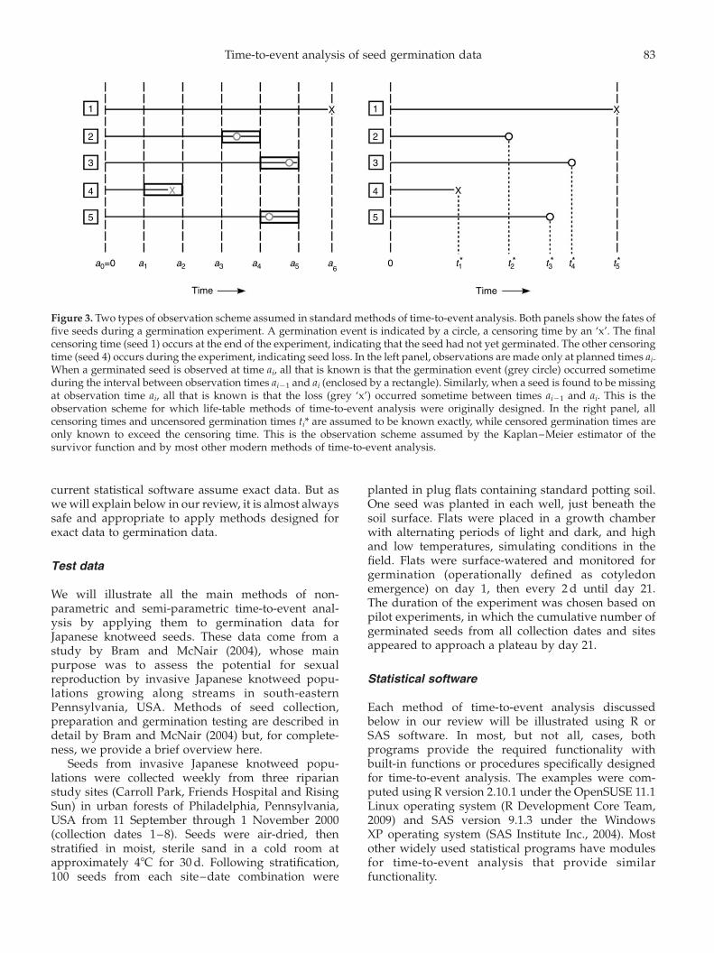
An observation scheme is a temporal pattern of seedmonitoring. A variety of observation schemes areemployed in different applications of time-to-eventanalysis (see Lawless, 2003), but two types areimportant to know about when analysing germinationdata. We call these periodic simultaneous observation andcontinuous observation, and we call the correspondingtypes of data interval data and exact data.
Periodic simultaneous observation and interval data
The observation scheme employed in standardgermination experiments is illustrated in the leftpanel of Fig. 3 and can be described as follows.All seeds are placed in an incubator at the sametime and are then observed at predetermined times0 ¼ a0 , a1 , a2 , a3 , · · · , am , 1. At each obser-vation time ai, all seeds are examined, and those whoseradicles are protruding are recorded as havinggerminated in the interval (ai21, ai] and are discarded.Care is taken to ensure that the amount of timerequired to check all seeds is negligible compared tothe length of time ai 2 ai21 between successiveobservation times. If any seeds are lost or damagedbetween observations ai21 and ai, the number isrecorded and assigned to interval (ai21, ai]. Thenumber of ungerminated seeds remaining at the(predetermined) final observation time am is alsorecorded. Germination times of these seeds are onlyknown to exceed am and so are right-censored.
We call this observation scheme ‘periodic simul-taneous observation’ because seeds are observedperiodically rather than continuously, and because allobservations are, to a good approximation, simul-taneous. We call the data that are produced ‘intervaldata’ because they represent the numbers of germina-tion events (and sometimes, seed losses) occurringwithin the various time intervals.
Continuous observation and exact data
The continuous observation scheme is illustratedin the right panel of Fig. 3 and can be described asfollows. As with periodic simultaneous observation,the germination experiment begins by placing all seedsin an incubator at the same time. Now, however, weassume that every seed is continuously monitored.If any seeds are lost during the experiment, we assumethe exact loss times are known. For lost seeds, all weknow regarding germination is that the germinationtime is greater than the loss time, so the germinationtime is right-censored. Of the seeds not lost, somemight not germinate by the (predetermined) end of theexperiment, so the time to germination will be right-censored for these seeds, as well. All the remainingseeds will germinate during the experiment, and weassume their germination times are known exactly.
For obvious reasons, we call this observationscheme ‘continuous observation’. And since the datafor seeds that germinate during the experimentrepresent exact germination times, we call them‘exact data’.
While data generated by standard germinationexperiments clearly are of the interval type, it issometimes necessary or desirable to analyse themusing statistical methods designed for exact data. Themain reason is that most of the methods available in
J.N. McNair et al.82
current statistical software assume exact data. But aswe will explain below in our review, it is almost alwayssafe and appropriate to apply methods designed forexact data to germination data.
Test data
We will illustrate all the main methods of non-parametric and semi-parametric time-to-event anal-ysis by applying them to germination data forJapanese knotweed seeds. These data come from astudy by Bram and McNair (2004), whose mainpurpose was to assess the potential for sexualreproduction by invasive Japanese knotweed popu-lations growing along streams in south-easternPennsylvania, USA. Methods of seed collection,preparation and germination testing are described indetail by Bram and McNair (2004) but, for complete-ness, we provide a brief overview here.
Seeds from invasive Japanese knotweed popu-lations were collected weekly from three riparianstudy sites (Carroll Park, Friends Hospital and RisingSun) in urban forests of Philadelphia, Pennsylvania,USA from 11 September through 1 November 2000(collection dates 1–8). Seeds were air-dried, thenstratified in moist, sterile sand in a cold room atapproximately 48C for 30 d. Following stratification,100 seeds from each site–date combination were
planted in plug flats containing standard potting soil.One seed was planted in each well, just beneath thesoil surface. Flats were placed in a growth chamberwith alternating periods of light and dark, and highand low temperatures, simulating conditions in thefield. Flats were surface-watered and monitored forgermination (operationally defined as cotyledonemergence) on day 1, then every 2 d until day 21.The duration of the experiment was chosen based onpilot experiments, in which the cumulative number ofgerminated seeds from all collection dates and sitesappeared to approach a plateau by day 21.
Statistical software
Each method of time-to-event analysis discussedbelow in our review will be illustrated using R orSAS software. In most, but not all, cases, bothprograms provide the required functionality withbuilt-in functions or procedures specifically designedfor time-to-event analysis. The examples were com-puted using R version 2.10.1 under the OpenSUSE 11.1Linux operating system (R Development Core Team,2009) and SAS version 9.1.3 under the WindowsXP operating system (SAS Institute Inc., 2004). Mostother widely used statistical programs have modulesfor time-to-event analysis that provide similarfunctionality.
1
2
3
4
5
1
2
3
4
5
a0=0 0 t1* t2* t3* t4* t5*
Time Time
a1 a2 a3 a4 a5 a6
X
X
X
X
Figure 3. Two types of observation scheme assumed in standard methods of time-to-event analysis. Both panels show the fates offive seeds during a germination experiment. A germination event is indicated by a circle, a censoring time by an ‘x’. The finalcensoring time (seed 1) occurs at the end of the experiment, indicating that the seed had not yet germinated. The other censoringtime (seed 4) occurs during the experiment, indicating seed loss. In the left panel, observations are made only at planned times ai.When a germinated seed is observed at time ai, all that is known is that the germination event (grey circle) occurred sometimeduring the interval between observation times ai21 and ai (enclosed by a rectangle). Similarly, when a seed is found to be missingat observation time ai, all that is known is that the loss (grey ‘x’) occurred sometime between times ai21 and ai. This is theobservation scheme for which life-table methods of time-to-event analysis were originally designed. In the right panel, allcensoring times and uncensored germination times ti* are assumed to be known exactly, while censored germination times areonly known to exceed the censoring time. This is the observation scheme assumed by the Kaplan–Meier estimator of thesurvivor function and by most other modern methods of time-to-event analysis.
Time-to-event analysis of seed germination data 83

Non-parametric time-to-event analysis ofgermination data
Two main problems can be addressed with non-parametric methods: characterizing the temporalpattern of germination within individual groups ofseeds, and comparing patterns of germination indifferent groups. For each problem, two main classesof methods are available, according as the data areassumed to be of interval or exact type.
Characterizing the temporal pattern ofgermination
Non-parametric methods of time-to-event analysisallow one to obtain quantitative estimates of thesurvivor function without assuming a particularfunctional form. Information that can be obtainedwith standard statistical software includes, forexample, the estimated survivor function and point-wise confidence intervals.
Interval data
Long before the emergence of time-to-event analysis asa statistical discipline in its own right, methods forestimating the survivor function for human popu-lations were developed by actuaries as part of theprocedure for constructing life tables. These methodsemployed census data and therefore assumed periodicsimultaneous observation and interval data. Becauseof its origin, the most commonly used method of thistype for estimating the survivor function is usuallycalled the life-table or actuarial estimator, which wenow describe.
The observation scheme for interval data isillustrated in the left panel of Fig. 3. Let the initialnumber of seeds be N. Given observation times0 ¼ a0 , a1 , a2 , · · · , am , 1, let the intervalsbetween observations be Ij ¼ (aj21, aj] for j ¼ 1, 2, 3,. . ., m. We assume the Ij are long enough relative tothe rate at which germination events occur so thatmultiple events commonly occur within an interval.Let Dj be the number of germination events occurringwithin interval Ij. We assume Dj is known but the exactevent times are not. Finally, let Ni be the number ofseeds at risk of germination (i.e. not yet germinatedor lost) at the beginning of interval Ii, with N1 ¼ N.
If no seeds are lost before the end of the experiment,then the standard life-table estimator SðajÞ of thesurvivor function at the observation times ai is given by
SðajÞ ¼Yj
i¼1
ð1 2 Di=NiÞ: ð5Þ
On the other hand, if seed losses do occur before the endof the experiment, it is necessary to adjust the Ni toaccount for the fact that because lost seeds cannot
contribute to the observed number of germinationevents during an interval, they effectively reduce thenumber of seeds at risk below Ni. Letting Ni
0 denotethe adjusted or effective number of seeds at risk, theresulting estimator of the survivor function is
SðajÞ ¼Yj
i¼1
ð1 2 Di=Ni0Þ; ð6Þ
where it remains to specify Ni0. The traditional choice
of Ni0, and the one implemented in standard statistical
software, is
Ni0 ¼ Ni 2 0:5Wi; ð7Þ
where Wi is the number of losses during interval Ii.Derivations of the above formulas are straightforwardand can be found in, for example, Elandt-Johnson andJohnson (1980), Lawless (2003), and Lee and Wang(2003).
Equations (5), (6) and (7) tell us how to estimate thesurvivor function at the observation times, but how dowe estimate its value at intermediate times? Recallingthat the observation times are chosen in such a waythat multiple events will occur in many of the intervalsbetween observations, it is most reasonable to assumeevents occur more or less uniformly during eachinterval Ii and therefore to estimate S(t) for ai , t , aiþ1
simply by linearly interpolating between S aið Þ andS aiþ1
� �. This is the result obtained by plotting the
estimated survivor function S aið Þ versus observationtimes ai and choosing the graphics option to connecteach pair of successive points with a straight line.
Methods are available in standard statistical soft-ware for estimating various other functions of interest,including the probability density function, hazardfunction and corresponding point-wise 95% confi-dence limits. Neither R nor SAS currently reports themedian or other quantiles for the life-table estimate ofthe survivor function, but the required methods arestraightforward (see Lee and Wang, 2003).
Figure 4 shows life-table estimates of survivorfunctions computed for the three study sites in thetest data using R function lifetab() from theKMsurv package. Examples are plotted for collectiondates 3 and 8, without (panels A and B) and with(panels C and D) point-wise 95% confidence intervals.lifetab() creates an object whose componentsinclude estimates and point-wise standard errors ofthe survivor function, probability density function andhazard function. Plots like those of Fig. 4 must becreated from this object using the default R plotfunction. Various types of point-wise 95% confidenceintervals can be constructed using the Greenwoodstandard errors created by lifetab(). Those in Fig. 4assume a normal distribution of SðaiÞ: SðaiÞ^ 1:96 SEi,where SEi is the standard error of SðaiÞ.
J.N. McNair et al.84

The SAS procedure lifetest also allows one toestimate life-table survivor functions, but it isimportant to note that it does so incorrectly forinterval data generated by periodic simultaneousobservation unless the data or observation times areadjusted so that the values entered as event times areslightly less than the observation times (see the onlinesupplementary material, available at http://journals.cambridge.org/).
Sample R and SAS code for estimating the survivorfunction using methods for interval data is providedin the supplementary material.
Exact data
Estimates of the survivor function when event timesare assumed to be exact (but with ties permitted) areusually obtained with the Kaplan–Meier estimator.The origin of this estimator can be traced back to theproduct-limit estimator of Bohmer (1912) in theactuarial literature. It is sometimes called the pro-duct-limit estimator in the statistical literature, but
Kaplan and Meier (1958) provided the first derivationbased on modern statistical concepts.
The Kaplan–Meier estimator of the survivorfunction is designed for exact data produced by acontinuous monitoring scheme, as illustrated in theright panel of Fig. 3. Let t1
*, t2*, t3
*, . . ., tN* denote the times
at which the N initial seeds either germinate or arecensored (including censoring by termination of theexperiment and seed loss), and let d1, d2, d3, . . ., dN bestatus variables that tell us whether the correspondingti
* values are germination times (di ¼ 1) or censoringtimes (di ¼ 0). (Note: in data files used for analysingdata that are treated as exact, every seed is representedby its pair of ti
* and di values.) We allow the possibilitythat some of the ti
* are identical, in which case thedata contain ties. Let t1 , t2 , t3 , · · · , tk (k # N) bethe distinct times at which germination events occur,and let dj be the number of germination events thatoccur at tj. Finally, let ni be the number of seedsthat were at risk of germination immediately prior to ti.Then the Kaplan–Meier estimator SðtÞ of the survivor
0.0
0.2
0.4
0.6
0.8
1.0
Time (days) Time (days)
Time (days) Time (days)
Pro
babi
lity
of n
ot g
erm
inat
ing
A
Site 1
Site 2
Site 3
0.0
0.2
0.4
0.6
0.8
1.0
Pro
babi
lity
of n
ot g
erm
inat
ing
C
0 5 10 15 20 0 5 10 15 20
0 5 10 15 20 0 5 10 15 20
0.0
0.2
0.4
0.6
0.8
1.0
Pro
babi
lity
of n
ot g
erm
inat
ing
B
0.0
0.2
0.4
0.6
0.8
1.0
Pro
babi
lity
of n
ot g
erm
inat
ing
D
Figure 4. Life-table estimates of survivor functions for Japanese knotweed seeds collected from three study sites on collectiondates 3 (left panels) and 8 (right panels), computed by R function lifetab() from the KMSurv package. The lower panels arethe same as the upper panels, except that point-wise 95% confidence intervals (thin lines) have been added. Confidence intervalsare based on a normal approximation using Greenwood standard errors computed by lifetab(); see text for details.
Time-to-event analysis of seed germination data 85

function is given by
SðtÞ ¼i:ti,t
Y ni 2 di
ni
� �¼
i:ti,t
Yð1 2 di=niÞ; ð8Þ
where i is the index of the observed germination times.(For derivations, see Cox and Oakes, 1984; Lawless,2003.) Note that SðtÞ is a step function that changes(decreases) only at values of t at which germinationevents occur, and that the effect of seed loss is toreduce nj.
How do the Kaplan–Meier and life-table estimatesof the survivor function compare when they areapplied to the same germination data? For standardgermination experiments, the data will be of intervalrather than exact type, so we apply the Kaplan–Meierestimator by treating the actual observation times ai asif they were infinitesimally greater than the unknowngermination times ti for intervals in which germinationevents occurred. We also treat the known number Di
of germination events in interval Ii as if it were thenumber di of (tied) events occurring at distinct eventtime ti, and we treat the known number Ni of seeds atrisk at the beginning of interval Ii as the number ni
at risk immediately prior to event time ti. At theactual observation times, then, the Kaplan–Meierestimator is
SðajÞ ¼i:ti,aj
Y ni 2 di
ni
� �¼
Yj
i¼1
ð1 2 Di=NiÞ: ð9Þ
Comparing equation (9) with equation (8), we seethat the values of the Kaplan–Meier and life-tablesurvivor functions will be identical at the observationtimes when there are no seed losses. When seed lossesoccur, the two estimators will differ (because theyaccount for losses differently), but numerical examplessuggest that they will be very similar at theobservation times if the proportion of seeds lost isless than roughly 5%. This is not much of a restriction,since 5% seed loss would normally be consideredunacceptable for other reasons and the experimentwould be repeated.
Standard statistical software also provides methodsfor estimating various other quantities and functionsassociated with the distribution of germination time,such as the median, probability density function andhazard functions, plus corresponding confidenceintervals. Since the Kaplan–Meier estimator producesa step function, there typically will not be an estimatedvalue that exactly corresponds to the median (or otherquantile). The usual estimate of the median is thesmallest event time ti such that SðtiÞ , 0:5.
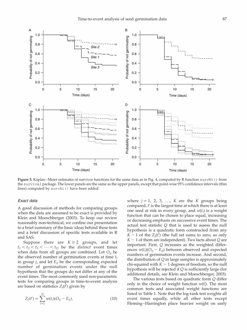
Figure 5 shows Kaplan–Meier survivor functionscomputed for the three study sites in the test datausing R function survfit() from the survivalpackage. These functions are shown for collection
dates 3 and 8 without (panels A and B) and with(panels C and D) point-wise 95% confidence intervals.The survfit() function also creates tabular outputthat is stored in an object whose fields includeestimates of the median and 95% confidence limits ofthe time to germination, as well as the survivorfunction and its point-wise standard errors and 95%confidence limits. SAS procedure lifetest also canbe used to plot Kaplan–Meier survivor functions andto create corresponding tabular output.
Sample R and SAS code for estimating the survivorfunction using methods for exact data is provided inthe online supplementary material.
Comparing groups
The estimated survivor functions with point-wiseconfidence intervals in Figs 4 and 5 suggest that thetemporal pattern of germination is different for allthree study sites for seeds collected on date 3. Forseeds collected on date 8, however, the figures suggestthat the pattern is the same for sites 1 and 3 butdifferent for site 2. Time-to-event analysis providesseveral non-parametric techniques for rigorouslytesting such hypotheses regarding potential groupdifferences in the temporal pattern of germination.One can test for homogeneity of a set of three or moregroups, or conduct pairwise tests to determinewhether specific pairs of groups are statisticallysignificantly different, all without assuming a para-metric form for the survivor function.
Interval data
At the time of this writing, neither R nor SAS providesinterval-data methods for comparing life-table survi-vor functions. For this reason, we relegate discussionof these methods to the supplementary material. Wenote, however, that both R and SAS include an exact-data version of the Mantel–Haenszel test (the maininterval-data test; see the supplementary material) thatis usually called the log-rank test. When applied tostandard germination data, the log-rank test will givethe same results as the Mantel–Haenszel test if thereare no seed losses. When a small proportion of seedsare randomly lost, the values of the test statisticsusually will remain very similar. Therefore, providedseed loss is absent or rare (e.g. roughly 5% or less), theR or SAS log-rank test can be used for comparinggroups in germination experiments, even though thedata are of interval rather than exact type.
Several other common methods for comparinggroups with exact data are straightforward extensionsof the log-rank test. Because of their fundamentalsimilarity to the log-rank test, we argue that it is alsoappropriate to analyse germination data using theseother exact-data tests, which we describe next.
J.N. McNair et al.86
Exact data
A good discussion of methods for comparing groupswhen the data are assumed to be exact is provided byKlein and Moeschberger (2003). To keep our reviewreasonably non-technical, we confine our presentationto a brief summary of the basic ideas behind these testsand a brief discussion of specific tests available in Rand SAS.
Suppose there are K $ 2 groups, and lett1 , t2 , t3 , · · · , tD be the distinct event timeswhen data from all groups are combined. Let Oij bethe observed number of germination events at time ti
in group j, and let Eij be the corresponding expectednumber of germination events under the nullhypothesis that the groups do not differ at any of theevent times. The most commonly used non-parametrictests for comparing groups in time-to-event analysisare based on statistics Zj(t
0) given by
Zjðt0Þ ¼
XD
i¼1
wðtiÞðOij 2 EijÞ; ð10Þ
where j ¼ 1, 2, 3, . . ., K are the K groups beingcompared, t0 is the largest time at which there is at leastone seed at risk in every group, and w(ti) is a weightfunction that can be chosen to place equal, increasingor decreasing emphasis on successive event times. Theactual test statistic Q that is used to assess the nullhypothesis is a quadratic form constructed from anyK 2 1 of the Zj(t
0) (the full set sums to zero, so onlyK 2 1 of them are independent). Two facts about Q areimportant. First, Q increases as the weighted differ-ences w(ti)(Oij 2 Eij) between observed and expectednumbers of germination events increase. And second,the distribution of Q in large samples is approximatelychi-squared with K 2 1 degrees of freedom, so the nullhypothesis will be rejected if Q is sufficiently large (foradditional details, see Klein and Moeschberger, 2003).
The various tests based on quadratic form Q differonly in the choice of weight function w(t0i). The mostcommon tests and associated weight functions arelisted in Table 1. Note that the log-rank test weights allevent times equally, while all other tests exceptFleming–Harrington place heavier weight on early
0 5 10 15 20 0 5 10 15 20
0.0
0.2
0.4
0.6
0.8
1.0
Time (days)
Pro
babi
lity
of n
ot g
erm
inat
ing
A
C
B
D
Site 1
Site 2
Site 3
0.0
0.2
0.4
0.6
0.8
1.0
Pro
babi
lity
of n
ot g
erm
inat
ing
0.0
0.2
0.4
0.6
0.8
1.0
Time (days)
0 5 10 15 20 0 5 10 15 20
Time (days) Time (days)
Pro
babi
lity
of n
ot g
erm
inat
ing
0.0
0.2
0.4
0.6
0.8
1.0
Pro
babi
lity
of n
ot g
erm
inat
ing
Figure 5. Kaplan–Meier estimates of survivor functions for the same data as in Fig. 4, computed by R function survfit() fromthe survival package. The lower panels are the same as the upper panels, except that point-wise 95% confidence intervals (thinlines) computed by survfit() have been added.
Time-to-event analysis of seed germination data 87

event times (for which there are the most data) than onlate event times. The Fleming–Harrington test is veryflexible and is the only test capable of weighting lateevent times more heavily than early event times. It isconvenient to refer to all these tests as generalized log-rank tests. They are best viewed as tests for differencesin hazard rate, since the number of seeds at risk in eachgroup at each event time is regarded as fixed.
Methods for comparing the survival patterns fortwo or more groups with data assumed to be exact (butwith ties allowed) are available in both R (functionsurvdiff() in package survival) and SAS(procedure lifetest), and sample code for bothsoftware programs is provided in the supplementarymaterial. At the time of this writing, R functionsurvdiff() provides only the Fleming–Harringtontest with b ¼ 0, which specializes to the log-rank testwhen a ¼ 0 and is similar (but not identical) to thePeto–Peto test when a ¼ 1. (Parameters a and b aredefined in Table 1.) SAS procedure lifetestcurrently provides all the tests listed in Table 1.
Table 2 shows examples of results computed withSAS procedure lifetest for collection dates 3 and 8in the test data. For each collection date, results areshown for tests of homogeneity of the three sites,followed by results of the three possible pair-wisetests. Note that, as suggested by Fig. 5, and regardlessof which test is employed, the three sites arestatistically significantly different from each other oncollection date 3, whereas sites 1 and 3 differ from site2 but not from each other on collection date 8.
The issue of replicates
It will be noted that we did not mention experimentalreplicates in connection with any of the non-parametric methods discussed above. The reason is
that replication is not necessary for rigorous time-to-event analysis and, indeed, is almost never used inmedical applications. If replicates are employed, thedata normally would be combined within treatmentswhen using non-parametric methods of time-to-eventanalysis. An extension to semi-parametric and fullyparametric methods allows one to assess randomvariation among replicates using so-called frailtymodels (discussed below), but these models areparametric and thus incompatible with non-para-metric methods.
Semi-parametric time-to-event analysis ofgermination data
The main benefit of semi-parametric methods of time-to-event analysis is that they allow one to assesspotential effects of multiple covariates, including bothcategorical and quantitative covariates, while still notrequiring one to assume a fully parametric form for thesurvivor function. In medical applications of time-to-event analysis, the semi-parametric Cox model ‘hasbecome by a wide margin the most used procedure formodeling the relationship of covariates to a survivalor other censored outcome’ (Therneau and Grambsch,2000, p. 39), and it is the only semi-parametricapproach that is well supported by standard statisticalsoftware. For these reasons, the Cox model is the onlysemi-parametric method we will discuss.
The Cox model is robust, flexible, extensible andreasonably powerful; it can accommodate categoricaland quantitative covariates with fixed effects, it canaccommodate random effects and it requires fewparametric assumptions. We therefore think it hasgreat potential as a tool for statistical analysis ofgermination data. We treat this method at greaterlength than the others, because applying the Coxmodel requires more steps, and the manner in whichresults of the analysis are interpreted will beunfamiliar to most biologists.
The Cox proportional hazards model
The Cox model is based on the hazard function ratherthan the survivor function. The basic idea behind themodel is that the hazard function h(tjx) at time t, givena vector x ¼ [xi] of covariates, can be expressed as theproduct of a baseline hazard function that dependsonly on time, and a modifier function that dependsonly on the covariates. That is,
hðtjxÞ ¼ h0ðtÞcðbTxÞ
¼ h0ðtÞ expðb1x1 þ b2x2 þ · · · þ bkxkÞ; ð11Þ
where h0(t) is the baseline hazard function (whoseform need not be specified; see below), xi is the i-th
Table 1. Common non-parametric tests for determiningwhether two or more survival functions are statisticallysignificantly different (modified from Table 7.3 of Klein andMoeschberger, 2003). The associated weight function isshown for each test. Notation: ni is the total number of seedsat risk immediately prior to distinct event time ti, S isKaplan–Meier estimator (equation 8) of the text, ~S is thesame except that product terms 1 2 di/ni are replaced by1 2 di/(ni þ1) where di is the total number of observedgermination events at ti, and a and b are non-negativeparameters
Test Weight function, w(ti)
Log-rank 1.00Gehan ni
Tarone–Wareffiffiffiffini
p
Peto–Peto ~SðtiÞ
Modified Peto–Peto ~SðtiÞni=ðni þ 1ÞFleming–Harrington Sðti21Þ
a½1 2 Sðti21Þ�b
J.N. McNair et al.88

covariate, bi is the slope coefficient for the i-thcovariate, b and x are the vectors [bi] and [xi], and c
is a function that typically is taken to be theexponential function, as in equation (11). An importantadvantage of the Cox model over non-parametricmethods is that it permits quantitative covariates.Categorical covariates are also permitted, and these arecoded using indicator (or ‘dummy’) variables, as inordinary least-squares regression.
The bi coefficients in equation (11) captureinformation about the relationship between thecorresponding covariates and the hazard function.One can see that this model has a feel similar to anordinary regression model. It is called semi-parametricbecause no parametric assumptions are made aboutthe baseline hazard function, while the covariateportion does depend on parameters. In this most basicform of the Cox model, it is assumed that none of the bi
or xi depends on time, though this assumption can berelaxed in extensions of the model (see Cox and Oakes,1984; Therneau and Grambsch, 2000; Klein andMoeschberger, 2003; Lawless, 2003).
Just as in ordinary regression, the goal is to estimatethe bi and then test to see if they are significantlydifferent from 0. Estimation of the bi is done through aprocess called partial likelihood, which is similar to themore traditional likelihood approaches seen in othercontexts. In its pure form, this process assumes strictcontinuous observation and exact data and thereforedoes not accommodate tied event times. However,even in medical applications for which the Cox modelwas originally developed, tied event times are verycommon, and modifications of partial likelihoodestimation have therefore been developed to accom-modate them. Standard statistical software typicallyincludes at least two such modifications: the Breslowmethod and the Efron method (see Therneau and
Grambsch, 2000). For germination data, where ties arecreated by the observation scheme, we recommend theEfron method, which provides a good combination ofaccuracy and computational speed.
A highly desirable feature of the Cox model isthat the bi have an easily understood interpretation.They are related to what is commonly called thehazard ratio. To understand the interpretation,consider a categorical covariate x1 with two levels,coded as 1 and 0. Suppose we have an estimate ofthe corresponding slope coefficient b1, denoted by b1.Then the hazard ratio (HR) for one group relative tothe other is
HR ¼hðtjx1 ¼ 1Þ
hðtjx1 ¼ 0Þ¼
h0ðtÞ exp ðb1�1Þ
h0ðtÞ exp ðb1�0Þ
¼ exp ðb1Þ: ð12Þ
Suppose that exp ðb1Þ ¼ 2. This means that thehazard function for the first group is twice as largeas that for the second group. Therefore, a seed thathas not germinated by time t is twice as likely togerminate in the next short interval of time if itcomes from group 1 than if it comes from group 2.
Note that the baseline hazard function cancelsfrom the hazard ratio in equation (12). The hazard ratiotherefore is constant with respect to time, which is whythe Cox model is called the proportional hazardsmodel. This is an important assumption of the Coxmodel and should be checked. There are a variety ofways to do so, including graphical methods as well asformal tests (e.g. see Andersen et al., 1993; Therneauand Grambsch, 2000; Klein and Moeschberger, 2003;Lawless, 2003). We prefer graphical methods forseveral reasons. Most importantly, because theproportional hazards (PH) assumption will always
Table 2. Results of group (site) comparisons for seeds collected on dates 3 and 8, illustrating the six tests listed in Table 1. Testswere performed with SAS procedure lifetest using the default parameter values for the Fleming–Harrington test (a ¼ b ¼ 1).The three p values for each pairwise test are Holm-adjusted for multiple comparisons
Collectiondate
All 3 sites Sites 1 and 2 Sites 2 and 3 Sites 1 and 3
Test x2 df P x2 df P x2 df p x2 df p
3 Log-rank 41.3592 2 ,0.0001 13.2885 1 0.0005 42.4257 1 ,0.0001 8.5253 1 0.0035Gehan 36.7898 2 ,0.0001 12.9392 1 0.0006 38.0188 1 ,0.0001 6.4840 1 0.0109Tarone–Ware 39.2321 2 ,0.0001 13.1408 1 0.0006 40.3715 1 ,0.0001 7.5672 1 0.0059Peto–Peto 37.0767 2 ,0.0001 13.1667 1 0.0006 38.5764 1 ,0.0001 6.2002 1 0.0128Modified Peto–Peto 37.0556 2 ,0.0001 13.1640 1 0.0006 38.5451 1 ,0.0001 6.1864 1 0.0129Fleming–Harrington 36.7898 2 ,0.0001 12.9392 1 0.0006 38.0188 1 ,0.0001 6.4840 1 0.0109
8 Log-rank 87.2988 2 ,0.0001 62.6100 1 ,0.0001 67.6390 1 ,0.0001 0.6469 1 0.4212Gehan 68.3086 2 ,0.0001 49.7664 1 ,0.0001 58.1806 1 ,0.0001 1.3391 1 0.2472Tarone–Ware 78.7124 2 ,0.0001 56.4034 1 ,0.0001 63.6780 1 ,0.0001 1.1937 1 0.2746Peto–Peto 64.5875 2 ,0.0001 47.5383 1 ,0.0001 55.3658 1 ,0.0001 1.3544 1 0.2445Modified Peto–Peto 64.4563 2 ,0.0001 47.4295 1 ,0.0001 55.2718 1 ,0.0001 1.3578 1 0.2439Fleming–Harrington 68.3086 2 ,0.0001 49.7664 1 ,0.0001 58.1806 1 ,0.0001 1.3391 1 0.2472
Time-to-event analysis of seed germination data 89

be a simple approximation to a pattern that is morecomplex in reality, it is virtually certain that thisassumption will be rejected by a formal test if thesample size is sufficiently large, even if it provides areasonable approximation (as Klein and Moeschber-ger, 2003, point out). On the other hand, a formal testcan easily accept the PH assumption if the sample sizeis small, even if it provides a poor approximation,since the null hypothesis is that the assumption is met.
A common graphical method of testing the PHassumption, available in both R and SAS, is to plot2logð2logðSðtjxÞÞÞ versus t or log(t) for differentvalues of covariate vector x (restricted to values oft such that 0 , S(t) , 1), where S(t) is a life-table orKaplan–Meier survivor function. Under the PHassumption, different covariate values will producefunctions with the same shape but different elevations(see the supplementary material). The Cox model isreasonably robust, so it is only necessary to worryabout clear departures from proportionality, asindicated by decisive crossing of the functions fortwo or more covariates in the diagnostic plot.
When clear violations of the PH assumption aredetected, various remedies are available in standardstatistical software that may resolve the problem andstill permit use of the Cox model. These includeconverting covariates with non-proportional effectsinto stratification factors or time-dependent covariates,and dividing the time axis into discrete segments andanalysing data for one or more of the segmentsseparately (see Therneau and Grambsch, 2000).
In applications of the Cox model, there typicallywill be several covariates that are viewed as potentiallyimportant prior to analysing the data. But how dowe rigorously assess the actual importance of thesecovariates? In other words, how do we determinewhich covariates should be included in the Cox modeland which should be excluded?
We suggest a model-building procedure similarto ones employed with ordinary multivariableregression models. As an initial exploratory technique,we suggest using a non-parametric method (e.g.Kaplan–Meier) to estimate and plot survivor functionsfor different values of the covariates, as shown in Figs 4and 5 for three study sites and two collection dates inthe Japanese knotweed data. Next, the PH assumptionshould be assessed for different values of thecovariates, and any remedies required by clearviolations should be applied. An example for theJapanese knotweed test data is shown in Fig. 6, where2logð2logðSðtjxÞÞÞ versus log(t) is plotted for differentstudy sites (left panel) and for early versus latecollection dates (right panel), based on Kaplan–Meiersurvivor functions. These plots show no evidence ofdecisive crossing of the transformed survivor func-tions, so the PH assumption is plausible for allcovariates. Potential multicollinearity of the covariates
should also be assessed in the initial phase of analysis,using the same methods (e.g. variance inflation factor)that are used in standard multiple regression analysis(Ryan, 1997; Draper and Smith, 1998; Montgomeryet al., 2001; Belsley et al., 2004; Kutner et al., 2004).
For the model-building process, categorical covariatesare coded using indicator variables, while quantitativecovariates are used unchanged. For example, in theJapanese knotweed data, study site is categorical withthree categories, so we may define two indicatorvariables, x1 and x2, as follows:
x1 ¼1; if site ¼ Friends
0; otherwise:
(x2 ¼
1; if site ¼ RisingSun
0; otherwise:
(
ð13Þ
(Note that x1 ¼ x2 ¼ 0 implies that site ¼ Carroll.)Collection date is a quantitative variable and thereforecan be inserted in the Cox model as a single covariate,x3. Model building begins by putting one covariate at atime into the Cox model and checking the reportedp value for the null hypothesis that bi ¼ 0. Covariatesfor which p is sufficiently small (e.g. p , 0.05) arecandidates for use in building up a multivariablemodel. This is done in exactly the same manner as inordinary multivariable regression, using an automaticselection procedure (though we do not advocate usingthese by themselves), the Akaike Information Criterion(AIC), p values and so forth. Interaction terms can alsobe added to the model, provided there is a meaningfulbasis for them. Ultimately, one arrives at a Cox modelthat may have multiple covariates in it, and the hazardratios can be interpreted.
For the Japanese knotweed test data, a forward-selection procedure based on p values produces a finalCox model that includes all three covariates (x1, x2, x3)but no pair-wise interactions. Table 3 summarizes themodel, including the estimated values of coefficientsb1, b2 and b3. The hazard function has the form
hðtjxÞ ¼ h0ðtÞexpð21:276x1 þ 0:144x2 þ 0:330x3Þ;
ð14Þ
where covariates x1 and x2 are indicator variables forstudy sites Friends and Rising Sun, and x3 is collectiondate.
We illustrate interpretation of this model byconsidering the effect of study site Friends. (Acomplete interpretation of the model is provided inthe supplementary material.) To assess the effect ofstudy site Friends on germination time while control-ling for (or removing) effects of collection date, weconsider the ratio of the hazard function with x1 ¼ 1,x2 ¼ 0 and x3 taking on any admissible value (in thenumerator), to the hazard function with x1 ¼ x2 ¼ 0and x3 constrained to the same value as in thenumerator (in the denominator). The resulting hazard
J.N. McNair et al.90

ratio is
HR ¼ expð21:276Þ ¼ 0:28: ð15Þ
Choosing x1 ¼ 1 and x2 ¼ 0 for any x3 implies that thenumerator applies to the Friends site for any chosencollection date, while choosing x1 ¼ 0 and x2 ¼ 0 withthe same value of x3 implies that the denominatorapplies to the Carroll site for the same collection date.Thus, the hazard ratio in equation (15) indicates thatfor any given collection date, seeds from the Friendssite have a hazard function for germination that is 0.28times (28%) as large as the hazard function for seedsfrom the Carroll site. This shows that the slopecoefficient for Friends implicitly specifies the effect ofFriends relative to Carroll. Recalling equation (4), thisresult indicates that for any given collection date, thesurvivor function for seeds from Friends will begreater than the survivor function for seeds fromCarroll, and therefore seeds from Friends will tend togerminate later than seeds from Carroll.
Both R and SAS include dedicated modules forimplementing the Cox model. The main function in Ris coxph() in the survival package; the mainprocedure in SAS is phreg. Code examples for R andSAS are provided in the supplementary material,along with an example illustrating all the steps inbuilding a multivariate Cox model for the Japaneseknotweed test data.
Including random effects
The non-parametric and semi-parametric methods wehave considered until now assume that covariateshave fixed effects. But just as in ordinary least-squaresregression, it is often desirable to include a randomeffect in the Cox model. For reasons that are somewhatarcane, random effects are called frailty effects in time-to-event analysis.
The most common situation in germination studieswhere inclusion of a frailty effect may be desirable iswhere there are subgroups within treatment groups,such that seeds within a subgroup have approximatelythe same hazard function while seeds in differentsubgroups of a treatment group may have slightlydifferent hazard functions. An example is experimentswith replicates, where conditions experienced by seedsin the same replicate (e.g. the same Petri dish) maybe more similar than those experienced by seeds indifferent replicates, resulting in random differences ingermination properties among replicates. Anotherexample is experiments in which the subgroups withintreatment groups consist of seeds from the sameindividual plant, which might be more similar thanseeds from different individual plants. This type offrailty is often called shared frailty, because allindividuals in the same subgroup share the samelevel of frailty.
5 10 15 20 5 10 15 20
0
1
2
3
4
t (days) t (days)
–log
(–lo
g(S
(t))
)Site 2
Site 3
Site 1
0
1
2
3
4
–log
(–lo
g(S
(t))
)
Early
Late
Figure 6. Diagnostic plots for assessing the proportional-hazards assumption of the Cox model. Both panels show plots of2logð2logðSðtjxÞÞÞ versus t, with t on a logarithmic scale. The left panel shows Kaplan–Meier curves for the three study sites,with data for all eight collection dates combined. The right panel shows curves for early and late collection dates (dates 1–4 and5–8), with data for all sites combined.
Table 3. Summary table of the final Cox model for the Japanese knotweed test data,as produced by R function coxph() in package survival. SE denotes thestandard error
Covariate, xi Coefficient, bi exp(bi) SE of bi z p
x1 (Friends) 21.276 0.279 0.0784 216.27 ,0.00001x2 (Rising Sun) 0.144 1.154 0.0610 2.36 0.01847x3 (Collection Date) 0.330 1.391 0.0126 26.18 ,0.00001
Time-to-event analysis of seed germination data 91

The most common method of including frailty inthe Cox model is the same, regardless of the number ofcovariates. In the case of shared frailty with a singlequantitative covariate, the Cox model for the i-thsubgroup can be written as
hðtjx;aiÞ ¼ aih0ðtÞexpðbxÞ; ð16Þ
where ai is the (random, unobserved) level of thefrailty for the i-th subgroup. We assume that ai issampled from some probability distribution but isconstant over time.
Unlike the case in ordinary least-squaresregression, the frailty effect is assumed to be multi-plicative rather than additive, as equation (16) shows.This means that among individuals with the samevalue of covariate x, those in subgroups with ai . 1 areat increased risk of experiencing the event relative tothose in subgroups with ai , 1. We therefore choose adistribution for the frailty effect that has a mean of 1rather than 0, so that ai ¼ 1 corresponds to ‘averagefrailty’. The most common choice is a gammadistribution, though any distribution defined on(0, 1) and having mean 1 can be used if it is supportedby software.
Frailty levels for subgroups or individuals areassumed to be sampled from a probability distributionand therefore typically are not estimated. Instead, wetake the variance of the frailty distribution to be anunknown parameter to be estimated, and we test thenull hypothesis that the variance parameter is equal tozero. If the null hypothesis is not rejected, then there isno strong evidence of variability in frailty levels andthe frailty effect is not retained in the model.
As when building a multivariable Cox modelwithout frailty, there is no single ‘best’ procedure forbuilding a multivariable model that addresses frailty.We suggest the following modification of the aboveprocedure for models without frailty. In the initialstage of model building, where fixed-effect covariatesare included one at a time, a frailty term should beincluded along with each individual covariate. If thefrailty term is found to be statistically significant in anyof these cases, then there is evidence that it isimportant and it should be included in all furthersteps of the model-building process, regardless of thesubsequent p values reported for the frailty term. Onthe other hand, if the frailty term is not found to besignificant with any of the individual covariates, thenit should no longer be considered in further steps ofthe model-building process.
Extra care must be taken with interpretation ofhazard ratios in models that include a frailty effect. Tosee this, consider a shared-frailty Cox model with asingle quantitative covariate x, and let ai denote thefrailty level for subgroup i (e.g. a replicate). Then thehazard ratio HR for covariate value x þ 1 in subgroup i
relative to covariate value x in subgroup j is
HR ¼h tjx þ 1;ai
� �h tjx;aj
� � ¼aih0ðtÞexpðbðx þ 1Þ
ajh0ðtÞexpðbxÞ
¼ai
ajexpðbÞ: ð17Þ
Clearly the hazard ratio depends on the frailty effectsunless ai ¼ aj. But as noted above, we typically willnot have estimates of ai and aj. Therefore, we mustwork with the hazard ratio by assuming ai ¼ aj (so thefrailty effects disappear) and interpret it as the effect ofa unit increase in the covariate based on twosubgroups with the same level of frailty.
At the time of this writing, SAS does not providebuilt-in procedures or options for including frailtyterms in Cox models. In contrast, the process is simplein R and is accomplished by using the frailty()function to specify a frailty term in the model formulaof the coxph() function.
We will use the Japanese knotweed test data toillustrate the process of building a multivariable Coxmodel that includes a frailty term. (Additional detailsand code examples can be found in the supplementarymaterial.) The Japanese knotweed data do not includereplicates, but for purposes of illustration, we createdartificial replicates as follows. Using an R script, werandomly assigned the 100 seeds in each of the 24treatment groups (8 collection dates £ 3 study sites) to5 subgroups of 20 seeds each. These 120 subgroups (24groups £ 5 subgroups per group) were then uniquelylabelled and treated as replicates.
Applying the modified model-building procedureoutlined above to these data, the first step is to includethe fixed-effect covariates in a Cox model one at a time,while also including a gamma-distributed shared-frailty term along with each individual fixed-effectcovariate. Each of the 120 replicates is assumed to besubject to a separate gamma-distributed random effectthat applies to all 20 seeds. We find that all threecovariates have significant effects ( p , 0.01 in all threecases), and that the frailty effect is highly significant( p , 0.000001 in all three cases). We therefore includethe frailty term in all remaining steps of building themodel. We then build a multivariable Cox model in thesame manner as before. The final model is summar-ized in Table 4. The main difference from the modelsummarized in Table 3 is that the covariate represent-ing the Rising Sun site is no longer included. Recallthat the germination pattern for this site is similar tothat at the Carroll Park site for later collection dates,and that the site slope coefficients in the modelrepresent effects relative to Carroll Park. Thus, randomvariation among replicates results in a loss of ability todetect a difference between the Rising Sun and CarrollPark sites.
J.N. McNair et al.92

Summary and discussion
The various non-parametric and semi-parametricmethods we have reviewed are summarized inTable 5. As can be seen by perusing this table, themost appropriate method depends on the questions ofinterest. If one is mainly interested in comparinggroups of seeds, then non-parametric methods are anappropriate choice. In exchange for reduced statisticalpower, these methods have the advantage of avoidingany dependence on parametric assumptions. If one isinterested in assessing effects of quantitative covari-ates on germination, such as temperature, duration ofseed storage or duration of stratification (and possiblycomparing groups, as well), then the semi-parametricCox model is appropriate. Semi-parametric methodsretain part of the advantage of non-parametericmethods by avoiding dependence on a fully para-metric germination – time distribution, but theinclusion of covariates requires parametric regression-like assumptions about the form and strength of theireffects. Fully parametric methods (not included in Table5) are required only if one needs additional statisticalpower to detect small effects or wishes to quantify theshape of the survivor function in detail.
We have noted that data from germinationexperiments typically have two properties thatdiffer from the norm in medical applications of time-to-event analysis for which most of the modernstatistical methods were developed: a non-negligibleinitial delay in the onset of germination and anunknown mixture of germinable and non-germinable
seeds. Implications of these properties regardingthe validity or interpretation of the various methodsof time-to-event analysis vary, as we now discussbriefly.
Neither of these properties of germination dataaffects the validity of non-parametric methods. Theydo, however, constrain the interpretation of anysignificant between-group differences that aredetected, since the statistical methods do not indicatewhether the detected differences are due to differencesin initial delay, proportion of non-germinable seeds,some other aspect of the survivor function’s shape orsome combination of these properties.
Presence of an unknown proportion of non-germinable seeds does not affect the validity of theCox model (Maller and Zhou, 1996), but in the sameway as for non-parametric methods, it constrains theinterpretation of any statistically significant covariateeffects. The delay in onset of germination ispotentially a more serious problem. The PH assump-tion cannot be strictly true in cases where thegermination delay differs among experimental treat-ments. But as long as graphical assessment of the PHassumption does not indicate a clear violation, theCox model will provide an acceptable approximation.The Japanese knotweed example illustrates this pointwell (see the supplementary material). If a clearviolation of the PH assumption is evident, one canresolve the problem by simply removing the delayfrom the recorded germination times for eachtreatment before applying the Cox model. Otherwise,the delay should be retained.
Table 4. Summary table of the final shared-frailty Cox model for the Japanese knotweed testdata, as produced by R function coxph() in package survival. SE denotes the standard error,Chisq denotes chi-squared (x2), and df denotes degrees of freedom
Covariate, xi Coefficient, bi exp(bi) SE of bi Chisq df p
x1 (Friends) 21.395 0.248 0.1220 131 1 ,0.00001x3 (Collection Date) 0.384 1.469 0.0262 216 1 ,0.00001Frailty — — — 252 79.7 ,0.00001
Table 5. Summary of the major non-parametric and semi-parametric methods of time-to-event analysis supported by R and SAS
Statistical method Test type Data type Main uses
Estimating the survivor functionLife-table estimator NP Interval Estimate survivor function and point-wise confidence intervalKaplan–Meier estimator NP Exact1 Estimate survivor function and point-wise confidence interval
Assessing fixed effects of categorical covariates (comparing groups)Generalized log-rank tests NP Exact1 Homogeneity test for multiple groups, pair-wise comparisonsCox model SP Exact1 Pair-wise comparisons based on hazard ratio
Assessing fixed effects of quantitative covariatesCox model SP Exact1 Estimate and assess significance of regression-like effects on hazard rate
Assessing fixed and random effects with categorical and quantitative covariatesCox model with frailty SP Exact1 Assess significance of random variation among subgroups
1
Ties are permitted; NP, non-parametric; SP, semi-parametric.
Time-to-event analysis of seed germination data 93

In principle, neither the initial delay in onsetof germination nor the presence of an unknownproportion of non-germinable seeds is problematicfor fully parametric methods. As in the non-linearregression approach, these properties are representedby model parameters whose values must be estimated.But these properties are fatal problems if one wishesto analyse germination data with built-in functions orprocedures of standard statistical software, becauseeach implies a distribution of germination time that isnot a member of the family of distributions permittedby current software (i.e. distributions that are membersof the location-scale family for some differentiable andinvertible transformation of germination time, suchas log(T)). It is not difficult to construct appropriatedistributions that include an initial delay and anunknown proportion of non-germinable seeds, butbecause such distributions are not accommodatedby standard software, it is necessary to write customcode in order to estimate model parameters, constructconfidence intervals and test hypotheses. Workingwithin a statistical programming environment suchas R makes these tasks reasonably straightforward,but the technical details are beyond the scope ofthis review.
Acknowledgements
The study from which our test data were taken wasfunded by a grant to J.N.M. from the William PennFoundation; Margot Bram conducted the germinationexperiments. A.S. was supported by a D.J. Angus-Scientech Educational Foundation Internship at theAnnis Water Resources Institute. Thanks to RogerLatham and the reviewers for helpful comments.
References
Andersen, P.K., Borgan, Ø., Gill, R.D. and Keiding, N.(1993) Statistical models based on counting processes.New York, Springer-Verlag.
Baskin, C.C. and Baskin, J.M. (2001) Seeds: Ecology,biogeography, and evolution of dormancy and germination.New York, Academic Press.
Baskin, J.M. and Baskin, C.C. (1983) Germination ecology ofVeronica arvensis. Journal of Ecology 71, 57–68.
Belsley, D.A., Kuh, E. and Welsch, R.E. (2004) Regressiondiagnostics: Indentifying influential data and sources ofcollinearity. New York, John Wiley and Sons.
Bohmer, P.E. (1912) Theorie der unabhangigen Wahrschein-lichkeiten. pp. 327–343 in Reports, Memoirs, and Proceed-ings of the Seventh International Congress of Actuaries,September 1912, Amsterdam, vol. 2.
Bonner, F.T. and Dell, T.R. (1976) The Weibull function: anew method of comparing seed vigor. Journal of SeedTechnology 1, 96–103.
Bram, M.R. and McNair, J.N. (2004) Seed germinability andits seasonal onset in three populations of Japaneseknotweed. Weed Science 52, 759–767.
Brown, R.F. (1987) Germination of Aristida armata underconstant and alternating temperatures and its analysiswith the cumulative Weibull distribution as a model.Australian Journal of Botany 35, 581–591.
Brown, R.F. and Mayer, D.G. (1988a) Representing cumu-lative germination. 1. A critical analysis of single-valuegermination indices. Annals of Botany 61, 117–125.
Brown, R.F. and Mayer, D.G. (1988b) Representingcumulative germination. 1. The use of Weibull andother empirically derived curves. Annals of Botany 61,127–138.
Carneiro, J.W.P. (1994) Determinacao do numero desementes para avaliar o desempenho germinativo desementes de capim braquiaria (Brachiaria brizantha cv.Marandu). Revista Brasileira de Sementes 16, 156–158.
Cox, D.R. and Oakes, D. (1984) Analysis of survival data.New York, Chapman and Hall.
Czabator, F.J. (1962) Germination value: an index combiningspeed and completeness of pine seed germination. ForestScience 8, 386–396.
Draper, N.R. and Smith, H. (1998) Applied regression analysis(3rd edition). New York, John Wiley and Sons.
Elandt-Johnson, R.C. and Johnson, N.L. (1980) Survivalmodels and data analysis. New York, John Wiley and Sons.
Farmer, R.R. (1997) Seed ecophysiology of temperate and borealzone forest trees. Delray Beach, Florida, St. Lucie Press.
Fox, G.A. (1990) Perennation and the persistence of annuallife histories. American Naturalist 135, 829–840.
Fox, G.A. (2001) Failure-time analysis. pp. 235–266 inScheiner, S.M.; Gurevich, J. (Eds) Design and analysis ofecological experiments (2nd edition). New York, OxfordUniversity Press.
Goodchild, N.A. and Walker, M.G. (1971) A method ofmeasuring seed germination in physiological studies.Annals of Botany 35, 615–621.
Gunjaca, J. and Sarcevic, H. (2000) Survival analysis ofthe wheat germination data. pp. 307–310 in 22nd Inter-national Conference on Information Technology Interfaces ITI2000, June 2000, Pula, Croatia.
ISTA (International Seed Testing Association) (1985)International rules for seed testing. Seed Science andTechnology 13, 307–513.
Janssen, J.G.M. (1973) A method of recording germinationcurves. Annals of Botany 37, 705–708.
Kaplan, E.L. and Meier, P. (1958) Nonparametric estimationfrom incomplete observations. Journal of the AmericanStatistical Association 53, 457–481.
Klein, J.P. and Moeschberger, M.L. (2003) Survival analysis:techniques for censored and truncated data (2nd edition).New York, Springer-Verlag.
Kutner, M.H., Nachtsheim, C.J., Neter, J. and Li, W. (2004)Applied linear statistical models. New York, McGraw-Hill.
Lawless, J.F. (2003) Statistical models and methods for lifetimedata. New York, John Wiley and Sons.
Lee, E.T. and Wang, J.W. (2003) Statistical methods for survivalanalysis (3rd edition). New York, John Wiley and Sons.
Maguire, J.D. (1962) Speed of germination – aid in selectionand evaluation for seedling emergence and vigor.Crop Science 2, 176–177.
Maller, R.A. and Zhou, X. (1996) Survival analysis with long-term survivors. New York, John Wiley and Sons.
J.N. McNair et al.94

Montgomery, D.C., Peck, E.A. and Vining, G.G. (2001)Introduction to linear regression analysis (3rd edition).New York, John Wiley and Sons.
Onofri, A., Gresta, F. and Tei, F. (2010) A new method forthe analysis of germination and emergence data of weedspecies. Weed Research 50, 187–198.
R Development Core Team (2009) R: A language andenvironment for statistical computing. R Foundation forStatistical Computing, Vienna, Austria. Available athttp://www.R-project.org (accessed 30 December 2011).
Ranal, M.A. and Santana, D.G. (2006) How and why tomeasure the germination process. Revista Brasileira deBotanica 29, 1–11.
Ryan, T.P. (1997) Modern regression methods. New York,John Wiley and Sons.
SAS Institute Inc. (2004) SAS OnlineDocw 9.1.3. Cary, NorthCarolina, SAS Institute Inc.
Scott, S.J. and Jones, R.A. (1982) Low temperature seedgermination of Lycopersicon species evaluated by survivalanalysis. Euphytica 31, 869–883.
Scott, S.J., Jones, R.A. and Williams, W.A. (1984) Reviewof data analysis for seed germination. Crop Science 24,1192–1199.
Therneau, T.M. and Grambsch, P.M. (2000) Modeling survivaldata: extending the Cox model. New York, Springer-Verlag.
Timson, J. (1965) A new method of recording germinationdata. Nature 207, 216–217.
Tipton, J.L. (1984) Evauation of three growth curve modelsfor germination data analysis. Journal of the AmericanSociety of Horticultural Science 109, 451–454.
Time-to-event analysis of seed germination data 95