How Soon Is Now? Evidence of Present Bias

from Convex Time Budget Experiments∗

Uttara Balakrishnan†, Johannes Haushofer‡, Pamela Jakiela§

July 29, 2017

Abstract

Empirically observed intertemporal choices about money have long been thought to exhibitpresent bias, i.e. higher short-term compared to long-term discount rates. Recently, this viewhas been called into question on both empirical and theoretical grounds, and a spate of recentfindings suggest that present bias for money is minimal or non-existent when one allows forcurvature in the utility function and transaction costs are tightly controlled. However, an alter-native interpretation of many of these findings is that, in the interest of equalizing transactioncosts across earlier and later payments, small delays were introduced between the time of theexperiment and the soonest payment. We conduct a laboratory experiment in Kenya in whichwe elicit time and risk preference parameters from 494 participants, using convex time budgetsand tightly controlling for transaction costs. We vary whether same-day payments are madeimmediately after the experimental session or at the close of the business day. Using the Kenyanmobile money system M-Pesa to make real-time transfers to subjects’ phones allows us to makethe soonest payments truly immediate. We find strong evidence of present bias, with estimatesof the present bias parameter ranging from 0.902 to 0.924 — but only when same-day paymentsare made immediately after the experiment. This result suggests that present bias for moneydoes in fact exist, but only for truly immediate payments.

JEL codes: C91, D90, O12Keywords: discount rate, present bias, experiment, mobile money

∗We are grateful to Chaning Jang, James Vancel, and the staff of the Busara Center for Behavioral Economicsfor excellent research assistance, and to Ned Augenblick, Stefano DellaVigna, Pascaline Dupas, Ray Fisman, JessGoldberg, Anett John, Shachar Kariv, Supreet Kaur, Maggie McConnell, Owen Ozier, Charles Sprenger, DmitryTaubinsky, two anonymous referees, and numerous conference and seminar participants for helpful comments. Thisresearch was supported by Cogito Foundation Grant R-116/10 and NIH Grant R01AG039297 to Johannes Haushofer.†University of Maryland, uttara.balakrishnan@umd.edu‡Princeton University and Busara Center for Behavioral Economics, Nairobi, Kenya, haushofer@princeton.edu§University of Maryland and IZA, pjakiela@umd.edu

1

1 Introduction

How people trade off immediate and delayed consumption is a question of fundamental importance

in economics (von Bohm-Bawerk 1890, Fisher 1930). The canonical economic model of time prefer-

ences is the discounted utility model, first proposed by Samuelson (1937); in it, all future payments

are discounted by a constant factor each period, leading to exponential discounting.1 In the second

half of the 20th century, the discounted utility model was called into question by the finding that

empirically observed discounting behavior, both in animals and humans, did not correspond to

the predictions of exponential discounting; in particular, short-term discount rates were found to

be higher than long-term discount rates (Ainslie 1975, Thaler 1981). These findings led to the

development of alternative models of intertemporal tradeoffs in which agents are present-biased in

the sense that they overweight immediate payments relative to those that occur in the future.2 In

economics, the most widely used example is the quasi-hyperbolic model, first proposed by Phelps

and Pollak (1968) and adapted to the case of time preferences by Laibson (1997) and O’Donoghue

and Rabin (1999).3 The quasi-hyperbolic model has since been used to explain empirical phenom-

ena ranging from retirement saving (Laibson, Repetto, Tobacman, Hall, Gale, and Akerlof 1998)

to gym attendance (Acland and Levy 2015, DellaVigna and Malmendier 2006). Present bias is

important in a range of policy settings because it predicts preference reversals: agents who exhibit

present bias will make consumption and savings plans that they fail to carry out; more generally,

present-biased agents tend to invest less than they intend to in goods that yield long-run benefits

(e.g. education and exercise), and to consume more than they intend to when goods are associated

with future costs (e.g. unhealthy foods).

In recent years, just as present bias has begun receiving widespread attention from policy-

makers (cf. World Bank 2015), some scholars have come to question the experimental evidence

documenting violations of the discounted utility model. On the one hand, as many have pointed

1In other words, consumption that occurs t periods in the future is discounted by a factor δt, where δ ≤ 1 anddoes not vary over time. See Frederick, Loewenstein, and O’Donoghue (2002) for an overview of the development ofdiscounted utility model and its use in economics.

2In the discounted utility model, agents care more about immediate payments than about payments that occur kdays in the future, but only as much as they care more about payments at time t than payments at time t+ k.

3Within psychology, the most widely used model of present bias is the modified hyperbola (Kirby 1997). In thatmodel, utility takes the form: U(ct) = 1

1+ktu(ct).

2

out, it is not clear that we should observe present bias in decisions about money — even if hu-

mans are present-biased. Utility is defined over consumption, so if subjects are able to borrow

and save, intertemporal tradeoffs over dated money payments should depend on market interest

rates, not individual preferences (Coller and Williams 1999, Dean and Sautmann 2016, Augenblick,

Niederle, and Sprenger 2015). Experimental economists, in contrast, have long argued that experi-

mental subjects “narrowly bracket” their decisions in the lab, viewing dated monetary payments as

though they were a consumption plan, and numerous experimental studies have supported this view

(Andersen, Harrison, Lau, and Rutstrom 2008, Rabin and Weizsacker 2009). However, recent evi-

dence has called narrow bracketing assumption into question. For example, Augenblick, Niederle,

and Sprenger (2015) find evidence of present bias in effort tasks, but only limited evidence of present

bias in decisions about money. Dean and Sautmann (2016) find that intertemporal tradeoffs in

their lab-in-the-field experiment are associated with both expenditure shocks and savings, suggest-

ing that narrow bracketing fails in their data. These results have sparked a lively debate, with

some scholars arguing that choices in time preference experiments are driven primarily by liquidity

constraints and interest rates outside the lab (Dean and Sautmann 2016, Epper 2015, Carvalho,

Meier, and Wang 2016), while others maintain that there is little evidence that agents integrate

moderately-sized monetary payments into their optimal lifetime consumption plan through smooth-

ing and arbitrage (Halevy 2014, Halevy 2015).

Paralleling this rising chorus of theoretical objections, there is mounting concern that standard

experimental designs used to measure time preferences may be confounded. For example, Freder-

ick, Loewenstein, and O’Donoghue (2002) point out that most experimental studies documenting

present bias among humans ask subjects to choose between smaller, immediate cash payments

— which are typically given out at the end of the experimental session — and larger, delayed

payments. If subjects are not sure that they will actually receive the later payments, or if col-

lecting delayed payments involves larger transaction costs (because, for example, subjects would

need to return to the lab to pick up a check), they may appear present-biased when in fact they

are not (Halevy 2008, Andreoni and Sprenger 2012b, Gabaix and Laibson 2017). Another concern

is that many experiments assume that utility is linear in money; such an assumption will lead

to over-estimates of the degree of present bias if subjects are risk averse — because the utility

3

difference between larger future payments and smaller immediate payments is not as large as the

dollar difference between the payment amounts (Andersen, Harrison, Lau, and Rutstrom 2008).

In an attempt to address many of these methodological issues, Andreoni and Sprenger (2012a)

introduced a novel experimental design — the convex time budget (CTB) experiment. In a CTB

experiment, a subject divides an endowment between two time periods subject to a budget con-

straint and an interest rate that makes the delayed payment date relatively attractive. Because

subjects are not restricted to the endpoints of the budget line, this method allows for separate

estimation of the time preference parameters and the curvature of the utility function. Under the

right conditions, CTB experiments also allow for explicit tests of the hypothesis that subjects are

arbitraging between lab and non-lab savings technologies — as we would expect if they were inte-

grating experimental payments into an optimal forward-looking consumption plan. Andreoni and

Sprenger (2012a) conduct CTB experiments in a university lab setting that allows them to take

a number of steps to equalize transaction costs and uncertainty across time periods. Importantly,

they make same-day payments using the same technology as delayed payments (checks in campus

mailboxes). After introducing such protocols, they find no evidence of present bias among univer-

sity undergraduates, casting further doubt on the existence of present bias over money payments.

One concern with several recent studies focused on equalizing transaction costs across immediate

delayed payments is that the steps taken to to do so also introduce a small front-end delay. For

example, as discussed above, Andreoni and Sprenger (2012a) make “immediate” payments by

placing a personal check in each subject’s mailbox before the close of the business day.4 Thus,

“immediate” payments may not always be accessible immediately. If subjects do, in fact, have

preferences consistent with the quasi-hyperbolic model, it is possible that they may view such

almost-immediate payments as “later” rather than “now” — in which case, some of the recent

failures to reject the discounted utility model may be attributable to the use of under-powered

experimental tests.5

4Other studies in a similar vein involve even greater delays. For example, in Gine, Goldberg, Silverman, and Yang(2017), the soonest payments occur 1 day after decisions are made. In Carvalho, Meier, and Wang (2016), checks aremailed on the day decisions are made, so they arrive at least 1 day later. Interestingly, Carvalho, Meier, and Wang(2016) still observe present bias over money among subjects who make CTB decisions prior to their payday, but notamong those who make decisions after payday.

5Augenblick, Niederle, and Sprenger (2015) is an important exception: they deliver cash payments at the end oftheir experimental sessions, and report more limited evidence of present bias over money than over effort. However,

4

We test whether delaying payments until the end of the day attenuates present bias by con-

ducting a series of convex time budget experiments at the Busara Center for Behavioral Economics

in Nairobi, Kenya. We conducted two experimental treatments which differ in terms of payment

timing. In our immediate payment treatment, all dated payments arrived at the time of day

when experimental sessions concluded; hence, same-day payments arrived immediately after the

experimental session. In our end-of-day payment treatment, all payments arrived at the end

of the business day. In both treatments, all payments were made using Kenya’s mobile money

payment system, M-Pesa, which made it possible to send payments to participants in real-time.

M-Pesa payments are widely accepted throughout Kenya, and could be converted to cash by walk-

ing into a shop across the street from the experimental lab. Same-day payments in the immediate

payment treatment were delivered to participants through their phones as they left the experi-

mental session — so, the earliest possible payments were truly immediate. Thus, we are able to

equalize transaction costs and uncertainty by delivering both truly immediate and delayed pay-

ments through M-Pesa — while making “now” more immediately accessible than in many previous

CTB experiments.6

We implemented our CTB experiment using a user-friendly touchscreen computer interface that

allowed us to collect a large data set of 48 CTB decisions from every subject — while working in

a population that is substantially less affluent, educated, and elite than standard subject pools

of students at top universities in the U.S. and Europe. This allows us to estimate preference pa-

rameters at the individual level (including the curvature of the utility function, eliminating one of

the confounds discussed above), and to explore the association between liquidity constraints and

estimated preference parameters — in a population of economically-independent adults character-

ized by substantial heterogeneity in terms of socioeconomic status and involvement in the credit

market. Moreover, the stakes in our experiment were large in terms of subjects’ purchasing power:

their findings do suggest at least a modest degree of present bias over money. Specifically, their subjects allocate38.1 percent (SE: 1.73) of the budget to the sooner payment date for monetary decisions not involving today, and 41percent (SE: 1.34) for decisions involving today. As discussed further below, this difference of 2.1 percentage pointsis quite similar to the difference of 2.8 percentage points observed in our study.

6As discussed below, all subjects in our experiment had received payments from the Busara Center in the past,and the overwhelming majority reported an extremely high degree of confidence that all payments would arrive onschedule.

5

the median total payment was more than four times the median level of daily expenditure.7 Thus,

subjects had every incentive to think carefully about their decisions, and our design provides a

powerful test of the extent of arbitrage between lab and non-lab savings vehicles.

We report three main results. First, and most importantly, our results suggest a substantial

degree of present bias over money in the immediate payment treatment, but little or no present

bias when the earliest possible payments occur at the end of the day. Our preferred empirical

specifications suggest that delayed payments are discounted by between 7.6 and 9.8 percent relative

to truly immediate payments (i.e. estimated β parameters for the immediate payment treatment

range from 0.902 to 0.924), while immediate payments that arrive at the end of the day are

discounted by less than 1 percent relative to future payments. Our design allows us to control

for risk aversion and individual-level variation in background consumption (proxied by average

daily expenditures), both of which help to explain individual choices in the experiment — hence,

ignoring either factor could bias one’s estimate of the level of present bias. Our estimated treatment

effect of the immediate payment treatment on present bias is not confounded by variation in risk

preferences or background consumption, and is also robust when we estimate preference parameters

at the individual level.

Our second finding is that individual time preference parameters are not significantly related to

measures of liquidity constraints, suggesting that such constraints are not a plausible alternative

account of our findings.8 Moreover, subjects do not display any tendency to shift experimental

payments toward days when they anticipate having limited cash-on-hand. Thus, it is highly unlikely

that we are falsely ascribing to present bias patterns of behavior that are actually driven by liquidity

constraints.

Third, we find that most subjects who are not liquidity-constrained do not engage in the sorts

of arbitrage we would expect if they were integrating their experimental payments into an optimal

forward-looking consumption and savings plan. The overwhelming majority of subjects who hold

substantial liquid savings sometimes choose interior allocations in CTB decision problems which

7Thaler (1981) first observed that subjects tend to appear more patient when making intertemporal tradeoffsinvolving larger stakes. More recently, Sun and Potters (2016) show that changes in stakes impact the estimateddegree of impatience (i.e. the exponential discount factor) but not the degree of present bias.

8Our findings in this regard resonate with those of Meier and Sprenger (2010), but stand in contrast to those ofDean and Sautmann (2016) and Carvalho, Meier, and Wang (2016).

6

offer gross interest rates over 100 percent (over a 4 week time horizon) — well above those available

through the credit market.9 Thus, they do not fully exploit the investment opportunities offered

by the experiment, even though doing so would increase the net present value of their income (and

therefore consumption) stream.

Taken together, our results demonstrate that present bias over money is not simply an artifact

of experimental design flaws in previous studies; we find strong evidence of present bias in an

experiment that controls for risk aversion, using protocols that equalize transaction costs and

payment modalities across all possible payment dates. However, present bias does appear to depend

on immediacy: it is nearly eliminated when the earliest possible payments do not arrive until the

end of the day. Our study also provides clear evidence that subjects — specifically, a diverse sample

of adults in a lower middle income country — are not arbitraging between lab and outside savings

vehicles; we also find no evidence that choices in our experiment are driven by liquidity constraints.

Taken together, the results support the view that individual choices in time preference experiments

are driven by time preferences, not market interest rates. However, present bias is quite sensitive

to payment timing: even minor delays may mute the extent to which tradeoffs are perceived as

“now” versus “later.”

The remainder of the paper is structured as follows. Section 2 describes the design and im-

plementation of the study. Section 3 presents our theoretical framework and derives testable

predictions. Section 4 presents our experimental main results. Section 5 discusses the relationship

between our work and other recent time preference experiments, and Section 6 concludes.

9In fact, only 11.9 percent of subjects in our experiment choose only corner solutions, and 59.7 percent of chosenallocations are interior. Thus, the pattern of behavior among our adult subjects stands in marked contrast to thepatterns observed in several recent studies of university students in the United States and Europe. For example,Augenblick, Niederle, and Sprenger (2015) report that only 14 percent of CTB decisions over money payouts areinterior and 61 percent of their student subjects (in the U.S.) never choose an interior allocation, while Sun andPotters (2016) report that 30 percent of chosen monetary allocations are interior and 37 percent of student subjects(in the Netherlands) never choose an interior allocation. In contrast, Gine, Goldberg, Silverman, and Yang (2017)report that only 16.5 percent of CTB decisions by Malawian farmers are at corners. Though comparisons acrossstudies are inherently speculative, the pattern of evidence appears to suggest that adult subjects in low-incomecountries (Kenya and Malawi) are less likely to behave in a manner consistent with arbitrage than student subjectsin wealthy countries (the U.S. and the Netherlands).

7

2 Experimental Design and Procedures

2.1 Experimental Design

We employ the convex time budget (CTB) design first utilized by Andreoni and Sprenger (2012a).

In a CTB experiment, each subject divides a budget between two payment dates subject to the

early-valued budget constraint:

ct +ct+k

(1 + r)= m. (1)

In this framework, t denotes the front-end delay, the number of days between the experiment and

the earlier payment date; and k denotes the delay between the earlier and later payment dates.

The CTB design has a number of advantages over more traditional discrete choice approaches to

eliciting time preferences. First, choices from continuous budget sets contain more information than

discrete (typically binary) choices — in each decision, a utility-maximizing subject reveals her most

preferred allocation relative to a continuum of alternatives, not just a single less-preferred option.

This additional information allows us to estimate both risk and time preferences parameters using

data from a single experiment.10 CTB experiments can also provide evidence that intertemporal

tradeoffs in the lab are not driven by market interest rates and individual liquidity constraints

(as opposed to time preferences) — if subjects who are not liquidity-constrained choose interior

allocations when the interest rates offered through the experiment exceed those that would be

available outside the experiment.11

Subjects in our experiment faced a total of 48 CTB decision problems, each of which was pre-

sented using a user-friendly touchscreen computer interface.12 This design generates an extremely

rich data set and allows us to estimate preference parameters at the individual level. The CTB

decisions included in our experiment were organized into eight sets of six decision problems. The

earlier and later payment dates were fixed within each set. The front end delay was either 0, 14,

10As Andersen, Harrison, Lau, and Rutstrom (2008) point out, risk averse subjects will appear more impatientthan they actually are if one ignores the issue of diminishing marginal utility when estimating discount rates.

11In other words, if subjects with access to credit markets were treating opportunities to save in the lab as part ofa broader financial portfolio, they will fully exploit the above-market interest rates offered through the experiment(unless they are liquidity-constrained). See Coller and Williams (1999) for an early discussion of the issue. Meier andSprenger (2010) find little evidence that experimentally-measured discount rates are predicted by liquidity constraintsoutside of the lab.

12The experimental interface was programmed using z-tree (Fischbacher 2007). Complete instructions and screen-shots of the computer interface are included in the Online Appendix.

8

or 28 days after the experimental session, and the delay between payments was either 14 or 28

days.13 Within each decision set, the maximum earlier payment was fixed at either 400 or 600

Kenyan shillings.14 Thus, each decision set corresponded to a triple: the front-end delay, the delay

between payments, and the maximum earlier payment.15 The eight decision sets were presented in

a random order.

Within each decision, the maximum later payment depended on the gross interest rate, 1 + r:

reducing the earlier payment (ct) by 1 shilling meant increasing the later payment (ct+k) by 1 + r

shillings. Within each set of decisions, subjects faced six gross interest rates: 1.1, 1.25, 1.75, 2, 3,

and 4. Gross interest rates always appeared in increasing order within a decision set to minimize the

potential for confusion. The Online Appendix lists the front-end delay, delay between payments,

budget size, and gross interest rate for each of the 48 CTB decisions included in our experiment.16

At the end of the experiment, one decision problem was randomly chosen to determine final

payments. This randomization was done separately for each subject, guaranteeing that all infor-

mation on the timing and size of experimental payments remained private. In addition to their

payments from the experiment, subjects received a fixed show-up fee which was evenly divided

between the earlier and later payment dates — so every subject, including those who chose corner

solutions, received two dated payments.17 We describe the procedures used to deliver payments to

13We follow Andreoni and Sprenger (2012a) in ensuring that all payment dates occur on the same day of the weekto eliminate any end-of-week confounds. As discussed below, we also made sure that payment dates did not fall onholidays or the last day of the month.

14These budgets are equivalent to approximately 4.08 and 6.12 USD, respectively. These endowments are large inpurchasing power terms: the median level of daily expenditures in our sample is 146 Kenyan shillings (1.49 USD)

15We presented all possible combinations of the three front-end delays and the two delays between payments forthe budget size (i.e. maximum earlier payment) of 400 Kenyan shillings (4.08 USD). In addition, we included twodecision sets in which the budget size was increased to 600 Kenyan shillings (6.12 USD). In these decisions, thefront-end delay was either 0 or 14 days and the delay between payments was fixed at 14 days.

16At the end of the CTB portion of the experiment, subjects completed a standard Multiple Price List (MPL)task that included 24 decision problems. In each MPL decision problem, a subject chooses between a smaller, earlierpayment and a larger, later payment — so the MPL choice can be viewed as the restriction of a CTB decisionproblem to the endpoints of the budget line. MPL decision problems were organized into four sets of six decisions.Within each set, the earlier and later payment dates and the earlier payment amount were fixed; the later paymentamount increased over the course of the decisions within a set, with the later payment amounts corresponding to thesix gross interest rates included in the CTB decision problems (1.1, 1.25, 1.75, 2, 3, and 4). In MPL experimentssuch as this, we expect all but the most impatient subjects to eventually switch to preferring the delayed payment asthe implied interest rate increases. In the four sets of MPL decisions included in our experiment, the front-end delaywas either 0 or 14 days and the delay between payments was either 14 or 28 days. Thus, the MPL tasks covered asubset of the payment dates, budget sizes, and interest rates included in the CTB experiment.

17This approach is also taken by Andreoni and Sprenger (2012a). Haushofer (2014) presents a theoretical modelsuggesting that a mental cost of keeping track of time-dated payments may act as an additional (cognitive) transactioncost, pushing subjects toward corner solutions and immediate payments when the show-up fee is paid (in its entirety)

9

subjects in detail below.

2.2 Experimental Procedures

The experiment was conducted at the Busara Center for Behavioral Economics in Nairobi, Kenya.

Subjects were drawn from two of Nairobi’s informal settlements, Kawangware and Kibera. Our

sample includes data from 494 adult subjects. Summary statistics on the subjects in our sample

are reported in Table A1 of the the Online Appendix.

Experimental sessions were conducted in a dedicated computer lab at the Busara Center.18

Instructions were presented orally in Swahili, one of Kenya’s official languages and a local lingua

franca.19 Our user-friendly touchscreen interface was programmed using z-tree (Fischbacher 2007),

and was intended to be easily comprehensible by subjects with limited levels of formal education.

As discussed above, the dates of the earlier and later payments were fixed within each decision

set; these were announced aloud before subjects began making decisions within a given set. The

dates also appeared in large font on the computer screen for each decision — the earlier payment

date on the left and the later payment date on the right. The maximum possible payments at each

date appeared directly below the dates on the screen. Subjects shifted money from the earlier to

the later payment date (or vice versa) by sliding their finger along a brightly colored touchscreen

bar.20 The amounts allocated to the earlier and later payment dates initially displayed as zeros;

on the day of the experiment. However, this cost would apply to both payment dates in our setting because half ofthe show-up fee is paid on each payment date. Thus, if any transaction cost enters as an additively separable (frommoney/consumption utility) term in the utility function, it should not impact allocation decisions at all (becausechoosing a corner solution would not reduce the amount received on either date to 0). Alternatively, if the transactioncost enters as a reduction in money utility that is larger for delayed payments, allocations to the earlier paymentdate should be lower when the earliest payments are immediate, since utility is (weakly) concave. Taken togetherwith stated beliefs about the likelihood that payments will arrive on time (and subjects’ experience with the Busaralab’s reliability), it is quite unlikely that differential transaction could explain behavior in our experiment.

18No experimental sessions were held on Fridays or weekends to avoid any potential end-of-week effects. Whenconsidering a potential date for a session, we verified that no payment dates associated with that (potential) sessionfell on holidays or any other day that would lead to a foreseeable change in the desire for cash on hand (for example,the day when school fees are due).

19Rigorous translation procedures were used to ensure fidelity to the intended meaning of the instructions. Theinvestigators first worked with experienced members of the Busara Center staff to refine the English instructions toproduce a version that would make sense when translated into colloquial Kenyan Swahili. This multilingual teamthen translated the English and reviewed the translation as a group. The translated instructions were then sent toa separate team (not involved in administering the experiments); this team produced a back-translation to Englishthat was then checked for equivalence to the original English text. English instructions are included in the OnlineAppendix; Swahili versions are available from the authors upon request.

20A slider indicating the position of the chosen allocation within the range of feasible alternatives appeared, butonly after a subject first touched the colored bar — so it was not possible for subjects to choose a default option

10

these amounts updated every time a subject touched the colored bar. After arriving at a desired

allocation, the subject touched an “OK” button to confirm her choice and proceeded to the next

decision. Full experimental instructions and screenshots of the computer interface are included in

the Online Appendix.

At the end of the experiment, the computer randomly selected one decision for payment. Pay-

ments from the chosen decision were added to a show-up fee, which was divided evenly between the

earlier and later payment dates (from the decision that was chosen to determine the final payment).

Thus, all subjects received two dated payments. Subjects completed a short sociodemographic sur-

vey and then learned the dates and amounts of their final payments before departing from the

lab.

All payments in our experiment — including payments made on the day of the experiment —

were made using the M-Pesa mobile money technology. M-Pesa is a money transfer service operated

by Kenya’s largest mobile phone company, Safaricom. Users can send and receive transfers and

make direct payments to firms using their phones, and they can also withdraw cash from their M-

Pesa accounts at over 80,000 M-Pesa agents throughout the country. All subjects in our experiment

had active M-Pesa accounts, and all had received transfers from the Busara Center via M-Pesa prior

to the experiment. So, transaction costs for immediate and delayed payments were equalized — all

payments were sent from a trusted source (the Busara Center) via the familiar M-Pesa technology.

This payment method addresses an important concern with many experimental studies of in-

tertemporal preferences: behavior that appears present-biased may in fact be driven by differential

transaction costs or uncertainty — for example, if subjects realize that they will need to cash a

check or return to the lab to collect cash if they choose a delayed (rather than immediate) payment

(Frederick, Loewenstein, and O’Donoghue 2002). We follow several recent studies (cf. Andersen,

Harrison, Lau, and Rutstrom 2008, Andreoni and Sprenger 2012a, Gine, Goldberg, Silverman, and

Yang 2017, Carvalho, Meier, and Wang 2016) in equalizing the financial and cognitive transaction

costs associated with immediate and delayed payments. For example, we adopt Andreoni and

Sprenger’s (2012a) approach of dividing the show-up fee into two equal, dated payments; and we

that did not involve active choice. Please see the Online Appendix for additional descriptive information about ourtouchscreen CTB interface.

11

use a payment technology (M-Pesa) with which subjects are extremely familiar. However, as we

discuss further below, our study differs from Andersen, Harrison, Lau, and Rutstrom (2008), An-

dreoni and Sprenger (2012a), Gine, Goldberg, Silverman, and Yang (2017) and Carvalho, Meier,

and Wang (2016) because the steps taken to equalize transaction costs do not necessitate any delay

in payments. Instead, we experimentally test whether introducing a small front-end delay — by

sending payment at the end of the day rather than at the end of the experiment — impacts the

tendency toward present bias.

2.3 Experimental Treatments

To test whether small front-end delays of less than 1 day reduce present bias, we conducted two

experimental treatments which differ in terms of payment timing. In the immediate payment

treatment, same-day payments were guaranteed to arrive no more than two hours after the start

of the experimental session. All sessions were conducted in the morning, and the experimental

instructions stated that on every payment date, subjects’ payments would be sent to their phones

within two hours of the time the experiment started. So, for example, if the experimental session

started at 10 o’clock in the morning, the instructions clearly stated that all payments would be

sent no later than noon on the relevant payment date. Subjects receiving payments on the day of

the experiment would typically receive them before they departed from the Busara Center, while

they were completing the post-experiment survey. Thus, in the immediate payment treatments,

same day payments were truly immediate in the sense that they could be spent as soon as the

experiment was over.21,22

In the end-of-day payment treatment, payments were guaranteed to arrive by 6 o’clock

in the evening. Thus, same day payments arrived on the day of the experiment, but were not

immediately accessible.23 In both treatments, all sessions were held in the mornings, so subjects

21M-Pesa withdrawals can be made at any one of many M-Pesa agents in Nairobi, typically located in shops orkiosks. There are numerous M-Pesa agents both in the immediate vicinity of the Busara Center, as well as in theinformal settlements where participants live.

22Because subjects had experience receiving mobile money payments from the Busara Center via M-Pesa, there islittle reason to be concerned that they doubted that their payments would arrive on time. When asked (at the endof the experiment) whether they thought that both of their experimental payments would arrive on time, 98 percentof subjects answered in the affirmative.

23Making payments at the end of the day mimics the approach used in Andreoni and Sprenger (2012a). Andersen,Harrison, Lau, and Rutstrom (2008), Gine, Goldberg, Silverman, and Yang (2017) and Carvalho, Meier, and Wang

12

assigned to the end-of-day treatments had to wait at least four hours before they could access their

experimental payments. Within each session, payments arrived at the same time on every possible

payment date, so the only difference between the immediate payment treatment and the end-of-day

payment treatment was that payments arrived late in the afternoon, several hours after the time

of the experiment, in the end-of-day payment condition.24

3 Theoretical Framework

Each subject in our experiment divides a budget of m > 0 between two accounts: one associated

with an earlier payment date (t ≥ 0 days in the future) and one associated with a later payment

date (t+ k > 0 days in the future). Following Laibson (1997) and O’Donoghue and Rabin (1999),

we consider a subject i who maximizes her (additively separable) utility

u(ct, ct+k) =

u(ct + ω) + βδku (ct+k + ω) if t = 0

u(ct + ω) + δku (ct+k + ω) if t 6= 0

(2)

subject to the budget constraint

ct +ct+k

(1 + r)= m. (3)

ω denotes background consumption (from outside the experiment); this will be equal to 0 if subjects

narrowly bracket their decisions in the experiment (Rabin and Weizsacker 2009). The tangency

condition is given by

u′(c∗t + ω)

u′(c∗t+k + ω)= [β1t=0 + (1− 1t=0)] δ

k(1 + r) (4)

where 1t=0 is an indicator for decision problems where the front-end delay is equal to 0. When

individual preferences are dynamically consistent (i.e. when β = 1), the optimal c∗t depends on

the size of the budget (m), the gross interest rate (r), and the delay between payments (k) —

(2016) introduce longer delays (of at least 1 day) before the earliest possible payments can be accessed.24In Table A2 of the Online Appendix, we show that observable characteristics are comparable across experimental

treatments. The notable exception is that subjects assigned to the immediate payment treatment appear less likely tobe liquidity-constrained than those assigned to the end-of-day payment treatment. Of course, if behaviors that appearpresent-biased were actually driven by liquidity constraints, this would imbalance would predict greater present biasin the end-of-day payment treatment than in the immediate payment treatment.

13

but not on the front end delay (t). However, the exponential discounting model is the only model

that generates dynamically consistent choices. In the equation above, when β < 1, the optimal c∗t

depends on t: the optimal allocation to the earlier period is higher when t = 0 than for all t > 0.

Such changes in the optimal c∗t as t changes are termed static preference reversals.

If we assume that utility takes the constant relative risk aversion (CRRA) form such that

u(ct) =c1−ρt

1− ρ, (5)

then we can solve for the demand function for ct:

c∗t =

{[β1t=0 + (1− 1t=0)] δ

k(1 + r)}−1/ρ

(1 + r)m−(

1−{

[β1t=0 + (1− 1t=0)] δk(1 + r)

}−1/ρ)ω

1 + {[β1t=0 + (1− 1t=0)] δk(1 + r)}−1/ρ (1 + r)(6)

which reduces to

c∗t =m

1 + {[β1t=0 + (1− 1t=0)] δk(1 + r)}1/ρ /(1 + r)(7)

when ω = 0. The parameters β, δ, and ρ can then be estimated by non-linear least squares or

maximum likelihood, so we can test the hypothesis that β < 1 directly in a structural framework.

As we discuss further below, we also estimate the effect of our end-of-day payment treatment on

the estimated β parameter; this allows us to assess the extent to which present bias is attenuated

when payments are not immediate.25

4 Analysis

4.1 Comprehension and Consistency

An important question in all preference elicitation experiments is whether subjects make coherent

choices that are consistent with utility maximization. Such concerns are particularly salient in

25In the quasi-hyperbolic model proposed by Laibson (1997) and O’Donoghue and Rabin (1999), payments areimmediate if they occur within the same period as the decision, and decision-makers display no present bias whendecisions do not involve immediate payments. Seen through the lens of this model, our experiment tests whetherthe relevant time period (used when deciding whether an event occurs “now” or “later”) is a single day. In contrast,the hyperbolic model described by Kirby (1997) allows the discount factor to vary as a continuous function of thefront-end delay in the neighborhood of 0.

14

our context, because our subjects have less education and experience with computers than typical

experimental subject pools composed of university students. We take two approaches to assessing

the consistency of subjects’ choices. First, we test choices for consistency with the Generalized

Axiom of Revealed Preference (GARP). GARP provides a direct test of whether individual choices

can be rationalized by a utility function that is continuous, increasing, concave, and piecewise linear

(Afriat 1967, Varian 1982, Varian 1983). As we discuss in detail below, the majority of subjects in

our experiment do not violate GARP. However, because of the small number of intersecting budget

lines in our experiment, the power of our GARP test is somewhat limited. We therefore adopt

a second approach: testing the extent of adherence to the law of demand. Taken together, both

approaches suggest that subjects understood the experiment and made consistent decisions that

can be viewed through the lens of utility maximization.

4.1.1 Rationality

One of the most important questions one can ask about individual decision data is whether choices

are consistent with utility maximization. When budgets are linear, revealed preference theory offers

a direct test of rationality: choices can be rationalized by a utility function that is well-behaved (in

the sense of being continuous, increasing, concave, and piecewise linear) if and only if they satisfy

GARP (Afriat 1967).

Our experimental design contrasts with many time preference experiments because — by vary-

ing both the (early-valued) budget size and the gross interest rate for fixed pairs of earlier and later

payment dates (i.e. fixed values of t and t + k) — we confront subjects with sets of intersecting

budget lines that create the possibility of violating GARP. Specifically, our experiment includes

two sets of 12 intersecting budget lines in which the earlier and later payment dates are fixed but

the budget sizes and interest rates vary across decision problems.26 Our tests of consistency with

GARP are based on choices in these 24 decision problems.

Unfortunately, the power of revealed preference tests based on relatively small numbers of

26Decision Sets 1 and 4 in the CTB portion of out experiment both involved a front-end delay of 14 days and adelay between payments of 14 days, but the maximum earlier payment in Decision Set 4 was 600 (rather than 400)Kenyan shillings (i.e. 6.12 USD as opposed to 4.08 USD). Similarly, Decision Sets 3 and 7 both involved a front-enddelay of 0 days and a delay between payments of 14 days, but the maximum earlier payment in Decision Set 7 was600 (as opposed to 400) Kenyan shillings.

15

decisions (i.e. intersecting budget lines) is often quite low (Choi, Fisman, Gale, and Kariv 2007b,

Andreoni, Gillen, and Harbaugh 2013). Our design creates, in essence, two separate tests of GARP,

each of which involves 12 decision problems; though we are able to add the number of violations

across the two sets of intersecting budget lines, two GARP tests involving only 12 decisions may

not generate sufficient power to be confident that one will detect violations of rationality. To assess

the power of our GARP test, we follow the standard approach, which builds on Becker (1962) and

Bronars (1987), generating a population of 1,000 simulated subjects who choose points at random

from each budget line (according to a uniform distribution). 86.9 percent of these simulated

subjects violate GARP at least once, suggesting that our revealed preference test does, in fact,

have a reasonable level of power. The median number of violations in the sample of simulated

subjects is 8. In contrast, 61.3 percent of subjects in our experiment never violate GARP, and only

19.2 percent have 8 or more violations. Figure 1 presents histograms of the distributions of GARP

violations in our actual and simulated samples. Though the power of our GARP test is lower than

in some recent experiments (cf. Fisman, Jakiela, Kariv, and Markovits 2015), the evidence suggests

that our subjects are substantially closer to consistency with utility maximization than could occur

at random.

4.1.2 Adherence to the Law of Demand

To further gauge the extent to which subjects in our experiment made meaningful and consistent

choices, we follow Gine, Goldberg, Silverman, and Yang (2017) in examining “basic consistency”

— a measure of adherence to the law of demand. The idea underlying basic consistency is that,

for a fixed t and k (i.e. fixed earlier and later payment dates), an increase in the gross interest rate

is equivalent to a decrease in the price of consumption in the later period. So, if we consider two

interest rates, r′ and r′′ such that r′′ > r′, the amount allocated to the later period should be at

least at large under r′′ as under r′.

Subjects in our experiment made 8 sets of 6 CTB decisions. Within each set, the budget size

(i.e. the maximum earlier payment), t, and k were fixed. Each set of decisions included 6 gross

interest rates: 1.1, 1.25, 1.75, 2, 3, and 4. There are therefore 15 possible pairs of interest rates

in each set of decisions. For each pair, we generate an indicator for a basic consistency violation

16

that is equal to 1 if the allocation to the later account is higher under the lower of the two interest

rates. We then calculate individual-level frequency of such violations. One minus the frequency of

basic consistency violations provides an index of the level of adherence to the law of demand. The

median rate of basic consistency is 0.93, suggesting that subjects understood the experiment and

were able to implement purposeful choices using the computer interface.

For comparison, we again follow the approach suggested by Bronars (1987), generating a pop-

ulation of simulated subjects who choose points from each budget line randomly (according to a

uniform distribution). The median rate of basic consistency among simulated subjects is only 0.72,

and only 6.2 percent have basic consistency indices of at least 0.8 (versus 76.5 percent of actual

subjects). Figure 2 compares the distribution of the basic consistency index in our (actual) sample

to the simulated distribution. It is clear that a large majority of subjects make choices that are

much more consistent than what would occur by chance.

4.2 Summarizing Individual Choices in the Experiment

With consistency established, we now examine the intertemporal tradeoffs made by subjects in

our experiment. Figure 3 plots the fraction of the (early-valued) budget allocated to the earlier

payment date as a function of front-end delay and the gross interest rate. Panel A summarizes

subjects’ choices in the immediate payment treatment (where the earliest possible payment occurred

immediately after the experiment). The figure suggests some degree of present bias: when the front-

end delay is 0, subjects allocate more to the early payment date. The effect is relatively modest,

however. Subjects in the immediate payment treatment allocate an average of 47.7 percent of

their early-valued budgets to the earlier payment date when there is no front-end delay, versus

44.9 percent when the front-end delay is either two or four weeks.27 Although the effect is fairly

small, it is consistent: subjects allocate more to the earlier payment date when early payments are

immediate across the full range of interest rates in the experiment.

Panel B of Figure 3 presents results from the end-of-day payment treatment, when the earliest

27For comparison, Augenblick, Niederle, and Sprenger (2015) report that subjects in their experiment allocate38.1 percent (SE: 1.73) of the budget to the sooner payment date for monetary decisions not involving today, and41 percent (SE: 1.34) for decisions involving today. The difference of 2.1 percentage points is marginally significant(p-value 0.07) in their sample of 75 subjects.

17

possible payments arrived late in the afternoon on the day of the experimental session. Here, we

observe little if any evidence of present bias: the budget fraction allocated to the earlier payment

when the front-end delay is 0 days (but several hours, since all payments in these treatments

occurred at the end of the day) is virtually identical to the fraction allocated to the earlier payment

date when the front-end delay is longer. Subjects allocate an average of 43.6 percent of their early-

valued budgets to the earlier payment date when the front-end delay is 0, versus 42.9 percent when

the front-end delay is more than 1 day. Thus, the aggregate pattern suggests that present bias

is almost entirely eliminated when immediate payments are delayed until several hours after the

experimental session.

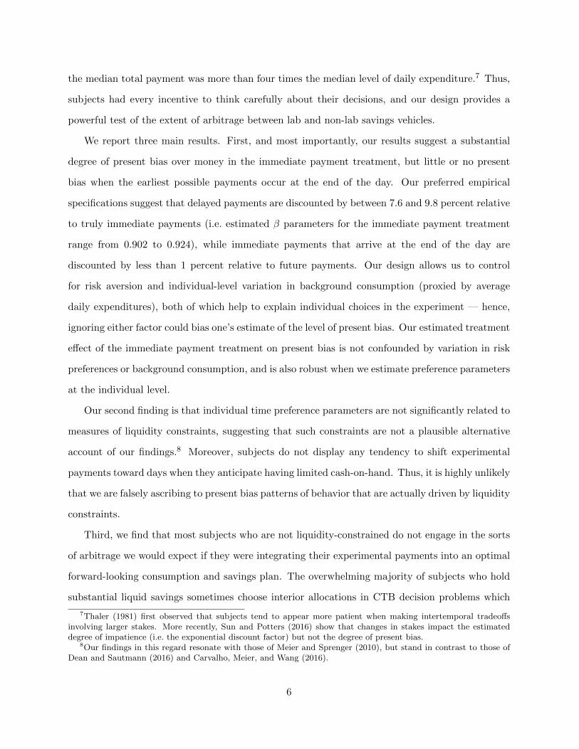
Next, we explore these patterns in a regression framework. We regress the budget fraction

allocated to the earlier payment date on an indicator for decisions where the front-end delay is

0, an indicator for the end-of-day payment treatment, and an interaction between the two. In all

specifications, we also include controls for the budget size, the interest rate, and the delay between

payments. We report OLS specifications as well as Tobit specifications that adjust for censoring

of the dependent variable at 0 and 1. Standard errors are clustered at the session level (Cameron

and Miller 2015).

Results are reported in Table 1. In all specifications, subjects allocate significantly more money

to the earlier payment date when the front-end delay is 0 — suggesting some degree of present

bias in the immediate payment treatment. Point estimates indicate that subjects allocated 2.9 to

4.3 percentage points more of their early-valued budgets to the earlier payment date when early

payments occurred immediately after the experiment (i.e. when the front-end delay was 0 in the

immediate payment treatment). Though the effect is relatively modest, it is significant at the 99

percent level in both the OLS and the Tobit specifications (p-values < 0.001).28

In contrast, we can never reject the hypothesis that allocation decisions do not depend on

the degree of front-end delay in the end-of-day payment treatments. The interaction between the

indicators for the end-of-day payment treatment and for decisions involving no front-end delay is

consistently negative and significant; this indicates that the treatment effect of the front-end delay

28As discussed above, the magnitude of this reduced form effect is comparable to that observed by Augenblick,Niederle, and Sprenger (2015). The standard errors reported in Column 1 of Table 1 indicate that we have a powerof 0.8 to detect an effect as small as 1.68 (Haushofer and Shapiro 2016).

18

of 0 is smaller in the end-of-day payment treatments than in the immediate payment treatments.

Tests of the overall impact of same-day payments on the allocation to the earlier payment date

consistently fail to reject the null for the end-of-day payment treatment (p-values 0.462 and 0.693).

Thus, our reduced form results suggest that delaying payments by a few hours all but eliminates

present bias.

4.3 Estimating the Degree of Present Bias

Next, we test for the presence of present bias by estimating β directly in a structural framework.

We estimate

c∗t =

{[β] δk(1 + r)

}−1/ρ(1 + r)m−

(1−

{[β] δk(1 + r)

}−1/ρ)ω

1 + {[β] δk(1 + r)}−1/ρ (1 + r)(8)

where, given an indicator for the end-of-day payment treatment, 1eod, and an indicator for decisions

with a the front-end delay of 0 days, 1t=0, we define

β = βimmediate × 1t=0 × (1− 1eod) + βeod × 1t=0 × 1eod + (1− 1t=0) ,

δ = δimmediate × (1− 1eod) + δeod × 1eod,

and

ρ = ρimmediate × (1− 1eod) + ρeod × 1eod.

We begin by estimating the β, δ, and ρ parameters via non-linear least squares (NLS).29 We report

three specifications which take different approaches to the background consumption parameter, ω.

First, we impose the assumption that subjects narrowly bracket their decisions in the experiment

by setting ω equal to 0. We then allow ω to vary across subjects by proxying for background

consumption with self-reported average daily expenditure, ωi. Finally, we estimate ω as one of the

model parameters. Results are reported in Table 2.

Though parameter estimates differ slightly across specifications, they paint a consistent picture.

29To facilitate comparisons of parameter magnitudes across treatment (without necessitating an unduly largenumber of digits), we report weekly discount factors throughout the analysis.

19

The estimated β parameters are significantly less than 1 in the immediate payment treatment,

indicating that subjects’ choices are present-biased. The estimates of β range from 0.902 to 0.924,

and all coefficients are significantly different from 1 at the 99 percent confidence level (all p-values

< 0.001). In the end-of-day payment treatment, we do not observe a statistically significant degree

of present bias. The estimates of β are higher, ranging from 0.982 to 0.992 — suggesting at most

an extremely modest amount of present bias when payments are made several hours after the

experimental session. In all specifications, we can reject the hypothesis that the degree of present

bias is equal in the immediate and end-of-day payment treatments (p-values range from 0.014 to

0.025 across specifications).

Turning to the estimated δ parameters, we find that subjects in both the immediate and the

end-of-day payment treatments are extremely impatient. Estimated weekly discount factors range

from 0.942 to 0.950 in the immediate payment treatment, versus 0.961 to 0.972 in the end-of-day

payment treatment. All are significantly different from 1 at at least the 95 percent confidence level.

These estimates suggest that payments 1 year in the future are discounted by between 77 and 96

percent. Though point estimates are higher in the end-of-day payment treatment, we can only

reject the hypothesis that δ is the same in the two treatments in 1 of 3 specifications (p-values

range from 0.050 to 0.132 across specifications).

The estimates of ρ and ω, in contrast, are broadly comparable in the immediate and end-of-day

payment sessions. The estimates of ρ are (unsurprisingly) higher in the specifications that allow

for positive background consumption (Columns 2 and 3 of Table 2), but do not differ substantially

across experimental treatments. Estimates suggest moderate risk aversion, with estimated values

of ρ between 0.5 and 1 in all specifications.30 Estimating the background consumption parameter,

ω, structurally and allowing it to vary across experimental treatments (in Column 3 of Table 2)

generates results that are quite similar to those obtained by using self-reported daily expenditures

as a measure of background consumption (in Column 2 of Table 2). This is reassuring since not

all estimation approaches allow for the direct estimation of ω.31 We do not find evidence that ω

30Though we take an entirely different approach to preference elicitation, our results are similar to estimates ofrisk aversion in broadly comparable field populations (cf. Harrison, Humphrey, and Verschoor 2010, Jakiela andOzier 2016).

31The estimation of ω also relies heavily on the functional form assumption regarding u(·). Using self-reporteddaily expenditures is preferable in that it simplifies estimation (since fewer parameters need to be estimated) and

20

differs significantly across treatments.

4.3.1 Robustness Checks

Alternative Approaches to Parameter Estimation. A weakness of the NLS approach is

that it does not adjust for censoring. This limitation could potentially bias parameter estimates

in our context because allocations were constrained to [0,m] for the earlier payment date and to

[0, (1+r)m] for the later payment date. In what follows, we report two alternative sets of parameter

estimates that address this issue. First, we estimate β, δ, and ρ parameters for each experimental

treatment via maximum likelihood. We assume an additively separable error term and let zin

denote subject i’s observed allocation to the earlier payment date in decision problem n:

zin = c∗t (mn, kn, rn, ωi|β, δ, ρ) + εin (9)

where c∗t is the optimal allocation to the earlier payment date, as defined by Equation 8, and εin

is a normally-distributed error term with mean 0 and variance σε.32 After adjusting for censoring

of c∗t at 0 and m, the log-likelihood function takes the standard form:

` (β, δ, ρ, σ) = ln

[1− Φ

(c∗tσε

)]× 1zin=0

+ ln

[φ

(c∗tσε

)/σε

]× (1− 1zin=0 − 1zin=mn)

+ ln

[1− Φ

(mn − c∗tσε

)]× 1zin=mn .

(10)

Results are reported in Table 3. We estimate two specifications: in Column 1, we set background

consumption to 0 for all subjects; in Column 2, we use self-reported daily expenditures, ωi.

We find no major differences between our maximum likelihood estimates of the model param-

eters and the NLS estimates reported above. Most importantly, our estimates of βimmediate are

significantly less than 1 in both specifications (p-values < 0.001), indicating a significant degree of

present bias in the immediate payment treatment. Our estimates of βeod are consistently higher

controls for potentially important variation in background consumption across subjects.32See Andersen, Harrison, Lau, and Rutstrom (2008), Choi, Kariv, Muller, and Silverman (2014), and Fisman,

Jakiela, and Kariv (2014) for related modeling approaches.

21

(though still less than 1), and we can never reject the hypothesis of no present bias in the end-of-

day payment treatment (p-values 0.207 and 0.246). We can reject the hypothesis that the degree

of present bias is equal across treatments (p-values 0.002 and 0.004).

As in our NLS specifications, we observe estimates of the δ parameters that are well below 1,

suggesting that subjects are quite impatient. Parameter estimates indicate that subjects in the

immediate payment treatment reveal an annual discount rate of approximately 99 percent, while

those in the end-of-day payment treatment reveal an annual discount rate of approximately 96

percent. We also observe moderate risk aversion in both experimental treatments.

Following Andreoni and Sprenger (2012a), we also consider an alternative estimation approach

to censoring: taking logs of the tangency condition characterizing the optimal interior solution.

When consumption utility takes the CRRA form, Equation 11 can be re-written as

c∗t + ω

c∗t+k + ω=[βδk(1 + r)

]−1/ρ; (11)

taking logs of both sides yields

ln

(c∗t + ω

c∗t+k + ω

)=

(−1

ρ

)lnβ +

(−1

ρ

)ln δ × k +

(−1

ρ

)ln (1 + r) (12)

which can be re-written as

ln

(c∗t + ω

c∗t+k + ω

)=

(−1

ρimmediate

)lnβimmediate × (1− 1eod)× 1t=0 +

(−1

ρeod

)lnβeod × 1eod × 1t=0

+

(−1

ρimmediate

)ln δimmediate × k × (1− 1eod) +

(−1

ρeod

)ln δeod × k × 1eod

+

(−1

ρimmediate

)ln (1 + r)× (1− 1eod) +

(−1

ρeod

)ln (1 + r)× 1eod.

(13)

We estimate Equation 13 via two-limit Tobit, adjusting for censoring of c∗t at 0 and m.33 Results

are reported in Table 4.

Tobit estimates are consistent with our earlier findings. Again, we find a significant degree of

33The key distinction between this approach and the maximum likelihood strategy described above is that weimplicitly assume a multiplicative (rather than an additive) error term in the latter.

22

present bias in the immediate payment treatment; again, estimated β parameters are higher —

and are not significantly less than 1 — in the end-of-day payment treatment (though, in the Tobit

specifications reported in Table 4, we cannot reject the hypothesis that the degree of present bias

is comparable across treatments). Our Tobit results differ from our NLS and ML estimates in

that the estimated β parameters are lower in the Tobit specifications, while the estimated δ and ρ

parameters are somewhat higher. Nonetheless, the overall pattern of findings remains unchanged:

we observe a statistically significant degree of present bias in the immediate payment treatment,

but not in the end-of-day payment treatment.

Sample Restrictions. As an additional robustness check, we replicate our NLS estimation in

sub-samples of subjects who showed high levels of comprehension and consistency: those subjects

who never violated GARP and those with basic consistency indices above 0.85 (i.e. those who

display a degree of adherence to the law of demand that is never observed among simulated subjects

who choose random points on each budget line). Results (which are reported in Online Appendix

Tables A3 and A4) are consistent with those observed in the unrestricted sample. Specifically, we

can always reject the hypothesis that βimmediate equals 1; the estimates of βeod are consistently

higher (though still typically less than 1), and we can never reject the hypothesis that βeod equals

1. We can also typically reject the hypothesis that βimmediate equals βeod.34 Thus, our results

are robust to the exclusion of those subjects who might have misunderstood the experiment; our

findings hold in a restricted sample of individuals who appear to make unambiguously rational and

consistent choices.

CARA Utility. To address concerns that our results might be driven by our assumption that

consumption utility takes the CRRA form, we also report NLS estimates of β and δ derived under

the assumption that utility takes the constant absolute risk aversion (CARA) form:

u(ct) = −e−αct . (14)

34Across the 6 specifications reported, the p-values associated with the hypothesis that βimmediate = βeod are 0.019,0.026, 0.029 (twice), 0.032, 0.045, and 0.115.

23

Under CARA utility, the optimal allocation to the earlier payment date is:

c∗t =1

(2 + r)

[ln(β)

−α+k ln(δ)

−α+

ln(1 + r)

−α+m(1 + r)

]. (15)

The optimal allocation to the earlier payment date does not depend on background consumption

when utility takes the CARA form, so we report only one set of results (in Table 5).

Our results are, again, consistent with our earlier findings: βimmediate is significantly less than

1 (p-value < 0.001), while βeod is significantly higher than βimmediate (p-value 0.038) and not

significantly less than 1 (p-value 0.542). The assumption of CARA utility also does not impact

our conclusion that subjects are fairly impatient, with estimated δ parameters well below 1. Thus,

our results appear to hold across specifications and functional form assumptions: choices in our

immediate payment treatment provide strong evidence of present bias over money, but present bias

appears to be attenuated substantially when payments occur at the end of the day.

4.4 Individual-Level Analysis

We next examine decisions in our experiment at the individual level. An advantage of our ex-

perimental design is that it allows us to estimate β and δ at the subject level without needing to

assume that the distribution of individual-level parameters takes a specific functional form.35 We

estimate subject-level βi, δi, and ρi parameters via non-linear least squares while controlling for

self-reported background consumption (average daily expenditure).36

CDFs of the estimated individual-level βi, δi, and ρi parameters are presented in Figure 4.37 The

35In other words, our functional form assumptions impose restrictions on individual preferences (most notably, weassume that discounting is either quasi-hyperbolic or exponential), but we impose no restrictions on the relationshipbetween individual preference parameters (across subjects). See Choi, Fisman, Gale, and Kariv (2007a), Fisman,Kariv, and Markovits (2007), Choi, Kariv, Muller, and Silverman (2014), and Fisman, Jakiela, and Kariv (2014) forexamples of similar estimation approaches that estimate preference parameters at the individual level. This approachcontrasts with the estimation strategies used in Andersen, Harrison, Lau, and Rutstrom (2008), Von Gaudecker, vanSoest, and Wengstrom (2011), and Jakiela and Ozier (2016), who estimate mixed logit models of individual choices.

36We are unable to estimate individual parameters for 17 of our 494 subjects. 6 subjects always allocated theirentire endowment to the earlier payment date, and 9 always allocated their entire endowment to the later paymentdate. Estimation does not converge for 2 of the remaining subjects.

37Like other recent studies of individual preferences (cf. Choi, Fisman, Gale, and Kariv 2007a, Fisman, Kariv,and Markovits 2007, Andersen, Harrison, Lau, and Rutstrom 2008, Fisman, Jakiela, and Kariv 2014), we observetremendous individual heterogeneity in preferences, much of which is not explained by demographic and socioeco-nomic characteristics. The 5th percentile of βi is 0.164, and the 95th percentile is 1.598. The 5th percentile of δi is0.473, and the 95th percentile is 1.388. The 5th percentile of ρi is 0.243, and the 95th percentile is 17.878.

24

distribution of individual-level βi parameters in the immediate payment treatment is consistently

to the left of the distribution the end-of-day payment treatment, suggesting greater present bias

when payments are truly immediate. Indeed, the median individual-level βi in the immediate

payment treatment is 0.938, versus 0.978 in the end-of-day payment treatment, and we can reject

the hypothesis that the medians are equal in the two treatments (p-value 0.059). 61 percent of

subjects in the immediate payment treatment have estimated βi parameters below 1, versus 55

percent of those in the end-of-day payment treatment.38,39 Thus, subjects who show some degree

of present bias outnumber those who tend toward future bias by a wide margin, though present

bias is far from universal.40

Panel A of Figure 5 compares the proportion of subjects displaying a statistically significant

degree of present bias across treatments.41 26 percent of subjects assigned to the immediate

payment treatment have estimated βi parameters that are significantly less than 1, versus 17

percent of subjects assigned to the end-of-day payment treatment. In contrast, only 8 percent of

subjects assigned to the immediate payment treatment and 9 percent of those assigned to the end-

of-day payment treatment are future-biased (in the sense of having βi significantly greater than 1).

Thus, (statistically significant) present bias is more common than (statistically significant) future

bias — suggesting that the former does not only result from subjects’ tendency to implement their

choices with error — and it is more common in the immediate payment treatment than in the

end-of-day payment treatment.42

Next, we examine our estimated δi parameters. We observe considerable variation in patience,

38We cannot reject the hypothesis that the proportion of subjects with estimated βi parameters below 1 is equalin the immediate and end-of-day payment treatments (p-value 0.211).

39For comparison, when Augenblick, Niederle, and Sprenger (2015) estimate individual level βi parameters usingdata from effort choices, they find that 56 percent of subjects have estimated βi parameters below 0.99. Whenparameters are estimated using data from CTB decisions over money payments, only 33 percent of subjects haveestimated βi parameters below 0.99.

40Moreover, as the CDF presented in Figure 4 makes clear, the distribution of βi is smooth and steep in theneighborhood of 1 in both treatments; thus, quite a few subjects have estimated βi parameters that suggest anextremely weak tendency toward either present or future bias.

41We classify a subject as displaying a significant degree of present (resp. future) bias if βi is less (resp. greater)than 1 and we can reject the hypothesis that βi equals 1 at the 90 percent confidence level. Since subjects madeonly 48 CTB decisions, these individual-level statistical tests are, to some extent, under-powered — we may fail toreject the hypothesis that βi equals 1 when subjects implement their (present-biased or future-biased) preferenceswith error.

42We can reject the hypothesis that the likelihood of displaying a statistically significant degree of present bias iscomparable across treatments (p-value 0.030), but we cannot reject the hypothesis that the likelihood of displayinga significant degree of future bias is the same in the immediate and end-of-day payment treatments (p-value 0.724).

25

though — as the aggregate estimates suggest — most subjects tend to discount the future sharply.

The median δi in the immediate payment treatment is 0.938, versus 0.958 in the end-of-day pay-

ment treatment.43 These weekly discount factors suggest that subjects in the immediate payment

treatment discount payments 1 year in the future by 96 percent, versus 89 percent for the end-

of-day payment treatment. Though the CDFs presented in Panel B of Figure 4 do not suggest a

consistent difference in δi across treatments, Panel B of Figure 5 shows that subjects are somewhat

more likely to display a statistically significant degree of impatience in the immediate payment

treatment.44 Our results also suggest that present bias and impatience are positively correlated

(Spearman’s ρ = 0.176).45

To further test whether delaying experimental payments attenuates present bias, we report

OLS regressions of the estimated individual-level βi, δi, and ρi parameters on an indicator for

the end-of-day payment treatment (Table 6). When no controls are included, coefficient estimates

suggest that βi is significantly higher in the immediate payment treatment than in the end-of-day

payment treatment (p-value 0.044).46 In contrast, assignment to the end-of-day payment treatment

does not impact patience (δi) or risk aversion (ρi).47 Results are similar when we include controls

for individual characteristics such as age, gender, and education level (in Columns 4 through 6 of

Table 6). Thus, though we observe substantial heterogeneity in individual preference parameters,

our individual-level analysis confirms the main conclusion of our aggregate analysis: present bias

is reduced when payments are not made immediately after the experimental session.

43We can just reject the hypothesis that the medians are equal in the two treatments (p-value 0.090).4447 percent of subjects in the immediate payment treatment have estimated δi parameters that are significantly

less than 1, versus 40 percent in the end-of-day payment treatment. We also find that 10 percent of subjects in theimmediate payment treatment have estimated δi parameters that are significantly greater than 1, versus 14 percentin the end-of-day payment treatment. We cannot reject the hypothesis that the probability of having a δi that issignificantly below 1 is equal across treatments (p-value 0.139); nor can we reject the hypothesis that having a δisignificantly above 1 is equal across treatments (p-value 0.170).

45We also observe substantial heterogeneity in risk aversion, though — as the CDFs present in Panel C of Figure4 indicate — this does not differ across treatments. The median individual-level CRRA coefficient is 0.935 in theimmediate payment treatment, versus 0.941 in the end-of-day payment treatment. We cannot reject the hypothesisthat the median ρi is the same in the immediate and end-of-day payment treatments (p-value 0.897).

46We can reject the hypothesis that the average individual-level βi parameter in the immediate payment treatment(i.e. the constant in the OLS regression reported in Column 1 of Table 6) is equal to 1 (p-value < 0.001). We cannotreject the hypothesis that the average individual-level βi parameter in the end-of-day payment treatment is equal to1 (p-value 0.389).

47We can reject the hypothesis that the mean δi parameter is equal to 1 for both the immediate and the end-of-daypayment treatments (p-values < 0.001).

26

5 Discussion

Over the last few years, several theoretically sophisticated, technically rigorous experiments have

sparked a lively debate about the use of lab experimental methods to measure intertemporal

tradeoffs (cf. Andreoni and Sprenger 2012a, Augenblick, Niederle, and Sprenger 2015, Dean and

Sautmann 2016, Halevy 2015, Epper 2015, Carvalho, Meier, and Wang 2016, Gine, Goldberg, Sil-

verman, and Yang 2017, Janssens, Kramer, and Swart 2017). This body of work raises two critical

questions. First, do lab experiments with money payments measure time preferences? Utility

is defined over consumption, not money, and subjects have access to a range of credit products.

So, sophisticated subjects may treat dated experimental payments as a(nother) form of credit,

integrating their (present-discounted) experimental income into an optimal forward-looking con-

sumption plan — in which case, choices in the lab will reflect market interest rates and (perhaps)

individual liquidity constraints, but not individual preferences (Coller and Williams 1999, Dean

and Sautmann 2016, Carvalho, Meier, and Wang 2016). Second, even if one assumes that trade-

offs in experiments with money payments are driven by time preferences, should static preference

reversals be interpreted as evidence of present bias? As discussed at length in Halevy (2015) and

Gine, Goldberg, Silverman, and Yang (2017), this interpretation assumes that subjects have sta-

ble utility functions and discount rates — that one’s willingness to make tradeoffs between dated

payments that arrive 1, 2, or 3 (or 100, 200, or 300) days from “now” does not depend on the

calendar date upon which one is asked. Of course, the assumption that preferences are stable is

standard in economics; however, even subjects with stable preferences may seek to shift money

toward points in time when they expect the marginal utility of money to be high (because, for

example, they anticipate needing to make a large payment or being short of income), particularly

if credit markets are imperfect.48

48Stigler and Becker (1977) argue that economists should not accept heterogeneity in preferences (“tastes”) asan explanation for differences in choice behavior across individuals or periods; instead, they suggest that humanbeings are homogeneous, and that economists should seek price and income based explanations for differences inbehavior. However, the hypothesis that individual preferences are heterogeneous (across individuals) has now beenconfirmed in a large number of controlled lab experiments (cf. Andreoni and Miller 2002, Choi, Fisman, Gale, andKariv 2007a, Fisman, Kariv, and Markovits 2007, Andersen, Harrison, Lau, and Rutstrom 2008, Von Gaudecker, vanSoest, and Wengstrom 2011, Choi, Kariv, Muller, and Silverman 2014, Fisman, Jakiela, and Kariv 2014). Whetherfuture work will also rule out the hypothesis that preferences are stable over time — at least after one properlycontrols for variation in income, prices, and other arguments that enter into the utility function — remains to be seen;however, we take this assumption as a natural point of departure for economic research, and focus on explanations

27

Providing definitive answers to these questions is beyond the scope of this paper. However, our

experiment does allow for explicit tests of a number of the hypotheses under scrutiny. Moreover, it

is incumbent upon us to show that phenomena other than present bias cannot explain the observed

tendency to shift money toward immediate payments. In what follows, we compare our results to

those of other recent studies and present several additional pieces of analysis that speak to these

questions. First, we test whether subjects behave in the manner predicted by standard models of

intertemporal optimization, exploiting the high interest rates offered through the experiment to

increase their present-discounted income stream. Second, we test whether subjects shift experimen-

tal payments toward dates when they expect to have limited liquidity. After presenting evidence

against these alternative explanations for our main results, we examine our structural estimates of

time preference parameters and discuss their policy implications.

5.1 Do Subjects Engage in Arbitrage?

Economists typically assume that people have access to perfect credit markets, and that their

intertemporal tradeoffs are part of an optimal forward-looking consumption plan characterized by

a set of Euler equations. However, most experimental economists — including those using lab

experimental methods to study discounting — assume that subjects engage in narrow bracketing,

viewing their dated lab experimental payments in isolation, as though they were consumption plans

(Andersen, Harrison, Lau, and Rutstrom 2008, Rabin and Weizsacker 2009). Coller and Williams

(1999) were some of the first to question this assumption, highlighting the fact that experimental

subjects with access to credit should engage in arbitrage, choosing immediate payments when the

gross interest rate within the experiment is lower than their return on savings, and choosing delayed

payments when the experimental return is lower than their cost of borrowing. More recently, Dean

and Sautmann (2016) provide evidence that the intertemporal tradeoffs made by subjects in their

(lab-in-the-field) experiment are related to liquidity constraints and accumulated savings outside

of the lab — suggesting that the narrow bracketing assumption fails in their data. Building on

Harris and Laibson (2001), Dean and Sautmann (2016) propose a model in which sophisticated,

for variation in revealed preferences (within individual over time) that are related to predictable variation in incomeand anticipated expenditures.

28

potentially credit-constrained consumers make optimal forward-looking plans that integrate their

experimental payments into their consumption streams. If the assumptions of their model hold,

then lab experiments cannot be used to measure individual time preferences; instead, they measure

marginal rates of substitution across periods, which depend on market interest rates and subjects’

anticipated income and expenditures in all future periods.49

CTB experiments allow for explicit tests of the extent to which subjects engage in these

types of arbitrage between lab and non-lab savings vehicles (Gine, Goldberg, Silverman, and

Yang 2017): because (many of) the implicit interest rates offered in experiments are typically

well above those available through the credit market, subjects who integrate lab payments into

fully-optimal forward-looking consumption plans should only choose immediate consumption if

they are liquidity-constrained; those who hold liquid savings should allocate their entire endow-

ment to the later payment date when the (implicit) lab interest rate exceeds the return on their

savings (because this maximizes the net present value of their income stream).50

We test this prediction in our data by dividing the sample into subjects known to have liquid

savings in excess of the maximum early payment (the 28 percent of subjects who have more than

1,000 Kenyan shillings, or 10.20 USD, in a savings account) and those who might be liquidity-

constrained (those who do not have 1,000 Kenyan shillings in a savings account). Figure 6 plots

the proportion of subjects within each category who always allocate their entire endowment to

the later payment date. The figure makes it clear that, though corner solutions are common,

those subjects who are not liquidity-constrained do not appear to be engaging in arbitrage by

consistently cashing in on the extremely high interest rates offered in the experiment. Across all

49Of course, it is entirely possible that both of these extreme modeling assumptions — narrow bracketing with 0background consumption and full dynamic optimization — fail to provide a psychologically realistic description ofthe ways human beings actually make financial decisions (both inside and outside the lab). If savings are illiquid orthere are substantial transaction costs to borrowing or lending, people are unlikely to engage in the types of arbitrageproposed by Coller and Williams (1999), and the tradeoffs made in the lab (over moderate amounts of money) arelikely to have little to do with the market interest rate. The same may be true if there are large cognitive costs informing an optimal forward-looking consumption and savings plan (or re-optimizing in response to a moderately-sizedshock). Moreover, even outside the lab, there is ample evidence that people do not smooth moderately-sized one-offpayments over their lifetimes (cf. Halevy 2014).

50In addition, those who can borrow at an interest rate below that offered by the experiment should also allocatetheir entire endowment to the later payment date. However, it is difficult to collect reliable information on subjects’access to credit (and the interest rates that they would face) outside of the lab — particularly if borrowing wouldtake place outside of the formal credit market. We therefore focus on the subset of subjects who hold moderateamounts of money in savings accounts since it is apparent that these individual are not liquidity-constrained.

29

interest rates, only 2.6 percent of subjects with liquid savings in the bank always allocate their

entire endowment to the later payment date, versus 1.7 percent of those without 1,000 shillings in

the bank.51 Focusing on extremely high gross interest rates of at least 2 (i.e. guaranteed returns of

at least 100 percent over a 2 to 4 week time horizon), which are very unlikely to be available outside

the lab, we find that 13.8 percent of those who are not liquidity-constrained always allocate the

entire endowment to the later payment date, versus 7.8 percent of those without 1,000 shillings in

the bank. We can reject that the proportion of subjects engaging in such behavior is equal across

groups (those who are not liquidity-constrained versus those who may be liquidity-constrained).

Nonetheless, our data make it clear that most subjects are not engaging in the types of arbitrage

that we would expect if lab payments were integrated into an optimal forward-looking consumption

and savings plan.52,53,54,55

The results presented above demonstrate that most subjects who are not liquidity-constrained

make choices that appear to reflect their preferences rather than their arbitrage opportunities. A re-

lated question is whether our main finding (of present bias when payments are truly immediate, but

not when payments occur at the end of the day) might be explained by liquidity constraints, which

could cause (liquidity-constrained) subjects to take immediate payments whenever possible. If our

results were driven by liquidity constraints, we would expect our indicator of liquidity constraints

to be correlated with the estimated individual-level βi parameter. However, the individual-level

51We cannot reject the hypothesis that the proportions of not liquidity-constrained and potentially liquidity-constrained subjects are equal (p-value 0.523).

52Across all subjects, only 1.8 percent always allocate their entire endowment to the later payment date, and only8.9 percent always do so at the higher interest rates.

53Interestingly, our results differ from those of Andreoni and Sprenger (2012a) in this regard: 70 percent of theCTB decisions observed in their experiment are corner solutions, suggesting that arbitrage may be a more reasonableexplanation of behavior in that context. In our experiment, subjects who are not liquidity-constrained choose cornersolutions 46.5 percent of the time; those who are potentially liquidity-constrained choose corner solutions 38.5 percentof the time.

54One possible concern with this test is that subjects might choose allocations near the middle of the choice set forreasons that are not related to intertemporal preferences. Though we cannot entirely rule out this possibility, it isunlikely to explain our main results (on the difference in present bias across experimental treatments). Any tendencyto choose points near the middle of the choice set would impact the estimated level of risk aversion, but shouldnot have differential impacts on time preferences across treatments. Importantly, we do not observe an associationbetween assignment to the end-of-day payment treatment and our individual-level measure of risk aversion (ρi), soany tendency to choose allocations near the center of the choice set does not differ across treatments and cannotexplain the effect of the immediate payment treatment on present bias.

55We cannot reject the hypothesis that the proportion of subjects who always allocate their entire endowmentto the later payment date is equal across treatments (p-value 0.941), nor can we reject the hypothesis that theproportion of subjects who always allocate their entire endowment to the later payment date when the interest rateis at least 2 is equal across treatments (p-value 0.956).

30

regressions presented in Table 6 do not suggest that this is the case: the point estimate associated

with the indicator for having at least 1,000 Kenyan shillings in a liquid savings account is close

to 0 and not statistically significant.56 Moreover, it is not clear why liquidity constraints would

have a differential impact on allocation decisions that depends on the timing of the experimental

payments within the space of a few hours (i.e. whether payments arrive immediately after the

experimental session and not at the end of the day).57 Thus, neither liquidity constraints nor

arbitrage opportunities can explain our overall pattern of results.

5.2 Real and Perceived Changes in Background Consumption

A more general mis-specification concern, suggested by Halevy (2015), is that consumption utility

may not be stable over time. Though our main finding (the existence of present bias over money

when payments are immediate) is robust to a range of assumptions about the background con-

sumption parameter (ωi), our estimates of the magnitude of the present bias parameter (βi) vary

across specifications. Moreover, we have assumed that background consumption does not vary

across payment dates. If background consumption is systematically higher in the future relative to

the present (for example, because of optimism or overconfidence), subjects might appear present-

biased when in fact they are not. Alternatively, if background consumption reflects beliefs about

future cash flow or liquidity (which might vary across payment dates), choice patterns that appear

present-biased might result from subjects’ attempts to shift payments toward dates when they

anticipate that the marginal utility of consumption will be higher (for example, because they will

have relatively little income or cash on hand), as suggested by Dean and Sautmann (2016), Halevy

(2015), and Ambrus, Asgeirsdottir, Noor, and Sandor (2015). If subjects are shifting payments

toward days when they expect the marginal utility of income to be high (because of actual or

56This finding is in line with earlier work by Meier and Sprenger (2010): in a sample of low-income tax-filers in theU.S., they find that “time preference measures are generally uncorrelated with credit constraints, future liquidity, orcredit experience. This indicates that differential credit access, liquidity, and experience are unlikely to be drivers ofexperimental responses, and cannot explain the observed heterogeneity of present bias” (Meier and Sprenger 2010,pp. 202–203). In contrast, Carvalho, Meier, and Wang (2016) and Dean and Sautmann (2016) present evidence thatliquidity constraints may explain the observed tendency toward present observed in their experimental data. Recentwork by Ambrus, Asgeirsdottir, Noor, and Sandor (2015) shows that individuals with incomes that are stable overtime do not display present bias over money.

57Interestingly, subjects assigned to the immediate payment treatment are somewhat less likely to be liquidity-constrained than those assigned to the end-of-day payment treatment. If our results were driven by expectations ofliquidity constraints, we would expect precisely the opposite.

31

perceived variation in ωi over time, static preferences reversals may or may not constitute evidence

of dynamic inconsistency (Halevy 2015).

We present two pieces of evidence that our results are not driven by intertemporal variation in

background consumption or the perceived marginal utility of income. First, we expand our main

NLS specification to allow background consumption to differ between the earlier and later payment

dates. This would, for example, capture any optimism about future income streams relative to the

present. For each treatment, we estimate separate parameters ωearliertreatment and ωlatertreatment.58 Results

are reported in Table 7. Importantly, allowing background consumption to differ across earlier

vs. later payment dates does not impact our main result: we still observe present bias in the

immediate payment treatment but not in the end-of-day payment treatment, and we can still

reject the hypothesis that the degree of present bias is equal across treatments. Turning to the

estimated background consumption parameters, we can never reject the hypothesis that background

consumption is equal across treatments. However, we do find some qualified support for differences

in background consumption across payment dates. The estimated level of background consumption

is higher at the later payment date in both treatments, though the (within-treatment) difference

is only significant in the immediate payment treatment. This suggests that optimism about future

income may play some role in intertemporal choices, but controlling for it does not eliminate present

bias.

To further explore this issue, we added a series of questions about anticipated liquidity to

the post-experiment survey. For each of the five possible payment dates in the experiment, we

asked subjects whether they expected to have more cash-on-hand than normal, less than normal,

or approximately the typical amount. These questions were only administered during the last

20 experimental sessions, so we have data from 324 of our 494 subjects. We observe substantial

within-subject variation in anticipated liquidity: only 31.2 percent of subjects showed no variation

in expected cash-on-hand across payment dates. As a result, we can use this self-reported measure

of expected liquidity to test whether subjects shift income from the experiment toward dates when

they expect to have relatively little cash-on-hand.

In Table 8, we replicate the reduced form regressions reported in Table 1 in the sample of

58We therefore estimate four parameters: ωearlierimmediate, ωlater

immediate, ωearliereod , and ωlater

eod .

32

subjects who answered our liquidity questions, regressing the fraction of the endowment allocated

to the earlier payment date on an indicator for having a front-end delay of 0 days, an indicator

for the end-of-day treatment, an interaction between the two, and controls for the delay between

payments, the interest rate, and the endowment size. As expected, results are similar to those

in the full sample (Table 8, Columns 1 and 4). In Columns 2 and 5, we add an indicator for

having lower expected liquidity (cash-on-hand) at the later payment date, relative to the earlier

payment date. If subjects were shifting their experimental payments toward periods of anticipated

low liquidity, then the coefficient on our difference-in-liquidity variable should be negative and

significant (because subjects will allocate less to the earlier payment date when they anticipate

having lower background consumption on the later payment date). In fact, we find the opposite:

the coefficient on our difference-in-liquidity variable is positive and significant (Table 8, Columns

2 and 5). Moreover, including this variable has no impact on our main result: we continue to

observe present bias in the immediate payment treatment (i.e. the amount allocated to the earlier

payment date is higher when the front end delay is 0 days in the immediate payment treatment),

and we do not observe present bias in the end-of-day payment treatment. Results are similar when

we interact our difference-in-liquidity variable with the indicator for assignment to the end-of-day

payment treatment (Table 8, Columns 3 and 6). Thus, we find no evidence that subjects reduce

their allocation to the earlier payment date when they expect marginal utility to be higher at the

later payment date, and we can rule out the possibility that such predictable changes in marginal

utility explain our main results.

5.3 Parameter Magnitudes and Policy Implications

In our final piece of analysis, we discuss the implications of our results for policy. Our results suggest

a statistically significant level of present bias over money when payments are truly immediate.

An important question is whether the degree of present bias that we observe is economically

significant. Our parameter estimates also suggest lower levels of patience in the immediate payment

treatment than in the end-of-day payment treatment, though the difference between treatments is

only statistically significant in some specifications.

In Figure 7, we illustrate the minimum per-period return that would induce subjects with

33

preference parameters consistent with our NLS estimates (from Column 1 of Table 2) to make

investments, comparing the results of our immediate payment and end-of-day payment treatments.

The figure highlights several important implications of our results. First, though our structural

estimate of β in the immediate payment treatment (0.902) is not unusually low, it has a dramatic

impact on the willingness to make short-term investments: a subject with β = 0.902, δ = 0.950,

ρ = 0.581, and ω = 0 would like to commit her future self to invest whenever the per-period

return exceeds 13 percent, but in reality she is only willing to invest today in a project that yields

a return of 45 percent next week. Moreover, the difference in the estimated β and δ parameters

across treatments leads to large differences in the willingness to make short-term investments; in the

short-term, most of this difference is explained by the higher estimated level of present bias in the

immediate payment treatment. This suggests that policy instruments that introduce extremely

short delays between decisions and “immediate” costs can lead to large increases in investment

levels — increases that could increase long-run welfare.59

For longer-term investments, of course, the impact of present bias is much less important:

when considering investments that yield benefits 1 year from now, present bias raises the minimum

required return by less than 1 percentage point.60 This highlights the second conclusion suggested

in the figure: the differences in estimated δ parameters appear at least as important, in terms

of explaining the low willingness to make long-term investments, as the differences in the present

bias across treatments (though they are less precisely estimated). As discussed above, our results

suggest that subjects are quite impatient, and we find suggestive evidence of greater impatience in

the immediate payment treatment than in the end-of-day payment treatment. When considering

investment horizons of a month or a year, the differences in patience translate into large differences

in the willingness to invest in the future. From a policy perspective, the key distinction between

investment decisions driven by present bias and those driven by impatience are that low levels of

investment explained by δ are unambiguously optimal from the perspective of individual welfare.

Our results suggest that those who appear present-biased may also be quite impatient, so low

59See O’Donoghue and Rabin (1999) for discussion of the difficulties of characterizing welfare when preferences arenot dynamically consistent. We use the term “long-run welfare” in the sense of the long-run welfare criterion thatthey propose.

60Though present-biased agents may put off making long-term investments when they (erroneously) expect toinvest tomorrow.

34

observed willingness to invest may or may not be suboptimal from a welfare perspective. It is

therefore critical that policymakers determine which structural parameters are driving investment

decisions within a particular context before designing policy instruments, since interventions that

increase investments may reduce welfare when low investment levels result from impatience rather

than present bias. Moreover, the fact that small differences in payment timing appear to generate

large differences in the willingness to invest (including economically meaningful differences in δ)

suggests that structural estimates of time preference parameters should be used with caution.

6 Conclusion

We conducted convex time budget experiments with truly immediate repayment to test whether

small delays of less than a day attenuate present bias. We exploited Kenya’s mobile money technol-

ogy M-Pesa to equalize transaction costs and uncertainty across all payment times and dates; we

also introduced experimental variation in whether same-day payments were available immediately

after the experiment or at the end of the day.

We find substantial evidence of present bias over money, but only when payments are truly

immediate. Parameter estimates suggest that all delayed payments are discounted by between

7.6 and 9.8 percent in our immediate payment treatments. In sessions where the earliest possible

payments arrive at the end of the day, we do not observe a statistically significant level of present

bias (and we can formally reject the hypothesis that the degree of present bias is the same in

both treatments). We also observe substantial heterogeneity in time preferences across subjects.

However, variables associated with likely liquidity constraints (or the lack thereof) do not predict

individual-level time preference parameters.

Our results — and, in our view, the results of many of the related studies listed above — point

to a few broad conclusions. First, neither the standard model of intertemporal tradeoffs (in which

lab payments are integrated into an optimal forward-looking consumption and savings plan) nor

the simplest form of narrow bracketing (with background consumption equal to 0) provides an

adequate description of the ways subjects make intertemporal tradeoffs in the lab. This suggests

that researchers should devote greater attention to the development of experiments explicitly de-

35

signed to test potential refinements of existing models, in order to build a more accurate positive

description of the decision-making process.61 Experiments intended to better understand the way

humans use mental accounting and heuristics to simplify the process of organizing their financial

lives seem likely to be particularly fruitful.

Second, our results suggest that (at least in some populations) present bias over money is

important when the earliest payments are truly immediate; our findings are consistent with models

such as the quasi-hyperbolic model (Laibson 1997, O’Donoghue and Rabin 1999) that predict a

sharp distinction between immediate and slightly delayed payments. However, our experiment is

not intended to trace out the relationship between individual discount factors and the level of the

front-end delay over the minutes and hours after decisions are made. As such, we are unable to

fully distinguish between the quasi-hyperbolic model and alternatives that do not suggest a clear

discontinuity between immediate and nearly immediate payments (cf. Kirby 1997). We leave that

to future work. It is also important to note that some other experiments involving immediate

payments — most notably, Augenblick, Niederle, and Sprenger (2015) — find little evidence of

present bias over money in university student samples. The differences between these findings and

our work suggest that some socioeconomic groups may be more prone to arbitraging between lab

and non-lab savings vehicles.

The development of the quasi-hyperbolic model of time preferences was motivated by the desire

to provide a better positive explanation of the ways humans actually make intertemporal tradeoffs.

However, since the advent of this tractable model of present bias, much of the energy has shifted

toward exploring its predictions in field settings and testing between the quasi-hyperbolic model

and the standard model. The new wave of theoretically-motivated time preference experiments,

and the controversies generated by the conflicting results of these studies, highlights the need for

more experimental work directed towards testing and refining the behavioral economic model of

intertemporal decisionmaking, with a specific focus on not only the extent of present bias, but the

ways subjects do or do not integrate controlled choices in the lab — or isolated decisions outside

of the lab — into a larger, long-term optimization problem. Such an integrated framework has

the potential to allow for a more complete reconciliation of existing results, and will also help

61Ambrus, Asgeirsdottir, Noor, and Sandor (2015) is an excellent example of work in this vein.

36

policymakers seeking to nudge citizens and consumers toward achieving their long-term savings

and consumption goals.

37

References

Acland, D., and M. R. Levy (2015): “Naivete, Projection Bias, and Habit Formation in Gym Atten-dance,” Management Science, 61(1), 146–160.

Afriat, S. N. (1967): “The Construction of Utility Functions from Expenditure Data,” InternationalEconomic Review, 8(1), 67–77.

Ainslie, G. (1975): “Specious Reward: A Behavioral Theory of Impulsiveness and Impulse Control,”Psychological Bulletin, 82(4), 463–496.

Ambrus, A., T. L. Asgeirsdottir, J. Noor, and L. Sandor (2015): “Compensated Discount Func-tions: An Experiment on the Influence of Expected Income on Time Preference,” .

Andersen, S., G. W. Harrison, M. I. Lau, and E. E. Rutstrom (2008): “Eliciting Risk and TimePreferences,” Econometrica, 76(3), 583–618.

Andreoni, J., B. Gillen, and W. Harbaugh (2013): “The Power of Revealed Preference Tests: Ex-PostEvaluation of Experimental Design,” working paper.

Andreoni, J., and J. Miller (2002): “Giving According to GARP: An Experimental Test of the Consis-tency of Preferences for Altruism,” Econometrica, 70(2), 737–753.

Andreoni, J., and C. Sprenger (2012a): “Estimating Time Preferences from Convex Budgets,” Ameri-can Economic Review, 102(7), 3333–56.

(2012b): “Risk Preferences Are Not Time Preferences,” American Economic Review, 102(7), 3357–3376.

Augenblick, N., M. Niederle, and C. Sprenger (2015): “Working Over Time: Dynamic Inconsistencyin Real Effort Tasks,” Quarterly Journal of Economics, 130(3), 1067–1115.

Becker, G. S. (1962): “Irrational Behavior and Economic Theory,” Journal of Political Economy, 70(1),1–13.

Bronars, S. G. (1987): “The Power of Nonparametric Tests of Preference Maximization,” Econometrica:Journal of the Econometric Society, 55(3), 693–698.

Cameron, C., and D. Miller (2015): “A Practitioner’s Guide to Cluster-Robust Inference,” Journal ofHuman Resources, 50(2), 317–372.

Carvalho, L. S., S. Meier, and S. W. Wang (2016): “Poverty and Economic Decision-Making: Evidencefrom Changes in Financial Resources at Payday,” American Economic Review, 106(2), 260–284.

Choi, S., R. Fisman, D. Gale, and S. Kariv (2007a): “Consistency and Heterogeneity of IndividualBehavior under Uncertainty,” American Economic Review, 97(5), 1921–1938.

(2007b): “Revealing Preferences Graphically: An Old Method Gets a New Toolkit,” AmericanEconomic Review, 97(2), 153–158.

Choi, S., S. Kariv, W. Muller, and D. Silverman (2014): “Who Is (More) Rational?,” AmericanEconomic Review, 104(6), 1518–1550.

Coller, M., and M. Williams (1999): “Eliciting Individual Discount Rates,” Experimental Economics,2(2), 107–127.

Dean, M., and A. Sautmann (2016): “Credit Constraints and the Measurement of Time Preferences,”working paper.

DellaVigna, S., and U. Malmendier (2006): “Paying Not to Go to the Gym,” American EconomicReview, pp. 694–719.

38

Epper, T. (2015): “Income Expectations, Limited Liquidity, and Anomalies in Intertemporal Choice,”Universitat st. gallen discussion paper 2015-19.

Fischbacher, U. (2007): “z-Tree: Zurich Toolbox for Ready-made Economic Experiments,” ExperimentalEconomics, 10(2), 171–178.

Fisher, I. (1930): The Theory of Interest. Augustus M. Kelley Publishers.

Fisman, R., P. Jakiela, and S. Kariv (2014): “The Distributional Preferences of Americans,” Nationalbureau of economic research working paper no. 20145.

Fisman, R., P. Jakiela, S. Kariv, and D. Markovits (2015): “The Distributional Preferences of anElite,” Science, 349(5254), aab0096.

Fisman, R., S. Kariv, and D. Markovits (2007): “Individual Preferences for Giving,” American Eco-nomic Review, 97(5), 1858–1876.

Frederick, S., G. Loewenstein, and T. O’Donoghue (2002): “Time Discounting and Time Preference:A Critical Review,” Journal of Economic Literature, pp. 351–401.

Gabaix, X., and D. Laibson (2017): “Myopia and Discounting,” National bureau of economic researchworking paper no. 23254.

Gine, X., J. Goldberg, D. Silverman, and D. Yang (2017): “Revising Commitments: Field Evidenceon the Adjustment of Prior Choices,” Economic Journal, doi:10.1111/ecoj.12378.

Halevy, Y. (2008): “Strotz Meets Allais: Diminishing Impatience and the Certainty Effect,” AmericanEconomic Review, 98(3), 1145–1162.

(2014): “Some Comments on the Use of Monetary and Primary Rewards in the Measurement ofTime Preferences,” working paper.

(2015): “Time Consistency: Stationarity and Time Invariance,” Econometrica, 83(1), 335–352.

Harris, C., and D. Laibson (2001): “Dynamic Choices of Hyperbolic Consumers,” Econometrica, 69(4),935–957.

Harrison, G. W., S. J. Humphrey, and A. Verschoor (2010): “Choice under Uncertainty: Evidencefrom Ethiopia, India and Uganda,” Economic Journal, 120(543), 80–104.

Haushofer, J. (2014): “The Cost of Keeping Track,” working paper.

Haushofer, J., and J. Shapiro (2016): “The Short-Term Impact of Unconditional Cash Transfers to thePoor: Experimental Evidence from Kenya,” Quarterly Journal of Economics, 131(4), 1973–2042.

Jakiela, P., and O. Ozier (2016): “Does Africa Need a Rotten Kin Theorem? Experimental Evidencefrom Village Economies,” Review of Economic Studies, 83(1), 231–268.

Janssens, W., B. Kramer, and L. Swart (2017): “Be Patient when Measuring Hyperbolic Discounting:Stationarity, Time Consistency and Time Invariance in a Field Experiment,” Journal of DevelopmentEconomics, 126, 77–90.

Kirby, K. N. (1997): “Bidding on the Future: Evidence Against Normative Discounting of Delayed Re-wards.,” Journal of Experimental Psychology: General, 126(1), 54.

Laibson, D. (1997): “Golden Eggs and Hyperbolic Discounting,” Quarterly Journal of Economics, 112(2),443–478.

Laibson, D., A. Repetto, J. Tobacman, R. E. Hall, W. G. Gale, and G. A. Akerlof (1998):“Self-Control and Saving for Retirement,” Quarterly Journal of Economics, 1998(1), 91–196.

Meier, S., and C. Sprenger (2010): “Present-Biased Preferences and Credit Card Borrowing,” AmericanEconomic Journal: Applied Economics, 2(1), 193–210.

39

O’Donoghue, T., and M. Rabin (1999): “Doing It Now or Later,” American Economic Review, 89(1),103–124.

Phelps, E. S., and R. A. Pollak (1968): “On Second-Best National Saving and Game-EquilibriumGrowth,” Review of Economic Studies, 35(2), 185–199.

Rabin, M., and G. Weizsacker (2009): “Narrow Bracketing and Dominated Choices,” The AmericanEconomic Review, 99(4), 1508–1543.

Samuelson, P. A. (1937): “A Note on Measurement of Utility,” Review of Economic Studies, 4(2), 155–161.

Stigler, G. J., and G. S. Becker (1977): “De Gustibus Non Est Disputandum,” American EconomicReview, 67(2), 76–90.

Sun, C., and J. Potters (2016): “Magnitude Effect in Intertemporal Allocation Tasks,” working paper.

Thaler, R. (1981): “Some Empirical Evidence on Dynamic Inconsistency,” Economics letters, 8(3), 201–207.

Varian, H. R. (1982): “The Nonparametric Approach to Demand Analysis,” Econometrica, 50(4), 945–972.

(1983): “Non-Parametric Tests of Consumer Behaviour,” Review of Economic Studies, 50(1), 99–110.

von Bohm-Bawerk, E. (1890): Capital and Interest: A Critical History of Economical Theory. Macmillanand Company.

Von Gaudecker, H.-M., A. van Soest, and E. Wengstrom (2011): “Heterogeneity in Risky ChoiceBehavior in a Broad Population,” American Economic Review, 101(2), 664–694.

World Bank (2015): “World Development Report 2015: Mind, Society, and Behavior,” International Bankfor Reconstruction and Development.

40

Table 1: The Impact of Front-End Delays on Allocation Decisions

Specification: OLS Tobit(1) (2)

Front-end delay = 0 days 0.029∗∗∗ 0.043∗∗∗

(0.006) (0.01)End-of-day payment treatment -0.02 -0.037

(0.022) (0.036)Front-end delay = 0 days × end-of-day treatment -0.022∗∗ -0.037∗∗

(0.011) (0.018)

H0: no impact of front-end-delay = 0 days in end-of-day treatment 0.462 0.693Observations 23712 23712Subjects 494 494

Robust standard errors clustered at the session level. The dependent variable in all specifications is thefraction of the early-valued budget allocated to the earlier payment date. Tobit regressions (in Columns2 and 4) adjust for censoring of the dependent variable at 0 and 1. All regressions include controls forthe size of the early-valued budget, the interest rate, and the delay between payments.

41

Table 2: NLS Estimates of Model Parameters in Immediate vs. End-of-Day Payment Treatments

Specification: NLS NLS NLS

(1) (2) (3)

βimmediate 0.902∗∗∗ 0.920∗∗∗ 0.924∗∗∗

(0.014) (0.012) (0.012)βeod 0.982∗∗∗ 0.990∗∗∗ 0.992∗∗∗

(0.029) (0.024) (0.026)

δimmediate 0.950∗∗∗ 0.942∗∗∗ 0.942∗∗∗

(0.008) (0.007) (0.006)δeod 0.972∗∗∗ 0.965∗∗∗ 0.961∗∗∗

(0.012) (0.009) (0.010)

ρimmediate 0.581∗∗∗ 0.887∗∗∗ 0.945∗∗∗

(0.021) (0.031) (0.055)ρeod 0.619∗∗∗ 0.920∗∗∗ 0.904∗∗∗

(0.026) (0.042) (0.037)

ωimmediate 0 ωi 248.477∗∗∗

− − (38.541)ωeod 0 ωi 187.559∗∗∗

− − (29.205)

H0: βimmediate = 1 0.000 0.000 0.000H0: βeod = 1 0.532 0.666 0.749H0: βimmediate = βeod 0.017 0.014 0.025

H0: δimmediate = 1 0.000 0.000 0.000H0: δeod = 1 0.032 0.001 0.000H0: δimmediate = δeod 0.132 0.050 0.106

H0: ρimmediate = ρeod 0.253 0.523 0.544

H0: ωimmediate = ωeod 0.215

Observations 23712 23712 23712Subjects 494 494 494

Robust standard errors clustered at the session level. ωi in-dicates self-reported average daily expenditure, which variesacross subjects.

42

Table 3: ML Estimates of Model Parameters in Immediate vs. End-of-Day Payment Treatments

Specification: ML ML

(1) (2)

βimmediate 0.890∗∗∗ 0.905∗∗∗

(0.013) (0.013)βeod 0.971∗∗∗ 0.976∗∗∗

(0.023) (0.021)

δimmediate 0.914∗∗∗ 0.913∗∗∗

(0.004) (0.003)δeod 0.940∗∗∗ 0.940∗∗∗

(0.006) (0.005)

ρimmediate 0.543∗∗∗ 0.840∗∗∗

(0.009) (0.012)ρeod 0.590∗∗∗ 0.886∗∗∗

(0.015) (0.020)

ω 0 ωi− −

H0: βimmediate = 1 0.000 0.000H0: βeod = 1 0.207 0.246H0: βimmediate = βeod 0.002 0.004

H0: δimmediate = 1 0.000 0.000H0: δeod = 1 0.000 0.000H0: δimmediate = δeod 0.000 0.000

H0: ρimmediate = ρeod 0.008 0.048

Observations 23712 23712Subjects 494 494

Parameters estimated via maximum likelihood.Standard errors calculated using the inverse Hes-sian. ωi indicates self-reported average daily ex-penditure, which varies across subjects.

43

Table 4: Tobit Estimates of Model Parameters in Immediate vs. End-of-Day Payment Treatments

Specification: Tobit Tobit

(1) (2)

βimmediate 0.863∗∗∗ 0.902∗∗∗

(0.030) (0.028)βeod 0.933∗∗∗ 0.958∗∗∗

(0.046) (0.036)

δimmediate 0.991∗∗∗ 0.998∗∗∗

(0.016) (0.014)δeod 0.980∗∗∗ 0.960∗∗∗

(0.018) (0.010)

ρimmediate 0.739∗∗∗ 1.417∗∗∗

(0.031) (0.055)ρeod 0.759∗∗∗ 1.321∗∗∗

(0.055) (0.110)

ω 0 ωi− −

H0: βimmediate = 1 0.000 0.001H0: βeod = 1 0.145 0.233H0: βimmediate = βeod 0.208 0.221

H0: δimmediate = 1 0.556 0.883H0: δeod = 1 0.257 0.000H0: δimmediate = δeod 0.662 0.031

H0: ρimmediate = ρeod 0.750 0.484

Observations 23712 23712Subjects 494 494

Robust standard errors clustered at the sessionlevel. ωi indicates self-reported average daily ex-penditure, which varies across subjects.

44

Table 5: NLS Estimates of Model Parameters Assuming CARA Utility

NLSSpecification: (1)

βimmediate 0.941∗∗∗

(0.010)βeod 0.988∗∗∗

(0.020)

δimmediate 0.937∗∗∗

(0.004)δeod 0.949∗∗∗

(0.006)

αimmediate 0.001∗∗∗

(0.000)αeod 0.001∗∗∗

(0.000)

H0: βimmediate = 1 0.000H0: βeod = 1 0.542H0: βimmediate = βeod 0.038

H0: δimmediate = 1 0.000H0: δeod = 1 0.000H0: δimmediate = δeod 0.092

H0: ρimmediate = ρeod 0.670

Observations 23712Subjects 494

Robust standard errors clustered at thesession level.

45

Table 6: OLS Regressions of Individual-Level Parameter Estimates

Estimated parameter: βi δi ρi βi δi ρiSpecification: OLS OLS OLS OLS OLS OLS

(1) (2) (3) (4) (5) (6)

End of day payout treatment 0.061∗∗ -0.009 0.22 0.074∗∗∗ -0.011 0.288(0.029) (0.02) (0.333) (0.027) (0.023) (0.339)

Female . . . 0.022 0.026 0.671∗

(0.03) (0.024) (0.342)Age . . . 0.003 0.002∗ 0.011

(0.002) (0.001) (0.018)Completed primary school . . . 0.074 0.133 -1.153

(0.12) (0.085) (0.819)Completed secondary school . . . -0.073∗∗ -0.024 0.111

(0.036) (0.025) (0.307)Married or cohabitating . . . 0.06∗ 0.013 0.175

(0.032) (0.025) (0.255)Has a bank account . . . -0.029 0.017 -0.321

(0.033) (0.028) (0.362)Has 1000 KSH in a bank account . . . -0.012 -0.034 0.33

(0.042) (0.031) (0.438)Average daily expenditure (in shillings) . . . -0.0002 -0.00002 0.004∗∗

(0.0001) (0.0001) (0.001)Describes self as very patient . . . 0.037 0.005 0.049

(0.039) (0.024) (0.299)Observations 477 477 477 446 446 446R2 0.007 0.0003 0.001 0.051 0.027 0.046

Robust standard errors clustered at the session level. The top 5 percent of parameter estimates are winsorized sothat results are not driven by outliers.

46

Table 7: NLS Estimates Allowing Background Consumption to Differ across Dates

NLSSpecification: (1)

βimmediate 0.941∗∗∗

(0.013)βeod 0.998∗∗∗

(0.023)

δimmediate 0.978∗∗∗

(0.005)δeod 0.976∗∗∗

(0.006)

ρimmediate 0.942∗∗∗

(0.052)ρeod 0.907∗∗∗

(0.045)

ωearlierimmediate 218.304∗∗∗

(36.074)ωearliereod 178.914∗∗∗

(29.058)

ωlaterimmediate 287.427∗∗∗

(38.907)ωlatereod 204.220∗∗∗

(38.343)

H0: βimmediate = 1 0.000H0: βeod = 1 0.939H0: βimmediate = βeod 0.037

H0: δimmediate = 1 0.000H0: δeod = 1 0.000H0: δimmediate = δeod 0.792

H0: ρimmediate = ρeod 0.613

H0: ωearlierimmediate = ωearliereod 0.400

H0: ωlaterimmediate = ωlatereod 0.135

H0: ωearlierimmediate = ωlaterimmediate 0.000

H0: ωearliereod = ωlatereod 0.278

Observations 23712Subjects 494

Robust standard errors clustered at the ses-sion level.

47

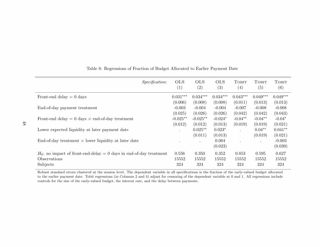
Table 8: Regressions of Fraction of Budget Allocated to Earlier Payment Date

Specification: OLS OLS OLS Tobit Tobit Tobit(1) (2) (3) (4) (5) (6)

Front-end delay = 0 days 0.031∗∗∗ 0.034∗∗∗ 0.034∗∗∗ 0.043∗∗∗ 0.049∗∗∗ 0.049∗∗∗

(0.006) (0.008) (0.008) (0.011) (0.013) (0.013)End-of-day payment treatment -0.003 -0.004 -0.004 -0.007 -0.008 -0.008

(0.025) (0.026) (0.026) (0.042) (0.042) (0.043)Front-end delay = 0 days × end-of-day treatment -0.025∗∗ -0.025∗∗ -0.024∗ -0.04∗∗ -0.04∗∗ -0.04∗

(0.012) (0.012) (0.013) (0.019) (0.019) (0.021)Lower expected liquidity at later payment date . 0.025∗∗ 0.023∗ . 0.04∗∗ 0.041∗∗

(0.011) (0.013) (0.019) (0.021)End-of-day treatment × lower liquidity at later date . . 0.004 . . -0.003

(0.023) (0.039)

H0: no impact of front-end-delay = 0 days in end-of-day treatment 0.556 0.350 0.352 0.853 0.595 0.627Observations 15552 15552 15552 15552 15552 15552Subjects 324 324 324 324 324 324

Robust standard errors clustered at the session level. The dependent variable in all specifications is the fraction of the early-valued budget allocatedto the earlier payment date. Tobit regressions (in Columns 2 and 4) adjust for censoring of the dependent variable at 0 and 1. All regressions includecontrols for the size of the early-valued budget, the interest rate, and the delay between payments.

48

Figure 1: Frequency of GARP Violations for Actual vs. Simulated Subjects

0.2

.4.6

0 1-5 6-10 11-15 16-20 More than 20

Experimental Subjects Simulated Subjects

The figure reports the total number of violations of the Generalize Axiom of Revealed Pref-erence for experimental subjects and for 1,000 thousand simulated subjects who randomizeuniformly on each budget line. Violations are calculated for the two pairs of (earlier andlater) dates that were presented at both the 400 shilling (early-valued) budget size and the600 shilling (early-valued) budget size (i.e. decision sets 1, 3, 4, and 7 from the CTB experi-ment), creating intersecting budget lines that allow for revealed preference tests.

49

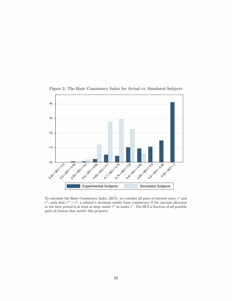
Figure 2: The Basic Consistency Index for Actual vs. Simulated Subjects

0.1

.2.3

.4

0.45

< B

CI < 0

.5

0.5

< BCI <

0.5

5

0.55

< B

CI < 0

.6

0.6

< BCI <

0.6

5

0.65

< B

CI < 0

.7

0.7

< BCI <

0.7

5

0.75

< B

CI < 0

.8

0.8

< BCI <

0.8

5

0.85

< B

CI < 0

.9

0.9

< BCI <

0.9

5

0.95

< B

CI < 1

Experimental Subjects Simulated Subjects

To calculate the Basic Consistency Index (BCI), we consider all pairs of interest rates, r′ andr′′, such that r′′ > r′; a subject’s decisions satisfy basic consistency if the amount allocatedto the later period is at least at large under r′′ as under r′. The BCI is fraction of all possiblepairs of choices that satisfy this property.

50

Figure 3: Fraction of Budget Allocated to Earlier Account, by Interest Rate

Panel A: Immediate Payouts

.3.4

.5.6

.7M

ean

frac

tion

allo

cate

d to

ear

lier

paym

ent

1 2 3 4Gross interest rate

Front end delay = 0Front end delay > 0

Panel B: End of Day Payouts

.3.4

.5.6

.7M

ean

frac

tion

allo

cate

d to

ear

lier

paym

ent

1 2 3 4Gross interest rate

Front end delay = 0Front end delay > 0

51

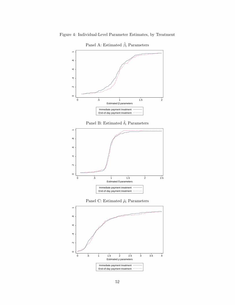
Figure 4: Individual-Level Parameter Estimates, by Treatment

Panel A: Estimated βi Parameters

0.2

.4.6

.81

0 .5 1 1.5 2

Estimated b parameters

Immediate payment treatmentEnd-of-day payment treatment

Panel B: Estimated δi Parameters

0.2

.4.6

.81

0 .5 1 1.5 2 2.5

Estimated d parameters

Immediate payment treatmentEnd-of-day payment treatment

Panel C: Estimated ρi Parameters

0.2

.4.6

.81

0 .5 1 1.5 2 2.5 3 3.5 4

Estimated r parameters

Immediate payment treatmentEnd-of-day payment treatment

52

Figure 5: Proportion of Subjects Displaying Significant Present Bias and Impatience

Panel A: Proportion of Subjects Displaying Significant Present or Future Bias0

.1.2

.3P

ropo

rtio

n of

sub

ject

s

Present-biased: b<1 Future-biased: b>1

Immediate payment treatmentEnd-of-day payment treatment

Panel B: Proportion of Subjects Displaying Significant Impatience or Patience

0.1

.2.3

.4.5

Pro

port

ion

of s

ubje

cts

Impatient: d<1 Patient: d>1

Immediate payment treatmentEnd-of-day payment treatment

53

Figure 6: The Frequency of Behavior Consistent with Arbitrage

0.1

.2.3

Pro

port

ion

of s

ubje

cts

1 2 3 4Gross interest rate

Subjects who are not liquidity-constrainedSubjects who may be liquidity-constrained

The figure plots the proportion of subjects who always allocate their entire endowment to thelater payment date at a given gross interest rate. Potentially liquidity-constrained subjectsare those who do not have at least 1,000 Kenyan shillings (USD 10.20) in a bank savingsaccount.

54

Figure 7: Per-Period Return Required to Induce Investment

0.1

.2.3

.4.5

Min

imum

req

uire

d re

turn

1 week 1 month 1 year Delay before returns are realized

Immediate payment End-of-day paymentWithout present bias Without present bias

With present bias With present bias

Bars indicate the minimum per-period return required to induce an agent to invest over threepossible time horizons, given the β and δ parameters estimated in Column 1 of Table 2. Barslabeled “without present bias” indicate the minimum required return that would induce adynamically consistent agent with the estimated level of patience (δ) to invest; this is also thelevel of return above which subjects would choose to invest if they were making commitmentsfor their future selves. Bars labeled “with present bias” indicate the marginal increase in theper-period return required to induce present-biased agents (with the observed β) to invest.

55

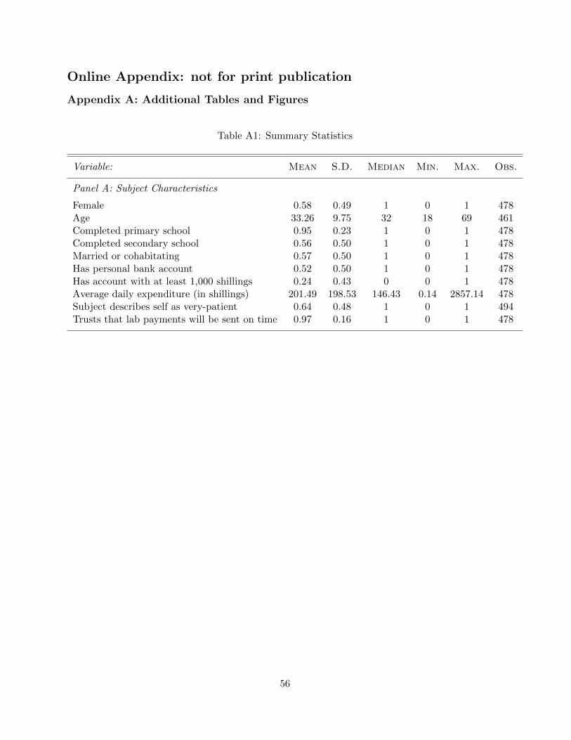
Online Appendix: not for print publication

Appendix A: Additional Tables and Figures

Table A1: Summary Statistics

Variable: Mean S.D. Median Min. Max. Obs.

Panel A: Subject Characteristics

Female 0.58 0.49 1 0 1 478Age 33.26 9.75 32 18 69 461Completed primary school 0.95 0.23 1 0 1 478Completed secondary school 0.56 0.50 1 0 1 478Married or cohabitating 0.57 0.50 1 0 1 478Has personal bank account 0.52 0.50 1 0 1 478Has account with at least 1,000 shillings 0.24 0.43 0 0 1 478Average daily expenditure (in shillings) 201.49 198.53 146.43 0.14 2857.14 478Subject describes self as very-patient 0.64 0.48 1 0 1 494Trusts that lab payments will be sent on time 0.97 0.16 1 0 1 478

56

Table A2: Summary Statistics by Experimental Treatment

Experimental Treatment:

Immediate End-of-Day

Payouts Payouts Difference

Female 0.60 0.55 0.04[0.49] [0.50] (0.05)

Age 32.79 34.35 -1.56[9.42] [10.43] (0.99)

Completed primary school 0.96 0.92 0.04∗

[0.20] [0.28] (0.02)Completed secondary school 0.55 0.59 -0.04

[0.50] [0.49] (0.05)Married or cohabitating 0.58 0.55 0.02

[0.49] [0.50] (0.05)Has personal bank account 0.53 0.51 0.01

[0.50] [0.50] (0.05)Has account with at least 1,000 shillings 0.27 0.17 0.10∗∗

[0.45] [0.38] (0.04)Average daily expenditure (in shillings) 201.54 201.37 0.16

[217.31] [146.00] (19.85)Subject describes self as very-patient 0.66 0.58 0.07

[0.47] [0.49] (0.05)Trusts that lab payments will be sent on time 0.98 0.97 0.01

[0.15] [0.18] (0.02)

Standard deviations in square brackets; standard errors in parentheses.

57

Table A3: NLS Estimates of Model Parameters — Subjects with No GARP Violations

Specification: NLS NLS NLS

(1) (2) (3)

βimmediate 0.893∗∗∗ 0.921∗∗∗ 0.928∗∗∗

(0.015) (0.014) (0.013)βeod 0.970∗∗∗ 0.981∗∗∗ 0.986∗∗∗

(0.029) (0.023) (0.025)

δimmediate 0.950∗∗∗ 0.942∗∗∗ 0.940∗∗∗

(0.011) (0.009) (0.008)δeod 0.971∗∗∗ 0.963∗∗∗ 0.956∗∗∗

(0.015) (0.012) (0.010)

ρimmediate 0.533∗∗∗ 0.860∗∗∗ 1.226∗∗∗

(0.026) (0.041) (0.111)ρeod 0.559∗∗∗ 0.887∗∗∗ 1.112∗∗∗

(0.032) (0.047) (0.090)

ωimmediate 0 ωi 522.753∗∗∗

− − (80.083)ωeod 0 ωi 404.539∗∗∗

− − (54.431)

H0: βimmediate = 1 0.000 0.000 0.000H0: βeod = 1 0.317 0.410 0.573H0: βimmediate = βeod 0.026 0.029 0.045

H0: δimmediate = 1 0.000 0.000 0.000H0: δeod = 1 0.052 0.003 0.000H0: δimmediate = δeod 0.261 0.161 0.211

H0: ρimmediate + ρeod 0.537 0.677 0.429

H0: ωimmediate + ωeod 0.229

Observations 14544 14544 14544Subjects 303 303 303

Robust standard errors clustered at the session level. ωi in-dicates self-reported average daily expenditure, which variesacross subjects.

58

Table A4: NLS Estimates of Model Parameters — Subjects with Basic Consistency Indices ≥ 0.85

Specification: NLS NLS NLS

(1) (2) (3)

βimmediate 0.918∗∗∗ 0.938∗∗∗ 0.905∗∗∗

(0.018) (0.016) (0.016)βeod 0.999∗∗∗ 1.012∗∗∗ 0.958∗∗∗

(0.031) (0.025) (0.028)

δimmediate 0.958∗∗∗ 0.951∗∗∗ 0.943∗∗∗

(0.009) (0.008) (0.009)δeod 0.977∗∗∗ 0.971∗∗∗ 0.967∗∗∗

(0.016) (0.013) (0.015)

ρimmediate 0.463∗∗∗ 0.761∗∗∗ 0.193∗∗∗

(0.018) (0.030) (0.013)ρeod 0.491∗∗∗ 0.796∗∗∗ 0.237∗∗∗

(0.019) (0.031) (0.016)

ωimmediate 0 ωi -114.747∗∗∗

− − (7.682)ωeod 0 ωi -103.761∗∗∗

− − (10.837)

H0: βimmediate = 1 0.000 0.000 0.000H0: βeod = 1 0.971 0.649 0.143H0: βimmediate = βeod 0.029 0.019 0.115

H0: δimmediate = 1 0.000 0.000 0.000H0: δeod = 1 0.163 0.030 0.040H0: δimmediate = δeod 0.299 0.200 0.184

H0: ρimmediate + ρeod 0.276 0.410 0.035

H0: ωimmediate + ωeod 0.413

Observations 15888 15888 15888Subjects 331 331 331

Robust standard errors clustered at the session level. ωi in-dicates self-reported average daily expenditure, which variesacross subjects.

59

Table A5: Convex Time Budget Decision Problems

Set Decision Front-EndDelay (t)

Early vs.Later Delay(k)

Early Max Later Max 1 + r

1 1 14 14 400 440 1.11 2 14 14 400 500 1.251 3 14 14 400 700 1.751 4 14 14 400 800 21 5 14 14 400 1200 31 6 14 14 400 1600 42 7 0 28 400 440 1.12 8 0 28 400 500 1.252 9 0 28 400 700 1.752 10 0 28 400 800 22 11 0 28 400 1200 32 12 0 28 400 1600 43 13 0 14 400 440 1.13 14 0 14 400 500 1.253 15 0 14 400 700 1.753 16 0 14 400 800 23 17 0 14 400 1200 33 18 0 14 400 1600 44 19 14 14 600 660 1.14 20 14 14 600 750 1.254 21 14 14 600 1050 1.754 22 14 14 600 1200 24 23 14 14 600 1800 34 24 14 14 600 2400 45 25 28 14 400 440 1.15 26 28 14 400 500 1.255 27 28 14 400 700 1.755 28 28 14 400 800 25 29 28 14 400 1200 35 30 28 14 400 1600 46 31 28 28 400 440 1.16 32 28 28 400 500 1.256 33 28 28 400 700 1.756 34 28 28 400 800 26 35 28 28 400 1200 36 36 28 28 400 1600 47 37 0 14 600 660 1.17 38 0 14 600 750 1.257 39 0 14 600 1050 1.757 40 0 14 600 1200 27 41 0 14 600 1800 37 42 0 14 600 2400 48 43 14 28 400 440 1.18 44 14 28 400 500 1.258 45 14 28 400 700 1.758 46 14 28 400 800 28 47 14 28 400 1200 38 48 14 28 400 1600 4

60

Table A6: Multiple Price List Decision Problems

Set Decision Front-EndDelay (t)

Early vs.Later Delay(k)

Early Max Later Max 1 + r

1 1 14 14 400 440 1.11 2 14 14 400 500 1.251 3 14 14 400 700 1.751 4 14 14 400 800 21 5 14 14 400 1200 31 6 14 14 400 1600 42 7 0 28 400 440 1.12 8 0 28 400 500 1.252 9 0 28 400 700 1.752 10 0 28 400 800 22 11 0 28 400 1200 32 12 0 28 400 1600 43 13 0 14 400 440 1.13 14 0 14 400 500 1.253 15 0 14 400 700 1.753 16 0 14 400 800 23 17 0 14 400 1200 33 18 0 14 400 1600 44 19 14 28 400 440 1.14 20 14 28 400 500 1.254 21 14 28 400 700 1.754 22 14 28 400 800 24 23 14 28 400 1200 34 24 14 28 400 1600 4

61

Figure A1: Screenshot of a CTB Decision

Figure A2: Screenshot of an MPL Decision

62

Appendix B: Experimental Instructions

This is a study of the different ways people make decisions about money. Please listen carefully to theinstructions that are being read to you. Tell us if you have any questions or if there is anything that you donot understand.

Each of you will receive two payments for participating in this study, an EARLIER payment and aLATER payment. You will receive the EARLIER payment on an EARLIER date, and you will receive theLATER payment on a LATER date. These two payments will be sent via M-Pesa by XXXX o’clock on eachdate. So, if you receive a payment today, it will be sent to you before you leave the Busara Center. On theday that you are scheduled to receive one of your payments, we will send you a text message reminder thatthe payment is coming. After you receive the text message, your payment will be sent via M-Pesa. If you donot receive one of your payments, you should immediately contact the staff at Busara by flashing +254(0)704851141

Each of you will receive 300 shillings just for participating in the study. You will receive this moneyin two equal amounts of 150 shillings. These two payments of 150 shillings will be sent to you via M-Pesaon the two different dates (the EARLIER date and the LATER date). You’ll receive your payments beforeXXXX o’clock on each date.

In addition to the 300 shillings, you will be paid money based on one of your decisions in this study. Youwill make 72 decisions in this study. The study has two parts. In the first part of the study you will make 48decisions; in the second part you will make 24 decisions. After you’ve made all 72 decisions, the computerwill choose one of the decisions to be the payment decision. We will use the payment decision to determinehow much money you are paid in this study. All 72 decisions have the same chance of being chosen as thepayment decision. So, you should make each decision as if it were the payment decision. At the end of thestudy, your computer will choose the payment decision. Because of the payment decision, you may receivemore than 150 shillings on the EARLIER date, the LATER date, or both. We will add any money from thepayment decision to your two payments of 150 shillings. So, you will receive at least 150 shillings by XXXXo’clock on each of the two dates (EARLIER and LATER). Both of these payments will be sent via M-Pesa.

In this part of the study, you will make 48 decisions about how to divide money between two times, oneis on an EARLIER date and one is on a LATER date. So, you will decide how much money you want to besent to you at the EARLIER date and how much you want at the LATER date. The easiest way to explainhow you will make decisions in this study is to show you an example.

For each decision that you will make, you will see a screen like the one that you have in front of you now.These two boxes show you when you will receive the two payments. The box on the left shows the date ofthe EARLIER payment, and the box on the right shows the date of the LATER payment. In this example,you will receive the EARLIER payment by XXXX o’clock today (before you leave the Busara Center), andyou will receive the LATER payment in two weeks later - on XXXX.

The boxes also show you the amount you will receive on each date. The box on the left shows theamount of money in the EARLIER payment, and the box on the right shows the amount of the LATERpayment. The amounts are in red. You will be paid this money in addition to the 150 shillings that you willreceive on each date (EARLIER and LATER) for participating in this study. For now, you can see that thetwo amounts are 0.

Next, notice a thick blue and green line on the center of the screen. Touch anywhere on that thick line.You should see a black pointer above the thick line and two buttons at the bottom part of the screen. Nowyou also see that the two amounts are not zero anymore.

You can change the position of the pointer moving it from right to left, or left to right by touchinganywhere on the thick line. You will see (in the two boxes) that you are moving money between theEARLIER payment and the LATER payment by touching different parts on the thick line. Thus, touchingmore towards the right side moves more money to the LATER payment from the EARLIER payment.

Please try this yourself. Touch anywhere on this thick line. As you touch more towards the left side,the amount of the EARLIER payment increases and the amount of the LATER payment decreases. Asyou touch more towards the right side, the amount of the EARLIER payment decreases and the amount of

63

the LATER payment increases. Touching more towards the right side moves more money to the LATERpayment from the EARLIER payment.

In this part of the study, you will make 48 decisions. Each decision will be different. In the boxes onthe screen, you will see the highest amounts of money that you can receive at the EARLIER and LATERdates in that decision. The highest amounts of money will not be the same in all decisions. Now practicetouching different parts of the line and changing the size of the payments. The highest amounts of moneywill not be the same in all decisions. The highest amount that you can receive on the LATER date is alwaysthe same or more than the highest amount that you can receive on the EARLIER date.

Today, you will make decisions in 8 different rounds. Each round will have 6 decisions. The dates ofthe EARLIER and the LATER payments might be different in each of the rounds. At the beginning ofeach round, we’ll announce when the EARLIER and LATER payments will take place for all the decisionsin that round. This information is also shown in the boxes on your screen.Within a round, the date of theEARLIER payment is the same for all decisions and the date of the LATER payment is the same for alldecisions.

In this part of the study, you will make 48 decisions. You will indicate your decision by touchinganywhere you want on the line. To confirm your decision, you will be touching the ”OK” button. Aftereach round, you will see a screen with the words ”Please wait for the study to continue”.

As we said earlier, the computer will choose one of your 72 decisions to be the payment decision. All 48decisions in the first part of the study have the same chance of being chosen, so you should think carefullyabout each decision.

We will start with a practice round. This practice round will be the same as the 8 later rounds. Inthis practice round, you will make 6 decisions about how you want to divide money between and EARLIERdate and a LATER date. This round is just for practice; these decisions will not be the payment decision.Remember: this round is just for practice; these decisions will not be the payment decision.

Now we will start the second part of the study. You will make 24 decisions in this part of the study. Ineach decision, you will choose between a smaller EARLIER payment and a larger LATER payment. All 24decisions in this part of the study have the same chance of being chosen as the payment decision, so youshould think carefully about each decision. The computer will choose one of the decisions to be the paymentdecision at the end of the study. So, please listen carefully to the instructions being read to you. Tell us ifyou have any questions or if there is anything that you do not understand.

The easiest way to explain how you will make decisions in this study is by showing you an example. Foreach decision that you will make, you will see a screen like the one in front of you now. These two boxesshow you when you will receive the two payments. In this example, you will receive the EARLIER paymenton XXXX, and you will receive the LATER payment two weeks LATER on XXXX. The box on the leftshows the amount of money you will receive in the EARLIER payment, and the box on the right shows theamount of money you will receive in the LATER payment. The amounts are in red colour. In this example,the EARLIER payment is XXXX, and the LATER payment is XXXX.

Each decision will be different. In each of the decisions in this study, you will see a screen like this one.You will decide if you want to receive the EARLIER payment or the LATER payment. There is no rightor wrong answer - you just choose the payment that you prefer more. To choose the EARLIER payment,touch the green ”CHOOSE THE EARLIER PAYMENT” button on the left side of the screen. To choosethe LATER payment, touch the yellow ”CHOOSE THE LATER PAYMENT” button on the right side ofthe screen. So, to make a decision, you touch the button which is below the payment that you prefer. Whenyou touch the button, its colour will turn red. To confirm your decision, you touch the ”OK” button at thebottom of you screen. You can change your decision before you touch the ”OK” button.

Today, you will make decisions in 4 different rounds. Each round will have 6 decisions. The dates ofthe EARLIER and the LATER payments will be different in every round. At the beginning of each round,well announce when the EARLIER and LATER payments will take place for all the decisions in that round.This message is also shown in the boxes on your screen.

Within a round, the date of the EARLIER payment is the same for all decisions and the date of theLATER payment is the same for all decisions. After each round, you will see a screen with the words ”Pleasewait for the study to continue.” At the end of the study, the computer will choose one of your decisions

64

to be the payment decision. All 24 decisions in this part of the study also have the same chance of beingchosen, so you should think carefully about each decision.

You will receive the payment that you chose - the EARLIER payment or the LATER payment - fromthe payment decision. If you chose the EARLIER payment and the EARLIER date is today, you will receiveyour payment before leaving Busara Center.

The computer will now choose one of your 72 decisions for payment.

65