how serious is the neglect of intrahousehold inequality?

IPolIcy, Planning,nd Research]

WORKING PAPERS

Poverty and Inequality

Office of the Vice PresidentDevelopment Economics

The World BankNovember 1989

WPS 296

How Seriousis the Neglect

of IntrahouseholdInequality?

Lawrence Haddad and Ravi Kanbur

Ignoring intrahousehold inequality can lead to considerableunderestimates of the true levels of poverty and inequality. Butthe estimated patterns of poverty and inequality across keysocioeconomic groups are not affected dramatica'lly.

The Policy. Planning, and Research Complex distributes PPR Working Papers to dtsseminate the findings of work in progress and toencourage the exchange of ideas among Bank staff and aD others interested in development issues. These papers carry the names ofthe authors, reflect only theur views, and should be used and cited accordingly. The findings, interpretauons, and conclusions a* theauthors' own. TIhey should not be autnbuted to the World Bank, its Board of Durctors, ius management, or any of its member countries.

Pub

lic D

iscl

osur

e A

utho

rized

Pub

lic D

iscl

osur

e A

utho

rized

Pub

lic D

iscl

osur

e A

utho

rized

Pub

lic D

iscl

osur

e A

utho

rized

Plc,Planning, and Research

Poverty and lneqiuality

Haddad and Kanbur developed a framework for * Patterns of inequality revealed by house-assessing the consequences of ignoring in- hold level data are somewhat different fromt-ahousehold inequality in the measurement and pattems revealed by individual level data, butanalysis of poverty and inequality. the differences seem not to be dramai . To

confirm these results, the exercise should be re-After applying this framework to data for peated with data from other countries.

the Philippines - based mainly on relativecaloric intake in households - they concluded Haddad and Kanbur's conclusions are likelythat: to be of interest to those considerinig the costly

task of surveys focused on intrahouseholde The result of neglecting intrahousehold ine- pattems in developing countries. Unless poli-

quality will probably be considerable understate- cymakers are interested primarily in morement of the levels of poverty and inequality. accurate measurement of levels of inequality andWith the Philippine data, measured levels of poverty, the exercise may not be cost-efficient.inequality and poverty were off 30 percent as aresult of ignoring intrahousehold variation.

This paper is a product of Lhe Office of the Research Administrator. Copies areavailable free from the World Bank, 1818 H Street NW, Washington DC 20433.Please contact Jane Sweeney, room S3-026, extension 31021 (39 pages with figuresand tables).

i The PPR Working Paper Series disseminates the findings of work under way in the Bank's Policy, Planning, and ResearchComplex. An objective of the series is to get these findings out quickly, even if presentations arc less than fully polished.,'he findings, interpretations, and conclusions in these papers do not necessarily repres-nt official policy of the Bank.

Produced at the PPR Dissemination Center

How Serious is the Neglect of Intrahousehold Inequality?

by Lawrence Haddadard

Ravi Kanbur

Table of Contents

1. Introduction 1

2. A Theoretical Analysis 3

3. An Empirical Analysis 14

3.1 The Data Set and the Variables 1 4

3.2 Measurement and Decomposition of Inequality 1 9

3.3 Measurement and Decomposition of Poverty 28

4. Conclusion 36

References 38

* The Authors would like to thank seminar participants at Stockholm, Leicester,Essex, Bristol, and Warwick for their helpful comments.

1

1. Introduction

In the measurenent of inequality and poverty, the

significance of intra-household inequality clearly depends on the

objective of the exercise. In the growing literature on this subject,

the reason for investigating intra-household inequality is that the

ultimate object of concern for economic policy is the well-being of

individuals. Yet most policy, and most policy analysis, has until

recently equated the well-being of individuals with the average

(adult-equivalent) well-being of the household to which they belong.

The assumption is thus that within a household resources are divided

according to need. If this were true, then policy could concentrate

on increasing the resources of poor households without getting

enmeshed in an intra-household policy that may be difficult to design

and even more difficult to execute. However, a growing body of

empirical literature has benun to question whether resources within a

household are indeed distributed according to need (see Sen, 1984;

Harris, 1986; Behrman, 1987). The natural corollary is thus that

conventional results on the extent and pattern of inequality and

poverty as revealed by household level resouroes have to be re-

examined.

There is, however, little in the way of quantification of

how much of a difference the existence of intra-household inequality

wculd make to conventional measures of inequality and poverty. Is the

understatement (if any), likely to be large? Even if the

understatement of the levels of inequality and poverty is large, are

the patterns of inequality and poverty grossly different when one

takes account of intra-household inequality? An answer to the latter

2

question is inportant since policy design (e.g. directing resouroes to

particular regions, crcp groups etc.) often relies on the pattern of

poverty and inequality (see, for example, the use by Anand (1983) of

inequality and poverty deccmposition to analyse the efficacy of

various policies in Malaysia).

The object of this paper is to present a framework in which

these questions can be addressed, and then to apply this framework, to

a data set from the Philippines on intra-household inequality in

nutritional status. Our empirical conclusions are likely to be of

interest to those who are considering undertaking the costly task of

an intra-household focused survey in developing countries. These

oonclusions can be stated very crudely but sinply as follows:

(i) The neglect of intra-household inequality is likely to lead

to a considerable understatement of the levels of inequality

and poverty.

(ii) However, while the patterns of inequality revealed by

household level data are somewhat different to those

revealed by individual level data, these differences can be

argued to be not dramatic.

The plan of the paper is as follows. The next section develops an

analytical framework for assessing the inpact of intra-household

inequality on the levels of inequality and poverty. Section 3 applies

this framework after introducing our data set. Section 4 concludes

the paper.

3

2. A Theoretical Analysis

We suppose that the object of interest is the well-being of

individuals, which is measured by some agreed standard (consumption,

nutrition etc.) and denoted y. It is assumed that all relevant

corrections and adjustments have been made and incorporated into y

(e.g. price differences, needs differences etc.) so that it really

does represent the variable on which social welfare is define;. Now

let x be the average of y within a household. Thus the

distribution of individuals by x would ignore intra-household

inequality and it is the difference between this distribution and the

distribution of y that lies at the heart of the analysis in this

paper.

Denote the conditional density of y given x as a(y| x).

This captures inequality within a household whose average standard of

living is x. If p(x) is the marginal density of x in the

population, then the density of y in the population, f (y), is

clearly

(1) f(y) = la(yi x) p(x) dx

where the integration is over the permissible range of x (perhaps

non-negative).

Notioe that by definition

(2) E(yJ x) = Iya(yj x) dy = x

4

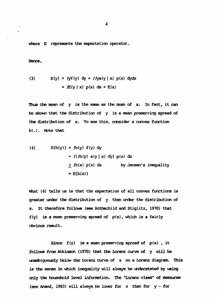
where E represents the expectation operator.

Hbnce,

(3) E(y) = Iyf(y) dy = llya(y x) p(x) dydx

= IE(yI x) p(x) dx = E(x)

Thus the mean of y is the same as the mean of x. In fact, it can

be shon that the distribution of y is a mean preserving spread of

the distribution of x. To see this, consider a convex function

h(.). Note that

(4) Efh(y)) = Ih(y) f(y) dy

= I[Jh(y) a(yl x) dyj p(x) dx

> Ih(x) p(x) dx by Jensen's inequality

= E{h(x)}

What (4) tells us is that the expectation of all convex functions is

greater under the distribution of y than under the distribution of

x. It therefore follows (see Rothschild and Stiglitz, 1970) that

f(y) is a mean preserving spread of p(x), which is a fairly

obvious result.

Since f(y) is a mean preserving spread of p(x) , it

follows from Atkinson (1970) that the Lorenz curve of y will be

unambiguously below the Lorenz curve of x on a Lorenz diagram. This

is the sense in which inequality will always be understated by using

only the household level information. The "Lorenz class" of measures

(see Anand, 1983) will always be lower for x than for y - for

5

exanple, the Gini coefficient or the Theil index will always be

understated.

To illustrate the nature of the discrepancy, consider as a

measure of inequality the coefficient of variation. Since the means

of y and x are the same, in this case we might as well use the

variance. Triting V(y) as the variance of y , V(x) as the variance

of x and V(yl x) as the variance of y conditional on x (i.e.

the variance of well-being within a household whose average well-being

is x), we know fran the analysis of variance that

(5) V(y) = N(y x) p(x) dx + V(x)

Thus the degree of discrepancy depends on what V(y | x) looks like for

different values of x . In effect, the right hand side of (5)

deconposes the inequality of y into an intra-household coxponent and

an inter-household conponent. The size of the intra-household

component - the discrepancy between V(y) and V(x) - is an empirical

matter and in the following section we provide quantification of the

discrepancy for a range of inequality measures, based on a particular

data set.

So nuch for the measured level of inequality. What about

the pattern of inequality? Suppose that our households could be split

into two mutually exclusive and exhaustive groups U and R ("urban"

and "rural"). A typical investigation of the pattern of inequality

involves two questions: (i) Which group has higher inequality? (ii)

What a fraction of inequality is accounted for by inequality within

and inequality between these two groups? These questions are asked

6

very cx mmonly in inequality analysis (e.g. Theil, 1967; Anand, 1983;

Tsakloglou, 1988) and they are inportant for policy design. Wculd the

answers differ greatly if we ignored intra-household inequality?

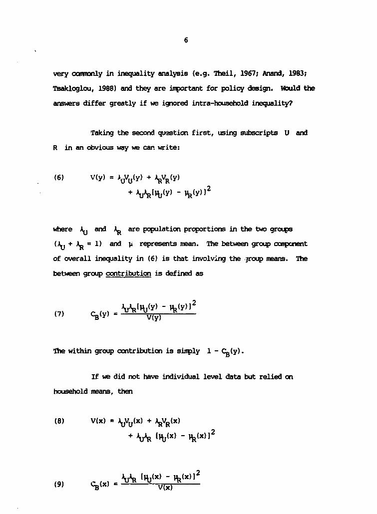
Taking the second queastion first, using subscripts U and

R in an obvious way we car write:

(6) V(y) = )AVu(Y) + ARVR(Y)

+ lAIVU(Y) - VR(y)1

where i and i are population proportions in the two groups

(AU + AR = 1) and p represents mean. The between group compcnamt

of overall inequality in (6) is that involving the .1roup means. The

between group contribution is defined as

(7) i(y) = WYAi[.VU(Y) - i.(y)J2

The within group contribution is simply 1 - C (y).

If we did not have individual level data but relied on

household means, then

(8) V(x) = AuVu(x) + ARVR(x)

+ AuAR [%(x) - PR(x)2

(9) %(x) R [j.U(x) - VR(x)12CB (x) e V(x)

7

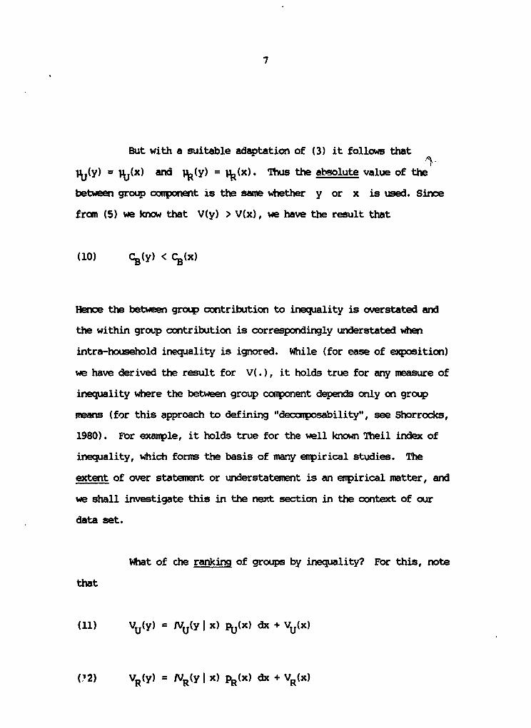
But with a suitable adaptation of (3) it follows that

a (y) = ju(x) and R (y) = R (x). Thus the absolute value of the

between group conponent is the same whether y or x is used. Since

fran (5) we know that V(y) > V(x), we have the result that

(10) C (y) < %(x)

Henoe the between group contribution to inequality is overstated and

the within group contribution is oorrespondingly understated when

intra-household inequality is ignored. While (for ease of exposition)

we have derived the result for V(.), it holds true for any measure of

inequality where the between group coomponent depends only on group

means (for this approach to defining "deccmposability", see Shorrocks,

1980). For exanple, it holds true for the well known Theil index of

inequality, which forms the basis of many empirical studies. The

extent of over statemet or understatement is an empirical matter, and

we shall investigate this in the next section in the oontext of our

data set.

What of che ranking of groups by inequality? For this, note

that

(11) VU(y) = NIU(yI x) pU(x) dx + VU(X)

(!2) VR(Y) = IVR(y I x) pR(x) dx + VR(x)

8

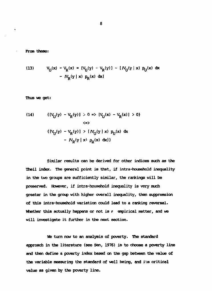
Fran these:

(13) Vu(x) VR(x) = [Vu(y) - VR(Y)J - Vu(yIx) pU(x) dx

iVR(y I x) pR(X) dx]

Thus we get:

(14) ([VU(Y) - VR(y)J I 0 => [Vu(x) - VR(x)I > 0)

{(Vu(y) VR(y)I > 1Ivu(y I X) pU (x) dx

- NR(y I x pR(x) dx])

Similar results can be derived for other indices such as the

Theil index. The general point is that, if intra-household inequality

in the two groups are sufficiently similar, the rankings will be

preserved. However, if intra-household inequality is very much

greater in the group with higher overall inequality, then suppression

of this intra-household variation could lead to a ranking reversal.

Whether this actually happens or not is e empirical matter, and we

will investigate it further in the next section.

We turn now to an analysis of poverty. The standard

approach in the literature (see Sen, 1976) is to choose a poverty line

and then define a poverty index based on the gap between the value of

the variable measuring the standard of well being, and i'cs critical

value as given by the poverty line.

9

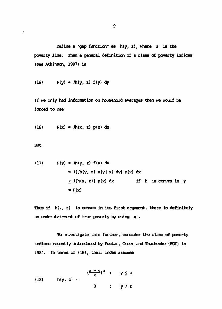
Define a gap function" as hMy, z), where z is the

poverty line. Then a general definition of a class of poverty indices

(see Atkinson, 1987) is

(15) P(y) = Jh(y, z) f(y) dy

If we only had information on household averages then we would be

forced to use

(16) P(x) = Ih(x, z) p(x) dx

But

(17) P(y) = Ih(y, z) f(y) dy

= I[Ih(y, z) a(yI x) dy] p(x) dx

> I[h(x, z)] p(x) dx if h is convex in y

= P(x)

Thus if h(., z) is convex in its first argument, there is definitely

an understatement of true poverty by using x .

To investigate this further, consider the class of poverty

indices recently introduced by Foster, Greer and Thorbecke (FG) in

1984. In terns of (15), their index assumes

O ) 0; y < zz(18) h(y, z) =

0 y>z

10

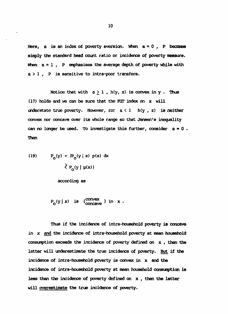
Here, a is an index of poverty aversion. When a = 0 , P beocuuss

siiply the standard head count ratio or incidence of poverty measure.

When a = 1 , P emphasises the average depth of poverty while with

a > 1 , P is sensitive to intra-poor transfers.

Notice that with a > I , h(y, z) is convex in y . Thus

(17) holds and we can be sure that the FG index on x will

understate true poverty. However, tor a < 1 h(y , z) is neither

convex nor concave over its whole range so that Jensen's inequality

can no longer be used. To investigate this further, consider a = 0

Then

(19) PO(y) = IPO(y Ix) p(X) dx

< PO(Y I P(X))

according as

P (yI x) is {conve ) in x-

Thus if the incidence of intra-household poverty is corawve

in x and the incidence of intra-household poverty at neon household

consumption exceeds the incidence of poverty defined on x , then the

latter will underestimate the true incidence of poverty. But if the

incidenoe of intra-household poverty is convex in x and the

incidence of intra-household poverty at mean household consumption is

less than the incidence of poverty defined on x , then the latter

will overestimate the true incidence of poverty.

11

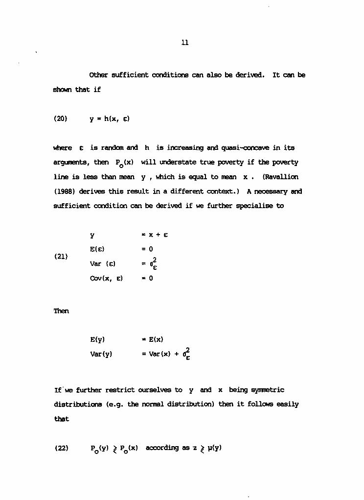
Other sufficient conditions can also be derived. It can be

shown that if

(20) y = h(x, c)

where c is randon and h is increasing and quasi-concave in its

arguments, then PO(X) will understate true poverty if the poverty

line is less than mean y , which is equal to mean x . (Ravallion

(1988) derives this result in a different context.) A ncoessary and

sufficient condition can be derived if we further specialise to

Y =X + E

E(E) =0O

(21) Var (c) =2

Cov(X, E) =0

Then

E(y) = E(x)

Var(y) = Var(x) + a2

If we further restrict ourselves to y and x being synmetric

distributions (e.g. the normal distribution) then it follows easily

that

(22) PO(Y) PO(x) according as z e3 p(y)

12

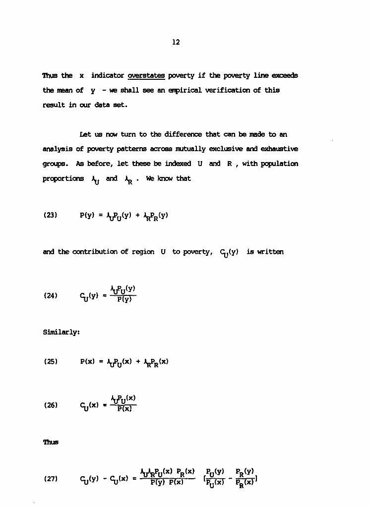
Thus the x indicator overstates poverty if the poverty line exceeds

the mean of y - we shall see an espirical verification of this

result in our data set.

Let us now turn to the difference that can be made to an

analysis of poverty patterns across mutually exclusive and exhaustive

groups. As before, let these be indexed U and R , with population

proportions Ai and i . Wb know that

(23) P(Y) = VU(Y) + ARPR(y)

and the contribution of region U to poverty, CU(y) is written

(24) C (y) = (Y)

Similarly:

(25) P(x) uPU(x) + kR(P)

(26) %(x) =vU()

CU ~~~ PRU()(x)) P(yThus

(27) %u(y) - U(x) = Ati9u(x PR(x) I PU(y)_ R)P (y) (X-) P~(x) -PR(

13

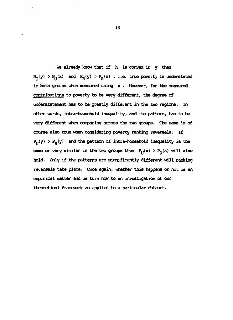
We already know that if h is convex in y then

PU(Y) > Pu(x) and PR(y) > PR(x) , i.e. true poverty is understated

in both groups when measured using x . However, for the measured

contributions to poverty to be very different, the degree of

understatement has to be greatly different in the two regicns. In

other words, intra-household inequality, and its pattern, has to be

very different when camparing across the two groups. The same is of

course also true when considering poverty ranking reversals. If

PJ(y) > PR(y) and the pattern of intra-household inequality is the

same or very similar in the two groups then Pu(x) > PR(x) will also

hold. Cnly if the patterns are significantly different will ranking

reversals take place. once again, whether this happens or not is an

empirical matter and we turn now to an investigation of our

theoretical framework as applied to a particular dataset.

14

3. An Empirical Analysis

3.1 The Data Set and the Variables

Having developed a theoretical framework and scme results on

what difference the neglect of intra-household inequality can make to

the measurement and deccnposition of inequality and poverty, it is now

time to investigate a specific dataset.

The data used in this study are described and evaluated

fully in Bcuis and Haddad (1989a). They cone from a survey of the

predominantly rural southern Philippine providence of Bukidnon. The

survey was conducted in four rounds over a sixteen month period in

1984-85, covering 448 households ccmprising 2880 individuals. The

only good for whicn we can identify individual consumption is food.

Therefore we focus on food, converting dietary intake into calories

and standardising by calorie requirements, to give calorie adequacy.

Calorie adequacy will be our measure of individual well

being. There is now a large and controversial literature on the

appropriateness of this variable for welfare and policy analysis.

However, recall that our object is to investigate the consequences of

neglecting intra-household inequality for the measurement of

inequality and poverty. Food consumption is one of the few variables

on which intra-household data can be collected and as such, is suited

to our analysis.

Calorie intakes in our data set represent 24 hour recalls by

the mDther, of food eaten by individual family menmers. This

15

information may be subject to a number of errors, both in overall

quantity recall and allocative recall. Burke and Pao (1976) review

the methodological evaluation literature for large scale surveys of

individual diets. Using the evaluation criteria of reliability (small

variable errors), validity (small biases), respondent burden, and data

oosts, they oompare 24 hour recalls with dietary history, food

weighing and inventoty-record methodologies. They conclude that "no

one methd was consistently advantageous over all others". 24 hour

recalls did well in ternm of light respondent burden and ease of

collection, but were biased to an extent primarily dependent on the

skill and probing abilities of the enumeration team. The studies

reviewed covered mainly developed countries, and we should note that

different problems may arise from their application in less developed

countries: toddler "snacking" away fran home, for instance (although

less varied LDC diets may strengthen the 24 hour recall method).

The position with respect to the 24 hour recall method is

sufmed up by Chavez and Huenemann (in Sahn et al, 1984): "Because of

the short time period, this method [24 hour recallJ is more econcmical

than the detailed method and the modified dietary history method. Cne

day may or may not represent a 'typical' intake for the individual

household. Twenty-four hour intakes of a large sample of households

may, hoyever, represent a typical daily intake for the community as a

,whole". We have minimised problems of representativeness by using

only four-round averages of calorie intake for each individual in an

attenpt to make the dietary snapshots more typical. This technique

has been used for a number of years by the USDA in its National Food

Consumption Surveys (U5CA, 1988).

16

Concerning measurement errors, two sources of evidence

attest to the accuracy of our enumerators' data collection efforts.

Firstly, calorie consumption figures calculated from two different

methodologies (24 hour recall and food expenditure data) exhibited a

high degree of correspondence at the means of the data (Bouis and

Haddad, 1989b). Furthermore, the 24 hour recall intakes corresponded

closely to a small, overlapping, subsample of food weighings conducted

simultaneously (Corpus et al, 1987).

The dencminator of the calorie adequacy ratio is calorie

requirement. We use orthodox reccuerxuded daily allowance (RDA)

calorie figures for a healthy Philippine population with requirements

diasaggregated into thirty-two age-gender-pregnancy status categories

(details in Bouis and Haddad, 1988). We recognise the limitations of

RDA's in the context in which we plan to use them. Firstly, in a

normal distribution of healthy individuals in a given age-gernder-

pregnancy-activity level group, 50% will have intakes below the RDA.

This reflects the construction of RDA's as an average requirenent

(Davidson, et al, 1979). Secondly, the requirements take no account

of an individual's unrestricted physical activity level. Even the

crude classification into limited, moderate, and extrene physical

activity is difficult to achieve in the absence of well collected

time-activity data. Thirdly, the requirenents take no account of

individual adaptation to food availability in the form of activity

patterns, longitudinal growth retardation and, to a lesser extent,

basal metabolic rate adjustment.

These problems are not trivial, but until individual

requirements for full functional capacity are available the best we

17

can do is to use the RDA's, and note that they represent "an order of

nagnitude" (Achaya, 1983).

Our object is to assess the seriousness of neglecting intra-

household inequality. In our data set, since we have individual level

data we can "pretend" that we do not have this information by taking

household averages. However, in the emvirical context we now have a

choice of whether to take the mean of individual adeuqacy ratios, or

to take the ratio of the within-household mean of individual calorie

intakes and individual requirements. There are thus three variables

of interest: individual calorie adequacy, 0 , mean individual

calorie adequacy within the household, 01, and household calorie

adequacy, 02 . Mbre precisely, let

C. = calorie intake of individual i

R. = calorie requirenent of individual i

Oi = i/Ri = calorie adequacy of individual i

n = number of individuals in household h

0 1i = n z oi = mean of individual calorie adequacy

within the household, which is

assigned to each household member.nh

= 1=1 = household calorie adequacy, which is2 nh

iRili assigried to each household me8lber.

18

Referring to our theoretical discussion, 0 corresponds to

y and 01 to x . But in the empirical rontext we typically have

to deal not with 01 but with 02 since information is collected at

the household level on calorie intake and calorie requirement

separately While 01 and 02 will differ, we shall see that the

difference, and its empirical effect, is not very great.

These three variables are calculated for all 2800

individuals in our sanple. We should note that all individuals within

a household will have identical values for 01 . The same is true

for 02 . Figure 1 shows the relative frequency plots for the three

variables. Nor surprisingly, the range for 0 is the largest of the

three. Its distribution is skewed to the right but approaches

normality. The plot for 01 is less of a normal approximation than

0 , while the plot for 02 is fairly similar to that of 01 .

The mean of 0 over the 2880 individuals in the sanple is

0.877-5, indicating that on average our sample is significantly

undernourished. The mean of 01 is by definition the same as the

mean of 0 . However, the mean of 02 is 0.88835, an excess of 1.2%,

indicating slight negative correlation between calorie intake and

calorie requirement. Or real object, however, is to examine and

compare measures of inequality and poverty defined over 0 , 01 and

02 . We start with inequality.

19

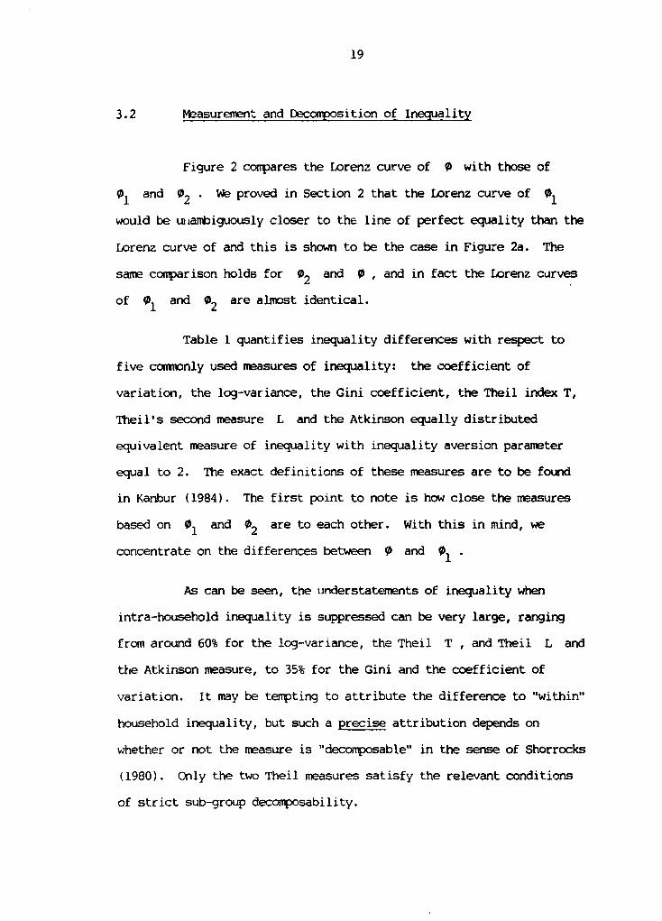
3.2 Measurement and Decomposition of Inequality

Figure 2 compares the Lorenz curve of 0 with those of

01 and 02 . We proved in Section 2 that the Lorenz curve of 01

would be uniambiguously closer to the line of perfect equality than the

Lorenz curve of and this is shown to be the case in Figure 2a. The

same comparison holds for 02 and 0 , and in fact the Lorenz curves

of 01 and 02 are almost identical.

Table 1 quantifies inequality differences with respect to

five commonly used measures of inequality: the coefficient of

variation, the log-variance, the Gini coefficient, the Theil index T,

Theil's second measure L and the Atkinson equally distributed

equivalent measure of inequality with inequality aversion parameter

equal to 2. The exact definitions of these measures are to be found

in Kanbur (1984). The first point to note is how close the measures

based on 01 and 02 are to each other. With this in mind, we

concentrate on the differences between 0 and 01

As can be seen, the understatements of inequality when

intra-household inequality is suppressed can be very large, ranging

from around 60% for the log-variance, the Theil T , and Theil L and

the Atkinson measure, to 35% for the Gini and the coefficient of

variation. It may be tempting to attribute the difference to "within"

household inequality, but such a precise attribution depends on

whether or not the measure is "decomposable" in the sense of Shorrocks

(1980). Only the two Theil measures satisfy the relevant conditions

of strict sub-group decomposability.

Figure 1. Relative Frequenc. :stributions for 0. 0 * and 02

0 - individual level

-_11 _NNNN-----

01 - individual means |

of 0 within hh

C~ ~~2 Inee _: re ;S 2 _ X Oon3<|oeg* ;2:

... ... ... .. .. .. .. .

-ratio of I ! *

household means

U ----- N _--__

21

Figure 2. Lorenz Curves for 0, 01, and 02

100 98-

70 X,./

9wqlative ., 68 -4550 ....-- --~~~~~~~~~PHI

48 ... PHI1

38-

0 18 20 38 40 58 68 70 80 98 108

ec i iis

1908

80 .. v

68-- 45~~~~~~~~~~~~~-.

tIIUlativeX i<

58 --~~~~~~~~~~~~~PHI

40. Pl 12

30 , / ,'-

28..

10.

0 8 I I 4I I I

0 10 20 30 40 58 60 78 80 90 108

geci le|

22

We turn now to the issue of the pattern of inequality as

revealed by the data. it is traditional in inequality and poverty

analysis to decompose inequality along key socio-economic dimensions.

Thus Anand (1983) provides a profile of inequality in Malayasia along

racial lines while Tsakloglou (1988) does the same exercise for Greece

along regional lines. The exact nature of the profile depends on the

policy question at hand. In the Philippine region of Bukidnon, one of

the central issues has been the impact of a move from corn to sugar

production on inequality and poverty. Bouis and Haddad (1988) provide

a detailed analysis of the nutrition and income effects of the

incroduction of sugar can cultivation in the study area. Our object

here is more limited - it is to investigate the sensitivity of the

pattern of inequality, across the sub-groups identified by Bouis and

Haddad (1989a) as being important, to the use of individual or

household level data.

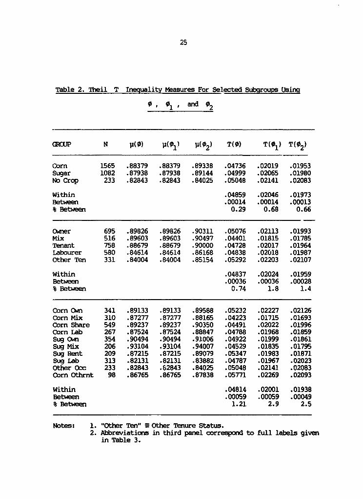
The first panel of Table 2 shows a decomposition of the

Theil T index across three mutually exclusive and exhaustive types of

households - corn producers, sugar producers and others. As can be

seen, the 2880 individuals in the sample are divided as follows: 1565

in corn producing households, 1082 in sugar producing households and

233 in other households. It is immediately seen that if we compare

inequality as measured by the Theil T index defined on 0 (individual

level data), inequality among individuals in sugar households is

greater than that among individuals in corn households, while

inequality among households that grow neither crop is greatest. A

shift in favour of sugar, perticularly if this creates landless

labourers in the process is therefore worrying from the point of view

of inequality. Would this conclusion have been greatly affected if we

Table 1. Inequality Measures for 0 , 01 , ard 02

Variable n mean oCefficient Log Variance Gini TheilT TheilL Atkinson

of Variation Coefficient (base e) (base e) Measure

(c.=2)

0 2880 .87765 .31419 .10897 .1754 .04873 .05078 .10229

01 2880 .87765 .20386 .04257 .1148 .02059 .02083 .04127

(% of 0) (65) (39) (65) (42) (41) (40)

°2 2880 .88835 .19998 .04118 .1090 .01986 .02012 .03996

(% of 0) (64) (38) (62) (41) (40) (40)

24

had had information on calorie adequacy only at the household level?

The answer is no. The inequality ranking of the three groups remains

unchanged whether 0 , 01 or 02 is used as the basis of inequality

calculations. As was pointed out in Section 2, for ranking reversals

to take place it has to be the case that patterns of intra-household

inequality are vastly different from group to group - this is clearly

not the case for our data set.

An alternative dimension to be considered is tenure status.

As Bouis and Haddad (1989a) document, households which managed to

overcome the barriers to entry of sugar cane cultivation (i.e. those

who secured a mill contract, with sufficient credit, and were close

enough to the mill so as not to make transport costs prohibitive)

realised substantial increases in agricultural profits. However, for

every household able to capitalise on the mill start-up there was a

household that experienced a degradation in tenure status. Because of

the low profits earned on corn cultivation, landowners unable to

overcome the barriers to sugar cane cultivation were tempted into

short-run capital gains through selling their land and then selling

their labour. Some pre-sugar share-tenants were sinply evicted by

landowners eager to reap the sugar cane profits, and were replaced by

migrant cane labourers.

The second panel in Table 2 provides intra-group

inequalities based on 0 , 0 1 and 02 for five tenure status groups.

once again, we see that the rankings remain unaffected. The lowest

inequality is among households that have a mixed owner/renter status,

with pure tenancy status coming next, followed by labourers, owners,

25

Table 2. Theil T Inequality Measures For Selected Subgroups Using

0 01 , and 02

GRCUP N p(0) p(01) p(02) T(O) T(01 ) T(02 )

Corn 1565 .88379 .88379 .89338 .04736 .02019 .01953Sugar 1082 .87938 .87938 .89144 .04999 .02065 .01980No Crop 233 .82843 .82843 .84025 .05048 .02141 .02083

Within .04859 .02046 .01973Between .00014 .00014 .00013% Between 0.29 0.68 0.66

owner 695 .89826 .89826 .90311 .05076 .02113 .01993Mix 516 .89603 .89603 .90497 .04401 .01815 .01785Tenant 758 .88679 .88679 .90000 .04728 .02017 .01964Labourer 580 .84614 .84614 .86168 .04838 .02018 .01987Other Ten 331 .84004 .84004 .85154 .05292 .02203 .02107


Corn Own 341 .89133 .89133 .89588 .05232 .02227 .02126Corn Mix 310 .87277 .87277 .88165 .04223 .01715 .01693Corm Share 549 .89237 .89237 .90350 .04491 .02022 .01996Corn Lab 267 .87524 .87524 .88847 .04788 .01968 .01859Sug Own 354 .90494 .90494 .91006 .04922 .01999 .01861Sug Mix 206 .93104 .93104 .94007 .04529 .01835 .01795Sug Rent 209 .87215 .87215 .89079 .05347 .01983 .01871Sug Lab 313 .82131 .82131 .83882 .04787 .01967 .02023Other Ooc 233 .82843 .62843 .84025 .05048 .02141 .02083Corm Othrmt 98 .86765 .86765 .87838 .05771 .02269 .02093


Notes: 1. "Other Ten" - Other Tenure Status.2. Abbreviations in third panel correspond to full labels given

in Table 3.

26

and other teure status l duseholds. This inquality rancing w

maintained wtether irixvidual level or thouehold level informtion ws

uwed. Clearly, then, the ectra infornntion of intra4muehold

irequaity does not affect the conclusion an patterm of irmquaity at

this level of disaggregation, ed therefore any calusions that mrght

follow an the oox-euke for overall irality of the introduction

of sugar cultivation.

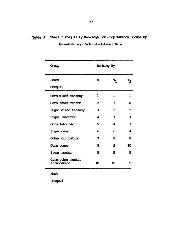
11h final level of dis tion we tried s that given in

the third panel of Table 2, where ten niully ecluive ad

exdaustive groups of houeholds are identified aooording to crop and

tenure status. We would especi, of course, that as the digrergation

bexmnnes finer and firer and groups b1xxzne more hmrigenous , eventually

rarng chiaqs would begin to aear. Table 3 show the rarks in

question. Using 9 the oorn/imed tenarncy group is the least ureqLul

while the corrVother rental arrangeint group is most urqual. Ahe

saw is true if we use 0, . With 02 the oor/mixed grOxp is still

least uequal but the corr/cwner grouxp is now rlt unequal. Acoording

to the 1 and 0 ranirgs the corr/owner groups is 8th nvmt unqual

and 9th most ursxqul r emctively. in order to get a quLwtitative

feel for the extent of rank reversal we calculated SpeaEnls rink

correlation coefficients. The rank correlation coefficient bebieen

01 and 02 is 0.85, indicating very close association between the

tbo ranks. That be n 0 and 01 is 0.72. IThe lowst value for

the coefficient is betwe 0n *and *2 is 0.66. urn we cm candCude

that the extent of rank dhwiges when we msiadh fro indivi&.l bo

household level data is significant but not dreamtic.

27

Table 3: Theil T Inequality Rankings For Crop-Tenancyv Groups By

Household and Individual-Level Data

Group Ranking By

Least 0 01 02

Unequal

Corn mixed tenancy 1 1 1

Corn share tenant 2 7 6

Sugar mixed tenancy 3 2 2

Sugar labourer 4 3 7

Corn labourer 5 4 3

Sugar owner 6 6 4

other occupation 7 8 8

Corn owner 8 9 10

Sugar renter 9 5 5

Corn other rentalarrangement 10 10 9

nbst

Unequal

28

Finally, fron Table 2 we note the enpirical confirmation of

our theoretical result that the between group cxnponent of inequality

will be unchanged whether 0 or 01 is used, sinoe this depends

only on group means and the conditional mean of 0 is the same as the

conditional mean of 01 for any conditioning variable. Since the

within group cxponent of inequality is irevitably greater with 0

than with 01 , it follows that the contribution of this component

to total inequality when 0 is used is greater than when 01 is

used. Correspondingly, with 0 the contribution of the between group

component is lower than with 01 . Tn our dataset, these conslusions

are unchanged when 01 is replaced by 02 .

3.3 Measurement and Deccnvosition of Poverty

In Section 2 we derived a number of theoretical results on

the likely inpact of intra-household inequality on measured poverty.

The object of this subsection is to consider an eapirical analysis

based on our data set. Any neasurenent of poverty requires us to

specify a poverty line. In the context of the variable of interest in

this study - the calorie adequacy ratio - an appropriate poverty line

is siuply 1. All those with calorie adequacy ratio less than 1 can

reasonably be argued to be undernourished or "poor" in the terminology

of income puverty. We will concentrate attention on the class of

poverty indices put forward by Ebster, Greer and Thorbecke (1984).

Adapting the notation of (15) and (18), these can be written as

I1

29

where 0 is calorie adequacy, f(.) its frequency density, and a is

the poverty aversion parameter. We focus on Q = 0, 1, 2 in our

discussion.

Table 4 presents values of PO , P1 . and P2 based on

0 , 01 , and 02 . we have already provAx that for a > 1 Pa for

0 will exceed PQ for 01 . This is seen in the table. Ignoring

intra-household inequality leads to an understatement of P1 of 18.4*

if 01 is used and 23.0% if 02 is used. Similarly, if P2 is the

accepted index of poverty then there is an understatenent of 39.4%

with 01 and 44.4% with 02 . Clearly, then, there is a dramatic

understatement of poverty if intra-household inequality is ignored,

for a> 1 .

However, notice with with a = 0 the situation is

the other way round, there is now a significant overstatement of

poverty if intra-houshehold inequality is ignored. Using 0 there

are 70.2% of individuals below the calorie adequacy ratio of 1, while

using 01 76.9% of individuals fall below this critical value - an

overstatement of 9.4%. The explanation for this reversal is to be

found in equation (22) of Section 2. Under certain conditions we

showed that the incidenoe of poverty (or under-nutrition) will be

overstated by household level data if the poverty line exceeds the

population mean. This is exactly what happens in our data - the

mean of 0 (and 01) is 0.88 while the chosen poverty line is 1.00.

30

Table 4. Poverty Measures For 0 , 01 and 02

Variable n Mean PO Pi P2

0 2880 .87765 .70243 .18640 .06759

01 2880 .87765 .76875 .15201 .04093

02 2880 .88835 .75764 .14355 .03756

Note: P , P1 ,and P2 are the P. class of indices where

= 0, 1, 2

31

Table 5. P Poverty Measures For Selected Subgroups Using 0,

01 , and 02

RaJP N P0 (0) P(o) P2(0) Poo0 (0 1) P22(01) Po(02) P1(02) P2(02)

ALL 2880 .70243 .18640 .06759 .76875 .15201 .04093 .75764 .14355 .03756

Corn 1565 .69521 .18144 .06483 .75463 .14661 .03925 .73738 .13897 .03632Sugar 1082 .70055 .18592 .06811 .77634 .15042 .04029 .77172 .14125 .03647No Crop 233 .75966 .22203 .08369 .82833 .19571 .05516 .82833 .18494 .05097

cwner 695 .68345 .17584 .06342 .74964 .14021 .03716 .74964 .13459 .03495Mix 516 .67636 .17171 .05930 .70543 .13731 .03354 .72093 .13092 .03137Tienmt 758 .688(3 .17792 .06445 .76253 .14202 .03822 .74802 .13265 .03441Labourer 580 .743:0 .20589 .07605 .83276 .17269 .04884 .78276 .16133 .04424Other Ten 331 .74320 .21676 .08159 .80967 .18633 .05270 .80967 .17582 .04822

Corn Own 341 .68622 .18359 .06663 .73607 .14803 .03970 .73607 .14226 .03797Corn Mix 310 .71613 .18241 .06382 .70968 .15507 .03895 .70968 .14857 .03646Corn Share 549 .68852 .17219 .06080 .76138 .13601 .03740 .74499 .12825 .03452Corn Lab 267 .69288 .18820 .06766 .81273 .15036 .04007 .74532 .14009 .03578Sug Own 354 .68079 .16837 .06034 .76271 .13269 .03472 .76271 .12720 .03204Sug Mix 206 .61650 .15562 .05250 .69903 .11059 .02541 .73786 .10435 .02370Sug Rent 209 .68900 .19298 .07404 .76555 .15781 .04037 .75598 .14421 .03412Sug Lab 313 .78594 .22099 .08320 .84984 .19174 .05632 .81470 .17946 .05146Other Ooc 233 .75966 .22203 .08369 .82833 .19571 .05516 .82833 .18494 .05097Corn Orthnt 98 .70408 .20423 .07661 .76531 .16404 .04685 .76531 .15414 .04168

Male 1484 .72372 .19017 .06863 .77089 .15058 .04016 .76146 .14262 .03691Female 1396 .67980 .18240 .06648 .76648 .15353 .04175 .75358 .14453 .03826

Adult* 1191 .48615 .10074 .03259 .75231 .14757 .03957 .74139 .13920 .03633Non Adult 1689 .85494 .24681 .09226 .78034 .15515 .04189 .76909 .14661 .03843

* Non-Adults are defined as individuals less than or equal to nineteen years of agein accordance with definitions employed by the National Nutrition Council of thePhilippines for calorie requirements. (NNC, 1976).

32

Table 6. P1 Poverty Rankings For Crqp-Tenancy Groups by

Household and Individual-Level Data

Group Ranking By

Least Poverty 0 01 02

Sugar mixed tenancy 1 1 1

Sugar owner 2 2 2

Corn share tenant 3 3 3

Corn mixed tenancy 4 6 7

Corn owner 5 4 5

Corn labourer 6 5 4

Sugar renter 7 7 6

Corn other rentalarrangement 8 8 8

Sugar labourer 9 9 9

Other occupation 10 10 10

Most poverty

33

Let us turn now to the pattern of poverty across socio-

ecooncmic groups. Table 5 presents group values of P. indices.

The first three panels of Table 5 use the same mutually exclusive and

exhaustive groups as in Table 2. The policy relevance of these

household level grouping has already been discussed in Section 3.2.

The theoretical significance of PQ rankings of sectors

and groups has been discussed by Kanbur (1987) in the context of

targeting and poverty alleviation. We note here that there are no

ranking changes in the first or the second panel. As argued earlier,

we would expect some rank changes to occur as the classification gets

finer. However, even with 10 groups the changes are very small.

Table 6 summarises the rankings for the P1 measure. As can be seen,

the three poorest and three least poor groups in the ranking are

unchanged as between 0 , 01 and 02 . The rank correlation

coefficient between 0 and 01 is (0.96) and that between 0 and

01 is (0.96) and that between 0 and 02 is (0.9). Clearly, then

the neglect of intra-household inequality is not leading to dramatic

changes in poverty ranking.

The groupings used so far, and those discussed in the

theoretical section, are those defined at the Ihusehold level. Ebr

som policy purposes, hotever, individual level groupings are required.

The last two panels in Table 5 consider two such groupings which are

of obvious interest - male/female and adult/non-adult. The adult/non-

adult division reveals no P. ranking differences as between 0 ,

01 and 02 . However, we find that iale-female P1 and P2 rankings

are reversed when oomparing 0 with 01 and 0 with 02 . This

34

could be potentially serious if targeting policy towards males and

females (for exanple in supplemental feeding programmes) is to be

based on the degree of observed under-nutrition in these groups.

However, this is the only case, in all of the deconpositions in Table

5, where rank reversal is potentially serious.

Finally, we consider group contributions to poverty based on

0 , 01 and 02 . Table 7 presents this analysis. The first four

panels in Table 7 show the similar contributions each group makes to

overall poverty whether we use 0 , 01 , or 02 . As we argued

earlier, intra-household inequality would have to be very different

when conparing across groups for the contributions to poverty to

differ by much.

Although the only individual-level grouping that experienoes

a ranking reversal in Table 5 is the male/fenale classification, the

difference between adult/non-adult poverty levels widens substantially

as we move from poverty measures based on 01 and 02 , to those

based on 0 . This is emphasised in the bottcm panel of Table 7,

which shows the non-adult contribution to poverty measures based on 0

be in the 70-80% range, but falling to 60% when 01 and 02 are

used.

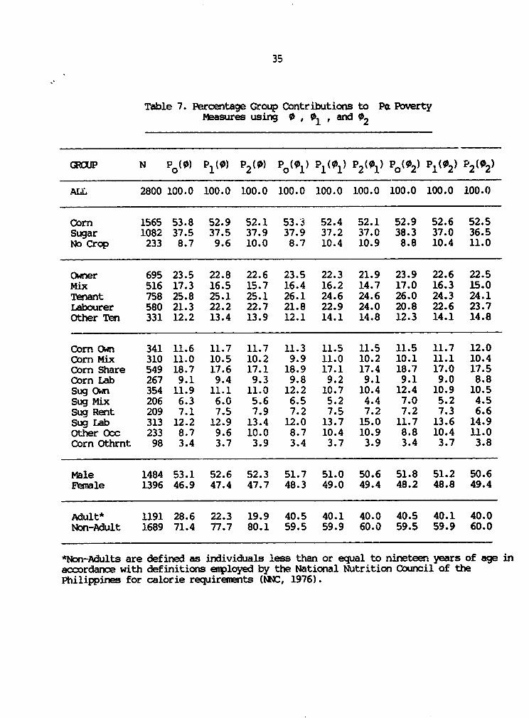
35

Table 7. Percentage Group Contributions to Pe PovertyMeasures using 0 , 01 , and 02

CQOlJP N Po(0) P1(0) P2(0) Po(01) P (01) P2(01) Po(02) 1 2 2 2

ALL 2800 100.0 100.0 100.0 100.0 100.0 100.0 100.0 100.0 100.0

Corn 1565 53.8 52.9 52.1 53.3 52.4 52.1 52.9 52.6 52.5Sugar 1082 37.5 37.5 37.9 37.9 37.2 37.0 38.3 37.0 36.5No Crop 233 8.7 9.6 10.0 8.7 10.4 10.9 8.8 10.4 11.0

Owner 695 23.5 22.8 22.6 23.5 22.3 21.9 23.9 22.6 22.5mix 516 17.3 16.5 15.7 16.4 16.2 14.7 17.0 16.3 15.0Tenant 758 25.8 25.1 25.1 26.1 24.6 24.6 26.0 24.3 24.1Labourer 580 21.3 22.2 22.7 21.8 22.9 24.0 20.8 22.6 23.7Other Ten 331 12.2 13.4 13.9 12.1 14.1 14.8 12.3 14.1 14.8

Com Own 341 11.6 11.7 11.7 11.3 11.5 11.5 11.5 11.7 12.0Corn Mix 310 11.0 10.5 10.2 9.9 11.0 10.2 10.1 11.1 10.4Corn Share 549 18.7 17.6 17.1 18.9 17.1 17.4 18.7 17.0 17.5Corn Lab 267 9.1 9.4 9.3 9.8 9.2 9.1 9.1 9.0 8.8Sug Own 354 11.9 11.1 11.3 12.2 10.7 10.4 12.4 10.9 10.5Sug Mix 206 6.3 6.0 5.6 6.5 5.2 4.4 7.0 5.2 4.5Sug Rent 209 7.1 7.5 7.9 7.2 7.5 7.2 7.2 7.3 6.6Sug Lab 313 12.2 12.9 13.4 12.0 13.7 15.0 11.7 13.6 14.9Other Oxc 233 8.7 9.6 10.0 8.7 10.4 10.9 8.8 10.4 11.0Corn Othrnt 98 3.4 3.7 3.9 3.4 3.7 3.9 3.4 3.7 3.8

Male 1484 53.1 52.6 52.3 51.7 51.0 50.6 51.8 51.2 50.6Female 1396 46.9 47.4 47.7 48.3 49.0 49.4 48.2 48.8 49.4

Adult* 1191 28.6 22.3 19.9 40.5 40.1 40.0 40.5 40.1 40.0Non-Adult 1689 71.4 77.7 80.1 59.5 59.9 60.0 59.5 59.9 60.0

*Non-Adults are defined as individuals less than or equal to nineteen years of age inaccordance with definitions employed by the National Nutrition Council of thePhilippines for calorie requirements (NNC, 1976).

36

4. Conclusion

The object of this paper has been, firstly, to develop a

framework in which the consequences of ignoring intra-household

inequality for the measurement and decomposition of inequality and

poverty can be assessed arnd, secondly, to applv this framework to a

particular dataset. Our theoretical analysis suggested that

potentially serious errors could be made so far as the levels of

inequality and poverty are concerned. Emipirically, we showed that

this is indeed the case - the errors are of the order of 30% or more.

In the case of poverty measurement we showed theoretically and

empirically that for certain measures of poverty the errors could be

of either sign - a careful analysis is therefore required before any

claims are made as to whether poverty is understated or overstated.

So far as the patterns of inequality and poverty are

concerned, our theoretical analysis was more equivocal - significant

differences in the cross group patterns of intra-household inequality

are required to reverse the true rankings of policy-relevant socio-

economic groups by inequality and poverty, when intra-household

inequality is ignored. Our cmpirical analysis lends support to this

equivocation - the changes in patterns of inequality when intra-

household inequality is ignored are by no means dramatic; sometimes,

they hardly change at all.

There is clearly a need to further confirm our results for

other data sets in other countries. We hope to have provided both a

framework in which such analysis can proceed and a preliminary

indication that the results are inportant to policy makers who are

37

considering whether or not to launch a costly intra-household oriented

survey. The conclusions based on our data set are that the collection

of such data is inportant if the object is to get an estimate of the

levels of inequality and poverty; but if the object is to discover the

patterns of inequality and poverty across key socio-econcxnic groups,

the policy maker would do well to assess carefully the costs and

benefiUs of such an exercise.

38

RENCES

Achaya, K. T. (1983), 'RDAs: Their Limitations and Application',Economic and Political Weekly, XVIII (15), April, p. 587.

Anand, S. (1983), Inequality and Poverty in Malaysia: Measurement andDeoamposition, Oxford University Press.

Atkinson, A. B. (1970), 'On the Measurement of Inequality', Journal ofEconcmic Theory.

Atkinson, A. B. (1987), 'On the Measurement of Poverty', Eoonometrica.

Behrman, J. (1987), 'Intrahousehold Allocation of Nutrients and GenderEffects', University of Pennsylvania, Philadelphia, mimeo.

Bouis, H.E. and L. J. Haddad (1989a) A Case Study of thenomnercialisation of Aqricultuie in the Southern Philippines:

The Income, Consunption and Nutrition Effects of a SwitchFrcm Corn to Sugar Production in Bukianon, ForthomingResearch Report, IFPRI, Washington D.C.

Bouis, H. E. and L. J. Haddad (1989b), 'Estimating the Relationshipbetween Calories and Incote: Does Choice of Survey VariableMatter?', IFPRI, mimreo, Washington D. C.

Burke, M. and E. Pao (1976), 'Methodology for Large-Scale Surveys ofHousehold and Individual Diets', USDA, Home EconomicsResearch Report No. 40, Washington D. C.

Chavez, M. and R. Huenemann (1984), 'Measuring Impact by AssessingDietary Intake and Food Consumption', in Methods for theEvaluation of the Impact of Food and Nutrition Programnes,edited by D. Sahn, R. Lockwood and N. Scrimshaw, UNU.

Corpus, V.A., A. Ledesma, A. Limbo and H. Bouis (1987), 'TheCobmercialisation of Agriculture in the Southern Philippines.Phase I Report', mimeo, IFPRI, Washington D.C.

Davidson, S., R. Passmore, J. F. Brock and A. S. Truswell (1979),Human Nutrition and Dietics (7th edition), ChurchillLivingstone.

Foster, J., J. Greer and E. Thorbecke (1984), 'On a Class ofDeconpeable Poverty Measures', Econametrica.

Harris, B. (1986), 'The Intra Family Distribution of Hunger in SouthAsia', fortkxoming in J. Dreze and A. K. Sen (ed.) Hungerand Public .'olicy, Oxford University Press.

Kanbur, R. (1984), 'The Measurment and Deccnposition of Inequality andPoverty' in Mathemdtical Methods in Economics, edited by F.van der Ploeg, Academic Press.

Kanbur, R. (1987), "Measurement and Alleviaticn of Poverty", I.M.F.Staff Papers

39

NNC (1976), 'Philippine Recammerded Dietary Allowanees', Part 1,National Nutrition Council of the Philippines.

Ravallion, M. (1988), 'Expected Poverty Under Risk Induoed WelfareVariability', Economic Journal.

Rothschild, M. and J. E. Stiglitz (1970), 'Increasing Risk I: ADefinition, Journal of Economic Theory.

LEM (1988), Nationwide Food Consuuption Survev Continuinq Survey ofFood Intakes by Individuals, Human Nutrition InformationService, NFCS, CSFII, No. 86-3.

Sen, A. K. (1976), 'Poverty: An Ordinal Approach to Measurement',Econometrica.

Sen, A. K. (1984), 'Family and Food: Sex Bias in Poverty', in A. K.Sen, Resources, Values and Deve1oprsent, Blackwell.

Shorrocks, A. F. (1980), 'The Class of Additively DeccuposableInequality Measures', Econometrica

Theil, H. (1967), Economics and Information Theory, North Holland.

Tsakloglou, P. (1988), 'Aspects of Inequality and Poverty in Greece',Unpublished Ph.D. Dissertation, University of Warwick.

PPR Working Paper Series

Contactid% AtAhor Da1a for paper

WPS279 What Determines the Rate of Paul M. Romer September 1989 R. LuzGrowth and Technological Change 61760

WPS280 Adjustment Policies in East Asia Bela Balassa September 1989 N. Campbell33769

WPS281 Tariff Policy and Taxation in Bela Balassa September 1989 N. CampbellDeveloping Countries 33769

WPS282 EMENA Manufactured Exports Bela Balassa September 1989 N. Campbelland EEC Trade Policy 33769

WPS283 Experiences of Financial Distress Tipsuda Sundaravejin Thailand Prasarn Trairatvorakul

WPS284 The Role of Groups and Credit Gershon Feder October 1989 C. SpoonerCooperatives in Rural Lending Monika Huppi 30469

WPS285 A Multimarket Model for Jeffrey S. Hammer October 1989 P. PlanerTurkish Agriculture Alexandra G. Tan 30476

WPS286 Poverty and Undernutrition in Martin Ravallion September 1989 C. SpoonerIndonesia During the 1980s Monika Huppi 30464

WPS287 The Consistency of Government Thanos Catsambas October 1989 M. RuminskiDeficits with Macroeconomic Miria Pigato 34349Adjustment: An Application toKenya and Ghana

WPS288 School Effects and Costs for Emmanuel Jimenez October 1989 C. CristobalPrivate and Public Schools in Marlaine E. Lockheed 33640the Dominican Republic Eduardo Luna

Vicente Paqueo

WPS289 Inflation and Seigniorage in Miguel A. Kiguel October 1989 R. LuzArgentina Pablo Andr6s Neumeyer 61588

WPS290 Risk-Adjusted Rates of Return Avinash Dixit November 1989 C. Spoonerfor Project Appraisal Amy Wiilliamson 30464

WPS291 How Can Indonesia Maintain Sadiq Ahmed October 1989 M. ColinetCreditworthiness and Noninflationary Ajay Chhibber 33490Growth?

WPS292 Is the New Political Economy Ronald Findlay November 1989 R. LuzRelevant to Developing Countries? 61588

WPS293 Central Bank Losses: Origins, Mario 0. Teijeiro October 1989 R.LuzConceptual Issues, and Measurement 61588Problems

PPR Working Paper Series

Contact

id%a Author .X1fl. for paper

WPS294 Irreversibility, Uncertainty, and Robert S. Pindyck October 1989 N. CarolanInvestment 61737

WPS295 Developing Country Experience Vinod Thomas October 1989 S. Fallonin Trade Reform 61680

WPS296 How Serious is the Neglect of Lawrence Haddad November 1983 J. SweeneyIntrahousehold Inequality? Ravi Kanbur 31021

WPS297 Effects of the Multi-Fibre Refik Erzan November 1989 L. TanArrangement on Developing Junichi Goto 33702Countries' Trade: An Empirical Paula HolmesInvestigation

WPS298 Evaluation and Validation of a Multi- Ahmad JamshidiRegion Econometric Model: A CaseStudy of MULTIMOD: A Forward-LookingMacroeconometric Model

WPS299 The External Effects of Public Carlos Alf redo Rodriguez November 1989 R. LuzSector Deficits 61588

WPS300 How the 1981-83 Chilean Banking Mauricio LarrainCrisis was Handled

WPS301 Myths of the West: Lessons from Collin Mayer November 1989 WDR OfficeDeveloped Countries for Development 31393Finance

WPS302 Improving Support Services for Sherry KeithRural Schools: A ManagementPerspective

WPS303 Is Undernutrition Responsive to Martin Ravallion November 1989 C. SpoonerChanges in Incomes? 30464

WPS304 The New Political Economy: Merilee S. GrindlePositive Economics and NegativePolitics

WPS305 Between Public and Private: A Lawrence F. SalmenReview of Non-Governmental A. Paige EavesOrganization Involvement in WorldBank Projects

WPS306 A Method for Macroeconomic Ali KhadrConsistency in Current and Klaus Schmidt-HebbelConstant Prices

how serious is the neglect of intrahousehold inequality?

Documents