NBER WORKING PAPER SERIES

HOW JOHNSON FOUGHT THE WAR ON POVERTY:THE ECONOMICS AND POLITICS OF FUNDING AT THE OFFICE OF ECONOMIC OPPORTUNITY

Martha J. BaileyNicolas J. Duquette

Working Paper 19860http://www.nber.org/papers/w19860

NATIONAL BUREAU OF ECONOMIC RESEARCH1050 Massachusetts Avenue

Cambridge, MA 02138January 2014

This project was supported by the National Institutes of Health (Grant HD058065-01A1 and R03-HD066145), the National Bureau of Economic Research’s Dissertation Grant for the Study of the NonprofitSector (2011-2012), the Economic History Association’s Exploratory Data Collection Grant (2011),and the Rackham Centennial Graduate Fellowship (2012). We gratefully acknowledge the use of theservices and facilities of the Population Studies Center at the University of Michigan (funded by NICHDCenter Grant R24 HD041028). We are indebted to Price Fishback for editorial guidance and extensivecomments. We are also grateful to Bill Collins and Bob Margo for providing their measures of riotintensity; to Price Fishback, Paul Rhode, and Michael Haines for sharing their information on farmoperators in the 1930s; and to Paul Rhode for sharing information on the U.S. census plantation counties.We also thank Lee Alston, Sheldon Danziger, Daniel Eisenberg, Joe Ferrie, Price Fishback, DavidLam, Robert Margo, Edie Ostapik, Marit Rehavi, Paul Rhode, Mel Stephens, Jeff Smith, John Wallis,Gavin Wright and participants at the 2012 Cliometrics Society Meeting for helpful comments andsuggestions. The views expressed herein are those of the authors and do not necessarily reflect theviews of the National Bureau of Economic Research.

NBER working papers are circulated for discussion and comment purposes. They have not been peer-reviewed or been subject to the review by the NBER Board of Directors that accompanies officialNBER publications.

© 2014 by Martha J. Bailey and Nicolas J. Duquette. All rights reserved. Short sections of text, notto exceed two paragraphs, may be quoted without explicit permission provided that full credit, including© notice, is given to the source.

How Johnson Fought the War on Poverty: The Economics and Politics of Funding at the Officeof Economic OpportunityMartha J. Bailey and Nicolas J. DuquetteNBER Working Paper No. 19860January 2014, Revised September 2014 JEL No. H50,J08,N12

ABSTRACT

This paper presents a quantitative analysis of the geographic distribution of spending through the 1964Economic Opportunity Act (EOA). Using newly assembled state- and county-level data, the resultsshow that the Johnson administration directed funding in ways consistent with the War on Poverty’srhetoric of fighting poverty and racial discrimination: poorer areas and those with a greater share ofnonwhite residents received systematically more funding. In contrast to New Deal spending, politicalvariables explain very little of the variation in EOA funding. The smaller role of politics may helpexplain the strong backlash against the War on Poverty’s programs.

Martha J. BaileyUniversity of MichiganDepartment of Economics611 Tappan Street207 Lorch HallAnn Arbor, MI 48109-1220and NBERbaileymj@umich.edu

Nicolas J. DuquetteUniversity of Michigannduquett@umich.edu

Appendices available at http://www.nber.org/data-appendix/w19860

1

In his first State of the Union address in January 1964, President Lyndon B. Johnson asked Congress

to declare an “unconditional war on poverty” and to aim “not only to relieve the symptom of poverty, but

to cure it and, above all, to prevent it” (1965). Over the next five years, Congress passed legislation that

transformed American schools, launched Medicare and Medicaid, and expanded housing subsidies, urban

development programs, employment and training programs, food stamps, and Social Security and welfare

benefits. These programs more than tripled real federal expenditures on health, education, and welfare,

which grew to over 15 percent of the federal budget by 1970 (Ginzberg and Solow 1974).

Using the volumes of oral histories, taped conversations, and archival documents, historians have

pieced together competing (but not mutually exclusive) narratives of this decade’s political economy

(Gettleman and Mermelstein 1966; Levitan 1969; Ginzberg and Solow 1974; Davies 1996; Gillette 1996;

O’Connor 2001; Germany 2007; Orleck and Hazirjian 2011; Caro 1982, 2002, 2012). Economic

historians attribute the policy shift in the 1960s to a long-term decline in Southern planters’ demand for

cheap agricultural workers and accompanying decline in plantation paternalism (Alston and Ferrie 1993,

1999). Relative to the large literature that examines the political economy of the New Deal, little

quantitative research has considered the political economy of the War on Poverty: how and why it

evolved from the small-scale, academic brainchild of the Council of Economic Advisors to a

controversial and enduring legacy of the Johnson presidency.1

This paper contributes a novel quantitative description to the vast narrative, documentary, and oral

history of the 1960s political economy. We analyze how the War on Poverty was fought through the lens

of the legislation that came to define it: the 1964 Economic Opportunity Act (EOA).2 This centerpiece

legislation created the Office of Economic Opportunity (OEO) to coordinate federal antipoverty

initiatives and empower the poor to transform their own communities. The EOA also contained two

1 Many reasons recommend a separate treatment of the two periods. The New Deal was developed in response to high unemployment and the economic crisis of the Great Depression; Johnson launched the War on Poverty during a period of widely shared economic prosperity. The New Deal significantly expanded programs cooperatively administered between the federal and state governments (Fishback and Wallis 2012, p. 291), whereas the federal government retained the purse strings and discretionary power for many of the War on Poverty programs. Finally, the New Deal built on and expanded many existing national programs (public infrastructure, benefits to veterans, agricultural assistance, and emergency loans for farmers) and significantly expanded unemployment relief—programs that benefited the average American and median voter. In contrast, the War on Poverty made longer-term investments with less tangible effects for smaller subgroups. See Fishback et al. (2003) and Fleck (2008). 2 Public Law 88-452, 78 Stat. 2642 and amendments. Public Law 89-794, 80 Stat. and Public Law 90-222, 81 Stat.

2

radical provisions that facilitate our analysis. First, the EOA apportioned funding across states according

to an index, but it imposed no requirements on how and where to spend money within states. Second, the

EOA enabled the federal government to fund local private and nonprofit organizations directly, rather

than funneling money through state or local governments. This provision encouraged the development of

customized programs to combat the root causes of local poverty and also allowed the federal government

to work around widespread de jure racial segregation, which had restricted the political participation of

African Americans, and de facto exclusion of the poor from the policy making process. These provisions

relaxed many of the usual constraints on federal funding choices (for example, cooperation with state and

local government officials). Observed funding choices, therefore, provide a great deal of information

about the objectives of the Johnson administration during this transformative period of U.S. history.

Our analysis uses data on OEO grants from the National Archives and Records Administration

(NARA), which we link to a variety of other data sources to describe the decade’s complex political

economy. These county-level data include measures of local demographic characteristics, political

importance, local government expenditures and tax revenue per capita (U.S. Bureau of the Census 1964),

riot intensity (Collins and Margo 2007), the escalation of the Vietnam war (casualty rates from U.S.

Department of Defense 2008), and the intensity of sharecropping to proxy for Alston and Ferrie’s (1993)

paternalism hypothesis. Our quantitative findings show that a modest share of the within-state spending

is explained by this rich set of covariates (5 to 9 percent versus roughly 37 percent during the New Deal).

The variation explained by the model reflects systematic spending in higher poverty areas. After

accounting for a variety of other county-level covariates, the extent and intensity of poverty significantly

predict within-state, county-level CAP spending from 1964 to 1968 in both the South and the non-South.

An important and often forgotten component of the War on Poverty is its “assault on [racial]

discrimination” (Council of Economic Advisers 1964, p. 56). The OEO monitored compliance with the

Civil Rights Act and threatened violators with the withholding of federal funds. Interestingly, counties’

share of population that was nonwhite in 1960 accounts for the bulk of explained, within-state variation in

OEO funding nationally—a pattern driven by the non-South. Together, poverty rates and the share

nonwhite explain more of the within-state variation in OEO spending (roughly 30 percent) than do the

3

more than twenty other covariates combined. In the non-South, these two variables alone account for over

60 percent of the explained, within-state variation in OEO spending.

Consistent with New Deal funding patterns, political considerations also influenced where OEO

money was spent. We find that the Johnson administration invested in Democratic strongholds and

rewarded areas with bigger swings in favor of the Democrats in the 1964 presidential election. Swing

counties received slightly less funding overall, but swing counties won by Johnson in 1964 received

slightly more OEO money ceteris paribus. But, although politics mattered, political considerations

together explain surprisingly little of the county-level variation in OEO funding. Measures of political

considerations explain no more than 1 percent of the variation in county-level spending at the national

level. In short, the Johnson administration appears to have invested in nonwhite and poor areas much

more than in Democratic strongholds, newly won districts, or the districts of powerful congresspersons.

Our analysis of voting reinforces the notion that Johnson’s War on Poverty failed to build a Democratic

constituency in the short run. Although turnout increased in areas with higher spending, a greater share of

votes in nonwhite areas went to Republicans. The paper concludes with a discussion of how these

findings inform a better understanding of why the War on Poverty is remembered as a failure.

THE ENACTMENT AND PROVISIONS OF THE ECONOMIC OPPORTUNITY ACT

Poverty emerged as a new and pressing social issue in the United States in the late 1950s and early

1960s (O’Connor 2001). Bestselling books on the topic, including The Affluent Society by John Kenneth

Galbraith (1958) and The Other America by Michael Harrington (1962), as well as popular journal

articles, catapulted the issue into the national consciousness. Yet Johnson’s motivations for championing

the War on Poverty as the centerpiece of his domestic agenda have been subject to disagreement among

contemporaries and historians.

The facts are straightforward. Johnson inherited a large legislative backlog from the John F.

Kennedy administration. Arthur Schlesinger (1965) argues that Johnson continued what would have been

Kennedy’s poverty agenda. Yet Walter Heller, the chairman of Kennedy’s Council of Economic Advisors

(CEA), notes that only days before his Dallas assassination, Kennedy’s thinking on the matter “had not

gone beyond the vague concept of doing something that would focus specifically on the roots of poverty”

4

(1970, pp. 19-20). In contrast, Heller recalls Johnson’s unequivocal affirmation of the poverty program in

his first briefing: “That’s my kind of program. I’ll find money for it one way or another. If I have to, I’ll

take away money from things to get money for people.…Give it the highest priority. Push ahead full tilt”

(p. 21). In the seven weeks between Kennedy’s assassination and Johnson’s State of the Union debut, the

“War on Poverty” grew from a small, academic pilot program of the CEA to a core agenda of Johnson’s

presidency. In the next seven months, the EOA morphed from a draft bill into one of the most

controversial pieces of legislation passed during Johnson’s administration.

The Conception and Promotion of the Economic Opportunity Act

The EOA was the centerpiece of Johnson’s War on Poverty and has been remembered as “the most

dramatic and highly publicized of the Great Society’s programs” (Levitan 1969, p. 3). It established the

OEO, a new agency within the executive branch charged with initiating and coordinating government-

wide antipoverty initiatives.

Shortly after Johnson’s State of the Union address, he appointed Sargent Shriver, Kennedy’s brother-

in-law, to head the antipoverty task force. Within six weeks of his appointment, Shriver claimed that he

had consulted with over one hundred different leaders in agriculture, business, labor, and civil rights

groups; officials from various levels of government; and academics, administrators, and foundation

representatives (Levitan 1969, pp. 30-31). Johnson’s insistence that there be “no doles” and Shriver’s

commitment to doing things his way meant that social workers and welfare administrators—the

embodiment of the old school of thought on reducing poverty—were omitted from this list or given little

attention (p. 31). Shriver’s task force drafted the final bill (with no input from Congress) and sent the draft

EOA to Congress on 16 March 1964.

To promote the EOA, President Johnson embarked on a public relations tour. In April he visited the

family of Tom Fletcher, an unemployed coal miner with a wife and eight children who lived in the

hollows of Appalachia outside of Inez, Kentucky. The Fletchers had been chosen by the White House to

become the face of American poverty—the faces of the 35 million Americans (roughly 20 percent of the

population) who lived on less than $3,000 per year, roughly the poverty threshold for a family of four.

Johnson is said to have remarked to a reporter, “I don’t know if I’ll pass a single law or get a single dollar

5

appropriated, but before I’m through, no community in America will be able to ignore poverty in its

midst” (Jordan and Rostow 1986, p. 16). Indeed, Walter Bennett’s iconic Time Magazine photo that

captured Johnson chatting with the Fletchers on their front porch achieved just that.

The Enactment of the Economic Opportunity Act

The passage of the EOA was swift and decisive. The Senate approved the bill on 23 July 1964 by a

vote of 61 to 34 after only two full days of debate, in which a conservative coalition of Southern

Democrats and Republicans succeeded in modestly reducing the authority of the OEO director.3 On the

House side, though final passage took only a few days, the process was more contentious. Levitan (1969,

p. 40) notes that Republicans found the EOA hearings “frustrating” because only nine of the 69 primary

witnesses opposed the bill. Moreover, Representative Adam Clayton Powell, Jr. (D-NY), chairman of the

House Education and Labor Committee that received the bill, excluded Republicans from raising their

objections in the hearings and from subsequent participation in the EOA’s amendment.

Many congressmen objected to the concentrated power of the OEO director. On 17 March 1964, the

first day of hearings before the House’s War on Poverty subcommittee, Representative Robert Griffin (R-

MI) asked Shriver,

As much as we all admire your work and believe in your competence…I think we must… look at this legislation from the point of view that you may not always be the chief of staff… In every title of this bill, it provides that the Director shall establish criteria to achieve an equitable distribution of funds among the States. I see this as handing to the Director a blank check in terms of deciding how much money the various states are going to get… Do you have any idea at this time how you are going to distribute the money among the States? (U.S. House of Representatives 1964a, pp. 70-71).

Shriver sardonically replied that the concentration of power in his office conveniently solved the problem

of distribution across states by making it easy for Congress to determine whom to fire if things went

badly. Unsatisfied with Shriver’s answer, Representative Peter Frelinghuysen (R-NJ) announced an

3 The Congressional Quarterly Weekly Report states, “In a series of tight roll calls, the Democratic leadership turned back crippling ‘states’ rights’ amendments by Sens. Winston L. Prouty (R. Vt.) and Spessard L. Holland (D. Fla.)...the final bill included two compromise states’ rights amendments, offered by George A. Smathers (D. Fla.)...the first, adopted July 22 by voice vote, permitted the Governor of a state to veto the establishment of a Job Corps camp in his state, within 30 days after being notified of the project. The second, adopted July 23 by an 80-7 roll call, gave the Governor an identical veto power over all anti-poverty projects contracted between the Federal Government and a private agency. Contracts with public bodies, such as city councils and county committees, were not subject to the Governor’s disapproval” (Congressional Quarterly. “Senate Passes Johnson’s Anti-Poverty Bill, 61-34,” 23 July 1964, pp. 1533-34).

6

alternative antipoverty bill on April 28, the last day of the hearings. His bill appropriated funds to

antipoverty programs created by states (rather than the OEO) and apportioned funds across the states

using an index based on total population, unemployment, and average income (Congressional Record

1964a).4 Democrats ultimately compromised to include an apportionment index, but not the one

Frelinghuysen proposed.

This compromise was enough to pass the EOA in the House (Gillette 1996, pp. 121-23). On 5

August 1964, the Economic Opportunity Act (H.R. 11377) was introduced to the House floor with six

hours for debate. Northern House Republicans spent much of their time decrying the power the EOA gave

to the OEO director. One such remark in the Congressional Record was by Republican Robert Taft, Jr., of

Ohio, who complained,

[T]his attack which we are supposed to be launching upon poverty would enable the Director to do as he pleased.…There’s actually no requirement that the Director consult with anyone, other than to find some local agency of some sort, public or private, which would be willing to go along. If he did not have one available, he could create one (Congressional Record 1964c).

This was a prescient criticism of the provision that ultimately would give significant power to Shriver and

the Johnson administration to exercise as they saw fit.

Southern Democrats occupied important posts in the House and Senate and had the power to block

legislation—a power they had long exercised to protect the interests of the Southern elites (Katznelson

2013). They succeeded only in securing modest amendments—most notably the inclusion of a

gubernatorial veto for key programs (§209[c]). Shriver recalled that Senator Herman Talmadge (D-GA), a

former governor, suggested the veto as a way to let Southerners support the bill while neither alienating

states’ rights supporters nor “allow[ing] all this money to become bogged down in the state and local

government apparatus, and…frustrated totally by the clique that might be hanging around a particular

governor” (Gillette 1996, pp. 129-30).5

4 Wall Street Journal. “GOP Critic of Johnson’s Drive on Poverty Offers Plan with Lower Federal Outlays,” 29 April 1964, p. 5. 5 Southern Democrats ultimately voted for passage 60-40 in the House and 11-11 in the Senate (“Congress Clears Johnson’s Anti-Poverty Bill,” Congressional Quarterly 14 August 1964, pp. 1729-30; “CQ Senate Votes 218 through 223,” Congressional Quarterly 23 July 1964, p. 1567). In practice, the gubernatorial veto was rarely exercised and, when exercised, was so blatantly political that the gubernatorial veto was effectively removed only one year later. In the first year of the OEO’s existence, the governors’ veto was exercised just five times, including one widely publicized case in May 1965 when George Wallace made a point of blocking a grant to a racially integrated antipoverty program in Birmingham (New York Times. “Wallace Vetoes a Poverty Grant.” 13 May 1965, p. 23; Levitan 1969, p. 62). The 1965 amendments defanged the gubernatorial veto by allowing the OEO director to override a veto if a grant was “reconsidered by the Director and found by him to be fully consistent with the

7

In contrast to state governors, local government had no power in the original EOA. Even though the

U.S. Conference of Mayors and National Association of Counties had endorsed the original EOA with the

reservation that funds be channeled through an official local poverty agency, the 1964 bill was never

revised in this manner (Levitan 1969, p. 65). Local government had no direct, statutory power to block

EOA spending or designate community groups until the EOA was later amended. The President’s

deftness at influencing the media—liberal and conservative—ensured that those opposed to the EOA

looked like they were for poverty and against helping the poor. With the election looming in the fall of

1964 and the President’s support surging, the amended 27-page EOA passed the House on 8 August 1964

with a vote of 226 to 185, just three days after it was introduced.6

The Radical Provisions and Financial Stakes of the Economic Opportunity Act

The EOA was an experiment on a grand scale. About half of the EOA’s funding went to programs

with a direct chain of command linking local organizations to Washington, such as Job Corps, Work-

Study, and Volunteers in Service to America (VISTA); the other half went to the Community Action

Program (CAP), which funded ideas put forth by local organizations that were to be customized to the

needs of different communities.7 The OEO designated over 1,000 Community Action Agencies (CAAs)

between 1965 and 1968 to coordinate these locally customized antipoverty initiatives.

The CAP was the most novel and idealistic part of the War on Poverty and, unsurprisingly, the most

controversial. “Community action” was vaguely defined as a program “which provides services,

assistance, and other activities to give promise of progress toward elimination of poverty or a cause or

causes of poverty” (§202 a[2], emphasis added). The EOA also contained three radical provisions about

how CAP grants could be made. First, CAP funds were to be allocated across states according to an

apportionment index in the legislation. States with more of the nation’s poor were supposed to get more

provisions and in furtherance of the purposes of [the relevant portions of the EOA].” See Economic Opportunity Amendments of 1965, Public Law 89-253, 79 Stat. §16. In short, the OEO director could largely do as the administration pleased after 1965. 6 Using newly assembled data on individual roll-call votes in the House and Senate (ICPSR 2010), measures of Democratic electoral strength (Clubb, Flanigan, and Zingale 2006), and economic and demographic characteristics (Adler undated) we find that party identity is the most important determinant of a favorable vote on the EOA. Southern Democrats were less likely to vote for the EOA than Democrats of other census regions, but were more likely to cast a favorable vote than Republicans from any region. We find a negative relationship between a positive EOA vote and share of black population—perhaps a prescient resistance to the imminent sea change in race politics encouraged by the EOA that would negatively affect Democrats in subsequent elections. In the House, we also find that unemployment rates were a strong predictor of a positive vote. 7 Haddad, William F. “Mr. Shriver and the Politics of Poverty.” Harper’s Magazine, December 1965, pp. 43-50.

8

funding. But within states, the OEO had complete discretion to spend its money in “any…geographical

area” (§202 a[1]). Second, funds need not flow through or to state or local governments. Instead, the EOA

authorized the federal government to fund programs “conducted, administered or coordinated by a public

or private nonprofit agency (not a political party)” (§202 a[4]). A final provision noted that CAP

programs should be “developed, conducted, and administered with maximum feasible participation of

residents of areas and members of groups served” (§202 a[3]).8

The combined effect of the EOA’s provisions was to allow Shriver to circumvent state and local

governments, which many believed had failed to alleviate poverty or, worse, been complicit or

instrumental in its persistence. This direct funding mechanism allowed the federal government to work

around de facto exclusion of the poor from designing programs to address their own poverty and de jure

racial segregation that had restricted the political participation of African Americans.9 CAPs aimed to

empower the poor themselves to change their communities—to fight poverty while reforming local social

institutions and undermining entrenched racial segregation (Forget 2011).

These radical provisions would have mattered little had the demands of the OEO been modest or the

financial stakes small. But Johnson’s choice of Sargent Shriver to head the poverty task force and the

EOA’s funding for local organizations made the EOA matter.

Shriver had an impressive record of political effectiveness. According to Murray Kempton, Shriver

could weather the political attacks of Congress by day but “then at night he will call up some power

figure from [the Representative’s] district and the next morning [the Representative] is unexpectedly

slapped on the back of the head.”10 Shriver maintained independent staffing and funding criteria. He also

linked OEO funding to compliance with the 1964 Civil Rights Act and interpreted “maximum feasible

8 Levitan (1969, pp. 110-11) writes that most of the Johnson administration officials who testified to Congress regarding the EOA were naïve about the implications of this clause. Only Robert Kennedy, the chairman of the Cabinet Committee on Juvenile Delinquency, which oversaw an earlier, localized federal community action program, mentioned the provision of “maximum feasible participation” in his congressional testimony. Kennedy argued that “there certainly should be an opening to deal with local agencies, private and public, who could get together and come up with a plan or an organization which could handle a particular function.” 9 Strom Thurmond (D-SC) railed against this provision during the debate over the EOA: “Under the innocent sounding title of ‘Community Action Programs,’ the poverty czar would not only have the power to finance the activities of such organizations as the National Council of Churches, the NAACP, SNCC, and CORE, but also a SNOOP and a SNORE which are sure to be organized to get their part of the green gravy.” Thurmond also accused Shriver of having promised the NAACP that he’d use the OEO to promote desegregation (“CQ Senate Votes 218 through 223.” Congressional Quarterly 23 July 1964, p. 1567). Thurmond would change his party affiliation to Republican the following September. 10 Kempton, Murray. “The Essential Sargent Shriver.” New Republic, 28 March 1964, p. 13.

9

participation” for CAA boards more strictly than was popular.

The federal funding at stake was large. From 1965 to 1968, the CAP funds amounted to a cumulative

$2.64 billion (in real 1968 dollars). While small in relation to other federal expenditures, these funds were

large relative to local government spending on related programs. Average, annual real CAP funding from

1965 to 1968 amounted to over a 25 percent increase relative to the sum of local government welfare

expenditures in 1962. Furthermore, public welfare spending was often lower in the poor counties where

CAP funds went. In 791 funded counties, average real CAP grants from 1965 to 1968 more than doubled

1962 public welfare spending. In addition, CAP grants were made to 83 counties which in 1962 spent

nothing on public welfare (OEO 1965-1968; U.S. Bureau of the Census 1964).11 Roughly 38 percent of

CAP dollars went to Head Start and another 39 percent went to local initiative programs (Levitan 1969, p.

123). CAP money, therefore, represented a tremendous increase in funding available for local anti-

poverty programs.

The direct financial stakes also understate the broader implications of federal dollars for

communities. In addition to over 18 million people who participated in CAP programs (equivalent to half

of America’s poor), Shriver told Congress in 1965 that “the most important and exciting thing about the

War on Poverty” was “that all America is joining in…religious groups, professional groups, labor groups,

civic and patriot groups are all rallying to the call” (Gettleman and Mermelstein 1966, p. 207).12

Similarly, the New York Times featured the “group of leaders” in “every city and community” who

“believe this job can be done and who are helping.”13 Importantly, CAP dollars may have crowded in

local resources from public, private, and nonprofit sources, making the financial stakes even higher.14

In summary, the EOA allowed tremendous federal discretionary power over a meaningful amount of

11 County-level data are created by aggregating data on individual CAP grant actions from NACAP files to the county-year level. These data contain 162,795 individual grant actions to 4,818 grantee organizations from 1965 to 1981 (figures for 1969 are lost). They also include information on funding amounts from the OEO, cost sharing by local governments and other sources, the name and address of the grantee (county, city, street address, and name of the grantee), and brief descriptions of grants’ intended uses. See our data appendix for more detail. 12 The 18 million figure relies upon summing over all participants recorded in administrative records. 13 Reston, James. “The Problem of Pessimism in the Poverty Program.” New York Times, 10 January 1965, p. E12. 14 Much has been written about the controversy surrounding the CAP program, but the vast majority of CAAs functioned with the support of their communities. When the 1967 EOA amendments required that the CAAs be designated by state or local governments (and that the OEO director could designate CAAs only in the event that local governments failed to exercise their authority), 792 of the affected 1,018 state, county, or city governments exercised their new authority to designate CAAs within the year. Moreover, 97 percent of these governments elected to continue the existing CAA without change (Levitan 1969, p. 67)—a testament to the program’s widespread local approval.

10

resources. Our analysis adds to the historical literature on this topic by quantifying how the administration

used this discretion in two steps. First, we investigate whether the OEO complied with the EOA’s

apportionment index, which was added as a check on the director’s power. Second, we investigate how

the OEO spent money within states, which was not prescribed by legislation. Both shed light on the how

the War on Poverty was fought.

WAS THE INDEX BINDING? OEO FUNDING DECISIONS AT THE STATE LEVEL

The EOA nominally imposed a constraint on Shriver’s discretion by requiring that the OEO allocate

78.4 percent of federal CAP funds (what we call “index eligible funds”) across the 50 states and the

District of Columbia using the apportionment index. The index assigned a share of eligible funds to each

state, s, in a fiscal year (FY; July 1 to June 30 in this period), t, using the following formula,

1 ,13 ,

13 ,

13 , ,

where UE is the state’s share of the national number of unemployed, PA is the state’s share of the national

public assistance recipients, and PK is the state’s share of poor children (defined as the number of

children in families with household incomes below $1,000).15 For instance, in 1964 Michigan was

estimated to have 3.89 percent of the nation’s public assistance recipients (295,278 out of 7,581,084),

4.04 percent of the nation’s unemployed workers (154,700 out of 3,832,500), and 2.72 percent of the

nation’s children in families earning less than $1,000 (92,000 out of 3,382,000). Therefore, the index gave

Michigan $7,124,240 or 3.55 percent of the 1964 index eligible CAP funding (U.S. House 1964b).

In practice, the EOA gave Shriver considerable discretionary power to withhold grants.16 For

15 The rationale for this poverty threshold is unclear. It is below Orshansky’s poverty line, which estimated that a family of four would spend $1,033 per year on food alone (Oregon Center for Public Policy 2000). Most of the details of how the index was developed are not in the historical record. Asked whether the poverty task force ever kept records, member Eric Tolmach replied, “Not formally, no…there were no recorders…no secretaries…at the meetings. No minutes were kept. There are memos based on people’s interpretations of what took place at the meeting. There are no word-for-word accounts” (Gillette 1996, p. 45). Oral histories provide incomplete accounts. 16 The EOA also included requirements that the OEO “establish procedures which will facilitate effective participation of the States in community action programs” (§209[a]) and develop guidelines for “equitable distribution of assistance under [the Community Action Program] within the States between urban and rural areas” (§210). Like many of its other provisions, the details of these regulations were left to the OEO itself and, ultimately, imposed insignificant constraints. Although the EOA was amended in each year from 1965 to 1967, the poverty index remained unchanged except for using updated information for the index components (U.S. House 1967). The funding formula set aside 2 percent of the eligible index funds for U.S. territories, which means that 78.4 percent (rather than the printed 80 percent) went to states. In addition, the funding formula only applied to funds for general program development and administration, not technical assistance or training costs, or programs funded in other sections of the EOA. Programs for migrant workers and job retraining were funded in separate sections of the EOA, although the

11

instance, EOA §203(c) left it within Shriver’s authority to reallocate CAP money designated for one state

to the others. In addition, the EOA imposed no restrictions on Shriver’s use of the remaining non-index

eligible CAP funds, which made up 20 percent of the total. Even if the EOA permitted deviations in

practice, the index apportionment provided a transparent benchmark by which politicians could evaluate

whether their state had been shortchanged.

The historical record is rife with examples of Shriver’s use of discretionary power. One highly

publicized showdown in early 1965 featured Louisiana’s governor, John J. McKeithen. McKeithen

announced the appointees to run the EOA-funded antipoverty program, but many objected (and wrote to

Washington) that the appointees were “rabid segregationists” (Germany 2007, p. 49).17 Although Shriver

could not pick the appointees, he had the authority to withhold funding (which he did) if he disapproved.

McKeithen appealed to Congress, the Vice President, and the President, to no avail. Ultimately,

McKeithen selected a new set of appointees, and OEO money began to flow into Louisiana.

But the OEO was not always successful. The Child Development Group (CDG), which obtained a

grant to set up a Head Start program in rural Mississippi, shows how Congress could check the OEO’s

power. After a media bonanza at launch, the CDG infuriated politicians and other Mississippians because

it offered a blueprint for desegregation in Mississippi’s public schools. The administration ultimately

backed down and reduced the CDG’s funding when Senator John Stennis (D-MS), chair of the Senate

Appropriations Committee, threatened to hold the President’s other legislation hostage, including funding for

the Vietnam War (Carter 2009).

Figure 1 describes the OEO’s use of discretion by examining deviations from the apportionment

index. The horizontal axis plots each state’s apportionment under the EOA and the vertical axis plots each

state’s receipt of funding. A state will fall along the 45-degree line (plotted as a solid line) if it received

the minimum apportioned in the EOA and above/below it if the state received more/less than its index

apportionment. Positive and negative deviations are interesting because they represent, respectively, the

OEO’s topping up of a state’s apportionment with discretionary funding or its failure to reach an

migrant programs were administered under the CAP. 17 Haddad, William F. “Mr. Shriver and the Politics of Poverty.” Harper’s Magazine, December 1965, p. 48.

12

agreement with a particular local organization. The dashed line represents the least squares regression fit,

shown in detail in Table 1.

Between FY 1965 and 1968, federal EOA appropriations grew from $237 million (nominal dollars)

to $867 million in FY 1968 (U.S. House of Representatives 1964b, §2; 1967, §2). The OEO’s difficulties

spending its allocation in its first FY—due to Shriver asserting his authority and challenges setting up

programs—is captured in Figure 1A. By the end of the first FY on 30 June 1965, the CAP had only

existed for nine months and spending reached only $143 million of the budgeted $199 million in

nondiscretionary funds. Forty-one states lie below the 45-degree line because they received less than their

EOA minimum apportionment in federal funds. Many states fell very far below their apportionment:

Mississippi received about 3 percent of its apportionment; South Carolina, 7 percent; and Nebraska, 11

percent. These surpluses at the OEO resolved within several years as local organizations developed more

applications and as OEO administrators succeeded in making grants. By FY 1966, most states had moved

closer to or exceeded the 45-degree line; many had crossed it (Figure 1B). In this year, each

apportionment dollar translated into $1.14 in actual funding (Table 1A, column 2). By FYs 1967 and

1968, almost all states lie near or above the 45-degree line and most exceeded it (figures 1C and 1D). In

these two years, each apportionment dollar translated into $1.40 and $1.19 in actual funding, respectively

(Table 1A, columns 3 and 4). Aggregating over 1965 to 1968, the OEO hit the apportionment

requirements for almost all states and, although not mandated by the EOA, tended to spend CAP

discretionary funding in proportion to each state’s index (Figure 2). For the overall period, the regression

line slope is greater than the 45-degree line; every apportionment dollar translated into $1.21 in actual

spending, almost the $1.25 one would obtain if the OEO, on average, allocated its discretionary 20

percent in proportion to the 80 allocated by apportionment index (Table 1A, column 5).

Three main conclusions follow. First, the EOA apportionment index was not absolutely binding at

the state level. Consistent with Shriver’s reputation and the historical literature on funding controversies,

this analysis suggests that Shriver had a good deal of leeway and that he exercised it (at least in the

program’s early years). Over time, however, compliance with the poverty index increased as Congress

and the public pressured the Johnson administration.

13

Second, the South was an important outlier (Table 1B), which is consistent with Alston and Ferrie’s

(1999) hypothesis about Southern politicians trying to dissuade Shriver from putting EOA money into

their states. Contrary to the common perception that the South received more War on Poverty spending,

Southern states averaged almost $11 million less in actual CAP funding than Northeastern states over the

1965 to 1968 period, after accounting for their shares of the nation’s poor (Table 1B, column 5). The

Southern disadvantage persists even in specifications including multiple covariates.

Third, the OEO largely allocated CAP funds across states in proportion to the apportionment index.

This was the case both for the nondiscretionary index-apportioned spending and the discretionary

spending. The apportionment index explains 76 to 93 percent of the variation in state-level CAP

spending across the four fiscal years (Table 1A, columns 1-4) and exceeds 93 percent for the entire period

(column 5). The inclusion of region fixed effects has almost no effect on this relationship (Table 1B).

Considering the tremendous power given to the OEO director, President Johnson’s reputation for playing

politics, and the empirical literature showing Franklin D. Roosevelt’s use of New Deal funds to build a

longer-term political coalition, this compliance may be surprising. Yet compliance is consistent with

Democrats having chosen the apportionment index and hints that fighting poverty reflected the Johnson

administration’s unconstrained choice.

HOW THE WAR ON POVERTY WAS FOUGHT: A COUNTY-LEVEL ANALYSIS OF OEO SPENDING

Within states, the EOA imposed no constraints on the distribution of funds, location of CAP project

(such as a congressional district or city), or type of project funded. The rationale for this flexibility was

that it allowed antipoverty programs to be customized to community needs and would create pressure for

the reform of social institutions that perpetuated an economic underclass. In practice, this flexibility

allowed the Johnson administration to pursue its broader agenda. How these funds were spent, therefore,

reveals much about the Johnson administration’s objectives.

The Competing Objectives of Politics and Poverty

Fighting poverty and building political coalition were potentially competing objectives determining

the Johnson administration’s funding choices. One hypothesis is that Johnson used the War on Poverty to

forge a new electoral consensus, much as Roosevelt had used the New Deal (Wright 1974; Couch and

14

Shugart 1998; Wallis 1984, 1987, 1998, 2001; Fishback, Kantor, and Wallis 2003; Fleck 2001; Fishback

and Wallis 2012). Johnson cut his political teeth as a New Dealer and may have learned from Roosevelt’s

and Harry Hopkins’ alleged claim to “tax and tax and spend and spend and elect and elect” (Fishback

2007). Congressional testimony following the EOA’s first year claimed as much, saying that its funding

had degenerated into “giant fiestas of political patronage.”18

Building political consensus should result in measurable spending patterns. As Gavin Wright (1974)

and Robert Fleck (2008) argue regarding the New Deal, a reelection-seeking president should spend more

on swing districts. Because congressional races are determined by winning a plurality, Democrats would

seek to convince the pivotal voter to put them in office (or keep them there) through greater spending

when a particular race is almost even. OEO funding could also be used to repay favors to prominent

congressional committee members or chairs or to encourage favorable future votes for items on the

Democrats’ agenda. This would result in more OEO funds being spent in areas served by powerful

congressional committee members or chairpersons (Anderson and Tollison 1991).

Our analysis tests the importance of political considerations by examining the relationship of OEO

funding to the share of the county population voting for Democrats in the 1964 presidential election, the

change in the Democratic vote share between 1960 and 1964 in the presidential election, whether Johnson

won the county in the 1964 election, whether the 1964 presidential election was close (the margin of

victory or loss was within 10 percentage points), and the interaction of a Democratic win with a close

election. These political variables allow us to test whether CAP funds disproportionately flowed to those

counties with stronger Democratic constituencies, those with newer (young) Democratic constituencies,

or those districts Democrats narrowly lost but hoped to regain in the 1966 midterm elections. The analysis

also examines the relationship between OEO funding and whether the county was represented by a

member or chair of a major House committee during the 89th Congress (January 1965-December 1966).19

These variables allow us to test whether major committee members or chairs brought more funding to

18 Congressional Quarterly Almanac. “Antipoverty Program Funds Doubled,” 1965, pp. 405-20. Multiple accounts reflect this thinking in the months leading up to the passage of the EOA. For instance, Johnson promised a reluctant congressman that despite CAP’s direct grant mechanism, no money would be spent in his district “that hasn’t got your initial on it, or mine” (McKee 2011, p. 50). 19 See the Data Appendix for more detail on sources and data construction.

15

their home districts (or kept it out).20

A second (and potentially complementary) hypothesis is that the Johnson administration prioritized

fighting poverty and racial discrimination, two pillars of his domestic campaign platform. This agenda

may have been chosen because Johnson saw the platform’s potential political benefits or because it

reflected Johnson’s long-suppressed humanitarian agenda. Robert Caro’s biographies of Johnson

document episodes during Johnson’s rise to power that revealed “hints of compassion for the

downtrodden, and of a passion to raise them up; hints that he might use power not only to manipulate

others but to help others—to help, moreover, those who most needed help” (2002, p. xxi). Johnson also

may have believed his domestic legacy would be the antipoverty agenda. Speaking with Senator Joseph

Clark (D-PA), Johnson commented, “Lincoln abolished slavery, and we’re going to abolish poverty”

(Miller Center 1964).

Our analysis tests the importance of fighting poverty and racial discrimination by examining the

relationship of EOA funding with measures of poverty and the nonwhite share of the population. Greater

spending of EOA money in areas with higher poverty rates is broadly consistent with the Johnson

administration targeting funds in accordance with the War on Poverty platform. We also examine the

extent of this commitment. Whereas politically expedient adherence to the platform might result in the

targeting of funds to areas with more citizens just under the poverty line, a more sincere (and less

expedient) approach might target the most disadvantaged areas. These areas could show less measureable

improvement by official poverty rates, even if livelihoods and individual welfare improved significantly

(albeit not enough to cross the poverty threshold). We measure the intensity of disadvantage by the share

20 “Keeping funding out” relates closely to Alston and Ferrie’s hypothesis about the political power and interests of the Southern Democrats. They argue that, after slavery was abolished, Southern plantations owned by the elites developed a system of plantation paternalism to attract and retain labor. Compliant laborers were rewarded with economic support and protection, and this system allowed Southern plantations to retain a supply of cheap workers to keep the plantation system functioning (Alston and Ferrie 1993; 1999). To protect this paternalist system, the South had opposed federal antipoverty programs during Reconstruction and the New Deal, which threatened to give agricultural laborers better outside options. (Thus, for example, agricultural workers were excluded from the original Social Security program. See Alston and Ferrie 1999, pp. 67-70; Newman and O’Brien 2011, pp. 7-20). As the invention of a mechanical cotton harvester made low-wage labor less important and the obligations of paternalism thus became a burden to the landed elite, the South’s incentives for blocking federal welfare legislation fell. Mechanization, in effect, made a federal antipoverty program more appealing to Southern elites—as long as the programs were implemented in other areas and would encourage the outmigration of black and poor white farm laborers. We examine whether Johnson earned the support, or at least the neutrality, of Southern power brokers by not making CAP grants in areas dominated by Southern paternalism. Such a pattern would suggest that members of Congress had compromised with Johnson about the EOA’s implementation in their districts instead of blocking the EOA’s passage.

16

of individuals in households with incomes below $2,000 and $1,000.

Spending OEO money in areas with more nonwhites is consistent with the Johnson administration’s

battle against racial discrimination and Johnson’s antipoverty agenda. Not only did African Americans

have twice the national poverty rate of whites, but de jure and de facto institutions limited their

opportunities to escape poverty. The distribution of more OEO funding directly to communities with

more racial minorities could empower these minorities to develop their own antipoverty programs. It also

could diffuse civil unrest and rioting (Gillezeau 2012) or reduce crime rates by allowing minorities

greater access to formal institutions (Cunningham 2013). Moreover, even if money was not flowing to

minorities directly, the OEO could threaten to withhold funding from whites to ensure greater

cooperation. Thus OEO funding could help the federal government buy compliance with the 1964 Civil

Rights Act and catalyze racial integration while fighting poverty.21

Determinants of County-Level OEO Spending

Figure 3 maps cumulative real per capita federal grants from 1965 to 1968 by county, with the more

darkly shaded areas receiving more funding per person. Fewer obvious patterns emerge than might be

expected. The counties of Appalachia are well funded, as are poor rural areas like the desert Southwest,

eastern Oklahoma, and the Mississippi Delta. Large cities and metropolitan areas received grants but not

typically amounts out of proportion to their populations. Yet clusters of unfunded counties appear in

eastern Mississippi, rural Georgia, and the eastern Carolinas: all high-poverty regions.

Our regression analysis describes the role of politics and poverty in determining EOA funding using

the following linear specification,

2 .

Y is real cumulative CAP funding for years 1965 to 1968 in county i, expressed as real 1968 dollars per

1960 county residents, purged of state fixed effects. (Y can be thought of as the within-state variation in

per capita EOA funding: the component of EOA funding that was not determined by the apportionment

index.) The first two sets of covariates correspond to our two hypotheses: P is a row vector of covariates

21 Previous versions of this paper included explicit tests of the role of race riots, the escalation of Vietnam, and Alston and Ferrie’s (1993) hypothesis about the erosion of paternalism. This version of the paper suppresses discussion of these hypotheses, because our analysis revealed that they played little role in the distribution of OEO funding decisions.

17

to measure political considerations, including the inverse population ratio (1,000/total county population),

the 1964 Democratic presidential vote share, whether Johnson won the county in 1964, whether the

presidential election was close, the interaction of whether the election was close and Johnson won, and

the difference in Democratic vote shares between the 1964 and 1960 presidential elections.22 In some

specifications we include variables for the power of the county’s delegation in the 89th Congress. These

variables include the proportion of representatives that are Democrats; indicator variables for whether any

of the county’s representatives were members of a major committee, chairs or minority leaders of a major

committee, or part of the House leadership; and indicator variables for whether any of the county’s

representatives were both Democrats and held seats or powerful positions on major committees or in

House leadership. is a row vector containing covariates related to fighting poverty and racial

discrimination. These include measures of the share of the county population in households with annual

incomes of less than $3,000 in 1960, measures of the intensity of poverty (share of individuals in

households earning less than $2,000 and the share earning less than $1,000 in 1960), and the share of the

population that is nonwhite.

In addition, all specifications include other covariates, X, to account for other cross-sectional

differences between counties that may have influenced the distribution of OEO funding: the shares of the

county’s population in urban areas, in rural farm areas, under age 5, over age 64, and of the very affluent

(in households with annual incomes of $10,000 or more in 1960). X also includes the size of local

government in terms of total local government expenditures per capita, local government welfare

expenditures per capita, and total local government tax revenue per capita in 1962. We also include a riot

intensity measure for the fiscal year of funding (Collins and Margo 2007); a measure of the escalation of

the Vietnam war (casualty rates), which many claim robbed the War on Poverty of funding and Johnson

of political and public support; and a proxy of Alston and Ferrie’s “paternalism” using the share of

sharecroppers in the total number of farm operators from the 1930 Census of Agriculture (U.S. Bureau of

22 The inverse of population is often included in the New Deal literature to capture a fixed dollar amount per state or county. It is also an approximation of the importance of a given voter in a jurisdiction (Fleck 2001; Wallis 2001; Fishback et al. 2003).

18

the Census 1930; Depew et al. 2012).23

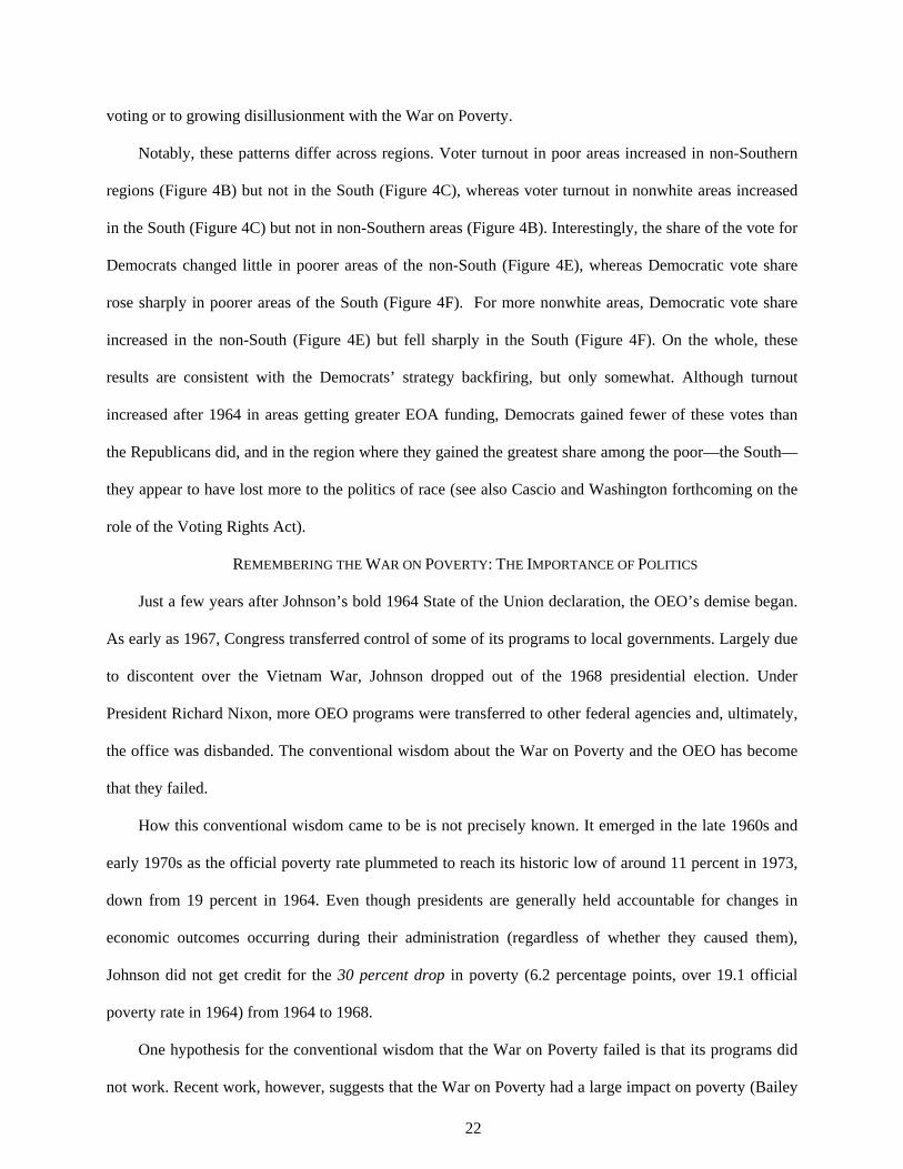
Table 2 presents the regression results. For brevity, tables 2 and 3 suppress the point estimates for the

covariates in X (the full set of estimates is reported in Appendix A). Huber-White standard errors are

presented in brackets beneath each estimate. The first three columns present the point estimates of

different metrics of county-level poverty rates and column 4 uses the share of the county population that

is nonwhite. Column 5 adds the political variables. Columns 6 to 8 present the estimates with all of the

variables combined using each of three poverty rates (the three measures are highly collinear, so they are

not included together).

These results provide strong evidence that the Johnson administration used OEO funding to fight

poverty. Within states where the poverty index did not bind, the population share in poverty (by three

measures) and share nonwhite are individually statistically significant at the 1 percent level and robust to

the inclusion of other covariates in columns 6 through 8. But the effects are not large in an economic

sense. A one standard-deviation higher share of the 1960 population in households with incomes less than

$3,000 (0.16) implies a $7.86 increase in real, cumulative per capita federal CAP funding—about one-

fifth of a standard deviation in funding (column 6). The implied elasticities are similar for measures of the

intensity of poverty. For a one standard deviation higher share of the 1960 population in households with

incomes less than $1,000 and $2,000, columns 6 and 7 imply a similar increase in cumulative per capita

federal CAP funding—0.14 and 0.17 of a standard deviation, respectively. By this metric, the population

share of nonwhites, however, is about twice as economically important. A one standard-deviation higher

share of nonwhites (0.16) implies a $14 increase in real, cumulative per capita federal CAP funding—

over one-third of a standard deviation in the dependent variable (columns 6 to 8).

Political considerations also shaped decisions at the OEO. A one standard-deviation increase in

23 A further source was Price Fishback, Michael Haines, and Paul Rhode, “Data Entered from the Agricultural Censuses of 1930, 1935, and 1940,” personal communication, 20 June 2012. The final version of these data are included in Haines (2010). Paternalism is difficult to measure with existing data, so we experiment with multiple measures of Southern plantation agriculture. Qualitatively similar results were derived by using an indicator variable based either on counties considered plantation areas, according to a special U.S. census report on 1910 cotton farming (U.S. Bureau of the Census 1916; Whatley 1987), or on the devolution of the plantation system, using sharecropping rates in 1959 (U.S. Bureau of the Census 1959; Haines 2010) to determine the percentage of sharecroppers among farm operators. Alston and Ferrie’s hypothesis also bears on the interpretation of variables for whether Democratic power on key committees in the House of Representatives is negatively correlated with CAP spending in the South, although we described these variables as part of P.

19

Democratic share in the 1964 presidential election has roughly the same effect as a one standard-deviation

increase in poverty—about 0.16 of a standard deviation increase in funding. Not only did more

Democratic counties receive more money per capita, funds also rewarded districts with larger increases in

Democratic share in the presidential elections between 1960 and 1964, with a one standard-deviation

increase in this variable leading to 0.20 of a standard deviation increase in funding. Whereas swing

counties received less funding, swing counties won by Democrats received slightly more ceteris paribus.

These findings are robust to the inclusion of identical covariates for the 1960 presidential election as well

as to alternative definitions of “swing” areas. In short, the Johnson administration invested in its new

Democratic constituency by directing OEO funds to Democrat-trending areas as well as to Democratic

strongholds. In contrast, we find no evidence that congressional committee membership during the 89th

Congress mattered at all (the results for the 88th and 90th Congress do not alter this conclusion). Counties

with representatives on major House committees, chairing major committees, or in positions of leadership

(Democratic or Republican) have no predictive power in any of our regressions.

Presidential politics, however, explains very little of county-level OEO’s funding decisions. To make

the relative contributions of poverty and politics more explicit, we summarize the partial R2 values of

these sets of variables at the bottom of Table 2—a simple metric for determining how much of the

variation in within-state per capita CAP funding is explained by the set of poverty variables or the set of

political variables.24 The R2 value for the political variables is 0.004 (column 5), significantly lower than

for the poverty variables. Across specifications, approximately 3 percent of the variation in funding is

explained by poverty, or 30 percent of the variation explained by the model. Politics explains less than 1

percent in all cases.

Much of the history of the War on Poverty focuses on the South and its interaction with civil rights.

The majority of nonwhites lived in the South, and Table 2 shows that the nonwhite population share

played an important role in shaping OEO funding. Moreover, the paternalism hypothesis (Alston and

Ferrie 1993, 1999) suggests that local economic, demographic, and political considerations may have had

24 Note that the partial R2 statistics are calculated by leaving each individual or set of regressors out of the respective model. This approach may understate the explanatory power of the excluded regressor to the degree that it is correlated with the included regressors. We choose this approach because it is a more conservative approach to attribution.

20

different effects in the South. For both reasons, Table 3 splits our sample into non-Southern and Southern

counties, roughly partitioning the country into halves (46 percent of all counties are in the South).

The results highlight some similarities and differences between the regions: poverty rates and share

nonwhite have a strong and robust relationship to OEO spending. Similarly, changes in the share of a

county voting for Democrats also matters in both regions, although Democratic strongholds do not appear

to be rewarded in the South (where most places were Democratic strongholds). The economic

significance of each of these variables, however, is weaker in the South. A one standard-deviation

increase in Southern poverty rates or share nonwhite implies a 0.12 and 0.11 standard deviation increase

in EOA spending, respectively (column 4). This is one-half (for poverty) to one-fifth (for share nonwhite)

the magnitude of these effects in the rest of the United States (column 1).

The results also reveal striking differences in funding patterns between the two regions. First,

roughly 40 percent of the variation in per capita OEO funding is explained by the model in non-Southern

regions (partial R2, columns 1 to 3). In the South, less than 3 percent is explained by the model (columns

4 to 6). Second, the lion’s share of the explained variation outside the South is accounted for by the

poverty variables (25 to 27 percent), whereas in the South very little of the variation is explained by

poverty measures (less than 1 percent in all cases). Third, presidential politics seem to matter very little in

general and even less in the South. Putting aside the fact that these estimates are statistically insignificant,

their magnitude in the South is half the size of the implied effects elsewhere.

Correlations of OEO Spending with Electoral Outcomes

Our final analysis investigates whether EOA money was successful in building the Democratic

coalition. Our analysis draws upon estimates by Jerome Clubb, William Flanigan, and Nancy Zingale

(2006) of House election voter turnout and share of votes for Democrats by county using a panel version

of equation (2) which omits the political variables and includes state-by-year fixed effects,

3 ∑ 1 , , ,

where is now voter turnout or share of votes cast for Democratic candidates in county i, in year

t=1950, 1952,…, 1958, 1962,…, 1972 (note: 1960 is omitted); are county fixed effects; , are

state-by-year fixed effects; and other variables remain as previously defined. The specifications describe

21

changes in voter turnout and support of Democrats in poorer and more nonwhite counties after accounting

for secular changes in state politics, redistricting in the state-by-year fixed effects, and the time-varying

effects of other covariates.

Figure 4 supports the claim that OEO spending boosted voter turnout (panel A) and support of the

Democrats (panel D) in poor areas. Panel A plots the point estimates for each year on the interaction

between year and either (1) the share of the population in households earning less than $3,000 per year

(solid line) or (2) the share nonwhite (dashed line). Except for a short-term increase in 1958, the

relationship of share nonwhite (dashed line) to voter turnout is stable from 1950 to 1962. In 1964,

however, the relationship increases rapidly. Counties with a one percentage point higher share nonwhite

in 1960 experienced a 0.20 percentage point increase in voter turnout during the 1968 election—a pattern

driven by higher turnout in nonwhite counties of the South. A more modest and short-run relationship is

seen for poorer counties, which experienced low turnout in 1960 and 1964 relative to the Eisenhower era,

only to surge to their highest level in 1966 before falling steadily from 1968 to 1972.

One interpretation of this result is that the groups the OEO intended to empower, especially

nonwhites, became more politically engaged during the 1960s. If this were the case, the share of voters

supporting Democrats should also grow in poorer and more nonwhite areas where turnout increased after

1964. But panel D shows this is only part of the story. After steadily decreasing during the 1950s and

early 1960s, support for Democrats in poorer areas increased from 1964 to 1968 (solid line). A one

standard-deviation higher poverty rate in 1960 (0.16) implies a 1.8 percentage point (11.3 x 0.16) higher

Democratic vote share in the 1966 election, or an increase of 3.5 percent. Because turnout was not

trending this way, the War on Poverty may have won over existing voters or changed the composition of

who went to the polls. The reverse appears to be true for more nonwhite areas. Again, after the 1950s and

early 1960s, when the relationship between nonwhite population share and share voting for Democrats

changed little, the Democratic vote share in areas that were more nonwhite decreased rapidly between

1964 and 1968. A one standard-deviation higher share nonwhite in 1960 (0.16) implies a 1.4 percentage

point (8.7 x 0.16) or 2.8 percent lower vote share in the 1968 election. The rising turnout in more

nonwhite counties, therefore, reflected increases in votes for Republicans. This is consistent with backlash

22

voting or to growing disillusionment with the War on Poverty.

Notably, these patterns differ across regions. Voter turnout in poor areas increased in non-Southern

regions (Figure 4B) but not in the South (Figure 4C), whereas voter turnout in nonwhite areas increased

in the South (Figure 4C) but not in non-Southern areas (Figure 4B). Interestingly, the share of the vote for

Democrats changed little in poorer areas of the non-South (Figure 4E), whereas Democratic vote share

rose sharply in poorer areas of the South (Figure 4F). For more nonwhite areas, Democratic vote share

increased in the non-South (Figure 4E) but fell sharply in the South (Figure 4F). On the whole, these

results are consistent with the Democrats’ strategy backfiring, but only somewhat. Although turnout

increased after 1964 in areas getting greater EOA funding, Democrats gained fewer of these votes than

the Republicans did, and in the region where they gained the greatest share among the poor—the South—

they appear to have lost more to the politics of race (see also Cascio and Washington forthcoming on the

role of the Voting Rights Act).

REMEMBERING THE WAR ON POVERTY: THE IMPORTANCE OF POLITICS

Just a few years after Johnson’s bold 1964 State of the Union declaration, the OEO’s demise began.

As early as 1967, Congress transferred control of some of its programs to local governments. Largely due

to discontent over the Vietnam War, Johnson dropped out of the 1968 presidential election. Under

President Richard Nixon, more OEO programs were transferred to other federal agencies and, ultimately,

the office was disbanded. The conventional wisdom about the War on Poverty and the OEO has become

that they failed.

How this conventional wisdom came to be is not precisely known. It emerged in the late 1960s and

early 1970s as the official poverty rate plummeted to reach its historic low of around 11 percent in 1973,

down from 19 percent in 1964. Even though presidents are generally held accountable for changes in

economic outcomes occurring during their administration (regardless of whether they caused them),

Johnson did not get credit for the 30 percent drop in poverty (6.2 percentage points, over 19.1 official

poverty rate in 1964) from 1964 to 1968.

One hypothesis for the conventional wisdom that the War on Poverty failed is that its programs did

not work. Recent work, however, suggests that the War on Poverty had a large impact on poverty (Bailey

23

and Danziger 2013). Some of this effect was immediate. Recent work extending the supplemental poverty

measure (which takes a fuller accounting of changes in non-cash transfers and those through the tax code)

backwards in time shows that poverty rates fell from almost 26 percent in 1967 to 16 percent today, a fall

greatly aided by programs begun under the War on Poverty (Wimer et al. 2013). A complementary,

consumption-based measure of poverty registers a 26 percentage point decline from 1960 to 2010, with

just over two-thirds of this decline occurring before 1980 (Meyer and Sullivan 2012). Many benefits

were also longer-run in nature: a growing literature argues that many War on Poverty programs were

fairly successful at increasing human capital, improving health, and reducing racial inequality over the

longer term (Ludwig and Miller 2007; Chay et al. 2010; Cascio et al. 2010; Almond et al. 2011; Bailey

2012; Gillezeau 2012; Bailey and Goodman-Bacon 2012; Bailey 2013; Cunningham 2013; Almond et al.

forthcoming). It is puzzling that the Johnson administration did not get credit for some of these successes.

A second hypothesis is that the “failure” narrative reflects the success of critics in rewriting history.

But this claim forgets the fact that President Ronald Reagan’s quip in his 1988 State of the Union that

“the federal government fought the war on poverty, and poverty won” was not new. Allegations of the

War on Poverty’s failure dates to critics in both political parties. Accounts from the late 1960s argued

that the CAP programs were born of conflicting ideas and administrative chaos—the programs of

professors, not practitioners (Levine 1970; Forget 2011).25 Prominent scholars agreed saying that the War

on Poverty’s “promises were extreme; the specific remedial actions were untried and untested; [and] the

finances were grossly inadequate” (Ginzberg and Solow 1974, p. 219).

The difference in historical memory of the War on Poverty and the New Deal is striking. Although

the New Deal’s effectiveness as a set of policies has been contested in scholarship, its policies—even

without a large or immediate rebound in private sector employment—were regarded as successful at the

time as they are remembered today. This collective memory of the New Deal’s success transcends party

lines. When criticized for dismantling New Deal programs, Reagan corrected reporters noting he had

voted for Roosevelt four times and remarked, “I’m trying to undo the Great Society…it was LBJ’s war on

25 Moynihan, Daniel Patrick. “The Professors and the Poor.” Commentary, August 1968. Other critics argued that not enough money was spent on the poor and that the Johnson administration did too little to effect change (King 1968; Katznelson 1989).

24

poverty that led us to our present mess” (Berkowitz 2001, p. 98). Although the Great Depression lasted,

Roosevelt’s New Deal programs are remembered as successes.

This paper’s analysis provides hints regarding a third hypothesis for the belief that the War on

Poverty failed: implementation. Our finding that the Johnson administration distributed CAP funds to

poorer areas—rather than those with greater political importance—shows how differently the War on

Poverty was waged than the New Deal. Rather than including and empowering state and local politicians

and community leaders in the allocation process as in the New Deal, OEO funds were used to circumvent

and challenge these interests. OEO funds flowed to poor and nonwhite areas, which empowered new

constituencies of poor and African Americans. Our quantitative analysis underscores these differences.

Measured by partial R2, Fishback, Kantor, and Wallis’s (2003) political variables explain 25 percent of

the county-level distribution of New Deal spending. The equivalent variables during the War on Poverty

explain roughly one percent of the variation in OEO county-level spending (see Appendix A Table A5).

Unlike New Deal funding, OEO grants did not flow to (or away from) areas with powerful

congresspersons or meaningfully reward swing voters that helped Democrats win the most liberal

Congress since the New Deal.

In line with many contemporary accounts and retrospectives, our analysis suggests that OEO funding

generated backlash and appeared to hurt Democrats in the late 1960s and early 1970s—especially relating

to the politics of race in the South. Unlike the New Deal, which engendered good will for decades, the

War on Poverty generated resentments—and, in the shorter term, votes for Republicans in areas with

more potential African American voters.

Given Johnson’s ambition to recreate Roosevelt’s style and political reputation, the differences

between the political economy of the New Deal and War and Poverty are perhaps surprising. But just

days after Kennedy’s assassination, a staffer advised Johnson to focus on small, popular policy proposals

instead of bold—and divisive—goals like civil rights. Johnson responded, “What the hell’s the presidency

for?” (Caro 2012, p. 428). The OEO’s focus on fighting poverty and racial discrimination—over politics

as usual—is consistent with this humanitarian vision. The quantitative picture that emerges from our

analysis is that the War on Poverty was a sincere attempt, albeit an underfunded one, to champion change.

24

REFERENCES

Adler, E. Scott. “Congressional District Data File, 88th Congress.” University of Colorado, Boulder, CO. Accessed May 2013. [http://sobek.colorado.edu/~esadler/Congressional_District_Data.html].

Almond, Douglas, Hilary W. Hoynes, and Diane Whitmore Schanzenbach. “Inside the War on Poverty: The Impact of Food Stamps on Birth Outcomes.” Review of Economics and Statistics 93, no. 2 (2011): 387-403.

Almond, Douglas, Kenneth Chay, and Michael Greenstone. “Civil Rights, the War on Poverty, and Black-White Convergence in Infant Mortality in the Rural South and Mississippi.” American Economic Review, forthcoming.

Alston, Lee J., and Joseph P. Ferrie. “Paternalism in Agricultural Labor Contracts in the U.S. South: Implications for the Growth of the Welfare State.” American Economic Review 83, no. 4 (1993): 852-76.

__________. Southern Paternalism and the American Welfare State: Economics, Politics, and the Institutions in the South, 1865-1965. Cambridge: Cambridge University Press, 1999.

Anderson, Gary M., and Robert D. Tollison. “Congressional Influence and Patterns of New Deal Spending, 1933-1939.” Journal of Law and Economics 34, no. 1 (1991): 161-75.

Bailey, Martha J., “Reexamining the Impact of Family Planning Programs on U.S. Fertility: Evidence from the War on Poverty and Early Years of Title X.” American Economic Journal: Applied Economics 4, no. 2 (2012): 62-97.

__________. “Fifty Years of U.S. Family Planning: Evidence on the Long-Run Effects of Increasing Access to Contraception.” Brookings Papers on Economic Activity, Fall 2013.

__________ and Sheldon Danziger, eds. Legacies of the War on Poverty. New York: Russell Sage Foundation, 2013.

__________ and Andrew Goodman-Bacon. “The War on Poverty’s Experiment in Public Medicine: The Impact of Community Health Centers on the Mortality of Older Americans.” Working paper, University of Michigan, Ann Arbor, MI, June 2012.

Berkowitz, Edward. “Losing Ground? The Great Society in Historical Perspective.” In The Columbia Guide to America in the 1960s, edited by D. Farber and B. Bailey, 98-108. New York: Columbia University Press, 2001.

Caro, Robert A. The Path to Power. New York: Alfred A. Knopf, 1982. __________. Master of the Senate. New York: Alfred A. Knopf, 2002. __________. The Passage of Power. New York: Alfred A. Knopf, 2012. Carter, David. The Music Has Gone Out of the Movement: Civil Rights and the Johnson Administration, 1965-1968.

Chapel Hill, NC: University of North Carolina Press, 2009. Cascio, Elizabeth, and Ebonya Washington. “Valuing the vote: The Redistribution of Voting Rights and State Funds

Following the Voting Rights Act of 1965.” Quarterly Journal of Economics 129, no. 1 (2014): 376-433. Cascio, Elizabeth, Nora Gordon, Ethan Lewis, et al. “Paying for Progress: Conditional Grants and the Desegregation

of Southern Schools.” Quarterly Journal of Economics 125, no. 1 (2010): 445-82. Chay, Kenneth Y., Daeho Kim, and Shailender Swarminathan. “Medicare, Hospital Utilization and Mortality:

Evidence from the Program’s Origins.” Working paper, Brown University, Providence, RI, 2010. http://www.chicagofed.org/digital_assets/others/events/2010/health_care_conference/paper_chay.pdf (accessed 8 August 2013).

Clubb, Jerome M., William H. Flanigan, and Nancy H. Zingale. “Electoral Data for Counties in the United States: Presidential and Congressional Races, 1840-1972.” ICPSR08611-v1. Ann Arbor, MI: Inter-university Consortium for Political and Social Research [producer and distributor], 13 November 2006.

Collins, William J., and Robert A. Margo. “The Economic Aftermath of the 1960s Riots in American Cities: Evidence from Property Values.” Journal of Economic History 67, no. 4 (2007): 849-83.

Commentary, August 1968. Congressional Record, 88th Cong., 2nd sess., 1964a, Vol. 110, pt. 7, 28 April. __________. 88th Cong., 2nd sess., 1964b, Vol. 110, pt. 13, 23 July. __________. 88th Cong., 2nd sess., 1964c, Vol. 110, pt. 14, 6 August. Congressional Quarterly Weekly Report. “Congress Clears Johnson’s Anti-Poverty Bill,” 14 August 1964a, pp.

1729–35. __________. “CQ Senate Votes 218 through 223,” 23 July 1964b, p. 1567. __________. “Senate Passes Johnson’s Anti-Poverty Bill, 61-34,” 23 July 1964c, pp. 1533–34. Congressional Quarterly Almanac, 1965. “Antipoverty Program Funds Doubled.” Washington, DC, pp. 405–20. Couch, Jim F., and William F. Shughart. The Political Economy of the New Deal. New York: Edward Elgar, 1998. Council of Economic Advisers. Economic Report of the President. Washington, DC: U.S. Government Printing

Office, 1964. Cunningham, Jamein. “More Lawyers, More Crime? The Impact of the OEO Legal Services Program on Crime.”

25

Working Paper, University of Michigan, Ann Arbor, MI, 2013. http://www-personal.umich.edu/~jamein/Lawyers_Crime.pdf (accessed 12/30/2013).

Davies, Gareth. From Opportunity to Entitlement: The Transformation and Decline of Great Society Liberalism. Lawrence: University Press of Kansas, 1996.

Depew, Briggs, Price Fishback, and Paul Rhode. “New Deal or No Deal in the Cotton South: The Effect of the AAA on the Agricultural Labor Structure.” Mimeo, University of Arizona, Tucson, AZ, 27 April 2012.

Fishback, Price. “The New Deal.” In Government and the American Economy, edited by Price Fishback et al., 384-430. Chicago: University of Chicago Press, 2007.

Fishback, Price V., Michael R. Haines, and Paul W. Rhode. “Data Entered from the Agricultural Censuses of 1930, 1935, and 1940.” Shared by personal correspondence, June 2012.

Fishback, Price, Shawn Kantor, and John Wallis. “Can the New Deal’s Three R’s Be Rehabilitated? A Program-by-Program, County-by-County Analysis.” Explorations in Economic History 40, no. 2 (2003): 278-307.

Fishback, Price, and John Wallis. “What Was New about the New Deal?” In The Great Depression of the 1930s: Lessons for Today, edited by Nicolas Crafts and Peter Fearon, 291-327. Oxford, UK: Oxford University Press, 2012.

Fleck, Robert K. “Population, Land, Economic Conditions, and the Allocation of New Deal Spending.” Explorations in Economic History 38, no. 2 (2001): 296-304.

__________. “Voter Influence and Big Policy Change: The Positive Political Economy of the New Deal.” Journal of Political Economy 116, no. 1 (2008): 1-37.

Forget, Evelyn L. “A Tale of Two Communities: Fighting Poverty in the Great Society (1964-68).” History of Political Economy 43, no. 1 (2011): 199-223.

Galbraith, John Kenneth. The Affluent Society. New York: Houghton Mifflin, 1958. Germany, Kent B. New Orleans after the Promises: Poverty, Citizenship, and the Search for the Great Society.

Athens, GA: University of Georgia Press, 2007. Gettleman, Marvin E., and David Mermelstein. “Sargent Shriver to the House Subcommittee on the War on Poverty,

April 12 1965.” In The Great Society Reader: The Failure of American Liberalism, edited by Marvin E. Gettleman and David Mermelstein. New York: Random House, 1966.

Gillette, Michael L. Launching the War on Poverty: An Oral History. New York: Twayne Publishers, 1996. Gillezeau, Rob. “Did the War on Poverty Cause Race Riots?” Mimeo, University of Michigan, Ann Arbor, MI,

November 2012. Ginzberg, Eli, and Robert M. Solow. The Great Society: Lessons for the Future. New York: Basic Books, 1974. Haines, Michael R., and Inter-university Consortium for Political and Social Research. Historical, Demographic,

Economic, and Social Data: The United States, 1790-2002. ICPSR02896-v3. Ann Arbor, MI: Inter-university Consortium for Political and Social Research [distributor], 2010-05-21. doi:10.3886/ICPSR02896.v3.

Harper’s Magazine, December 1965. Harrington, Michael. The Other America. New York: Penguin, 1962. Heller, Walter F. “Oral History Interview 1, February 20.” Austin, TX: Lyndon Baines Johnson Library, 1970. Inter-university Consortium for Political and Social Research, and Congressional Quarterly, Inc. United States

Congressional Roll Call Voting Records, 1789-1998. ICPSR00004-v3. Ann Arbor, MI: Inter-university Consortium for Political and Social Research [distributor], 2010-05-06. doi:10.3886/ICPSR00004.v3.

Johnson, Lyndon B. “Annual Message to Congress on the State of the Union, January 8, 1964.” In Public Papers of the Presidents of the United States: Lyndon B. Johnson, 1963-1964. Vol. I, 112-17. Washington, DC: GPO, 1965.

Jordan, Barbara C., and Elspeth D. Rostow. The Great Society: A Twenty Year Critique. Austin, TX: Lyndon Baines Johnson Library / Lyndon Baines Johnson School of Public Affairs, 1986.

Katznelson, Ira. Fear Itself: The New Deal and the Origins of Our Time. New York: Liveright Publishing Corporation (2013).

Katznelson, Ira. “Was the Great Society a Lost Opportunity?” In The Rise and Fall of the New Deal Order: 1930-1980, edited by Steve Fraser and Gary Gerstle, 185-211. Princeton: Princeton University Press, 1989.

King, Jr., Martin Luther. Where Do We Go from Here: Chaos or Community? Boston: Beacon Press, 1968. Levine, Robert A. The Poor Ye Need Not Have with You: Lessons from the War on Poverty. Cambridge: MIT Press,

1970. Levitan, Sar A. The Great Society’s Poor Law: A New Approach to Poverty. Baltimore: Johns Hopkins Press, 1969. Ludwig, Jens, and Douglas L. Miller. “Does Head Start Improve Children’s Life Chances? Evidence from a

Regression Discontinuity Design.” Quarterly Journal of Economics 122, no. 1 (2007): 159-208. McKee, Guian A. “‘This Government Is with Us’: Lyndon Johnson and the Grassroots War on Poverty.” In The War

on Poverty: A New Grassroots History 1964-1980, edited by Annelise Orleck and Lisa Gayle Hazirjian, 31-62. Athens, GA: University of Georgia Press, 2011.

26

__________. Lyndon B. Johnson and the War on Poverty: Introduction to the Digital Edition. Charlottesville, VA: University of Virginia, 2010. http://rotunda.upress.virginia.edu/pdf/american-cent/WarOnPoverty-introduction-USletter.pdf (accessed 24 June 2012).

Meyer, Bruce, and James X. Sullivan. “Winning the War: Poverty from the Great Society to the Great Recession.” Brookings Papers on Economic Activity, Fall 2012: 133-200.

Miller Center, University of Virginia. Presidential Recordings Program. 6216 - Joseph Clark (WH6411.07) [audio recording], 1964. http://millercenter.org/scripps/archive/presidentialrecordings (accessed June 2012).

National Archives Records about Community Action Program Grants and Grantees (NACAP). [Electronic Records]; Grantee Organization Masterfile, 7/1/1964-6/30/1971; Grantee Organization Master File, 7/1/1971 - 9/30/1981; Funded Program Account Master File, 7/1/1964 - 6/30/1971; Funded Program Account Master File, 7/1/1971 - 9/30/1977; Funded Program Account Master File, 10/1/1977 - 9/30/1981; Record Group 381 (National Archives at College Park: College Park MD).

New Republic, 28 March 1964. New York Times, various dates. Newman, Katherine S., and Rourke L. O’Brien. Taxing the Poor. Berkeley, CA: University of California Press,

2011. O’Connor, Alice. Poverty Knowledge: Social Science, Social Policy, and the Poor in Twentieth-Century U.S.

History. Princeton, NJ: Princeton University Press, 2001. Office of Economic Opportunity. Annual Reports. Washington, DC: GPO, 1965-1968. Oregon Center for Public Policy. “How We Measure Poverty.” February 2000.

http://www.ocpp.org/poverty/how.htm (accessed June 2012). Orleck, Annelise, and Lisa Gayle Hazirjian, eds. The War on Poverty: A New Grassroots History 1964-1980.

Athens, Georgia: University of Georgia Press, 2011. Reagan, Ronald. “Address Before a Joint Session of Congress on the State of the Union, January 25, 1988.” Online

by Gerhard Peters and John T. Woolley, The American Presidency Project at http://www.presidency.ucsb.edu/ws/?pid=36035 (accessed August 17, 2013).

Schlesinger, Arthur Jr. A Thousand Days: John F. Kennedy in the White House. Boston, MA: Houghton Mifflin, 1965.

U.S. Bureau of the Census. Plantation Farming in the United States. Washington, DC: GPO, 1916. __________. Census of Agriculture. Washington, DC: GPO, 1930 and 1935. __________. Census of Agriculture. Washington, DC: GPO, 1959. __________. Census of Government: 1962. Vol. VII (Hol Doc C 3.145/4 1962). Washington, DC: GPO, 1964. U.S. Department of Defense. Office of the Under Secretary of Defense for Personnel and Readiness. “Vietnam

Conflict Extract Data File.” Series: Defense Casualty Analysis System (DCAS) Extract Files. Record Group 330: Records of the Office of the Secretary of Defense. National Archives at College Park, Maryland, 2008 (retrieved from the Access to Archival Databases at www.archives.gov).

U.S. Department of Labor. Manpower Report of the President. Washington, DC: GPO, 1965-1968. U.S. Department of Health, Education and Welfare. Social Security Bulletin Annual Statistical Supplement.

Washington, DC: GPO, 1965-1968. U.S. House of Representatives Committee on Education and Labor. Hearings before the Subcommittee on the War

on Poverty Program on H.R. 10440. 88th Cong., 2nd sess., 1964a. __________. Committee on Education and Labor. Report [to Accompany H.R. 11377] (H.R. Report 88-1458) 88th

Cong., 2nd sess., 1964b. __________. Conference Report: Economic Opportunity Amendments of 1967 [to accompany S. 2388] (H.R. Report

90-1012). 90th Cong., 1st sess., 1967. Wall Street Journal, 29 April 1964. Wallis, John J. “The Birth of the Old Federalism: Financing the New Deal, 1932-1940.” Journal of Economic

History 44, no. 1 (1984): 139-59. __________. “Employment, Politics, and Economic Recovery during the Great Depression.” Review of Economics

and Statistics 59, no. 3 (1987): 516-20. __________. “The Political Economy of New Deal Spending Revisited, Again: With and without Nevada.”

Explorations in Economic History 35, no. 2 (1998): 140-70. __________. “The Political Economy of New Deal Spending, Yet Again: A Reply to Fleck.” Explorations in

Economic History 38, no. 2 (2001): 305-14. Whatley, Warren. “Southern Agrarian Labor Contracts as Impediments to Cotton Mechanization.” Journal of

Economic History 47, no. 1 (1987): 45-70. Wimer, Christopher, Liana Fox, Irv Garfinkel, Neeraj Kaushal, and Jane Waldfogel. “Trends in Poverty with an

Anchored Supplemental Poverty Measure.” Mimeo Columbia University released December 5, 2013.

27

http://socialwork.columbia.edu/sites/default/files/file_manager/pdfs/News/Anchored%20SPM.December7.pdf (accessed January 19, 2014).

Wright, Gavin. “The Political Economy of New Deal Spending.” Review of Economics and Statistics 56, no. 1 (1974): 30-38.

28

Table 1. The Relationship between EOA Poverty Index and CAP Spending, 1965 to 1968 (1) (2) (3) (4) (5)

A. Dependent Variable: Real Federal CAP Funding (No Census Region Fixed Effects) 1965 1966 1967 1968 1965-1968 Index apportioned funds in FY

0.898*** 1.137*** 1.395*** 1.190*** [0.137] [0.0915] [0.0563] [0.0362]

Cumulative apportioned funds, 1965-1968 1.206*** [0.0549]

Constant -1.002** -0.373 -0.495 1.015 -1.16 [0.476] [0.876] [0.708] [0.680] [2.408] Observations 48 48 48 48 48 R2 0.763 0.914 0.93 0.92 0.932 Coefficient >1 p-value 0.230 0.070 0.000 0.000 0.000 Coefficient=1.25 p-value 0.033 0.497 0.001 0.790 0.914

B. Dependent Variable: Real Federal CAP Funding (With Census Region Fixed Effects) 1965 1966 1967 1968 1965-1968 Index apportioned funds in FY

0.938*** 1.168*** 1.418*** 1.201*** [0.103] [0.0724] [0.0366] [0.0372]

Cumulative apportioned funds, 1965-1968 1.230*** [0.0340]

Midwest=1 -1.470* 0.654 -2.756* -1.841 -5.591 [0.734] [1.268] [1.397] [1.247] [4.028] South=1 -3.339*** -0.999 -4.486** -1.53 -10.90** [0.925] [1.464] [1.800] [1.888] [5.183] West=1 -0.201 3.297* 0.572 1.548 5.699 [0.695] [1.683] [1.322] [1.454] [4.493] Constant 0.346 -1.295 1.285 1.479* 1.542 [0.448] [1.150] [0.988] [0.861] [2.738] Observations 48 48 48 48 48 R2 0.862 0.93 0.945 0.927 0.946 Coefficient >1 p-value 0.274 0.013 0.000 0.000 0.000 Coefficient=1.25 p-value 0.014 0.659 0.000 0.970 0.386

Notes: Stars denote statistical significance as follows: * = Significant at the 5 percent level. ** = Significant at the 1 percent level. *** = Significant at the .05 percent level. Huber-White standard errors are in brackets. Sample excludes Alaska, Hawaii, and the District of Columbia. Sources: See Figure 1.

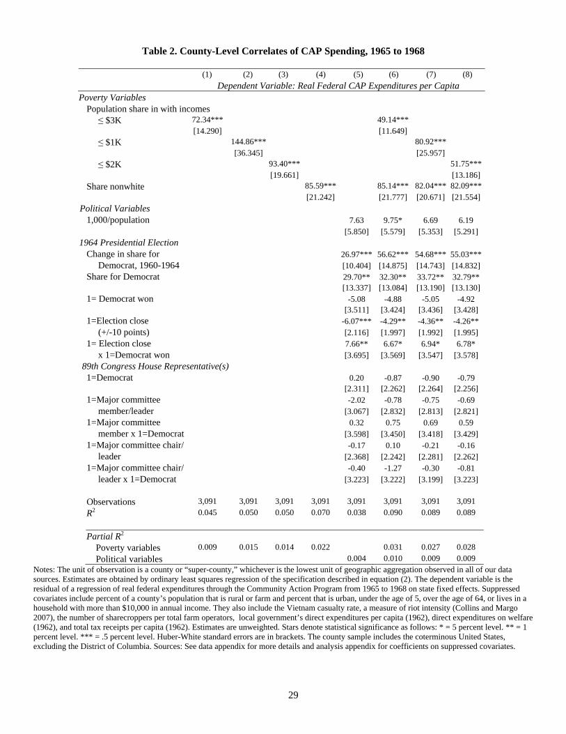
29

Table 2. County-Level Correlates of CAP Spending, 1965 to 1968

(1) (2) (3) (4) (5) (6) (7) (8)

Dependent Variable: Real Federal CAP Expenditures per Capita Poverty Variables

Population share in with incomes ≤ $3K 72.34*** 49.14***

[14.290] [11.649]

≤ $1K 144.86*** 80.92***

[36.345] [25.957]

≤ $2K 93.40*** 51.75***

[19.661] [13.186]

Share nonwhite 85.59*** 85.14*** 82.04*** 82.09***

[21.242] [21.777] [20.671] [21.554]

Political Variables

1,000/population 7.63 9.75* 6.69 6.19 [5.850] [5.579] [5.353] [5.291]

1964 Presidential Election Change in share for 26.97*** 56.62*** 54.68*** 55.03*** Democrat, 1960-1964 [10.404] [14.875] [14.743] [14.832]Share for Democrat 29.70** 32.30** 33.72** 32.79** [13.337] [13.084] [13.190] [13.130]1= Democrat won -5.08 -4.88 -5.05 -4.92 [3.511] [3.424] [3.436] [3.428] 1=Election close -6.07*** -4.29** -4.36** -4.26** (+/-10 points) [2.116] [1.997] [1.992] [1.995] 1= Election close 7.66** 6.67* 6.94* 6.78* x 1=Democrat won [3.695] [3.569] [3.547] [3.578]

89th Congress House Representative(s) 1=Democrat 0.20 -0.87 -0.90 -0.79 [2.311] [2.262] [2.264] [2.256] 1=Major committee -2.02 -0.78 -0.75 -0.69 member/leader [3.067] [2.832] [2.813] [2.821] 1=Major committee 0.32 0.75 0.69 0.59 member x 1=Democrat [3.598] [3.450] [3.418] [3.429] 1=Major committee chair/ -0.17 0.10 -0.21 -0.16 leader [2.368] [2.242] [2.281] [2.262] 1=Major committee chair/ -0.40 -1.27 -0.30 -0.81 leader x 1=Democrat [3.223] [3.222] [3.199] [3.223]

Observations 3,091 3,091 3,091 3,091 3,091 3,091 3,091 3,091

R2 0.045 0.050 0.050 0.070 0.038 0.090 0.089 0.089

Partial R2

Poverty variables 0.009 0.015 0.014 0.022 0.031 0.027 0.028

Political variables 0.004 0.010 0.009 0.009 Notes: The unit of observation is a county or “super-county,” whichever is the lowest unit of geographic aggregation observed in all of our data sources. Estimates are obtained by ordinary least squares regression of the specification described in equation (2). The dependent variable is the residual of a regression of real federal expenditures through the Community Action Program from 1965 to 1968 on state fixed effects. Suppressed covariates include percent of a county’s population that is rural or farm and percent that is urban, under the age of 5, over the age of 64, or lives in a household with more than $10,000 in annual income. They also include the Vietnam casualty rate, a measure of riot intensity (Collins and Margo 2007), the number of sharecroppers per total farm operators, local government’s direct expenditures per capita (1962), direct expenditures on welfare (1962), and total tax receipts per capita (1962). Estimates are unweighted. Stars denote statistical significance as follows: * = 5 percent level. ** = 1 percent level. *** = .5 percent level. Huber-White standard errors are in brackets. The county sample includes the coterminous United States, excluding the District of Columbia. Sources: See data appendix for more details and analysis appendix for coefficients on suppressed covariates.

30

Table 3. County-Level Correlates of CAP Spending in the South and Non-South, 1965 to 1968

(1) (2) (3) (4) (5) (6)

Dependent Variable: Real Federal CAP Expenditures per Capita Non-South Only South Only Poverty Variables Population share with incomes

≤ $3K 83.45*** 31.93**

[26.025] [12.451]

≤ $1K 211.44*** 45.54** [70.400] [20.150] ≤ $2K 127.09*** 34.39*** [37.551] [12.256] Share nonwhite 411.66*** 396.67*** 396.04*** 21.65* 20.18* 19.45 [88.228] [81.937] [85.550] [12.375] [11.710] [11.972] Political Variables

1,000/population 7.75 2.69 2.84 1.39 0.36 -0.85 [8.332] [8.355] [8.818] [2.974] [3.030] [3.195] 1964 Presidential Election Change in share for 45.86** 45.01** 42.77** 33.04** 31.83** 31.93** Democrat, 1960-1964 [20.882] [21.264] [21.223] [13.342] [13.390] [13.405] Share for Democrat 51.78** 53.59** 53.19** 1.69 2.27 1.96 [22.044] [22.018] [22.090] [14.422] [14.373] [14.384] 1= Democrat won -9.11* -9.08* -9.00* 1.26 1.17 1.25 [5.073] [5.085] [5.064] [4.337] [4.337] [4.334] 1=Election close -3.48 -3.83 -3.33 -2.37 -2.40 -2.37 (+/-10 points) [2.965] [3.049] [3.012] [2.317] [2.343] [2.314] 1= Election close 9.23* 10.05** 9.30* 2.72 2.66 2.76 x 1=Democrat won [4.735] [4.764] [4.746] [4.480] [4.500] [4.487] 89th Congress House Representative(s)

1=Democrat -1.97 -2.24 -2.02 2.54 2.60 2.82 [2.251] [2.229] [2.243] [3.519] [3.561] [3.554] 1=Major committee 3.26 3.41 3.48 -6.09 -6.27 -6.08 member/leader [2.791] [2.770] [2.766] [3.897] [3.876] [3.892] 1=Major committee member -3.68 -4.26 -4.16 4.39 4.54 4.31 x 1=Democrat [3.529] [3.489] [3.507] [3.920] [3.929] [3.930] 1=Major committee chair/ -2.68 -2.75 -2.58 -0.12 0.41 0.13 leader [3.038] [3.030] [3.045] [2.813] [2.785] [2.796] 1=Major committee chair/ 20.37* 19.49* 20.35* leader x 1=Democrat [10.742] [10.478] [10.481]

Observations 1,677 1,677 1,677 1,414 1,414 1,414 R2 0.413 0.419 0.417 0.028 0.027 0.028

Partial R2

Poverty variables 0.279 0.253 0.252 0.006 0.005 0.006

Political variables 0.022 0.024 0.023 0.005 0.004 0.004 Notes: See Table 2 notes for specification and other details. In columns 4-6, interactions of 1=Represented by a House Democrat with committee membership and chairmanship/leadership are omitted due to collinearity. Sources: See data appendix for more details.

31

Figure 1. The Relationship of 1965-1968 CAP Spending to the EOA Apportionment Index, by Fiscal Year

A. Fiscal Year 1965 B. Fiscal Year 1966

C. Fiscal Year 1967 D. Fiscal Year 1968

Notes: The x-axis indicates the total minimum funding according to the EOA poverty index for each state for the relevant fiscal year in millions of 1968 dollars. See equation (1) and the text for details. The y-axis indicates actual federal allocations in millions of 1968 dollars for each state for the relevant fiscal year, including index allocations and the remaining 20 percent of CAP funds at Shriver’s discretion. The solid line is the 45-degree line, and the dashed line is fit by least squares regression. A state will fall along the 45-degree line if it received the minimum apportioned in the EOA. Points above the 45-degree line indicate that a state received more than its minimum apportionment, whereas points below the line indicate the reverse. Sources: EOA index is developed from U.S. House (1964b), U.S. Department of Labor (1965-1968), and U.S. Department of Health, Education, and Welfare (1965-1968). Actual allocations are aggregated using the NACAP grant data.

NVWYVTDENHIDMTNDSDUTME

RI

NE

NMOR

AZ

KSCOCT

IA

MD

WIWAIN

AROKMNWVVA

SC

MA

KYMO

NJ

FL

TNGA

MSLAAL

MI

NC

OH

IL

TX

PA

NY

CA

05

1015

20A

ctua

l CA

P A

lloc

atio

ns

0 5 10 15 20State Funding Per EOA Index

WYNVVTDENHIDNDMTSDUTRIMENE

NMOR

AZ

KSCOCT

IAMD

WIINWA

AROKMNWVVASC

MA

FLKYNJ

TN

MO

MS

GA

LAAL

MI

NC

OH

IL

PA

TX

NY

CA

020

4060

80A

ctua

l CA

P A

lloc

atio

ns

0 20 40 60State Funding Per EOA Index

WYNHVTNVDEIDMTNDSDUTRIMENE

NMOR

AZ

KS

COCT

IAMDWA

INWIMNAROKWVVASC

MAKYFLNJ

MO

TN

MS

GALAAL

MI

NCOH

ILPA TX

NY

CA

050

100

Act

ual C

AP

All

ocat

ions

0 20 40 60State Funding Per EOA Index

WYNHVTNVDEIDMTNDSDRIUTMENE

NM

KSOR

AZ

COCT

IA

WA

MDWIMN

INAROKWVVA

KY

SC

MAFLNJMO

TN

MS

LAGAAL

MINC

OH

IL

PA

TX

NY

CA

020

4060

80A

ctua

l CA

P A

lloc

atio

ns

0 20 40 60 80State Funding Per EOA Index

32

Figure 2. The Relationship of Cumulative 1965-1968 CAP Spending to the EOA Apportionment Index

Notes: The x-axis indicates the total minimum funding according to the EOA poverty index for each state for fiscal years 1965-1968 in millions of 1968 dollars. See equation (1) and the text for details. The y-axis indicates actual federal allocations in millions of 1968 dollars for each state, including index allocations and the remaining 20 percent of CAP funds at Shriver’s discretion. Sources: See Figure 1.

WYNHNVVTDEIDMTNDSDUTRIMENE

NMOR

AZ

KS

COCT

IAMDWAWIINMNAROKWVVASC

MAKYFLNJMO

TN

MS

GA

LAAL

MI

NC

OH

IL

PATX

NY

050

100

150

200

Act

ual C

AP

All

ocat

ions

0 50 100 150 200State Funding Per EOA Index

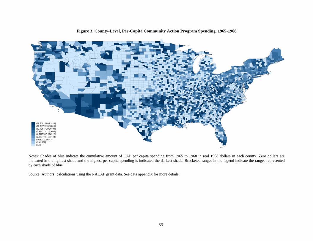
33

Figure 3. County-Level, Per-Capita Community Action Program Spending, 1965-1968

Notes: Shades of blue indicate the cumulative amount of CAP per capita spending from 1965 to 1968 in real 1968 dollars in each county. Zero dollars are indicated in the lightest shade and the highest per capita spending is indicated the darkest shade. Bracketed ranges in the legend indicate the ranges represented by each shade of blue. Source: Authors’ calculations using the NACAP grant data. See data appendix for more details.

34

Figure 4. County-Level Election Outcomes in the House of Representatives by Year and County Characteristics

A. Voter Turnout, All Counties

B. Voter Turnout, Non-South Only

C. Voter Turnout, South Only

-15

-5

5

15

25

35

1950 1952 1954 1956 1958 1960 1962 1964 1966 1968 1970 1972

Household Income < $3,000 / year Nonwhite Population

-30

-10

10

30

50

1950 1952 1954 1956 1958 1960 1962 1964 1966 1968 1970 1972

-20

-10

0

10

20

30

40

1950 1952 1954 1956 1958 1960 1962 1964 1966 1968 1970 1972

35

Figure 4 (continued)

D. Democratic Vote Share, All Counties

E. Democratic Vote Share, Non-South Only

F. Democratic Vote Share, South Only

Notes: Estimates plot the changing relationship of share of population in poverty and share of population nonwhite to the outcome variable of interest. The outcome variable for panels A, B, and C is voter turnout. For panels D, E, and F, the outcome variable is Democratic vote share. Smaller point lines mark pointwise 95-percent confidence intervals. See the text for more details. Sources: Estimated voter turnout and Democratic vote share from Clubb, Flanigan, and Zingale (2006). Household income <$3,000 and nonwhite shares from Haines (2010). See data appendix for more details.

-30

-10

10

30

1950 1952 1954 1956 1958 1960 1962 1964 1966 1968 1970 1972

Household Income < $3,000 / year Nonwhite Population

-40

-20

0

20

40

1950 1952 1954 1956 1958 1960 1962 1964 1966 1968 1970 1972

-50

-30

-10

10

30

50

1950 1952 1954 1956 1958 1960 1962 1964 1966 1968 1970 1972