How is Machine Learning Useful forMacroeconomic Forecasting?∗

Philippe Goulet Coulombe1† Maxime Leroux2 Dalibor Stevanovic2‡

Stéphane Surprenant2

1University of Pennsylvania2Université du Québec à Montréal

This version: February 28, 2019

Abstract

We move beyond Is Machine Learning Useful for Macroeconomic Forecasting? by addingthe how. The current forecasting literature has focused on matching specific variables andhorizons with a particularly successful algorithm. To the contrary, we study a wide rangeof horizons and variables and learn about the usefulness of the underlying features driv-ing ML gains over standard macroeconometric methods. We distinguish 4 so-called fea-tures (nonlinearities, regularization, cross-validation and alternative loss function) andstudy their behavior in both the data-rich and data-poor environments. To do so, wecarefully design a series of experiments that easily allow to identify the treatment effectsof interest. The simple evaluation framework is a fixed-effects regression that can be un-derstood as an extension of the Diebold and Mariano (1995) test. The regression setupprompt us to use a novel visualization technique for forecasting results that conveysall the relevant information in a digestible format. We conclude that (i) more data andnon-linearities are very useful for real variables at long horizons, (ii) the standard factormodel remains the best regularization, (iii) cross-validations are not all made equal (butK-fold is as good as BIC) and (iv) one should stick with the standard L2 loss.

Keywords: Machine Learning, Big Data, Forecasting.

∗The third author acknowledges financial support from the Fonds de recherche sur la société et la culture(Québec) and the Social Sciences and Humanities Research Council.†Corresponding Author: gouletc@sas.upenn.edu. Department of Economics, UPenn.‡Corresponding Author: dstevanovic.econ@gmail.com. Département des sciences économiques, UQAM.

1 Introduction

The intersection of Machine Learning (ML) with econometrics has become an importantresearch landscape in economics. ML has gained prominence due to the availability of largedata sets, especially in microeconomic applications, Athey (2018). However, as pointed byMullainathan and Spiess (2017), applying ML to economics requires finding relevant tasks.Despite the growing interest in ML, little progress has been made in understanding theproperties of ML models and procedures when they are applied to predict macroeconomicoutcomes.1 Nevertheless, that very understanding is an interesting econometric researchendeavor per se. It is more appealing to applied econometricians to upgrade a standardframework with a subset of specific insights rather than to drop everything altogether foran off-the-shelf ML model.

A growing number studies have applied recent machine learning models in macroeco-nomic forecasting.2 However, those studies share many shortcomings. Some focus on oneparticular ML model and on a limited subset of forecasting horizons. Other evaluate the per-formance for only one or two dependent variables and for a limited time span. The paperson comparison of ML methods are not very extensive and do only a forecasting horse racewithout providing insights on why some models perform better.3 As a result, little progresshas been made to understand the properties of ML methods when applied to macroeco-nomic forecasting. That is, so to say, the black box remains closed. The objective of thispaper is to bring an understanding of each method properties that goes beyond the corona-tion of a single winner for a specific forecasting target. We believe this will be much moreuseful for subsequent model building in macroeconometrics.

Precisely, we aim to answer the following question. What are the key features of MLmodeling that improve the macroeconomic prediction? In particular, no clear attempt hasbeen made at understanding why one algorithm might work and another one not. We ad-dress this question by designing an experiment to identify important characteristics of ma-chine learning and big data techniques. The exercise consists of an extensive pseudo-out-of-sample forecasting horse race between many models that differ with respect to the four

1Only the unsupervised statistical learning techniques such as principal component and factor analysishave been extensively used and examined since the pioneer work of Stock and Watson (2002a). Kotchoni et al.(2017) do a substantial comparison of more than 30 various forecasting models, including those based on factoranalysis, regularized regressions and model averaging. Giannone et al. (2017) study the relevance of sparsemodelling (Lasso regression) in various economic prediction problems.

2Nakamura (2005) is an early attempt to apply neural networks to improve on prediction of inflation, whileSmalter and Cook (2017) use deep learning to forecast the unemployment. Diebold and Shin (2018) propose aLasso-based forecasts combination technique. Sermpinis et al. (2014) use support vector regressions to forecastinflation and unemployment. Döpke et al. (2015) and Ng (2014) aim to predict recessions with random forestsand boosting techniques. Few papers contribute by comparing some of the ML techniques in forecasting horseraces, see Ahmed et al. (2010), Ulke et al. (2016) and Chen et al. (2019).

3An exception is Smeekes and Wijler (2018) who compare performance of sparse and dense models inpresence of non-stationary data.

2

main features: nonlinearity, regularization, hyperparameter selection and loss function. Tocontrol for big data aspect, we consider data-poor and data-rich models, and administerthose patients one particular ML treatment or combinations of them. Monthly forecast errorsare constructed for five important macroeconomic variables, five forecasting horizons andfor almost 40 years. Then, we provide a straightforward framework to back out which ofthem are actual game-changers for macroeconomic forecasting.

The main results can be summarized as follows. First, non-linearities either improvedrastically or decrease substantially the forecasting accuracy. The benefits are significantfor industrial production, unemployment rate and term spread, and increase with horizons,especially if combined with factor models. Nonlinearity is harmful in case of inflation andhousing starts. Second, in big data framework, alternative regularization methods (Lasso,Ridge, Elastic-net) do not improve over the factor model, suggesting that the factor repre-sentation of the macroeconomy is quite accurate as a mean of dimensionality reduction.

Third, the hyperparameter selection by K-fold cross-validation does better on averagethat any other criterion, strictly followed by the standard BIC. This suggests that ignoring in-formation criteria when opting for more complicated ML models is not harmful. This is alsoquite convenient: K-fold is the built-in CV option in most standard ML packages. Fourth,replacing the standard in-sample quadratic loss function by the ε-insensitive loss functionin Support Vector Regressions is not useful, except in very rare cases. Fifth, the marginaleffects of big data are positive and significant for real activity series and term spread, andimprove with horizons.

The state of economy is another important ingredient as it interacts with few featuresabove. Improvements over standard autoregressions are usually magnified if the targetfalls into an NBER recession period, and the access to data-rich predictor set is particularlyhelpful, even for inflation. Moreover, the pseudo-out-of-sample cross-validation failure ismainly attributable to its underperformance during recessions.

These results give a clear recommendation for practitioners. For most variables and hori-zons, start by reducing the dimensionality with principal components and then augment thestandard diffusion indices model by a ML non-linear function approximator of choice. Ofcourse, that recommendation is conditional on being able to keep overfitting in check. Tothat end, if cross-validation must be applied to hyperparameter selection, the best practiceis the standard K-fold.

In the remainder of this papers we first present the general prediction problem with ma-chine learning and big data in Section 2. The Section 3 describes the four important featuresof machine learning methods. The Section 4 presents the empirical setup, the Section 5 dis-cuss the main results and Section 6 concludes. Appendices A, B, C, D and E contain, respec-tively: tables with overall performance; robustness of treatment analysis; additional figures;description of cross-validation techniques and technical details on forecasting models.

3

2 Making predictions with machine learning and big data

To fix ideas, consider the following general prediction setup from Hastie et al. (2017)

ming∈G{L(yt+h, g(Zt)) + pen(g; τ)}, t = 1, . . . , T (1)

where yt+h is the variable to be predicted h periods ahead (target) and Zt is the NZ-dimensionalvector of predictors made of Ht, the set of all the inputs available at time t. Note that thetime subscripts are not necessary so this formulation can represent any prediction problem.This setup has four main features:

1. G is the space of possible functions g that combine the data to form the prediction. Inparticular, the interest is how much non-linearities can we allow for? A function g canbe parametric or nonparametric.

2. pen() is the penalty on the function g. This is quite general and can accommodate,among others, the Ridge penalty of the standard by-block lag length selection by in-formation criteria.

3. τ is the set of hyperparameters of the penalty above. This could be λ in a LASSOregression or the number of lags to be included in an AR model.

4. L the loss function that defines the optimal forecast. Some models, like the SVR, featurean in-sample loss function different from the standard l2 norm.

Most of (Supervised) machine learning consists of a combination of those ingredients.This formulation may appear too abstract, but the simple predictive regression model canbe obtained as a special case. Suppose a quadratic loss function L, implying that the optimalforecast is the conditional expectation E(yt+h|Zt). Let the function g be parametric and lin-ear: yt+h = Ztβ+ error. If the number of coefficients in β is not too big, the penalty is usuallyignored and (1) reduces to the textbook predictive regression inducing E(yt+h|Zt) = Ztβ asthe optimal prediction.

2.1 Predictive Modeling

We consider the direct predictive modeling in which the target is projected on the informa-tion set, and the forecast is made directly using the most recent observables. This is opposedto iterative approach where the model recursion is used to simulate the future path of thevariable.4 Also, the direct approach is the only one that is feasible for all ML models.

4Marcellino et al. (2006) conclude that the direct approach provides slightly better results but does notdominate uniformly across time and series.

4

We now define the forecast objective. Let Yt denote a variable of interest. If ln Yt is astationary, we will consider forecasting its average over the period [t + 1, t + h] given by:

y(h)t+h = (1/h)h

∑k=1

yt+k, (2)

where yt ≡ lnYt if Yt is strictly positive. Most of the time, we are confronted with I(1) seriesin macroeconomics. For such series, our goal will be to forecast the average annualizedgrowth rate over the period [t + 1, t + h], as in Stock and Watson (2002b) and McCrackenand Ng (2016). We shall therefore define y(h)t+h as:

y(h)t+h = (1/h)ln(Yt+h/Yt). (3)

In cases where ln Yt is better described by an I(2) process, we define y(h)t+h as:

y(h)t+h = (1/h)ln(Yt+h/Yt+h−1)− ln(Yt/Yt−1). (4)

In order to avoid a cumbersome notation, we use yt+h instead of y(h)t+h in what follows, butthe target is always the average (growth) over the period [t + 1, t + h].

2.2 Data-poor versus data-rich environments

Large time series panels are now widely constructed and used for macroeconomic analysis.The most popular is FRED-MD monthly panel of US variables constructed by McCrackenand Ng (2016). Fortin-Gagnon et al. (2018) have recently proposed similar data for Canada,while Boh et al. (2017) has constructed a large macro panel for Euro zone. Unfortunately,the performance of standard econometric models tends to deteriorate as the dimensionalityof the data increases, which is the well-known curse of dimensionality. Stock and Wat-son (2002a) first proposed to solve the problem by replacing the large-dimensional infor-mation set by its principal components. See Kotchoni et al. (2017) for the review of manydimension-reduction, regularization and model averaging predictive techniques. Anotherway to approach the dimensionality problem is to use Bayesian methods (Kilian and Lütke-pohl (2017)). All the shrinkage schemes presented later in this paper can be seen as a specificprior. Indeed, some of our Ridge regressions will look very much like a direct version of aBayesian VAR with a Litterman (1979) prior.5

Traditionally, as all these series may not be relevant for a given forecasting exercise, onewill have to preselect the most important candidate predictors according to economic the-

5Giannone et al. (2015) have shown that a more elaborate hierarchical prior can lead the BVAR to performas well as a factor model

5

ories, the relevant empirical literature and own heuristic arguments. Even though the ma-chine learning models do not require big data, they are useful to discard irrelevant predictorsbased on statistical learning, but also to digest a large amount of information to improve theprediction. Therefore, in addition to treatment effects in terms of characteristics of forecast-ing models, we will also compare the predictive performance of small versus large data sets.The data-poor, defined as H−t , will only contain a finite number of lagged values of the de-pendent variable, while the data-rich panel, defined as H+

t will also include a large numberof exogenous predictors. Formally, we have

H−t ≡ {yt−j}pyj=0 and H+

t ≡[{yt−j}

pyj=0, {Xt−j}

p fj=0

]. (5)

The analysis we propose can thus be summarized in the following way. We will considertwo standard models for forecasting.

1. The H−t model is the autoregressive direct (AR) model, which is specified as:

yt+h = c + ρ(L)yt + et+h, t = 1, . . . , T, (6)

where h ≥ 1 is the forecasting horizon. The only hyperparameter in this model is py,the order of the lag polynomial ρ(L).

2. The H+t workhorse model is the autoregression augmented with diffusion indices

(ARDI) from Stock and Watson (2002b):

yt+h = c + ρ(L)yt + β(L)Ft + et+h, t = 1, . . . , T (7)

Xt = ΛFt + ut (8)

where Ft are K consecutive static factors, and ρ(L) and β(L) are lag polynomials oforders py and p f respectively. The feasible procedure requires an estimate of Ft that isusually obtained by principal components analysis (PCA).

Then, we will take these models as two different types of “patients” and will administerthem one particular ML treatment or combinations of them. That is, we will upgrade (hope-fully) these models with one or many features of ML and evaluate the gains/losses in bothenvironments.

Beyond the fact that the ARDI is a very popular macro forecasting model, there are addi-tional good reasons to consider it as one benchmark for our investigation. While we discussfour features of ML in this paper, it is obvious that the big two are shrinkage (or dimensionreduction) and non-linearities. Both goes in completely different directions. The first dealswith data sets that have a low observations to regressors ratio while the latter is especiallyuseful when that same ratio is high. Most nonlinearities are created with basis expansions

6

which are just artificially generated additional regressors made of the original data. Thatis quite useful in a data-poor environments but is impracticable in data-rich environmentswhere the goal is exactly the opposite, that is, to decrease the effective number of regressors.

Hence, the only way to afford non-linear models with wide macro datasets is to compressthe data beforehand and then use the compressed predictors as inputs. Each compressionscheme has an intuitive economic justification of its own. Choosing only a handful of seriescan be justified by some DSGE model that has a reduced-form VAR representation. Com-pressing the data according to a factor model adheres to the view that are only a few keydrivers of the macroeconomy and those are not observed. We choose the latter option as itsforecasting record is stellar. Hence, our non-linear models implicitly postulate that a sparseset of latent variables impact the target variable in a flexible way. To take PCs of data to feedthem afterward in a NL model is also a standard thing to do from a ML perspective.

2.3 Evaluation

The objective of this paper is to disentangle important characteristics of the ML predictionalgorithms when forecasting macroeconomic variables. To do so, we design an experimentthat consists of a pseudo-out-of-sample forecasting horse race between many models thatdiffer with respect to the four main features above: nonlinearity, regularization, hyperpa-rameter selection and loss function. To create variation around those treatments, we willgenerate forecasts errors from different models associated to each feature.

To test this paper’s hypothesis, suppose the following model for forecasting errors

e2t,h,v,m = αm + ψt,v,h + vt,h,v,m (9a)

αm = αF + ηm (9b)

where e2t,h,v,m are squared prediction errors of model m for variable v and horizon h at time t.

ψt,v,h is a fixed effect term that demean the dependent variable by “forecasting target”, thatis a combination of t, v and h. αF is a vector of αG , αpen(), ατ and αL terms associated to eachfeature. We re-arrange equation (9) to obtain

e2t,h,v,m = αF + ψt,v,h + ut,h,v,m. (10)

H0 is now α f = 0 ∀ f ∈ F = [G, pen(), τ, L]. In other words, the null is that there isno predictive accuracy gain with respect to a base model that does not have this particularfeature.6 Very interestingly, by interacting αF with other fixed effects or even variables, we

6Note that if we are considering two models that differ in one feature and run this regression for a specific(h, v) pair, the t-test on the sole coefficients amounts to a Diebold and Mariano (1995) test – conditional onhaving the proper standard errors.

7

can test many hypothesis about the heterogeneity of the “ML treatment effect". Finally, to getinterpretable coefficients, we use a linear combination of e2

t,h,v,m by (h, v) pair that makes thefinal regressand (h, v, m)−specific average a pseudo-out-of-sample R2.7 Hence, we define

R2t,h,v,m ≡ 1− e2

t,h,v,m1T ∑T

t=1(yv,t+h−yv,h)2 and run

R2t,h,v,m = αF + ψt,v,h + ut,h,v,m. (11)

On top of providing coefficients αF interpretable as marginal improvements in OOS-R2’s,the approach has the advantage of standardizing ex-ante the regressand and thus removingan obvious source of (v, h)-driven heteroscedasticity. Also, a positive αF now means (moreintuitively) an improvement rather than the other way around.

While the generality of (10) and (11) is appealing, when investigating the heterogeneityof specific partial effects, it will be much more convenient to run specific regressions for themultiple hypothesis we wish to test. That is, to evaluate a feature f , we run

∀m ∈ M f : R2t,h,v,m = α f + φt,v,h + ut,h,v,m (12)

whereM f is defined as the set of models that differs only by the feature under study f .

3 Four features of ML

In this section we detail the forecasting approaches to create variations for each characteristicof machine learning prediction problem defined in (1).

3.1 Feature 1: selecting the function g

Certainly an important feature of machine learning is the whole available apparatus of non-linear function estimators. We choose to focus on applying the Kernel trick and RandomForests to our two baseline models to see if the non-linearities they generate will lead tosignificant improvements.

3.1.1 Kernel Ridge Regression

Since all models considered in this paper can easily be written in the dual form, we canuse the kernel trick (KT) in both data-rich and data-poor environments. It is worth notingthat Kernel Ridge Regression (KRR) has several implementation advantages. First, it has aclosed-form solution that rules out convergence problems associated with models trained

7Precisely: 1T ∑T

t=1 1− e2t,h,v,m

1T ∑T

t=1(yv,t+h−yv,h)2 = R2h,v,m

8

with gradient descent. Second, it is fast to implement given that it implies inverting a TxTmatrix at each step (given tuning parameters) and T is never quite large in macro. Sincewe are doing an extensive POOS exercise for a long period of time, these qualities are veryhelpful.

We will first review briefly how the KT is implemented in our two benchmark models.Suppose we have a Ridge regression direct forecast with generic regressors Zt

minβ

T

∑t=1

(yt+h − Ztβ)2 + λ

K

∑k=1

β2k.

The solution to that problem is β = (Z′Z + λIk)−1Z′y. By the representer theorem of Smola

and Schölkopf (2004), β can also be obtained by solving the dual of the convex optimizationproblem above. The dual solution for β is β = Z′(ZZ′ + λIT)

−1y. This equivalence allowsto rewrite the conditional expectation in the following way:

E(yt+h|Zt) = Zt β =t

∑i=1

αi〈Zi, Zt〉

where α = (ZZ′ + λIT)−1y is the solution to the dual Ridge Regression problem. For now,

this is just another way of getting exactly the same fitted values.Let’s now introduce a general non-linear model. Suppose we approximate it with basis

functions φ()

yt+h = g(Zt) + εt+h = φ(Zt)′γ + εt+h.

The so-called Kernel trick is the fact that there exist a reproducing kernel K() such that

E(yt+h|Zt) =t

∑i=1

αi〈φ(Zi), φ(Zt)〉 =t

∑i=1

αiK(Zi, Zt).

This means we do not need to specify the numerous basis functions, a well-chosen Kernelimplicitly replicates them. For the record, this paper will be using the standard radial basisfunction kernel

Kσ(x, x′) = exp(−‖x− x′‖2

2σ2

)where σ is a tuning parameter to be chosen by cross-validation.

Hence, by using the corresponding Zt, we can easily make our data-rich or data-poormodel non-linear. For instance, in the case of the factor model, we can apply it to the regres-

9

sion equation to implicitly estimate

yt+h = c + g(Zt) + εt+h, (13)

Zt =[{yt−0}

pyj=0, {Ft−j}

p fj=0

], (14)

Xt = ΛFt + ut. (15)

In terms of implementation, this means extracting factor via PCA and then get

E(yt+h|Zt) = Kσ(Zt, Z)(Kσ(Z, Z) + λIT)−1y. (16)

The final set of tuning parameters for such a model is τ = {λ, σ, py, p f , n f }.

3.1.2 Random forests

Another way to introduce non-linearity in the estimation of the predictive equation is to useregression trees instead of OLS. Recall the ARDI model:

yt+h = c + ρ(L)yt + β(L)Ft + εt+h,

Xt = ΛFt + ut,

where yt and Ft, and their lags, constitute the informational set Zt. This form is clearlylinear but one could tweak the model by replacing it by a regression tree. The idea is to splitsequentially the space of Zt into several regions and model the response by the mean of yt+h

in each region. The process continues according to some stopping rule. As a result, the treeregression forecast has the following form:

f (Z) =M

∑m=1

cmI(Z∈Rm), (17)

where M is the number of terminal nodes, cm are node means and R1, ..., RM represent apartition of feature space. In the diffusion indices setup, the regression tree would estimatea non-linear relationship linking factors and their lags to yt+h. Once the tree structure isknown, this procedure can be related to a linear regression with dummy variables and theirinteractions.

Instead of just using one single tree, which is known to be subject to overfitting, we useRandom forests which consist of a certain number of trees using a subsample of observationsbut also a random subset of regressors for each tree.8 The hyperparameter to be cross-

8Only using a subsample of observations would be a procedure called Bagging. Also selecting randomlyregressors has the effect of decorrelating the trees and hence improving the out-of-sample forecasting accuracy.

10

validated is the number of trees. The forecasts of the estimated regression trees are thenaveraged together to make one single prediction of the targeted variable.

3.2 Feature 2: selecting the regularization

In this section we will only consider models where dimension reduction is needed, whichare the models with H+

t – that is, more information than just the past values of yt. Thetraditional shrinkage method used in macroeconomic forecasting is the ARDI model thatconsists of extracting principal components of Xt and to use them as data in an ARDL model.Obviously, this is only one out of many ways to compress the information contained inXt to run a well-behaved regression of yt+h on it. De Mol et al. (2008) compares Lasso,Ridge and ARDI and finds that forecasts are very much alike. This section can be seenas extending the scope of their study by consider a wider range of models in a updatedforecasting experiment that includes the Great Recession (theirs end in 2003).

In order to create identifying variations for pen() treatment, we need to generate mul-tiple different shrinkage schemes. Some will also blend in selection, some will not. Thealternative shrinkage methods consider in this section will all be specific special cases of astandard Elastic Net (EN) problem:

minβ

T

∑t=1

(yt+h − Ztβ)2 + λ

K

∑k=1

(α|βk|+ (1− α)β2

k

)(18)

where Zt = B(Ht) is some transformation of the original predictive set Xt. α ∈ [0, 1] caneither be fixed or found via cross-validation (CV) while λ > 0 always needs to be obtainedby CV. By using different B operators, we can generate shrinkage schemes. Also, by settingα to either 1 or 0 we generate LASSO and Ridge Regression respectively. Choosing α by CValso generate an intermediary regularization scheme of its own. All these possibilities arereasonable alternatives to the traditional factor hard-thresholding procedure that is ARDI.

Each type of shrinkage in this section will be defined by the tuple S = {α, B()}. To beginwith the most straightforward dimension, for a given B, we will evaluate the results forα ∈ {0, αCV , 1}. For instance, if B is the identity mapping, we get in turns the LASSO, ElasticNet and Ridge shrinkage.

Let us now turn to detail different resulting pen() when we vary B() for a fixed α. Threealternatives will be considered.

1. (Fat Regression): First, we will consider the case B1() = I() as mentioned above. Thatis, we use the entirety of the untransformed high-dimensional data set. The results ofGiannone et al. (2017) point in the direction that specifications with a higher α shoulddo better, that is, sparse models do worse than models where every regressor is keptbut shrunk to zero.

11

2. (Big ARDI) Second, we will consider the case where B2() corresponds to first rotatingXt ∈ IRN so that we get N uncorrelated Ft. Note here that contrary to the standardARDI model, we do not throw out factors according to some information criteria or ascree test: we keep them all. Hence, Ft has exactly the same span as Xt. If we were torun OLS (without any form of shrinkage), using φ(L)Ft versus ψ(L)Xt would not makeany difference in term of fitted values. However, when shrinkage comes in, a similarpen() applied to a rotated regressor space implicitly generates a new penalty. Compar-ing LASSO and Ridge in this setup will allow to verify whether sparsity emerges in arotated space. That is, this could be interpreted as looking whether the ’economy’ hasa sparse DGP, but in a different regressor space that the original one. This correspondto the dense view of the economy, which is that observables are only driven by a fewkey fundamental economic shocks.

3. (Principal Component Regression) A third possibility is to rotate H+t rather than Xt

and still keep all the factors. H+t includes all the relevant pre-selected lags. If we

were to just drop the Ft using some hard-thresholding rule, this would correspond toPrincipal Component Regression (PCR). Note that B3() = B2() only when no lags areincluded. Here, the Ft have a different interpretation since they are extracted frommultiple t’s data whereas the standard factor model used in econometrics typicallyextract principal components out of Xt in a completely contemporaneous fashion.

To wrap up, this means the tuple S has a total of 9 elements. Since we will be consideringboth POOS-CV and K-fold CV for each of these models, this leads to a total of 18 models.

Finally, to see clearly through all of this, we can describe where the benchmark ARDImodel stands in this setup. Since it uses a hard thresholding rule that is based on the eigen-values ordering, it cannot be a special case of the Elastic Net problem. While it is clearlyusing B2, we would need to set λ = 0 and select Ft a priori with a hard-thresholding rule.The closest approximation in this EN setup would be to set α = 1 and fix the value of λ

to match the number of consecutive factors selected by an information criteria directly inthe predictive regression (20) or using an analytically calculated value based on Bai and Ng(2002). However, this would still not impose the ordering of eigenvalues: the Lasso couldhappen to select a Ft associated to a small eigenvalue and yet drop one Ft associated with abigger one.

3.3 Feature 3: Choosing hyperparameters τ

The conventional wisdom in macroeconomic forecasting is to either use AIC or BIC andcompare results. It is well known that BIC selects more parsimonious models than AIC.A relatively new kid on the block is cross-validation, which is widely used in the field of

12

machine learning. The prime reason for the popularity of CV is that it can be applied toany model, which includes those for which the derivation of an information criterion isimpossible. An another appeal of the method is its logical simplicity. However, as AIC andBIC, it relies on particular assumptions in order to be well-behaved.

It is not quite obvious that CV should work better only because it is “out of sample” whileAIC and BIC are ”in sample”. All model selection methods are actually approximations tothe OOS prediction error that relies on different assumptions that are sometime motivatedby different theoretical goals. Also, it is well known that asymptotically, these methods havequite similar behavior.9 For instance, one can show that Leave-one-out CV (a special caseof k-fold) is asymptotically equivalent to Takeuchi Information criterion (TIC), Claeskensand Hjort (2008). AIC is a special case of TIC where we need to assume in addition thatall models being considered are at least correctly specified. Thus, under the latter assump-tion, Leave-one-out CV is asymptotically equivalent to AIC. Hence, it is impossible a priorito think of one model selection technique being the most appropriate for macroeconomicforecasting.

For samples of small to medium size encountered in macro, the question of which oneis optimal in the forecasting sense is inevitably an empirical one. For instance, Granger andJeon (2004) compared AIC and BIC in a generic forecasting exercise. In this paper, we willcompare AIC, BIC and two types of CV for our two baseline models. The two types ofCV are relatively standard. We will first use POOS CV and then k-fold CV. The first onewill always behave correctly in the context of time series data, but may be quite inefficientby only using the end of the training set. The latter is known to be valid only if residualsautocorrelation is absent from the models as shown in Bergmeir et al. (2018). If it were notto be the case, then we should expect k-fold to under-perform. The specific details of theimplementation of both CVs is discussed in appendix D.

The contributions of this section are twofold. First, it will shed light on which modelselection method is most appropriate for typical macroeconomic data and models. Second,we will explore how much of the gains/losses of using ML can be attributed to widespreaduse of CV. Since most non-linear ML models cannot be easily tuned by anything else thanCV, it is hard for the researcher to disentangle between gains coming from the ML methoditself or just the way it is tuned.10 Hence, it is worth asking the question whether some gainsfrom ML are simply coming from selecting hyperparameters in a different fashion using amethod which assumptions are more fit with the data at hand. To investigate that, a naturalfirst step is to look at our benchmark macro models, AR and ARDI, and see if using CV to

9Hansen and Timmermann (2015) show equivalence between test statistics for OOS forecasting perfor-mance and in-sample Wald statistics.

10Zou et al. (2007) show that the number of remaining parameters in the LASSO is an unbiased estimatorof the degrees of freedom and derive LASSO-BIC and LASSO-AIC criteria. Considering these as well wouldprovide additional evidence on the empirical debate of CV vs IC.

13

select hyperparameters gives different selected models and forecasting performances.

3.4 Feature 4: Selecting the loss function

With the exception of the support vector regression (SVR), all of our estimators for the pre-dictive function g ∈ G use a quadratic loss function. The objective of this section is to evalu-ate the importance of a ε-insensitive loss function for macroeconomic predictions. However,this is not so easily done since the SVR is different from an ARDI model in multiple aspects.Namely, it

• uses a different in-sample loss function;

• (usually) uses a kernel trick in order to obtain non-linearities and

• has different tuning parameters.

Hence, we must provide a strategy to isolate the effect of the first item. That is, if thestandard RBF kernel SVR works well, we want to know whether is the effect of the kernelor that of the loss-function. First, while the SVR is almost always used in combination witha kernel trick similar to what described in the previous sections, we will also obtain resultsfor a linear SVR. That isolates the effect of the kernel. Second, we considered the KernelRidge Regression earlier. The latter only differs from the Kernel-SVR by the use of differentin-sample loss functions. That identifies the effect of the loss function. To sum up, in order toisolate the “treatment effect” of a different in-sample loss function, we will obtain forecastsfrom

1. the linear SVR with H−t ;

2. the linear SVR with H+t ;

3. the RBF Kernel SVR with H−t and

4. the RBF Kernel SVR with H+t .

What follows is a bird’s eye overview of the underlying mechanics of the SVR. As it wasthe case for the Kernel Ridge regression, the SVR estimator approximates the function g ∈ Gwith basis functions. That is, the DGP is still yt+h = α + γ′φ(Zt) + εt+h. We opted to usethe ν-SVR variant which implicitly defines the size 2ε of the insensitivity tube of the loss

14

function. The hyperparameter ν is selected by cross validation. This estimator is defined by:

minγ

12

γ′γ + C

[T

∑j=1

(ξ j + ξ∗j ) + Tνε

]

s.t.

yt+h − γ′φ(Zt)− c ≤ ε + ξt

γ′φ(Zt) + c− yt+h ≤ ε + ξ∗t

ξt, ξ∗t ≥ 0.

Where ξt, ξ∗t are slack variables, φ() is the basis function of the feature space implicitly de-fined by the kernel used, T is the size of the sample used for estimation and C is an hy-perparameter. In case of the RBF Kernel, an additional hyperparameter, σ, has to be cross-validated. Associating Lagrange multipliers λj, λ∗j to the first two types of constraints, wecan derive the dual problem (Smola and Schölkopf (2004)) out of which we would find theoptimal weights γ = ∑T

j=1(λj − λ∗j )φ(Zj) and the forecasted values

E(yt+h|Zt) = c +T

∑j=1

(λj − λ∗j )φ(Zj)φ(Zj) = c +T

∑j=1

(λj − λ∗j )K(Zj, Zt). (19)

Let us now turn to the resulting loss function of such a problem. Along the in-sampleforecasted values, there is an upper bound E(yt+h|Zt) + ε and lower bound E(yt+h|Zt) −ε. Inside of these bounds, the loss function is null. Let et+h := E(yt+h|Zt) − yt be theforecasting error and define a loss function using a penalty function Pε as Lε({et+h}T

t=1) :=1T ∑T

t=1 Pε(et+h). For the ν-SVR, the penalty is given by:

Pε(εt+h|t) :=

0 i f |et+h| ≤ ε

|et+h| − ε otherwise.

For other estimators, the penalty function is quadratic P(et+h) := e2t+h. Hence, the rate

of the penalty increases with the size of the forecasting error, whereas it is constant and onlyapplies to excess errors in the case of the ν-SVR. Note that this insensitivity has a nontrivialconsequence for the forecasting values. The Karush-Kuhn-Tucker conditions imply that onlysupport vectors, i.e. points lying inside the insensitivity tube, will have nonzero Lagrangemultipliers and contribute to the weight vector. In other words, all points whose errors aretoo big are effectively ignored at the optimum. Smola and Schölkopf (2004) call this thesparsity of the SVR. The empirical usefulness of this property for macro data is a questionwe will be answering in the coming sections.

To sum up, the Table 1 shows a list of all forecasting models and highlights their relation-

15

ship with each of four features discussed above. The computational details on every modelin this list are available in Appendix E.

Table 1: List of all forecasting models

Models Feature 1: selecting Feature 2: selecting Feature 3: optimizing Feature 4: selectingthe function g the regularization hyperparameters τ the loss function

Data-poor modelsAR,BIC Linear BIC QuadraticAR,AIC Linear AIC QuadraticAR,POOS-CV Linear POOS CV QuadraticAR,K-fold Linear K-fold CV QuadraticRRAR,POOS-CV Linear Ridge POOS CV QuadraticRRAR,K-fold Lineal Ridge K-fold CV QuadraticRFAR,POOS-CV Nonlinear POOS CV QuadraticRFAR,K-fold Nonlinear K-fold CV QuadraticKRRAR,POOS-CV Nonlinear Ridge POOS CV QuadraticKRRAR,K-fold Nonlinear Ridge K-fold CV QuadraticSVR-AR,Lin,POOS-CV Linear POOS CV ε-insensitiveSVR-AR,Lin,K-fold Linear K-fold CV ε-insensitiveSVR-AR,RBF,POOS-CV Nonlinear POOS CV ε-insensitiveSVR-AR,RBF,K-fold Nonlinear K-fold CV ε-insensitive

Data-rich modelsARDI,BIC Linear PCA BIC QuadraticARDI,AIC Linear PCA AIC QuadraticARDI,POOS-CV Linear PCA POOS CV QuadraticARDI,K-fold Linear PCA K-fold CV QuadraticRRARDI,POOS-CV Linear Ridge-PCA POOS CV QuadraticRRARDI,K-fold Linear Ridge-PCA K-fold CV QuadraticRFARDI,POOS-CV Nonlinear PCA POOS CV QuadraticRFARDI,K-fold Nonlinear PCA K-fold CV QuadraticKRRARDI,POOS-CV Nonlinear Ridge-PCR POOS CV QuadraticKRRARDI,K-fold Nonlinear Ridge-PCR K-fold CV Quadratic(B1, α = α),POOS-CV Linear EN POOS CV Quadratic(B1, α = α),K-fold Linear EN K-fold CV Quadratic(B1, α = 1),POOS-CV Linear Lasso POOS CV Quadratic(B1, α = 1),K-fold Linear Lasso K-fold CV Quadratic(B1, α = 0),POOS-CV Linear Ridge POOS CV Quadratic(B1, α = 0),K-fold Linear Ridge K-fold CV Quadratic(B2, α = α),POOS-CV Linear EN-PCA POOS CV Quadratic(B2, α = α),K-fold Linear EN-PCA K-fold CV Quadratic(B2, α = 1),POOS-CV Linear Lasso-PCA POOS CV Quadratic(B2, α = 1),K-fold Linear Lasso-PCA K-fold CV Quadratic(B2, α = 0),POOS-CV Linear Ridge-PCA POOS CV Quadratic(B2, α = 0),K-fold Linear Ridge-PCA K-fold CV Quadratic(B3, α = α),POOS-CV Linear EN-PCR POOS CV Quadratic(B3, α = α),K-fold Linear EN-PCR K-fold CV Quadratic(B3, α = 1),POOS-CV Linear Lasso-PCR POOS CV Quadratic(B3, α = 1),K-fold Linear Lasso-PCR K-fold CV Quadratic(B3, α = 0),POOS-CV Linear Ridge-PCR POOS CV Quadratic(B3, α = 0),K-fold Linear Ridge-PCR K-fold CV QuadraticSVR-ARDI,Lin,POOS-CV Linear PCA POOS CV ε-insensitiveSVR-ARDI,Lin,K-fold Linear PCA K-fold CV ε-insensitiveSVR-ARDI,RBF,POOS-CV Nonlinear PCA POOS CV ε-insensitiveSVR-ARDI,RBF,K-fold Nonlinear PCA K-fold CV ε-insensitive

Note: PCA stands for Principal Component Analysis, EN for Elastic Net regularizer, PCR for Principal Component Regression.

16

4 Empirical setup

This section presents the data and the design of the pseudo-of-sample experiment used togenerate the treatment effects above.

4.1 Data

We use historical data to evaluate and compare the performance of all the forecasting mod-els described previously. The dataset is FRED-MD, publicly available at the Federal Reserveof St-Louis’s web site. It contains 134 monthly US macroeconomic and financial indicatorsobserved from 1960M01 to 2017M12. Many macroeconomic and financial indicators are usu-ally very persistent or not stationary. We follow Stock and Watson (2002b) and McCrackenand Ng (2016) in the choice of transformations in order to achieve stationarity. The detailson the dataset and the series transformation are all in McCracken and Ng (2016).

4.2 Variables of Interest

We focus on predicting five macroeconomic variables: Industrial Production (INDPRO), Un-employment rate (UNRATE), Consumer Price Index (INF), difference between 10-year Trea-sury Constant Maturity rate and Federal funds rate (SPREAD) and housing starts (HOUST).These are standard candidates in the forecasting literature and are representative macroeco-nomic indicators of the US economy. In particular, we treat INDPRO as an I(1) variable sowe forecast the average growth rate over h periods as in equation (3). We follow the litera-ture and treat the price index as I(2), so the target is the average change in inflation definedby equation (4). The unemployment rate is considered I(1) and we target the average first-difference as in (3) but without logs. The spread and housing starts are modeled as I(0) andthe targets are constructed as in (2).

4.3 Pseudo-Out-of-Sample Experiment Design

The pseudo-out-of-sample period is 1980M01 - 2017M12. The forecasting horizons consid-ered are 1, 3, 9, 12 and 24 months. Hence, there are 456 evaluation periods for each horizon.All models are estimated recursively with an expanding window.

Hyperparameter fine tuning is done with in-sample criterion (AIC and BIC) and usingtwo types of cross validation (POOS CV and k-fold). The in-sample model selection is stan-dard, we only fix the upper bounds for the set of HPs. In contrast, the CV can be verycomputationally extensive in a long time series evaluation period as in this paper. Ideally,one would re-optimize every model, for every target variable and for each forecasting hori-zon, for every out-of-sample period. As we have 456 evaluation observations, five variables,

17

five horizons and many models, this is extremely demanding especially for the POOS CVwhere the CV in the validation set mimics the out-of-sample prediction in the test sample.Therefore, for POOS CV case, the POOS period consists of last five years in the validationset. In case of k-fold CV, we set k = 5. We re-optimize hyperparameters every two years.This is reasonable since as it is the case with parameters, we do not expect hyperparametersto change drastically with the addition of a few data points.

Appendix D describes both cross-validation techniques in details, while the informationon upper / lower bounds and grid search for hyperaparameters for every model is availablein Appendix E.

4.4 Forecast Evaluation Metrics

Following a standard practice in the forecasting literature, we evaluate the quality of ourpoint forecasts using the root Mean Square Prediction Error (MSPE). The standard Diebold-Mariano (DM) test procedure is used to compare the predictive accuracy of each modelagainst the reference (ARDI,BIC) model.

We also implement the Model Confidence Set (MCS) introduced in Hansen et al. (2011).The MCS allows us to select the subset of best models at a given confidence level. It is con-structed by first finding the best forecasting model, and then selecting the subset of modelsthat are not significantly different from the best model at a desired confidence level. We con-struct each MCS based on the quadratic loss function and 4000 bootstrap replications. Asexpected, we find that the (1− α) MCS contains more models when α is smaller. FollowingHansen et al. (2011), we present the empirical results for 75% confidence interval.

These evaluation metrics are standard outputs in a forecasting horse race. They allow toverify the overall predictive performance and to classify models according to DM and MCStests. Regression analysis from section 2.3 will be used to distinguish the marginal treatmenteffect of each ML ingredient that we try to evaluate here.

5 Results

We present the results in several ways. First, for each variable, we show standard tables con-taining the relative root MSPEs (to AR,BIC model) with DM and MCS outputs, for the wholepseudo-out-of-sample and NBER recession periods. Second, we evaluate the marginal effectof important features of ML using regressions described in section 2.3.

18

5.1 Overall Predictive Performance

Tables 3 - 7, in Appendix A, summarize the overall predictive performance in terms of rootMSPE relative to the reference model AR,BIC. The analysis is done for the full out-of-sampleas well as for NBER recessions taken separately (i.e., when the target belongs to a recessionepisode). This address two questions: is ML already useful for macroeconomic forecastingand when?11

In case of industrial production, Table 3 shows that the SVR-ARDI with linear kerneland K-fold cross-validation is the best at h = 1. Big ARDI version with Lasso penalty andK-fold CV minimizes the MSE 3-month ahead, while the kernel ridge AR with K-fold is bestfor h = 9. At longer horizons, the ridge ARDI is the best option with an improvement ofmore than 10%. During recessions, the ARDI with CV is the best for all horizons except theone-year ahead where the minimum MSE is obtained with RRARDI,K-fold. Ameliorationswith respect to AR,BIC are much larger during economic downturns, and the MCS selectsless models.

Results for the unemployment rate, table 4, highlight the performance of nonlinear mod-els: Kernel ridge and Random forests. Improvements with respect to the AR,BIC model arebigger for both full OOS and recessions. MCSs are narrower than in case of INDPRO. Simi-lar pattern is observed during NBER recessions. Table 5 summarizes results for the Spread.Nonlinear models are generally the best, combined with H+

t predictors’ set. Occasionally,autoregressive models with the kernel ridge or SVR specifications produce minimum MSE.

In case of inflation, table 6 shows that simple autoregressive models are the best for thefull out-of-sample, except for h = 1. It changes during recessions where ARDI models im-prove upon autoregressions for horizons of 9, 12 and 24. This finding is similar to Kotchoniet al. (2017) who document that ARMA(1,1) is in general the best forecasting model for in-flation change. Finally, housing starts are best predicted with data-poor models, except forshort horizons and few cases during recessions. Nonlinearity seems to help only for 2-yearahead forecasting during economic downturns.

Overall, using data-rich models and nonlinear g functions seems to be a game changerfor predicting real activity series and term spread, which is itself usually a predictor of thebusiness cycle (Estrella and Mishkin (1998)). SVR specifications are occasionally among thebest models as well as the shrinkage methods from section 3.2. When predicting inflationchange and housing starts, autoregressive models are generally preferred, but are domi-nated by data-rich models during recessions. These findings suggest that machine learningtreatments and data-rich models can ameliorate predictions of important macroeconomicvariables. In addition, their marginal contribution depends on the state of the economy.

11 The knowledge of the models that have performed best historically during recessions is of interest forpractitioners. If the probability of recession is high enough at a given period, our results can provide an ex-ante guidance on which model is likely to perform best in such circumstances.

19

5.2 Disentangling ML Treatment Effects

The results in the previous section does not allow easily to disentangle the marginal effectsof important features of machine learning as presented in section 3, which is the most im-portant goal of this paper. Before we employ the evaluation strategy depicted in section 2.3,we first use a Random forest as an exploration tool. Since creating the relevant dummiesand interaction terms to fully describe the environment is a hard task in presence of manytreatment effects, a regression tree well suited to reveal the potential of ML features in ex-plaining the results from our experiment. We report the importance of each features in whatis a potentially a very non-linear model.12 For instance, the tree could automatically createinteractions such as I(NL = 1) ∗ I(h ≤ 12), that is, some condition on non-linearities andhorizon forecast.

Figure 1 plots the relative importance of machine learning features in our macroeconomicforecasting experiment. The space of possible interaction is constructed with dummies forhorizon, variable, recession periods, loss function and H+

t , and categorical variables non-linearity, shrinkage and hyperameters’ tuning that follow the classification as in Table 1.As expected, target variables, forecasting horizons, the state of economy and data richnessare important elements. Nonlinearity is relevant, which confirms our overall analysis fromthe previous section. More interestingly, interactions with shrinkage and cross-validationemerge as very important ingredients for macroeconomic forecasting, something that wemight have underestimated from tables containing relative MSE. Loss function appears asthe least important feature.

Despite its richness in terms of interactions among determinants, the Random forestanalysis does not provide the sign of the importance of each feature not it measures their

12The importance of each ML ingredient is obtain with feature permutation. The following process describesthe estimation of out-of-bag predictor importance values by permutation. Suppose a random forest of B treesand p is the number of features.

1. For tree b, b = 1, ..., B:

(a) Identify out-of-bag observations and indices of features that were split to grow tree b, sb ⊆ 1, ..., p.

(b) Estimate the out-of-bag error u2t,h,v,m,b.

(c) For each feature xj, j ∈ sb:

i. Randomly permute the observations of xj.

ii. Estimate the model squared errors, u2t,h,v,m,b,j, using the out-of-bag observations containing

the permuted values of xj.

iii. Take the difference dbj = u2t,h,v,m,b,j − u2

t,h,v,m,b.

2. For each predictor variable in the training data, compute the mean, dj, and standard deviation, σj, ofthese differences over all trees, j = 1, ..., p.

3. The out-of-bag predictor importance by permutation for xj is dj/σj

20

Hor.

Var.

Rec.

NLSH CV LF X

Predictors

0

1

2

3

4

5

6

7

8

Pre

dict

or im

port

ance

est

imat

es

Figure 1: This figure presents predictive importance estimates. Random forest is trained to predict R2t,h,v,m

defined in (11) and use out-of-bags observations to assess the performance of the model and compute features’importance. NL, SH, CV and LF stand for nonlinearity, shrinkage, cross-validation and loss function featuresrespectively. A dummy for H+

t models, X, is included as well.

marginal contributions. To do so, and armed with insights from the Random forest analysis,we turn now to regression analysis described in section 2.3, .

Figure 2 shows the distribution of α(h,v)F from equation (11) done by (h, v) subsets. Hence,

here we allow for heterogeneous treatment effects according to 25 different targets. This fig-ure highlights by itself the main findings of this paper. First, non-linearities either improvedrastically forecasting accuracy or decrease it substantially. There is no middle ground,as shown by the area around the 0 line being quite uncrowded. The marginal benefits ofdata-rich models seems roughly to increase with horizons for every variables except infla-tion. The effects are positive and significant for INDPRO, UNRATE and SPREAD at the lastthree horizons. Second, standard alternative methods of dimensionality reduction do notimprove on average over the standard factor model. Third, the average effect of CV is 0.However, as we will see in section 5.2.3, the averaging in this case hides some interestingand relevant differences between K-fold and POOS CVs, that the Random forest analysis inFigure 1 has picked up. Fourth, on average, dropping the standard in-sample squared-lossfunction for what the SVR proposes is not useful, except in very rare cases. Fifth and lastly,the marginal benefits of data-rich models (X) increase with horizons for INDPRO, UNRATEand SPREAD. For INF and HOUST, benefits are on average non-statistically different fromzero. Note that this is almost exactly like the picture we described for NL. Indeed, visually, itseems like the results for X are a compressed-range version of NL that was translated to theright. Seeing NL models as data augmentation via some basis expansions, we can conclude

21

Figure 2: This figure plots the distribution of α(h,v)F from equation (11) done by (h, v) subsets. That is, we

are looking at the average partial effect on the pseudo-OOS R2 from augmenting the model with ML features,keeping everything else fixed. X is making the switch from data-poor to data-rich. Finally, variables areINDPRO, UNRATE, SPREAD, INF and HOUST. Within a specific color block, the horizon increases from h = 1to h = 24 as we are going down. As an example, we clearly see that the partial effect of X on the R2 of INFincreases drastically with the forecasted horizon h. SEs are HAC. These are the 95% confidence bands.

that for INDPRO, UNRATE and SPREAD at longer horizons, we either need to augment theAR(p) model with more regressors either created from the lags of the dependent variableitself or coming from additional data. The possibility of joining these two forces to create a“data-filthy-rich” model is studied in section 5.2.1.

It turns out these findings are somewhat robust as graphs included in the appendix sec-tion B show. ML treatment effects plots of very similar shapes are obtained for data-poormodels only (Figure 12), data-rich models only (Figure 13), recessions periods (Figure 14)and the last 20 years of the forecasting exercise (Figure 15).

Finally, Figure 3 aggregates by h and v in order to clarify whether variable or horizonheterogeneity matters most. Two facts detailed earlier and now are quite easy to see. Forboth X and NL, the average marginal effect increase in h. Now, the effect sign (or it beingstatistically different from 0) is truly variable-dependent: the first three variables are thosethat benefit the most from both additional information and non-linearities. This groupingshould not come as a surprise since the 3 variables all represent real activity.

In what follows we break down averages and run specific regressions as in (12) to studyhow homogeneous are the αF’s reported above.

22

Figure 3: This figure plots the distribution of α(v)F and α

(h)F from equation (11) done by h and v subsets. That

is, we are looking at the average partial effect on the pseudo-OOS R2 from augmenting the model with MLfeatures, keeping everything else fixed. X is making the switch from data-poor to data-rich. However, in thisgraph, v−specific heterogeneity and h−specific heterogeneity have been integrated out in turns. SEs are HAC.These are the 95% confidence bands.

5.2.1 Non-linearities

Figure 4 suggests that non-linearities can be very helpful at forecasting both UNRATE andSPREAD in the data rich-environment. The marginal effects of Random Forests and KRRare almost never statistically different for data-rich models, suggesting that the commonNL feature is the driving force. However, this is not the case for data-poor models whereonly KRR shows R2 improvements for UNRATE and SPREAD, except for INDPRO whereboth non-linear features has similar positive effects. Nonlinearity is harmful for predictinginflation change and housing, irrespective of data size.

Figure 5 suggest that non-linearities are more useful for longer horizons in data richenvironment while they can be harmful in short-horizons. Note again that both non-linearmodels follow the same pattern for data-rich models with Random Forest always beingbetter (but never statistically different from KRR). For data-poor models, it is KRR that hasa (statistically significant) growing advantage as h increases.

Seeing NL models as data augmentation via some basis expansions, we can join the twofacts together to conclude that the need for a complex and “data-filthy-rich” model arise forINDPRO, UNRATE and SPREAD at longer horizons.

23

Figure 4: This compares the two NL models averaged over all horizons. The unit of the x-axis are improve-ments in OOS R2 over the basis model. SEs are HAC. These are the 95% confidence bands.

Figure 5: This compares the two NL models averaged over all variables. The unit of the x-axis are improve-ments in OOS R2 over the basis model. SEs are HAC. These are the 95% confidence bands.

24

Figure 6: This compares models of section 3.2 averaged over all variables and horizons. The unit of the x-axisare improvements in OOS R2 over the basis model. The base models are ARDIs specified with POOS-CV andKF-CV respectively. SEs are HAC. These are the 95% confidence bands.

5.2.2 Alternative Dimension Reduction

Figure 6 shows that the ARDI reduces dimensionality in a way that certainly works wellwith economic data: all competing schemes do at most as good on average. It is overallsafe to say that on average, all shrinkage schemes give similar or lower performance. Noclear superiority for the Bayesian versions of some of these models was also documented inDe Mol et al. (2008). This suggests that the factor model view of the macroeconomy is quiteaccurate in the sense that when we use as a mean of dimensionality reduction, it extracts themost relevant information to forecast the relevant time series. This is good news. The ARDIis the simplest model to run and results from the preceding section tells us that adding non-linearities to an ARDI can be quite helpful. For instance, B1 models where we basically keepall regressors do approximately as well as the ARDI when used with CV-POOS. However, itis very hard to consider non-linearities in this high-dimensional setup. Since the ARDI doesa similar (or better) job of dimensionality reduction, it is both convenient for subsequentmodeling steps and does not loose relevant information.

Obviously, the deceiving average behavior of alternative (standard) shrinkage methodsdoes not mean there cannot be interesting (h, v) cases where using a different dimensionalityreduction has significant benefits as discussed in section 5.1 and Smeekes and Wijler (2018).Furthermore, LASSO and Ridge can still be useful to tackle specific time series econometricsproblems (other than dimensionality reduction), as shown with time-varying parameters inGoulet Coulombe (2019).

25

Figure 6 indicates that the RRARDI-KF performs quite well with respect to ARDI-KF.Figure 7, in next section, shows that the former ends up considering many more total re-gressors than the latter – but less than RRARDI-POOS. However, the interesting questionis whether RRARDI-KF is better on average than any ARDIs considered in this paper. Theanswers turns out to be a strong yes in Figure 16, in Appendix C. Does that superiority stillholds when breaking things down by h and v? Figure 17 procures another strong yes.

5.2.3 Hyperparameter Optimization

Figure 7 shows how many total regressors are kept by different model selection methods.As expected, BIC is almost always the lower envelope of each of these graphs and is theonly true guardian of parsimony in our setup. AIC also selects relatively sparse models. Itis also quite visually clear that both cross-validations favors larger models. Most likely as aresults of expanding window setup, we see a common upward trends for all model selectionmethods. Finally, CV-POOS has quite a distinctive behavior. It is more volatile and seems toselect bigger models in similar times for all series (around 1990 and after 2005). While K-foldalso selects models of considerable size, it does so in a more slowly growing fashion. Thisis not surprising given the fact that K-fold samples from all available data to build the CVcriterion: adding new data points only gradually change the average. CV-POOS is a shortrolling window approach that offers flexibility against structural hyperparameters changeat the cost of greater variance and vulnerability of rapid change of regimes in the data.

Following intuition, the Ridge regression ARDI models are most often richer than theirnon-penalized counterparts. When combined with CV-KF, we get the best ARDI (on aver-age), as seen in Figure 16. For instance, we see in Figure 17 that the RR-ARDI-KF performsquite well for INDPRO. Figure 7 informs us that it is because that specific factor model hasconstantly more lags and factors (up to 120) than any other version of the ARDI model con-sidered in this paper.

We know that different model selection methods lead to quite different models, but whatabout their predictions? Table 2 tells many interesting tales. The models included in theregressions are the standard linear ARs and ARDIs (that is, excluding the Ridge versions)that have all been tuned using BIC, AIC, CV-POOS and CV-KF. First, we see that overall,only CV-POOS is distinctively worse. We see that this is attributable mostly to recessionsin both data-poor and data-rich environments – with 6.91% and 8.25% losses in OOS-R2

respectively. However, CV-POOS is still doing significantly worse by 2.7% for data-richmodels even in expansion periods. For data-poor models, AIC and CV-KF have very similarbehavior, being slightly worse than BIC in expansions and significantly better in recessions.Finally, for data rich models, CV-KF does better than any other criterion on average and thatdifference is 3.87% and statistically significant in recessions. This suggest that this particularform of ML treatment effect is useful.

26

1985 1990 1995 2000 2005 2010 2015

20

40

60

80

100

120

IND

PR

O

ARDI,BICARDI,AICARDI,POOS-CVARDI,K-foldRRARDI,POOS-CVRRARDI,K-fold

1985 1990 1995 2000 2005 2010 2015

20

40

60

80

UN

RA

TE

1985 1990 1995 2000 2005 2010 2015

20

40

60

SP

RE

AD

1985 1990 1995 2000 2005 2010 2015

20

30

40

50

60

INF

1985 1990 1995 2000 2005 2010 2015

20

40

60

80

100

HO

US

T

Figure 7: This shows the total number of regressors for the linear ARDI models. Results averaged acrosshorizons.

27

Another conclusion is that, for that class of models, we can safely opt for either BIC orCV-KF. Assuming some degree of external validity beyond that model class, we can be re-assured that the quasi-necessity of leaving ICs behind when opting for more complicatedML models is not harmful.

Table 2: CV comparaison

(1) (2) (3) (4) (5)All Data-rich Data-poor Data-rich Data-poor

CV-KF -0.00927 0.706 -0.725 0.230 -1.092∗

(0.586) (0.569) (0.443) (0.608) (0.472)CV-POOS -2.272∗∗∗ -3.382∗∗∗ -1.161∗∗ -2.704∗∗∗ -0.312

(0.586) (0.569) (0.443) (0.608) (0.472)AIC -0.819 -0.867 -0.771 -0.925 -1.258∗

(0.676) (0.657) (0.511) (0.702) (0.546)CV-KF * Recessions 3.877∗ 2.988∗

(1.734) (1.348)CV-POOS * Recessions -5.525∗∗ -6.914∗∗∗

(1.734) (1.348)AIC * Recessions 0.470 3.970∗

(2.002) (1.557)Observations 136800 68400 68400 68400 68400Standard errors in parentheses. Units are percentage of OOS-R2.∗ p < 0.05, ∗∗ p < 0.01, ∗∗∗ p < 0.001

We will now consider models that are usually always tuned by CV and compare theperformance of the two CVs by horizon and variables.

Since we are now pooling multiple models, including all the alternative shrinkage mod-els, if a clear pattern only attributable to a certain CV existed, it would most likely appearin Figure 8. What we see are two things. First, CV-KF is at least as good as CV-POOS onaverage for every variables and horizons, irrespective of the informational content of the re-gression. When there is statistically significant difference – which happens quite often – it isalways in favor of CV-KF. These effects are magnified when we concentrate on the data-richenvironment.

Figure 9’s message has the virtue of clarity. CV-POOS’s failure is mostly attributable toits poor record in recessions periods for the first three variables at any horizon. Note that thisis the same subset of variables that benefits from adding in more data (X) and on-linearitiesas discussed in 5.2.1.

Intuitively, by using only recent data, CV-POOS will be more robust to gradual structuralchange but will perhaps have an Achilles heel in regime switching behavior. If optimalhyperparameters are state-dependent, then a switch from expansion to recession at time t

28

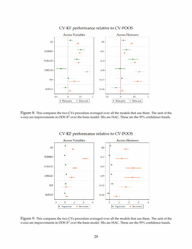
Figure 8: This compares the two CVs procedure averaged over all the models that use them. The unit of thex-axis are improvements in OOS R2 over the basis model. SEs are HAC. These are the 95% confidence bands.

Figure 9: This compares the two CVs procedure averaged over all the models that use them. The unit of thex-axis are improvements in OOS R2 over the basis model. SEs are HAC. These are the 95% confidence bands.

29

can be quite harmful. K-fold, by taking the average over the whole sample, is less immuneto such problems. Since results in 5.1 point in the direction that smaller models are betterin expansions and bigger models in recessions, the behavior of CV and how it picks theeffective complexity of the model can have an important effect on overall predictive ability.This is exactly what we see in Figure 9: CV-POOS is having a hard time in recessions withrespect to K-fold.13

5.2.4 Loss Function

In this section, we investigate whether replacing the l2 norm as an in-sample loss functionfor the SVR machinery helps in forecasting. We again use as baseline models ARs and ARDIstrained by the same corresponding CVs. The very nature of this ML feature is that the modelis less sensible to extreme residuals, thanks to the ε-insensitivity tube. We first comparelinear models in Figure 10. Clearly, changing the loss function is mostly very harmful andthat is mostly due to recessions period. However, in expansion, the linear SVR is better onaverage than a standard ARDI for UNRATE and SPREAD, but these small gains are clearlyoffset (on average) by the huge recession losses.

The SVR (or the better-known SVM) is usually used in its non-linear form. We herebycompare KRR and SVR-NL to study whether the loss function effect could reverse when anon-linear model is considered. Comparing these models makes sense since they both usethe same kernel trick (with a RBF kernel). Hence, like linear models of Figure 10, modelsin Figure 11 only differ by the use of a different loss function L. It turns out conclusionsare exactly the same as for linear models with the negative effects being slightly larger. Fur-thermore, Figures 18 and 19 confirm that these findings are found in both the data-rich andthe data-poor environments. Hence, these results confirms that L is not the most salient fea-ture of ML, at least for macroeconomic forecasting. If researchers are interested in using itsassociated kernel trick to bring in non-linearities, they should rather use the lesser-knownKRR.

13Of course, CV-POOS has hyper-hyperparameters of its own as described in detail in the appendix D andthese can change moderately the outcome. For instance, considering an expanding test window in the cross-validation recursive scheme could reduce greatly its volatility. However, the setup of the CV-POOS used inthis paper corresponds to what is standard in the literature.

30

Figure 10: This graph display the marginal (un)improvments by variables and horizons to opt for the SVRin-sample loss function in both the data-poor and data-rich environments. The unit of the x-axis are improve-ments in OOS R2 over the basis model. SEs are HAC. These are the 95% confidence bands.

Figure 11: This graph display the marginal (un)improvments by variables and horizons to opt for the SVRin-sample loss function in both recession and expansion periods. The unit of the x-axis are improvements inOOS R2 over the basis model. SEs are HAC. These are the 95% confidence bands.

31

6 Conclusion

In this papers we have studied important underlying features driving machine learningtechniques in the context of macroeconomic forecasting. We have considered many machinelearning methods in a substantive POOS setup over almost 40 years for 5 key variables and 5different horizons. We have classified these models by “features” of machine learning: non-linearities, regularization, cross-validation and alternative loss function. The four aspectsof ML are nonlinearities, regularization, cross-validation and alternative loss function. Thedata-rich and data-poor environments were considered. In order to recover their marginaleffects on forecasting performance, we designed a series of experiments that easily allow toidentify the treatment effects of interest.

The first result point in the direction that non-linearities are the true game-changer for thedata rich environment, especially when predicting real activity series and at long horizons.This gives a stark recommendation for practitioners. It recommends for most variables andhorizons what is in the end a partially non-linear factor model – that is, factors are stillobtained by PCA. The best of ML (at least of what considered here) can be obtained bysimply generating the data for a standard ARDI model and then feed it into a ML non-linear function of choice. The second result is that the standard factor model remains thebest regularization. Third, if cross-validation has to be applied to select models’ features,the best practice is the standard K-fold. Finally, one should stick with the standard L2 lossfunction.

References

Ahmed, N. K., Atiya, A. F., Gayar, N. E., and El-Shishiny, H. (2010). An empirical comparisonof machine learning models for time series forecasting. Econometric Reviews, 29(5):594–621.

Athey, S. (2018). The impact of machine learning on economics. The Economics of ArtificialIntelligence, NBER volume, Forthcoming.

Bai, J. and Ng, S. (2002). Determining the number of factors in approximate factor models.Econometrica, 70(1):191–221.

Bergmeir, C. and Benítez, J. M. (2012). On the use of cross-validation for time series predictorevaluation. Information Sciences, 191:192–213.

Bergmeir, C., Hyndman, R. J., and Koo, B. (2018). A note on the validity of cross-validationfor evaluating autoregressive time series prediction. Computational Statistics and Data Anal-ysis, 120:70–83.

Boh, S., Borgioli, S., Coman, A. B., Chiriacescu, B., Koban, A., Veiga, J., Kusmierczyk, P.,

32

Pirovano, M., and Schepens, T. (2017). European macroprudential database. Technicalreport, IFC Bulletins chapters, 46.

Chen, J., Dunn, A., Hood, K., Driessen, A., and Batch, A. (2019). Off to the races: A compari-son of machine learning and alternative data for predicting economic indicators. Technicalreport, Bureau of Economic Analysis.

Claeskens, G. and Hjort, N. L. (2008). Model selection and model averaging. Cambridge Uni-versity Press, Cambridge, U.K.

De Mol, C., Giannone, D., and Reichlin, L. (2008). Forecasting using a large number ofpredictors: Is bayesian shrinkage a valid alternative to principal components? Journal ofEconometrics, 146:318–328.

Diebold, F. X. and Mariano, R. S. (1995). Comparing predictive accuracy. Journal of Businessand Economic Statistics, 13:253–263.

Diebold, F. X. and Shin, M. (2018). Machine learning for regularized survey forecast com-bination: Partially-egalitarian lasso and its derivatives. International Journal of Forecasting,forthcoming.

Döpke, J., Fritsche, U., and Pierdzioch, C. (2015). Predicting recessions with boosted regres-sion trees. Technical report, George Washington University, Working Papers No 2015-004,Germany.

Estrella, A. and Mishkin, F. (1998). Predicting us recessions: Financial variables as leadingindicators. Review of Economics and Statistics, 80:45–61.

Fortin-Gagnon, O., Leroux, M., Stevanovic, D., and Surprenant, S. (2018). A large cana-dian database for macroeconomic analysis. Technical report, Department of Economics,UQAM.

Giannone, D., Lenza, M., and Primiceri, G. (2015). Prior selection for vector autoregressions.Review of Economics and Statistics, 97(2):436–451.

Giannone, D., Lenza, M., and Primiceri, G. (2017). Macroeconomic prediction with big data:the illusion of sparsity. Technical report, Federal Reserve Bank of New York.

Goulet Coulombe, P. (2019). Sparse and dense time-varying parameters using machinelearning. Technical report.

Granger, C. W. J. and Jeon, Y. (2004). Thick modeling. Economic Modelling, 21:323–343.

Hansen, P., Lunde, A., and Nason, J. (2011). The model confidence set. Econometrica,79(2):453–497.

Hansen, P. R. and Timmermann, A. (2015). Equivalence between out-of-sample forecastcomparisons and wald statistics. Econometrica, 83(6):2485–2505.

33

Hastie, T., Tibshirani, R., and Friedman, J. (2017). The Elements of Statistical Learning. SpringerSeries in Statistics. Springer-Verlag, New York.

Kilian, L. and Lütkepohl, H. (2017). Structural vector autoregressive analysis. Cambridge Uni-versity Press.

Kotchoni, R., Leroux, M., and Stevanovic, D. (2017). Macroeconomic forecast accuracy in adata-rich environment. Technical report, CIRANO, 2017s-05.

Litterman, R. B. (1979). Techniques of forecasting using vector autoregressions. Technicalreport.

Marcellino, M., Stock, J. H., and Watson, M. W. (2006). A comparison of direct and iteratedmultistep ar methods for forecasting macroeconomic time series. Journal of Econometrics,135:499–526.

McCracken, M. W. and Ng, S. (2016). Fred-md: A monthly database for macroeconomicresearch. Journal of Business and Economic Statistics, 34(4):574–589.

Mullainathan, S. and Spiess, J. (2017). Machine learning: An applied econometric approach.Journal of Economic Perspectives, 31(2):574–589.

Nakamura, E. (2005). Inflation forecasting using a neural network. Economics Letters,86(3):373–378.

Ng, S. (2014). Boosting recessions. Canadian Journal of Economics, 47(1):1–34.

Sermpinis, G., Stasinakis, C., Theolatos, K., and Karathanasopoulos, A. (2014). Inflation andunemployment forecasting with genetic support vector regression. Journal of Forecasting,33(6):471–487.

Smalter, H. A. and Cook, T. R. A. (2017). Macroeconomic indicator forecasting with deepneural networks. Technical report, Federal Reserve Bank of Kansas City.

Smeekes, S. and Wijler, E. (2018). Macroeconomic forecasting using penalized regressionmethods. International Journal of Forecasting, 34(3):408–430.

Smola, A. J. and Schölkopf, B. (2004). A tutorial on support vector regression. Statistics andcomputing, 14(3):199–211.

Stock, J. H. and Watson, M. W. (2002a). Forecasting using principal components from a largenumber of predictors. Journal of the American Statistical Association, 97:1167–1179.

Stock, J. H. and Watson, M. W. (2002b). Macroeconomic forecasting using diffusion indexes.Journal of Business and Economic Statistics, 20(2):147–162.

Tashman, L. J. (2000). Out-of-sample tests of forecasting accuracy: an analysis and review.International Journal of Forecasting, 16(4):437–450.

34

Ulke, V., Sahin, A., and Subasi, A. (2016). A comparison of time series and machine learningmodels for inflation forecasting: empirical evidence from the USA. Neural Computing andApplications, 1.

Zou, H., Hastie, T., and Tibshirani, R. (2007). On the “degrees of freedom" of the Lasso. TheAnnals of Statistics, 35(5):2173–2192.

35

A Detailed overall predictive performance

Table 3: Industrial Production: Relative Root MSPE

Full Out-of-Sample NBER Recessions PeriodsModels h=1 h=3 h=9 h=12 h=24 h=1 h=3 h=9 h=12 h=24Data-poor (H−t ) modelsAR,BIC 1 1.000 1 1.000 1 1 1 1 1 1AR,AIC 0.991* 1.000 0,999 1.000 1 0.987* 1 1 1 1AR,POOS-CV 0,998 1.044** 0,988 0.998 1.030* 1.012* 1.086*** 0.989* 1,001 1.076**AR,K-fold 0.991* 1.000 0,998 1.000 1.034* 0.987* 1 1 1 1.077**RRAR,POOS-CV 1,043 1.112* 1.028* 1.026** 0.973** 1.176** 1.229** 1.040* 1,005 0.950***RRAR,K-fold 0.985* 1.019** 0,998 1.005* 1.033** 1,022 1.049*** 1.009** 1.006** 1.061**RFAR,POOS-CV 0,999 1.031 0.977 0.951 0,992 1,023 1,043 0.914** 0.883** 1,002RFAR,K-fold 1,004 1.020 0.939* 0.933** 0.988 1,031 1,012 0.871*** 0.892*** 0.962**KRR-AR,POOS-CV 1,032 1.017 0.901* 0,995 0.949 1.122* 1,019 0.791*** 0.890*** 0.887***KRR,AR,K-fold 1,017 1.056 0.903* 0.959 0.934* 1.147* 1,136 0.799*** 0.861*** 0.887**SVR-AR,Lin,POOS-CV 0,993 1.046*** 1.043** 1.062*** 0.970** 1.026* 1.094*** 1.066*** 1.067*** 0.943***SVR-AR,Lin,K-fold 0.977** 1.017 1.050** 1.068*** 0.976** 1,001 1.047** 1.068*** 1.074*** 0.964***SVR-AR,RBF,POOS-CV 1,055 1.134** 1,042 1.042* 0,987 1.162** 1.224** 0.945** 0.955** 0.937***SVR-AR,RBF,K-fold 1,053 1.145** 1,004 0.971 0.945*** 1.253*** 1.308*** 0.913*** 0.911*** 0.949**Data-rich (H+

t ) modelsARDI,BIC 0.946* 0.991 1,037 1,004 0.968 0.801*** 0.807*** 0.887** 0.833*** 0.784***ARDI,AIC 0.959* 0.968 1,017 0.998 0.943 0.840*** 0.803*** 0.844** 0.798** 0.768***ARDI,POOS-CV 0.934** 1.042 0,999 1.020 0.925 0.807*** 0.704*** 0.767*** 0.829** 0.706***ARDI,K-fold 0.940* 0.977 1,013 0.982 0.941 0.787*** 0.812*** 0.841** 0.808** 0.730***RRARDI,POOS-CV 0.966* 1.087 0,984 0.947 0.882** 0.925** 0.900* 0.878*** 0.761*** 0.728***RRARDI,K-fold 0.934*** 0.940 0.931 0.911 0.919* 0.863*** 0.766*** 0.816*** 0.760*** 0.718***RFARDI,POOS-CV 0.957** 1.034 0.951 0.940 0.903** 0.874*** 0.847** 0.845*** 0.799*** 0.834***RFARDI,K-fold 0.961** 1.024 0.944 0.928* 0.901** 0.902*** 0.841** 0.844*** 0.813*** 0.758***KRR-ARDI,POOS-CV 1,005 1.067 0,959 0.912** 0,974 1,099 1,126 0.858*** 0.810*** 0.912*KRR,ARDI,K-fold 0.973 0.988 0.910* 0.929* 0.945 1,017 0,97 0.823*** 0.858*** 0.808***(B1, α = α),POOS-CV 0,993 1.122* 1,072 0.969 0.940 1,066 1,152 0,99 0.890** 0.873**(B1, α = α),K-fold 0.921*** 0.972 0,973 0.961 0,991 0.871*** 0.847*** 0.922* 0.822*** 0.778***(B1, α = 1),POOS-CV 0,997 1.108* 1.071* 1.003 0.929* 1,055 1,165 1 0,949 0.828***(B1, α = 1),K-fold 0.961** 1.024 1,039 1,015 0.975 0,964 0,946 0,964 0.911** 0.802***(B1, α = 0),POOS-CV 1,003 0.963 0.969 0.996 0,982 1,067 0.791*** 0.851*** 0,962 0,916(B1, α = 0),K-fold 0.934*** 0.918** 0.938 0.930 0.932 0.871*** 0.793*** 0.838*** 0.788*** 0.771***(B2, α = α),POOS-CV 1,041 1.099 1.078* 1,061 0,985 1.189** 1.177* 1,015 0,963 0.923*(B2, α = α),K-fold 0.963** 0.975 0,971 0.992 0,97 0,994 0.932* 0.928** 0.876*** 0.821***(B2, α = 1),POOS-CV 1,026 1.096 1,075 1.103* 0.922** 1.136* 1,157 1,005 0,991 0.897**(B2, α = 1),K-fold 0.943*** 0.916** 0.948 0.954 0,975 0.899*** 0.811*** 0.875*** 0.825*** 0.830***(B2, α = 0),POOS-CV 1,013 1.099** 1.102* 1.107* 0.969 1.091* 1.116* 1,026 0,942 0.870**(B2, α = 0),K-fold 0,981 1.010 1,017 1,029 1 0,971 1,008 0,943 0.871** 0.825***(B3, α = α),POOS-CV 1,038 1.106* 1,042 1.002 0.933* 1.128** 1,16 1,014 0.928* 0.852***(B3, α = α),K-fold 0.945*** 1.003 1,082 1,038 0.932 0.922** 0,977 0.878** 0.823*** 0.784***(B3, α = 1),POOS-CV 1.077* 1.121* 1,034 1,033 0,974 1.175** 1,131 0,996 0.917** 0.901**(B3, α = 1),K-fold 0.950** 0.978 1,074 1.088* 1,031 0.929** 0.883** 0.841*** 0.846** 0.833**(B3, α = 0),POOS-CV 1,037 1.183*** 1.148** 1.127* 1,008 1.166** 1.246** 1.129* 1,028 0.862***(B3, α = 0),K-fold 1.305** 1.517** 1.079** 1,008 1.110*** 1,238 1.438** 1,003 0,96 1SVR-ARDI,Lin,POOS-CV 0.945** 1.008 1,081 0.967 0.948 0.907* 0.815*** 0.869** 0.799*** 0.737***SVR-ARDI,Lin,K-fold 0.911*** 0.920* 1,015 0.987 0,984 0.821*** 0.761*** 0.866** 0.805*** 0.743***SVR-ARDI,RBF,POOS-CV 1,045 1.140** 0,995 0.979 0.962 1.158* 1.226** 0,952 0.907*** 0.894***SVR-ARDI,RBF,K-fold 1.072* 1.132*** 0.948 0.956 0.918*** 1.290*** 1.205*** 0.824*** 0.843*** 0.861***

Note: The numbers represent the relative, with respect to AR,BIC model, root MSPE. Models retained in model confidence set are in bold, the minimum

values are underlined, while ∗∗∗, ∗∗, ∗ stand for 1%, 5% and 10% significance of Diebold-Mariano test.

36

Table 4: Unemployment rate: Relative Root MSPE

Full Out-of-Sample NBER Recessions PeriodsModels h=1 h=3 h=9 h=12 h=24 h=1 h=3 h=9 h=12 h=24Data-poor (H−t ) modelsAR,BIC 1 1 1 1 1 1 1 1 1 1AR,AIC 0,991 0,984 0,988 0.993*** 1 0,958 0.960** 0.984* 1 1AR,POOS-CV 0,989 1.042* 0,996 0,996 0,98 0,977 1.103* 0.981** 0,998 1,024AR,K-fold 0,987 0,984 0.990* 0.994*** 0.974** 0.982* 0.960** 1 1,001 1RRAR,POOS-CV 1,005 1.050* 1,008 0,99 0.979* 1.083** 1.151** 1,006 1,006 0,997RRAR,K-fold 0.984* 0.982* 0,994 0,996 0,993 0,983 0,984 0,992 1,001 1,029RFAR,POOS-CV 0,999 1,011 0,987 1,002 1 1.107** 1,046 0.921** 0,962 0,997RFAR,K-fold 0,982 0,986 0,977 0,987 1,003 0,966 0,971 0.911*** 0.947** 0.946**KRR-AR,POOS-CV 0.982 1,012 0.892** 0.837*** 0.821*** 1,093 1,151 0.858*** 0.747*** 0.841***KRR,AR,K-fold 0.925*** 0.862*** 0.842*** 0.828*** 0.803*** 0.828*** 0.804*** 0.772*** 0.736*** 0.846***SVR-AR,Lin,POOS-CV 1,037 1,068 1 0,987 0,97 1.237** 1.231*** 1.064*** 1.093*** 1.165***SVR-AR,Lin,K-fold 0,985 0.975* 0,992 0,991 0,991 0,988 1,008 1.064*** 1.092*** 1.205***SVR-AR,RBF,POOS-CV 1.044* 1.087** 1.088*** 1.036* 1.048*** 1.208** 1.177** 1.120*** 1.082*** 1.119***SVR-AR,RBF,K-fold 1.034** 1.114** 1.064** 1.052** 1,011 1.136*** 1.248*** 1.065*** 1.074*** 1.075***Data-rich (H+

t ) modelsARDI,BIC 0.937** 0.893** 0,938 0,939 0.875*** 0.690*** 0.715*** 0.798*** 0.782*** 0.783***ARDI,AIC 0.933** 0.878*** 0,928 0,953 0.893** 0.720*** 0.719*** 0.798*** 0.799*** 0.787***ARDI,POOS-CV 0.930*** 0.918* 0,931 0,937 0.869*** 0.731*** 0.675*** 0.821** 0.785*** 0.768***ARDI,K-fold 0.947* 0.893** 0,97 0,964 0.928* 0.677*** 0.665*** 0.805*** 0.807*** 0.772***RRARDI,POOS-CV 0.918*** 0,937 0,97 0,955 0.861*** 0.709*** 0.756*** 0.890** 0.832*** 0.754***RRARDI,K-fold 0.940** 0.876** 0.901* 0.911* 0.897** 0.744*** 0.676*** 0.788*** 0.819*** 0.745***RFARDI,POOS-CV 0.925*** 0.919** 0.870*** 0.879** 0.782*** 0.708*** 0.739*** 0.715*** 0.736*** 0.785***RFARDI,K-fold 0.947** 0.902*** 0.857*** 0.846*** 0.776*** 0.763*** 0.751*** 0.761*** 0.725*** 0.696***KRR-ARDI,POOS-CV 0,993 0.990 0.883** 0.835*** 0.779*** 1,066 1,092 0.800*** 0.734*** 0.766***KRR,ARDI,K-fold 0.940*** 0.882*** 0.841*** 0.810*** 0.802*** 0,938 0.889* 0.791*** 0.739*** 0.841***(B1, α = α),POOS-CV 0.910*** 0.936** 0,945 0,975 0.929** 0.771** 0.834** 0.879** 0.841*** 0.853***(B1, α = α),K-fold 0.920*** 0.871*** 0.913* 0,933 0,967 0.813* 0.738*** 0.839*** 0.736*** 0.712***(B1, α = 1),POOS-CV 0.928*** 0,975 1.092* 1,041 0.906*** 0.861** 0.886** 0,986 0.906* 0.837***(B1, α = 1),K-fold 0.912*** 0.888*** 0,994 0,984 0.924** 0.798*** 0.745*** 0,906 0.834*** 0.766***(B1, α = 0),POOS-CV 0.922*** 0,947 0,982 0,961 0.934* 0.802** 0.809*** 0.893* 0,897 0.843**(B1, α = 0),K-fold 0.921*** 0.876*** 0.893** 0.911** 0.929* 0.824** 0.788** 0.820*** 0.771*** 0.731***(B2, α = α),POOS-CV 0.950** 0.922** 0,971 1,002 0.856*** 0,898 0.856** 0.902* 0.857*** 0.831***(B2, α = α),K-fold 0.930*** 0.867*** 0.898** 0.917** 0.892*** 0.827*** 0.773*** 0.869*** 0.831*** 0.750***(B2, α = 1),POOS-CV 0.944*** 0.900*** 0,952 0,996 0.892*** 0.787*** 0.770*** 0.889** 0.869** 0,978(B2, α = 1),K-fold 0.937*** 0.914*** 0.849*** 0.915** 0.872*** 0.736*** 0.791*** 0.837*** 0.873** 0.842***(B2, α = 0),POOS-CV 0.979 1,001 1,031 1,011 0.946* 1,085 1,061 0,947 0.826*** 0.835**(B2, α = 0),K-fold 0.957** 0.939** 0,988 1,004 0,951 0,991 1,006 0,97 0.875** 0.763***(B3, α = α),POOS-CV 0,975 0,974 0,984 0.922* 0.882*** 0,999 0,969 0.916** 0.893** 0.834**(B3, α = α),K-fold 0.955*** 0.872*** 0,945 0,94 0.897** 0.882*** 0.772*** 0.840*** 0.835*** 0.829**(B3, α = 1),POOS-CV 0.912*** 0,953 0,981 0,949 0.910** 0.793** 0.843*** 0.895** 0.923* 0,919(B3, α = 1),K-fold 0.937*** 0.923*** 0,954 0,939 0.917* 0.811*** 0.821*** 0.852*** 0.823*** 0.838**(B3, α = 0),POOS-CV 1.197** 1.144*** 1.318** 1.233** 1 1.470** 1.269*** 1.288** 1,123 0.787***(B3, α = 0),K-fold 1.219* 1,039 1.108** 1.236** 1.082* 1,417 1,077 1,095 1,232 0,971SVR-ARDI,Lin,POOS-CV 0.919*** 0.921* 0.906* 0,947 0.911** 0.748*** 0.734*** 0.861** 0.794*** 0.835***SVR-ARDI,Lin,K-fold 0.939*** 0.864*** 0.877** 0.858*** 0.888*** 0.777*** 0.726*** 0.777*** 0.750*** 0.791***SVR-ARDI,RBF,POOS-CV 1,035 1.133** 1,018 0.945** 0.926*** 1.182** 1.278*** 1,017 0.885*** 0.931*SVR-ARDI,RBF,K-fold 1,032 1,032 0,954 0.921** 0.870*** 1,102 1,058 0.894*** 0.864*** 0.874**

Note: The numbers represent the relative, with respect to AR,BIC model, root MSPE. Models retained in model confidence set are in bold, the minimum

values are underlined, while ∗∗∗, ∗∗, ∗ stand for 1%, 5% and 10% significance of Diebold-Mariano test.

37

Table 5: Term spread: Relative Root MSPE

Full Out-of-Sample NBER Recessions PeriodsModels h=1 h=3 h=9 h=12 h=24 h=1 h=3 h=9 h=12 h=24Data-poor (H−t ) modelsAR,BIC 1 1.000 1.000 1.000 1.000 1 1 1 1 1AR,AIC 1.002* 0.998 1.053* 1.034** 1.041** 1,002 1,001 1,034 0,993 0.972AR,POOS-CV 1,002 1.140* 1.005 0.988 1.035* 1 1,017 0.873** 0.872** 0.973AR,K-fold 1.054* 1.065* 0.998 1.000 1.034* 1,041 1 0,907 1 0,983RRAR,POOS-CV 1.012** 1.145* 1.011 1.016* 1,016 1,011 1,015 0.966** 0.987* 0.930**RRAR,K-fold 1.046* 0.997 1,043 0.972 1,021 1,025 0,997 0,995 0.820** 0.954*RFAR,POOS-CV 1,006 0.899 1.110** 0,996 1.086** 0,908 0,839 1,042 0.713** 1.048*RFAR,K-fold 0,986 0.929 1.124*** 1,014 1.083** 0.892 0,793 1,006 0.754* 1.053*KRR-AR,POOS-CV 1.203* 0.876 0.978 0.868** 0.887*** 0.894 0.703* 0.776*** 0.658** 0.945KRR,AR,K-fold 1.203* 0.867* 0.936* 0.871** 0.894*** 0.879 0,708 0.791*** 0.665** 0.954SVR-AR,Lin,POOS-CV 0,999 0.973 0.995 1,025 0.964* 0,975 0,806 0,989 0.922* 0.998SVR-AR,Lin,K-fold 0,995 0.916 0.990 0.984 0.955** 0.966 0,706 0,998 0,972 0.949**SVR-AR,RBF,POOS-CV 1,019 0.853* 1,055 0.928 0.953 0.786 0,739 0,888 0.688** 0.885***SVR-AR,RBF,K-fold 1.005 0.879 1.161*** 0,998 1,052 0.786 0.668 0,957 0.732* 0.990Data-rich (H+

t ) modelsARDI,BIC 0.953 0,971 0.979 0.930 0.892*** 0,921 0,9 0.790*** 0.633*** 1,049ARDI,AIC 0.970 0.956 1.019 0.944 0.917** 0.929 0,867 0.814*** 0.647*** 1,076ARDI,POOS-CV 0.934 1,039 1,063 1,036 1.000 0.900 0,939 0,973 0,868 1,105ARDI,K-fold 0.963 0.936 0.980 0.934 0.955 0.892 0,897 0.788*** 0.647*** 1,114RRARDI,POOS-CV 0,972 1,022 1.095* 1,003 1,025 0,948 0,925 0,998 0.827* 1.183*RRARDI,K-fold 0,97 0,99 0.983 0.955 0.962 0,934 0,967 0.777*** 0.682** 1,102RFARDI,POOS-CV 1,002 0.832* 0.956 0.856** 0.919** 0.817 0.684 0.790*** 0.626*** 0.965RFARDI,K-fold 1,061 0.872* 1,014 0.887* 0.950 0.863 0,736 0.856* 0.652** 0.961KRR-ARDI,POOS-CV 1.311*** 0.908 1.018 0.852** 0.907*** 0.904 0.663* 0.716*** 0.603*** 0.931KRR,ARDI,K-fold 1.376** 0.947 0.968 0.846** 0.877*** 0.862 0.686 0.766*** 0.575*** 0.930*(B1, α = α),POOS-CV 1,043 0,988 1.164*** 1.085* 0.924** 0,979 0,907 1,075 0,951 1,026(B1, α = α),K-fold 0,995 0,981 1.087* 1,028 0.939 0,94 0,929 0,91 0.789** 1,003(B1, α = 1),POOS-CV 1,068 0.954 1.185** 1,074 0.991 0.915 0,86 1.399* 0.807* 1.104**(B1, α = 1),K-fold 1,041 0.937 0.961 0.982 0.943** 0,937 0,854 0.789*** 0.664** 1,01(B1, α = 0),POOS-CV 1.426** 1.138* 1.215*** 1,052 0.967 1.473* 1,018 1.283* 0.808* 1,07(B1, α = 0),K-fold 1.359* 1,041 1,038 0.980 0.905** 1,404 1,044 0.869* 0.737** 0.978(B2, α = α),POOS-CV 0,987 0,979 1.149*** 1,01 1,008 0.879 0,874 0,97 0.731** 1,09(B2, α = α),K-fold 0,979 0.959 1.006 0.965 0.937** 0.872 0,885 0.819** 0.666** 0.912**(B2, α = 1),POOS-CV 1.121* 1,086 1.008 1 0.965 1,002 1,078 0.840*** 0.766** 0.955(B2, α = 1),K-fold 1,006 0.916 0.983 0.918 0.901*** 0.880 0,815 0.811*** 0.648** 1,024(B2, α = 0),POOS-CV 1.136** 1,018 1.150*** 1,045 1.010 0,971 0,908 1,086 0,838 0.958(B2, α = 0),K-fold 1.146** 0.952 1,042 0.961 0.954 0,946 0,879 0.887* 0.789* 0.900**(B3, α = α),POOS-CV 1.183* 1.145** 1.157*** 1,034 0.949 0,923 1,012 0.826*** 0.623*** 0,993(B3, α = α),K-fold 1.176* 1,074 1.167*** 1,048 0.929* 0,956 1,023 0.812** 0.754** 0.975(B3, α = 1),POOS-CV 1.305*** 1.302*** 1.140*** 0,981 0.948 1,042 1,071 0.855** 0.656*** 1,009(B3, α = 1),K-fold 1.222* 1,086 1.093** 1,039 0.972 1,004 0,889 0,913 0.736** 0.976(B3, α = 0),POOS-CV 1.775*** 1.335*** 1.208*** 1.362* 0.990 1.379** 0,977 1,093 1,244 0,968(B3, α = 0),K-fold 1.644*** 1.189** 1.153*** 1,019 0.997 1.565*** 0,795 0,907 0.737** 0.980SVR-ARDI,Lin,POOS-CV 0.927 0.988 1.024 0.941 0.962 0.888 0,953 0.856** 0.729** 1.114*SVR-ARDI,Lin,K-fold 0.975 0.924 1.007 0.928 0.899*** 0.944 0,851 0.842*** 0.681** 1,03SVR-ARDI,RBF,POOS-CV 1.733*** 1,031 1,061 0.935 0.900*** 1.377** 0,799 0.761*** 0.651** 0.931SVR-ARDI,RBF,K-fold 1.692*** 1.002 1,034 0.933 0.948* 1.377** 0,802 0.795** 0.648** 0.976

Note: The numbers represent the relative, with respect to AR,BIC model, root MSPE. Models retained in model confidence set are in bold, the minimum

values are underlined, while ∗∗∗, ∗∗, ∗ stand for 1%, 5% and 10% significance of Diebold-Mariano test.

38

Table 6: CPI Inflation: Relative Root MSPE

Full Out-of-Sample NBER Recessions PeriodsModels h=1 h=3 h=9 h=12 h=24 h=1 h=3 h=9 h=12 h=24Data-poor (H−t ) modelsAR,BIC 1.000 1.000 1.000 1 1 1 1.000 1 1 1AR,AIC 0.965*** 1.000 1.000 0.969** 0.968** 0,998 0.998 1 0,998 0,972AR,POOS-CV 0.977 0.997 0.977 0.957** 0.943*** 0,978 0.992 1 0,979 0,977AR,K-fold 0.966*** 0.986 0.974* 0.967** 0.970** 0,998 0.975** 1 1,007 0,992RRAR,POOS-CV 0.962*** 1.003 0.978 0.976 0.946*** 0.963** 0.990 0,998 0,977 0,971RRAR,K-fold 1.020* 1.015 1.182* 0.981 0,986 0,999 1.008 1,077 0,999 1.002*RFAR,POOS-CV 1.012 1.165** 1.285*** 1.279*** 1.274*** 0,931 1,147 1,08 1.089** 1.256***RFAR,K-fold 1,021 1.188*** 1.269*** 1.285*** 1.310*** 0,959 1.159* 1,042 1.125** 1.266**KRR-AR,POOS-CV 0.993 1.144** 1.288*** 1.330** 1.263** 0.884* 1,143 0,944 1,053 1.279**KRR,AR,K-fold 1.004 1.116* 1.226** 1.234** 1,163 0.893* 1,14 0,911 0,952 0,93SVR-AR,Lin,POOS-CV 1.010 1.191*** 1.376*** 1.365*** 1.337*** 0.902* 1,13 1.148* 1.146** 1.222**SVR-AR,Lin,K-fold 1.003 1.201*** 1.354*** 1.355*** 1.321*** 0.901* 1.139* 1.123* 1.149** 1.220**SVR-AR,RBF,POOS-CV 1.053* 1.260*** 1.539*** 1.515*** 1.471*** 0,905 1.191* 1,122 1.166** 1.337***SVR-AR,RBF,K-fold 1,039 1.253*** 1.462*** 1.488*** 1.416*** 0,906 1.185* 1.119* 1.222** 1.263*Data-rich (H+

t ) modelsARDI,BIC 0.958 1.005 1.022 1.006 1,004 0,928 0.938 0.745** 0.688** 0.568**ARDI,AIC 0.975 1.014 1.033 1,04 1,033 0,958 0.923 0.740** 0.661** 0.474**ARDI,POOS-CV 0.979 1.113 1.005 1,041 1,014 0,963 1,041 0.789** 0.711*** 0.530**ARDI,K-fold 0.945 1.015 1.008 1,045 1,009 0,906 0.927 0.753** 0.662** 0.456**RRARDI,POOS-CV 0.975 1.099 0.984 1,075 1,058 0,937 1,034 0.789** 0.688*** 0.504**RRARDI,K-fold 0.943* 1.012 1.046 0.935 1,044 0.894** 0.913 0.767* 0.658*** 0.465**RFARDI,POOS-CV 1.025 1.165** 1.254*** 1.261*** 1.179** 0,936 1,143 0,982 0,948 0,985RFARDI,K-fold 1.024 1.178** 1.267*** 1.274*** 1.214** 0,955 1,176 0,976 0,95 1,014KRR-ARDI,POOS-CV 0.978 1.149** 1.300*** 1.233** 1.161* 0.902* 1,131 0,996 0,968 0,917KRR,ARDI,K-fold 1.004 1.137** 1.271*** 1.244** 1,157 0.904* 1,117 0,984 0.882* 0,954(B1, α = α),POOS-CV 0.954* 1.062* 1.112** 1.087* 1,086 0.873* 1,053 0,924 0.824** 0,804(B1, α = α),K-fold 0.937** 1.047 1.136** 1,062 1,125 0.863* 1,074 0,986 0.877* 0,812(B1, α = 1),POOS-CV 0.977 1.136* 1.185*** 1.096* 1.217** 0.880* 1,213 1,04 0,921 0,873(B1, α = 1),K-fold 0.978 1.138* 1.154** 1.091* 1,093 0,915 1,222 1,075 0,96 0.592*(B1, α = 0),POOS-CV 0.977 1.052 1.612* 1.250*** 1.266** 0.904 1.005 2,139 1,067 0,786(B1, α = 0),K-fold 0.948 1,315 1.109** 1.359** 1,412 0.839* 1,57 0,961 1,355 0,76(B2, α = α),POOS-CV 0.970 1.051* 1.089* 1.104* 1.122* 0.891* 1,027 0,885 0,89 0,844(B2, α = α),K-fold 0.977 1.039 1.086* 1,079 1.112* 0,904 1,033 0,891 0,901 0,871(B2, α = 1),POOS-CV 0.997 1.075** 1.106* 1.115* 1.151* 0,913 1,066 0,902 0,923 0,888(B2, α = 1),K-fold 0.973 1.053* 1.137** 1,099 1.191** 0,919 1,022 0,886 0,921 0,958(B2, α = 0),POOS-CV 1.001 1.104** 1.136*** 1.186*** 1.327*** 0,935 1,093 0,988 1,071 0,889(B2, α = 0),K-fold 0.993 1.085** 1.144*** 1.132** 1.216*** 0,923 1,076 0,965 1,045 0,896(B3, α = α),POOS-CV 0.973 1.128*** 1.211*** 1.274** 1.225*** 0.819** 1,09 1,023 1.095* 0,918(B3, α = α),K-fold 0.976 1.098*** 1.231*** 1.211*** 1.125** 0.837** 1,061 1,108 1,013 0,864(B3, α = 1),POOS-CV 0.999 1.117*** 1.219*** 1.313*** 1.232*** 0.830** 1,076 1,08 0,976 0,876(B3, α = 1),K-fold 0.990 1.134*** 1.260*** 1.241*** 1.176*** 0.853* 1,054 1.132* 1,069 0,862(B3, α = 0),POOS-CV 1.085 1.400** 1.330*** 1.468*** 1.267*** 0.900 1,056 1.173** 1.490** 0,831(B3, α = 0),K-fold 0.976 1.276** 1.328*** 1.392*** 1.244*** 0.864* 1,064 1.348** 1.439*** 0,858SVR-ARDI,Lin,POOS-CV 1,019 1.134** 1.200*** 1.326** 1.189* 0,969 1,055 1 0,974 0,735SVR-ARDI,Lin,K-fold 0.964 1.108** 1.191** 1.200** 1,167 0.865** 1,084 1,018 0.769** 0,689SVR-ARDI,RBF,POOS-CV 1,04 1.263*** 1.534*** 1.515*** 1.461*** 0,906 1,153 1.119* 1.195** 1.243*SVR-ARDI,RBF,K-fold 1,037 1.253*** 1.522*** 1.500*** 1.433*** 0,907 1,155 1.124* 1.187* 1.252*

Note: The numbers represent the relative, with respect to AR,BIC model, root MSPE. Models retained in model confidence set are in bold, the minimum

values are underlined, while ∗∗∗, ∗∗, ∗ stand for 1%, 5% and 10% significance of Diebold-Mariano test.

39

Table 7: Housing starts: Relative Root MSPE

Full Out-of-Sample NBER Recessions PeriodsModels h=1 h=3 h=9 h=12 h=24 h=1 h=3 h=9 h=12 h=24Data-poor (H−t ) modelsAR,BIC 1 1.000 1.000 1.000 1.000 1 1.000 1 1 1AR,AIC 0.995 0.987 1.048* 1.008 1.041* 0.956*** 0.976* 1,007 0,97 0.955AR,POOS-CV 1.010* 1.002 1.064** 1.011 1.049*** 0.989* 1.011* 1.025** 0,991 0,981AR,K-fold 0.992 0.986 1.029 0.997 1.031 0.957*** 0.973** 0,999 0,954 0.925**RRAR,POOS-CV 1.028** 1.022 0.983 0.905* 0.954 0,987 1.018 0.943 0.912* 1,05RRAR,K-fold 0.990 0.986* 1.035 0.992 1.024 0.935*** 0.974** 1,013 0,965 0.924**RFAR,POOS-CV 1.231** 1.267** 1.260** 1.271** 1.086** 1.463* 1.588** 1,058 1,01 0.941*RFAR,K-fold 1.179* 1.255** 1.314** 1.264** 1.058* 1.452* 1.586** 1.073* 0,973 0.883**KRR-AR,POOS-CV 2.008*** 1.811*** 1.567*** 1.384*** 0.980** 2.141*** 1.927*** 1.088* 0,944 0.981*KRR,AR,K-fold 1.293** 1.325* 1.430** 1.165** 1.001 1.684** 1.778** 1.107** 0,937 0.974**SVR-AR,Lin,POOS-CV 1.220** 1.411** 1.307** 1.284*** 1.040 1.286* 1.600* 1.056* 1.108** 1.114*SVR-AR,Lin,K-fold 1.219** 1.501** 1.313*** 1.240*** 1.011 1.449* 1.573* 1,037 1,05 1,024SVR-AR,RBF,POOS-CV 1.281*** 1.315** 1.336** 1.251*** 1.014 1.517** 1.627** 1.092* 1 0,962SVR-AR,RBF,K-fold 1.155*** 1.443*** 1.421*** 1.338*** 1.080*** 1.265** 1.624* 1.088* 1,043 1,011Data-rich (H+

t ) modelsARDI,BIC 0.951** 0.958 1.034 1.026 1.045 0.929 1.104* 0,96 0.862** 1,064ARDI,AIC 0.979 0.975 1.018 1.034 1.078** 0.958 1.151** 0.936 0.905* 1,036ARDI,POOS-CV 0,996 0.981 1.077* 1.040 1.091** 0,962 1.133* 0,968 0,915 0,987ARDI,K-fold 0.979 0.989 1.028 1.037 1.075*** 0,977 1.154** 0,953 0.885* 1,041RRARDI,POOS-CV 1,004 1.044 1.042 1.012 1.004 0.939* 1.216** 0.942* 0.907 1.096*RRARDI,K-fold 0.970 0.981 1.043 1.034 0.964 0.932 1.136** 0.915** 0.867** 1,01RFARDI,POOS-CV 1.224* 1.238* 1.174** 1.141* 1.004 1.608* 1.602** 1,019 0,926 0,969RFARDI,K-fold 1,131 1.216* 1.209** 1.128** 0.973 1.401* 1.615** 1,046 0.929* 0.940KRR-ARDI,POOS-CV 1.346*** 1.456** 1.348** 1.242** 1.002 1.562** 1.887** 1,028 0,98 0.963***KRR,ARDI,K-fold 1.466*** 1.410** 1.474** 1.300** 1.022 1.856*** 1.907** 1.106** 0,981 1(B1, α = α),POOS-CV 1.102** 1.110 1.158** 1.126** 1.032 1.197** 1.387*** 1,029 0,947 1,001(B1, α = α),K-fold 1.057* 1.050 1.135** 1.110** 1.009 1.124* 1.281*** 0,987 0.929** 0.980(B1, α = 1),POOS-CV 0.960 1.038 1.274*** 1.158*** 0.989 0.940 1.317** 1,017 0.901** 1,009(B1, α = 1),K-fold 0.950* 1.022 1.203*** 1.163** 0.981 0.945 1.285** 0,971 0.890** 1,019(B1, α = 0),POOS-CV 1.191*** 1.214** 1.136** 1.203** 1.055* 1.227* 1.594*** 0,975 0.914* 0,99(B1, α = 0),K-fold 1.091* 1.155 1.104* 1.085 1.044 1,198 1.536** 0.946 0.863** 0,982(B2, α = α),POOS-CV 1,053 1.092 1.040 1.054 1.018 1.170* 1.368*** 0,969 0,936 0.958*(B2, α = α),K-fold 1.058* 1.020 1.064 1.033 1.057** 1.183** 1.253** 0,989 0.909* 0,999(B2, α = 1),POOS-CV 1,015 1.009 1.079 1.101** 1.024 1,036 1.234** 0,962 0.904** 0.909**(B2, α = 1),K-fold 0,991 0.994 1.019 1.009 1.013 0,981 1.226** 0.931 0.841*** 1,005(B2, α = 0),POOS-CV 1.224*** 1.293** 1.202*** 1.168** 1.002 1.378** 1.639** 1,007 0.887*** 0.897**(B2, α = 0),K-fold 1.147*** 1.175 1.070 1.006 0.995 1.261*** 1.589** 0,973 0.884*** 0,955(B3, α = α),POOS-CV 1.380*** 1.283** 1.223** 1.147** 1.046 1.531*** 1.566*** 1.089* 0,978 0.943*(B3, α = α),K-fold 1.420*** 1.248*** 1.186** 1.176** 1.049 1.370*** 1.436*** 1,027 0,972 0,993(B3, α = 1),POOS-CV 1.132** 1.033 1.181** 1.145** 1.036 1.175* 1.179* 0.933* 0.906** 0.926*(B3, α = 1),K-fold 1.085** 1.061 1.169** 1.159** 1.081 1,013 1.257** 0,954 0,923 0,998(B3, α = 0),POOS-CV 1.595*** 1.468*** 1.352*** 1.204** 1.041** 1.588*** 1.622*** 0.956 0.908* 1,013(B3, α = 0),K-fold 1.505*** 1.367*** 1.375*** 1.252** 0.984 1.634*** 1.490*** 1.104* 1,037 0,952SVR-ARDI,Lin,POOS-CV 1.231*** 1.207** 1.179** 1.152** 1.134*** 1.333** 1.386*** 1,087 1,026 1,023SVR-ARDI,Lin,K-fold 1.208*** 1.442** 1.107* 1,101 1.074** 1,097 1.222** 0.925* 0.846** 1,007SVR-ARDI,RBF,POOS-CV 1.621*** 1.778*** 1.425*** 1.263** 0.985 1.745*** 1.956** 1,077 0,919 1SVR-ARDI,RBF,K-fold 1.675*** 1.802*** 1.467*** 1.267** 1.023 1.808*** 1.993** 1,079 0.924* 0,989

Note: The numbers represent the relative, with respect to AR,BIC model, root MSPE. Models retained in model confidence set are in bold, the minimum

values are underlined, while ∗∗∗, ∗∗, ∗ stand for 1%, 5% and 10% significance of Diebold-Mariano test.

40

B Robustness of Treatment Effects Graphs

Figure 12: This figure plots the distribution of α(h,v)F from equation 11 done by (h, v) subsets. The subsample

under consideration here is data-poor models. The unit of the x-axis are improvements in OOS R2 over thebasis model. Variables are INDPRO, UNRATE, SPREAD, INF and HOUST. Within a specific color block, thehorizon increases from h = 1 to h = 24 as we are going down. SEs are HAC. These are the 95% confidencebands.

41

Figure 13: This figure plots the distribution of α(h,v)F from equation 11 done by (h, v) subsets. The subsample

under consideration here is data-rich models. The unit of the x-axis are improvements in OOS R2 over thebasis model. Variables are INDPRO, UNRATE, SPREAD, INF and HOUST. Within a specific color block, thehorizon increases from h = 1 to h = 24 as we are going down. SEs are HAC. These are the 95% confidencebands.

Figure 14: This figure plots the distribution of α(h,v)F from equation 11 done by (h, v) subsets. The subsample

under consideration here are recessions. The unit of the x-axis are improvements in OOS R2 over the basismodel. Variables are INDPRO, UNRATE, SPREAD, INF and HOUST. Within a specific color block, the horizonincreases from h = 1 to h = 24 as we are going down. SEs are HAC. These are the 95% confidence bands.

42

Figure 15: This figure plots the distribution of α(h,v)F from equation 11 done by (h, v) subsets. The subsample

under consideration here are the last 20 years. The unit of the x-axis are improvements in OOS R2 over thebasis model. Variables are INDPRO, UNRATE, SPREAD, INF and HOUST. Within a specific color block, thehorizon increases from h = 1 to h = 24 as we are going down. SEs are HAC. These are the 95% confidencebands.

43

C Additional Graphs

Figure 16: This graph displays the marginal improvements of different ARDIs with respect to the baselineARDI-BIC. The unit of the x-axis are improvements in OOS R2 over the basis model. SEs are HAC. These arethe 95% confidence bands.

44

Figure 17: This graph displays the marginal improvements of different ARDIs with respect to the baselineARDI-BIC by variables and horizons. The unit of the x-axis are improvements in OOS R2 over the basis model.SEs are HAC. These are the 95% confidence bands.

Figure 18: This graph display the marginal (un)improvments by variables and horizons to opt for the SVRin-sample loss function in comparing the data-poor and data-rich environments for linear models. The unitof the x-axis are improvements in OOS R2 over the basis model. SEs are HAC. These are the 95% confidencebands.

45

Figure 19: This graph display the marginal (un)improvments by variables and horizons to opt for the SVR in-sample loss function in comparing the data-poor and data-rich environments for non-linear models. The unitof the x-axis are improvements in OOS R2 over the basis model. SEs are HAC. These are the 95% confidencebands.

46

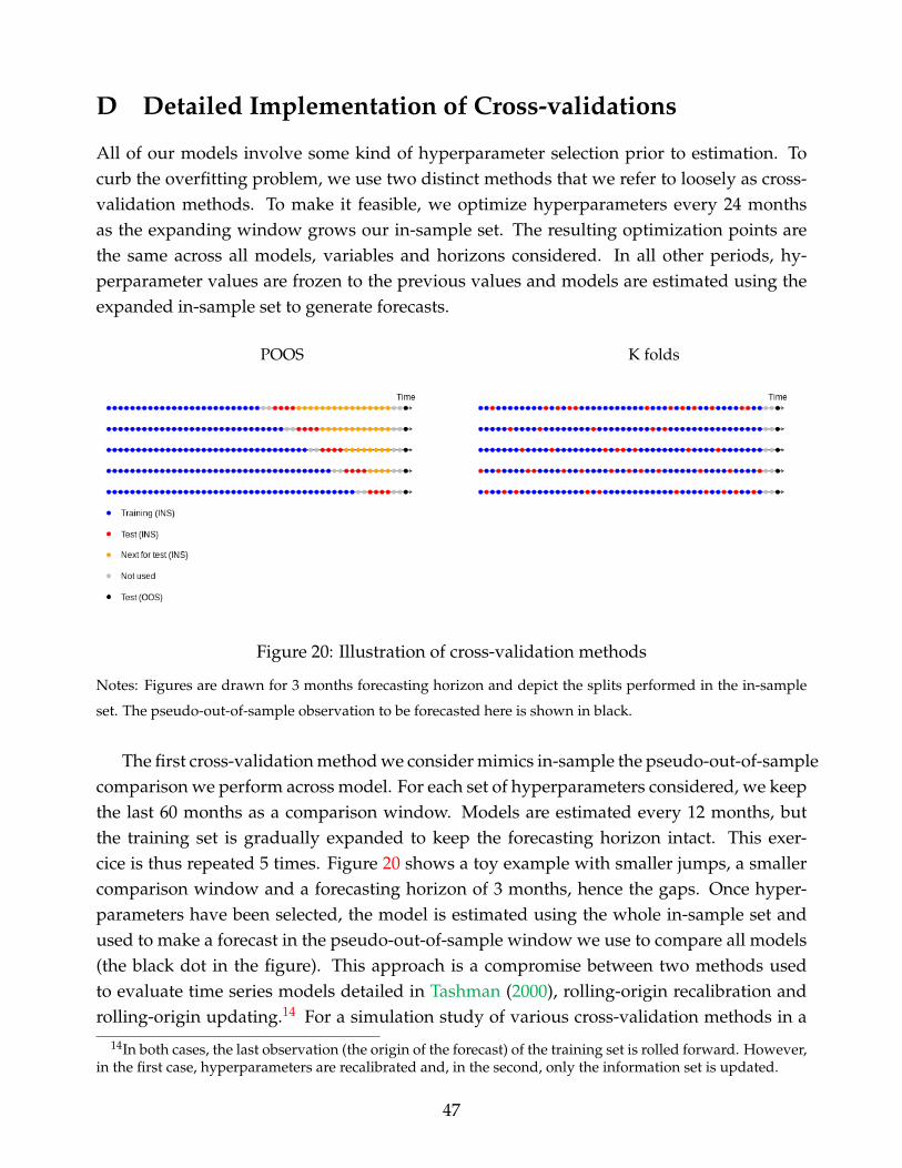
D Detailed Implementation of Cross-validations

All of our models involve some kind of hyperparameter selection prior to estimation. Tocurb the overfitting problem, we use two distinct methods that we refer to loosely as cross-validation methods. To make it feasible, we optimize hyperparameters every 24 monthsas the expanding window grows our in-sample set. The resulting optimization points arethe same across all models, variables and horizons considered. In all other periods, hy-perparameter values are frozen to the previous values and models are estimated using theexpanded in-sample set to generate forecasts.

POOS K folds

Figure 20: Illustration of cross-validation methods

Notes: Figures are drawn for 3 months forecasting horizon and depict the splits performed in the in-sample

set. The pseudo-out-of-sample observation to be forecasted here is shown in black.

The first cross-validation method we consider mimics in-sample the pseudo-out-of-samplecomparison we perform across model. For each set of hyperparameters considered, we keepthe last 60 months as a comparison window. Models are estimated every 12 months, butthe training set is gradually expanded to keep the forecasting horizon intact. This exer-cice is thus repeated 5 times. Figure 20 shows a toy example with smaller jumps, a smallercomparison window and a forecasting horizon of 3 months, hence the gaps. Once hyper-parameters have been selected, the model is estimated using the whole in-sample set andused to make a forecast in the pseudo-out-of-sample window we use to compare all models(the black dot in the figure). This approach is a compromise between two methods usedto evaluate time series models detailed in Tashman (2000), rolling-origin recalibration androlling-origin updating.14 For a simulation study of various cross-validation methods in a

14In both cases, the last observation (the origin of the forecast) of the training set is rolled forward. However,in the first case, hyperparameters are recalibrated and, in the second, only the information set is updated.

47

time series context, including the rolling-origin recalibration method, the reader is referredto Bergmeir and Benítez (2012). We stress again that the compromise is made to bring downcomputation time.

The second cross-validation method, K-fold cross-validation, is based on a re-samplingscheme (Bergmeir et al. (2018)). We chose to use 5 folds, meaning the in-sample set is ran-domly split into five disjoint subsets, each accounting on average for 20 % of the in-sampleobservations. For each one of the 5 subsets and each set of hyperparameters considered,4 subsets are used for estimation and the remaining corresponding observations of the in-sample set used as a test subset to generate forecasting errors. This is illustrated in figure 20where each subsets is illustrated by red dots on different arrows.

Note that the average mean squared error in the test subset is used as the performancemetric for both cross-validation methods to perform hyperparameter selection.

E Forecasting models in detail

E.1 Data-poor (H−t ) models

In this section we describe forecasting models that contain only lagged values of the depen-dent variable, and hence use a small amount of predictors, H−t .

Autoregressive Direct (AR) The first univariate model is the so-called autoregressive direct(AR) model, which is specified as:

y(h)t+h = c + ρ(L)yt + et+h, t = 1, . . . , T,

where h ≥ 1 is the forecasting horizon. The only hyperparameter in this model is py, theorder of the lag polynomial ρ(L). The optimal p is selected in four ways: (i) Bayesian Infor-mation Criterion (AR,BIC); (ii) Akaike Information Criterion (AR,AIC); (iii) Pseudo-out-of-sample cross validation (AR,POOS-CV); and (iv) K-fold cross validation (AR,K-fold). Thelag order is selected from the following subset py ∈ {1, 3, 6, 12}. Hence, this model entersthe following categories: linear g function, no regularization, in-sample and cross-validationselection of hyperparameters and quadratic loss function.

Ridge Regression AR (RRAR) The second specification is a penalized version of the pre-vious AR model that allows potentially more lagged predictors by using Ridge regression.The model is written as in (E.1), and the parameters are estimated using Ridge penalty. TheRidge hyperparameter is selected with two cross validation strategy, which gives two mod-els: RRAR,POOS-CV and RRAR,K-fold. The lag order is selected from the following subset

48

py ∈ {1, 3, 6, 12} and for each of these value we choose the Ridge hyperparameter. Thismodel creates variation on following axes: linear g, Ridge regularization, cross-validationfor tuning parameters and quadratic loss function.

Random Forests AR (RFAR) A popular way to introduce nonlinearities in the predictivefunction g is to use a tree method that splits the predictors space in a collection of dummyvariables and their interactions. Since a standard tree regression is prompt to the overfitt, weuse instead the random forest approach described in Section 3.1.2. As in the literature we setthe number of predictors in each tree to one third of all the predictors and the observationsin each set are sampled with replacement to get as many observations in the trees as in thefull sample. The number of lags of yt, is chosen from the subset py ∈ {1, 3, 6, 12} with cross-validation while the number of trees is selected internally with out-of-bag observations. Thismodel generates nonlinear approximation of the optimal forecast, without regularization,using both CV techniques with the quadratic loss function: RFAR,K-fold and RFAR,POOS-CV.

Kernel Ridge Regression AR (KRRAR) This specification adds a nonlinear approxima-tion of the function g by using the Kernel trick as in Section 3.1.1. The model is written as in(13) and (14) but with the autoregressive part only

yt+h = c + g(Zt) + εt+h,

Zt =[{yt−0}

pyj=0

],

and the forecast is obtained using the equation (16). The hyperparameters of Ridge andradial basis function kernel are selected by two cross-validation procedure, which gives twoforecasting specifications: KRRAR,POOS-CV and KRRAR,K-fold. Zt consist of yt and itspy lags, py ∈ {1, 3, 6, 12}. This model is representative of a nonlinear g function, Ridgeregularization, cross-validation to select τ and quadratic L.

Support Vector Regression AR (SVR-AR) We use the SVR model to create variation amongthe loss function dimension. In the data-poor version the predictors set Zt contains yt and anumber of lags chosen from py ∈ {1, 3, 6, 12}. The hyperparameters are selected with bothcross-validation techniques, and we consider two kernels to approximate basis functions,linear and RBF. Hence, there are four versions: SVR-AR,Lin,POOS-CV, SVR-AR,Lin,K-fold,SVR-AR,RBF,POOS-CV and SVR-AR,RBF,K-fold. The forecasts are generated from equation(19).

49

E.2 Data-rich (H+t ) models

We now describe forecasting models that use a large dataset of predictors, including theautoregressive components, H+

t .

Diffusion Indices (ARDI) The reference model in the case of large predictor set is theautoregression augmented with diffusion indices from Stock and Watson (2002b):

y(h)t+h = c + ρ(L)yt + β(L)Ft + et+h, t = 1, . . . , T (20)

Xt = ΛFt + ut (21)

where Ft are K consecutive static factors, and ρ(L) and β(L) are lag polynomials of orders py

and p f respectively. The feasible procedure requires an estimate of Ft that is usually doneby PCA.15 The optimal values of hyperparamters p, K and m are selected in four ways: (i)Bayesian Information Criterion (ARDI,BIC); (ii) Akaike Information Criterion (ARDI,AIC);(iii) Pseudo-out-of-sample cross validation (ARDI,POOS-CV); and (iv) K-fold cross vali-dation (ARDI,K-fold). These are selected from following subsets: py ∈ {1, 3, 6, 12}, K ∈{3, 6, 10}, p f ∈ {1, 3, 6, 12}. Hence, this model enters the following categories: linear g func-tion, PCA regularization, in-sample and cross-validation selection of hyperparameters andquadratic loss function.

Ridge Regression Diffusion Indices (RRARDI) As for the small data case, we explorehow a regularization affects the predictive performance of the reference model ARDI above.The predictive regression is written as in (20) and py, p f and K are selected from the samesubsets of values as for the ARDI case above. The parameters are estimated using Ridgepenalty. All the hyperparameters are selected with two cross validation strategies, giv-ing two models: RRARDI,POOS-CV and RRARDI,K-fold. This model creates variation onfollowing axes: linear g, Ridge regularization, cross-validation for tuning parameters andquadratic loss function.

Random Forest Diffusion Indices (RFARDI) We also explore how nonlinearities affectthe predictive performance of the ARDI model. The model is as in (20) but a Random Forestof regression trees are used. and only cross-validate the number of trees with K-fold. TheARDI hyperparameters are chosen from the grid as in the linear case, together with thenumber of trees. Both POOS and K-fold CV are used to generate two forecasting models:RFARDI,POOS-CV and RFARDI,K-fold. This model generates nonlinear treatment, withPCA regularization, using both CV techniques with the quadratic loss function.

15See Stock and Watson (2002a) for technical details on the estimation of Ft as well as their asymptoticproperties.

50

Kernel Ridge Regression Diffusion Indices (KRRARDI) As for the autoregressive case,we can use the Kernel trick to generate nonlinear predictive functions g. The model isrepresented by equations (13) - (15) and the forecast is obtained using the equation (16).The hyperparameters of Ridge and radial basis function kernel, as well as py, K and p f

are selected by two cross-validation procedures, which gives two forecasting specifications:KRRARDI,POOS-CV and KRRARDI,K-fold. We use the same grid as in ARDI case for dis-crete hyperparameters. This model is representative of a nonlinear g function, Ridge regu-larization with PCA, cross-validation to select τ and quadratic L.

Support Vector Regression ARDI (SVR-ARDI) We use four versions of the SVR model:(i) SVR-ARDI,Lin,POOS-CV; (ii) SVR-ARDI,Lin,K-fold; (iii) SVR-ARDI,RBF,POOS-CV; and(iv) SVR-ARDI,RBF,K-fold. The SVR hyperparameters are selected with cross validationwhile the ARDI hyperparameters are chosen using a grid that search in the same subsetsas the ARDI model. The forecasts are generated from equation (19). This model createsvariations in all categories: nonlinear g, PCA regularization, two sets of cross validation andε-insensitive loss function.

E.2.1 Generating shrinkage schemes

The rest of the forecasting models relies on using different B operators to generate variationsacross shrinkage schemes, as depicted in section 3.2.

B1: taking all observables H+t When B is identity mapping, we consider Zt = H+

t in theElastic Net problem (18), where H+

t is defined by (5). The following lag structures for yt

and Xt are considered, py ∈ {1, 3, 6, 12} p f ∈ {1, 3, 6, 12}, and the exact number is cross-validated. The hyperparameter λ is always selected by two cross validation procedures,while we consider three cases for α: α, α = 1 and α = 0, which correspond to EN, Ridge andLasso specifications respectively. In case of EN, α is also cross-validated. This gives six com-binations: (B1, α = α),POOS-CV; (B1, α = α),K-fold; (B1, α = 1),POOS-CV; (B1, α = 1),K-fold;(B1, α = 0),POOS-CV and (B1, α = 0),K-fold. They create variations within regularizationand hyperparameters’ optimization.

B2: taking all principal components of Xt Here B2() rotates Xt into N factors, Ft, estimatedby principal components, which then constitute Zt to be used in (18). Same lag structuresand hyperparameters’ optimization from the B1 case are used to generate the following sixspecifications: (B2, α = α),POOS-CV; (B2, α = α),K-fold; (B2, α = 1),POOS-CV; (B2, α = 1),K-fold; (B2, α = 0),POOS-CV and (B2, α = 0),K-fold.

51

B3: taking all principal components of H+t Finally, B3() rotates H+

t by taking all principalcomponents, where H+

t lag structure is to be selected as in the B1 case. Same variations andhyperparameters’ selection are used to generate the following six specifications: (B3, α =

α),POOS-CV; (B3, α = α),K-fold; (B3, α = 1),POOS-CV; (B3, α = 1),K-fold; (B3, α = 0),POOS-CV and (B3, α = 0),K-fold.

52