how important is intertemporal risk for asset … · intertemporal risk and asset allocation 2205...

2203

[Journal of Business, 2006, vol. 79, no. 4]� 2006 by The University of Chicago. All rights reserved.0021-9398/2006/7904-0018$10.00

Bruno GerardNorwegian School of Management–BI

Guojun WuUniversity of Houston

How Important Is Intertemporal Riskfor Asset Allocation?*

I. Introduction

Several authors have investigated whether the weakrelation between equity market returns and market vol-atility is due to the omission of risk factors that linkvariations of the investment opportunity to changes ineconomic conditions. It has been well known sinceMerton (1971, 1973) that, when investment oppor-tunities are time varying, dynamic hedging is neces-sary for forward-looking investors. The literature ofactive portfolio management is based almost exclu-sively on the traditional mean-variance analysis, andtherefore the impact of dynamic hedging is not con-sidered. Scruggs (1998) investigates the link betweenthe equity market returns and long-term interest rates.

* We thank Albert Madansky (the editor) and an anonymous refereefor their insightful comments and suggestions. We also thank RajeshAggarwal, Wayne Ferson, Sugato Bhattacharyya, Michael Brennan,Tyler Shumway, John Scruggs, Anjan Thakor, Yihong Xia, and ChuZhang, as well as seminar participants at Bank of America; CaliforniaState University, Fullerton; European Central Bank; KU Leuven;Swedish School of Economics; Temple University; University of Cal-ifornia, Irvine; University of California, Riverside; University of Cal-ifornia, Santa Barbara; University of Michigan; University of Zurich;SIRIF Asset Allocation Conference in Glasgow; and the Challengesand Opportunities in Global Asset Management Conference in Mon-treal for helpful discussion. We gratefully acknowledge financialsupport from the Institute for Quantitative Investment Research–Europe (INQUIRE). Contact the corresponding author, GuojunWu, at [email protected].

We test a conditional as-set pricing model that in-cludes long-term interestrate risk as a priced fac-tor for four asset clas-ses—large stocks, smallstocks, and long-termTreasury and corporatebonds. We find that theinterest risk premium isthe main component ofthe risk premiums forbond portfolios, whilerepresenting a small frac-tion of total risk premi-ums for equities. Thissuggests that stocks, es-pecially small stocks, arehedges against variationsin the investment oppor-tunity set. We estimatethat, at average marketvolatility levels, investorsearn annual premiumsbetween 3.6% during ex-pansions and 5.8% duringrecessions for bearing in-tertemporal risk alone.

2204 Journal of Business

He finds that, after taking into account long bond risk, equity returns aresignificantly positively related to their own variance and negatively related totheir exposure to long bond risk. De Santis and Gerard (1999) hypothesizethat the state variable driving changes in the investment opportunity set isunexpected changes in the inflation rate. They find that the price of inflationrisk is statistically significant and time varying, and they estimate the inflationpremium in stock returns to average -4.36% on an annual basis. They arguethat the relevance of inflation risk stems not only from investors’ concernswith real return volatility but also from the fact that inflation is a proxy forthe variation of the investment opportunity set.

In this article, we propose a unified framework to investigate this issue andthe optimal asset allocation strategies when investors do or do not take intoaccount intertemporal risk. This issue is obviously important for asset pricingand intertemporal asset allocation decisions.1 For example, the lack of a sig-nificant and positive relation between the first two moments of the returns onthe market portfolio is puzzling because it is inconsistent with the predictionof one of the most widely used models in finance, the capital asset pricingmodel (CAPM) of Sharpe (1964), Lintner (1965), and Black (1972).2 Yet, thisevidence has been documented in a large number of studies and for may differentasset classes and many national markets (Bollerslev, Engle, and Wooldridge1988). For example, using U.S. data, Baillie and De Gennaro (1990) find thatthe relation between expected returns and own variance is weak, both at dailyand monthly frequencies. Turner, Startz, and Nelson (1989), Nelson (1991), andGlosten, Jagannathan, and Runkle (1993) find that the relation becomes negativewhen returns are modeled with variations of a generalized autoregressive con-ditional heteroskedasticity (GARCH) model in which conditional variance isused to explain expected returns. In fact, even studies that document a positiverelation, such as French, Schwert, and Stambaugh (1987) and Campbell andHentschel (1992), find that their results are not robust to the use of differentstatistical methods.

We assume that the long-term interest rate is a proxy for the state variablethat describes how the distribution of returns changes through time. Interest-ingly, in this model, investors may be willing to pay a premium for assetswhose payoffs are negatively correlated with the changes in long-horizoninterest rates. This is because these assets may provide a hedge against changesin the investment opportunity set. Our approach also provides a possibleexplanation for the weakness of the relation between expected returns andvariance on the market portfolio discussed earlier. If the long bond rate is apriced risk factor, then tests of the CAPM are likely to produce biased estimatesof the price of market risk and, thereby, of the market premium.

1. See Campbell (2000) and Campbell, Chan, and Viceira (2003) regarding long-term andstrategic asset allocation, and Liu, Longstaff, and Pan (2003) regarding dynamic asset allocationanalysis with event risk.

2. Backus and Gregory (1993), however, show that the theoretical relation between the marketrisk premium and market variance may not be positive.

Intertemporal Risk and Asset Allocation 2205

In a recent paper, Chen (2003) develops a model with time-varying expectedmarket returns and volatilities to reflect the change in the investment oppor-tunity set in the economy. He finds that historical returns on the book-to-market effect and the momentum effect are too high to be explained as com-pensation for exposures to adverse changes in the investment opportunity set.3

Brennan, Wang, and Xia (2004) develop and estimate a model of intertemporalrisk with the real interest rate and the maximum Sharpe ratio as the two statevariables. They find that the Fama-French three-factor model can be linkedto their model.

In contrast with the studies cited above, we perform our estimation andtest jointly on four large asset classes: portfolios of large stocks, small stocks,long maturity Treasury notes and bonds, and investment-grade corporatebonds. If the model we test correctly characterizes financial asset returns, itshould hold for all asset portfolios. Hence, by considering several portfoliossimultaneously, we improve the estimation of the price of risk and increasethe power of our tests of the asset pricing model. Furthermore, there is mount-ing evidence that both prices of risk and risk exposure change over time (see,e.g., Harvey 1989; Ferson and Harvey 1993). Therefore, we model prices ofrisk, covariances, and correlations to be time varying.

We find that both prices of market risk and intertemporal risk are significantand that they vary with economic conditions. Not surprisingly, the exposureto market risk accounts for more than 90% of the premium of equity assets,while exposure to intertemporal risk is the dominant determinant of bondsreturns. Intertemporal risk premiums account for more than 60% of total riskpremiums for fixed-income assets. The risk premiums of the small firm equityportfolio is, however, unaffected by exposure to intertemporal risk. Overall,the evidence suggests that exposure to intertemporal risk has a pervasive effecton an asset’s risk premium and should be explicitly accounted for in assetpricing tests.

The relatively insignificant intertemporal risk premium associated withsmall stocks has important implications. For example, investors with a longhorizon care more about the risk of changing investment opportunity set andless about volatility. Our findings point to the merit of including small stocksin long-term strategic asset allocations for investors such as pension fundsand insurance companies.

To further assess the economic importance of intertemporal risk, we in-vestigate its impact on investors’ portfolio holdings. Since our approach isfully parametric, we can use our model to construct the optimal period-by-period asset allocations of different classes of investors and decompose theseholdings into their hedging and speculative (asset selection) components. First,we apply the framework of Glen and Jorion (1993) to analyze the portfolioholdings of classes of investors. We construct period by period the equity-

3. See also Brandt and Kang (2004) for a latent vector autoregressive (VAR) approach onintertemporal relationship between risk and return.


only optimal portfolio, the minimum variance intertemporal risk hedge forthat equity-only portfolio, and the global optimal portfolio. We use the dif-ference between the equity-only and global optimal portfolios as our proxyfor the optimal intertemporal hedge portfolio. We find that the global hedgeportfolio exhibits a significant negative correlation of �0.604 with the equity-only portfolio. Although earning only a small positive 1.1% annual excessreturn and having a volatility of similar magnitude as the equity-only portfolio,the global hedge significantly improves the risk-reward trade-off of the globaloptimal portfolio: it accounts for 22% of the global optimal portfolio riskpremium, or approximately an additional 2.5% annual premium.

Second, we implement the multifactor efficient portfolio approach of Fama(1996) and use the orthogonal portfolio method of Roll (1980). We constructperiod by period the optimal portfolio orthogonal to market risk and theoptimal portfolio orthogonal to intertemporal risk. The performance of theportfolio orthogonal to market risk provides direct insights into the rewardsfor market neutral strategies bearing only intertemporal risk. However, thedifference between the global optimum portfolio and the portfolio orthogonalto intertemporal risk yields estimates of the incremental benefits of bearingintertemporal risk in addition to market risk. We find that, at average marketvolatility levels, bearing intertemporal risk only yields an annual premium of3.6% during expansion, increasing to 5.8% during recessions. However, theincremental reward of bearing optimal amounts of intertemporal risk in ad-dition to market risk varies between 1.1% per annum during expansions and3% during recessions.

This article makes the following contributions to the literature. First, weprovide a fully consistent empirical framework to test the two-factor ICAPMmodel. We subject the model to four diverse portfolios simultaneously, thusenhancing the power of the tests. Second, we model both the price of marketrisk and the price of risk associated with changes in the investment opportunityset, as well as allow all covariances and correlations to be time varying. Thisflexibility, and the presence of four diverse portfolios, enables us to study therelative importance of the two risk factors for these portfolios. Third, ourgeneral empirical framework makes it interesting to decompose the optimalportfolio holdings into speculative and hedging components. Since the marketportfolio, small stocks, Treasury bills, and long bonds represent importantsegments of every investor’s portfolio holdings, this exercise provides a uniqueperspective into the portfolio decisions of agents in changing economic en-vironments, and into the economic impact of intertemporal risk.

The rest of this article is organized as follows. In Section II, we brieflyreview the ICAPM and discuss some of the testable implications that arerelevant for our study. In Section III, we describe the empirical methodology.In Section IV, we describe the construction of the return series of the fourportfolios and provide information on all data used in this study. In SectionV, we discuss the tests of the asset pricing model. In Sections VI and VII,


respectively, we investigate the intertemporal asset allocation and hedgingimplications of our results. Section VIII concludes.

II. Models and Testable Implications

In this section, we discuss an asset pricing model in which investors choosetheir optimal portfolios in the presence of a changing investment opportunityset. We assume that the investment opportunity set changes over time, as afunction of a state variable x. Merton (1973) shows that, in this case, inter-temporal risk—measured by the covariance of asset returns with the statevariable—becomes a relevant pricing factor in addition to the traditional mar-ket risk.

Denote as the expected return on the asset i over the periodE (R ) t � 1it

to is the standard deviation of the returns. In addition, denote as thet; j Sit t

covariance matrix of asset returns, with generic element , andj p j j rij ,t it jt ij ,t

as the return on the nominally risk-free asset. To accommodate a stochasticRft

investment opportunity set, as in Merton (1973), we assume that the first andsecond moments of the returns depend on one or more state variables. Herewe assume that one state variable x is sufficient to describe the dynamics ofthe investment opportunity set.

Merton (1973) shows that, in equilibrium, when all investors are expectedintertemporal utility maximizers, expected returns include compensation formarket risk and an additional risk component, measured by the covariancebetween each asset return and the state variable x. Formally, the followingset of pricing restrictions, expressed in terms of expected nominal return onasset obtains:i,

( )E R �R p a j � l j , (1)t�1 it ft t iM ,t t ix,t

where is the covariance between and the return on thej p j j r RiM,t it Mt iM ,t it

market portfolio and is the covariance between andR , j p j j r RMt ix,t it xt ix,t it

the state variable .4 The quantity is a measure of aggregatex a p �J W/Jt t WW,t t W,t

relative risk aversion.5 It is usually referred to as the price of market riskbecause it measures the sensitivity of the expected return to changes in marketrisk. For obvious reasons, the quantity can be interpreted asl p �J /Jt Wx,t W,t

the price of intertemporal risk.6 One feature that differentiates the price ofmarket risk from the price of intertemporal risk is that, while the former mustalways be positive as long as investors are risk averse, the sign of the lattercannot be predetermined. More precisely, since utility is assumed to be in-

4. The market portfolio is defined, as usual, as the portfolio of all risky assets weighted bytheir relative market value. See Merton (1973) for a complete derivation.

5. We use to denote the solution to the optimization problem. Obviously, the symbolsJ(W, I, t)and denote the first and second derivatives of with respect to .J J J(W, I, t) WW,t WW,t t

6. In this case, the solution to the investor’s optimization problem is a function ,J(W, I, x, t)and J p �J /�x.Wx W


creasing in wealth, is strictly positive, and therefore the sign of the priceJW

of intertemporal risk depends on the sign of . For example, assume thatJWx

the state variable x is positively correlated with the return on asset i. If themarginal utility of wealth is increasing in x (i.e., ), then l is negativeJ 1 0Wx

and so is the premium for intertemporal risk. This reflects the fact that investorsare willing to accept a lower risk premium on asset i because the asset hasa higher payoff when the marginal utility of wealth is higher. However, if themarginal utility of wealth is decreasing in x (i.e., ), then l is positiveJ ! 0Wx

and so is the premium for intertemporal risk. In this case, investors requirea higher risk premium on asset i because the asset has a higher payoff whenthe marginal utility of wealth is lower.

When the investment opportunity set is constant over time, the pricingrestrictions simplify to the traditional Sharpe-Lintner-Mossin CAPM:

( )E R �R p a j i p 1 , … , n. (2)it ft t iM ,t

In this case, the model predicts that the premium of a risky asset is determinedonly by its market risk—measured by the covariance of the return on asset iwith the return on the market portfolio.

In the absence of a general equilibrium model, it is not possible to identifythe state variable x that describes the dynamics of the investment opportunityset. In this study, we use the return on the long Treasury bond portfolio as aproxy for 7 With this assumption, equation (1) can be rewritten as follows:x.

( )E R �R p a j � l j , (3)it ft t iM ,t t iTB,t

which states that the nominal premium on any asset is proportional to itsexposure to market risk and to (long bond) interest rate risk.

As noted by Cochrane (1999), since Merton (1973) does not specify whatexactly is the intertemporal risk factor, empirical researchers often attributefindings of “abnormal returns” to the factor. Our choice of the long Treasurybond return as a proxy for x is consistent with Merton (1977). Merton suggeststhat uncertainty about future rates of return may induce differential demandsfor long- and short-term bonds. He also listed potential candidates for theintertemporal risk factor, such as a short-term riskless asset, shifts in the wage-rental ratio, and changes in prices for basic groups of consumption goods(inflation). We were not able to find satisfactory data for the wage-rental ratiothat matches our sample for rigorous econometric analysis. For the short-termriskless asset, inflation, and long-term Treasury bonds, we subject them to ahorse race, using the Akaike Information Criteria (AIC) and the BayesianInformation Criteria (BIC), modified to make the models comparable. Long-term bond return is found to dominate short-term interest rate by both the

7. There is a long tradition of linking stock returns to the change in interest rates. See, e.g.,Chen, Roll, and Ross (1986) and, more recently, Scruggs (1998) and Scruggs and Glabadanidis(2002).


AIC and BIC measures for all specifications of the model. For the inflationfactor, the estimation failed to converge.8 In sum, the specification analysissupports our choice of the long-term Treasury bond return as the proxy forthe intertemporal risk.

III. Econometric Methods

To simplify our empirical analysis, we exploit the fact that the pricing restrictionsof the model must be satisfied for any asset, including the market portfolio.Therefore, we can focus on any subset of the assets included in the investmentopportunity set. Increasing the number of assets included in the test will increasethe power of our tests while making estimation more difficult, and the morediverse the assets are, the more powerful the tests will be. To our knowledge,our four-asset empirical model is the most general yet studied, and the testsshould be powerful.

If the long bond portfolio return can be used as a proxy of the state variablein the ICAPM with a time-varying investment opportunity set, as argued byMerton (1973) and Scruggs (1998), then the second model is nested into thefirst. The following equation can be used to test the restrictions of both models:

( ) ( )R � R p a Cov R , R �l Cov R , R �� ,it ft t�1 t�1 it Mt t�1 t�1 it TBt it

i p 1, … , n. (4)

The pricing equation (1) implies that, if the long Treasury bond return is per-ceived as a risk factor that accounts for intertemporal risk, then is differentl t�1

from zero. It can even become positive if the marginal utility of wealth isdecreasing in the long bond rate. Later in this article, we discuss how to in-corporate this information into the specification of and when estimatinga lt�1 t�1

and testing the model.Equation (4) provides an interesting insight into standard tests of the CAPM.

It is common practice to test the model by estimating the relation betweenexpected return and the conditional covariance of each asset with the returnon the market portfolio. Inspection of equation (4) reveals that this approachmay be misleading. If intertemporal risk is priced and economically significant,any measure of the market premium obtained from the regression

( )R � R p a Cov R , R �h (5)it ft t�1 t�1 it Mt it

will be biased. For example, if the long rate premium is negative, equation(5) is likely to produce low, and possibly negative, estimates of the marketpremium. This could explain the weak relation between expected returns andvolatility on the market documented in many recent studies.

Before we proceed to the empirical analysis, we need to complete the

8. These results are available from the authors upon request.


specification of the model. The right-hand side of equation (4) contains theconditional covariance of the asset returns with market portfolio returns andthe conditional covariance between the asset returns and the long bond returnas explanatory variables. For this reason, we need to include the long Treasurybond portfolio as well as a reasonable proxy of the market portfolio in theset of assets on which the estimation will be performed. Second, we need tospecify a model that describes the dynamics of the conditional secondmoments.

For the conditional second moments, we assume that the disturbance vectoris conditionally normally distributed,′� p [� , � , … , � ]t 1t 2t nt

( )�F� ∼ N 0, S ,t t�1 t

and that the covariance matrix follows an asymmetric GARCH (1,1) process,9St

′ ′ ′ ′ ′ ′S p C C� A� � A � B S B � D h h D, (6)t t�1 t�1 t�1 t�1 t�1

where C is a upper triangular matrix; , and D are matrices;(n # n) A, B (n # n)is the vector of negative shocks where if and 0h h p � � ! 0t�1 i,t�1 i,t�1 i,t�1

otherwise.Under the assumption of conditional normality, the log-likelihood function

for the system of equations (4) and (6) for n assets can be written as follows:

T TTn 1 1 ′ �1ln L(V) p � ln 2p � ln FS (V)F � � (V) S (V) � (V), (7)� �t t t t2 2 2tp1 tp1

where V is the vector of unknown parameters in the model. Since the normalityassumption is often violated in financial time series, we estimate the modeland compute all our tests using the quasi-maximum likelihood (QML) ap-proach proposed by Bollerslev and Wooldridge (1992). Under standard reg-ularity conditions, the QML estimator is consistent and asymptotically normaland statistical inferences can be carried out by computing robust LagrangeMultiplier or Wald statistics. Optimization is performed using the Berndt,Hall, Hall, and Hausman (BHHH; Berndt et al. 1974) and the Broyden,Fletcher, Godfarb, and Shanno (BFGS) algorithms.

IV. Data

We perform our investigation simultaneously on four asset portfolios: a proxyfor the equity market portfolio, a small-firm equity portfolio, long-term Trea-sury securities, and investment-grade long-term corporate bonds. We usemonthly data for the period from November 1948 to December 2000, for atotal of 626 observations. To measure the return on the market portfolio, weuse end-of-month total returns on the NYSE-AMEX-NASDAQ total stock

9. See, e.g., Campbell and Hentschel (1992), Glosten et al. (1993), Kroner and Ng (1998),Bekaert and Wu (2000), and Wu (2001).


market index, computed by the Center for Research in Security Prices (CRSP)at the University of Chicago. The small stock portfolio includes all stockstraded on the three exchanges that belong to the smallest size quintile.10 Boththe market index and the small stock portfolio are market-value weighted,and the dividends accumulated during the month are reinvested at the closingprice, at the end of each month. For the risk-free rate, we use the return onthe U.S. T-bill closest to 30 days to maturity, as reported in the CRSP risk-free files.

The long-term Treasury securities portfolio returns are constructed fromthe CRSP U.S. Government Bills, Notes, and Bonds database. To constructthe T-bond portfolio returns, we collected, at the end of each month, therealized return for all notes and bonds that traded at the beginning of themonth, were still outstanding at the end of the month, and had a maturity of5 or more years at the beginning of the month. We excluded all bonds withspecial tax status. We then weighted the realized return on each included bondby the ratio of bond’s outstanding amount at the beginning of the month tothe total amount outstanding of all included bonds. The long-term investmentgrade corporate bond return is extracted from Ibbotson and Associates (2001).For all portfolios, we use continuous compounding.

In addition, we use a number of instruments to model the dynamics of thevarious prices of risk. Specifically, we use the dividend price ratio on theCRSP market index in excess of the risk-free rate, the first difference inannualized yield to maturity on the 3-month T-bill, and the lagged defaultpremium as measured by the difference between the yield to maturity on anAAA corporate bond and on the most recently issued 5-year Treasury bondor note. All Treasury securities yields are from the CRSP U.S. GovernmentBond Files.

Summary statistics for the portfolios return series, as well as the instruments,are reported in panel A of table 1. Over the entire sample, the average annualreturn on the CRSP stock market index is equal to 12.01%, whereas it is12.05% for the small stock portfolio. The returns on the T-bond and corporatebond portfolios both averaged 5.89% per year, while the risk-free rate averaged4.81% on an annual basis. However, some of these statistics are considerablydifferent when computed over subsamples. Note that, while average returnon small stocks is of similar magnitude as the average return on the market,the volatility of small stock returns is 50% greater than that of the market.In contrast, the Treasury and corporate bond portfolios exhibit a return vol-atility of similar magnitude.

As one would expect, the autocorrelation matrix in panel B of table 1 alsoshows that the risk-free rate and the excess dividend ratio exhibit significantpositive autocorrelation. Similarly, the correlation table indicates that the risk-free rate and the excess dividend price ratio are highly correlated. For the

10. The CRSP uses only the stocks traded on the NYSE to determine size quintile cutoffvalues.


TABLE 1 Summary Statistics of the Returns and Information Variables

Rft RMt RSt RTBt RCBt XDPR DR3 DefP

A. Summary Statistics

Mean .405 1.001 1.004 .491 .491 �.096 .009 1.886Median .386 1.376 1.334 .315 .377 �.116 .017 1.800Standard deviation .236 4.184 6.007 1.951 2.221 .266 .497 .814Minimum .031 �25.463 �34.193 �7.381 �9.324 �1.037 �3.960 .110Maximum 1.416 15.264 32.824 12.049 12.902 .711 2.509 4.696

Lag B. Autocorrelations

1 .965 .044 .188 .114 .165 .959 .126 .9262 .939 �.038 �.006 �.023 �.016 .924 �.050 .8713 .924 �.005 �.047 �.065 �.059 .896 �.036 .8314 .904 .008 �.017 .051 .008 .873 �.067 .7945 .890 .066 �.011 .040 .085 .859 .002 .7636 .878 �.043 .018 .039 .059 .844 �.124 .72912 .799 .039 .108 .016 .021 .778 �.094 .577

C. Correlations

Rft RMt RSt RTBt RCBt XDPRt�1 DR3,t�1 DefPt�1

Rft 1RMt �.088 1RSt �.090 .809 1RTBt .146 .202 .081 1RCBt .091 .311 .182 .870 1XDPRt�1 �.899 .117 .134 �.131 �.069 1DR3,t�1 .061 �.158 �.140 �.073 �.126 �.076 1DefPt�1 .295 .138 .149 .107 .177 �.258 �.271 1

Note.—The market and the small stock portfolio returns are measured as the returns on the(R ) (R )Mt St

CRSP value-weighted NYSE-AMEX-NASDAQ index and the smallest-size quintile portfolio. The risk-freerate is the return on the T-bill with maturity closest to 1 month, as reported in the CRSP risk-free files.(R )ft

The T-bond portfolio returns are measured as the value-weighted returns on all T-bonds and notes with(R )TBt

more than 5 years remaining to maturity traded at the beginning of the month and that remain outstanding atthe end of the month. All T-bond and T-note data come from the CRSP Monthly Government Bond database.The corporate bond returns come from Ibboston and Associates. The information set includes the excessdividend price ratio (XDPR) on the CRSP value-weighted index, the first difference in the 3-month T-(DR )3

bill rate from CRSP, and the default premium (DefP), as measured by the lagged end of month yield differencebetween the AAA benchmark bond and the most recently issued 5-year T-note. All returns are continuouslycompounded and are in percent per month. The sample covers the period November 1948 through December2000 (626 observations).

portfolio returns, the correlation between small stocks and the market is ofsimilar magnitude as the correlation between the corporate and Treasury bondportfolios.

V. Empirical Evidence

A. Conditional CAPM and the Price of Market Risk

The theoretical model, which we discussed in Section II, states that the nominalpremium on the market portfolio is proportional to market risk, measured bythe conditional covariance of the portfolio returns with the return on the marketindex, as well as long bond risk, measured by the conditional covariancebetween the return on the asset and the bond portfolio return. For each sourceof risk, the model also identifies a shadow price, which is potentially timevarying. A common approach, often used in tests of the conditional CAPM,


is to assume that the price of market risk is a linear function of a number ofinstruments. However, this specification may be inappropriate because thetheoretical model predicts that the price of market risk should be strictlypositive.11 As discussed in Merton (1980), this information should be takeninto account in the specification of the empirical model if the aim is to obtainan unbiased estimate of the market premium.

To provide some empirical evidence on this issue, we start our analysiswith a version of the conditional CAPM that has been widely used in theliterature and that does not include long bond risk. The model postulates alinear relation between the conditional expected return on the asset and itsconditional covariance with the market portfolio; therefore, it can be estimatedand tested using the following equation:

( )R � R p t � a Cov R , R �h , (8)it ft i t�1 t�1 it Mt Mt

where returns are measured in nominal terms, the disturbance is condi-hMt

tionally normal and follows a standard process, and is anGARCH (1, 1) ti

asset-specific constant.We consider two alternative parametrizations for the price of market risk

. First, we assume a linear specification , which does not′a a p k zt�1 t�1 t�1

account for the positivity restriction on the market premium. Then we reestimatethe model assuming an exponential parameterization , which′a p exp (g z )t�1 t�1

imposes the restriction suggested by Merton (1980). In table 2, we report anumber of diagnostic tests for the two specifications of the model.12 The resultsin panel A support the hypothesis that the premium on the market portfolio isproportional to market volatility and that the price of market risk is time varying,no matter which specification is used for . Note that the test of interceptsa t�1

suggests that, for both specifications, the conditional CAPM is well specifiedfor equity portfolios, while it does not perform as well for the Treasury andcorporate bond portfolios. This suggests that the traditional conditional CAPMis not well specified to price all assets.

The diagnostic statistics in the table reveal that the model with a linear priceof risk has a slightly better fit, as implied by a �0.014% average predictionerror and a 6.55% pseudo- versus a �0.096% average prediction error and2Ra 6.40% pseudo- for the model with exponential prices.13 This may be due2Rto the fact that the linear specification can accommodate negative values of themarket premium, as shown by the summary statistics in panel C of table 2 andthe graphs in figure 1. The linear version of the model generates a negativemarket premium in 124 out of 626 observations, roughly 20% of the months.

11. As mentioned earlier, the price of market risk is also a measure of the aggregate degreeof risk aversion. Since the model is derived under the assumption that risk-averse investorsmaximize the expected utility of their future consumption stream, the aggregate level of riskaversion must be strictly positive.

12. We do not report individual parameter estimates for each model since they are not ofparticular interest for the issue that we want to address at this point.

13. The pseudo- is computed as , where ESS is the explained sum of squares and2R ESS/TSSTSS is the total sum of squares.

2214Journal

ofB

usiness

TABLE 2 Tests and Diagnostics for the Traditional CAPM

A. Specification Tests

Null Hypothesis df

Linear Exponential2x p-Value 2x p-Value

Are all the coefficients in the price of marketrisk equal to zero? 4 21.88 .000 52.75 .000

Is the price of market risk constant? 3 21.39 .000 13.65 .004Are the equity portfolio intercepts jointly zero? 2 .46 .795 .35 .839Are the bond portfolio intercepts jointly zero? 2 1.02 .600 .87 .647

B. Diagnostic Statistics

E(R � R)M f

Average

AveragePredicted

Error 2R F Q (z)12

Linear .596 �.014 6.55 42.79** 6.58Exponential .596 �.096 6.40 40.25** 7.54

C. Estimated Market Premia, a p Var (R )t�1 t�1 Mt

Average SDMini-mum

Maxi-mum

NegativeValue

Obser-vations

Linear .566 .037 �3.599 7.205 124 626Exponential .759 .030 .065 6.632 0 626

Note.—Estimates are based on monthly, continuously compounded returns from November 1948 through December 2000 (626 observations). The risk premium on the market portfolio ismeasured by . The shadow price of market risk is assumed to vary with a set of instruments , which are known to the investor at the beginning of time t. The instruments includea Var (R ) zt�1 t�1 Mt t�1

the lagged values of the market portfolio’s dividend price ratio in excess of the risk-free rate (XDPR), the change in the 3-month T-Bill rate , and the default premium (DefP). The estimated(DR )3

model is

R �R p t �a Cov (R ,R ) �h , i p 1, … ,4,it ft i t�1 t�1 it Mt it

where is conditionally normal and follows an asymmetric process. We present results for two versions of the model, which differ in the specification of the price of market riskh GARCH (1,1)it

: the first one uses a linear specification, ; the second one uses an exponential specification, In panel B, the column labeled is the pseudo- computed as′ ′ 2 2a a p g z a p exp(g z ). R Rt�1 t�1 t�1 t�1 t�1

ESS/TSS, the column labeled F is the robust F -test (16, 610) of residual predictability using , and the column labeled is the Ljung-Box test statistic of order 12 for the standardizedz Q (z)t�1 12

residuals.** Statistically significant at the 1% level.


Fig. 1.—Estimated market premium for the conditional CAPM. The unrestrictedpremium is obtained assuming that the price of market risk is a linear function of theinformation variables in The restricted premium is obtained assuming that thez .t�1

price of market risk is an exponential function of Shaded areas highlight NBERz .t�1

recession periods.

It is interesting that figure 1 shows that most of the negative values are con-centrated around the high interest rate and high inflation period during the 1970sand early 1980s.14

The average monthly premium estimated from the linear model is equal to0.566% and is statistically significant over the whole sample, based on aNewey-West standard error of 0.037.15 The exponential model yields an av-erage monthly premium of 0.759%, which is also statistically significant(Newey-West standard error of 0.030). Note that the estimated premium fromthe linear model exhibits higher volatility than the premium estimated fromthe exponential model. Although both specifications yield sensible estimatesfor market risk premiums, neither model is very successful at explaining thecross section of returns. We find evidence of significant predictability of both

14. These results are consistent with the findings of Boudoukh, Richardson, and Smith (1993)for a similar subsample.

15. The standard errors are adjusted for autocorrelation and heteroskedasticity using the ap-proach developed by Newey and West (1987). The purpose of this test is to determine whetherthe average of the estimated market premium is statistically significant conditional on the pa-rameter estimates obtained from the model. However, the test does not account for estimationerror.


models’ residuals, using the information variables that were included as con-ditioning variables for the price of market risk. The F-tests of the regressions,reported in panel B of table 2, are respectively 42.79 and 40.25; both arehighly significant at conventional confidence levels.

In summary, on the one hand, the conditional CAPM with a linear price ofrisk has a better statistical fit but contains a significant bias in the estimatedmarket premium. On the other hand, a CAPM that imposes a nonnegativityrestriction on the market premium generates predictable residuals, thus sug-gesting that other systematic factors are necessary to explain expected returns.This evidence motivates our attempt to determine the relevance of intertemporalrisk.

B. Conditional CAPM with Intertemporal Risk

Our main objective is to determine whether it is possible to decompose thetotal risk premium into a market premium component and a long interest ratepremium component. The evidence discussed in the previous section suggeststhat an appropriate specification for the dynamics of the price of market riskis important. For this reason, we impose the positivity constraint on bya t�1

assuming that the price of market risk is an exponential function of the in-struments in . For the price of bond risk , we consider a linear functionz lt�1 t�1

of the instruments. Formally,′ ′a p exp (g z ) and l p k z .t�1 t�1 t�1 t�1

Table 3 (in four parts [3A–3D]) reports the results of the estimation andtests. Tables 3A and 3B report parameter estimates, while table 3C reportsspecification tests and table 3D reports diagnostic tests for the residuals. Theevidence supports a two-factor model in which both market risk and bondrisk are priced. First, the robust Wald test for the hypothesis that the price ofmarket risk is zero is equal to 31.85 with 4 degrees of freedom, which impliesrejection at any standard level. Second, the null hypothesis that the price ofintertemporal risk is equal to zero is also strongly rejected, given a Wald testof 13.06 with 4 degrees of freedom. The tests indicate that the prices of bothmarket risk and intertemporal risk vary significantly with changes in economicconditions. Third, the likelihood ratio test of the intertemporal CAPM versussimple CAPM rejects the simple CAPM, since the -statistic is 10.268. Atx24 degrees of freedom, the associated p-value is 0.036. Although based on theBIC criterion, the simple CAPM is slightly favored, the intertemporal CAPMis favored according to the AIC criterion. The finding that intertemporal riskis priced and that it can explain the bias in the market premium estimatedfrom the nominal CAPM is consistent with the recent work of Scruggs(1998).16

16. As in Scruggs (1998), we also estimate the model with constant prices for both marketrisk and intertemporal risk. In this case, however, our results differ from Scruggs’s as neitherour estimate of the price of market risk or the price of intertemporal risk is significantly differentfrom zero, whether evaluated separately or jointly.


TABLE 3A Conditional CAPMwith Stochastic Investment Opportunity Set Quasi-MaximumLikelihood Mean Equation Parameter Estimates

Constant XDPRt�1 DR3,t�1 DefPt�1

at�1 �3.396 1.601 �.377 .287(.984) (.925) (.263) (.262)

lt�1 .175 �.013 �.010 �.065(.056) (.057) (.025) (.024)

Intercepts

Market Small T-Bond Corporate Bond

ti �.324 �.422 �.149 �.191(.461) (.554) (.078) (.087)

Note.—Estimates are based on monthly, continuously compounded returns from November 1948 throughDecember 2000 (626 observations). The total risk premium on each portfolio is decomposed into marketpremium, measured by and intertemporal premium, measured by . Thea Cov (R ,R ) l Cov (R ,R )t�1 t�1 it Mt t�1 t�1 it TBt

shadow prices of both sources of risk are assumed to vary with a set of instruments , which are known tozt�1

the investor at the beginning of time t. The instruments include the lagged values of the market portfolio’sdividend price ratio in excess of the risk free rate (XDPR), the change in the 3-month T-bill rate , and(DR )3

the default premium (DefP). The estimated model is

R � R p t � a Cov (R ,R ) � l Cov (R ,R ) � � , i p 1, …, 4it ft i t�1 t�1 it Mt t�1 t�1 it TBt it

where and . The conditional covariance matrix follows an′ ′a p exp(g z ),l p k z � FI ∼ N(0, � ) �t�1 t�1 t�1 t�1 t t�1 t t

asymmetric GARCH process

′ ′ ′ ′ ′ ′p C C� A � � A� B B� D h h D,� �t�1 t�1 t�1 t�1t t�1

where C is a upper triangular matrix; and C are matrices; and is the vector of(n# n) A, B, (n# n) ht�1

negative shocks; if and 0 otherwise. QML standard errors are reported in parentheses.h p � � ! 0,i,t�1 i,t�1 i,t�1

TABLE 3B Conditional CAPM with Stochastic Investment Opportunity Set Quasi-Maximum Likelihood Covariance Process Parameter Estimates

C Matrix A Matrix

RMt RTBt RSt RCBt RMt RTBt RSt RCBt

RMt 1.034 . . . . . . . . . .165 .017 . . . . . .RTBt �.176 .063 . . . . . . �.016 .232 . . . . . .RSt 1.244 .091 �.453 . . . �.025 �.024 .211 . . .RCBt �.048 .174 .018 .0001 .005 �.162 . . . .292

B Matrix D Matrix

RMt RTBt RSt RCBt RMt RTBt RSt RCBt

RMt .941 .050 . . . . . . .178 �.235 . . . . . .RTBt .013 .933 . . . . . . �.010 .390 . . . . . .RSt �.027 .063 .965 . . . .266 �.298 �.109 . . .RCBt .007 .082 . . . .879 .001 �.139 . . . .478

Note.—See note to table 3A.


TABLE 3C Conditional CAPM with Stochastic Investment Opportunity SetSpecification Tests

Null Hypothesis 2x df p-Value

Are all the coefficients in the price of market risk equal tozero?

Hypothesis: g p g p g p g p 00 1 2 3 31.852 4 .000Is the price of market risk constant?

Hypothesis: g p g p g p 01 2 3 16.301 3 .001Is the price of intertemporal risk equal to zero?

Hypothesis: k p k p k p k p 00 1 2 3 13.062 4 .011Is the price of intertemporal risk constant?

Hypothesis: k p k p k p 01 2 3 10.640 3 .013Are the prices of market and intertemporal risk jointly

constant?Hypothesis: g p g p g p k p k p k p 01 2 3 1 2 3 18.580 6 .005

Are the intercepts jointly different from zero?Hypothesis: t p t p t p t p 01 2 3 4 5.866 4 .221

Are the equity portfolios intercepts jointly different fromzero?

Hypothesis: t p t p 01 3 .602 2 .740Are the bond portfolios intercepts jointly different from zero?

Hypothesis: t p t p 02 4 5.675 2 .058

Note.—See note to table 3A.

TABLE 3D Conditional CAPM with Stochastic Investment Opportunity SetResiduals Diagnostics with Summary Statistics

Average

AveragePre-

dictedError RMSE 2Rm

2Rm�TB Q (z)122Q (z )12

Market .596 �.084 4.127 9.16 9.13 7.81 4.89Small .599 �.094 5.926 5.76 5.72 30.50** 2.38T-bond .086 .016 1.928 1.02 3.81 15.82 9.56Corporate bond .086 .007 2.215 1.62 3.64 36.02** 5.97Likelihood

function 5,306.41

Note.—The columns labeled and are the pseudo- ’s computed as ESS/TSS; the column labeled2 2 2R R Rm m�TB

is the Ljung-Box test statistic of order 12 for the standardized residuals; the column labeled 2Q (z) Q (z )12 12

is the Ljung-Box test statistic of order 12 for the standardized residuals squared. See note to table 3A.** Statistically significant at the 1% level.

Further support for the statistical relevance of intertemporal risk is containedin table 3D. In the two columns labeled and , we report two different2 2R Rm m�TB

pseudo- s for the CAPM equation: the first one ( ) only accounts for market2 2R Rm

risk as a priced factor, while the second one ( ) includes both risks as2Rm�TB

explanatory variables for the total risk premium. It is interesting that theaverage is equal to 5.58%, whereas the average is equal to 4.58%.2 2R Rm�TB m

For the equity assets, there is no difference in pseudo- , whether intertem-2Rporal risk is included or not. For fixed income assets, however, consideringintertemporal risk substantially improves the fit of the model. Note that, forthe market portfolio, is larger than the pseudo- ’s of the CAPM re-2 2R Rm�TB


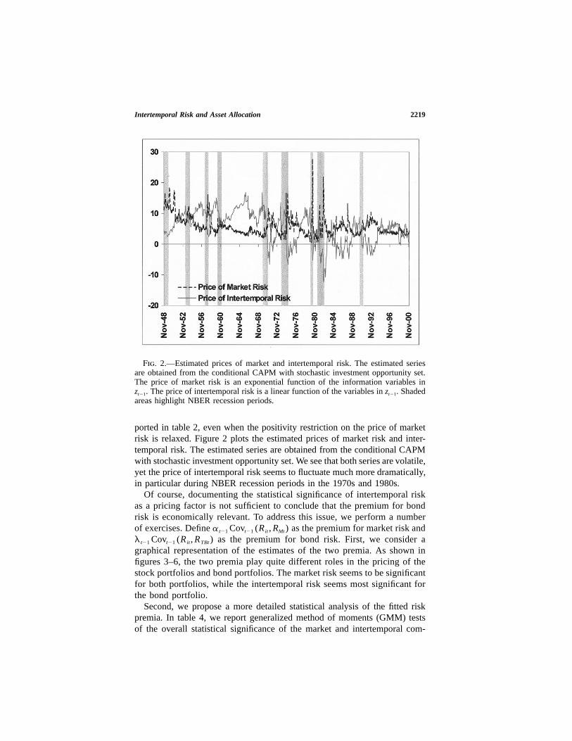
Fig. 2.—Estimated prices of market and intertemporal risk. The estimated seriesare obtained from the conditional CAPM with stochastic investment opportunity set.The price of market risk is an exponential function of the information variables in

The price of intertemporal risk is a linear function of the variables in Shadedz . z .t�1 t�1

areas highlight NBER recession periods.

ported in table 2, even when the positivity restriction on the price of marketrisk is relaxed. Figure 2 plots the estimated prices of market risk and inter-temporal risk. The estimated series are obtained from the conditional CAPMwith stochastic investment opportunity set. We see that both series are volatile,yet the price of intertemporal risk seems to fluctuate much more dramatically,in particular during NBER recession periods in the 1970s and 1980s.

Of course, documenting the statistical significance of intertemporal riskas a pricing factor is not sufficient to conclude that the premium for bondrisk is economically relevant. To address this issue, we perform a numberof exercises. Define as the premium for market risk anda Cov (R , R )t�1 t�1 it Mt

as the premium for bond risk. First, we consider al Cov (R , R )t�1 t�1 it TBt

graphical representation of the estimates of the two premia. As shown infigures 3–6, the two premia play quite different roles in the pricing of thestock portfolios and bond portfolios. The market risk seems to be significantfor both portfolios, while the intertemporal risk seems most significant forthe bond portfolio.

Second, we propose a more detailed statistical analysis of the fitted riskpremia. In table 4, we report generalized method of moments (GMM) testsof the overall statistical significance of the market and intertemporal com-


Fig. 3.—Equity market portfolio: estimated market and intertemporal premiums.Shaded areas highlight NBER recession periods.

Fig. 4.—Long-term Treasury bond portfolio: estimated market and intertemporalpremiums.

ponents of the fitted premia for each asset and for the equity and fixed incomeportfolios jointly. The tests shows that the fitted market risk premiums aresignificantly different from zero for each individual asset and each group ofassets. In contrast, the fitted intertemporal risk premiums are significant forthe fixed income assets only and not for the equity portfolio when each assetis considered individually. However, the fitted intertemporal risk premiumsare significant for equities when the two stock portfolios are considered jointly.

In tables 5 and 6, we provide summary statistics of the prices of market


Fig. 5.—Small stocks portfolio: estimated market and intertemporal premiums.

Fig. 6.—Corporate bond portfolio: estimated market and intertemporal premiums.

and intertemporal risk as well as the estimated total premiums and their com-ponents for the overall sample as well as an analysis of how the prices andpremiums change over time and across business expansions and recessions.Over the entire sample, the average prices of intertemporal risk and of marketrisk are both positive and of similar magnitude. However, the price of inter-temporal risk exhibits twice as much volatility as the price of market risk.The average premium for intertemporal risk is equal to 0.1% and 0.13% permonth for corporate bonds and Treasury bonds, respectively. Arguably, theannualized premiums of 1.3% and 1.5% are also economically relevant, es-pecially considering that the average annualized market risk premiums for


TABLE 4 Statistical Tests on the Fitted Risk Premia

Individual Portfolio Tests 2(x (1))

Market Risk p-value Intertemporal Risk p-value

Market portfolio 122.30 .000 .76 .384Long bonds 13.47 .000 13.65 .000Small stocks 127.10 .000 .37 .546Corporate bonds 27.51 .000 11.42 .001

Joint Tests 2(x (2))

Market Risk p-value Intertemporal Risk p-value

Equity assets 127.11 .000 15.94 .000Bond assets 35.95 .000 13.71 .000

Note.—This table reports GMM tests on the fitted risk premium series to check their difference from zero.Variances are computed using a Bartlett-kernel estimator where the bandwidth is selected according to Andrews(1991). The Newey and West (1987) method is used for serial correlation correction for the standard errors.

these assets were equal to 1.9% and 1.1%, respectively, as documented inpanel B of table 5. Given that the estimated prices of risk are approximatelyequal and that the fixed income portfolios earn premiums of similar magnitudesfor both market and intertemporal risk, we can infer that both bond portfolioshave exposures of similar magnitudes to both market and intertemporal risk.For the market portfolio, the average intertemporal risk premium is 0.015%on a monthly basis. The corresponding market risk premium is 0.989% permonth. These numbers are consistent with the commonly documented marketpremiums. In our case, the average total premium, obtained as the sum of themarket premium and the bond premium (see panel C in table 5) is equal to12% on an annual basis for the market portfolio and 13.2% for small stocks.For these two portfolios, exposure to market risk is several orders of magnitudelarger than to intertemporal risk. The last three columns in tables 5 and 6report joint tests of the hypothesis that the risk premiums are equal to zero.For the average premiums, these tests confirm the results of the tests reportedin table 4.

Tables 5 and 6 also investigate whether the estimated prices of risk andfitted risk premia change over the business cycle (table 5), as well as fromthe first half of the sample period to the second half (table 6). The tests areperformed using a robust dummy variable regression in which the constantrepresents the average premium or price during expansions or during the firsthalf of the sample and the dummy variable coefficient is the estimate of thechange in prices or premiums during NBER recessions or the second half ofthe sample. The results in panel A of table 5 indicate, surprisingly, that thereis no significant change either in the price of intertemporal risk or in the fittedintertemporal risk premiums over the business cycle. Looking at individualassets, the intertemporal risk premiums average to zero during recessions forthe market portfolio, while they become more negative for the small stockportfolio. However, the results in panel B of table 5 suggest that the price ofmarket risk and the fitted market risk premiums increase significantly during


TABLE 5 Decomposition of Total Risk Premiums and the Business Cycle

A. Intertemporal Risk Premium

lt�1 RMt RTBt RSt RCBt2x (eq)2

2x (bnds)22x (all)4

Average 5.17 .015 .126 �.009 .109 15.34 13.72 19.42(.83) (.017) (.052) (.015) (.032) (.000) (.001) (.001)

Cst 5.41 .018 .124 �.005 .108 14.33 20.57 22.40(.89) (.015) (.029) (.013) (.024) (.001) (.000) (.000)

DNBER �1.22 �.019 .013 �.022 .004 .32 .25 .69(1.34) (.054) (.089) (.047) (.097) (.853) (.884) (.952)

B. Market Risk Premium

at�1 RMt RTBt RSt RCBt2x (eq)2

2x (bnds)22x (all)4

Average 5.57 .989 .092 1.125 .161 153.5 40.56 159.4(.41) (.081) (.021) (.091) (.027) (.000) (.000) (.000)

Cst 5.26 .891 .074 1.011 .131 156.7 70.56 156.7(.33) (.075) (.016) (.082) (.019) (.000) (.000) (.000)

DNBER 2.13 .586 .110 .678 .179 9.09 5.64 10.75(.79) (.195) (.063) (.223) (.077) (.011) (.060) (.030)

C. Total Risk Premium

RMt RTBt RSt RCBt2x (eq)2

2x (bnds)22x (all)4

Average 1.004 .218 1.115 .269 165.8 95.96 276.5(.079) (.026) (.091) (.028) (.000) (.000) (.000)

Cst .909 .198 1.005 .239 156.0 143.8 327.4(.073) (.023) (.083) (.020) (.000) (.000) (.000)

DNBER .567 .122 .656 .184 9.28 7.11 16.23(.187) (.055) (.220) (.071) (.010) (.029) (.003)

Note.—The table reports summary statistics of the prices of intertemporal and market risk, as well as ofthe estimated risk premia and tests of whether the estimated prices and premiums differ between NBERrecessions and expansions. The tests are performed by regressing the estimated prices and premiums on aconstant and a dummy variable taking a value of 1 during NBER recessions. We compute the testsCst DNBER

for the following three risk premiums:

ˆ ˆIntertemporal premium : q p l Cov (R , R ),it t�1 t�1 it TBt

ˆ ˆMarket premium : f p a Cov (R , R ),it t�1 t�1 it Mt

ˆ ˆˆTotal premium : h p a Cov (R , R ) � l Cov (R , R ).it t�1 t�1 it Mt t�1 t�1 it TBt

Tests of whether the estimated premiums are jointly significant for the equity assets, the fixed income assets,and all assets simultaneously are reported in the last three columns. All standard errors (in parentheses) arecomputed using a Bartlett-kernel estimator with bandwidth selected according to Andrews (1991) and Neweyand West (1987) serial correlation correction.

recessions. This is true also for the fixed income portfolio, although the jointtest that the fitted market premium for bond portfolios increases in recessionsis only significant at the 6% level. Panel C indicates that the resulting increasein total premiums during recessions is significant across the board. In partic-ular, the total premiums on all assets are approximately 60% higher duringNBER recessions than during expansions.

The changes in the fitted prices and premiums from the first half of thesample to the second half are reported in table 6. One notices immediatelythe significant decrease in the prices of both intertemporal risk and marketrisk over the second half of the sample period. The average price of inter-temporal risk decreases by 75%, while the price of market risk decreases by20%. The decrease in the price of intertemporal risk induces a substantial


TABLE 6 Decomposition of Total Risk Premiums: Subsample Evidence

A. Intertemporal Risk Premium

lt�1 RMt RTBt RSt RCBt2x (eq)2

2x (bnds)22x (all)4

Average 5.17 .015 .126 �.009 .109 15.34 13.72 19.42(.83) (.017) (.052) (.015) (.032) (.000) (.001) (.001)

Cst 8.41 .006 .172 �.017 .126 9.60 32.33 33.31(.81) (.017) (.038) (.018) (.023) (.008) (.000) (.000)

DPost�1973 �6.12 .017 �.090 .015 �.033 .274 7.89 8.59(1.21) (.034) (.065) (.030) (.062) (.853) (.019) (.072)

B. Market Risk Premium

at�1 RMt RTBt RSt RCBt2x (eq)2

2x (bnds)22x (all)4

Average 5.57 .989 .092 1.125 .161 153.5 40.57 159.4(.41) (.081) (.021) (.091) (.027) (.000) (.000) (.000)

Cst 6.21 .937 .035 1.101 .093 69.75 35.69 128.2(.63) (.116) (.017) (.134) (.025) (.000) (.000) (.000)

DPost�1973 �1.19 .100 .110 .045 .132 8.72 9.05 21.85(.67) (.161) (.037) (.182) (.048) (.013) (.011) (.000)

C. Total Risk Premium

RMt RTBt RSt RCBt2x (eq)2

2x (bnds)22x (all)4

Average 1.004 .218 1.115 .269 165.8 95.96 276.5(.079) (.026) (.091) (.028) (.000) (.000) (.000)

Cst .943 .208 1.084 .218 66.61 62.39 107.67(.118) (.034) (.138) (.028) (.000) (.000) (.000)

DPost�1973 .117 .021 .060 .098 11.95 8.05 30.86(.155) (.051) (.181) (.051) (.003) (.018) (.000)

Note.—The table reports summary statistics of the prices of intertemporal and market risk, as well as ofthe estimated risk premia and tests of whether the estimated prices and premiums differ between the first andsecond half of the sample period. The tests are performed by regressing the estimated prices and premiumson a constant and a dummy variable taking a value of 1 after December 1973. We compute theCst DPost-1973

tests for the following three risk premiums:

ˆ ˆIntertemporal premium : q p l Cov (R , R ),it t�1 t�1 it TBt

ˆ ˆMarket premium : f p a Cov (R , R ),it t�1 t�1 it Mt

ˆ ˆˆTotal premium : h p a Cov (R , R ) � l Cov (R , R ).it t�1 t�1 it Mt t�1 t�1 it TBt

Tests of whether the estimated premiums are jointly significant for the equity assets, the fixed income assets,and all assets simultaneously are reported in the last three columns. All standard errors (in parentheses) arecomputed using a Bartlett-kernel estimator with bandwidth selected according to Andrews (1991) and Neweyand West (1987) serial correlation correction.

reduction in the fitted intertemporal risk premiums for the fixed income port-folio, which, although not significant for the individual portfolios, is highlysignificant jointly. The equity portfolios intertemporal risk premiums increaseduring the second half of the sample, although not significantly. Turning tothe fitted market risk premiums in panel B of table 6, we see that the priceof market risk decreased in the post-1973 period and that the fitted marketrisk premiums uniformly increased. Even though these increases are not al-ways significant at the individual portfolio level, the tests reported in the lastthree columns of the table indicate that the market premium increases arejointly significant for the equity portfolios, the bond portfolios, and all assets


simultaneously. For the total premiums, although the joint tests suggest asignificant change from the pre- to the post-1973 period, the total premiumchange on individual assets is small and insignificant.

To summarize, we find that the prices of both market risk and intertemporalrisk are significant and time varying. Further, we find that the fitted market riskpremia and the intertemporal risk premia both are statistically and economicallysignificant for equity and fixed income portfolios, although intertemporal riskpremia represent a much larger fraction of total risk premia for bond portfoliosthan for equity portfolios. Moreover, we find that total fitted risk premiumstend to increase during NBER recessions and that increase is driven mainlyby a significant increase of the price of market risk. Finally, we document asignificant decrease in the price of both sources of risk in the post-1973 period.However, although the prices of risk decrease, estimated total premiums in-crease due to increased levels of risk. Our tests suggest that both market riskand intertemporal risk are important risk factors in the pricing of financialassets. Finally, we would like to note that, although we find evidence sup-porting the importance of an intertemporal hedge factor to price risky assets,our investigation in no way precludes the existence of additional priced factors.

VI. Intertemporal Asset Allocation and Hedging

To assess further the economic importance of intertemporal risk, we examineits effect on investors’ portfolios. In this section, we investigate the gains thatmay arise from explicitly considering intertemporal risk in the asset allocationdecision. In the next section, we explore the dynamics of the market risk andintertemporal risk premiums and their links with business cycles by investi-gating the properties of two specific portfolios.

A. Optimal Portfolio Weights

Our empirical analysis yields conditional expected returns and conditionalcovariances for the four asset classes. Consider an investor who faces marketrisk as well as intertemporal risk in her asset allocation decision. This investorcan proceed in several ways. She could construct an optimal portfolio thatincludes equity assets only. She could decide to hedge her equity portfolioagainst intertemporal risk. Or she could invest in a portfolio that includes bothequity and fixed income assets to optimally manage her exposure to marketrisk and intertemporal risk.

Assume that investors maximize the expected utility of future consumption.The investment opportunity set, available to all investors, includes the fol-lowing securities:

• two risky equity assets, that is, a market index portfolio and a smallstocks portfolio. Given that we know the composition of the marketportfolio, this is equivalent to the two equity asset classes of large andsmall stocks;


• two risky bond assets, that is, the corporate bonds portfolio and the long-term T-bonds portfolio.

Each investor has access to a total of four ( ) risky securities and oneN p 4risk-free asset (the 1-month Treasury bill). Let g denote the investor’s degreeof risk aversion. Also, indicate with m the ( ) vector of expected returnsN # 1in excess of the risk-free rate on the N risky assets, and with S the ( )N # Ncovariance matrix for the risky assets. Mean-variance optimization implies thefollowing portfolio allocation:

�11 1 q S m 0N p � 1 � , (9) ′ �1 ( )q 1 � i S m 1g g N�1

where is the ( ) vector of optimal weights for the risky assets,q N # 1 NN

is the fraction of the portfolio invested in the risk-free asset, and i is aqN�1

vector of ones.The optimal weights in equation (9) deserve further discussion. Consider an

investor with a logarithmic utility function. This would be equivalent to theassumption that . In this case, the portfolio weights in (9) simplify intog p 1

�1 q S mN p , (10) ′ �1q 1 � i S m N�1

where is the vector of optimal weights for the N risky assets. The�1q p S mN

portfolio in equation (10) is common among all investors and is usually�1S m

referred to as the universal logarithmic portfolio. Investors with any degreeof risk aversion g would just scale their investment in the logarithmic portfolioby by shifting funds to or from the risk-free asset.1/g

Our discussion to this point implies that all investors hold a combinationof two portfolios: the universal portfolio of risky assets and the risk-free asset.The allocation between the two depends on the degree of risk aversion ofeach investor. Specifically, investors exploit the correlation structure for theentire set of available assets and choose an allocation that maximizes theSharpe ratio of their portfolio. This result is similar to the standard solutionof a portfolio problem. However, when investors have access to long-termbond markets, the result has a number of additional implications, which canbe derived after appropriately partitioning both m and S:17

m S Ss ss sdm p Sp , m S S d ds dd

where the letter s denotes the stock portfolios and the letter d indicates thebonds portfolios (long-term corporate bonds and long-term Treasury bonds).The bonds can be held both for speculative and/or hedging purposes.

Define the matrix of coefficients from the regression�1G p S S , [2 # 2]dd ds

17. A similar partitioning is used by Glen and Jorion (1993) and Jorion and Khoury (1995)to discuss the implications of optimal currency hedging on international portfolio performance.


of the stock returns on the bond returns. Also define the′S p S � G S G,s/d ss dd

( ) covariance matrix of the stock returns, conditional on the bonds.2 # 2Hence, is the covariance matrix of fully hedged equity returns. StandardSs/d

rules from the inversion of a partitioned matrix imply the following result:

�1 �1 ′ �1 ′ q S m � S G m S (m � G m )s �1 s/d s s/d d s/d s dpS m p p , (11) �1 �1q S m � Gq S m � Gq d dd d s dd d s

where and are the vectors of optimal weights for, respectively, the equitiesq qs d

and the bonds included in the universal portfolio. The first interesting featureof equation (11) is that the optimal choice of and should be madeq qs d

simultaneously to exploit the properties of both sets of asset classes. Theequity positions are a function of the covariance of the fully hedged stockreturns and mean equity returns adjusted for the cost of the hedge. The bondpositions have two components. The expression is the solution to a�1S mdd d

standard mean-variance problem for the optimal portfolio of bonds only and,therefore, can be interpreted as a purely speculative position in bonds. On theother hand, the expression reflects the investment in bonds that minimizesGqs

the variance of the portfolio given the position in equities. In this sense,investors hold bonds for both speculative and hedging purposes.18

Two special cases are of interest. First, if the expected excess returns onbonds are zero, then the optimal portfolio weights simplify to

�1 q S ms �1 s/d spS m p . (12) q �Gq d s

In this case, the optimal strategy calls for selecting equity portfolio weightsbased not on the equity unhedged expected returns but on the covariancematrix of their fully hedged returns. However, the bond positions have onlya hedging component. If the intertemporal risk is fully diversifiable, then

and and the optimal portfolio includes only equity posi-�1 �1G p 0 S p Ss/d ss

tions. It is also the solution to a standard mean-variance problem for theoptimal portfolio of unhedged equity investments.

Our empirical exercise focuses on three dynamic strategies of particularinterest: investing each month in the overall optimal portfolio, investing inan optimal portfolio of equities only, or investing in equities and hedgingintertemporal risk. Our discussion of optimal portfolio choice will help identifythe shortcomings of each strategy and the circumstances under which theymay be optimal. Using the notation introduced above, the three strategies canbe summarized as follows:19

18. The expression for is equivalent to the expression for the optimal hedge for a prespecifiedqd

portfolio derived in Anderson and Danthine (1981); as they show, this would be valid for anychoice of .qs

19. Implicitly, the weights in the table assume that the investor has a degree of relative riskaversion of 1. It is a simple matter to scale the portfolio weights of the risky assets by the inverseof the degree of relative risk aversion to get the optimal weights for any level of risk aversion.


Portfolio Position

Equities Long-Term Bonds

1. EO �1q p S ms ss s q p 0d

2. EO � IH �1q p S ms ss s q p �Gqd s

3. OPT �1 �1 ′q p S m � S Gs s/d s s/d md

�1q p S m � Gqd dd d s

1. Optimal equity-only strategy(EO): In this strategy, we take the point ofview of a manager whose mandate prohibits her from taking direct positionsin long-term bonds. She optimizes her portfolio holdings over the eligibleequity positions only. This strategy would be optimal only if the intertemporalrisk exposure of the equity investments is fully diversifiable and bonds havezero expected excess returns.

2. Overlay intertemporal hedge strategy( ): This strategy corre-EO � IHsponds to the situation where the role of an equity portfolio manager is distinctfrom the role of a bond manager. First, the equity portfolio manager choosesher optimal equity portfolio weights in the same fashion as in strategy 1.Second, conditional on these equity portfolio weights, the plan sponsor op-timally hedges her exposure to the intertemporal risk. This implicitly assumesthat intertemporal risk commands a zero premium, and hence no speculativeposition in bond assets is allowed. However, the equity allocation is suboptimalsince the equity positions are selected without taking into account the cor-relations between equity and bond assets.

3. Overall optimal allocation[OPT]: This strategy implements the unre-stricted global optimum portfolio strategy. The portfolio weights of equityand bond assets are selected simultaneously, taking into account the covari-ances between all assets. In particular, the equity positions now reflect theircovariance with the bond assets and the costs of the minimum variance hedges.

Note that the bond positions are always determined as a function of thepositions in the equity portion of the portfolio. Hence, we can evaluate thebenefits of overlay strategies for any given portfolio of equities as long aswe have estimates of the excess returns on bonds and of the variance-co-variance matrix of the equity and bond assets considered.

B. Portfolio Performance

We implement each strategy at the beginning of each month and record itsperformance and characteristic over the whole sample period. We use ourestimated model to provide beginning-of-month forecasts of expected returnsand volatility. Note that time variation in the price of market risk reflects timevariation in the aggregate degree of relative risk aversion in the economy. Allthe strategies are scaled by one over the estimated relative risk aversioncoefficient. Table 7 summarizes the performance and characteristics of thethree portfolio strategies described in the preceding subsection. We also reportthe characteristic of the minimum variance hedge for the equity-only portfolio,


TABLE 7 Optimal Strategies Characterisitcs

OverallOptimalPortfolio

Equity-Only

PortfolioOverallHedge

HedgedEquity-Only

Portfolio

MinimumVarianceHedge

Fraction in Risky Fund

Mean .472 .930 �.458 .960 .030SD .443 .181 .486 .158 .108

Realized Excess Returns

Mean .933 .842 .091 .569 �.273SD 4.964 5.750 5.380 3.731 4.370Minimum �24.635 �23.72 �12.52 �25.20 �10.52Maximum 32.31 14.94 34.67 11.93 7.55Sharpe Ratio .188 .146 .017 .152 �.062

Correlations of Realized Excess Returns

Optimal portfolio (OPT) 1.000Equity-only portfolio (EO) .810 1.000Optimal hedge .384 �.604 1.000EO � IH portfolio .776 .650 .021 1.000Maximum variance hedge �.000 �.761 .813 �.001 1.000

Expected Excess Returns

Mean .978 .724 .254 .663 �.061E[SD] 4.600 4.013 2.587 3.660 1.694Minimum .136 .015 �4.635 .000 �7.704Maximum 7.269 7.713 3.144 5.776 1.030

Note.—This table reports the performance and characteristiscs of dynamic portfolio strategies. We considerthree portfolio strategies: the overall optimal portfolio of all assets (OPT), the optimal portfolio restricted toequity only (EO), and the optimal equity-only portfolio hedged for intertemporal risk (EO�IH). Overall hedgereports the difference in portfolio characteristics between the overall optimum and the equity-only portfolioand can be thought of as a proxy for an overall optimum intertemporal hedge portfolio. Minimum variancehedge reports the mimimum variance intertemporal hedge for the equity-only portfolio. Expected returns andcovariances are the fitted values from our general model. All returns are reported in percent per month.

as well as the difference between the equity-only and global optimal portfolios.We use the last one as our proxy for the optimal intertemporal hedge portfolio.

We first report the fraction of the overall portfolios invested in the fourrisky assets. For the equity-only optimal portfolio, on average 93% of theoverall portfolio is invested in the two equity assets, the rest being investedin the riskless asset. The standard deviation of the fraction in the risky assetis 18%, which represents a rough measure of average monthly turnover. Bycomparison, the global optimal portfolio has 47% of assets in risky funds anda standard deviation of 44%. The minimum variance hedge of the equity-onlyportfolio has a substantially smaller impact on the fraction in risky assets.While the minimum variance hedge decreases both the returns and volatilityof the equity only portfolio, leaving the portfolio realized Sharpe ratio basicallyunchanged, the global optimal hedge induces both higher returns and lowervolatility in the global optimum portfolio than in the equity-only optimumportfolio. The realized monthly Sharpe ratio is 0.146 for the equity-onlyportfolio and 30% higher at 0.188 for the global optimum portfolio. To put


Fig. 7.—In sample performance of dynamic strategies. This figure plots the cu-mulative returns on three strategies: (a) overall optimal portfolio, (b) optimal equity-only portfolio, and (c) optimal equity-only portfolio hedged against intertemporal risk.

these numbers in perspective, a portfolio of the risk-free asset and the optimumequity-only portfolio with a volatility equal to the realized volatility of theglobal optimum portfolio would have earned a 0.727% mean premium permonth compared to a realized mean premium of 0.933% for the global op-timum. Hence, for the global optimum, out of an annual average excess returnof 11.20%, 2.47%, or a bit more than a fifth, can be directly traced back tothe optimal consideration of intertemporal risk in the portfolio optimizationprocess. The performance of the different strategies is also illustrated in figure7, which plots the cumulative total returns of the three strategies from October1948 to December 2000.

The correlations across the different portfolios are reported in the thirdpanel of table 7. First, we see that the reason why combining the optimalhedge with the equity-only portfolio yields a superior risk-reward trade-offfor the global optimum portfolio is the very large negative correlation of�0.604 between the two portfolios. Second, not surprisingly, the minimumvariance hedge for the equity-only portfolio yields a position with even lowerrealized correlation of �0.761 with that portfolio. These realized correlationsalso confirm that our approach indeed identifies hedge portfolios. Finally, thefourth panel reports the average expected mean excess return and the averageexpected volatility for all the strategies and hedge portfolios. For all three,strategies expectations and realizations of mean returns and volatility are not


far apart. For both hedge portfolios, however, expectations and realizationsdepart more substantially.

In summary, we find that the global hedge portfolio exhibits a significantnegative correlation of �0.604 with the equity-only portfolio. Although earn-ing only a small positive 1.1% annual excess return and having a volatilityof similar magnitude as the equity-only portfolio, the global hedge significantlyimproves the risk-reward trade-off of the global optimal portfolio: it accountsfor 22% of the global optimal portfolio risk premium, or approximately anadditional 2.5% annual premium.

VI. The Importance of Intertemporal Risk

In this section, we explore the dynamics of the market and intertemporal riskpremiums and their links with business cycles by investigating the propertiesof two specific portfolios. These portfolios are constructed to yield the max-imum Sharpe ratios among all portfolios with zero exposure to either inter-temporal risk or market risk. Specifically, we construct efficient frontiers ofportfolios that are orthogonal to intertemporal risk or market risk.

A. Portfolios Orthogonal to Intertemporal Risk

To hedge completely against the intertemporal risk, an investor is constrainedto invest in portfolios orthogonal to the long-term Treasury bond portfolio,

′q Sq p 0, (13)Z b

where

′q p [0 0 1 0]b

is the vector of portfolio weights for the Treasury bond portfolio and qZ

represents the weights for all the portfolios orthogonal to the Treasury port-folio. Roll (1980) shows that, for a portfolio that is off the mean-varianceefficient frontier, the set of portfolios orthogonal to it is given by an areabounded by a quadratic function. Figure 8 illustrates the set of orthogonalportfolios. Point b represents the intertemporal risk portfolio proxied by thelong-term Treasury bond portfolio. If we draw a line from the intertemporalrisk portfolio through the global minimum variance portfolio, we find theexpected return of the minimum variance portfolio orthogonal to the in-z0

tertemporal risk. The hatched area represents the set of portfolios orthogonalto the intertemporal risk. We minimize the variance of portfolios subject toconstraint (13) to find the risky asset weights for the orthogonal mean-variancefrontier,

�1 �1 �1 ′q p [q : S m : S i]H [0 : m : 1]Z b z

′{ M[0 : m : 1] , (14)z

where is the mean excess return of the orthogonal portfolio and is am Hz


Fig. 8.—Constrained efficient frontier for portfolios orthogonal to the long-termTreasury portfolio. This figure shows the set of portfolios orthogonal to the long-termTreasury portfolio. The Sharpe ratios of the fully efficient frontier and the constrainedefficient frontier are indicated by the two lines from the origin to the tangencies onthe the frontiers.

matrix of the following form:(3 # 3)

′ �1H p [Sq : m : i] S [Sq : m : i]b b

2 j m 1b b′ �1 ′ �1p m m S m m S i .b ′ �1 ′ �11 m S i i S i

The efficient portfolio frontier for the orthogonal portfolios is then a straightline from the origin to the tangency on the hatched region. It is apparent thatthe constrained efficient frontier is dominated by the fully efficient frontier.

There are two ways that we can examine the relative importance of theintertemporal risk. First, we can study the time series absolute and relativedifferences in the Sharpe ratios. The Sharpe ratios for any constrained orunconstrained efficient frontier portfolio q can be computed as

′q mSRp .′�q Sq

The Sharpe ratio for the overall efficient frontier is just the Sharpe ratio forthe overall tangency portfolio. For the orthogonal frontier, the expected excess


return of the tangency portfolio is

′�M SM3 3∗m p ,z ′M SM2 3

where and are the second and third columns of M defined above inM M2 3

equation (14). By substituting into equation (14), we obtain the weights∗mz

for the tangency portfolio and Sharpe ratios can be computed. We can testwhether the Sharpe ratios for the fully efficient frontier and the orthogonalfrontier are statistically different.

The second way to study the relative importance of the intertemporal riskis to analyze the difference in excess returns for a fixed level of portfolio riskand derive implications for the cost of hedging or the benefits of taking intoaccount the intertemporal risk. We can quantify the cost or benefit in termsof premiums.

As a comparison, we also conduct the above exercises with respect to themarket risk. The mathematics for the portfolio frontier orthogonal to the marketrisk is similar to that to the intertemporal risk. We simply use

′q p [1 0 0 0]b

instead of

′q p [0 0 1 0]b

in deriving the weights for the optimal orthogonal portfolios.

B. Empirical Evidence

Using the estimated conditional means and covariances of the four assets, weapply the constrained mean variance analysis derived above and compute theconditional Sharpe ratios of various portfolios. Figures 9 and 10 plot optimalSharpe ratios over the entire sample for three types of strategies. The unhedgedportfolio represents the tangency portfolio for the overall mean-variance frontier.Figure 9 graphs the Sharpe ratios for the unhedged portfolio with those fromportfolios hedged against intertemporal risk, that is, the tangency portfolios fromthe frontier orthogonal to the intertemporal risk. The result is striking. We findthat the unhedged Sharpe ratios coincide with the intertemporal risk-hedgedSharpe ratios during most periods in the sample, except from 1956–1961,1969–1970, 1978–1982, and 1988–1990. These periods occur before or duringrecessionary periods.

In contrast, figure 10 graphs the Sharpe ratios for the unhedged portfoliowith those from portfolios hedged against market risk, that is, the tangencyportfolios from the frontier orthogonal to the market risk. The difference inSharpe ratios for these two strategies is large and volatile throughout the entiresample. There is nothing special in terms of the difference in Sharpe ratioduring the above-mentioned periods. In fact, the difference in Sharpe ratio is


Fig. 9.—Expected Sharpe ratios on optimal unhedged and intertemporal-risk hedgedportfolios. This figure plots the Sharpe ratios of an unconstrained efficient portfolioand the constrained efficient portfolios orthogonal to market risk. Shaded areas high-light NBER recession periods.

Fig. 10.—Expected Sharpe ratios on optimal unhedged and market-risk hedgedportfolios. This figure plots the Sharpe ratios of an unconstrained efficient portfolioand the constrained efficient portfolios orthogonal to market risk. Shaded areas high-light NBER recession periods.


large and relatively stable outside those periods. For example, during the1990s, the loss in Sharpe ratio by hedging against the market risk is consis-tently high and ranges between 0.05 and 0.31. These two graphs indicate thatthe cost of hedging against intertemporal risk is generally low, except duringadverse market conditions. This may reflect the fact that the benefit of hedgingagainst intertemporal risk is also low during normal market conditions. Thecost of hedging against market risk, however, is shown to be very significantduring the entire sample. The cost seems to be smaller and more volatileduring the 1978–82 period, suggesting some benefit of hedging against marketrisk during severe market conditions.

One may argue that the conditional Sharpe ratios do not reflect the realizedperformance of the strategies. To answer this question, we also compute “realizedSharpe ratios” using realized excess returns under the three strategies. Figures11 and 12 plot the difference in the expected (conditional) and realized Sharperatios between an unconstrained efficient portfolio and the constrained efficientportfolios orthogonal to either intertemporal or market risk. The realized dif-ferences in Sharpe ratio are certainly much more volatile, but overall they seemto vary around the expected differences.

Certainly, Sharpe ratios may not be a good measure of cost of hedging againsta particular risk. Another measure is the difference in risk premium for a commonbenchmark risk level. We next compute expected risk premiums on unconstrai-ned efficient portfolios (OPT) and on efficient portfolios either orthogonal tomarket (OPTHMR) or intertemporal risk (OPTHIR). The portfolios are con-structed to have volatilities equal to the average market portfolio volatility duringNBER recessions and to the average market volatility during NBER expansions.Table 8 reports summary statistics of these risk premiums. The last two columnsof that table report the additional premium earned for bearing market risk orintertemporal risk when comparing the unconstrained optimal portfolio and theefficient portfolios orthogonal to market or intertemporal risk (MktRP pOPT � OPTHMR; IntRP p OPT � OPTHIR).

The average estimated risk premium for bearing intertemporal risk is 0.331%per month, which translates into a 4.0% annual risk premium. During NBERmarket expansion, the monthly intertemporal risk premium is 0.300% (3.6%annually), while during recession, the premium is 0.186% per month higher at0.486% (5.8% annually). The mean difference between risk premiums for theunconstrained optimal portfolio and the efficient portfolios hedged against theintertemporal risk is 0.118% per month (1.4% annually). This implies that theincremental reward of bearing optimal amounts of intertemporal risk in additionto market risk is 1.4% annually. During expansion, this risk premium is 0.091%per month (1.1% annually), while during recession this premium increases by0.160% to 0.251% per month (3.0% annually). Therefore, intertemporal risk isoverall significant for asset allocation decisions, especially during down marketsand business recessions.20

20. Ang and Bekaert (2004) show that, during a persistent bear market, investors tend to switch


Fig. 11.–Difference in Sharpe ratios between the unconstrained opitmal portfolioand the constrained optimal portfolio orthogonal to intertemporal risk. Shaded areashighlight NBER recession periods.

Fig. 12.—Difference in Sharpe ratios between the unconstrained opitmal portfolioand the constrained optimal portfolio orthogonal to market risk. Shaded areas highlightNBER recession periods.


TABLE 8 Decomposition of Optimal Portfolios Risk Premiums and theBusiness Cycle

OPT OPTHIR OPTHMR MktRP IntRP

Average .874 .756 .331 .543 .118(.062) (.060) (.034) (.063) (.063)

Expansion .774 .683 .300 .474 .091(.049) (.050) (.031) (.055) (.021)

D Recession .594 .434 .186 .408 .160(.152) (.157) (.069) (.155) (.071)

Due to DSRt .514 .363 .155 .359 .151(.153) (.158) (.070) (.155) (.071)

Due to DjM .080 .071 .031 .049 .009(.005) (.005) (.003) (.005) (.002)

Note.—The table reports summary statistics of expected risk premiums on unconstrained efficient portfolios(OPT) and on efficient portfolios either orthogonal to market (OPTHMR) or intertemporal risk (OPTHIR). Thelast two columns report the incremental premiums earned for bearing market risk or intertemporal risk whencomparing the unconstrained optimal portfolio and the efficient portfolios orthogonal to market or intertemporalrisk ( ). The portfolios are constructed to have volatilitiesMktRP p OPT � OPTHMR; IntRP p OPT � OPTHIRequal to the recession average market portfolio volatility during NBER recessions and to the expansion averagemarket volatility during NBER expansions. We test whether the estimated premiums differ between NBERrecessions and expansions and whether the change in premium is due to change in Sharpe ratios or in marketvolatility. Risk premiums are reported in percent per month. All standard errors (in parentheses) are computedusing a Bartlett-kernel estimator with bandwidth selected according to Andrews (1991) and Newey and West(1987) serial correlation correction. The row “D Recession” indicates increases in risk premium during NBERrecessions.

In comparison to intertemporal risk, the average estimated risk premium forbearing market risk is 0.756% per month, or 9.1% on an annual basis. DuringNBER market expansion, the monthly market risk premium is 0.683% (8.2%annually), while during recession, the premium is 0.434% per month higher at1.112% (13.4% annually). The mean difference between risk premiums for theunconstrained optimal portfolio and the efficient portfolios hedged against themarket risk is 0.543% per month (6.5% annually). This implies that the incre-mental reward of bearing optimal amounts of market risk in addition to inter-temporal risk is 6.5% annually. During expansions, this risk premium averages0.474% per month (5.7% annually), while during recessions it increases by0.408% to 0.882% per month (10.1% annually). Not surprisingly, market riskis a more significant risk than intertemporal risk for asset allocation decisions.

Figures 13 and 14 plot the difference between the expected premium earnedon an unconstrained efficient portfolio and on efficient portfolios fully hedgedagainst intertemporal (fig. 13) or market risk (fig. 14). We see that, in terms ofrisk premiums, the cost of hedging the market risk is very high, averaging0.543% per month, as compared to an average of 0.118% per month for hedgingagainst intertemporal risk. Yet intertemporal risk can be important. For example,during the 1978–82 period, intertemporal risk premium reached a high of 2.8%per month (33.6% per year).

to all-cash investment. This may reflect the need for hedging during adverse market conditions.Our findings indicate that investors demand more intertemporal hedging and are willing to paya higher premium for such hedging during recessions.


Fig. 13.—Difference in expected premiums between the unconstrained optimal port-folio and the optimal portfolios fully hedged against intertemporal risk. The portfoliosare chosen to have a volatility equal to the recession average market portfolio volatilityduring NBER recesssions and to the expansion average market volatility during NBERexpansions. Shaded areas highlight NBER recession periods.

Fig. 14.—Difference in expected premiums between the unconstrained optimal port-folio and the opotimal portfolios fully hedged against market risk. The portfolios arechosen to have a volatility equal to the recession average market portfolio volatilityduring NBER recessions and to the expansion average market volatility during NBERexpansions. Shaded areas highlight NBER recession periods.


VIII. Conclusions

In this article, we analyze the statistical and economic relevance of intertem-poral risk in explaining the dynamics of the premium for holding stocks andbonds. We jointly estimate and test a conditional asset pricing model thatincludes long-term interest rate risk as a potentially priced factor for fourbroad classes of assets—large stocks, small stocks, long-term Treasury bonds,and corporate bonds. For the conditional CAPM, we find that market risk—measured by the conditional variance of the return on the market portfolio—is priced and that the reward-to-risk ratio for holding the market (i.e., theprice of market risk) is time varying. We also find that the premium for longbond risk is the main component of the risk premiums of Treasury bond andcorporate bond portfolios, while it represents a small fraction of total riskpremiums for equities. Our results suggest that investors perceive stocks ashedges against variations in the investment opportunity set.

Since the four asset classes under study represent some of the most importantfor investors, we proceed to use our estimated premiums and covariances tocompute the dynamic optimal asset allocations for investors with differentrisk preferences and trading strategies. We use two alternative approaches todecompose portfolio holdings into their hedging and speculative components.First, we construct period by period the equity-only optimal portfolio, theminimum variance intertemporal risk hedge for the equity-only portfolio, andthe global optimal portfolio. To proxy for the optimal intertemporal hedgeportfolio, we use the difference between the equity-only and global optimalportfolios. Although earning only a small premium of 1.1% per year andhaving a volatility of similar magnitude as the equity-only portfolio, the globalhedge significantly improves the risk-reward trade-off of the global optimalportfolio due to its significant negative correlation of �0.604 with the equity-only portfolio. The intertemporal hedge accounts for 22% of the global optimalportfolio risk premium, or approximately 2.5% out of the 11.1% annualpremium.

Second, we construct period by period both the optimal portfolio orthogonalto market risk and the optimal portfolio orthogonal to intertemporal risk. Theperformance of the portfolio orthogonal to market risk provides direct insightsinto the rewards for market-neutral strategies bearing only intertemporal risk.We find that, at average market volatility levels, bearing intertemporal riskonly yields an annual premium of 3.6% during expansion, increasing to 5.8%during recessions. However, the incremental reward of bearing optimalamounts of intertemporal risk in addition to market risk varies between 1.1%per annum during expansions and 3% during recessions.

In sum, our evidence suggests that considering intertemporal risk is im-portant both for asset pricing and for asset allocation decisions, especially tomodel changes in the risk-return trade-off between business recessions andexpansions. Not only does intertemporal risk bear economically meaningfultime-varying premiums but explicitly incorporating intertemporal risk con-


siderations in portfolio decisions brings large benefits, especially during downmarkets.

References

Anderson, Ronald W., and Jean–Pierre Danthine. 1981. Cross hedging. Journal of Political Economy89:1182–96.

Andrews, Donald W. K. 1991. Asymptotic normality of series estimators for nonparametric andsemiparametric regression models. Econometrica59:307–45.

Ang, Andrew, and Geert Bekaert. 2004. How do regimes affect asset allocation? FinancialAnalysts Journal60, no. 2:86–99.

Backus, David K., and Allan W. Gregory. 1993. Theoretical relations between risk premiumsand conditional variances. Journal of Business and Economic Statistics11:177–85.

Baillie, Richard T., and Ramon P. De Gennaro. 1990. Stock returns and volatility. Journal ofFinancial and Quantitative Analysis25:203–14.

Bekaert, Geert, and Guojun Wu. 2000. Asymmetric volatility and risk in equity markets. Reviewof Financial Studies13:1–42.

Berndt, E. K., B. H. Hall, Robert E. Hall, and Jerry A. Hausman. 1974. Estimation and inferencein nonlinear structural models. Annals of Economic and Social Measurement3:653–65.

Black, Fisher. 1972. Capital market equilibrium with restricted borrowing. Journal of Business45:444–54.

Bollerslev, Tim, Robert F. Engle, and Jeffrey M. Wooldridge. 1988. A capital asset pricing modelwith time-varying covariances. Journal of Political Economy96:116–31.

Bollerslev, Tim, and Jeffrey M. Wooldridge. 1992. Quasi-maximum likelihood estimation andinference in dynamic models with time-varying covariances. Econometric Reviews11:143–72.

Boudoukh, Jacob, Matthew Richardson, and Tom Smith. 1993. Is the ex-ante risk premiumalways positive? A new approach to testing conditional asset pricing models. Journal ofFinancial Economics34:387–408.

Brandt, Michael W., and Qiang Kang. 2004. On the relationship between the conditional meanand volatility of stock returns: A latent VAR approach. Journal of Financial Economics72:217–57.

Brennan, Michael J., Ashley W. Wang, and Yihong Xia. 2004. Estimation and test of a simplemodel of intertemporal capital asset pricing. Journal of Finance59:1743–75.

Campbell, John Y. 2000. Asset pricing at the millennium. Journal of Finance55:1515–67.Campbell, John Y., Y. Lewis Chan, and Luis M. Viceira, 2003. A multivariate model of strategic

asset allocation. Journal of Financial Economics67:41–80.Campbell, John Y., and Ludger Hentschel. 1992. No news is good news: An asymmetric model

of changing volatility in stock returns. Journal of Financial Economics31:281–318.Chen, Joseph. 2003. Intertemporal CAPM and the cross-section of stock returns. Unpublished

manuscript, Marshall School of Business, University of Southern California.Chen, Nai-Fu, Richard Roll, and Stephen A. Ross. 1986. Economic forces and the stock market.

Journal of Business59:383–403.Cochrane, John H. 1999 New facts in finance. Economic Perspectives23, no. 3:36–58.De Santis, Giorgio, and Bruno Gerard. 1999. Conditional asset pricing with market and inflation

risk. Working paper, Anderson School, University of California, Los Angeles.Fama, Eugene F. 1996. Multifactor portfolio efficiency and multifactor asset pricing. Journal of

Financial and Quantitative Analysis31:441–65.Ferson, Wayne E., and Campbell R. Harvey. 1993. The risk and predictability of international

equity returns. Review of Financial Studies6:527–66.French, Kenneth R., G. William Schwert, and Robert F. Stambaugh. 1987. Expected stock returns

and volatility. Journal of Financial Economics19:3–29.Glen, Jack, and Philippe Jorion. 1993. Currency hedging for international portfolios. Journal of

Finance48:1865–86.Glosten, Lawrence R., Ravi Jagannathan, and David E. Runkle. 1993. On the relation between

the expected value and the volatility of the nominal excess return on stocks. Journal of Finance48:1779–1801.

Harvey, Campbell R. 1989. Time-varying conditional covariances in tests of asset pricing models.Journal of Financial Economics24:289–317.


Ibbotson and Associates. 2001. Stocks, bond, bills and inflation yearbook. Chicago: Ibbotson &Associates.

Jorion, Philippe, and Sarkis J. Khoury. 1995. Financial risk management. Cambridge, MA:Blackwell.

Kroner, Kenneth F., and Victor K. Ng. 1998. Modeling asymmetric comovements of asset returns.Review of Financial Studies11:817–44.

Lintner, John. 1965. The valuation of risk assets and the selection of risky investments in stockportfolios and capital budgets. Review of Economics and Statistics47:13–37.

Liu, Jun, Francis Longstaff, and Jun Pan. 2003. Dynamic asset allocation with event risk. Journalof Finance58:231–59.

Merton, Robert C. 1971. Optimum consumption and portfolio rules in a continuous-time model.Journal of Economic Theory3:373–413.

———. 1973. An intertemporal capital asset pricing model. Econometrica41:867–88.———. 1977. A reexamination of the capital asset pricing model. In Studies in risk and return,

ed. J. Bicksler and I. Friend. Cambridge, MA: Ballinger.———. 1980. On estimating the expected return on the market: An explanatory investigation.

Journal of Financial Economics8:323–61.Nelson, Daniel B. 1991. Conditional heteroskedasticity in asset returns: A new approach. Econ-

ometrica59:347–70.Newey, Whitney, and Kenneth West. 1987. A simple positive semi-definite, heteroskedasticity

and autocorrelation consistent covariance matrix. Econometrica55:703–8.Roll, Richard. 1980. Orthogonal portfolios. Journal of Financial and Quantitative Analysis15:

1005–23.Scruggs, John T. 1998. Resolving the puzzling intertemporal relation between the market risk

premium and conditional market variance: A two factor approach. Journal of Finance53:575–603.

Scruggs, John, and Paskalis Glabadanidis. 2002. Risk premia and the dynamic covariance betweenstock and bond returns. Unpublished manuscript, Olin School of Business, Washington Uni-versity in St. Louis.

Sharpe, William. 1964. Capital asset prices: A theory of market equilibrium under conditions ofrisk. Journal of Finance19:425–42.

Turner, Christopher M., Richard Startz, and Charles R. Nelson. 1989. A Markov model ofheteroskedasticity, risk, and learning in the stock market. Journal of Financial Economics25:3–22.

Wu, Guojun. 2001. The determinants of asymmetric volatility. Review of Financial Studies14:837–59.

how important is intertemporal risk for asset … · intertemporal risk and asset allocation 2205...

Documents