how firms make capital expenditure decisions: · pdf filemany opportunities and insufﬁcient...

Review of Quantitative Finance and Accounting, 9 (1997): 227–250© 1997 Kluwer Academic Publishers, Boston. Manufactured in The Netherlands.

How Firms Make Capital Expenditure Decisions:Financial Signals, Internal Cash Flows, Income Taxesand the Tax Reform Act of 1986

RANDOLPH BEATTYSouthern Methodist University, (214) 768-2533, [email protected]

SUSAN RIFFESouthern Methodist University, (214) 768-3176, [email protected]

IVO WELCHUniversity of California/Los Angeles, (310) 825-2633, [email protected]

Abstract. This paper empirically assesses the determinants of future net capital expenditures for a broadcross-section of COMPUSTAT firms from 1973 to 1989. We explore three general categories of factors expectedto affect investment: (1) external equity financing, (2) internally generated accounting information, and (3) taxincentives. We find that external financing and information plays a role in that both positive stock returns andequity issuances indicate future increases in investment. The results suggest that high stock prices not only lowerthe cost of capital, but also signal good investment opportunities. Accounting information about internal sourcesand uses of funds are also important in the investment decision. In particular, net income and depreciation arepositive indicators of future investment while there is a tradeoff between the payment of dividends and invest-ment. Further, positive changes in available cash liquidity also motivate future investment. While taxes are notimportant in the investment decision on average, we find that firms with previously higher income taxes investedsubstantially more in 1985 and 1986. This coincides with the repeal of the investment tax credit and theaccelerated depreciation schedules in the Tax Reform Act of 1986. We view this as evidence that federal taxpolicy in the 1980’s induced firms with high income tax obligations to accelerate capital expenditures just beforethe favorable tax treatment of capital expenditures was eliminated.

Thus, well-developed securities markets tend to allocate scarce resources to enterprisesthat use them efficiently and away from inefficient enterprises (FASB Concepts State-ment No. 1 [1988], p. 9).

Key words: capital expenditures, stock returns, earnings and income taxes

1. Introduction and motivation

The allocation of scarce resources in a market economy is perhaps the most fundamentalconcern of economists. For example, Copeland and Weston [1983, p. 12] states, “Theimportance of capital markets cannot be overstated. They allow the efficient transfer offunds between borrowers and lenders.… In this way, funds can be efficiently allocatedfrom individuals with few productive opportunities and great wealth to individuals with

Kluwer Journal@ats-ss11/data11/kluwer/journals/requ/v9n3art1 COMPOSED: 09/16/97 2:09 pm. PG.POS. 1 SESSION: 16

many opportunities and insufficient wealth.” Although numerous theories investigate thedeterminants of macroeconomic resource allocation, surprisingly little empirical researchexplores cross-sectional differences in resource allocation relating to investment deci-sions. The purpose of our paper is to empirically assess what fundamental factors areimportant in explaining investment decisions across firms. We examine factors related tothree general areas: (1) external equity financing, (2) internal accounting informationabout sources and uses of funds, and (3) tax incentives brought about by exogenous shiftsin the tax code. This empirical analysis provides new insights that cannot be obtained fromprevious macroeconomic research that theoretically analyses aggregate investment. Inparticular, we provide empirical evidence about how cross-sectional differences in firm-specific variables relate to future investment decisions while simultaneously controllingfor other potential explanatory variables. Further, we are able to determine how theimportance of some variables shift over time.

This paper also provides a methodological contribution to the literature by consideringboth time-series and cross-sectional effects. We use vector autoregressive models with thedeterminants lagged over four periods to document both the direct and indirect influenceof these factors on capital expenditure decisions. The direct effect of an increase in afactor is calculated by multiplying the standard deviation of that factor by its pooledregression coefficient for a particular lag. For example, the one-year direct effect uses theone-year lagged regression coefficient, while the four-year direct effect uses the sum ofthe coefficients from one to four lags. Because investment is persistent over time, theimpact of any variable that influences investment directly can also be amplified by anadditional indirect effect. As documented in Table 3, the coefficient from regressinginvestment on one-year lagged investment is 33%, which suggests that a 1% increase ininvestment is likely to be followed by a 0.33% increase in investment the following year.The cumulative persistence in investment over four years, as measured by the sum of thecoefficients for four lags, would be 0.62%, which translates into an “indirect” amplifica-tion factor of 1/(1 2 0.62) 5 2.63.1 We multiply this amplification factor by the directeffect over four years to determine the total long-term effect of the factors examined.

Our first determinant of investment is the funding and information obtainable fromexternal financial markets. A high stock price not only directly reduces the costs of equityfinancing by lowering the cost of capital, but it also signals expanded investment oppor-tunities even when the manager does not choose to tap external equity markets. Todistinguish between these two influences, our regressions include both stock returns andnet stock issued. Holding a plethora of other variables constant, we find that one cross-sectional standard deviation more external equity financing (7.6%)2 predicts a 0.2%higher investment the following year and a 0.73% higher investment over four years.3

When one considers the long-term amplification factor described above, the total long-term effect of equity financing’s 0.73% direct four-year effect is about 1.9%. Because thecross-sectional standard deviation in annual investment is 7.4%, we conclude that thedirect net influx of equity capital is an important determinant of firms’ investment deci-sions.

Past stock return performance appears to be even better at explaining a firm’s invest-ment decisions. Holding other variables and past investments constant, a firm with a one

228 RANDOLPH BEATTY, SUSAN RIFFE AND IVO WELCH


cross-sectional standard deviation higher stock return performance (37.5%) is likely toinvest 0.85% more the following year. Over four years, this “direct” effect, althoughdecreasing at a monotonic rate each year, adds up to 1.5%. Multiplying by the indirectamplification factor, we find a total long-term influence of a one cross-sectional standarddeviation higher stock return performance is 3.9%. This number is not only economicallysignificant, but also clearly indicates that stock returns provide managers with informationabout future investment opportunities after controlling for the associated lower cost ofcapital with the equity issuance variable.4

Our second major determinant of investment is internally generated accounting infor-mation about sources and uses of funds. Internal funds can explain investment for twoimportant reasons. First, firms with unusually high internal net income or cash positionshave more positive NPV projects and invest more. Second, firms with unusually highinternal net income or large cash positions are reluctant to pay funds to shareholders.Instead, managers prefer either to build slack (e.g., Myers and Majluf [1984]) or spendtheir free cash flow (e.g., Jensen [1976]) by expanding their operations or consumingexecutive perks (e.g., Coase [1937]) and Jensen and Meckling [1976]). In other words, theavailability of internal funds allows managers to escape both the discipline and the prob-lems of external financing. Both these explanations suggest that available internal fundsare positively related to investment.5

We investigate how various measures of internal performance and sources and uses offunds influence direct investment decisions. We expect that signals suggesting strongcurrent operating performance or liquidity would lead to an increase in future investment.Of primary interest to us are net income, changes in cash and marketable securities onhand, inventory changes, depreciation, and dividend payouts. We find that net income is anexcellent explanatory factor for investment. A firm with a one standard deviation highernet income (11%) is likely to have an immediate 1% higher investment the following year.The relationship is strong for virtually every year in the sample period. Dividends are agood substitute for investment. Firms that paid one standard deviation more dividends(6.6%) were likely to invest up to 0.3% less the following year, and 1% less over fouryears. This finding suggests that when internal funds are available firms will trade-offmaking investments versus paying dividends.

Although changes in firms’ holdings of cash and short-term securities are helpful inexplaining investment, a lag of up to one year is typical before a firm with unusually highcash holdings will follow up with unusual investment increases. A firm with one standarddeviation more cash holdings typically has up to 0.1% higher investment two years later,adding up to 0.3% over four years. Depreciation, a component of free cash flow, is alsopositively related to investment. Over four years, the direct influence of a one-standarddeviation higher depreciation indicates a 0.7% percent increase in investment. We alsofind that inventory changes are not highly related to investment. Thus, we can find littleevidence that firms expand production capacity when inventories decline due to unusuallyhigh demand.

The third major factor we examine is the impact of tax policy shifts. During a substan-tial portion of the sample period, the tax code included both the investment tax credit andhighly accelerated depreciation schedules called Accelerated Cost Recovery System

HOW FIRMS MAKE CAPITAL EXPENDITURE DECISIONS 229


(ACRS).6 From 1971 through 1975, the investment tax credit reduced the final tax bill 7%for qualified investments. This credit was increased to 10% or 11% in the Tax ReductionAct of 1975. The Tax Reform Act of 1976 extended the credit through 1980, and theRevenue Act of 1978 permanently extended the 10% credit. The Economic Recovery TaxAct of 1981 (ERTA) replaced the useful life and Asset Depreciation Range systems ofdepreciating tangible property with new accelerated cost recovery system rules. Finally,the Tax Reform Act of 1986 terminated the investment tax credit and lengthened the ACRSdepreciation lives. Thus, the tax code allowed both the investment tax credit and signifi-cantly accelerated depreciation only in the relatively short 1981–1986 period. We find thatalthough the average tax payments of firms did not increase substantially after 1986, firmsthat paid higher taxes from 1982–1984 invested substantially more than expected in both1985 and 1986, just prior to the repeal of both the investment tax credit and accelerateddepreciation schedules. A firm that paid one standard deviation higher taxes (4.3%)between 1982 and 1984 was likely to invest 0.5% more in 1985 and 1986. However, taxhad an insignificant or negative influence in other years. Thus, we document that taxes canplay an important role in the allocation of investment. This result provides importantevidence that the 1986 Tax Reform Act had a real effect on the investment behaviorof firms.

Our paper now proceeds as follows. Section 2 discusses related literature. Section 3explains our variables. Section 4 discusses our methodology. Section 5 describes ourvector autoregressions, and Section 6 summarizes our findings.

2. Related literature

2.1. The literature on the cross-sectional determinants of investment decisions

There are two influential studies that cross-sectionally examine the influence of financialsignals on investments: Fazzari, Hubbard and Petersen (1988), henceforth FHP, andMorck, Shleiffer and Vishny (1990), henceforth MSV.7 FHP find in a sample of 400 firmsfrom 1970–1984 that investment levels are correlated with both contemporaneous andlagged Tobin’s Q (which proxies for stock values) and, to a lesser extent, contemporane-ous and lagged internal cash flow. They conclude that firms with low dividend payoutratios are most likely to base investment decisions on available cash flow. MSV examinechanges in investment in a sample of approximately 27,000 observations. They assumethat managers have perfect foresight of future “fundamental variables” so the change incurrent fundamentals are linked to the change in current investment. Further, managers donot have perfect foresight of abnormal stock returns so returns affect investment with alag. These assumptions lead them to estimate regressions of the following form:

DInvestmenti,t 5 b1DFundamental Variablesi,t 1 b2Abnormal Stock Returnsi,t21.



They measure the importance of stock returns by the percentage loss in R2 when abnormalstock returns are omitted. MSV handicap the possible impact of stock returns in two ways.First, they measure abnormal stock returns earlier than fundamental variables. Second,they ask whether lagged stock returns have incremental explanatory power (as measuredby R2) for changes in investment after controlling for two contemporaneous fundamentals,sales and cash-flow. They find that 70% of the explanatory power of stock returns in theirregressions disappears once they control for contemporaneous fundamental variables.This finding, together with the conjecture that including additional fundamental variableswould further reduce the importance of past stock returns, leads them to conclude thatstock returns are not important.

Our study differs from this previous research in a number of ways. First, our study isless optimistic about managers’ abilities to forecast fundamental variables. Therefore, weexamine the relationship between investment decisions and both past returns and funda-mental variables. Furthermore, accounting procedures may induce mechanistic correla-tions among contemporaneous investment measures of operating cash flow and newlyraised capital. By measuring fundamental variables earlier, we avoid any such problems.Second, we run a vector autoregressive model with yearly data over a more recent timeperiod to disentangle the influence of fundamental variables and financial signals indifferent years while allowing factors to have both persistent and non-persistent effects.8

This is asymptotically equivalent to establishing Granger-Simms temporal precedence.Third, we differ in a variety of details. For example, we use an investment measure thatcan assume negative values, normalize by firm size, explicitly adjust for heteroscedastic-ity, adjust for additional fundamental factors, include firms undergoing corporate controlactivity, and reject the use of incremental R2 as an appropriate measure of the importanceof stock returns. Fourth, our paper makes an important contribution by documenting theinfluence of tax code changes in the 80’s on investment decisions.

It is important to mention that there are also other approaches to estimating cross-sectional investment models. For example, Chirinko [1993] summarizes the use of struc-tural models estimating variants of the Q model. Chirinko explains that these Q modelshave performed very poorly empirically, rely on their own ad-hoc adjustments, and as-sume away other potentially influential economic factors by imposing such a strongstructure. Alternatively, our approach avoids these problems by focusing on the explana-tory ability of the factors considered. Because we concentrate on explaining future in-vestment changes, we can include lagged variables that are themselves driven by laggedinvestment. This approach allows us to capture a more complex environment by includingvariables associated with multiple, economically plausible hypotheses. Furthermore, thevariables are allowed to either positively or negatively influence investment.

2.2. The literature on the determinants of aggregate investment

Tobin (1969) initiated an extensive macro-economic literature that analyzes and forecastsaggregate investments with “Tobin’s Q,” largely a measure of market value. Barro (1990)finds that stock returns perform better in explaining potential investment risk than does



Tobin’s Q, indicating that Tobin’s Q acts only as a rough proxy for the more importantmarket signal. Our study differs primarily in explaining the cross-sectional variation ininvestment, not the time-series variation in aggregate investment. As MSV point out,financial signals can play a role in both the intertemporal substitution of investment andconsumption and the cross-sectional substitution of investment flows.

3. Data and variable definitions

3.1. The data

Table 1 describes the variables our study correlates with investment decisions, externalfunds and information, internal funds and information, and taxes. Our primary data sourcewas the merged annual COMPUSTAT data tapes, supplemented with data from the CRSPtapes. Annual stock and firm performance measures are aligned by fiscal year-end for eachcompany, and we exclude years in which firms switch fiscal year. The definitions of ourvariables (described below) effectively restrict us to the 17-year interval 1973 to 1989.Table 1 provides a convenient summary of the variable definitions as discussed in thissection.

3.2. Investment definition

A good measure of investment should capture both increases and decreases in a firm’scapital, taking both economic depreciation and the sale of property, plant, and equipmentinto account.9 While estimating economic depreciation is very difficult, subtracting salesof property, plant, and equipment from reported capital expenditures is straightforward.Thus, we define investment as net capital expenditures (ntcpxp):

ntcpxp@t# 5 ~128@t# 2 107@t#!/Sz@t#

where the numbers refer to Compustat data item at time t. 128 is the capital expendituresfrom the statement of cashflows or funds flow statement, 107 is proceeds from sale ofproperty, and Sz is total assets at time t as captured in Compustat data item 6[t]. Allinternal accounting variables are measured as a percentage of total assets. Table 2 showsthat a small percentage of the variables were truncated because they fell outside of therange of 1200% and 250% to prevent outliers from having excessive influence on thereported results.

Table 2 shows statistics for the data pooled across all firms and years. The table showsthat the average firm in our sample invested an amount equal to 6.7% of assets in eachyear. Cross-sectionally, the standard deviation of this investment measure is 7.4%. 24observations were truncated, and 92.5% of firm-years in our sample had positive netcapital expenditures. Figure 1 graphs the time-series mean and standard deviation of netcapital expenditures. There is a pronounced drop in 1983 in both the cross-sectional



average and the standard deviation of investment. Furthermore, average investment seemsto be lower in the late 1980’s than in the late 1970s. The repeal of the investment tax creditand accelerated depreciation schedule may have produced a short-lived increase in net

Table 1. Variable Definitions

Panel A: Investment

Symbol Name Definition

ntcpxp Capital Expenditures minus Sales of Prop.,Plant & Equip.

(128t 2 107t)/Szt

Panel B: External Funds and Information


ntissu Net Equity Issuing Activity Minus Net Eq-uity Purchasing Activity

(108t 2 115t)/Szt

return Annual Stock Return CRSP Continuously Compounded

Panel C: Internal Funds and Information


incom Income before Extraordinary Items 18t/Szt

divid Cash Dividends to Common 21t/Szt

Dcash Change in Cash & Equivalents (1t 2 1t21)/Szt

Dinvnt Change in Inventories (3t 2 3t21)/Szt

deprec Depreciation (Operating Cash Flow† 2 18t)/Szt

Panel D: Taxes


tax Income Taxes Minus Deferred Taxes (16t 2 50t)/Szt

Panel E: Control Variables


salest Sales 12t/Szt

Dsalest Changes in Sales (12t 2 12t21)/Szt21

%Dsizet Percentage Change in Assets (Szt 2 Szt21)/Szt21

sizet1023 CPI-adjusted Assets Szt

size2t1026 CPI-adjusted Assets Squared Szt*Szt

lnd Dummy 18 Dummies for 19 Industriesmktrett

‡ The Market’s Stock Return CRSP Continuously Compounded Ibbotsonshtinterestt

‡ Return to Holding T-Bills Continuously Compoundedlnginterestt

‡ Return to Holding G-Bonds Ibbotson Continuously Compounded

The notation is #t where # denotes the item number on the annual Compustat Tape.Szt denotes (8t) on Compustat, total property, plant, and equipment.†: Operating cash flow is defined as 308[t] if the indirect method is used. Operating cash flow is defined as 110[t]2 236[t] if the direct method is used. Note that operating cash flow is not included in the regressions becausenet income and depreciation are included.‡: Note that these variables are included only in the all-years regression.



Table 2. Univariate Description

Variable Mean Std. Dev Min Max #Trunc %Pos r1 r2 r1

ntcpxp 6.7 7.4 250.0 181.0 24 92.5 52.6 42.4 36.3

ntissu 0.9 7.6 250.0 200.0 14 46.1 30.3 28.0 20.9return 14.0 37.5 250.0 200.0 2,800 65.1 23.6 25.0 0.1

incom 3.9 11.1 250.0 200.0 200 83.3 72.2 62.4 57.9divid 1.7 6.6 0.0 200.0 22 66.3 80.5 77.4 78.8Dcash 0.7 7.7 250.0 87.5 60 54.6 214.3 25.4 20.2Dinvnt 1.1 6.9 250.0 87.5 40 58.8 8.1 3.3 3.7deprec 4.3 13.3 250.0 200.0 45 71.6 21.5 17.8 14.3

tax 3.5 4.3 250.0 42.7 1 80.2 73.8 59.9 52.7

salest 1.3 0.6 20.4 2.0 99.9 94.4 90.8 87.9Dsalest 15.8 31.8 250.0 200.0 74.7 34.1 18.2 17.4%Dsizet 11.7 25.9 250.0 200.0 74.5 21.0 12.5 8.8sizet1023 0.8 3.9 0.0 123.4 100.0 97.7 95.9 93.9sizet

21026 0.2 2.9 0.0 152.2 100.0 93.4 89.2 85.3mktrett 19.9 16.6 217.7 68.2 85.2 234.5 234.6 20.6shtinterestt 7.9 2.5 4.7 14.2 100.0 71.6 33.5 1.1lnginterestt 8.6 12.4 218.8 43.5 67.8 5.3 213.2 12.1

Note: The data summarized in this table stretches from 1973 to 1989 and encompasses the 28,299 firm-yearsused in subsequent analyses. r designates autocorrelations. % refers to the percentage of strictly positive valuesin the data. #Trunc is the approximate number of data points that were truncated to 250% or 1200% to reducethe influence of outliers and possible data errors. All numbers, except sizet1023 and sizet

21026, are in percent.

Figure 1 and 2. Net Capital Expenditures and Taxes - Year by Year The left figure shows year by yearaverage net captial expenditures, and the right show taxes (both normalized by assets). The error bars describethe cross-sectional standard deviation. A typical year contains roughly 2,000 – 3,000 firm observations. Thefigures show that both net capital expenditures and taxes declined slowly throughout the sample period, withunusually large drop in 1983.



capital expenditures in 1984 and 1985 compared to net capital expenditures in 1983 and1986 thru 1989, but this increase does not seem unusual when compared to investment atthe 1977 or 1982 levels.

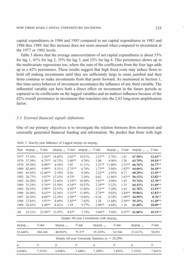
Table 3 shows that the average autocorrelation of net capital expenditures is about 53%for lag 1, 41% for lag 2, 35% for lag 3, and 32% for lag 4. This persistence shows up inthe multivariate regressions too, where the sum of the coefficients from the four lags addsup to a 62% persistence. These results suggest that high fixed costs may induce firms tohold off making investments until they are sufficiently large to seem justified and thenfirms continue to make investments from that point forward. As mentioned in Section 1,this time-series behavior of investment accentuates the influence of any third variable. Theinfluential variable can have both a direct effect on investment in the future periods ascaptured in its coefficients on the lagged variables and an indirect influence because of the62% overall persistence in investment that translates into the 2.63 long-term amplificationfactor.

3.3. External financial signals definitions

One of our primary objectives is to investigate the relation between firm investment andexternally generated financial funding and information. We predict that firms with high

Table 3. Year-by-year Influence of Lagged ntcpxp on ntcpxp0

Year ntcpxp21 T-stat ntcpxp22 T-stat ntcpxp23 T-stat ntcpxp24 T-stat ntcpxp21:24 T-stat

1977 37.16% 5.36** 14.05% 3.02** 10.51% 2.51** 5.78% 1.41 67.50% 12.42**1978 37.39% 6.75** 16.75% 3.40** 4.76% 1.00 4.90% 1.58 63.79% 10.54**1979 39.30% 8.40** 4.54% 1.05 11.11% 3.21** 11.80% 3.21** 66.76% 16.77**1980 42.66% 9.49** 9.31% 2.75** 6.74% 1.73** 5.88% 1.82** 64.60% 16.10**1981 45.85% 12.60** 2.19% 0.56 9.30% 2.22** 2.95% 0.77 60.29% 11.55**1982 24.77% 5.07** 17.33% 4.33* 2.36% 0.62 11.66% 3.41** 56.12% 12.82**1983 26.20% 6.20** 11.66% 3.18** 10.98% 3.07** 4.90% 1.43 53.74% 12.70**1984 33.24% 5.76** 15.59% 4.54** 10.37% 2.29** 5.22% 1.33 64.43% 11.69**1985 20.35% 3.99** 22.57% 4.58** 11.66% 2.33** 7.20% 1.63 61.78% 12.53**1986 26.48% 6.63** 12.36% 3.31** 11.99% 2.74** 9.03% 2.44** 59.86% 12.83**1987 26.56% 6.09** 12.54% 2.20** 20.86% 20.16 6.74% 1.98** 44.99% 8.76**1988 27.85% 5.97** 8.69% 2.42** 7.02% 1.28 11.68% 2.58** 55.25% 11.20**1989 38.42% 6.40** 8.61% 1.54 9.77% 2.40** 4.88% 1.16 61.68% 10.09**

All 33.21% 22.50** 12.97% 9.87* 7.74% 5.60** 7.94% 6.97** 61.86% 45.33**

Simple All-year Correlations with ntcpxp0

ntcpxp21 T-stat ntcpxp22 T-stat ntcpxp23 T-stat ntcpxp24 T-stat

52.646% 104.164 40.892% 75.377 35.339% 63.546 31.612% 56.051

Simple All-year Univariate Statistics (n 5 28,299)

µ s µ s µ s µ s

6.694% 7.353% 6.896% 7.440% 7.109% 7.493% 7.353% 7.841%



lagged equity financing and firm-specific returns will increase their investments.10 Wemeasure equity financing activity (ntissu) as new equity issuing activity (108) net ofequity repurchasing activity (115):

ntissu@t# 5 ~108@t# 2 115@t#!/Sz@t#.

Table 2 shows that net issuing activity is an average 0.9% of firms’ assets, has a cross-sectional standard deviation of 7.6%, and has a persistence of about 30%. Our measure ofthe firms’ stock returns, return, is the continuously compounded annual firm return fromCRSP aligned with the company’s fiscal year end.11 Table 2 shows that the average stockreturn in our sample is approximately 14%, with a cross-sectional standard deviation of37%.

3.4. Internal accounting information

We propose a number of proxies for the internal accounting information related to theinvestment decisions, income, dividends, changes in cash and short-term securities,changes in inventory, and depreciation. The first measure is net income (incom) measuredas net income before extraordinary items (18):

incom@t# 5 18@t#/Sz@t#.

A positive relation between net income and investment may be the result of two alternativemechanisms. First, large net income may indicate economic rents that have been and willbe earned by the firm. These opportunities may induce the firm to expand through invest-ment to capture as much of this rent as possible. Second, firm profitability is generally thesingle most important source of internal funds. Firms with substantial net income willultimately receive substantial inflows of cash through collection of accounts receivables.12

According to the free cash flow hypothesis, managers may choose to expand operationsbecause their incentives are not aligned with firm value maximization. Under either theeconomic rent seeking explanation or the free cash flow hypothesis, we predict that netincome will be positively related to investment. Table 2 shows that firms earn an averageof about 3.9% of their assets, with a cross-sectional standard deviation of 11.1%.

Our second internal information measure is dividends on common stock (21[t]):

divid@t# 5 21@t#/Sz@t#.

We investigate this variable to determine whether dividends are a complement or a sub-stitute for investment. An observed positive (negative) relation between dividends andinvestment would indicate a complementary (substitutive) role. Firms with high levels ofinternally generated cash may undertake both dividends and investment due to the abun-dance of relatively low cost internally generated capital. Alternatively, firms facing limited



investment opportunities may substitute dividends for investment. According to Table 2,firms in our sample paid about 1.7% of their assets in dividends, with a cross-sectionalstandard deviation of 6.6. About 2/3 of the firm-years in our sample paid cash dividends.

Our third internal information variable is the change in the balance of cash and cashequivalents (Dcash):

Dcash@t# 5 ~1@t# 2 1@t 2 1#!/Sz@t#.

Because investment requires liquidity, managers anticipating investments may rationallyincrease cash balances to reduce the transactions costs involved in the exchange. Ifchanges in cash and short-term securities holdings explain increases in investments, wewould favor hypotheses that argue managers either build slack to finance investments oruse free cash for investment. Table 2 shows changes in cash holdings are on average apositive 0.7% of assets.

Changes in total inventories, which is 1.1% of assets on average according to Table 2,is our fourth variable:

Dinvnt@t# 5 ~3@t# 2 3@t 2 1#!/Sz@t#.

Inventory changes can be inversely related to investment if firms respond to unusualincreases in real demand (as evidenced by a decline in inventories) by increasing invest-ment. Alternatively, managers could draw down inventories in anticipation of reduced realdemand and a decrease in required production capacity, which would lead to a positiverelation between inventory changes and investment.

Our fifth internal information variable is depreciation which is equivalent to the dif-ference between operating cash flow (opercf) and net income (incom) after controlling forchanges in working capital variables:

deprec@t# 5 opercf@t# 2 18@t#.

In our definition of investment, we note that we have difficulties adjusting for “economic”depreciation. Although including “accounting” depreciation as an independent variablemight allow us to control for some of the relationship between economic depreciation andinvestment, it is a somewhat limited proxy because accounting depreciation is computedfrom historical cost in a purely mechanical fashion (e.g., with the straight-line methoddepreciation equals historical cost/expected useful life). Thus, depreciation may proxysimply for past investment. A second reason to include depreciation is to allow the readerto compute the influence of operating cash flow, which is the sum of net income, depre-ciation, and working capital changes. Table 2 shows that firms depreciated an average of4.3% of their assets with a standard deviation of 13.3% and a persistence of about 21.5%.

In summary, these internal variables should cover the major components described infirms’ accounting reports. Furthermore, familiar concepts, such as operating cash flow,can be obtained from linear combinations of these measures.



3.5. Income tax definition

Finally, we measure the amount of taxes a firm pays (tax):

tax@t# 5 ~16@t# 2 50@t#!/Sz@t#

which is total income taxes (16[t]) net of deferred income taxes (50[t]). On average, firmspaid only 3.5% of their assets in taxes, with a typical cross-sectional standard deviation of4.3%. 20% of firms in our sample paid no taxes at all. Furthermore, income tax paymentswere persistent, displaying a typical 74% first order autocorrelation. Because we areinterested in correlations between taxes and investment in specific years, Figure 2 plots theyear-by-year cross-sectional average and standard deviation for taxes. The figure showsthat income taxes have been declining since 1977, reaching a low point in 1983. However,there is virtually no evidence that the firms in our sample faced significantly higher taxburdens when the investment tax credit and accelerated depreciation schedules wereabolished in 1986. Our firms were apparently either failing to take advantage of these taxadvantages before their repeal, or they were successful in substituting other tax reductionmethods after 1986.

3.6. Other variables

We include five different control variables all lagged over four periods to “hold everythingelse constant.” In particular, we include the following size-related variables: sales, changein sales, percentage change in assets, CPI-adjusted assets, and CPI-adjusted assetssquared. We also include 18 dummy variables for the 19 industry classifications describedin Table 12. Finally, we include the continuously compounded market return, the return ona treasury bill and the return on a long-term government bonds to replace traditional yeardummies for the regressions pooled across all years.

4. Methodology

Our regressions are specified as OLS vector autoregressions with White heteroscedasticity-adjusted standard errors. We estimate the influence of our included variables for lags fromone to four years and believe this approach captures most of the direct influence of ourvariables because the coefficients decrease steadily to the fourth lag. We do not use aninformation criteria to choose our lag length because this approach pre-tests the data set.Further, we include the lagged values of the dependent variable, net capital expenditures,to capture indirect effects and permit longer-lagged influences to enter our regressions.


Kluwer Journal@ats-ss11/data11/kluwer/journals/requ/v9n3art1 COMPOSED: 09/02/97 9:59 am. PG.POS. 12 SESSION: 15

We run the following regression for all firms for each of the 13 years from1977–1989:13

ntcpxpt 5 b1ntcpxpt21 1 b2ntcpxpt22 1 b3ntcpxpt23 1 b4ntcpxpt24

b5ntissut21 1 b6ntissut22 1 b7ntissut23 1 b8ntissut24

b9returnt21 1 b10returnt22 1 b11returnt23 1 b12returnt24

b13incomt21 1 b14incomt22 1 b15incomt23 1 b16incomt24

b17dividt21 1 b18dividt22 1 b19dividt23 1 b20dividt24

b21Dcasht21 1 b22Dcasht22 1 b23Dcasht23 1 b24Dcasht24

b25Dinvntt21 1 b26Dinvntt22 1 b27Dinvntt23 1 b28Dinvntt24

b29deprect21 1 b30deprect22 1 b31deprect23 1 b32deprect24

b33taxt21 1 b34taxt22 1 b35taxt23 1 b36taxt24 1 b37…76Control 1 «t

To allow the reader to easily gauge the overall determinants of investment, we group theresults of the 13 individual year regressions into Tables 3 through 11, with each tabledisplaying the influence of one particular variable. We also run and display “All” regres-sion for the observations pooled across firms and years. We do not display the coefficientson the control variables. Each table also presents the overall simple correlations of eachvariable with net capital expenditures in year 0. If the partial correlation represented in theregression coefficient shows significance in one direction and the simple correlationshows significance in the opposite direction, the measured effect may be difficult tointerpret given the multicollinearity in the accounting variables used. The mean and thestandard deviation of each variable are also presented to allow the reader to compute theeconomic significance of the individual variables by multiplying the standard deviationsby an estimated coefficient.

The reader must be warned that our cross-sectional and time-series vector autoregres-sions have unusual interpretations. In the cross-sectional autoregressions, the persistenceof variables as measured by their autocorrelation and their cross-sectional standard de-viation are very different. For example, we may describe the influence of a one standarddeviation higher variable X leading to a Y% increase in net capital expenditures. However,variable X may have 90% persistence; thus, individual firms may never experience a onecross-sectional standard deviation change in the variable across time. Furthermore, if avariable is autocorrelated, an effect on only lag 1, but not lags 2–4, may persist becausevariable X’s deviation from the mean is likely to continue. Including various lags of avariable theoretically allows us to disentangle the temporal influence, but variables withhigh multicollinearity may pick up each other’s significance in small samples. Thus, forcorrelated variables (e.g., dividends and net income), the reader may want to consider onlythe overall sum of coefficients on various lags.14


Kluwer Journal@ats-ss11/data11/kluwer/journals/requ/v9n3art1 COMPOSED: 09/02/97 10:00 am. PG.POS. 13 SESSION: 15

5. Results

5.1. Lagged net capital expenditures

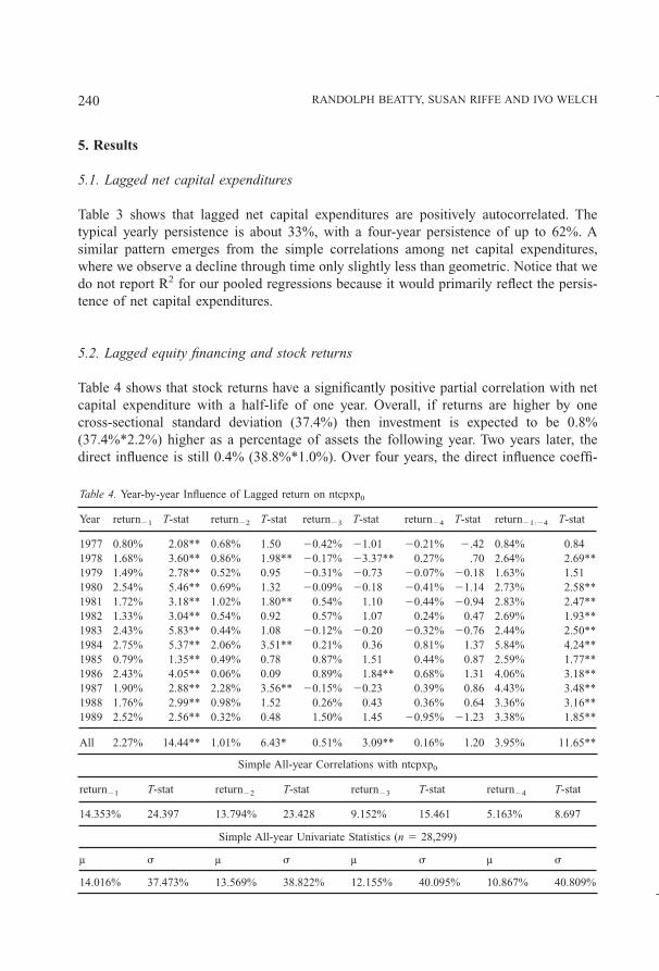
Table 3 shows that lagged net capital expenditures are positively autocorrelated. Thetypical yearly persistence is about 33%, with a four-year persistence of up to 62%. Asimilar pattern emerges from the simple correlations among net capital expenditures,where we observe a decline through time only slightly less than geometric. Notice that wedo not report R2 for our pooled regressions because it would primarily reflect the persis-tence of net capital expenditures.

5.2. Lagged equity financing and stock returns

Table 4 shows that stock returns have a significantly positive partial correlation with netcapital expenditure with a half-life of one year. Overall, if returns are higher by onecross-sectional standard deviation (37.4%) then investment is expected to be 0.8%(37.4%*2.2%) higher as a percentage of assets the following year. Two years later, thedirect influence is still 0.4% (38.8%*1.0%). Over four years, the direct influence coeffi-

Table 4. Year-by-year Influence of Lagged return on ntcpxp0

Year return21 T-stat return22 T-stat return23 T-stat return24 T-stat return21:24 T-stat

1977 0.80% 2.08** 0.68% 1.50 20.42% 21.01 20.21% 2.42 0.84% 0.841978 1.68% 3.60** 0.86% 1.98** 20.17% 23.37** 0.27% .70 2.64% 2.69**1979 1.49% 2.78** 0.52% 0.95 20.31% 20.73 20.07% 20.18 1.63% 1.511980 2.54% 5.46** 0.69% 1.32 20.09% 20.18 20.41% 21.14 2.73% 2.58**1981 1.72% 3.18** 1.02% 1.80** 0.54% 1.10 20.44% 20.94 2.83% 2.47**1982 1.33% 3.04** 0.54% 0.92 0.57% 1.07 0.24% 0.47 2.69% 1.93**1983 2.43% 5.83** 0.44% 1.08 20.12% 20.20 20.32% 20.76 2.44% 2.50**1984 2.75% 5.37** 2.06% 3.51** 0.21% 0.36 0.81% 1.37 5.84% 4.24**1985 0.79% 1.35** 0.49% 0.78 0.87% 1.51 0.44% 0.87 2.59% 1.77**1986 2.43% 4.05** 0.06% 0.09 0.89% 1.84** 0.68% 1.31 4.06% 3.18**1987 1.90% 2.88** 2.28% 3.56** 20.15% 20.23 0.39% 0.86 4.43% 3.48**1988 1.76% 2.99** 0.98% 1.52 0.26% 0.43 0.36% 0.64 3.36% 3.16**1989 2.52% 2.56** 0.32% 0.48 1.50% 1.45 20.95% 21.23 3.38% 1.85**

All 2.27% 14.44** 1.01% 6.43* 0.51% 3.09** 0.16% 1.20 3.95% 11.65**


return21 T-stat return22 T-stat return23 T-stat return24 T-stat

14.353% 24.397 13.794% 23.428 9.152% 15.461 5.163% 8.697


µ s µ s µ s µ s

14.016% 37.473% 13.569% 38.822% 12.155% 40.095% 10.867% 40.809%



cients add up to 4.0%, indicating the direct influence of a 37% increase in stock returnsto be a 1.5% increase in investment. When this influence is multiplied by the long-terminvestment persistence factor of 2.63, the total influence equals 4%. Thus, we believe thatstock performance acts as an important economic determinant of subsequent, cross-sectional investment decisions. Returns can also absorb some of the explanatory poweravailable in the accounting variables, and vice-versa. For example, managers may investbecause of their superior stock market performance, which in turn may be determined bythe outstanding past financial performance of the company.

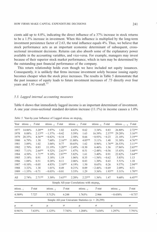
This return relationship holds even though we have included net equity issuances.Consequently, it is unlikely that firms increase investment solely because issuing equitybecomes cheaper when the stock price increases. The results in Table 5 demonstrate thatthe past issuance of equity leads to future investment increases of .73 directly over fouryears and 1.93 overall.15

5.3. Lagged internal accounting measures

Table 6 shows that immediately lagged income is an important determinant of investment.A one year cross-sectional standard deviation increase (11.1%) in income causes a 1.0%

Table 5. Year-by-year Influence of Lagged ntissu on ntcpxp0

Year ntissu21 T-stat ntissu22 T-stat ntissu23 T-stat ntissu24 T-stat ntissu21:24 T-stat

1977 14.86% 3.20** 3.97% 1.02 4.63% 0.62 3.34% 0.83 26.80% 2.72**1978 8.88% 2.13** 21.57% 20.42 5.59% 1.63 16.39% 2.37** 29.28% 3.16**1979 20.35% 4.36** 20.82% 20.18 2.58% 0.66 20.93% 20.23 21.18% 3.19**1980 6.79% 1.30 7.60% 2.16** 11.80% 4.05** 5.11% 1.48 31.30% 4.76**1981 3.89% 1.02 3.04% 0.77 10.65% 1.62 8.96% 1.76** 26.53% 3.11**1982 2.70% 0.83 11.19% 3.20** 22.49% 20.30 6.46% 1.36 17.86% 2.65**1983 7.11% 2.64** 9.32% 2.61** 1.47% 0.51 22.48% 20.56 15.43% 3.44**1984 4.50% 1.71** 9.10% 2.87** 5.82% 1.61 3.40% 0.91 22.82% 3.64**1985 3.18% 0.91 3.18% 1.19 1.06% 0.35 21.56% 20.62 5.85% 1.131986 1.88% 0.51 0.28% 0.11 2.06% 0.83 1.30% 0.43 5.51% 1.101987 20.10% 20.05 4.83% 2.10** 4.19% 1.50 0.65% 0.26 9.57% 2.94**1988 3.32% 1.38 1.01% 0.49 0.21% 0.09 22.46% 20.69 2.09% 0.511989 21.35% 20.71 20.03% 20.01 3.33% 1.29 3.36% 1.93** 5.31% 1.70**

All 2.74% 2.71** 3.30% 3.63** 2.20% 2.23** 1.36% 1.47 9.60% 6.45**


ntissu21 T-stat ntissu22 T-stat ntissu23 T-stat ntissu24 T-stat

4.589% 7.727 3.712% 6.248 1.763% 2.966 20.438% 20.737


µ s µ s µ s µ s

0.941% 7.635% 1.125% 7.743% 1.204% 7.634% 1.297% 7.791%



difference in investment the following year. This amount is roughly equivalent to theimmediate increase in investment due to an unusually high stock return. However, unlikethe influence of stock returns (a non-persistent variable), the influence of income (a verypersistent variable) is concentrated in the immediately preceding year. Furthermore, be-cause stock returns are more likely to significantly shift from year to year, stock returnswill have a greater long-term effect as well.

In contrast, Table 7 shows that dividends act as a substitute for future investment overthe next 2 years. The economic significance of dividends as a determinant of net capitalexpenditures is considerably lower than that of income. A firm with a one-standarddeviation higher dividend payout rate (6.6%) suggests an 0.3% higher investment rate thefollowing year and the year after.

As Table 8 shows, changes in cash and short-term holdings can explain some invest-ment, too. Investment changes are particularly powerful with a two year lag, with anoverall coefficient of 1.6%. The overall 4-year direct impact of a one standard deviationhigher cash increase (7.7%) is an 0.3% higher investment rate.

In contrast, Table 9 shows that changes in inventory were largely unimportant. Thus, wedo not have good evidence that real demand changes have a strong immediate impact oninvestment. The exception is in 1984 and 1985 years when there is an unexplainablepositively correlation between inventory and investment changes.

Table 6. Year-by-year Influence of Lagged incom on ntcpxp0

Year incom21 T-stat incom22 T-stat incom23 T-stat incom24 T-stat incom21:24 T-stat

1977 14.02% 2.28** 6.72% 1.11 8.50% 1.59 0.19% 0.03 29.43% 4.24**1978 19.37% 2.52** 20.65% 20.12 6.00% 1.22 8.23% 1.62 32.94% 3.57**1979 18.32% 4.00** 7.63% 1.91** 26.82% 21.55 7.37% 2.09** 26.50% 4.60**1980 8.28% 1.73** 13.92% 2.79** 3.61% 0.79 20.64% 20.16 25.17% 4.56**1981 19.17% 3.54** 1.63% 0.30 28.11% 21.21 9.44% 2.08** 22.13% 3.46**1982 13.88% 2.67** 5.43% 1.21 4.01% 0.92 2.54% 0.51 25.87% 3.98**1983 10.20% 2.50** 3.89% 0.77 6.99% 1.25 3.32% 0.84 24.40% 3.35**1984 10.47% 2.07** 9.00% 1.94** 10.53% 1.34 211.45% 21.80** 18.55% 2.05**1985 16.03% 4.65** 213.22% 22.18** 6.37% 1.44 22.99% 20.73 6.20% 0.981986 6.06% 1.82** 4.30% 1.23 22.17% 20.46 0.32% 0.06 8.52% 1.72**1987 4.84% 1.74** 7.70% 2.46** 2.21% 0.52 0.29% 0.06 15.04% 3.36**1988 6.89% 2.73** 0.46% 0.16 2.54% 0.88 2.15% 0.68 12.04% 3.01**1989 6.73% 1.57 1.59% 0.42 21.33% 20.42 6.86% 2.01** 13.86% 3.25**

All 8.84% 7.08** 2.24% 1.80* 0.87% 0.72 2.52% 2.05** 14.47% 9.04**


incom21 T-stat incom22 T-stat incom23 T-stat incom24 T-stat

17.441% 29.796 12.984% 22.028 8.548% 14.432 6.168% 10.395


µ s µ s µ s µ s

3.920% 11.100% 4.412% 10.650% 4.776% 10.483% 5.216% 10.288%



Finally, Table 10 finds that depreciation, another component in the calculation of cashflows, is positively correlated with future investment. Since operating cash flows arepredominantly net income and depreciation, the positive relation of both depreciation andnet income with investment suggests that operating cash flows are strongly related to newinvestment. Thus, firms experiencing increased cash inflow are more likely to undertakenew investment.

5.4. Income taxes

Until the Tax Reform Act of 1986, the tax code offered two provisions that were likely tohave significant influence on investments during the sample period, accelerated deprecia-tion schedules and the investment tax credit. From 1981 through 1986, the tax codesignificantly accelerated depreciation schedules. Also, the investment tax credit was avail-able from 1971–1986. Table 11 indicates a strong relation between investments and taxesfor both 1985 and 1986 prior to the repeal of both the accelerated depreciation schedulesand the investment tax credit. One can show using a reasonable set of assumptions that thet-statistics of 2.32 and 1.97 in these two years are significantly different from the otheryears. The average t-statistic for the years excluding 1985 and 1986 have a mean of 20.96

Table 7. Year-by-year Influence of Lagged divid on ntcpxp0

Year divid21 T-stat divid22 T-stat divid23 T-stat divid24 T-stat divid21:24 T-stat

1977 27.55% 20.44 212.07% 20.73 2.19% 0.16 212.73% 20.87 230.16% 24.40**1978 217.72% 20.77 26.26% 20.16 5.99% 0.28 215.37% 21.17 233.36% 23.61**1979 236.28% 20.93 2.48% 0.06 3.93% 0.14 4.69% 0.24 225.18% 24.18**1980 24.40% 21.04 2.06% 0.18 26.39% 20.23 214.54% 20.60 223.25% 24.04**1981 216.21% 21.62 0.47% 0.05 23.67% 0.97 230.47% 21.59 222.53% 23.46**1982 217.29% 21.85** 2.96% 0.30 23.99% 20.28 211.10% 20.78 229.42% 24.48**1983 0.22% 0.04 213.67% 22.72** 23.86% 20.63 29.03% 21.83** 226.33% 23.60**1984 27.18% 21.52 29.34% 20.88 217.66% 22.58** 14.43% 1.52 219.76% 22.20**1985 0.22% 0.08 21.38% 20.43 23.15% 20.50 23.31% 20.46 27.61% 21.171986 28.56% 23.00** 21.54% 20.45 20.21% 0.06 0.11% 0.02 29.77% 21.96**1987 2.06% 0.42 28.92% 22.00** 24.29% 21.09 21.59% 20.49 212.74% 22.55**1988 27.23% 22.54** 25.82% 21.48 1.34% 0.37 21.58% 0.60 213.29% 23.07**1989 22.65% 21.83** 28.36% 21.95** 1.22% 0.20 25.67% 21.04 215.46% 23.24**

All 24.59% 23.39** 24.72% 22.54** 22.94% 21.44 22.47% 21.35 214.71% 28.97**


divid21 T-stat divid2 T-stat divid23 T-stat divid24 T-stat

21.965% 23.306 22.317% 23.899 22.377% 24.000 22.602% 24.378


µ s µ s µ s µ s

1.722% 6.585% 1.698% 6.442% 1.684% 6.487% 1.681% 6.656%



with a standard deviation of 0.91. Under the admittedly mistaken assumption that thet-statistics are normally distributed and independent, the probability of observing a 2.32or a 1.97 t-statistic is far below the 1% significance level. This can be seen graphically inFigure 3. There was also a significant negative relationship between investment and taxesin 1977 and 1978. The Tax Reform Act of 1976 extended the investment tax credit through1980, and the Revenue Act of 1978 permanently extended the 10% tax credit. Thus, thesignificant negative coefficients on the tax variables in 1977 and 1978 are consistent withthe interpretation that changes in the tax code caused firms to believe they could delayinvestment until future periods and still take advantage of the tax credit.

5.5. Industry dummy coefficients

Finally, Table 12 describes the industry dummy definitions used in all regressions and thesimple and partial correlations with net capital expenditures. Although these coefficientsmust be interpreted relative to the service industry which is captured by the overallintercept, we find that firms in real-estate, financial services and insurance invested lessthan suggested by our model. Firms in both the oil and gas industry and the services sectorinvested more than expected. Table 13 contains the number of observations in these

Table 8. Year-by-year Influence of Lagged Dcash on ntcpxp0

Year Dcash21 T-stat Dcash22 T-stat Dcash23 T-stat Dcash24 T-stat Dcash21:24 T-stat

1977 3.24% 1.17 7.08% 2.83** 2.72% 0.99 4.61% 1.42 17.65% 3.07**1978 5.93% 1.74** 9.71% 3.46** 0.28% 0.10 20.19% 20.06 15.73% 2.16**1979 2.56% 0.70 8.61% 2.99** 6.62% 2.27** 5.29% 2.34** 23.08% 3.26**1980 7.87% 2.82** 4.97% 1.94** 7.90% 3.11** 3.24% 1.39 23.97% 4.27**1981 1.50% 0.53 2.44% 0.90 22.28% 20.69 0.18% 0.07 1.84% 0.261982 8.16% 2.52** 4.31% 1.37 20.04% 20.01 10.44% 3.48** 22.87% 2.88**1983 20.58% 20.20 4.16% 1.43 20.52% 20.20 3.11% 1.08 6.17% 1.071984 21.39% 20.49 3.52% 1.18 5.97% 1.87** 8.65% 2.65** 16.75% 2.84**1985 0.76% 0.35 2.32% 0.87 3.06% 1.06 20.09% 20.03 6.06% 0.911986 0.67% 0.25 3.89% 1.46 1.92% 0.81 2.73% 0.90 9.21% 1.311987 1.31% 0.48 23.21% 20.90 24.32% 21.47 5.70% 1.93** 20.52% 20.071988 3.63% 1.36 2.01% 0.97 21.82% 20.82 23.03% 21.41 0.80% 0.171989 25.96% 21.03 23.78% 21.13 22.98% 20.56 24.29% 21.49 217.01% 21.12

All 0.84% 0.85 1.64% 1.92** 0.63% 0.68 1.24% 1.48 4.35% 1.71**


Dcash21 T-stat Dcash22 T-stat Dcash23 T-stat Dcash24 T-stat

3.395% 5.714 4.524% 7.618 1.537% 2.586 0.263% 0.443


µ s µ s µ s µ s

0.701% 7.740% 0.907% 7.759% 0.958% 7.715% 0.814% 8.055%



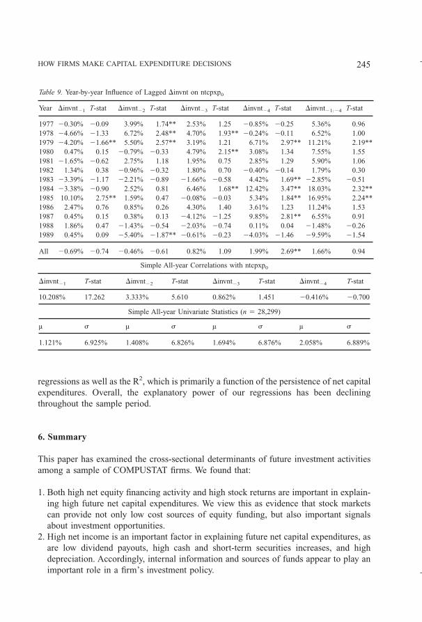
regressions as well as the R2, which is primarily a function of the persistence of net capitalexpenditures. Overall, the explanatory power of our regressions has been decliningthroughout the sample period.

6. Summary

This paper has examined the cross-sectional determinants of future investment activitiesamong a sample of COMPUSTAT firms. We found that:

1. Both high net equity financing activity and high stock returns are important in explain-ing high future net capital expenditures. We view this as evidence that stock marketscan provide not only low cost sources of equity funding, but also important signalsabout investment opportunities.

2. High net income is an important factor in explaining future net capital expenditures, asare low dividend payouts, high cash and short-term securities increases, and highdepreciation. Accordingly, internal information and sources of funds appear to play animportant role in a firm’s investment policy.

Table 9. Year-by-year Influence of Lagged Dinvnt on ntcpxp0

Year Dinvnt21 T-stat Dinvnt22 T-stat Dinvnt23 T-stat Dinvnt24 T-stat Dinvnt21:24 T-stat

1977 20.30% 20.09 3.99% 1.74** 2.53% 1.25 20.85% 20.25 5.36% 0.961978 24.66% 21.33 6.72% 2.48** 4.70% 1.93** 20.24% 20.11 6.52% 1.001979 24.20% 21.66** 5.50% 2.57** 3.19% 1.21 6.71% 2.97** 11.21% 2.19**1980 0.47% 0.15 20.79% 20.33 4.79% 2.15** 3.08% 1.34 7.55% 1.551981 21.65% 20.62 2.75% 1.18 1.95% 0.75 2.85% 1.29 5.90% 1.061982 1.34% 0.38 20.96% 20.32 1.80% 0.70 20.40% 20.14 1.79% 0.301983 23.39% 21.17 22.21% 20.89 21.66% 20.58 4.42% 1.69** 22.85% 20.511984 23.38% 20.90 2.52% 0.81 6.46% 1.68** 12.42% 3.47** 18.03% 2.32**1985 10.10% 2.75** 1.59% 0.47 20.08% 20.03 5.34% 1.84** 16.95% 2.24**1986 2.47% 0.76 0.85% 0.26 4.30% 1.40 3.61% 1.23 11.24% 1.531987 0.45% 0.15 0.38% 0.13 24.12% 21.25 9.85% 2.81** 6.55% 0.911988 1.86% 0.47 21.43% 20.54 22.03% 20.74 0.11% 0.04 21.48% 20.261989 0.45% 0.09 25.40% 21.87** 20.61% 20.23 24.03% 21.46 29.59% 21.54

All 20.69% 20.74 20.46% 20.61 0.82% 1.09 1.99% 2.69** 1.66% 0.94


Dinvnt21 T-stat Dinvnt22 T-stat Dinvnt23 T-stat Dinvnt24 T-stat

10.208% 17.262 3.333% 5.610 0.862% 1.451 20.416% 20.700


µ s µ s µ s µ s

1.121% 6.925% 1.408% 6.826% 1.694% 6.876% 2.058% 6.889%



3. Changes in inventories are not significantly related to future net capital expenditures.This suggests that short-term fluctuations in real demand are dominated by the influ-ence of other variables.

4. Prior to 1985, firms with high income tax payments tended to invest less than equivalentfirms. However, the Tax Reform Act of 1986 significantly altered firms’ investmentbehavior. Firms with high income taxes rushed to take advantage of the investment taxcredit and the accelerated depreciation schedules in 1985 and 1986, just as they were inthe process of being eliminated. We view this as evidence that tax code changes in the1980’s significantly influenced firms’ investment policies. This finding provides im-portant evidence that the 1986 Tax Reform Act had a real effect on the investmentbehavior of firms.

5. Firms in real-estate, financial services and insurance prominently invested less thansuggested by our model. Firms in both the oil and gas industry and the services sectorinvested more than predicted.

While this paper provides the important insights described above, we want to recognizethe limitations of the analysis. First, in an empirical exercise such as ours, the variablesincluded reflect our own “priors” of what constructs are most important. Second, whileour empirical methodology minimizes the risk of bias from correlated omitted variables,

Table 10. Year-by-year Influence of Lagged deprec on ntcpxp0

Year deprec21 T-stat deprec22 T-stat deprec23 T-stat deprec24 T-stat deprec21:24 T-stat

1977 4.04% 2.06** 4.21% 2.07** 3.77% 1.96** 4.44% 2.07** 16.46% 4.23**1978 7.67% 2.40** 4.60% 1.63 3.24% 1.43 2.88% 1.37 18.39% 3.74**1979 6.83% 2.62** 1.74% 0.98 1.46% 20.79 1.98% 1.04 9.09% 2.58**1980 1.41% 0.47 4.41% 2.10** 3.02% 1.69** 2.09% 1.05 10.93% 2.90**1981 1.41% 0.63 3.16% 1.08 4.12% 1.65** 6.47% 2.23** 15.16% 3.41**1982 2.18% 0.90 4.48% 2.06** 0.89% 0.38 6.46% 2.21** 14.01% 3.08**1983 0.68% 0.35 3.19% 1.35 1.09% 0.64 21.41% 20.65 3.55% 1.001984 20.99% 20.32 2.70% 1.33 5.67% 1.97** 6.40% 2.59** 13.77% 2.86**1985 11.11% 3.80** 22.33% 20.78 0.38% 0.21 21.41% 20.64 7.74% 1.65**1986 22.52% 21.69** 1.15% 0.70 2.78% 1.40 1.90% 1.17 3.32% 1.211987 1.41% 1.07 5.41% 3.31** 0.87% 0.44 21.41% 20.47 6.28% 1.81**1988 21.50% 20.84 21.62% 20.75 1.90% 0.87 1.16% 0.74 20.06% 20.021989 3.26% 1.11 20.83% 20.48 2.74% 1.88** 20.81% 20.35 4.37% 1.27

All 1.43% 2.27** 1.11% 1.78* 1.49% 2.81** 0.91% 1.36 4.95% 4.38**


deprec21 T-stat deprec22 T-stat deprec23 T-stat deprec24 T-stat

92.080% 3.500 95.716% 9.631 98.802% 14.864 99.985% 16.880


µ s µ s µ s µ s

4.223% 13.296% 3.590% 11.849% 3.156% 11.453% 2.575% 11.028%



Table 11. Year-by-year Influence of Lagged tax on ntcpxp0

Year tax21 T-stat tax22 T-stat tax23 T-stat tax24 T-stat tax21:24 T-stat

1977 0.91% 0.02 24.81% 20.54 25.41% 20.74 21.13% 20.16 211.16% 22.50**1978 23.26% 20.38 8.01% 1.14 28.81% 20.99 26.89% 21.15 210.95% 22.21**1979 29.47% 20.98 6.53% 0.78 11.74% 1.68** 212.85% 22.27** 24.04% 20.951980 9.69% 1.59 29.62% 21.26 20.47% 20.06 0.44% 0.07 0.04% 0.011981 6.32% 0.98 25.62% 20.79 5.96% 0.71 28.31% 21.33 21.66% 20.361982 1.04% 0.15 3.12% 0.42 211.04% 21.66** 0.98% 0.16 25.89% 21.381983 20.33% 20.06 0.38% 0.05 25.54% 20.71 22.73% 20.44 28.22% 21.571984 0.82% 0.08 25.03% 20.66 28.93% 20.92 10.52% 1.19 22.62% 20.411985 1.08% 0.17 21.39% 2.45** 210.02% 21.38 0.32% 0.05 12.77% 2.32**1986 3.02% 0.45 5.20% 0.71 21.03% 20.12 3.77% 0.56 10.96% 1.97**1987 1.32% 0.22 29.27% 21.46 4.73% 0.65 23.89% 20.52 27.11% 21.301988 20.68% 20.13 4.46% 0.76 5.25% 0.79 28.82% 21.49 0.21% 0.041989 2.85% 0.33 5.24% 0.63 24.87% 20.75 22.60% 20.49 0.62% 0.09

All 2.84% 1.37 2.12% 0.98 20.61% 20.30 23.95% 22.20** 0.40% 0.28


tax21 T-stat tax22 T-stat tax23 T-stat tax24 T-stat

12.542% 21.266 11.499% 19.473 8.276% 13.970 5.308% 8.942


µ s µ s µ s µ s

3.481% 4.304% 3.667% 4.470% 3.825% 4.549% 4.036% 4.627%

Figure 3. Sum of Lagged Income Tax Coefficient T-Statistics Predicting Net Captial Expenditures - Yearby Year In years before 1985 and 1986, there is a weak evidence for a negative coefficient: the firms experi-encing the highest income tax burden (holding cash flow constant) increased thir capital expenditures less thanlow income tax firms. However, in 1985 and 986, the same firms increased their capital expenditures more thanother firms.



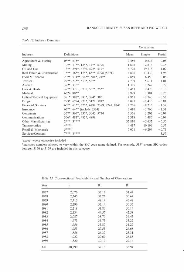
Table 12. Industry Dummies

Industry

Correlation

Definitions Mean Simple Partial

Agriculture & Fishing 0***, 515* 0.459 0.533 0.08Mining 10**, 11**, 12**, 14**, 6795 1.608 2.816 0.38Oil and Gas 13**, 291*, 6792, 492*, 517* 6.728 19.718 1.09Real Estate & Construction 15**, 16**, 17**, 65**, 6798 (5271) 4.806 213.430 21.96Food & Tobacco 20**, 514**, 54**, 581*, 21** 7.859 6.450 0.06Textiles 22**, 23**, 513*, 56** 4.739 25.611 21.01Aircraft 372*, 376* 1.385 21.247 2.79Cars & Boats 37**, 3751, 3730, 55**, 75** 0.463 2.470 20.10Medical 6324, 80** 0.929 1.384 20.25Optical/Medical Equipment 381*, 382*, 383*, 384*, 3851 4.961 22.740 20.53Drugs 283*, 6794, 873*, 5122, 5912 3.081 22.410 20.81Financial Services 60**, 61**, 62**, 6799, 7389, 8741, 8742 2.756 28.216 21.39Insurance 63**, 64** [include 6324] 0.410 22.760 21.51Computers 357*, 367*, 737*, 5045, 5734 6.566 3.202 20.04Communications 366*, 481*, 482*, 4899 2.318 1.486 20.04Other Manufacturing 2***, 3***† 32.810 25.652 20.50Transportation 4***† 4.417 10.196 0.57Retail & Wholesale 5***† 7.071 26.299 20.75Services/Constant 7***, 8***† — — 3.57

†except where otherwise included*indicates numbers allowed to vary within the SIC code range defined. For example, 515* means SIC codesbetween 5150 to 5159 are included in this category.

Table 13. Cross-sectional Predictability and Number of Observations

Year n R2 R̄2

1977 2,076 53.17 51.441978 2,245 52.27 50.641979 2,315 48.19 46.481980 2,296 52.14 50.551981 2,218 51.80 50.141982 2,134 44.57 42.581983 2,087 38.70 36.451984 1,973 35.73 33.221985 1,956 33.87 31.271986 1,953 27.53 24.681987 1,856 26.37 23.311988 1,922 29.69 26.881989 1,820 30.10 27.14

All 28,299 37.13 36.94



there is a possibility that multicollinearity may be affecting our analysis. Third, dealingwith endogeneity inherent in the chosen variables relating to investment is an intriguingand important issue that remains an open question for future research.

Acknowledgements

Ivo Welch wishes to thank the Olin Foundation and Michael Darby for support. We wouldalso like to thank Robert Hauswald and Dennis Logue for helpful comments.

Notes

1. This indirect influence is based on an amplification factor used commonly in the macro-economic literature,1/(1-coefficient on lagged variable). To illustrate the intuition, consider a dependent variable Y that followsa random walk (i.e., the coefficient on its own lagged variable is 1). Thus, if a third variable causes a 1%change in Y, this variable would cause a 1% change forever or a long-term effect of infinity. If Y is astationary variable (i.e., the coefficient on its own lagged variable is 0), the third variable would cause onlya one-time change of 1% or a long-term effect of 1%.

2. All financial statement variables are expressed as a percentage of assets. See Table 1 for the variabledefinitions. For example, if a $200M firm invested $25M in 1989, then 1989 investment is computed as12.5%.

3. For example, .2% is calculated as the 7.6% standard deviation times the 2.74% one year lag coefficient forthe pooled regression reported in Table 5. .73% is calculated as 7.6% times 9.6%, which is the sum of thefour lagged coefficients in the pooled regression.

4. The significance of stock returns does not diminish when lagged equity issuing activity is not included asa predictor.

5. Note that a positive correlation between investment and free cash flow (or related variables) is not incon-sistent with Modigliani-Miller. Firms with free cash flow may have better investment opportunities or mayincrease cash holdings in anticipation of a large investment.

6. See Williamson and Pijor [1990] for a detailed discussion of the tax code in the 1980’s.7. A number of other papers examine investment decisions cross-sectionally but do not focus on the influence

of financial markets. For example, Foresi and Mei (1991) find industry effects that can be interpreted ascascading behavior (see Bikhchandhani, Hirshleifer and Welch [1991]). Bar-Yosef, Callen and Livnat(1987) find that earnings are good predictors of investment, but they do not find evidence that investmentis a good predictor of earnings.

8. Unlike MSV, we do not find that when we use yearly data, the only variables showing significance inregressions predicting investment are industry intercepts.

9. We will use the casual notation “n[t]” to refer to data item n on the COMPUSTAT tapes. For example, 128[t]refers to capital expenditures, which is item 128 on the Compustat tapes in year t.

10. Our finding is consistent with the hypothesis that stock returns signal improved investment opportunities. Ofcourse, in some firms, increases in stock values might have been caused by increases in market power andcapacity reduction. On average, our evidence rejects this hypothesis.

11. Unlike most other variables, the return measure is not standardized for size because returns are standardizedby definition.

12. This assertion can be verified by noting that the difference between cash flow from operations and netincome is merely the difference in inventory, accounts receivable, accounts payable, and depreciation levels.The cash flow statement makes this point clear.

13. The 38 control variables (from b37 to b76) are the 4 lags of the 5 size variables plus the 18 industrydummies.



14. To make sure that our results are not driven by programming errors, we asked two different researchassistants to confirm the reported results.

15. We do not report the regression results when including contemporaneous equity issuances. Although ourresults remain the same with this approach, our regressions would no longer be purely predictive.

References

Barro, R. “The Stock Market and Investment,” The Review of Financial Studies, 3–1, 115–131 (1990).Bar-Yosef, S., J. L. Callen, and J. Livnat. “Autoregressive Modeling of Earnings-Investment Causality,” Journal

of Finance, 42, 11–28 (1987).Bikhchandhani, S., D. Hirshleifer, and I. Welch. “A Theory of Fads, Fashions, Customs and Cultural Change as

Informational Cascades,” The Journal of Political Economy, 100, 992–1026 (1991).Coase, R.H. “The Nature of the Firm,” Economica, 386–405 (1937).Chirinko, Robert S. “Business Fixed Investment Spending: Modeling Strategies, Empirical Results, and Policy

Implications.” Journal of Economic Literature, 31, 1875–1911 (1993).Copeland, T. and J. Weston. Financial Theory and Corporate Policy. Reading, Mass: Addison-Wesley, (1983).Foresi, S. and J. Mei. “Do Firms Keep Up with the Joneses?,” unpublished working paper, New York University

(1991).Fama, E. and K. French. “Permanent and Temporary Components of Stock Prices,” Journal of Political

Economy, 96, 246–273 (1988).Fazzari, Steven M., R. G. Hubbard and B. C. Petersen. “Financing Constrains Corporate Investment,” Brookings

Papers on Economic Activity, 1, 141–205 (1988).Financial Accounting Standards Board. Statement of Financial Accounting Concepts. Homewood, Illinois: Irwin

(1988).Jensen, M. C. “Agency Costs of Free Cash Flow, Corporate Finance and Takeovers,” American Economic

Review, May 1986, 76, 323–329 (1976).Jensen, M. C. and W. Meckling. “Theory of the Firm: Managerial Behavior, Agency Costs and Ownership

Structure,” Journal of Financial Economics, 3, 306–330 (1976).Modigliani, F. and M. H. Miller. “The Cost of Capital, Corporation Finance and the Theory of Investment,”

American Economic Review, 48, 261–297 (1958).Morck, R., A. Shleifer, and R. Vishny. “The Stock Market and Investment: Is the Market a Side-Show?”

Brookings Papers on Economic Activity with discussions by Matthew Shapiro and James Poterba, 2, 157–215(1990).

Myers, S. C. and N. S. Majluf. “Corporate Financing And Investment Decisions When Firms Have InformationThat Investors Do Not Have,” Journal of Financial Economics, v13(2), 187–221 (1984).

Tobin, J. “A General Equilibrium Approach to Monetary Theory,” Journal of Money, Credit and Banking, 1,15–29 (1969).

Williamson, D. and D. Pijor. “Income Tax Credits: The Investment Credit,” Tax Management, 191–5th, 69–74(1990).



how firms make capital expenditure decisions: · pdf filemany opportunities and insufﬁcient...

Documents