How Does Trade Evolve in the Aftermath of Financial Crises?

Abdul Abiad, Prachi Mishra, and Petia

Topalova

WP/11/3

© 2010 International Monetary Fund WP/1 / IMF Working Paper Research Department

How Does Trade Evolve in the Aftermath of Financial Crises?

Prepared by Abdul Abiad, Prachi Mishra, and Petia Topalova1

Authorized for Distribution by Andrew Berg and Petya Koeva Brooks 201

Abstract We analyze trade dynamics following past episodes of financial crises. Using an augmented gravity model and 179 crisis episodes from 1970-2009, we find that there is a sharp decline in a country’s imports in the year following a crisis—19 percent, on average—and this decline is persistent, with imports recovering to their gravity-predicted levels only after 10 years. In contrast, exports of the crisis country are not adversely affected, and they remain close to the predicted level in both the short and medium-term.

JEL Classification Numbers: F10, G01

Keywords: trade, financial crises

Author’s E-Mail Address: aabiad@imf.org; pmishra@imf.org, ptopalova@imf.org

This Working Paper should not be reported as representing the views of the IMF. The views expressed in this Working Paper are those of the author(s) and do not necessarily represent those of the IMF or IMF policy. Working Papers describe research in progress by the author(s) and are published to elicit comments and to further debate.

1 We are grateful to Andrew Berg, Olivier Blanchard, Don Davis, Petya Koeva Brooks, David Romer, Philippe Martin, Andrei Levchenko, and seminar participants at the World Bank, IMF, Hong Kong University of Science and Technology, Indira Gandhi Institute for Development Research, ICRIER, and the Delhi School of Economics for helpful comments. We thank Gavin Asdorian, Stephanie Denis, Lisa Kolovich, Andy Salazar and Yorbol Yakhshilikov for excellent research assistance. We thank Peter Pedroni for kindly providing the programs to perform panel unit root and cointegration tests

2

Contents Page

I. Introduction .......................................................................................................................4

II. Methodology .....................................................................................................................6

III. A First Look at the Data ....................................................................................................8

IV. Gravity Framework Results ..............................................................................................9 A. Main Findings ...............................................................................................................9 B. Robustness ..................................................................................................................13

V. Differences in Trade Dynamics Across Products, During Global Downturns, and Over Time ................................................................................................................................18 A. Do Postcrisis Trade Dynamics Vary Across Products? .............................................18 B. Are Postcrisis Trade Dynamics Different During Global Downturns? ......................20 C. Do Postcrisis Trade Dynamics Vary Over Time? ......................................................21

VI. Conclusions .....................................................................................................................22

VII. Tables Table 1. Sample Characteristics ......................................................................................24 Table 2. Imports and Exports Following Crises: Pooled Panel Gravity Estimates, 1970-2009 .......................................................................................................................25 Table 3. Tariff Equivalent Trade Costs ...........................................................................26 Table 4. Imports and Exports Following Crises: Robustness .........................................26 Table 5. Reverse Causality Issues ...................................................................................28 Table 6. Imports and Exports of Various Product Categories Following Crises ............30

VIII. Figures Figure 1. Growth Rate of World Real Imports ..............................................................32 Figure 2. Evolution of Imports in Crisis and Non-Crisis Countries ...............................33 Figure 3. Distribution of Crises across Time and Regions .............................................34 Figure 4. Evolution of Imports and Exports Following Crises: A First Look ................35 Figure 5. Evolution of Imports and Exports Following Crises: Gravity Model .............36 Figure 6a. Evolution of Exchange Rates Following Crises ............................................37 Figure 6b. Why a Persistent Drop in Imports Following Crises? ...................................38 Figure 7. Evolution of Imports and Exports Following Crises: Robustness ...................39 Figure 8. Evolution of Imports and Exports Following Crises: Robustness ...................40 Figure 9. Evolution of Imports and Exports for Different Product Categories ..............41 Figure 10. Evolution of Imports and Exports Following Crises during Global Downturns .......................................................................................................................42 Figure 11. Evolution of Imports and Exports Following Crises in Importer and Exporter...........................................................................................................................43 Figure 12. Evolution of Imports and Exports Following Crises: Pre and Post- 1990 ....44

IX. References .......................................................................................................................45

X. Appendixes Appendix 1. Data Sources...............................................................................................50

3

Appendix 2. Time-series Properties of Imports and GDP ..............................................51

XI. Appendix Tables Table A1. Summary Statistics to Main Variables ...........................................................52 Table A2. Panel Unit Root and Cointegration Tests .......................................................53 Table A3. Data Sources ..................................................................................................54

4

I. I TRODUCTIO

Financial crises have been a consistent feature of the economic landscape. As Reinhart and Rogoff (2008, 2009a) document in their history of such crises, the three decades of relative tranquility following the end of World War II were more the exception than the norm; since the mid-1970s, both debt and banking crises have been relatively frequent, continuing a pattern that extends back to at least the start of the 19th century. So it comes as no surprise that the effects of financial crises have been studied extensively. Cerra and Saxena (2008) and IMF (2009), for example, find that financial crises are associated with large and persistent declines in output; Kaminsky and Reinhart (1999) observe that problems in the banking sector are typically followed by a currency crisis; and Reinhart and Rogoff (2009b) note that financial crises are followed by deep and prolonged asset market collapses, large declines in output and employment, and rising levels of government debt.

However, what happens to international trade after a country goes through a financial crisis has not been analyzed as extensively. Understanding the behavior of trade is crucial as it is an important channel through which crises can affect economic welfare and growth. Moreover, looking at the experience of the past can help us understand how trade might evolve for economies that recently went through such crises.

This paper provides empirical evidence on trade dynamics following past banking and debt crises. How has trade evolved in the past following banking and debt crises? Do such crises have lasting effects on a country’s imports and exports? Do crises influence the behavior of trade only through their effect on output and the standard gravity determinants of trade, or are they followed by the rise of other impediments to trade?

Most of the literature on trade and crises has focused on what happens to trade following global economic downturns, and especially on explaining the “Great Trade Collapse” that followed the 2008-09 global economic crisis (see Baldwin, 2009 and references therein). Taking a historical perspective, Freund (2009) finds that the decline in world trade following four previous global downturns was almost five times bigger than the corresponding decline in world GDP, and that while world trade growth resumes quickly following a global downturn, it takes more than three years for pre-downturn levels of trade openness to be reached. In this paper we focus not on global trade dynamics, but on what happens to trade of individual economies that experience a banking or debt crisis; this should thus be seen as a complement to the existing literature.

The recent global downturn does, in fact, provide some suggestive evidence that trade dynamics may be different for countries that suffered a financial crisis. While the collapse of trade that occurred in late 2008 and early 2009 was “sudden, severe, and synchronized” (Baldwin, 2009) as depicted in Figure 1, its recovery so far has been uneven across countries, with an important distinction being whether a country recently had a banking crisis. For countries that did not have a banking crisis (Figure 2, left panel), real imports were on

5

average back to their precrisis peak by the first quarter of 2010. In contrast, for the thirteen countries identified by Laeven and Valencia (2010) as having had a systemic banking crisis from 2007 onwards, real imports were on average well below their precrisis peaks (Figure 2, right panel).

The reason such evidence can only be suggestive at best is that, as has been documented in the literature, output falls substantially following a financial crisis. So the differences documented in Figure 2 may simply reflect the substantial differences in output dynamics across these two groups. To find out whether trade behaves “abnormally” in the aftermath of a financial crisis, one would need an analytical framework that accounts for output dynamics. This paper uses the workhorse of the empirical trade literature—the gravity model of trade—to gauge the extent to which trade behaves differently from “normal” following a financial crisis.

Our empirical approach follows a growing body of literature that has used the gravity model of trade to investigate the effects of various types of “shocks” to an economy on trade. Glick and Taylor (2010) and Martin, Mayer, and Thoenig (2008) use the gravity model to estimate the effects of war on bilateral trade and find very large and persistent trade losses between belligerents following war, while Qureshi (2009) studies the impact of war on trade of neighboring countries. Similarly, Blomberg and Hess (2006) estimate the contemporaneous effect of different forms of violence (terrorism, revolutions, interethnic fighting, and external wars) on trade, and find the tariff-equivalent cost of violence to be between 7 and 17 percent.2

To date, two other studies have used the gravity framework to analyze postcrisis trade dynamics. Ma and Cheng (2003) use a smaller sample of 52 countries over the period 1981-1998, and focus on short-term effects up to two years after a crisis. They find that banking crises have a negative impact on imports and a positive effect on exports in the short run. While their paper analyzes trade values, here we look at trade volumes. In addition to the broader coverage of countries and years that we use, we also subject our results to a greater number of robustness tests, and we examine whether the effects of crises vary across different product categories, over time, and across global downturns. Berman and Martin (2010) also use a bilateral gravity framework to investigate the effects of financial crises on trade. Their focus, however, is on the effect of financial crises on the exports of trading partners, and specifically on the vulnerability of Sub-Saharan African economies to financial crises in advanced economies. They find that a financial crisis in a trading partner has a moderate but long-lasting effect on exports, and that the effect is larger for African exporters.

2 There are a number of papers that investigate the trade impact of various policy regimes, such as exchange rate regimes and currency unions (f.ex. Rose, 2000, Glick and Rose, 2002, Klein and Shambaugh, 2006), exchange rate volatility (Thursby and Thursby, 1987), preferential trade agreements (f.ex. Frankel, Stein and Wei, 1996), democracy (Yu, 2010) etc.

6

We examine episodes of banking and debt crises over the past 40 years and track the changes in imports and exports of a country following such crises. Even after controlling for output and other standard gravity controls, we find that crises are associated with large and persistent declines in imports. On average, in the year following a crisis, imports of the crisis country are 19 percent lower than the level predicted by the gravity framework; imports recover slowly, taking roughly 10 years to return to normal. In contrast, exports of the crisis country are not as adversely affected. On average, exports are 4 percent below predicted in the year of the crisis and return to normal within one year. These findings are robust to various alternative specifications and methodologies, such as including exporter and importer fixed effects as well as their interaction to control for any bilateral time-invariant characteristics; addressing omitted-variable and selection biases using the Helpman, Melitz and Rubinstein (2008) framework; allowing the elasticity of trade with respect to GDP to vary across the cyclical and trend components of outputs and across crisis and non-crisis periods; introducing various additional controls such as exchange rates, domestic absorption, prices, and time-varying multilateral resistance terms; isolating episodes of “pure” financial crises that were not accompanied by large depreciations; and looking at aggregate rather than bilateral trade patterns. In addition, we conduct some simple tests to address the potential endogeneity of crises; these tests, though far from definite, show a very consistent picture and support the main findings.

The rest of the paper is organized as follows. Section II presents the empirical methodology, Section III describes the data, Section IV presents the empirical results and Section V illustrates some additional findings. Section VI concludes.

II. METHODOLOGY

The effects of crises on international trade are estimated using a standard gravity model of international trade. The gravity model offers a well established framework with theoretical underpinnings to analyze the determinants of trade flows between countries.3 It relates the level of bilateral trade flows to characteristics of the importing and exporting countries (most notably size and level of development) as well as to country-pair characteristics such as distance between the two countries and whether they share a common border, language, or currency. We augment the conventional gravity model to include indicators of crisis in the importing and exporting countries.

Our main estimating equation is specified as follows:

3 The framework can be derived formally from a general equilibrium model of production, consumption, and trade, as in Anderson and van Wincoop (2003). See also Baldwin and Taglioni (2006) for a survey of the use of gravity models in the literature, as well as the pitfalls one faces in estimating them.

7

(1)

Where is the (log) imports of country from exporter at time , and and are dummy variables indicating whether the crisis started in period in the

importer and exporter respectively. denotes importer-exporter pair dummies, which control for all possible time-invariant country-pair characteristics such as distance, common language, common border, etc. Importantly, the importer-exporter pair dummies also proxy for the time-invariant component of the unobserved multilateral trade resistance effects in Anderson and van Wincoop (2003).4 represents time dummies, which capture factors that affect all countries’ trade simultaneously, such as global downturns, or global changes in commodity prices. Finally, captures other importer-exporter time-varying controls such as whether trading partners are part of a currency union or free trade agreement in time . Since we find strong evidence of cointegration between imports and GDP, we estimate (1) in levels.5

The coefficients of interest are and . captures the average effect of a crisis in country on its imports from country , years after the beginning of a crisis in country ; captures the average effect of a crisis in country on country ’s imports from country —or equivalently, country ’s exports to country — years after the crisis. In other words, measures the average effect of a crisis on a country’s imports, and measures the average effect of a crisis on a country’s exports. Since the empirical specification controls for standard gravity determinants as well as year and importer*exporter fixed effects, the estimated coefficients on crisis indicators capture whether years after the crisis the imports or exports of a country are statistically different from what output, external demand/supply and other determinants of trade would predict.

4 Anderson and van Wincoop (2003) argue that bilateral trade is determined not only by bilateral trade costs, but by broader multilateral trade costs as well. For example, Australia and New Zealand have large trade flows not only because they are close to each other, but because they are far from the rest of the world. As a robustness check, we allow the multilateral resistance terms to vary across decades (see Section IV. B for details).

5 Under cointegration, standard panel techniques produce superconsistent estimates of slope coefficients (the rate of convergence is faster in the panel than in the time series case); we get precise estimates even in small panels and even if regressors are endogenous (see e.g. Pedroni, 2000). See Appendix for details.

8

III. A FIRST LOOK AT THE DATA

Our sample consists of 153 advanced, emerging, and developing economies, covering the period 1970–2009. Bilateral import and export flows are obtained from the IMF’s Direction of Trade Statistics (DOTS) database. These are reported in current U.S. dollars and are deflated using the world import and export price deflators, respectively, from the International Financial Statistics (IFS) database, to get each country’s real imports and exports.

Crisis dates are taken from Laeven and Valencia (2008, 2010). They identify 129 episodes of systemic banking crises—defined as situations in which the financial sector experiences a large number of defaults, nonperforming loans increase sharply, and all or most of the aggregate banking system capital is used up—since 1970. They also identify 60 episodes of sovereign debt crises—defined as an episode of sovereign debt default and/or restructuring —over the same time period.6 We focus here on banking and debt crises (henceforth referred to as “financial” crises or simply “crises”) in part because the most recent crises have been systemic banking crises, and because the prospect of a sovereign debt crisis in a number of economies has been increasing.7

Figure 3 shows the distribution of financial crises across regions and time. The banking crises are quite dispersed across regions. There are 13 episodes of banking crisis during 2007-08, which were concentrated in the advanced economies. Debt crises have been mostly concentrated in Latin America (34 percent) and Sub-Saharan Africa (41 percent), with two-thirds of them occurring during the 1980s. It is worth noting that the majority of countries in our sample have been involved in a banking or debt crisis over the sample period. Of the 153 countries in our sample, about three-quarters (119) had a crisis at some point during the sample period.

Other standard variables used to estimate the gravity model include real GDP, population, and various country-pair characteristics, such as distance and colonial ties. Real GDP and real GDP per capita in U.S. dollars are obtained from IMF’s World Economic Outlook (WEO) database. Country-pair variables including distance, a common land border, island 6Of the banking and debt crises in the Laeven-Valencia data set, there are ten cases where the two coincide. An analysis of these “twin banking and debt crises” suggests that trade dynamics following these episodes was qualitatively similar to those with only one type of crisis, although the effects were slightly more accentuated. However, these findings should be interpreted with caution given the limited number of observations.

7 We do not focus on currency crises in the analysis, as trade dynamics following such crises are fundamentally different—the most important characteristic of currency crises is, by definition, a large exchange rate depreciation, which greatly influences the post-crisis dynamics of both imports and exports. Nevertheless, in the analysis below we investigate the role of the exchange rate—both changes in its level and its volatility. In addition, we control for bilateral exchange rates in the regression analysis, and also isolate the effect of “pure” financial crises by excluding crisis episodes which were preceded by a currency crisis.

9

and landlocked status, common legal origin, language, and colonial ties are from Glick and Taylor (2010), while indicators for whether countries belong to a currency union or a free-trade area are from Glick and Rose (2002), which we extend until 2009. Further details of all the data used in the empirical analysis are outlined in Appendix I.

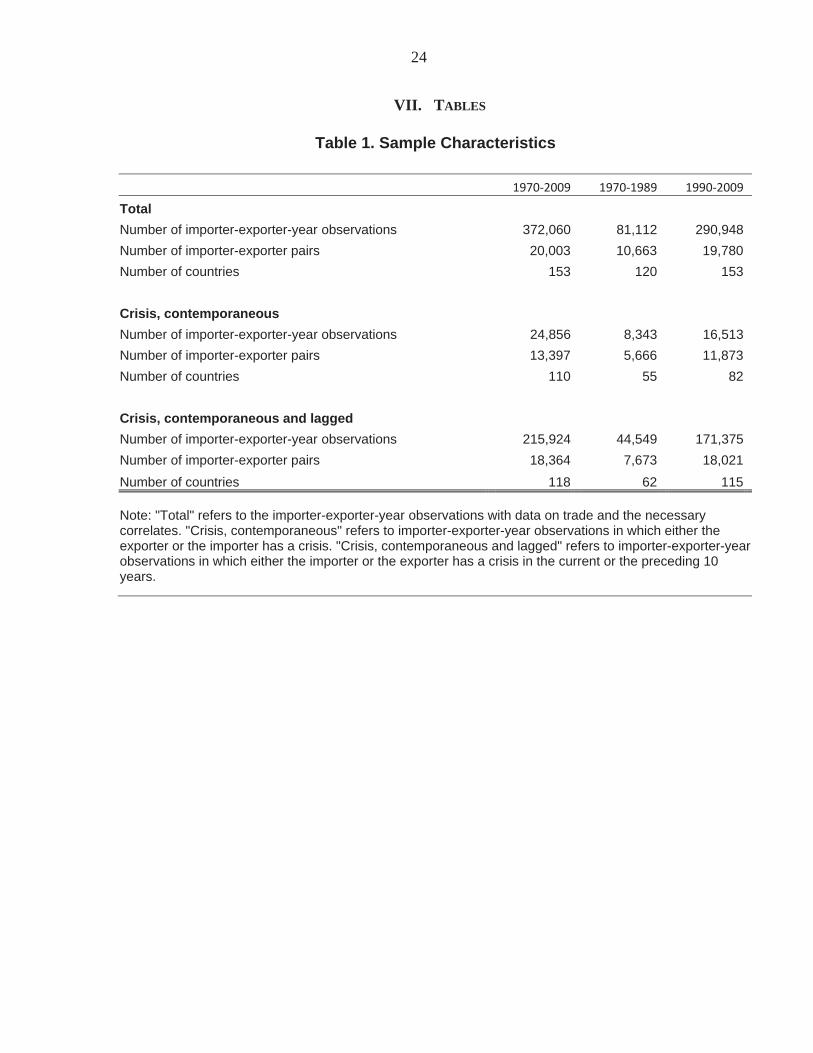
Table 1 presents some summary statistics on the observations, and frequency of crises. Our full sample contains 372,060 bilateral importer*exporter*year observations. Notice that instead of constructing trade flows by averaging exports and imports for each country pair, we use the unidirectional trade value and introduce both importer and exporter fixed effects. Thus, each country-pair which trades in both directions is represented twice: once for the imports from to and once for the imports from to . This gives us 20,003 importer*exporter pairs involving 153 countries. The bulk (two-thirds) of these observations is in the later sample period from 1990-2009. Summary statistics of all the variables used in the empirical analysis are provided in Table A1. Unlike war (see Glick and Taylor, 2010), crisis is not an infrequent occurrence in the data. Almost 7 percent of the observations in the sample involve a contemporaneous crisis in either the importing or exporting country.

Before proceeding to the gravity framework, we examine how imports and exports evolve following financial crises. Figure 4 presents a first look at the data: it plots the coefficients on the importer and exporter crisis indicators and their lags from a simple regression of bilateral trade flows on these indicators, importer*exporter and time dummies. On average, imports fall by about 11 percent in the crisis year. An additional drop of about 13 percent occurs the following year. Imports recover slowly in subsequent years, so that even 10 years after the crisis, they are about 5 percent below what would have been predicted in the absence of a crisis. The effect on exports is smaller and often statistically indistinguishable from zero. There is no sharp drop in exports in the short term; exports drop by only 3 percent on average at the onset of a crisis, and they recover quickly to their “normal” level within two years following the crisis.

In the next section, we analyze more formally whether, within the gravity framework of trade, crises continue to have lasting effects on imports and little effect on exports.

IV. GRAVITY FRAMEWORK RESULTS

A. Main Findings

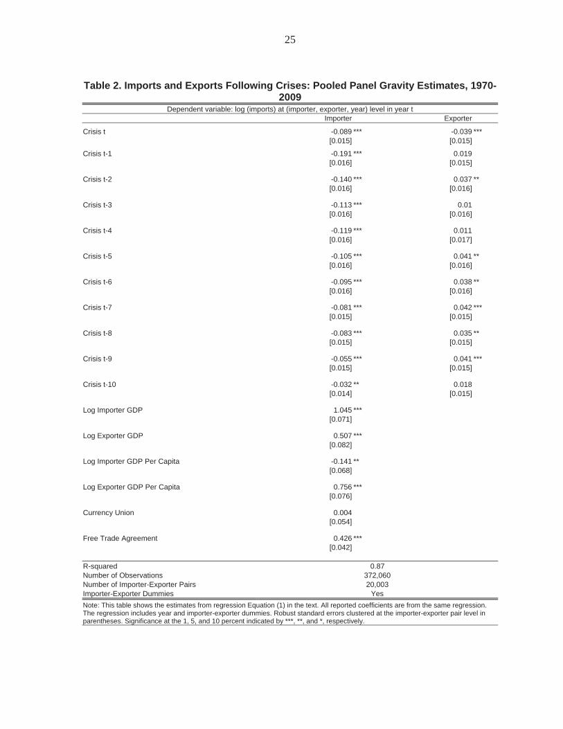
Table 2 presents estimates from the augmented gravity model of trade, using our preferred specification, equation (1). To account for potential autocorrelation and heteroskedasticity in the error term, standard errors are clustered at the importer*exporter level. Since the baseline specification includes importer*exporter fixed effects, the usual gravity time-invariant country-pair controls, such as distance, etc., are not included. We include the contemporaneous and lagged crisis indicators in the importer and exporter countries. The

10

number of lags was chosen by a top-down approach8: the estimated coefficients on crisis in the importing country become statistically insignificant after 10 lags. For brevity, the coefficients on the year and importer*exporter fixed effects are not reported.

Not surprisingly, the gravity model fits the data well, explaining about 87 percent of the variation in bilateral trade flows. The estimated coefficients on most of the importer- and exporter-time varying control variables such as GDP, currency union and FTA are plausible and similar to what has been found in the literature.

The key variables of interest are the importer and exporter crisis dummies and their lags, which capture the effect a crisis has on a country’s imports and exports during its onset and in the following 10 years, after controlling for the standard gravity determinants of trade (some of which are also affected by the crisis). These estimated coefficients and the 90 percent confidence interval around the estimated coefficients are also plotted in Figure 5.9

The estimated coefficients on contemporaneous and lagged importer crisis dummies are all negative and statistically significant at the one percent level (except the tenth lag, which is significant at the 5 percent level). The estimated effects are economically significant as well. On average, imports fall by 9 percent below the gravity-predicted level in the year of the crisis, and by further 10 percent in the following year. They recover slowly in subsequent years: 5 years after a crisis, imports are still 10 percent below normal. It takes more than 10 years for imports to get back to normal.10

How does the size of the fall in imports following a financial crisis compare with the trade disruption effect of other “shocks” that countries experience? The contemporaneous decline of imports following crises is comparable to the effect of violence on bilateral trade flows estimated by Blomberg and Hess (2006).11 For example, they find that a terrorist incident is associated with a 5 percent decline in a country’s trade, whereas revolutions and interethnic conflicts are associated with declines of 19 percent and 15 percent respectively. On the other hand, the average decline in imports following a crisis is much smaller than the destruction of trade between countries at war with each other as estimated by Glick and Taylor (2010). The contemporaneous effect of war on trade between belligerents is roughly nine times the effect of a financial crisis, though this comparison may not be appropriate since the latter measures the average effect on trade with all partners, and the former measures the effect on trade 8 Pedroni (2004), for example, illustrates the advantages of using a top-down approach for the selection of lag length in a panel setting.

9 The exact effect on imports in year can be calculated as ( , since is small.

10 More precisely, it takes 11 years, since the coefficient of the 11th lag is statistically indistinguishable from zero.

11 Blomberg and Hess (2006) examine only the contemporaneous effects of violence on trade.

11

between countries at war with each other. Perhaps a more suitable comparator is the average effect war has on “neutrals,” i.e., trading partners who are not directly involved in the conflict. Glick and Taylor find that trade with neutrals declines by about 12 percent on average at the onset of war, and that these effects remain statistically significant up to seven years after the start of the conflict. Thus, the magnitude of the effect of a war on neutrals is similar to a financial crisis.12

How does the loss in imports following a financial crisis compare with other impediments to trade, such as, for example, tariffs? We follow the methodology in Feenstra (2002) and Blomberg and Hess (2006) to estimate a “tariff equivalent.” The tariff equivalent for the

coefficient on the importer-crisis dummy in period is given by , where

is the elasticity of substitution between domestic and foreign goods and is the estimated effect of crisis on imports. As is common in the literature (e.g. Anderson and Van Wincoop, 2003), we calculate the tariff equivalent factors using values of equal to 5 or 10. The estimates are shown in Table 3. Based on our estimates, the tariff-equivalent cost of crisis in the importer country are between 1-2 percent in the year of the crisis and in the range of 2-5 percent in the year following the crisis. These costs are persistent and remain between 1-3 percent 5 years following the crisis. The contemporaneous tariff equivalent costs of terrorist incidents, revolutions and interethnic conflicts calculated by Blomberg and Hess (2006) are also in the range of 1-3 percent.

In contrast to imports, the evolution of exports following a crisis is much more muted. The estimated coefficients on the crisis dummy and its lags in Table 2 (and Figure 5) are often statistically insignificant and much smaller in magnitude. While there is a small drop in exports in the year of the crisis, exports recover quickly, and are back to their predicted level in the year following the crisis. If anything, exports hover slightly above their gravity predicted levels following financial crises.

The larger and more persistent losses in imports relative to exports are, indeed, striking. One possible explanation is that exports of a country are dependent on external demand, and as long as that is robust, we should not observe a deleterious effect of a crisis at home on exports. In fact, while lower domestic demand directly reduces import volumes, it may also reduce residents’ consumption of exportable goods, freeing up space for more exports.

The behavior of exports is also consistent with the large depreciation of the exchange rate accompanying many crises episodes. Figure 6a shows that on average, the US-dollar exchange rate depreciates by 72 percent in the year following the crisis episode, and it takes

12 Alternatively, we can compare the effect of war on trade between belligerents with the effect of a financial crisis on trade, when both importer and exporter are in crisis. The average trade loss between countries that are both in crisis over ten years is roughly half of that following a war. See Section V for details.

12

about 8 years for the exchange rate to get back to normal.13 Moreover, as we show in the robustness tests below, the rise in exports above the gravity-predicted levels observed in the medium-run becomes statistically indistinguishable from zero, once we control for exchange rates.

Why is there such a sharp negative effect of financial crises on imports and why is it so long lasting? One potential explanation could be that crises are associated with increased protectionism. In the aftermath of a crisis, interest groups that favor protecting domestic production may be strengthened.14 In order to evaluate this explanation, we explore how import tariffs and antidumping measures evolve following past crises. As shown in the top-left panel in Figure 6b, we do not find any evidence that protectionism, as measured by average tariffs, increases following a crisis. However, we do find some evidence for a small increase in the number of antidumping measures implemented following a crisis. On average, the number of antidumping measures increase by roughly 2 percent in the year following the crisis, then slowly decrease over time (top-right panel, Figure 6b).15 Although we do not find much evidence for increased protectionism as a potential mechanism through which crisis affects imports with these particular measures, increased protectionism may manifest itself in “murky” forms (e.g., clauses in stimulus packages that restrict spending to domestic producers), which are difficult to detect in the data.

Another potential channel through which crises may adversely affect imports is through changes in the volatility of exchange rate, which has been found to adversely affect trade (see IMF (2004) for a survey of the literature).16 In order to explore the importance of this mechanism, we look at how exchange rate volatility evolves following crises. Following the literature, we measure exchange rate volatility as the annual standard deviation of monthly changes in the exchange rate. Crises are indeed followed by substantial increases in the volatility of the exchange rate which declines over the medium-term (bottom-left panel, Figure 6b). On average, exchange rate volatility increases by almost half in the first two years following a crisis, and subsequently returns to normal. Hence, increased exchange rate

13 The evolution of the exchange rate following crises presented in Figure 6a as well as of the other mechanisms in Figure 6b is estimated by regressing the log of the dependent variable (f.ex. exchange rate) on a crisis indicator and its lags, country and year fixed effects.

14For example, the Great Depression was followed by a “wholesale rise in protectionism,” which not only slowed the process of economic recovery but created lasting protectionist legacies in a number of countries (see O’Rourke, 2009).

15 Average tariffs are from IMF (2008) and the number of antidumping measures implemented is from Bown (2010).

16 As discussed below, the import losses following crises persist even after controlling for the level of the exchange rate, which rules it out as a potential mechanism.

13

volatility could potentially be an important channel through which crises affect imports adversely in the short run.

Finally, another possible story is that the loss in imports following crises reflects adjustments in the number of imported varieties (rather than the volume of existing varieties), i.e., adjustment on the extensive margin. The underlying idea is that of a reverse “beachhead effect.”17 If large enough shocks (e.g., a crisis) cause firms to exit markets and reentry entails new sunk costs, a crisis could have a persistent effect on imports. In order to explore this possibility, we look at the evolution of the number of imported varieties. We define a variety as a product from a different country, measured at the 6-digit HS classification. We find some evidence for adjustment on the extensive margin. As shown in the bottom- right panel of Figure 6b, on average, there is a 7 percent reduction in the number of imported varieties in the year following the crises, which recovers only slowly.

B. Robustness

In what follows, we show that the main findings in Table 2 are robust to a number of changes in specification and additional controls. The robustness tests are shown in Table 4 and summarized in Figure 7.

Including bilateral country-pair variables

Instead of estimating eq. (1) with importer*exporter fixed effects, in the second column of Table 4 we present the traditional gravity specification which includes separate dummies for the exporter and importer, allowing us to estimate the coefficients on the standard time-invariant country-pair characteristics such as distance, a common land border, either or both partners being an island or landlocked, common legal origin, common language, and colonial ties. The main findings are robust to this alternative specification: imports fall substantially and persistently following crises, while exports are hurt less and recover quickly. The estimated coefficients on most other bilateral trade costs variables (not reported for brevity) are similar to what has been found in the literature. For example, greater physical distance reduces bilateral imports, whereas common land border, legal origin and colonial linkages enhance trade significantly.

Addressing omitted variable and selection biases

As in traditional estimates of the gravity equation, in the results presented above, we use only the sample of country-pairs that have positive bilateral imports. Helpman, Melitz and Rubinstein (2008) (henceforth, HMR) argue that such standard estimation of the gravity

17See Baldwin (1988), who proposed beachhead effects as one potential explanation for hysteresis in international trade. The argument is that firms that have incurred the sunk costs of entering a relationship will not leave simply because conditions turn bad.

14

equation is subject to two types of potential biases: a sample selection bias (owing to zero trade flows), and a bias from potential asymmetries in trade (i.e. one country imports from, but does not export to, the other country).18 They show that the latter bias is due to an omitted variable that measures the impact of the number (fraction) of exporting firms, i.e. the extensive margin of trade. HMR develop a two-step empirical methodology to address these potential biases and suggest that this procedure yields consistent estimates of the parameters of the gravity equation. Following their methodology, we first estimate a probit regression including an index for common religion (which serves as the exclusion variable for the second step). Predicted components of this equation are then used in the second stage to estimate the gravity equation, which excludes the religion variable. The results are shown in column 3 of Table 4. Note that we implement the HMR methodology in the specification with separate exporter and importer fixed effects (and not interaction), since the exclusion variable varies only across country-pairs but not over time. The estimated coefficients of the crisis dummies are similar to those in column 1.19

Varying the elasticity of imports with respect to GDP

In the baseline specification, we assume a constant elasticity of imports with respect to GDP. However, it is possible that imports may be more responsive to cyclical than to trend movements in output; if so, the baseline approach would overestimate the fall in imports controlling for GDP. To test this, we allow the elasticity of imports to vary across the trend and cyclical components of output, where the trend and cycle were separated using a Hodrick-Prescott filter. The estimated coefficients on the crisis dummies (column 4, Table 4) are almost identical to the baseline specification.

In a similar vein, the sensitivity of imports to output may be particularly high in times of crisis. We thus allow the coefficient on GDP to vary during crisis and non-crisis periods. The estimated coefficients are shown in column 5 of Table 4. The total effect of a crisis on imports or exports in this case would include the interaction term between GDP and the crisis dummies. Evaluated at the average sample GDP for the crisis episodes, the total effect of a crisis on imports and exports is similar to the baseline specification (see Figure 7).

Controlling for changes in domestic aggregate demand

According to the theoretical underpinnings of the gravity equation, imports of country from country are a function of country ‘s domestic absorption (which determines its import

18 In our sample, half of the potential importer-exporter-year observations have zero trade flows, and 14 percent of the country-pair-year observations trade in only one direction.

19 When interpreting the findings of this robustness check, it is important to keep in mind that HMR methodology is more suitable for estimating the cross-sectional, rather than time-varying, determinants of trade, since their exclusion variable (common religion) is time-invariant.

15

demand), and domestic output in country (which proxies for export supply). While GDP in the exporting country may be a reasonable proxy for its supply, GDP in the importing country may not be a good proxy for the absorption, especially during crisis periods. To the extent that absorption declines more than GDP during crises, the estimated import losses controlling for GDP may be overstated. In order to address this concern, in estimating the gravity equation, we replace GDP in the importing country by domestic absorption using data on absorption (the sum of consumption and investment expenditures), wherever available from the IFS. The main findings are robust to controlling directly for the importer’s absorption as presented in column 6 of Table 4.

Controlling for exchange rates and relative prices

Import dynamics may differ after crises due to changes in the exchange rates and relative price levels. We augment equation (1) to control for changes in the bilateral exchange rate and the relative price levels of the importer and exporter.20 The relative price is proxied by GDP deflator. The estimated effect of crisis on imports (column 7, Table 5) is very similar to the baseline specification in column 1. The estimated effect of the crisis on exports, on the other hand, is smaller, and is mostly insignificant apart from in the crisis year itself; in other words, some of the postcrisis improvement in export performance is explained by accompanying changes in the exchange rate.

Excluding episodes accompanied by currency crises, and recent crises

In order to address the concern that our findings may be driven only by large depreciations accompanying financial crises, we isolate only those episodes which did not coincide with currency crises (as defined by Laeven and Valencia, 2008) in the year of the financial crisis or the year before. The specification is identical to the baseline equation (1), but focuses only on “pure” financial crises. The estimated coefficients on the crisis dummies shown in column 8 of Table 4 are once again similar to the baseline specification.21

Are our baseline results for the short-term behavior of trade driven by the most recent episodes of financial crises, whose effects on trade were particularly large? In order to address this issue, we restrict the dataset to 2006, excluding the 13 most recent episodes of banking crises, which occurred primarily in advanced countries like the U.S., the United Kingdom, and Germany. The results are shown in column 9 of Table 4. The magnitude of the 20 The estimated coefficients on the crisis dummies are very similar when we use the real effective exchange rate rather than the bilateral exchange rates.

21 There are a quarter of the financial crisis episodes which were accompanied by a currency crisis in the same or previous year. If we widen the window to episodes accompanied by a currency crisis two years before or after the crisis, then roughly half of the financial crisis episodes are accompanied by a currency crisis. The estimated coefficients on crisis dummies are similar if we define the “pure” crisis episodes based on this wider window.

16

import losses in the short run is indeed smaller once we omit the recent episodes. For example, imports are 7 percent and 17 percent below predicted in the year of the crisis and the following year respectively, compared to 9 percent and 19 percent, respectively, in the baseline. Similarly, export losses in the year of the crisis are even more muted once we omit the recent episodes. Nonetheless, it is clear that our main findings are not driven by the recent wave of banking crises.

Allowing the multilateral resistance term to vary over time

In the baseline specification described in equation (1), the multilateral trade resistance term is captured by , the importer-exporter pair dummies. , however, is time-invariant, and thus controls only for those multilateral trade costs which do not vary over time. We estimate an alternative specification where we allow the ’s to vary by decade. The estimated coefficients on the crisis dummies from this more general specification are shown in column 10 of Table 4. The results are qualitatively similar to the baseline specification (1).

Examining aggregate rather than bilateral trade

Finally, we look at the evolution of aggregate imports or exports of a country following a financial crisis. We estimate a collapsed version of the gravity model where we aggregate imports or exports of a country across all its trading partners. Notice that while equation (1) puts equal weight on all trading partners, the collapsed version puts more weight on larger trading partners, and is analogous to estimating (1) weighted by size of the partner. The estimating equation for the collapsed gravity model is specified as follows:

(2) Where stands for imports or exports, and represent partners’ trade-weighted GDP and per capita GDP respectively. We first estimate eq. (2) with imports as the dependent variable. The estimated coefficients on the crisis dummies are shown in the top rows of column 11 of Table 4. The magnitude of the crisis coefficients declines to about half relative to the baseline, but continues to be statistically significant. Aggregate imports fall by 9 percent in the year following the crisis, and then recover slowly. Imports are 6 percent below predicted 5 years following the crisis, and recover to normal in 10 years.22 Similarly, we

22 In order to explore this finding further, we estimated Equation (1) allowing the coefficients on crisis dummies to vary by size of the partner. Consistent with the findings from the collapsed gravity specification, we find that

(continued…)

17

estimate (2) with aggregate exports as the dependent variable. The coefficients on the exporter crisis dummies are shown in the bottom half of the same column 11 of Table 4. Aggregate exports do not deviate significantly from normal either in the short or medium term.

To summarize, a number of robustness tests support the main finding that financial crises are associated with a persistent decline in imports, while exports are not as adversely affected. The various robustness tests are summarized in Figure 7, which clearly shows that the evolution of imports and exports under the various robustness tests are remarkably similar.23

Endogeneity issues

Although our findings are robust to the introduction of a number of controls and alternative specifications, there is still a concern that our estimates might be biased due to endogeneity and in particular, reverse causality. For example, the occurrence of a crisis may be affected by the behavior of trade. Alternatively, the effects we have documented could be driven by underlying factors that may also have affected the likelihood of a crisis. While being far from definitive, we try to shed some light on this issue using a few simple methods following Cerra and Saxena (2008). First, we drop contemporaneous crisis episodes which are more likely to be endogenous to the behavior of trade. Second, we augment equation (1) to include lags of GDP as predictors of a crisis. Finally, we control for lags of imports to address reverse causality concerns.24 The results are shown in columns 2-4 of Table 5 and in Figure 8. The estimated coefficients on the crisis indicators are almost identical to the baseline specification. Notice that the total effect of a crisis in the specification with lags of imports includes not only the direct effects indicated by the estimated coefficients in Table 5, but also the indirect effects through the dynamics of the model.25

imports from small trading partners are hit more following a crisis. Imports from large trading partners seem to be more resilient to a crisis (large trading partners defined as top 20 in terms of imports).

23 For robustness, we also examined whether import losses are a feature only of severe crises, where a severe crisis is defined as an episode in which the size of the output loss in the first two years of the crisis is above the median. We found that import losses occur regardless of whether a financial crisis is severe or moderate, although the initial import loss is larger for severe crises.

24 The presence of country fixed effects and lagged dependent variables may lead to inconsistent estimates. However, Nickell (1981) shows that the order of the bias is 1/T, which is small for our sample. Also, Judson and Owne (1999) show that the bias of the fixed effect estimator is approximately 2-3 percent on the lagged dependent variable and less than 1 percent on other regressors for a panel of size N=100, T=30, and low persistence.

25 In order to directly test for feedback effects, we also estimate a very simple specification where we look at whether the evolution of aggregate trade in the current or previous year drives the occurrence of a crisis episode. We find little evidence of feedback effects.

18

To summarize, the simple controls for endogeneity presented in Table 5 and Figure 8 are far from definite but nonetheless show a picture that is consistent with our baseline results. The main goal of the paper is to document stylized facts on the evolution of trade following past episodes of financial crisis. To the extent that crisis in general is not exogenous, our estimates could capture the effect of the crisis on imports and exports or any underlying factor that may have led to it.26

V. DIFFERE CES I TRADE DY AMICS ACROSS PRODUCTS, DURI G GLOBAL DOW TUR S, A D OVER TIME

Until now, the reported estimates represent averages of the effect of crises on trade across all products, time periods and trading partners in the sample. In this section, we analyze whether the effect of a crisis varies systematically across (i) product categories, (ii) global downturns and (iii) over time.

A. Do Postcrisis Trade Dynamics Vary Across Products?

It is well known that the extent of the trade collapse during the 2008-09 global downturn differed across different product categories. The largest collapse was in demand for “postponable” items such as capital and consumer durables.27 Is this pattern also borne out in earlier crises? In order to explore the evolution of imports in different product categories, we estimate a product-level gravity regression. We consider four product categories—consumer nondurables, capital and consumer durables, intermediate and primary goods.28

We follow Harrigan (2003) in stacking the product categories together, and estimating a gravity specification with product fixed effects. In addition, we allow all the standard gravity controls to vary by product categories. The estimating equation is specified as follows:

26 We also conduct a simple falsification test to check whether the results are driven by something specific to financial crises, or are the results driven by some omitted variables which are common to recessions in general. We estimate equation (1) replacing the crisis variable with episodes of recession, where recessions are defined by the start-year using the Braun-Larrain (2005) methodology. The recession dummies, in general, have little effect of imports and exports. There is a small (3-4 percent) negative and statistically significant effect on imports in the year of the recession and the following years, and no significant effect thereafter. The results provide further evidence that our main findings are specific to financial crises and may not be driven by omitted variables that characterize recessions in general.

27 For example, see Bems, Johnson and Yi (2010).

28 Data on imports and exports by product category are constructed from the NBER-UN World Trade Flows database (see Feenstra et al, 2005). The data base is first extended using the UN Comtrade database. The Standard International Trade Classification, Revision 2 (SITC Rev. 2) codes that identify products in the NBER-UN trade data are matched to the UN Broad Economic Classification (BEC) codes. These are then classified into Capital Goods, Consumer Durables, Consumer Non Durables, Intermediate Goods and Primary Goods, following Pula and Peltonen (2009).

19

(3)

Where denotes the product category, and denotes the vector of product fixed effects and denotes the triple interaction of importer, exporter and product fixed effects.29

The estimated coefficients from equation (3) are presented in Table 6, and the evolution of imports and exports in different product categories is summarized in Figure 9. As in the recent global downturn, capital and consumer durables experience the largest short-term drop, with an average drop of 23 percent in the year after a crisis. The recovery in imports for this product category is protracted, with durables imports remaining 16 percent below normal after 5 years. Intermediate products are also quite adversely affected, with imports in this category remaining 21 percent below predicted in the year after crisis, and recovering only slowly in the medium-term. Consumer non-durables also experience smaller but still significant drops in the short (13 percent in the year following the crisis) and medium term (8 percent below predicted after 5 years).30 Finally, imports of primary goods seem to be least affected by a crisis.

Exports of all product categories are much less affected than imports, with all categories except primary goods recovering in the year after the crisis. Capital and consumer durables experience the sharpest decline in the year of the crisis (5 percent), but recover quickly. The decline in exports of primary goods though marginally smaller in magnitude on impact, is more persistent—recovering to normal 3 years after the crisis.31

29 Harrigan (1996) shows that product fixed effects can be derived from a model of differentiated goods and home bias in demand, where the degree of home bias differs by products. In the absence of product-specific intercepts, the product-level gravity regression can be summed over products to give the aggregate equation in (1), and which has served the basis of innumerable studies.

30For past crises that typically occurred in lower-income countries with weak social safety nets, it is possible that crises and the resulting (uncushioned) rise in unemployment would lead to declines even in consumer non-durables. See for example Friedman and Levinsohn (2003) for an analysis of the impact of the 1997 Asian crisis on Indonesian households. The effects would remain even in the regressions which control for output, if the measured GDP decline failed to adequately capture the adverse impact on poorer households. 31 Primary goods also experience the smallest increase in exports above gravity-predicted in the medium-term. This could be explained by the fact that primary goods include commodities, which are often priced in foreign currency. Hence, the exchange rate depreciation associated with the crisis does not boost exports to an extent similar to other product categories. See Cook and Devereux (2006) for evidence on foreign currency pricing in the case of Asia.

20

B. Are Postcrisis Trade Dynamics Different During Global Downturns?

In the baseline regression equation (1), we include year fixed effects to control for factors that affect all countries’ trade simultaneously, such as global downturns or increases in global uncertainty or risk aversion. Hence, the effect of financial crises captured in the baseline specification is over and beyond whatever effect global downturns have on world trade. However, our empirical framework allows us to evaluate whether trade dynamics differ if a crisis coincides with a global downturn. We interact contemporaneous and lagged crisis dummies with indicators of whether the year of the episode coincided with a global downturn. We define years of global downturn as in Freund (2009).32 About a fifth of the crisis episodes in our sample occurred during global downturns.

The estimating equation is specified as follows:

(4)

Where =1 if a global downturn occurred in year .

The effect of a crisis on a country’s imports, years following the crisis is captured by coefficient if the year of the crisis does not coincide with a global downturn, and is equal to if the crisis is accompanied by a global downturn. The coefficients on the crisis dummies and the 90 percent confidence intervals are summarized in Figure 10. Countries that experience a crisis during a global downturn have deeper import and export losses, even after conditioning on all the standard gravity controls. More specifically, the imports of a crisis country fall 28 percent below predicted in the year following the crisis, almost 10 percentage points higher than a crisis episode which is not accompanied by a downturn. Just as important, the decline is much more persistent if the crisis is accompanied by a global downturn; imports remain almost 10 percent below normal even ten years after a crisis. Exports also fall more, and take longer to recover for crises accompanied by global downturns; however, the evolution of exports continues to be much less dramatic compared to imports, and frequently remains statistically indistinguishable from zero. These findings

32Specifically, Freund (2009) defines global downturns as years where world real GDP growth is (i) below 2 percent, (ii) more than 1.5 percentage points below the previous 5-year average, and (iii) at its minimum relative to the previous two years and the following two years. The following global downturns are identified by this procedure: 1975, 1982, 1991, 2001, and 2008.

21

suggest that the recent financial crises may result in deeper trade losses than historical episodes which did not coincide with a global downturn.

Furthermore, we look more specifically at whether the effect of a financial crisis in a country is more severe when it is concurrent with a crisis in only the trading partner (rather than the case of a global downturn discussed above). We augment equation (1) with another indicator variable which equals one if the crisis occurs in both the importer and the exporter. We estimate the following regression equation:

(5)

Where if the crisis occurs in both country i and country j in year t-k. Note

that the effect of a crisis in both the importing and exporting countries on the trade flows

between these two countries is given by . The estimated coefficients and the

confidence intervals are summarized in Figure 11. It is indeed the case that the decline in

trade between two countries that have both had a crisis is disproportionately more severe, as

well as more persistent. Five years following the crisis, for example, the imports of a country

from trading partners that also had a crisis are more than 30 percent below normal. In

comparison, as shown in Figure 4, its imports from other countries are only 10 percent below

normal.

C. Do Postcrisis Trade Dynamics Vary Over Time?

Finally, we examine whether trade has become more or less resilient to crises over time. One possible conjecture is that there has been a trend towards greater production sharing over time and that this has made trade more resilient. The underlying idea is that of a “beachhead effect,” discussed above, where firms that have incurred the sunk costs of entering a relationship will not leave simply because conditions turn bad.

In order to explore this hypothesis, we look at the evolution of trade following crises pre- and post-1990. We interact the crisis dummies with an indicator for whether the episode occurred after 1990. The evidence presented in Figure 12 suggests that trade has indeed become more resilient over time. During the post-1990 episodes, imports are 16 percent below normal in the year following a crisis, and are almost back to normal levels just three years after the crisis. The pre-1990 episodes are relatively more severe. The maximum decline is as much as 21 percent, and imports are still 6 percent below predicted after 10 years. Export losses are

22

also typically higher for the pre-1990 episodes. During the post-1990 episodes, the behavior of exports seems to be completely explained by standard gravity controls.

Our findings are consistent with other studies, such as Altomonte and Ottaviano (2009), who note the resilience of trade between western and central Europe during the recent crisis and conjecture that this is due to the strengthened production linkages between the two regions, and Bernard et al. (2009), who document the resilience of intra-Asian “supply chain” trade following the Asian crisis.

VI. CO CLUSIO S

Using bilateral trade data for a large set of countries over the period 1970-2009, this paper provides evidence that financial crises are associated with large and persistent losses in imports. This is over and above any import compression due to lower output and changes in other standard determinants of trade flows as a result of a crisis. In contrast, exports are not as adversely affected and their behavior can be explained by standard gravity determinants. We also find that imports of consumer and capital durables are hit the most; episodes coinciding with global downturns and those concurrent with a crisis in the partner countries, have more adverse effects; and trade has tended to become more resilient over time.

Why do crises have a persistent effect on imports? While establishing the mechanisms behind our findings is beyond the scope of this paper, we offer several possible conjectures. One possible explanation is a rise in protectionism following past crises. Although we do not find much evidence for a large increase in tariffs or antidumping measures following past episodes, we cannot rule out a rise in more hidden forms of protectionism following past crises, which are difficult to quantify.33 Another possible channel we explore is a rise in exchange rate volatility, which has been shown to adversely affect trade (e.g., Thursby and Thursby, 1987). There is indeed a significant increase in the volatility of the exchange rate in the short term that declines over the medium term. Finally, we offer some evidence to suggest that the fall in imports after a crisis reflects an adjustment on the extensive margin, i.e. countries significantly reduce the number of imported varieties.

One important hypothesis that we are unable to test is whether “composition effects”—large drops in demand for goods that constitute a larger share of trade than of output—can explain trade dynamics in past financial crises. Eaton et al (2010) and Levchenko et al. (2010) find that composition effects can account for the bulk of the disproportionate decline in trade relative to output in the 2008-09 global downturn. Unfortunately, the lack of comprehensive historical data on the composition of demand for various categories of goods precludes a detailed investigation of this particular mechanism, so we leave this for future research.

33 See Gregory et al. (2010) for a discussion on “behind the border” measures —such as technical barriers to trade, procurement, and regulatory measures—in the context of the 2008-09 crisis.

23

Although caution should be exercised when drawing implications from historical crisis episodes for the recent crisis, given its severity and its global nature, the findings of this paper could be used to shed light on where trade might be headed. The recent financial crisis has been concentrated in many large, advanced economies that account or almost of global demand. The findings in this paper are consistent with the sharp and substantial drop in import demand that occurred in countries that recently went through a financial crisis. And if past experience is any guide, imports of these countries are likely to remain below normal—i.e, below where they would have been in the absence of a crisis—for a protracted period.

24

VII. TABLES

Table 1. Sample Characteristics

1970-2009 1970-1989 1990-2009

Total Number of importer-exporter-year observations 372,060 81,112 290,948Number of importer-exporter pairs 20,003 10,663 19,780Number of countries 153 120 153

Crisis, contemporaneous Number of importer-exporter-year observations 24,856 8,343 16,513Number of importer-exporter pairs 13,397 5,666 11,873Number of countries 110 55 82

Crisis, contemporaneous and lagged Number of importer-exporter-year observations 215,924 44,549 171,375Number of importer-exporter pairs 18,364 7,673 18,021Number of countries 118 62 115

Note: "Total" refers to the importer-exporter-year observations with data on trade and the necessary correlates. "Crisis, contemporaneous" refers to importer-exporter-year observations in which either the exporter or the importer has a crisis. "Crisis, contemporaneous and lagged" refers to importer-exporter-year observations in which either the importer or the exporter has a crisis in the current or the preceding 10 years.

25

Table 2. Imports and Exports Following Crises: Pooled Panel Gravity Estimates, 1970-

2009Dependent variable: log (imports) at (importer, exporter, year) level in year t

Importer Exporter

Crisis t -0.089 *** -0.039 *** [0.015] [0.015]

Crisis t-1 -0.191 *** 0.019[0.016] [0.015]

Crisis t-2 -0.140 *** 0.037 ** [0.016] [0.016]

Crisis t-3 -0.113 *** 0.01[0.016] [0.016]

Crisis t-4 -0.119 *** 0.011[0.016] [0.017]

Crisis t-5 -0.105 *** 0.041 ** [0.016] [0.016]

Crisis t-6 -0.095 *** 0.038 ** [0.016] [0.016]

Crisis t-7 -0.081 *** 0.042 *** [0.015] [0.015]

Crisis t-8 -0.083 *** 0.035 ** [0.015] [0.015]

Crisis t-9 -0.055 *** 0.041 *** [0.015] [0.015]

Crisis t-10 -0.032 ** 0.018[0.014] [0.015]

Log Importer GDP 1.045 *** [0.071]

Log Exporter GDP 0.507 *** [0.082]

Log Importer GDP Per Capita -0.141 ** [0.068]

Log Exporter GDP Per Capita 0.756 *** [0.076]

Currency Union 0.004[0.054]

Free Trade Agreement 0.426 *** [0.042]

R-squared 0.87 Number of Observations 372,060 Number of Importer-Exporter Pairs 20,003 Importer-Exporter Dummies Yes Note: This table shows the estimates from regression Equation (1) in the text. All reported coefficients are from the same regression. The regression includes year and importer-exporter dummies. Robust standard errors clustered at the importer-exporter pair level in parentheses. Significance at the 1, 5, and 10 percent indicated by ***, **, and *, respectively.

26

Table 3. Tariff Equivalent Trade Costs

[1] [2] Sigma=5 Sigma=10 Importer Importer Crisis t 2.2 1.0 Crisis t-1 4.9 2.1 Crisis t-2 3.6 1.6 Crisis t-3 2.9 1.3 Crisis t-4 3.0 1.3 Crisis t-5 2.7 1.2 Crisis t-6 2.4 1.1 Crisis t-7 2.0 0.9 Crisis t-8 2.1 0.9 Crisis t-9 1.4 0.6 Crisis t-10 0.8 0.4 Notes. The tariff-equivalent trade costs shown in this table are calculated using the coefficients in Table 2. Each number represents a tariff-equivalent percentage; i.e. the percent by which tariffs have to be raised to reduce imports by the same amount as occurrence of a crisis. The first column is based on a CES elasticity of 5, while the last column is based on a CES elasticity of 10. See text for details of the calculations.

26

Tabl

e 4.

Impo

rts

and

Expo

rts

Follo

win

g C

rises

: Rob

ustn

ess

Bas

elin

e

Cou

ntry

-P

air

Con

trols

H

MR

C

yclic

al/T

rend

E

last

icity

C

risis

A

ggre

gate

D

eman

d

Exc

hang

e ra

te a

nd

pric

es

No

Cur

renc

y C

risis

at t

-1

or t

No

2007

-20

09

cris

es

vary

m

ultil

ater

al

resi

stan

ce

Agg

rega

te

(1

)

(2)

(3

)

(4)

(5

)

(6)

(7

)

(8)

(9

)

(10)

(1

1)

Impo

rter:

Cris

is t

-0.0

89 **

* -0

.058

***

-0.0

47**

*-0

.089

***

-0.0

85**

*-0

.125

***

-0.1

00**

*-0

.045

***

-0.0

68**

*-0

.045

***

-0.0

4[0

.015

] [0

.017

][0

.017

][0

.015

][0

.015

][0

.016

] [0

.015

][0

.017

][0

.016

][0

.014

][0

.028

]Im

porte

r: C

risis

t-1

-0.1

91 **

* -0

.146

***

-0.1

36**

*-0

.19

***

-0.1

88**

*-0

.224

***

-0.1

93**

*-0

.144

***

-0.1

69**

*-0

.154

***

-0.0

86**

[0.0

16]

[0.0

18]

[0.0

18]

[0.0

16]

[0.0

16]

[0.0

16]

[0.0

15]

[0.0

17]

[0.0

17]

[0.0

15]

[0.0

33]

Impo

rter:

Cris

is t-

2 -0

.14

***

-0.1

19**

*-0

.109

***

-0.1

4**

*-0

.141

***

-0.1

75 **

* -0

.157

***

-0.0

91**

*-0

.127

***

-0.1

24**

*-0

.081

**[0

.016

] [0

.019

][0

.019

][0

.016

][0

.016

][0

.017

] [0

.016

][0

.018

][0

.017

][0

.017

][0

.035

]Im

porte

r: C

risis

t-3

-0.1

13 **

* -0

.099

***

-0.0

93**

*-0

.114

***

-0.1

14**

*-0

.15

***

-0.1

10**

*-0

.072

***

-0.1

04**

*-0

.100

***

-0.0

54*

[0.0

16]

[0.0

19]

[0.0

19]

[0.0

16]

[0.0

16]

[0.0

17]

[0.0

15]

[0.0

18]

[0.0

16]

[0.0

18]

[0.0

30]

Impo

rter:

Cris

is t-

4 -0

.119

***

-0.1

02**

*-0

.102

***

-0.1

19**

*-0

.117

***

-0.1

6 **

* -0

.130

***

-0.0

88**

*-0

.114

***

-0.1

04**

*-0

.055

**[0

.016

] [0

.019

][0

.019

][0

.016

][0

.016

][0

.017

] [0

.015

][0

.018

][0

.017

][0

.018

][0

.028

]Im

porte

r: C

risis

t-5

-0.1

05 **

* -0

.088

***

-0.0

9**

*-0

.105

***

-0.1

05**

*-0

.158

***

-0.1

22**

*-0

.063

***

-0.1

07**

*-0

.100

***

-0.0

58**

[0.0

16]

[0.0

19]

[0.0

18]

[0.0

16]

[0.0

16]

[0.0

17]

[0.0

15]

[0.0

18]

[0.0

16]

[0.0

17]

[0.0

29]

Impo

rter:

Cris

is t-

6 -0

.095

***

-0.0

96**

*-0

.101

***

-0.0

95**

*-0

.094

***

-0.1

35 **

* -0

.103

***

-0.0

53**

*-0

.093

***

-0.0

89**

*-0

.063

**[0

.016

] [0

.018

][0

.018

][0

.016

][0

.016

][0

.017

] [0

.015

][0

.018

][0

.016

][0

.017

][0

.029

]Im

porte

r: C

risis

t-7

-0.0

81 **

* -0

.079

***

-0.0

84**

*-0

.081

***

-0.0

77**

*-0

.119

***

-0.0

87**

*-0

.057

***

-0.0

87**

*-0

.074

***

-0.0

63**

[0.0

15]

[0.0

18]

[0.0

18]

[0.0

15]

[0.0

15]

[0.0

16]

[0.0

15]

[0.0

17]

[0.0

16]

[0.0

17]

[0.0

27]

Impo

rter:

Cris

is t-

8 -0

.083

***

-0.0

75**

*-0

.083

***

-0.0

83**

*-0

.083

***

-0.1

24 **

* -0

.082

***

-0.0

79**

*-0

.084

***

-0.0

98**

*-0

.064

**[0

.015

] [0

.018

][0

.018

][0

.015

][0

.015

][0

.016

] [0

.014

][0

.017

][0

.016

][0

.016

][0

.025

]Im

porte

r: C

risis

t-9

-0.0

55 **

* -0

.054

***

-0.0

58**

*-0

.056

***

-0.0

54**

*-0

.1 **

* -0

.065

***

-0.0

64**

*-0

.071

***

-0.0

75**

*-0

.049

**[0

.015

] [0

.017

][0

.017

][0

.015

][0

.015

][0

.015

] [0

.014

][0

.017

][0

.016

][0

.015

][0

.024

]Im

porte

r: C

risis

t-10

-0

.032

**

-0.0

36**

-0

.043

***

-0.0

32**

-0.0

28**

-0.0

63 **

* -0

.030

**-0

.051

***

-0.0

47**

*-0

.042

***

-0.0

21[0

.014

] [0

.017

][0

.017

][0

.014

][0

.014

][0

.015

] [0

.013

][0

.016

][0

.015

][0

.014

][0

.022

]E

xpor

ter:

Cris

is t

-0.0

39 **

* 0.

009

0.01

8-0

.044

***

-0.0

38**

*-0

.037

**

-0.0

66**

*-0

.057

***

-0.0

010.

069

***

0.01

8[0

.015

] [0

.017

][0

.017

][0

.015

][0

.015

][0

.015

] [0

.014

][0

.016

][0

.017

][0

.015

][0

.033

]E

xpor

ter:

Cris

is t-

1 0.

019

0.07

***

0.07

8**

*-0

.001

0.02

10.

015

0.00

40.

012

0.05

8**

*0.

120

***

0.05

1*

[0.0

15]

[0.0

18]

[0.0

18]

[0.0

16]

[0.0

15]

[0.0

16]

[0.0

15]

[0.0

16]

[0.0

17]

[0.0

17]

[0.0

31]

Exp

orte

r: C

risis

t-2

0.03

7 **

0.

078

***

0.08

1**

*0.

026

0.03

7**

0.03

6 **

0.

015

0.03

3*

0.06

6**

*0.

118

***

0.04

6[0

.016

] [0

.019

][0

.019

][0

.016

][0

.016

][0

.017

] [0

.016

][0

.018

][0

.017

][0

.019

][0

.035

]E

xpor

ter:

Cris

is t-

3 0.

01

0.04

8**

0.

052

***

0.01

0.00

70.

01

-0.0

180.

018

0.03

1*

0.08

6**

*0.

028

[0.0

16]

[0.0

19]

[0.0

19]

[0.0

16]

[0.0

16]

[0.0

17]

[0.0

16]

[0.0

18]

[0.0

17]

[0.0

20]

[0.0

37]

Exp

orte

r: C

risis

t-4

0.01

1 0.

049

**

0.04

8**

0.

015

0.01

10.

008

-0.0

010.

007

0.02

70.

102

***

0.02

7[0

.017

] [0

.019

][0

.019

][0

.017

][0

.016

][0

.017

] [0

.016

][0

.019

][0

.017

][0

.020

][0

.038

]E

xpor

ter:

Cris

is t-

5 0.

041

**

0.06

6**

*0.

064

***

0.04

5**

*0.

037

**0.

035

**

0.02

20.

043

**0.

05**

*0.

126

***

0.03

[0.0

16]

[0.0

19]

[0.0

19]

[0.0

16]

[0.0

16]

[0.0

17]

[0.0

15]

[0.0

18]

[0.0

17]

[0.0

20]

[0.0

37]

27

Exp

orte

r: C

risis

t-6

0.03

8 **

0.

076

***

0.07

3**

*0.

042

***

0.03

4**

0.03

5 **

0.

023

0.03

7**

0.04

1**

0.

125

***

0.01

4[0

.016

] [0

.018

][0

.018

][0

.016

][0

.015

][0

.016

] [0

.015

][0

.018

][0

.016

][0

.020

][0

.033

]E

xpor

ter:

Cris

is t-

7 0.

042

***

0.06

5**

*0.

066

***

0.04

***

0.04

1**

*0.

036

**

0.02

7*

0.06

6**

*0.

033

**

0.12

8**

*0.

01[0

.015

] [0

.018

][0

.018

][0

.015

][0

.015

][0

.016

] [0

.015

][0

.017

][0

.016

][0

.020

][0

.031

]E

xpor

ter:

Cris

is t-

8 0.

035

**

0.05

6**

*0.

056

***

0.03

2**

0.03

4**

0.03

3 **

0.

026

* 0.

044

**0.

023

0.10

8**

*-0

.001

[0.0

15]

[0.0

18]

[0.0

18]

[0.0

15]

[0.0

15]

[0.0

16]

[0.0

15]

[0.0

17]

[0.0

16]

[0.0

19]

[0.0

30]

Exp

orte

r: C

risis

t-9

0.04

1 **

* 0.

057

***

0.06

1**

*0.

035

**0.

043

***

0.03

8 **

0.

019

0.05

8**

*0.

018

0.09

6**

*-0

.019

[0.0

15]

[0.0

17]

[0.0

17]

[0.0

15]

[0.0

14]

[0.0

15]

[0.0

14]

[0.0

17]

[0.0

16]

[0.0

17]

[0.0

32]

Exp

orte

r: C

risis

t-10

0.

018

0.02

0.02

60.

014

0.02

00.

018

0.00

20.

034

**-0

.011

0.06

2**

*-0

.006

[0.0

15]

[0.0

17]

[0.0

17]

[0.0

15]

[0.0

14]

[0.0

15]

[0.0

14]

[0.0

16]

[0.0

16]

[0.0

16]

[0.0

32]

R

-squ

ared

0.

87

0.74

0.

74

0.87

0.

87

0.87

0.

89

0.87

0.

87

0.88

0.

98

Num

ber o

f Obs

erva

tions

37

2,06

0 29

1,76

429

8,06

737

2,06

029

1,76

434

0,30

2 32

3,06

137

2,06

032

2,97

037

2,06

04,

156

Num

ber o

f Im

porte

r-E

xpor

ter P

airs

20

003

13

632

13

918

20

003

13

632

18

457

18

029

20

003

19

961

20

003

Not

e: A

ll re

gres

sion

s ex

cept

(2),

(3) a

nd (1

1) in

clud

e ye

ar a

nd im

port-

expo

rter p

air d

umm

ies.

Rob

ust s

tand

ard

erro

rs c

lust

ered

at t

he im

porte

r-ex

porte

r pai

r lev

el in

par

enth

eses

in a

ll re

gres

sion

s ex

cept

(11)

. Sig

nific

ance

at t

he 1

, 5, a

nd 1

0 pe

rcen

t ind

icat

ed b

y **

*, *

*, a

nd *

, res

pect

ivel

y. T

he d

epen

dent

var

iabl

e in

(1)-

(10)

is lo

g(im

ports

) at (

impo

rter,

expo

rter,

year

) le

vel.

(1) i

s th

e ba

selin

e sp

ecifi

catio

n co

rres

pond

ing

to T

able

2.

(2) a

nd (3

) inc

lude

impo

rter,

expo

rter a

nd y

ear d

umm

ies,

they

do

not i

nclu

de im

porte

r*ex

porte

r dum

mie

s; in

stea

d th

ey

incl

ude

bila

tera

l cou

ntry

-pai

r var

ying

sta

ndar

d gr

avity

con

trols

. (3)

use

s th

e tw

o-st

ep m

etho

dolo

gy in

Hel

pman

-Mel

itz-R

ubin

stei

n (2

008)

. (4)

allo

ws

the

elas

ticity

of i

mpo

rts to

GD

P to

va

ry b

etw

een

cycl

ical

and

tren

d co

mpo

nent

s of

GD

P, (

5) a

llow

s it

to v

ary

betw

een

cris

is a

nd n

on-c

risis

yea

rs. (

6) in

clud

es d

omes

tic a

bsor

ptio

n in

impo

rter c

ount

ry, r

athe

r tha

n G

DP

. (7

) inc

lude

s bi

late

ral e

xcha

nge

rate

, tw

o la

gs, a

nd G

DP

def

lato

rs in

the

impo

rter a

nd e

xpor

ter.

(8) i

nclu

des

only

"pur

e" fi

nanc

ial c

risis

epi

sode

s, i.

e. e

xclu

des

epis

odes

acc

ompa

nied

by

larg

e de

prec

iatio

ns in

the

defin

ition

of c

risis

. (9)

incl

udes

dat

a on

ly u

ntil

2006

. (10

) allo

ws

the

impo

rter*

expo

rter d

umm

y to

var

y by

dec

ade

to a

llow

for t

ime-

vary

ing

mul

tilat

eral

re

sist

ance

. (11

) est

imat

es a

col

laps

ed-g

ravi

ty m

odel

, whe

re im

ports

and

exp

orts

are

agg

rega

ted

acro

ss a

ll tra

ding

par

tner

s an

d us

ed a

s de

pend

ent v

aria

bles

. The

coe

ffici

ents

on

impo

rter-

cris

is a

nd e

xpor

ter-

cris

is re

pres

ent t

he c

oeffi

cien

ts fr

om a

regr

essi

on o

f log

(impo

rts) a

nd lo

g(ex

ports

) res

pect

ivel

y on

cris

is d

umm

ies

and

othe

r con

trols

. In

(11)

, rob

ust

stan

dard

err

ors

clus

tere

d at

the

coun

try le

vel i

n pa

rent

hese

s.

28

Table 5. Reverse Causality Issues

BaselineNo contemporaneous

crisis

Include lagged output

Include lagged

trade

(1) (2) (3) (4)

Importer: Crisis t -0.089 *** -0.085 *** -0.098 ***

[0.015] [0.016] [0.011]

Importer: Crisis t-1 -0.191 *** -0.183 *** -0.191 *** -0.184 ***

[0.016] [0.015] [0.017] [0.011]

Importer: Crisis t-2 -0.14 *** -0.134 *** -0.163 *** -0.09 ***

[0.016] [0.016] [0.018] [0.011]

Importer: Crisis t-3 -0.113 *** -0.106 *** -0.15 *** -0.039 ***

[0.016] [0.016] [0.018] [0.011]

Importer: Crisis t-4 -0.119 *** -0.112 *** -0.166 *** -0.068 ***

[0.016] [0.016] [0.018] [0.011]

Importer: Crisis t-5 -0.105 *** -0.098 *** -0.147 *** -0.058 ***

[0.016] [0.015] [0.018] [0.010]

Importer: Crisis t-6 -0.095 *** -0.09 *** -0.122 *** -0.043 ***

[0.016] [0.015] [0.017] [0.010]

Importer: Crisis t-7 -0.081 *** -0.076 *** -0.103 *** -0.035 ***

[0.015] [0.015] [0.017] [0.010]

Importer: Crisis t-8 -0.083 *** -0.079 *** -0.102 *** -0.039 ***

[0.015] [0.015] [0.016] [0.010]

Importer: Crisis t-9 -0.055 *** -0.05 *** -0.079 *** -0.02 *

[0.015] [0.015] [0.016] [0.010]

Importer: Crisis t-10 -0.032 ** -0.026 * -0.045 *** 0.011

[0.014] [0.014] [0.015] [0.010]

Exporter: Crisis t -0.039 *** -0.078 *** -0.049 ***

[0.015] [0.016] [0.010]

Exporter: Crisis t-1 0.019 0.022 -0.038 ** -0.009

[0.015] [0.015] [0.017] [0.011]

Exporter: Crisis t-2 0.037 ** 0.039 ** -0.035 * -0.011

[0.016] [0.016] [0.018] [0.011]

Exporter: Crisis t-3 0.01 0.012 -0.05 *** -0.038 ***

[0.016] [0.016] [0.019] [0.011]

Exporter: Crisis t-4 0.011 0.014 -0.057 *** -0.014

[0.017] [0.016] [0.019] [0.011]

29

Exporter: Crisis t-5 0.041 ** 0.043 *** -0.036 ** -0.003

[0.016] [0.016] [0.018] [0.011]

Exporter: Crisis t-6 0.038 ** 0.04 ** -0.019 -0.012

[0.016] [0.016] [0.018] [0.011]

Exporter: Crisis t-7 0.042 *** 0.044 *** -0.024 -0.012

[0.015] [0.015] [0.017] [0.010]

Exporter: Crisis t-8 0.035 ** 0.037 ** -0.016 -0.003

[0.015] [0.015] [0.017] [0.011]

Exporter: Crisis t-9 0.041 *** 0.043 *** -0.008 -0.015

[0.015] [0.015] [0.016] [0.011]

Exporter: Crisis t-10 0.018 0.02 -0.018 -0.012

[0.015] [0.014] [0.015] [0.011]

R-squared 0.87 0.87 0.88 0.93

Number of Observations 372060 372625 330883 294219

Number of Importer-Exporter Pairs 20003 20004 19207 16812

Note: All regressions include year and import-exporter pair dummies. (1) Robust standard errors clustered at the importer-exporter pair level in parentheses. Significance at the 1, 5, and 10 percent indicated by ***, **, and *, respectively. (3) includes 10 lags of GDP in importer and exporter. (4) includes 10 lags of imports.

30

Table 6. Imports and Exports of Various Product Categories Following Crises

Consumer Non

Durables Intermediate Durables Primary

(1) (2) (3) (4)

Importer: Crisis t -0.062 *** -0.139 *** -0.12 *** 0.031

[0.020] [0.019] [0.019] [0.023]

Importer: Crisis t+1 -0.129 *** -0.209 *** -0.234 *** -0.037

[0.021] [0.020] [0.021] [0.025]

Importer: Crisis t+2 -0.105 *** -0.141 *** -0.213 *** -0.021

[0.022] [0.019] [0.021] [0.026]

Importer: Crisis t+3 -0.054 *** -0.114 *** -0.13 *** 0.027

[0.021] [0.018] [0.020] [0.024]

Importer: Crisis t+4 -0.071 *** -0.115 *** -0.114 *** 0.009

[0.021] [0.019] [0.020] [0.025]

Importer: Crisis t+5 -0.084 *** -0.115 *** -0.162 *** 0.032

[0.020] [0.018] [0.019] [0.024]

Importer: Crisis t+6 -0.085 *** -0.099 *** -0.128 *** 0.052 **

[0.020] [0.018] [0.019] [0.023]

Importer: Crisis t+7 -0.071 *** -0.085 *** -0.144 *** 0.083 ***

[0.019] [0.018] [0.019] [0.023]

Importer: Crisis t+8 -0.043 ** -0.092 *** -0.132 *** 0.106 ***

[0.018] [0.017] [0.018] [0.022]

Importer: Crisis t+9 -0.067 *** -0.074 *** -0.1 *** 0.042 *

[0.018] [0.017] [0.017] [0.022]

Importer: Crisis t+10 -0.022 -0.025 -0.068 *** 0.047 **

[0.016] [0.016] [0.016] [0.021]

Exporter: Crisis t 0.014 -0.003 -0.054 *** -0.042 **

[0.020] [0.019] [0.020] [0.021]

Exporter: Crisis t+1 0.082 *** 0.101 *** 0.027 -0.057 **

[0.022] [0.021] [0.023] [0.023]

Exporter: Crisis t+2 0.108 *** 0.116 *** 0.056 ** -0.07 ***

[0.022] [0.022] [0.023] [0.023]

Exporter: Crisis t+3 0.118 *** 0.078 *** 0.078 *** -0.002

[0.021] [0.021] [0.022] [0.022]

Exporter: Crisis t+4 0.14 *** 0.09 *** 0.054 ** 0.027

[0.022] [0.020] [0.022] [0.023]

31

Exporter: Crisis t+5 0.122 *** 0.098 *** 0.077 *** 0.05 **

[0.021] [0.020] [0.022] [0.022]

Exporter: Crisis t+6 0.133 *** 0.117 *** 0.083 *** 0.026

[0.021] [0.019] [0.021] [0.022]

Exporter: Crisis t+7 0.1 *** 0.127 *** 0.114 *** 0.007

[0.020] [0.019] [0.020] [0.022]

Exporter: Crisis t+8 0.111 *** 0.113 *** 0.136 *** 0.05 **

[0.019] [0.018] [0.020] [0.021]

Exporter: Crisis t+9 0.099 *** 0.081 *** 0.115 *** 0.031

[0.019] [0.018] [0.020] [0.021]

Exporter: Crisis t+10 0.044 ** 0.06 *** 0.096 *** 0.025

[0.018] [0.017] [0.019] [0.020]

R-squared 0.86

Number of Observations 815573

Note: All regressions include year and import-exporter-product dummies. All regressions also control for the importer and exporter GDP and GDP per capita, the presence of a currency union or free trade agreement between the country-pairs. All controls are interacted with the 5 product dummies. Robust standard errors clustered at the importer-exporter pair level in parentheses. Significance at the 1, 5, and 10 percent indicated by ***, **, and *, respectively.

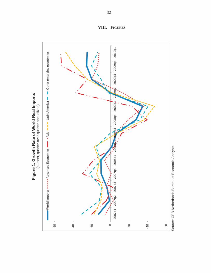
32

Figu

re 1

. Gro

wth

Rat

e of

Wor

ld R

eal I

mpo

rts

(per

cent

, qua

rter-o

ver-q

uarte

r ann

ualiz

ed)

S

ourc

e: C

PB

Net

herla

nds

Bur

eau

of E

cono

mic

Ana

lysi

s.

-60

-40

-200204060

2007

q120

07q2

2007

q320

07q4

2008

q120

08q2

2008

q320

08q4

2009

q120

09q2

2009

q320

09q4

2010

q1

Wor

ld im

port

sA

dvan

ced

Econ

omie

sA

sia

Latin

Am

eric

aO

ther

em

ergi

ng e

cono

mie

s

VIII. FIGURES

33

Fi

gure

2. E

volu

tion

of Im

port

s in

Cris

is a

nd N

on-C

risis

Cou

ntrie

s

Not

e: D

ashe

d lin

e sh

ows

a lin

ear p

recr

isis

tren

d, b

ased

on

2001

-200

7 pe

riod.

S

ourc

e: IM

F D

irect

ion

of T

rade

Sta

tistic

s.

4.2

4.3

4.4

4.5

4.6

4.7

4.8

4.95

2006

q120

07q1

2008

q120

09q1

2010

q1

Real

Impo

rts

of N

oncr

isis

Cou

ntri

es (i

n lo

gs)

4.2

4.3

4.4

4.5

4.6

4.7

4.8

4.95

2006

q120

07q1

2008

q120

09q1

2010

q1

Real

Impo

rts

of C

risi

s Co

untr

ies

(in

logs

)

34

Figure 3. Distribution of Crises across Time and Regions

0

2

4

6

8

10

12

14

1970

1972

1974

1976

1978

1980

1982

1984

1986

1988

1990

1992

1994

1996

1998

2000

2002

2004

2006

2008

Banking Crises Advanced economies Asia

Latin America Central and Eastern Europe and CIS

Africa Middle East

0

2

4

6

8

10

12

1970

1972

1974

1976

1978

1980

1982

1984

1986

1988

1990

1992

1994

1996

1998

2000

2002

2004

2006

2008

Debt Crises Advanced economies Asia

Latin America Central and Eastern Europe and CIS

Africa Middle East

35

Figure 4. Evolution of Imports and Exports Following Crises: A First Look

Notes: This figure shows the estimated coefficients from a regression of bilateral imports (in logs) on indicators of crisis in the exporter and importer, and ten lags of this indicator; the regression also includes exporter-importer pair dummies and year dummies. "t" , "t+1", "t+2" etc. represents the evolution of trade in "t", "t+1", "t+2" etc. following a crisis in year "t". The dotted lines show the 90% confidence interval around the estimated coefficients.

-0.35

-0.25

-0.15

-0.05

0.05t-1 t t+1 t+2 t+3 t+4 t+5 t+6 t+7 t+8 t+9 t+10

Imports

-0.35

-0.25

-0.15

-0.05

0.05

t-1 t t+1 t+2 t+3 t+4 t+5 t+6 t+7 t+8 t+9 t+10

Exports

36

Figure 5. Evolution of Imports and Exports Following Crises: Gravity Model

Notes: This figure shows the estimated coefficients from the fully specified gravity model in Equation (1) and Table 2. "t" , "t+1", "t+2" etc. represents the evolution of trade in "t", "t+1", "t+2" etc. following a crisis in year "t". The dotted lines show the 90% confidence interval around the estimated coefficients.

-0.25

-0.15

-0.05

0.05

t-1 t t+1 t+2 t+3 t+4 t+5 t+6 t+7 t+8 t+9 t+10

Imports

-0.25

-0.15

-0.05

0.05

t-1 t t+1 t+2 t+3 t+4 t+5 t+6 t+7 t+8 t+9 t+10

Exports

37

Figure 6a. Evolution of Exchange Rates Following Crises

Notes: The chart plots the coefficients from a regression of the exchange rate (local currency per US dollar) (in logs) on crisis and ten lags, country and year fixed effects. "t" , "t+1", "t+2" etc. represents the evolution of the exchange rate in "t", "t+1", "t+2" etc. following a crisis in year "t". The dotted lines show the 90% confidence interval around the estimated coefficients.

-1.20

-1.00

-0.80

-0.60

-0.40

-0.20

0.00

0.20

0.40

0.60t-1 t t+1 t+2 t+3 t+4 t+5 t+6 t+7 t+8 t+9 t+10

38

Figu

re 6

b. W

hy a

Per

sist

ent D

rop

in Im

port

s Fo

llow

ing

Cris

es?

Not

es. E

ach

char

t plo

ts th

e co

effic

ient

s fro

m a

regr

essi

on o

f the

var

iabl

e st

ated

on

top

of th

e ch

art (

in lo

gs) o

n cr

isis

and

ten

lags

, cou

ntry

and

yea

r fix

ed e

ffect

s. "t

" , "t

+1",

"t+2"

etc

. rep

rese

nts

the

evol

utio

n of

the

cha

nnel

in "t

", "t+

1", "

t+2"

etc

. fol

low

ing

a cr

isis

in y

ear "

t". T

he d

otte

d lin

es s

how

th

e 90

% c

onfid

ence

inte

rval

aro

und

the

estim

ated

coe

ffici

ents

.

-0.2

-0.1

5

-0.1

-0.0

50

0.050.

1t-

1t

t+1

t+2

t+3

t+4

t+5

t+6

t+7

t+8

t+9

t+10

Num

ber o

f Im

port

ed V

arie

ties

-0.0

3

-0.0

2

-0.0

10

0.01

0.02

0.03

t-1

tt+

1t+

2t+

3t+

4t+

5t+

6t+

7t+

8t+

9t+

10

Num

ber

of T

rade

Pro

tect

ion

Mea

sure

s

-0.1

-0.0

50

0.050.

1

0.15

Tari

ffs

-0.6

-0.4

-0.20

0.2

0.4

0.6

0.8

t-1

tt+

1t+

2t+

3t+

4t+

5t+

6t+

7t+

8t+

9t+

10

Vola

tility

of E

xcha

nge

Rate

39

Figure 7. Evolution of Imports and Exports Following Crises: Robustness

Notes: This figure shows the coefficient estimates of crisis dummies from various robustness tests conducted in Table 4. "t" , "t+1", "t+2" etc. represents the evolution of trade in "t", "t+1", "t+2" etc. following a crisis in year "t".

-0.25

-0.15

-0.05

0.05

t-1 t t+1 t+2 t+3 t+4 t+5 t+6 t+7 t+8 t+9

Imports

Baseline Country-Pair ControlsHMR Cyclical/TrendElasticity Crisis Aggregate DemandExchange rate and prices No current crisisvary multilateral resistance Aggregate

-0.25

-0.15

-0.05

0.05

t-1 t t+1 t+2 t+3 t+4 t+5 t+6 t+7 t+8 t+9

Exports

40

Figure 8. Evolution of Imports and Exports Following Crises: Robustness

Notes. This figure shows the coefficient estimates of crisis dummies from various robustness tests conducted in Table 5. "t" , "t+1", "t+2" etc. represents the evolution of trade in "t", "t+1", "t+2" etc. following a crisis in year "t".

-0.25

-0.2

-0.15

-0.1

-0.05

0t-1 t t+1 t+2 t+3 t+4 t+5 t+6 t+7 t+8 t+9 t+10

Imports

Baseline No contemporaneous crisis

Include lagged output Include lagged trade

-0.25

-0.2

-0.15

-0.1

-0.05

0

0.05

t-1 t t+1 t+2 t+3 t+4 t+5 t+6 t+7 t+8 t+9 t+10

Exports

Baseline

No contemporaneous crisis

Include lagged output

Include lagged trade

41

Figure 9. Evolution of Imports and Exports for Different Product Categories Notes: This figure shows the coefficient estimates of crisis dummies from the fully specified product-level gravity model in Equation (3). "t" , "t+1", "t+2" etc. represents the evolution of trade in "t", "t+1", "t+2" etc. following a crisis in year "t". The classification into product groups follows Pula and Peltonen (2009), see text for details.

-0.24

-0.19

-0.14

-0.09

-0.04

0.01

0.06

0.11

0.16

t-1 t t+1 t+2 t+3 t+4 t+5 t+6 t+7 t+8 t+9 t+10

Exports

Consumer Non Durables Intermediates Durables Primary

-0.24

-0.19

-0.14

-0.09

-0.04

0.01

0.06

0.11

0.16

t-1 t t+1 t+2 t+3 t+4 t+5 t+6 t+7 t+8 t+9 t+10

Imports

Consumer Non Durables Intermediates Durables Primary

42

Figu

re 1

0. E

volu

tion

of Im

port

s an

d Ex

port

s Fo

llow

ing

Cris

es d

urin

g G

loba

l Dow

ntur

ns

Not

es. T

his

figur

e sh

ows

the

coef

ficie

nt e

stim

ates

of c

risis

dum

mie

s fro

m th

e fu

lly s

peci

fied

grav

ity m

odel

in E

quat

ion

(4),

allo

win

g th

e co

effic

ient

s on

cris

is d

umm

ies

to v

ary

in y

ears

of g

loba

l dow

ntur

n. T

he y

ears

of g

loba

l dow

ntur

n ar

e 19

75, 1

982,

199

1, 2

001

and

2008

. "t"

, "t+

1", "

t+2"

etc

. re

pres

ents

the

evol

utio

n of

trad

e in

"t",

"t+1"

, "t+

2" e

tc. f

ollo

win

g a

cris

is in

yea

r "t".

The

dot

ted

lines

sho

w th

e 90

% c

onfid

ence

inte

rval

aro

und

the

estim

ated

coe

ffici

ents

.

-0.4

-0.3

5

-0.3

-0.2

5

-0.2

-0.1

5

-0.1

-0.0

50t-

1t

t+1

t+2

t+3

t+4

t+5

t+6

t+7

t+8

t+9

t+10

Impo

rts

-Glo

bal D

ownt

urn

-0.4

-0.3

5

-0.3

-0.2

5

-0.2

-0.1

5

-0.1

-0.0

50t-

1t

t+1

t+2

t+3

t+4

t+5

t+6

t+7

t+8

t+9

t+10

Impo

rts

-No

Glo

bal D

ownt

urn

-0.4

-0.3

-0.2

-0.10

0.1

0.2

t-1

tt+

1t+

2t+

3t+

4t+

5t+

6t+

7t+

8t+

9t+

10

Expo

rts

-No

Glo

bal D

ownt

urn

-0.4

-0.3

-0.2

-0.10

0.1

0.2

t-1

tt+

1t+

2t+

3t+

4t+

5t+

6t+

7t+

8t+

9t+

10

Expo

rts

-Glo

bal D

ownt

urn

43

Figure 11. Evolution of Imports and Exports Following Crises in Importer and Exporter

Notes: This figure shows the coefficients estimates of crisis dummies from the fully specified gravity model in Equation (5), including an additional dummy for crisis in both importer and exporter. The coefficients on the right panel are calculated by summing up the coefficients on crisis in importer, crisis in exporter and crisis in both. "t" , "t+1", "t+2" etc. represents the evolution of trade in "t", "t+1", "t+2" etc. following a crisis in year "t". The dotted lines show the 90% confidence interval around the estimated coefficients.

-0.5

-0.4

-0.3

-0.2

-0.1

0

0.1t-1 t t+1 t+2 t+3 t+4 t+5 t+6 t+7 t+8 t+9 t+10

Imports - crisis in importer and exporter

44

Figu

re 1

2. E

volu

tion

of Im

port

s an

d Ex

port

s Fo

llow

ing

Cris

es: P

re a

nd P

ost-

1990

Not

es. T

his

figur

e sh

ows

the

coef

ficie

nts

estim

ates

of c

risis

dum

mie

s fro

m th

e fu

lly s

peci

fied

grav

ity m

odel

in E

quat

ion

(1),

allo

win

g th

e co

effic

ient

s on

cris

is d

umm

ies

to v

ary

befo

re a

nd a

fter 1

990.

"t" ,

"t+1

", "t+

2" e

tc. r

epre

sent

s th

e ev

olut

ion

of tr

ade

in "t

", "t+

1", "

t+2"

etc

. fol

low

ing

a cr

isis

in y

ear "

t". T

he d

otte

d lin

es s

how

the

90%

con

fiden

ce in

terv

al a

roun

d th

e es

timat

ed c

oeffi

cien

ts.

-0.4

-0.3

-0.2

-0.10

t-1

tt+

1t+

2t+

3t+

4t+

5t+

6t+

7t+

8t+

9t+

10

Impo

rts

-Pre

199

0

-0.4

-0.3

5-0

.3-0

.25

-0.2

-0.1

5-0

.1-0

.050

0.05

t-1

tt+

1t+

2t+

3t+

4t+

5t+

6t+

7t+

8t+

9t+

10

Impo

rts

-Pos

t 199

0

-0.1

-0.0

50

0.050.

1

0.150.

2t-

1t

t+1

t+2

t+3

t+4

t+5

t+6

t+7

t+8

t+9

t+10

Expo

rts

-Pre

199

0

-0.1

-0.0

50

0.050.

1

0.150.

2t-

1t

t+1

t+2

t+3

t+4

t+5

t+6

t+7

t+8

t+9

t+10

Expo

rts

-Pos

t 199

0

45

IX. REFERE CES

Altomonte, Carlo, and Gianmarco I.P. Ottaviano, 2009, “Resilient to the Crisis? Global Supply Chains and Trade Flows,” in The Great Trade Collapse: Causes, Consequences and Prospects, ed. by Richard Baldwin. Available at www.voxeu.org/index.php?q=node/4289.

Anderson, James, and Eric Van Wincoop, 2003, “Gravity with Gravitas: A Solution to the Border Puzzle,” American Economic Review, Vol. 93, No. 1, pp. 170–92.

Bai, Jushan, and Serena Ng, 2004, “A PANIC Attack on Unit Roots and Cointegration,” Econometrica, Vol. 72, pp. 1127-77.

Baldwin, Richard, 1988, “Hysteresis in Import Prices: The Beachhead Effect,” American Economic Review, Vol. 78, No. 4, pp. 773–85.

Baldwin, Richard, ed., 2009, The Great Trade Collapse: Causes, Consequences and Prospects. Available at www.voxeu.org/index.php?q=node/4297.

———, and Daria Taglioni, 2006, “Gravity for Dummies and Dummies for Gravity Equations,” NBER Working Paper No. 12516 (Cambridge, Massachusetts: National Bureau of Economic Research).

Bems, Rudolphs, Robert C. Johnson and Kei-Mu Yi, 2010, “Demand Spillovers and the Collapse of Trade in the Global Recession,” IMF Economic Review, forthcoming.

Beim, David and Charles Calomiris, 2001, Emerging Financial Markets. Appendix to Chapter (New York: McGraw-Hill/Irwin Publishers).

Berman, Nicolas, and Philippe Martin, 2010, “The Vulnerability of Sub-Saharan Africa to the Financial Crisis: The Case of Trade,” CEPR Discussion Paper No. 7765 (London: Centre for Economic Policy Research).

Bernard, Andrew, J. Bradford Jensen, Stephen J. Redding, and Peter K. Schott, 2009, “The Margins of U.S. Trade,” American Economic Review, Vol. 99, No. 2, pp. 487–93.

Blomberg, S. Brock and Gregory D. Hess, 2006, “How Much Does Violence Tax Trade?, ” The Review of Economics and Statistics, vol. 88(4), pages 599-612, October.

Bown, Chad P. (2010) “Global Antidumping Database,” available at http://econ.worldbank.org/ttbd/gad/.

Braun, Matías and Borja Larrain, 2005, “Finance and the Business Cycle: International, Inter-Industry Evidence,” Journal of Finance, Vol. 60, No. 3, pp. 1097-1128.

46

Caprio, Gerard, Daniela Klingebiel, Luc Laeven and Guillermo Noguera, 2005, “Appendix: Banking Crisis Database.” In Patrick Honohan and Luc Laeven (eds.). Systemic Financial Crises: Containment and Resolution (Cambridge, U.K.: Cambridge University Press).

Cerra, Valerie, and Sweta Saxena, 2008, “Growth Dynamics: The Myth of Economic Recovery,” American Economic Review, Vol. 98, No. 1, pp. 439–57.

Cook, David and Michael Devereux, 2006, “External Currency Pricing and the East Asian Crisis,” Journal of International Economics, Vol. 69, No. 1, pp 37-63.

Eaton, Jonathan, Sam Kortum, Brent Neiman, and John Romalis, 2010, “Trade and the Global Recession” (unpublished; Chicago, Illinois: University of Chicago).

Feenstra, Robert, 2002, Advanced International Trade: Theory and Evidence (Princeton University Press).

Feenstra, Robert, Robert Lipsey, Haiyan Deng, Alyson Ma, and Hengyong Mo, 2005, “World Trade Flows: 1962–2000,” NBER Working Paper No. 11040 (Cambridge, Massachusetts: National Bureau of Economic Research).

Frankel, Jeffrey, Ernesto Stein, and Shang-Jin Wei, 1996, “Regional Trading Arrangements: Natural or Supernatural?” American Economic Review, Vol. 86, No. 2, pp. 52–56.

Freund, Caroline, 2009, “The Trade Response to Global Downturns: Historical Evidence,” Policy Research Working Paper No. 5015 (Washington: World Bank).

Friedman, Jed, and James Levinsohn, 2003, “The Distributional Impact of Indoensia’s Financial Crisis on Household Welfare: A Rapid Response Methodology,” The World Bank Economic Review, Vol. 16, No. 3, pp. 397-423.

Glick, Reuven, and Andrew K. Rose, 2002, “Does a Currency Union Affect Trade? The Time Series Evidence,” European Economic Review, Vol. 46, No. 6, pp. 1125–51.

Glick, Reuven, and Alan M. Taylor, 2010, “Collateral Damage: Trade Disruption and the Economic Impact of War,” The Review of Economics and Statistics, Vol. 92, No. 1, pp. 102–27.

Gregory, Rob, Christian Henn, Brad McDonald and Mika Saito, 2010, “Trade and the Crisis: Protect or Recover,” IMF Staff Position Note 10/07 (Washington: International Monetary Fund).

Harrigan, James, 2003 “Specialization and the Volume of Trade: Do the Data Obey the Laws?” chapter in The Handbook of International Trade, Basil Blackwell, edited by

47

James Harrigan and Kwan Choi. Also available as NBER Working Paper No. 8675 and Federal Reserve Bank of ew York Staff Report No. 140.

Harrigan, James, 1996, “Openness to Trade in Manufactures in the OECD,” The Journal of International Economics, v. 40 nos. 1/2 (February): 23-39.

Helpman, Elhanan, Marc Melitz and Yona Rubinstein, 2008. “Estimating Trade Flows: Trading Partners and Trading Volumes,” The Quarterly Journal of Economics, MIT Press, vol. 123(2), pages 441-487.

Im, Kyung So, M. Hashem Pesaran, and Yongcheol Shin, 2003, “Testing for Unit Roots in Heterogeneous Panels,” Journal of Econometrics, Vol. 115, pp. 53-74.

International Monetary Fund (IMF), 2004, “A New Look at Exchange Rate Volatility and Trade Flows,” IMF Occasional Paper No. 235 (Washington: International Monetary Fund).

International Monetary Fund (IMF), 2008, “Structural Reforms and Economic Performance in Advanced and Developing Countries,” paper by the Research Department (Washington). Available at www.imf.org/external/np/res/docs/2008/0608.htm.

International Monetary Fund (IMF), 2009, “What’s the Damage? Medium-term Output Dynamics after Financial Crises,” World Economic Outlook, Chapter 4, October.

Judson, Ruth A. and Ann L. Owne, 1999, “Estimating Dynamic Panel Data Models: A Guide for Macroeconomists,” Economic Letters, 65(1): 9-15.

Kaminsky, Graciela, L., and Carmen M. Reinhart, 1999, “The Twin Crises: The Causes of Banking and Balance of Payments Problems,” American Economic Review, Vol. 89, No. 3, pp. 473–500.

Klein, Michael W. and Jay C. Shambaugh, 2006, “Fixed Exchange Rates and Trade,” Journal of International Economics, Vol. 70, pp. 359–83.

Laeven, Luc, and Fabian Valencia, 2008, “Systemic Banking Crises: A New Database,” IMF Working Paper 08/224 (Washington: International Monetary Fund).

Laeven, Luc, and Fabian Valencia, 2010, “Resolution of Banking Crises: The Good, the Bad, and the Ugly,” IMF Working Paper 10/146 (Washington: International Monetary Fund).

Levchenko, Andrei, Logan Lewis, and Linda Tesar, 2010, “The Collapse of International Trade during the 2008-2009 Crisis: In Search of the Smoking Gun,” IMF Economic Review, forthcoming.

48

Ma, Zihui and Leonard Cheng, 2003, “The Effects of Financial Crises on International Trade,” NBER Working Paper No. 10172 (Cambridge, Massachusetts: National Bureau of Economic Research).

Martin, Philippe, Thierry Mayer, and Mathias Thoenig, 2008, “Make Trade, Not War?” Review of Economic Studies, Vol. 75, No. 3, pp. 865–900.

Nickell, Stephen, J., 1981, “Biases in Dynamic Models with Fixed Effects,” Econometrica, 49(6): 1417-26.

O’Rourke, Kevin, 2009, “Government Policies and the Collapse in Trade during the Great Depression,” in The Great Trade Collapse: Causes, Consequences and Prospects, ed. by Richard Baldwin. Available at www.voxeu.org/index.php?q=node/4267.

Pesaran, M. Hashem, 2007, “A Simple Panel Unit Root Test in the Presence of Cross Section Dependence,” Journal of Applied Econometrics, Vol. 22, pp. 265-312.

Pedroni, Peter, and Y. Yao, 2006, “Regional Income Divergence in China,” Journal of Asian Economics, Vol. 17, pp. 294-315.

Pedroni, Peter, 2004, “Panel Cointegration; Asymptotic and Finite Sample Properties of Pooled Time Series Tests with an Application to the PPP Hypothesis,” Econometric Theory, Vol. 20, 597-625.

Pedroni, Peter, 2000, “Fully-Modified OLS for Heterogeneous Cointegrated Panels,” Advances in Econometrics, 15, 93-130, 2000.

Pedroni, Peter, 1999, “Critical Values for Cointegration Tests in Heterogeneous Panels with Multiple Regressors,” Oxford Bulletin of Economics and Statistics, Vol. 61, pp. 653-70.

Pula, Gabor, and Tuomas Peltonen, 2009, “Has Emerging Asia Decoupled? An Analysis of Production and Trade Linkages Using the Asian International Input-Output Table,” ECB Working Paper No. 993 (Frankfurt: European Central Bank).

Qureshi, Mahvash Saeed, 2009, “Trade and Thy Neighbor’s War,” IMF Working Paper 09/283 (Washington: International Monetary Fund).

Reinhart, Carmen, and Kenneth Rogoff, 2008, “Banking Crises: An Equal Opportunity Menace”, NBER Working Paper No. 14587 (Cambridge, Massachusetts: National Bureau of Economic Research).

Reinhart, Carmen, and Kenneth Rogoff, 2009a, This Time is Different: Eight Centuries of Financial Folly, Princeton University Press.

49

Reinhart, Carmen, and Kenneth Rogoff, 2009b, “The Aftermath of Financial Crises,” American Economic Review, Vol. 99, No. 2: 466-472.

Rose, Andrew, 2000, “One Money, One Market: Estimating the Effect of Common Currencies on Trade,” Economic Policy, Vol. 15, No. 30, pp.7–46.

Sturzenegger, Federico, and Jeromin Zettelmeyer, 2006, Debt Defaults and Lessons Decade of Crises, Table 1 in Chapter 1, (Cambridge: MIT Press).

Thursby, Marie, and Jerry Thursby, 1987, “Bilateral Trade Flows, the Linder Hypothesis, and Exchange Risk,” The Review of Economics and Statistics, Vol. 69, No. 3, pp.488–95.

World Bank, 2002. Global Development Finance, Appendix on Commercial Debt Restructuring (Washington: World Bank).

Yu, Miaojie, 2010, “Trade, Democracy and the Gravity Equation,” Journal of Development Economics, Vol. 91, pp.289–300.

50

X. APPE DICES

Appendix 1. Data Sources The primary data sources for the chapter are the IMF’s Direction of Trade Statistics (DOTS), World Economic Outlook (WEO) and International Financial Statistics (IFS) databases, the NBER-UN World Trade Flows database (2005), and Laeven and Valencia (2008, 2010). Additional data sources are listed in Table A3.

Crisis indicators are from Laeven and Valencia (2008, 2010). Laeven and Valencia (2010) present new and comprehensive data on the starting dates and characteristics of systemic banking crises over the period 1970-2009, building on earlier work by Caprio et al. (2005), Laeven and Valencia (2008), and Reinhart and Rogoff (2009a). They update the Laeven and Valencia (2008) database on systemic banking crises to include the recent episodes following the U.S. mortgage crisis of 2007, and identify 129 episodes since 1970.

Laeven and Valencia (2008) also identify debt crisis episodes based on sovereign debt default and restructuring by relying on information from Beim and Calomiris (2001), World Bank (2002), Sturzenegger and Zettelmeyer (2006), and IMF Staff reports. The information compiled includes the year of sovereign default to private lending and the year of debt rescheduling. Using this approach, they identify 60 episodes of sovereign debt defaults and restructurings since 1970.

Data on bilateral and aggregate imports and exports from the DOTS database are reported in current U.S. dollars. These are deflated using the world import and export price deflators, respectively, from the IFS database, to get each economy’s real imports and exports. The series on real GDP in U.S. dollars is from the WEO database. Import- and export-weighted partner GDP and GDP per capita are constructed using real GDP in U.S. dollars and import and export weights from the DOTS database. These weights vary each year based on the actual import and export flows between economies.

Data on imports and exports by product category are constructed from the NBER-UN World Trade Flows database (see Feenstra and others, 2005). The data base is first extended using the UN Comtrade database. The Standard International Trade Classification, Revision 2 (SITC Rev. 2) codes that identify products in the NBER-UN trade data are matched to the UN Broad Economic Classification (BEC) codes. These are then classified into Capital Goods, Consumer Durables, Consumer Non Durables, Intermediate Goods and Primary Goods, following Pula and Peltonen (2009).

The measure of trade liberalization is from the IMF Structural Reforms Database and is described in IMF (2008).

51

Appendix 2. Time-series properties of imports and GDP

In order to examine the time-series properties of the two key variables—real imports and real GDP—we use recently developed techniques for analyzing non-stationary macro panel data. The tests are very general in that they allow for country fixed effects, heterogeneous trends, and common time effects. First we test for the presence of unit roots using three tests: (i) the Im, Pesaran and Shin augmented Dickey-Fuller test, adjusted for small sample size distortions using bootstrapping techniques (Im, Pesaran, and Shin, 2003, and Pedroni and Yao, 2006); (ii) the Bai and Ng (2004) test; and (iii) the Pesaran (2007) cross-sectionally augmented Dickey-Fuller (CADF) test. Tests (ii) and (iii) take into account common factor dependencies in a panel, a more general form of cross-sectional dependency than allowed for by the use of time-effects. The results reported in Table A2 show that most of the tests fail to reject the null of unit root in both real imports and real GDP. Next, we also conduct tests of cointegration between real imports and real GDP as suggested by Pedroni (2004) and Pedroni (1999). The tests treat all parameters as heterogeneous across members of the panel, and allow for both heterogeneous dynamics and heterogeneous cointegrating vectors, as well as complete endogeneity. The bottom panel of Table A2 shows four commonly used test statistics: (i) pooled Phillips-Perron t-statistics, (ii) pooled ADF t-statistics, (iii) group-mean Phillips Perron t-statistics and (iv) group mean ADF t-statistics. All four test statistics reject the null of no cointegration. Given the evidence for cointegration, we estimate the empirical specification in levels. Under cointegration, standard panel techniques produce superconsistent estimates of slope coefficients (the rate of convergence is faster in the panel than even the time series case); we get precise estimates even in small panels and even if regressors are endogenous.

52

XI. APPE DIX TABLES

Table A1. Summary Statistics to Main Variables

Variable Nobs Mean StDev Min MaxCrisis in Importer 372060 0.034 0.182 0 1Crisis in Exporter 372060 0.034 0.182 0 1Log Trade 372060 1.009 3.736 -32.898 12.255Log Importer GDP 372060 3.450 2.160 -2.800 9.376Log Exporter GDP 372060 3.564 2.112 -2.800 9.376Log Importer GDP Per Capita 372060 -12.871 1.642 -16.315 -9.776Log Exporter GDP Per Capita 372060 -12.819 1.636 -16.315 -9.776Log Distance 291764 4.071 0.826 0.297 5.6611 if Common Border 291764 0.029 0.168 0 11 if Island 372060 0.010 0.101 0 11 if Landlock 372060 0.011 0.102 0 11 if Common Legal System 291764 0.359 0.480 0 11 if Common Language 291764 0.303 0.460 0 11 if Colonial Times 291764 0.018 0.134 0 11 if Currency Union 372060 0.014 0.116 0 11 if Free Trade Area 372060 0.048 0.214 0 1

53

Tabl

e A

2. P

anel

Uni

t Roo

t and

Coi

nteg

ratio

n Te

sts

Ln

(im

ports

)

Ln (r

eal G

DP

)

1 %

cr

itica

l va

lues

5%

criti

cal

valu

es

Uni

t Roo

t Tes

ts (N

ull=

Uni

t Roo

t, La

rge

nega

tive

valu

es im

ply

reje

ctio

n)

Boo

tstra

pped

Im, P

esar

an &

Shi

n A

DF

stat

istic

0.

10

0.19

-1

.28

-1.6

4 B

ai-N

g (2

004)

with

orth

ogon

aliz

ed d

ata

Im, P

esar

an &

Shi

n A

DF

stat

istic

5.

73

-1.8

6 -1

.28

-1.6

4

Pes

hara

n (2

007)

cro

ss-s

ectio

nally

aug

men

ted

AD

F st

atis

tic

-2.2

6 -2

.12

-5.0

1 -4

.01

Coi

nteg

ratio

n Te

sts

(Nul

l=N

o C

oint

egra

tion,

Lar

ge n

egat

ive

valu

es im

ply

reje

ctio

n)

Poo

led

Phi

llips-

Per

ron

stat

istic

-5

.98

-1.2

8 -1

.64

Poo

led

AD

F st

atis

tic

-1.9

3 -1

.28

-1.6

4 G

roup

mea

n P

hillip

s-P

erro

n st

atis

tic

-7.6

0 -1

.28

-1.6

4 G

roup

mea

n A

DF

stat

istic

-3

.84

-1.2

8 -1

.64

Num

ber o

f cou

ntrie

s 17

9 17

9

Num

ber o

f per

iods

40

40

Not

es. W

e dr

op c

ount

ries

with

less

than

10

year

s of

dat

a. A

ll re

porte

d te

st s

tatis

tics

(exc

ept f

or P

esha

ran

(200

7) te

st s

tatit

ic) a

re d

istri

bute

d N

(0,1

) un

der n

ull o

f uni

t roo

t or n

o co

inte

grat

ion)

. The

repo

rted

valu

es o

f tes

t sta

tistic

s sh

own

in th

e ta

ble

are

calc

ulat

ed a

ssum

ing

3 la

gs. T

he v

alue

s ar

e si

mila

r if w

e us

e 4,

5 o

r 6 la

gs.

54

Table A3. Data Sources

Annual Data Variable Source

Real Exports and Imports Direction of Trade Statistics (DOTS) Database Real GDP in U.S. Dollars World Economic Outlook (WEO) Database Real GDP per Capita in U.S. Dollars WEO Database World Import/Export Price Deflator International Financial Statistics (IFS) Database Bilateral exchange rate IMF Real Effective Exchange Rate IMF Product-Level Imports and Exports Feenstra and others (2005), COMTRADE, Pula and

Peltonen (2009) Trade Liberalization IMF Debt Crisis Indicators Laeven and Valencia (2008) Banking Crisis Indicators Laeven and Valencia (2010) High-Frequency Data

Variable Source Real Exports and Imports CPB Netherlands Bureau of Economic Policy

Analysis, DOTS Database, Global Trade Atlas, Haver Analytics

Antidumping Data Bown (2010) World Import/Export Price Deflator IFS Database, CPB Netherlands Bureau of

Economic Policy Analysis