how does fiscal policy affect monetary policy in the ... · regime may also arise when fiscal...
TRANSCRIPT
Munich Personal RePEc Archive
How does fiscal policy affect monetarypolicy in the Southern AfricanCommunity (SADC)?
Obinyeluaku, Moses and Viegi, Nicola
National Treasury South Africa, University of Cape Town
25 May 2009
Online at https://mpra.ub.uni-muenchen.de/15372/
MPRA Paper No. 15372, posted 25 May 2009 09:30 UTC

1
How Does Fiscal Policy Affect Monetary Policy
in Southern African Development Community
(SADC)?
Moses Obinyeluaku1
National Treasury South Africa and University of Cape Town
Nicola Viegi2
University of Cape Town and ERSA
May 2009
Abstract
Fiscal policy can affect monetary policy either through debt monetisation or through a direct
effect on price dynamics. The former is the conventional classical view rooted in the quantity
theory of money while the latter is the modern view of the Fiscal Theory of Price
Determination. Based on the dynamic response of inflation to different shocks, we test the
relationship between fiscal balances and monetary stability in 10 SADC countries. Results
show that five out of 10 countries considered here were characterised throughout the period
1980-2006 by fiscally dominant regimes, with weak or no response of primary surpluses to
public liabilities. The remaining five countries exhibit a monetary dominant regime. The
study also finds that changes in primary surpluses affect price variability via aggregate
demand, suggesting that fiscal outcomes could be a direct source of inflation variability, hence,
the need for policy coordination in the region.
Keywords: African Economic Integration, Fiscal Monetary Policy Coordination, VAR
Analysis.
JEL Classification Numbers: E63, F15, C32
1 [email protected] : I wish to acknowledge financial support by CODESRIA during the preparation of this
paper 2 [email protected]

2
I. INTRODUCTION
Understanding the nature of the relationship between monetary and fiscal policy is central in
the process of designing institution for macroeconomic stability and growth. In the debate
about the process of African integration the issue of the correct policy framework that each
country should follow is an important part of the policy discussion.
The main preoccupation of policy makers is that undisciplined fiscal policies could jeopardize
monetary stability for the whole Southern Africa. In a “fiscal dominant” regime, where the
fiscal authority sets the budget independently of public sector liabilities; a fiscal expansion
may eventually require monetization, and result in higher inflation. However money creation
may not be the only channel through which fiscal policy becomes dominant. Fiscal dominant
regime may also arise when fiscal policy is not sustainable and government bonds are
considered net wealth.3 The implication is that fiscal policy can be the main determinant of
inflation.
This paper tests the nature of fiscal and monetary policy interdependence in SADC. The main
objective is to investigate whether fiscal policy is dominating monetary policy and whether
fiscal instability contributes directly to the price dynamics.
The paper is organised as follows. In the next section we review some of the debate about
fiscal and monetary policy interdependence, with a particular attention paid to the so called
Fiscal Theory of Price Determination (FTPD). In the second part, using data for the period
1980-2006 for 10 Southern African countries, we investigate whether some of the implications
of the FTPD are indeed a feature of the SADC region. The last section concludes.
II. THE INTERTEMPORAL APPROACH TO FISCAL AND MONETARY POLICY
INTERDEPENDENCE
Modern analysis of interdependence between monetary and fiscal policy has a central point of
reference in the seminal paper by Sargent and Wallace (1981) “Unpleasant Monetarist
Arithmetic”. The main objective of the paper was to show that, even in a pure monetarist
framework, unbounded fiscal policy produces negative spillover effects on monetary policy,
and ultimately it can undermine the ability of monetary policy to control inflation.
This conclusion largely based on the “assumption” that permanent budget deficits must be
eventually monetized. Not surprisingly, with an exogenous stream of budget deficits, there is
only one integral of money creation that is consistent with long run equilibrium (in term of 3 See Woodford (1998).

3
satisfaction of agents trasversality conditions), and the only choice in the hand of the monetary
authority is the time profile of money creation.
In the words of Sargent and Wallace: "Without help from the fiscal authorities, fighting current
inflation with tight monetary policy must eventually lead to higher future inflation”.
On the other hand, the introduction of rational expectations has the effect of anticipating the
inflationary pressure at time zero. This eliminates even the possibility of choosing the desired
time profile of inflation consistent with the long run solvency of the public sector.
But the most influential result of the Sargent and Wallace contribution has probably been the
fact that the policy conflict between fiscal and monetary policy could be resolved simply by
assigning policy leadership to the Central Bank. If it was possible to give the "first move" to
the monetary authority, then the fiscal authority would be constrained in its policy choice by
the amount of seignorage provided by the Central Bank.
In fact, in the Sargent and Wallace model, the monetary authority is the loser of the policy
game simply because is not able to influence the spending decision of the fiscal authority.
Sargent and Wallace themselves recognise that the conflict could be resolved with appropriate
institutional arrangements. As they say "One can imagine a monetary authority sufficiently
powerful vis-à-vis the fiscal authority that by the imposition of a slower rates of growth of base
money, both now and into indefinite future, it can successfully constrain fiscal policy by telling
the fiscal authority how much seignorage it can expect now and in the future".
A recent stream of research (Woodford 1995,1996 Sims,1993,1995, and Bergin, 1997a,
1997b), building on previous works of Calvo (1990) and Leeper (1991) among others, has
renovated the interest in the analysis of the interrelation between monetary and fiscal policy,
partly questioning the conclusions derived from the Sargent and Wallace approach. The main
innovation introduced by these contributions is that the interrelation between fiscal policy on
one side, and monetary policy and the private sector on the other, manifests itself through
changes in the level of prices that moves to achieve public sector solvency, independently of
the institutional arrangements between fiscal and monetary authority.
Variables like net government liabilities and expectations regarding the stream of future
surpluses are given an immediate role in the determination of the equilibrium price level. If the
government's solvency condition were not satisfied at a particular point in time, (i.e. the stream
of current and expected future surpluses would not pay the existing debt) price will move to
ensure that it does hold.

4
The first goal of this approach to monetary and fiscal policy interdependence is to derive
conditions under which the level of price is determined even in a regime of nominal short run
interest rate targeting. In the quantity theory tradition, when the monetary authority targets the
nominal interest rate, it supplies any amount of money demanded by the private sector. Given
that the demand of money is a demand for real money balances, a given quantity of real money
can be determined by an infinite number of combinations of nominal money supply and prices,
producing indeterminate levels of prices and money stocks (Patinkin, 1961, Sargent and
Wallace, 1975). On the contrary, the fiscal theory of price determination (FTPD) finds an
anchor for the price level in the dynamics of expected future fiscal surpluses.
The basic mechanism behind the theory can be illustrated using an infinite horizon model with
money in the utility function similar to the one used by Bergin(1997).In this model, a
representative agent solves a standard optimisation problem,
��
���
����
�
�+=
∞
=−
0
1,
loglog)(maxt t
t
t
t
tMB P
MCECU µβ (1)
subject to
( ) tt
t
t
t
t
t
t
t
t
t
t YP
M
P
Bi
P
M
P
BC τ−+++=++ −−
−11
11 (2)
and
0≥tB 0≥tM 0≥tC
where all the variables have the standard meaning, it is the nominal interest rate, the income Yt
is an independent and normally distributed positive random variables and τ is a lump sum tax
imposed by the government. The government budget constraint, expressed in nominal term, is:
( ) ( )1111 −−− −−+=+ ttttttt MMBiPB τ (3)
The government must fix two of the five variables in (3), or define a function for each of them,
in order for the model to be complete. The other three variables will then be determined by the
private agent first order conditions. The F.O.C are given by:
:C
U
δ
δ t
tCλ=
1 (4)
:B
U
δ
δ ( )
11
1
11
1
++
−+=tt
t
tt CPEi
CPβ (5)

5
:M
U
δ
δ
t
t
t
t
t Ci
i
P
M +=
1µ (6)
Suppose that the government follows a policy of nominal interest rate targeting and fixes i and
the level of taxes. Then the government budget constraint divided by PtCt is given by:
( )ttt
t
tt
t
tt
t
tt
tt
tt
t
CCP
M
CP
M
CP
Bi
CP
CP
CP
B τ−−��
�
�
�++=
−−
−
−−
−−−
11
1
11
111 1 (7)
Taking the expectations of (7) and using the private sector FOCs and the fact that in
equilibrium is C=Y, we have (using condition 5 and 6):
( ) ��
���
� −−−−=��
�
�
� −−
−−
−−− −
i
iYE
YP
B
YP
BE tt
tt
t
tt
t
tβ
ββµτβ
11
1
11
11
1 1 (8)
Equation (8) is an unstable difference equation (β<1), with the last term representing the
expected constant seignorage revenues, given the policy pegging nominal interest rate.
Condition (8) has a single stable solution, as:
( )[ ]µξτβ
β+
−= −
−1
11
tt YEPY
B (9)
where ξ is the constant term in equation (8). Given the level of taxes and the nominal interest
rate, (9) is the only value of real debt compatible with the solvency of the public sector.
Implicitly (9) represents the net present value of expected future surpluses, therefore any
movement in the present income, or taxes or interest rate will produce a movement in prices
such that the intertemporal budget constraint of the public sector is satisfied. Substituting this
equilibrium value of future surpluses, called Φ, in (7) it is possible to express the movement in
prices respect the other real variable in the model:
( )( )µξτ ++Φ
Φ+= −
− t
tt
t
t
Y
Yi
P
P 1
1
1 (10)
Equation (10) shows the relation between income and price dynamics when the government
follows an exogenous fiscal policy as the one studied by Sargent and Wallace.
This negative correlation between movements in prices and movement in real income is
determined only by the particular fiscal policy followed by the Government. A level of income
greater then its trend value eases the pressure on the level of prices coming from the fiscal side,
therefore reducing the level of prices itself. On the other hand the fiscal authorities can

6
influence the level of prices via changes in the tax rate with a result that is observationally
equivalent to the traditional demand effects of fiscal policy of the Keynesian tradition. A
reduction in taxes increases the wealth effect of the debt outstanding, thus increasing private
demand and prices until the real value of debt has not came back at its sustainable value.
The mechanism behind this relation totally depends on the wealth effect of public debt. In what
is this approach differ from the traditional way to describe the determination of fiscal policy
effects in a General Equilibrium Model? In building up a general equilibrium model similar to
the one described above, it is usual practice to close the model with two trasversality
conditions, one for each agent. On one hand a rational private agent is required to plan is
consumption-leisure choice in such a way that in the limit he will use all his available
resources:
( ) ( )[ ]��
���
��
���
−��
�
�
++++=
��
���
��
���
��
�
�
+
−∞
=
−∞
=
ss
ts
ts
t
t
t
t
t
s
ts
ts
t Yr
EP
M
P
BrC
rE τ
1
11
1
1
On the other hand the same condition is also imposed on the behaviour of the government
derived by integrating forward with a condition like (3), and imposing the final condition
01
1lim =�
�
�
�
+ +
+
+
∞→it
it
it
i P
B
r or
( ) ∞
=+
−+
��
�
�
+=
0
1
1
1
i
it
it
tr
D τ (11)
where D is the real value of debt issued by the government. As argued by Buiter (1998) "These
decision rules determine, jointly with the market clearing conditions, initial conditions and
other system wide constraints, the equilibrium sequences of prices. The Budget constraints
must be satisfied, however, both for equilibrium and for out of equilibrium sequences of
endogenous variables in order for these budget constraints to co-determine these equilibrium
sequences" (pp17-18). But in doing so, the equilibrium is imposed "ex ante", as a condition for
the formulation of the model itself, and it is not the result, ex post, of possible disequilibrium
dynamics.
In the FTPD instead, because the actual fiscal policy is expressed in nominal terms but the
trasversality condition (11) is expressed in real terms, it is possible that a disequilibrium
behaviour of the government produces a movement in prices that generates a new equilibrium
in which (11) is satisfied at an higher nominal debt and an higher level of prices. Only a policy

7
that explicitly follows a Ricardian rule, as defined by (11), produces total independence of
prices from fiscal dynamics.
For example, consider the case of a government following a tax policy that adjusts the level of
taxes to the level of real debt, as:
t
t
tP
B10 θθτ +−= (12)
Substituting this policy rule in the budget constraint (8) we obtain:
( ) ( )[ ]1
1
111
1
10
11
11
1 1 −−
−−−
−
−−
−−− −−��
�
�
�−+=��
�
�
�− ttt
tt
t
tt
tt
t
tt
t
t YYEYP
BEYE
YP
B
YP
BE t βµθθβ
or, simplifying:
( )[ ] ( )( ) ( )[ ]{ }1
1
1
1
10
111
1
1
1 1
1
1
1
1−
−−
−−
−−
−− −−
++
+=��
�
�
�− tttt
tt
t
tt
t
t YYEYEYP
B
YP
BE t βµθ
θβθ (13)
that is a stable difference equation as long as (1+θ1)β is greater than 1. The meaning of
equation (13) is pretty obvious: if taxes react to the increase in debt strongly enough, equation
(13) is stable and a policy of pegging the level of prices does not conflict with the equilibrium
of the public sector4.
It is clear that the above approach greatly reduces the role of the monetary authorities in
determining the price level and, at the same time, casts serious doubt that the independence of
the central bank should be the sole instrument for price stability. As argued by Posen (1993),
Central Bank independence is not the instrument for achieving price stability by itself, but is
the way in which the fiscal authorities have signalled to the market their willingness to stabilise
the fiscal position, therefore achieving price stability through a change in fiscal stance. On the
other hand monetary policy independence cannot achieve price stability without a fiscal policy
coherent with that objective.
This possible characteristic of monetary and fiscal policy interaction matters when thinking at
process of economic integration and monetary cooperation. The possibility to delegate
monetary policy to an independent and supranational institution is not going to provide real
4 - Leeper (1991), Sims (1994) and Canzoneri and Diba (1997) separately analyse the all possible rules that
provide the same stability condition than (13), demonstrating that even less stringent rules than the one illustrated
can provide the same "Ricardian" result (as defined by Woodford, 1995). Bergin (1998) analyses the same rules in
a monetary union and concludes that the Maastricht rules are sufficient but not necessary to achieve Ricardian
fiscal policies.

8
and nominal stability if fiscal policy does not operate in a stabilizing manner. Ultimately the
issue is an empirical one. Do countries in Southern Africa have a fiscal dominant or a
monetary dominant regime, or, in other words, is inflation in Southern Africa a monetary or a
fiscal phenomenon? These are the questions that we will try to answer in the following section.
III EMPIRICAL STRATEGY
To provide robust evidence on the nature of relationship that exists between fiscal and
monetary policy, this section develops the following empirical approaches using nonstructural
VAR.5
� based on the dynamic relationship between government liabilities and primary
surpluses; we test how fiscal authorities respond to ensure the solvency of the public
sector;
� given the role of nominal income in the FD regime, the second approach tests
whether the positive response of future surpluses to current surpluses is due to lower
nominal income or not
� based on the interaction between fiscal and monetary variables, we estimate the
relative importance of primary surpluses and money growth on inflation;
A. Fist Approach
The first approach follows the methodology used by Canzoneri et al (2001). This allows us to
identify Monetary Dominant (or Ricardian) regime or Fiscal Dominant (or non Ricardian)
regime by estimating how primary surpluses respond to a temporary shock in government
liabilities, and vice versa.
Table 2 summarizes the criteria for identifying FD and MD regimes using this approach.
Consider how a positive innovation in current surpluses passes to the future liabilities. In a
MD regime, the surpluses pay off some of the debt and future liabilities fall. While in a FD
regime, future liabilities rise. Again, consider next the case in which an innovation in the
current surpluses is not correlated with the future surpluses. In a FD regime, future liabilities
should not be affected by the innovations in current surpluses. However, there is also another
case to consider. Suppose innovations in current surpluses are negatively correlated with 5 For a discussion of different approaches to test the FTPD empirically, see among others, Sala (2004), Tanner and
Ramos (2002), Canzoneri, Cumby and Diba (2001), and Christiano and Fitzgerald (2000).

9
future surpluses. In this case, future liabilities would fall in either a MD or FD regime, and we
have an identification problem.
The test is based on impulse-responses analysis of future total government liabilities to a shock
in current surpluses. Say for example, there is a shock in the Surplus/GDP, how do both
variables react. Identifying these shocks in FD regime is straight forward because the
Surplus/GDP series is assumed to be exogenous. The first equation of the VAR, which
describes the evolution of Surplus/GDP, is simply a forecasting equation in which
Liabilities/GDP enters because of its value in forecasting future surpluses. In MD regime
instead, Liabilities/GDP influence the setting of future surpluses.6
B. Second Approach
In extension and for robustness check, the second approach analyses the role of nominal
income in the FD regime. It tests if the positive response of future surpluses to current
surpluses is due to lower nominal income or not. Since the theory of FTPD implies that
nominal income moves to help balance the present-value budget constraint equation, then, a
positive innovation in Surplus/GDP would lower nominal income in the same period and raise
the real value of current government liabilities. To test for this presumption, we split the
numerator and denominator of Liabilities/GDP, and run a VAR on log of nominal liabilities�
log of nominal income� Surplus/GDP. This is the only ordering that makes sense in a FD
regime, since log liabilities is predetermined and log nominal GDP is predicted to respond to
the surplus innovation. Table 3 summarizes the identifying criteria based on this approach.
C. Third Approach
Finally, the third approach analyses how inflation variability is directly affected by fiscal and
monetary aggregates. The FTPD predicts that, under FD (or NR) regime the main source of
changes in the price level could be explained primary by the associated wealth effects upon
private consumption.7 This is because, with a non Ricardian regime, if fiscal authorities are
6 As Christiano et al (2000) and Canzoneri et al (2001) demonstrate, the dynamic response of a variable to a shock
in surplus/GDP can be estimated by computing the impulse responses in a VAR’s ordering 7 See Woodford (1998).

10
unable to adjust primary surpluses to guarantee solvency of the public sector, the increase in
nominal public debt to finance persistent budget deficits is perceived by private agents as an
increase in nominal wealth, leading to higher demand for goods, which raises domestic prices.
Here, we identify which of the two policy variables � money growth or real primary surpluses,
best explains inflation variability in SADC, after controlling for the aggregate demand channel
(that is, output gap).8
In so doing, a VAR is run with the following causal ordering: nominal domestic debt
growth� growth rate of money� real output gap� inflation rate. This ensures that the
inflation rate is the only variable responding contemporaneously to fiscal and monetary policy
shocks. The real output gap is included to control for the effect of aggregate demand onto
inflation. Subsequently, variance error decompositions for inflation in each VAR are
computed.
1V. ECONOMETRIC RESULTS
A. Data
Primary surplus corresponds to government revenue less its expenditure (including net federal
interest payment) and divided by nominal GDP for the fiscal year. Total liabilities is
calculated by adding the net federal debt to the money base both measured at the beginning of
the fiscal year and dividing by nominal GDP for the fiscal year.
Data limitation problems meant that Angola, DRC, Mozambique and Namibia had to be
dropped. And we concentrate on the remaining ten countries within the region whose data are
at least available annually for the period, 1980-2006.9
Most of the data are extracted from the International Financial Statistics, IFS of the IMF and
SADC website. For some countries where data on government primary surplus are missing,
the World Table of the World Bank 1994 and The Europa World Year Book 2004 serve as
supplement. In addition, African Development Report 2002 and Earthtrends Data Tables are
used to supplement data on debt, especially, for Seychelles.
8 Output gap is estimated using Hedrick Prescott. The parameter lambda is set to a value of 100 as it is customary
for annual data 9 Three countries are from CMA and seven from non-CMA.

11
B. Unit-Root Test
We investigate the integrating properties of the variables by conducting unit-root tests using
the augmented Dickey-Fuller (ADF) tests. This test includes a constant and a deterministic
time trend (when necessary) with four lags assumed as a starting point. The lag length in the
ADF regression is selected using the Akaike and Schwarz information criterion. The results are
presented in table 1.
The rejection of non stationarity for some variables means that shock to these variables will be
necessarily temporary, over time, the effects of shocks will dissipate in those countries and the
series will revert to its long run level. As such, long-term forecast of those variables will
converge to the unconditional mean of the series. However, this is not the case for non
stationary variables. These variables instead have permanent components, and their mean
and/or variance are rather time dependent.
Still, it does not matter whether a variable is stationary or not in the Vector Autoregressive
VAR.10
Sims and others recommend against differencing even if the variables contain a unit
root. They argue that the goal of a VAR analysis is to determine the interrelationships among
the variables, not the parameter estimates. So we should not expect any bias in our analysis
because of non stationary variables. .
C. Analysis
This section presents the results of the three econometric approaches to identify Fiscal
Dominant and Monetary Dominant regimes in SADC region. Table 4, 5 and 6, and figure 1
summarize, respectively, the various approaches described above. The second and third
columns of table 4, shows the sign of the responses of future real liabilities to a shock in
current real surpluses in both the first and second ordering of the VAR. The fourth column
shows the response of future surpluses to current surpluses, the fifth column shows
autocorrelation sign of the surpluses, and the sixth column identifies the type of regime, FD or
MD, based on the criteria summarized in table 2.11
10
See Enders, 1996. 11
The use of different data sources when extracting total debt for many countries undoubtedly reduces the
statistical power of these results. However the use of different econometric tests and approaches to underpin the
relative importance of monetary and fiscal determinants of inflation should improve the reliability of the results.

12
Of a sample of 10 SADC countries, five are estimated to have followed a FD regime (Lesotho,
Botswana, Malawi, Zambia and Zimbabwe). The remaining 5 countries exhibit a MD regime
(South Africa, Swaziland, Mauritius, Seychelles and Tanzania).
The response of Liabilities/GDP in period 1 to an innovation in Surplus/GDP in period 0 is
negative regardless of the ordering used for South Africa, Swaziland, Mauritius, Seychelles
and Tanzania. This negative response would arise naturally in a MD regime. As already
shown in table 2 however, this negative response could also arise in a FD regime if a positive
Surplus/GDP innovation lowers expected future surpluses sufficiently to reduce the present
value. This is not the case here. The response of future surpluses is positive and significant for
these countries (Surplus/GDP in period 0 produce a surplus in period 1) so that even more of
the debt is paid off in period t+1 and future liabilities falls.
Evidence is much weaker in Lesotho, Botswana, Malawi, Zambia and Zimbabwe. The
response of Liabilities/GDP to surplus shock is positive. As already pointed out, this positive
response would arise naturally in a FD regime.
Table 5 summarizes the nominal income analysis results of the second approach. The second
and third column of the table shows the sign of the responses of future log of nominal income
to a shock in current real surpluses in both the first and second ordering of the VAR. The
fourth column shows the response of future surpluses to current surpluses, and the fifth column
identifies the type of regime, FD or MD, based on the criteria summarized in table 3.
All countries, except Lesotho, Botswana and Malawi, exhibit a positive response of future log
of nominal income to current real surpluses. This interpretation is consistent with the one
given in table 4. This suggests that the response that our “natural presumption” associates with
a FD regime is not supported by the data for South Africa, Swaziland, Mauritius, Seychelles
and Tanzania. Meanwhile, a FD regime in Zambia and Zimbabwe is more chronic as real
surpluses generated in both countries are not used for the purpose of reducing their debt.
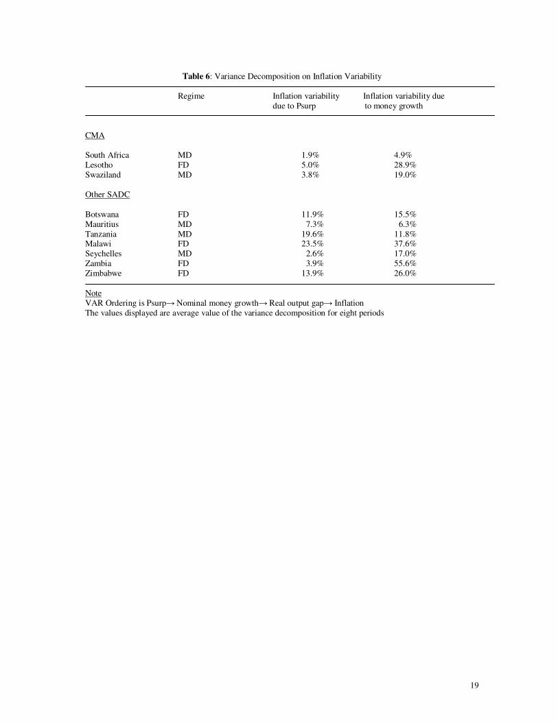
Table 6 summarizes the variance error decomposition results, suggesting that inflation
variability could be mostly explained by real primary surpluses (Mauritius and Tanzania),
money growth (Swaziland, Lesotho, Seychelles, Zambia and Zimbabwe) and by both
determinants (Malawi).
In table 6, second column, reports the regime identified by the previous approaches, while the
third and fourth columns show the average percentage of inflation variability for eight periods
due to, real primary surpluses and money growth respectively. Zimbabwe, for example, is a
case previously identified as a FD regime. Under this test, the inflation variability is more
likely to be associated with changes in money growth (26.0%) than changes in real surpluses

13
(13.9%), suggesting that the type of FD regime in Zimbabwe could be explained by the QTM
of debt monetisation. For Malawi, however, which is also a FD regime, the largest variability
in inflation is associated with both changes in real surpluses (23.5%) and money growth
(37.6%), indicating that the type of FD regime in Malawi could be best explained by both the
FTPD and QTM mechanisms. These results are also presented in figure 1.
Overall, these results seem to indicate that inflation variability could also be associated with
changes in real surpluses in countries under a MD regime, implying that real primary surpluses
matter to price volatility.
However, until now, we assume that there were no regime switches in our analysis. But
eyeballing rolling regression in government expenditure and revenue in figure 2, enables us see
if there is any significant changes taking place, particularly in the recent period. Notice the
difference between 1980-1994 and 1995-2005, for South Africa, Lesotho and Swaziland.
There is evidence of stabilisation policy in the later period than in the former. Movement in
government expenditure and revenue is more consistent and positive from 1995.
Similarly, for years, Botswana and Mauritius exhibit more positive and stable movement in
both variables. But, although insignificant, notice the recent negative change taking place in
Botswana, and a very strong and significant stability that is just occurring in Tanzania.
There is evidence of destabilisation policy in Malawi, Zambia and Zimbabwe.12 While that of
Seychelles shows a very high random movement in government expenditure and revenue. But
we did not attempt to formally identify statistical breaks in the data in order to confirm this,
which means that one may still need a more concrete evidence to support these changes.
V. CONCLUSION
This paper analyses the fiscal and monetary determinant of inflation in the SADC region. It
offers a theoretical model in understanding the implication of the FTPD in a small open
economy facing borrowing constraints. It provides quantitative evidence that traces out the
dynamic response of inflation to different shocks. In particular, the study finds, as predicted by
the FTPD, that changes in primary surplus pass through to prices by increasing inflation
variability. Therefore, fiscal policy matter for achieving and maintaining price stability in the
SADC region.
12
Again, although insignificant, notice the recent sign of a change towards stability in Malawi.
14
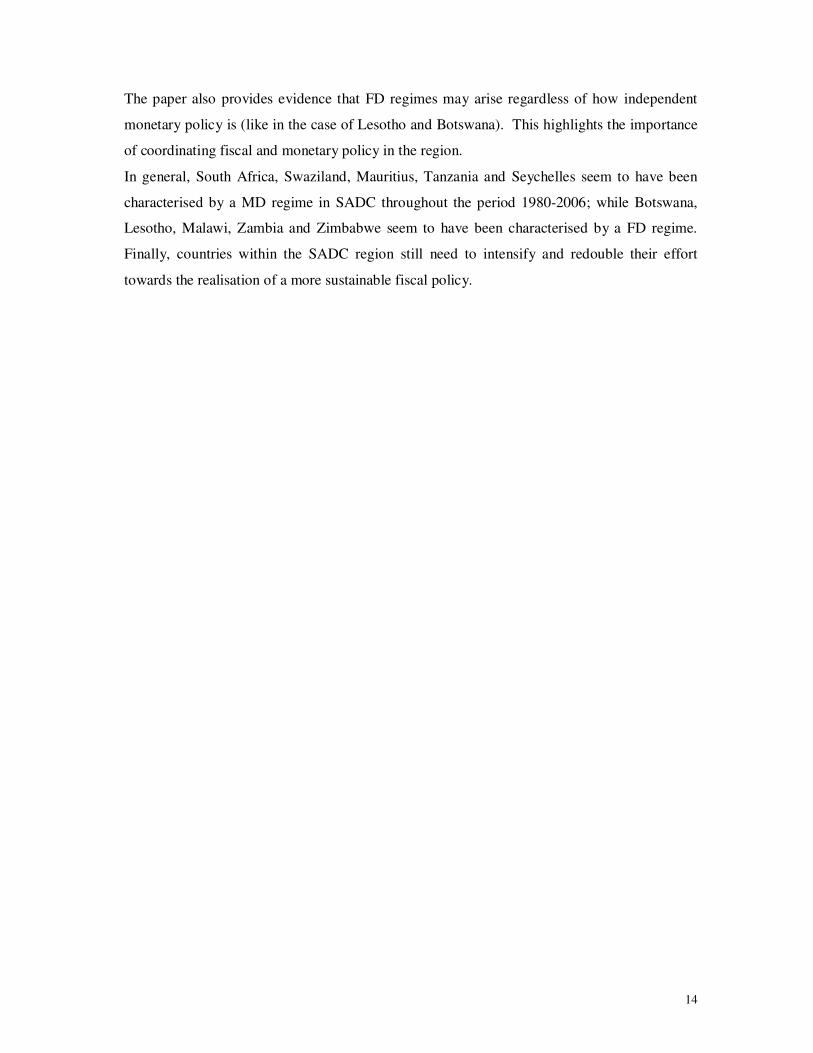
The paper also provides evidence that FD regimes may arise regardless of how independent
monetary policy is (like in the case of Lesotho and Botswana). This highlights the importance
of coordinating fiscal and monetary policy in the region.
In general, South Africa, Swaziland, Mauritius, Tanzania and Seychelles seem to have been
characterised by a MD regime in SADC throughout the period 1980-2006; while Botswana,
Lesotho, Malawi, Zambia and Zimbabwe seem to have been characterised by a FD regime.
Finally, countries within the SADC region still need to intensify and redouble their effort
towards the realisation of a more sustainable fiscal policy.

15
REFERENCES
Baldini, Alfredo and M.Ribeiro (2008) “Fiscal and Monetary Anchors for Price Stability:
Evidence from Sub-Saharan Africa”, IMF Working Paper /08/121
Buiter, Willem H. (2002), “The FISCAL Theory of the price Level: A Critique”, The
Economic Journal, 112 (July):459-480
. (1998), “The Young Person’s Guide to Neutrality, Price Level Indeterminacy, Interest
Rate Pegs, and the Fiscal Theories of the Price Level”, NBER Working Papers No..6396
Burnside, C, M. Eichenbaum and S. Rebello (2001), “Prospective Defects and the Asian
Currency Crisis, “Journal of Political Economy, 109 (6): 1155-1197
Canzoneri, Mathew; Cumby, Robert and Diba, Behzad (2001), Is the Price Level Determined by the Needs of Fiscal Solvency? American Economic Review, 9 (5), pp 1221-1238:
Christiano, Lawrence and Fitzgerald, Terry (2000), Understanding the Fiscal Theory of the
Price Level, National Bureau of Economic Research (Cambridge, MA) Working Paper No.
1050, April
Cochrane, John (1998), Long-term Debt and Optimal Policy in the Fiscal Theory of the price
Level, National Bureau of Economic Research (Cambridge, MA) Working Paper No.1050,
October
Enders, Walter (1995), Applied Econometric Time Series. New York: John Wiley & Sons, Inc
Enders, Walter (1996), RATS Handbook for Econometric Time Series. New York: John Wiley
& Sons, Inc
Favero, Carlo A. and Francesco Giavazzi (2004), Inflation Targeting and Debt: Lessons from Brazil, National Bureau of Economic Research (Cambridge, MA) Working Paper No. 1050,
march, pp1-4
Leeper, Eric M.(1991), Equlibria Under “Active” and “Passive” Monetary and Fiscal Policies, Journal of Monetary Economics, 27(1), pp 129-147
Loyo, E. (2000), in Sims, Christopher (2003)
McCallum, Bennett T (1999), Theoretical Issues Pertaining To Monetary Unions, NBER
Working Paper No 7393
Mankiw, Gregory N. (1999), Chapter 7: Macroeconomics. New York, Worth Publishers, pp
167-168
Marshall, Jeorge (2003), Fiscal Rule and Central Bank Issues in Chile, BIS Papers No.20, pp
98-99
Matallk, Ivan and Michal Slavik (2003), Fiscal Issues and Central Bank Policy in the Czech
Republic, BIS Papers, no.20, pp122-126

16
Mohanty, M.S. and Michela Scatigna (2003), Countercyclical Fiscal Policy and Central Bans,
BIS Papers, No. 20, pp38-39, 50-51
Moreno, Ramon (2003), Fiscal Issues and Central Banking in Emerging Economies: An
Overview, BIS Papers No.20, pp 6-7
Sala, Luca (2004) “The Fiscal Theory of the Price Level: Identifying Restrictions and Empirical Evidence,” IGIER Working Paper Series No 257
Sargent, Thomas J. and Neil Wallace (1981), Some Unpleasant Monetarist Arithmetic,
Quarterly Review Federal Reserve Bank, Fall, pp 1-2
Sidaoui, Jose (2003), Implications of Fiscal Issues for Central Banks: Mexico’s Experience, BIS Papers No.20, pp 180-181, 194
Sims, Christopher (1994), A Simple Model for Study of the Determination of the Price Level
and the Interaction of Monetary and Fiscal Policy, Economic Theory, 4(3), pp 381-399
. (1995), Economic Implications of the Government Budget Constraint, Moreno, Yale
University
Sokoler, Meir (2003), The Interaction Between Fiscal and Monetary Policy in Israel, BIS
Papers No.20, pp 158-159
Tanner, Evan and Alberto M. Ramos (2002) “Fiscal Sustainability and Monetary Versus Fiscal
Dominance: Evidence from Brazil, 1991-2000,” IMF Working Paper 02/5
Uribe, Jose Dario and Luis Ignacio Lazanio (2003), Fiscal Issues and Central Banks in
Emerging Markets: The Case of Columbia, BIS Papers No.20 pp 109-111
Woodford, Michael (1995), Price Level Determination without Control of a Monetary Aggregate, National Bureau of Economic Research (Cambridge, MA) Working Paper No.
1050, August, pp 1-27
(1996), “Control of the Public Debt: Requirement for Price Stability”, NBER Working
Papers, No. 5684
(1998), “Public Debt and the Price Level”, in Christiano et al (2000)

17
Table 1: Augmented Dickey-Fuller (ADF) Test for Unit Root
Country Stationary non Stationary
CMA
South Africa Psurp and Liab
Lesotho Psurp and Liab
Swaziland Psurp Liab
Other SADC
Botswana Psurp Liab
Mauritius Psurp Liab
Tanzania Psurp Liab
Malawi Psurp Liab
Seychelles Psurp and Liab
Zambia Psurp Liab
Zimbabwe Psurp Liab
Note
All monetary variables used in the analysis are stationary.
Table 2: Identification Criteria for Fiscal Dominance (FD) and Monetary Dominance (MD) Regimes
Criteria Response of future Liab to current Psurp Response of future Auto Psurp Regime
1st Order 2
nd Order Psurp to current Psurp
C1 negative (–) negative (–) positive (+) + MD
C2 non negative (0, +) non negative (0, +) non negative (0, +) + FD
C3 negative (–) negative (–) negative (–) – Unidentified
Note Psurb is government revenue less its expenditure (including net federal interest payment) and divided by nominal GDP. Liab is calculated by
adding the net federal debt to the money base both divided by nominal GDP. 1st VAR ordering is Psurp� Liab, which is consistent with a non Ricardian or FD regime characterized by an active fiscal policy.
2nd VAR ordering is Liab� Psurp, which is consistent with a Ricardian or MD regime characterized by a passive fiscal policy and active
monetary policy. Results are however, consistent under both orderings.
Table 3: Identification Criteria for FD and MD based on Nominal Income
Criteria Response of future income Response of future Psurp Regime
to current Psurp to current Psurp
C1 negative (–) positive (+) FD C2 positive (+) positive (+) MD
Note This is based on the sign of the impulse response function of the following VAR model; output gap� money growth� inflation

18
Table 4: VAR on Psurp and Liab
Response of future Liab to current Psurp Response of future Auto Psurp Regime
1st Order 2
nd Order Psurp to current Psurp
CMA
South Africa – + + + MD
Lesotho + + + + FD
Swaziland − – + + MD
Other SADC
Botswana + + + + FD
Mauritius − – + + MD
Tanzania − – + + MD
Malawi + + + + FD Seychelles – – + + MD
Zambia + + + + FD
Zimbabwe + + + + FD
Table 5: VAR on Log of Liab, Psurp and Log of Nominal GDP
Response of future nominal income to current Psurp Response of future Regime
1st Order 2
nd Order Psurp to current Psurp
CMA
South Africa 0/+ 0/+ + MD
Lesotho – – + FD
Swaziland 0/+ 0/+ + MD
Other SADC
Botswana – – + FD
Mauritius 0/+ 0/+ + MD
Tanzania 0/+ 0/+ + MD
Malawi – – + FD Seychelles 0/+ 0/+ + MD
Zambia 0/+ 0/+ + FD
Zimbabwe 0/+ 0/+ + FD
Note
VAR Ordering is log of nominal liabilities� Psurp� log of nominal income
19
Table 6: Variance Decomposition on Inflation Variability
Regime Inflation variability Inflation variability due
due to Psurp to money growth
CMA
South Africa MD 1.9% 4.9%
Lesotho FD 5.0% 28.9%
Swaziland MD 3.8% 19.0%
Other SADC
Botswana FD 11.9% 15.5%
Mauritius MD 7.3% 6.3%
Tanzania MD 19.6% 11.8% Malawi FD 23.5% 37.6%
Seychelles MD 2.6% 17.0%
Zambia FD 3.9% 55.6%
Zimbabwe FD 13.9% 26.0%
Note
VAR Ordering is Psurp� Nominal money growth� Real output gap� Inflation
The values displayed are average value of the variance decomposition for eight periods

20
Figure 1: Variance Decomposition on Inflation Variability
South Africa Lesotho Swaziland
0%
10%
20%
30%
40%
50%
60%
70%
80%
90%
100%
1 2 3 4 5 6 7 8
psurp mg ygap inf
0%
10%
20%
30%
40%
50%
60%
70%
80%
90%
100%
1 2 3 4 5 6 7 8
psurp mg ygap inf
0%
10%
20%
30%
40%
50%
60%
70%
80%
90%
100%
1 2 3 4 5 6 7 8
psurp mg ygap inf
Botswana Mauritius Tanzania
0%
10%
20%
30%
40%
50%
60%
70%
80%
90%
100%
1 2 3 4 5 6 7 8
psurp mg ygap Inf
0%
10%
20%
30%
40%
50%
60%
70%
80%
90%
100%
1 2 3 4 5 6 7 8
psurp mg ygap inf
0%
10%
20%
30%
40%
50%
60%
70%
80%
90%
100%
1 2 3 4 5 6 7 8
psurp mg ygap inf
Malawi Seychelles Zambia Zimbabwe
0%
10%
20%
30%
40%
50%
60%
70%
80%
90%
100%
1 2 3 4 5 6 7 8
psurp mg ygap inf
0%
10%
20%
30%
40%
50%
60%
70%
80%
90%
100%
1 2 3 4 5 6 7 8
psurp mg ygap inf
0%
1 0%
2 0%
3 0%
4 0%
5 0%
6 0%
7 0%
8 0%
9 0%
1 00%
1 2 3 4 5 6 7 8
psurp mg ygap inf
0%
10%
20%
30%
40%
50%
60%
70%
80%
90%
100%
1 2 3 4 5 6 7 8
psurp mg ygap inf

21
Figure 2: Rolling Regression in Government Expenditure and Revenue (% of GDP) 1980-2005
South Africa Lesotho Swaziland
-50
51
0m
os
es
_g
rev
1985 1990 1995 2000 2005Last obs. of sam ple
vs full-sample estimate
Coefficient on grev (95% CI)
Rolling regression estimates for gexp
-8
-6-4
-20
2m
os
es
_g
rev
1985 1990 1995 2000 2005Last obs. of sample
vs full-sample estimate
Coefficient on grev (95% CI)
Rolling regression estimates for gexp
-10
-50
51
0m
os
es
_g
rev
198 5 199 0 1 995 2 000 2 005Last obs. o f sample
vs ful l-sample estimate
Coeff icient on grev (95% CI)
Rolling regression estimates for gexp
Botswana Mauritius Tanzania
-10
12
mo
ses
_gre
v
1985 1990 1995 2000 2005Last obs. of sam ple
vs full-sample estimate
Coefficient on grev (95% CI)
Rolling regression estimates for gexp
-4-2
02
46
mo
ses
_gre
v
1985 1990 1995 2000 2005Last obs. of sam ple
vs full-sample estimate
Coefficient on grev (95% CI)
Rolling regression estimates for gexp
-10
-50
51
0m
ose
s_g
rev
1985 1990 1995 2000 2005Last obs. of sample
vs full-sample estimate
Coefficient on grev (95% CI)
Rolling regression estimates for gexp
Malawi Seychelles Zambia Zimbabwe
-15
-10
-50
51
0m
os
es_
gre
v
1985 1990 1995 2000 2005Last obs. of sample
vs ful l-sample estimate
Coefficient on grev (95% CI)
Rolling regression estimates for gexp
-20
24
6m
ose
s_
gre
v
1985 1990 1995 2000 2005Last obs. of sample
vs full-sam pl e est imate
Coefficient on grev (95% CI)
Rolling regression estimates for gexp
-10
-50
51
0m
os
es_
gre
v
1985 1990 1995 2000 2005Last obs . of sample
vs full-sample est imate
Coefficient on grev (95% CI)
Rolling regression estimates for gexp
-10
-50
51
0m
os
es_
gre
v
198 5 199 0 1 995 2 000 2 005Last obs. o f sample
vs ful l-sample estimate
Coeff icient on grev (95% CI)
Rolling regression estimates for gexp