how computers work - arsdigita...
TRANSCRIPT

How Computers Work Lecture 1 Page 1
How Computers Work
Subject Purpose
Introducing the Beta
Instruction Set Architecture

How Computers Work Lecture 1 Page 2
Subject Purpose
What’s Going on Behind That Screen?

How Computers Work Lecture 1 Page 3
Course Material• Web Site:
– Lecture Notes
– Reference Material• Today
– Beta Reference Material
• Instruction Set Reference
• Instruction Set Architecture
• Software Conventions
– Problem Sets
• Textbook– Hennesey and Patterson

How Computers Work Lecture 1 Page 4
Topics
(define (fact n)
(if (= n 0)
1
(* n (fact (- n 1)))
) )
(define (fact-iter n val)(if (= n 0)
val(fact-iter(- n 1)(* val n)
) ) )
Recursive approach Iterative approach (start val=1)

How Computers Work Lecture 1 Page 5
Review: From Scheme to SICP Register Machine Language
(define (fact-iter n val)(if (= n 0) val (fact-iter (- n 1) (* val n)))
) )
In SICP Register Machine Language
; Assumption: n = input, val = 1; Promise: val = n!
fact-iter:(test (op =) (reg n) (const 0))(branch (label done))(assign (reg val) (op *) (reg n) (reg val))(assign (reg n) (op -) (reg n) (const 1))(goto (label fact-iter))
done: (goto (reg continue))

How Computers Work Lecture 1 Page 6
So how do we execute SICP RML?
• What do we need?– Memory
• To store program instructions• To store intermediate data values
– Calculator• To carry out calculations• Commonly called an “ALU”, which stands for Arithmetic / Logic Unit
– Instruction Set Architecture• Describes format of program instructions
– One example: SICP RML (not very practical)
– Another example: the “Beta” (more representative of real machines)
– Control Machine• To interpret the instructions and tell the data memory and ALU what
to do.

How Computers Work Lecture 1 Page 7
What else do we need?
• A PC or Program Counter to keep track of where we are in the program memory.
• A way of controlling the PC depending on if statements (conditionals).
• Some method of remembering where we’ve been when doing recursive calls, because the PC isn’t enough
• Some method of managing memory for subroutine calls, heap storage, etc ...

How Computers Work Lecture 1 Page 8
What should the program instructions look like?
• They need to specify what calculation (operation) should be done on the data
• They need to specify what data should be used for the calculation.
• They need to specify where in the data memory the result should be stored.
• Attempt #1:
OPCODE SRC_PTR_1 SRC_PTR_2 DEST_PTR
E.G. ADD 43264 932643 43265
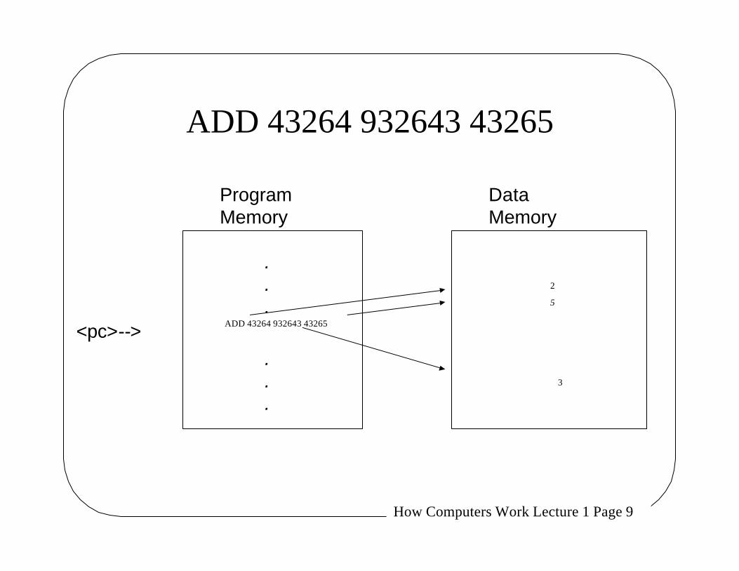
How Computers Work Lecture 1 Page 9
ADD 43264 932643 43265
ADD 43264 932643 43265
.
.
.
.
.
.
<pc>-->
2
3
ProgramMemory
DataMemory
5

How Computers Work Lecture 1 Page 10
What’s Wrong with this?
• If we have lots of data, the pointers into data memory can become very Wide
• If the pointers are very Wide, then the instructions will need to be very Wide.
• Other problems: The nature of memory systems.

How Computers Work Lecture 1 Page 11
The Ideal Memory System
FastCheap (Large)
SALE
How Computers Work Lecture 1 Page 12
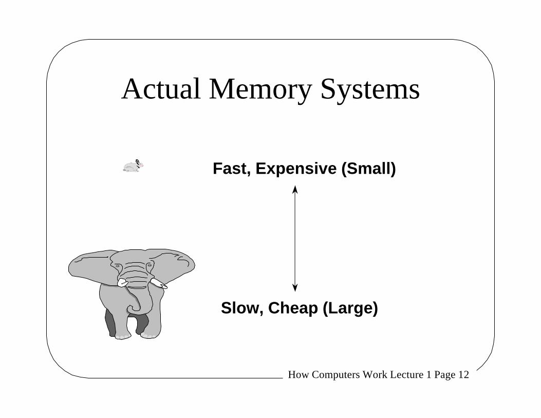
Actual Memory Systems
Fast, Expensive (Small)
Slow, Cheap (Large)

How Computers Work Lecture 1 Page 13
Why Big Data Memories are Slow
• The more selection a chip needs to do, the longer it takes to find the data being selected.
• Big memories are off-chip, and communications within an integrated circuit are fast, communications between chips are slow.

How Computers Work Lecture 1 Page 14
Can we do this?
+
=
A: Consider your bookshelf and the library

How Computers Work Lecture 1 Page 15
Locality

How Computers Work Lecture 1 Page 16
A good idea:• Invent a small “register file” which most instructions will point to for
data source and destination.
• Invent new Memory-type instructions for– Loading data from the bigger data memory to the register file
– Storing data to the bigger data memory from the register file
• New ALU-type instruction format
e.g. ADD R0 R1 R2
e.g. LD 43264, R0LD 932643, R1
ST R2, 43265

How Computers Work Lecture 1 Page 17
Instruction Set Design
• Wide choice in # of addresses specified– 0 address (stack) machines (e.g. Java virtual machine)
– 1 address (accumulator) (e.g. 68hc11)
– 2 address machines (e.g. Dec PDP-11)
– 3 address machines (e.g. Beta)
• Wide choice of complexity of instructions– CISC vs. RISC (e.g. I86 vs. Beta)

How Computers Work Lecture 1 Page 18
β Model of Computation
PC
r0r1r2
r31
32 bits
always 0
Processor State
32 bits(4 bytes)
Instruction Memory
next instr
• Fetch <PC>
• PC ←← <pc> + 1
• Execute fetched instruction
• Repeat!
Fetch/ExecuteLoop:
How Computers Work Lecture 1 Page 19
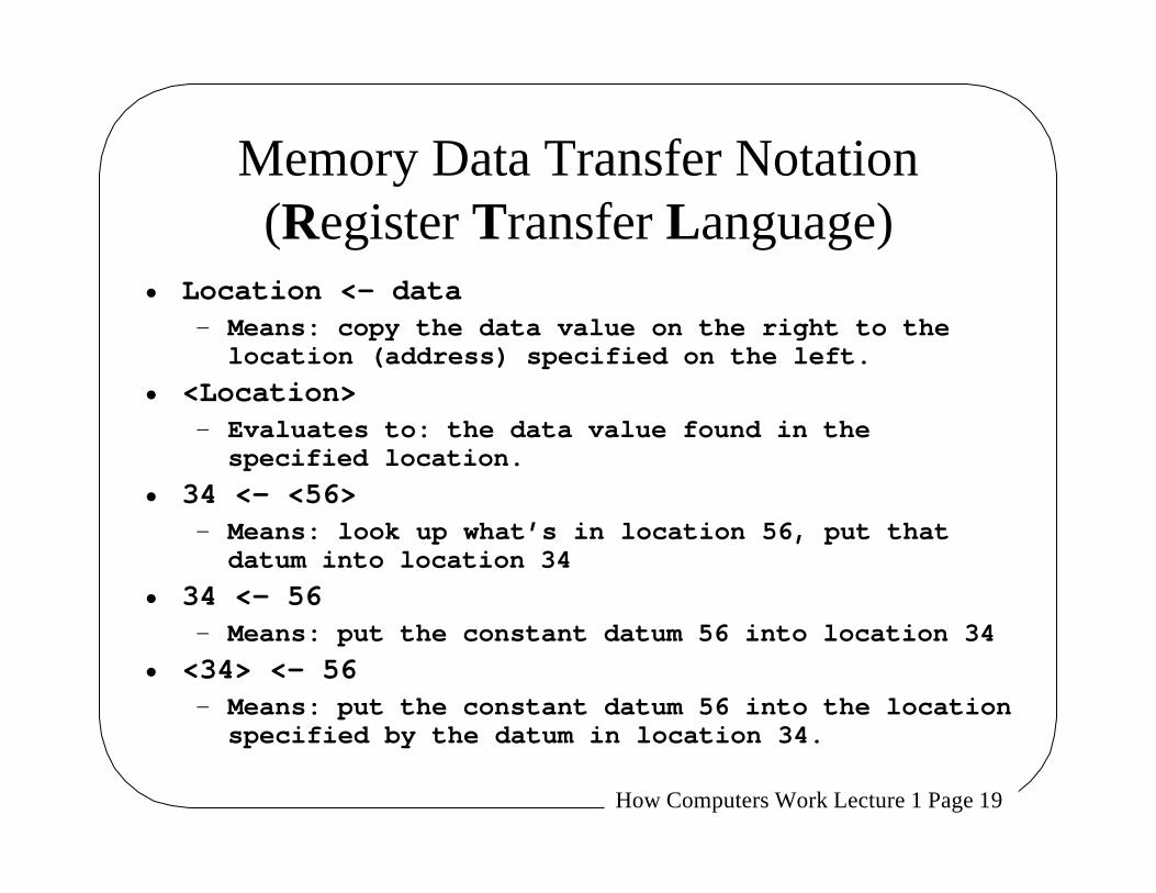
Memory Data Transfer Notation(Register Transfer Language)
• Location <- data– Means: copy the data value on the right to the
location (address) specified on the left.
• <Location> – Evaluates to: the data value found in the
specified location.
• 34 <- <56>– Means: look up what’s in location 56, put that
datum into location 34
• 34 <- 56– Means: put the constant datum 56 into location 34
• <34> <- 56– Means: put the constant datum 56 into the location
specified by the datum in location 34.

How Computers Work Lecture 1 Page 20
BETA Instructions
Two 32-bit Instruction Formats:
Unused RcRaOPCODE Rb
OPCODE Ra 16 bit Constant Rc

How Computers Work Lecture 1 Page 21
β ALU Operations
ADD(ra, rb, rc) rc ←← <ra> + <rb>
What the machine sees (32-bit instruction word):
What we prefer to see: symbolic ASSEMBLY LANGUAGE
Alternative instruction format:
ADDC(ra, const, rc) rc ←← <ra> + sext(const)
“Add the contents of ra to the contents ofrb; store the result in rc”
SIMILARLY FOR:
• SUB, SUBC• (optional)
MUL, MULCDIV, DIVC
BITWISE LOGIC:• AND, ANDC• OR, ORC• XOR, XORC
SHIFTS:• SHL, SHR, SAR
(shift left, right;shift arith right)
“Add the contents of ra to const; store the result in rc”
Unused RcRaOPCODE Rb
OPCODE Ra 16 bit Constant Rc
How Computers Work Lecture 1 Page 22
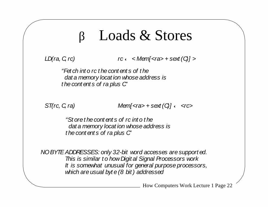
β Loads & Stores
LD(ra, C, rc) rc ←← < Mem[<ra> + sext(C)] >
ST(rc, C, ra) Mem[<ra> + sext(C)] ←← <rc>
“Fetch into rc the contents of thedata memory location whose address is
the contents of ra plus C”
“Store the contents of rc into thedata memory location whose address is
the contents of ra plus C”
NO BYTE ADDRESSES: only 32-bit word accesses are supported.This is similar to how Digital Signal Processors workIt is somewhat unusual for general purpose processors,which are usual byte (8 bit) addressed

How Computers Work Lecture 1 Page 23
β Branches
Note: “displacement” is coded as a
CONSTANT in a field of the instruction!
Conditional: rc = <PC>+1; then
BRNZ(ra, label, rc) if <ra> nonzero then
PC <- <PC> + displacement
BRZ(ra, label, rc) if <ra> zero then
PC <- <PC> + displacement
Unconditional: rc = <PC>+1; then
BRZ(r31, label, rc) PC <- <PC> + displacement
Indirect: rc = <PC>+1; then
JMP(ra, rc) PC <- <ra>

How Computers Work Lecture 1 Page 24
Run-time Discipline: Ground rules•Instruction live in Big Memory
•ALU Operates on Registers
•Variables live in Big Memory
•Ergo: Registers hold Temporary values
1000:1001:1002:
1004:1003:
xy
(let ((x 0)(y 0)
)(set! y (* x 37))
)
LD(r31, 0x1002, r0)MULC(r0, 37, r0)ST(r0, 0x1003, r31)
x=0x1002 ; variable xy=0x1003 ; variable yLD(x, r0) ; r0 gets xMULC(r0, 37, r0) ; r0 gets x*37ST(r0, y) ; y gets x*37
translatesto
or, morehumanely,
to

How Computers Work Lecture 1 Page 25
Translation of an Expression
c:
x:y:
123456
• VARIABLES translate to LD or ST
• OPERATORS translate to ALU instructions
• SMALL CONSTANTS translate to “literal-mode” ALU instructions
• LARGE CONSTANTS translate to LD Instruction (or LDR)
(let ((x 0)(y 0)(c 123456)
)(set! y (* (+ c y) (- x 3)))
)
x: 0
y: 0
c: 123456
...
LD(x, r1)
SUBC(r1,3,r1)
LD(y, r2)
LD(c, r3)
ADD(r2,r3,r2)
MUL(r2,r1,r1)
ST(r1,y)

How Computers Work Lecture 1 Page 26
Our Favorite Program
; assume n is 20, val is 1
(define (fact-iter n val)(if (= n 0)
val(fact-iter(- n 1)(* val n))
) ) )
n: 20val: 1
loop:LD(n, r1)CMPEQ(r31, r1, r2)BRNZ(r2, done)
LD(val, r3)MUL(r1, r3, r3)ST(r3,val)SUBC(r1, 1, r1)ST(r1, n)BR(loop)
done:

How Computers Work Lecture 1 Page 27
Optimizing ...; assume n is 20, val is 1
(define (fact-iter n val)(if (= n 0)
val(fact-iter(- n 1)(* val n))
) ) )
n: 20val: 1
LD(n, r1) ; n in r1LD(val, r3) ; accum in r3
loop:CMPEQ(r31, r1, r2)BRNZ(r2, done)MUL(r1, r3, r3)SUBC(r1, 1, r1)BR(loop)
done:ST(r1, n) ; new nST(r3, val) ; new accum
Cleverness:We move LDs/STs out of loop!
(Still, 5 instructions in loop...)

How Computers Work Lecture 1 Page 28
REAL Hacking: 3-instruction Loop; assume n is 20, val is 1
(define (fact-iter n val)(if (= n 0)
val(fact-iter(- n 1)(* val n))
) ) )
Cleverness:We avoid conditional overhead
(Now 3 instructions in loop!)
n: 20val: 1
LD(n, r1) ; n in r1LD(val, r3) ; val in r3BRZ(r1, done)
loop:MUL(r1, r3, r3)SUBC(r1, 1, r1)BRNZ(r1, loop)
done:ST(r1, n) ; new nST(r3, val) ; new accum

How Computers Work Lecture 1 Page 29
Language ToolsThe Beta Assembler
Assembler01101101110001100010111110110001.....
SymbolicSOURCEtext file
BinaryMachine
Language
Translatorprogram
STREAM of Wordsto be loadedinto memory
TextualMacroPre-Processor
SymbolMemory +ExpressionEvaluator
How Computers Work Lecture 1 Page 30
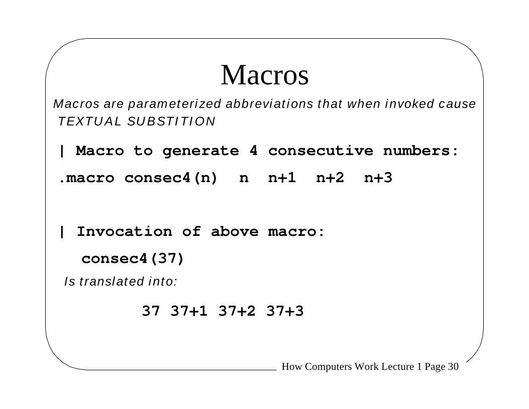
Macros
| Macro to generate 4 consecutive numbers:
.macro consec4(n) n n+1 n+2 n+3
| Invocation of above macro:
consec4(37)
37 37+1 37+2 37+3
Is translated into:
Macros are parameterized abbreviations that when invoked causeT E X T U A L S U B S T I T I O N

How Computers Work Lecture 1 Page 31
Some Handy Macros
| BETA Instructions:
ADD(ra, rb, rc) | rc ←← <ra> + <rb>ADDC(ra, const, rc) | rc ←← <ra> + constLD(ra, C, rc) | rc ←← <C + <ra>>ST(rc, C, ra) | C + <ra> ←← <rc>LD(C, rc) | rc ←← <C>ST(rc, C) | C ←← <ra>

How Computers Work Lecture 1 Page 32
Constant Expression Evaluation37 -3 255
0x25
0b100101
decimal (default);
binary (0b prefix);
hexadecimal (0x prefix);
Values can also be expressions; eg:
37+0b10-0x10 24-0x1 4*0b110-1 0xF7&0x1F
generates 4 words of binary output, each with the value 23
How Computers Work Lecture 1 Page 33
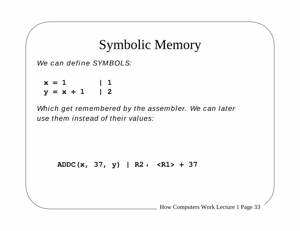
Symbolic MemoryWe can def ine SYMBOLS:
x = 1 | 1y = x + 1 | 2
ADDC(x, 37, y) | R2 ←← <R1> + 37
Which get remembered by the assembler. We can later use them instead of their values:

How Computers Work Lecture 1 Page 34
How Are Symbols Different Than Macros?
• Answer:– A macro’s value at any point in a file is the last
previous value it was assigned.• Macro evaluation is purely textual substitution.
– A symbol’s value throughout a file is the very last value it is assigned in the file.
• Repercussion: we can make “forward” references to symbols not yet defined.
• Implementation: the assembler must first look at the entire input file to define all symbols, then make another pass substituting in the symbol values into expressions.

How Computers Work Lecture 1 Page 35
Dot, Addresses, and Branches
Special symbol “.” (period) changes to indicate the address of the next output byte.
.macro BRNZ(ra,loc) betaopc(0x1E,ra,(loc-.)-1,r31)
loop = . | “loop” is here...ADDC(r0, 1, r0)...BRNZ(r3, loop) | Back to addc instr.
We can use . to define branches to compute RELATIVE address field:

How Computers Work Lecture 1 Page 36
Address Tags
x: 0
buzz: LD(x, r0) do { x = x-1; }ADDC(r0, -1, r0)ST(r0, x)BRNZ(r0, buzz) while (x > 0);...
x: is an abbreviation for x =. - - leading to programs like

How Computers Work Lecture 1 Page 37
Macros Are Also Distinguished by Their Number of Arguments
We can extend our assembly language with new macros. For example,we can def ine an UNCONDITIONAL BRANCH:
BR(label, rc) rc ←← <PC>+4; then
PC ←← <PC> + displacement___________________________________________
BR(label) PC ←← <PC> + displacement
.macro BR(lab, rc) BRZ (r31,lab, rc)
by the definitions
.macro BR(lab) BR(lab,r31)

How Computers Work Lecture 1 Page 38
What Did We Do Today?• The beta instruction set architecture
• How to do iterative factorial in the beta ISA
• The 6.004 macro-assembler
What will we do next lecture?
What will you do in section?• Review of how the Macro Assembler works
• Practice with the Beta ISA
• Representation of data in binary
– Bools, Chars, (many reperesentations of Ints)• Big and Little Endians
• Everything you always wanted to know about sext(C)
• Function Calling
• Recursive Factorial