how can marine biologists track sperm whales in...

Chapter 6

How can marine biologists track sperm whales in

the oceans?

Hear they are!

T. Dutoit (°), V. Kandia(+), Y. Stylianou (*)

(°) Faculté Polytechnique de Mons, Belgium

(+) Foundation for Research and Technology-Hellas, Heraklion, Greece

(*) University of Crete, Heraklion, Greece

Whale watching has become a trendy occupation these last years. It is

carried on in the waters of some 40 countries, plus Antarctica. Far beyond

its touristic aspects, being able to spot the position of whales in real time

has several important scientific applications, such as censusing (estimation

of animal population), behavior studies and mitigation efforts concerning

fatal collisions between marine mammals and ships and exposure of ma-

rine mammals to loud sounds of anthropogenic origin (seismic surveys, oil

and gas exploitation and drilling, naval and other uses of sonar).

When whales do not appear on the surface of water, one way of detect-

ing their position is to listen to the sounds they emit through several fixed

hydrophones (i.e., microphones specially designed for underwater use).

Hydrophone signals are then processed with a SOund Navigation And

Ranging (sonar) technique, which uses sound propagation under water to

detect and spot objects. In this Chapter, we thus plunge deep into underwa-

ter acoustics, by examining a proof of concept for sperm whale tracking

http://en.wikipedia.org/wiki/Sound

186 T. Dutoit, V. Kandia, Y. Stylianou

using passive acoustics1, and based on the estimation of the cross-

correlation between hydrophone signals to spot whales on a 2D map.

6.1 Background – Source localization

We start by examining sperm whale sounds (Section 6.1.1), and show how

the Teager-Kaiser operator efficiently increases the signal-to-noise ratio of

hydrophone signals (Section 6.1.2).

Sperm whale sounds are actually received by hydrophones at slightly

different times, due to the various distances between the animal and the

hydrophones. Knowing the location of the hydrophones, the time differ-

ence of arrival (TDOA) between pairs of hydrophones can be obtained, us-

ing various techniques (Sections 6.1.3 and 6.1.4), and provided to a multi-

lateration algorithm (Section 6.1.5) for determining the position of the

animal.

6.1.1 Sperm whale sounds

Sperm whales are highly vocal active animals. An adult sperm whale pro-

duces some 25000 clicks a day. If we consider that the heart rate of such a

large whale is around 15 beats per minute (i.e., 20000 beats a day), sperm

whale produces more clicks than heart beats (Madsen 2002). Their reper-

toire is made up almost entirely of a number of click types with different

properties.

Usual (or regular) clicks (Fig. 6.1) are the most commonly heard click

type during deep foraging dives, and are therefore used to locate the ani-

mals using passive acoustic methods. They are impulsive broadband

sounds of multi-pulse structure with inter-click interval (ICI) between

0.5s-1s. Usual clicks are highly directional sounds with source levels up to

235 dB rms re 1µPa2. It is believed that these properties represent adapta-

tions for long-range echolocation.

1 Sonars can be active or passive. Passive sonars only listen to their surrounding,

while active sonars emit sounds and detect echoes from their surrounding.

Whales and dolphins use echolocation systems similar to active sonars to locate

predators and preys; marine biologists listen to the resulting sounds and echoes

(hence, in a passive set-up) to detect cetaceans. 2 For underwater sound, 1 μPa is the reference pressure level. Since the measured

pressure level from a particular sound source decreases with distance from the

source, the convention is to use one meter as a reference distance. Thus, the

How can marine biologists track sperm whales in the oceans? 187

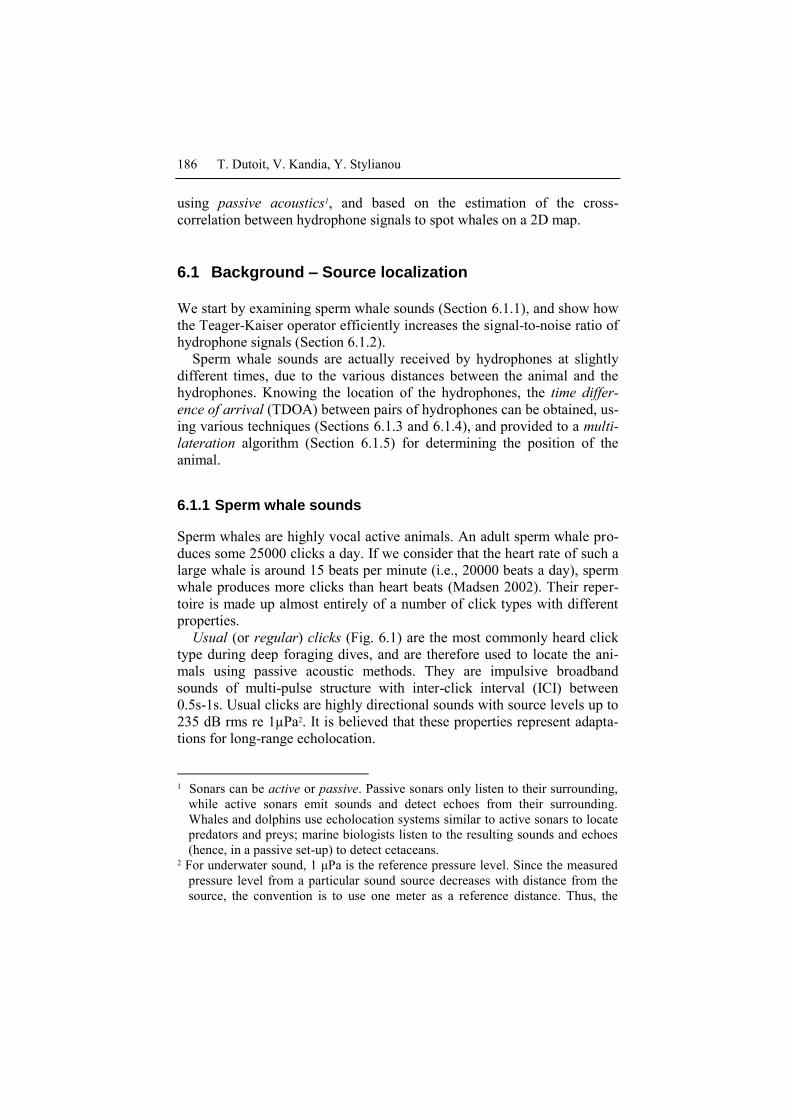
Fig. 6.1 Left: Sequence of usual sperm whale clicks. Each click is followed by an

echo, due to surface reflection3. Right: zoom on a single click, showing the multi-

pulse structure of the signal. The notation on pulses follows that of (Møhl et al.

2000, Zimmer et al. 2005)

Creak clicks (Fig. 6.2) are burst of mono-pulsed clicks with high repeti-

tion rate (up to 200 clicks per second). They are highly directional sounds

with source level between 180-205 dB rms re 1µPa. They are produced

during foraging dives and it is believed that they have a function analogous

to the terminal buzzes produced by bats during echolocation 4.

Several other types of sounds are also encountered, such as coda clicks,

chirrup clicks, slow clicks, squeals, and trumpets, most of which have a

social communicative role. 5

pressure level from a sound source is measured in “dB rms re 1μPa at 1m” (and

the "at 1m" is usually omitted). 3 Hydrophones are mounted at roughly 5m off the bottom, so that reflection from

the bottom comes with a ~7ms delay, i.e. inside the direct path click itself. Fur-

thermore, the hydrophones have an upward directed beam pattern. 4 After detecting a potential prey using low rate echolocation calls, bats emit a

characteristic series of calls at a high repetition rate (a terminal buzz) to localize

the prey. 5 For more information on sperm whale sounds, please refer to Madsen 2002,

Drouot 2003, Teloni et al. 2005.


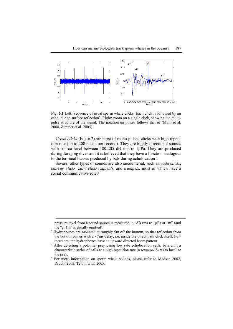
Fig. 6.2 Left: Segment of a creak, composed of several clicks (and their echoes)

in high amplitude noise. Right: zoom on a single click of the segment, which

shows the mono-pulse nature of the sound.

As shown in Fig. 6.1 and Fig. 6.2, hydrophone signals exhibit very low

signal-to-noise ratios. In particular they are often contaminated by low-

frequency noise, mostly due to human activity. Shipping indeed, which ac-

counts for more of 75% of all human sound in the sea (ICES 2005), pro-

duces low-frequency sounds (rumble of engines, propellers). Commercial

shipping traffic is growing as does the tonnage (cargo capacity) of ships,

adding more noise in the low frequency band.

6.1.2 The Teager-Kaiser energy operator

The Teager–Kaiser (TK) energy operator is defined in the continuous do-

main as:

[ ( )] ( )² ( ) ( )TK x t x t x t x t (6.1)

where x and x denote the first and second derivative over time, respec-

tively. For a discrete time signal, it is shown in (Kaiser 1990) that the TK

energy operator is given by:

[ ( )] ²( ) ( 1) ( 1)TK x n x n x n x n (6.2)

The TK operator is referred to as energy operator because it is related to

the concept of energy in the generation of acoustic waves (Kaiser 1990).

This operator can be seen as a special case of quadratic filters defined

by:


1 2

1 2 1 2( ) ( , ) ( ) ( )i i

y n h i i x n i x n i

(6.3)

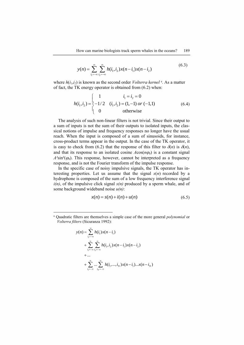
where h(i1,i2) is known as the second order Volterra kernel 6. As a matter

of fact, the TK energy operator is obtained from (6.2) when:

1 2

1 2 1 2

1 0

( , ) 1/ 2 ( , ) (1, 1) ( 1,1)

0 otherwise

i i

h i i i i or

(6.4)

The analysis of such non-linear filters is not trivial. Since their output to

a sum of inputs is not the sum of their outputs to isolated inputs, the clas-

sical notions of impulse and frequency responses no longer have the usual

reach. When the input is composed of a sum of sinusoids, for instance,

cross-product terms appear in the output. In the case of the TK operator, it

is easy to check from (6.2) that the response of this filter to (n) is (n),

and that its response to an isolated cosine Acos(n0) is a constant signal

A²sin²(0). This response, however, cannot be interpreted as a frequency

response, and is not the Fourier transform of the impulse response.

In the specific case of noisy impulsive signals, the TK operator has in-

teresting properties. Let us assume that the signal x(n) recorded by a

hydrophone is composed of the sum of a low frequency interference signal

i(n), of the impulsive click signal s(n) produced by a sperm whale, and of

some background wideband noise u(n):

( ) ( ) ( ) ( )x n s n i n u n (6.5)

6 Quadratic filters are themselves a simple case of the more general polynomial or

Volterra filters (Sicuranza 1992):

1

1 2

1

1 1

1 2 1 2

1 1

( ) ( ) ( )

( , ) ( ) ( )

...

... ( ,..., ) ( )... ( )N

i

i i

N N

i i

y n h i x n i

h i i x n i x n i

h i i x n i x n i


If the interference frequency is low and the signal-to-noise ratio (SNR) be-

tween the impulsive clicks and the background noise is sufficient, it is

shown in (Kandia and Stylianou 2005) that the TK operator has the very

interesting property of ignoring the interference component while increas-

ing the SNR (Fig. 6.3). Moreover, it does not smear input pulses in time

(Fang and Atlas 1995). As a matter of fact, if we neglect the influence of

the noise u(n) and identify x(n) to a Dirac pulse (n) and i(n) in the vicinity

of this pulse to a constant value K, it is easy to show from (6.2) that the

output y(n) of the TK filter only has three non zero samples:

1

( ) 1 2 0

1

K n

y n K n

K n

(6.6)

TK

TK

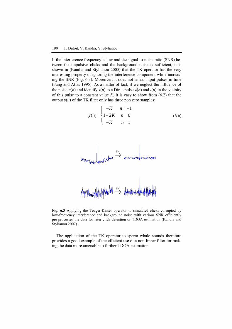
Fig. 6.3 Applying the Teager-Kaiser operator to simulated clicks corrupted by

low-frequency interference and background noise with various SNR efficiently

pre-processes the data for later click detection or TDOA estimation (Kandia and

Stylianou 2007).

The application of the TK operator to sperm whale sounds therefore

provides a good example of the efficient use of a non-linear filter for mak-

ing the data more amenable to further TDOA estimation.


6.1.3 TDOA estimation based on the generalized cross correlation

Let us assume that signals x1(t) and x2(t) result from the propagation of

signal s(t) through different paths that are identified to a simple attenuation

and a delay:

( ) ( ) ( )i i i ix t a s t b t (6.7)

where bi(t) (i=1,2) are zero-mean, uncorrelated stationary random proc-

esses, which are also non-correlated with s(t).

The cross power spectrum density (PSD) 1 2

( )x xS f between x1 and x2 is

given by:

1 2 1 2

12

12

2

2 2

1 2

2

1 2

( ) ( )

( )

( )

j ft

x x x x

j f j ft

ss

j f

ss

S f t e dt

a a e t e dt

a a e S f

(6.8)

in which 1 2

( )x x t is the cross correlation between x1(t) and x2(t) , ( )ss t is

the autocorrelation of s(t), and ( )ssS f is therefore the PSD of s(t).

Knapp and Carter (1976) have proposed to estimate the time difference

of arrival TDOA 12 = 1-2 between x1(t) and x2(t), as the position of the

maximum of the generalized cross correlation function, defined as:

1 2 1 2

2( ) ( ) ( ) j f

x x x xf S f e df

(6.9)

in which (f) is a weighting function.

In particular, when (f) is set to 1, 1 2

( )x x is the inverse Fourier Trans-

form of the cross PSD, i.e., the standard cross-correlation function. For

signals verifying (6.8), this leads to have:

1 2 1 2 12( ) ( )x x ssa a (6.10)

in which ( )ss is the autocorrelation function of s(t). Since the maximum

of ( )ss is always found at = 0, 12 can be estimated as the position of


the maximum of (6.10). However, if b1(t) and b2(t) exhibit some cross-

correlation, (6.10) becomes:

1 2 1 21 2 12( ) ( ) ( )x x ss b ba a (6.11)

whose maximum may not correspond to 12. In particular, if bi(t) are sinu-

soidal components with the same frequency, a sinusoidal term will appear

in (6.11), due to a spectral line in 1 2

( )x xS f .

When (f) is set to 1/|1 2

( )x xS f |, we obtain the so-called phase trans-

form, which computes the generalized cross correlation from the phase of

the cross PSD. For signals verifying (6.8), the phase transform still pro-

vides a perfect estimate of 12, since:

1 2 12

1 2

1 2

2( )

( ) ( )| ( ) |

x x j f

x x

x x

S ff S f e

S f

(6.12)

which leads to:

1 2 12( ) ( )x x (6.13)

Now if bi(t) are sinusoidal components with the same frequency, their con-

tributions to 1 2

( )x x will be much lower than in (6.11), since the spectral

line in 1 2

( )x xS f will be canceled in (6.12). This makes the phase transform

an interesting estimator, provided 1 2

( )x xS f can itself be correctly esti-

mated.

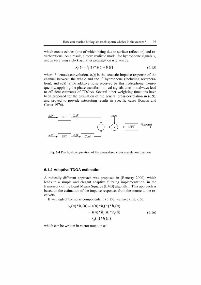
In practice, 1 2

( )x xS f is estimated in [0, Fs] from a finite number of

samples of x1(n) and x2(n), as (Fig. 6.4):

1 2

*

1 2( ) ( ) ( ) ( 0,..., 1)sx x

FS k X k X k k N

N (6.14)

where Xi(k) (i=1,2) is the N-point Discrete Fourier Transform of the se-

quence [ ( ), ( 1), , ( 1)i i ix n x n x n N ]. This is known to give a biased

but consistent estimation of 1 2

( )x xS f .

TDOA estimation from real signals is not so easy. As mentioned above,

hydrophone signals are polluted with interference signals and additive

noise due to surrounding sources other than the one we want to spot. More

annoyingly, several propagation paths may exist to each hydrophone: typi-

cally a direct path with lowest attenuation plus many secondary paths,


which create echoes (one of which being due to surface reflection) and re-

verberations. As a result, a more realistic model for hydrophone signals x1

and x2 receiving a click s(t) after propagation is given by:

( ) ( )* ( ) ( )i i ix t h t s t b t (6.15)

where * denotes convolution, hi(t) is the acoustic impulse response of the

channel between the whale and the ith hydrophone (including reverbera-

tion), and bi(t) is the additive noise received by this hydrophone. Conse-

quently, applying the phase transform to real signals does not always lead

to efficient estimates of TDOAs. Several other weighting functions have

been proposed for the estimation of the general cross-correlation in (6.9),

and proved to provide interesting results in specific cases (Knapp and

Carter 1976).

FFT

FFT

x

Conj

X1(k)

X2(k)

IFFT x

(k)

x1x2(n)

k)

x1(n)

x2(n)

Fig. 6.4 Practical computation of the generalized cross correlation function

6.1.4 Adaptive TDOA estimation

A radically different approach was proposed in (Benesty 2000), which

leads to a simple and elegant adaptive filtering implementation, in the

framework of the Least Means Squares (LMS) algorithm. This approach is

based on the estimation of the impulse responses from the source to the re-

ceivers.

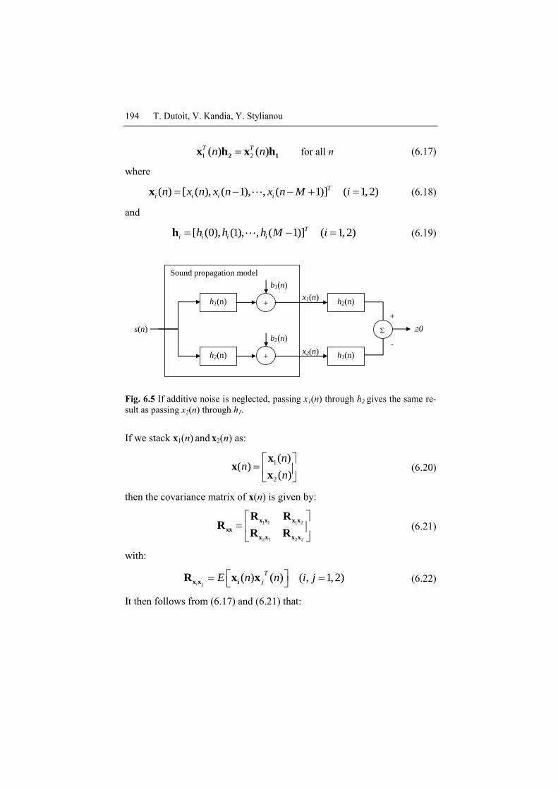
If we neglect the noise components in (6.15), we have (Fig. 6.5):

1 2 1 2

2 1

2 1

( )* ( ) ( )* ( ) * ( )

( )* ( )* ( )

( )* ( )

x n h n s n h n h n

s n h n h n

x n h n

(6.16)

which can be written in vector notation as:


1 2( ) ( )T Tn n2 1x h x h for all n (6.17)

where

( ) [ ( ), ( 1), , ( 1)] ( 1,2)T

i i i in x n x n x n M i x (6.18)

and

[ (0), (1), , ( 1)] ( 1,2)T

i i i ih h h M i h (6.19)

Sound propagation model

s(n)

h1(n)

h2(n)

+

+

b1(n)

b2(n)

+

-

0

h2(n)

h1(n)

x1(n)

x2(n)

Fig. 6.5 If additive noise is neglected, passing x1(n) through h2 gives the same re-

sult as passing x2(n) through h1.

If we stack x1(n) and x2(n) as:

1

2

( )( )

( )

nn

n

xx

x (6.20)

then the covariance matrix of x(n) is given by:

1 1 1 2

2 1 2 2

x x x x

xx

x x x x

R RR

R R (6.21)

with:

( ) ( ) ( , 1,2)i j

T

jE n n i j x x iR x x (6.22)

It then follows from (6.17) and (6.21) that:


0 with

2

1

hRu u

h (6.23)

This remarkably simple result provides a simple means of estimating the

impulse responses h1 and h2 from the estimation of xxR .

In practice, though, accurate estimation of u is not trivial, as the impulse

responses may be long, and background noise may falsify (6.23). Benesty

(2000) has therefore proposed an adaptive estimation of u, based on a

Least Means Squares (LMS) principle. The idea is to find an error function

e(n) such that the expectation E[e²(n)] is minimized when (6.23) is veri-

fied, and such that the gradient of E[e²(n)] with respect to u has a simple

analytical form. Clearly, e(n)=uTx meets these requirements, as

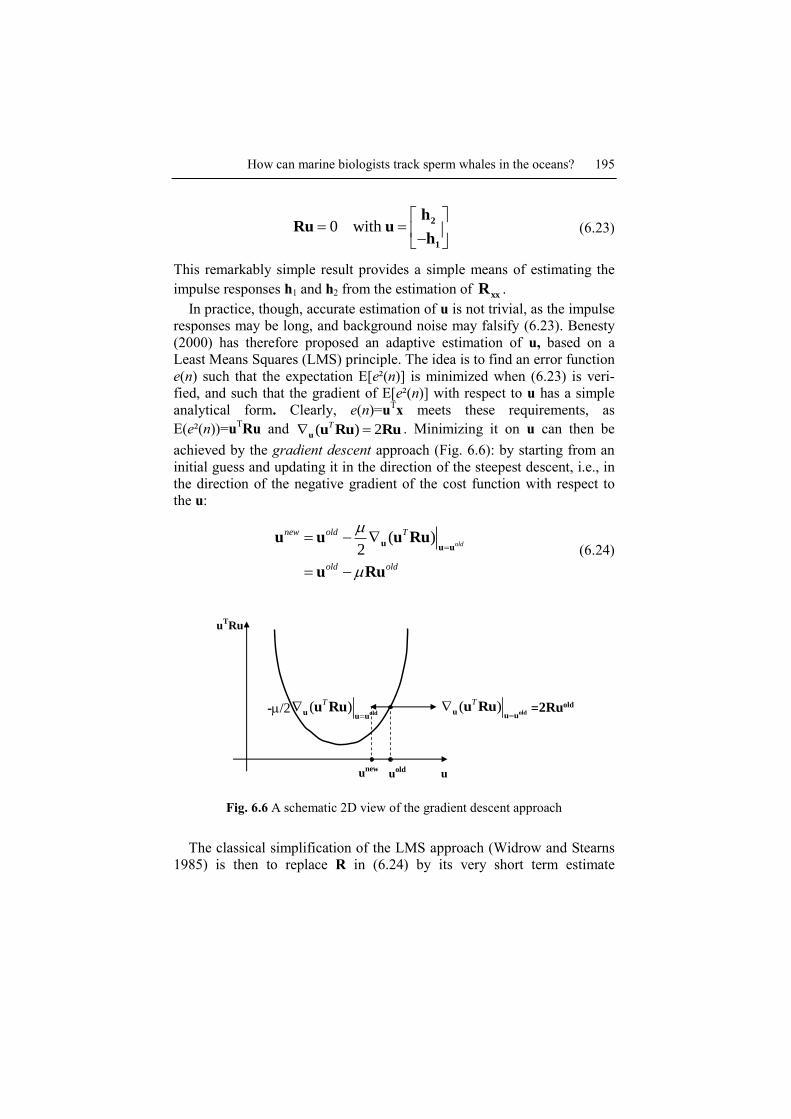
E(e²(n))=uTRu and ( ) 2T u u Ru Ru . Minimizing it on u can then be

achieved by the gradient descent approach (Fig. 6.6): by starting from an

initial guess and updating it in the direction of the steepest descent, i.e., in

the direction of the negative gradient of the cost function with respect to

the u:

( )2

old

new old T

old old

uu u

u u u Ru

u Ru

(6.24)

uTRu

u

( )T

olduu u

u Ru =2Ruold -/2 ( )T

olduu u

u Ru

uold

unew

Fig. 6.6 A schematic 2D view of the gradient descent approach

The classical simplification of the LMS approach (Widrow and Stearns

1985) is then to replace R in (6.24) by its very short term estimate


E(xxT)≈xx

T, and to update u every sample, leading to the following update

equation for u(n):

( 1) ( ) ( ) ( ) ( )

( ) ( ) ( )

Tn n n n n

n n e n

u u x x u

u x (6.25)

It is also suggested by Benesty (2000) to constrain u(n) to unitary norm, in

order to avoid round-off error propagation, and to avoid selecting the ob-

vious u=0 solution in (6.23). This is achieved by changing (6.25) into:

( ) ( ) ( )( 1)

|| ( ) ( ) ( ) ||

n n e nn

n n e n

u xu

u x (6.26)

Additionally, as only the TDOA is required, one only needs to estimate

the direct paths in h1 and h2 (as opposed to the complete impulse re-

sponses). A simple solution is to initialize h2 (the first half of u) to a single

Dirac pulse. A "mirror" effect follows from (6.23) in the estimate of h1 (the

second half of u): a negative dominant peak appears, which is an estima-

tion of the direct path of h1. The expected TDOA can then be computed as

time difference between these peaks within their respective impulse re-

sponses. Since the TDOA can a priori be positive or negative, the initial

Dirac pulse is positioned at the center of h2, and the value of M is set to

twice the maximum value of the TDOA.

Provided the adaptation step is correctly set (not too high to avoid in-

stability, but not too low to be able to track the TDOA as a function of

time), this simple algorithm provides remarkably stable results. Moreover,

applied to sperm whale spotting, it does not require a preliminary detection

of clicks.

6.1.5 Multilateration

Given two hydrophone locations (x1,y1) and (x2,y2) and a known TDOA 12,

the loci of possible whale positions (x,,y) on a 2D map is obtained easily.

The travel time of a click to each hydrophone is given by:

1( )² ( )²i i ix x y y

c (6.27)

where c is the propagation speed of sound in water (typically 1510 m/s).

The locus is thus defined by:


1( )² ( )² ( )² ( )²ij i j i i j jx x y y x x y y

c (6.28)

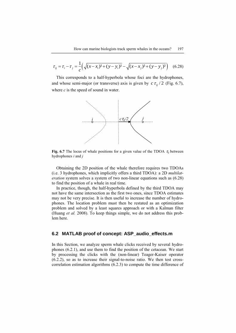
This corresponds to a half-hyperbola whose foci are the hydrophones,

and whose semi-major (or transverse) axis is given by / 2ijc (Fig. 6.7),

where c is the speed of sound in water.

Fig. 6.7 The locus of whale positions for a given value of the TDOA ij between

hydrophones i and j

Obtaining the 2D position of the whale therefore requires two TDOAs

(i.e. 3 hydrophones, which implicitly offers a third TDOA): a 2D multilat-

eration system solves a system of two non-linear equations such as (6.28)

to find the position of a whale in real time.

In practice, though, the half-hyperbola defined by the third TDOA may

not have the same intersection as the first two ones, since TDOA estimates

may not be very precise. It is then useful to increase the number of hydro-

phones. The location problem must then be restated as an optimization

problem and solved by a least squares approach or with a Kalman filter

(Huang et al. 2008). To keep things simple, we do not address this prob-

lem here.

6.2 MATLAB proof of concept: ASP_audio_effects.m

In this Section, we analyze sperm whale clicks received by several hydro-

phones (6.2.1), and use them to find the position of the cetacean. We start

by processing the clicks with the (non-linear) Teager-Kaiser operator

(6.2.2), so as to increase their signal-to-noise ratio. We then test cross-

correlation estimation algorithms (6.2.3) to compute the time difference of

i j cij/2


arrival (TDOA) between pairs of hydrophones, and compare them to an ef-

ficient adaptive estimation algorithm based on least means squares mini-

mization (6.2.4). We conclude by a simple multilateration algorithm,

which uses two TDOAs to estimate the position of the sperm whale

(6.2.5).

6.2.1 Sperm whale sounds

Throughout Section 6.2, we will work on hydrophone signals collected at

the Atlantic Undersea Test and Evaluation Center (AUTEC), Andros Is-

land, Bahamas, and made available by the Naval Undersea War-fare Cen-

ter (NUWC). These signals were provided to the 2nd International Work-

shop on Detection and Localization of Marine Mammals using Passive

Acoustics, held in Monaco November 16–18, 2005 (Adam et al. 2006) and

can be obtained from their website (Adam 2005). The Andros Island area

has over five hundred square nautical miles of ocean that are simultane-

ously monitored via 68 broad-band hydrophones. The distance between

most hydrophones is 5 nautical miles (about 7.5 km).

We will work with the sounds received by hydrophones I, G, and H

(which we will rename as #1, #2, and #3 here), for about 30 seconds, re-

corded with a digital audio recorder at Fs=48 kHz.

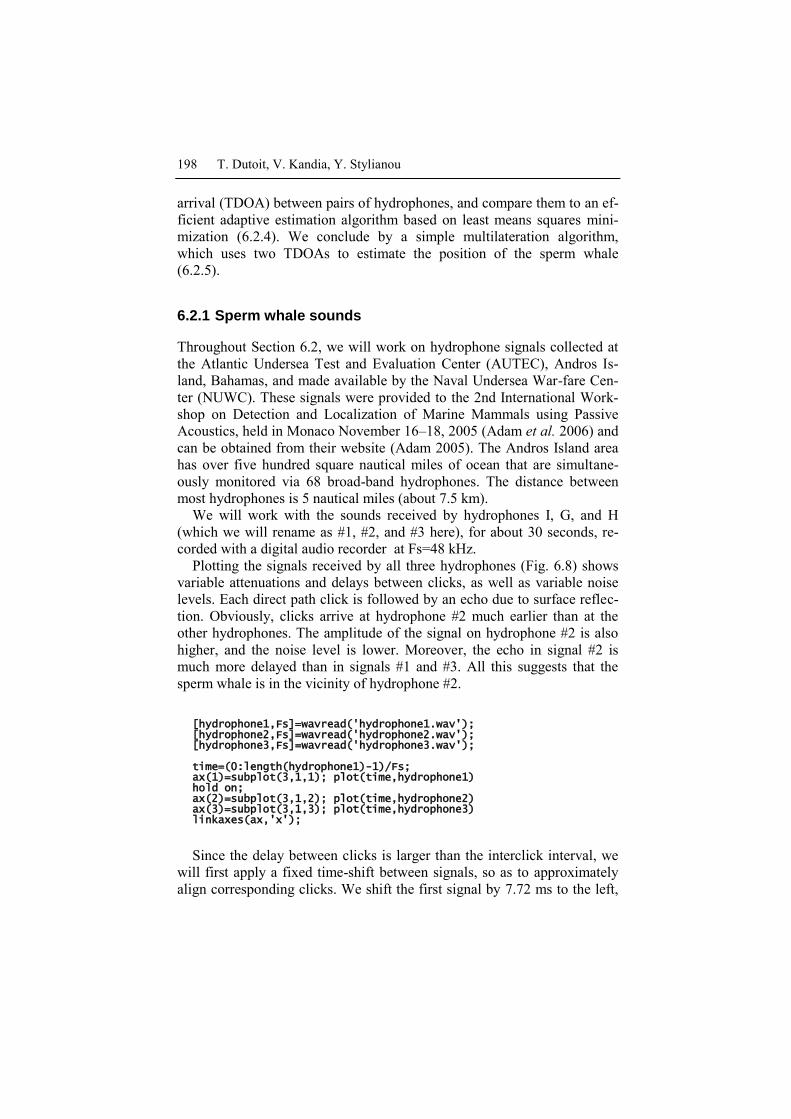
Plotting the signals received by all three hydrophones (Fig. 6.8) shows

variable attenuations and delays between clicks, as well as variable noise

levels. Each direct path click is followed by an echo due to surface reflec-

tion. Obviously, clicks arrive at hydrophone #2 much earlier than at the

other hydrophones. The amplitude of the signal on hydrophone #2 is also

higher, and the noise level is lower. Moreover, the echo in signal #2 is

much more delayed than in signals #1 and #3. All this suggests that the

sperm whale is in the vicinity of hydrophone #2.

[hydrophone1,Fs]=wavread('hydrophone1.wav'); [hydrophone2,Fs]=wavread('hydrophone2.wav'); [hydrophone3,Fs]=wavread('hydrophone3.wav'); time=(0:length(hydrophone1)-1)/Fs; ax(1)=subplot(3,1,1); plot(time,hydrophone1) hold on; ax(2)=subplot(3,1,2); plot(time,hydrophone2) ax(3)=subplot(3,1,3); plot(time,hydrophone3) linkaxes(ax,'x');

Since the delay between clicks is larger than the interclick interval, we

will first apply a fixed time-shift between signals, so as to approximately

align corresponding clicks. We shift the first signal by 7.72 ms to the left,


the second signal by 5.4 s to the left, third signal by 7.58 s to the left, and

keep 25 s of each signal. We will later account for these artificial shifts.

0 5 10 15 20 25 30 35-0.2

0

0.2

Am

plit

ude

hydrophone #1

0 5 10 15 20 25 30 35-1

0

1

Am

plit

ude

hydrophone #2

0 5 10 15 20 25 30 35-0.2

0

0.2

Time (s)

Am

plit

ude

hydrophone #3

0 5 10 15 20 25-0.2

0

0.2

Am

plit

ude

hydrophone #1

0 5 10 15 20 25-1

0

1

Am

plit

ude

hydrophone #2

0 5 10 15 20 25-0.2

0

0.2

Time (s)A

mplit

ude

hydrophone #3

Fig. 6.8 Left: Clicks received by hydrophones #1, #2, and #3. Echoes are clearly

visible between clicks (notice that the echo received at hydrophone #2 is more de-

layed than for the other hydrophones); Right: Same signals, time-shifted so as to

approximately align corresponding clicks.

n_samples=25*Fs; shift_1=fix(7.72*Fs); shift_2=fix(5.40*Fs); shift_3=fix(7.58*Fs); [hydrophone1,Fs]=wavread('hydrophone1.wav',[1+shift_1 ... shift_1+n_samples]); [hydrophone2,Fs]=wavread('hydrophone2.wav',[1+shift_2 ... shift_2+n_samples]); [hydrophone3,Fs]=wavread('hydrophone3.wav',[1+shift_3 ... shift_3+n_samples]);

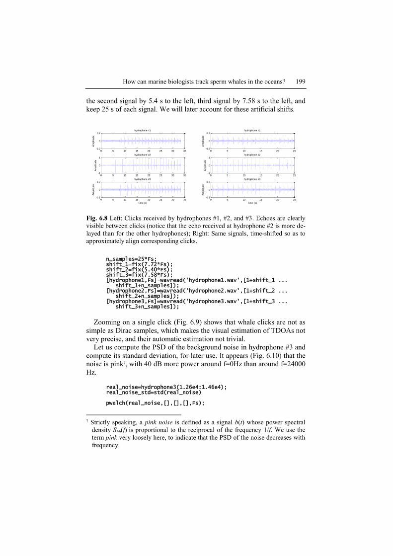
Zooming on a single click (Fig. 6.9) shows that whale clicks are not as

simple as Dirac samples, which makes the visual estimation of TDOAs not

very precise, and their automatic estimation not trivial.

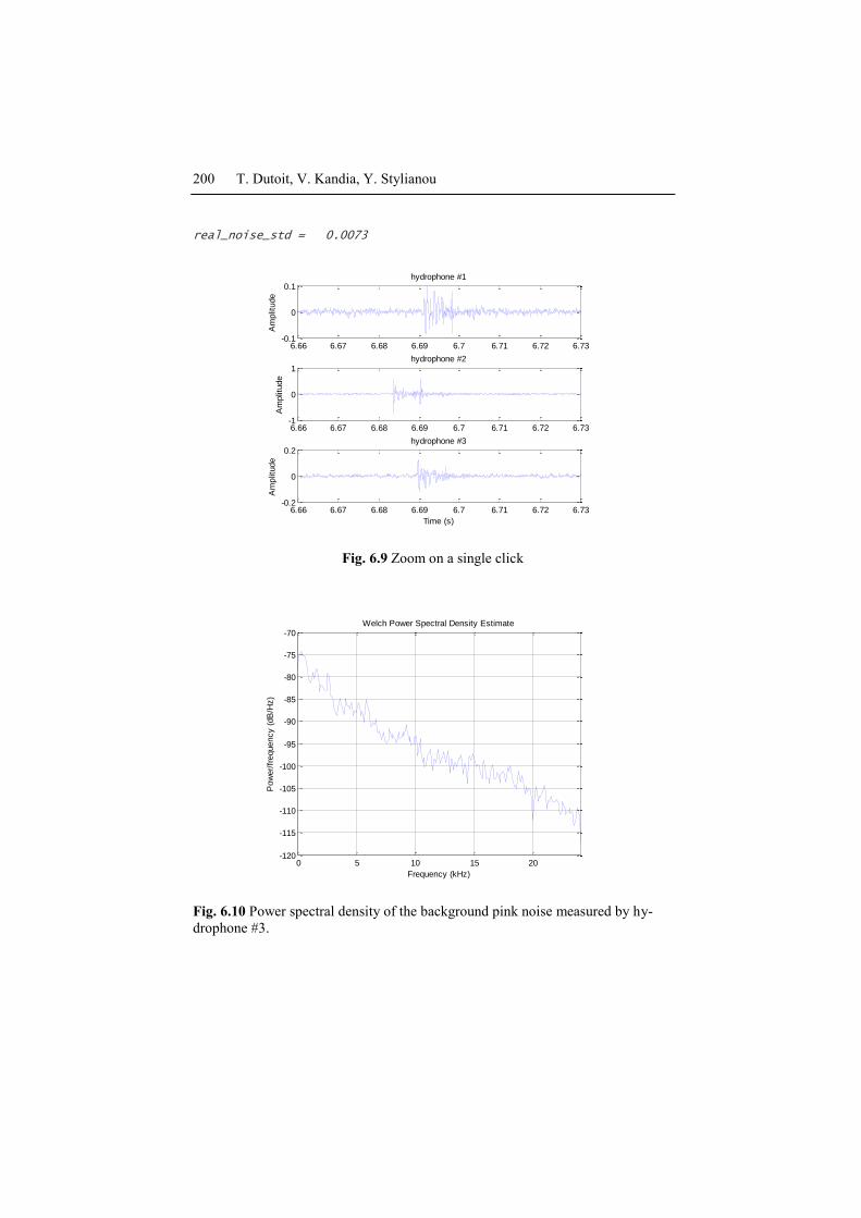
Let us compute the PSD of the background noise in hydrophone #3 and

compute its standard deviation, for later use. It appears (Fig. 6.10) that the

noise is pink7, with 40 dB more power around f=0Hz than around f=24000

Hz.

real_noise=hydrophone3(1.26e4:1.46e4); real_noise_std=std(real_noise) pwelch(real_noise,[],[],[],Fs);

7 Strictly speaking, a pink noise is defined as a signal b(t) whose power spectral

density Sbb(f) is proportional to the reciprocal of the frequency 1/f. We use the

term pink very loosely here, to indicate that the PSD of the noise decreases with

frequency.

http://en.wikipedia.org/wiki/Signal_%28information_theory%29

http://en.wikipedia.org/wiki/Spectral_density




real_noise_std = 0.0073

6.66 6.67 6.68 6.69 6.7 6.71 6.72 6.73-0.1

0

0.1

Am

plit

ude

hydrophone #1

6.66 6.67 6.68 6.69 6.7 6.71 6.72 6.73-1

0

1

Am

plit

ude

hydrophone #2

6.66 6.67 6.68 6.69 6.7 6.71 6.72 6.73-0.2

0

0.2

Time (s)

Am

plit

ude

hydrophone #3

Fig. 6.9 Zoom on a single click

0 5 10 15 20-120

-115

-110

-105

-100

-95

-90

-85

-80

-75

-70

Frequency (kHz)

Pow

er/

frequency (

dB

/Hz)

Welch Power Spectral Density Estimate

Fig. 6.10 Power spectral density of the background pink noise measured by hy-

drophone #3.


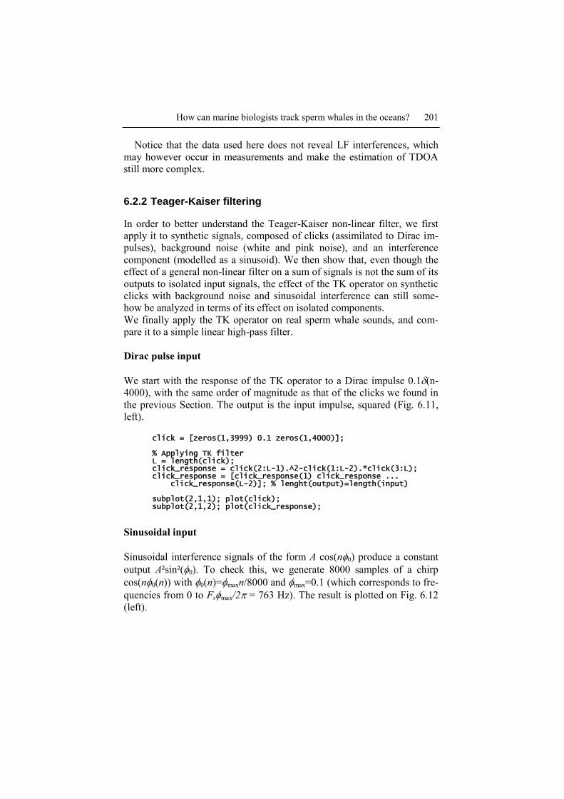
Notice that the data used here does not reveal LF interferences, which

may however occur in measurements and make the estimation of TDOA

still more complex.

6.2.2 Teager-Kaiser filtering

In order to better understand the Teager-Kaiser non-linear filter, we first

apply it to synthetic signals, composed of clicks (assimilated to Dirac im-

pulses), background noise (white and pink noise), and an interference

component (modelled as a sinusoid). We then show that, even though the

effect of a general non-linear filter on a sum of signals is not the sum of its

outputs to isolated input signals, the effect of the TK operator on synthetic

clicks with background noise and sinusoidal interference can still some-

how be analyzed in terms of its effect on isolated components.

We finally apply the TK operator on real sperm whale sounds, and com-

pare it to a simple linear high-pass filter.

Dirac pulse input

We start with the response of the TK operator to a Dirac impulse 0.1(n-

4000), with the same order of magnitude as that of the clicks we found in

the previous Section. The output is the input impulse, squared (Fig. 6.11,

left).

click = [zeros(1,3999) 0.1 zeros(1,4000)]; % Applying TK filter L = length(click); click_response = click(2:L-1).^2-click(1:L-2).*click(3:L); click_response = [click_response(1) click_response ... click_response(L-2)]; % lenght(output)=length(input) subplot(2,1,1); plot(click); subplot(2,1,2); plot(click_response);

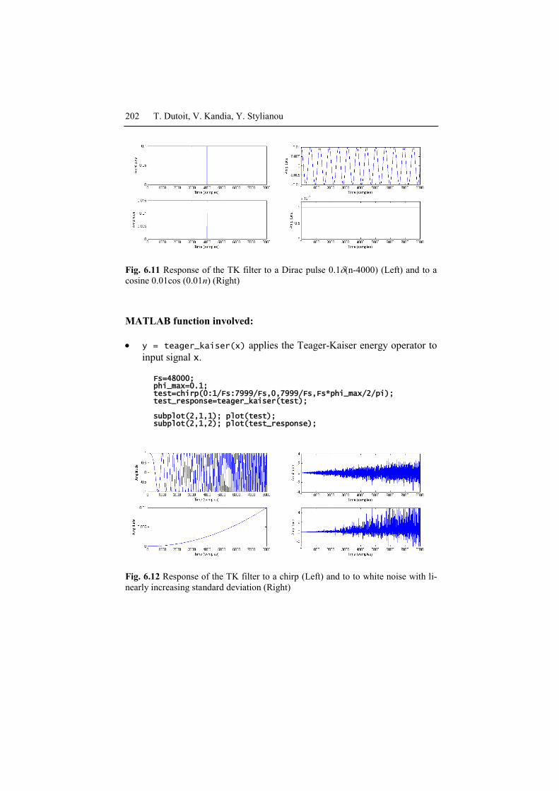
Sinusoidal input

Sinusoidal interference signals of the form A cos(n0) produce a constant

output A²sin²(0). To check this, we generate 8000 samples of a chirp

cos(n0(n)) with 0(n)=maxn/8000 and max=0.1 (which corresponds to fre-

quencies from 0 to Fsmax/2 = 763 Hz). The result is plotted on Fig. 6.12

(left).


Fig. 6.11 Response of the TK filter to a Dirac pulse 0.1(n-4000) (Left) and to a

cosine 0.01cos (0.01n) (Right)

MATLAB function involved:

y = teager_kaiser(x) applies the Teager-Kaiser energy operator to

input signal x.

Fs=48000; phi_max=0.1; test=chirp(0:1/Fs:7999/Fs,0,7999/Fs,Fs*phi_max/2/pi); test_response=teager_kaiser(test); subplot(2,1,1); plot(test); subplot(2,1,2); plot(test_response);

Fig. 6.12 Response of the TK filter to a chirp (Left) and to to white noise with li-

nearly increasing standard deviation (Right)


The value of the output is close to zero when 0 is small, which will be

the case for a typical LF interference component in sperm whale click

measurements (Fig. 6.11, right).

interference = 0.01*cos (0.01*(0:7999)); % A²sin²(0.01)~1e-8 interference_response=teager_kaiser(interference); subplot(2,1,1); plot(interference); subplot(2,1,2); plot(interference_response);

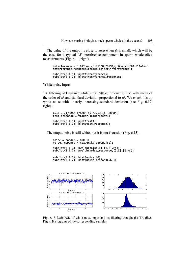
White noise input

TK filtering of Gaussian white noise N(0,) produces noise with mean of

the order of ² and standard deviation proportional to ². We check this on

white noise with linearly increasing standard deviation (see Fig. 6.12,

right).

test = (1/8000:1/8000:1).*randn(1, 8000); test_response = teager_kaiser(test); subplot(2,1,1); plot(test); subplot(2,1,2); plot(test_response);

The output noise is still white, but it is not Gaussian (Fig. 6.13).

noise = randn(1, 8000); noise_response = teager_kaiser(noise); subplot(2,1,1); pwelch(noise,[],[],[],Fs); subplot(2,1,2); pwelch(noise_response,[],[],[],Fs);

subplot(2,1,1); hist(noise,30); subplot(2,1,2); hist(noise_response,60);

Fig. 6.13 Left: PSD of white noise input and its filtering thought the TK filter;

Right: Histograms of the corresponding samples


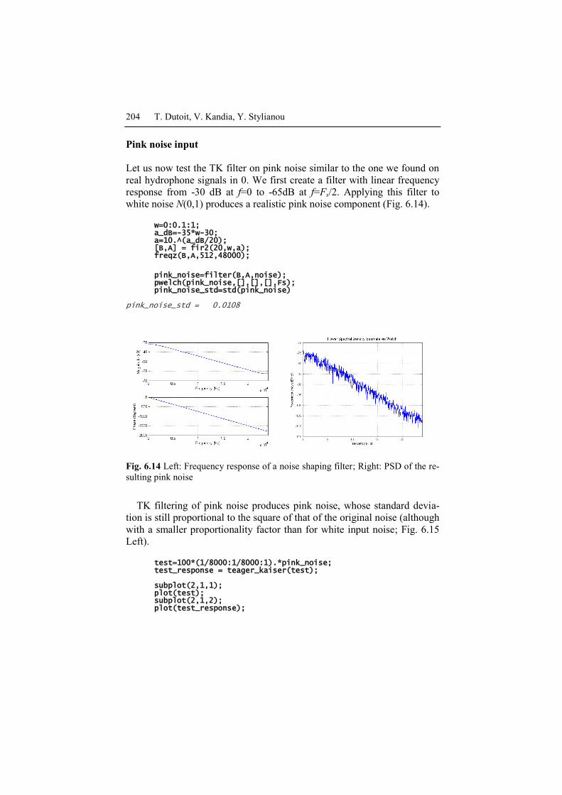
Pink noise input

Let us now test the TK filter on pink noise similar to the one we found on

real hydrophone signals in 0. We first create a filter with linear frequency

response from -30 dB at f=0 to -65dB at f=Fs/2. Applying this filter to

white noise N(0,1) produces a realistic pink noise component (Fig. 6.14).

w=0:0.1:1; a_dB=-35*w-30; a=10.^(a_dB/20); [B,A] = fir2(20,w,a); freqz(B,A,512,48000);

pink_noise=filter(B,A,noise); pwelch(pink_noise,[],[],[],Fs); pink_noise_std=std(pink_noise)

pink_noise_std = 0.0108

Fig. 6.14 Left: Frequency response of a noise shaping filter; Right: PSD of the re-

sulting pink noise

TK filtering of pink noise produces pink noise, whose standard devia-

tion is still proportional to the square of that of the original noise (although

with a smaller proportionality factor than for white input noise; Fig. 6.15

Left).

test=100*(1/8000:1/8000:1).*pink_noise; test_response = teager_kaiser(test); subplot(2,1,1); plot(test); subplot(2,1,2); plot(test_response);


The output noise is whiter; the PSD of the input noise has been de-

creased by about 50 dB in low frequencies and by about 30 dB in high fre-

quencies (Fig. 6.15 Right).

pink_noise_response = teager_kaiser(pink_noise); subplot(2,1,1); pwelch(pink_noise,[],[],[],Fs); subplot(2,1,2); pwelch(pink_noise_response,[],[],[],Fs);

Fig. 6.15 Left: TK filtering of pink noise with linearly increasing standard devia-

tion; Right: PSDs of input pink noise (with constant variance) and of its filtering

through the TK filter.

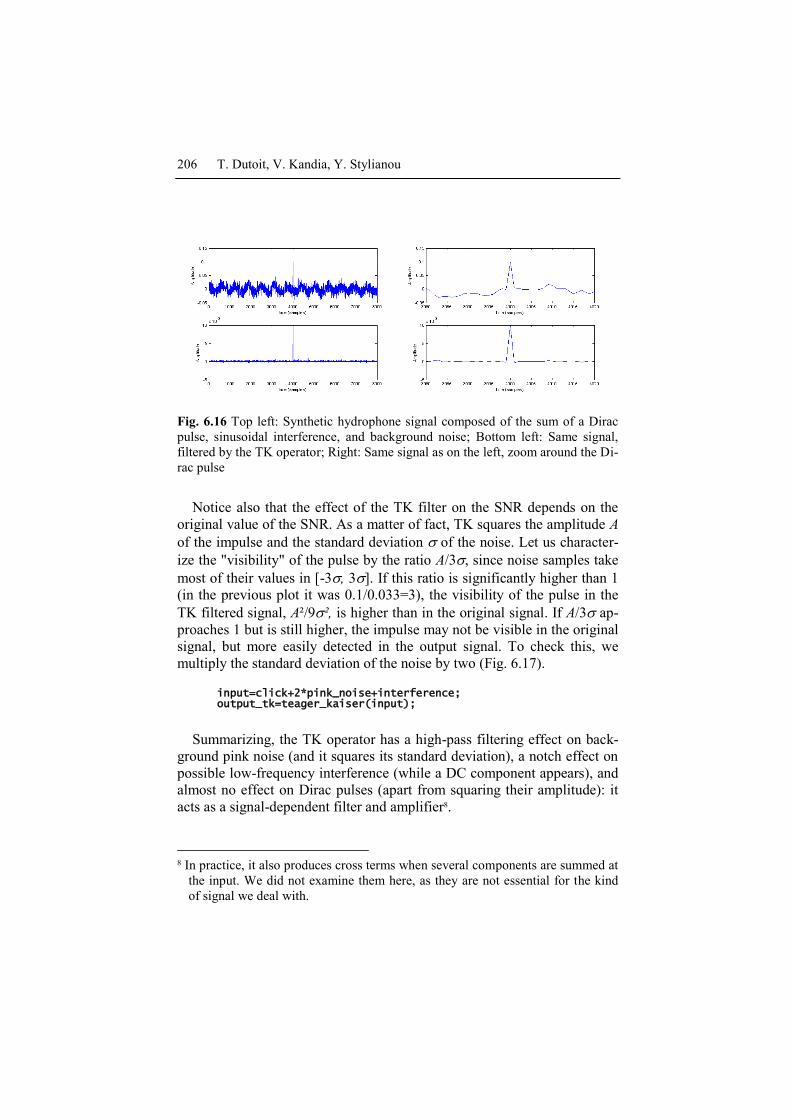
Complex input

We now apply the TK operator to the complete synthetic signal, obtained

by summing all three components: click, interference, and pink noise (Fig.

6.16, left). Thanks to the TK operator, the impulse is highlighted in the

signal. The LF signal is removed, and the pink noise is very much attenu-

ated relatively to the impulse. The SNR is therefore highly increased.

input=click+interference+pink_noise; output_tk=teager_kaiser(input); subplot(2,1,1); plot(input); subplot(2,1,2); plot(output_tk);

Notice that the TK operator did not smear the impulsive part of the input

waveform (Fig. 6.16, right).

set(gca,'xlim',[3980 4020]);


Fig. 6.16 Top left: Synthetic hydrophone signal composed of the sum of a Dirac

pulse, sinusoidal interference, and background noise; Bottom left: Same signal,

filtered by the TK operator; Right: Same signal as on the left, zoom around the Di-

rac pulse

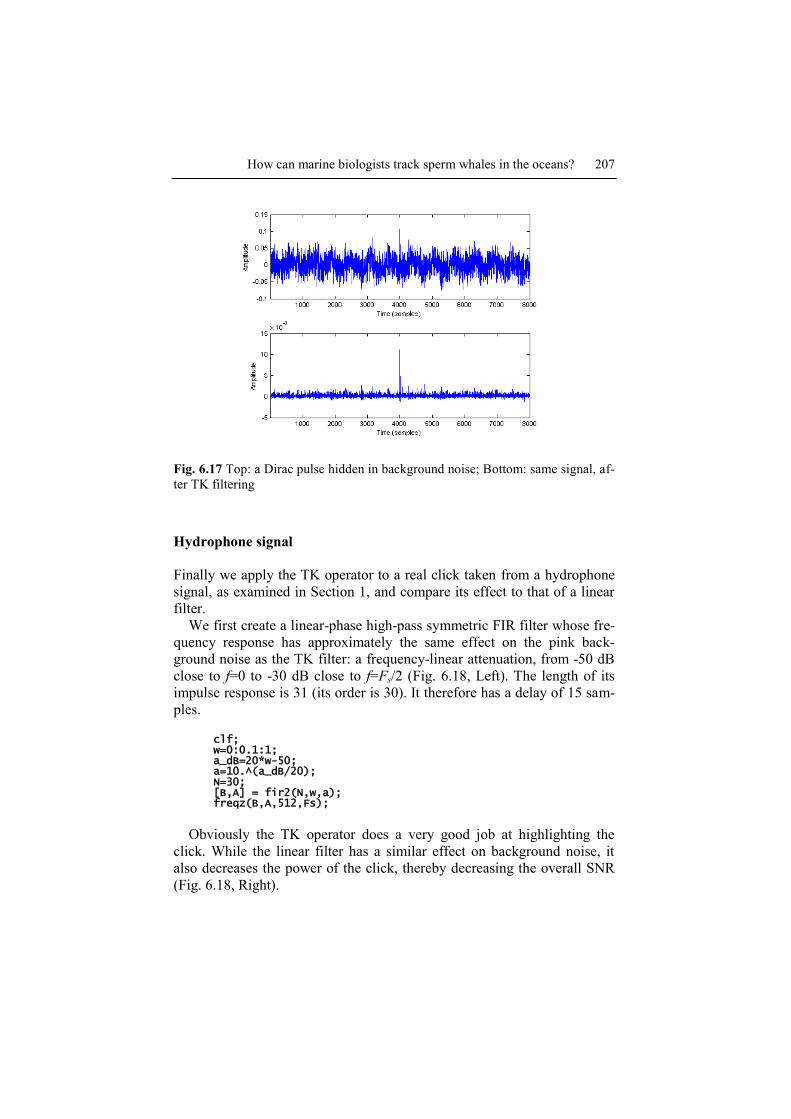
Notice also that the effect of the TK filter on the SNR depends on the

original value of the SNR. As a matter of fact, TK squares the amplitude A

of the impulse and the standard deviation of the noise. Let us character-

ize the "visibility" of the pulse by the ratio A/3, since noise samples take

most of their values in [-3, 3]. If this ratio is significantly higher than 1

(in the previous plot it was 0.1/0.033=3), the visibility of the pulse in the

TK filtered signal, A²/9², is higher than in the original signal. If A/3 ap-

proaches 1 but is still higher, the impulse may not be visible in the original

signal, but more easily detected in the output signal. To check this, we

multiply the standard deviation of the noise by two (Fig. 6.17).

input=click+2*pink_noise+interference; output_tk=teager_kaiser(input);

Summarizing, the TK operator has a high-pass filtering effect on back-

ground pink noise (and it squares its standard deviation), a notch effect on

possible low-frequency interference (while a DC component appears), and

almost no effect on Dirac pulses (apart from squaring their amplitude): it

acts as a signal-dependent filter and amplifier8.

8 In practice, it also produces cross terms when several components are summed at

the input. We did not examine them here, as they are not essential for the kind

of signal we deal with.


Fig. 6.17 Top: a Dirac pulse hidden in background noise; Bottom: same signal, af-

ter TK filtering

Hydrophone signal

Finally we apply the TK operator to a real click taken from a hydrophone

signal, as examined in Section 1, and compare its effect to that of a linear

filter.

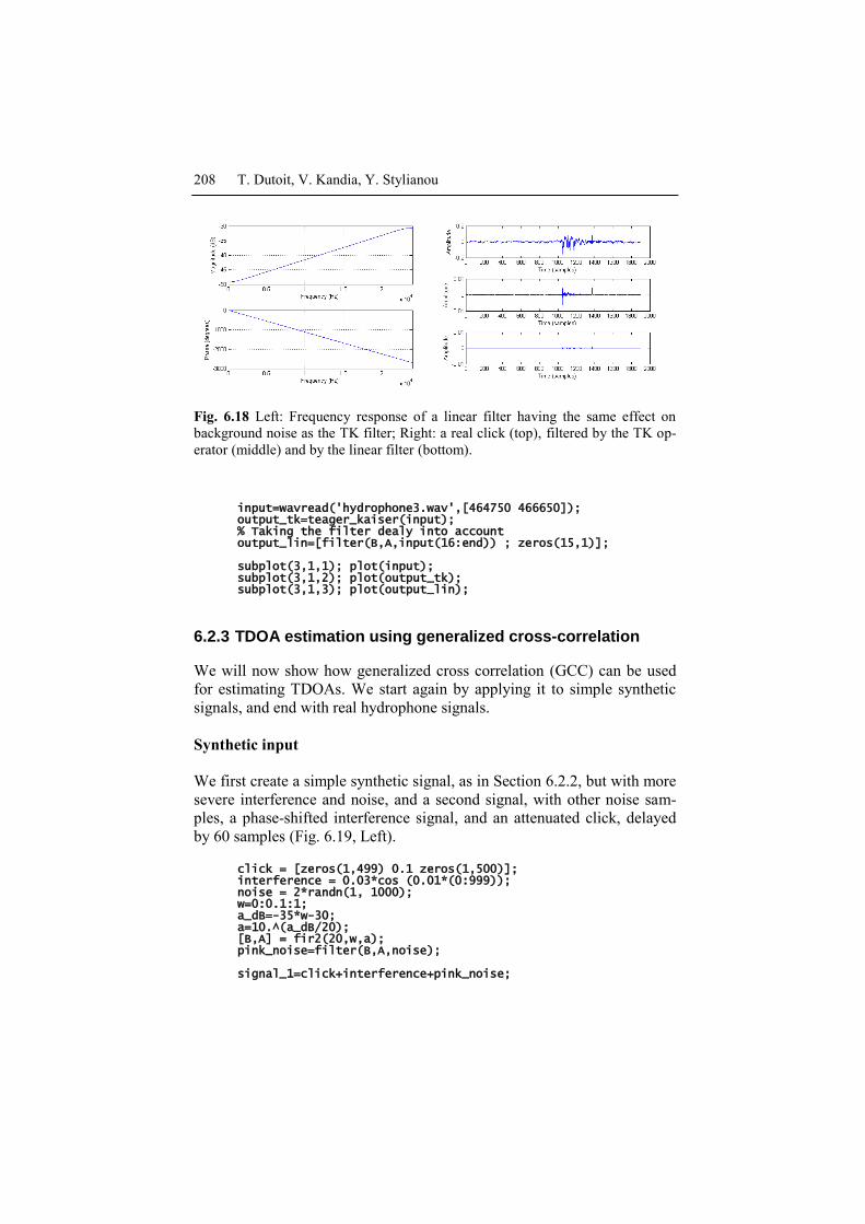
We first create a linear-phase high-pass symmetric FIR filter whose fre-

quency response has approximately the same effect on the pink back-

ground noise as the TK filter: a frequency-linear attenuation, from -50 dB

close to f=0 to -30 dB close to f=Fs/2 (Fig. 6.18, Left). The length of its

impulse response is 31 (its order is 30). It therefore has a delay of 15 sam-

ples.

clf; w=0:0.1:1; a_dB=20*w-50; a=10.^(a_dB/20); N=30; [B,A] = fir2(N,w,a); freqz(B,A,512,Fs);

Obviously the TK operator does a very good job at highlighting the

click. While the linear filter has a similar effect on background noise, it

also decreases the power of the click, thereby decreasing the overall SNR

(Fig. 6.18, Right).


Fig. 6.18 Left: Frequency response of a linear filter having the same effect on

background noise as the TK filter; Right: a real click (top), filtered by the TK op-

erator (middle) and by the linear filter (bottom).

input=wavread('hydrophone3.wav',[464750 466650]); output_tk=teager_kaiser(input); % Taking the filter dealy into account output_lin=[filter(B,A,input(16:end)) ; zeros(15,1)]; subplot(3,1,1); plot(input); subplot(3,1,2); plot(output_tk); subplot(3,1,3); plot(output_lin);

6.2.3 TDOA estimation using generalized cross-correlation

We will now show how generalized cross correlation (GCC) can be used

for estimating TDOAs. We start again by applying it to simple synthetic

signals, and end with real hydrophone signals.

Synthetic input

We first create a simple synthetic signal, as in Section 6.2.2, but with more

severe interference and noise, and a second signal, with other noise sam-

ples, a phase-shifted interference signal, and an attenuated click, delayed

by 60 samples (Fig. 6.19, Left).

click = [zeros(1,499) 0.1 zeros(1,500)]; interference = 0.03*cos (0.01*(0:999)); noise = 2*randn(1, 1000); w=0:0.1:1; a_dB=-35*w-30; a=10.^(a_dB/20); [B,A] = fir2(20,w,a); pink_noise=filter(B,A,noise); signal_1=click+interference+pink_noise;


click_2=circshift(click'*0.5,60)'; interference_2 = 0.02*cos (pi/4+0.01*(0:999)); noise_2 = randn(1, 1000); % new noise samples pink_noise_2=filter(B,A,noise_2); signal_2=click_2+interference_2+pink_noise_2; subplot(2,1,1); plot(signal_1); subplot(2,1,2); plot(signal_2);

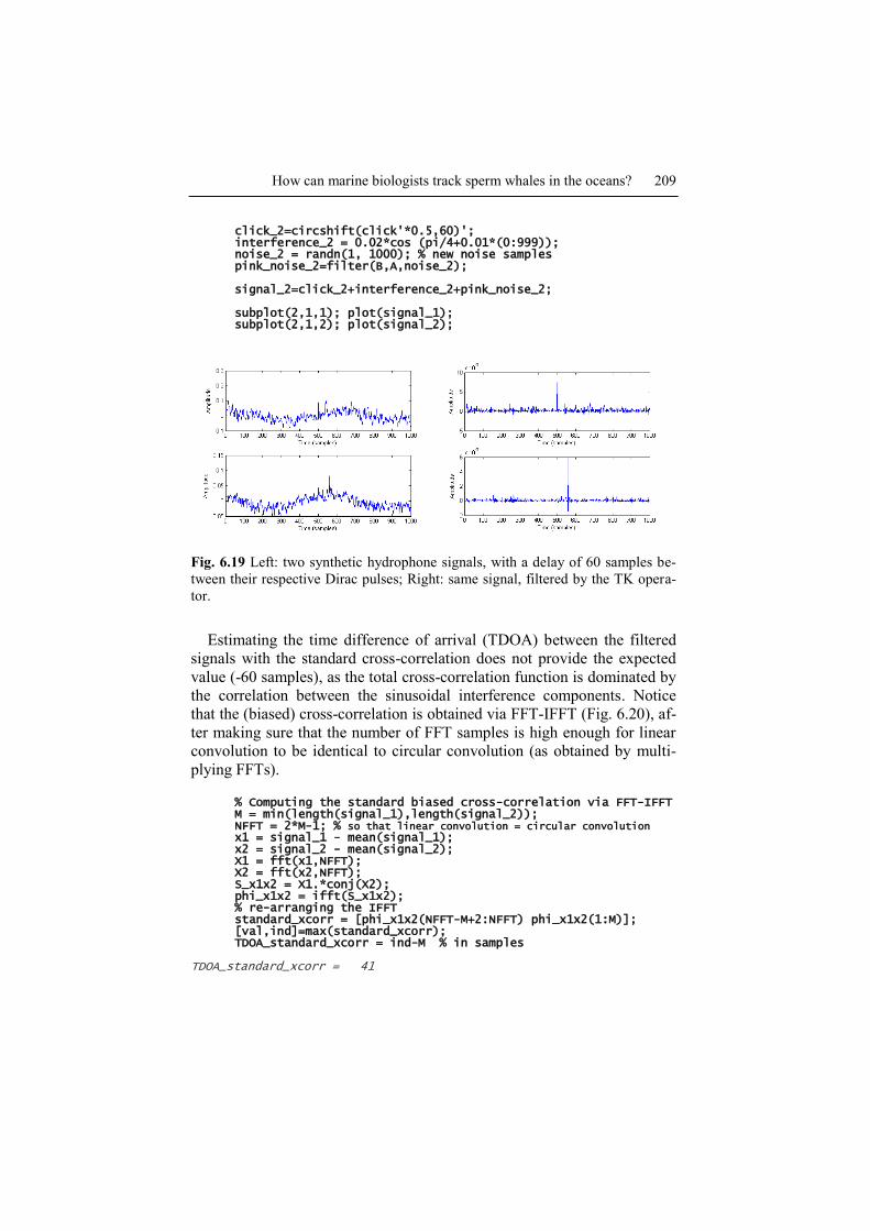
Fig. 6.19 Left: two synthetic hydrophone signals, with a delay of 60 samples be-

tween their respective Dirac pulses; Right: same signal, filtered by the TK opera-

tor.

Estimating the time difference of arrival (TDOA) between the filtered

signals with the standard cross-correlation does not provide the expected

value (-60 samples), as the total cross-correlation function is dominated by

the correlation between the sinusoidal interference components. Notice

that the (biased) cross-correlation is obtained via FFT-IFFT (Fig. 6.20), af-

ter making sure that the number of FFT samples is high enough for linear

convolution to be identical to circular convolution (as obtained by multi-

plying FFTs).

% Computing the standard biased cross-correlation via FFT-IFFT M = min(length(signal_1),length(signal_2)); NFFT = 2*M-1; % so that linear convolution = circular convolution x1 = signal_1 - mean(signal_1); x2 = signal_2 - mean(signal_2); X1 = fft(x1,NFFT); X2 = fft(x2,NFFT); S_x1x2 = X1.*conj(X2); phi_x1x2 = ifft(S_x1x2); % re-arranging the IFFT standard_xcorr = [phi_x1x2(NFFT-M+2:NFFT) phi_x1x2(1:M)]; [val,ind]=max(standard_xcorr); TDOA_standard_xcorr = ind-M % in samples

TDOA_standard_xcorr = 41


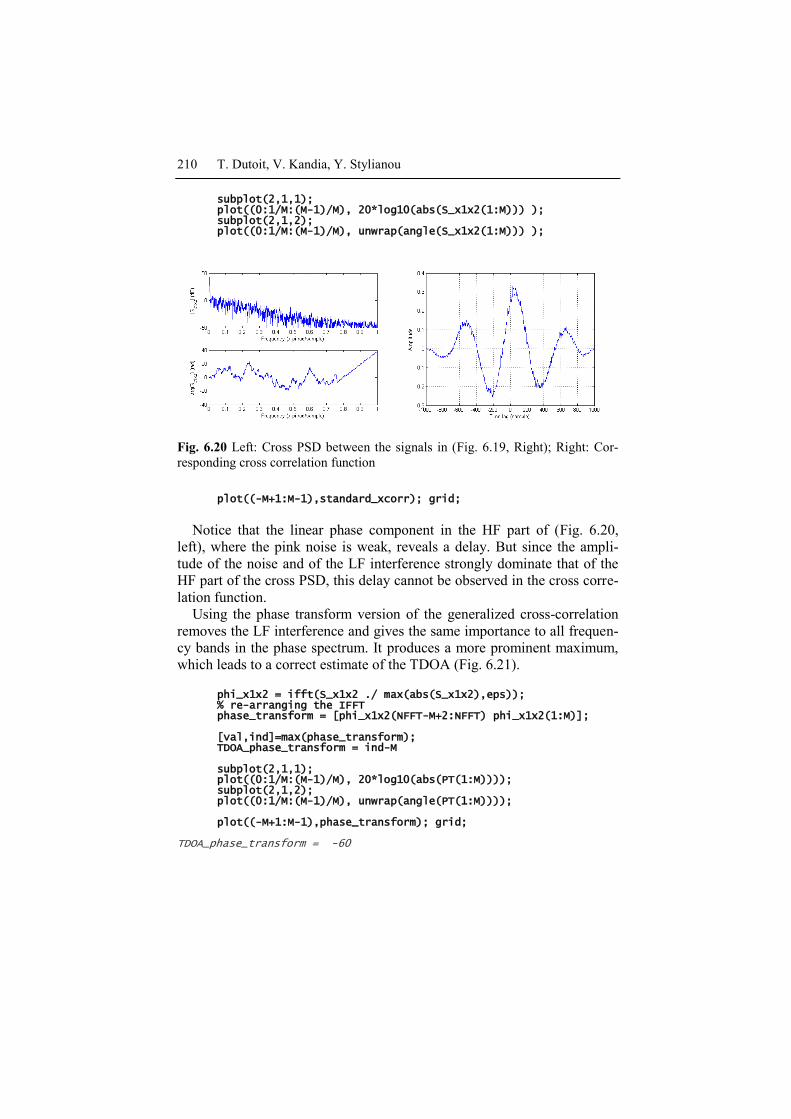
subplot(2,1,1); plot((0:1/M:(M-1)/M), 20*log10(abs(S_x1x2(1:M))) ); subplot(2,1,2); plot((0:1/M:(M-1)/M), unwrap(angle(S_x1x2(1:M))) );

Fig. 6.20 Left: Cross PSD between the signals in (Fig. 6.19, Right); Right: Cor-

responding cross correlation function

plot((-M+1:M-1),standard_xcorr); grid;

Notice that the linear phase component in the HF part of (Fig. 6.20,

left), where the pink noise is weak, reveals a delay. But since the ampli-

tude of the noise and of the LF interference strongly dominate that of the

HF part of the cross PSD, this delay cannot be observed in the cross corre-

lation function.

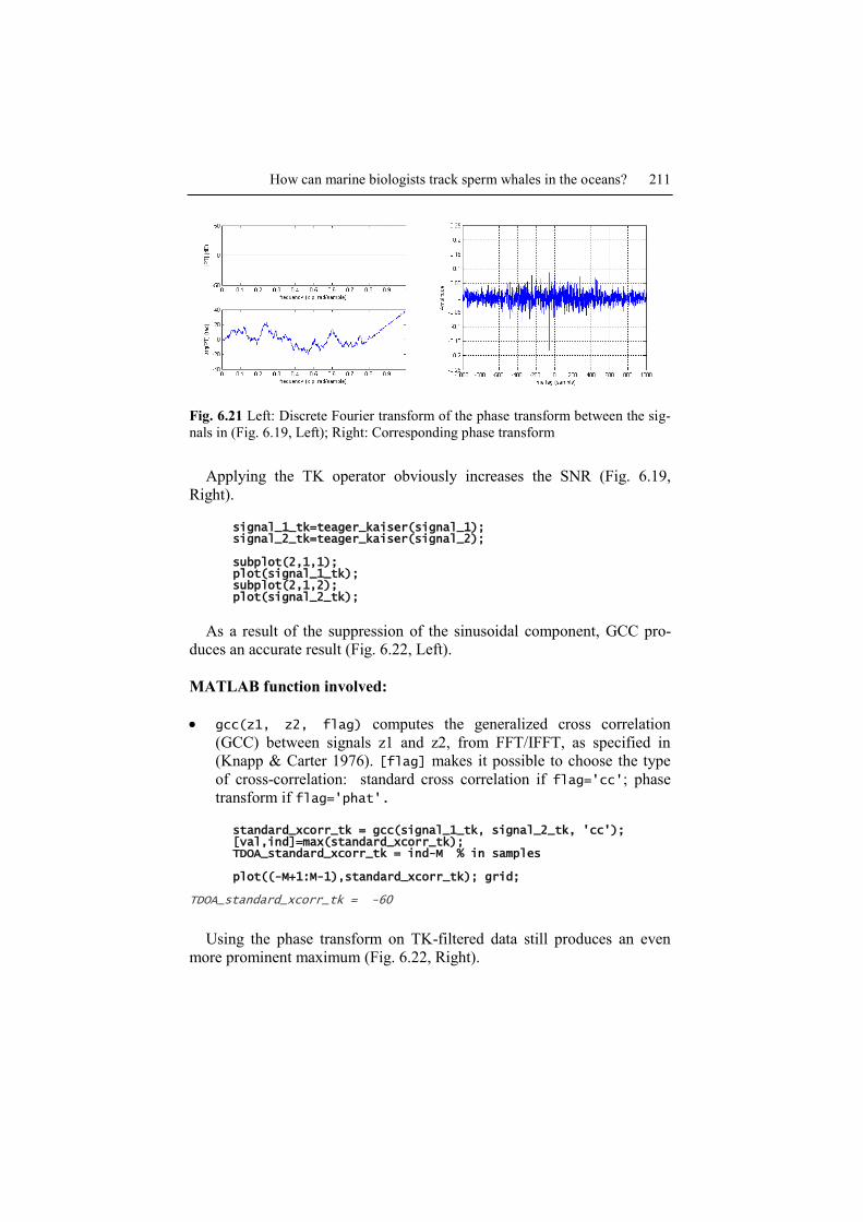
Using the phase transform version of the generalized cross-correlation

removes the LF interference and gives the same importance to all frequen-

cy bands in the phase spectrum. It produces a more prominent maximum,

which leads to a correct estimate of the TDOA (Fig. 6.21).

phi_x1x2 = ifft(S_x1x2 ./ max(abs(S_x1x2),eps)); % re-arranging the IFFT phase_transform = [phi_x1x2(NFFT-M+2:NFFT) phi_x1x2(1:M)]; [val,ind]=max(phase_transform); TDOA_phase_transform = ind-M subplot(2,1,1); plot((0:1/M:(M-1)/M), 20*log10(abs(PT(1:M)))); subplot(2,1,2); plot((0:1/M:(M-1)/M), unwrap(angle(PT(1:M)))); plot((-M+1:M-1),phase_transform); grid;

TDOA_phase_transform = -60


Fig. 6.21 Left: Discrete Fourier transform of the phase transform between the sig-

nals in (Fig. 6.19, Left); Right: Corresponding phase transform

Applying the TK operator obviously increases the SNR (Fig. 6.19,

Right).

signal_1_tk=teager_kaiser(signal_1); signal_2_tk=teager_kaiser(signal_2); subplot(2,1,1); plot(signal_1_tk); subplot(2,1,2); plot(signal_2_tk);

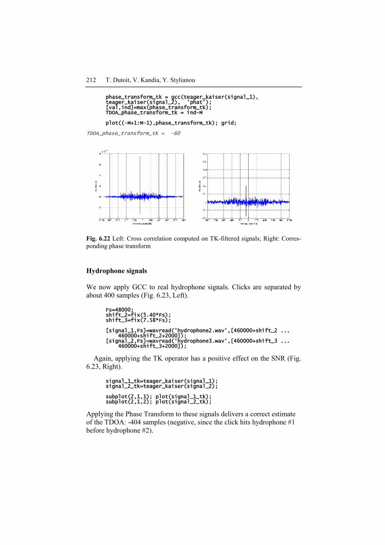
As a result of the suppression of the sinusoidal component, GCC pro-

duces an accurate result (Fig. 6.22, Left).


gcc(z1, z2, flag) computes the generalized cross correlation

(GCC) between signals z1 and z2, from FFT/IFFT, as specified in

(Knapp & Carter 1976). [flag] makes it possible to choose the type

of cross-correlation: standard cross correlation if flag='cc'; phase

transform if flag='phat'.

standard_xcorr_tk = gcc(signal_1_tk, signal_2_tk, 'cc'); [val,ind]=max(standard_xcorr_tk); TDOA_standard_xcorr_tk = ind-M % in samples plot((-M+1:M-1),standard_xcorr_tk); grid;

TDOA_standard_xcorr_tk = -60

Using the phase transform on TK-filtered data still produces an even

more prominent maximum (Fig. 6.22, Right).


phase_transform_tk = gcc(teager_kaiser(signal_1), teager_kaiser(signal_2), 'phat'); [val,ind]=max(phase_transform_tk); TDOA_phase_transform_tk = ind-M plot((-M+1:M-1),phase_transform_tk); grid;

TDOA_phase_transform_tk = -60

Fig. 6.22 Left: Cross correlation computed on TK-filtered signals; Right: Corres-

ponding phase transform

Hydrophone signals

We now apply GCC to real hydrophone signals. Clicks are separated by

about 400 samples (Fig. 6.23, Left).

Fs=48000; shift_2=fix(5.40*Fs); shift_3=fix(7.58*Fs); [signal_1,Fs]=wavread('hydrophone2.wav',[460000+shift_2 ... 460000+shift_2+2000]); [signal_2,Fs]=wavread('hydrophone3.wav',[460000+shift_3 ... 460000+shift_3+2000]);

Again, applying the TK operator has a positive effect on the SNR (Fig.

6.23, Right).

signal_1_tk=teager_kaiser(signal_1); signal_2_tk=teager_kaiser(signal_2); subplot(2,1,1); plot(signal_1_tk); subplot(2,1,2); plot(signal_2_tk);

Applying the Phase Transform to these signals delivers a correct estimate

of the TDOA: -404 samples (negative, since the click hits hydrophone #1

before hydrophone #2).


0 500 1000 1500 2000 2500-1

-0.5

0

0.5

1

Am

plit

ude

0 500 1000 1500 2000 2500-0.2

-0.1

0

0.1

0.2

Time (samples)

Am

plit

ude

0 500 1000 1500 2000 2500-0.5

0

0.5

Time (samples)

Am

plit

ude

0 500 1000 1500 2000 2500-5

0

5

10

15x 10

-3

Time (samples)

Am

plit

ude

Fig. 6.23 Left: Two clicks, showing a delay of about 400 samples. Right: same,

after TK filtering.

phase_transform_tk = gcc(signal_1_tk, signal_2_tk, 'phat'); [val,ind]=max(phase_transform_tk ); M = min(length(signal_1),length(signal_2)); TDOA_phase_transform_tk= ind-M

TDOA_phase_transform_tk = -404

6.2.4 TDOA estimation using least-mean squares

In this section we will apply the Least Mean Squares (LMS) adaptive ap-

proach to TDOA estimation, again first on synthetic signals (with imposed

TDOA), and then on real hydrophone signals.

Synthetic input

We start with the same synthetic signals as in Fig. 6.19, apply TK prepro-

cessing, and run the Benesty's adaptive filtering algorithm for TDOA esti-

mation within [-600,600] (samples) and step mu=0.01 (for full scale signals

in [-1,+1]).

load synthetic_signals signal_1 signal_2 signal_1_tk=teager_kaiser(signal_1); signal_2_tk=teager_kaiser(signal_2); % Normalizing max signal amplitudes to +1 x1=signal_1_tk/max(signal_1_tk); x2=signal_2_tk/max(signal_2_tk); % LMS initialization M = 600; % max value of the estimated TDOA x1c = zeros(M,1); x2c = zeros(M,1); u = zeros(2*M,1);


u(M/2) = 1; N = length(x1); e = zeros(1,N); tdoa = zeros(1,N); peak = zeros(1,N); mu = 0.01; % LMS step % LMS loop for n=1:N x1c = [x1(n);x1c(1:length(x1c)-1)]; x2c = [x2(n);x2c(1:length(x2c)-1)]; x = [x1c;x2c]; e(n) = u'*x; u = u-mu*e(n)*x; u(M/2) = 1; %forcing g2 to an impulse response at M/2 u = u/norm(u); %forcing ||u|| to 1 [peak(n),ind] = min(u(M+1:end)); peak(n)=-peak(n); % (positive) impulse in g1 TDOA(n) = ind-M/2; end % Estimated TDOA(n), with values of the maximum peak in g1 subplot(2,1,1); plot(TDOA); xlabel('Time (samples)'); ylabel('TDOA (samples)'); subplot(2,1,2); plot(peak); xlabel('Time (samples)'); ylabel('peak');

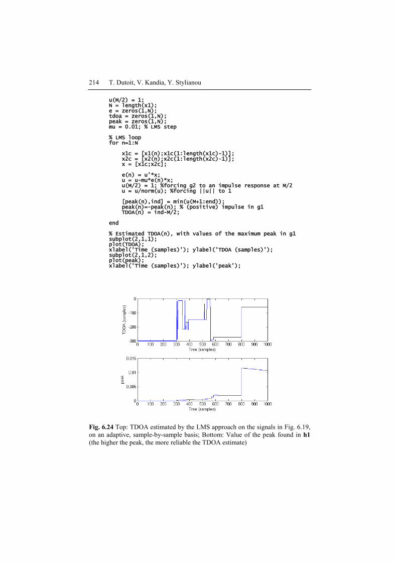
Fig. 6.24 Top: TDOA estimated by the LMS approach on the signals in Fig. 6.19,

on an adaptive, sample-by-sample basis; Bottom: Value of the peak found in h1

(the higher the peak, the more reliable the TDOA estimate)


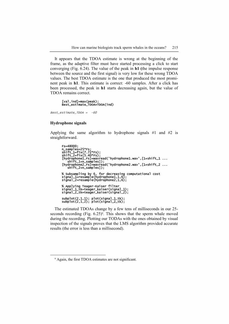
It appears that the TDOA estimate is wrong at the beginning of the

frame, as the adaptive filter must have started processing a click to start

converging (Fig. 6.24). The value of the peak in h1 (the impulse response

between the source and the first signal) is very low for these wrong TDOA

values. The best TDOA estimate is the one that produced the most promi-

nent peak in h1. This estimate is correct: -60 samples. After a click has

been processed, the peak in h1 starts decreasing again, but the value of

TDOA remains correct.

[val,ind]=max(peak); Best_estimate_TDOA=TDOA(ind)

Best_estimate_TDOA = -60

Hydrophone signals

Applying the same algorithm to hydrophone signals #1 and #2 is

straightforward.

Fs=48000; n_samples=25*Fs; shift_1=fix(7.72*Fs); shift_2=fix(5.40*Fs); [hydrophone1,Fs]=wavread('hydrophone1.wav',[1+shift_1 ... shift_1+n_samples]); [hydrophone2,Fs]=wavread('hydrophone2.wav',[1+shift_2 ... shift_2+n_samples]); % Subsampling by 6, for decreasing computational cost signal_1=resample(hydrophone1,1,6); signal_2=resample(hydrophone2,1,6); % Applying Teager-Kaiser filter signal_1_tk=teager_kaiser(signal_1); signal_2_tk=teager_kaiser(signal_2); subplot(2,1,1); plot(signal_1_tk); subplot(2,1,2); plot(signal_2_tk);

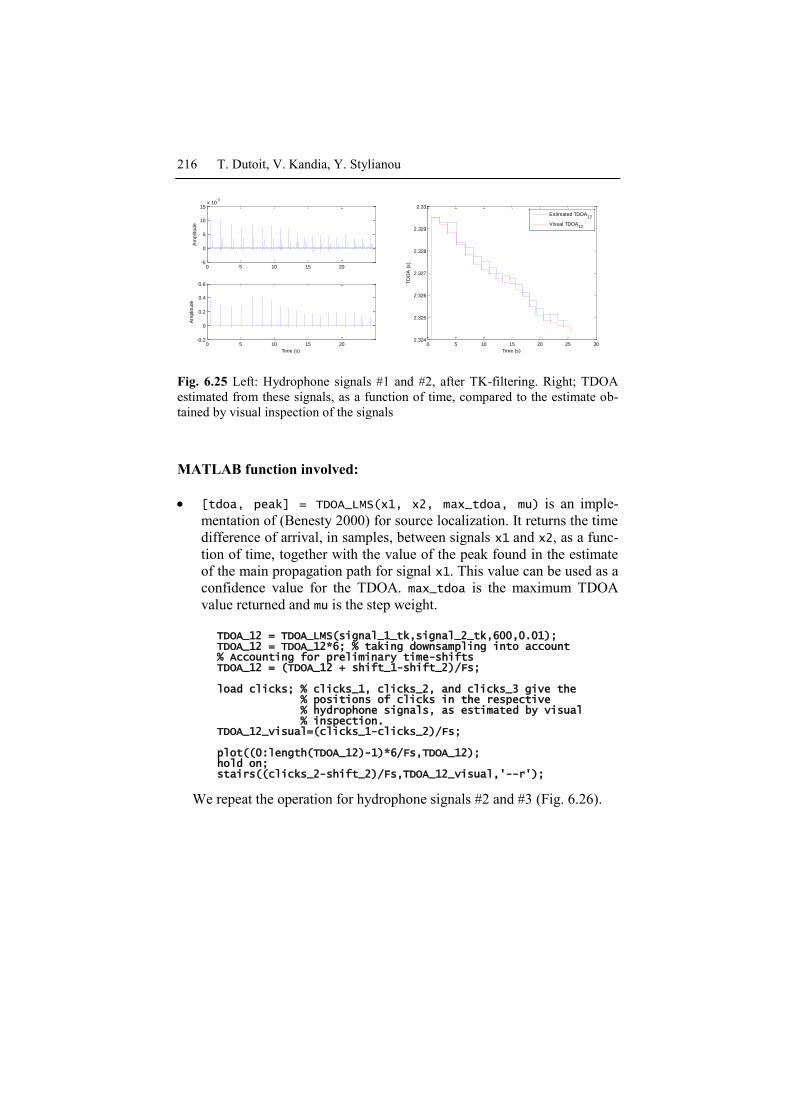
The estimated TDOAs change by a few tens of milliseconds in our 25-

seconds recording (Fig. 6.25)9. This shows that the sperm whale moved

during the recording. Plotting our TODAs with the ones obtained by visual

inspection of the signals proves that the LMS algorithm provided accurate

results (the error is less than a millisecond).

9 Again, the first TDOA estimates are not significant.


0 5 10 15 20-5

0

5

10

15x 10

-3

Am

plit

ude

0 5 10 15 20-0.2

0

0.2

0.4

0.6

Time (s)

Am

plit

ude

0 5 10 15 20 25 30

2.324

2.325

2.326

2.327

2.328

2.329

2.33

Time (s)

TD

OA

(s)

Estimated TDOA12

Visual TDOA12

Fig. 6.25 Left: Hydrophone signals #1 and #2, after TK-filtering. Right; TDOA

estimated from these signals, as a function of time, compared to the estimate ob-

tained by visual inspection of the signals


[tdoa, peak] = TDOA_LMS(x1, x2, max_tdoa, mu) is an imple-

mentation of (Benesty 2000) for source localization. It returns the time

difference of arrival, in samples, between signals x1 and x2, as a func-

tion of time, together with the value of the peak found in the estimate

of the main propagation path for signal x1. This value can be used as a

confidence value for the TDOA. max_tdoa is the maximum TDOA

value returned and mu is the step weight.

TDOA_12 = TDOA_LMS(signal_1_tk,signal_2_tk,600,0.01); TDOA_12 = TDOA_12*6; % taking downsampling into account % Accounting for preliminary time-shifts TDOA_12 = (TDOA_12 + shift_1-shift_2)/Fs; load clicks; % clicks_1, clicks_2, and clicks_3 give the % positions of clicks in the respective % hydrophone signals, as estimated by visual % inspection. TDOA_12_visual=(clicks_1-clicks_2)/Fs; plot((0:length(TDOA_12)-1)*6/Fs,TDOA_12); hold on; stairs((clicks_2-shift_2)/Fs,TDOA_12_visual,'--r');

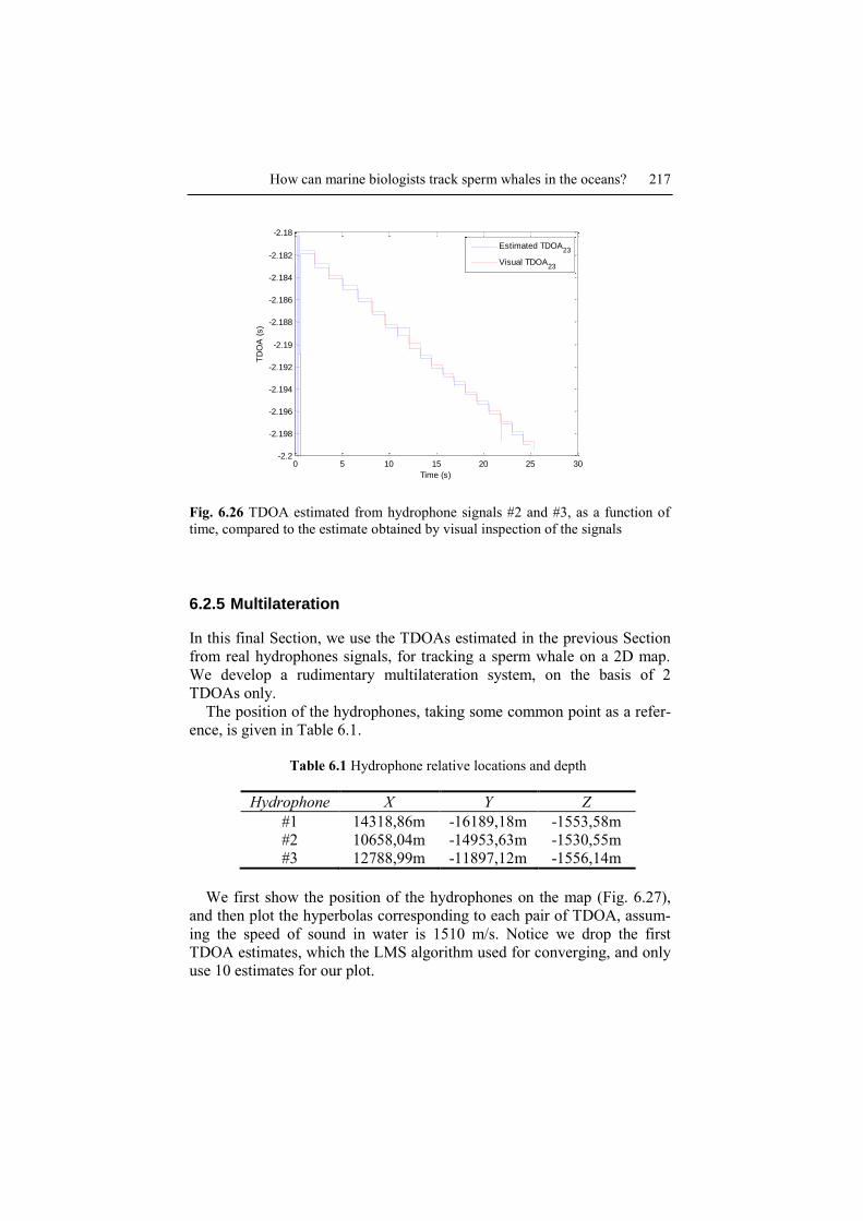
We repeat the operation for hydrophone signals #2 and #3 (Fig. 6.26).


0 5 10 15 20 25 30-2.2

-2.198

-2.196

-2.194

-2.192

-2.19

-2.188

-2.186

-2.184

-2.182

-2.18

Time (s)

TD

OA

(s)

Estimated TDOA23

Visual TDOA23

Fig. 6.26 TDOA estimated from hydrophone signals #2 and #3, as a function of

time, compared to the estimate obtained by visual inspection of the signals

6.2.5 Multilateration

In this final Section, we use the TDOAs estimated in the previous Section

from real hydrophones signals, for tracking a sperm whale on a 2D map.

We develop a rudimentary multilateration system, on the basis of 2

TDOAs only.

The position of the hydrophones, taking some common point as a refer-

ence, is given in Table 6.1.

Table 6.1 Hydrophone relative locations and depth

Hydrophone X Y Z

#1 14318,86m -16189,18m -1553,58m

#2 10658,04m -14953,63m -1530,55m

#3 12788,99m -11897,12m -1556,14m

We first show the position of the hydrophones on the map (Fig. 6.27),

and then plot the hyperbolas corresponding to each pair of TDOA, assum-

ing the speed of sound in water is 1510 m/s. Notice we drop the first

TDOA estimates, which the LMS algorithm used for converging, and only

use 10 estimates for our plot.


TDOA_12=TDOA_12(6000:length(TDOA_12)/10:end); TDOA_23=TDOA_23(6000:length(TDOA_23)/10:end); sound_speed=1510; % m/s for i=1:length(TDOA_12) PlotHyp(hydrophone_pos(1,1), hydrophone_pos(1,2), ... hydrophone_pos(2,1), hydrophone_pos(2,2), ... -TDOA_12(i)*sound_speed/2,'b'); PlotHyp(hydrophone_pos(2,1), hydrophone_pos(2,2), ... hydrophone_pos(3,1), hydrophone_pos(3,2), ... -TDOA_23(i)*sound_speed/2,'r'); end;

1.05 1.1 1.15 1.2 1.25 1.3 1.35 1.4 1.45

x 104

-1.65

-1.6

-1.55

-1.5

-1.45

-1.4

-1.35

-1.3

-1.25

-1.2

-1.15x 10

4

1

2

3

x (m)

y (

m)

1.0836 1.0838 1.084 1.0842 1.0844 1.0846

x 104

-1.4855

-1.485

-1.4845

-1.484

-1.4835

-1.483

-1.4825

-1.482

x 104

x (m)

y (

m)

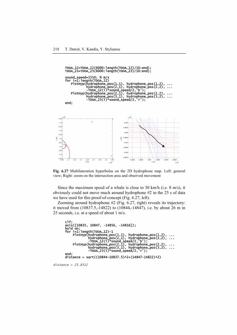
Fig. 6.27 Multilateration hyperbolas on the 2D hydrophone map. Left: general

view; Right: zoom on the intersection area and observed movement

Since the maximum speed of a whale is close to 30 km/h (i.e. 8 m/s), it

obviously could not move much around hydrophone #2 in the 25 s of data

we have used for this proof-of-concept (Fig. 6.27, left).

Zooming around hydrophone #2 (Fig. 6.27, right) reveals its trajectory:

it moved from (10837.5,-14822) to (10844,-14847), i.e. by about 26 m in

25 seconds, i.e. at a speed of about 1 m/s.

clf; axis([10835, 10847, -14856, -14816]); hold on; for i=1:length(TDOA_12)-1 PlotHyp(hydrophone_pos(1,1), hydrophone_pos(1,2), ... hydrophone_pos(2,1), hydrophone_pos(2,2), ... -TDOA_12(i)*sound_speed/2,'b'); PlotHyp(hydrophone_pos(2,1), hydrophone_pos(2,2), ... hydrophone_pos(3,1), hydrophone_pos(3,2), ... -TDOA_23(i)*sound_speed/2,'r'); end; distance = sqrt((10844-10837.5)^2+(14847-14822)^2)

distance = 25.8312


6.3 Going further

Readers interested in methods for estimating the position of a source from

multiple TDOA estimations should report to (Huang et al. 2008).

MATLAB code for localization, including more elaborate multilatera-

tion algorithms, is available from the Beam Reach Marine Science and

Sustainability School (Beam Reach 2007).

ISHMAEL (Integrated System for Holistic Multi-channel Acoustic Ex-

ploration and Localization) is free software for acoustic analysis, including

localization , made freely available by Prof. Dave Mellinger at Oregon

State University(Mellinger 2008). The same group also provides Moby-

Sound, a public a database for research in automatic recognition of marine

animal calls (Mellinger 2007).

MATLAB-based UWB positioning software can also be found in Senad

Canovic‟s Master thesis, from Norwegian University of Science and Tech-

nology (Canovic 2007).

6.4 Conclusion

In this Chapter, we have provided signal processing solutions for cleaning

impulsive signals mixed in noise and low-frequency interferences, and for

automatically estimating TDOAs based on either generalized cross-

correlation or adaptive filtering.

Although we have examined these techniques in the specific context of

whale spotting, they can easily be generalized to many positioning prob-

lems, such as the localization of speakers in a room, that of GSM mobile

phones, of Global Positioning System (GPS) receivers, or to that of air-

crafts or vehicles using either sonar or radar.

Last but not least, this Chapter also highlights one of the many “natural”

abilities of human beings: that of using both ears to locate sound sources.

6.5 References

Adam O (2005) Website of the 2nd International Workshop on Detection and Lo-

calization of Marine Mammals using Passive Acoustics [online] Available:

http://www.circe-asso.org/workshop/ [26/4/2008]

Adam O, Motsch JF, Desharnais F, DiMarzio N, Gillespie D, Gisiner RC (2006)

Overview of the 2005 workshop on detection and localization of marine

mammals using passive acoustics, Applied Acoustics 67:1061–1070

http://en.wikipedia.org/wiki/Global_System_for_Mobile_Communications

http://en.wikipedia.org/wiki/Mobile_phone




Beam Reach (2007) Acoustic Localization [online] Available:

http://beamreach.org/soft/AcousticLocation/AcousticLocation-041001/

[23/6/2008]

Benesty J (2000) Adaptive eigenvalue decomposition algorithm for passive acous-

tic source localization. J. Acoust. Soc. Am. 107 (1): 384–391

Canovic S (2007) Application of UWB Technology for Positioning , a Feasibility

Sudy. Master thesis, Norwegian University of Science and Technology [on-

line] Available:

http://www.diva-portal.org/ntnu/undergraduate/abstract.xsql?dbid=2091

[23/06/08]

Huang Y, Benesty J, Chen J (2007) Time delay estimation and source localization.

In Springer Handbook of Speech Processing, Benesty J, Sondhi MM, Huang

Y (eds), Springer:Berin, 51:1043–1063

Drouot V (2003) Ecology of sperm whale (Physeter macrocephalus) in the Medi-

terranean Sea. Ph.D. Thesis, Univ. of Whales, Bangor, UK

Fang J, Atlas LE (1995) Quadratic detectors for energy estimation. IEEE Transac-

tions on Signal Processing 43–11: 2582–2594

Huang Y, Benesty J, Chen J (2008) Time delay estimation and source localization.

In: Springer Handbook of Speech Processing, Benesty J, Sondhi MM, Huang

Y (Eds.), Springer: Berlin. 1043–1063.

Kaiser JF (1990) On a simple algorithm to calculate the „„Energy‟‟ of a signal. In:

Proc. IEEE ICASSP, 381–384, Albuquerque, NM, USA

Kandia V, Stylianou Y (2005) Detection of creak clicks of sperm whales in low

SNR conditions. In CD Proc. IEEE Oceans, Brest, France

Kandia V, Stylianou Y (2006) Detection of sperm whale clicks based on the Tea-

ger–Kaiser energy operator, Applied Acoustics 67:1144–1163

Kandia V, Stylianou Y (2006) Accurate TDOA (Time Difference of Arrival) using

the Teager – Kaiser Energy Operator. In CD Proceedings of the 20th Annual

Conference of the European Cetacean Society, Gdynia, Poland

Knapp CH and Carter GC (1976) The generalized correlation method for estima-

tion of time delay. In: IEEE Transactions on Acoustic, Speech and Signal

Processing 24, 320–327

ICES (International Council for the Exploration of the Sea - Advisory Committee

on Ecosystems, ICES CM 2005/ACE:01) (2005) Report of the Ad-hoc Group

on the Impact of Sonar on Cetaceans and Fish (AGISC).

Madsen PT (2002) Sperm whale sound production – in the acoustic realm of the

biggest nose on record, In Madsen P.T., PhD. Dissertation, Sperm whale

sound production., Dep. of Zoophysiology, University of Aarhus, Denmark

Mellinger D (2007) MobySound [online] Available:

http://hmsc.oregonstate.edu/projects/MobySound/ [23/6/2008]

Mellinger D (2008) Ishmael Integrated System for Holistic Multi-channel Acous-

tic Exploration and Localization [online] Available:

http://www.pmel.noaa.gov/vents/acoustics/whales/ishmael [23/6/2008]

Morrissey RP, Ward J, DiMarzio N, Jarvis S, Moretti DJ (2006) Passive acoustic

detection and localization of sperm whales (Physeter macrocephalus) in the

tongue of the ocean. Applied Acoustics 67:1091–1105

http://www.amazon.com/exec/obidos/search-handle-url/002-9062137-4968034?%5Fencoding=UTF8&search-type=ss&index=books&field-author=Jacob%20Benesty

http://www.amazon.com/exec/obidos/search-handle-url/002-9062137-4968034?%5Fencoding=UTF8&search-type=ss&index=books&field-author=M.%20Mohan%20Sondhi

http://www.amazon.com/exec/obidos/search-handle-url/002-9062137-4968034?%5Fencoding=UTF8&search-type=ss&index=books&field-author=Yiteng%20Huang

http://www.ices.dk/iceswork/wgdetailace.asp?wg=AGISC

http://www.ices.dk/iceswork/wgdetailace.asp?wg=AGISC


Møhl B, Wahlberg M, Madsen PT, Heerfordt A, Lund A (2000) Sperm whale

clicks: Directionality and source level revisited, J. Acoust. Soc. Am. 107 (1):

638–648.

Sicuranza G (1992) Quadratic filters for signal processing. In: Proceedings of the

IEEE, 80(8):1263–1285

Widrow B, Stearns SD (1985) Adaptive Signal Processing. Prentice-Hall,Inc.,

Upper Saddle River, NJ

Zimmer WMX, Madsen PT, Teloni V, Johnson MP, Tyack PL (2005) Off-axis ef-

fects on the multi-pulse structure of sperm whale usual clicks with implica-

tions for the sound production. J. Acoust. Soc. Am. 118: 3337–3345

how can marine biologists track sperm whales in...

Documents