How are photospheric flows related to solar flares?

Brian T. Welsch1, Yan Li1,Peter W. Schuck2, & George H. Fisher1

1SSL, UC-Berkeley2NASA-GSFC

See also ApJ v. 705 p. 821

Outline• We don’t understand processes that produce flares and coronal mass ejections (CMEs),

but would like to.

• Electric currents in the coronal magnetic field Bc power flares and CMEs, but measurements of (vector) Bc are rare and subject to large uncertainties.

• The instantaneous state of the photospheric field BP provides limited information about the coronal field Bc.

• Properties of photospheric field evolution can reveal additional information about the coronal field.

• We used tracking methods (and other techniques) to quantitatively analyze photospheric magnetic evolution in a few dozen active regions (ARs).

• We found a “proxy Poynting flux” to be statistically related to flare activity. This association merits additional study.

Flares are transient enhancements of the Sun’s radiative output over a wide wavelength range, from radio to X-rays.

This movie shows flare emission in Ca II ob-served by the Solar Optical Telescope (SOT) aboard the Hinode satellite. (Image credit: SOT Team/NASA/JAXA)

Flares produce bursts of emission in spaceborne X-ray monitors.

Note “two ribbon” structure

Flares arise from the release of energy stored in electric currents in the coronal magnetic field.

Movie credit: EIT team McKenzie 2002

the “standard model”an EUV movie of ~1MK thermal emission

Active region (AR) magnetic fields produce flares and CMEs.

Magnetograms are maps of the photo-spheric magnetic field.

White/black show areas of positive/negative magnetic flux.

Magnetograms are derived from spectropolarimetric measurements.

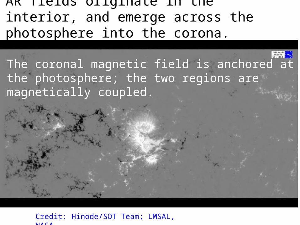
AR fields originate in the interior, and emerge across the photosphere into the corona.

The coronal magnetic field is anchored at the photosphere; the two regions are magnetically coupled.

Credit: Hinode/SOT Team; LMSAL, NASA

What physical processes produce coronal electric currents? Two options are:• Currents could form in the interior, then emerge into

the corona.– Current-carrying magnetic fields have been observed to

emerge (e.g., Leka et al. 1996, Okamoto et al. 2008)

• Photospheric evolution could induce currents in already-emerged coronal magnetic fields.

– From simple scalings, McClymont & Fisher (1989) argued induced currents would be too weak to power large flares

– Detailed studies by Longcope et al. (2007) and Kazachenko et al. (2009) suggest strong enough currents can be induced

General picture: slow buildup, sudden release.

Measuring the coronal vector field BC is difficult, but the photospheric BP and BLOS are routinely measured.

Coronal field measurements are scarce, and subject to large uncertainties (e.g., Lin, Kuhn, & Coulter 2004).

While photospheric magnetograms are relatively common, only BLOS, the line-of-sight (LOS) component of the vector BP has been routinely measured.(This should change soon, with NSO’s SOLIS and NASA’s HMI.)

How are photospheric fields related to flare activity?

Schrijver (2007) associated large flares with the amount of magnetic flux near strong-field polarity inversion lines (PILs).

R is the total unsigned flux near strong-field PILs

AR 10720, and its masked PILs at right

Discriminant analysis can test the capability of a magnetic parameter to predict flares.

1) For a time window t, estimate distribution functions for the parameter in the flaring (green) and nonflaring (black) populations in a “training dataset.”

2) Given an observed value, predict a flare within the next t if:

Pflare > Pnon-flare

(vertical blue line) From Barnes and Leka 2008

Barnes & Leka (2008) tested R against , and found them to be equally bad flare predictors!

Barnes & Leka (2008) tested R against , and found them to be equally bad flare predictors!

• Large flares are rare, so it’s a good bet that no flare will occur in a forecast window of a day or less. “Success rates” > 90% are possible by “just saying no”

Barnes & Leka (2008) tested R against , and found them to be equally bad flare predictors!

• Large flares are rare, so it’s a good bet that no flare will occur in a forecast window of a day or less. “Success rates” > 90% are possible by “just saying no”

• “Skill scores” are normalized to expected rate– 1 = perfect forecast; 0 merely matches expectation – Heidke = “just say no”; “Climate” = historical rate

It turns out that a snapshot of the photospheric vector field BP isn’t very useful for predicting flares.

• Leka & Barnes (2007) studied 1200 vector magnetograms, and considered many quantitative measures of AR field structure.

• They summarize nicely: “[W]e conclude that the state of the photospheric magnetic field at any given time has limited bearing on whether that region will be flare productive.”

Can we learn anything about flares from the evolution of BP?

When not flaring, coronal magnetic evolution should be nearly ideal photospheric connectivity is preserved.

As BP evolves, changes in BC are induced.

Further, following AR fields in time can provide information about their history and development.

30

Assuming BP evolves ideally (e.g., Parker 1984), then photospheric flow and magnetic fields are coupled.

• The magnetic induction equation’s z-component relates the flux transport velocity u to dBz/dt (Demoulin & Berger 2003).

Bz/t = [ x (v x B) ]n = - (u Bn)

• Many “optical flow” methods to estimate u have been developed, e.g., LCT (November & Simon 1988), FLCT (Welsch et al. 2004), DAVE (Schuck 2006).

The apparent motion of magnetic flux in magnetograms is the flux transport velocity, uf.

uf is not equivalent to v; rather, uf vhor - (vn/Bn)Bhor

• uf is the apparent velocity (2 components)

• v is the actual plasma velocity (3 comps)

(NB: non-ideal effects can also cause flux transport!)

Démoulin & Berger (2003): In addition to horizontal flows, vertical velocities can lead to uf 0. In this figure, vhor= 0, but vn 0, so uf 0.

Aside: Flows v|| along B do not affect Bn/t, but “contaminate” Doppler measurements.

vLOSvLOS

vLOS

Photospheric electric fields can affect flare-related magnetic structure in the corona.

• If magnetic evolution is ideal, then E = -(v x B)/c, and the Poynting flux of magnetic energy across the photosphere depends upon v:

∂tU = c ∫ dA (E x B) ∙ n / 4π = ∫ dA (B x (v x B)) ∙ n / 4π

• BC BP coupling means the surface v provides an essential boundary condition for data-driven MHD simulations of BC. (Abbett et al., in progress).

• Studying v could also improve evolutionary models of BP , e.g., flux transport models.

35

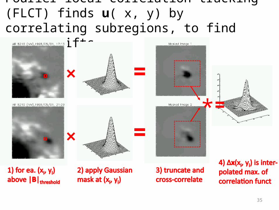
Fourier local correlation tracking (FLCT) finds u( x, y) by correlating subregions, to find local shifts.

*

=

==

We studied flows {u} from MDI magnetograms and flares from GOES for a few dozen active region (ARs).

• NAR = 46 ARs were selected.– ARs were selected for easy tracking – usu. not

complex, mostly bipolar -- NOT a random sample!

• > 2500 MDI full-disk, 96-minute cadence magnetograms from 1996-1998 were tracked, using both FLCT and DAVE separately.

• GOES catalog was used to determine source ARs for flares at and above C1.0 level.

Magnetogram Data Handling

• Pixels > 45o from disk center were not tracked.

• To estimate the radial field, cosine corrections were used, BR = BLOS/cos(Θ)

• Mercator projections were used to conformally map the irregularly gridded BR(θ,φ) to a regularly gridded BR(x,y).

• Corrections for scale distortion were applied.

FLCT and DAVE flow estimates are correlated, but differ significantly.

When weighted by the estimated radial field |BR|, the FLCT-DAVE correlations of flow components were > 0.7.

For both FLCT and DAVE flows, speeds {u} were not strongly correlated with BR --- rank-order correlations were 0.07 and -0.02, respectively.

The highest speeds were found in weak-field pixels, but a range of speeds were found at each BR.

To baseline the importance of field evolution, we analyzed properties of BR, including:

- 4 statistical moments of average unsigned field |BR| (mean, variance, skew, kurtosis), denoted M(|BR|)

- 4 moments M( BR2 )

- total unsigned flux, = Σ |BR| da2

- total unsigned flux near strong-field PILs, R (Schrijver 2007)

- sum of field squared, Σ BR2

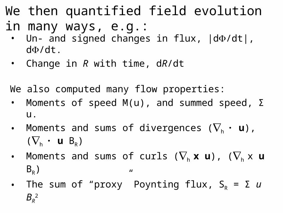
We then quantified field evolution in many ways, e.g.:

• Un- and signed changes in flux, |d/dt|, d/dt.• Change in R with time, dR/dt

We also computed many flow properties:• Moments of speed M(u), and summed speed, Σ u.• Moments and sums of divergences (h · u), (h · u BR)

• Moments and sums of curls (h x u), (h x u BR)

• The sum of “proxy” Poynting flux, SR = Σ u BR2

To find a typical flow timescale, we autocorrelated ux, uy, and BR, for both FLCT and DAVE flows.

BLACK shows autocorrelation for BR; thick is current-to-previous, thin is current-to-initial.

BLUE shows autocorrelation for ux; thick is current-to-previous, thin is current-to-initial.

RED shows autocorrelation for uy; thick is current-to-previous, thin is current-to-initial.

Parametrization of Flare Productivity

• We binned flares in five time intervals, τ: – time to cross the region within 45o of disk center (few days);– 6C/24C: the 6 & 24 hr windows centered each flow estimate;– 6N/24N: the “next” 6 & 24 hr windows after 6C/24C

(6N is 3-9 hours in the future; 24N is 12-36 hours in the future)

• Following Abramenko (2005), we computed an average GOES flare flux [μW/m2/day] for each window:

F = (100 S(X) + 10 S(M) + 1.0 S(C) )/ τ ;exponents are summed in-class GOES significands

• Our sample: 154 C-flares, 15 M-flares, and 2 X-flares

Correlation analysis showed several variables associated with flare flux F. This plot is for disk-passage averaged properties.

Field and flow properties are ranked by distance from (0,0), the point of complete lack of correlation.

Only the highest-ranked properties tested are shown.

The more FLCT and DAVE correlations agree, the closer they lie to the diagonal line (not a fit).

Many of the variables correlated with average flare SXR flux were correlated with each other.

Such correlations had already been found by many authors.

Leka & Barnes (2003a,b) used discriminant analysis (DA) to find variables most strongly associated with flaring.

Given two input variables, DA finds an optimal dividing line between the flaringflaring and quiet populations.

The angle of the dividing line can indicate which variable discriminates most strongly.

Blue circles are means of the flaringflaring and non-flaring populations.

(With N input variables, DA finds an N-1 dim-ensional surface to partition the N-dimen-sional space.)

Standardized “proxy Poynting flux,” SR = Σ u BR2

Sta

ndar

dize

d S

tron

g-fie

ld P

IL F

lux R

We used discriminant analysis to pair field/ flow properties

“head to head” to identify the strongest flare associations.

For all time windows, regardless of whether FLCT or DAVE flows were used, DA consistently ranked Σ u BR

2 among the two most powerful discriminators.

Physically, why is the proxy Poynting flux, SR = Σ uBR2,

associated with flaring? Further study is needed.

u BR2 corresponds to the part of the horizontal

Poynting flux, from Eh x Br

– The vertical Poynting flux, due to Eh x Bh, is probably most relevant to flaring.

– Another component of the horizontal Poynting flux, from Er x Bh, is neglected in our analysis.

Are horizontal & vertical Poynting fluxes similar in magnitude? Why would this be?

Do flows from flux emergence or rotating sunspots also produce large values of SR?

Distinct regions contribute to the sums for R and SR , implying different underlying physical processes.

White regions show strong contributions to R and SR in AR 8100; white/black contours show +/- BR at 100G, 500G.

ConclusionsWe found Σ u BR

2 and R to be strongly associated with average flare soft X-ray flux and flare occurrence.

Σ u BR2 seems to be a robust flare predictor:

- speed u was only weakly correlated with BR; - Σ BR

2 was independently tested;- using u from either DAVE or FLCT gave similar results.

It appears that ARs that are both relatively large and rapidly evolving are more flare-prone.

This study suffers from low statistics; further study is needed. (A proposal to extend this work has been submitted!)