how applicable is the inflation- targeting framework for ... · the inflation-targeting framework...
TRANSCRIPT

123
S H E E T A L K . C H A N DUniversity of Oslo
K A N H A I Y A S I N G HNCAER
How Applicable Is the Inflation-Targeting Framework for India?
Akey component in stabilizing an economy is keeping the rateof inflation within acceptable bounds and doing so in a manner
that does not detract from other goals. This is a difficult exercise, and therehave been many failures both in the advanced economies and especially inemerging economies. The record of inflation control in India, while notunsatisfactory, could have been better. Inflation in the first half of 2005–06is around 5 percent, which is relatively high in the current global environmentof mild inflation and, contingent on the handling of the ongoing oil priceincreases, could easily ratchet upward. The issue of inflation control inIndia is therefore important. In recent years, several countries have adoptedthe inflation-targeting framework (ITF) approach, which is now beingstrongly recommended to others as a best-practice approach for keepinginflation under control. Although it is still too early to tell whether or notthe approach has been decisive in reducing inflation rates—its introductioncoincided with a period of exceptional weakness in commodity prices fol-lowing the break up of the Soviet Union—a strong theoretical case hasbeen made for it.1 Detailed operational guidelines and procedures have alsobeen developed for its application.2
Essentially the ITF approach consists of setting an inflation target, align-ing monetary policy to ensure its attainment, and doing so in a manner thatis both transparent and accountable. The target is set publicly and consider-able information is made available to the public regarding the modalities
The authors are indebted for helpful comments from participants and especially BarryBosworth, Ken Kletzer, and Rajnish Mehra, who are not, however, responsible for anyremaining errors and omissions.
1. See especially Svensson (1997).2. See, for example, various reports of the Bank of England. Bernanke and others (2001)
provide some useful historical details.

124 IND IA POL ICY FORUM, 2006
for achieving it in an attempt to establish credibility and to manage inflationexpectations. A major advantage claimed for the ITF is that it enables focus-ing on the inflation target in a nonmechanical, flexible way that can takeaccount of various contingencies and possible trade-offs with other object-ives such as the level of economic activity.
For a country to be able to apply the ITF successfully, it must have strongfiscal and financial institutions and a balanced exposure to foreign exchangerisks. Questions have therefore been raised about whether many emergingeconomies qualify for the ITF. Some of them, including India, have largefiscal deficits, and others such as China have weak banks and financialinstitutions. Moreover, most of them appear to exhibit a “fear of floating”and intervene to stabilize the exchange rate, thereby compromising the prac-tice of inflation targeting. However, some have argued that, provided theauthorities in these economies are sufficiently motivated to want the benefitsof inflation targeting, they should not delay but use the introduction of theITF as an incentive device to promote needed reforms in economic structure.3
It is presumably in this spirit that the International Monetary Fund (IMF)and other agencies have been encouraging emerging economies to adoptthe ITF.4
In making these recommendations, it is taken for granted that the ITF isan appropriate institution for emerging economies such as India. But thisassumption may be questionable. The issue is not that of denying the import-ance of a low inflation rate; indeed, for India it has been amply demonstratedthat the lower the inflation rate the more favorable the growth outcome.5
The issue, which this paper focuses on, is whether lower inflation is bestbrought about through the adoption of ITF. At the heart of the ITF is aspecific view of the inflation-generating process determined largely bydemand, a conviction that the most efficient way of dealing with it is throughan interest rate rule, and the belief that the public’s inflation expectationscan be managed. From this follows the prescription that the central bank,as the custodian of interest rate policy, should play a dedicated and dominantrole in promoting the inflation objective.
But what if the inflation-generating process differs from that commonlyassumed to hold for the advanced economies? For example, supply shocksand price management could feature more prominently than demand effects,while the latter could be influenced by a different array of instruments.
3. See Mishkin (2004), among others.4. See, for example, IMF (2005).5. Singh and Kalirajan (2003) provide a demonstration.

Sheetal K. Chand and Kanshaiya Singh 125
Expectations could also be more difficult to manage, especially if the econ-omy is large, diverse, and segmented as is India’s. But aside from theseconsiderations, emerging economies may have good reasons for not wantingto free up fully the process of interest and exchange rate determination bythe market. They may fear being exposed to persistent deviations in the ex-change and interest rates from equilibrium levels and also to greater volatilityin them, since they lack the hedging capabilities and facilities present inthe advanced economies. All this implies that these emerging economiesmay find it more prudent and welfare enhancing f to pursue a strategy otherthan the standard ITF for controlling inflation, at least until they reproduceconditions favorable for an ITF.6 They will then have to seek nominal anchorselsewhere.
In analyzing these issues, this paper first presents the rationale for theITF and examines a standard theoretical formulation based on Svensson’swork. The central proposition of this formulation is tested on Indian dataand found inadmissible. Rather than accept the implication of that specifi-cation that demand does not affect the inflation rate, an alternative structurefor determining inflation is then developed. This shows how demand mayplay a role in influencing the inflation rate as part of a broader scheme, andthe choices of instruments for dealing with inflation. Testing on Indian datais more favorable to the alternative specifications developed. In light of thefindings, the paper then examines how best to ensure an adequate inflationperformance and the implied institutional allocation of responsibilities.A sharp distinction is drawn between “flow” responsibilities concerningoperations in the goods market for which a combination of fiscal, credit,and supply-price management policies may be appropriate and “stock”responsibilities involving balance-sheet operations to influence asset valu-ations in desirable directions. As will be seen, this distinction determines aspecific allocation of responsibilities in the Indian context between the gov-ernment and the central bank.
A Rationale and Test of ITF Using Indian Data
Controlling inflation has traditionally been viewed as a matter of anchoringthe money supply. The issue arises specifically with fiduciary money, since
6. However, concerns over interest rate and exchange rate misalignments and volatilities,including especially their divergent asset market and goods market effects, could limit interestin the ITF.

126 IND IA POL ICY FORUM, 2006
its amount can be increased at virtually no cost. This section briefly reviewsthe evolution of views as to what constitutes a good anchor, culminating inthe inflation forecast targeting rule, which is then tested on Indian data.
Why an ITF?
In a textbook closed economy, controlling the money stock is a sufficientanchor, while in an open economy, the traditional approach to anchoringthe money supply is to peg the exchange rate. Observing the peg enforces theneeded discipline on the central bank as it cannot expand the money supplyexcessively without suffering a loss of international reserves, which willthreaten the peg. However, the increasing trend to capital market liberal-ization rendered the exchange rate peg more vulnerable to large swings incapital flows. Following a number of spectacular failures in both developedand emerging economies to maintain the peg in the face of speculativepressures, pegged exchange rates were largely abandoned in favor of floatingexchange rates.
Since a floating exchange rate regime confers considerable independenceon monetary policy, the issue of its anchor had to be resolved; generally ananchor was achieved through adoption of money supply targets. Financialinnovations, however, have made money demand growth unstable and unpre-dictable, and thus the experience with monetary targeting has not been satis-factory. Pursuit of a given rate of growth in a selected monetary aggregatecould result in unacceptable inflation rates.
As monetary targeting is abandoned, emphasis is increasingly beingplaced directly on the inflation rate. If the principal consequence of undis-ciplined monetary policy is the generation of unacceptable inflation rates,an alternative to attempting to control an elusive monetary aggregate wouldbe to target the inflation rate and to seek instruments that would realize it.In pursuit of the inflation target, the central bank must be free to use itsinterest rate instrument, since this is the only alternative to money supplytargeting available to it. But this in turn implies that the central bank cannotbe diverted by any simultaneous need to influence the exchange rate. Rulingout the exchange rate, interest rates, and monetary aggregate as potentialanchors implies that the anchoring role is instead performed by the inflationtarget.
Beginning with New Zealand, an increasing number of countries haveadopted inflation targeting. There is little doubt that the ITF countries haveimproved their inflation record after adopting this framework (table 1).The actual mechanism that reduced inflation is an open question, however.

Sheetal K. Chand and Kanshaiya Singh 127T
AB
LE
1.
Coef
ficie
nt o
f Var
iatio
n of
Exc
hang
e Ra
te in
Uni
ted
Stat
es, J
apan
, Ind
ia a
nd S
elec
ted
Infla
tion-
Targ
etin
g Co
untr
ies
Exch
ange
rate
var
iatio
nCP
I Inf
latio
n (m
ean)
Durin
g 3
year
sDu
ring
first
3Du
ring
full
perio
dDu
ring
3 ye
ars
Durin
g fir
st 3
Durin
g fu
llIT
F da
tebe
fore
ITF
year
s af
ter I
TFaf
ter I
TFbe
fore
ITF
year
s af
ter I
TFpe
riod
afte
r ITF
Braz
ilQ2
-199
920
.86
17.0
824
.28
6.83
6.78
8.34
Chile
Q1-1
991
11.1
77.
8123
.57
19.4
517
.69
7.25
Sout
h Af
rica
Q1-2
000
13.1
520
.25
22.7
06.
607.
045.
51Is
rael
Q1-1
992
9.07
8.35
19.2
318
.64
11.9
02.
03Pe
ruQ1
-199
440
.44
6.95
16.6
772
1.51
15.2
16.
49Cz
ech
Repu
blic
Q1-1
999
10.0
04.
7916
.29
8.84
3.60
2.58
Icel
and
Q1-2
001
8.77
14.1
816
.18
3.41
4.36
4.12
New
Zea
land
Q1-1
990
5.70
0.07
15.8
99.
172.
572.
28Hu
ngar
yQ1
-200
112
.47
13.3
315
.41
11.2
76.
4111
.32
Aust
ralia
Q4-1
994
6.06
6.59
15.2
11.
612.
322.
68Sw
eden
Q1-1
995
15.2
07.
3514
.76
3.46
0.98
1.16
Switz
erla
ndQ1
-200
05.
408.
6013
.78
0.54
1.06
0.92
Norw
ayQ1
-200
17.
5212
.59
13.6
72.
641.
981.
82Co
lom
bia
Q3-1
999
21.9
010
.57
13.3
917
.42
8.14
7.49
Mex
ico
Q1-1
999
10.8
62.
668.
1523
.56
10.3
87.
80Po
land
Q4-1
998
12.6
75.
997.
7316
.11
7.77
5.02
Cana
daQ1
-199
25.
785.
637.
723.
141.
211.
83Ko
rea
Q1-1
998
30.2
68.
287.
574.
953.
093.
51Un
ited
King
dom
Q1 1
993
8.25
2.78
6.74
6.02
2.51
2.52
Thai
land
Q2-2
000
4.70
3.72
4.73
3.62
1.39
1.72
Unite
d St
ates
aQ1
-199
52.
495.
046.
142.
872.
502.
46In
diaa
Q1-1
995
9.37
7.71
12.5
69.
808.
876.
41Ja
pana
Q1-1
995
10.4
813
.26
10.5
01.
360.
70–0
.05
Sour
ce: B
asic
dat
a co
me
from
IMF
(200
5).
Note
: All
varia
tions
are
repo
rted
in U
S$, e
xcep
t for
var
iatio
ns fo
r the
Uni
ted
Stat
es, w
hich
are
repo
rted
in s
peci
al d
raw
ing
right
s. D
ata
excl
ude
the
cris
is p
erio
d fo
rBr
azil,
and
199
7–20
00 fo
r Tha
iland
. Chi
le h
ad a
cra
wlin
g pe
g be
fore
199
1. M
exic
o ha
s an
oil
fund
.a.
Cou
ntrie
s do
not
hav
e an
infla
tion-
targ
etin
g fr
amew
ork.

128 IND IA POL ICY FORUM, 2006
Was it the intention to target inflation, was it the inflation-targeting frame-work, or were some other exogenous factors responsible?
The rigorous implementation of the ITF would imply increased volatilityin variables such as the exchange rate. A close look at the quarterly variationin exchange rates during the three years before and the three years after im-plementation of the ITF indicates a mixed outcome (see table 1 and figure 1,where variation in the U.S. dollar is reported with respect to special drawingrights, while variation in the currencies of other countries is reported withrespect to the U.S. dollar). For most of the ITF countries (with the exceptionof Hungary, Iceland, Norway, South Africa, and Switzerland), the volatilityin nominal exchange rate, measured as a coefficient of variation with respectto the U.S. dollar, was reduced during the first three years of implementation.
When a longer period after implementation of the ITF is considered,however, the coefficient of variation increases considerably beyond the initialthree-year period in almost all cases. One explanation is that the countrieshave, contrary to the ITF requirements, engaged in a “dirty” peg of theirdomestic currency to the dollar as a way to reduce inflation, since the UnitedStates is a low-inflation, low-interest-rate country. Most of the ITF countriesappear to have adopted this strategy in the initial period following the adop-tion of the ITF. Having achieved reasonable stability, monetary policy isthen better aligned with ITF requirements; that situation is reflected in amore volatile exchange rate during the later periods. Such volatility couldalso be partially attributable to an increase in the volatility of the U.S. dollar.While it is difficult to fully disentangle the contributions of these alternativeexplanations, the data give some support to the implication that the ITFleads to volatile asset markets, indicating that at least some of the countrieswere more rigorous in their application of the ITF.
In general, for countries to be able to abandon traditional anchors infavor of inflation targeting, their economies must have the capacity to toleratewide swings in nominal interest rates and in the nominal exchange rate. Onthe stock side, these swings will exert valuation effects. They may contributeto mismatches between different categories of assets and liabilities onbalance sheets. This could generate various problems both in the financingand production spheres as became readily apparent during the Asian crisisof the late 1990s. Firms that borrow short in one currency and invest longin another may find their net worth wiped out. Declines in asset valuesaffect both the ability of firms to borrow from banks and the desire ofindividuals to spend. Deterioration in investment and consumption activitieswill then act as a drag on output growth.

Sheetal K. Chand and Kanshaiya Singh 129F
IGU
RE
1.
Coef
ficie
nt o
f Var
iatio
n of
Exc
hang
e Ra
te in
Uni
ted
Stat
es, J
apan
, Ind
ia a
nd S
elec
ted
Infla
tion-
Targ
etin
g Co
untr
ies
Sour
ce: B
asic
dat
a co
me
from
IMF
(200
5).
Note
: All
varia
tions
are
repo
rted
in U
S$, e
xcep
t for
var
iatio
ns fo
r the
Uni
ted
Stat
es, w
hich
are
repo
rted
in s
peci
al d
raw
ing
right
s. D
ata
excl
ude
the
cris
is p
erio
dfo
r Bra
zil, a
nd 1
997–
2000
for T
haila
nd. C
hile
had
a c
raw
ling
peg
befo
re 1
991.
Mex
ico
has
an o
il fu
nd.
a. C
ount
ries
do n
ot h
ave
an in
flatio
n-ta
rget
ing
fram
ewor
k.

130 IND IA POL ICY FORUM, 2006
In a world of sticky prices, nominal swings in interest and exchangerates also imply corresponding fluctuations in their real counterparts. Thesefluctuations affect relative prices and have additional implications for flowbehavior. A change in real interest rates affects the terms of trade betweenthe present and the future, thereby influencing investment and savingsbehavior. Real exchange rate adjustments modify the relative price ratiosbetween tradable and nontradable goods, and between home and foreigngoods, that affect profitability in the respective sectors. These changes alsocontribute to changing production and investment patterns. Of particularconcern is the phenomenon of exchange rate overshooting. For example,when interest rates are tightened, the exchange rate overappreciates so asto induce an expectation of subsequent depreciation in order to balancefinancial markets. But this overappreciation could have serious adverseconsequences for the country’s international trade.
Volatility in real interest rates and exchange rates can thus be disruptive.Not surprisingly, in emerging market economies widely believe that theirdevelopmental needs are better served by stable real exchange interest rates,provided these are set at appropriate levels. Emerging economies such asChina, India, and Malaysia have had some success in pursuing a less volatileapproach with respect to these two key variables of interest and exchangerates.
Before deciding whether to adopt the ITF, an emerging economy shouldestablish how capable it is of withstanding the volatile stock-flow impli-cations that the ITF and its monetary actions entail. Most emerging econ-omies, including India despite its fairly developed financial sector, lack thehedging facilities and regulatory capabilities of advanced economies. How-ever, if the only instrument available for satisfactorily dealing with inflationis the nominal interest rate instrument, an emerging economy’s only alter-native may be adoption of the ITF. In that case, the volatility-related costsincurred on the financial stock side and the production sectors will have tobe tolerated. It is therefore important to test the suitability of the ITF’smode of applying monetary policy, and the availability of alternatives, beforemaking a decision.
Standard Theoretical Formulation
Svensson provides a clear exposition of the standard inflation-targetingapproach, which is used as the reference in the following discussion.7 He
7. Svensson (1997).

Sheetal K. Chand and Kanshaiya Singh 131
assumes a closed economy, and although in other papers he relaxes thatassumption, that is not essential for our purposes here.8 Since our concernis with the assumed transmission mechanism that links the monetary policyinstrument with the domestic rate of inflation, the analysis of the simplerclosed-economy case could be regarded as embedded in a more compre-hensive open-economy model. Simplifying even further, we assume, withSvensson, that the focus is on pure inflation targeting without any trade-offs with other objectives.
THE SVENSSON VERS ION . The model structure is as follows:
(1) 111 ++ ++= tttt x εαππ
(2) 1211 )( ++ +−−= ttttt ixx ηπββ
where πt = pt – pt–1 is the inflation rate in year t, pt is the log of the pricelevel, xt is the output gap defined as the log of actual to potential output, it
is the monetary policy instrument, and εt and ηt are i.i.d shocks in year tthat are not known in year t – 1. All coefficients are nonnegative; βt < 1.
The formulation of this model is based on stylized empirical factors asthey pertain to the advanced industrial economies. Equation 1 determinesinflation as a function of the preceding period’s inflation rate, output gap,and a stochastic shock. Equation 2 indicates that the output gap is a positivefunction of the previous period’s output gap and negatively affected by theex post real interest rate.
The model yields a reduced form solution for the inflation rate on takingnote of the assumed stylized lag structure and making the relevant substi-tutions. The important point is that there is a one-year lag between the out-put gap and the inflation rate, while the output gap responds to the previousyear’s real interest rate. In other words, the central bank, in setting thenominal interest rate, can only influence inflation two years down the road.
(3).),1(,1
where
)(
21312211
211113212
βαβαβα
εηαεππ
=+=+=
+++−+=
1
++++
aaa
iaxaa tttttt
8. Svensson (2003) reviews several variants of the basic model. See also Aghenor (2002)for an exposition. The main effect of opening the economy is to introduce another channelof influence through the exchange rate on the domestic rate of inflation. Since the exchangerate is floating, the effect would be in the same direction as the monetary action; for example,an appreciation accompanying a monetary tightening would accelerate the improvement inthe inflation rate.

132 IND IA POL ICY FORUM, 2006
The solution shows that the inflation rate that will prevail at time t + 2will be determined by the current profile of the specified key variables andthe relevant shocks that occur over the next two periods. Since those shockscannot be anticipated, the inflation rate expected at time t + 2 will be afunction only of current variable values and the interest rate instrumentsetting. An optimal inflation-targeting rule is obtained by minimizing thepresent expected value of an intertemporal loss function
(4) ∑∞
=
−
t
tt LEτ
ττ πδ )(
where δ ∈ (0,1) is the discount factor.The loss function for each period is specified as the squared deviation of
the inflation rate from the target level π*.
(5)2*)(
2
1)( πππ ττ −=L
The decision problem is to select a time path of nominal interest ratesthat will minimize the expected sum of discounted squared future deviationsof inflation from the target, subject to the constraint imposed by equation 3.This is a potentially complicated exercise in dynamic programming, butSvensson shows how the problem can be simplified by using the lag struc-ture. Since the central bank can only influence the inflation rate two periodsahead, the optimal interest rate in year t is found as the solution to a period-by-period problem.
(6) )(Min 22
+τπδ LEtit
The first-order condition for minimizing equation 6 with respect to it is
(7) 0*)()(
2322
2
=−−=∂
∂+
+ ππδπδ
ttt
tt Eai
LE
The condition is met if the expected rate of inflation two years henceequals the target rate. This is equivalent to equating the current two-yearinflation forecast (given by equation 3) to the target rate. On setting thisforecast equal to the target rate, the following optimal policy rule for thenominal interest rate is derived

Sheetal K. Chand and Kanshaiya Singh 133
(8)
2
12
211
21
1,
1
where
*)(
ββ
βα
πππ
+==
+−+=
bb
xbbi tttt
It is an inflation forecast targeting rule, which corresponds to the strictinflation-targeting version of the well-known Taylor rule.9 However, unlikethe Taylor rule, where the coefficients would either be arbitrary or somehowestimated from past data, Svensson’s derivation is based on the postulatedunderlying structure of the economy. His rule sets the interest rate by refer-ence to the deviation of the current inflation rate from the target rate. As hepoints out, this is not because current inflation is targeted, which it cannotbe since it is predetermined, but because current inflation is one of theinputs in predicting future inflation (see equation 3). The ITF targets theinflation rate through the adoption of a relatively flexible approach centeredon the interest rate as the preferred instrument of choice. It attempts to copewith inherent uncertainties arising from the complexity of the economythat precludes rigid targeting, through the adoption of a so-called flexible“rule.” While the rule is optimal in the sense of being derived from minimiz-ing a loss function, it is a far cry from the optimal “control” approach totargeting that was pursued and abandoned in the 1970s.
Equation 8 implies that in a steady state in which the inflation target isattained and the output gap is zero, the nominal interest rate should equalthe target rate of inflation. This implies a zero real rate of interest, but it isstraightforward to ensure some positive target real interest rate level byincluding it in equation 2, which then yields the desired term in equation 8.Notice also that the specification of the structural equation 2 provides onlyfor a real interest term as the principal influence on the output gap. Inparticular, no role is specified for fiscal policy, indicating either that it isimpotent or that it has no part to play in inflation control, which is implicitlyassigned to monetary policy.
A Test of the Svensson Model
The foregoing discussion raises three important issues, which need to beresolved to select a consistent macroeconomic policy procedure. Theseissues include the persistence of inflation and its lag structure, the effect of
9. Taylor (1993).
134 IND IA POL ICY FORUM, 2006
the output gap and its lag structure, and how they relate to the underlyingactual process of inflation in the case of India. The discussion here is basedon annual data because quarterly data are not available for a sufficientlylong period. First we examine the time series behavior of inflation and thentest the structure suggested by Svensson. In undertaking the estimation,particular attention is paid to the inflation equation 3. The variables used inthe empirical analysis are described in appendix A-1 and their descriptivestatistics are presented in appendix A-2. An augmented Dicky-Fuller test isused to check the stationary properties of the variables, and the final out-comes are reported in appendix A-2. The normal convention in this paperis to prefix a variable with ‘L’ to indicate that the variable is taken in log andby D to indicate that the variable is taken in first difference. Thus, a prefixDL means first difference of the logged value of the variable. As a generalpractice in this paper, the estimations (particularly for modeling inflation)are carried out taking data from 1970–71 to 2002–03, while data from2003–04 to 2004–05 are used to check the predictive power of the models.
Inflation (DLWP) is defined as the first difference of log wholesale priceindex (WPI). The selection of this particular price index is guided by severalfactors. The most important reason is that macroeconomic policy decisionsin India are based on movements in the WPI; moreover, this index has thelargest basket of commodities and is therefore most representative of eco-nomic activities. In addition to the WPI, four other price indexes are pub-lished in India. Three are consumer price indexes (CPIs) targeted to threedifferent groups of consumers. The fourth is the gross domestic product(GDP) deflator.
The difference between the CPI and WPI also stems from the differentcomposition of the basket of commodities and the weight given to them. Forinstance, the WPI includes manufactured goods with a weight (1993–94base) of 63.75 percent in the basket, while primary articles account for22 percent. In contrast, the CPI has a weight of about 57 percent for foodarticles alone. Thus, the WPI has a lesser weight for volatile elements andcan be considered a closer proxy of core inflation. Finally, the WPI captureslarger components of imports, which reflects on domestic inflation.
The GDP deflator is an implicit price index, which can be derived fromthe national accounts for GDP, consumption, or investment. Covering allthree sectors of services, industry, and agriculture, it largely represents pro-ducer prices. However, the GDP deflator can be known only with a lag oftwo to three years after accounts are final. Nor is the GDP deflator wellunderstood by the economic agents compared with the directly publishedprices indexes. Furthermore, in the context of monetary policy analysis,

Sheetal K. Chand and Kanshaiya Singh 135
information on price movements is needed at quick intervals to allow policy-makers to forecast inflation trends and to take corrective measures. Probablyfor these reasons, the GDP deflator is not a popular measure of the priceindex for analyzing the Indian economy.
The WPI includes service charges from wholesalers and retail profits; itcovers 447 commodities spread over primary articles, fuel products, andmanufactured items. It does not include the services sector per se; nor doesit account for price effects of efficiency gains. However, it can be arguedthat WPI implicitly captures the effect of service sector prices, includingasset prices, because of its wide coverage of commodities albeit with dif-ferent lags. For example, an increase in real estate prices would increaserentals and consequently increase the prices of traded goods. Similarly, abooming stock market would lead to increases in deposit rates and con-sequently lending rates, which may affect the commodity prices.10 For themonetary authorities to be fully aware of the broadest possible inflationcoverage, any model of inflation must be able to explain price variations asa whole. Therefore, the WPI has been adopted as the preferred price indexin this study. Henceforth, any reference to price index or inflation in thispaper means the WPI unless otherwise specifically stated.
An evaluation of the inflation series shows that it is a stationary process,and its autocorrelation function in table 2 and figure 2 indicate that theseries has poor persistence. Neither of the two widely used criteria, Box-Pierce and the Ljung-Box statistic, support persistence. The first and fourthlags are significant at 10 percent only, but the fourth lag is negative. Thestandardized spectral density at zero frequency, presented in table 3 alongwith standard errors, also indicates no significant evidence of persistence.
Taking four lags, we present an ARMA (4,1) forecasting model for theseries in table 4, the lag structure being selected by Akaike informationcriteria and the Schwartz Bayesian criteria starting with six lags. In thisformulation too, the evidence for persistence is not strong; the sum of thelagged coefficients is negative. The moving-average term, however, issignificant, positive, but less than one. Clearly, any shock to the inflationseries dies down very soon.
To test equation 3, we require a time series on the stationary output gapand a measure of the interest rate, which is close to policy rates. To obtaina series on potential output we employ a widely accepted method of filtering
10. Nevertheless, this does not mean that India should not strive to create a better timeseries to capture effects of the services sector adequately. The government has already setup a committee to improve the WPI and develop a producer price index covering a widerspectrum of inputs.

136 IND IA POL ICY FORUM, 2006
T A B L E 2 . Autocorrelation Coefficients of DLWP
Autocorrelation Box-pierceOrder coefficients standard Error statistic Ljung-box
1 0.296 0.172 2.973 [0.085] 3.243 [0.072]2 –0.171 0.186 3.972 [0.137] 4.367 [0.113]3 –0.149 0.190 4.728 [0.193] 5.245 [0.155]4 –0.270 0.194 7.214 [0.125] 8.228 [0.084]5 –0.117 0.205 7.680 [0.175] 8.807 [0.117]6 0.173 0.207 8.696 [0.191] 10.113 [0.120]7 0.182 0.211 9.823 [0.199] 11.615 [0.114]8 –0.064 0.215 9.962 [0.268] 11.808 [0.160]9 –0.101 0.216 10.307 [0.326] 12.304 [0.197]10 –0.010 0.217 10.310 [0.414] 12.310 [0.265]11 0.010 0.217 10.314 [0.502] 12.315 [0.340]
Note: Numbers in brackets are p-values.
F I G U R E 2 . Autocorrelation Function of DLWP, Sample from 1971 to 2004
T A B L E 3 . Standardized Spectral Density Functions of DLWP at Zero Frequencywith Estimated Asymptotic Standard Errors, Sample 1971 to 2004
Bartlett weights Turkey weights Parzen weights
Standardized spectral density 0.765 0.699 0.79functions of DLWP
Asymptotic standard errors 0.525 0.509 0.487
T A B L E 4 . Distributed Lag Model with ARMA (4, 1), 1971–2004
DLWP = 0.121* – 0.126 DLWP (–1) – 0.250 DLWP (–2)*** +0.0261 DLWP (–3) – 0.331 DLWP (–4)*(0.024) (0.135) (0.126) (0.124) (0.124)
Moving average term: U = E + 0.487 E (–1)*(0.145)
a = a2 + a3 + a4 + a5 = – 0.680 (0.284)**
R2 = 0.42; R-square bar<please fix here and in other tables> = 0.28; SER = 0.035; root meansum-sq prediction errors = 0.0284.*Significant at the 1 percent level;, **Significant at the 5 percent level; ***Significant at the 10percent level. Standard errors are in parentheses; p values are in brackets.

Sheetal K. Chand and Kanshaiya Singh 137
the output series (real gross domestic product, RGDP, or Y) using theHoderick-Prescott filter with penalizing parameter λ equal to 7 as suggestedby Harvey and Jaeger.11 Thus, the real output gap (GAPHP) is calculated asGAPHP = LY – LYHP, where LYHP is the log of the filtered series of realGDP. The deposit interest rate variable DR1 is not stationary, but it is keptin the model as required by the theory. However, the residuals of the regres-sion are tested for unit root to see the consistency of the regression. The re-sults are presented in table 5 as models A-1 and A-2. Model A-1 has exactlythe same lag structure as equation 3 whereas model A-2 has the full set oflags and encompasses the spirit behind equation 1. Given the theoreticalconstruct of equation 3, we do not expect the regressors to be correlatedwith the error term. The same conclusion is supported by the diagnostictests. Neither of the two regressions are significant, however (see F-test),although A-2 appears to be better specified. Our interest is more in the signand significance of the lagged output gap term (GAPHP). Clearly, for thesample period, the output gap is not significant in explaining inflation.
However, it may be argued that during most of the sample period, theIndian economy remained supply-driven, with all kinds of controls clampedon by the government. To see the effects of the controls, we run a rolling re-gression with a window size of fifteen, using the same set of variables; theresults are recorded in figures 3, 4, 5, and 6. The lagged output gap is notsignificant enough to explain current inflation, although the signs are correct.The rolling regression does suggest some persistence of inflation during
11. Harvey and Jaeger (1993).
F I G U R E 3 . Result of Rolling Regression with Variables in Model A-1

138 IND IA POL ICY FORUM, 2006
T A B L E 5 . Regression Results with Svensson’s Lag Structure, Selected Models
<I think “regressor should be over the twonumber columns; the heading for this columnshould probably be “Variable” Could you check 1972–73– 1972–73—with Barry or someone who would know—thanks 2002–03 2002–03
Model A-1 Model A-2Regressor/ dependent variable DLWP DLWP
Intercept 0.171 (0.053)* 1.124 (0.072)***DLWP (–1) 0.392 (0.262)DLWP (–2) –0.092 (0.242) –0.151 (0.288)GAPHP (–1) 0.351 (0.697)GAPHP (–2) 0.570 (0.690) 0.630 (0.759)DR1 (–1) –0.348 (1.460)DR1 (–2) 0.987 (0.529) –0.401 (1.456)
Summary statisticsR2 0.184 0.270R-Bar-Square<FIX> 0.091 0.071SER 0.050 0.051F statistic, F (k–1, n–k), n = 31, k = no. of 1.96 [0.66] 1.37 [0.27]
regressors including interceptDiagnostic Tests
LM (1) serial correlation 2.08 [0.15] 0.21 [0.65]LM (2) serial correlation 2.08 [0.05] 1.24 [0.54]ARCH (2) test CHSQ (3) 11.92 [0.00] 3.85 [0.14]Functional Form CHSQ (1) 4.46 [0.04] 1.68 [0.20]Normality CHSQ (2) 1.22 [0.54] 3.58 [0.17]Predictive failure CHSQ (2) 0.83 [0.66] 0.32 [0.85]
Residual Unit rootTest statistics (DF) –3.49 –5.88
Note: Predictive failure tests are conducted by breaking the sample at 2002. Unit root test statistics arepresented corresponding to the SBC model selection criteria in a unit root test with second orderADF.*Significant at the 1 percent level. **Significant at the 5 percent level. ***Significant at the 10percent level. Standard errors are in parentheses; p values are in brackets.
the more recent periods. In this context, note that since the second half of1990s, India has experienced significantly low levels of inflation. At lowerlevels of inflation, the variance is small and the series appears to persist.
An Alternative Formulation of the Inflation Equation for India
Svensson’s derivation of the optimal policy rule depends on the assumedstructure of the economy and its implications for the inflation-generatingprocess. This derivation was not found to be satisfactory in the Indian

Sheetal K. Chand and Kanshaiya Singh 139
F I G U R E S 4 . Result of Rolling Regression with Variables in Model A-2
context. The failure to capture demand effects in that model need not meanthat they are unimportant, however; the outcome could be the result ofstructural misspecification. The focus here is on replacing Svensson’spostulated structure, with its Phillips curve, with an alternative that mightbetter accord with conditions in India.

��� ������ ��� �� ��� �� �����
�������������� �����
(9) 111 +++ ++= tttt ed εαππ
(10) ( )1)ˆ1)(1( 111 −++−≡ +++ tttt qyed π
)ˆ( 11 ++ +− ttt qy π
(11) 1211 )( ++ +−−+= ttttt iDDdcy ηπββ
In addition to the variables defined earlier, ED is the growth rate ofnominally valued aggregate excess demand, d is the budget deficit ratio, yis the nominally valued GDP growth rate, and q̂ is the growth rate of po-tential output. D is the difference operator. All coefficients are positive,α < 1 and the stochastic terms have the same interpretation as before.
Equation 9 states that the inflation rate equals the previous period’sinflation rate, a one-year lag being needed to allow for the type of inflationpersistence found in India. If the growth in aggregate excess demand isother than zero, however, a proportion of that growth α will be reflected inthe inflation rate. Aggregate excess demand growth is defined in equation10 as the difference between the nominal GDP growth rate y and the growthrate of potential output q̂ valued at the preceding year’s rate of inflation. Thedefinition involves three postulates: first, that the growth in current sales isindicated by y; second, that the growth in sales receipts required to inducethe economy to expand its production at its potential growth rate must coverthe growth in input costs, allowing for some unspecified but stable profitmargin; and third, that the growth in input costs is proxied by the laggedinflation rate.12 According to this definition, if the nominal income growthrate equals the nominal potential output growth rate, excess demand growthwould be zero.13 There would then be no additional pressure on the inflationrate, which would maintain its inertial rate, assumed to be the previous
12. The use of the previous period’s rate of inflation in valuing potential output growthrates can be viewed alternatively as reflecting a specific process governing the expectationsof suppliers.
13. Chand (1997) develops this structural specification. The exercise is that ofdecomposing nominal income, viewed as determined separately, into its output and pricecomponents; see also Gordon (1981). Imposing a Phillips-type linkage on the output andprice components may not be consistent with the determination of nominal income fromthe demand side, resulting in a structural misspecification.

�������� ��� ����� �������������� ��� � ���
period’s rate. Hence, actual output growth would coincide with that ofpotential output.
The potential output growth rate is a function of technology, labor, andcapital inputs, and is taken as exogenously given in the current short-runcontext, because it is difficult for policy to modify the output growth rate insuch a short time span. The other component of fluctuations in the nominalexcess demand growth rate is provided by the nominal GDP growth rate.This growth rate can be more readily influenced in the short run through,for example, the application of monetary and fiscal policies. As an initialworking hypothesis that is subsequently tested, equation 11 hypothesizesthat the nominal income growth rate is a positive function of the previousperiod’s growth in the fiscal deficit, and a negative function of the changein the realized real rate of interest. Such a hypothesis accords with con-ventional thinking about some of the key determinants of aggregate demand.If there are no changes in these variables, which would be the case in asteady state, nominal income growth is assumed to settle at some constantrate c, which is given by the long-run potential output growth rate and thelong-run target inflation rate.
The above model specifies how nominal income growth, postulated tobe determined as a separate process, is distributed between real outputgrowth and the rate of inflation. Applying a proportion α to ED to indicateits impact on inflation assumes that the remaining proportion of excessdemand will affect the output growth rate. Note that the specification inequation 11 provides for two potential policy instruments involving thefiscal deficit and the nominal interest rate. These are instruments traditionallyinvoked to influence aggregate demand, but in principle there could beadditional or alternative policy instruments for managing aggregate demand.The selected specifications are tested in the next section.
Retaining the strict inflation-targeting goal of minimizing deviationsbetween the forecast inflation rate and the target rate, what does the abovemodel imply for the choice of instrument and the optimal setting? Under-taking a similar optimization procedure to Svensson’s, first generate asolution for the inflation rate from equations 9, 10, and 11.
(12) 111211 )()ˆ( ++++ +++−+−+−= ttttttttt DdiDcq εαηαβπαβπαππ
Next, minimize the present discounted value of losses from deviations be-tween the expected rate and the target inflation rate subject to equation 12.
(13) )(Min 1d,i 11 +tt LE πδ

142 IND IA POL ICY FORUM, 2006
The first-order conditions with respect to the nominal interest rateinstrument and the fiscal deficit are respectively
(14) ,0*)()(
121 =−−=
∂∂
++ ππδαβπδ
ttt
tt EDi
LE
and
(15) 0*)()(
111 =−−=
∂∂
++ ππδαβ
πδtt
t
tt EDd
LE
The conditions are met if the expected rate of inflation a year from nowequals the target rate. Since this is equivalent to equating the inflationforecast given by equation 12 to the target rate, we can employ the targetrate in equation 12 and solve for the optimum values for whichever of thetwo instruments is used for promoting the inflation target.
(16) )ˆ(1
*)(1
122
1
2
cqDdDDi tttttt −+−+−+= −πββ
βππ
αβπ
(17) )ˆ(1
)(*)(
111
2
1
cqiDDd ttttt
t −++−+−
−= −πβ
πββ
αβππ
Equation 16 is broadly similar to the standard model’s equation 8 above:the more the current rate of inflation exceeds the target the higher the nominalinterest rate should be set. However, the output gap does not appear in equ-ation 16, where it has been replaced by a term involving the nominal valueof potential output growth and also the fiscal deficit. Increasing the laststimulates excess demand, which raises the inflation rate, thereby requiringa higher nominal interest rate to offset it.
An interesting new element is the alternative model’s optimal policyrule for the fiscal deficit. Should the forecast inflation rate be higher than thetarget, the fiscal deficit has to be reduced to lower excess demand and bringthe forecast inflation rate back to target. However, if in the process the realinterest rate is made higher, the reduction in the fiscal deficit will need tobe restrained to counteract the interest rate’s deflationary consequences.
Having two instruments directed at the same target gives an extra degreeof freedom. Which instrument should be dispensed with? In accordancewith well-established procedures in policy analysis (the Mundell rule), theinstrument with a bigger impact on the target variable and milder side effects

Sheetal K. Chand and Kanshaiya Singh 143
should be selected. From equation 12 the relative impacts on the target vari-able are determined by comparing the respective sizes of the β coefficients.But even if the fiscal deficit, ideally adjusted to remove feedback effects onit, is less potent than the nominal interest rate instrument, it may still be thepreferred instrument for dealing with inflation insofar as its side effects aremilder. Considerations that may be decisive in the instrument assignmentwould also be the scope for using interest rates to address other problemssuch as that of ensuring a stable exchange rate and preventing revaluationvolatility in balance sheets.
Testing the Alternative Specification
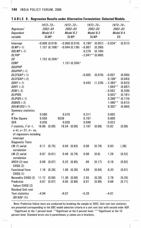
We start here with estimation of equation 9 (the results are presented asmodel B-1 in table 6). Clearly, ED along with lagged inflation appears toexplain a much larger part of current inflation than was the case with theprevious model, and the estimation results are also consistent. However,the coefficient estimates are much too large since they exceed unity, indi-cating the presence of some upward bias possibly involving linkages withomitted variables. Since the normality assumption is violated in model B-1,the significance of the variables was tested using Wald’s maximum likeli-hood criterion. The results indicated that both variables were highly signifi-cant. The rolling regression of lagged inflation is significant, and despiteintermittent failure ED is also significant during most of the windows, par-ticularly the recent period (figure 5).
An alternative and possibly more intuitive way of presenting equation 9is to substitute equation 10 in equation 9 to yield a relationship between thecurrent inflation and the difference between the nominal growth rate andthe real potential growth rate. This difference is represented by the variableEDNP. This regression is presented as model B-2 in table 6. The estimatedcoefficient attaching to EDNP is virtually identical to that associated withED in B-1. The importance of B-2 is that it relates the inflation processdirectly to the difference between the nominal income growth rate and thepotential real growth rate but without imposing any valuation on the latter.The rate of inflation is now a proportion of the excess of nominal incomegrowth over real potential growth. As a consequence the contribution ofthe lagged inflation term is reduced.
Rather than use ED we could use the parallel concept of the change inoutput gap (DGAPHP), which corresponds in growth rate terms to the outputgap earlier employed. When this variable is used in model B-3, the sign issignificantly negative. This is puzzling, given the conventional view that
144 IND IA POL ICY FORUM, 2006
T A B L E 6 . Regression Results under Alternative Formulation: Selected Models
1972–73— 1972–73— 1972–73— 1973–74—Regressor/ 2002–03 2002–03 2002–03 2002–03Dependent Model B-1 Model B-2 Model B-3 Model B-4variable DLWP DLWP DLWP ED
Intercept –0.009 (0.016) –0.009 (0.016) 0.190* (0.057) – 0.034* (0.012)DLWP (–1) 1.157 (0.198)* –0.044 (0.138) –0.067 (0.260)DDLWP (–1) 0.279 (0.194)DLYHP –2.041** (0.960)ED 1.152 (0.204)*EDNP 1.151 (0.204)*DGAPHPDGAPHP (–1)DLCFGAP (–1) –0.055 (0.079) –0.057 (0.050)DLCFGAP (–2) 0.108* (0.043)DDR1 (–1) 0.443 (1.228) – 2.383* (0.623)DDR1 (–2) 1.693** (0.697)DSBI (–2) – 0.552 (0.339)DLIPIG5 0.942* (0.181)DLIPIG5 (–1) 0.366*** (0.174)DGBG5 (–2) 1.480** (0.612)DDLM1DIS (–1) 0.302* (0.064)Summary statisticsR2 0.580 0.570 0.311 0.862R-Bar-Square 0.550 0539 0.167 0.800SER 0.035 0.035 0.048 0.022F statistic, F (k–1, 18.66 [0.00] 18.54 [0.00] 2.167 [0.09] 13.92 [0.00]
n–k), n=31, k= no.of regressors includingintercept
Diagnostic TestsLM (1) serial 0.11 [0.75] 0.04 [0.83] 0.08 [0.78] 0.83 [.36]
correlationLM (2) serial 0.97 [0.61] 0.46 [0.79] 0.08 [0.6] 1.29 [0.52]
correlationARCH (2) test 0.06 [0.97] 0.32 [0.85] .49 [0.17] 0.16 [0.92]
CHSQ (2)Functional Form 1.16 [0.28] 1.06 [0.30] 4.09 [0.04] 6.33 [0.01]
CHSQ (1)Normality CHSQ (2) 11.12 [0.00] 11.30 [0.00] 2.55 [0.28] 2.78 [0.25]Predictive 0.07 [0.97] 0.05 [0.98] 0.01 [0.99] 0.68 [0.71]
failure CHSQ (2)Residual Unit rootTest statistics –4.94 –6.07 –5.20 –4.01
(DF/ADF (1))
Note: Predictive failure tests are conducted by breaking the sample at 2002. Unit root test statisticsare presented corresponding to the SBC model selection criteria in a unit root test with second order ADF.
*Significant at the 1 percent level. **Significant at the 5 percent level. ***Significant at the 10percent level. Standard errors are in parentheses; p values are in brackets.

Sheetal K. Chand and Kanshaiya Singh 145
an increase in the output gap should be more inflationary.14 Such a resultindicates that this view needs to be reconsidered. The fact that a negativesign resulted from regressing the inflation rate on the change in the outputgap suggests that nominal income is determined by a process separate fromthat of its constituents. Hence, since nominal income growth is the sum ofthe inflation rate and the rate of output growth, if the latter increases theformer must decline as long as nominal income is unchanged, which wouldexplain the estimated negative sign.
Next we estimate a reduced-form equation for inflation using equation12 with the specified lag structure and present the results as model B-4.Neither the lagged growth in fiscal deficit nor the lagged change in interest
F I G U R E 5 . Result of Rolling Regression with Variables in Model B-1
14. In a more recent work, the Reserve Bank of India has estimated inflation using theoutput gap and claims to have obtained a positive relationship between the output gap andinflation (RBI 2004). However, this relationship is a very specific case where estimationsare made without intercepts. The results are fragile to inclusion of an intercept term and,therefore, cannot be taken as robust.
146 IND IA POL ICY FORUM, 2006
rate affects current inflation. However, when the same variables are used toexplain ED, they are found to be significant albeit with a different lag struc-ture (model B-5, table 5). The signs are also as expected. The determinantsof ED must be established to identify and quantify the effects of demand-side variables on nominal income, and some testing is undertaken to establishthe influence of additional variables and different lag structures.
Variables that affect ED through the external sector include growth ratesin industrialized countries (DLIPIG5) and changes in GDP-weighted gov-ernment bond yields (DGBG5). Five countries, France Germany, Japan,the United Kingdom, and the United States (G5), are taken to representindustrialized countries. With increasing yield on international bonds, thedomestic currency depreciates, thereby increasing exports. Similarly, withan increase in international output, demand on Indian exports increases.Both these factors lead to an increase in ED.
Looking at domestic financial intermediation, the domestic deposit rate(DR1) and lending rates (SBI) have opposite signs with two lags. A higherdeposit rate indicates liquidity constraint and presumably restrains expend-itures with one lag, while a higher lending rate reduces them with apparentlytwo lags. Concerning monetary and fiscal influences, excess accelerationin narrow money growth (DDLM1DIS) and growth in fiscal deficit(DLCFGAP) are found to significantly affect ED , but with one and twolags respectively. Money growth might itself be affected by the fiscal growthwith a lag, although the two growth rates are not contemporaneously highlycorrelated. In addition the lag structure of the two variables reduces thepossibility of endogeneity. The finding that the first lag of the fiscal variableis not significant need not indicate that fiscal effects are unimportant, butrather that they have not been adequately represented. Aside from the issueof adjusting the fiscal deficit variable to exclude endogeneity effects so asto capture its discretionary aspect, the inclusion of the monetary accelerationterm could primarily reflect fiscal influences, given the dominant role of thebudget in the process of generating the money supply.
Expanding the Alternative Specification
Considering that the inflation models discussed so far have rather limitedexplanatory power and the standard errors of regression are high, it is im-portant to explore other sources of inflation in India. The particular limitationcomes from the adequacy of demand-side variables such as ED in explaininginflation. An alternative approach to modeling the demand side would beto adopt the monetarist way of modeling inflation. In this approach, which

Sheetal K. Chand and Kanshaiya Singh 147
continues to dominate the Indian literature, the price equation is obtainedby inverting the demand for money equation.15 However, a pure demand-type monetarist model can at best provide only a poor and incompletespecification of the inflation process in India, because inflation movementsmay not result simply from excess money over nominal income alone aspredicted by such models. It is revealing that in the annual commentary onprice and distribution in various issues of the Economic Survey, particularlyduring the 1990s, the discussion emphasizes supply-side effects.16 Alsoseveral studies have demonstrated supply-side dominance in the inflationaryprocess in India.17
Nonetheless, even though the supply of money is dominated by the fiscaldeficit and its monetary financing requirements, no model of inflation inIndia can ignore money. This is in keeping with general observations else-where.18 Further, given a desire to collect inflation taxes, the possibility ofsome discretion in conducting monetary policy cannot be ignored. It is alsoimportant to identify a potential monetary aggregate that can be treated asexogenous to the inflationary process. In the current study, narrow money(M1) is identified as the preferred aggregate based on causality tests.
Fewer attempts have been made in recent years in India to address supply-side aspects of price formation behavior involving such variables as nominalwages and prices of important inputs and intermediates at the aggregatelevel. Balakrishnan modeled manufactured prices through an error correctionmodel, using annual data for 1952–80, and found that labor and raw materialcosts were both significant determinants of inflation in the industrial sector.19
Joshi and Little modeled food and nonfood inflation separately using money,consolidated fiscal deficit, food production, nonfood production, and importprices as explanatory variables.20 Callen and Chang modeled WPI-based
15. Pradhan and Subramanian (1998), Arif (1996), and Rangarajan (1998) are threestudies where a predominantly monetarist approach has been used. Most recent amongthese, Pradhan and Subramanian (1998) model the CPI for urban nonmanual workers (CPI-UNME) and the CPI for agricultural labor (CPI-AL), which is dominated by food items.The series on CPI-AL has already been rendered outdated (GOI 1994, 1996), however, andthe CPI-UNME has limited application in conducting monetary policy because of its verysmall basket size, which is focused on a particular segment of the labor force.
16. The Economic Survey is the official document of the Ministry of Finance issuedbefore the presentation of the annual budget of the Government of India.
17. See, for example, Bhattacharya and Lodh (1990) and Singh (2002).18. See, for example, McCallum (1994).19. Balakrishnan (1991, 1992, 1994). Balakrishnan uses a dataset of old vintage that
probably cannot be updated due to discontinuation in data compilation. Therefore, theusefulness of such a study is necessarily limited.
20. Joshi and Little (1994).
148 IND IA POL ICY FORUM, 2006
annual inflation for the period 1957–58–1997–98, with output gaps in in-dustrial and agricultural components of GDP, treating them separately aswell as combined.21 They found that the lagged industrial gap was insignifi-cantly positive, while the lagged agricultural output gap was significantlynegative and the lagged combined output gap insignificantly negative. Thisled them to conclude that inflation in India is structural. They did not analyzethe contemporaneous gaps, however.
Drawing on the above considerations, we adopt the following strategy:First, an input-based basic model is created. This is augmented by addingdemand-side variables in three alternative forms: monetarism, a Phillipscurve output gap analysis, and the alternative ED approach.
A general form of the price equation based on costs can be written asfollows.
(18) ∑∏=
===
n
ii
n
i iiXP
11
1, αµ α
Here, Xi is the cost of the ith factor, α is the share of the ith factor in total costand µ is a constant capturing the markup. Taking logs and then differentiatingyields an input-based inflation equation. In an economywide model, theselection of such variables is limited. Most such inputs may form part ofthe WPI basket. However, we select those sensitive components that areimportant in the production process of several other goods and thus proxya wider range of inputs We consider petroleum mineral oil as a key energysource, and we proxy energy prices using the international price of oil(WOP), as well as the domestic price of mineral oil (WPIMO). DLWOP andDLWPMO represent inflation rates in world oil prices and domestic oilprices. Both variables must be considered because the government of Indiacontrols domestic oil prices using several instruments, and the inflation ratesfor domestic oil prices and world oil prices are not synchronized. However,the world oil price can affect inflation in India through other channels suchas the international prices of goods and services, the transport cost of Indianexports, and expectations about future prices.
To capture agriculture-specific effects, we choose the price of fertilizer(WPIFZ) as another key input. Edible oil (WPIEO) is considered as a criticalinput to manufactured food. The weights of mineral oil, edible oil, and
21. Callen and Chang (1999) also model quarterly inflation using an index of industrialproduction–based output gap and report signs of the output gap term that are not consistentwith standard expectations.

Sheetal K. Chand and Kanshaiya Singh 149
fertilizer in the overall WPI are about 6.7 percent, 2.5 percent, and 3.9 per-cent, respectively. The weight of manufactured goods is 63.8 percent; thatof fuel, power, and lubricants is 14.2 percent; food products, 15.4 percent;and nonfood primary products including minerals, 6.6 percent.
Edible oil inflation, which is part of the manufacturing sector, is nothighly correlated with inflation in that sector, partly because a substantialpart of it is imported. In line with expectations, mineral oil and edible oilprice inflation are not themselves correlated (appendix table A-2). Therefore,both can be allowed in the inflation model as supply-side variables, wherethey proxy a sensitive component of import prices in India.22 In addition,we also use world consumer price inflation (DLCPIW), as reported by theInternational Monetary Fund in its International Financial Statistics, tocapture the general inflation trend worldwide. The sign of DLCPIW is pos-itive and significant, indicating the wider interaction of the Indian economywith the rest of the world.
Regarding wage price inflation, wages of public sector employees(WAGPI) are used as the benchmark salary for workers in other sectors, sinceIndia has no series to represent general wage price inflation. However, publicsector wages are likely to influence the wages elsewhere in the economyand so considered a suitable proxy for wage inflation at the aggregate level.
Finally, to see if it provides a suitable hybrid, money is introduced intomodel C-2 as excess money growth over its long-term trend growth rate(DLM1DIS). Treating money in this way yields the same coefficients withor without the long-term trend growth The advantage of this definition,however, is that it corresponds better to the meaning of discretionary moneygrowth. In addition, the selection of narrow money is motivated by the find-ing that this aggregate precedes inflation in the sense of Granger causality,while other aggregates have bidirectional causality. Although the introduc-tion of money in model C-2 improves the model significantly, the coefficientsof monetary growth are small at 0.35 including both lags, a finding thatindicates that the scope for purely monetary control on inflation is limited,at least in the short run (table 7).
Table 8 incorporates the two additional and alternative specifications ofthe demand side in the basic supply-side platform. Model D-1 clearly indi-cates the supply dominance on the economy’s inflation rate. Most of thesupply-side variables remain significant. While contemporaneous as wellas lagged DGAPHP remains negative, however, the size of the coefficientsis reduced significantly. All the variables contained in model C-1 retain their
22. Singh (2002).

150 IND IA POL ICY FORUM, 2006
signs as well as size. The model D-1 is statistically well estimated withhigh R2 and good forecasting ability, but the size of the demand-side effectsis difficult to know because the sign of DGAPHP is negative.
Model D-2 is obtained by superimposing input price inflation rates ondemand-side effects captured in ED. The coefficient of ED is positive andhighly significant, but its size is reduced from the one obtained in modelB-1, which was excessive. The R2 is more than 0.90, but the model is notacceptable statistically because of the problem of serial correlation in errors.Model D-2 can be augmented in a number of ways, as indicated in table 8,by including more variables such as deviations in rainfall (DRAIN) andgrowth in foreign exchange reserves (DLFERU). Inclusion of these variables
T A B L E 7 . Regression Results of Input-Based Inflation Models: Selected Models
1972–73—2002–03 1972–73—2002–03Model C-1 Model C-2
Regressor/Dependent variable DLWP DLWP
Intercept 0.107 (0.013) 0.027*** (0.014)DLWAGEPI 0.018 (0.063) 0.020 (0.061)DLWFZ 0.113** (0.049) 0.108** (0.046)DLPEO 0.175* (0.034) 0.159* (0.035)DLPMO 0.115*** (0.061) 0.129** (0.057)DLWOP 0.040** (0.016) 0.038** (0.014)DLCPIW 0.230* (0.081) 0.123 (0.086)DLM1DIS 0.150** (0.073)DLM1DIS (–1) 0.155*** (0.076)
Summary statisticsR-Square 0.858 0.889R-Bar-Square 0.822 0.850S.E of Regression 0.022 0.020F statistic, F (k–1, n–k), n=31, k= no. 24.16 [0.00] 22.10 [0.00]
of regressors including interceptDiagnostic TestsLM (1) serial correlation 0.03 [0.87] 0.05 [0.83]LM (2) serial correlation 4.15 [0.13] 4.20 [0.12]ARCH (2) test CHSQ (3) 0.92 [0.63] 1.30 [0.52]Functional Form CHSQ (1) 0.30 [0.58] 0.57 [0.45]Normality CHSQ (2) 0.41 [0.82] 2.46 [0.29]Predictive failure CHSQ (2) 0.35 [0.84] 0.69 [0.71]Residual Unit rootTest statistics (DF) –4.94 –4.99
Note: Predictive failure tests are conducted by breaking the sample at 2002. Unit root test statistics arepresented corresponding to the SBC model selection criteria in a unit root test with second order ADF.
*Significant at the 1 percent level. **Significant at the 5 percent level. ***Significant at the 10 percentlevel. Standard errors are in parentheses; p values are in brackets.

Sheetal K. Chand and Kanshaiya Singh 151
T A B L E 8 . Regression Results of Hybrid Inflation Models with Demand- andSupply-Side Variables: Selected Models
1972–73— 1972–73— 1972–73— 1972–73—Regressor/ 2002–03 2002–03 2002–03 2002–03Dependent Model D-1 Model D-2 Model D-3 Model D-4variable DLWP DLWP DLWP DLWPIntercept 0.008 (0.012) –0.025 (0.011) –0.043* (0.013) –0.042* (0.009)DLWP (–1) 0.294***(0.161) 0.840* (0.131) 0.693* (0.196) 1.032* (0.113)ED 0.517* (0.162) 0.797* (0.142) 0.722* (0.195) 0.932* (0.118)DGAPHPDGAPHP (–1)DLWAGEPI 0.012 (0.054) 0.093** (0.042) 0.101*** (0.054) 0.102**(0.037)DLWFZ 0.158* (0.038)DLPEO 0.095** (0.038) 0.082* (0.031) 0.100** (0.040) 0.066* (0.027)DLPMO 0.078 (0.053) 0.152** (0.031) 0.180* (0.039) 0.161* (0.025)DLWOP 0.035** (0.013) 0.013 (0.010) 0.028* (0.014)DLCPIW 0.148***(0.080) 0.173** (0.082)DLM1DIS 0.207* (0.046)DLM1DIS (–1) 0.121** (0.053)DRAINR –0.115* (0.032) –0.087*** (0.044) –0.111* (0.030)DLFERU 0.034* (0.013) 0.036** (0.016) 0.033* (0.011)DDLM1DIS 0.161* (0.031)DDLM1DIS (–1) 0.191* (0.033)
Summary statisticsR-Square 0.906 0.949 0.912 0.963R-Bar-Square 0.870 0.923 0.879 0.947S.E of Regression 0.019 0.014 0.018 0.012F statistic, F(k–1, 26.42 [0.00] 37.29 [0.00] 27.26 [0.00] 58.50 [0.00]
n–k), n=31,k= no.of regressorsincluding intercept
Diagnostic TestsLM (1) serial 2.87 [0.09] 0.74 [0.38] 0.91 [0.98] 0.01 [0.93]
correlationLM (2) serial 8.20 [0.02] 1.89 [0.38] 5.90 [0.05] 0.88 [0.65]
correlationARCH (2) test 1.13 [0.57] 0.67 [0.72] 2.19 [0.35] 0.46 [0.79]
CHSQ (2)Functional Form 0.62 [0.43] 0.00 [0.95] 0.26 [0.61] 2.95 [0.09]
CHSQ (1)Normality CHSQ (2) 3.13 [0.21] 1.01 [0.60] 3.13 [0.21] 0.99 [0.61]Predictive failure 0.20 [0.91] 2.89 [0.24] 0.21 [0.90] 1.57 [0.46]
CHSQ (2)Residual Unit rootTest statistics –6.62 –5.62 –5.31 –5.25
(DF/ADF(1))Note: Predictive failure tests are conducted by breaking the sample at 2002. Unit root test statistics are
presented corresponding to the SBC model selection criteria in a unit root test with second order ADF.*Significant at the 1 percent level. **Significant at the 5 percent level.***Significant at the 10 percent
level. Standard errors are in parentheses; p values are in brackets.

152 IND IA POL ICY FORUM, 2006
improves the explanatory and predictive power of the models. It may benoticed that DRAIN and DLFERU are also supply-side variables, whichare observed to be significant with appropriate signs only in the presenceof demand-side variables and the lagged inflation. These variables did notimprove the results for the models shown in table 5. Therefore, they couldbe considered to be conditionally significant. Also, in models D-3 and D-4,we removed DLWFZ (fertilizer price inflation) in favor of oil price inflationto improve the model specification. The fertilizer price could be partly deter-mined by the oil price, which is one of the key inputs and also by weatherconditions (during favorable weather, farmers are tempted to use more in-puts, which raises the fertilizer price).
Adding these additional variables improves the statistical properties.Therefore, on statistical grounds we select model D-3 for further analysisand run a rolling regression for all the variables on the right-hand side tak-ing a window size of 20, which is reasonable given the number of variablesin the model. The results of the rolling regression are presented in figure 6.Clearly, contemporaneous money growth, edible oil price inflation, mineraloil price inflation, ED, lagged inflation, and wage price inflation remainsignificant.
A Strategy for Controlling Inflation in India
The empirical results discussed in this paper indicate that the determinationof the inflation rate in India does not correspond to the stylized profile ofthe demand-dependant Philips curve trade-off prevalent in the advancedeconomies, or to the associated use of the nominal interest rate as the chiefinstrument with which to influence the inflation rate. Nor did the monetaristmodel perform well. An alternative model was developed to better portraydemand-side effects on inflation, while allowing for supply-side phenomena.This model performed much better under conditions prevailing in India.The estimation results indicate that the transmission lag between the ex-penditure stimulus, represented by the excess demand variable ED, and theinflation rate is quite short. This finding suggests a more active use ofdemand-management policy in inflation control, for example, through theuse of fiscal policy, since it is more feasible to adopt and maintain a fiscalstance that is geared to projected developments a year ahead than for, say,two or more years.

Sheetal K. Chand and Kanshaiya Singh 153
F I G U R E 6 . Rolling Diagrams of Regression for Model D-3: DLWP on INPT,DLWP [1], ED [0], DLPEO [0], DLPMO [0], DLWOP, DLM1DIS[0-1], DRAIN[0],DLFERUWB [0], and DLWAGPI [0]
(Figure 6 continued)

154 IND IA POL ICY FORUM, 2006
(Figure 6 continued)
(Figure 6 continued)

Sheetal K. Chand and Kanshaiya Singh 155
(Figure 6 continued)
(Figure 6 continued)

156 IND IA POL ICY FORUM, 2006
(Figure 6 continued)
(Figure 6 continued)

Sheetal K. Chand and Kanshaiya Singh 157
(Figure 6 continued)
An issue that needs to be clarified is that of the determinants of ED. Forestimation purposes we assumed that fiscal effects could be captured bythe unadjusted fiscal deficit. The results obtained did not bear this out.More research will be needed to identify precisely how fiscal instrumentsaffect aggregate demand. In particular, a fiscal measure is required that

158 IND IA POL ICY FORUM, 2006
separates out feedback effects of the economy on the budget. Under Indianinstitutional conditions, it seems likely that fiscal effects are being capturedby the growth in M1—for which budget deficit financing requirements areprominent—in a context of interest rate restraint.
In any case, given the size of the fiscal deficit and its undoubted stimulusand crowding out effects, one component of the suggested approach toinflation targeting in the Indian context would be to rely more on fiscalrestraint. If the forecast rate of inflation is likely to exceed the target rate,both the fiscal deficit and its monetary financing would need to be reduced.Of course, simply reducing the monetary financing would not be adequate,either because with unchanged interest rates the increased supply of govern-ment paper would be monetized, or because interest rates would increaseand some private sector crowding out would occur through that channel.
It is also apparent that safeguards would need to be built in to ensurethat political expediency does not lead to a watering down of the commitmentto restrain inflation. India has adopted the Fiscal Responsibility and BudgetManagement Act, which is expected to ensure fiscal discipline. That laweases the concern that relying on fiscal instruments is more open to short-term political expediency. It may still be necessary to develop further themechanisms for ensuring sound fiscal policy. A simple way to achieve thisis to require that the government and the central bank agree on the size ofthe fiscal deficit and the amount of permissible monetary financing. If theagreement cannot be upheld, then the central bank would be free to raiseinterest rates.
Another component of ED is private expenditures, which in an expend-iture approach to inflation control may also need to be restrained. Usingthe interest rate for this purpose may not be advisable if it has undesirableside effects; for example, the exchange rate could appreciate in a persistentmanner that damages export prospects and leads to excessive imports. Assetvaluations could become so depressed that long-lasting adverse effects oncapital accumulation are created. Regulating the flow supply of credit thatfinances investment expenditures by adjusting liquidity ratios may be moreappropriate, especially since that approach is likely to have weaker, lessdirect adverse effects on stock asset valuations.
Abstracting from an active use of the interest rate for purposes of inflationcontrol raises the issue of what role the Reserve Bank of India (RBI) wouldplay, aside from regulating liquidity ratios? A useful application would in-volve portfolio side operations. A key objective for portfolio operationswould be to maintain a desired real interest rate, with the nominal interestadjusted whenever the underlying inflation rate deviates from target. From

Sheetal K. Chand and Kanshaiya Singh 159
time to time, shifts in liquidity preferences result in asset transactions thateither press interest rates above or below the target long-term level. Accom-modating liquidity preference shifts through appropriate open market oper-ations helps keep interest rates stable. If, for example, interest rates were tobe reduced to very low levels, there would be at least two effects: first, thereward from postponing consumption would be reduced, which would tendto stimulate current consumption, and second, the discount factor used inestablishing the present values of assets would be lowered, which wouldincrease asset values and could have undesirable distortions on the goodsmarket.
In this connection, some recent institutional changes affecting the oper-ations of the RBI are of interest. The inflow of remittances and foreign insti-tutional investors has added to the foreign exchange reserves at an averageannual rate of about 18 percent during the last ten years. Concerned overpossible currency appreciation and potential adverse effects on exports, theRBI has been undertaking heavy sterilization, with the result that its holdingsof domestic assets are almost depleted. A new instrument called a marketstabilization scheme (MSS) has now been implemented, whereby the RBIprints money that is kept in a sterilized government account, and pays intereston the equivalent Treasury bills to buy foreign exchange assets from thedomestic market. This maneuver enables the RBI to restrain appreciation,but at the cost of keeping interest rates above international levels, the currentwedge being about two percentage points. This, of course, tends to attractcapital inflows, given the market’s perception that the RBI will keep ex-change rates stable, which then requires some further sterilization andreserve accumulation. A potential for conflict thus exists between interestrate levels that are better geared to internal requirements and those neededas a consequence of international considerations. One way of resolving theconflict would be to apply regulatory and control devices of various sortsto prevent excessive capital inflows.
Conclusion
Key support for the inflation-targeting framework has emerged from twoimportant experiences. First, financial sector reforms and globalization haveled to the breakdown of the broad money demand equation in several coun-tries, including India, which has rendered monetary targeting less reliable.The second key reason has been a broader agreement worldwide on main-taining a lower level of inflation as it is detrimental to sustainable growth

160 IND IA POL ICY FORUM, 2006
for various reasons including uncertainties in investment and savingsbehavior.
The advantage of the ITF is the direct relationship between the inflationtarget and the objective of monetary policy. However, there is an importantquestion about the efficacy of monetary instruments in targeting inflation,especially in the case of developing countries where a number of rigiditiespersist because of direct and indirect controls and constraints. The economymay not fully employ its resources and the concept of a nonacceleratingrate of unemployment may not apply. The supply-side dominance appearssufficiently prominent that monetary stance, which relies on influencingthe demand side, may be a misjudged risky option. Monetary policy mayend up tightening the supply too much, or it may be too proactive, adverselyaffecting current income flows. Furthermore, it carries potential asset andbalance sheet valuation effects that could be disruptive, in addition to adversereal exchange rate developments.
Even advanced economies have been exposed from time to time to costlyconsequences from persistent deviations of interest and exchange rates fromequilibrium levels, and from increased volatility. For example, the realappreciation of the euro by almost 60 percent against the dollar in recentyears is an important factor in the erosion of competitiveness and the sluggisheconomic performance that much of Europe is experiencing today. Eventhough interest rates are low in Europe, with the European Central Bankessentially operating as an inflation targeter, rates have been even lower inthe United States. In addition, for some time now, prospective inflationrates have appeared to be well below target, spawning a “fear of deflation”syndrome that has led to an unprecedented lowering of nominal interestrates in several advanced economies.23 The low interest rates in turn havecontributed to an excessive upward revaluation of assets in these economies,including especially real estate, where low rates appear to have fueled a
23. The concern with deflation is understandable in an economy, such as Japan’s, thathas experienced a long period of stagnation. However, it is more difficult to explain theseconcerns in such economies as the United States, the United Kingdom, or even Australia,since they are, or have been, booming. The unexpectedly benign inflation performanceappears to have contributed to this fear of deflation and led to historically low interestlevels as inflation targeting would counsel. There is an asymmetry when monetary authoritiesavow that they are able to identify a deflationary prospect but not an inflationary asset pricebubble. Nonetheless, the deflationary reading may have been inappropriate, which illustratesthe importance of distinguishing between supply shocks to inflation—productivity growth,the “China factor,” or appreciating exchange rates—and demand-side shocks. The fact that theaforementioned economies have simultaneously run very large current account deficits ontheir balance of payments suggests that demand pressures were potentially inflationary butwere dissipated through higher imports, especially from China.

Sheetal K. Chand and Kanshaiya Singh 161
less productive investment boom in that area, while excessively stimulatingconsumption. On occasion regulatory facilities have also been found want-ing, as evidenced by the Long-Term Capital Management Hedge Fund crisisor recent concerns that hedge funds are too lightly regulated.
A more cautious approach to inflation targeting in India would rely onboth monetary and fiscal instruments and be closely coordinated with otherinstruments such as government buffer stock and other supply-side oper-ations. If the forecast rate of inflation were to exceed the target rate, both thefiscal deficit and its monetary financing and the general availability of creditflows would be reduced, but without necessarily raising real interest rates.Of course, safeguards would need to be installed to ensure that political ex-pediency does not lead to a watering down of the commitment to restraininginflation.
Appendix. List of Variables and Their Descriptions
CGAP Combined gap between outlay and revenue (Rs mn).CPIG5 Consumer Price Index for trade-weighted geometric mean of G-5 countries. Base:
1993–94.CPIW Consumer Price Index for world. Converted Base: 1993–94.DR1 One-three year commercial bank deposit rates (percent per year).DRAINR Variation of actual rain fall from normal (fraction).DSBI sbi-sbi(–1)ED dlyn–[(1+dlwpl)*(1+dlyhp)–1]FERURB Foreign exchange reserves, including gold (current US$ mn).FERUWB Gross international reserves, including gold (current US$ mn).GAPHP ly –lyhp.GBG5 International government bond (GB)rates. Average of the monthly (line 61 of IFS).INPT InterceptIPIG5 Industrial production index of G5 countries (trade-weighted geometric mean).LYHP hpf(ly, 7).LYNHP hpf(lyn, 7).M1 Narrow money M1 (Rs mn).RGDP GDP at market prices, in constant 1993–94 prices (Rs. mn).SBI Average lending rate of State Bank of India (percent per year).T Time trendUSGB U.S. government bond yield (percent per year). Source: IFS: M111.61WAGPI Index of per capita remunerations of public sector employees (1993=100).WOP World oil (crude) price index. Converted Base: 1993–94=100. Source: IFS.WPI World price index of all commodities at 1993–94 prices. Source: ES.WPIEO WPI for edible oil (domestic).WPIFD WPI for primary food (domestic).WPIFZ WPI for fertilizer (domestic).WPIMO WPI for mineral oil (domestic).Y GDP at market prices, in constant 1993–94 prices (Rs. mn).YN GDP at market prices, in current LCU (Rs. mn).

162 IND IA POL ICY FORUM, 2006
TA
BL
E A
-2.
Stat
istic
al P
rope
rtie
s of
Sel
ecte
d Va
riabl
es, 1
972–
2004
Std.
Coef
. of
Unit
root
Varia
ble(
s)M
axim
umM
inim
umM
ean
Devi
atio
nSk
ewne
ssKu
rtos
is-3
varia
tion
test
a
DLW
P0.
2247
–0.0
109
0.07
620.
0507
1.04
841.
1452
0.67
–4.4
1ED
0.07
16–0
.200
0–0
.002
80.
0487
–1.8
686
6.32
1717
.46
–5.8
6DL
PEO
0.40
21–0
.242
20.
0747
0.13
41–0
.198
50.
1058
1.79
–7.6
6DL
PMO
0.52
480.
0000
0.10
580.
1134
1.92
084.
1505
1.07
–4.7
4DL
WOP
0.85
20–0
.550
80.
0878
0.30
700.
7943
0.81
143.
50–4
.23
DLM
1DIS
0.10
34–0
.247
4–0
.007
10.
0602
–1.7
212
5.95
658.
48–6
.93
DRAI
NR0.
1617
–0.2
472
–0.0
353
0.10
57–0
.248
6–0
.637
72.
99–7
.42
DLW
AGPI
0.28
38–0
.040
80.
1178
0.07
72–0
.043
40.
2544
0.66
–6.5
3DL
FERU
WB
0.59
12–0
.392
80.
1408
0.23
28–0
.296
8–0
.100
71.
65–3
.81
DGAP
HP0.
0490
–0.0
871
–0.0
001
0.02
46–1
.134
63.
2304
364
–8.0
5DL
CPIW
0.24
430.
0327
0.11
860.
0565
0.06
18–0
.703
20.
48–1
.47
DLW
PFZ
0.57
70–0
.139
50.
0646
0.13
562.
0055
4.94
812.
10–4
.47
a. C
ritic
al v
alue
at 5
per
cent
= 2
.99.
DLC
PIW
dem
onst
rate
s a
stru
ctur
al b
reak
at 1
994–
96 w
hen
infla
tion
falls
from
pre
viou
s hi
gh le
vels
of a
roun
d 20
per
cent
to lo
w le
vels
of a
roun
d 5
perc
ent a
fter
199
6.

Sheetal K. Chand and Kanshaiya Singh 163
Tabl
e A-
3. C
orre
latio
n M
atrix
of t
he S
elec
ted
Varia
bles
, 197
2–20
04
DLW
PED
DLPE
ODL
PMO
DLW
OPDL
M1D
ISDR
AIN
DLW
AGPI
DLFE
RUW
BDG
APHP
DLCP
IWDL
WPF
Z
DLW
P1.
00ED
0.22
1.00
DLPE
O0.
570.
541.
00DL
PMO
0.66
–0.1
80.
071.
00DL
WOP
0.49
0.15
0.14
0.48
1.00
DLM
1DIS
0.06
0.09
0.00
–0.1
5–0
.12
1.00
DRAI
N–0
.15
0.01
–0.1
4–0
.14
–0.2
50.
191.
00DL
WAG
PI0.
12–0
.36
–0.3
70.
320.
09–0
.19
0.12
1.00
DLFE
RUW
B0.
050.
260.
090.
020.
180.
07–0
.17
–0.1
81.
00DG
APHP
–0.3
5–0
.29
–0.2
6–0
.17
–0.3
0–0
.20
0.66
0.14
–0.3
51.
00DL
CPIW
0.44
–0.0
40.
180.
090.
000.
240.
240.
16–0
.24
0.00
1.00
DLW
PFZ
0.65
–0.4
10.
100.
740.
16–0
.05
–0.1
30.
400.
07–0
.05
0.28
1.00

164
Comments and Discussion
Rajnish Mehra: The authors, whose analysis builds on their earlier work,have produced a thought-provoking paper.1 They highlight many interestingissues regarding the policy implications of inflation targeting and drawupon the experience of countries that have adopted this framework. I do,however, take issue with the methodology of the study—that of testing anatheoretical model on historical data and then using it for policy analysis.My specific comments on the paper appear at the end of this discussion.
I begin by focusing on some of the issues raised in the paper and bymaking a distinction between targeting inflation and inflation targeting.
Targeting Inflation
The rational for targeting inflation is the lesson learned over the past threedecades, about which there is broad consensus, that positive expectedinflation, above some low rate, is welfare reducing
There is less agreement on how this low inflation state should be achieved.In the late 1960s, the prevailing view, championed by Paul Samuelson andRobert Solow, advocated the use of control theory for formulating and imple-menting macroeconomic policy. A minority, notably Milton Friedman,argued against this, claiming that policy acted with long, variable, andunpredictable lags. With the advent of the Lucas Critique and the Time-Inconsistency literature, the later view has gradually prevailed.2
Today, most academics and policymakers accept the view that the econ-omy is complex and that control theory is inappropriate for macroeconomicstabilization. It is also the view, articulated by Friedman and Phelps, thatthere is no long-run Phillips-curve trade-off.3
I specially thank Henning Bohn, Barry Bosworth (the editor), John Donaldson, andEdward Prescott for their insightful comments. I am grateful to the participants of the IndiaPolicy Forum Conference for a stimulating discussion.
1. See, in particular, Chand (1977), McKibbin and Singh (2003), and Singh and Kalirajan(2003).
2. Kydland and Prescott (1977).3. Friedman (1968); Phelps (1968).

Sheetal K. Chand and Kanshaiya Singh 165
Whether there is indeed a short-run Phillips-curve relationship andwhether monetary policy can beneficially exploit this short-run trade-offbetween inflation and the output gap is a long-standing dispute that is stillat the center of monetary policy discussions. Friedman and Lucas haveargued that given the inherent complexity of the economy and our incompleteknowledge of it, monetary policy should be limited to achieving nominalstability. Their arguments are based on the view that although monetarypolicy has strong short-run real effects, there is no way to exploit thembeneficially. They suggest that a response in the form of a k-percent rulefor money growth is the best way to achieve nominal stability. Svenssonand Woodford on the other hand, argue that there are (limited) short-run ex-ploitable trade-offs.4 In their analysis, they describe a framework involvingoptimal exploitation of the short-run trade-off.
Irrespective of one’s position on the issues discussed above, the rationalfor targeting inflation is clear. Lower inflation rates lead to better operatingcharacteristics for the economy. See, for example, figure 7, which plots thereal growth of gross national product versus inflation for India for thepostwar period.
F I G U R E 7
4. Svensson (1999); Svensson and Woodford (2004).

166 IND IA POL ICY FORUM, 2006
Inflation Targeting
What is inflation targeting? This is not an easy question to answer as thereare many variations on the theme. As broadly accepted, it is a frameworkfor monetary policy whereby a short-term interest rate instrument respondsto deviations of expected future inflation from the target rate and to devi-ations of output from its full-employment level. It explicitly incorporatesthe type of Phillips-curve trade-off discussed earlier. An important featureof inflation targeting is the articulation of this policy—to clearly communi-cate to the public the plans and objectives of the monetary authorities. Thisis intended to serve as a quasi-commitment mechanism.
One variant—“the hard version”— is the original Svensson framework.5
It argues that the central bank should concentrate only on inflation to theexclusion of any other objectives. There are a host of other variations—“the soft versions”—with inflation as only one of the targeted variables. Thevariants differ depending on what is included in the targeted set. Informalconversations with central banking officials in a number of countries leadme to believe that inflation targeting in practice is almost never implementedin its hard version.
Several questions must then be addressed before a soft version can beeffectively implemented. The policymaker must not only articulate the re-lative weights to attach to inflation and output and specify the horizon forexpected inflation and output but must also explicitly address the issue ofwhat variables, other than expected inflation and the output gap, are to betargeted. Thus, inflation targeting in practice targets inflation as well asthe output gap, interest rate fluctuations and perhaps other macroeconomicvariables as well.
Although many of its proponents, including Svensson, call it a rule, inthe face of multiple objectives, it is a discretionary policy with the Phillipscurve as its deus ex machina. Its implementation (especially in the face ofmultiple objectives) will be plagued by all the issues associated with “themulti-period control problem under uncertainty.”6
Crucial to its success is the issue of credibility and managing expectations.The more objectives that are targeted, the less credible will be the commit-ment to target inflation since some of these objectives may be mutuallyinconsistent. I revisit this issue in the next section.
5. Svensson (1997). Henning Bohn suggested this “hard version” usage, which is theversion “tested” by the authors in the paper.
6. By postulating a specific lag structure, Svensson and others convert the multiperiodproblem to a sequence of static problems and circumvent some of these issues and theirimplications.

Sheetal K. Chand and Kanshaiya Singh 167
There is little doubt that a central bank can control inflation. This control,though not perfect due to macroeconomic shocks (such as oil supply shocks)involves costs, which may not be (politically) acceptable. Economic agents,of course take this into account when forming their expectations.
The United States does not explicitly target inflation; in contrast, Canadaand the United Kingdom are explicit inflation targeters. 7 In all three countriesinflation is low, but it is difficult to attribute this categorically to ITF pro-grams. Ball and Sheridan examine a sample of twenty industrialized coun-tries, seven of which are targeters and thirteen nontargeters.8 They concludethat on a number of dimensions there is no evidence that inflation targetingimproves economic performance. Others, notably Bernanke, King, Mishkin,Svensson and several central bankers (of course!) beg to differ. In the absenceof credibility, inflation targeting is just another value-loaded term (with apositive valence).
The Indian Context
Implementing inflation targeting in India raises a number of issues, sometechnical, others more serious, which address credibility. These include:
– India lacks a comprehensive price index that adjusts for quality andtechnical innovation. This “measurement issue” could be a majorimpediment to implementing inflation targeting effectively. Currentestimates are most likely upwardly biased.
– What is the evidence on the Phillips curve in India, given the structureof the labor force?
– To what extent will the policy of pegging the rupee to the dollarundermine the credibility of a central bank that promises to inflationtarget? Pegging the currency and inflation targeting are not in general,mutually consistent. If an inflationary shock mandates high rates inthe one country, while low rates persist in the other, capital will flowto the high-rate country, putting pressure on the currency peg. Topeg the rupee to the dollar, the Reserve Bank of India has engaged ina classic sterilization policy, buying foreign currency and bonds andoffsetting these purchases by selling domestic bonds. Given that thedomestic assets of the RBI are rapidly being depleted, it is only a
7. With Bernanke’s appointment as the Chairman of the Federal Reserve, this willprobably change as, unlike his predecessor, Bernanke has long supported the concept; see,for instance, Bernanke (1999). It should be noted that by law the Federal Reserve is mandatedto pursue maximum employment.
8. Ball and Sheridan (2003).

168 IND IA POL ICY FORUM, 2006
matter of time before the monetary base will be affected—with theconcomitant effect on inflation.
– What is the role of current asset valuation levels? Inflation targetingin its hard version also precludes intervening in asset markets in caseof a bubble. As Bernanke and Gertler emphasize: “Importantly, italso implies that policy should not respond to changes in asset prices,except in so far as they signal changes in expected inflation.”9 Assetvaluations in India are at an all-time high. The Indian stock markethad risen by more than 90 percent between June 2004 and June 2005and continues to rise. Figure 8 illustrates this dramatic increase invaluation. The 15 percent decline in the stock index on May 17, 2004,surely had information content regarding fundamental valuations!Again this raises the issue of credibility.
– What about taxation. Given a large parallel economy and politicalconsiderations that preclude the taxation of certain sectors of theeconomy such as agriculture, an inflation tax may be a necessary evil.There is always a temptation for governments to let inflation exceedexpectations and needless to say the populous is aware of this!Credibility issues once again are at the forefront of concern.
F I G U R E 8 . Market Value of Equity in the Indian Stock Market
9. Bernanke and Gertler (1999).

Sheetal K. Chand and Kanshaiya Singh 169
Inflation in India is currently running at about 5.6 percent with GDPgrowth at a healthy 8 percent. The current environment is ideal for embarkingon an inflation targeting program. In the absence of a comprehensive priceindex, the core CPI should be targeted after allowing for a bias in measure-ment of, say, 1 percent. An advantage of this is that it avoids potentiallydestabilizing policy responses. The credibility issues raised above wouldhave to be addressed in a transparent manner. The challenge would be toarticulate a policy that is credible but not vacuous.
Comments and Quibbles
The paper addresses many, sometimes orthogonal, issues. This is both astrength and a weakness. On the positive side, it alerts the reader to a hostof interesting questions; on the other hand, at times it appears to lack aunifying theme.
The paper starts out by “testing” a reduced form of the Svensson model.The authors conclude it does poorly when confronted with Indian data (seetable 5). The authors then propose two alternative models: the first focuseson excess demand, where they essentially replace the output gap in theSvensson model with the fiscal deficit. The other is an input-based supply-side model that examines industrial commodities and their price effects onoverall inflation. These extensions are completely ad hoc and atheoretical.The authors provide no justification, either empirical or theoretical, fortheir formulations. In fact the “excess demand” model is a radical changeof the Svensson formulation—a change from “levels” to “growth rates.”They find that these alternatives are an improvement in the sense that certaincoefficients are “significant.” I disagree with this as a research methodologyespecially for formulating policy.
Their key conclusion is that in the Indian context, the use of fiscal policyrather than monetary instruments is likely to be more effective in controllinginflation.
I remain skeptical. To quote Friedman, “Inflation is always and every-where a monetary phenomena.” The effectiveness of policies predicated onusing fiscal instruments is an open question. The fiscal deficit is a far moredifficult policy instrument to control—quickly and smoothly—than aremonetary instruments. While the coordination of fiscal and monetary policymay sound good in theory, it can lead to undesirable outcomes since thesepolicies act with differing lags and over different time intervals. The formu-lation in the paper implicitly assumes that these time intervals are identical.
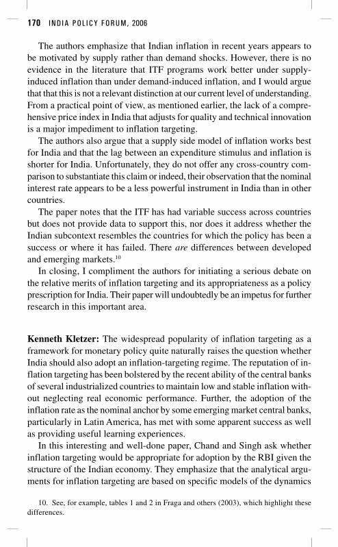
170 IND IA POL ICY FORUM, 2006
The authors emphasize that Indian inflation in recent years appears tobe motivated by supply rather than demand shocks. However, there is noevidence in the literature that ITF programs work better under supply-induced inflation than under demand-induced inflation, and I would arguethat that this is not a relevant distinction at our current level of understanding.From a practical point of view, as mentioned earlier, the lack of a compre-hensive price index in India that adjusts for quality and technical innovationis a major impediment to inflation targeting.
The authors also argue that a supply side model of inflation works bestfor India and that the lag between an expenditure stimulus and inflation isshorter for India. Unfortunately, they do not offer any cross-country com-parison to substantiate this claim or indeed, their observation that the nominalinterest rate appears to be a less powerful instrument in India than in othercountries.
The paper notes that the ITF has had variable success across countriesbut does not provide data to support this, nor does it address whether theIndian subcontext resembles the countries for which the policy has been asuccess or where it has failed. There are differences between developedand emerging markets.10
In closing, I compliment the authors for initiating a serious debate onthe relative merits of inflation targeting and its appropriateness as a policyprescription for India. Their paper will undoubtedly be an impetus for furtherresearch in this important area.
Kenneth Kletzer: The widespread popularity of inflation targeting as aframework for monetary policy quite naturally raises the question whetherIndia should also adopt an inflation-targeting regime. The reputation of in-flation targeting has been bolstered by the recent ability of the central banksof several industrialized countries to maintain low and stable inflation with-out neglecting real economic performance. Further, the adoption of theinflation rate as the nominal anchor by some emerging market central banks,particularly in Latin America, has met with some apparent success as wellas providing useful learning experiences.
In this interesting and well-done paper, Chand and Singh ask whetherinflation targeting would be appropriate for adoption by the RBI given thestructure of the Indian economy. They emphasize that the analytical argu-ments for inflation targeting are based on specific models of the dynamics
10. See, for example, tables 1 and 2 in Fraga and others (2003), which highlight thesedifferences.

Sheetal K. Chand and Kanshaiya Singh 171
of inflation and aggregate output fluctuations and that the nominal interestrate takes the central role as the instrument of monetary policy. The primaryargument of Chand and Singh is that the basic assumptions of themacroeconomic models used to motivate a monetary policy regime targetinginflation with interest rate instruments fail to match the dynamics of inflationand output growth in India. Certainly, the empirical evidence presented inthe paper demonstrates the poor relationship of the inflationary processunderlying monetary policy analysis in advanced industrialized countriesto the macroeconomic data for the Indian economy.
Much of the analysis and criticism of applying inflation targeting inemerging markets centers on countries with open capital accounts, raisingconcerns about the conflicting objectives of price level stabilization andnominal exchange rate stabilization, as well as the consequences of inflationstabilization for interest rate volatility. Chand and Singh raise these issuesin their argument that India is not a good candidate for an inflation-targetingframework for monetary policy. At the same time, proponents of inflationtargeting often emphasize the importance of building credibility aroundannounced inflation goals in emerging market economies as several emer-ging market governments have adopted inflation-targeting regimes withvarying degrees of discretion. Rather than reiterate the credibility question,Chand and Singh concentrate on the modeling issue—how does the in-flationary and real growth process work in India.
In contrast with most emerging market economies that are candidatesfor inflation-targeting monetary regimes, India restricts international capitalflows and has not liberalized financial capital outflows to any significantextent. An important and open question concerns the appropriate monetarypolicy framework for India in anticipation of further liberalization of theeconomy and integration with international financial markets. The motivat-ing issue for the Chand and Singh paper is the analysis of appropriate choicesof monetary policy rules for the Indian economy. In my view, an importantchallenge for macroeconomists considering India is the design of monetarypolicy for the transition from an economy that had repressed financial mar-kets to one with an open capital account. That is, how should the monetarypolicy framework complement the on-going process of economic reformand liberalization in India. I turn to these broader issues after discussingthe particulars of the Chand and Singh paper.
Chand and Singh focus their attention on the theoretical analysis ofinflation targeting exemplified by the basic model used by Svensson.11
11. Svensson (1997).

172 IND IA POL ICY FORUM, 2006
A conventional reduced-form model leads to a simple nominal interest raterule for a central bank that seeks to minimize deviations from a giveninflation target. The policy rule derived by Svensson is a strict inflation-targeting version of the Taylor rule that specifies the nominal interest rateas an increasing function of the deviation of current inflation from theinflation target and of the output gap. Chand and Singh question whethersuch a model is an appropriate empirical representation of the structure ofthe Indian economy, providing econometric evidence that it is not. Theypropose an alternate model of the aggregate adjustment process for theIndian economy, derive a policy rule for an inflation-targeting central bankand ask whether a version of an inflation-targeting regime makes sense inthis new model.
An important feature of the model given in equations 9–11 is the depend-ence of inflation on the difference between the nominal growth rates ofGDP and potential GDP. This implies a proportional relationship betweenthe expected change in inflation and the expected difference between thegrowth rate of real GDP and real potential GDP. This is a change in theinterpretation of the output gap term in the basic model and implies thatinflation remains constant if the growth rate equals the potential growthrate. The innovation in the proposed model appears in equation 11, whichrelates the growth rate of nominal GDP to the growth of the public sectorbudget deficit as a share of GDP and the change in the real rate of interest.Relating the real interest rate and real fiscal expansions to nominal outputgrowth seems a bit unusual, although the relationship between fiscal policygrowth, real interest rates, and the growth of real output can be disentangledwith algebra along with an equation for the change in the inflation rate.
The major implication of the Chand and Singh model of inflation andoptimal policy for a central bank that seeks to minimize a conventional lossfunction around an inflation target is that there are two policy instruments,the nominal interest rate, and the growth of the public sector budget deficitas a share of output. Their main observation about the dynamics of themacroeconomy for India is that fiscal policy is an important driving variablefor real output growth and inflation. Their econometric analysis lendssupport to the inclusion of fiscal expansion in a traditional way in the short-run aggregate supply equation. In the derived optimal policy, the change inthe nominal interest rate is increasing in the inflation rate as well as in thedeviation of the current inflation rate from the targeted inflation rate givena constant deficit to GDP ratio. The interpretation of this model is that thenominal interest rate can be used to guide monetary policy built around aninflation target if the expansion of the fiscal deficit is exogenous. There are

Sheetal K. Chand and Kanshaiya Singh 173
two instruments and either can be used. If fiscal policy is made autonomously(a reasonable assumption in my view), then the central bank can implementan inflation target using the nominal interest rate. The model is consistentwith the claim that perpetual growth in the public sector budget deficit forcestighter monetary policies to contain inflation. The real interest rate riseswith the growth of the deficit, although the model does not address policysustainability. That is, not all the necessary conditions for an optimal policyare in the text; sustainability should restrict the fiscal policy variable sothat its inclusion as a policy instrument is not redundant.
The econometrics reveals that the textbook model used as a benchmarkdoes not perform well against Indian data. Introducing supply-side effectssuch as commodity price inflation and public sector wage growth is reason-able, as is the inclusion of changes in fiscal policy. The results do not reallynegate the applicability of an inflation-targeting regime until losses otherthan deviations from the inflation target are included in the derivation ofoptimal policy. The costs of real interest rate and output growth volatilityare not included in the objective function of the central bank.
There are important reasons to think about using a nominal interest raterule to meet the objectives of price and output growth stability in the case ifIndia. Some of these are common to emerging market economies that haveadopted inflation-targeting frameworks, notably Chile and Brazil. Thosetwo experiences may be very useful for considering the applicability of in-flation targeting for India. One caveat is that both countries liberalized capitalaccount transactions some time ago. Lessons learned from other emergingmarket economies might be appropriate for India after the relaxation ofcontrols on capital outflows. However, credibility should be crucial for thesuccess of inflation-stabilizing discretionary monetary policy in any context.The route to achieving credibility is not easy to identify, although currentthinking focuses on the importance of strong monetary institutions, a soundfiscal and financial environment, and transparency in central bank govern-ance and policy.
One issue of importance is whether an inflation target that takes accountof output growth makes sense before liberalization. A simple answer is thatthe more credible central bank policy is before international financial inte-gration, the more able are monetary authorities to manage inflation andexchange rate volatility. The broad preconditions for adopting inflation tar-geting are reviewed by Chand and Singh.12 These are the same conditionsjust listed as appropriate starting points for gaining credibility for price
12. Mishkin (2004) elaborates on each.

174 IND IA POL ICY FORUM, 2006
stability, and they are also reasonable preconditions for a successful liberal-ization of the capital account. Another issue of importance for an emergingmarket economy whose central bank is pursuing an inflation target is theneed to give the inflation rate precedence over the nominal exchange rate.As Chand and Singh note, resistance to floating is a common feature ofmonetary policy in emerging markets, creating a conflict in the choice of anominal anchor. The track record for the rupee and for exchange rate inter-vention in India suggests that monetary authorities care very much aboutexchange rate volatility. As a concern for inflation targeting, though, thisshould not be seen as a primary issue for now because the conflict betweenthese objectives only comes into play with an open capital account.
In the Indian context, the first important barrier to adopting inflationtargeting is the continuing growth of outstanding public debt and deficitsas a share of GDP. But the debt and deficit of the public sector is a barrierto progress on any macroeconomic front. The potential monetization ofdeficits and debt interferes with any effort to establish credibility for main-taining low inflation with or without any manner of central bank independ-ence. Financial repression plays a significant role for financing public sectordeficits without rising inflation in India. Further financial market liberal-ization and reform will reduce the capacity of the government to deliverlow inflation by issuing long-maturity public debt at modest interest rates,and full capital account liberalization should eliminate the government’sability to do so. A worry should be that any credibility gained by the RBIfrom its choice of monetary regime in the current fiscal situation with capitalcontrols will be lost immediately at the very time that is needed most, withthe liberalization of capital outflows.
The second precondition is a sound domestic financial sector with ad-equate prudential regulation and supervision. Again, this is also a conditionfor avoiding financial crises in an economy with free financial capital mobil-ity and for improving the allocation of savings and investment and overallmacroeconomic performance in the domestic economy. It may be useful toobserve that the adverse conditions faced by the RBI for predicting thesuccessful adoption of an inflation-targeting framework for monetary policyare the same deficiencies that arise in any discussion of macroeconomicpolicy for India. Indeed, the virtues of each transcend the particular choiceof targets and instruments for monetary policy.
A tough question is how the central bank gains or maintains credibilityin the environment of Indian fiscal policymaking. The literature on inflationtargeting (and similar policies) raises the problem that a targeting regimemay be doomed if monetary policy is subordinate to fiscal policy. Questions

Sheetal K. Chand and Kanshaiya Singh 175
that need to be considered include how the RBI should conduct monetarypolicy when government debt is rising as a share of the economy at the sametime that domestic financial reform is under way. Central bankers face theunpleasant task of an increasing prospect of inflating away outstanding do-mestic currency debt if efforts to improve domestic financial intermediationby reducing financial repression proceed. The critique of inflation targetingin emerging markets concerns countries that do not have effective capitalcontrols, as does India. These countries are, therefore, susceptible to capitalaccount reversals and unable to resist exchange rate fluctuations withoutsacrificing the inflation rate objective. These are not yet the issues for India;adopting a monetary policy regime to accompany fiscal reform, accom-modate financial reform and meet the importance of stability of the inflationrate are major issues.
Partha Sen: This paper seeks to study the appropriateness (or otherwise)of adopting inflation targeting in India. Two sets of issues are addressed: Isinflation targeting the appropriate policy framework in developing countries?What is the process that determines inflation in India? The first issue is ad-dressed rather perfunctorily. The paper’s main focus is on the second one.
Here I address both issues but with more emphasis on the first. I shallargue that inflation targeting is not necessarily appropriate in developingeconomies—a position that Chand and Singh share (see table 1 and figure 1).Given this position, the inflation-generating process in India becomes(somewhat) less important.
Inflation targeting is the flavor of the month for monetary policymakers.Whether it will prove to be more durable, only time will tell. Theoretically,there is a weak case for it.13 But as of 2005, about eight developed economiesand thirteen emerging market economies are classified as having inflation-targeting regimes. Preliminary evidence suggests that it seems to work wellin reducing inflation in both developed and developing countries.14
What does an inflation-targeting regime entail? Mishkin stipulates fiveconditions that such a regime must meet:
“1) The public announcement of medium-term numerical targets for inflation;2) an institutional commitment to price stability as the primary goal of monetarypolicy, to which other goals are subordinated (emphasis added); 3) an informationinclusive strategy in which many variables, and not just monetary aggregates orthe exchange rate, are used for deciding the setting of policy instruments;
13. See, for example, Buiter (2004).14. Fraga, Goldfajn, and Minella (2003); Mishkin and Schmid-Hebbel (2005).

176 IND IA POL ICY FORUM, 2006
4) increased transparency of the monetary policy strategy through communicationwith the public and the markets about the plans, objectives, and decisions of themonetary authorities; and 5) increased accountability of the central bank forattaining its inflation objectives.”15
Mishkin also notes the macroeconomic features of developing or emer-ging market economies that make them different from those with developedcapital markets: “These are: 1) Weak fiscal institutions, 2) Weak financialinstitutions including government prudential regulation and supervision,3) Low credibility of monetary institutions, 4) Currency substitution andliability dollarization; and 5) Vulnerability to sudden stops (of capitalinflows).”16
Exogenous shocks are magnified in emerging economies because of theirunderdeveloped markets. Broner and Rigobon look at twenty-threedeveloped and thirty-five emerging market economies and find that capitalflows to the emerging market countries are 1.79 times more volatile thanthose to the developed countries, while the (left) skewness (that is, pronenessto crises) is 1.5 times as high.17 In addition to “fundamentals,” emergingmarket economies experience more contagion and persistence.
It is important to note that most of the emerging market economies thathave embraced inflation targeting have had a (recent) history of high (evenhyper-) inflation. Among them, at least the Latin American countries arevery open and suffer (more) from dollarization. Building credibility is veryimportant for them because lack of credibility acts as a distortion and couldcause reversal of very sensible policies.18 But because of weak financial mar-kets (and institutions, generally), the central bank cannot ignore fluctuationsin interest rates, exchange rates, supply-side variables, and (of course) out-put. It is very difficult to claim that it is a regime of inflation targetingonly—Mervyn King would rather not be an “inflation nutter,” but at leasthe may have the choice that developing country policymakers often do not.
Thus is there a case for India adopting inflation targeting? Does one sizefit all? In the Indian context one does not need to worry too much aboutlow credibility of the central bank and dollarization (points three and fourabove). India’s fiscal institutions have shown themselves to be very weakin the recent past and that could compromise the credibility of the Reserve
15. Mishkin (2004), p. 3.16. Ibid, p. 5.17. Broner and Rigobon (2004). Note that their data is annual (as is Chand and Singh’s)
and goes back to 1965. This perhaps understates the volatility in recent times as the emergingmarket economies have opened up their capital accounts.
18. Calvo has drawn attention to this in a macroeconomic context for over twenty years.

Sheetal K. Chand and Kanshaiya Singh 177
Bank of India in the future. This could be compounded by the further open-ing up of the capital account. In that scenario capital flow reversals (thefifth point above) could become important, but right now it is not a sourceof headache. But if credibility of the RBI is not an issue today and if, evenwith an inflation-targeting regime, we would need to look at “other things”(other than inflation, that is), where is the need for such a regime? This isnot to deny that the RBI should be given functional independence and itspolicies should be less opaque.19
Let me turn to Chand and Singh’s empirical work. It is motivated bySvensson, who sets up a model for expository reasons and shows what aninflation-targeting regime could achieve.20 Chand and Singh accuse him oflooking at only demand variables and neglecting the supply side. Whilethat is literally true, it is not a criticism against inflation-targeting modelsin general. Fraga, Goldfajn, and Minella discuss both supply shocks andinflation of administratively priced goods—the message seems to be thatthe original supply shocks should be accommodated (one time only).21
Chand and Singh use annual data since 1972 to estimate the inflationprocess in India. Annual data—that is, what is available—is not very usefulfor the authorities interested in inflation. This is even more true of a develop-ing economy—the structure has changed so much that to pretend that thedata set represents the same “model” is far-fetched. Also the strict distinctionbetween a demand-side and a supply-side variable becomes blurred as thecollection of data becomes more infrequent.22
Chand and Singh’s preferred model (D3) of (a backward-looking)Phillips’ curve has a term representing excess demand, and various termsdenoting cost push effects, apart from the lagged endogenous variable. Thesupply-side variables are wage increases of public sector employees, infla-tion in world oil prices and the domestic market price of oil, world inflation,and changes in rainfall and foreign exchange reserves. Statistical fit notwith-standing, if this is all we can say about the inflationary process in India,then it is not very much.
Aggregate demand is captured by the lagged fiscal deficit and the nominalinterest rate. Now, fiscal deficit is a very poor indicator of the fiscal stance of
19. Chand and Singh discuss monetary targeting and exchange rate targeting. Hence Ido not repeat these points.
20. Svensson (1997).21. Fraga, Goldfajn, and Minella (2004).22. See their lagged fiscal deficit entering aggregate demand. Even in India, a road can
be constructed in a year’s time—is the expenditure on the road demand-side or supply-side?

178 IND IA POL ICY FORUM, 2006
the government, and the determinants of nominal interest rates have under-gone substantial liberalization. Thus from the viewpoint of conduct ofmonetary policy, these indicators do not add much. Chand and Singh alsoclaim that changes in foreign exchange reserves can be viewed as a supply-side phenomenon! It might have been better to write out a parsimoniousmodel and test the price implications of it, rather than the kitchen-sinkapproach in the paper.
General Discussion
T. N. Srinivasan expressed frustration that much of the discussion of macro-economic policy lacked the framework that a strong theoretical modelanchored in general equilibrium would provide. At the same time, he agreedthat many of the more coherent models, such as real business cycle, appearedto have little to do with reality. But the lack of a clear underlying model madeit difficult to evaluate the policy, he said. Others argued that the inflation-targeting framework incorporated many elements of the Keynesian model,something that was thought to be out of fashion. Some participants ques-tioned whether India’s nontraditional labor markets precluded a Phillips-curve type analysis.
Participants noted a very large decline in inflation since the 1980s innumerous countries in all parts of the globe. To what extent was that theresult of a greater emphasis by policymakers on reducing inflation, or couldit be traced to other factors, such as depressed commodity markets and, untilrecently. low energy prices? Countries that experienced significant declinesin inflation relied on a wide range of different monetary policies.
Several participants were concerned about the focus on the interest rateas the primary tool for implementing the inflation-targeting framework. InIndia the two most important interest rates were the bank loan and depositrates, neither of which was directly influenced by the Reserve Bank. Indiadid not yet have large financial markets with market-determined rates. Therewere doubts that financial asset markets in Indian had sufficient depth toabsorb large changes in interest rates without the risk of a meltdown.
An additional concern was the adequacy of the price index that wouldbe used. The wholesale price index had the broadest commodity coverage,but it excluded a lot of services. It also lacked adjustments for technologicalinnovations and quality improvements.
Others questioned how the policy would affect the ability to respond toother concerns, such as price bubbles in asset markets or large exchange

Sheetal K. Chand and Kanshaiya Singh 179
rate movements. Conversely, it was pointed out that bubbles in equity mar-kets were very hard to define, particularly in India where some firms hadexperienced very high rates of earnings growth. One participant noted thatthe uncertainty over India’s future growth potential meant nominal incometargeting was unlikely to be a viable alternative for setting monetary policy.
Some participants were struck by the weak influence of aggregate demandon inflation and questioned whether monetary policy had sufficient impacton the economy to be effective in controlling inflation. They thought thatIndia in its current stage would be better served by a coordination of fiscaland monetary actions.

180 IND IA POL ICY FORUM, 2006
References
Aghenor, Pierre-Richard. 2002. “Exchange Rate: An Introduction to InflationTargeting.” In Inflation Targeting: Design, Performance, Challenges, edited byNorman Loyaza and Raimundo Soto. Santiago: Central Bank of Chile.
Arif, R. R. 1996. “Money Demand Stability: Myth or Reality—An EconometricAnalysis.” DRG Study 13. Reserve Bank of India, Mumbai.
Balakrishnan, Pulapre. 1991. Pricing and Inflation in India. New Delhi: OxfordUniversity Press.
———. 1992. “Industrial Price Behaviour in India.” Journal of DevelopmentEconomics 37: 309–26.
———. 1994. “How Best to Model Inflation in India.” Journal of Policy Modeling16: 677–83.
Ball, Lawrence, and Niamh Sheridan. 2003. “Does Inflation Targeting Matter?”Paper preapred for a National Bureau of Economic Research conference onInflation Targeting, January 23–25, Bal Harbor, Fla.
Bhattacharya, B. B., and Madhumita Lodh. 1990. “Inflation in India: An AnalyticalSurvey.” Artha Vijnana 32 (1): 25–68.
Bernanke, Ben, S. Thomas Laubach, Adam S. Posen, and Frederic S. Mishkin.2001. Inflation Targeting. Princeton University Press.
Chand, Sheetal K. 1997. “Nominal Income and the Inflation-Growth Divide.” IMFWorking Paper WP/97/147. International Monetary Fund, Washington. October.
Callen, Tim, and Dongkoo Chang. 1999. “Modeling and Forecasting Inflation inIndia.” IMF Working Paper WP/99/119. International Monetary Fund,Washington.
Fraga, Arminio, Ilan Goldfajn, and Andre Minella. 2003, “Inflation Targeting inEmerging Market Economies.” In NBER Macroeconomics Annual, edited byM. Gertler and K. Rogoff. Cambridge: National Bureau of Economic Research.
Friedman, Milton. 1968. “The Role Monetary Policy.” American Economic Review58: 1–17.
Government of India. 1994. Economic Survey 1993–94. New Delhi: Governmentof India Press (PLU).
———. 1996. Economic Survey 1995–96. New Delhi: PLU.Gordon, David. 1981. “Output Fluctuation and Gradual Price Adjustment.” Journal
of Economic Literature 19: 493–530.Harvey, Andrew C., and Albert Jaeger. 1993. “Detrending, Stylised Facts and
Business Cycle.” Journal of Applied Econometrics 231–47.IMF (International Monetary Fund). 2005. International Financial Statistics.
Washington.Joshi, Vijay, and Ian Macdonal David Little. 1994. India: Macroeconomics and
Political Economy, 1964–1991. Oxford University Press.Kydland, Finn E., and Edward C. Prescott. 1977. “Rules rather than Discretion: The
Inconsistency of Optimal Plans.” Journal of Political Economy 85 (3): 473–92.

Sheetal K. Chand and Kanshaiya Singh 181
Lucas, R. E. 1976. “Econometric Policy Evaluation: A Critique.” Carnegie-Rochester Conference Series on Public Policy 1: 19–46.
McCallum, Bennet T. 1994. “A Semi-Classical Model of Price Level Adjustment.”Carnegie-Rochester Conference Series on Public Policy 41 (December): 251–84.
McKibbin, Warwick J., and Kanhaiya Sisngh. 2003. “Issues in the choice of aMonetary Regime for India.” Brookings Discussion Papers in InternationalEconomics 154.
Mishkin, Frederic S. 2000. “Inflation Targeting in Emerging Market Countries.”American Economic Review 60 (May): 105–9.
———. 2004. “Can Inflation Targeting Work in Emerging Market Economies?”Working Paper 10646. National Bureau for Economic Research, Cambridge,Mass.
Phelps, E. S. 1968. “Money-Wage Dynamics and Labor-Market Equilibrium.”Journal of Political Economy 76 (4): 678–-711.
Pradhan, Basnata Kumar, and Arjunan Subramanian. 1998. “Money and Prices:Some Evidence from India.” Applied Economics 30: 821–27.
Rangarajan, C. 1998. Indian Economy: Essays on Money and Finance. New Delhi.RBI (Reserve Bank of India). 2004. “Report on Currency and Finance 2003–04.”
Mumbai.Singh, Kanhaiya. 2002. “Inflation, Economic Growth and Monetary Policy in India:
A Macroeconomic Analysis.” Research School of Pacific and Asian Studies,Australian National University, Canberra.
Singh, Kanhaiya, and Kaliappa Kalirajan. 2003. “The Inflation Growth-Nexus inIndia: An Empirical Analysis.” Journal of Policy Modeling 25: 377–96.
Svensson, Lars E. O. 1997. “Inflation Forecast Targeting: Implementing andMonitoring Inflation Targets.” European Economic Review 41: 1111-–46.
———. 1999. Inflation Targeting as a Monetary Rule.” Journal of MonetaryEconomics 43: 6607–54.
———. 2003. “What Is Wrong with Taylor Rules? Using Judgment in MonetaryPolicy through Targeting Rules.” Journal of Economic Literature 41: 426–77.
Svensson, Lars E. O., and Michael Woodford. 2004. “Implementing Optimal Policythrough Inflation-Forecast Targeting.” In The Inflation-Targeting Debate, editedby Ben S. Bernanke and Michael Woodford, pp. 19–83. University of ChicagoPress.
Taylor, John. B. 1993. “Discretion versus Policy Rules in Practice.” Carnegie-Rochester Conference Series on Public Policy 39: 195–214.