how action understanding can be rational, bayesian … · 2010-09-20 · universe and ﬁnding the...

How Action Understanding can be Rational,

Bayesian and Tractable

Mark Blokpoel

Submitted in total fulfilment of the requirementsof the degree of Master of Science

May 14, 2010

Radboud University

Theo P. van der Weidea, Iris van RooijbaRadboud University, Institute for Computing and Information Sciences

bRadboud University, Donders Institute for Brain, Cognition and Behaviour

– 630 –

Cover

We observe actions of other humans all thetime and we are able to figure out those peoplesgoals quickly. But when you think about it, it is notthat easy. Consider the actions on the cover fromupper-right to bottom-left:

1. Will he shoot the ball left or right?

2. Is she feeding or catching the duck?

3. Is she stretching or dancing?

4. Is she resting or waiting for someone?

5. Is he warning us or happy he won the race?

6. Does he want to correct her or is he flirting?

7. Are they dancing or fighting?

8. Is he helping the child walk or is he punishinghim?

9. Is he trying to clean the dishes or bring drinks?

1, 2, 4, 5, 6, 7, 8 and 9 by Michal Zacharzewski3 by Kymberly Vohsen

3

Preface

This thesis marks the end of my study in Computer Science and the begin-ning of a new study in Cognitive Science. About one year ago I met Iris,when I participated in a course she teaches called Cognition & Complexity.I learned to use methods from computer science to explain the speed of hu-man cognitive capabilities. “How is it possible we can quickly understandthe analogy between a composer and a general?” “Why can we quicklyassess similarity between objects?” Each time I understood the answer tothese kinds of questions I had a eureka moment and oh, how I loved thosemoments. . .

After the course I was hooked and I was left with the question: “How isit possible that humans can quickly understand each other?” It looks as ifthere are more explanations for observed actions then there are stars in theuniverse and finding the best solution seems a daunting – if not impossible– task. Yet, humans can do it in split seconds! The thesis in front of youdescribes the first steps towards an answer to this question.

My thesis could not have been possible without the help and collabo-ration of my colleagues. A big thanks goes to Johan for his hard work andextremely quick e-mail responses. I also wish to thank my fellow internsat the Donders Institute, for their interest in me and my research. A spe-cial thanks goes to Jop and Max: your comments, willingness to listen andmotivational insights were very helpful and dear to me.

Next I wish to thank the people who helped shape me as a scientist.Franc, for nurturing my curiosity and spirit throughout my study. You sawa scientist in me years before I realized it myself. Theo, for his supervision:your guidance not only got the best out of me but also helped me decidewhat career to chose. And last but certainly not least, Iris. Your unparal-leled enthusiasm, interest and pride in both our research and me personallywere really contagious and made me feel part of the community.

Finally I wish to thank my friends and family for believing in me andtheir unconditional support. Mom, dad, Erwin: You never gave me thefeeling I needed to make you feel proud, because you are proud of me nomatter what. That means a lot to me and makes me feel proud of what Iaccomplished and of being your son and brother. Tom, Frank: You guys are

5

always interested even when the conversation got theoretical. It is always apleasure to discuss my research with you. Most importantly I wish to thankWietske. Your care, love and support make me feel special. You listen tomy ramblings even though they don’t make sense. To see you proud andsmile is the biggest reward of all.

6

Contents

1 Introduction 9

2 Preliminaries 13

2.1 Bayesian modeling . . . . . . . . . . . . . . . . . . . . . 132.2 Computational complexity . . . . . . . . . . . . . . . . . 15

2.2.1 Traditional computational complexity . . . . . . . 152.2.2 Parameterized complexity . . . . . . . . . . . . . 17

3 Computational Models 19

3.1 M1, M2 and M3 are tractable . . . . . . . . . . . . . . . 213.2 MULTIPLE GOALS BIP . . . . . . . . . . . . . . . . . . . 233.3 MGBIP is intractable . . . . . . . . . . . . . . . . . . . . 24

4 Identifying Sources of Intractability 31

4.1 MGBIP fp-intractability . . . . . . . . . . . . . . . . . . . 334.2 MGBIP fp-tractability . . . . . . . . . . . . . . . . . . . . 35

5 Discussion 39

6 Bibliography 43

References . . . . . . . . . . . . . . . . . . . . . . . . . . . . . 43

7

1Introduction

Imagine a mother and her son, sitting in the same room, when she hearshis stomach rumble. She sees her son get up, walk to the kitchen and startsearching for something. At first he finds a sour apple, which he discards insearch of something else. Then the mother sees her son finding a deliciouscandy bar. When he starts to eat it she realizes her son is trying to stillhis hunger and at the same time wants to eat something sweet. In thisscenario, the son goes through a process of planning, choosing his actionsto achieve his goals. The mother observes the actions of her son and basedon her observations infers the goals she thinks her son is trying to achieve.This process is called goal inference.

In line with a long tradition of explaining the human ability to under-stand actions as goal-oriented (Baker, Tenenbaum, & Saxe, 2007; Bald-win & Baird, 2001; Cuijpers, Schie, Koppen, Erlhagen, & Bekkering,2006; Hassin, Aarts, & Ferguson, 2005; Kiraly, Jovanovic, & Prinz, 2003;van Rooij & Wareham, 2008), Baker, Saxe, and Tenenbaum (2009) haveproposed that goal inference can be seen as a form of inverse planning,just as vision is believed to be a form of inverse graphics. Baker et al. gobeyond existing psychological approaches by providing a precise formal-ization of ‘inverse planning’ in the form of a Bayesian inference model.We will refer to this model as the BIP model of goal inference (where BIPstands for Bayesian Inverse Planning). The BIP model has been tested inseveral experiments, and Baker et al. (2007, 2009) observed that it can ac-

9

CHAPTER 1. INTRODUCTION

count for the dynamics of goal inferences made by human participants inseveral different experimental settings.

According to the BIP model, observers assume that actors are ‘ratio-nal’ in the sense that they tend to adopt those actions that best achieve theirgoals. Given the assumption of rationality, and (probabilistic) knowledgeof the world and how actions are effected by it, one can compute the prob-ability that an agent performs an action given its goals, denoted

Pr(action | goal, environment)✄✂ �✁1.1

When observing a given action, the probability in Equation 1.1 can beinverted using Bayes’ rule to compute the probability of a given goal:

Pr(goal | action, environment) ∝

Pr(action | goal, environment)Pr(goal | environment)✄✂ �✁1.2

Of all the possible goals that an observer can (or does) entertain, the goalthat maximizes the probability in Equation 1.2 best explains why the ob-served action was performed and is the goal that is inferred. In other words,in the BIP model, goal inference is conceptualized as a form of probabilis-tic inference to the best explanation, also known as abduction (e.g. Char-niak and Shimony (1990)).

Given that the BIP model belongs to the class of (rational) Bayesianinference models – and Bayesian inference is known to be intractable ifno additional constraints are imposed (e.g. Chater, Tenenbaum, and Yuille(2006); see also J. H. P. Kwisthout (2009)) – the question arises if the com-putations that it postulates can scale to situations of everyday complexity.As Gigerenzer and colleagues put it:

The computations postulated by a model of cognition need tobe tractable in the real world in which people live, not onlyin the small world of an experiment with only a few cues.This eliminates NP-hard models that lead to computational ex-plosion, such as probabilistic inference using Bayesian beliefnetworks . . . including its approximations. (Gigerenzer, Hof-frage, and Goldstein (2008) p. 236)

10

Although we share the stance of Gigerenzer et al. (2008) towards in-tractable (NP-hard) models of cognition, we are not as pessimistic aboutthe viability of Bayesian models. In our view, the key to understandingthe computational feasibility of a Bayesian (or any cognitive) model liesin studying domain-specific constraints that hold in the model’s domain ofapplication (e.g., action understanding or vision) and investigating if andhow such constraints may render the computations postulated by the modeltractable for its domain, despite the intractability of those models in gen-eral. In this thesis we set out to perform such an investigation for the BIPmodel of goal inference.

The methodology we use allows us to identify domain-specific con-strains that render otherwise intractable models tractable (van Rooij &Wareham, 2008). We depart from the standard view that approximabil-ity of Bayesian inferences (or other models) can overcome the intractabil-ity of models for two reasons. First, the claims of approximability seem atworst incorrect and at best unfounded; for instance it is known that approx-imating the most probable explanation in a Bayesian network is itself alsointractable (Abdelbar & Hedetniemi, 1998). Second, when tractability ofa model is claimed through approximation, then a more accurate model ofthe cognitive process is the approximation model, not the original model.The approximation model should then be explicated and is still subject tothe tractability issue.

The remainder of this thesis is organized as follows. First, Chapter 2are priliminaries to introduce the topics of Bayesian models and Compu-tational complexity theory. Second, in Chapter 3 we introduce specificversions of the BIP model Baker et al. (2007, 2009) formulated to accountfor their experimental data and observe that these versions are tractablebut also too specific. We also propose a generalized model that breaksan implausible constraint in the original models. After this, in Chapter 4,we introduce a method that allows us to analyze the computational (in-)tractability of the generalized BIP model, we use this method to analyzethe model and present the (in-)tractability results. Finally, in Chapter 5, wediscuss their implications for Bayesian models of goal inference and fordealing with the intractability of Bayesian models in general.

11

2Preliminaries

In this chapter we review basic concepts from Bayesian modeling, compu-tational complexity theory and the inverse planning framework. Readersunfamiliar with these concepts are advised to study this chapter as they arenecessary for a good understanding of the following chapters.

2.1 Bayesian modeling

For readers unfamiliar with basic notations from Bayesian modeling we re-view some of the basics relevant for our purpose. In our notation capital let-ters (A,B,C, . . .) denote variables, small letters (a,b,c, . . .) denote values,bold letters (A,a,B,b, . . .) denote sets and normal letters (A,a,B,b, . . .)denote singletons. For details we refer the reader to the sources in the text.

A Bayesian network (BN) (Pearl, 1988; Ghahramani, 1998; Jensen &Nielsen, 2007) is a tuple denoted by B = (G,Γ), where G is a directedacyclic graph G = (V,A) that models the stochastic variables and theirdependencies and Γ = {PrX |X ∈ V} is the set of conditional probabilitydistributions Pr(X | y) for each joint value assignment y to the parents ofX ∈ G. For clarity a BN is usualy depicted by a graph, where directededges (X ,Y ) ∈ A represent dependencies Pr(Y | X) �= Pr(Y ).

Let W be a set of variables. In a BN a joint value assignment w forW is an adjustment to the prior probabilities for each variable W ∈W and

13

CHAPTER 2. PRELIMINARIES

each associated value w ∈w such that Pr(W = w) = 1 and Pr(W �= w) = 0.When a joint value assignment is observed or known, it is often calledevidence e for a particular set of variables E⊆ V.

A joint probability distribution for a set of variables W defines all theprobabilities of all combinations of values for the variables in W. Formallylet ξ denote a Boolean algebra of propositions spanned by V. The func-tion Pr : ξ → [0,1] is a joint probability distribution on V if the followingconditions hold:

• 0≤ Pr(a)≤ 1, for all a ∈ ξ;

• Pr(T RUE) = 1;

• Pr(FALSE) = 0;

• for all a,b ∈ ξ, if a∧b≡ FALSE then Pr(a∨b) = Pr(a)+Pr(b).

Dynamic BNs (dBN) (Ghahramani, 1998) are BNs that represent se-quences of variables (called a slice), often related to time. Each slice is aBN Bt = (G,Γ) with an index t ∈N. Let I ⊆V be the set of input variablesand O ⊆ V be the set of output variables such that ∀t,t � [It = It � ∧Ot = Ot � ]and ∀t,i∈I∃o∈O[Pr(it+1 | ot) ∈ Γ].

A common problem in Bayesian modeling is finding the MOST PROB-ABLE EXPLANATION (MPE) for certain variables, denoted as the evidence

set, given certain evidence. In fact, inverse Bayesian planning (as definedin Chapter 3) is a special case of MPE.

MOST PROBABLE EXPLANATIONInput: A probabilistic network B = (G,Γ), where V is partitionedinto a set of evidence nodes E with a joint value assignment e andan explanation set M, such that E∪M = V.Output: What is the most probable joint value assignment m to thenodes in M given evidence e?

Finally a tree-decomposition of a graph G = (V,E) is based on a setof tree-nodes (called bags) X ⊆ P (V ) and a set of tree-edges F ⊆ X ×X ,such that:

14

2.2. COMPUTATIONAL COMPLEXITY

1. X is a cover of V , ∪X = V ;

2. each edge in E is part of a set in X , ∀(x,y)∈E∃X∈X [v ∈ X ∧w ∈ X ];

3. and each bag on a path between two bags contains the disjunction ofthose two bags, ∀(X ,Y )∈F+∧(Y,Z)∈F+[X ∪Z ⊆ Y ].

The treewidth (Robertson & Seymour, 1986) of a BN B is defined as theminimum width over all tree-decompositions of the moralized graph of B ,where the width of a tree-decomposition (X ,F) is equal to the size of alargest bag in X minus 1, tw(B) = maxX∈X |X |−1.

2.2 Computational complexity

In the following chapters we also assume the reading is familiar with ba-sic notions from computational complexity theory – this includes conceptssuch as Big-Oh O(.), (in-)tractability, polynomial time reductions and NP-hardness – and parameterized complexity theory – including concepts suchas fp-(in-)tractability and parameter. This section is a short introduction tocomplexity theory, such that readers unfamiliar with the theory are able toread the remainder of the thesis. For full details on the theories we refer totextbooks (Garey & Johnson, 1979; Downey & Fellows, 1998).

Cognitive scientists try to model as best as possible an existing systemcapacity (namely the observed cognitive phenomenon). They often do thisat the computational level (see (Marr, 1982)) by specifying the relationbetween the input and output domain of the phenomenon. In this thesiswe use computational model – a term from cognitive psychology – andproblem – a term from computer science – to denote the same concept: afunction of some input to some output Π : I → O.

2.2.1 Traditional computational complexity

In a computational complexity analysis we study the amount of compu-tational resources – in our case time – required to compute the output ofa problem Π. We express the complexity of a problem in terms of the

15


required resources as a function of the size of the input. We first definethe Big-Oh notation used to express complexity. Big-Oh is an asymptoticupper-bound and we say a function f (x) is O(g(x)), if there are constantsc≥ 0 and x0 ≥ 1 such that f (x)≤ cg(x) for all x≥ x0. The Big-Oh notationignores constants and low-order polynomials which is why it is also calledthe order of magnitude. For example x

3 + x2 + x + 4 is on the order of x

3

or O(x3) and 1+2+ . . .+ x = x(x+1)2 is O(x2).

We are interested in the time complexity of models in terms of the sizeof the input. The input i of a problem, model or function has size n = |i|which is the number of symbols used in a typical encoding (usually the in-put tape of a Turing Machine). A problem Π can be solved in time O(g(n))if there exists an algorithm that solves Π in time O(g(n)). The time com-plexity of Π is measured by the fastest known algorithm that solves Π.

Problems can be classified according to their nature and complexityinto complexity classes such as P and NP. The class P contains all deci-sion problems – problems that output only yes or no – that are solvable inpolynomial time. A problem is solvable in polynomial time if there existsan algorithm that solves it in O(nα) for some constant α. Class NP containsall problems that can be verified in polynomial time. Trivially P⊆NP andit is generally believed that P�=NP (Sipser, 1992). A problem is hard fora certain complexity class C if it at least as hard as all other problems inC. For example a problem Π is NP-hard if all other problems in NP are atleast as hard as Π.

A problem Π is at least as hard as Θ if there exists a polynomial timereduction from Θ to Π. We say Π reduces to Θ if there exists a function τthat transforms any input iΠ of Π to input τ(iΠ) of Θ such that iΠ is a yes-instance for Π if and only if τ(iΠ) is a yes-instance for Θ. A reduction isa polynomial time reduction if τ is polynomial time computable. We writeΠ ≤τ Θ if Θ polynomial time reduces to Π, i.e. if Π is at least as hard asΘ. Polynomial time reductions are very powerful and can be used to proveproblem is NP-hard or in P. If a problem Θ is known NP-hard then Π isNP-hard if Π ≤τ Θ. Vice-versa, if a problem Π is in P, then Θ is also inP if and only if Π≤τ Θ.

16

2.2. COMPUTATIONAL COMPLEXITY

2.2.2 Parameterized complexity

While traditional complexity theory provides a methodology to formal-ize the amount of required resources to solve a problem, it fails to detailwhat makes a problem (in-)tractable. In the 90s Downey and Fellows de-veloped a variant on complexity theory called parameterized complexitytheory (Downey & Fellows, 1998). Their framework expresses the com-plexity of a problem Π in terms of sets of parameters (or properties) κ ofthe input. If some set of these parameters has an exponential (or worse)contribution to the complexity of the problem, then the problem tractableif we assume the parameters in that particular set are upper-bounded bysmall values.

Let Π : I → O be a problem, K be the set of all parameters of the inputI and κ ⊆ K. We say κ-Π is fixed parameter tractable (fp-tractable) ifthere exists at least one algorithm that computes O for all I in O( f (κ)nα),where f is an arbitrary function of order exponential (or worse) and α is aconstant. If no such algorithm exists then κ-Π is said to be fixed parameter

intractable (fp-intractable). Alternatively when κ-Π is fp-(in)tractable wecan say Π is fp-(in)tractable for κ.

Observe that if a parameter set κ is found for which Π is fp-tractablethen the problem Π can be solved quite efficiently, even for large inputs,provided only that the members of κ are relatively small. In this sensethe “unbounded” nature of parameters in κ can be seen as a reason for theintractability of Π. Therefore we call κ a source of intractability of Π.

The following lemmas in parameterized complexity are used in theproofs in this thesis.

Lemma 2.1. Let Π be a sub-problem of Θ, where both Π and Θ can beparameterized by κ. Then if κ-Θ is fp-tractable, κ-Π is also fp-tractable.

Lemma 2.2. If a problem Π is fp-intractable for a parameter set κ, than Πis fp-intractable for any subset κ� ⊆ κ.

Confusion exists over related parameters such as a and 1/a. Both pa-rameters require separate tractability proofs as explained by the followinglemma.

17


Lemma 2.3. Let {a}-Π be computable in time O( f (a)nα), where n is thesize of the input, α a constant and f (a) an exponential (or worse) growingfunction as a grows. Thus if a is upper-bounded, Π is tractable. Now let{1/a}-Π be computable in time O( f (1/a)nα), then f (1/a) is decayingas a grows and thus O( f (1/a)nα) cannot upper-bound the complexity of{1/a}-Π. We need a function g(1/a) that grows as 1/a grows to expressthe complexity of {1/a}-Π as O(g(1/a)nα).

18

3Computational Models

Baker et al. (2009) propose three different versions of Bayesian InversePlanning (M1, M2 and M3) to account for data gathered in several mazeexperiments. These two-dimensional maze experiments, based on earlierwork (Gergely, Nadasdy, Csibra, & Biro, 1995; Schultz et al., 2003), weredesigned to assess subjects’ inferences about the goals of a planning agent.Subjects were shown videos of agents moving in a maze, such as thosein Fig. 3.1, and under different timing and information conditions had toinfer the goal of the agent. In these experiments changes in location wereconsidered actions and the location of the agent is considered its state.Specific locations (A, B and C) were possible goals. Figure 3.1(c) illus-trates an example BIP model where NE and E are actions of stepping in thatparticular cardinal direction and (x,y) represent the location of the agent inthe maze.

A BIP-Bayesian network (BIPBN) is a BN framework that we can useto define special cases such as M1, M2 and M3 by Baker et al. A BIPBNis a dynamic BN D where each slice consists of a state variable St ∈ S

and action variable At ∈ A. Additionally there is a set G that contains anarbitrary number of variables that encode the goal(s). In this framework At

depends on St and on (at least one) goal variable in G. State variables St+1depend on the previous state St and action variable At . This means that forD , It = St and Ot = {St ,At}.

In the original BIP models (M1, M2 and M3) Baker et al. used addi-

19

CHAPTER 3. COMPUTATIONAL MODELS

C A

B

(a)

C A

B

(b)

G

0,0 2,2

NE NE

1,1 3,2

E

(c)

Figure 3.1: An illustration of the types of stimuli used in the maze exper-iments of Baker et al. (2009). Participants observe an agent (and the trailhistory as memory aid) move inside the maze, and are asked to judge whichof the three possible goals (A, B or C) is most likely the agent’s goal. Here(a) depicts an early judgement point where both human participants andthe model infer B as most likely goal. (b) depicts a later judgment pointwhere both human participants and the model infer A as most likely goal.(c) A possible BIP model for the early judgement point.

tional parameters to model the effect of noise (β), prior probabilities basedon world knowledge (w), the probability of changing a goal in M2 (γ) andthe probability of having sub-goals in M3 (κ) to fit the model to the ex-perimental data. As these parameters are assumed constants, they can besafely ignored for the purposes of our analyses.

All three models M1–3 can be seen as special cases of a more generalBIP model, as depicted in Fig. 3.2, in which there is a goal structure tem-plate G that can encode different types of goal structures. The simplestgoal structure is present in M1 where the observer assumes that the agenthas one single goal that does not change over time (Fig. 3.3(a)). In M2the model allows the observer to infer the agent has a different goal at anygiven time (Fig. 3.3(b)). This models the ability of people to infer changesin an agent’s goal over time. For instance, if someone is inspecting thecontents of her fridge, you may infer she wishes to cook dinner, but whenshe closes the fridge, puts on her coat, and leaves the house, you may infer

20

3.1. M1, M2 AND M3 ARE TRACTABLE

S1 S2 ST

A1 AT-1...

...S3

A2

G

Figure 3.2: A graphical representation of the dynamic Bayesian networkthat describes the general form of BIP. States and actions are observed(depicted as shaded nodes), i.e. the values of the states and action variablesare given as input to the model. Given these observations the most prob-able combination of values for the goal variables in G must be inferred.Examples of the possible contents of G are illustrated in Fig. 3.3

she is going to eat out. Finally, in M3 the goal structure encodes hierar-chical goals (Fig. 3.3(c)), such that the observer can infer changes in theagent’s sub-goals, which are sub-serving a common high-level goal. Forinstance, when you see someone gather kitchen utensils, picking up a bowland finding a spoon can be seen as sub-goals but the high-level goal is tocook dinner.

3.1 M1, M2 and M3 are tractable

Even though inference in Bayesian networks is hard in general, the BIPmodels proposed by Baker et al. are tractable. To prove M1–3 are tractable,we first define them as input/output-problems. In this definition we assumethe model’s output is the most likely joint value assignment to the variablesin G. Under this assumption M1, M2 and M3 are special cases – namelycases with restricted topology – of MPE. Figure 3.3 contains graphical

21


G

S1 ST

A1 AT-1

G

S2 ...

...

(a) M1

S1 ST

A1 AT-1

G1 GT-1G

...

...G2

A2

S2

...

S3

(b) M2

S1 ST

A1 AT-1

G1 GT-1

GG

...

...G2

A2

S2

...

S3

(c) M3

Figure 3.3: Graphical representation of G for M1, M2 and M3. In M1(a) goals are modeled by a single static goal. All actions are dependenton this goal. In M2 (b) goals can change over time. Actions at time t

are dependent on goals at time t. In M3 (c) goals can consist of multiplesubgoals. Actions at time t are dependent on subgoals at time t.

representations of M1, M2 and M3.

M1, M2 AND M3Input: A BIPBN B = (G,D) and a joint value assignment (obser-vations) s for S and a for A. For M1, G contains one goal variableG and all actions are dependent on G; in M2 G contains a series ofdependent goals G1, . . . ,GT−1 where Gt is dependent on Gt−1 andeach action At is dependent on Gt ; in M3 G contains a series ofdependent sub-goals G1, . . . ,GT−1 and a super-goal G where eachsub-goal Gt is dependent on G and on Gt−1 and each action At isdependent on Gt .Output: The most likely joint value assignment to G given theevidence s and a.

There are several algorithms (e.g. by Sy (1992) and Seroussi and Gol-mard (1994); see J. Kwisthout (2010) for an overview) that solve MPE inpolynomial time when the treewidth of the moralized graph of B is small(i.e. they proved MPE is fp-tractable for treewidth). More in particular, therunning-time is O( f (tw)g(p)), where f is an exponential function based

22

3.2. MULTIPLE GOALS BIP

St,St+1At, G

St+1,St+2At+1, G

(a) M1 tree-decomposition

St,St+1At

Gt,Gt+1

St+1,St+2At+1

Gt+1,Gt+2

(b) M2 tree-decomposition

St,St+1G, AtGt,Gt+1

St+1,St+2G, At+1Gt+1,Gt+2

(c) M3 tree-decomposition

Figure 3.4: The tree-decompositions of M1–3.

on the treewidth of B (tw) and g is a polynomial based on the number ofcliques in B (p ≤ |V|). Furthermore the following results of treewidth ofM1–3 are known, based on the tree-decompositions in Figure 3.4.

BIP model treewidth

M1 3M2 4M3 5

These are not minimal but they are small and thus suffice to prove M1,M2 and M3 tractable, because M1–3 are special cases of MPE. Note thatincluding the removed parameters β, γ, κ and w would increase the tree-width, but it would still be constant so the tractability result is also validfor the original model.

Corollary 3.1. Because M1, M2 and M3 have treewidth ≤ 5, M1, M2and M3 are tractable.

3.2 MULTIPLE GOALS BIP

The tractability of M1–3 is in some sense an artifact of the simplified ex-periments for which these models were designed. Baker et al. (2009)criticize their own model by explaining their assumption of complete ob-servability is unrealistic. One could propose to break that assumption, in-troduction believe variables, less observed variables or both. This general-ization can impact the scalability and tractability of the model.

23


Another assumtion in the BIP model are simplistic state and actionrepresentations. Complex states and actions require many values to beencoded, this is psychologically implausible and complexity analysis doesnot allow exponentially growing encodings. Breaking this assumtion wouldintroduce more state and action variables per time step, including their de-pendencies.

A third assumtion is that, under the BIP model an observer can notassume an agent has more than one goal at any given time. This propertydoes not seem to hold in general, however. Reconsider, for instance, thescenario in our opening paragraph. There the mother infers that the sonwants to satisfy his hunger and he wants to eat something sweet. Thistype of goal inference where multiple goals are inferred at the same timecannot be modelled by M1, M2 or M3, unless they are encoded in thegoal values. Doing so would require an exponentional number of values,exponentially increasing the size of the encoding which is both unrealisticfrom a cognitive perspective and forbidden in complexity analysis.

Other extensions are possible as well. In (Ullman, Baker, Macindoe,Goodman, & Tenenbaum, 2009) the authors extend the original BIP modelto describe goal inference in situations where the observer tries to help theagent.

In this thesis the third assumtion is broken to demonstrate how com-plexity analysis can be used to analyse (intractable) cognitive models. Toaccommodate for goal inferences where multiple goals are inferred, wepropose an extension called MULTIPLE GOALS BIP or MGBIP. Fig. 3.5illustrates the dynamic Bayesian network of MGBIP. There are mulitplesets of goal variables G1 . . .Gk, each action At depends in some way onany of the variables in the sets. In the MGBIP model we call a set of goalvariables a multiple goal.

3.3 MGBIP is intractable

Because it is more general, MGBIP has wider range of applicability thanM1–3 but the introduced generality also comes at a cost. Whereas M1,M2 and M3 are tractable MGBIP is intractable: there are no tractable –

24

3.3. MGBIP IS INTRACTABLE

S1 S2 ST

A1 AT-1...

...S3

A2

G1

Gk

Figure 3.5: Graphical representation of the dynamic Bayesian network thatdescribes MULTIPLE GOALS BIP (MGBIP).

polynomial time – algorithms that can implement this model.Shimony (1994) proved finding MPE is NP-hard in general BNs. We

show that, even while it is a special case of MPE with restricted topology,MULTIPLE GOALS BIP (MGBIP) is also NP-hard. To prove MGBIP is in-tractable, we provide a polynomial time reduction from DECISION-3SATto DECISION-MGBIP and we argue that because DECISION-MGBIP is NP-hard, MGBIP is intractable. First we need to define the decision variantsof 3SAT and MGBIP.

DECISION 3SAT (D-3SAT)Input: A tuple (U,C), where C is a set of clauses on Boolean vari-ables in U . Each clause is a disjunction of at most three variables.Output: Does there exists a truth assignment to the variables in U

that satisfies the conjunction of all clauses in C?

DECISION-MULTIPLE GOALS BIP (D-MGBIP)Input: A BIPBN (see Figure 3.5) B = (G1, . . . ,Gk,D) where ,k > 0, and two sets of a joint value assignments (observations) s forS and a for A. Furthermore, let q ∈ [0,1].Output: Does there exist a joint value assignment g for G givenevidence s and a such that Pr(G = g)≥ q?

25


To rewrite a D-3SAT instance to a D-MGBIP instance we represent aclause as an action variable in the BN. The conditional probability of theclause variable is constructed as:

Definition 3.1. Clause variable probability distribution. A clause variableis a node, that can model any clause of a 3SAT formula. A clause in 3SATis the disjunction of at most three variables from the set {X1, . . . ,Xk}, whereeach of the variables can be negated. The negations are encoded in theconditional probability of the clause. Let ¬p be true if and only if the p

th

position of the clause is negated. We define the conditional probability ofthe clause variable as:

Pr(C�� Xh,Xi,Xj) =

�1 (Xh⊗¬1)∨ (Xi⊗¬2)∨ (Xj⊗¬3)0 otherwise

Clause variable probability distributions for clauses with less variables canbe defined analogous.

Lemma 3.1. D-MGBIP is NP-hard.

In the proof we degrade dependencies in the BIPBN. To define a de-graded dependency let C depend on A and B. Suppose we have to pro-vide the conditional probabilities for the BN and each variable can assumeeither true or false. Then we need to provide the following conditionalprobabilities:

Pr(C = true | A = true,B = true) = αPr(C = true | A = true,B = f alse) = βPr(C = true | A = f alse,B = true) = γPr(C = true | A = f alse,B = f alse) = δ

If we set α = β and γ = δ, then it does not matter what evidence wehave for B. The conditional probability of Pr(C | B) is the same, regardlessof the value of B. In other words, C is not dependent on B. We will use thisconstruction in the proof to degrade dependencies. Degraded dependencieswill be denoted by dotted arrows in figures.

26


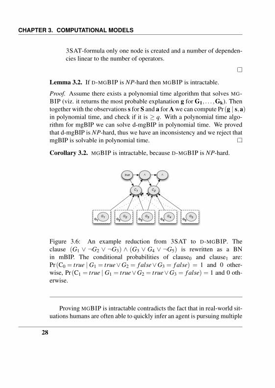
Proof. To reduce an instance of 3SAT ϕ to an instance of MGBIP B ,we create a multiple goal Gi containing one goal variable Gi for eachvariable in ϕ. For each clause in ϕ an action with the correspondingclause probability distribution is created in B and for each conjunctionin ϕ we create a conjunction node at state St+1, its conditional probabilityPr(St+1 | St ,At) = 1 if St = true and At = true and 0 otherwise. Further-more we set S0 = true in B .

We degrade excess dependencies such that if there exists a valid truthassignment for the 3SAT-formula then there exists a joint value assign-ment g for G1, . . . ,Gk for which Pr(g) ≥ q. All dependencies between agoal node and a action node for which the variable the goal node repre-

sents is not present in the clause the action node represents are degraded.Furthermore, all dependencies between At and St are degraded. Figure 3.6displays an example reduction with the degraded dependencies denoted asdotted arrows.

In B all state variables and actions variables are observed to be true andthe prior probability distribution for each goal variable is normal.

The following conditions are met, satisfying the criteria for a polyno-mial time reduction:

1. If ϕ is a yes-instance, then B is a yes-instance: For a 3SAT-formulato be satisfied, each clause must be satisfied. Per Definition 3.1 eachaction variable in B is true if and only if its corresponding clause istrue. The probability of any joint value assignment g for G1, . . . ,Gk

is 0 if it does not satisfy all clauses, or 1 if it does.

2. If B is a yes-instance, then ϕ is a yes-instance: Given the condi-tional probability Pr(St+1 | St , At), G1, . . . ,Gk need to be consis-tent with each clause variable in the BN. If B is a yes-instance thenPr(g) = 1 and the joint value assignment g for G1, . . . ,Gk is consis-tent with each clause variable. Per definition of the clause variable’sconditional probability distribution value assignment g satisfies eachclause in ϕ.

3. The reduction runs in polynomial time: For each element in the

27


3SAT-formula only one node is created and a number of dependen-cies linear to the number of operators.

Lemma 3.2. If D-MGBIP is NP-hard then MGBIP is intractable.

Proof. Assume there exists a polynomial time algorithm that solves MG-BIP (viz. it returns the most probable explanation g for G1, . . . ,Gk). Thentogether with the observations s for S and a for A we can compute Pr(g | s,a)in polynomial time, and check if it is ≥ q. With a polynomial time algo-rithm for mgBIP we can solve d-mgBIP in polynomial time. We provedthat d-mgBIP is NP-hard, thus we have an inconsistency and we reject thatmgBIP is solvable in polynomial time.

Corollary 3.2. MGBIP is intractable, because D-MGBIP is NP-hard.

true ∧

C1

∧

C2

G1G1 G2

G2 G3G3 G4

G4 G5G5

Figure 3.6: An example reduction from 3SAT to D-MGBIP. Theclause (G1 ∨ ¬G2 ∨ ¬G3) ∧ (G3 ∨ G4 ∨ ¬G5) is rewritten as a BNin mBIP. The conditional probabilities of clause0 and clause1 are:Pr(C0 = true | G1 = true∨G2 = f alse∨G3 = f alse) = 1 and 0 other-wise, Pr(C1 = true | G1 = true∨G2 = true∨G3 = f alse) = 1 and 0 oth-erwise.

Proving MGBIP is intractable contradicts the fact that in real-world sit-uations humans are often able to quickly infer an agent is pursuing multiple

28


simultaneous goals. This suggests that, if MGBIP is to be psychologicallyplausible, we need to assume that some domain-specific constraints applyin those situations that render the goal inferences tractable under the MG-BIP model (despite the model being intractable without such additionalconstraints). The next chapter describes how we set out to identify suchpossible constraints.

29

4Identifying Sources of Intractability

In order to find constraints on the input domain of MGBIP that render the(restricted) model tractable, we adopt a method for identifying sources ofintractability as described in (van Rooij, Evans, Muller, Gedge, & Ware-ham, 2008) (see also van Rooij and Wareham (2008)). The method worksas follows. One starts by identifying a set of model parameters κ in themodel M under study (for us, MGBIP), that are possible sources of in-tractability. Then one tests if it is possible to solve M in a time that cangrow excessively fast (more precisely: exponential or worse) as a functionof the elements in κ yet slowly (polynomial) in the size of the input, i.e. ifκ-M is fp-tractable.

The MGBIP model has several parameters, each of them a candidatesource of intractability. In this paper we consider five such parameters that– on intuitive grounds – may be considered candidate sources of intractabil-ity in the MGBIP model (see Table 4.2 for an overview and Fig. 4.1 for anillustration).

31

CHAPTER 4. IDENTIFYING SOURCES OF INTRACTABILITY

stomach rumbles

finds sour apple

finds candy-bar

happily eating the bar

search search eat

satisfy Hunger

good taste

big hungermedium hungerlittle hunger

yesno

T=4

k=2

g=3

G1 G2

Figure 4.1: Illustration of the Bayesian network and different parametersof the MGBIP model applied to the “mother observes son”-example.

Table 4.1: Example probability distribution over the combinations of goalvalues. In this example p = 0.6 and 1− p = 0.4.

satisfy hunger desire sweet Prbig hunger yes 0.05medium hunger yes 0.05little hunger yes 0.6big hunger no 0.3medium hunger no 0.0little hunger no 0.0

32

4.1. MGBIP FP-INTRACTABILITY

Table 4.2: A list of parameters with short descriptions and their valuesbased on the running example.

parameter description value

T maximum observations 61/T maximum observation poverty 1/6

k maximum # multiple goals 2s maximum # state values 4a maximum # action values 2g maximum # goal values 3

1− p distance from certainty 0.4

4.1 MGBIP fp-intractability

First consider parameters T , denoting the maximum number of observa-tions the observer makes, and 1/T , denoting the poverty of observations.Note that T is small if few observations are made, and 1/T is small if manyobservations are made. Based on intuition one might think, the less infor-mation we have, the harder it is to understand actions. This makes 1/T acandidate source of intractability. However as T grows, so does the size ofthe network and the necessary number of calculations and this also makesT a likely candidate source of intractability.

Second, the parameters s, a and g are the maximum number of valuesper – respectively– each state, action and goal variable. As the number ofpossible values that a variable can take increases the necessary number ofcalculations, also s, a and g is a candidate source of intractability.

Based on these parameters we prove MGBIP is fp-intractable for everysubset of parameters κ⊆ {T,1/T,g}, contradicting the intuition about theirrole in the tractability of the model. Note that based on Lemma 2.3 it isrequired to proof MGBIP intractable both for T and 1/T .

Proposition 4.1. MGBIP is not fixed-parameter tractable for {s,a,g}.

33


Proof. The NP-hardness proof of MGBIP (Section 3.3) only uses a maxi-mum of two values per variable (true or false), thus MGBIP is fp-intractableeven when the number of values per variable is small.

Proposition 4.2. MGBIP is fp-intractable for {T}.

Proof. Even when the length of the observation is 1, with any number ofmultiple goals we can encode the entire 3SAT-formula in one action vari-able and a reduction from D-3SAT to D-MGBIP would be possible. ThusMGBIP is fp-intractable even when the maximum number of available ob-servations is small.

Proposition 4.3. MGBIP is fp-intractable for {1/T}.

Proof. If the reduction from D-3SAT to D-MGBIP does not produce aninstance with a large number of states such that 1/T is small, then wecan add dummy state S

�t and action A

�t nodes. The conditional probability

Pr(S�t | St−1 = true,At−1 = true) = 1 or 0 otherwise and the conditionalprobability Pr(A�t

�� Gi = gi, . . . ,G j = g j,St−1 = true) = 1 or 0 otherwise,where gi . . .g j can be any value (i.e. A

�t is independent of all goals). This

means we can reduce any D-3SAT instance to D-MGBIP even when 1/T

is small.

Proposition 4.4. MGBIP is fp-intractable for {T,1/T}.

Proof. Assume there exists an algorithm A that solves MGBIP in polyno-mial time, given T and 1/T are constant. This means we can solve MGBIPin polynomial time, given either T or 1/T is constant. This contradictsProposition 4.2 and Proposition 4.3, thus we can conclude that such analgorithm does not exist.

Because the proofs of propositions 4.1-4.4 do not assume more thantwo values for each variable and because lemma 2.2 we observe:

Result 4.1. MGBIP is fp-intractable for every subset of parameters κ ⊆{T,1/T,g}.

34

4.2. MGBIP FP-TRACTABILITY

Result 4.1 shows – contrary to the intuitions – that none of the parametersT , 1/T and g, nor any combination of them is a source of intractabilityfor MGBIP. This means that even if we assume that one or more of theseparameters is small for the domain of application, goal inference under theMGBIP model is still intractable.

4.2 MGBIP fp-tractability

Now consider parameter k, the maximum number of multiple goals that(the observer assumes) the agent can pursue. This parameter is also anexcellent candidate source of intractability, because large k’s introduce anexponential number of combinations of possible multiple goals leading toa combinatorial explosion.

Proposition 4.5. MGBIP is fp-tractable for {k}.

Proof. We know that MPE is fixed-parameter tractable for treewidth (J.Kwisthout, 2010) and MGBIP is a special case of MPE (Section 3.3). ThusMGBIP is fixed-parameter tractable for treewidth. The treewidth of theBN underlying MGBIP grows as the number of goals increase (i.e. asthe size of the input increases). Because treewidth is the only source ofintractability for MGBIP and the number of goals is the only source thatincreases the treewidth we postulate MGBIP is fixed-parameter tractablefor the number of multiple goals.

Result 4.2. MGBIP is fp-tractable for parameter {k}.

Result 4.2 confirms parameter k is a source of intractability. This meansthat goal inference is tractable under the MGBIP model provided only thatwe impose the constraint that (the observer assumes that) the agent canpursue only a handful of goals simultaneously. Importantly, this is trueregardless the size of T , 1/T , g or 1− p. This is quite a powerful result,with great potential for explaining the speed of real-world goal inferenceswithin the confines of a BIP model. After all, it seems to be a plausibleconstraint that real-world observers can only (quickly) infer multiple goalsif agents they observe pursue only a small number of goals. This seems

35


realistic because either agents do not (typically) pursue a large number ofgoals in parallel at the same time (possibly also to keep their own planningtractable).

Finally, the parameter 1− p measures how far the most likely goal in-ference is from being completely certain (here p is the probability of themost likely explanation). If 1− p is small, this means that the most likelyexplanation is much more likely than any competitor explanation. See e.g.Table 4.1, where 1− p = 0.4 is relatively small and the most likely expla-nation satisfy hunger=little hunger, desire sweet=yes has lit-tle competition. If the value is large, it means that the most likely expla-nation has many competitor explanations of non-negligible probability. Itseems intuitive that finding the most likely explanation is easier in the for-mer case than in the latter case, and therefore also 1− p can be considereda candidate source of intractability.

Proposition 4.6. MGBIP is fp-tractable {1− p}.

Proof. It is known that MPE is fixed-parameter tractable for probabil-ity of the most probable explanation (Bodlaender, van den Eijkhof, &van der Gaag, 2002), in the sense that MPE can be solved efficiently if theprobability of the most probable explanation is high. Given that MGBIP isa special case of MPE, MGBIP is fixed-parameter tractable for probabilityof the most probable explanation.

Result 4.3. MGBIP is fp-tractable for parameter {1− p}.

Result 4.3 confirms parameter 1− p is a source of intractability. Thismeans that goal inference is tractable under the MGBIP model for thoseinputs where the most probable goal explanation is quite probable. Again,this is true regardless the size of T , 1/T , g or k. Also, this result has poten-tial for explaining the speed of real-world goal inferences within the con-fines of a BIP model, at least for certain situations—viz., those situationswhere the actions of the observed agents unambiguously suggest a partic-ular combination of goals. For all we know, real world cases of speedygoal inference may very well match exactly these situations. Whether ornot this is indeed the case is an empirical question which can be addressed

36

4.2. MGBIP FP-TRACTABILITY

by testing the speed of human goal inference for different degrees of goalambiguity.

37

5Discussion

We have analyzed the computational resource requirements of the InverseBayesian Planning (BIP) model of goal inference in order to study its vi-ability as a model of inferences made by resource-bounded minds as ourown. We generated several interesting theoretical findings. First, we ob-served that the three specialized models—M1, M2, and M3—that weredeveloped by Baker et al. (2007, 2009) to account for their experimentaldata in maze experiments are in fact computationally tractable. This meansthat these specialized Bayesian models do not seem to make unrealistic as-sumptions about the computational powers of human minds/brains, evenwhen operating on large networks of beliefs and observations. That beingsaid, these models do seem to be theoretically problematic for a differentreason: they are too specialized to count as models of goal inference ingeneral.

The over-specialization of M1, M2 and M3 is revealed when ponder-ing the assumptions that these models make about the agent and the ob-server. For instance, all three models assume that (the observer assumesthat) the agent can pursue at most one goal at a time. In the real-world,however, people often can and do act in ways so as to try and achieve two ormore goals at the same time, and observers can also often understand whatthese simultaneous goals are from observing the actors systematic behav-ior. Recall, for example, the scenario from the Introduction where the sonsearches the kitchen for a candy bar. Under different circumstances, the

39

CHAPTER 5. DISCUSSION

mother may understand that her son has even more goals at a single pointin time, for example: to still his hunger, to satisfy his craving for sweet,to see how many bars are left, to pretend that he did not hear his mom’srequest to clean up his room, to bring back a candy bar for his mom, etc.,or any combination of these goals.

To accommodate the fact that real-world goal inference is not restrictedto one goal at a time, we defined a more general BIP model – having M1,M2 and M3 as special cases – which we refer to as MULTIPLE GOALSBIP, or MGBIP for short. Complexity Analysis of the MGBIP model re-vealed that it is computationally intractable (i.e., NP-hard), meaning thatthis model, in all its generality, does indeed make unrealistic assumptionsabout the computational powers of human minds/brains. We took this neg-ative theoretical result to mean that – if the BIP model is to account forhuman goal inference at all – it must be the case that in those situationswhere humans are able to infer multiple simultaneous goals quickly andeffortlessly, specific constraints apply that render the inferences under theMGBIP model tractable.

To investigate which types of constraints could render the MGBIP modeltractable, we used a methodology for identifying sources of intractability inNP-hard computational models (see e.g. van Rooij and Wareham (2008))and derived several theoretical results. For instance, we ruled out the possi-bility of explaining speedy real-world (multiple) goal inferences by an ap-peal to small values of T (modeling situations when goals can be inferredusing only few observations) or an appeal to large values of T (modellingsituations where a lot of information is available on which to base a goalinference). Similarly, we ruled out that the speed of such inferences couldbe explained by an appeal to a small number of values per goal, action orstate node. Besides these negative theoretical results, we also had two im-portant positive results. For one, we established that as long as the numberof goals that can be simultaneously pursued, k, is not too large then goalinference is tractable under the MGBIP. Secondly we have shown that goalinference is tractable under the MGBIP model whenever the probability ofthe most likely combination of simultaneous goals, p, is not too far from 1.

Whereas our negative theoretical results are useful to clarify that tractabil-ity is not a property that is trivially achieved – and often our intuitions

40

about what constraints would render a model tractable can be wrong; cf.van Rooij et al. (2008) –, our positive results show that a model of ac-tion understanding can nevertheless be rational, Bayesian, and tractable.Moreover, the nature of the constraints that need to be introduced to renderthe Bayesian Inverse Planning model of goal inference tractable yield newempirically testable predictions.

For instance, based on our results, we predict that human participantswill be able to make quick and accurate goal inferences in the types ofexperimental set-ups such as used by Baker et al. (2007) (but see alsoCsibra, Gergely, Biro, Koos, and Brockbank (1999)), but only if the num-ber of simultaneous goals that the observed agents are pursuing is not toolarge, or the probability of the most likely combination of goals is not toosmall, or both. If both of these constraints were to be alleviated at the sametime, we would predict that human performance on the goal inference taskwould deteriorate significantly: meaning subjects will perform either slowor make bad inferences. If our prediction were to be confirmed then thiswould provide corroborative support for the BIP model of goal inference,and validate that our theoretical results help explain the tractability of hu-man goal inferences. If, on the other hand, the prediction were to be dis-confirmed, then this would suggest that either the BIP model fails as anaccount of human goal inferences, or some constraint other than the oneswe considered also suffices to render the BIP model tractable. The latteroption may then be one that BIP modelers may be interested in pursuingfurther.

In closing, we remark that our approach can be seen as exemplary ofa general strategy for dealing with intractability in any Bayesian model,whether of action understanding or otherwise. The approach reveals that– contrary to popular belief in cognitive psychology – Bayesian mod-els can possibly scale to complex, real-world domains. To achieve this,Bayesian modelers need only identify constraints that apply in the real-world and suffice to render their models’ computations tractable. By re-stricting Bayesian models in this way these models also become bettertestable: the constraints required to guarantee tractability of the modelsyield new predictions (specifically, about the speed of inferences) that canbe used to perform more stringent tests of such models.

41

6Bibliography

References

Abdelbar, A. M., & Hedetniemi, S. M. (1998). Approximating MAPsfor belief networks is NP-hard and other theorems. Artificial Intelli-

gence, 102, 21–38.Baker, C. L., Saxe, R., & Tenenbaum, J. B. (2009). Action understanding

as inverse planning. Cognition(113), 329–349.Baker, C. L., Tenenbaum, J., & Saxe, R. (2007, Jan). Goal inference as

inverse planning. Proceedings of the 29th meeting of the Cognitive

Science Society.Baldwin, D. A., & Baird, J. A. (2001). Discerning intentions in dynamic

human action. Trends in Cognitive Sciences, 5(4), 171–178.Bodlaender, H. L., van den Eijkhof, F., & van der Gaag, L. C. (2002).

On the complexity of the MPA problem in probabilistic networks.In F. van Harmelen (Ed.), Proceedings 15th european conference on

artificial intelligence (pp. 675–679). Amsterdam, the Netherlands:IOS Press.

Charniak, E., & Shimony, S. E. (1990). Probabilistic semantics for costbased abduction. In Aaai (p. 106-111).

Chater, N., Tenenbaum, J. B., & Yuille, A. (2006). Probabilistic modelsof cognition: Conceptual foundations. Trends in Cognitive Sciences,10(7), 287 - 291. (Special issue: Probabilistic models of cognition)

43

CHAPTER 6. BIBLIOGRAPHY

Csibra, G., Gergely, G., Biro, S., Koos, O., & Brockbank, M. (1999). Goalattribution without agency cues: the perception of ’pure reason’ ininfancy. Cognition, 72, 237–267.

Cuijpers, R. H., Schie, H. T. van, Koppen, M., Erlhagen, W., & Bekkering,H. (2006, Jan). Goals and means in action observation: A computa-tional approach. Neural Networks.

Downey, R., & Fellows, M. (1998). Parameterized complexity (Heidelberg,Ed.). Springer-Verlag.

Garey, M. R., & Johnson, D. S. (1979). Computers and intractability: A

guide to the theory of np-completeness (series of books in the math-

ematical sciences). W. H. Freeman.Gergely, G., Nadasdy, Z., Csibra, G., & Biro, S. (1995). Taking the inten-

tional stance at 12 months of age. Cognition, 56, 165–193.Ghahramani, Z. (1998). Learning dynamic Bayesian networks. In Adap-

tive processing of sequences and data structures (pp. 168–197).Springer-Verlag.

Gigerenzer, G., Hoffrage, U., & Goldstein, D. G. (2008). Fast and frugalheuristics are plausible models of congition: Reply to Dougherty,Franco-Watkins, and Thomas (2008). Psychological Review, 115,230–239.

Hassin, R., Aarts, H., & Ferguson, M. (2005, Jan). Automatic goal infer-ences. Journal of Experimental Social Psychology.

Jensen, F. V., & Nielsen, T. D. (2007). Bayesian networks and decision

graphs (Second ed.). New York: Springer Verlag.Kiraly, I., Jovanovic, B., & Prinz, W. (2003, Jan). The early origins of goal

attribution in infancy. Consciousness and Cognition.Kwisthout, J. (2010). Most probable explanations in bayesian networks:

complexity and algorithms.

Kwisthout, J. H. P. (2009). The computational complexity of probabilis-

tic networks. Unpublished doctoral dissertation, Faculty of Science,Utrecht University, The Netherlands.

Marr, D. (1982). Vision : a computational investigation into the human

representation and processing of visual information / david marr

[Book]. W.H. Freeman, San Francisco ; New York :.

44

References

Pearl, J. (1988). Probabilistic reasoning in intelligent systems: Networks

of plausible inference. Morgan Kaufmann, Palo Alto.Robertson, N., & Seymour, P. (1986). Graph minors II: Algorithmic as-

pects of tree-width. Journal of Algorithms, 7, 309–322.Schultz, R. T., Grelotti, D. J., Klink, A., Kleinman, J., Gaag, C. van der,

& Marois, R. (2003). The role of the fusiform face area in socialcognition: Implications for the pathobiology of autism. Philosoph-

ical Transactions of Royal Society of London, Series B: Biological

Scences(358(1430)), 415–427.Seroussi, B., & Golmard, J. (1994, Jan). An algorithm directly finding the

k-most probable configurations in bayesian networks. International

Journal of Approximate Reasoning, 11(3), 205–233.Sipser, M. (1992). The history and status of the p versus np question. In

Stoc ’92: Proceedings of the twenty-fourth annual acm symposium

on theory of computing (pp. 603–618). New York, NY, USA: ACM.Sy, B. K. (1992). Reasoning MPE to multiply connected belief networks

using message-passing. In Proceedings of the tenth national confer-

ence on artificial intelligence (pp. 570–576).Ullman, T. D., Baker, C. L., Macindoe, O., Goodman, O. E. N. D., &

Tenenbaum, J. B. (2009). Help or hinder: Bayesian models of socialgoal inference. NIPS.

van Rooij, I., Evans, P., Muller, M., Gedge, J., & Wareham, T. (2008).Identifying sources of intractability in cognitive models: An illus-tration using analogical structure mapping. In K. M. B. C Love &V. M. S. (Eds.) (Eds.), Proceedings of the 30th annual conference of

the cognitive science society (pp. 915–920). Austin, TX: CognitiveScience Society.

van Rooij, I., & Wareham, T. (2008). Parameterized complexity in cog-nitive modeling: Foundations, applications and opportunities. Com-

puter Journal, 51(3), 385–404.

45

how action understanding can be rational, bayesian … · 2010-09-20 · universe and ﬁnding the...

Documents