housing construction cycles and interest rates · conference and at an internal reserve bank...
TRANSCRIPT

HOUSING CONSTRUCTION CYCLES ANDINTEREST RATES
Laura Berger-Thomson and Luci Ellis
Research Discussion Paper2004-08
October 2004
Economic GroupReserve Bank of Australia
The authors are grateful to participants at the 2004 Econometric SocietyConference and at an internal Reserve Bank seminar for their helpful comments.Responsibility for any remaining errors rests with the authors. The viewsexpressed in this paper are those of the authors and should not be attributed tothe Reserve Bank.

Abstract
Housing investment is one of the most cyclical components of GDP. Much of thatcyclicality stems from the sector’s sensitivity to interest rates, but it is also possiblethat construction lags generate intrinsic cyclicality in this sector. Although thehousing sector is generally considered to be more interest-sensitive than theeconomy as a whole, the degree of this sensitivity seems to vary between countriesand through time. In this paper, we model the housing markets in Australia, theUnited States, the United Kingdom and Canada using a structural three-stage least-squares system. We document the variations in the housing sector’s cyclicality andsensitivity to movements in interest rates, and attempt to determine the underlyingcauses of these differences.
JEL Classification Numbers: E22, E32, R21, R31Keywords: cycles, housing construction, interest rates
i

Table of Contents
1. Introduction 1
2. Housing Investment Cycles in Developed Countries 3
3. Models of Housing Demand and Supply 7
3.1 Theories of Housing Demand 8
3.2 Modelling Housing Demand 9
3.3 Housing Supply 11
4. Empirical Estimates 12
4.1 Data 13
4.2 Preferred Specification 14
4.3 Results 16
5. Discussion of Results 23
6. Conclusion 29
Appendix A: Data Sources 31
Appendix B: Econometric Results 33
References 38
ii

HOUSING CONSTRUCTION CYCLES ANDINTEREST RATES
Laura Berger-Thomson and Luci Ellis
1. Introduction
Housing investment is one of the most cyclical components of output in manyindustrialised economies, and likewise one of the more interest-sensitive. Itis likely that much of the cyclicality derives from the interest sensitivity, butconstruction lags and resultant sluggish supply might also lead to intrinsicallycyclical responses of output to demand shocks. The particular interest sensitivityof housing demand seems to stem partly from frictions in capital markets. Sincethese can change over time, it is also likely that the interest sensitivity andcyclicality of housing construction can vary through time and across countries.
In this paper, we use econometric techniques to discern whether the observedcyclicality is intrinsic to the construction sector, or a consequence of its interestsensitivity, and to document differences in this interest sensitivity across fourEnglish-speaking countries. In doing so, we are effectively doing for quantitieswhat Sutton (2002) did for prices. We then attempt to reconcile these differencesbased on institutional differences in the housing construction and mortgage financemarkets. The goals of the paper are thus similar to those of Aoki, Proudmanand Vlieghe (2002) and McCarthy and Peach (2002), who identified changes inthe policy transmission mechanism in the United Kingdom and United Statesassociated with financial sector deregulation.
Our focus on institutional factors places this paper within a substantial recentliterature on the different macroeconomic effects of housing market developments,particularly in the context of European Monetary Union (Maclennan, Muellbauerand Stephens 1998; Tsatsaronis and Zhu 2004, for example). Our paper extendsthe analysis in that literature by proposing a new approach to structural modellingof the sector. This allows us to disentangle supply-side from demand-side factors,and in particular, establish the relative importance ofintrinsic cyclicality causedby sluggish supply, andextrinsiccyclicality resulting from demand responses tothe interest-rate cycle.

2
We find a dominant role forextrinsic interest-rate cyclicality in explaining thehousing cycle. However, there is also some weak evidence ofintrinsic cyclicalityin some of the countries studied, driven by the interaction between sluggish supplyand flexible demand. When a demand shock occurs, supply adjusts only gradually,thereby generating a hog-cycle type effect on both prices and quantities supplied.This is partly due to the fact that the change in the housing stock that householdsdemand can be much larger than the feasible flow of new housing supplied inany one period, and partly due to time-to-build constraints on the construction ofthat new supply. The extent of the sluggishness in supply presumably dependson a range of factors, including the structure of the construction industry,land availability, regulatory policies and other country-specific factors. It is notfeasible to reconcile all these supply-side differences with the quantitative cross-country differences in our estimated supply functions. However, they clearly haveconsiderable scope to affect the magnitude of the transmission of movements ininterest rates to housing construction.
When comparing the results across countries, we find evidence of significantdifferences in the (extrinsic) cyclicality of housing investment, even after allowingfor the different paths of interest rates experienced in different countries. That is,our structural modelling appears to identify cross-country differences in the directresponse of housing demand to movements in interest rates. This is compoundedby variations in the income sensitivity of housing demand across countries.Although we do not formally model the response of permanent income to interestrates, it appears that the direct interest-rate effect and the indirect effect via incomerepresent two channels of the transmission mechanism from monetary policy todemand for new and improved housing.
Institutional arrangements in mortgage finance markets clearly matter indetermining these different degrees of interest sensitivity and income sensitivity.Although financial deregulation did not appear to alter demand behaviour inAustralia, our results confirm McCarthy and Peach’s (2002) earlier findings of astructural change in the dynamic behaviour of housing demand following financialmarket deregulation in the United States. As well as explaining structural breaks inhousing market behaviour within a country, institutional factors might help explainthe cross-country differences identified in our empirical results. The prevalence offixed-rate versus variable-rate mortgage finance appears particularly important,which in turn depends on a range of taxation, regulatory and other policies.

3
2. Housing Investment Cycles in Developed Countries
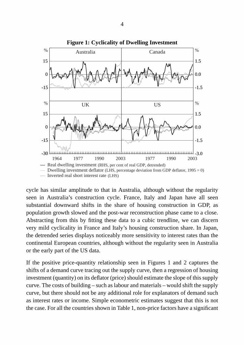
The key facts we seek to explain are shown in Figures 1 and 2. Housingconstruction as a share of GDP has a negative relationship with interest rates.1
Construction prices are positively associated with construction activity, althoughthere is a slight lag between the movement in activity and the change in prices.This lines up with the observations of Topel and Rosen (1988) for earlier US data,that the price-volume relationship is mainly due to shifts in the demand for newhousing tracing out a largely unchanged supply curve. In this context, interest ratesappear to serve as a demand shifter. A similar picture applies if growth rates areused rather than shares of GDP, or if housing starts are used instead of nationalaccounts measures.
Within these relationships, however, there are clear differences both betweencountries and across time; these differences are the focus of this paper. Inparticular, the regularity of the housing cycle in Australia in recent decades isnot matched by any of the other countries shown here. The early part of the USdata is very cyclical, but as noted by McCarthy and Peach (2002), this pattern hasbeen more muted since the early 1980s. However, this change cannot be whollyattributed to the milder cycle in interest rates more recently.
Although the share of nominal housing construction in nominal GDP for the UKdisplays some cyclicality, in volume terms the share has been virtually flat formore than a decade. There was a clear cycle in construction in the late 1980s, butthis was almost certainly the result of the housing boom occurring at that time,mainly due to factors other than monetary policy and interest rates (Attanasio andWeber 1994; Ortalo-Magne and Rady 1999). The interest sensitivity of the UKhousing sector seems to manifest primarily in structure prices, and in the landprices implied by the total price of existing housing.
In New Zealand and Canada, the housing construction share is more variable overtime than in the UK or recent US data. It appears that the housing construction
1 Terminology in national data sources can differ substantially. To maintain a consistent setof terminology in this paper, we refer to the dwelling investment component of the nationalaccounts as ‘housing construction’ or ‘dwelling investment’, its associated price deflator as‘structure prices’, and building commencements as ‘housing starts’. ‘House prices’ denotes theprices including land or location value actually paid by home owners. Figures 1 and 2 show theshare of housing construction in GDP detrended using a simple cubic time trend.
4
Figure 1: Cyclicality of Dwelling Investment
Australia
-3.0
-1.5
0.0
1.5
-3.0
-1.5
0.0
1.5
-30
-15
0
15
-30
-15
0
15
-15
0
15
-15
0
15
-1.5
0.0
1.5
-1.5
0.0
1.5
Canada
(LHS)
–– Real dwelling investment–– Dwelling investment deflator–– Inverted real short interest rate
(RHS, per cent of real GDP, detrended)(LHS, percentage deviation from GDP deflator, 1995 = 0)
2003199019772003199019771964
UK US
%
%
%
%
cycle has similar amplitude to that in Australia, although without the regularityseen in Australia’s construction cycle. France, Italy and Japan have all seensubstantial downward shifts in the share of housing construction in GDP, aspopulation growth slowed and the post-war reconstruction phase came to a close.Abstracting from this by fitting these data to a cubic trendline, we can discernvery mild cyclicality in France and Italy’s housing construction share. In Japan,the detrended series displays noticeably more sensitivity to interest rates than thecontinental European countries, although without the regularity seen in Australiaor the early part of the US data.
If the positive price-quantity relationship seen in Figures 1 and 2 captures theshifts of a demand curve tracing out the supply curve, then a regression of housinginvestment (quantity) on its deflator (price) should estimate the slope of this supplycurve. The costs of building – such as labour and materials – would shift the supplycurve, but there should not be any additional role for explanators of demand suchas interest rates or income. Simple econometric estimates suggest that this is notthe case. For all the countries shown in Table 1, non-price factors have a significant

5
Figure 2: Cyclicality of Dwelling Investment
200319922003
Italy
-2
-1
0
1
-2
-1
0
1
-30
-15
0
15
-30
-15
0
15
-30
0
30
-30
0
30
-0.4
0.0
0.4
-0.4
0.0
0.4
France
New ZealandJapan
% %
% %
198119921970 1981
(LHS)
–– Real dwelling investment–– Dwelling investment deflator–– Inverted real short interest rate
(RHS, per cent of real GDP, detrended)(LHS, percentage deviation from GDP deflator, 1995 = 0)
relationship with housing construction (and housing starts), even after controllingfor structure prices in the form of the housing construction deflator. This isconsistent with similar results cited in Egebo, Richardson and Lienert (1990).Reduced-form VARs constructed along the lines of those in Aokiet al (2002) andMcCarthy and Peach (2002) were also consistent with this finding; these resultsare available from the authors.
In particular, the estimated coefficients on interest rates are negative, andsignificant for all countries shown except the United Kingdom and Japan. Part ofthe reason for this could be that interest rates are also a supply shifter, so that thereduced-form estimates are not tracing out an unchanged supply curve. Financingcosts are one of the costs of constructing housing, so an increase in interest rateswould shift the supply curve left, and reduce quantity supplied. The conclusionof earlier work, however, is that the extent of the estimated relationship betweeninterest rates and construction is too great to be reconciled with financing costsover the duration of a construction project (Topel and Rosen 1988).

6
Table 1: Coefficient Signs in Reduced-form Models of Dwelling InvestmentSimple model Expanded model
Constructioncosts
Structureprices
Constructioncosts
Structureprices
Interest rates Income
Australia [+] − [+] [−] [−] +Canada [+] − − − − +France [−] [+] [+] [+] [−] [−]
Japan [+] [−] + [−] − +Netherlands [+] [−] [+] + [−] [−]
UK [−] − + + [−] [−]
US − [+] [+] [+] [−] [−]
Notes: Plus and minus symbols indicate sign of estimated coefficient. Square brackets indicate that the estimatedcoefficient is significant at the 10 per cent level. Up to four lags of the dependent variable were also includedin both equations.
One initially plausible explanation for housing investment’s interest sensitivity– even after controlling for prices – is that suppliers and demanders of housingare not paying the same price. Builders are affected by the cost and sale priceof the structure. Home buyers, by contrast, pay the total price of the dwelling,including the cost of the land. As can be seen in Figure 3, the implied priceof residential land generally swings around more than the price of the structure,driving significant, usually pro-cyclical, wedges between supply price and demandprice. However, many of the causes of this wedge between the two prices, suchas zoning laws (Glaeser and Gyourko 2002) and land shortages (Kenny 1999),do not appear to be the main driver of housing cycles. Chinloy (1996) foundthat cycles in housing construction can exist even when there is plenty of landfor development and few zoning restrictions or rent controls to distort the supplydecision. In English-speaking countries at least, the greater correlation of interestrates with total housing prices than with structure prices suggests that rates explainmuch of this pro-cyclical wedge.
Despite the apparent positive relationship between prices and construction visiblein Figures 1 and 2, the results in Table 1 force us to conclude that this relationshipis not capturing a stable supply function. This implies that a reduced-formestimation strategy is not appropriate. To understand the causes of interest-rate sensitivity in housing construction, we must turn instead to more structuralmodelling, and try to disentangle demand-side from supply-side influences. In thenext section, we develop some variations on existing theoretical models of housing

7
Figure 3: Cyclicality of House and Structure PricesYear-ended percentage change
Australia
-20
0
20
40
-20
0
20
40
-20
0
20
40
-20
0
20
40
0
20
40
0
20
40
0
20
40
0
20
40
Canada
2003199019772003199019771964
UK US
%
%
%
%
House prices
Structureprices
(including land)
demand and supply, which we then translate into empirical models to be estimatedin Section 4.
3. Models of Housing Demand and Supply
In this section, we develop models for supply and demand for both the number ofdwellings and the total value of housing construction. This distinction is necessarybecause, unlike many other goods, production represents an incremental additionto a stock of housing, while demand for housing can be either for the asset, or forthe implied flow of services derived from living in a dwelling. In line with previousmacroeconomic models of housing construction, we treat the housing market as anational market, even though supply of a new dwelling in one city will not satisfyexcess demand in another.

8
3.1 Theories of Housing Demand
The standard analysis of housing demand recognises that a dwelling is both aprovider of a flow of housing services and an asset (Henderson and Ioannides1986; Ioannides and Rosenthal 1994). Assuming housing services are a normalgood,flow demand is decreasing in its relative price and increasing in householdincome. This flow demand is then converted into a desired stock of housing,usually – but not always (e.g., Henderson and Ioannides 1983) – by assumingthat services vary proportionately with the stock.
The price of housing services differs from the purchase price: for households thatrent, it is simply the rent paid. Households that own their own home incur animputed user cost, for example as shown in Equation (1). This includes the costsof maintenance and depreciation(δ ), plus the opportunity cost of not investing insome other asset with a nominal return ofi, partly offset by the expected rate ofcapital gain or loss on housingHe. H is the price per (quality-adjusted) unit ofhousing.2 Because there are differences between both the kinds of households thatown versus those that rent, and between the kinds of housing they occupy, this usercost is unlikely to arbitrage to measured rents (Ioannides and Rosenthal 1994).
User cost= (i +δ −π− He)×H (1)
Assetdemand for housing is demand for a stock. Housing can return a flow ofactual or imputed rental incomeRh, and a capital gain. In the absence of capital-market imperfections or financial regulation, the total (risk-adjusted) return onhousing assets should arbitrage to that on other assets, proxied by a real post-taxinterest rate in Equation (2) (Meen 1990).
Rh+ H−δ = (1− τ)i(t)−π(t) (2)
When households’ consumption and asset demands differ, as is possible giventhe differences between Equations (1) and (2), the discrepancy is resolved bytheir tenure decision. If the stock equivalent of consumption demand exceeds
2 If interest payments on mortgage debt are tax-deductible, then the after-tax nominal interestrate (1− τ)i replaces the pre-tax rate presented here (Meen 1990, 2000). In Australia,mortgage interest is not deductible; see Bourassa and Hendershott (1992) for discussion ofthe implications of this. Equation (2) ignores any differences between the capital gains taxtreatment of owner-occupied versus investor housing, or across countries.

9
investment demand, the household rents, while if the reverse is true, it owns its ownhome and possibly also some investment properties. Some households might alsoown even if their consumption demand exceeds their unconstrained asset demand.Henderson and Ioannides (1983) argue that an externality exists favouring owner-occupation, because landlords cannot completely extract from tenants the costsof the wear and tear they impose on their home. This externality forces the twodemands together. This suggests one reason why housing demand behaviour mightvary across countries. If the laws relating to landlord-tenant relations differ, somight the extent of this externality and thus of any deviation between actualdemand and predicted consumption demand for housing.
Increases in real interest rates reduce consumption demand for housingthrough intertemporal substitution and investment demand because the return onalternative assets rises. Distortions in the housing finance market can generateother channels through which interest rates affect demand, in ways that mightdiffer across countries. For example, nominal interest rates can affect housingdemand if credit constraints limit the size of the mortgage repayment relative toincome (Lessard and Modigliani 1975; Stevens 1997). Downpayment constraints(Stein 1995) and restrictions on the supply of credit (Throop 1986; McCarthy andPeach 2002) might also influence the interest sensitivity of housing demand.
3.2 Modelling Housing Demand
To translate these theoretical models of individual household behaviour intoempirical estimates, previous work has generally assumed that the housing stockis fixed in the short run, and placed housing prices on the left-hand side of theequation (Meen 1990). In this paper, we augment that approach by treating theamount of housing demanded by one household separately from the number ofdwellings being demanded.
In the long run, the number of new dwellings demanded is proportional to thenumber of households, assuming a constant vacancy rate. In the short run, therate of household formation can vary in response to macroeconomic factorssuch as income (Y), (total) housing prices (Pn), structure prices (Ps) and interestrates (i). The stock of dwellings can also move differently from the number ofhouseholds, resulting in fluctuations in the vacancy rate (vac), calculated as thedifference between the (log) housing stock and the (log) number of households.

10
This naturally leads to an error-correction form for the demand for the (net)number of new dwellings (q in logs), as shown in Equation (3) with lower-caseletters denoting log levels except for interest rates.
∆qt =α0−α1(qt−1+α2vact−1+α3hhgrowtht−1)+∑
i
α4i ∆qt−i
+∑
i
α5i ∆ph,t−i +∑
i
α6i ∆yt−i +∑
i
α7i it−i +∑
i
α8i ∆ps,t−i
(3)
The log change in the number of dwellings represents completions of newdwellings and conversions, less demolitions. However because of data limitations,our empirical models use housing starts instead, which will affect the estimateddynamics’ lag structure.
Given this specification for quantity orflow demand for new dwellings, anequation for house prices can be motivated as capturing the demand for the qualityof the housingstockby the representative household. Previous work has not beensupportive of a long-run cointegrating relationship between housing prices andfundamentals such as income (Gallin 2003). In contrast, we were able to find asignificant long-run relationship between housing prices and a measure of incomefor Australia and the US, but not the UK or Canada. Where such a relationshipcould not be found, we assumed instead that the relative price of housing – thedifference between the log price of housingph and the log general price levelp– is constant in the long run.3 Short-run fluctuations in house prices may then bedriven by fluctuations in income, the prices of a house including land (ph) and ofimproved housing quality (structure pricesps) and the price of finance (interestrates), as shown in Equation (4), while the scarcity of housing (the vacancy rate)matters at longer horizons.
∆ph,t =β0−β1(ph,t−1− pt−1−β2yt−1+β3vact−1)+∑
j
β4 j∆ps,t− j
+∑
j
β5 j∆ph,t− j +∑
i
β6 j∆yt− j +∑
j
β7 j it− j
(4)
In principle, both real and nominal interest rates should enter into the estimation;real rates enter into underlying arbitrage conditions, but nominal rates capture the
3 We impose this restriction by assuming the long-run coefficient on the general price level isequal to that on housing prices, but with the opposite sign. The data do not reject this restriction.
11
effects of some credit market imperfections. Alternatively, nominal interest ratesand inflation could be included, and the difference between the absolute valuesof the resulting estimated coefficients attributed to the effect of nominal ratesindependent of that of real rates.4 We use policy interest rates in all our modelsfor cross-country comparability, even though this is not the mortgage rate thathouseholds actually pay.
3.3 Housing Supply
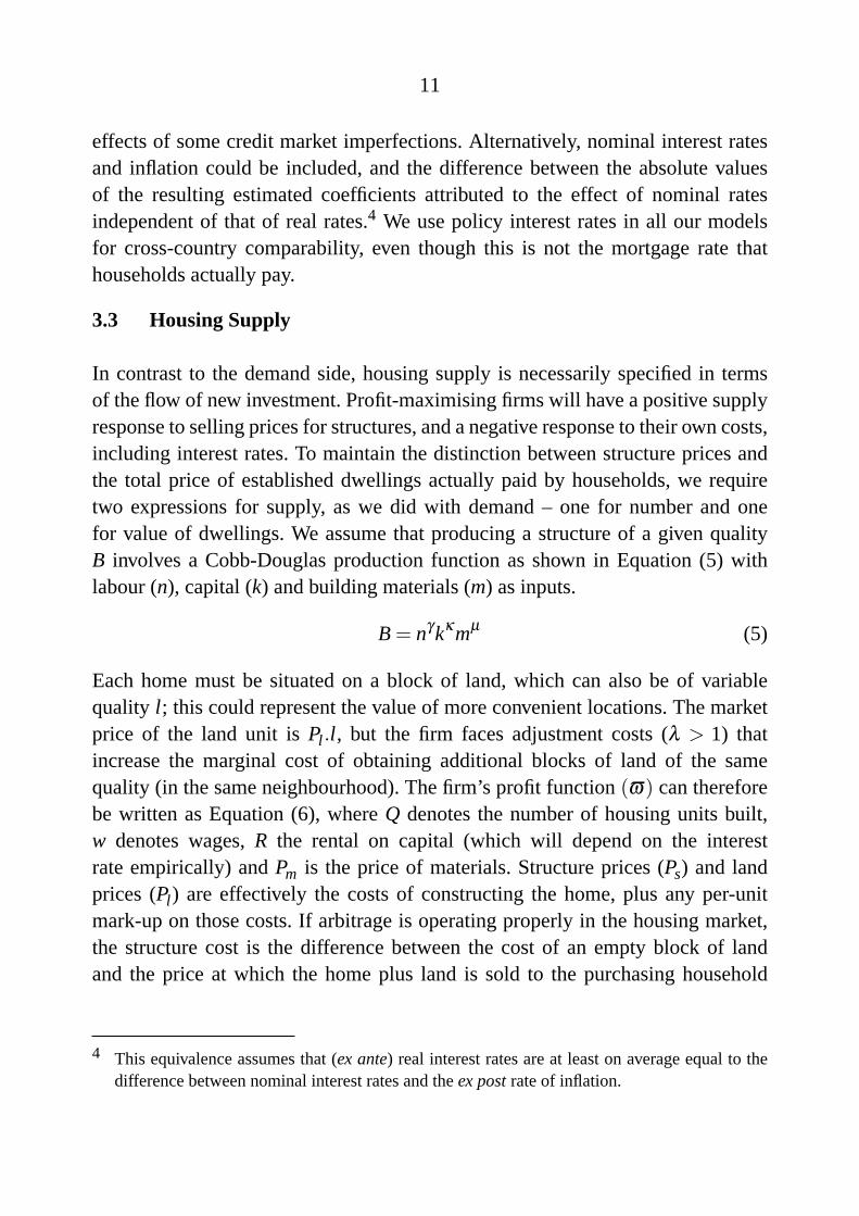
In contrast to the demand side, housing supply is necessarily specified in termsof the flow of new investment. Profit-maximising firms will have a positive supplyresponse to selling prices for structures, and a negative response to their own costs,including interest rates. To maintain the distinction between structure prices andthe total price of established dwellings actually paid by households, we requiretwo expressions for supply, as we did with demand – one for number and onefor value of dwellings. We assume that producing a structure of a given qualityB involves a Cobb-Douglas production function as shown in Equation (5) withlabour (n), capital (k) and building materials (m) as inputs.
B = nγkκmµ (5)
Each home must be situated on a block of land, which can also be of variablequality l ; this could represent the value of more convenient locations. The marketprice of the land unit isPl .l , but the firm faces adjustment costs (λ > 1) thatincrease the marginal cost of obtaining additional blocks of land of the samequality (in the same neighbourhood). The firm’s profit function(ϖ) can thereforebe written as Equation (6), whereQ denotes the number of housing units built,w denotes wages,R the rental on capital (which will depend on the interestrate empirically) andPm is the price of materials. Structure prices (Ps) and landprices (Pl ) are effectively the costs of constructing the home, plus any per-unitmark-up on those costs. If arbitrage is operating properly in the housing market,the structure cost is the difference between the cost of an empty block of landand the price at which the home plus land is sold to the purchasing household
4 This equivalence assumes that (ex ante) real interest rates are at least on average equal to thedifference between nominal interest rates and theex postrate of inflation.
12
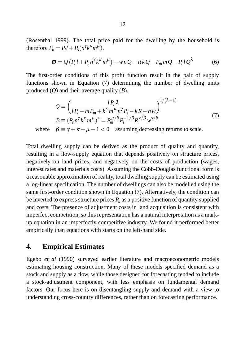
(Rosenthal 1999). The total price paid for the dwelling by the household isthereforePh = Pl l +Ps(n
γkκmµ).
ϖ = Q(Pl l +Psnγ kκ mµ
)−wnQ−RkQ−PmmQ−Pl l Q
λ (6)
The first-order conditions of this profit function result in the pair of supplyfunctions shown in Equation (7) determining the number of dwelling unitsproduced (Q) and their average quality (B).
Q =(
l Pl λ
l Pl −mPm+kκ mµ nγ Ps−kR−nw
)1/(λ−1)
B≡ (Psnγ kκ mµ)∗ = Pµ/β
m P−1/β
s Rκ/β wγ/β
where β ≡ γ +κ + µ−1 < 0 assuming decreasing returns to scale.
(7)
Total dwelling supply can be derived as the product of quality and quantity,resulting in a flow-supply equation that depends positively on structure prices,negatively on land prices, and negatively on the costs of production (wages,interest rates and materials costs). Assuming the Cobb-Douglas functional form isa reasonable approximation of reality, total dwelling supply can be estimated usinga log-linear specification. The number of dwellings can also be modelled using thesame first-order condition shown in Equation (7). Alternatively, the condition canbe inverted to express structure pricesPs as a positive function of quantity suppliedand costs. The presence of adjustment costs in land acquisition is consistent withimperfect competition, so this representation has a natural interpretation as a mark-up equation in an imperfectly competitive industry. We found it performed betterempirically than equations with starts on the left-hand side.
4. Empirical Estimates
Egebo et al (1990) surveyed earlier literature and macroeconometric modelsestimating housing construction. Many of these models specified demand as astock and supply as a flow, while those designed for forecasting tended to includea stock-adjustment component, with less emphasis on fundamental demandfactors. Our focus here is on disentangling supply and demand with a view tounderstanding cross-country differences, rather than on forecasting performance.

13
4.1 Data
Limitations on data availability confine our econometric modelling to fourcountries – Australia, Canada, the United States and the United Kingdom. Themodels of demand and supply developed in the previous section involve twomeasures of quantity – number and total investment (number times quality) – andtwo prices: the structure price and the total price including land. For quantities,we use housing starts from building activity surveys and housing constructioninvestment from the national accounts. The deflator for housing construction isused as the measure of structure prices. Total housing prices are represented asmedian sale prices of established dwellings; these can be obtained from lenders,real estate associations or statistical agencies, depending on the country. Thestructure price measure captures the cost of a constant volume of construction,but the average or median house price does not generally incorporate an effectivequality adjustment. Thus there might be a wedge between these two pricemeasures beyond that caused by land prices, which would introduce a distortioninto our econometric results.
Permanent income is proxied by the sum of non-durables and servicesconsumption, except for the UK, where total consumption is used. We usedmaterials and labour costs series specific to the construction industry to captureconstruction costs, except for Canada where only economy-wide materials priceindices were available. We use the policy interest rate, not the mortgage rate, toensure that we are comparing the effects of the same kinds of shocks to interestrates across countries. This may reduce the models’ fit if mortgage rates key offlong rates as in the US, or if interest margins have varied over time, as in Australia.On the other hand, it means we do not need to model pass-through of policy ratesto mortgage rates separately.
As shown in Equation (3), our preferred theoretical model of demand for thenumber of dwellings is driven by the number of households in the long run. Ourquarterly series for the UK, the US and Canada are interpolations of annual data,while for Australia, we estimate the number of households using an estimatedhousehold formation rate and population data. These smoothed data series avoidthe effects of short-run endogeneity in the household formation decision.

14
Demand for and supply of public housing presumably respond to different forcesthan the market-oriented forces considered here. However, public housing clearlysatisfies the flow (consumption) demand of some households. If the share ofpublic housing changes over time, as has been true in the UK (Attanasio andWeber 1994), time-series estimates for demand for privately owned housing wouldbe distorted by the exclusion of public housing. Thus it would be preferable toconsider all dwellings in our estimates, accounting for the differing influences ofthe public and private sectors. However, because of data constraints in the otherthree countries, we are only able to include public dwelling construction in theUK, though it is arguably most important there. Further details on the data arecontained in Appendix A.
4.2 Preferred Specification
We have four endogenous variables – two different prices, plus quantity andquality of new housing – and four equations determining them in the formof supply and demand equations for both quantity and quality. Many of theexplanators are clearly endogenous and likely to be correlated with the equations’error terms.5 The error terms are likely to be correlated across equations as well,given the tight relationship between variables such as housing starts (quantity)and dwelling investment (quantity multiplied by quality). Therefore we usedthe three-stage least squares instrumental variables estimator to avoid statisticalproblems involved with using endogenous explanators. All current-dated variablesare treated as potentially endogenous, while all lag-dated variables are takento be potential instruments. We followed a general-to-specific methodology toarrive at a preferred dynamic specification, but by default we retained variablesas instruments that had been dropped from the second-stage estimates of thebehavioural equations. This helped avoid serial correlation in the residuals, whichwould have resulted in inconsistent parameter estimates. Serial correlation wouldhave been especially problematic in an instrumental variables estimate, becausethe lagged variables used as instruments would also be correlated with the errors.
5 A version of the model including an equation for construction costs in the model did notmaterially change the results.

15
To obtain sensible results, we also made several modifications to the specificationsset out in Section 3. As highlighted earlier, we imposed the restriction, inEquation (4) for house prices, that the coefficients on the lagged house priceand the general price level be of equal and opposite sign. In the short-rundynamics, we allowed some departure from this by including house price inflationand CPI inflation separately. For Canada and the UK, therelative price ofhousing is the only long-run determinant of house prices. For Australia, theaggregate level of income is also important in the long run, while in the US,average household income matters.6 Similarly, we allowed for incomplete short-run arbitrage between house-and-land packages and empty blocks of land byincluding the total price of housing in the structure price equation. This was animportant modification; it seems that builders/developers do have scope to settotal prices, as in all cases structure prices depend positively on house (and thusimplicitly land) prices.
Following Tsatsaronis and Zhu (2004), we also allowed for mortgage tilt and otherfinancial frictions to affect housing demand by including nominal interest ratesas an explanator. Because the inflation rate is already in the short-run dynamicsto capture the effects of relative housing prices discussed above, including bothnominal and real interest rates directly would introduce excessive collinearity.Therefore we included nominal rates on their own and allowed the coefficienton inflation to mop up both the effect of real interest rates and of relative houseprice inflation. The risk in this approach is that the coefficient on inflation mightalso be picking up trends that the cointegrating relationships are not adequatelycapturing; in some cases these were quite imprecisely estimated. Nominal interestrates fell substantially in the countries studied, in line with the disinflations of the1980s and early 1990s.
Finally, we allowed for structural change, mainly in the short-run dynamics of themodels, to capture the effects of financial deregulation, and of the introduction ofGoods and Services Taxes (GST) in Australia and Canada. In line with the resultsin Aoki et al(2002) and McCarthy and Peach (2002), we find significant structuralinstability in the United States and the United Kingdom. In both countries, Chowtests suggest there is a break around the beginning of 1986, consistent with the
6 This specification of income was extended to the short-run dynamic terms for consistency.

16
timing of financial deregulation.7 Although there was some weak evidence ofstructural instability in the Australian model, we found that the model fit the databetter without it. There was no evidence of structural instability in the model forCanada. This is consistent with the lack of a clear episode of financial deregulationin the sample period, since the mortgage market in Canada was already quitelightly regulated as early as the 1960s (Edey and Hviding 1995).
The introduction of a GST permanently shifts the level of structure prices. This iscaptured as a permanent shift dummy in the post-introduction period, although theeffect was not significant for Canada. We also included a dummy in the quarter ofintroduction to account for the one-off increase in the growth rate of prices. Priceswere higher and production lower after the GST’s introduction in both countries.We also found evidence of a significant ‘bring-forward’ effect in Australia –but not Canada – in the quarters immediately preceding the GST’s introduction.Demand was temporarily higher as households brought their construction plansahead of the GST’s start date. Supply was also temporarily higher to takeadvantage of this temporary surge in demand; for example, construction firmswere observed to be working unusually high levels of overtime in the period priorto the GST’s introduction in Australia.
4.3 Results
The models presented in Appendix B match the data reasonably well, but plotsindicate that the fitted values for housing construction tend to undershoot theactual series for Australia, Canada and the UK in the last couple of years in thesample (Figure 4). It seems likely that some other omitted factor affected outcomesover this period; it may be that households have been spending on housingout of transitory as well as permanent income. Another possibility is that thedifferent treatment of changes in average housing quality in the two price series ishampering separate identification of supply and demand. In any case, the (demand)equation for house prices is not particularly precisely estimated for any of thecountries, although in this respect our results compare fairly well with previous
7 Although statistical tests exist for dating structural breaks in multivariate data (Andrews 1993;Bai, Lumsdaine and Stock 1998), we are not aware of any work on the properties of these testsin an instrumental variables framework.

17
literature. Some models of housing prices alone (Bourassa and Hendershott 1995;Abraham and Hendershott 1996, for example) incorporate ‘bubble’ components,implying extrapolative expectations, to account for movements in housing pricesthat cannot be explained by macroeconomic fundamentals. It may be that ourmodels are not properly capturing such a phenomenon, even though the equationsfor housing prices already include lagged price growth terms as explanators.
Figure 4: Dwelling InvestmentPer cent of GDP
Australia
Modelled
US
Actual
%%
%%
3
4
5
6
7
3
4
5
6
7
2
3
4
5
6
7
2
3
4
5
6
7
3
4
5
6
7
3
4
5
6
7
2
3
4
5
6
7
2
3
4
5
6
7UK
Canada
2003199019772003199019771964
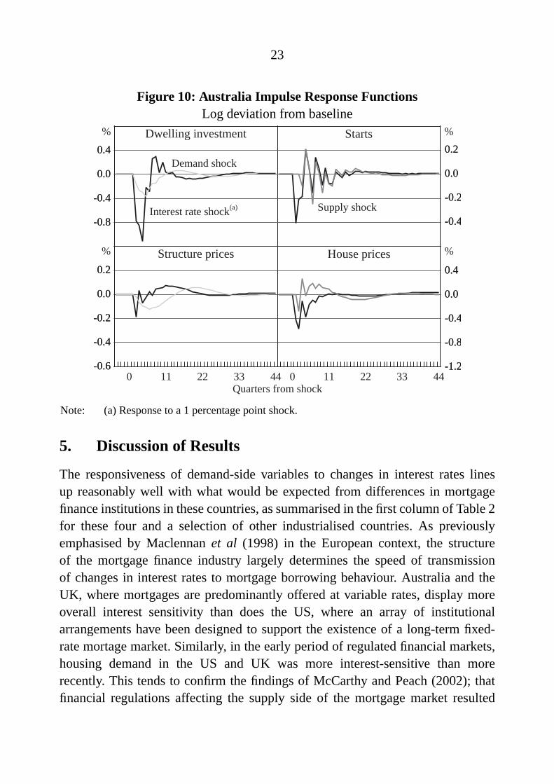
It is difficult to infer much about the behaviour of the housing sector from theraw econometric results, so we explore them using impulse responses. First, weinvestigate own-price elasticities by subjecting the supply equations to a demandshock (grey lines in the left-hand panels of Figures 5 to 10) and the demandequations to a supply shock (grey lines in the right-hand panels). The resultingresponses are analogous to slopes of supply and demand curves, although thedynamic nature of the equations implies that they are not direct representations ofeither short-run or long-run elasticities. If the demand shock engenders oscillationsin supply, we can furthermore diagnose the presence of intrinsic cyclicality.

18
Next, we explore the interest sensitivity of the sector by tracing out the effects ofa 1 percentage point shock to the policy interest rate (black lines in each panelof Figures 5 to 10). Since an increase in interest rates shifts both the demand andsupply schedules left, these dynamic responses confound slopes and shifts in thenotional curves implied by the econometric results. To ensure some comparabilitybetween the two sets of impulse responses, we have calibrated the supply anddemand shocks to be the same as the direct effects of a 1 percentage point shockto the policy rate on supply and demand respectively.8 All results are presented asthe log deviation from baseline, scaled up by a factor of 100; this can be interpretedas a percentage deviation from baseline.
Figure 5: US Impulse Response FunctionsPre-deregulation, log deviation from baseline
Quarters from shock
%
Structure prices House prices
Starts%
%%
-2
-1
0
1
-2
-1
0
1
-1
0
1
-1
0
1
-0.8
-0.4
0.0
-0.8
-0.4
0.0
-0.10
-0.05
0.00
0.05
-0.10
-0.05
0.00
0.05
Dwelling investment
444433220 11 33220 11
Interest rate shock(a)
Demand shockSupply shock
Note: (a) Response to a 1 percentage point shock.
8 That is, the shock is calibrated so that the direct, short-run effects are the same as for the interestrate shock. In the UK and the US, we shocked structure prices by 1 per cent even though interestrates did not enter that equation.

19
In the case of the US (Figures 5 and 6), there is no distinction between a demandshock and an interest rate shock, since in the preferred specification, interest ratesonly enter into the demand-side equations. That said, the results imply that supplyis more price-elastic than demand. The quantity response to a contractionarydemand shock or interest rate shock is greater than the apparent price response.In contrast, a contractionary supply shock results in a shift in demand that mainlychanges prices rather than quantities. The effect of an interest rate shock isaccordingly concentrated in quantities rather than prices, especially in the post-deregulation period. In line with the findings of McCarthy and Peach (2002), ourresults suggest that the housing demand in the US became less interest-sensitivefollowing the deregulation of the financial sector.
Figure 6: US Impulse Response FunctionsPost-deregulation, log deviation from baseline
Quarters from shock
%
Structure prices House prices
Starts%
%%
-2
-1
0
1
-2
-1
0
1
-1
0
1
-1
0
1
-0.2
0.0
0.2
-0.2
0.0
0.2
-0.10
-0.05
0.00
0.05
-0.10
-0.05
0.00
0.05
Dwelling investment
444433220 11 33220 11
Interest rate shock(a)
Demand shockSupply shock
Note: (a) Response to a 1 percentage point shock.

20
In contrast, the results for the UK are consistent with demand being more price-elastic than supply. Figures 7 and 8 show that a demand shock traces out a muchgreater price effect relative to the quantity effect on supply than is the case forthe effect of a supply shock on demand. Although confounded by the inclusionof public housing construction, this implies that the notional supply curve isrelatively steep, especially in the pre-deregulation period, which is consistent withthe overall pattern of housing construction moving relatively little over the courseof the cycle. It is therefore not surprising that both the price and quantity effectsof an interest rate shock are quite large relative to the results for the US.
Figure 7: UK Impulse Response FunctionsPre-deregulation, log deviation from baseline
Quarters from shock
%
Structure prices House prices
Starts%
%%
-0.6
-0.4
-0.2
0.0
-0.6
-0.4
-0.2
0.0
-1.0
-0.5
0.0
-1.0
-0.5
0.0
-0.6
-0.3
0.0
-0.6
-0.3
0.0
-0.3
-0.2
-0.1
0.0
-0.3
-0.2
-0.1
0.0
Dwelling investment
444433220 11 33220 11
Interest rate shock(a)
Demand shock
Supply shock
Note: (a) Response to a 1 percentage point shock.

21
Figure 8: UK Impulse Response FunctionsPost-deregulation, log deviation from baseline
Quarters from shock
%
Structure prices House prices
Starts%
%%
-0.6
-0.4
-0.2
0.0
-0.6
-0.4
-0.2
0.0
-1.0
-0.5
0.0
-1.0
-0.5
0.0
-0.6
-0.3
0.0
-0.6
-0.3
0.0
-0.3
-0.2
-0.1
0.0
-0.3
-0.2
-0.1
0.0
Dwelling investment
444433220 11 33220 11
Interest rate shock(a)
Demand shock Supply shock
Note: (a) Response to a 1 percentage point shock.
The results for Canada (Figure 9) are also consistent with a relatively flat (price-elastic) notional demand curve that shifts substantially in response to an interestrate shock. Unlike the UK, however, the total response to a change in interestrates is dominated by a quantity adjustment rather than a price adjustment. Thatis, the housing sector as a whole is more elastic in the face of shocks than itsUK counterpart. Indeed, of the four countries studied here, only in Canada doesthe effect of a move in interest rates weigh more heavily on structure prices (ps)than on the total price of established housing including land (ph). The impliedresponse of land prices must therefore be relatively subdued, which suggests thatland availability is less of a constraint on housing construction in Canada than inthe other countries studied here. This ties in with other evidence suggesting that thelevelof housing prices is relatively low in Canada (Ellis and Andrews 2001). Onereason for this might be that a greater proportion of the Canadian population livesin middle-sized cities where congestion costs are limited. This greater availabilityof land might contribute to the relatively elastic response of quantity supplied.

22
Figure 9: Canada Impulse Response FunctionsLog deviation from baseline
Quarters from shock
%
Structure prices House prices
Starts%
%%
-0.15
-0.10
-0.05
0.00
-0.15
-0.10
-0.05
0.00
-0.8
-0.4
0.0
-0.8
-0.4
0.0
-0.8
-0.4
0.0
-0.8
-0.4
0.0
-0.14
-0.07
0.00
0.07
-0.14
-0.07
0.00
0.07
Interest rate shock(a)
Demand shock
Supply shock
Dwelling investment
444433220 11 33220 11
Note: (a) Response to a 1 percentage point shock.
Finally, Figure 10 shows that only the Australian housing sector displayssignificant intrinsic cyclicality, as evidenced by the oscillations in quantitysupplied following a demand shock. Only the pre-deregulation period for theUS shows similar behaviour, and not to the same extent. Looking beyond thiscyclicality, it appears that both supply and demand in Australia are quite elastic,with the ratio of the price response to quantity response being comparable to theUS on the demand side, and Canada on the supply side. Similarly, the combinedeffect of a shock to interest rates on dwelling investment and house prices is thelargest of the four countries studied.
23
Figure 10: Australia Impulse Response FunctionsLog deviation from baseline
Dwelling investment
Structure prices House prices
Starts
Demand shock
%%
%%
Interest rate shock(a)
Quarters from shock
Supply shock
-1.2
-0.8
-0.4
0.0
0.4
-1.2
-0.8
-0.4
0.0
0.4
-0.6
-0.4
-0.2
0.0
0.2
-0.6
-0.4
-0.2
0.0
0.2
-0.8
-0.4
0.0
0.4
-0.8
-0.4
0.0
0.4
-0.4
-0.2
0.0
0.2
-0.4
-0.2
0.0
0.2
444433220 11 33220 11
Note: (a) Response to a 1 percentage point shock.
5. Discussion of Results
The responsiveness of demand-side variables to changes in interest rates linesup reasonably well with what would be expected from differences in mortgagefinance institutions in these countries, as summarised in the first column of Table 2for these four and a selection of other industrialised countries. As previouslyemphasised by Maclennanet al (1998) in the European context, the structureof the mortgage finance industry largely determines the speed of transmissionof changes in interest rates to mortgage borrowing behaviour. Australia and theUK, where mortgages are predominantly offered at variable rates, display moreoverall interest sensitivity than does the US, where an array of institutionalarrangements have been designed to support the existence of a long-term fixed-rate mortage market. Similarly, in the early period of regulated financial markets,housing demand in the US and UK was more interest-sensitive than morerecently. This tends to confirm the findings of McCarthy and Peach (2002); thatfinancial regulations affecting the supply side of the mortgage market resulted

24
in the demand side of the housing market being more interest-sensitive than ifthose lending restrictions had not been in place. In Canada, five-year fixed-ratemortgages predominate, consistent with its intermediate degree of responsivenessto interest rates.
Another aspect of the mortgage market that may be relevant to a reconciliationof demand-side behaviour is the tax treatment of mortgage interest. In theconsumption and asset demands framework outlined in Section 3.2, non-deductibility of mortgage interest implies that movements in interest rates have fullforce on user cost and the arbitrage conditions determining individuals’ demand,Equations (1) and (2). Therefore it should be expected that housing markets incountries where mortgage interest is not deductible for owner-occupiers shouldexperience larger effects of movements in interest rates. If this is true, then therecent completion of the abolition of mortgage interest deductibility in the UKshould be expected to result in a shift in demand behaviour to become moreinterest-sensitive than is presently the case.
Table 2: Housing Finance Institutions and Selected Demographic IndicatorsCountry Predominant
mortgagetype
Typicalmortgage term
(years)
Average annualpopulation growth
(1980–1998)
Populationdensity(2001)
Australia Adjustable 25 1.4 2.5
Canada Five-year fixed 25 1.2 3.3
US Full-term fixed 30 1.0 30.8
NZ Adjustable 25 1.1 14.3
France Five-year fixed 15 0.5 107.1
Germany Adjustable 10 0.3 230.5
Netherlands Adjustable 30 0.6 469.9
UK Adjustable 25 0.3 243.8
Japan Adjustable 30 0.4 348.1
Note: All variable, negotiable and reviewable interest rates are treated as adjustable.Sources: mortgage market characteristics – BIS (2003); demographic characteristics – World Bank
The patterns of interest sensitivity do not, however, completely line up with thedifferences in amplitudes of housing construction cycles identified in Section 2.Moreover, within this overall pattern of interest sensitivity, there are other cleardifferences, such as in the split between price and quantity responses. If themortgage characteristics were the only consideration, the responses of Australia

25
and the UK would be much more similar than they are. Two factors suggestthemselves as likely additional considerations in a reconciliation of these cross-country differences evident in Figures 1 and 2. Firstly, even economies withotherwise identical structures will experience different housing cycles if they facedifferent paths of interest rates, perhaps brought about for reasons other thandevelopments in the housing sector. And secondly, the split of the total responsebetween quantities and prices depends on the price elasticities of both demand andsupply, as well as on the extent to which demand shifts in response to a change ininterest rates.
As an illustration of this first point, we can use the models estimated in this paperto construct a counterfactual outcome for Australia that would have occurred hadthe United States’ path of interest rates prevailed instead. This counterfactualseries, shown in Figure 11 along with the actual series for both countries, iscalculated by replacing the actual Australian interest rate series with the USequivalent, and generating the fitted values that would have resulted, given ourestimated coefficients. Obviously this results in thelevel of housing investmentbeing higher than the actual outcome, since nominal interest rates were lower inthe US than in Australia for much of the period shown; we have not adjustedfor the fact that inflation was lower in the US than Australia in the 1980s.The counterfactual series is also smoother than the actual series for Australia,particularly for the 1980s, although still containing more obvious cycles in the1990s than the actual US series.
This exercise does not correspond to a true counterfactual: at the very least, incomealso responds to interest rates, and so the path of Australian income entering intohousing demand should also have been changed to fit the US interest rate series.This may reduce the cyclicality of the counterfactual Australian series further,since our econometric results also showed that the Australian housing sector wasrelatively income-sensitive. However, this would have required a structural modelof income that is beyond the scope of this paper. Even so, it is apparent fromFigure 11 that a significant part of the visual impression of regularity in thehousing construction cycle in Australia can be attributed to the greater cyclicalityof interest rates in the 1980s; the amplitude of the cycle around 2000 is more aresult of the introduction of the GST than changes in interest rates. This raisesthe possibility that, absent further changes to the tax system or other shocks,

26
Australian housing construction cycles might be more muted in the future thanwas the case historically.
Figure 11: Actual and Counterfactual Housing Construction
8.0
8.4
8.8
9.2
9.6
23.5
23.9
24.3
24.7
25.1
8.0
8.4
8.8
9.2
9.6
23.5
23.9
24.3
24.7
25.1
Australia actual(LHS)
200319981993198819831978
US actual(RHS)
Australia counterfactual(LHS)
Log Log
A more extensive illustration of the role of different paths of interest ratescan be obtained by eliminating interest rates from the model entirely. Table 3shows the changes in the variances of the endogenous variables that would ensuefrom holding interest rates constant at their sample means, given the estimatedparameters and the paths of the other exogenous variables. For each country, thevariances of the actual fitted values for the two quantity variables are greaterthan the variances of the counterfactual series where rates are held constant. Thisdemonstrates that interest rates have an important role in explaining constructioncycles: in particular, they appear to explain more of the variation in dwellinginvestment in Australia than in the US or UK, while housing starts are mostinterest-sensitive in the US. These results also imply that movements in interestrates have little exogenous effect on the variances of prices of housing andstructures.

27
It is also apparent from Table 3 that cross-country differences in housingoutcomes persist even when the influences of the path of rates, and consequentlythe differences in interest sensitivity, are removed. Because Table 3 comparesvariances of fitted values, these remaining cross-country differences are not dueto the contemporaneous effects of different shocks. They may partly relate tothe differences in the strength of the indirect influences of rates via the incomechannel, which as mentioned earlier, have not been removed in these results,as well as variation in other exogenous variables. However, it is also likely thatsome part of the cross-country differences can be attributed to different dynamicresponses of the endogenous variables once a shock has already occurred.
Table 3: Variance of Predicted and Counterfactual Endogenous VariablesEquation Australia Canada UK US(change in...) Fitted Counter- Fitted Counter- Fitted Counter- Fitted Counter-
factual factual factual factual
Dwelling investment 0.194 0.122 0.050 0.038 0.092 0.083 0.113 0.096
Starts 0.438 0.390 0.393 0.359 0.394 0.357 0.215 0.138
Structure prices 0.016 0.013 0.009 0.010 0.031 0.037 0.004 0.005
House prices 0.070 0.056 0.029 0.032 0.045 0.048 0.007 0.010
Notes: Interest rates are held constant at their mean rate in the counterfactual. All variances have been multipliedby 100 to be expressed in percentage points.
This underlines the importance of the second factor mentioned earlier – the role ofdifferences in price elasticities. This can be seen by comparing this paper’s resultsfor the UK and Australia. In both countries, housing demand is quite interest-sensitive, as well as being quite price-elastic. However, as shown in Figure 1,housing construction is almost completely acyclical in the UK, in contrast to theclear cycles seen in the Australian data, and the impulse response of quantitiesto interest rate shocks shown in Figures 7 and 8 is likewise much smaller thanin either Australia or the US. What appears to be happening is that in the UK,transmission of changes in interest rates to credit markets is similar to that inAustralia, but the onward transmission from that market is via housingpricestoother aspects of consumer behaviour, rather than directly to physical investmentin housing. This suggests the presence of a steep supply curve, or some rigiditycausing the adjustment in the UK to come through price rather than quantity. Thisis confirmed by the impulse response analysis: as mentioned in Section 4, theeconometric results imply that the notional supply curve is quite steep.

28
The last two columns in Table 2 provide a hint of the underlying reason forthis inelasticity in supply. The UK – and indeed most of continental Europe– is characterised by slow population growth and high population density, incontrast to the situation in Australia, Canada and the US. A given-sized cyclicalshift in demand represents a proportionately larger shift compared to the loweraverage levels of construction activity that might be expected in a country withlow population growth. This might entail greater costs of adjustment than if theshift in production was only small relative to the size of the industry. In otherwords, adjustment costs might provide reasons for construction supply curves tobe fairly steep in countries where construction is small relative to its importancein other countries. Given the likely constraints imposed by population densityand thus land scarcity, the preponderance of price adjustment rather than quantityadjustment in the UK seems entirely consistent with the characteristics of thatmarket. If countries in continental Europe with a similar supply environment hadmortgage markets like that of the UK, one might also expect them to experiencesimilar variability in housing prices.
Another possible contributor to the greater amplitude of housing constructioncycles in Australia may be the apparent intrinsic cyclicality identified in theimpulse response analysis for Australia, but not elsewhere. Since some of theestimated parameters in these models are imprecisely estimated, it would be amistake to make much of the finding that only Australia’s housing sector exhibitsintrinsic cyclicality in the face of a simple demand shock. This finding could,however, be another factor explaining the differences shown in Figures 1 and 2.It is also important to note that intrinsic cyclicality does not imply that supplyis inelastic. Rather, intrinsic cyclicality is likely to occur when both demand andsupply are quite elastic, but supply is sluggish; that is, the short-run elasticity ismuch lower than the supply elasticity in the medium to long run. By comparison,the sticky supply evident in the results for the UK imply that construction doesnot respond much to a shock over any horizon. In that case, there is not enoughvariation in quantity for an intrinsic cycle to get started.
Although mortgage finance conventions are not the only factors drivingdifferences in the interest sensitivity of housing construction, they have animportant role. This naturally raises the question of why the deregulated outcomesfor financediffer so much. Presumably households in all four countries wouldvalue the reduced volatility of payments inherent in a fully fixed-rate loan contract,

29
but only in the US do a significant proportion of households pay for this reducedvolatility. A full investigation of the reasons for this difference is beyond the scopeof this paper. However, one of the key contributors to this difference appears to bethe substantial involvement of government-sponsored agencies in the US mortgagemarket. The financing advantages of these institutions reduce the term premiumthat US households must pay for a fixed-rate loan over a variable-rate loan over thewhole term. Additionally, the differences in tax treatment mentioned earlier mayalso be relevant. The incentive to pay off their mortgage ahead of schedule is muchstronger in a country where home mortgage interest is not tax-deductible, such asAustralia, since alternative uses of funds earn a post-tax, not pre-tax, return. Thismakes variable-rate loans relatively more attractive, since unlike fixed-rate loans,they do not generally involve penalties for early repayment.
6. Conclusion
In this paper, we have estimated structural models of housing supply and demandfor several countries. The separate treatment of number and quality of dwellingshas allowed us a reasonable identification of the two sides of the market, andpointed towards some possible reasons for differences between the behaviour ofthe housing markets in these countries. With only four countries in our data set,it is not possible to demonstrate conclusively that these cross-country differencesare the results of the institutional and other differences discussed in the previoussection, but they are likely to be important parts of the story.
In particular, the results for the UK seem to indicate that countries with supplyconstraints on land and generally slow population growth might have housingconstruction cycles with lower amplitude than those in countries where populationgrowth is relatively higher and where there is more scope to expand residentialdevelopment. If housing demand displayed similar interest sensitivity in allcountries, we should expect that movements in rates would be translated moreinto price than volume movements in countries where these supply constraints areimportant. Notwithstanding recent developments in housing prices in Australiaand elsewhere, we should therefore expect both structure and land prices to belesscyclical (and quantities more cyclical) on average in countries like Australiaand the US than in continental Europe or Japan. It should also be expected thatcycles in quantities would be more a feature of the Australian data, while the UK,
30
with otherwise similar institutions in the mortgage market, would be more subjectto cycles in housing prices.
Institutional details in the housing finance market also have a role in explainingthe differing behaviour of construction and housing prices across countries andthrough time, and considerably complicate the story. The details of taxationarrangements and government intervention in the housing market might also makea difference, by determining where on the yield curve the mortgage market tendsto operate.
We have estimated reasonably consistent, structurally motivated models forhousing construction activity for a range of developed countries. However, thesemodels do differ, and would be likely to have differed more if we had been trying totune the individual country models closer to the data in each country. Quantitativefindings about construction behaviour and policy transmission in one country aretherefore likely to be inapplicable for other countries with different institutions.Although we have drawn out several likely factors explaining the differences incyclicality and interest sensitivity in housing construction across countries, it ispossible that these are not the only ones. Further research on these differenceswould therefore seem desirable in order to know whether lessons from one countryare applicable to another.

31
Appendix A: Data Sources
Table A1: Data DefinitionsSeries Definition
Dwelling investment Gross fixed capital formation in dwellings at constant prices
Structure prices Implicit price deflator for GFCF in dwellings
House prices Median/mean price of dwellings at current prices
Housing starts Number of new residential building starts
Housing stock Total stock of dwellings
Number of households Total number of households
Permanent income Sum of non-durables and services consumption at constant prices
General price level Level of the consumer price index
Construction costs Weighted average of house building materials prices and labourcosts at current prices
Policy interest rate Interest rate targeted by central bank
Notes: The consumer price index for Australia excludes the effect of the GST. The weights for the constructioncost variables are taken from countries’ input-output tables. In the UK, we use household consumptionexpenditure as a proxy for permanent income. Some housing and demographic data are only available forGreat Britain (i.e. excluding Northern Ireland) rather than for the entire UK. We have therefore had torescale and interpolate these data to obtain a consistent data set for the UK. Details of these adjustmentsare available from the authors.
Table A2: Statistical SourcesAbbreviation Full title
ABS Australian Bureau of Statistics
BEA Bureau of Economic Analysis
BLS Bureau of Labor Statistics
BIS Bank for International Settlements
CB US Census Bureau
CMHC Canada Mortgage and Housing Corporation
DTI UK Department of Trade and Industry
NAR National Association of Realtors
NIDSD Northern Ireland Department of Social Development
ODPM Office of the Deputy Prime Minister

32
Table A3: Data SourcesSeries Australia Canada UK US
Dwellinginvestment
ABS Cat No5206.0
Stat Can038-0010
NSDFEG BEA
Structure prices ABS Cat No5206.0
Stat Can038-0010
NSDFEG,DFDK
BEA
House prices CBA/HIA;CommonwealthTreasury; REIA
BIS Nationwide NARmed.existing 1-familyhomes
Housing starts ABS Cat No5750.0, 5752.0
CMHC ODPM211; NSFCAB, CTOR,CTOV
CB C20
Housing stock ABS Cat No5752.0, Census
Stat Canv227368;CMHC
ODPM 101, 241;NSFCAB, CTOR,CTOV
CB HousingVacancy Survey 7
Number ofhouseholds
ABS Cat No3101.0, Census
Stat Canv227374 ODPM 401;NIDSD
CB HousingVacancy Survey 7
Permanentincome
ABS Cat No5206.0
Stat Can380-0009
NSABJR BEA
Generalprice level
ABS Cat No6401.0; RBA
Stat Canv735319 NSCHAW BLSCUSR0000SA0
Constructioncosts
ABS Cat No6427.0, 6302.0,5209.0
Stat Canv734362,v4331335,v4331326,329-0038
NSLabourMarket TrendsE.2, LNMQ; DTI
BLS wpusop2200,EEU20152006
Policyinterest rate
RBA Bank of Canada Bank of England Federal Reserve
Notes: See Table A2 for abbreviations. Relevant catalogue, series and table identifiers are italicised. All series areseasonally adjusted, using conventional methods in Eviews where necessary. For consistency, annualiseddata are converted to quarterly values where appropriate.

33
Appendix B: Econometric Results
In the panel showing results for the dynamics, the numerical entries denote thesum of the coefficients on current values and lags of that variable. Where morethan one lag of a variable is included, the sign of the first coefficient (current-dated or shortest lag) is shown as a subscript on the summation. The orders ofthe lags used are shown in parentheses alongside the reported coefficient sum.The significance levels of the first coefficient in the dynamics and of the long-runcoefficients at the 10, 5 or 1 per cent levels are indicated by superscripted∗, ∗∗or †.
To conserve space and make interpretation easier, we report individual coefficientsonly for the long-run relationships in each equation. We report the sumof the coefficients on dynamic terms for each variable, with the range ofcontemporaneous or lagged variables indicated in parentheses alongside thissummation. Sequences of lagged explanators can sometimes include coefficientswith different signs, or where intermediate lags are not significant. We thereforealso report the sign and significance of the estimated coefficient on the lowest lagof each variable as subscripts and superscripts to the sum of the coefficients.

34
Table B1: System Results – AustraliaEquation Supply mark-up Total supply Quantity demand House prices
Dependent variable ∆sp ∆hc ∆s ∆hp
Long-run variables (t−1-dated)
Starts (s) 0.02† − −0.14† −Construction (hc) − −0.17† − −Costs(cc) 0.07† − − −Housing prices(hp) 0.02∗∗ 0.14∗∗ − −0.12†
Structure prices(sp) −0.11† −0.09 − −Interest rates(i) − −0.00 − −Income(y) − − − 0.16†
CPI (p) − −0.05 − 0.12†
Vacancy rate(v) − − −3.42† −1.56∗∗
Household growth(hh) − − 0.04 −Dynamics
∆s − − 0.51†+ (4–6) −
∆hc − 0.17∗∗ (1) − −∆cc −0.33†
− (4–5) − − −∆hp 0.19†
+ (2–3) 0.19∗∗+ (1–6) −0.46∗∗ (6) −0.24† (1)
∆sp 0.52†+ (2–3) 0.15∗+ (2–6) −0.31∗∗+ (1–4) 1.61† (0)
Interest rates 0.09†− (2–3) −0.21∗∗− (2–5) −0.68† (1) −0.42† (1)
∆y − − −10.48†− (1–5) −0.74† (5)
∆p − −0.60∗ (6) −2.43† (2) 0.55∗∗ (3)
∆v − − −23.28∗∗− (1–4) −8.25† (3)
∆hh − − −0.12∗∗ (3) −GST dummy 0.08† (0) −0.13∗+ (4– -1) −0.11†
+ (4–0) −0.30† (0)
Post-GST dummy 0.01∗∗ − − −Constant −0.31† 0.52∗ 1.20† −0.89†
R-bar squared 0.83 0.70 0.71 0.54
Breusch-Godfrey LM 4.24 −0.59 −0.12 3.95
Jarque-Bera 87.61 96.15 0.54 0.36
Notes: Estimated 1975:Q4–2003:Q3. The GST dummy takes the value 1 for the 2000:Q3. The time indicatorsfor the GST dummy refer to leads. The post-GST dummy takes the value 1 for every observation from2000:Q3. Instruments for endogenous variables included lags of endogenous variables, construction costsand permanent income.

35
Table B2: System Results – United KingdomEquation Supply mark-up Total supply Quantity demand House prices
Dependent variable ∆sp ∆hc ∆s ∆hp
Long-run variables (t−1-dated)
Starts(s) 0.02 − −0.45† −Construction(hc) − −0.54† − −Costs(cc) 0.24† − − −Housing prices(hp) 0.14† −0.10 − −0.02∗
Structure prices(sp) −0.37† 0.73† − −Interest rates(i) − 0.11† − −CPI (p) − −0.74† − 0.02∗
Vacancy rate(v) − − −4.90† 0.13
Household growth(hh)I − − −0.15† −Household growth(hh)II − − 0.07 −
Dynamics
∆s I 0.09∗∗ (4) − − 0.17†+ (0–4)
∆s II − − − 0.17†+ (0–4)
∆hc − 0.92†+ (3–6) − −
∆cc I 0.43∗∗ (5) − − −∆hp I −0.03∗∗− (1–6) 1.58∗∗+ (2–6) −1.94† (4) 0.60†
+ (1–3)
∆hp II −0.29∗∗ (2) 1.58∗∗+ (2–6) − 0.60† (1–3)
∆spI 0.37∗∗+ (2–4) −3.59†− (1–4) 0.49∗∗ (4) −
∆spII 0.41† (4) −2.64†− (1–3) − −
Interest rates I − −0.81† (2) −2.35† (2) −0.23† (2)
Interest rates II − −0.40∗∗ (2) 0.62∗ (5) −0.23† (2)
∆y I − − 1.244†+ (2–3) 0.93∗∗+ (0–4)
∆y II − − 10.00∗∗+ (0–3) 0.93∗∗+ (0–4)
∆p I − 0.99†+ (1–6) 1.79∗∗ (3) 0.39†
+ (0–1)
∆p II − 1.29† (1) − 0.39†+ (0–1)
1979 dummy − − −0.31† −Constant I −1.18† 13.73† 7.03† 0.10∗∗
Constant II −1.18† 13.73† 4.11† 0.10∗∗
R-bar squared 0.59 0.43 0.36 0.64
Breusch-Godfrey LM 4.81 1.12 4.98 −3.87
Jarque-Bera 22.02 625.84 10.42 9.33
Notes: Estimated 1971:Q4–2003:Q2. Instruments for endogenous variables included lags of endogenous variables,construction costs and permanent income. A structural break is allowed for in 1986:Q1. Coefficients thatapply only to the first segment of the data are labelled I, while those applying only in the second segmentare labelled II. Dummy for 1979:Q1 to capture significant fall in starts.

36
Table B3: System Results – United StatesEquation Supply mark-up Total supply Quantity demand House prices
Dependent variable ∆sp ∆hc ∆s ∆hp
Long-run variables (t−1-dated)
Starts(s) 0.00 − −0.10† −Construction(hc) − −0.19† − −Costs(cc) 0.04 − − −Housing prices(hp) 0.04∗ 0.22 − −0.07†
Structure prices(sp) −0.06∗∗ 0.05 − −Interest rates(i) − −0.02† − −Income(y) − − − 0.09†
CPI (p) − −0.25∗∗ − 0.07†
Vacancy rate(v) − − −1.53 −0.11
Household growth(hh) − − 0.01 −Dynamics
∆s − − −0.12 (3) −∆cc II −0.30∗ (0) − − −∆hc I − 0.13†
+ (1–4) − −∆hc II − 0.37†
+ (1–2) − −∆hp I 0.58†
+ (2–3) 6.42†+ (2–6) −3.08† (0) 0.33† (5)
∆hp II − − −1.79∗ (4) −∆spI − −4.15− (3–6) − 0.867†
+ (0–3)
∆spII − −1.56∗ (0) − 1.27†+ (2–5)
Interest rates(i) I − −0.08†− (2–3) −1.18† (0) −0.08† (3)
Interest rates(i) II − − −1.46† (2) 0.14†− (5–6)
∆y II − − − −0.69†+ (0–2)
∆p I − −6.16†− (0–4) −1.17†
− (1–4) −∆p II − −6.16†
− (0–4) − −0.27†− (3–4)
∆v II − − − 0.79∗∗ (2)
Constant I −0.29∗∗ 3.25† 1.36† −0.34†
Constant II −0.29∗∗ 3.25† 1.36† −0.36†
R-bar squared 0.47 0.51 0.14 0.53
Breusch-Godfrey LM 0.84 4.99 4.66 2.01
Jarque-Bera 408.20 37.21 2.22 0.48
Notes: Estimated 1967:Q3–2003:Q2. Instruments for endogenous variables included lags of endogenous variables,construction costs and permanent income. A structural break is allowed for in 1986:Q1. Coefficients thatapply only to the first segment of the data are labelled I, while those applying only in the second segmentare labelled II.

37
Table B4: System Results – CanadaEquation Supply mark-up Total supply Quantity demand House prices
Dependent variable ∆sp ∆hc ∆s ∆hp
Long-run variables (t−1-dated)
Starts(s) −0.02† − −0.42† −Construction(hc) − −0.07∗∗ − −Costs(cc) 0.09† −0.09 − −Housing prices(hp) 0.14† −0.18∗∗ − −0.06†
Structure prices(sp) −0.27† 0.22 − −Interest rates(i) − 0.00∗∗ − −Income(y) − − − −CPI (p) − 0.03 − 0.06†
Vacancy rate(v) − − −5.10† −0.32
Household growth(hh) − − 0.25† −Dynamics
∆s 0.02† (1) − −0.16∗∗ (4) −∆hc − −0.18†
+ (1–4) − −∆cc −0.47∗+ (2–4) −1.56† (1) − −∆hp 0.37†
+ (0–3) 2.29†+ (0–5) 2.17†
+ (1–2) 0.31† (4)
∆sp 0.37∗∗+ (1–4) −2.21†− (1–4) −1.42∗ (4) −
Interest rates −0.00∗∗+ (1–2) −0.01† (0) −0.01† (0) −0.00 (3)
∆y − − 4.00† (3) 2.22∗∗+ (0–3)
∆p − 1.49† (2) 5.57† (2) −∆v − − 35.59† (1) −10.09† (3)
GST dummy 0.04† −0.06∗∗ − 0.10†
GST dummy (-1) − − − 0.09†
Post-GST dummy −0.01∗∗ − − −Constant 0.41† 1.50∗∗ 2.13† 0.05∗
R-bar squared 0.74 0.63 0.52 0.36
Breusch-Godfrey LM 1.63 −0.37 −0.17 1.68
Jarque-Bera 0.50 0.72 3.49 0.78
Notes: Estimated 1976:Q4–2003:Q3. GST dummy takes the value 1 for the 1990:Q1. The post-GST dummy takesthe value 1 for every observation from 1990:Q1. Instruments for endogenous variables included lags ofendogenous variables, construction costs and permanent income.

38
References
Abraham JM and PH Hendershott (1996), ‘Bubbles in metropolitan housingmarkets’,Journal of Housing Research, 7(2), pp 191–207.
Andrews DWK (1993),‘Tests for parameter instability and structural change withunknown change point’,Econometrica, 61(4), pp 821–856.
Aoki K, J Proudman and G Vlieghe (2002),‘Houses as collateral: has the linkbetween house prices and consumption in the U.K. changed?’, Federal ReserveBank of New YorkEconomic Policy Review, 8(1), pp 163–177.
Attanasio OP and G Weber (1994),‘The UK consumption boom of the late1980s: aggregate implications of microeconomic evidence’,Economic Journal,104(427), pp 1269–1302.
Bai J, RL Lumsdaine and JH Stock (1998), ‘Testing for and datingcommon breaks in multivariate time series’,Review of Economic Studies, 65(3),pp 395–432.
(BIS) Bank for International Settlements (2003),‘Turbulence in asset markets:the role of micro policies’, Report of the Contact Group on Asset Prices.
Bourassa SC and PH Hendershott (1992),‘Over-investment in Australianhousing?’, National Housing Strategy Background Paper No 9.
Bourassa SC and PH Hendershott (1995),‘Australian capital city real houseprices, 1979–1993’,Australian Economic Review, 111(3), pp 16–26.
Chinloy P (1996),‘Real estate cycles: theory and empirical evidence’,Journal ofHousing Research, 7(2), pp 173–190.
Edey M and K Hviding (1995), ‘An assessment of financial reform in OECDcountries’, OECD Economics Department Working Paper No 154.
Egebo T, P Richardson and I Lienert (1990),‘A model of housing investmentfor the major OECD economies’,OECD Economic Studies, 14, pp 151–188.
Ellis L and D Andrews (2001), ‘City sizes, housing costs and wealth’, ReserveBank of Australia Research Discussion Paper No 2001-08.

39
Gallin J (2003), ‘The long-run relationship between house prices and income:evidence from local housing markets’, Federal Reserve Board of GovernorsFinance and Economics Discussion Series No 2003-17.
Glaeser EL and J Gyourko (2002), ‘The impact of zoning on housingaffordability’, Harvard Institute of Economic Research Discussion Paper No 1948.
Henderson JV and YM Ioannides (1983),‘A model of housing tenure choice’,American Economic Review, 73(1), pp 98–113.
Henderson JV and YM Ioannides (1986),‘Tenure choice and the demand forhousing’,Economica, 53(210), pp 231–246.
Ioannides YM and SS Rosenthal (1994),‘Estimating the consumption andinvestment demands for housing and their effect on housing tenure status’,Reviewof Economics and Statistics, 76(1), pp 127–141.
Kenny G (1999),‘Modelling the demand and supply sides of the housing market:evidence from Ireland’,Economic Modelling, 16(3), pp 389–409.
Lessard D and F Modigliani (1975),‘Inflation and the housing market: problemsand potential solutions’,Sloan Management Review, 17(1), pp 19–35.
Maclennan D, J Muellbauer and M Stephens (1998),‘Asymmetries in housingand financial market institutions and EMU’,Oxford Review of Economic Policy,14(3), pp 54–80.
McCarthy J and RW Peach (2002),‘Monetary policy transmission to residentialinvestment’, Federal Reserve Bank of New YorkEconomic Policy Review, 8(1),pp 139–158.
Meen GP (1990),‘The removal of mortgage constraints and the implications foreconometric modelling of UK house prices’,Oxford Bulletin of Economics andStatistics, 52(1), pp 1–23.
Meen GP (2000),‘Housing cycles and efficiency’,Scottish Journal of PoliticalEconomy, 47(2), pp 114–140.
Ortalo-Magne F and S Rady (1999),‘Boom in, bust out: young households andthe housing price cycle’,European Economic Review, 43(4–6), pp 755–766.

40
Rosenthal SS (1999),‘Residential buildings and the cost of construction: newevidence on the efficiency of the housing market’,Review of Economics andStatistics, 81(2), pp 288–302.
Stein JC (1995),‘Prices and trading volume in the housing market: a model withdown-payment effects’,Quarterly Journal of Economics, 110(2), pp 379–406.
Stevens GR (1997),‘Some observations on low inflation and household finances’,Reserve Bank of AustraliaBulletin, October, pp 38–47.
Sutton GD (2002),‘Explaining changes in house prices’,BIS Quarterly Review,pp 46–55.
Throop AW (1986), ‘Financial deregulation, interest rates, and the housing cycle’,Federal Reserve Bank of San FranciscoEconomic Review, 1986(3), pp 63–78.
Topel R and S Rosen (1988),‘Housing investment in the United States’,Journalof Political Economy, 96(4), pp 718–740.
Tsatsaronis K and H Zhu (2004),‘What drives housing price dynamics: cross-country evidence’,BIS Quarterly Review, pp 65–78.