hourglassstabilizationandthevirtualelementmethoddilbert.engr.ucdavis.edu/~suku/polyfem/papers/vem-hourglass-2015.pdf ·...
TRANSCRIPT

INTERNATIONAL JOURNAL FOR NUMERICAL METHODS IN ENGINEERING
Int. J. Numer. Meth. Engng 2014; 1:1–33 Prepared using nmeauth.cls [Version: 2000/01/19 v2.0]
Hourglass stabilization and the virtual element method
A. Cangiani1, G. Manzini2,3,4, A. Russo3,5 and N. Sukumar6,∗
1 Department of Mathematics, University of Leicester, University Road – Leicester LE1 7RH, UK
2 Theoretical Division, Los Alamos National Laboratory, Los Alamos, NM 87545, USA
3 Istituto di Matematica Applicata e Tecnologie Informatiche del CNR, via Ferrata 1, 27100 Pavia, Italy,
4 Centro per la Simulazione Numerica Avanzata, Istituto Universitario di Studi Superiori, 27100 Pavia, Italy
5 Dipartimento di Matematica e Applicazioni, Universita di Milano-Bicocca, 20153 Milano, Italy
6 Department of Civil and Environmental Engineering, University of California, Davis, CA 95616, USA
SUMMARY
In this paper, we establish the connections between the virtual element method (VEM) and the
hourglass control techniques that have been developed since the early 1980s to stabilize underintegrated
C0 Lagrange finite element methods. In the virtual element method, the bilinear form is decomposed
into two parts: a consistent term that reproduces a given polynomial space and a correction term that
provides stability. The essential ingredients of C0-continuous virtual element methods on polygonal
and polyhedral meshes are described, which reveals that the variational approach adopted in the VEM
affords a generalized and robust means to stabilize underintegrated finite elements. We focus on the
heat conduction (Poisson) equation, and present a virtual element approach for the isoparametric
four-node quadrilateral and the eight-node hexahedral element. In addition, we show quantitative
∗Correspondence to: N. Sukumar, Department of Civil and Environmental Engineering, University of California,
One Shields Avenue, Davis, CA 95616, USA. E-mail: [email protected]
Copyright c© 2014 John Wiley & Sons, Ltd.
2 CANGIANI ET AL.
comparisons of the consistency and stabilization matrices in the VEM to those in the hourglass
control method of Belytschko and coworkers. Numerical examples in two and three dimensions are
presented for different stabilization parameters, which reveals that the method satisfies the patch test,
and delivers optimal rates of convergence in the L2 norm and the H1 seminorm for Poisson problems
on quadrilateral, hexahedral, as well as arbitrary polygonal meshes. Copyright c© 2014 John Wiley
& Sons, Ltd.
key words: virtual element method, underintegration, hourglass control, consistency matrix,
stabilization matrix, polygonal and polyhedral finite elements
1. INTRODUCTION
For linear and nonlinear transient analysis, underintegrated finite elements (FE) with hourglass
stabilization is widely adopted. There are little benefits to using the full tensor-product Gauss
quadrature (2 × 2 for bilinear quadrilateral elements and 2 × 2 × 2 for trilinear hexahedral
elements): apart from the increased computational costs that are incurred, these elements are
also prone to locking for incompressible materials for which some form of reduced integration
is desirable. Hence, use of the one-point quadrature, combined with some form of stabilization,
has been a topical area of research since the early 1980s. This feature is available in many of
the finite element software codes [1–5].
Use of the one-point quadrature leads to a rank-deficient (singular) stiffness matrix and
the presence of hourglass (solid continua) or spurious singular (Poisson equation) modes. This
rank-deficiency is cured by the addition of a second matrix, the so-called hourglass stabilization
matrix, which suppresses the spurious singular modes. Early studies to address this issue
for low-order finite elements are due to Key [6] and Kosloff and Frazier [7]. To speed up
Copyright c© 2014 John Wiley & Sons, Ltd. Int. J. Numer. Meth. Engng 2014; 1:1–33
Prepared using nmeauth.cls

HOURGLASS STABILIZATION AND THE VIRTUAL ELEMENT METHOD 3
finite element computations, Flanagan and Belytschko [8] introduced the notion of orthogonal
hourglass control, which was further extended and refined by them in subsequent studies [9–11].
In the literature, following Reference [8], many other initial contributions related to hourglass
stabilization have also appeared [12–14]; for a historical perspective and an exhaustive list of
references on this topic, the interested reader can see References [10, 15].
In this paper, we restrict our attention to the scalar diffusion (Poisson) problem, and draw
connections with the formulations presented in References [8–10]. In keeping with the usage in
the literature for problems in solid continua, we choose to use the term hourglass when referring
to issues that pertain to the nonphysical modes of the stiffness (conductance) matrix. In
Belytschko et al. [10], hourglass projection is obtained by using the consistency requirements
and enforcing the elimination of the rank-deficiency of the discrete forms. Herein, we show
that the recently proposed virtual element method [16], coined as VEM, can be viewed as
a generalized hourglass stabilization technique for arbitrary-order polygonal and polyhedral
finite element methods. In Section 4, the key properties of isoparametric finite elements in two-
and three-dimensions are reviewed. In Section 5, we discuss reduced integration techniques
for the Poisson problem recalling the well-known mean-gradient approach of Belytschko and
coworkers [8–10]. The framework for first-order virtual elements is presented in Section 6.
In Section 7, we show that virtual element discretizations can be constructed on general (convex
and nonconvex) polygons and polyhedra and we provide a simple formula for the computation
of the stiffness matrix. The derivation of the VEM for the bilinear isoparametric four-node
quadrilateral element is presented in Section 8, and direct comparisons to the approach of
Belytschko and coworkers [8–10] are made. The trilinear isoparametric eight-node hexahedral
element is treated in Section 9, where quantitative links between the VEM and the hourglass
Copyright c© 2014 John Wiley & Sons, Ltd. Int. J. Numer. Meth. Engng 2014; 1:1–33
Prepared using nmeauth.cls

4 CANGIANI ET AL.
control method in References [8, 10] are also established. In general, isoparametric eight-node
hexahedral elements have curved faces and this paper provides an implementation for them.
Numerical examples presented in Section 10 confirm that the VEM satisfies the patch test and
achieves optimal rates of convergence in the L2 norm and in the H1 seminorm on quadrilateral,
hexahedral, as well as polygonal meshes. We conclude with some final remarks in Section 11.
2. NOTATION
Let us summarize the main notations used in this paper. The symbol d represents the spatial
dimension, which is either 2 or 3. Bold symbols like s, X, K represent vectors or matrices.
A point x ∈ IRd is denoted as x ≡ (x, y) in two-dimensions and as x ≡ (x, y, z) in three
dimensions. The symbol Ω0 denotes either the biunit reference square (−1, 1)2 or the biunit
reference cube (−1, 1)3, and Ωe is the physical element, which is a quadrilateral or hexahedral
finite element. The isoparametric four-node or eight-node finite element space on Ωe is written
as Q1(Ωe). Note that hexahedra can have curved faces.
A general finite element is denoted by the letter E and the finite element space attached to
it is written as V Eh . The number of vertices of E is denoted by nE , which is also the dimension
of V Eh because the degrees of freedom of the finite elements considered in this paper are always
associated with the vertices. The diameter of an element E is denoted by hE and its area (or
volume) by |E|; when E = Ωe, we use he instead of hΩe. The space of polynomials of degree
less than or equal to k on E is denoted by Pk(E).
Copyright c© 2014 John Wiley & Sons, Ltd. Int. J. Numer. Meth. Engng 2014; 1:1–33
Prepared using nmeauth.cls

HOURGLASS STABILIZATION AND THE VIRTUAL ELEMENT METHOD 5
3. THE POISSON PROBLEM
For the sake of simplicity, we consider the following Poisson problem with nonhomogeneous
Dirichlet boundary conditions:
−∆u = f in Ω ⊂ IRd (1a)
u = g on ∂Ω, (1b)
where d = 2, 3 is the spatial dimension and f is a forcing function. The bilinear form associated
with problem (1) is denoted by a(·, ·):
a(u, v) :=
∫
Ω
∇u · ∇v dx. (2)
If E ⊂ Ω is a generic finite element, we denote by aE(·, ·) the restriction of a(·, ·) to E; that is,
aE(u, v) :=
∫
E
∇u · ∇v dx,
with∑
E aE(u, v) = a(u, v).
The numerical approximation of aE(·, ·) is denoted by aEh (·, ·), and the corresponding global
approximation ah(·, ·) of a(·, ·) is defined as
ah(u, v) :=∑
E
aEh (u, v).
If V Eh is the finite element space attached to E and φ1, . . . φnE
are the Lagrange shape
functions, the exact nE × nE element stiffness matrix KE is given by
(KE)ij := aE(φi, φj) :=
∫
E
∇φi · ∇φj dx i, j = 1, . . . , nE .
The stiffness matrix corresponding to aEh (·, ·) is defined as
(KEh
)ij:= aEh (φi, φj) i, j = 1, . . . , nE .
The superscript E and the subscript h will be often omitted when no confusion can arise.
Copyright c© 2014 John Wiley & Sons, Ltd. Int. J. Numer. Meth. Engng 2014; 1:1–33
Prepared using nmeauth.cls
6 CANGIANI ET AL.
3.1. Linear consistency and stability
We consider spaces V Eh that contain linear polynomials and other functions that are not linear.
In order to guarantee stable and convergent approximations, we say that aEh (·, ·) is
(i) linearly consistent if it is exact when one of the two entries is a linear polynomial:
aEh (uh, p1) = aE(uh, p1) for all uh ∈ V Eh , p1 ∈ P1(E). (3)
(ii) stable if it is uniformly bounded from above and below by the exact bilinear form
aE(·, ·):
there exist two constants α∗ and α∗ independent of h such that
α∗aE(vh, vh) ≤ aEh (vh, vh) ≤ α∗aE(vh, vh) for all vh ∈ V E
h .
(4)
The two properties defined above guarantees that the method passes the patch test, which we
state as a Theorem for future reference in this paper.
Theorem 1. Let the approximate bilinear form aEh (·, ·) be linearly consistent (3) and
stable (4). Then, the corresponding Galerkin method passes the linear patch test.
4. LOW-ORDER ISOPARAMETRIC ELEMENTS IN 2D AND 3D
Let us recall the essential properties of the four-node quadrilateral and the eight-node
hexahedral isoparametric finite elements.
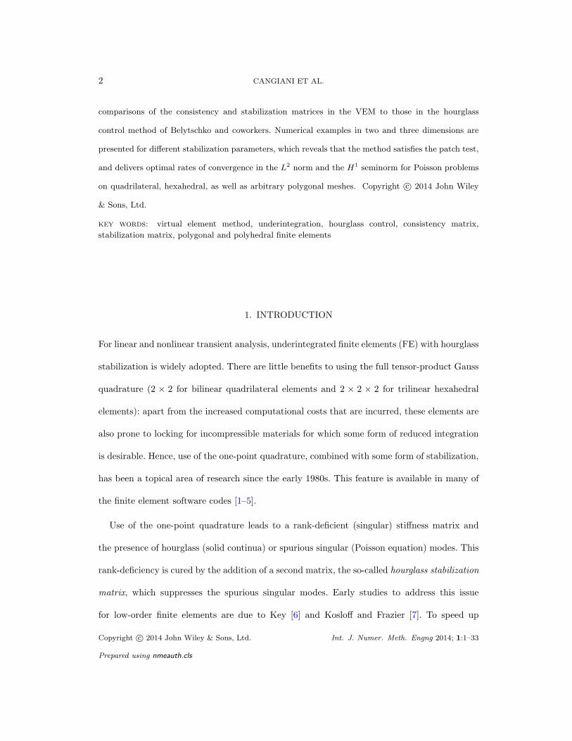
4.1. Quadrilateral element
Let Ωe be a convex quadrilateral with vertices xi = (xi, yi), i = 1, . . . , 4, and Ω0 = (−1, 1)2
be the reference biunit square. Its vertices ξi = (ξi, ηi), i = 1, . . . , 4, are ordered as follows:
ξ1 = (−1,−1), ξ2 = (+1,−1), ξ3 = (+1,+1), ξ4 = (−1,+1).
Copyright c© 2014 John Wiley & Sons, Ltd. Int. J. Numer. Meth. Engng 2014; 1:1–33
Prepared using nmeauth.cls
HOURGLASS STABILIZATION AND THE VIRTUAL ELEMENT METHOD 7
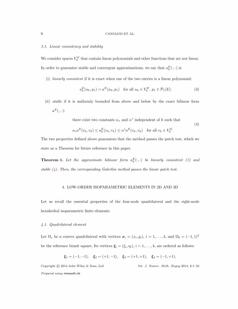
The bilinear isoparametric shape functions N1, . . . , N4 on the reference square Ω0 are defined
1 2
34
ξ
η
Ω0
1
2
3
4
Ωe
x
y
F
Figure 1. Reference biunit square and a mapped convex quadrilateral in physical space.
by
Ni(ξ, η) :=1
4(1 + ξ ξi)(1 + η ηi),
so that Ni(ξj) = δij . The bilinear transformation F : IR2 −→ IR2 that maps the reference
square Ω0 to the physical element Ωe (see Figure 1) is given by:
x = F (ξ) :=
4∑
i=1
Ni(ξ)xi. (5)
If the quadrilateral Ωe is convex, the map F is nonsingular on Ω0; that is,
det(JF (ξ)) > 0 for ξ ∈ Ω0,
where JF is the Jacobian matrix of F . The isoparametric finite element space Q1(Ω0) on the
reference element contains all bilinear functions in ξ and η and can be defined by
Q1(Ω0) := spanN1, . . . , N4.
The corresponding finite element space Q1(Ωe) on the physical element is defined by
Q1(Ωe) := v : Ωe −→ IR such that v F ∈ Q1(Ω0). (6)
The standard basis for Q1(Ωe) is given by φ1, . . . , φ4, where
φi := Ni F−1, (7)
Copyright c© 2014 John Wiley & Sons, Ltd. Int. J. Numer. Meth. Engng 2014; 1:1–33
Prepared using nmeauth.cls

8 CANGIANI ET AL.
and we have φi(xj) = δij . From (5) and (7), we note that the space Q1(Ωe) contains all linear
polynomials; hence, Q1(Ωe) is generated by 1, x, y and a fourth function that is not linear.
For instance, if Ωe = Ω0,
Q1(Ωe) = span1, x, y, xy.
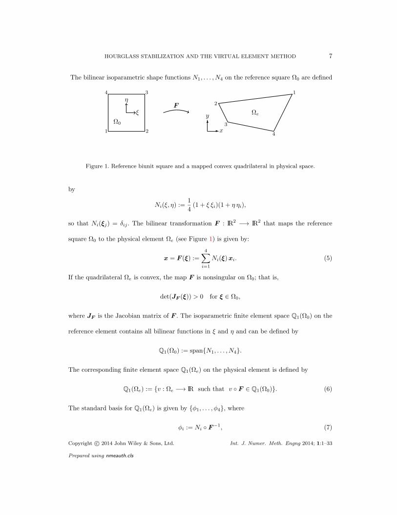
4.2. Hexahedral element
The definitions for the trilinear hexahedral element closely follow those indicated for the
bilinear quadrilateral element. The vertices of the hexahedral element Ωe in the physical
coordinate system are denoted by xi = (xi, yi, zi), i = 1, . . . , 8, and the reference cube is
Ω0 = (−1, 1)3. The vertices ξi = (ξi, ηi, ζi), i = 1, . . . , 8, in the reference cube are ordered as
follows:
ξ1 = (−1,−1,−1), ξ2 = (+1,−1,−1), ξ3 = (+1,+1,−1), ξ4 = (−1,+1,−1),
ξ5 = (−1,−1,+1), ξ6 = (+1,−1,+1), ξ7 = (+1,+1,+1), ξ8 = (−1,+1,+1).
The trilinear isoparametric shape functions N1, . . . , N8 on the reference cube Ω0 are defined
by
Ni(ξ, η, ζ) :=1
8(1 + ξ ξi)(1 + η ηi)(1 + ζ ζi),
so that Ni(ξj) = δij . The trilinear transformation F : IR3 −→ IR3 that maps the reference
cube Ω0 to the hexahedral element Ωe (see Figure 2) is given by:
x = F (ξ) :=
8∑
i=1
Ni(ξ)xi.
We assume that the map F is nonsingular on Ω0; that is,
det(JF (ξ)) > 0 for ξ ∈ Ω0.
Copyright c© 2014 John Wiley & Sons, Ltd. Int. J. Numer. Meth. Engng 2014; 1:1–33
Prepared using nmeauth.cls
HOURGLASS STABILIZATION AND THE VIRTUAL ELEMENT METHOD 9
1
2 3
4
5
6 7
8
ξη
ζ
Ω0
1
2
3
4
56
7
8
xy
z
Ωe
F
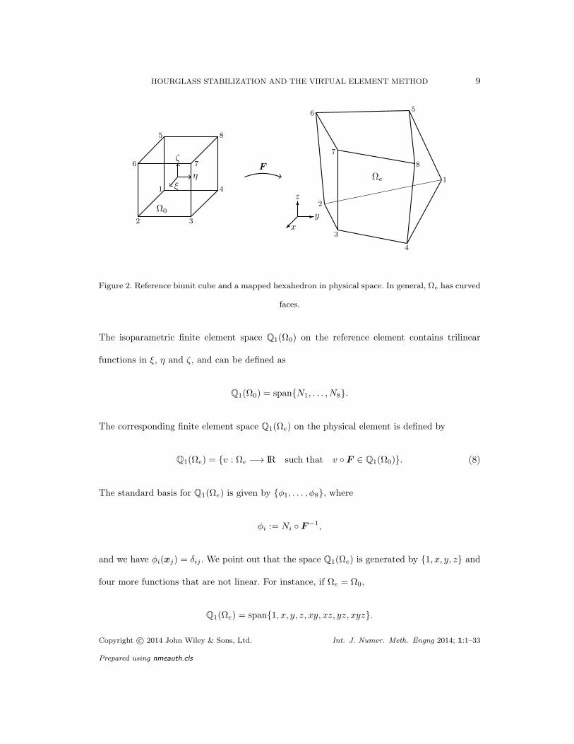
Figure 2. Reference biunit cube and a mapped hexahedron in physical space. In general, Ωe has curved
faces.
The isoparametric finite element space Q1(Ω0) on the reference element contains trilinear
functions in ξ, η and ζ, and can be defined as
Q1(Ω0) = spanN1, . . . , N8.
The corresponding finite element space Q1(Ωe) on the physical element is defined by
Q1(Ωe) = v : Ωe −→ IR such that v F ∈ Q1(Ω0). (8)
The standard basis for Q1(Ωe) is given by φ1, . . . , φ8, where
φi := Ni F−1,
and we have φi(xj) = δij . We point out that the space Q1(Ωe) is generated by 1, x, y, z and
four more functions that are not linear. For instance, if Ωe = Ω0,
Q1(Ωe) = span1, x, y, z, xy, xz, yz, xyz.
Copyright c© 2014 John Wiley & Sons, Ltd. Int. J. Numer. Meth. Engng 2014; 1:1–33
Prepared using nmeauth.cls

10 CANGIANI ET AL.
5. REDUCED INTEGRATION TECHNIQUES FOR THE POISSON PROBLEM
Now, we consider the isoparametric finite element approximation of problem (1). The domain
Ω is partitioned into a finite number of isoparametric elements Ωe, and let Q1(Ωe) be the
corresponding isoparametric finite element space introduced in the previous section. The
element stiffness matrix, is given by
Kij =
∫
Ωe
∇φi · ∇φj dx i, j = 1, . . . , 2d, (9)
which can be computed by mapping back to the reference element and then approximating
the integral with a quadrature formula. In Appendix A, we present the requirements on a
quadrature rule to meet the linear consistency property.
One-point quadrature approaches to compute the element stiffness matrix are based on the
simple approximation of (9) given by
|Ωe| ∇φi · ∇φj . (10)
Concerning the definition of ∇φi, there are a few options that are available. However, not all
choices maintain linear consistency that (10) is designed to achieve.
Irrespective of how a mean-gradient is defined, the element stiffness matrix K is the product
of two matrices each with rank d; hence, K has rank (at most) d and is rank-deficient. Because
the constant vector lies in the kernel of K, the correct rank of the element stiffness matrix is
3 for quadrilateral and 7 for hexahedral elements. The rank-deficiency of K allows spurious
singular modes to be present that can pollute the numerical solution. This deficiency is cured
by adding a correction term (stabilization matrix) to (10), and the various remedies for under-
integrated finite elements fall under the umbrella of what has come to be known as hourglass
control methods. In what follows, each method that we consider will be characterized by the
Copyright c© 2014 John Wiley & Sons, Ltd. Int. J. Numer. Meth. Engng 2014; 1:1–33
Prepared using nmeauth.cls

HOURGLASS STABILIZATION AND THE VIRTUAL ELEMENT METHOD 11
decomposition
K ≈ Kc +Ks,
where Kc is an instance of (10) (consistency term) and Ks is an hourglass correction (stability
term).
The mean-gradient approach of Flanagan and Belytschko [8] is based on defining
∇φi :=1
|Ωe|
∫
Ωe
∇φi dx. (11)
Following References [8, 10], we introduce the d× 2d matrix B whose columns are the mean-
gradients of the shape functions φi, and write B as
B =
bT
1
...
bT
d
, (12a)
where
bT
1 =1
|Ωe|
[∫
Ωe
∂φ1
∂xdx
∫
Ωe
∂φ2
∂xdx . . .
∫
Ωe
∂φ2d
∂xdx
], (12b)
and so on. With the above notation at hand, the consistency matrix due to Flanagan and
Belytschko [8] reads:
KFB
c:= |Ωe|
d∑
δ=1
bδbTδ . (13)
On observing that ∇p1 = ∇p1, because ∇p1 is a constant vector, we have
aFB
c (vh, p1) = |Ωe| ∇vh · ∇p1 =
(∫
Ωe
∇vh dx
)· ∇p1 =
∫
Ωe
∇vh · ∇p1 dx
= ae(vh, p1),
which shows that the approximate bilinear form corresponding to (13) is linearly consistent.
Another classical method, which is referred to as the Hallquist-approach [3, 17] is that of using
Copyright c© 2014 John Wiley & Sons, Ltd. Int. J. Numer. Meth. Engng 2014; 1:1–33
Prepared using nmeauth.cls

12 CANGIANI ET AL.
the one-point Gauss quadrature for ∇φi; that is,
∇φi := ∇φi(x), (14)
where x := 12d
∑2d
i=1 xi is the centroid of the vertices of Ωe. In two dimensions, the mean-
gradient formula and the one-point Gauss formula coincide; that is,
1
|Ωe|
∫
Ωe
∇φi dx = ∇φi(x) (d = 2 only). (15)
A proof of this fact is given in Section 8. On the other hand, for a hexahedral element
the mean-gradient and the gradient obtained via the one-point Gauss rule do not coincide,
and employing (14) does not lead to a linearly consistent scheme, which was recognized in
Reference [8]. We now discuss the hourglass control method of Flanagan and Belytschko [8].
The two- and three-dimensional cases are treated separately, and we begin with the two-
dimensional case.
5.1. Two-dimensional case
For d = 2, there is one hourglass vector, namely
Γ =
[+1 −1 +1 −1
]T, (16)
such that KFB
cΓ = 0. In what follows, we shall also make use of the vectors
s :=
[+1 +1 +1 +1
]T, X :=
[x1 x2 x3 x4
]T, Y :=
[y1 y2 y3 y4
]T, (17)
which are associated with the linear polynomial basis 1, x, y. Direct verification yields the
orthogonality relations:
sTΓ = 0, bTδ s = 0, bTδ Γ = 0 for δ = 1, 2,
Copyright c© 2014 John Wiley & Sons, Ltd. Int. J. Numer. Meth. Engng 2014; 1:1–33
Prepared using nmeauth.cls

HOURGLASS STABILIZATION AND THE VIRTUAL ELEMENT METHOD 13
so that every vector γ ∈ IR4 can be expanded as γ = a1b1 + a2b2 + a3s + a4Γ. Because
bT
1X = bT
2Y = 1 and bT
1Y = bT
2X = 0, imposing orthogonality of γ with respect to the affine
basis in (17) yields the one-dimensional vector space spanned by the vector [8, 10]:
γ = Γ− (ΓTX)b1 − (ΓTY )b2. (18)
The vector γ resulting from (18) is explicitly given by Flanagan and Belytschko [8, p. 690]:
γ =1
4|Ωe|
x2(y3 − y4) + x3(y4 − y2) + x4(y2 − y3)
x3(y1 − y4) + x4(y3 − y1) + x1(y4 − y3)
x4(y1 − y2) + x1(y2 − y4) + x2(y4 − y1)
x1(y3 − y2) + x2(y1 − y3) + x3(y2 − y1)
. (19)
We can now define the stability term:
KFB
s:= |Ωe| ǫγγ
T (d = 2), (20)
with ǫ ∈ IR being a parameter that reflects the freedom of choice for the vector γ. In order to
ensure convergence, the parameter ǫ must be correctly scaled (ǫ = O(h−2e ) when d = 2). This
fact is clearly established via the VEM in Section 7.
By construction, KFB
sv = 0 whenever v represents an affine field, that is, a linear
combination of the vectors defined in (17), thus ensuring that the method given by
KFB := KFB
c+KFB
s(21)
is linearly consistent. In addition, KFB has the correct rank, thus excluding the presence of
spurious singular modes. Hence, by Theorem 1 the corresponding method passes the patch
test.
Copyright c© 2014 John Wiley & Sons, Ltd. Int. J. Numer. Meth. Engng 2014; 1:1–33
Prepared using nmeauth.cls

14 CANGIANI ET AL.
5.2. Three-dimensional case
For d = 3, we proceed as in the d = 2 case. Here, the spurious modes are related to the four
vectors [8]
Γ1 =
[+1 +1 −1 −1 −1 −1 +1 +1
]T, Γ2 =
[+1 −1 −1 +1 −1 +1 +1 −1
]T,
Γ3 =
[+1 −1 +1 −1 +1 −1 +1 −1
]T, Γ4 =
[−1 +1 −1 +1 +1 −1 +1 −1
]T,
(22)
which represent the hourglass modes of the reference element. In analogy with the two-
dimensional case, we define the vectors:
s :=
[+1 +1 +1 +1 +1 +1 +1 +1
]T, X :=
[x1 x2 x3 x4 x5 x6 x7 x8
]T,
Y :=
[y1 y2 y3 y4 y5 y6 y7 y8
]T, Z :=
[z1 z2 z3 z4 z5 z6 z7 z8
]T.
(23)
Flanagan and Belytschko [8] infer that the eight vectors Γα, bδ, and s are linearly independent
and form a basis for IR8, and hence consider the following four vectors γα ∈ IR8:
γα := aαs+
3∑
δ=1
aαδbδ +
4∑
β=1
aαβΓβ , α = 1, . . . , 4
that are mutually linearly independent and orthogonal to all vectors associated with affine
fields. On imposing orthogonality with affine fields, the four basis vectors are obtained:
γα = Γα − (ΓT
αX) b1 − (ΓT
αY ) b2 − (ΓT
αZ) b3, α = 1, . . . , 4. (24)
Since each of the vectors γα is a linear combination of just one of the hourglass vectors and
the three bδ vectors, and all these vectors are linearly independent, it follows that the γα are
linearly independent as required. Hence,
KFB
s:= |Ωe|
4∑
α=1
ǫαγαγT
α (d = 3), (25)
Copyright c© 2014 John Wiley & Sons, Ltd. Int. J. Numer. Meth. Engng 2014; 1:1–33
Prepared using nmeauth.cls

HOURGLASS STABILIZATION AND THE VIRTUAL ELEMENT METHOD 15
and ǫα := ǫ ∈ IR (free parameter) for all α is the choice made in Reference [8]. Finally, the
element stiffness matrix KFB can be constructed as in (21):
KFB := KFB
c+KFB
s= |Ωe|
(3∑
i=1
bibT
i + ǫ
4∑
α=1
γαγT
α
), (26)
which leads to a linearly consistent and stable method that passes the patch test.
6. VIRTUAL ELEMENT FRAMEWORK
The virtual element method is a general framework for devising consistent and stable Galerkin
approximations in the sense of Section 3.1. We assume that the space V Eh contains linear
polynomials and other functions that are not linear. The key steps of the VEM are as follows:
• a definition of the space V Eh and vertex degrees of freedom that are associated with the
Lagrange shape functions φ1, . . . , φnE.
• the construction of a projector
Π∇E : V E
h −→ P1(E), (27)
which is orthogonal with respect to the aE(·, ·) scalar product that is induced by
problem (1).
• the exact decomposition of the local stiffness matrix (9) as the sum of a computable
consistency matrix Kvem
cand an uncomputable stability matrix K∗
sas
KE = Kvem
c+K∗
s, (28a)
with
(Kvem
c)ij :=
∫
E
∇Π∇Eφi · ∇Π∇
Eφj dx, (28b)
(K∗s)ij :=
∫
E
∇(I−Π∇E )φi · ∇(I−Π∇
E )φj dx. (28c)
Copyright c© 2014 John Wiley & Sons, Ltd. Int. J. Numer. Meth. Engng 2014; 1:1–33
Prepared using nmeauth.cls

16 CANGIANI ET AL.
• the replacement of the exact stability matrix K∗s
with the inexact but computable
matrix Kvem
syields the final virtual element decomposition of the stiffness matrix:
Kvem := Kvem
c+Kvem
s, (29)
with Kvem
sdefined by
(Kvem
s)ij :=
nE∑
k,l=1
(δik − s
(i)k
)Skl
(δjl − s
(j)l
), (30)
where δik is the Kronecker-delta symbol, Skl are the elements of S, a symmetric matrix
whose construction is presented in Section 8.2, and s(i)k are the coefficients of Π∇
Eφi in
terms of the φk:
Π∇Eφi =
nE∑
k=1
s(i)k φk. (31)
6.1. Definition of the projector Π∇E
The element-wise projector Π∇E clearly separates the consistency term from the stability term.
It is defined as a Ritz-like projection operator that maps functions defined on E to linear
polynomials. Given a function v defined on E, the projection Π∇Ev ∈ P1(E) of v is defined by
requiring that v −Π∇Ev is aE-orthogonal to all linear polynomials:
aE(v −Π∇Ev, p1) = 0 for all p1 ∈ P1(E). (32)
Because aE(·, 1) is identically zero, (32) defines Π∇Ev only up to a constant. To complete the
definition of Π∇E , we need another ingredient: a projection operator P0 onto the kernel of
aE(·, ·), that is, the space of constant functions, and we require that
P0(v −Π∇Ev) = 0. (33)
Copyright c© 2014 John Wiley & Sons, Ltd. Int. J. Numer. Meth. Engng 2014; 1:1–33
Prepared using nmeauth.cls

HOURGLASS STABILIZATION AND THE VIRTUAL ELEMENT METHOD 17
For the first-order VEM considered in this paper, the projection P0v is defined as the mean-
value of v over the nE vertices of E [18]:
P0v := v =1
nE
nE∑
i=1
v(xi). (34)
On writing (32) explicitly, we obtain
∫
E
∇Π∇Ev · ∇p1 dx =
∫
E
∇v · ∇p1 dx, (35)
and because ∇Π∇Ev and ∇p1 are constant vectors, (35) becomes
∇Π∇Ev · ∇p1 |E| = ∇p1 ·
∫
E
∇v dx. (36)
On choosing p1 = x and p1 = y, we find that (36) is equivalent to
∇Π∇Ev =
1
|E|
∫
E
∇v dx. (37)
Equation (37) determines Π∇Ev up to a constant:
Π∇Ev = x ·
1
|E|
∫
E
∇v dx+ C. (38)
The constant C is fixed by applying the projection P0 to both sides of (38), which yields
Π∇Ev = (x− P0x) ·
1
|E|
∫
E
∇v dx+ P0v.
On noting that
P0x =1
nE
nE∑
i=1
xi =: x (39)
is the centroid of the set of nodes x1, . . . ,xnE and using the definition of P0v, we arrive at
the following explicit formula for the Π∇E projection:
Π∇Ev = (x− x) ·
1
|E|
∫
E
∇v dx+ v. (40)
Copyright c© 2014 John Wiley & Sons, Ltd. Int. J. Numer. Meth. Engng 2014; 1:1–33
Prepared using nmeauth.cls

18 CANGIANI ET AL.
Remark 1. The projection Π∇Ev is fully determined by knowing v on ∂E:
∫
E
∇v dx =
∫
∂E
vn ds. (41)
When d = 2 and v is piecewise linear on the edges of the polygon, the integral on the right-hand
side of (41) is exactly computed through the trapezoidal rule. This requires only knowing the
values of v at the vertices of E.
7. POLYGONAL AND POLYHEDRAL VIRTUAL ELEMENT METHOD
In this section, we recall the first-order virtual element method for polygonal and polyhedral
meshes. For a complete description of the theory and implementation of arbitrary-order
VEM, we refer the interested reader to References [16, 18–20]. The connection with mimetic
discretizations [21] is discussed in Reference [22].
7.1. Definition of the space V Eh for d = 2
In two dimensions, a function vh ∈ V Eh is characterized by the following properties:
• vh is continuous and piecewise linear on the polygonal boundary ∂E
• ∆vh is a linear polynomial
•
∫
E
vh p1 dx =
∫
E
Π∇Evh p1 dx for all linear polynomials p1.
(42)
Note that the second condition is distinct from the one introduced in Reference [16] (∆vh = 0).
In addition, the third condition states that Π∇Evh is also the L2-projection of vh onto linear
polynomials [23]. These two modifications are adopted to enable the computation in 3D to be
performed using only the values of vh at the vertices of E. The dimension of V Eh is equal to
nE , the number of vertices of E, and the values of vh at these vertices are taken as the degrees
Copyright c© 2014 John Wiley & Sons, Ltd. Int. J. Numer. Meth. Engng 2014; 1:1–33
Prepared using nmeauth.cls

HOURGLASS STABILIZATION AND THE VIRTUAL ELEMENT METHOD 19
of freedom. Due to Remark 1, we are able to compute Π∇Evh exactly.
7.2. Definition of the space V Eh for d = 3
In three dimensions, a function vh ∈ V Eh is characterized by the following properties:
• the restriction of vh to a face f belongs to V f
h as defined in (42)
• ∆vh is a linear polynomial
•
∫
E
vh p1 dx =
∫
E
Π∇Evh p1 dx for all linear polynomials p1.
(43)
The dimension of V Eh is equal to nE and we take the values of vh at the vertices as degrees of
freedom. The first property in (43) implies that vh is linear on each edge of E and its trace on
f is uniquely determined by the values at the vertices of f. Consequently, vh is also continuous
on ∂E . If vh ∈ V Eh , we can still compute Π∇
Evh using only the vertex values of vh. Indeed, a
face f of E is a polygon; hence, we can define on f the projector Π∇f
and the space V f
h as in
(42). From (40), we only need to compute the mean value of ∇vh and can write
∫
E
∇vh dx =
∫
∂E
vh n ds =∑
f⊂∂E
nf
∫
f
vh ds =∑
f⊂∂E
nf
∫
f
Π∇fvh ds, (44)
where the third relation in (42) with p1 = 1 is used to obtain the last equality.
7.3. Stiffness matrix of the VEM
We assume that the degrees of freedom of a function vh ∈ V Eh are the pointwise values of vh
at the nodes xi of the element E; that is,
dofi(vh) = vh(xi). (45)
Remark 2. Let dofi(vh) be the i-th degree of freedom of vh defined on some fixed element
and dofi(vh) the value of the corresponding degree of freedom on a rescaled element. If
Copyright c© 2014 John Wiley & Sons, Ltd. Int. J. Numer. Meth. Engng 2014; 1:1–33
Prepared using nmeauth.cls

20 CANGIANI ET AL.
dofi(vh) = dofi(vh) for all i, then the degrees of freedom are scale invariant. This property is
trivially met if the degrees of freedom are pointwise values of vh.
The Lagrange shape functions associated with the vertex degrees of freedom are given by
φ1, . . . , φnE, where φi ∈ V E
h is identified by the following property:
φi(xj) = δij ,
which leads to the following representation of functions vh ∈ V Eh :
vh(x) =
nE∑
i=1
vh(xi)φi(x).
We now consider the decomposition Kvem = Kvem
c+Kvem
sgiven in (29) with the consistency
matrix Kvem
cand stability matrix Kvem
sdefined by (28b) and (30), respectively. On using (37),
we rewrite the consistency term as follows:
(Kvem
c)ij =
∫
E
∇Π∇Eφi · ∇Π∇
Eφj dx =
∫
E
(1
|E|
∫
E
∇φi dx
)·
(1
|E|
∫
E
∇φj dx
)dx
= |E|
(1
|E|
∫
E
∇φi dx
)·
(1
|E|
∫
E
∇φj dx
)=
1
|E|
∫
E
∇φi dx ·
∫
E
∇φj dx. (46)
The VEM stability term Kvem
sreplacing K∗
sis constructed as follows:
1. Because Π∇Eφi belongs to P1(E), which is a subspace of V E
h , Π∇Eφi can in turn be written
in terms of the φk’s:
Π∇Eφi =
nE∑
k=1
s(i)k φk, (I−Π∇
E )φi =
nE∑
k=1
(δik − s(i)k )φk. (47)
From (45), we have
Π∇Eφi =
nE∑
k=1
(Π∇Eφi)(xk)φk and φi =
1
nE
nE∑
j=1
φi(xj) =1
nE,
and therefore s(i)k defined in (47) is given by
s(i)k = dofk(Π
∇Eφi) = (Π∇
Eφi)(xk) = (xk − x) ·1
|E|
∫
E
∇φi dx+1
nE.
Copyright c© 2014 John Wiley & Sons, Ltd. Int. J. Numer. Meth. Engng 2014; 1:1–33
Prepared using nmeauth.cls
HOURGLASS STABILIZATION AND THE VIRTUAL ELEMENT METHOD 21
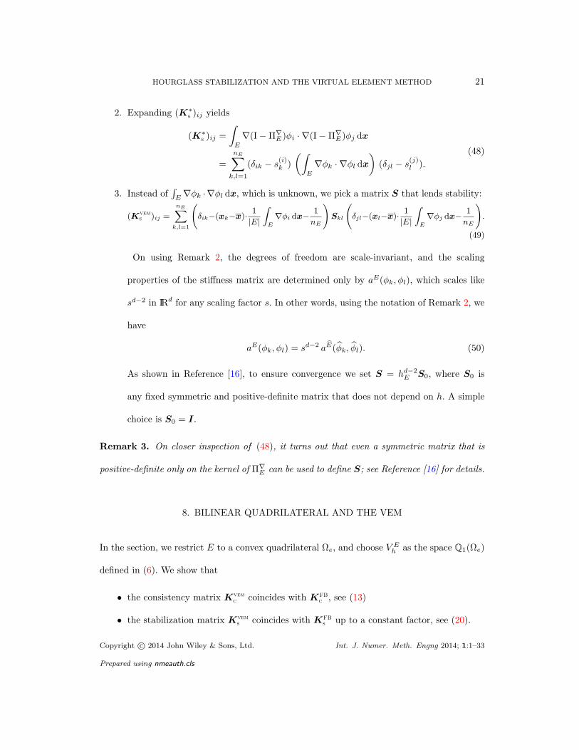
2. Expanding (K∗s)ij yields
(K∗s)ij =
∫
E
∇(I−Π∇E )φi · ∇(I−Π∇
E )φj dx
=
nE∑
k,l=1
(δik − s(i)k )
(∫
E
∇φk · ∇φl dx
)(δjl − s
(j)l ).
(48)
3. Instead of∫E∇φk ·∇φl dx, which is unknown, we pick a matrix S that lends stability:
(Kvem
s )ij =
nE∑
k,l=1
(
δik−(xk−x)·1
|E|
∫
E
∇φi dx−1
nE
)
Skl
(
δjl−(xl−x)·1
|E|
∫
E
∇φj dx−1
nE
)
.
(49)
On using Remark 2, the degrees of freedom are scale-invariant, and the scaling
properties of the stiffness matrix are determined only by aE(φk, φl), which scales like
sd−2 in IRd for any scaling factor s. In other words, using the notation of Remark 2, we
have
aE(φk, φl) = sd−2 aE(φk, φl). (50)
As shown in Reference [16], to ensure convergence we set S = hd−2E S0, where S0 is
any fixed symmetric and positive-definite matrix that does not depend on h. A simple
choice is S0 = I.
Remark 3. On closer inspection of (48), it turns out that even a symmetric matrix that is
positive-definite only on the kernel of Π∇E can be used to define S; see Reference [16] for details.
8. BILINEAR QUADRILATERAL AND THE VEM
In the section, we restrict E to a convex quadrilateral Ωe, and choose V Eh as the space Q1(Ωe)
defined in (6). We show that
• the consistency matrix Kvem
ccoincides with KFB
c, see (13)
• the stabilization matrix Kvem
scoincides with KFB
sup to a constant factor, see (20).
Copyright c© 2014 John Wiley & Sons, Ltd. Int. J. Numer. Meth. Engng 2014; 1:1–33
Prepared using nmeauth.cls

22 CANGIANI ET AL.
8.1. Consistency matrix
The consistency matrix Kvem
cis given by (46):
(Kvem
c)ij =
1
|Ωe|
∫
Ωe
∇φi dx ·
∫
Ωe
∇φj dx. (51)
From the definitions in (12a) and (12b) for the vectors bδ, it is observed that
|Ωe| (b1bT
1 )ij =1
|Ωe|
∫
Ωe
∂φi
∂xdx
∫
Ωe
∂φj
∂xdx,
so that
(KFB
c)ij = |Ωe|
2∑
δ=1
(bδbTδ )ij =
1
|Ωe|
∫
Ωe
∇φi dx ·
∫
Ωe
∇φj dx = (Kvem
c)ij .
We first prove that the consistency matrix Kvem
cgiven in (51) is identical to that obtained
by applying one-point Gauss quadrature rule to the exact stiffness matrix∫Ωe
∇φi · ∇φj dx.
To this end, we begin by showing the equivalence stated in (15), namely that if vh ∈ Q1(Ωe),
then approximating ∇vh by its value at the vertex center x of Ωe is equivalent to taking its
mean-value over Ωe, where x is defined in (39). It suffices to show the equality for a particular
basis of Q1(Ωe); we choose the basis set 1, x, y,Ψ where Ψ is the (unique) function in Q1(Ωe)
such that
Ψ(x1) = −1/2, Ψ(x2) = +1/2, Ψ(x3) = −1/2, Ψ(x4) = +1/2. (52)
The function Ψ on the reference biunit square is shown in Figure 3. It is noted that 1, x, y,Ψ
is indeed a basis of Q1(Ωe). For vh = 1, x, or y the equality is evident because the gradient is
constant; for vh = Ψ, both terms are zero:
• the left-hand side of (15) is zero because the integral of Ψ on each edge is zero; and
• the right-hand side of (15) is zero because Ψ is zero at the midpoint of each edge, and
hence it is identically zero along the two bimedians of Ωe that meet precisely at x.
Copyright c© 2014 John Wiley & Sons, Ltd. Int. J. Numer. Meth. Engng 2014; 1:1–33
Prepared using nmeauth.cls

HOURGLASS STABILIZATION AND THE VIRTUAL ELEMENT METHOD 23
Figure 3. The function Ψ(ξ) =ξη
2on the reference biunit square.
Now, the consistency matrix Kvem
ccan be written as
(Kvem
c)ij =
1
|Ωe|
∫
Ωe
∇φi dx ·
∫
Ωe
∇φj dx = |Ωe| ∇φi(x) · ∇φj(x),
which is equal to
|Ωe|J−TF (0, 0)∇ξNi(0, 0) · J
−TF (0, 0)∇ξNj(0, 0), (53)
because (0, 0) is mapped to x in the bilinear transformation F that maps the reference square
Ω0 = (−1, 1)2 to the convex quadrilateral Ωe.
We now establish that detJF (0, 0) = |Ωe|/|Ω0|. Because detJF (ξ, η) is bilinear in ξ and η,
the one-point Gauss quadrature rule on Ω0 integrates it exactly:
|Ωe| =
∫
Ω0
detJF (ξ, η) dξ = |Ω0| detJF (0, 0). (54)
On substituting expression (54) into (53), we obtain
(Kvem
c)ij = |Ω0|J
−TF (0, 0)∇ξNi(0, 0) · J
−TF (0, 0)∇ξNj(0, 0) detJF (0, 0),
Copyright c© 2014 John Wiley & Sons, Ltd. Int. J. Numer. Meth. Engng 2014; 1:1–33
Prepared using nmeauth.cls

24 CANGIANI ET AL.
which is precisely the one-point Gauss quadrature formula applied to∫Ωe
∇φi · ∇φj dx.
We can express Kvem
cdirectly in terms of the vertex coordinates of the quadrilateral. On
invoking the divergence theorem, we have
∫
Ωe
∇φi dx =
∫
∂Ωe
φin ds =4∑
k=1
(∫
ek
φi ds
)nk
=
(∫
ei−1
φi ds
)ni−1 +
(∫
ei
φi ds
)ni =
|ei−1|
2ni−1 +
|ei|
2ni,
because φi is an affine function on each edge ek of the quadrilateral Ωe. Letting di be the
vector joining vertex xi−1 to xi+1, we have
|ei−1|
2ni−1 +
|ei|
2ni =
1
2d⊥i ,
where ⊥ refers to a clockwise rotation of 90. Hence,
(Kvem
c)ij :=
1
4|Ωe|d⊥i · d⊥
j =1
4|Ωe|di · dj .
For a convex quadrilateral, we have
d3 = −d1, d4 = −d2,
and therefore the matrix Kvem
chas the block structure
Kvem
c=
+U −U
−U +U
, where U =
1
4|Ωe|
d1 · d1 d1 · d2
d1 · d2 d2 · d2
. (55)
8.2. Stabilization matrix
Instead of starting from (49), we compute the stabilization matrix Kvem
sas follows. Because
there is only one nonlinear function in Q1(Ωe), we can explicitly compute the expansion of
(I − Π∇E )φi in terms of the basis functions φk; that is, we directly compute the coefficients
(δik − s(i)k ) of (47).
Copyright c© 2014 John Wiley & Sons, Ltd. Int. J. Numer. Meth. Engng 2014; 1:1–33
Prepared using nmeauth.cls

HOURGLASS STABILIZATION AND THE VIRTUAL ELEMENT METHOD 25
We start by finding a function in the kernel of the Π∇E operator, that is, a zero-energy mode.
A candidate is the function Ψ in (52), which corresponds to the vector Γ in (16). From the
definition of Ψ, we have
Ψ =1
2(−φ1 + φ2 − φ3 + φ4) =
1
2
4∑
k=1
(−1)kφk.
Let us show that the function Ψ is a zero-energy mode; that is, Π∇EΨ = 0. From (40), we have
Π∇EΨ = (x− x) ·
1
|Ωe|
∫
Ωe
∇Ψdx+Ψ.
From the divergence theorem, it follows that
∫
Ωe
∇Ψdx =
∫
∂Ωe
Ψn ds =4∑
k=1
(∫
ek
Ψds
)nk = 0,
because Ψ has zero mean-value on each edge. Since Ψ = 0, it follows that Π∇EΨ = 0.
Furthermore, (45) implies that
1 =
4∑
i=1
φi, x =
4∑
i=1
xiφi and y =
4∑
i=1
yiφi.
Therefore, the linear transformation from the basis φ1, φ2, φ3, φ4 to the basis 1, x, y,Ψ of
Q1(Ωe) is:
1 1 1 1
x1 x2 x3 x4
y1 y2 y3 y4
−1/2 +1/2 −1/2 +1/2
φ1
φ2
φ3
φ4
=
1
x
y
Ψ
. (56)
Let us denote by Ti the signed area of the triangle obtained by removing the vertex xi from
Copyright c© 2014 John Wiley & Sons, Ltd. Int. J. Numer. Meth. Engng 2014; 1:1–33
Prepared using nmeauth.cls

26 CANGIANI ET AL.
the quadrilateral Ωe. Therefore,
T1 :=1
2det
1 1 1
x2 x3 x4
y2 y3 y4
, T2 :=
1
2det
1 1 1
x1 x3 x4
y1 y3 y4
,
T3 :=1
2det
1 1 1
x1 x2 x4
y1 y2 y4
, T4 :=
1
2det
1 1 1
x1 x2 x3
y1 y2 y3
.
Now, let us consider the coefficient matrix of the linear system in (56). Carrying out the
expansion with respect to the last row, it is verified that its determinant is equal to 2|Ωe|. By
directly solving system (56) through the Cramer’s rule, we see that
φ1 =
det
1 1 1 1
x x2 x3 x4
y y2 y3 y4
Ψ +1/2 −1/2 +1/2
2 |Ωe|= (a1 + b1x+ c1y)−
2T1
2|Ωe|Ψ,
and in general one can write
φi = (ai + bix+ ciy) + (−1)iTi
|Ωe|Ψ, i = 1, . . . , 4,
where the coefficients ai, bi, ci depend on the coordinates of the vertices. Since Π∇EΨ = 0, we
have Π∇Eφi = ai + bix+ ciy, so that
(I−Π∇E )φi = (−1)i
Ti
|Ωe|Ψ = (−1)i
Ti
|Ωe|
(1
2
4∑
k=1
(−1)kφk
),
that is,
δik − s(i)k = (−1)i+k Ti
2|Ωe|.
Copyright c© 2014 John Wiley & Sons, Ltd. Int. J. Numer. Meth. Engng 2014; 1:1–33
Prepared using nmeauth.cls

HOURGLASS STABILIZATION AND THE VIRTUAL ELEMENT METHOD 27
Hence, the stabilization matrix Kvem
sis written as
(Kvem
s)ij =
4∑
k,l=1
(δik − s
(i)k
)Skl
(δjl − s
(j)l
)
=4∑
k,l=1
((−1)i+k Ti
2|Ωe|
)Skl
((−1)j+l Tj
2|Ωe|
)
= (−1)i+j Ti Tj
|Ωe|2
1
4
4∑
k,l=1
(−1)k+lSkl
.
(57)
Since d = 2, we let S = I in (57) and obtain
(Kvem
s)ij = (−1)i+j Ti Tj
|Ωe|2. (58)
On defining the nondimensional quantities T ′i = Ti/|Ωe|, and setting
γ :=
[+T ′
1 −T ′2 +T ′
3 −T ′4
]T, (59)
the matrix in (58) is written as
Kvem
s= γγT. (60)
The Flanagan-Belytschko vector γ in (19) is equal to the VEM vector γ defined in (59) divided
by 2; hence
KFB
s=
|Ωe| ǫ
4Kvem
s.
If τ is a positive parameter independent of the mesh, the stiffness matrix of the VEM for
S = τI is given by [16]
Kvem = Kvem
c+ τγγT, (61)
which always results in a scheme that is convergent. Hence, in order to yield a convergent
scheme, the parameter ǫ that appears in the Flanagan-Belytschko stabilization matrix must
scale like h−2e .
Copyright c© 2014 John Wiley & Sons, Ltd. Int. J. Numer. Meth. Engng 2014; 1:1–33
Prepared using nmeauth.cls

28 CANGIANI ET AL.
Remark 4. When Ωe is a parallelogram, we have
γ =1
2
[+1 −1 +1 −1
]T,
and
γγT =1
4
+1 −1 +1 −1
−1 +1 −1 +1
+1 −1 +1 −1
−1 +1 −1 +1
, (62)
which when scaled by a factor of 2 coincides with the hourglass control matrix of Hansbo [24].
Remark 5. Taking S = τI corresponds to approximating the energy of function Ψ with τ :
∫
Ωe
|∇Ψ|2 dx =
nE∑
k,l=1
(−1)k+l
4
∫
Ωe
∇φk · ∇φl dx ≈
nE∑
k,l=1
(−1)k+l
4τ δkl = τ.
In general, we have∫
Ωe
|∇Ψ|2 dx =
∫
Ω0
|J−TF ∇ξΨ|2 det(JF ) dξ,
which usually can not be integrated in closed-form. The following identity holds for the exact
stiffness matrix K for any quadrilateral Ωe:
K = Kvem
c+
[∫
Ωe
|∇Ψ|2 dx
]γγT, (63)
where Kvem
cand γ are defined in (51) and (59), respectively. Because
Ψ =1
2(−φ1 + φ2 − φ3 + φ4) and φ1 + φ2 + φ3 + φ4 = 1,
we have
Ψ =1
2− φ1 − φ3 =
1
2+ φ2 + φ4,
so that∫
Ωe
|∇Ψ|2 dx =
∫
Ωe
|∇(φ1 + φ3)|2 dx =
∫
Ωe
|∇(φ2 + φ4)|2 dx.
Copyright c© 2014 John Wiley & Sons, Ltd. Int. J. Numer. Meth. Engng 2014; 1:1–33
Prepared using nmeauth.cls

HOURGLASS STABILIZATION AND THE VIRTUAL ELEMENT METHOD 29
In Appendix B.1, on using τ as a parameter, the stencils that are obtained from the VEM for a
uniform square grid are compared to well-known finite-difference stencils, whereas in Appendix
B.2 we exploit the VEM decomposition (63) for a few special quadrilaterals.
9. TRILINEAR HEXAHEDRON AND THE VEM
We now consider the case when E is a hexahedron Ωe and V Eh is the space Q1(Ωe) defined
in (8). We show that
• the consistency matrix Kvem
ccoincides with that obtained via reduced integration
(mean-gradient formulation) of the exact bilinear form.
• The stabilization matrix Kvem
scoincides with the Flanagan-Belytschko stabilization of
the hourglass modes for a particular choice of the matrix S.
9.1. Consistency matrix
The consistency matrix Kvem
cis given by (46):
(Kvem
c)ij =
1
|Ωe|
∫
Ωe
∇φi dx ·
∫
Ωe
∇φj dx. (64)
Following the same arguments as in Section 8, we conclude that
Kvem
c= KFB
c,
that is, the VEM consistency matrix (64) and the Flanagan-Belytschko consistency matrix (13)
coincide.
As already noted, for the eight-node hexahedral isoparametric element, use of the one-point
Gauss quadrature to integrate ∇φi is not equivalent to taking the mean-value of ∇φi over the
element. In other words, (15) does not hold in three dimensions. The integral of the gradient
Copyright c© 2014 John Wiley & Sons, Ltd. Int. J. Numer. Meth. Engng 2014; 1:1–33
Prepared using nmeauth.cls

30 CANGIANI ET AL.
of the basis functions can be explicitly computed by mapping back to the reference element
Ω0 [8]:
∫
Ωe
∇φi dx =
∫
Ω0
J−TF ∇ξNi det(JF ) dξ. (65)
Equation (65) — when combined with (46) and (49) — permits the virtual element
decomposition to be applicable to hexahedral elements with curved faces that are the image
in the physical space of the reference biunit cube.
9.2. Stabilization matrix
Using (49), we take S = heI and obtain a convergent virtual element method, which is
confirmed by our numerical experiments in Section 10. To draw comparisons between the
stabilization matrices Kvem
sand KFB
s, we need to discuss the conditions on the matrix S. As
pointed out in Remark 3, matrix S need not be symmetric and strictly positive-definite; it
can just be positive-definite on the linear subspace of vectors representing the kernel of Π∇E ,
which corresponds to the nonpolynomial functions. Hence, the kernel of S can include the
vectors representing polynomial functions, and in particular, all constant functions, which are
polynomials of degree zero. If so, then (49) simplifies to
(Kvem
s)ij =
8∑
k,l=1
(δik − xk ·
1
|E|
∫
E
∇φi dx)Skl
(δjl − xl ·
1
|E|
∫
E
∇φj dx), (66)
where we have left out the terms that do not depend on the indices k and l; because the
constant lies in the kernel of S, the omitted terms do not contribute to Kvem
s.
Now, we are ready to show that the Flanagan-Belytschko stabilization matrix KFB
sis equal
Copyright c© 2014 John Wiley & Sons, Ltd. Int. J. Numer. Meth. Engng 2014; 1:1–33
Prepared using nmeauth.cls
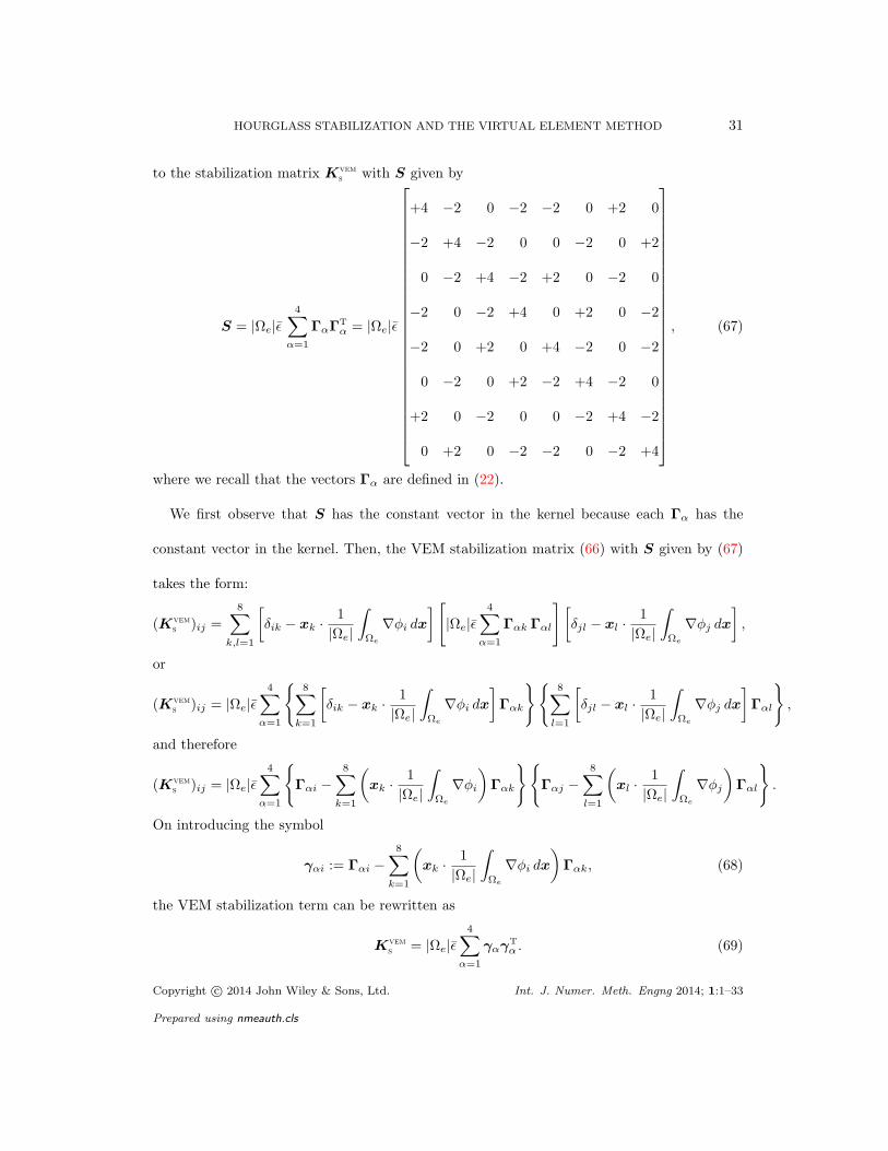
HOURGLASS STABILIZATION AND THE VIRTUAL ELEMENT METHOD 31
to the stabilization matrix Kvem
swith S given by
S = |Ωe|ǫ4∑
α=1
ΓαΓT
α = |Ωe|ǫ
+4 −2 0 −2 −2 0 +2 0
−2 +4 −2 0 0 −2 0 +2
0 −2 +4 −2 +2 0 −2 0
−2 0 −2 +4 0 +2 0 −2
−2 0 +2 0 +4 −2 0 −2
0 −2 0 +2 −2 +4 −2 0
+2 0 −2 0 0 −2 +4 −2
0 +2 0 −2 −2 0 −2 +4
, (67)
where we recall that the vectors Γα are defined in (22).
We first observe that S has the constant vector in the kernel because each Γα has the
constant vector in the kernel. Then, the VEM stabilization matrix (66) with S given by (67)
takes the form:
(Kvem
s)ij =
8∑
k,l=1
[δik − xk ·
1
|Ωe|
∫
Ωe
∇φi dx
] [|Ωe|ǫ
4∑
α=1
Γαk Γαl
] [δjl − xl ·
1
|Ωe|
∫
Ωe
∇φj dx
],
or
(Kvem
s)ij = |Ωe|ǫ
4∑
α=1
8∑
k=1
[δik − xk ·
1
|Ωe|
∫
Ωe
∇φi dx
]Γαk
8∑
l=1
[δjl − xl ·
1
|Ωe|
∫
Ωe
∇φj dx
]Γαl
,
and therefore
(Kvem
s)ij = |Ωe|ǫ
4∑
α=1
Γαi −
8∑
k=1
(xk ·
1
|Ωe|
∫
Ωe
∇φi
)Γαk
Γαj −
8∑
l=1
(xl ·
1
|Ωe|
∫
Ωe
∇φj
)Γαl
.
On introducing the symbol
γαi := Γαi −8∑
k=1
(xk ·
1
|Ωe|
∫
Ωe
∇φi dx
)Γαk, (68)
the VEM stabilization term can be rewritten as
Kvem
s= |Ωe|ǫ
4∑
α=1
γαγT
α . (69)
Copyright c© 2014 John Wiley & Sons, Ltd. Int. J. Numer. Meth. Engng 2014; 1:1–33
Prepared using nmeauth.cls

32 CANGIANI ET AL.
Comparing the previous equality to (25), we only have to check that γ defined in (24) is equal
to γ defined in (68). Because
[(ΓT
αX) b1]i =
(8∑
k=1
Γαkxk
)1
|Ωe|
∫
Ωe
∂φi
∂xdx =
8∑
k=1
(xk
1
|Ωe|
∫
Ωe
∂φi
∂xdx
)Γαk,
we have
[Γα − (ΓT
αX) b1 − (ΓT
αY ) b2 − (ΓT
αZ) b3]i = Γαi −
8∑
k=1
(xk ·
1
|Ωe|
∫
Ωe
∇φi
)Γαk,
so that (24) and (68) coincide. We conclude that KFB
s= Kvem
sfor S given by (67) and that
optimal convergence is ensured if the parameter ǫ of (69) scales like h−2e [16]. This fact is
confirmed by the numerical experiments presented in Section 10. Furthermore, we need to
check that matrix S is positive-definite on the linear subspace of V Eh that represents the
kernel of Π∇E , that is, the nonlinear functions. To this end, it suffices to show that in the kernel
of S there are no vectors of V Eh corresponding to the nonlinear functions, and this is precisely
what has been shown in Reference [25].
10. NUMERICAL EXAMPLES
10.1. Two-dimensional problems
We consider the domain Ω = (0, 1)2, which is partitioned into a union of nonoverlapping
elements. We first consider convex quadrilateral meshes and compare the solutions obtained
by VEM and bilinear FEM on these meshes, and then present the virtual element solutions
on more general polygonal meshes.
10.1.1. Convex quadrilateral meshes. A sequence of five unstructured convex quadrilateral
meshes are used to discretize the domain. In Table I, the various mesh parameters for the five
Copyright c© 2014 John Wiley & Sons, Ltd. Int. J. Numer. Meth. Engng 2014; 1:1–33
Prepared using nmeauth.cls

HOURGLASS STABILIZATION AND THE VIRTUAL ELEMENT METHOD 33
(a)
(b)
Figure 4. (a) First and (b) second convex quadrilateral meshes of the sequence.
meshes are presented (h is the average diameter of an element). The first and second meshes
in the sequence are shown in Figure 4.
Mesh Number of Number of Element
elements nodes diameter h
a 87 103 1.8× 10⁻¹
b 450 475 8.2× 10⁻²
c 957 991 5.6× 10⁻²
d 4635 4707 2.5× 10⁻²
e 9402 9521 1.8× 10⁻²
Table I. Mesh parameters for the unstructured quadrilateral meshes.
We first confirm that the virtual element scheme presented in Section 8 passes the patch
Copyright c© 2014 John Wiley & Sons, Ltd. Int. J. Numer. Meth. Engng 2014; 1:1–33
Prepared using nmeauth.cls

34 CANGIANI ET AL.
test. To this end, we let f(x) = 0 and g(x) = 3x− 2y + 1 in (1), so that the exact solution is
u(x) = g(x). The relative L2-errors of the VEM listed in Table II clearly show that the patch
test is passed.
Mesh||u− uh||0,Ω
||u||0,Ω
a 7.4× 10⁻¹⁶
b 2.3× 10⁻¹⁵
c 2.6× 10⁻¹⁵
d 7.5× 10⁻¹⁵
e 1.2× 10⁻¹⁴
Table II. Patch test for the VEM.
In Figure 5, we compare the errors obtained by using the VEM and the isoparametric bilinear
FEM with 2×2 Gauss quadrature (labeled ISO-Q1). The right-hand-side f and the boundary
data g are defined according to the exact solution u(x, y) = sin(2x) sin(3y) + log(2 + xy).
Relative errors in the L2 norm and in the H1 seminorm for VEM and bilinear FEM are
compared; we observe that both methods deliver the optimal convergence rates and achieve
comparable accuracy. Hereafter, we only show errors in the L2 norm; errors in theH1 seminorm
behave as expected.
In Figure 6, we show the robustness of the VEM, that is, the sensitivity of the VEM with
respect to the parameter τ by setting S = τI in (57); the parameter τ can be viewed as
the energy of the function Ψ. We observe that the VEM is very robust with respect to the
choice of τ : very good accuracy is realized for values of τ that range from 1 to 103. In the
robustness study, τ < 1 is not considered because, for the chosen problem, the consistency
Copyright c© 2014 John Wiley & Sons, Ltd. Int. J. Numer. Meth. Engng 2014; 1:1–33
Prepared using nmeauth.cls

HOURGLASS STABILIZATION AND THE VIRTUAL ELEMENT METHOD 35
10−2
10−1
100
10−5
10−4
10−3
10−2
Mesh size h
RelativeL2error
1
2
ISO−Q1
VEM
(a)
10−2
10−1
100
10−2
10−1
100
Mesh size h
RelativeH
1error
1
1
ISO−Q1
VEM
(b)
Figure 5. Rate of convergence of FEM and VEM for the 2D Poisson problem. (a) L2 norm; and (b)
H1 seminorm.
matrix alone is sufficient for the convergence of the method. This fact is not at odds with the
theory, as the global stiffness matrix can be nonsingular even if the local stiffness matrices are
rank-deficient: the singularity is avoided in this particular case due to the smooth Dirichlet
boundary conditions.
To more closely examine the role of the stability correction for the Poisson problem, we
choose an exact solution that is discontinuous at the boundary as the one depicted in Figure 7.
This solves the boundary-value problem in (1) with f = 0 and piecewise-constant Dirichlet
boundary condition. In Figure 7, the VEM solution for τ = 1 is plotted. In Figure 8, we present
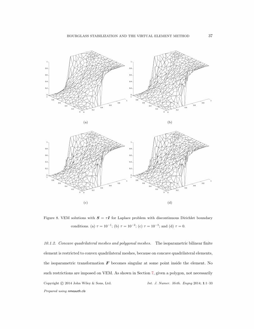
the VEM solution obtained on the second mesh for decreasing τ . We notice the appearance of
hourglass instabilities, even though the scheme does not become singular for τ = 0.
Copyright c© 2014 John Wiley & Sons, Ltd. Int. J. Numer. Meth. Engng 2014; 1:1–33
Prepared using nmeauth.cls

36 CANGIANI ET AL.
10−2
10−1
100
10−5
10−4
10−3
10−2
10−1
Mesh size h
RelativeL2error
1
2
τ = 1
τ = 10
τ = 100
τ = 1000
Figure 6. VEM solution for S = τI, with τ = 1, 10, 100, 1000.
00.2
0.40.6
0.81
0
0.2
0.4
0.6
0.8
10
0.2
0.4
0.6
0.8
1
(a)
00.2
0.40.6
0.81
0
0.2
0.4
0.6
0.8
10
0.2
0.4
0.6
0.8
1
(b)
Figure 7. Laplace problem with discontinuous Dirichlet boundary conditions. (a) Exact solution and
(b) VEM solution for τ = 1.
Copyright c© 2014 John Wiley & Sons, Ltd. Int. J. Numer. Meth. Engng 2014; 1:1–33
Prepared using nmeauth.cls
HOURGLASS STABILIZATION AND THE VIRTUAL ELEMENT METHOD 37
00.2
0.40.6
0.81
0
0.2
0.4
0.6
0.8
10
0.2
0.4
0.6
0.8
1
(a)
00.2
0.40.6
0.81
0
0.2
0.4
0.6
0.8
10
0.2
0.4
0.6
0.8
1
(b)
00.2
0.40.6
0.81
0
0.2
0.4
0.6
0.8
10
0.2
0.4
0.6
0.8
1
(c)
00.2
0.40.6
0.81
0
0.2
0.4
0.6
0.8
10
0.2
0.4
0.6
0.8
1
(d)
Figure 8. VEM solutions with S = τI for Laplace problem with discontinuous Dirichlet boundary
conditions. (a) τ = 10−1; (b) τ = 10−2; (c) τ = 10−3; and (d) τ = 0.
10.1.2. Concave quadrilateral meshes and polygonal meshes. The isoparametric bilinear finite
element is restricted to convex quadrilateral meshes, because on concave quadrilateral elements,
the isoparametric transformation F becomes singular at some point inside the element. No
such restrictions are imposed on VEM. As shown in Section 7, given a polygon, not necessarily
Copyright c© 2014 John Wiley & Sons, Ltd. Int. J. Numer. Meth. Engng 2014; 1:1–33
Prepared using nmeauth.cls

38 CANGIANI ET AL.
(a)
(b)
Figure 9. (a) First and (b) second concave quadrilateral meshes of the sequence.
convex, we can define a finite element space directly on the physical element and compute
using (46)–(49) the VEM stability and consistency matrices.
To demonstrate the behavior of the VEM for concave quadrilaterals, we repeat the test
shown in Figure 5 on the series of meshes obtained from the previous one by subdividing each
quadrilateral into two smaller quadrilaterals, one of which is necessarily concave. The first
two meshes of this new sequence are shown in Figure 9. Convergence curves are presented
in Figure 10 showing that the error norms are almost identical to those obtained on convex
meshes (see Figure 5).
Finally, we report on a numerical experiment for the virtual element decomposition when
applied to the finite element space of generalized barycentric coordinates on polygons as
discussed in Section 7. We consider a sequence of very irregular Voronoi polygonal meshes
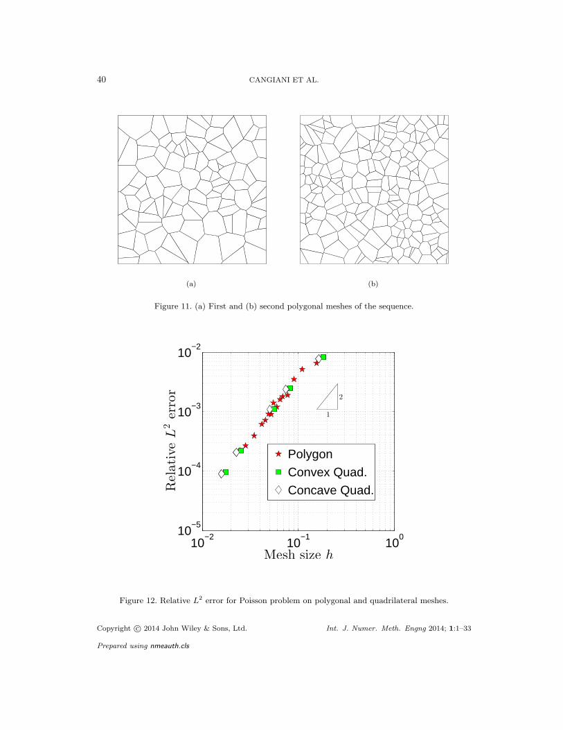
with random seed points; in Figure 11, we show the first and second meshes of the sequence.
Copyright c© 2014 John Wiley & Sons, Ltd. Int. J. Numer. Meth. Engng 2014; 1:1–33
Prepared using nmeauth.cls

HOURGLASS STABILIZATION AND THE VIRTUAL ELEMENT METHOD 39
10−2
10−1
10010
−5
10−4
10−3
10−2
Mesh size h
RelativeL
2error
1
2
Figure 10. Convergence of VEM for the 2D Poisson problem on the concave meshes.
In Figure 12, we present for the purpose of comparison the relative L2 errors on the
quadrilateral (convex and concave) and polygonal meshes, revealing that in the VEM the
error depends as expected on the mesh size, but does not depend on the shape of the elements.
10.2. Three-dimensional problems
In the numerical experiments presented here, we consider three methods:
1. virtual element method (labeled VEM), which corresponds to the stiffness matrix
Kvem = Kvem
c+Kvem
s, where Kvem
cand Kvem
sare defined in (64) and (49), respectively,
with S = heI; for the irregular hexahedral meshes, we use he = |Ωe|1/3.
Copyright c© 2014 John Wiley & Sons, Ltd. Int. J. Numer. Meth. Engng 2014; 1:1–33
Prepared using nmeauth.cls
40 CANGIANI ET AL.
(a)
(b)
Figure 11. (a) First and (b) second polygonal meshes of the sequence.
10−2
10−1
10010
−5
10−4
10−3
10−2
Mesh size h
RelativeL
2error
1
2
Polygon
Convex Quad.
Concave Quad.
Figure 12. Relative L2 error for Poisson problem on polygonal and quadrilateral meshes.
Copyright c© 2014 John Wiley & Sons, Ltd. Int. J. Numer. Meth. Engng 2014; 1:1–33
Prepared using nmeauth.cls

HOURGLASS STABILIZATION AND THE VIRTUAL ELEMENT METHOD 41
2. Flanagan-Belytschko scheme (labeled FB), which corresponds to the stiffness matrix
KFB = KFB
c+KFB
s, where KFB
cand KFB
sare defined in (13) and (25), respectively. We
set ǫ = |Ωe|−2/3 in KFB
sto obtain the correct scaling. Note that Kvem
c= KFB
c.
3. standard isoparametric finite elements with 2×2×2 Gauss quadrature on the reference
biunit cube (labeled ISO-Q1).
Consider the domain Ω = (0, 1)3, which is discretized by a sequence of four unstructured
meshes of decreasing mesh size. Each mesh consists of subdivisions of the unit cube into
highly irregular hexahedra with curved faces. In Table III, the mesh parameters are listed, and
the first two meshes of the sequence are depicted in Figure 13.
Mesh Number of Number of Element
elements nodes diameter h
a 144 243 4.2× 10⁻¹
b 8952 10985 1.2× 10⁻²
c 18580 22365 9.3× 10⁻²
d 82488 95079 5.5× 10⁻²
Table III. Mesh parameters for the unstructured hexahedral meshes.
10.2.1. Patch test First, we show that all three methods pass the patch test. Consider the
nonhomogeneous Dirichlet boundary condition g(x) = 1 − 2x + 3y − 4z in (1) with f = 0
so that u(x) = g(x) is the exact solution. The relative L2 error norms for the three different
methods are listed in Table IV; these results show that all three methods pass the patch test.
Copyright c© 2014 John Wiley & Sons, Ltd. Int. J. Numer. Meth. Engng 2014; 1:1–33
Prepared using nmeauth.cls

42 CANGIANI ET AL.
(a) (b)
Figure 13. Meshes (a) and (b) in the sequence of unstructured hexahedral meshes.
Mesh||u− uh||0,Ω
||u||0,Ω
ISO-Q1 FB [8] VEM
a 2.6× 10⁻¹⁶ 2.7× 10⁻¹⁶ 2.9× 10⁻¹⁶
b 8.1× 10⁻¹⁵ 2.5× 10⁻¹⁵ 2.0× 10⁻¹⁵
c 5.2× 10⁻¹⁶ 4.0× 10⁻¹⁵ 3.2× 10⁻¹⁵
d 5.9× 10⁻¹⁶ 1.0× 10⁻¹⁴ 8.7× 10⁻¹⁵
Table IV. Relative L2 error norms for the patch test in 3D.
10.2.2. Comparison of the methods We consider the Poisson problem with the right-hand-side
f and the Dirichlet boundary value g chosen so that u(x, y, z) = sin(xy) cos(yz)+x3z−ex−3y−z
is the exact solution. In Figure 14, the relative L2 and H1 error curves for the three methods
Copyright c© 2014 John Wiley & Sons, Ltd. Int. J. Numer. Meth. Engng 2014; 1:1–33
Prepared using nmeauth.cls

HOURGLASS STABILIZATION AND THE VIRTUAL ELEMENT METHOD 43
are compared; we observe that all three methods behave very similarly.
10−2
10−1
10010
−4
10−3
10−2
10−1
Mesh size h
RelativeL2error
1
2
VEM
FB [8]
ISO−Q1
(a)
10−2
10−1
10010
−2
10−1
100
Mesh size hRelativeH
1error
1
1
VEM
FB [8]
ISO−Q1
(b)
Figure 14. Rate of convergence of FEM and VEM for the 3D Poisson problem. (a) L2 norm; and (b)
H1 seminorm.
The next numerical experiment is presented to demonstrate that taking S = heI is the
correct scaling for the Poisson problem in three dimensions. To observe the effect of scaling
with respect to the matrix S, fine meshes are needed. Instead, we achieve the same end by
scaling the domain by a factor of 10−2. Then, we consider the VEM with S = I. In Figure 15,
plots of the relative error norms are shown, and we clearly observe that the badly-scaled VEM
does not converge.
Lastly, the effect of scaling S by a very small quantity is studied. As in the two-dimensional
case, we consider a Poisson problem with discontinuous Dirichlet boundary conditions, which
activates the spurious zero-energy modes. In (1), we set f = 0, and g(x, y) = 1 for x < 0.5
and g(x, y) = 0 for x > 0.5 (see Figure 16). We discretize the biunit cube uniformly into
smaller cubes of size he = 1/32, and plot the solutions on the planes z = 2h = 0.0625 and
Copyright c© 2014 John Wiley & Sons, Ltd. Int. J. Numer. Meth. Engng 2014; 1:1–33
Prepared using nmeauth.cls

44 CANGIANI ET AL.
10−4
10−3
10−210
−7
10−6
10−5
10−4
Mesh size h
RelativeL2error
1
2
VEM
VEM (Wrong Scaling)
Figure 15. Relative L2 error for 3D Poisson problem using different choices of the scaling.
z
x
y
z = 2h = 0.0625
z = 16h = 0.5
g = 1g = 0
Figure 16. Laplace problem in 3D with discontinuous Dirichlet boundary conditions.
z = 16h = 0.5. First, we select the correctly-scaled VEM stability matrix; that is, S = heI,
Copyright c© 2014 John Wiley & Sons, Ltd. Int. J. Numer. Meth. Engng 2014; 1:1–33
Prepared using nmeauth.cls

HOURGLASS STABILIZATION AND THE VIRTUAL ELEMENT METHOD 45
00.2
0.40.6
0.81
0
0.2
0.4
0.6
0.8
1
0
0.2
0.4
0.6
0.8
1
(a)
00.2
0.40.6
0.81
0
0.2
0.4
0.6
0.8
1
0
0.2
0.4
0.6
0.8
1
(b)
Figure 17. Virtual element solution for S = h I. (a) z = 0.0625; and (b) z = 0.5.
00.2
0.40.6
0.81
0
0.2
0.4
0.6
0.8
1
0
0.2
0.4
0.6
0.8
1
(a)
00.2
0.40.6
0.81
0
0.2
0.4
0.6
0.8
1
0
0.2
0.4
0.6
0.8
1
(b)
Figure 18. Isoparametric FE solution. (a) z = 0.0625; and (b) z = 0.5.
whose solution is shown in Figure 17. This solution is indistinguishable when compared to the
solution obtained by the ISO-Q1 method (Figure 18). Next, we present results when the VEM
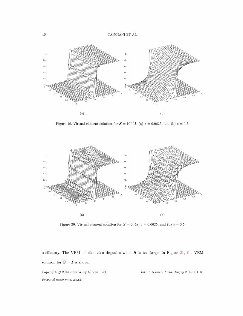
stability term is very small. We choose S = 10−3I in Figure 19 and S = 0 in Figure 20. We
observe that when S = 10−3I oscillations start to develop in the numerical solution, which
degenerates for S = 0. On the contrary, when S = heI = 3.125 × 10⁻²I the solution is not
Copyright c© 2014 John Wiley & Sons, Ltd. Int. J. Numer. Meth. Engng 2014; 1:1–33
Prepared using nmeauth.cls
46 CANGIANI ET AL.
00.2
0.40.6
0.81
0
0.2
0.4
0.6
0.8
1
0
0.2
0.4
0.6
0.8
1
(a)
00.2
0.40.6
0.81
0
0.2
0.4
0.6
0.8
1
0
0.2
0.4
0.6
0.8
1
(b)
Figure 19. Virtual element solution for S = 10−3I. (a) z = 0.0625; and (b) z = 0.5.
00.2
0.40.6
0.81
0
0.2
0.4
0.6
0.8
1
0
0.2
0.4
0.6
0.8
1
(a)
00.2
0.40.6
0.81
0
0.2
0.4
0.6
0.8
1
0
0.2
0.4
0.6
0.8
1
(b)
Figure 20. Virtual element solution for S = 0. (a) z = 0.0625; and (b) z = 0.5.
oscillatory. The VEM solution also degrades when S is too large. In Figure 21, the VEM
solution for S = I is shown.
Copyright c© 2014 John Wiley & Sons, Ltd. Int. J. Numer. Meth. Engng 2014; 1:1–33
Prepared using nmeauth.cls

HOURGLASS STABILIZATION AND THE VIRTUAL ELEMENT METHOD 47
00.2
0.40.6
0.81
0
0.2
0.4
0.6
0.8
1
0
0.2
0.4
0.6
0.8
1
(a)
00.2
0.40.6
0.81
0
0.2
0.4
0.6
0.8
1
0
0.2
0.4
0.6
0.8
1
(b)
Figure 21. Virtual element solution for S = I. (a) z = 0.0625; and (b) z = 0.
11. CONCLUDING REMARKS
In this paper, we showed that the virtual element method (VEM) [16] can be viewed as a
general stabilized underintegrated Galerkin method. We presented a first-order virtual element
approach that was based on isoparametric elements for the Poisson problem in two- and
three-dimensions, and established quantitative connections of this approach with well-known
hourglass stabilization techniques for four-node quadrilateral and eight-node hexahedral finite
elements [8–10].
The robustness and flexibility of the VEM was demonstrated via numerical experiments
on quadrilateral, polygonal (convex and concave elements), and hexahedral meshes. The
importance of the choice and selection of the stability parameter τ was emphasized, and
for suitable choices for τ , optimal convergence rates of the VEM in the L2 norm and the
H1 seminorm of 2 and 1, respectively, were realized. These observations indicate that the
virtual element method provides a systematic and mathematically rigorous approach to develop
Copyright c© 2014 John Wiley & Sons, Ltd. Int. J. Numer. Meth. Engng 2014; 1:1–33
Prepared using nmeauth.cls

48 CANGIANI ET AL.
stable underintegrated finite element methods. Two open-issues that persist with hourglass
control finite element methods are lack of a convergence theory, and suitable choices for
the stabilization parameter τ [10]. The VEM gives definitive answers to these questions:
convergence theory is now available [16] and the theory provides clear guidelines on selecting
τ [23]. Furthermore, the theory is applicable to C0 arbitrary-order polygonal and polyhedral
elements [16], and also to elements that possess arbitrary regularity [26, 27]. Hence, in
such general settings, the virtual element method affords the development of stable and
computationally efficient Galerkin schemes.
In this paper, hourglass stabilization for the Poisson equation was the focus. Recent studies
on the VEM have examined elasticity [28, 29] and plate bending [26]. For vectorial problems,
the number of spurious singular (hourglass) modes substantially increases, which likely makes it
more difficult to draw direct links between VEM and prior work on hourglass control techniques
using the FEM. Further investigations of the VEM for broader classes of partial differential
equations, and in particular for linear and nonlinear solid continua are fruitful directions for
future research.
APPENDIX A
Isoparametric finite elements and the patch test
It is well-known that the bilinear and trilinear isoparametric elements pass the patch test.
In this section, we examine the implications of using a quadrature formula and its effect on
passing or failing the patch test. A similar analysis for the four-node quadrilateral is performed
by Talischi and Paulino [20].
Copyright c© 2014 John Wiley & Sons, Ltd. Int. J. Numer. Meth. Engng 2014; 1:1–33
Prepared using nmeauth.cls
HOURGLASS STABILIZATION AND THE VIRTUAL ELEMENT METHOD 49
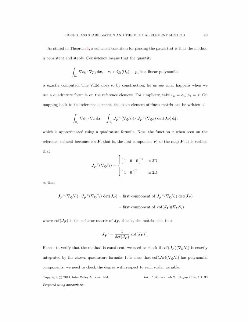
As stated in Theorem 1, a sufficient condition for passing the patch test is that the method
is consistent and stable. Consistency means that the quantity
∫
Ωe
∇vh · ∇p1 dx, vh ∈ Q1(Ωe), p1 is a linear polynomial
is exactly computed. The VEM does so by construction; let us see what happens when we
use a quadrature formula on the reference element. For simplicity, take vh = φi, p1 = x. On
mapping back to the reference element, the exact element stiffness matrix can be written as
∫
Ωe
∇φi · ∇x dx =
∫
Ω0
J−TF (∇ξNi) · J
−TF (∇ξx) det(JF ) dξ,
which is approximated using a quadrature formula. Now, the function x when seen on the
reference element becomes x F , that is, the first component F1 of the map F . It is verified
that
J−T
F (∇ξF1) =
[1 0 0
]Tin 3D,
[1 0
]Tin 2D,
so that
J−T
F (∇ξNi) · J−T
F (∇ξF1) det(JF ) = first component of J−T
F (∇ξNi) det(JF )
= first component of cof(JF )(∇ξNi)
where cof(JF ) is the cofactor matrix of JF , that is, the matrix such that
J−1F =
1
det(JF )cof(JF )
T.
Hence, to verify that the method is consistent, we need to check if cof(JF )(∇ξNi) is exactly
integrated by the chosen quadrature formula. It is clear that cof(JF )(∇ξNi) has polynomial
components; we need to check the degree with respect to each scalar variable.
Copyright c© 2014 John Wiley & Sons, Ltd. Int. J. Numer. Meth. Engng 2014; 1:1–33
Prepared using nmeauth.cls

50 CANGIANI ET AL.
• For the four-node quadrilateral element it can be easily seen that cof(JF )(∇ξNi)
is linear in each component. Hence, any quadrature formula that exactly integrates
functions that are affine in each variable yields a method that is consistent. In fact,
we know that the one-point Gauss rule is consistent but unstable, whereas the 2 × 2
trapezoidal rule is consistent and stable, and therefore passes the patch test.
• For the eight-node hexahedral element it can be observed that cof(JF )(∇ξNi) is
quadratic in each component. Hence, any quadrature formula that exactly integrates
functions that are quadratic in each variable yields a method that is consistent. For
instance, the one-point Gauss rule is inconsistent and unstable, the 2 × 2 × 2 tensor-
product Gauss rule is consistent and stable and therefore passes the patch test, and
the 2 × 2 × 2 trapezoidal rule is inconsistent but stable. For the last case, it can be
numerically shown that the patch test is not passed.
APPENDIX B
B.1. Stencils for the uniform square mesh
On using the energy τ of the function Ψ as a parameter, it is possible to compare the VEM
stiffness matrix in (61) to well-known finite-difference stencils on simple nodal configurations,
and also to fully integrated quadrilateral finite elements. Such comparisons for FEM have been
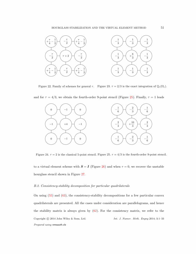
performed in References [9, 10]. For a uniform square mesh, the stencil shown in Figure 22 is
obtained. For a square of side a, we have τ =∫Ωe
|∇Ψ|2 dx = 2/3. With this value of τ , we
obtain the scheme corresponding to the exact integration of the four-node isoparametric finite
element (see Figure 23). On taking τ = 2, we recover the classical 5-point stencil (Figure 24)
Copyright c© 2014 John Wiley & Sons, Ltd. Int. J. Numer. Meth. Engng 2014; 1:1–33
Prepared using nmeauth.cls
HOURGLASS STABILIZATION AND THE VIRTUAL ELEMENT METHOD 51
+τ
4−
1
2−τ
2+τ
4−
1
2
−τ
2τ + 2 −
τ
2
+τ
4−
1
2−τ
2+τ
4−
1
2
Figure 22. Family of schemes for general τ .
−1
3−1
3−1
3
−1
3+8
3−1
3
−1
3−1
3−1
3
Figure 23. τ = 2/3 is the exact integration of Q1(Ωe).
and for τ = 4/3, we obtain the fourth-order 9-point stencil (Figure 25). Finally, τ = 1 leads
0 −1 0
−1 +4 −1
0 −1 0
Figure 24. τ = 2 is the classical 5-point stencil.
−1
6−2
3−1
6
−2
3+10
3−2
3
−1
6−2
3−1
6
Figure 25. τ = 4/3 is the fourth-order 9-point stencil.
to a virtual element scheme with S = I (Figure 26) and when τ = 0, we recover the unstable
hourglass stencil shown in Figure 27.
B.2. Consistency-stability decomposition for particular quadrilaterals
On using (55) and (63), the consistency-stability decompositions for a few particular convex
quadrilaterals are presented. All the cases under consideration are parallelograms, and hence
the stability matrix is always given by (62). For the consistency matrix, we refer to the
Copyright c© 2014 John Wiley & Sons, Ltd. Int. J. Numer. Meth. Engng 2014; 1:1–33
Prepared using nmeauth.cls

52 CANGIANI ET AL.
−1
4−1
2−1
4
−1
2+3 −
1
2
−1
4−1
2−1
4
Figure 26. τ = 1 is a virtual element scheme.
−1
20 −
1
2
0 +2 0
−1
20 −
1
2
Figure 27. τ = 0 gives the unstable hourglass stencil.
decomposition (55).
• Square with side a:
U =1
4a2
2a2 0
0 2a2
=
1/2 0
0 1/2
,
∫
Ωe
|∇Ψ|2 dx = 2/3
• Rectangle with base a and height b:
U =1
4ab
a2 + b2 a2 − b2
a2 − b2 a2 + b2
,
∫
Ωe
|∇Ψ|2 dx =a2 + b2
3ab.
• Rhombus with side a and angle θ at vertex 1:
U =1
4a2 sin θ
2a2(1− cos θ) 0
0 2a2(1 + cos θ)
=
1− cos θ
2 sin θ0
01 + cos θ
2 sin θ
,
∫
Ωe
|∇Ψ|2 dx =2
3 sin θ.
• Parallelogram with base a, oblique side b, and angle θ at vertex 1:
U =1
4ab sin θ
a2 − 2ab cos θ + b2 a2 − b2
a2 − b2 a2 + 2ab cos θ + b2
,
∫
Ωe
|∇Ψ|2 dx =a2 + b2
3ab sin θ.
Copyright c© 2014 John Wiley & Sons, Ltd. Int. J. Numer. Meth. Engng 2014; 1:1–33
Prepared using nmeauth.cls
HOURGLASS STABILIZATION AND THE VIRTUAL ELEMENT METHOD 53
ACKNOWLEDGEMENTS
The authors thank Franco Brezzi and Donatella Marini for their many valuable comments and
suggestions. A. C. gratefully acknowledges support from the College of Science and Engineering
of the University of Leicester and the support of the EPSRC (Grant EP/L022745/1). G. M.
gratefully acknowledges support of the LDRD-ER Project #20140270 “From the finite element
method to the virtual element method” at the Los Alamos National Laboratory and of the
DOE Office of Science Advanced Scientific Computing Research (ASCR) Program in Applied
Mathematics Research. A. R. gratefully acknowledges the research support from the University
of Milano-Bicocca. N. S. gratefully acknowledges the research support of the National Science
Foundation through contract grant CMMI-1334783 to the University of California at Davis.
REFERENCES
[1] L. M. Taylor and D. P. Flanagan. PRONTO 2D: A two-dimensional transient solid
dynamics program. Technical report, Sandia National Laboratories, Albuquerque, NM,
USA, 1987.
[2] L. M. Taylor and D. P. Flanagan. PRONTO 3D: A three-dimensional transient solid
dynamics program. Technical report, Sandia National Laboratories, Albuquerque, NM,
USA, 1989.
[3] J. O. Hallquist. LS-DYNA3D theoretical manual. Technical report, Livermore Software
Technology Corporation, Livermore, CA, USA, 1993.
[4] R. L. Taylor. FEAP – A Finite Element Analysis Program Ver-
Copyright c© 2014 John Wiley & Sons, Ltd. Int. J. Numer. Meth. Engng 2014; 1:1–33
Prepared using nmeauth.cls

54 CANGIANI ET AL.
sion 8.4 User Manual, 2013. University of California, Berkeley.
(http://www.ce.berkeley.edu/projects/feap/manual84.pdf) [Accessed on January
10, 2014].
[5] Hibbitt, Karlsson & Sorensen, Inc. ABAQUS/Standard, 2004. User’s Manual, Version 6.5,
Pawtucket, Rhode Island, USA.
[6] S. W. Key. A finite element procedure for the large deformation dynamics response of
axisymmetric solids. Computer Methods in Applied Mechanics and Engineering, 4:195–
218, 1978.
[7] D. Kosloff and G. A. Frazier. Treatment of hourglass patterns in low order finite element
codes. International Journal for Numerical and Analytical Methods in Geomechanics,
2:57–72, 1978.
[8] D. P. Flanagan and T. Belytschko. A uniform strain hexahedron and quadrilateral
with orthogonal hourglass control. International Journal for Numerical Methods in
Engineering, 17(5):679–706, 1981.
[9] W. K. Liu and T. Belytschko. Efficient linear and nonlinear heat conduction with a
quadrilateral element. International Journal for Numerical Methods in Engineering,
20(5):931–948, 1984.
[10] T. Belytschko, J. S.-J. Ong, W. K. Liu, and J. M. Kennedy. Hourglass control in linear
and nonlinear problems. Computer Methods in Applied Mechanics and Engineering,
43(3):251–276, 1984.
Copyright c© 2014 John Wiley & Sons, Ltd. Int. J. Numer. Meth. Engng 2014; 1:1–33
Prepared using nmeauth.cls

HOURGLASS STABILIZATION AND THE VIRTUAL ELEMENT METHOD 55
[11] T. Belytschko and W. E. Bachrach. Efficient implementation of quadrilaterals with
high coarse-mesh accuracy. Computer Methods in Applied Mechanics and Engineering,
54(3):279–301, 1986.
[12] O.-P. Jacquotte and J. T. Oden. Analysis of hourglass instabilities and control in
underintegrated finite element methods. Computer Methods in Applied Mechanics and
Engineering, 44:339–363, 1984.
[13] W. K. Liu, J. S.-J. Ong, and R. A. Uras. Finite element stabilization matrices —
a unification approach. Computer Methods in Applied Mechanics and Engineering,
53(1):13–46, 1985.
[14] B. C. Koh and N. Kikuchi. New improved hourglass control for bilinear and trilinear
elements in anisotropic linear elasticity. Computer Methods in Applied Mechanics and
Engineering, 65:1–46, 1987.
[15] T. B. Belytschko, W. K. Liu, and B. Moran. Nonlinear Finite Elements for Continua
and Structures. John Wiley and Sons, New York, 2000.
[16] L. Beirao da Veiga, F. Brezzi, A. Cangiani, G. Manzini, L. D. Marini, and A. Russo.
Basic principles of virtual element methods. Mathematical Models & Methods in Applied
Sciences, 23(1):199–214, 2014.
[17] G. L. Goudreau and J. O. Hallquist. Recent developments in large-scale finite-
element Lagrangian hydrocode technology. Computer Methods in Applied Mechanics and
Engineering, 33(1–3):725–757, 1982.
Copyright c© 2014 John Wiley & Sons, Ltd. Int. J. Numer. Meth. Engng 2014; 1:1–33
Prepared using nmeauth.cls

56 CANGIANI ET AL.
[18] L. Beirao da Veiga, F. Brezzi, L.D. Marini, and A. Russo. The hitchhiker’s guide to the
virtual element method. Mathematical Models & Methods in Applied Sciences, 24(8):1541–
1573, 2014.
[19] G. Manzini, A. Russo, and N. Sukumar. New perspectives on polygonal and polyhedral
finite element methods. Mathematical Models & Methods in Applied Sciences, 24(8):1665–
1699, 2014.
[20] C. Talischi and G. H. Paulino. Addressing integration error for polygonal finite element
through polynomial projections: A patch test connection. Mathematical Models & Methods
in Applied Sciences, 24(8):1701–1727, 2014.
[21] K. Lipnikov, G. Manzini, and M. Shashkov. Mimetic finite difference method. Journal of
Computational Physics, 257 – Part B:1163–1227, 2014.
[22] L. Beirao da Veiga, K. Lipnikov, and G. Manzini. The Mimetic Finite Difference Method,
volume 11 of Modeling, Simulations and Applications. Springer-Verlag, New York, I
edition, 2013.
[23] B. Ahmad, A. Alsaedi, F. Brezzi, L.D. Marini, and A. Russo. Equivalent projectors for
virtual element methods. Computer & Mathematics with Applications, 66(3):376–391,
2013.
[24] P. Hansbo. A new approach to quadrature for finite elements incorporating hourglass
control as a special case. Computer Methods in Applied Mechanics and Engineering,
158(3):301–309, 1998.
Copyright c© 2014 John Wiley & Sons, Ltd. Int. J. Numer. Meth. Engng 2014; 1:1–33
Prepared using nmeauth.cls

HOURGLASS STABILIZATION AND THE VIRTUAL ELEMENT METHOD 57
[25] T. Belytschko. Correction of article by D.P. Flanagan and T.Belytschko. International
Journal for Numerical Methods in Engineering, 19(3):467–468, 1983.
[26] F. Brezzi and L. D. Marini. Virtual element methods for plate bending problems.
Computer Methods in Applied Mechanics and Engineering, 253:455–462, 2013.
[27] L. Beirao da Veiga and G. Manzini. A virtual element method with arbitrary regularity.
IMA Journal on Numerical Analysis, 34(2):759–781, 2014.
[28] L. Beirao da Veiga, F. Brezzi, and L. D. Marini. Virtual elements for linear elasticity
problems. SIAM Journal on Numerical Analysis, 51(2):794–812, 2013.
[29] A. Gain, C. Talischi, and G. H. Paulino. On the virtual element method for three-
dimensional linear elasticity problems on arbitrary polyhedral meshes. Computer Methods
in Applied Mechanics and Engineering, 282:132–160, 2014.
Copyright c© 2014 John Wiley & Sons, Ltd. Int. J. Numer. Meth. Engng 2014; 1:1–33
Prepared using nmeauth.cls