HOT-WIRE MEASUREMENTS OF INSTABILITY WAVES ON A BLUNT CONE AT MACH-6

AIAA Paper 2005-5137, Presented at the 35th Fluid Dynamics Conference, Toronto, Canada, June 2005.

Shann J. Rufer* and Steven P. Schneider† School of Aeronautics and Astronautics

Purdue University West Lafayette, IN 47906

Hot wire calibrations were completed in the supersonic jet facility at Purdue University. This jet consists of a Mach-4 nozzle and allows for a continuous run time. The hot wires were calibrated under conditions similar to those seen in the Mach-6 facility at Purdue University. These hot wires were then used in the Mach-6 tunnel to study the amplitude and growth of instability waves on 7-deg half-angle sharp and blunt cones.

INTRODUCTION

The process of transition is not completely understood, even after years of research. The study of transition in the hypersonic flow regime becomes important due to the effect of transition on separation, heat transfer, and other boundary layer parameters. Though transition location can often be determined, the disturbance mechanisms which cause transition and the relationship between instability and transition remain uncertain [1]. As discussed in Ref. [2], very few accurate experimental studies of instability-wave growth have been conducted in hypersonic flow and an even smaller number of these have been completed with calibrated instrumentation. In hypersonic flow, there are four basic instability mechanisms which produce disturbance growth: (1) first mode, or Tollmien-Schlichting, (2) second mode, or Mack mode, (3) cross-flow, and (4) Görtler [1]. The second mode instabilities, the most unstable of the Mack modes, tend to become dominant in hypersonic flow on symmetric models without concave curvature [3]. The second mode instability tends to occur at high frequencies when the boundary layer is ‘thin’ and at low frequencies for ‘thick’ boundary layers [4] and is most amplified when it is axisymmetric [5]. *Research Assistant. Student Member, AIAA. †Professor. Associate Fellow, AIAA. Copyright ©2005 by Steven P. Schneider. Published by the American Institute of Aeronautics and Astronautics, Inc., with permission.

Transition on Blunt Cones In hypersonic flow it is important to have a blunt leading edge in order to control the heating of the nose region of the vehicle. The effects of bluntness can be experienced by the flow hundreds of nosetip radii downstream. The actual distance that the effects seem to propagate is dependent on the bluntness and freestream conditions [6]. Leading edge bluntness also influences viscous-inviscid interaction, flow separation, pressure and velocity distributions, skin friction, heat transfer, etc. Boundary-layer transition occurs in a fluid flow as instabilities in the flow cause small disturbances to grow, which in turn causes the flow to shift (transition) from laminar to turbulent. Transition involves many uncertainties and is therefore a very complex problem to solve. To alleviate some of the complexity, many experiments have been conducted on hypersonic boundary layer transition. These experiments assess numerous parametric trends, such as the effects of Mach number, nosetip bluntness, and unit Reynolds number, as well as many others. A layer of high specific entropy and strong entropy gradients in the gas outside the boundary layer, commonly referred to as an entropy layer, is introduced into the flow downstream of the blunt nose (see Figure 1). This layer is a region of high temperature, low-density gas created by the large entropy increase in the gas as it passes through the bow shock caused by the bluntness on the leading edge [7]. The thickness of this layer is a direct function of the bluntness on the

1

leading edge of the vehicle [6]. The entropy layer is important because of its effect on the growth of the viscous layer. When bluntness causes an entropy layer to be introduced into the flow, the growth of the viscous layer changes, and it grows through interaction with the entropy layer [8]. These new entropy effects also promote changes of the flow properties in the boundary layer and introduce a velocity and pressure gradient at the outer edge of the boundary layer [6]. The variable entropy effects caused by nose bluntness are ‘swallowed’ by the boundary layer at a certain length (termed the swallowing length) downstream of the nose. This, in turn, changes the properties of the boundary layer and the point at which transition occurs [8].

Figure 1 – A schematic diagram of supersonic flow over a blunt cone [10]. The effects of nose bluntness can be broken into two separate cases, that of ‘small bluntness’ and ‘large bluntness’ [9], [10]. In the small bluntness case, transition occurs behind the point where the entropy layer is swallowed by the boundary layer. For this case, the transition Reynolds number increases with increasing bluntness and the point of transition moves aft on the body. For the large bluntness case, where transition occurs forward of the swallowing distance, the transition Reynolds number decreases rapidly with increasing bluntness and transition moves forward on the body. It was determined in Ref. [11] that in the case of small nosetip bluntness, increases in bluntness helped in the stabilization of the boundary layer.

It was shown in Ref. [4], through several transition experiments with nosetip radii of 0.15, 0.25, 0.5, and 0.7 inches, that a small bluntness on the vehicle nosetip can considerably increase the transition Reynolds number due to large increases in the critical Reynolds number (the Reynolds number beyond which the disturbances become unstable). For small nose radii (both 0.15 and 0.25 inches), the boundary layer appeared to be stable within the entropy-layer-swallowing region and the location of the critical Reynolds number seemed to coincide with the entropy-swallowing location, though the critical Reynolds number was not determined for the 0.25 inch radii nosetip. Ref. [12] states that the reason there is a stabilizing influence on the boundary layer is because “the effect of leading edge bluntness is to decrease the local Mach number, which would bring the boundary layer closer to separation, while at the same time lowering the local Reynolds number and increasing the favorable pressure gradient”. Ref. [4], however, also demonstrated that a growth in the boundary layer disturbances at small local Reynolds number and a destabilization of the boundary layer occurred when further increases in the bluntness of the nosetip were made. The reasons for this phenomenon seem unclear. Boeing/Air Force Mach-6 Quiet-Flow Ludwieg Tube The present study of boundary layer transition and instability waves on cones was conducted in the Purdue Mach-6 Quiet-Flow Ludwieg Tube. A Ludwieg Tube is similar to the more common shock tunnel. It consists mainly of a long pipe, or driver tube, a converging-diverging nozzle, and a set of burst diaphragms. The flow exits the nozzle into the test section and diffuser, which is connected to a large vacuum tank. The vacuum tank is separated from the pressurized upstream section of the tunnel by a set of diaphragms. When the differential pressure across the diaphragms becomes great enough, the diaphragms will burst. This causes a shock wave to travel downstream, into the vacuum tank, and an expansion wave to travel upstream, into the test section and driver tube, initiating hypersonic flow.

2

The Purdue Mach-6 Quiet-Flow Ludwieg Tube (see Figure 2 through Figure 4) operates on this principle. The driver tube is 17.5 inches in diameter and 122.5 feet long, and is connected to a tapered contraction section. A bleed slot is located near the end of the contraction section to bleed off the boundary layer before the flow enters the nozzle throat. The diaphragms are placed in the tunnel downstream of the test section and used to initiate the flow. Once the diaphragms have burst, there is, on average, a seven-second run before the pressure ratio is insufficient and the flow drops subsonic.

Figure 2 – Nozzle section of the Purdue Mach-6 Quiet Flow Ludwieg Tube.

Figure 3 – Test and diffuser sections of the Purdue Mach-6 Quiet Flow Ludwieg Tube.

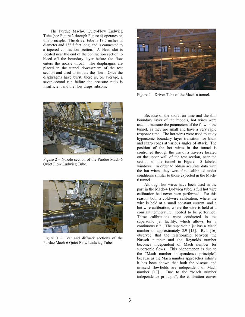
Figure 4 – Driver Tube of the Mach-6 tunnel.

Because of the short run time and the thin boundary layer of the models, hot wires were used to measure the parameters of the flow in the tunnel, as they are small and have a very rapid response time. The hot wires were used to study hypersonic boundary layer transition for blunt and sharp cones at various angles of attack. The position of the hot wires in the tunnel is controlled through the use of a traverse located on the upper wall of the test section, near the section of the tunnel in Figure 5 labeled windows. In order to obtain accurate data with the hot wires, they were first calibrated under conditions similar to those expected in the Mach-6 tunnel. Although hot wires have been used in the past in the Mach-4 Ludwieg tube, a full hot wire calibration had never been performed. For this reason, both a cold-wire calibration, where the wire is held at a small constant current, and a hot-wire calibration, where the wire is held at a constant temperature, needed to be performed. These calibrations were conducted in the supersonic jet facility, which allows for a continuous run. The supersonic jet has a Mach number of approximately 3.9 [15]. Ref. [16] observed that the relationship between the Nusselt number and the Reynolds number becomes independent of Mach number for supersonic flows. This phenomenon is due to the “Mach number independence principle”, because as the Mach number approaches infinity it has been shown that both the viscous and inviscid flowfields are independent of Mach number [17]. Due to the “Mach number independence principle”, the calibration curves

3

obtained using the Mach-4 jet can be applied to the data obtained from the hot wires in the Mach-6 tunnel. Due to the high stagnation temperature of the Mach-6 tunnel, needed to ensure that liquefaction does not occur, the hot wire needs to be able to withstand very high temperatures. The overheat ratio, the temperature of the wire divided by the stagnation temperature, needs to be set to a value near 1.0 (2.0 if measured by resistances) so that the hot wire becomes more

sensitive to mass-flow-rate fluctuations. This overheat ratio causes the wire temperature to be approximately 400-550K. For this reason, the material being used for the hot wire had to be chosen carefully. Tungsten, which had previously been used in the Mach-4 Ludweig tube, has an oxidation temperature of about 600K, above which the wire burns out. Platinum-10% Rhodium wires were tested and have to date survived temperatures of close to 870K.

Figure 5 - Schematic of the Mach 6 Purdue Quiet Flow Ludwieg Tube

HOT-WIRE INSTRUMENTATION The hot wires are calibrated in the supersonic jet at the Purdue Aerospace Science Laboratory. A Mach 4 nozzle was designed and built for this purpose [18]. The Mach-4 nozzle allows for a continuous run with a 2.5-cm diameter test nozzle at approximately Mach 3.9. The stagnation pressure and temperature in the jet can be varied independently and each is

measured using precision gauges. The pressure in the plenum section is measured using an Ashcroft temperature compensated test gauge with a range of 0-100 psia and an accuracy of 0.25%. The temperature in the plenum is measured with a Fluke thermometer and a J-type thermocouple. To obtain accurate calibrations in the jet, the flow must be characterized using Kulite pressure probes and hot-wire instrumentation. The hot

4

wire and Kulite probes can be placed in the center of the nozzle exit flow by using the traverse seen in Figure 6. The Mach and pressure profiles of the jet were obtained using a Kulite Pitot probe. The Kulite was placed in the center of the nozzle exit flow and connected to custom-built electronics. The pressure of the tunnel was then varied

between 16.5 and 44.5 psia in 2 psi increments. A second set of data for this pressure range was then obtained to determine the repeatability of the measurements. The Mach number, mean Pitot pressure, and percent rms noise were then calculated and the results are reported in Ref. [19].

Figure 6 - Supersonic jet with hot wire positioned at the centerline of the exit plane

When connected to the low-current constant current anemometer, the wire acts as a cold wire and the temperature profile of the flow can be obtained. The probe is then attached to the constant temperature anemometer which heats the wire to an elevated temperature and hot wire measurements can be obtained. This data can then be used to determine the mass flow profile of the tunnel which can then be used to calculate the Nusselt vs. Reynolds number calibration curve. The preliminary calibration of the hot wires is discussed in detail in Refs [20] and [21]. The data obtained from these calibrations were plotted against data digitized from the plots of Weltmann and Kuhns [22] and though the Nusselt vs. Reynolds number data seemed to follow a similar pattern the Nusselt number for a given Reynolds number was approximately 75% larger [21]. Currently, a Mach 4 nozzle is being used in the supersonic jet. According to Otaola [23] and Schneider [18], the fluctuations with this nozzle were too large, in part due to a small gap

between the contraction and nozzle sections. A second nozzle, for Mach 6 flow, has been machined and was tested by Otaola, but the heater plumbing used with this nozzle does not allow for the desired temperatures to be reached in the jet (temperatures comparable to that of the Mach 6 tunnel). It is possible that band heaters placed on the plenum section could solve this problem. In order to make more accurate calibrations in the supersonic jet, the Mach-4 nozzle has been partially redesigned to allow for smaller fluctuations and improved flow conditions. This new design removed the gap which existed between the contraction and nozzle sections, provides more reliably smooth flow surfaces, and has allowed for better sealing conditions. This new design has helped to eliminate the high fluctuations levels seen in the jet; the fluctuations are now at a normal level of about 2% or less. A new set of calibration data was then needed to determine if the reduction of the fluctuation levels in the jet could reduce the differences seen between measurements obtained

5

in the jet and those obtained by Weltmann and Kuhns [22] and Baldwin [16]. The hot wire, hot wire Y, used for the calibration procedure is made of Platinum/10% Rhodium (Pt/Rh), with a diameter of 0.00015 in., a length/diameter ratio of approximately 157 and a cold resistance of 11.63 ohms. The hot wire was placed in the center of the nozzle exit flow and the leads were connected to the constant current anemometer. The chamber pressure was varied from 10 to 30 psig in 2 psi increments and the stagnation temperature was approximately 430K. The mean voltage was measured with an HP digital multimeter, model number 34401A. Once the temperature profile was obtained, the hot wire was connected to the 1:1 bridge of the TSI IFA-100 constant temperature anemometer in order to acquire a mass flux profile. The overheat ratio, based on resistances, was set to 1.75 and the square-wave frequency response, as measured in still air at ambient pressure, was 205 kHz. The chamber pressure was again varied from 10 to 30 psig and the stagnation temperature held near 430K. All data was collected using a LeCroy oscilloscope with a sampling frequency of 1 MHz. Once the Nusselt and Reynolds numbers were determined, they were once again plotted against the data found previously by Weltmann and Kuhns [22], as shown in Figure 7. As seen in this figure, the current data falls in line with previous data and helps to validate the present calibration procedure. The Knudson number and temperature recovery ratio were also determined from the current calibration data and are plotted in Figure 8, along with similar data from Weltmann and Kuhns [22]. The current temperature recovery ratio for a given Knudson number is slightly lower than that found previously; however, it does not seem to be a significant difference. A second hot wire, hot wire X with a cold resistance of 12.56 Ω and an aspect ratio of approximately 154, was then placed in the supersonic jet to be calibrated, however a full calibration was not completed as problems with the heater arose before a mass flux profile was obtained. The data acquired from the cold wire calibration allowed for determination of the Knudson number and temperature recovery ratio and these are also included in the plot in Figure 8. As seen here, the curves for the two wires are very similar in nature.

10-2

10-1

100

101

102

10310

-2

10-1

100

101

102

Wire Reynolds Number

Nus

selt

Num

ber

.0011

.0031

.0050

.0156

.0620

.148

.492ref8ref13AR=157

Figure 7 – Nusselt/Reynolds number calibration curve comparison. Present data is ‘AR=157’, other data presented in Welmann and Kuhns [22].

10-2

10-1

100

101

1020.95

1

1.05

1.1

1.15

1.2

1.25

Knudson Number

Tem

pera

ture

Rec

over

y.0011.0031.0050.0156.0620ref8ref13AR=154AR=157

Figure 8 – Knudson number versus temperature recovery ratio. Present data is ‘AR=154’ and ‘AR=157’, other data presented in Weltmann and Kuhns [22]. HOT WIRE MEASUREMENTS ON SHARP

CONES

Hot wire measurements were conducted to study the effect of axial location upon the instability waves on a 7° half-angle sharp cone at zero angle of attack. The cone is approximately 16.3 inches in length and has a base diameter of 4 inches. The first set of measurements was obtained using hot wire A (hwA) which has a cold resistance of approximately 9.9 Ω. This wire is Pt-10%Rh with a diameter of 0.00015

6

inches and a length to diameter ratio of approximately 135. The hot wire was placed 10.3 and 12.3 inches axially downstream from the tip of the cone. This axial location of the hot wire is defined as z. An illustration of the hot wire near the cone wall is shown in Figure 9. A TSI-IFA 100 constant temperature anemometer was used and the overheat ratio was set to near

1.9, based on resistances. The square wave frequency response was 255 kHz, as measured in still air at ambient pressure. The driver temperature was set to 433K for these runs and the dew point measured for these runs (and all other runs) was normally in the range of -22 to -27°C.

Figure 9 – Hot wire located near the cone wall in the test section of the Purdue Mach-6 Ludwieg Tube.

To avoid electrical noise from the traverse motor, each run consisted of one height above the cone wall with the hot wire initially placed at 1.0 mm above the cone wall. These distances were measured using an Infinity Model K2 long-distance microscope with a CF-1B objective lens. An additional set of lenses is used to correct for distortion caused by the curvature of the thick Plexiglas window. After each run the traverse motor was engaged and the hot wire moved further away from the cone wall. The data was sampled at 1 MHz for 2 seconds (13 bit resolution) using a Tektronix TDS7104 digital oscilloscope in Hi-Res mode (TDS7000 Manual). In Hi-Res mode, data is sampled at 1 GHz and averaged on the fly into memory at the sampling rate. This mode provides additional resolution and digital filtering, both important for some of the data presented. All data were analyzed for the same time-step (0.40-0.45 seconds) during the run.

Figure 10 shows the frequency spectra for hwA with an initial driver pressure of 125 psia and an axial location of z=12.3 inches. From this figure an apparent second mode instability wave can be seen at a frequency of approximately 250kHz. Figure 11 shows a comparison between the spectra for two axial locations, 10.3 and 12.3 inches aft of the nosetip. It is clear in this Figure that the maximum amplitude of the wave occurs when the hot wire is located at the most aft position. The frequency of the apparent second mode wave occurs at a higher frequency (~275kHz) when the hot wire is positioned in the thinner boundary layer at 10.3 inches aft of the nosetip. This decrease in frequency with downstream distance is as expected.

7

0 1 2 3 4 5

x 105

10−6

10−5

10−4

10−3

10−2

10−1

100

frequency (Hz)

y = 1.0 mmy = 1.2 mmy = 1.4 mmy = 1.6 mm

Figure 10 – Frequency Spectra on 7° sharp cone at 125 psia with the hot wire located at z=12.3 inches, hwA, y is the height above the cone wall.

0 1 2 3 4 5

x 105

10−6

10−5

10−4

10−3

10−2

10−1

100

frequency (Hz)

z=10.3"z=12.3"

Figure 11 – Comparison of spectra near boundary layer edge at different axial locations along the length of the cone at 125 psia, taken with hwA.

A second longer sharp cone, with a total length of 22.4 inches and a base diameter of 5.5 inches, was used with hot wire X (hwX), which has a cold resistance of approximately 12.56 Ω and a length to diameter ratio of approximately 154. The hot wire was placed 11.75, 14.0, and 16.7 inches axially downstream from the tip of the cone. A TSI-IFA 100 constant temperature anemometer was used and the overheat ratio was

set to near 1.78. The square wave frequency response was 210 kHz, as measured in still air at ambient pressure. For each axial location of the hot wire, a series of runs were conducted at several different heights above the cone wall.

Figures 12 and 13 are examples of the boundary layer profile and frequency spectra obtained at each axial location. These figures were obtained from the runs conducted with the

8

hot wire located 11.75 inches aft of the nosetip. As illustrated in Figure 12, the mean voltage increases as the hot wire is moved away from the wall until a maximum value is reached, which indicates the edge of the boundary layer. The value of the mean voltage outside of the boundary layer is relatively constant, though there is a slightly decreasing trend until the end of the run.

Variations in the amplitudes of the hot wire fluctuations are shown as a function of the height above the cone in the power spectra of Figure 13. There appears to be an instability wave occurring near 240 kHz. This instability wave is not present near the wall, but as the distance from the wall is increased the amplitude also increases until reaching its peak at approximately 1.75 mm, near the edge of the boundary layer, as expected. Then as the height is further increased the amplitude of the wave decreases and is no longer present in the spectra obtained with the hot wire in the freestream flow. The sharp spike seen at 300 kHz is present for all locations except 1.0 mm and is thought to be due to a flaw in the hot wire.

The hot wire was moved aft to approximately 14, and then 16.7 inches, and the process was repeated. Figure 14 shows a comparison between the power spectra for the three axial locations. The data plotted is from the height above the wall which is nearest the

edge of the boundary layer. As seen in this figure, the amplitude of the wave increases and the frequency decreases, as expected, as the hot wire is moved further aft of the nosetip. The spectrum shown for the z=16.7 location indicates that laminar-turbulent transition occurred somewhere between 14 and 16.7 inches aft of the nosetip, as the instability is no longer present at 16.7 inches.

1 2 3 4 5 6 70.9

1

1.1

1.2

1.3

1.4

height above cone (mm)

mea

n vo

ltage

mean

1 2 3 4 5 6 70

0.02

0.04

0.06

0.08

0.1

RM

S vo

ltage

rms

Figure 12 – Boundary layer profile on a sharp cone at 0° AOA, with a driver pressure of 90 psia and the hot wire located 11.75 inches aft of the nosetip.

0 100 200 300 400 500

10-6

10-4

10-2

frequency (kHz)

y=1.0mmy=1.25y=1.5y=1.75y=2.0y=7.0

Figure 13 – Frequency spectra showing apparent second mode waves – data obtained with the hot wire located 11.75 inches aft of the nosetip on a sharp cone and 0° AOA.

9

50 100 150 200 250 300 350 400 450 500

10-6

10-4

10-2

frequency (kHz)

z=11.75 inz=14.0z=16.7

Figure 14 – Comparison of frequency spectra from different axial locations on a sharp cone at 0° AOA and 90 psia

HOT WIRE MEASUREMENTS ON BLUNT CONES

A 22.25 inch long blunt cone, with a 7° half-angle, was also used for testing in the Mach-6 tunnel. This cone has a 5.5 inch base diameter and a nosetip radius of 0.020 inches. The cone was machined in three different pieces and the pieces were assembled using socket-head cap screws. The screws are placed in the center shaft of the cone and threaded into the cone pieces to draw the sections together in a tight fit. The maximum step between the joints was 0.0005 inches. The base section was machined out of aluminum, the midcone section of 15-5 Stainless Steel H1025, and the nosecone section of 15-5 Stainless Steel H1150. The cone was placed in the test section of the tunnel at a zero angle of attack and hot wire X, which has a cold resistance of 12.56 Ω and an aspect ratio of approximately 154, was placed at several different axial locations downstream of the nose. The overheat ratio (based on resistances) was set to 1.78 and the square wave frequency response was 210 kHz, as measured in still air at ambient pressure. Each run consisted of one height above the wall and all measurements were taken for the same time-step

(0.40-0.45) during the run. The initial driver pressure for each run was set to 45 psia and the driver temperature to 433K. The hot wire was originally placed 20 inches aft of the nosetip at a height of 2.0 mm above the cone. Once this first run was completed, the hot wire was moved a quarter of a millimeter further from the cone wall and second run was completed. This process was then repeated until a height of 4.0 mm was reached. The mean and rms voltages obtained from this series of runs are shown in Figure 15. As seen in this figure, the mean voltage rises as the height of the hot wire increases until a height of approximately 3.0 mm is reached, at which point the mean voltage seems to level off. This indicates that the edge of the boundary layer on the cone is located approximately 3.0 mm above the cone wall at this axial location. The peak in rms occurs closer to the wall than expected but this could be resolved, at least in part, by conducting more runs in smaller height increments near the boundary layer edge.

10

2 2.5 3 3.5 40.8

0.9

1

1.1

height above cone (mm)

mea

n vo

ltage

mean

2 2.5 3 3.5 40

0.02

0.04

0.06

RM

S v

olta

ge

rms

Figure 15 - Boundary layer profile on a blunt cone at 0° AOA, with a driver pressure of 45 psia and the hot wire located 20 inches aft of the nosetip. The variation of the instabilities as a function of height above the cone is illustrated in Figures 16 and 17. The instability occurs around 130 kHz and the amplitude increases until reaching its peak at approximately 2.75 mm. No apparent instability is present until the hot wire

reaches a height of 2.25 mm above the wall. Figure 17 is a close-up of these spectra and better shows the variation of the instability with height. Again there are several sharp spikes in the spectra which are present at all heights above the cone, except those nearest the cone wall. As stated previously, these spikes are thought to be caused by a flaw in the hot wire and future runs will be conducted with a different hot wire to observe if they are still present. The growth of the instabilities as a function of axial location is illustrated in Figure 18. This figure shows the spectra found nearest the edge of the boundary layer (location of maximum amplification) for three different axial locations. As seen here, when the hot wire is located 18 inches aft of the nosetip, the instability is lower in amplitude and occurs at a higher frequency then at the 20 inch location. Transition seems to occur between 20 and 22 inches aft of the nosetip, as somewhere between these locations no instability is present and the amplitude of the spectra is greater than at the two previous locations.

0 100 200 300 400 500

10-6

10-4

10-2

frequency (kHz)

y=2.0 mmy=2.25y=2.5y=2.75y=3.0y=3.25y=4.0

Figure 16 – Frequency spectra showing apparent second mode waves – data obtained with the hot wire

located 20 inches aft of the nosetip on a bunt cone and 0° AOA.

11

60 80 100 120 140 160 180 200 220 24010-6

10-5

10-4

10-3

frequency (kHz)

y=2.0 mmy=2.25y=2.5y=2.75y=3.0y=3.25y=4.0

Figure 17 – Close-up of the power spectra for a 7° blunt cone at zero angle of attack

0 100 200 300 400 500

10-6

10-4

10-2

frequency (kHz)

z=18 inz=20z=22

Figure 18 - Comparison of frequency spectra from different axial locations on a blunt cone at 0° AOA and

45 psia

CONCLUSIONS Hot wire calibrations have been completed using the supersonic jet and the resulting calibration curves seem to be similar to those presented in Weltmann and Kuhns [22]. These calibrations curves will allow for

characterization of the flow around cones in the Purdue Mach-6 tunnel. Several series of runs have been completed in the M-6 tunnel to study the behavior of instability waves on sharp and blunt cones. Instability waves have been visible in the power spectra obtained through the use of hot wires and exhibit expected growth patterns as

12

the hot wires are moved axially along the length of the cone. Computations are currently being performed by Tyler Robarge using the STABL code, which combines an axisymmetric Navier-Stokes solver with a PSE stability code [24]. Calculations are also underway to find the power spectra (amplitude vs. frequency) using the e**N method. Once these calculations are complete a comprehensive comparison can be made with the mass flux profiles and power spectra obtained experimentally in the Mach-6 tunnel.

REFERENCES [1] Kenneth F. Stetson. Comments on

hypersonic boundary-layer transition. WRDC-TR-90-3057, September 1990.

[2] Steven P. Schneider. Hypersonic laminar-

turbulent transition on circular cones and scramjet forebodies. Progress in Aerospace Sciences 40, 2004, pp 1-50.

[3] J. M. Kendall. Wind tunnel experiments

relating to supersonic and hypersonic boundary layer transition. AIAA Journal, 13(3):290-299, 1975.

[4] Kenneth F. Stetson and Roger L. Kimmel.

On hypersonic boundary layer stability. AIAA-92-0737, January 1992.

[5] M. R. Malik, R. E. Spall and C. L. Chang.

Effect of nose bluntness on boundary layer stability and transition. AIAA-90-0112, January 1990.

[6] D. J. Singh, A. Kumar, and S. N. Tiwari.

Effect of nose bluntness on flow field over slender bodies in hypersonic flows. AIAA-89-0270, January 1989

[7] John D. Anderson. Hypersonic and High

Temperature Gas Dynamics. McGraw-Hill, Inc., New York, 1989.

[8] M. S. Holden. Leading edge bluntness

and boundary layer displacement effects on attached and separated laminar boundary layers in compression corner. AIAA-68-68, 1968.

[9] Eric J. Softley. Transition of the

hypersonic boundary layer on a cone: Part II – Experiments at M=10 and more on blunt cone transition. Space Sciences Laboratory, R68SD14, October 1968.

[10] I. S. Rosenboom, S. Hein, and U.

Dallmann. Influence of nose bluntness on boundary-layer instabilities in hypersonic cone flows. AIAA-99-3591, 1999.

[11] K. F. Stetson, E. R. Thompson, J. C.

Donaldson, and L. G. Siler. Laminar boundary layer stability experiments on a cone at Mach 8, Part 2: Blunt cone. AIAA-84-0006, January 1984.

[12] W. L. Hankey, and M. S. Holden. Two-

dimensional shock wave-boundary layer interactions in high speed flows. AGARDograph 203, AGARD, June 1975.

[13] James F. Muir and Amado A. Trujillo.

Experimental investigation of the effects of nose bluntness, free-stream unit Reynolds number, and angle of attack on cone boundary layer transition at a Mach number of 6. AIAA-72-216, 1972.

[14] K. F. Stetson, E. R. Thompson, J. C.

Donaldson, and L. G. Siler. Laminar boundary layer stability experiments on a cone at Mach 8, Part3: Sharp cone at angle of attack. AIAA-85-0492, January 1985.

[15] Phillip M. Schneider. Design and

Construction of a Mach 6 Hot Wire Calibration Facility. AAE490 Project, Purdue University, December 1998.

[16] Lionel V. Baldwin, Virgil A. Sandborn,

and James C. Laurence. Heat transfer from transverse and yawed cylinders in continuum, slip, and free molecule air flows. Journal of Heat Transfer, May 1960, pp. 77-86.

[17] E. F. Spina and C. B. McGinley. Constant

temperature anemometry in hypersonic flow: critical issues and sample results. Experiments in Fluids 17(6): 365-374, October 1994.

13

[18] Phillip M. Schneider. Flow Measurements in a Mach 4 Axisymmetric Jet. AAE490 Project, Purdue University, May 1999.

[19] Steven P. Schneider, Craig Skoch, Shann

Rufer, Erick Swanson, and Matthew Borg. Laminar-Turbulent Transition Research in the Boeing/AFOSR Mach-6 Quiet Tunnel. AIAA-2005-0888, January 2005.

[20] Steven P. Schneider, Craig Skoch, Shann

Rufer, Erick Swanson, and Matthew Borg. Bypass Transition on the Nozzle Wall of the Boeing/AFOSR Mach-6 Quiet Tunnel. AIAA-2004-0250, January 2004.

[21] Steven P. Schneider, Shann Rufer, Craig

Skoch, Erick Swanson, and Matthew P. Borg. Instability and Transition in the Mach-6 Quiet Tunnel. AIAA-2004-2247, June 2004.

[22] Ruth N. Weltmann and Perry W. Kuhns.

Heat transfer to cylinders in crossflow in hypersonic rarefied gas streams. NASA-TN-267, March 1960.

[23] Irantzu Otaola Amirola, Senior Design

Report, University of Bath, 2004. [24] Tyler Robarge and Steven Schneider,

"Boundary Layer Laminar Instabilities on Hypersonic Cones: Computations for Benchmark Experiments”. AIAA 2005-5024, July 2005.

14