Dyn Games Appl (2016) 6:139–156DOI 10.1007/s13235-015-0138-2

Hopf Bifurcations in Delayed Rock–Paper–ScissorsReplicator Dynamics

Elizabeth Wesson · Richard Rand

Published online: 5 February 2015© Springer Science+Business Media New York 2015

Abstract We investigate the dynamics of three-strategy (rock–paper–scissors) replicatorequations in which the fitness of each strategy is a function of the population frequenciesdelayed by a time interval T . Taking T as a bifurcation parameter, we demonstrate theexistence of (non-degenerate) Hopf bifurcations in these systems and present an analysis ofthe resulting limit cycles using Lindstedt’s method.

Keywords Replicator · Delay · Hopf bifurcation · Limit cycle · Lindstedt

1 Introduction

The field of evolutionary dynamics uses both game theory and differential equations tomodelpopulation shifts among competing adaptive strategies. There are two main approaches: pop-ulation models (e.g., Lotka–Volterra) and frequency models such as the replicator equation,

xi = xi ( fi − φ), i = 1, . . . , n (1)

where xi is the frequency or relative abundance and fi (x1, . . . , xn) is the fitness of strategy i ,and φ = ∑

fi xi is the average fitness. Note that since the variables xi represent populationfrequencies, we have

∑xi = 1.

Hofbauer and Sigmund [3] have shown that the Lotka–Volterra equationwith n−1 speciesis equivalent to the replicator equation with n strategies, but the proof requires a rescaling oftime, and the correspondence between species and strategies is clearly not one to one.

E. Wesson (B)Center for Applied Mathematics, Cornell University, Ithaca, NY 14853, USAe-mail: enw27@cornell.edu

R. RandDepartment of Mathematics, Cornell University, Ithaca, NY 14853, USA

R. RandDepartment of Mechanical and Aerospace Engineering, Cornell University, Ithaca, NY 14853, USA

140 Dyn Games Appl (2016) 6:139–156

In “Appendix 1”,we show that the replicator equation can be derived from the (continuous)population growth model

ξi = ξi gi , i = 1, . . . , n (2)

where ξi is the population and gi (ξ1, . . . , ξn) the fitness of strategy i . The equivalence simplyuses the change of variables xi = ξi/p where p is the total population, with the assumptionthat the fitness functions depend only on the frequencies and not on the populations directly.

The game-theoretic component of the replicator model lies in the choice of fitness func-tions. Take the payoff matrix A = (ai j ), where ai j is the expected reward for strategy i whenit competes with strategy j . Then, the fitness fi is the total expected payoff of strategy iversus all strategies, weighted by their frequency:

fi = (A · x)i . (3)

where

x = (x1, . . . , xn). (4)

In this work, we generalize the replicator model to systems in which the fitness of eachstrategy depends only on the expected payoffs at time t − T , as in [4,8]. If we writexi ≡ xi (t − T ) and define

x ≡ (x1, . . . , xn) (5)

then the total expected payoff—i.e., the fitness—for strategy i is given by

fi = (A · x)i . (6)

The use of delayed fitness functions makes the replicator equation into the delay differentialequation (DDE)

xi = xi ( fi − φ) (7)

where

φ =∑

i

xi fi =∑

i

xi (A · x)i . (8)

As a system of ODEs, the standard replicator equation is an (n−1)-dimensional problem,since n − 1 of the xi are required to specify a point in phase space, in view of the fact that∑

xi = 1. The delayed replicator equation, by contrast, is an infinite-dimensional problem[1] whose solution is a flow on the space of functions on the interval [−T, 0).

A concrete interpretation of this model is that it represents a social-type time delay [4].There is a large, finite pool of players, each of whom uses a particular strategy at any giventime. The population is well mixed, and one-on-one contests between players happen contin-uously. Each player continually decides whether to switch teams, based on the latest infor-mation they have about the expected payoff of each strategy. This information is delayed byan interval T .

Previousworks on replicator systemswith delay [4,8] have examined two-strategy systemswhich have a stable interior equilibrium point (i.e., both strategies coexist) when there is nodelay. It has been shown that for such systems, there is a critical delay Tc at which the interiorequilibrium x∗ changes stability; for delay greater than Tc solutions oscillate about x∗.

In this work, we prove a similar result for RPS systems. Moreover, we use nonlinearmethods to analyze the resulting limit cycles’ amplitude and frequency.

Dyn Games Appl (2016) 6:139–156 141

2 Three-Strategy Games: Rock–Paper–Scissors

2.1 Derivation

Recall the form of the replicator equation, Eq. (7) with delayed fitness functions (8),

xi = xi ( fi − φ) (9)

where fi = (A · x)i and

φ =∑

i

xi fi =∑

i

xi (A · x)i . (10)

where the bar indicates delay.We analyze a subset of the space of three-strategy delayed evolutionary games: those

known as rock–paper–scissors (RPS) games. RPS games have three strategies, each of whichis neutral versus itself and has a positive expected payoff versus one of the other strategiesand a negative expected payoff versus the remaining strategy. The payoff matrix A thus hasthe form

A =⎛

⎜⎝

0 −b2 a1a2 0 −b3

−b1 a3 0

⎞

⎟⎠ (11)

where the ai and bi are all positive. For ease of notation, write (x1, x2, x3) = (x, y, z). Then

x = x(a1 z − b2 y − φ) (12)

y = y(a2 x − b3 z − φ) (13)

z = z(a3 y − b1 x − φ) (14)

where

φ = x(a1 z − b2 y) + y(a2 x − b3 z) + z(a3 y − b1 x). (15)

Now, since x, y, z are the relative abundances of the three strategies, the region of interest isthe three-dimensional simplex in R

3

Σ ≡ {(x, y, z) ∈ R

3 : x + y + z = 1 and x, y, z ≥ 0}. (16)

Therefore, we can eliminate z using z = 1 − x − y. The region of interest is then S, theprojection of Σ into the x − y plane:

S ≡ {(x, y) ∈ R2 : (x, y, 1 − x − y) ∈ Σ} (17)

See Fig. 1. Equations (12) and (13) become

x = x(a1(1 − x − y) − b2 y − φ) (18)

y = y(a2 x − b3(1 − x − y) − φ) (19)

where

φ = x(a1(1 − x − y) − b2 y) + y(a2 x − b3(1 − x − y))

+ (1 − x − y)(a3 y − b1 x). (20)

142 Dyn Games Appl (2016) 6:139–156

0.0

0.5

1.0

x

0.0

0.5

1.0

y

0.0

0.5

1.0

z

Fig. 1 A curve in Σ and its projection in S

2.2 Stability of Equilibria

The system (18)–(19) has seven equilibria: the corners of the triangle S,

(x, y) = (0, 0), (x, y) = (0, 1), (x, y) = (1, 0) (21)

one point in the interior of S,

(x, y) =(

b3 (a3 + b2) + a1a3a1 (a2 + a3 + b1) + a2 (a3 + b2) + b3 (a3 + b1 + b2) + b1b2

,

a1 (a2 + b1) + b1b3a1 (a2 + a3 + b1) + a2 (a3 + b2) + b3 (a3 + b1 + b2) + b1b2

)

(22)

and three other points:

(x, y) =(

0,b3

b3 − a3

)

, (23)

(x, y) =(

a1a1 − b1

, 0

)

, (24)

(x, y) =(

b2b2 − a2

,a2

a2 − b2

)

. (25)

Note that since the payoff coefficients a1, . . . , b3 are positive, the nonzero coordinate(s) ofthe last three equilibria are either negative or greater than 1. In either case, these points lieoutside of S and we will not consider them further.

We linearize about the three corner equilibrium points to determine their stability. In allthree cases, the linearization is independent of the delayed variables x and y; that is, thelinearized system about each corner point is an ordinary differential equation. Therefore, thestability of each corner point is determined by the eigenvalues of the Jacobian.

Dyn Games Appl (2016) 6:139–156 143

At the point (x, y) = (0, 0), the eigenvalues and eigenvectors of the Jacobian are

λ1 = a1, v1 = [1, 0] (26)

λ2 = −b3, v2 = [0, 1]. (27)

Similarly, at the point (x, y) = (1, 0), the eigenvalues and eigenvectors of the Jacobian are

λ1 = a2, v1 = [−1, 1] (28)

λ2 = −b1, v2 = [1, 0]. (29)

Finally, at the point (x, y) = (0, 1), the eigenvalues and eigenvectors of the Jacobian are

λ1 = a3, v1 = [0, 1] (30)

λ2 = −b2, v2 = [−1, 1]. (31)

Therefore, as in the non-delayed RPS system [1], each corner of S is a saddle point, andits eigenvectors lie along the two edges of S adjacent to it. (Since the lines containing theedges of S are invariant, these lines are in fact the stable and unstable manifolds of the threecorner equilibria.)

Next, consider the interior equilibrium (22). Let (x∗, y∗) be the coordinates of the equi-librium point. It is known [5] that in the case of no delay (T = 0), this point is globally stableif

det A = a1a2a3 − b1b2b3 > 0. (32)

All trajectories starting from interior points of S converge to (x∗, y∗). Similarly, if T = 0and det A < 0, the equilibrium point is unstable and all trajectories starting from other pointsconverge to the boundary of S. If T = 0 and det A = 0, then S is filled with periodic orbits.

If T > 0, however, then in contrast to the corner equilibria, the linearization about (x∗, y∗)depends only on the delayed variables, and it is reasonable to expect that its stability willdepend on the delay T . So, we analyze the system for a Hopf bifurcation, taking T as thebifurcation parameter.

Define the translated variables u and v via

u = x − x∗, v = y − y∗. (33)

Then, the linearization about (u, v) = (0, 0) is(u

v

)

=(

α β

γ δ

) (u

v

)

≡ J

(u

v

)

(34)

where the entries (α, β, γ, δ) of the matrix J are rational functions of the payoff coefficientsa1, . . . , b3. See Eqs. (124)–(127) in “Appendix 2”.

Set u = reλt and v = seλt to obtain the characteristic equations

λr = e−λT (αr + βs) (35)

λs = e−λT (γ r + δs). (36)

Rearranging, we obtain(

λ − αe−λT −βe−λT

−γ e−λT λ − δeλT

) (r

s

)

=(0

0

)

. (37)

144 Dyn Games Appl (2016) 6:139–156

For brevity, write

M ≡(

λ − αe−λT −βe−λT

−γ e−λT λ − δeλT

)

. (38)

Then, for a non-trivial solution to Eq. (37), we require

det M = 0. (39)

This occurs when

βγ =(α − λeλT

) (δ − λeλT

). (40)

At the critical value of delay for a Hopf bifurcation, the eigenvalues are pure imaginary. So,we set T = T0 and λ = iω0. Substituting this into Eq. (40) and separating the real andimaginary parts, we obtain

βγ = −αδ − ω20 cos(2ω0T0) + (α + δ) sin(ω0T0) (41)

0 = ω0 cos(ω0T0)(α + δ + 2ω0 sin(ω0T0)). (42)

In terms of the matrix J , these equations are

det J = ω20 cos(2ω0T0) − (tr J ) sin(ω0T0) (43)

0 = ω0 cos(ω0T0)(tr J + 2ω0 sin(ω0T0)). (44)

Solving these equations for det J and tr J , we get

det J = ω20, tr J = −2ω0 sin(ω0T0). (45)

Thus, ω0 and T0 are given by

ω0 = √det J , T0 = −1√

det Jsin−1

(tr J

2√det J

)

. (46)

We have found the critical delay and frequency associated with a Hopf bifurcation. In thenext subsection, we use Lindstedt’s method to approximate the form of the limit cycle thatis born in this bifurcation.

2.3 Approximation of Limit Cycle

Recall that we have the system

x = x(a1(1 − x − y) − b2 y − φ) (47)

y = y(a2 x − b3(1 − x − y) − φ) (48)

where

φ = x(a1(1 − x − y) − b2 y) + y(a2 x − b3(1 − x − y))

+ (1 − x − y)(a3 y − b1 x) (49)

with the interior equilibrium point

(x∗, y∗) =(

b3 (a3 + b2) + a1a3a1 (a2 + a3 + b1) + a2 (a3 + b2) + b3 (a3 + b1 + b2) + b1b2

,

a1 (a2 + b1) + b1b3a1 (a2 + a3 + b1) + a2 (a3 + b2) + b3 (a3 + b1 + b2) + b1b2

)

. (50)

Dyn Games Appl (2016) 6:139–156 145

We have introduced the translated coordinates u and v, defined by

u = x − x∗, v = y − y∗ (51)

and we have determined in Eq. (46) the critical delay T0 and frequency ω0 associated with aHopf bifurcation of the point (u, v) = (0, 0).

Substituting in u and v, the system (47)–(48) can be written as

u = αu + βv + c1uu + c2uv + c3vu + c4vv

+ d1u2u + d2u

2v + d3uvu + d4uvv (52)

v = γ u + δv + h1uu + h2uv + h3vu + h4vv

+ j1v2u + j2v

2v + j3uvu + j4uvv (53)

where α, β, γ, δ are as in the linearization Eq. (34). The other coefficients c1, . . . , j4 are alsorational functions of the payoff coefficients a1, . . . , b3; see Eqs. (129)–(144) in “Appendix 2”.

Now we use Lindstedt’s method to approximate the form of the limit cycle generated bythis bifurcation.

We are looking for periodic solutions with delay close to T0 and frequency close to ω0.First, we rescale time via τ = ωt , so

u = du

dt= du

dτ

dτ

dt= ω

du

dτ≡ ωu′ (54)

v = dv

dt= dv

dτ

dτ

dt= ω

dv

dτ≡ ωv′ (55)

and, considering u and v to be functions of τ ,

u = u(τ − ωT ), v = v(τ − ωT ). (56)

Next, expand the delay and frequency in ε:

T = T0 + ε2μ1 + ε3μ2 (57)

ω = ω0 + ε2k1 + ε3k2 (58)

Note that there is no O(ε1) term in T or ω because of the presence of quadratic terms in Eqs.(52) and (53). Removal of secular terms at the appropriate order of ε will require any O(ε1)

terms in Eqs. (57) and (58) to vanish.We expand the functions u and v similarly:

u = εu0 + ε2u1 + ε3u2 (59)

v = εv0 + ε2v1 + ε3v2. (60)

Then, we substitute the expanded functions and parameters into Eqs. (52) and (53) and collectlike orders of ε. This includes expanding u and v in Taylor series:

u = u(τ − ωT )

= εu0(τ − ω0T0) + ε2u1(τ − ω0T0)

+ ε3(u2(τ − ω0T0) − (T0k1 + ω0μ1)u

′0(τ − ω0T0)

) + . . . (61)

146 Dyn Games Appl (2016) 6:139–156

v = v(τ − ωT )

= εv0(τ − ω0T0) + ε2v1(τ − ω0T0)

+ ε3(v2(τ − ω0T0) − (T0k1 + ω0μ1)v

′0(τ − ω0T0)

) + . . . (62)

Since the only remaining delayed terms are of the form u(τ − ω0T0) or v(τ − ω0T0), weintroduce the notation

u ≡ u(τ − ω0T0), v ≡ v(τ − ω0T0). (63)

The resulting equations are

O(ε1) : ω0u′0 = αu0 + βv0 (64)

ω0v′0 = γ u0 + δv0 (65)

O(ε2) : ω0u′1 = αu1 + βv1 + u0(c1u0 + c3v0) + v0(c2u0 + c4v0) (66)

ω0v′1 = γ u1 + δv1 + u0(h1u0 + h3v0) + v0(h2u0 + h4v0) (67)

O(ε3) : ω0u′2 = αu2 + βv2 + u1(c1u0 + c3v0) + v1(c2u0 + c4v0)

+ u0(c1u1 + c3v1 + d1u20 + d3u0v0)

+ v0(c2u1 + c4v1 + d2u20 + d4u0v0)

− k1u′0 − α(T0k1 + ω0μ1)u

′0 − β(T0k1 + ω0μ1)v

′0 (68)

ω0v′2 = γ u2 + δv2 + u1(h1u0 + h3v0) + v1(h2u0 + h4v0)

+ u0(h1u1 + h3v1 + j1v20 + j3u0v0)

+ v0(h2u1 + h4v1 + j2v20 + j4u0v0)

− k1v′0 − γ (T0k1 + ω0μ1)u

′0 − δ(T0k1 + ω0μ1)v

′0. (69)

We must solve the equations for each order of ε successively, substituting in the results fromthe lower-order equations as we proceed.

2.3.1 Solve for u0 and v0

As seen above, the ε1 equations are linear:

ω0u′0 = αu0 + βv0 (64)

ω0v′0 = γ u0 + δv0. (65)

Up to a phase shift, the solution has the form

u0 = A0 sin τ (70)

v0 = A0(r sin τ + s cos τ) (71)

for some constants r and s. We substitute these solutions into Eqs. (64) and (65) and use theangle-sum identities to obtain

ω0 cos τ = (sβ cos(ω0T0) − (α + rβ) sin(ω0T0)) cos τ

+ (sβ sin(ω0T0) + (α + rβ) cos(ω0T0)) sin τ (72)

ω0(r cos τ − s sin τ) = (sδ cos(ω0T0) − (γ + rδ) sin(ω0T0)) cos τ

+ (sδ sin(ω0T0) + (γ + rδ) cos(ω0T0)) sin τ. (73)

Dyn Games Appl (2016) 6:139–156 147

Setting the coefficients of cos τ and sin τ equal to 0 in both equations gives us

r = δ − α

2β, s =

√−4βγ − (α − δ)2

2β. (74)

Thus,

u0 = A0 sin τ (75)

v0 = A01

2β

(

(δ − α) sin τ +√

−4βγ − (α − δ)2 cos τ

)

. (76)

(Note that the coefficient of cos τ above is real for the values of α, β, γ, δ given in“Appendix 2”.)

2.3.2 Solve for u1 and v1

Next we solve for u1 and v1 using the solutions for u0 and v0 above. Recall that they satisfythe equations

ω0u′1 = αu1 + βv1 + u0(c1u0 + c3v0) + v0(c2u0 + c4v0) (66)

ω0v′1 = γ u1 + δv1 + u0(h1u0 + h3v0) + v0(h2u0 + h4v0). (67)

Using Eqs. (75) and (76), and the values of the various coefficients given in “Appendix 2”,these become

ω0u′1 = αu1 + βv1 + A2

0 (B1 sin 2τ + B2 cos 2τ) (77)

ω0v′1 = γ u1 + δv1 + A2

0 (B3 sin 2τ + B4 cos 2τ) . (78)

The constant coefficients B1, . . . , B4 are given in Eqs. (145)–(148) in “Appendix 2”. Notethat there are no resonant terms to eliminate, and the homogeneous solutions are unnecessarybecause they will have the same form as u0 and v0. Thus, we expect solutions of the form

u1 = A20(r1 sin 2τ + s1 cos 2τ) (79)

v1 = A20(r2 sin 2τ + s2 cos 2τ). (80)

Substituting into Eqs. (77)–(78) gives

[B2 − sin(2T0ω0)(αr1 + βr2) − 2r1ω0 + cos(2T0ω0)(αs1 + βs2)] cos 2τ

+ [B1 + cos(2T0ω0)(αr1 + βr2) + sin(2T0ω0)(αs1 + βs2) + 2s1ω0] sin 2τ = 0 (81)[B4 − sin(2T0ω0)(γ r1 + δr2) − 2r2ω0 + cos(2T0ω0)(γ s1 + δs2)

]cos 2τ

+ [B3 + cos(2T0ω0)(γ r1 + δr2) + sin(2T0ω0)(γ s1 + δs2) + 2s2ω0

]sin 2τ = 0. (82)

We set the coefficients of sin 2τ and cos 2τ equal to 0. This gives four linear equations inr1, r2, s1, and s2, which can be solved easily:

⎛

⎜⎜⎝

r1r2s1s2

⎞

⎟⎟⎠ = C−1

⎛

⎜⎜⎝

B1

B2

B3

B4

⎞

⎟⎟⎠ (83)

148 Dyn Games Appl (2016) 6:139–156

where

C =

⎛

⎜⎜⎜⎝

α cos β cos 2ω0 + α sin β sin

−2ω0 − α sin −β sin α cos β cos

γ cos δ cos γ sin 2ω0 + δ sin

−γ sin −2ω0 − δ sin γ cos δ cos

⎞

⎟⎟⎟⎠

(84)

where the argument of each sin and cos is 2ω0T0. However, the expressions for r1, . . . , s2are cumbersome and are omitted here for brevity.

2.3.3 Use the u2 and v2 Equations to Find A0 and k1 in Terms of μ1

As in the previous steps, we substitute the solutions found above for u0, v0, u1 and v1 intothe equations satisfied by u2 and v2. Recall that

ω0u′2 = αu2 + βv2 + u1(c1u0 + c3v0) + v1(c2u0 + c4v0) (68)

+ u0(c1u1 + c3v1 + d1u20 + d3u0v0)

+ v0(c2u1 + c4v1 + d2u20 + d4u0v0)

− k1u′0 − α(T0k1 + ω0μ1)u

′0 − β(T0k1 + ω0μ1)v

′0

ω0v′2 = γ u2 + δv2 + u1(h1u0 + h3v0) + v1(h2u0 + h4v0) (69)

+ u0(h1u1 + h3v1 + j1v20 + j3u0v0)

+ v0(h2u1 + h4v1 + j2v20 + j4u0v0)

− k1v′0 − γ (T0k1 + ω0μ1)u

′0 − δ(T0k1 + ω0μ1)v

′0.

Using Eqs. (75), (76), (79) and (80), these become

ω0u′2 = αu2 + βv2 + K1 cos τ + K2 sin τ + L1 cos 3τ + L2 sin 3τ (85)

ω0v′2 = γ u2 + δv2 + K3 cos τ + K4 sin τ + L3 cos 3τ + L4 sin 3τ. (86)

The coefficients K1, . . . , L4 are omitted for brevity.The sin 3τ and cos 3τ terms are non-resonant, so the Li will not give any information

about A0 or k1. The sin τ and cos τ terms are resonant, so we use the method detailed in“Appendix 3” to eliminate secular terms. The existence of a periodic solution to Eqs. (85)and (86) requires

K3 = K1(δ − α) − K2√−(α − δ)2 − 4βγ

2β(87)

K4 = K1√−(α − δ)2 − 4βγ + K2(δ − α)

2β. (88)

We find that the Ki have the form

Ki = A0(qi1A20 + qi2k1 + qi3μ1). (89)

Substituting (89) into Eqs. (87) and (88) gives two simultaneous equations on A0, k1 and μ1.We solve these for A0 and k1 in terms of μ1.

As expected, A0 is proportional to√

μ1. If the proportionality constant is real, the limitcycle exists forμ1 > 0, and its stability is the same as that of the interior equilibrium (x∗, y∗)when T = 0.

Dyn Games Appl (2016) 6:139–156 149

2.4 Example

Consider the RPS system

xi = xi ( fi − φ) (90)

where fi = (A · x)i and

φ =∑

i

xi fi =∑

i

xi (A · x)i (91)

with

A =⎛

⎜⎝

0 −1 2

1 0 −1

−1 1 0

⎞

⎟⎠ . (92)

Following Sect. 2.2, we see that in this case, det A = 1, so the interior equilibrium point(x∗, y∗) = ( 13 ,

512 ) is stable when T = 0. The critical delay and frequency are

ω0 = 1

2

√5

3≈ 0.64550, T0 = 2

√3

5sin−1

(1

4√15

)

≈ 0.10007. (93)

Using the method of Sects. 2.3.1 and 2.3.2, we find that

u0 = A0 sin τ (94)

v0 = A0(−0.671875 sin τ − 0.72467 cos τ) (95)

and

u1 = A20(0.235279 sin 2τ − 0.430682 cos 2τ) (96)

v1 = A20(0.203199 sin 2τ − 0.0397297 cos 2τ). (97)

Then, as in Sect. 2.3.3,

ω0u′2 = αu2 + βv2 + K1 cos τ + K2 sin τ + L1 cos 3τ + L2 sin 3τ (98)

ω0v′2 = γ u2 + δv2 + K3 cos τ + K4 sin τ + L3 cos 3τ + L4 sin 3τ. (99)

where

α = −23

36, β = −8

9, γ = 125

144, δ = 5

9(100)

and

K1 = A20(−0.957018A2

0 − k1) (101)

K2 = A20(−0.146492A2

0 + 0.0645946k1 + 0.416667μ1) (102)

K3 = A20(0.573076A

20 + 0.625065k1 − 0.301946μ1) (103)

K4 = A20(−0.472711A2

0 − 0.768069k1 − 0.279948μ1). (104)

Therefore, using Eqs. (87) and (88), the condition to eliminate secular terms is

A0 = 2.26293√

μ1, k1 = −4.46834μ1. (105)

This means that the limit cycle exists when μ1 > 0, so the bifurcation is supercritical andthe limit cycle is stable (Fig. 2).

150 Dyn Games Appl (2016) 6:139–156

0.2 0.4 0.6 0.8 1.0x

0.2

0.4

0.6

0.8

1.0y

µ1 = 0.05

0.2 0.4 0.6 0.8 1.0x

0.2

0.4

0.6

0.8

1.0y

µ1 = 0.4

0.2 0.4 0.6 0.8 1.0x

0.2

0.4

0.6

0.8

1.0y

µ1 = 0.9

0.2 0.4 0.6 0.8 1.0x

0.2

0.4

0.6

0.8

1.0y

µ1 = 1.4

Fig. 2 Limit cycle given by Lindstedt (dotted) and numerical integration (solid) for ε = 0.1 and varyingvalues of μ1. Recall that T = T0 + ε2μ1

To evaluate the results of Lindstedt’s method qualitatively, we compute the average radiusof the limit cycle (i.e., the radius of the circle with the same enclosed area). For the limitcycle predicted by Lindstedt’s method, this is simply

rLind =[

ω

2π

∫ 2π/ω

0

(u(t)2 + v(t)2

)dt

]1/2

(106)

where u and v are as in Eqs. (94)–(97). Recall that τ = ωt where ω = ω0 + ε2k1, where ω0

is given by Eq. (93) and k1 by Eq. (105).We compare this to the average radius of the approximate limit cycle given by numerical

integration. To find this, we integrate the original system given in Eqs. (90)–(92), usingNDSolve inMathematica. This is a versatilemethod that can handle ordinary, partial or delay

Dyn Games Appl (2016) 6:139–156 151

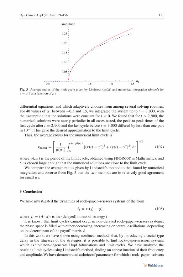
Fig. 3 Average radius of the limit cycle given by Lindstedt (solid) and numerical integration (dotted) forε = 0.1 as a function of μ1

differential equations, and which adaptively chooses from among several solving routines.For 40 values of μ1 between −0.5 and 1.5, we integrated the system up to t = 3,000, withthe assumption that the solutions were constant for t < 0. We found that for t > 2,900, thenumerical solutions were nearly periodic: in all cases tested, the peak-to-peak times of thefirst cycle after t = 2,900 and the last cycle before t = 3,000 differed by less than one partin 10−7. This gave the desired approximation to the limit cycle.

Thus, the average radius for the numerical limit cycle is

rnumer =[

1

p(μ1)

∫ t0+p(μ1)

t0

((x(t) − x∗)2 + (y(t) − y∗)2

)dt

]1/2

(107)

where p(μ1) is the period of the limit cycle, obtained using FindRoot in Mathematica, andt0 is chosen large enough that the numerical solutions are close to the limit cycle.

We compare the average radius given by Lindstedt’s method to that found by numericalintegration and observe from Fig. 3 that the two methods are in relatively good agreementfor small μ1.

3 Conclusion

We have investigated the dynamics of rock–paper–scissors systems of the form

xi = xi ( fi − φ), (108)

where fi = (A · x)i is the (delayed) fitness of strategy i .It is known that limit cycles cannot occur in non-delayed rock–paper–scissors systems;

the phase space is filled with either decreasing, increasing or neutral oscillations, dependingon the determinant of the payoff matrix A.

In this work, we have shown using nonlinear methods that, by introducing a social-typedelay in the fitnesses of the strategies, it is possible to find rock–paper-scissors systemswhich exhibit non-degenerate Hopf bifurcations and limit cycles. We have analyzed theresulting limit cycles using Lindstedt’s method, finding an approximation of their frequencyand amplitude.We have demonstrated a choice of parameters forwhich a rock–paper–scissors

152 Dyn Games Appl (2016) 6:139–156

system undergoes a supercritical Hopf bifurcation and exhibits a stable limit cycle. For thischoice of parameters, the prediction of Lindstedt’s method is found to agree with numericalintegration for T close to T0.

This generalization of the replicator model may be useful in modeling natural or socialsystems in which each player has a delayed estimate of the expected payoff of each strategy.

Appendix 1: Derivation of replicator equation

Consider an exponential model of population growth,

ξi = ξi gi (i = 1, . . . , n) (109)

where ξi is a real-valued function that approximates the population of strategy i andgi (ξ1, . . . , ξn) is the fitness of that strategy. The replicator Eq. [7] results from Eq. (109) bychanging variables from the populations ξi to the relative abundances, defined as xi ≡ ξi/pwhere p is the total population:

p(t) =∑

i

ξi (t). (110)

We see that

p =∑

i

ξi =∑

i

ξi gi (111)

= p∑

i

ξi

pgi = p

∑

i

xi gi (112)

= pφ (113)

where φ ≡ ∑i xi gi is the average fitness of the whole population.

By the product rule,

xi = ξi

p− ξi p

p2(114)

= ξi

pgi − ξi

p

p

p(115)

= xi (gi − φ) . (116)

Therefore,∑

i

xi =∑

i

xi gi − φ∑

i

xi (117)

=∑

i

xi gi −∑

j

x j g j

∑

i

xi . (118)

So, using the fact that

∑

i

xi =∑

i ξi

p= p

p≡ 1 (119)

Equation (118) reduces to the identity∑

i

xi = 0. (120)

Dyn Games Appl (2016) 6:139–156 153

The fitness of a strategy is assumed to depend only on the relative abundance of each strat-egy in the overall population, since the model only seeks to capture the effect of competitionbetween strategies, not any environmental or other factors. Therefore, we assume that gi hasthe form

gi (ξ1, . . . , ξn) = fi

(ξ1

p, . . . ,

ξn

p

)

= fi (x1, . . . , xn). (121)

Under this assumption, Eq. (116) is the replicator equation,

xi = xi ( fi − φ), (122)

where φ is now expressed entirely in terms of the xi , as

φ =∑

i

xi fi . (123)

Mathematically,φ is a coupling term that introduces dependence on the abundance and fitnessof other strategies.

Appendix 2: Coefficients generated in the RPS problem

The entries of the matrix J from Eq. (34) are

α = x∗ ((a1 − b1)(x

∗ − 1) − (a2 + b1 + b3)y∗) (124)

β = x∗ ((a1 + a3 + b2)(x

∗ − 1) + (a3 − b3)y∗) (125)

γ = y∗ ((a1 − b1)x

∗ − (a2 + b1 + b3)(y∗ − 1)

)(126)

δ = y∗ ((a1 + a3 + b2)x

∗ + (a3 − b3)(y∗ − 1)

)(127)

where x∗ and y∗ are the coordinates of the interior equilibrium point,

(x∗, y∗) =(

b3 (a3 + b2) + a1a3a1 (a2 + a3 + b1) + a2 (a3 + b2) + b3 (a3 + b1 + b2) + b1b2

,

a1 (a2 + b1) + b1b3a1 (a2 + a3 + b1) + a2 (a3 + b2) + b3 (a3 + b1 + b2) + b1b2

)

. (128)

The coefficients in Eqs. (52) and (53) are

c1 = (a1 − b1)(2x∗ − 1) − (a2 + b1 + b3)y

∗ (129)

c2 = (a1 + a3 + b2)(2x∗ − 1) + (a3 − b3)y

∗ (130)

c3 = −(a2 + b1 + b3)x∗ (131)

c4 = (a3 − b3)x∗ (132)

d1 = a1 − b1 (133)

d2 = a1 + a3 + b2 (134)

d3 = −(a2 + b1 + b3) (135)

d4 = a3 − b3 (136)

h1 = (a1 − b1)y∗ (137)

h2 = (a1 + a3 + b2)y∗ (138)

h3 = (a1 − b1)x∗ − (a2 + b1 + b3)(2y

∗ − 1) (139)

154 Dyn Games Appl (2016) 6:139–156

h4 = (a1 + a3 + b2)x∗ − (a3 − b3)(2y

∗ − 1) (140)

j1 = −(a2 + b1 + b3) (141)

j2 = a3 − b3 (142)

j3 = a1 − b1 (143)

j4 = a1 + a3 + b2. (144)

The coefficients B1, . . . , B4 in Eqs. (77) and (78) are

B1 = 1

2[s (2c4r + c2 + c3) cos(ω0T0)

− (c4(r − s)(r + s) + (c2 + c3) r + c1) sin(ω0T0)] (145)

B2 = 1

2[−s (2c4r + c2 + c3) sin(ω0T0)

− (c4(r − s)(r + s) + (c2 + c3) r + c1) cos(ω0T0)] (146)

B3 = 1

2[s (2h4r + h2 + h3) cos(ω0T0)

− (h4(r − s)(r + s) + (h2 + h3) r + h1) sin(ω0T0)] (147)

B4 = 1

2[−s (2h4r + h2 + h3) sin(ω0T0)

− (h4(r − s)(r + s) + (h2 + h3) r + h1) cos(ω0T0)] (148)

where r and s are as in Eq. (74).

Appendix 3: Removal of secular terms in Lindstedt’s method with delay

Consider a system of differential delay equations of the form

ωdu

dt= αu + βv + K1 sin t + K2 cos t (149)

ωdv

dt= γ u + δv + K3 sin t + K4 cos t. (150)

where u = u(t − ωT ) and v = v(t − ωT ), and where ω and T are such that the associatedhomogeneous problem,

ωdu

dt= αu + βv (151)

ωdv

dt= γ u + δv (152)

admits solutions of the form sin t and cos t , or equivalently ei t .Substituting u = rei t and v = sei t into Eqs. (151) and (152), we obtain the characteristic

equations

irω = e−iωT (αr + βs) (153)

isω = e−iωT (γ r + δs). (154)

Dyn Games Appl (2016) 6:139–156 155

Rearranging, these become(

αe−iωT − iω βe−iωT

γ e−iωT δe−iωT − iω

) (r

s

)

=(0

0

)

. (155)

Define

R ≡(

αe−iωT − iω βe−iωT

γ e−iωT δe−iωT − iω

)

. (156)

A non-trivial solution for r and s requires that det R = 0. Separating the real and imaginaryparts, this means that

Re(det R) = cos(2ωT )(αδ − βγ ) − ω((α + δ) sin(ωT ) + ω) = 0 (157)

Im(det R) = − cos(ωT )(sin(ωT )(2αδ − 2βγ ) + ω(α + δ)) = 0. (158)

Equation (158) tells us that

sin(ωT ) = ω(α + δ)

2(βγ − αδ). (159)

(We neglect the alternate possibility that cos(ωT ) = 0.) Then, we substitute this back intoEq. (157) to obtain

ω2 = αδ − βγ. (160)

Under the conditions (159) and (160), the solutions to Eqs. (149) and (150) will in generalhave secular terms:

u = m1 cos t + m2 sin t + n1t cos t + n2t sin t (161)

v = m3 cos t + m4 sin t + n3t cos t + n4t sin t. (162)

We wish to derive conditions on the Ki in Eqs. (149) and (150) such that the ni are all equalto 0.

We substitute the solutions (161) and (162) into Eqs. (149) and (150), and set the coeffi-cients of sin t , cos t , t sin t and t cos t separately equal to 0 in both equations.

The coefficients of sin t and cos t give us a system of linear equations on the mi and ni ,of the form

M · m + N · n = −k (163)

where m = (m1, . . . ,m4)T, n = (n1, . . . , n4)T and k = (K1, . . . , K4)

T.Similarly, the coefficients of t sin t and t cos t give us a system of linear equations on the

ni , of the form

S · n = 0. (164)

By row reducing in Mathematica, we find that both M and S have rank 2. To eliminatethe ni , we proceed as follows:

– Without loss of generality, set m3 = m4 = 0.

156 Dyn Games Appl (2016) 6:139–156

– Solve any two independent rows of Eq. (164) for n3 and n4 in terms of n1 and n2. Theresult is

n3 = n2ω cos(ωT ) − n1(α + ω sin(ωT ))

β(165)

n4 = −n1ω cos(ωT ) + n2(α + ω sin(ωT ))

β(166)

– Substitute these expressions for n3 and n4 into Eq. (163). This is now a full-rank linearsystem of equations on m1,m2, n1 and n2. Solve this system to obtain expressions form1,m2, n1 and n2 in terms of the Ki .

– Substitute the expressions for n1 and n2 from the previous step into Eqs. (165) and (166).Now we have all the ni in terms of the Ki .

– Set the ni expressions equal to 0. This gives a rank-2 system of equations on the Ki , soit is possible to solve for K3 and K4 in terms of K1 and K2. The result is

K3 = γ (K1(α + ω sin(ωT )) + K2ω cos(ωT ))

α2 + 2αω sin(ωT ) + ω2 (167)

K4 = γ (K2(α + ω sin(ωT )) − K1ω cos(ωT ))

α2 + 2αω sin(ωT ) + ω2 . (168)

Using Eqs. (159) and (160), these reduce to

K3 = K1(δ − α) − K2√−(α − δ)2 − 4βγ

2β(169)

K4 = K1√−(α − δ)2 − 4βγ + K2(δ − α)

2β. (170)

If Eqs. (169) and (170) hold, then there are solutions of Eqs. (149) and (150) with no secularterms.

References

1. Erneux T (2009) Applied differential delay equations. Springer, New York2. Guckenheimer J, Holmes P (2002) Nonlinear oscillations, dynamical systems, and bifurcations of vector

fields. Springer, New York3. Hofbauer J, SigmundK (1998) Evolutionary games and population dynamics. CambridgeUniversity Press,

Cambridge4. Miekisz J (2008) Evolutionary game theory and population dynamics. In: Multiscale Problems in the Life

Sciences. Lecture Notes in Mathematics, 1940. Springer, Berlin, pp 269–3165. Nowak M (2006) Evolutionary dynamics. Belknap Press of Harvard University Press, Cambridge6. Sigmund K (2010) Introduction to evolutionary game theory. In: K. Sigmund, (ed) Evolutionary game

dynamics, Proceedings of Symposia in Applied Mathematics, vol 69. American Mathematical Society,Providence. Paper no. 1, pp 1–26

7. Taylor P, Jonker L (1978) Evolutionarily stable strategies and game dynamics. Math Biosci 40:145–1568. Yi T, ZuwangW (1997) Effect of time delay and evolutionarily stable strategy. J Theor Biol 187(1):111–116